improving tropical forest aboveground biomass estimations
TRANSCRIPT
HAL Id: tel-02903121https://pastel.archives-ouvertes.fr/tel-02903121
Submitted on 20 Jul 2020
HAL is a multi-disciplinary open accessarchive for the deposit and dissemination of sci-entific research documents, whether they are pub-lished or not. The documents may come fromteaching and research institutions in France orabroad, or from public or private research centers.
L’archive ouverte pluridisciplinaire HAL, estdestinée au dépôt et à la diffusion de documentsscientifiques de niveau recherche, publiés ou non,émanant des établissements d’enseignement et derecherche français ou étrangers, des laboratoirespublics ou privés.
Improving tropical forest aboveground biomassestimations : insights from canopy trees structure and
spatial organizationPierre Ploton
To cite this version:Pierre Ploton. Improving tropical forest aboveground biomass estimations : insights from canopytrees structure and spatial organization. Biodiversity and Ecology. AgroParisTech; Technische Uni-versität (Dresde, Allemagne). Institut für Kartographie, 2017. English. �NNT : 2017AGPT0005�.�tel-02903121�
AgroParisTech - IRD Unité Mixte de Recherche AMAP
TA A-51 / PS1 Bd de la Lironde, 34398 Montpellier cedex 5, FRANCE
N°: 2017AGPT0005
présentée et soutenue publiquement par
Pierre PLOTON
le 27 Mars 2017
Improving tropical forest aboveground biomass estimations:
insights from canopy trees structure and spatial organization
Doctorat AgroParisTech
T H È S E
pour obtenir le grade de docteur délivré par
L’Institut des Sciences et Industries du Vivant et de l’Environnement
(AgroParisTech)
Spécialité : Ecologie et Biodiversité
Directeur de thèse : Dr. Raphaël PELISSIER Co-encadrement de la thèse : Prof. Dr. Uta BERGER
Jury M. Lilian BLANC, Chercheur (HDR), CIRAD Rapporteur
M. Laurent SAINT-ANDRE, Directeur de Recherche, INRA Rapporteur
M. Hans-Gerd MAAS, Professeur, Technische Universität Dresden Rapporteur
M. Pierre COUTERON, Directeur de Recherche, IRD Président
Mme Uta BERGER, Professeur, Technische Universität Dresden Co-directeur de thèse
M. Raphaël PELISSIER, Directeur de Recherche, IRD Directeur de thèse


ACKNOWLEDGEMENTS
This doctoral thesis was realized thanks to the support of the 2013-2016 Forest, Nature and Society
(FONASO) grant, funded by the European Commission’s Erasmus Mundus Joint Doctorate
programme (EMJD). Part of the thesis was funded by the CoForTips project as part of the ERA-Net
BiodivERsA 2011-2012 European joint call (ANR-12-EBID-0002). I am also grateful for the multiple
travelling funds I received from the UMR AMAP of the French Institut de Recherche pour le
Développement (IRD).
I have benefited from the support, advices and help of numerous people during the 3 (and a half…)
years of this PhD project. First and foremost, I would like to thank Dr. Raphaël Pélissier, who’s been
supervising my work since my first steps in the world of forest research, about 7 years ago at the
French Institute of Pondicherry. I’m deeply indebted to you for the opportunity you gave me to work
on such fascinating subjects during the past years. For your incredible patience while reading long
and sometimes crazy “results syntheses” I’ve been sending you, for helping me to see broader
implications rather than details in my analyses, for your positive attitude toward our findings, thank
you. I am also very grateful to Prof. Uta Berger, who kindly provided support and guidance during this
project, and made this Joint Doctoral Programme a very positive experience for me.
I must also warmly thank Dr. Nicolas Barbier for the considerable amount of time we spent, at the
office or in the field, brainstorming about our common research interests. Beyond invaluable
scientific guidance, total availability for my questions and concerns, deep involvement in the
different projects we undertook, you’ve simply been of great company, and I’m thankful for the tons
of fun we had in the field.
This list is far from being exhaustive, but I should also mention my deep gratitude to Dr. Pierre
Couteron, Dr. Christophe Proisy and Dr. Maxime Réjou-Méchain for the fruitful discussions we had,
notably on FOTO texture and biomass allometric models. I am also very grateful to Dr. Gilles Le
Moguedec for his availability and good will to help me resolve statistical issues I’ve been having
throughout this project.
Last but not least, this PhD project largely beneficiated from the field work several colleagues and I
carried out in Cameroon. I owe a great deal of thanks to Prof. Bonaventure Sonké, who warmly
welcomed me in his research team and created a pleasant and efficient working environment. I’d
also like to thank Dr. Vincent Droissart with whom, just like with Nicolas, I spent a formidable time in
the field. My thoughts also go to the Cameroonian students and friends I’ve been collecting field data
with, notably S.T. Momo, M. Libalah, N.G. Kamdem, H. Taedoumg, G. Kamdem Meikeu and D.
Zebaze.

TABLE OF CONTENTS
1 GENERAL INTRODUCTION..................................................................................................................1
1.1 Context and challenges .................................................................................................................1
1.1.1 Tropical forests and climate change ....................................................................................1
1.1.2 REDD monitoring frame of tropical forest biomass: basics and challenges ..........................2
1.1.3 Remote sensing-based modelling of tropical forest biomass ...............................................4
1.2 Research objectives.......................................................................................................................8
1.3 A pantropical approach .................................................................................................................9
1.3.1 Study areas and datasets ....................................................................................................9
1.3.2 Sampling strategy and data description ............................................................................ 11
1.4 Thesis outline .............................................................................................................................. 12
1.5 List of (co-)publications ............................................................................................................... 13
1.6 References .................................................................................................................................. 14
2 CLOSING A GAP IN TROPICAL FOREST BIOMASS ESTIMATION: ACCOUNTING FOR CROWN MASS VARIATION IN
PANTROPICAL ALLOMETRIES .................................................................................................................... 19
2.1 Introduction .......................................................................................................................... 20
2.2 Materials and Methods ......................................................................................................... 22
2.2.1 Biomass data ............................................................................................................. 22
2.2.2 Forest inventory data ................................................................................................. 22
2.2.3 Allometric model fitting ............................................................................................. 22
2.2.4 Development of crown mass proxies.......................................................................... 23
2.2.5 Model error evaluation .............................................................................................. 24
2.3 Results .................................................................................................................................. 25
2.3.1 Contribution of crown to tree mass............................................................................ 25
2.3.2 Crown mass sub-models ............................................................................................ 25
2.3.3 Accounting for crown mass in biomass allometric models .......................................... 28
2.4 Discussion ............................................................................................................................. 32
2.4.1 Crown mass ratio and the reference biomass model error ......................................... 32
2.4.2 Model error propagation depends on targeted plot structure .................................... 33
2.4.3 Accounting for crown mass variation in allometric models ......................................... 33
2.5 Appendix A: Crown mass sub-models .................................................................................... 34
2.5.1 Method...................................................................................................................... 34
2.5.2 Results & Discussion .................................................................................................. 34
2.6 Appendix B: Plot-level error propagation ............................................................................... 38
2.7 References ............................................................................................................................ 41
2.8 Supplement: Field data protocols .......................................................................................... 46
2.8.1 Unpublished dataset: site characteristics ................................................................... 46
2.8.2 Biomass data ............................................................................................................. 46
2.8.3 Inventory data ........................................................................................................... 48
3 ASSESSING DA VINCI’S RULE ON LARGE TROPICAL TREE CROWNS OF CONTRASTED ARCHITECTURES: EVIDENCE FOR
AREA-INCREASING BRANCHING ................................................................................................................ 49
3.1 Introduction .......................................................................................................................... 49
3.2 Methods ............................................................................................................................... 51
3.2.1 Sampled trees and field protocol ............................................................................... 51
3.2.2 MTE model assumptions and predictions of branch scaling exponents ....................... 53
3.2.3 Assessing the effect of asymmetry and node morphology on species area ratio ......... 54
3.3 Results .................................................................................................................................. 55
3.3.1 Does the average tree conform to branch scaling exponents and area ratio predictions?
.................................................................................................................................. 55
3.3.2 Is the average tree self-similar?.................................................................................. 55
3.3.3 What is the effect of species asymmetry on branch scaling exponents and area ratio? .
.................................................................................................................................. 56
3.3.4 Does node morphology induce systematic differences of area ratio at the species level?
.................................................................................................................................. 58
3.4 Discussion ............................................................................................................................. 59
3.4.1 Evidence of area increasing branching (R > 1) ............................................................. 59
3.4.2 Sources of variation of the node area ratio ................................................................ 60
3.4.3 Optimal tree of the MTE model vs average real trees ................................................. 62
3.4.4 Implications of the results .......................................................................................... 64
3.5. Reference................................................................................................................................... 65
3.6. Supplementary figure ................................................................................................................. 68
4 CANOPY TEXTURE ANALYSIS FOR LARGE-SCALE ASSESSMENTS OF TROPICAL FOREST STAND STRUCTURE AND
BIOMASS ............................................................................................................................................. 69
4.1 Introduction .......................................................................................................................... 70
4.2 Methodological background and rationale ............................................................................ 70
4.3 Results from some case studies ............................................................................................. 72
4.4 Limits and perspectives ......................................................................................................... 75
4.5 Reference .............................................................................................................................. 76
5 TOWARD A GENERAL TROPICAL FOREST BIOMASS PREDICTION MODEL FROM VERY HIGH RESOLUTION OPTICAL
SATELLITE IMAGES ................................................................................................................................. 77
Abstract ............................................................................................................................................ 77
5.1 Introduction .......................................................................................................................... 78
5.2 Material and Methods ........................................................................................................... 80
5.2.1 Forest inventory data ................................................................................................. 80
5.2.2 Generation of 3D forest mockups .............................................................................. 81
5.2.3 Simulation of canopy images...................................................................................... 82
5.2.4 Real satellite images .................................................................................................. 82
5.2.5 Canopy texture analysis ............................................................................................. 83
5.2.6 Statistical analyses ..................................................................................................... 84
5.3 Results .................................................................................................................................. 85
5.3.1 Texture analysis of virtual canopy images .................................................................. 85
5.3.2 Canopy texture - AGB models .................................................................................... 89
5.3.3 Application to real satellite images............................................................................. 91
5.4 Discussion ............................................................................................................................. 91
5.4.1 Contrasted canopy texture - stand AGB relationships among sites ............................. 92
5.4.2 On 3D stand mockups and virtual canopy images for model calibration ..................... 93
5.5 Reference .............................................................................................................................. 95
5.6 Appendix ............................................................................................................................. 100
6 GENERAL DISCUSSION .................................................................................................................. 102
6.1 Estimation of forest AGB from field data ............................................................................. 102
6.1.1 Driver(s) of pantropical model bias on large trees .................................................... 102
6.1.2 The influence of forest structure on plot-level AGB modelling error ......................... 105
6.2 The influence of forest structure on the canopy texture – AGB relationship ........................ 106
6.3 Key thesis findings ............................................................................................................... 110
6.4 Reference ............................................................................................................................ 111
LIST OF FIGURES
Figure 1-1. General workflow of remote sensing-based AGB mapping methods. Regardless of the remote
sensing data type, remote sensing indice(s) are extracted over forest sample plots (A) and used a
predictor(s) of in situ AGB estimations (B). Once calibrated, the model can be used to predict forest
AGB over the entire study area (C). .....................................................................................................4
Figure 1-2. Schematic illustration of virtual canopy scenes simulation procedure. Field inventory data are
used in a forest model to generate 3D mockups of the sample plots. A radiative transfer model
simulates a satellite view of the mockups, for instance a VHSR 1-m IKONOS panchromatic channel. ...6
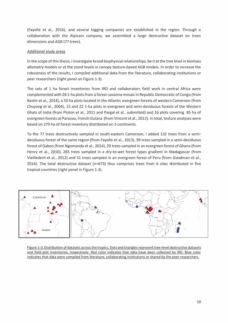
Figure 1-3. Distribution of datasets across the tropics. Dots and triangles represent tree-level destructive
datasets and field plot inventories, respectively. Red color indicates that data have been collected by
IRD. Blue color indicates that data were compiled from literature, collaborating institutions or shared
by the peer researchers. ................................................................................................................... 10
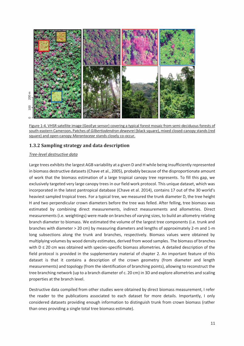
Figure 1-4. VHSR satellite image (GeoEye sensor) covering a typical forest mosaic from semi-deciduous
forests of south-eastern Cameroon. Patches of Gilbertiodendron dewevrei (black square), mixed
closed-canopy stands (red square) and open-canopy Marantaceae stands closely co-occur. ............. 11
Figure 2-1. (A) Distribution of crown mass ratio (in %) along the range of tree mass (TAGBobs, in Mg) for
673 trees. Dashed lines represent the fit of robust regressions (model II linear regression fitted using
ordinary least square) performed on the full crown mass dataset (thick line; one-tailed permutation
test on slope: p-value < 0.001) and on each separate source (thin lines), with symbols indicating the
source: empty circles from Vieilledent et.al. (2011; regression line not represented since the largest
tree is 3.7 Mg only); solid circles from Fayolle et.al. (2013); squares from Goodman et al. (2013, 2014);
diamonds from Henry et.al. (2010); head-up triangles from Ngomanda et.al. (2014); and head-down
triangles from the un-published data set from Cameroon. (B) Boxplot representing the variation in
crown mass ratio (in %) across tree mass bins of equal width (2.5 Mg). The last bin contains all trees ≥
20 Mg. The number of individuals per bin and the results of non-parametric pairwise comparisons are
represented below and above the median lines, respectively. .......................................................... 26
Figure 2-2. (A) Observed crown mass versus the compound variable D²Hcρ (in log scale), displaying a
slightly concave relationship. The crown mass sub-model 1 does not capture this effect (model fit
represented with a full line in caption A), resulting in biased model predictions (caption B), whereas
sub-model 3 does not present this error pattern (model fit represented as a dashed line in caption A,
observed crown mass against model predictions in caption C). Models were fitted on DataCM2. ........ 28
Figure 2-3. (A) Relative individual residuals (si in %) of the reference pantropical model of Chave et.al.
(2014) against the tree AGB gradient. The thick dashed line represents the fit of a local regression (loess
function, span = 0.5) bounded by standard errors. (B) Observed tree AGB (TAGBobs) versus the
compound variable !2 " # " $ with D and H being the tree stem diameter and height, respectively,
and ρ the wood density. A segmented regression revealed a significant break point (thin vertical
dashed line) at approximately 10 Mg of TAGBobs (Davies test p-value < 2.2e-16). .............................. 29
Figure 2-4. (A) Relative residuals (si, in %) of the reference pantropical model m0 (grey background) and
our model m1 including crown mass (white background). Thick dashed lines represent fits of local
regressions (loess function, span = 1) bounded by standard errors. (B) Propagation of individual
estimation errors of m0 (solid grey circles) and m1 (empty circles) to the plot level. .......................... 29
Figure 2-5. (A) Relative individual residuals (si, in %) obtained with the reference pantropical model m0
(grey background) and with our model including a crown mass proxy, m2 (white background). Thick
dashed lines represent fits of local regressions (loess function, span = 1) bounded by standard errors.
(B) Propagation of individual residual errors of m0 (solid grey circles) and m2 (empty circles) to the plot
level. ................................................................................................................................................. 30
Figure 2-6. Observed against estimated crown mass (in Mg) for models 1-D (caption A), 1-Hc (caption B),
2-D (caption C), 3 (caption D). Models were calibrated on DataCM2. Tree wood density was standardized
to range between 0 and 1 and represented as a grayscale (with black the lowest values and white the
highest values). ................................................................................................................................. 35
Figure 2-7. Observed versus estimated crown mass (in Mg) for models 1-D (caption A), 1-Cd (caption B),
2-D (caption C), 2-Cd (caption D). Models were calibrated on DataCD. Tree wood density was
standardized to range between 0 and 1 and is represented as a grayscale (with black the lowest values
and white the highest values). .......................................................................................................... 37
Figure 2-8. Plot-level propagation of individual-level model error. (A) Mean relative error (Splot, in %) and
standard deviation of 1000 random error sampling against simulated plot AGB and (B) against the
fraction (%) of simulated plot AGB accounted for by trees > 20 Mg. Plots from Korup permanent plot
are represented by triangles. ............................................................................................................ 39
Figure 2-9. Plot-level relative error (Splot, in %) as a function of plot size (in ha) in Korup permanent plot.
Individual plot values are represented by grey dots. ......................................................................... 39
Figure 3-1. Schematic representation of different levels of asymmetry in species’ architecture, from the
optimal MTE tree (A) to moderately (B) and highly (C) dominant apex. O1 to O4 represent the labeling
scheme of the MTE. In panel C, Om1 to Om2 illustrate a modified labeling scheme accounting for the
presence of a principal axis in tree crown structure (see text). The right column gives illustrations of
the three types of architectures based on large canopy tree species from central Africa, from top to
bottom: Okan, Ayous and Ilomba (see Table 3-1 for more information on these species). ................. 52
Figure 3-2. Distribution of sampled nodes along node parent diameters (in cm) in each of the 9 sampled
species. ............................................................................................................................................. 52
Figure 3-3. Frequency of PA internodes per species. Ilomba (35.7% : highly asymmetric), Ayous (9.4% :
moderately asymmetric) and Okan (1.3%: symmetric) were selected as illustrative species in results
sections 3.3 and 3.4. ......................................................................................................................... 54
Figure 3-4. Density distributions (standardized to 1) of internodes length scaling exponents (A), radii
scaling exponents (B) and nodes area ratios (C) at the inter-specific level. Dash lines represent the
expected values under the Metabolic Theory of Ecology, while grey bars represent the 95% confidence
interval of resampled medians (A, B) and mean (C). .......................................................................... 55
Figure 3-5. Density distributions (standardized to 1) of internodes length scaling exponents (A), radii
scaling exponents (B) and nodes area ratios (C) across the first orders (i.e. 2, 3, ≥ 4) of the centrifugal
labeling scheme. We excluded internodes of parent order 1 (i.e., the trunk) from analysis of length
scaling exponents (in panel A). Dash black lines represent the expected values for hierarchical,
symmetric, self-similar trees. Color bars represent the 2.5-97.5% interval of resampled medians per
group. Branch scaling exponents and area ratios are also represented against parent diameter (D, E,
F). ..................................................................................................................................................... 56
Figure 3-6. Density distributions (standardized to 1) of internode length scaling exponents (A, B),
internodes radii scaling exponents (C, D) and node area ratios (E,F). In plots A, C and E, parameters are
given for 3 illustrative species (i.e., Ayous, Ilomba and Okan) with contrasted frequency of PA
internodes (cf. fig 3). Distributions are based on all internodes and nodes from those species,
regardless of node morphology. In plots B, D and F, distributions are based on all data (inter-specific)
split by node morphology i.e., internodes and nodes were grouped according to the presence of a PA,
thus differentiating PA branches, their sibling(s) and branches from nodes w/o PA branch (noted
“Other”). Dash black lines represent the expected values for hierarchical, symmetric, self-similar trees.
Color bars represent the 2.5-97.5% interval of resampled medians per group. .................................. 57
Figure 3-7. (A) Density distribution of nodes area ratio for nodes with 2 (light grey) and >2 daughters (dark
grey). (B) Nodes area ratio against daughters asymmetry (‘q’). Thick and thin dashed lines represent
fits of linear models on nodes bearing (dark grey) or not bearing (light grey) PA branches, respectively.
(C, D) Daughters cumulated area against parent area (in true unit). The upper limits of plots axes was
set to 1.5 m² to ease species comparison, as branch cross-sectional areas for the Ayous species extend
above c. 2.5 m². Dashed lines represent the fits of linear models on both Ayous and Ilomba (black line)
and Okan (grey line). Linear models were adjusted on log-transformed data. ................................... 59
Figure 3-8. Histograms of log-transformed abundance against log-transform branch diameter (panel A)
and branch length (panel B) for all nine species. Daughters dimensions (diameter, length) against
parents dimensions (diameter length) are represented in panel C and D, with a color code
differentiating PA daughters (solid black circles) from other daughters (solid grey circles). In panel E
and F, the number of daughters (nD) is represented against parent order and per illustrative species,
respectively. In panel E, the labelling scheme used to defined parent order is either the centrifugal
scheme of the MTE (solid black circles) or the modified labelling scheme distinguishing PA daughters
(order 1), their siblings (order 2) and other daughters (order ≥ 3) (empty circles). In panel F, a distinction
is made between nodes bearing PA daughters (solid black circles) and others nodes (empty circles).
Letters represent the result of Dunn pairwise multiple comparisons tests......................................... 68
Figure 4-1. Flow of operations of the FOurier Textural Ordination (FOTO) method. ................................ 72
Figure 5-1. Canopy texture ordinations based on (A) the FOTO method and (B) the lacunarity analysis. In
both cases, scatter plots of PCA scores along the first two principal axes are shown, with 3 example
sites highlighted with particular symbols (Paracou, Uppangala and Yellapur). Correlation circles are
given with wavelength, λ (A) or box size, s (B) in meter. Histograms of eigenvalues in % of total variance.
......................................................................................................................................................... 86
Figure 5-2. Co-inertia analysis. Position on the first co-inertia plane of the FOTO r-spectra wavelengths, λ
(A) and the lacunarity box size, s (D). Components of the F-PCA (B) and the L-PCA (E) projected onto
the co-inertia axes. Ordination of windows from the 3 example sites (Paracou, Uppangala and Yellapur)
on COIA-1 (C) with large empty and full circles representing the average site-level score for FOTO and
Lacunarity features, respectively. Normed scores of 10 randomly sampled canopy windows from the 3
example sites on the first co-inertia plane (F), with each arrow linking a canopy window position for
FOTO and Lacunarity characteristics, respectively. ............................................................................ 89
Figure 5-3. Multi-site AGB prediction models based on FOTO texture (F-model), Lacunarity texture (L-
model), the two sources of texture information (FL-model) to which we also added a forest canopy
height proxy E (FLE-model). Texture features were extracted from virtual canopy scenes. Goodness of
fit statistics are defined in Methods section. ..................................................................................... 90

Figure 5-4. Multi-site AGB prediction model over 49 1-ha plots in central Africa, based on both FOTO-
texture and Lacunarity-texture indices to which we added the bioclimatic stress variable E as a proxy
of potential canopy height (FLE-model). ............................................................................................ 91
Figure 6-1. Field-derived AGB vs AGB predicted from the pantropical model of Chave et. al (2014). Circles
represent the trees of Chave et al. (2014) destructive database, with the red color highlighting the
trees sampled in the frame of this thesis. Stars represent Entandrophragma excelsum individuals
sampled by Hemp et al. (2016)........................................................................................................ 105
Figure 6-2. Tree density (N) against quadratic mean diameter (Dg) at two sites (black: Paracou, blue: Deng-
Deng). Grey dot lines represent basal area (G) isolines. ................................................................... 108
LIST OF TABLES
Table 2-1. Crown mas sub-models. Model variables are Cm (crown mass, Mg), D (diameter at breast
height, cm), Hc (crown depth, m), Cs (average of Hc and crown diameter, m) and ρ (wood density,
g.cm-3). The general form of the models is ln(Y) ~a+ b* ln(X) + c*ln(X)². Model coefficient estimates
are provided along with the associated standard error denoted SEi, with i as the coefficient.
Coefficients’ probability value (pv) is not reported when pv ≤ 10-4 and otherwise coded as follows:
pv ≤ 10-3 : '**', pv ≤ 10-2 : '*', pv ≤ 0.05 : '.' and pv ≥ 0.05 : 'ns'. Models’ performance parameters
are R² (adjusted R square), RSE (residual standard error), S (median of unsigned relative individual
errors, in %), AIC (Akaike Information Criterion), dF (degree of freedom). .................................... 27
Table 2-2. Models used to estimate tree AGB. Model parameters are D (diameter at breast height, cm),
H (total height, m), Ht (trunk height, m), Hc (crown depth, m), Cm (crown mass, Mg), Cs (average of
Hc and crown diameter, m) and ρ (wood density, g.cm-3). The general form of the models is ln(Y)
~a+ b* ln(X1) + c*ln(X2). Model coefficient estimates are provided along with the associated
standard error denoted SEi, with i as the coefficient. Coefficients’ probability value (pv) is not
reported when pv ≤ 10-4 and otherwise coded as follows: pv ≤ 10-3 : '**', pv ≤ 10-2 : '*', pv ≤ 0.05 : '.'
and pv ≥ 0.05 : 'ns'. Models’ performance parameters are R² (adjusted R square), RSE (residual
standard error), S (median of unsigned relative individual errors, in %), AIC (Akaike Information
Criterion), dF (degree of freedom). .............................................................................................. 31
Table 2-3. Sub-models used to estimate crown AGB. Model parameters are D (diameter at breast
height, cm), Hc (crown depth, m), Cm (crown mass, Mg), Cd (crown diameter, in m), Cs (average of
Hc and Cd, m) and ρ (wood density, g.cm-3). The general form of the models is ln(Y) ~ a + b*ln(X) +
c*ln(Y). Model coefficients’ estimates are provided along with the associated standard error
denoted SEi, with i as the coefficient. Coefficients’ probability value (pv) is not reported when pv ≤
10-4 and otherwise coded as follows: pv ≤ 10-3 : '**', pv ≤ 10-2 : '*', pv ≤ 0.05 : '.' and pv ≥ 0.05 : 'ns'.
Models’ performance parameters are R² (adjusted R square), RSE (residual standard error), S
(median of unsigned relative individual errors, in %), AIC (Akaike Information Criterion), dF (degree
of freedom).................................................................................................................................. 36
Table 2-4. Six destructive datasets providing information on tree crown were combined into three
working datasets with increasing level of information. DataCM1 possess information on crown mass.
DataCM2 add information on trunk height. DataCD add information on crown diameter. ................ 47
Table 3-1. Number of trees sampled (ntree) among species, ranges of diameter at breast height (DBH,
in cm) and apical dominance (from A low dominance to C highly dominant; see Figure 3-1 for
illustration). ................................................................................................................................. 51
Table 4-1. FOTO explanatory power on several common forest stand attributes over a variety of
tropical forest types. Quality of the relationships is characterized by the coefficient of
determination (R²), the associated P-value (ns: > 0.05) and the relative root mean square error
Rrmse (in %). Forest attributes: N = density of trees more than 10 cm dbh (trees.ha-1), N30 = density
of trees more than 30 cm dbh (trees.ha-1), N100 = density of trees more than 100 cm dbh (trees.ha-
1), Dmax = maximum tree dbh (cm), Dg = quadratic mean dbh (cm), G = basal area (m².ha-1),
AGB = aboveground biomass (Mg.ha-1 dry matter), Cd = mean crown diameter (m), H = dominant
tree height (m). ............................................................................................................................ 74
Table 5-1. Date and acquisition parameters of Pleiades panchromatic satellite images over Eastern
Cameroun, central Africa ............................................................................................................. 83
Table 5-2. Correlation between stand structure parameters extracted from three-dimensional
mockups and canopy window scores on the texture ordination axes based on the FOTO method (F-
PCA1 and F-PCA2) and the lacunarity analysis (L-PCA1 and L-PCA2). Probability value of Pearson
correlation test are provided between brackets and coded following standard notation (*** P ≤
0.01, ** P ≤ 0.01, * P ≤ 0.05, ns = non-significant). ....................................................................... 88
Table 5-3. Distribution of forest inventory data among sampling sites. Tree dimensions collected in
field plots include the diameter at breast height (D), tree height (H), trunk height (Ht) and crown
diameter (Cd). ............................................................................................................................ 100
Table 5-4. Importance of predictors (ie. IncMSE, in %) in RF regression models calibrated on simulated
canopy scenes. Model m1 is based on FOTO-texture, m2 on Lacunarity-texture, m3 on FOTO- and
Lacunarity-texture, m4 all textural indices and the bioclimatic variable E. F-PCA1 and F-PCA2
represent the 2 FOTO-texture indices. L-PCA1 and L-PCA2 represent the 2 Lacunarity-texture
indices. ...................................................................................................................................... 101
Table 5-5. Importance of predictors (ie. IncMSE, in %) in RF regression models calibrated on real
satellite images. Model m1 is based on FOTO-texture, m2 on Lacunarity-texture, m3 on FOTO- and
Lacunarity-texture, m4 all textural indices and the bioclimatic variable E. F-PCA1 and F-PCA2
represent the 2 FOTO-texture indices. L-PCA1 and L-PCA2 represent the 2 Lacunarity-texture
indices. ...................................................................................................................................... 101
1
1 GENERAL INTRODUCTION
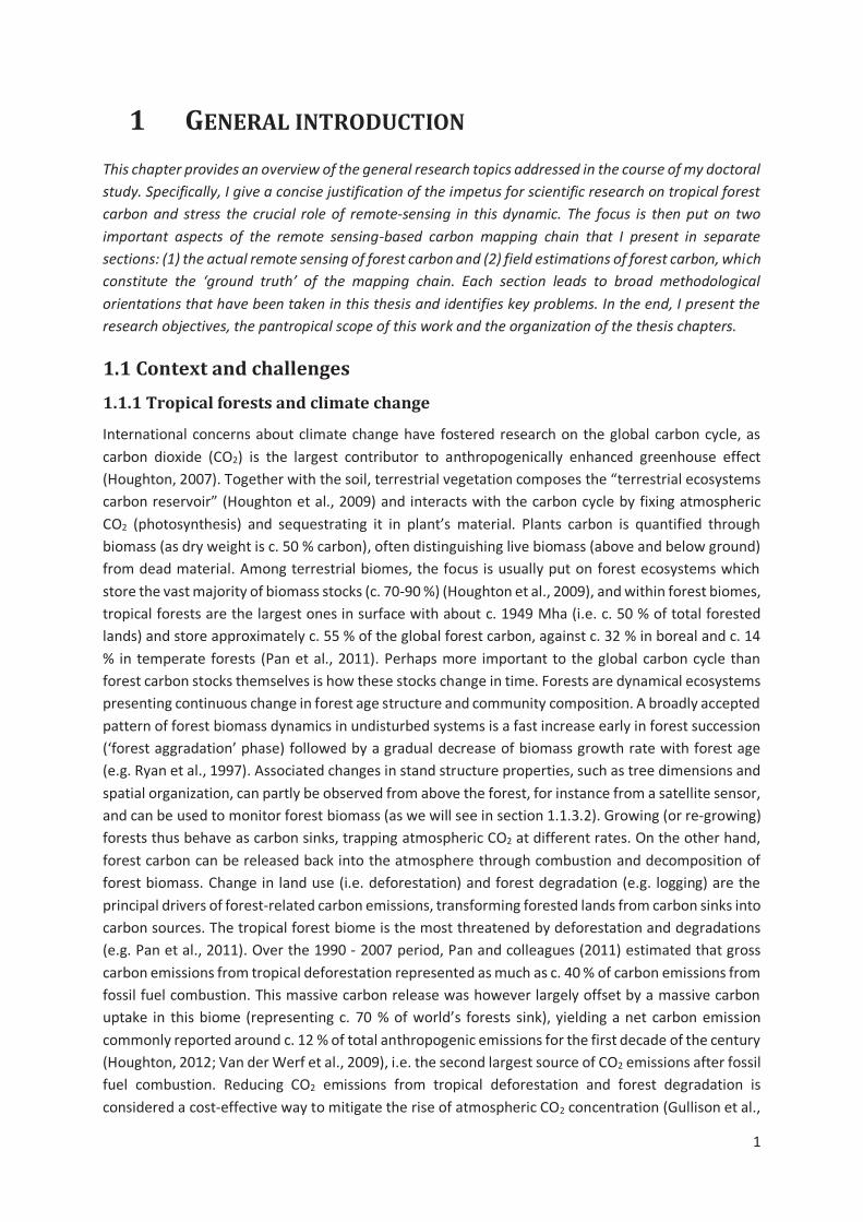
This chapter provides an overview of the general research topics addressed in the course of my doctoral
study. Specifically, I give a concise justification of the impetus for scientific research on tropical forest
carbon and stress the crucial role of remote-sensing in this dynamic. The focus is then put on two
important aspects of the remote sensing-based carbon mapping chain that I present in separate
sections: (1) the actual remote sensing of forest carbon and (2) field estimations of forest carbon, which
constitute the ‘ground truth’ of the mapping chain. Each section leads to broad methodological
orientations that have been taken in this thesis and identifies key problems. In the end, I present the
research objectives, the pantropical scope of this work and the organization of the thesis chapters.
1.1 Context and challenges
1.1.1 Tropical forests and climate change
International concerns about climate change have fostered research on the global carbon cycle, as
carbon dioxide (CO2) is the largest contributor to anthropogenically enhanced greenhouse effect
(Houghton, 2007). Together with the soil, terrestrial vegetation composes the “terrestrial ecosystems
carbon reservoir” (Houghton et al., 2009) and interacts with the carbon cycle by fixing atmospheric
CO2 (photosynthesis) and sequestrating it in plant’s material. Plants carbon is quantified through
biomass (as dry weight is c. 50 % carbon), often distinguishing live biomass (above and below ground)
from dead material. Among terrestrial biomes, the focus is usually put on forest ecosystems which
store the vast majority of biomass stocks (c. 70-90 %) (Houghton et al., 2009), and within forest biomes,
tropical forests are the largest ones in surface with about c. 1949 Mha (i.e. c. 50 % of total forested
lands) and store approximately c. 55 % of the global forest carbon, against c. 32 % in boreal and c. 14
% in temperate forests (Pan et al., 2011). Perhaps more important to the global carbon cycle than
forest carbon stocks themselves is how these stocks change in time. Forests are dynamical ecosystems
presenting continuous change in forest age structure and community composition. A broadly accepted
pattern of forest biomass dynamics in undisturbed systems is a fast increase early in forest succession
(‘forest aggradation’ phase) followed by a gradual decrease of biomass growth rate with forest age
(e.g. Ryan et al., 1997). Associated changes in stand structure properties, such as tree dimensions and
spatial organization, can partly be observed from above the forest, for instance from a satellite sensor,
and can be used to monitor forest biomass (as we will see in section 1.1.3.2). Growing (or re-growing)
forests thus behave as carbon sinks, trapping atmospheric CO2 at different rates. On the other hand,
forest carbon can be released back into the atmosphere through combustion and decomposition of
forest biomass. Change in land use (i.e. deforestation) and forest degradation (e.g. logging) are the
principal drivers of forest-related carbon emissions, transforming forested lands from carbon sinks into
carbon sources. The tropical forest biome is the most threatened by deforestation and degradations
(e.g. Pan et al., 2011). Over the 1990 - 2007 period, Pan and colleagues (2011) estimated that gross
carbon emissions from tropical deforestation represented as much as c. 40 % of carbon emissions from
fossil fuel combustion. This massive carbon release was however largely offset by a massive carbon
uptake in this biome (representing c. 70 % of world’s forests sink), yielding a net carbon emission
commonly reported around c. 12 % of total anthropogenic emissions for the first decade of the century
(Houghton, 2012; Van der Werf et al., 2009), i.e. the second largest source of CO2 emissions after fossil
fuel combustion. Reducing CO2 emissions from tropical deforestation and forest degradation is
considered a cost-effective way to mitigate the rise of atmospheric CO2 concentration (Gullison et al.,
2
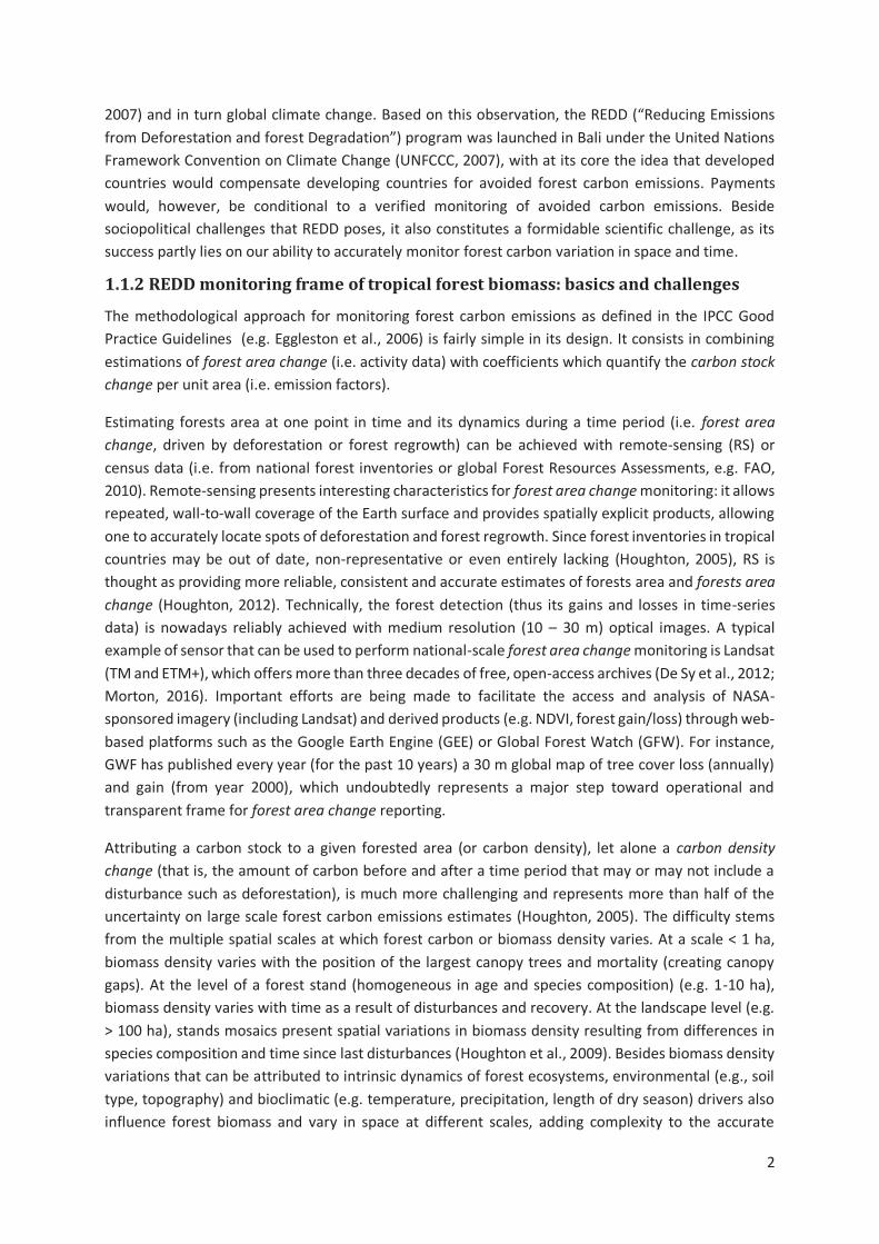
2007) and in turn global climate change. Based on this observation, the REDD (“Reducing Emissions
from Deforestation and forest Degradation”) program was launched in Bali under the United Nations
Framework Convention on Climate Change (UNFCCC, 2007), with at its core the idea that developed
countries would compensate developing countries for avoided forest carbon emissions. Payments
would, however, be conditional to a verified monitoring of avoided carbon emissions. Beside
sociopolitical challenges that REDD poses, it also constitutes a formidable scientific challenge, as its
success partly lies on our ability to accurately monitor forest carbon variation in space and time.
1.1.2 REDD monitoring frame of tropical forest biomass: basics and challenges
The methodological approach for monitoring forest carbon emissions as defined in the IPCC Good
Practice Guidelines (e.g. Eggleston et al., 2006) is fairly simple in its design. It consists in combining
estimations of forest area change (i.e. activity data) with coefficients which quantify the carbon stock
change per unit area (i.e. emission factors).
Estimating forests area at one point in time and its dynamics during a time period (i.e. forest area
change, driven by deforestation or forest regrowth) can be achieved with remote-sensing (RS) or
census data (i.e. from national forest inventories or global Forest Resources Assessments, e.g. FAO,
2010). Remote-sensing presents interesting characteristics for forest area change monitoring: it allows
repeated, wall-to-wall coverage of the Earth surface and provides spatially explicit products, allowing
one to accurately locate spots of deforestation and forest regrowth. Since forest inventories in tropical
countries may be out of date, non-representative or even entirely lacking (Houghton, 2005), RS is
thought as providing more reliable, consistent and accurate estimates of forests area and forests area
change (Houghton, 2012). Technically, the forest detection (thus its gains and losses in time-series
data) is nowadays reliably achieved with medium resolution (10 – 30 m) optical images. A typical
example of sensor that can be used to perform national-scale forest area change monitoring is Landsat
(TM and ETM+), which offers more than three decades of free, open-access archives (De Sy et al., 2012;
Morton, 2016). Important efforts are being made to facilitate the access and analysis of NASA-
sponsored imagery (including Landsat) and derived products (e.g. NDVI, forest gain/loss) through web-
based platforms such as the Google Earth Engine (GEE) or Global Forest Watch (GFW). For instance,
GWF has published every year (for the past 10 years) a 30 m global map of tree cover loss (annually)
and gain (from year 2000), which undoubtedly represents a major step toward operational and
transparent frame for forest area change reporting.
Attributing a carbon stock to a given forested area (or carbon density), let alone a carbon density
change (that is, the amount of carbon before and after a time period that may or may not include a
disturbance such as deforestation), is much more challenging and represents more than half of the
uncertainty on large scale forest carbon emissions estimates (Houghton, 2005). The difficulty stems
from the multiple spatial scales at which forest carbon or biomass density varies. At a scale < 1 ha,
biomass density varies with the position of the largest canopy trees and mortality (creating canopy
gaps). At the level of a forest stand (homogeneous in age and species composition) (e.g. 1-10 ha),
biomass density varies with time as a result of disturbances and recovery. At the landscape level (e.g.
> 100 ha), stands mosaics present spatial variations in biomass density resulting from differences in
species composition and time since last disturbances (Houghton et al., 2009). Besides biomass density
variations that can be attributed to intrinsic dynamics of forest ecosystems, environmental (e.g., soil
type, topography) and bioclimatic (e.g. temperature, precipitation, length of dry season) drivers also
influence forest biomass and vary in space at different scales, adding complexity to the accurate
3
estimation of biomass density for a given area. From a practical point of view, methods used to
estimate biomass density can broadly be categorized into non-spatial and spatial methods. Non-spatial
methods are based on a predefined classification of forest types (“land cover map”) and consist in
attributing to each type an average biomass density derived from forest inventory data or from the
literature. This is the simplest approach that the IPCC declined in its guidelines in two different tiers of
quality: Tier 1 when broad continental forest types are used (i.e. default forest strata and associated
biomass densities) and Tier 2 when country-specific data are used (i.e. refined forest strata and
biomass densities derived from national forest inventories). With such methods, the question of
representativity of average biomass density estimates is indeed central and constitutes an obvious
source of error in carbon stock and carbon stock change estimations, especially in the tropics given the
paucity of forest inventories (e.g. Mattsson et al., 2016). Spatial methods produce biomass density
maps based on a relationship between in situ biomass estimations and bioclimatic and environmental
data, RS data, or both. When spatially explicit models are sufficiently accurate and precise (which is
commonly interpreted as “when estimation uncertainty is no more than 20 % of the mean”, Zolkos et
al., 2013), this approach would correspond to the highest quality tier of the IPCC (Tier 3). Biomass
density maps can be used to improve the representativity of average biomass density estimates used
in non-spatial methods (e.g. Langner et al., 2014) or replace them altogether. Indeed, using biomass
densities that are co-located with areas undergoing changes (e.g. deforestation) should yield more
accurate estimates of emissions (Houghton, 2012).
The REDD methodological framework requires monitoring forest carbon stock changes at large spatial
scale (regional, national) to limit the so-called leakage phenomenon, whereby deforestation and
degradations would simply be displaced from a protected area to elsewhere. At such a large scale, the
carbon estimation methods presented above lead to very different results. In 2001, Houghton et al.
showed that seven estimates of total forest biomass over the Brazilian Amazon from different methods
varied by a factor greater than two and did not agree on where the highest and lowest biomass
densities where found. At the global scale, forest biomass estimates from the same year presented
approximately the same variation factor (Houghton, 2012). Over the past decade, the two firsts maps
depicting the variation of forest biomass at medium resolution (500 and 1000 m) over the entire tropics
have been published (Baccini et al., 2012; Saatchi et al., 2011). The authors essentially used forest
inventories to calibrate GLAS data (i.e. satellite-LiDAR) available under the form of isolated footprints
across the tropics, and extrapolated the information on low-resolution RS (MODIS, notably),
environmental and climatic data, so to obtain continuous predictions of forests AGB. If the two maps
present some extent of agreement when predictions are aggregated at very large spatial scale (i.e.
regional-, national-level), biomass variation patterns within countries do not converge, especially in
areas where forest biomass is high or where field inventories are scarce (Mitchard et al., 2013). This
suggests that the sensitivity of models’ predictors to forest AGB variation is extremely weak. To date,
uncertainties on large scale estimates of forest CO2 emissions remain high, of the order of c. 50 %
(IPCC, 2014). Reducing those uncertainties is critically important for the implementation of climate
policies such as REDD (Mitchard et al., 2014; Ometto et al., 2014). Remote sensing could be a key tool
for this purpose, but RS methods capable of detecting local variations of tropical forest AGB, and that
over large spatial scales, need to be developed. In the next section, I give a brief presentation of the
forest biomass mapping chain from RS data. Given the diversity of RS data types, associated
methodological approaches and the various uncertainty sources along the biomass mapping chain, the
4
following presentation is by no mean exhaustive but rather provides a broad, somewhat caricatural
picture, allowing the reader to apprehend the contribution of this thesis.
1.1.3 Remote sensing-based modelling of tropical forest biomass
1.1.3.1 General workflow
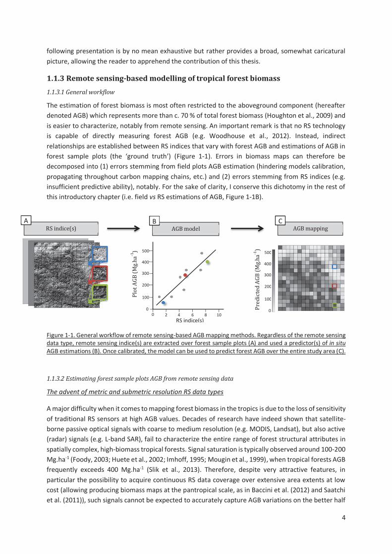
The estimation of forest biomass is most often restricted to the aboveground component (hereafter
denoted AGB) which represents more than c. 70 % of total forest biomass (Houghton et al., 2009) and
is easier to characterize, notably from remote sensing. An important remark is that no RS technology
is capable of directly measuring forest AGB (e.g. Woodhouse et al., 2012). Instead, indirect
relationships are established between RS indices that vary with forest AGB and estimations of AGB in
forest sample plots (the ‘ground truth’) (Figure 1-1). Errors in biomass maps can therefore be
decomposed into (1) errors stemming from field plots AGB estimation (hindering models calibration,
propagating throughout carbon mapping chains, etc.) and (2) errors stemming from RS indices (e.g.
insufficient predictive ability), notably. For the sake of clarity, I conserve this dichotomy in the rest of
this introductory chapter (i.e. field vs RS estimations of AGB, Figure 1-1B).
Figure 1-1. General workflow of remote sensing-based AGB mapping methods. Regardless of the remote sensing data type, remote sensing indice(s) are extracted over forest sample plots (A) and used a predictor(s) of in situ AGB estimations (B). Once calibrated, the model can be used to predict forest AGB over the entire study area (C).
1.1.3.2 Estimating forest sample plots AGB from remote sensing data
The advent of metric and submetric resolution RS data types
A major difficulty when it comes to mapping forest biomass in the tropics is due to the loss of sensitivity
of traditional RS sensors at high AGB values. Decades of research have indeed shown that satellite-
borne passive optical signals with coarse to medium resolution (e.g. MODIS, Landsat), but also active
(radar) signals (e.g. L-band SAR), fail to characterize the entire range of forest structural attributes in
spatially complex, high-biomass tropical forests. Signal saturation is typically observed around 100-200
Mg.ha-1 (Foody, 2003; Huete et al., 2002; Imhoff, 1995; Mougin et al., 1999), when tropical forests AGB
frequently exceeds 400 Mg.ha-1 (Slik et al., 2013). Therefore, despite very attractive features, in
particular the possibility to acquire continuous RS data coverage over extensive area extents at low
cost (allowing producing biomass maps at the pantropical scale, as in Baccini et al. (2012) and Saatchi
et al. (2011)), such signals cannot be expected to accurately capture AGB variations on the better half
RS indice(s) AGB mapping
Pre
dic
ted
AG
B (
Mg
.ha
-1)
AGB model
Plo
t A
GB
(M
g.h
a-1
)
RS indice(s) 0 2 4 6 8 10
100
200
300
400
500
0
100
200
300
400
500
0
A B C
5
of the tropical forest AGB gradient. The development of reliable, non-saturating AGB mapping
methods in the tropical context remains an active field of research.
Since the early 2000s, Light Detection And Ranging (LiDAR) technology has become increasingly
popular in this regard. Aircraft-based LiDAR systems provide information on forest structure with a
ground resolution of 5 m to 50 cm (or less), depending on system characteristics. Importantly, LiDAR
is an active signal that penetrates forest canopy down to the ground surface, generating a detailed
description of forest three-dimensional (3D) structure. From this extremely rich data type (which often
allows identifying individual trees and large branches with the naked eye), a common approach is to
aggregate the information into one or several forest height indices that can be related to plot level
AGB estimates (e.g. Asner et al., 2011; Véga et al., 2015). A growing body of literature suggests that
aerial LiDAR indices allow detecting the full gradient of tropical forest AGB (no saturation) with a
relatively high precision (10-20 % error, Zolkos et al., 2013). However, airborne data acquisition
campaigns are costly and sometimes unfeasible in certain tropical countries for logistical and political
reasons, hampering the use of aerial LiDAR for routine, large scale monitoring of forest AGB.
Another type of RS data that could prove useful in the carbon monitoring context and yet has largely
been under-exploited is satellite-borne Very High Spatial Resolution (VHSR, with pixel size ≤ 1 m²)
optical images. Much like LiDAR (although in two dimensions), the spatial resolution of these optical
images allows one to visually identify individual (canopy) trees in the image. In contrast with LiDAR
however, the optical signal is passive, therefore forests AGB retrieval cannot be based on forest height
proxies. Instead, the two-dimensional information on canopy structure may be exploited using an
analysis of canopy texture properties. The Fourier Texture Ordination (FOTO) method for instance
(which rationale and previous case studies are presented in chapter 4) have shown promising results
for the retrieval of classical stand structure parameters (e.g. basal area, mean tree diameter) and AGB
in high-biomass tropical forests (Couteron et al., 2005; Proisy et al., 2007). Biophysical mechanisms
governing relationships between canopy texture features and forest structure are, however, not fully
understood. This is an important knowledge gap as it prevents to move from local applications (i.e.
statistical relationships established on a single forest type, over a few hundred km²) to larger scales
(i.e. several forest types, over several thousands km²).
The prospects of coupling 3D plant models and radiative transfer models
Deepening our understanding of how forest 3D structure controls canopy texture properties, how
texture-based indices translate back into standard stand structure parameters (including AGB) and
how those relations vary across forest ecosystems and spatial scales is made difficult by the absence
of a sufficiently large dataset featuring both field inventories and VHSR data. Besides, sun-sensor
geometry (e.g. sun elevation angle) at the time of satellite image acquisition influences canopy texture
properties (e.g. by modifying the amount and spatial distribution of shadows on the canopy) (Barbier
et al., 2011), any empirical approach of the problem must therefore account for this phenomenon by
disentangling instrumental perturbation from the effect of forest stand structure on canopy texture.
On a small set of VHSR images, this issue is typically bypassed by inter-calibrating texture-based indices
when images partly overlap (as in Bastin et al., 2014) or analyzing images acquired in similar acquisition
angles, but restricting image acquisition angles to relatively narrow range of values is an important
constraint for image providers and can hardly be envisaged, in practice, for large images sets. A
potential workaround is to use a simulation approach (Figure 1-2) coupling (i) a 3D forest simulation
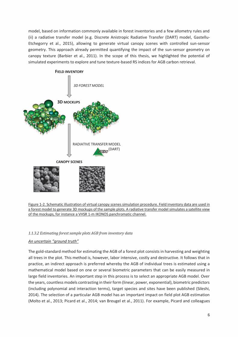
6
model, based on information commonly available in forest inventories and a few allometry rules and
(ii) a radiative transfer model (e.g. Discrete Anistropic Radiative Transfer (DART) model, Gastellu-
Etchegorry et al., 2015), allowing to generate virtual canopy scenes with controlled sun-sensor
geometry. This approach already permitted quantifying the impact of the sun-sensor geometry on
canopy texture (Barbier et al., 2011). In the scope of this thesis, we highlighted the potential of
simulated experiments to explore and tune texture-based RS indices for AGB carbon retrieval.
Figure 1-2. Schematic illustration of virtual canopy scenes simulation procedure. Field inventory data are used in a forest model to generate 3D mockups of the sample plots. A radiative transfer model simulates a satellite view of the mockups, for instance a VHSR 1-m IKONOS panchromatic channel.
1.1.3.2 Estimating forest sample plots AGB from inventory data
An uncertain “ground truth”
The gold-standard method for estimating the AGB of a forest plot consists in harvesting and weighting
all trees in the plot. This method is, however, labor intensive, costly and destructive. It follows that in
practice, an indirect approach is preferred whereby the AGB of individual trees is estimated using a
mathematical model based on one or several biometric parameters that can be easily measured in
large field inventories. An important step in this process is to select an appropriate AGB model. Over
the years, countless models contrasting in their form (linear, power, exponential), biometric predictors
(including polynomial and interaction terms), target species and sites have been published (Sileshi,
2014). The selection of a particular AGB model has an important impact on field plot AGB estimation
(Molto et al., 2013; Picard et al., 2014; van Breugel et al., 2011). For example, Picard and colleagues
3D MOCKUPS
CANOPY SCENES
3D FOREST MODEL
RADIATIVE TRANSFER MODEL (DART)
FIELD INVENTORY
7
(2015) obtained AGB estimations varying by a factor of nearly two when comparing seven seemingly
appropriate AGB models on a 9-ha forest plot of Democratic Republic of Congo. Disagreements of AGB
models on levels and variation pattern of AGB across forest plots naturally limits the accuracy with
which RS methods can predict spatial variations of AGB (Ahmed et al., 2013; Mitchard et al., 2013).
The pantropical biomass model
Following the seminal study of Brown (1997), J. Chave made important contributions toward
standardizing the way we estimate trees AGB across the tropics by developing a pantropical approach
(Chave et al., 2014, 2005). This approach has major premises that are worth being mentioned. First,
pantropical AGB models are mixed-species models. Because tree species diversity in tropical forests is
generally comprised between 100 and 300 species per ha (De Oliveira and Mori, 1999; Turner, 2001),
developing species-specific equations as it is done in temperate forests (e.g. Brown and Schroeder,
1999) is currently unrealistic. Second, the geographical span of models validity englobes the entire
tropics. This feature is particularly attractive because in most instances, as in the study of Picard and
colleagues (2015), one does not have a priori knowledge on the relevance of a particular AGB model.
Provided that AGB predictions from a pantropical model do not present systematic bias pattern at the
local level (e.g. associated to specific stand species composition or environmental characteristics),
using a single AGB model for all plots in large scale RS studies would provide a more consistent and
transparent synthesis of spatial AGB variations derived from field data. Making accurate predictions of
tree AGB regardless of species and geographic locations requires accounting for biometric predictors
that reflect inter- tree AGB variation with sufficient generality and yet capture systematic trends on
how tree AGB varies with tree size along ontogeny, across species and in space. Among the models
proposed by Chave et al. (2014), the most powerful one (hereafter referred to as the pantropical AGB
model) combines trunk diameter at breast height (D in cm), tree height (H in m) and wood specific
gravity (ρ in g.cm-3) in a compound variable related to AGB (in kg) through a power law of parameters
% and & (eq. 1).
'() = % " *!+ " # " $,- (eq. 1)
Equation 1 was calibrated on a destructive dataset containing more than 4000 trees from 58 sampling
sites distributed across the pantropical belt. Chave and colleagues conducted a nested analysis of
variance on model residuals (i.e. sampling site within forest type). The forest type factor (i.e. dry, moist,
wet) accounted for less than 1 % of residuals variability, indicating that the AGB - D+ " H " .
relationship holds well across broad environmental conditions. Sampling sites accounted for only c. 20
% of residuals variability, and adjusting equation 1 on data subsets from each site led to an average
uncertainty on tree level predictions only slightly lower than with the pantropical model (i.e. c. 47 %
vs c. 56 %, respectively) (Chave et al., 2014). These results provide a strong support for a pantropical
approach of tree AGB modelling.
The pantropical model error on individual tree AGB prediction is huge (about 50 %), but this error
levels-off when randomly accumulating trees, because positive and negative individual errors
compensate (Chave et al., 2004; Picard et al., 2014). Assuming 50 % random prediction error on each
tree, the prediction error on the AGB of a typical 1 ha forest plot should range between 5 and 10 % of
the mean (Chave et al., 2014). High individual error stems from important AGB variations between
trees of similar DBH, H and . (Molto et al., 2013) and could be reduced by including additional
predictors in the model (e.g. crown diameter, Goodman et al., 2014), notably to increase the precision
8
of AGB predictions on plots of small size (e.g. < 1 ha). A more important issue is that the pantropical
model systematically underestimates the AGB of large trees (c. 30 Mg) by c. 20 %. Given the
importance of large trees for forest AGB stock (Bastin et al., 2015; Slik et al., 2013) and stock change
(Stephenson et al., 2014), understanding the origin and consequences of this bias is of utmost concern.
Allometric theory of tree branching networks
Tree AGB models lie on the concept of ‘allometry’. The term allometry was coined by Huxley and
Teissier (1936) ‘‘to denote growth of a part [of an organism] at a different rate from that of [the
organism] body as a whole’’. The simplest and most widespread type of tree AGB allometric model is
a simple, bivariate relationship based on D. In such a model, the growth of whole tree AGB (“the body”)
is assessed through the growth of D (“the part”). Because growth data often fit particularly well to a
straight line when plotted in logarithmic units (Stevens, 2009), the dominating mathematical function
used to model allometries is a power function (as in equation 1). Perhaps the most important feature
of the power model form in the context of allometry, and in our case AGB allometry, is that it implies
a constant scaling (&) of AGB and D (or !+ " # " $ in the pantropical model) across the whole ontogenic
development of the organism.
On the one hand, scale-invariance (or self-similarity) properties has been documented for many
animals and plants traits (e.g. West et al., 1997) and is thought to reflect universal principles governing
biological systems (e.g. Marquet, 2005). Several allometric theories, such as the Metabolic Theory of
Ecology (MTE, West et al., 1999, 1997), derive universal scaling laws (i.e. simple power model
allometries) between plants dimensions from lower-level assumptions on plants branching structure,
and thus support simple power-law allometries.
On the other hand, this scale-invariance hypothesis in the relative growth of organisms’ parts (or
between a part and the body as a whole) has been intensely criticized (e.g. Nijhout and German, 2012).
Some consider that the power model form is fundamentally empirical and lacks biological foundations.
For example, Nijhout and German (2012) pointed out that an implicit assumption in the power model
form is that all body parts begin and end their growth at the same time during ontogeny. In the case
of trees, it is commonly accepted that the growth in H slows down and eventually stops long before
the growth in D. Empirically, several tree dimensions such as tree height or tree crown diameter show
a constant scaling (&) with D only on a finite D range (Antin et al., 2013; Blanchard et al., 2016), leading
Picard et al. (2015) to stress that since “many non-power models can bring nearly constant scaling
across a wide range of scale, simple allometry may be confused with complex allometry” (“complex
allometry” in this statement refers to a model with multiple predictors that does not necessarily take
the form of a power function). Whether relationships between tree AGB and D or !+ " # " $ conform
to power function remains a pending question.
1.2 Research objectives
The general objective of this thesis is to use information on the structure and spatial organization of
canopy trees to improve our ability to model forest AGB from field and RS data.
Our analyses are restricted to two approaches that were deemed promising: the pantropical approach
for the estimation of AGB at the tree and plot level (i.e. from field data) and the canopy texture
approach for the detection and extrapolation of field-derived AGB estimations via RS data.
9
A first part of this work seeks to increase our understanding of the pantropical model error and
propose ways to mitigate this error. In particular, the compound predictor variable of the pantropical
model (!+ " # " $) does not allow capturing between-tree variations in relative crown dimensions,
while crown allometries varies between species, along tree ontogeny and environmental gradients
(e.g. Banin et al., 2012; Cannell, 1984; Poorter et al., 2006). We thus:
(i) Assess the contribution of crown mass variation to the pantropical model error, either at the tree
level or when propagated to the plot level;
(ii) Propose a new operational strategy to explicitly take crown mass variation into account in
pantropical AGB models.
We further used the predictions of the MTE on branch scaling properties as a point-of-entry to
investigate the relevance of the power model form in AGB allometries. Specifically, we:
(iii) Test whether large trees branching structure conform to the predictions of the MTE.
A second part of the thesis focuses on assessing and improving the potential of a canopy texture-based
RS method (FOTO) to retrieve tropical forest AGB. Here, a major objective was to:
(iv) Stabilize the texture-structure relationship across contrasted forest types from different regions of
the world.
1.3 A pantropical approach
This thesis is based on two types of field data: (i) destructive measurements at the tree level and (ii)
forest inventories at plot level. In this section, I briefly explain where the data I assembled came from
and what the datasets are composed of.
1.3.1 Study areas and datasets
Central Africa
Core datasets of this work (at both tree- and plot-level) come from about five years of field data
collection campaigns in central Africa (Cameroon, Gabon, Democratic Republic of Congo) carried out
by the Institut de Recherche pour le Développement (IRD) in collaboration with the Ecole Normale
Supérieure of Yaoundé I (LaBosystE, ENS, Université de Yaoundé I), the Missouri Botanical Garden
(MBG) and the Université Libre de Kisangani (UniKis). During the two years preceding my thesis and
during the thesis itself, I participated to the establishment of nearly 80 1-ha forest inventory plots, the
bulk of which being located in south-eastern Cameroon (c. 50 %, left panel in Figure 1-3). Forests in
this region have been described as a transitional type between evergreen and deciduous forests
(Letouzey, 1985) and expand across the borders of neighboring countries. From a structural point of
view, these forests can be described as forests mosaics that notably include patches of mixed, closed-
canopy, semi-deciduous stands, open-canopy Marantaceae stands and monodominant
Gilbertiodendron dewevrei stands. The diversity of stands structural profiles, from which contrasted
canopy textures emerge (illustrated in Figure 1-3), justifies our interest in this region. Forests of south-
eastern Cameroon are also particularly rich in tall trees and stock relatively high biomass densities
10
(Fayolle et al., 2016), and several logging companies are established in the region. Through a
collaboration with the Alpicam company, we assembled a large destructive dataset on trees
dimensions and AGB (77 trees).
Additional study areas
In the scope of this thesis, I investigate broad biophysical relationships, be it at the tree level in biomass
allometry models or at the stand levels in canopy texture-based AGB models. In order to increase the
robustness of the results, I compiled additional data from the literature, collaborating institutions or
peer researchers (right panel on Figure 1-3).
The sets of 1 ha forest inventories from IRD and collaborators field work in central Africa were
complemented with 28 1-ha plots from a forest-savanna mosaic in Republic Democratic of Congo (from
Bastin et al., 2014), a 50 ha plots located in the Atlantic evergreen forests of western Cameroon (from
Chuyong et al., 2004), 15 and 22 1-ha plots in evergreen and semi-deciduous forests of the Western
Ghats of India (from Ploton et al., 2011 and Pargal et al., submitted) and 16 plots covering 85 ha of
evergreen forests at Paracou, French Guiana (from Vincent et al., 2012). In total, texture analyses were
based on 279 ha of forest inventory distributed on 3 continents.
To the 77 trees destructively sampled in south-eastern Cameroon, I added 132 trees from a semi-
deciduous forest of the same region (from Fayolle et al., 2013), 99 trees sampled in a semi-deciduous
forest of Gabon (from Ngomanda et al., 2014), 29 trees sampled in an evergreen forest of Ghana (from
Henry et al., 2010), 285 trees sampled in a dry-to-wet forest types gradient in Madagascar (from
Vieilledent et al., 2012) and 51 trees sampled in an evergreen forest of Peru (from Goodman et al.,
2014). The total destructive dataset (n=673) thus comprises trees from 6 sites distributed in five
tropical countries (right panel in Figure 1-3).
Figure 1-3. Distribution of datasets across the tropics. Dots and triangles represent tree-level destructive datasets and field plot inventories, respectively. Red color indicates that data have been collected by IRD. Blue color indicates that data were compiled from literature, collaborating institutions or shared by the peer researchers.
CAMEROON
GABON
11
Figure 1-4. VHSR satellite image (GeoEye sensor) covering a typical forest mosaic from semi-deciduous forests of south-eastern Cameroon. Patches of Gilbertiodendron dewevrei (black square), mixed closed-canopy stands (red square) and open-canopy Marantaceae stands closely co-occur.
1.3.2 Sampling strategy and data description
Tree-level destructive data
Large trees exhibits the largest AGB variability at a given D and H while being insufficiently represented
in biomass destructive datasets (Chave et al., 2005), probably because of the disproportionate amount
of work that the biomass estimation of a large tropical canopy tree represents. To fill this gap, we
exclusively targeted very large canopy trees in our field work protocol. This unique dataset, which was
incorporated in the latest pantropical database (Chave et al. 2014), contains 17 out of the 30 world’s
heaviest sampled tropical trees. For a typical tree, we measured the trunk diameter D, the tree height
H and two perpendicular crown diameters before the tree was felled. After felling, tree biomass was
estimated by combining direct measurements, indirect measurements and allometries. Direct
measurements (i.e. weightings) were made on branches of varying sizes, to build an allometry relating
branch diameter to biomass. We estimated the volume of the largest tree components (i.e. trunk and
branches with diameter > 20 cm) by measuring diameters and lengths of approximately 2-m and 1-m
long subsections along the trunk and branches, respectively. Biomass values were obtained by
multiplying volumes by wood density estimates, derived from wood samples. The biomass of branches
with D ≤ 20 cm was obtained with species-specific biomass allometries. A detailed description of the
field protocol is provided in the supplementary material of chapter 2. An important feature of this
dataset is that it contains a description of the crown geometry (from diameter and length
measurements) and topology (from the identification of branching points), allowing to reconstruct the
tree branching network (up to a branch diameter of c. 20 cm) in 3D and explore allometries and scaling
properties at the branch level.
Destructive data compiled from other studies were obtained by direct biomass measurement, I refer
the reader to the publications associated to each dataset for more details. Importantly, I only
considered datasets providing enough information to distinguish trunk from crown biomass (rather
than ones providing a single total tree biomass estimate).
0
10
0
20
0 m
12
Plot level data
Apart for plots at Paracou (85 ha) and Korup (50 ha), the sampling strategy at all sites was designed to
optimize canopy texture analyses from VHSR optical images. In essence, 1 ha plots were distributed
over a few hundred square kilometers (the typical footprint of a VHSR image) so to capture local
diversity of forest stand types and ages. Measurement protocols deployed in central Africa, India and
French Guiana were similar and consisted in describing the structure and composition of forest stands
for all trees with D ≥ 10 cm. In addition to tree diameter at breast height (D), the description of stands
structure included measurements of total tree height (H), trunk height (Ht) and crown diameter (Cd)
on a subset of trees per plot (typically c. 50), to document local trees allometries. The identification of
tree species allows retrieving species-level wood density estimates (ρ) from global databases (e.g.
Zanne et al., 2009) and compute plots AGB with the reference pantropical biomass model (Chave et
al., 2014).
1.4 Thesis outline
The thesis is structured into six chapters. The current chapter briefly depicts the scientific context and
motivations of my doctoral study. It also includes the thesis research objectives, a description of the
datasets and the thesis structure. A last section lists the publications I authored or co-authored on
research topics related to the thesis subject.
In Chapter 2, I investigate how variations in tree form, with a particular focus on crown dimensions,
influence the predictions (and error) of the pantropical biomass model. The analyses are based on the
largest destructive dataset available to date that features information on tropical tree crown mass.
After pinpointing the source of bias in the pantropical model, I propose an alternative model functional
form. An original method for propagating tree biomass estimation error at the plot level is developed
and highlights an interaction between forest structure and biomass model error, a source of
uncertainty largely overlooked. This study was partly published in the journal Biogeosciences.
In Chapter 3, I further explore the structural properties of large trees crowns that could explain the
deviation between large trees biomass and the mathematical power form of the pantropical biomass
model. An empirical assessment of MTE’s theoretical branch allometry is provided. A manuscript is in
preparation from these results for the journal Trees – Structure and Function.
Chapter 4 presents the FOTO method, i.e. a remote sensing approach to retrieve forest structure and
biomass gradients from canopy texture features. I give a concise description of how the method works
and the basic rationale behind it. Further, I provide a synthetic overview of the results obtained in
separate empirical FOTO case studies on diverse forest ecosystems and from various remote sensing
data types. This synthesis highlights methodological limits hindering the development of FOTO as a
broad-scale, operational forest biomass monitoring method. This chapter was partly published in a
book entitled Treetops at Risk (Springer).
Chapter 5 builds upon the synthesis in chapter 4. A simulation procedure is used, which includes the
representation of forest sample plots as three-dimensional mockups and the generation of virtual
mockup canopy scenes. Simulated canopy scenes allow testing how the relation between texture
features and stand biomass varies across forest types in a single, unified analysis frame (as opposed to
previous empirical studies). The major limits identified in chapter 4 are addressed by complementing
13
FOTO texture with additional descriptors of forest stand structure, notably derived from lacunarity
analysis. A ‘generalized’ biomass prediction model based on a combination of texture metrics is
proposed, opening new perspectives for biomass retrieval from canopy texture at large scale. Part of
these results was submitted for publication in Remote Sensing of Environment.
Finally, Chapter 6 presents the overall thesis discussion, focusing on the main contributions, limits and
perspectives of this work.
1.5 List of (co-)publications
Estimation of biomass in forest sample plots
· Ploton, P., Barbier, N., Takoudjou Momo, S., Réjou-Méchain, M., Boyemba Bosela, F., Chuyong, G., Dauby, G., Droissart, V., Fayolle,
A., Goodman, R.C., Henry, M., Kamdem, N.G., Mukirania, J.K., Kenfack, D., Libalah, M., Ngomanda, A., Rossi, V., Sonké, B., Texier, N.,
Thomas, D., Zebaze, D., Couteron, P., Berger, U., Pélissier, R., 2016. Closing a gap in tropical forest biomass estimation: taking crown
mass variation into account in pantropical allometries. Biogeosciences 13, 1571–1585. doi:10.5194/bg-13-1571-2016
· Ploton, P., Barbier, N., Couteron, P., Momo, S.T., Griffon, S., Sonké, B., Uta, B., Pélissier, R. Assessing Da Vinci’s rule on large tropical
tree crowns of contrasted architectures : evidence for area-increasing branching. In preparation for Trees – Structure and Function.
· Picard, N., Rutishauser, E., Ploton, P., Ngomanda, A., Henry, M., 2015. Should tree biomass allometry be restricted to power models?
For. Ecol. Manag. 353, 156–163. doi:10.1016/j.foreco.2015.05.035
· Chave, J., Réjou-Méchain, M., Búrquez, A., Chidumayo, E., Colgan, M.S., Delitti, W.B.C., Duque, A., Eid, T., Fearnside, P.M., Goodman,
R.C., Henry, M., Martínez-Yrízar, A., Mugasha, W.A., Muller-Landau, H.C., Mencuccini, M., Nelson, B.W., Ngomanda, A., Nogueira,
E.M., Ortiz-Malavassi, E., Pélissier, R., Ploton, P., Ryan, C.M., Saldarriaga, J.G., Vieilledent, G., 2014. Improved allometric models to
estimate the aboveground biomass of tropical trees. Glob. Change Biol. 20, 3177–3190. doi:10.1111/gcb.12629
Rational behind texture-based remote sensing methods
· Bastin, J.-F., Barbier, N., Réjou-Méchain, M., Fayolle, A., Gourlet-Fleury, S., Maniatis, D., de Haulleville, T., Baya, F., Beeckman, H.,
Beina, D., Couteron, P., Chuyong, G., Dauby, G., Doucet, J.-L., Droissart, V., Dufrêne, M., Ewango, C., Gillet, J.F., Gonmadje, C.H., Hart,
T., Kavali, T., Kenfack, D., Libalah, M., Malhi, Y., Makana, J.-R., Pélissier, R., Ploton, P., Serckx, A., Sonké, B., Stevart, T., Thomas, D.W.,
De Cannière, C., Bogaert, J., 2015c. Seeing Central African forests through their largest trees. Sci. Rep. 5, 13156.
doi:10.1038/srep13156
· Blanchard, E., Birnbaum, P., Ibanez, T., Boutreux, T., Antin, C., Ploton, P., Vincent, G., Pouteau, R., Vandrot, H., Hequet, V., 2016.
Contrasted allometries between stem diameter, crown area, and tree height in five tropical biogeographic areas. Trees 1–16.
· Jucker, T., Caspersen, J., Chave, J., Antin, C., Barbier, N., Bongers, F., Dalponte, M., van Ewijk, K.Y., Forrester, D.I., Haeni, M., Higgins,
S.I., Holdaway, R.J., Iida, Y., Lorimer, C., Marshall, P.L., Momo, S., Moncrieff, G.R., Ploton, P., Poorter, L., Rahman, K.A., Schlund, M.,
Sonké, B., Sterck, F.J., Trugman, A.T., Usoltsev, V.A., Vanderwel, M.C., Waldner, P., Wedeux, B.M.M., Wirth, C., Wöll, H., Woods, M.,
Xiang, W., Zimmermann, N.E., Coomes, D.A., 2016. Allometric equations for integrating remote sensing imagery into forest
monitoring programmes. Glob. Change Biol. doi:10.1111/gcb.13388
Estimation of biomass from canopy texture features
· Ploton, P., Pélissier, R., Barbier, N., Proisy, C., Ramesh, B.R., Couteron, P., 2013. Canopy texture analysis for large-scale assessments
of tropical forest stand structure and biomass, in: Treetops at Risk. Springer, pp. 237–245.
· Ploton, P., Barbier, N., Couteron, P., Ayyappan, N., Antin, C.M., Bastin, J.-F., Chuyong, G., Dauby, G., Droissart, V., Gastellu-Etchegorry,
J.-P., Kamdem, N.G., Kenfack, D., Libalah, M., Momo, S., Pargal, S., Proisy, C., Sonké, B., Texier, N., Thomas, D., Zebaze, D., Verley, P.,
Vincent, G., Berger, U., Pélissier, R. Combining canopy texture metrics from optical data to retrieve tropical forest aboveground
biomass in complex forest mosaics. Submitted to Remote Sensing of Environment.
· Ploton, P., Pélissier, R., Proisy, C., Flavenot, T., Barbier, N., Rai, S.N., Couteron, P., 2012. Assessing aboveground tropical forest
biomass using Google Earth canopy images. Ecol. Appl. 22, 993–1003. doi:10.1890/11-1606.1
· Couteron, P., Barbier, N., Deblauwe, V., Pélissier, R., Ploton, P., 2015. Texture Analysis of Very High Spatial Resolution Optical Images
as a Way to Monitor Vegetation and Forest Biomass in the Tropics. Multi-Scale For. Biomass Assess. Monit. Hindu Kush Himal. Reg.
Geospatial Perspect. 157.
14
1.6 References
Ahmed, R., Siqueira, P., Hensley, S., Bergen, K., 2013. Uncertainty of Forest Biomass Estimates in North Temperate Forests Due to Allometry: Implications for Remote Sensing. Remote Sens. 5, 3007–
3036. doi:10.3390/rs5063007 Antin, C., Pélissier, R., Vincent, G., Couteron, P., 2013. Crown allometries are less responsive than stem
allometry to tree size and habitat variations in an Indian monsoon forest. Trees 27, 1485–1495. doi:10.1007/s00468-013-0896-7
Asner, G.P., Mascaro, J., Muller-Landau, H.C., Vieilledent, G., Vaudry, R., Rasamoelina, M., Hall, J.S., Breugel, M. van, 2011. A universal airborne LiDAR approach for tropical forest carbon mapping. Oecologia 168, 1147–1160. doi:10.1007/s00442-011-2165-z
Baccini, A., Goetz, S.J., Walker, W.S., Laporte, N.T., Sun, M., Sulla-Menashe, D., Hackler, J., Beck, P.S.A., Dubayah, R., Friedl, M.A., 2012. Estimated carbon dioxide emissions from tropical deforestation improved by carbon-density maps. Nat. Clim. Change 2, 182–185.
Banin, L., Feldpausch, T.R., Phillips, O.L., Baker, T.R., Lloyd, J., Affum-Baffoe, K., Arets, E.J.M.M., Berry, N.J., Bradford, M., Brienen, R.J.W., Davies, S., Drescher, M., Higuchi, N., Hilbert, D.W., Hladik, A., Iida, Y., Salim, K.A., Kassim, A.R., King, D.A., Lopez-Gonzalez, G., Metcalfe, D., Nilus, R., Peh, K.S.-H., Reitsma, J.M., Sonké, B., Taedoumg, H., Tan, S., White, L., Wöll, H., Lewis, S.L., 2012. What controls tropical forest architecture? Testing environmental, structural and floristic drivers. Glob. Ecol. Biogeogr. 21, 1179–1190. doi:10.1111/j.1466-8238.2012.00778.x
Barbier, N., Proisy, C., Véga, C., Sabatier, D., Couteron, P., 2011. Bidirectional texture function of high resolution optical images of tropical forest: An approach using LiDAR hillshade simulations. Remote Sens. Environ. 115, 167–179.
Bastin, J.-F., Barbier, N., Couteron, P., Adams, B., Shapiro, A., Bogaert, J., De Cannière, C., 2014. Aboveground biomass mapping of African forest mosaics using canopy texture analysis: toward a regional approach. Ecol. Appl. 24, 1984–2001.
Bastin, J.-F., Barbier, N., Réjou-Méchain, M., Fayolle, A., Gourlet-Fleury, S., Maniatis, D., de Haulleville, T., Baya, F., Beeckman, H., Beina, D., 2015. Seeing Central African forests through their largest trees. Sci. Rep. 5. doi:doi:10.1038/srep13156
Blanchard, E., Birnbaum, P., Ibanez, T., Boutreux, T., Antin, C., Ploton, P., Vincent, G., Pouteau, R., Vandrot, H., Hequet, V., 2016. Contrasted allometries between stem diameter, crown area, and tree height in five tropical biogeographic areas. Trees 1–16.
Brown, S., 1997. Estimating biomass and biomass change of tropical forests: a primer, UN FAO Forestry Paper 134. Food and Agriculture Organization, Rome.
Brown, S.L., Schroeder, P.E., 1999. Spatial patterns of aboveground production and mortality of woody biomass for eastern US forests. Ecol. Appl. 9, 968–980.
Cannell, M.G.R., 1984. Woody biomass of forest stands. For. Ecol. Manag. 8, 299–312. doi:10.1016/0378-1127(84)90062-8
Chave, J., Andalo, C., Brown, S., Cairns, M.A., Chambers, J.Q., Eamus, D., Fölster, H., Fromard, F., Higuchi, N., Kira, T., Lescure, J.-P., Nelson, B.W., Ogawa, H., Puig, H., Riéra, B., Yamakura, T., 2005. Tree allometry and improved estimation of carbon stocks and balance in tropical forests. Oecologia 145, 87–99. doi:10.1007/s00442-005-0100-x
Chave, J., Condit, R., Aguilar, S., Hernandez, A., Lao, S., Perez, R., 2004. Error propagation and scaling for tropical forest biomass estimates. Philos. Trans. R. Soc. Lond. B. Biol. Sci. 359, 409–420. doi:10.1098/rstb.2003.1425
Chave, J., Réjou-Méchain, M., Búrquez, A., Chidumayo, E., Colgan, M.S., Delitti, W.B.C., Duque, A., Eid, T., Fearnside, P.M., Goodman, R.C., Henry, M., Martínez-Yrízar, A., Mugasha, W.A., Muller-Landau, H.C., Mencuccini, M., Nelson, B.W., Ngomanda, A., Nogueira, E.M., Ortiz-Malavassi, E., Pélissier, R., Ploton, P., Ryan, C.M., Saldarriaga, J.G., Vieilledent, G., 2014. Improved
15
allometric models to estimate the aboveground biomass of tropical trees. Glob. Change Biol. 20, 3177–3190. doi:10.1111/gcb.12629
Chuyong, G.B., Condit, R., Kenfack, D., Losos, E.C., Moses, S.N., Songwe, N.C., Thomas, D.W., 2004. Korup forest dynamics plot, Cameroon. Trop. For. Divers. Dynamism 506–516.
Couteron, P., Pelissier, R., Nicolini, E.A., Paget, D., 2005. Predicting tropical forest stand structure parameters from Fourier transform of very high-resolution remotely sensed canopy images. J.
Appl. Ecol. 42, 1121–1128. De Oliveira, A.A., Mori, S.A., 1999. A central Amazonian terra firme forest. I. High tree species richness
on poor soils. Biodivers. Conserv. 8, 1219–1244. De Sy, V., Herold, M., Achard, F., Asner, G.P., Held, A., Kellndorfer, J., Verbesselt, J., 2012. Synergies of
multiple remote sensing data sources for REDD+ monitoring. Curr. Opin. Environ. Sustain. 4, 696–706.
Eggleston, H.S., Buendia, L., Miwa, K., Ngara, T., Tanabe, K., 2006. 2006 IPCC guidelines for national greenhouse gas inventories. Agriculture, Forestry and Other Land Use. Inst. Glob. Environ. Strateg. IGES Behalf Intergov. Panel Clim. Change IPCC Hayama Jpn. 4.
FAO, 2010. Global Forest Resources Assessment 2010 (FAO Forestry Paper No. 163). Food and Agriculture Organization of the United Nations, Rome.
Fayolle, A., Doucet, J.-L., Gillet, J.-F., Bourland, N., Lejeune, P., 2013. Tree allometry in Central Africa: Testing the validity of pantropical multi-species allometric equations for estimating biomass and carbon stocks. For. Ecol. Manag. 305, 29–37. doi:10.1016/j.foreco.2013.05.036
Fayolle, A., Loubota Panzou, G.J., Drouet, T., Swaine, M.D., Bauwens, S., Vleminckx, J., Biwole, A., Lejeune, P., Doucet, J.-L., 2016. Taller trees, denser stands and greater biomass in semi-deciduous than in evergreen lowland central African forests. For. Ecol. Manag. 374, 42–50. doi:10.1016/j.foreco.2016.04.033
Foody, G.M., 2003. Remote sensing of tropical forest environments: towards the monitoring of environmental resources for sustainable development. Int. J. Remote Sens. 24, 4035–4046.
Gastellu-Etchegorry, J.-P., Yin, T., Lauret, N., Cajgfinger, T., Gregoire, T., Grau, E., Feret, J.-B., Lopes, M., Guilleux, J., Dedieu, G., 2015. Discrete Anisotropic Radiative Transfer (DART 5) for modeling airborne and satellite spectroradiometer and LIDAR acquisitions of natural and urban landscapes. Remote Sens. 7, 1667–1701.
Goodman, R.C., Phillips, O.L., Baker, T.R., 2014. The importance of crown dimensions to improve tropical tree biomass estimates. Ecol. Appl. 24, 680–698.
Gullison, R.E., Frumhoff, P.C., Canadell, J.G., Field, C.B., Nepstad, D.C., Hayhoe, K., Avissar, R., Curran, L.M., Friedlingstein, P., Jones, C.D., Nobre, C., 2007. Tropical Forests and Climate Policy. Science 316, 985–986. doi:10.1126/science.1136163
Henry, M., Besnard, A., Asante, W.A., Eshun, J., Adu-Bredu, S., Valentini, R., Bernoux, M., Saint-André, L., 2010. Wood density, phytomass variations within and among trees, and allometric equations in a tropical rainforest of Africa. For. Ecol. Manag. 260, 1375–1388. doi:10.1016/j.foreco.2010.07.040
Houghton, R.A., 2012. Carbon emissions and the drivers of deforestation and forest degradation in the tropics. Curr. Opin. Environ. Sustain. 4, 597–603.
Houghton, R.A., 2007. Balancing the Global Carbon Budget. Annu Rev Earth Planet Sci 35, 313–347. Houghton, R.A., 2005. Aboveground forest biomass and the global carbon balance. Glob. Change Biol.
11, 945–958. Houghton, R.A., Hall, F., Goetz, S.J., 2009. Importance of biomass in the global carbon cycle. J. Geophys.
Res. Biogeosciences 114. Houghton, R.A., Lawrence, K.T., Hackler, J.L., Brown, S., 2001. The spatial distribution of forest biomass
in the Brazilian Amazon: a comparison of estimates. Glob. Change Biol. 7, 731–746. Huete, A., Didan, K., Miura, T., Rodriguez, E.P., Gao, X., Ferreira, L.G., 2002. Overview of the radiometric
and biophysical performance of the MODIS vegetation indices. Remote Sens. Environ. 83, 195–
213.
16
Huxley, J.S., Teissier, G., 1936. Terminology of Relative Growth. Nature 137, 780–781. doi:10.1038/137780b0
Imhoff, M.L., 1995. Radar backscatter and biomass saturation: ramifications for global biomass inventory. Geosci. Remote Sens. IEEE Trans. On 33, 511–518.
IPCC, 2014. Summary for policymakers, in: Climate Change 2014: Mitigation of Climate Change. Contribution of Working Group III to the Fifth Assessment Report of the Intergovernmental Panel on Climate Change. Cambridge University Press, Cambridge, United Kingdom and New York, NY, USA, pp. 1–30.
Langner, A., Achard, F., Grassi, G., 2014. Can recent pan-tropical biomass maps be used to derive alternative Tier 1 values for reporting REDD+ activities under UNFCCC? Environ. Res. Lett. 9, 124008. doi:10.1088/1748-9326/9/12/124008
Letouzey, R., 1985. Carte phytogéographique du Cameroun. Institut de la recherche agronomique. Marquet, P.A., 2005. Scaling and power-laws in ecological systems. J. Exp. Biol. 208, 1749–1769.
doi:10.1242/jeb.01588 Mattsson, E., Ostwald, M., Wallin, G., Nissanka, S.P., 2016. Heterogeneity and assessment
uncertainties in forest characteristics and biomass carbon stocks: Important considerations for climate mitigation policies. Land Use Policy 59, 84–94. doi:10.1016/j.landusepol.2016.08.026
Mitchard, E.T., Feldpausch, T.R., Brienen, R.J., Lopez-Gonzalez, G., Monteagudo, A., Baker, T.R., Lewis,
S.L., Lloyd, J., Quesada, C.A., Gloor, M., 2014. Markedly divergent estimates of Amazon forest carbon density from ground plots and satellites. Glob. Ecol. Biogeogr. 23, 935–946.
Mitchard, E.T., Saatchi, S.S., Baccini, A., Asner, G.P., Goetz, S.J., Harris, N.L., Brown, S., 2013. Uncertainty in the spatial distribution of tropical forest biomass: a comparison of pan-tropical maps. Carbon Balance Manag. 8, 10. doi:10.1186/1750-0680-8-10
Molto, Q., Rossi, V., Blanc, L., 2013. Error propagation in biomass estimation in tropical forests. Methods Ecol. Evol. 4, 175–183. doi:10.1111/j.2041-210x.2012.00266.x
Morton, D.C., 2016. Forest carbon fluxes: A satellite perspective. Nat. Clim. Change 6, 346–348. doi:10.1038/nclimate2978
Mougin, E., Proisy, C., Marty, G., Fromard, F., Puig, H., Betoulle, J.L., Rudant, J.-P., 1999. Multifrequency and multipolarization radar backscattering from mangrove forests. Geosci. Remote Sens. IEEE Trans. On 37, 94–102.
Ngomanda, A., Engone Obiang, N.L., Lebamba, J., Moundounga Mavouroulou, Q., Gomat, H., Mankou, G.S., Loumeto, J., Midoko Iponga, D., Kossi Ditsouga, F., Zinga Koumba, R., Botsika Bobé, K.H., Mikala Okouyi, C., Nyangadouma, R., Lépengué, N., Mbatchi, B., Picard, N., 2014. Site-specific versus pantropical allometric equations: Which option to estimate the biomass of a moist central African forest? For. Ecol. Manag. 312, 1–9. doi:10.1016/j.foreco.2013.10.029
Nijhout, H.F., German, R.Z., 2012. Developmental Causes of Allometry: New Models and Implications for Phenotypic Plasticity and Evolution. Integr. Comp. Biol. 52, 43–52. doi:10.1093/icb/ics068
Ometto, J.P., Aguiar, A.P., Assis, T., Soler, L., Valle, P., Tejada, G., Lapola, D.M., Meir, P., 2014. Amazon forest biomass density maps: tackling the uncertainty in carbon emission estimates. Clim. Change 124, 545–560.
Pan, Y., Birdsey, R.A., Fang, J., Houghton, R., Kauppi, P.E., Kurz, W.A., Phillips, O.L., Shvidenko, A., Lewis, S.L., Canadell, J.G., 2011. A large and persistent carbon sink in the world’s forests. Science 333,
988–993. Pargal, S., Fararoda, R., Rajashekar, G., Balachandran, N., Réjou-Méchain, M., Barbier, N., Jha, C.S.,
Pélissier, R., Dadhwal, V.K., Couteron, P., n.d. Characterizing aboveground biomass – canopy texture relationships in a landscape of forest mosaic in the Western Ghats of India using very high resolution Cartosat Imagery. Remote Sens.
Picard, N., Bosela, F.B., Rossi, V., 2014. Reducing the error in biomass estimates strongly depends on model selection. Ann. For. Sci. 72, 811–923. doi:10.1007/s13595-014-0434-9
Picard, N., Rutishauser, E., Ploton, P., Ngomanda, A., Henry, M., 2015. Should tree biomass allometry be restricted to power models? For. Ecol. Manag. 353, 156–163. doi:10.1016/j.foreco.2015.05.035
17
Ploton, P., Pélissier, R., Proisy, C., Flavenot, T., Barbier, N., Rai, S.N., Couteron, P., 2012. Assessing aboveground tropical forest biomass using Google Earth canopy images. Ecol. Appl. 22, 993–
1003. doi:10.1890/11-1606.1 Poorter, L., Bongers, L., Bongers, F., 2006. Architecture of 54 moist-forest tree species: traits, trade-
offs, and functional groups. Ecology 87, 1289–1301. doi:10.1890/0012-9658(2006)87[1289:AOMTST]2.0.CO;2
Proisy, C., Couteron, P., Fromard, F., 2007. Predicting and mapping mangrove biomass from canopy grain analysis using Fourier-based textural ordination of IKONOS images. Remote Sens. Environ. 109, 379–392.
Ryan, M.G., Binkley, D., Fownes, J.H., 1997. Age-related decline in forest productivity: pattern and process. Adv. Ecol. Res. 27, 213–262.
Saatchi, S.S., Harris, N.L., Brown, S., Lefsky, M., Mitchard, E.T., Salas, W., Zutta, B.R., Buermann, W., Lewis, S.L., Hagen, S., 2011. Benchmark map of forest carbon stocks in tropical regions across three continents. Proc. Natl. Acad. Sci. 108, 9899–9904.
Sileshi, G.W., 2014. A critical review of forest biomass estimation models, common mistakes and corrective measures. For. Ecol. Manag. 329, 237–254. doi:10.1016/j.foreco.2014.06.026
Slik, J.W., Paoli, G., McGuire, K., Amaral, I., Barroso, J., Bastian, M., Blanc, L., Bongers, F., Boundja, P., Clark, C., 2013. Large trees drive forest aboveground biomass variation in moist lowland forests across the tropics. Glob. Ecol. Biogeogr. 22, 1261–1271.
Stephenson, N.L., Das, A.J., Condit, R., Russo, S.E., Baker, P.J., Beckman, N.G., Coomes, D.A., Lines, E.R., Morris, W.K., Rüger, N., Álvarez, E., Blundo, C., Bunyavejchewin, S., Chuyong, G., Davies, S.J., Duque, Á., Ewango, C.N., Flores, O., Franklin, J.F., Grau, H.R., Hao, Z., Harmon, M.E., Hubbell, S.P., Kenfack, D., Lin, Y., Makana, J.-R., Malizia, A., Malizia, L.R., Pabst, R.J., Pongpattananurak, N., Su, S.-H., Sun, I.-F., Tan, S., Thomas, D., van Mantgem, P.J., Wang, X., Wiser, S.K., Zavala, M.A., 2014. Rate of tree carbon accumulation increases continuously with tree size. Nature advance online publication. doi:10.1038/nature12914
Stevens, C.F., 2009. Darwin and Huxley revisited: the origin of allometry. J. Biol. 8, 1. Turner, I.M., 2001. The ecology of trees in the tropical rain forest. Cambridge University Press. UNFCCC, 2007. Reducing Emissions From Deforestation in Developing Countries: Approaches to
Stimulate Action. van Breugel, M., Ransijn, J., Craven, D., Bongers, F., Hall, J.S., 2011. Estimating carbon stock in
secondary forests: Decisions and uncertainties associated with allometric biomass models. For. Ecol. Manag. 262, 1648–1657. doi:10.1016/j.foreco.2011.07.018
Van der Werf, G.R., Morton, D.C., DeFries, R.S., Olivier, J.G., Kasibhatla, P.S., Jackson, R.B., Collatz, G.J., Randerson, J.T., 2009. CO2 emissions from forest loss. Nat. Geosci. 2, 737–738.
Véga, C., Vepakomma, U., Morel, J., Bader, J.-L., Rajashekar, G., Jha, C.S., Ferêt, J., Proisy, C., Pélissier, R., Dadhwal, V.K., 2015. Aboveground-Biomass Estimation of a Complex Tropical Forest in India Using Lidar. Remote Sens. 7, 10607–10625.
Vieilledent, G., Vaudry, R., Andriamanohisoa, S.F., Rakotonarivo, O.S., Randrianasolo, H.Z., Razafindrabe, H.N., Rakotoarivony, C.B., Ebeling, J., Rasamoelina, M., 2012. A universal approach to estimate biomass and carbon stock in tropical forests using generic allometric models. Ecol. Appl. 22, 572–583.
Vincent, G., Sabatier, D., Blanc, L., Chave, J., Weissenbacher, E., Pélissier, R., Fonty, E., Molino, J.-F., Couteron, P., 2012. Accuracy of small footprint airborne LiDAR in its predictions of tropical moist forest stand structure. Remote Sens. Environ. 125, 23–33.
West, G.B., Brown, J.H., Enquist, B.J., 1999. A general model for the structure and allometry of plant vascular systems. Nature 400, 664–667. doi:10.1038/23251
West, G.B., Brown, J.H., Enquist, B.J., 1997. A general model for the origin of allometric scaling laws in biology. Science 276, 122–126.
Woodhouse, I.H., Mitchard, E.T.A., Brolly, M., Maniatis, D., Ryan, C.M., 2012. Radar backscatter is not a “direct measure” of forest biomass. Nat. Clim. Change 2, 556–557. doi:10.1038/nclimate1601

18
Zanne, A.E., Lopez-Gonzalez, G., Coomes, D.A., Ilic, J., Jansen, S., Lewis, S.L., Miller, R.B., Swenson, N.G., Wiemann, M.C., Chave, J., 2009. Global wood density database.
Zolkos, S.G., Goetz, S.J., Dubayah, R., 2013. A meta-analysis of terrestrial aboveground biomass estimation using lidar remote sensing. Remote Sens. Environ. 128, 289–298.
19
2 CLOSING A GAP IN TROPICAL FOREST BIOMASS
ESTIMATION: ACCOUNTING FOR CROWN MASS
VARIATION IN PANTROPICAL ALLOMETRIES
P. Ploton1,2, N. Barbier1, S. Momo1,3, M. Réjou-Méchain1,4,5, F. Boyemba Bosela6, G. Chuyong7, G. Dauby8,9, V. Droissart1,10, A. Fayolle11, R.C. Goodman12, M. Henry13, N.G. Kamdem3, J. Katembo
Mukirania6, D. Kenfack14, M Libalah3, A. Ngomanda15, V. Rossi4,16, B. Sonké3, N. Texier1,3, D. Thomas17, D. Zebaze3, P. Couteron1, U. Berger18 and R. Pélissier1
1Institut de Recherche pour le Développement, UMR-AMAP, Montpellier, France 2Institut des sciences et industries du vivant et de l'environnement, Montpellier, France 3Laboratoire de Botanique systématique et d'Ecologie, Département des Sciences Biologiques, Ecole Normale Supérieure, Université de Yaoundé I, Yaoundé, Cameroon 4Centre de coopération internationale en recherche agronomique pour le développement, Montpellier, France 5French Institute of Pondicherry, Puducherry, India 6University of Kisangani, Kisangani, Democratic Republic of Congo 7Department of Botany and Plant Physiology, University of Buea, Buea, Cameroon 8Institut de Recherche pour le Développement, UMR-DIADE, Montpellier, France 9Evolutionary Biology and Ecology, Faculté des Sciences, Université Libre de Bruxelles, Brussels, Belgium 10Herbarium et Bibliothèque de Botanique africaine, Université Libre de Bruxelles, Brussels, Belgium 11Research axis on Forest Resource Management of the Biosystem engineering (BIOSE), Gembloux, Belgium 12Yale School of Forestry and Environmental Studies, New Haven, USA 13Food and Agricultural Organisation of the United Nations, UN-REDD Programme, Rome, Italy 14Center for Tropical Forest Science, Harvard University, Cambridge, USA 15Institut de Recherche en Ecologie Tropicale, Libreville, Gabon 16Université de Yaoundé I, UMMISCO, Yaoundé, Cameroon 17Department of Botany and Plant Pathology, Oregon State University, Corvallis, USA 18Technische Universität Dresden, Faculty of Environmental Sciences, Institute of Forest Growth and Forest Computer Sciences, Tharandt, Germany
Abstract
Accurately monitoring tropical forest carbon stocks is an outstanding challenge. Allometric models that
consider tree diameter, height and wood density as predictors are currently used in most tropical
forest carbon studies. In particular, a pantropical biomass model has been widely used for
approximately a decade, and its most recent version will certainly constitute a reference in the coming
years. However, this reference model shows a systematic bias for the largest trees. Because large trees
are key drivers of forest carbon stocks and dynamics, understanding the origin and the consequences
of this bias is of utmost concern. In this study, we compiled a unique tree mass dataset on 673 trees
measured in five tropical countries (101 trees > 100 cm in diameter) and an original dataset of 130
forest plots (1 ha) from central Africa to quantify the error of biomass allometric models at the
individual and plot levels when explicitly accounting or not accounting for crown mass variations. We
first showed that the proportion of crown to total tree aboveground biomass is highly variable among
trees, ranging from 3 to 88 %. This proportion was constant on average for trees < 10 Mg (mean of 34
20
%) but, above this threshold, increased sharply with tree mass and exceeded 50 % on average for trees
≥ 45 Mg. This increase coincided with a progressive deviation between the pantropical biomass model
estimations and actual tree mass. Accounting for a crown mass proxy in a newly developed model
consistently removed the bias observed for large trees (> 1 Mg) and reduced the range of plot-level
error from -23–16 % to 0–10 %. The disproportionally higher allocation of large trees to crown mass
may thus explain the bias observed recently in the reference pantropical model. This bias leads to far-
from-negligible, but often overlooked, systematic errors at the plot level and may be easily corrected
by accounting for a crown mass proxy for the largest trees in a stand, thus suggesting that the accuracy
of forest carbon estimates can be significantly improved at a minimal cost.
2.1 Introduction
Monitoring forest carbon variation in space and time is both a sociopolitical challenge for climate
change mitigation and a scientific challenge, especially in tropical forests, which play a major role in
the world carbon balance (Hansen et al., 2013; Harris et al., 2012; Saatchi et al., 2011). Significant
milestones have been reached in the last decade thanks to the development of broad-scale remote
sensing approaches (Baccini et al., 2012; Malhi et al., 2006; Mitchard et al., 2013; Saatchi et al., 2011).
However, local forest biomass estimations are still the bedrock of most (if not all) of these approaches
for the calibration and validation of remote sensing models. As a consequence, uncertainties and
errors in local biomass estimations may propagate dramatically to broad-scale forest carbon stock
assessment (Avitabile et al., 2011; Pelletier et al., 2011; Réjou-Méchain et al., 2014). Aboveground
biomass (AGB) is the major pool of biomass in tropical forests (Eggleston et al., 2006). The AGB of a
tree (or TAGB) is generally predicted by empirically derived allometric equations that use
measurements of the size of an individual tree as predictors of its mass (Clark and Kellner, 2012).
Among these predictors, diameter at breast height (D) and total tree height (H) are often used to
capture volume variations between trees, whereas wood density (ρ) is used to convert volume to dry
mass (Brown et al., 1989). The most currently used allometric equations for tropical forests (Chave et
al., 2005, 2014) have the following form: /'() = 01 " 3!²0# 45, where diameter, height and wood
density are combined into a single compound variable related to dry mass through a power law of
parameters a and b. This model form, referred to hereafter as our reference allometric model form,
performs well when b = 1 or close to 1 (Chave et al., 2005, 2014), meaning that trees can roughly be
viewed as a standard geometric solid for which the parameter a determines the shape (or form factor)
of the geometric approximation. However, the uncertainty associated with this model is still very high,
with an average error of 50 % at the tree level, illustrating the high natural variability of mass between
trees with similar D, H and ρ values. More importantly, this reference allometric model shows a
systematic underestimation of TAGB of approximately 20 % in average for the heaviest trees (> 30 Mg)
(Fig. 2 in Chave et al. 2014), which may contribute strongly to uncertainty in biomass estimates at the
plot level. It is often argued that, by definition, the least-squares regression model implies that tree-
level errors are globally centered on 0, thus limiting the plot-level prediction error to approximately 5-
10 % for a standard 1-ha forest plot (Chave et al., 2014; Moundounga Mavouroulou et al., 2014).
However, systematic errors associated with large trees are expected to disproportionally propagate to
plot-level predictions because of their prominent contribution to plot AGB (Bastin et al., 2015; Clark
and Clark, 1996; Sist et al., 2014; Slik et al., 2013; Stephenson et al., 2014). Thus, identifying the origin
r
21
of systematic errors in such biomass allometric models is a prerequisite for improving local biomass
estimations and thus limiting the risk of uncontrolled error propagation to broad-scale extrapolations.
As foresters have known for decades, it is reasonable to approximate stem volume using a geometric
shape. Such an approximation, however, is questionable for assessing the total tree volume, including
the crown. Because b is generally close to 1 in the reference allometric model, the relative proportion
of crown to total tree mass (or crown mass ratio) directly affects the adjustment of the tree form factor
a (e.g., Cannell 1984). Moreover, the crown mass ratio is known to vary greatly between species,
reflecting different strategies of carbon allocation. For instance, Cannell (1984) observed that
coniferous species have a lower proportion of crown mass (10-20 %) than tropical broadleaved species
(over 35 %), whereas temperate softwood species were found to have a lower and less variable crown
mass ratio (20-30 %) than temperate hardwood species (20-70 %; Freedman et al., 1982; Jenkins et al.,
2003). In the tropics, distinct crown size allometries have been documented among species functional
groups (Poorter et.al. 2003; Poorter, Bongers, et Bongers 2006; Van Gelder, Poorter, et Sterck 2006).
For instance, at comparable stem diameters, pioneer species tend to be taller and to have shorter and
narrower crowns than understory species (Poorter et al., 2006). These differences reflect strategies of
energy investment (tree height vs. crown development) that are likely to result in different crown mass
ratios among trees with similar0D² " H " $ values. Indeed, Goodman et al. (2014) obtained a
substantially improved biomass allometric model when crown diameter was incorporated into the
equation to account for individual variation in crown size.
Destructive data on tropical trees featuring information on both crown mass and classical biometric
measurements (D, H, ρ) are scarce and theoretical work on crown properties largely remains to be
validated with field data. In most empirical studies published to date, crown mass models use trunk
diameter as a single predictor (e.g., Nogueira et al. 2008; Chambers et al. 2001). Such models often
provide good results (R² ≥ 0.9), which reflect the strong biophysical constraints exerted by the diameter
of the first pipe (the trunk) on the volume of the branching network (Shinozaki et al., 1964). However,
theoretical results suggest that several crown metrics would scale with crown mass. For instance,
Mäkelä et Valentine (2006) modified the allometric scaling theory (Enquist, 2002; West et al., 1999) by
incorporating self-pruning processes into the crown. The authors showed that crown mass is expected
to be a power function of the total length of the branching network, which they approximated by
crown depth (i.e., total tree height minus trunk height). The construction of the crown and its structural
properties have also largely been studied in the light of the mechanical stresses faced by trees (such
as gravity and wind; e.g., McMahon et Kronauer 1976; Eloy 2011). Within this theoretical frame, crown
mass can also be expressed as a power function of crown diameter (King and Loucks, 1978).
In the present study, we used a unique tree mass dataset containing crown mass information on 673
trees from five tropical countries and a network of forest plots covering 130 ha in central Africa to (i)
quantify the variation in crown mass ratio in tropical trees; (ii) assess the contribution of crown mass
variation to the reference pantropical model error, either at the tree level or when propagated at the
plot level; and (iii) propose a new operational strategy to explicitly account for crown mass variation
in biomass allometric equations. We hypothesize that the variation in crown mass ratio in tropical trees
is a major source of error in current biomass allometric models and that accounting for this variation
would significantly reduce uncertainty associated with plot-level biomass predictions.
22
2.2 Materials and Methods
2.2.1 Biomass data
We compiled tree AGB data from published and unpublished sources providing information on crown
mass for 673 tropical trees belonging to 132 genera (144 identified species), with a wide tree size range
(i.e., diameter at breast height, D: 10-212 cm) and aboveground tree masses of up to 76 Mg. An
unpublished dataset for 77 large trees (with D ≥ 67 cm) was obtained from the fieldwork of PP, NB and
SM in semi-deciduous forests of Eastern Cameroon (site characteristics and field protocol in
Supplement S1.1 and S1.2.1). The remaining datasets were gathered from relevant published studies:
29 trees from Ghana (Henry et al., 2010), 285 trees from Madagascar (Vieilledent et al., 2011), and 51
trees from Peru (Goodman et al., 2014, 2013, Fayolle et al., 2013, and Ngomanda et al., 2014). The
whole dataset is available from the Dryad Data Repository (http://dx.doi.org/10.5061/dryad.f2b52),
with details about the protocol used to integrate data from published studies presented in the
Supplementary Information (2.8.2.2). For the purpose of some analyses, we extracted from this crown
mass database (hereafter referred to as DataCM1) a subset of 541 trees for which total tree height was
available (DataCM2; all but Fayolle et al. 2013) and another subset of 119 trees for which crown diameter
was also available (DataCD; all but Vieilledent et.al. 2011, Fayolle et.al. 2013, Ngomanda et.al. 2014 and
38 trees from our unpublished dataset). Finally, we used as a reference the data from Chave et al.
(2014) on the total mass (but not crown mass) of 4,004 destructively sampled trees of many different
species from all around the tropical world (DataREF).
2.2.2 Forest inventory data
We used a set of 81 large forest plots (> 1 ha), covering a total area of 130 ha, to propagate TAGB
estimation errors to plot-level predictions. The forest inventory data contained the taxonomic
identification of all trees with a diameter at breast height (D) ≥ 10 cm, as well as total tree height
measurements (H) for a subset of trees, from which we established plot-level H vs. D relationships to
predict the tree height of the remaining trees. Details about the inventory protocol along with
statistical procedures used to compute plot AGB (or PAGB) from field measurements are provided in
the Supplementary Information (2.8.3). Among these plots, 80 were from a network of 1 ha plots
established in humid evergreen to semi-deciduous forests belonging to 13 sites in Cameroon, Gabon
and the Democratic Republic of Congo (unpublished data1). In addition, we included a 50 ha permanent
plot from Korup National Park, in the evergreen Atlantic forest of western Cameroon (Chuyong et al.,
2004), which we subdivided into 1 ha subplots. Overall, the inventory data encompassed a high
diversity of stand structural profiles ranging from open-canopy Marantaceae forests to old-growth
monodominant Gilbertiodendron dewevrei stands and including mixed terra firme forests with various
levels of degradation.
2.2.3 Allometric model fitting
We fitted the pantropical allometric model of Chave et al. (2014) to log-transformed data using
ordinary least-squares regression:
ln*/'(), = 1 6 7 " ln*!+ " # " $, 6 8 (eq. 1)
1metadata available at http://vmamapgn-test.mpl.ird.fr:8080/geonetwork/srv/eng/search#|7dd46c7d-db2f-4bb0-920a-8afe4832f1b3

23
with TAGB (in kg) representing the aboveground tree mass, D (in cm) the tree stem diameter, H (in m)
the total tree height, ρ (in g.cm-3) the wood density and the error term, which is assumed to follow
a normal distribution N ~ (0, RSE²), where RSE is the residual standard error of the model. This model,
denoted m0, was considered as the reference model.
To assess the sensitivity of m0 to crown mass variations, we built a model (m1) that restricted the
volume approximation to the trunk compartment and included actual crown mass as an additional
covariate:
ln*TAGB, = % 6 &9 ln*D+9Ht9., 6 0:9 ln*Cm, 6 ; (eq. 2)
with Cm representing the crown mass (in kg) and Ht the trunk height (i.e., height to the first living
branch, in m). Note that model m1 cannot be operationally implemented (which would require
destructive measurements of crowns) but quantifies the maximal improvement that can be made
through the inclusion of crown mass proxies in a biomass allometric model.
2.2.4 Development of crown mass proxies
We further developed crown mass proxies to be incorporated in place of the real crown mass (Cm) in
the allometric model m1. From preliminary tests of various model forms (see Appendix A), we selected
a crown mass sub-model based on a volume approximation similar to that made for the trunk
component (sm1):
ln*Cm, = a 6 b9 ln*D+9Hc9., 6 ; (eq. 3)
where D is the trunk diameter at breast height (in cm) and Hc the crown depth (that is H – Ht, in m),
available in our dataset DataCM2 (n=541).
In this sub-model, tree crowns of short stature but large width are assigned a small Hc, thus a small
mass, whereas the volume they occupy is more horizontal than vertical. We thus tested in sub-model
sm2 (eq. 4) whether using the mean crown size (eq. 5), which accounts for whether Hc and Cd (the
crown diameter in m available in our dataset DataCD (n=119)) reduces the error associated with sm1:
ln*Cm, = a 6 b9 ln*D+9Cs9., 6 ; (eq. 4)
<> = 0 *?@EFI,+ (eq. 5)
Finally, Sillett et al. (2010) showed that for large, old trees, a temporal increment of D and H poorly
reflects the high rate of mass accumulation within crowns. We thus hypothesized that the relationship
between Cm and !+ " #J " $ (or !+ " <> " $) depends on tree size and fitted a quadratic (second-
order) polynomial model to account for this phenomenon (Niklas, 1995), if any:
ln*Cm, = a 6 b9 ln*D+9Hc9., 6 c9 ln*D+9Hc9., ² 6 ; (eq. 6)
ln*Cm, = a 6 b9 ln*D+9Cs9., 6 c9 ln*D+9Cs9., ² 6 ; (eq. 7)
where eqs. 6 and 7 are referred to as sub-models 3 and 4, respectively.
e
24
2.2.5 Model error evaluation
2.2.5.1 Tree-level
From biomass allometric equations, we estimated crown mass (denoted Cmest) or total tree
aboveground mass (denoted /'()KLM) including (Baskerville, 1972) bias correction during back-
transformation from the logarithmic scale to the original mass unit (i.e., kg). In addition to classical
criteria of model fit assessment (adjusted R², Residual Standard Error, Akaike Information Criterion),
we quantified model uncertainty based on the distribution of individual relative residuals (in %), which
is defined as follows:
>N = OPQRSUV00W0PXYRUVPXYRUV Z " [\\ (eq. 8)
where Yobs,i and Yest,i are the crown or tree biomass values in the calibration dataset (i.e., measured in
the field) and those allometrically estimated for tree i, respectively. We reported the median of |si|
values, hereafter referred to as “S”, as an indicator of model precision. For a tree biomass allometric
model to be unbiased, we expect si to be locally centered on zero for any given small range of the tree
mass gradient. We thus investigated the distribution of si values with respect to tree mass using local
regression (loess method; Cleveland, Grosse & Shyu 1992).
2.2.5.2 Plot level
Allometric models are mostly used to make plot-level AGB predictions from non-destructive forest
inventory data. Such plot-level predictions are obtained by simply summing individual predictions over
all trees in a plot (]'()^_KI = ` /'()^_KIN ). Prediction errors at the tree level are thus expected to
yield an error at the plot level, which may depend on the actual tree mass distribution in the sample
plot when the model is locally biased. To account for this effect, we developed a simulation procedure,
implemented in two steps, that propagated TAGBpred errors to PAGBpred. The first step consists in
attributing to each tree i in a given plot a value of TAGBsim corresponding to the actual AGB of a similar
felled tree selected in DataREF based on its nearest neighbor in the space of the centered-reduced
variables D, H and ρ (here taken as species average from Dryad Global Wood Density Database, Chave
et al., 2009; Zanne et al., 2009). In a second step, the simulation propagates individual errors of a given
allometric model using the local distribution of si values as predicted by the loess regression: For each
TAGBsim, we drew a ssim value from a local normal distribution fitted with the loess parameters (i.e.,
local mean and standard deviation) predicted for that particular TAGBsim. Thus, we generated for each
1-ha plot a realistic PAGBsim (i.e., based on observed felled trees) with repeated realizations of a plot-
level prediction error (in %) computed for n trees as follows:
defgh = ` *ijko*p,9qruvjko*p,,wkxy` qruvjko*p,wkxy
. (eq. 9)
For each of the simulated plots, we provided the mean and standard deviation of 1000 realizations of
the plot-level prediction error.
All analyses were performed with R statistical software 2.15.2 (R Core Team, 2015), using packages
lmodel2 (Legendre, 2011), segmented (Muggeo, 2003), FNN (Beygelzimer et al., 2013) and msir
(Scrucca, 2011).
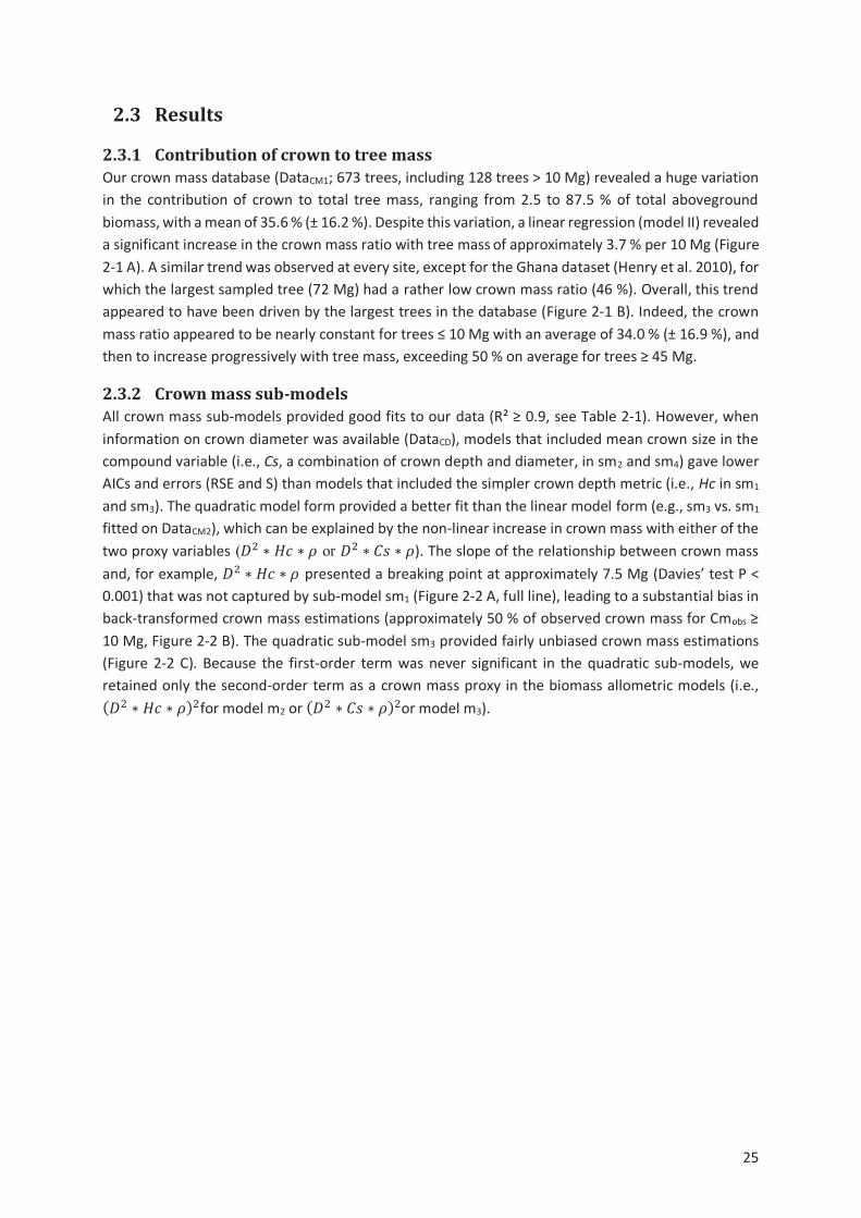
25
2.3 Results
2.3.1 Contribution of crown to tree mass
Our crown mass database (DataCM1; 673 trees, including 128 trees > 10 Mg) revealed a huge variation
in the contribution of crown to total tree mass, ranging from 2.5 to 87.5 % of total aboveground
biomass, with a mean of 35.6 % (± 16.2 %). Despite this variation, a linear regression (model II) revealed
a significant increase in the crown mass ratio with tree mass of approximately 3.7 % per 10 Mg (Figure
2-1 A). A similar trend was observed at every site, except for the Ghana dataset (Henry et al. 2010), for
which the largest sampled tree (72 Mg) had a rather low crown mass ratio (46 %). Overall, this trend
appeared to have been driven by the largest trees in the database (Figure 2-1 B). Indeed, the crown
mass ratio appeared to be nearly constant for trees ≤ 10 Mg with an average of 34.0 % (± 16.9 %), and
then to increase progressively with tree mass, exceeding 50 % on average for trees ≥ 45 Mg.
2.3.2 Crown mass sub-models
All crown mass sub-models provided good fits to our data (R² ≥ 0.9, see Table 2-1). However, when
information on crown diameter was available (DataCD), models that included mean crown size in the
compound variable (i.e., Cs, a combination of crown depth and diameter, in sm2 and sm4) gave lower
AICs and errors (RSE and S) than models that included the simpler crown depth metric (i.e., Hc in sm1
and sm3). The quadratic model form provided a better fit than the linear model form (e.g., sm3 vs. sm1
fitted on DataCM2), which can be explained by the non-linear increase in crown mass with either of the
two proxy variables (!+ " #J " $ or !+ " <> " $). The slope of the relationship between crown mass
and, for example, !+ " #J " $ presented a breaking point at approximately 7.5 Mg (Davies’ test P <
0.001) that was not captured by sub-model sm1 (Figure 2-2 A, full line), leading to a substantial bias in
back-transformed crown mass estimations (approximately 50 % of observed crown mass for Cmobs ≥
10 Mg, Figure 2-2 B). The quadratic sub-model sm3 provided fairly unbiased crown mass estimations
(Figure 2-2 C). Because the first-order term was never significant in the quadratic sub-models, we
retained only the second-order term as a crown mass proxy in the biomass allometric models (i.e.,
*!+ " #J " $,+for model m2 or *!+ " <> " $,+or model m3).
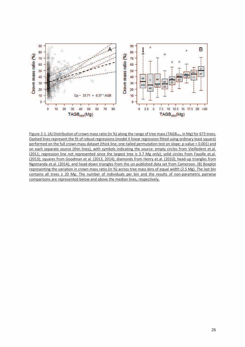
26
Figure 2-1. (A) Distribution of crown mass ratio (in %) along the range of tree mass (TAGBobs, in Mg) for 673 trees. Dashed lines represent the fit of robust regressions (model II linear regression fitted using ordinary least square) performed on the full crown mass dataset (thick line; one-tailed permutation test on slope: p-value < 0.001) and on each separate source (thin lines), with symbols indicating the source: empty circles from Vieilledent et.al. (2011; regression line not represented since the largest tree is 3.7 Mg only); solid circles from Fayolle et.al. (2013); squares from Goodman et al. (2013, 2014); diamonds from Henry et.al. (2010); head-up triangles from Ngomanda et.al. (2014); and head-down triangles from the un-published data set from Cameroon. (B) Boxplot representing the variation in crown mass ratio (in %) across tree mass bins of equal width (2.5 Mg). The last bin contains all trees ≥ 20 Mg. The number of individuals per bin and the results of non-parametric pairwise comparisons are represented below and above the median lines, respectively.
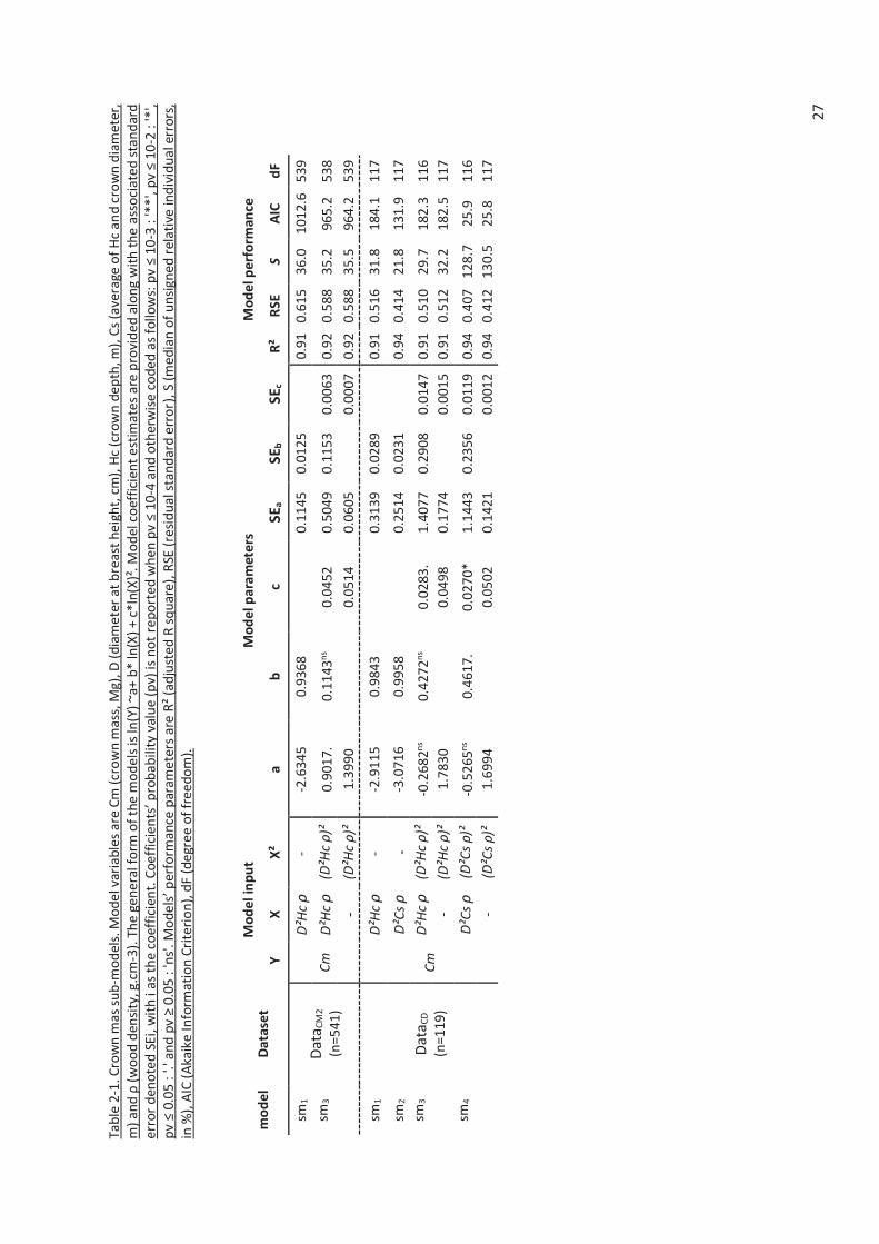
27
Tab
le 2
-1. C
row
n m
as s
ub
-mo
del
s. M
ode
l var
iabl
es a
re C
m (
cro
wn
mas
s, M
g), D
(di
amet
er a
t b
reas
t he
igh
t, c
m),
Hc
(cro
wn
dep
th, m
), C
s (a
vera
ge o
f H
c an
d cr
ow
n d
iam
eter
, m
) an
d ρ
(w
oo
d d
ensi
ty, g
.cm
-3).
Th
e ge
ner
al f
orm
of
the
mo
del
s is
ln(Y
) ~a
+ b*
ln(X
) +
c*ln
(X)²
. Mo
del
co
effi
cien
t es
tim
ates
are
pro
vid
ed a
lon
g w
ith
th
e as
soci
ated
sta
nd
ard
e
rro
r d
en
ote
d S
Ei,
wit
h i
as
the
co
eff
icie
nt.
Co
eff
icie
nts
’ p
rob
ab
ility
val
ue
(p
v) i
s n
ot
rep
ort
ed
wh
en
pv
≤ 1
0-4
an
d o
the
rwis
e c
od
ed
as
foll
ow
s: p
v ≤
10
-3 :
'**
', p
v ≤
10
-2 :
'*',
pv
≤ 0
.05
: '.
' an
d p
v ≥
0.0
5 :
'ns'
. M
od
els
’ p
erf
orm
an
ce p
aram
ete
rs a
re R
² (a
dju
ste
d R
sq
ua
re),
RSE
(re
sid
ua
l sta
nd
ard
err
or)
, S (
med
ian
of
un
sign
ed r
elat
ive
ind
ivid
ual
err
ors,
in
%),
AIC
(A
kaik
e In
form
atio
n C
rite
rio
n),
dF
(deg
ree
of
free
dom
).
mo
de
l D
ata
set
Mo
de
l in
pu
t M
od
el p
ara
me
ters
M
od
el p
erf
orm
an
ce
Y
X
X²
a
b
c S
Ea
SE
b
SE
c R
² R
SE
S
A
IC
dF
sm1
Dat
a CM
2
(n=5
41)
Cm
D²H
c ρ
-
-2
.634
5 0.
9368
0.11
45
0.01
25
0.
91
0.61
5 36
.0
1012
.6
539
sm3
D²H
c ρ
(D
²Hc
ρ)²
0.
9017
. 0.
1143
ns
0.04
52
0.50
49
0.11
53
0.00
63
0.92
0.
588
35.2
96
5.2
538
- (D
²Hc
ρ)²
1.
3990
0.05
14
0.06
05
0.
0007
0.
92
0.58
8 35
.5
964.
2 53
9
sm1
Dat
a CD
(n=1
19)
Cm
D²H
c ρ
-
-2
.911
5 0.
9843
0.31
39
0.02
89
0.
91
0.51
6 31
.8
184.
1 11
7
sm2
D²C
s ρ
-
-3.0
716
0.99
58
0.
2514
0.
0231
0.94
0.
414
21.8
13
1.9
117
sm3
D²H
c ρ
(D
²Hc
ρ)²
-0
.268
2ns
0.42
72n
s 0.
0283
. 1.
4077
0.
2908
0.
0147
0.
91
0.51
0 29
.7
182.
3 11
6
- (D
²Hc
ρ)²
1.
7830
0.04
98
0.17
74
0.
0015
0.
91
0.51
2 32
.2
182.
5 11
7
sm4
D²C
s ρ
(D
²Cs
ρ)²
-0
.526
5ns
0.46
17.
0.02
70*
1.14
43
0.23
56
0.01
19
0.94
0.
407
128.
7 25
.9
116
- (D
²Cs
ρ)²
1.
6994
0.05
02
0.14
21
0.
0012
0.
94
0.41
2 13
0.5
25.8
11
7
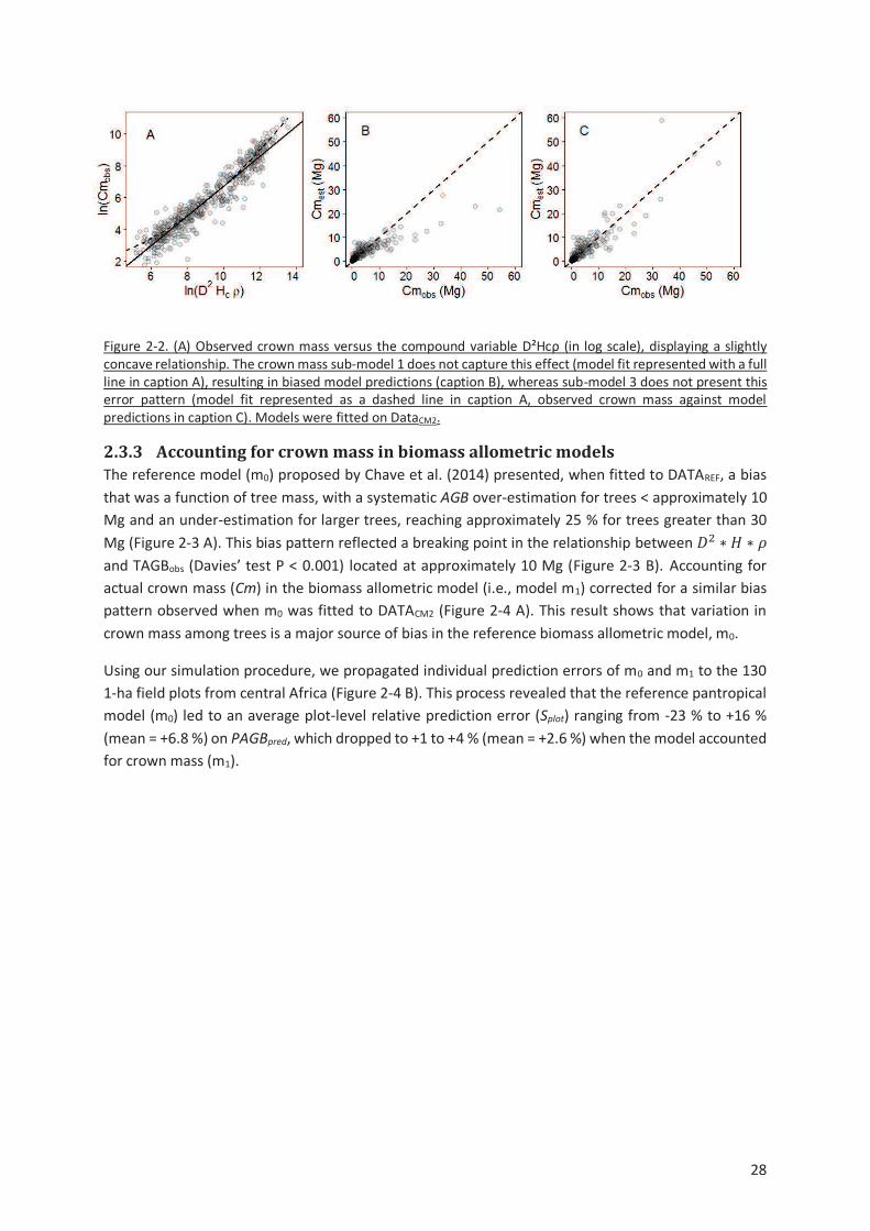
28
Figure 2-2. (A) Observed crown mass versus the compound variable D²Hcρ (in log scale), displaying a slightly concave relationship. The crown mass sub-model 1 does not capture this effect (model fit represented with a full line in caption A), resulting in biased model predictions (caption B), whereas sub-model 3 does not present this error pattern (model fit represented as a dashed line in caption A, observed crown mass against model predictions in caption C). Models were fitted on DataCM2.
2.3.3 Accounting for crown mass in biomass allometric models
The reference model (m0) proposed by Chave et al. (2014) presented, when fitted to DATAREF, a bias
that was a function of tree mass, with a systematic AGB over-estimation for trees < approximately 10
Mg and an under-estimation for larger trees, reaching approximately 25 % for trees greater than 30
Mg (Figure 2-3 A). This bias pattern reflected a breaking point in the relationship between !+ " # " $
and TAGBobs (Davies’ test P < 0.001) located at approximately 10 Mg (Figure 2-3 B). Accounting for
actual crown mass (Cm) in the biomass allometric model (i.e., model m1) corrected for a similar bias
pattern observed when m0 was fitted to DATACM2 (Figure 2-4 A). This result shows that variation in
crown mass among trees is a major source of bias in the reference biomass allometric model, m0.
Using our simulation procedure, we propagated individual prediction errors of m0 and m1 to the 130
1-ha field plots from central Africa (Figure 2-4 B). This process revealed that the reference pantropical
model (m0) led to an average plot-level relative prediction error (Splot) ranging from -23 % to +16 %
(mean = +6.8 %) on PAGBpred, which dropped to +1 to +4 % (mean = +2.6 %) when the model accounted
for crown mass (m1).
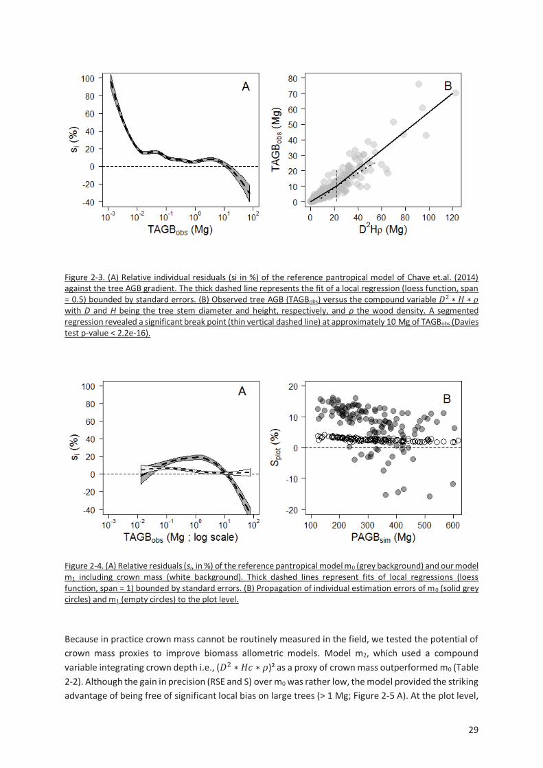
29
Figure 2-3. (A) Relative individual residuals (si in %) of the reference pantropical model of Chave et.al. (2014) against the tree AGB gradient. The thick dashed line represents the fit of a local regression (loess function, span = 0.5) bounded by standard errors. (B) Observed tree AGB (TAGBobs) versus the compound variable !+ " # " $ with D and H being the tree stem diameter and height, respectively, and ρ the wood density. A segmented regression revealed a significant break point (thin vertical dashed line) at approximately 10 Mg of TAGBobs (Davies test p-value < 2.2e-16).
Figure 2-4. (A) Relative residuals (si, in %) of the reference pantropical model m0 (grey background) and our model m1 including crown mass (white background). Thick dashed lines represent fits of local regressions (loess function, span = 1) bounded by standard errors. (B) Propagation of individual estimation errors of m0 (solid grey circles) and m1 (empty circles) to the plot level.
Because in practice crown mass cannot be routinely measured in the field, we tested the potential of
crown mass proxies to improve biomass allometric models. Model m2, which used a compound
variable integrating crown depth i.e., (!+ " #J " $)² as a proxy of crown mass outperformed m0 (Table
2-2). Although the gain in precision (RSE and S) over m0 was rather low, the model provided the striking
advantage of being free of significant local bias on large trees (> 1 Mg; Figure 2-5 A). At the plot level,
6 Cm
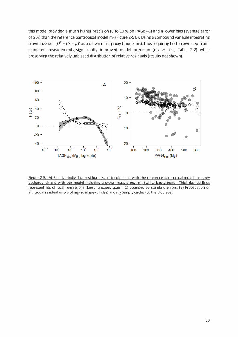
30
this model provided a much higher precision (0 to 10 % on PAGBpred) and a lower bias (average error
of 5 %) than the reference pantropical model m0 (Figure 2-5 B). Using a compound variable integrating
crown size i.e., (!+ " <> " $)² as a crown mass proxy (model m3), thus requiring both crown depth and
diameter measurements,0significantly improved model precision (m3 vs. m2, Table 2-2) while
preserving the relatively unbiased distribution of relative residuals (results not shown).
Figure 2-5. (A) Relative individual residuals (si, in %) obtained with the reference pantropical model m0 (grey background) and with our model including a crown mass proxy, m2 (white background). Thick dashed lines represent fits of local regressions (loess function, span = 1) bounded by standard errors. (B) Propagation of individual residual errors of m0 (solid grey circles) and m2 (empty circles) to the plot level.
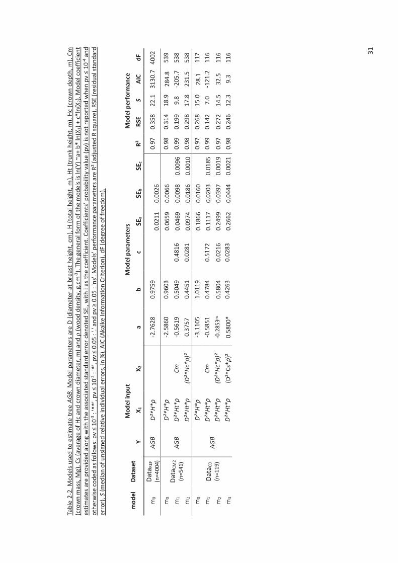
31
Tab
le 2
-2.
Mo
del
s u
sed
to
esti
mat
e tr
ee A
GB
. M
od
el p
aram
eter
s ar
e D
(d
iam
eter
at
brea
st h
eigh
t, c
m),
H (
tota
l hei
ght,
m),
Ht
(tru
nk
hei
ght,
m),
Hc
(cro
wn
dep
th, m
), C
m
(cro
wn
mas
s, M
g), C
s (a
vera
ge o
f H
c an
d c
row
n d
iam
eter
, m)
and
ρ (
wo
od d
ensi
ty, g
.cm
-3).
Th
e ge
ner
al f
orm
of
the
mo
dels
is ln
(Y)
~a+
b*
ln(X
1)
+ c*
ln(X
2). M
od
el c
oeff
icie
nt
esti
mat
es a
re p
rovi
ded
alo
ng w
ith
the
asso
ciat
ed s
tan
dar
d er
ror
den
ote
d SE
i, w
ith
i as
the
coef
fici
ent.
Co
effi
cien
ts’ p
rob
ab
ility
va
lue
(p
v) i
s n
ot
rep
ort
ed
wh
en
pv
≤ 1
0-4
an
d o
ther
wis
e co
ded
as
follo
ws:
pv
≤ 1
0-3
: '*
*', p
v ≤
10
-2 :
'*',
pv
≤ 0
.05
: '.'
an
d p
v ≥
0.0
5 :
'ns'
. Mo
de
ls’
per
form
ance
par
amet
ers
are
R²
(ad
just
ed R
sq
uar
e), R
SE (
resi
du
al s
tan
dar
d er
ror)
, S (
med
ian
of
un
sign
ed r
elat
ive
ind
ivid
ual
err
ors,
in %
), A
IC (
Aka
ike
Info
rmat
ion
Cri
teri
on)
, dF
(deg
ree
of
free
dom
).
mo
de
l D
ata
set
Mo
de
l in
pu
t M
od
el p
ara
me
ters
M
od
el p
erf
orm
an
ce
Y
X1
X2
a
b
c S
Ea
SE
b
SE
c R
² R
SE
S
AIC
d
F
m0
Dat
a REF
(n
=400
4)
AG
B
D²*
H*
ρ
-2
.762
8 0.
9759
0.02
11
0.00
26
0.
97
0.35
8 22
.1
3130
.7
4002
m0
Dat
a CM
2
(n=5
41)
AG
B
D²*
H*
ρ
-2
.586
0 0.
9603
0.06
59
0.00
66
0.
98
0.31
4 18
.9
284.
8 53
9
m1
D²*
Ht*
ρ
Cm
-0
.561
9 0.
5049
0.
4816
0.
0469
0.
0098
0.
0096
0.
99
0.19
9 9.
8 -2
05.7
53
8
m2
D²*
Ht*
ρ
(D²*
Hc*
ρ)²
0.
3757
0.
4451
0.
0281
0.
0974
0.
0186
0.
0010
0.
98
0.29
8 17
.8
231.
5 53
8
m0
Dat
a CD
(n=1
19)
AG
B
D²*
H*
ρ
-3
.110
5 1.
0119
0.18
66
0.01
60
0.
97
0.26
8 15
.0
28.1
11
7
m1
D²*
Ht*
ρ
Cm
-0
.585
1 0.
4784
0.
5172
0.
1117
0.
0203
0.
0185
0.
99
0.14
2 7.
0 -1
21.2
11
6
m2
D²*
Ht*
ρ
(D²*
Hc*
ρ)²
-0
.285
3ns
0.58
04
0.02
16
0.24
99
0.03
97
0.00
19
0.97
0.
272
14.5
32
.5
116
m3
D²*
Ht*
ρ
(D²*
Cs*
ρ)²
0.
5800
* 0.
4263
0.
0283
0.
2662
0.
0444
0.
0021
0.
98
0.24
6 12
.3
9.3
116
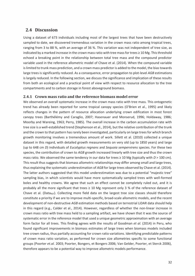
32
2.4 Discussion
Using a dataset of 673 individuals including most of the largest trees that have been destructively
sampled to date, we discovered tremendous variation in the crown mass ratio among tropical trees,
ranging from 3 to 88 %, with an average of 36 %. This variation was not independent of tree size, as
indicated by a marked increase in the crown mass ratio with tree mass for trees ≥ 10 Mg. This threshold
echoed a breaking point in the relationship between total tree mass and the compound predictor
variable used in the reference allometric model of Chave et al. (2014). When the compound variable
is limited to trunk mass prediction, and a crown mass predictor is added to the model, the bias towards
large trees is significantly reduced. As a consequence, error propagation to plot-level AGB estimations
is largely reduced. In the following section, we discuss the significance and implication of these results
from both an ecological and a practical point of view with respect to resource allocation to the tree
compartments and to carbon storage in forest aboveground biomass.
2.4.1 Crown mass ratio and the reference biomass model error
We observed an overall systematic increase in the crown mass ratio with tree mass. This ontogenetic
trend has already been reported for some tropical canopy species (O’Brien et al., 1995) and likely
reflects changes in the pattern of resource allocation underlying crown edification in most forest
canopy trees (Barthélémy and Caraglio, 2007; Hasenauer and Monserud, 1996; Holdaway, 1986;
Moorby and Wareing, 1963; Perry, 1985). The overall increase in the carbon accumulation rate with
tree size is a well-established trend (Stephenson et al., 2014), but the relative contribution of the trunk
and the crown to that pattern has rarely been investigated, particularly on large trees for which branch
growth monitoring involves a tremendous amount of work. Sillett et al. (2010) collected a unique
dataset in this regard, with detailed growth measurements on very old (up to 1850 years) and large
(up to 648 cm D) individuals of Eucalyptus regnans and Sequoia sempervirens species. For these two
species, the contribution of crown to AGB growth increased linearly with tree size and thus the crown
mass ratio. We observed the same tendency in our data for trees ≥ 10 Mg (typically with D > 100 cm).
This result thus suggests that biomass allometric relationships may differ among small and large trees,
thus explaining the systematic underestimation of AGB for large trees observed by Chave et al. (2014).
The latter authors suggested that this model underestimation was due to a potential “majestic tree”
sampling bias, in which scientists would have more systematically sampled trees with well-formed
boles and healthy crowns. We agree that such an effect cannot be completely ruled out, and it is
probably all the more significant that trees ≥ 10 Mg represent only 3 % of the reference dataset of
Chave et al. (DataREF). Collecting more field data on the largest tree size classes should therefore
constitute a priority if we are to improve multi-specific, broad-scale allometric models, and the recent
development of non-destructive AGB estimation methods based on terrestrial LiDAR data should help
in this regard (e.g., Calder et al., 2014). However, regardless of whether the non-linear increase in
crown mass ratio with tree mass held to a sampling artifact, we have shown that it was the source of
systematic error in the reference model that used a unique geometric approximation with an average
form factor for all trees. This finding agrees with the results of Goodman et al. (2014) in Peru, who
found significant improvements in biomass estimates of large trees when biomass models included
tree crown radius, thus partially accounting for crown ratio variations. Identifying predictable patterns
of crown mass ratio variation, as performed for crown size allometries specific to some functional
groups (Poorter et.al. 2003; Poorter, Bongers, et Bongers 2006; Van Gelder, Poorter, et Sterck 2006),
therefore appears to be a potential way to improve allometric models performance.
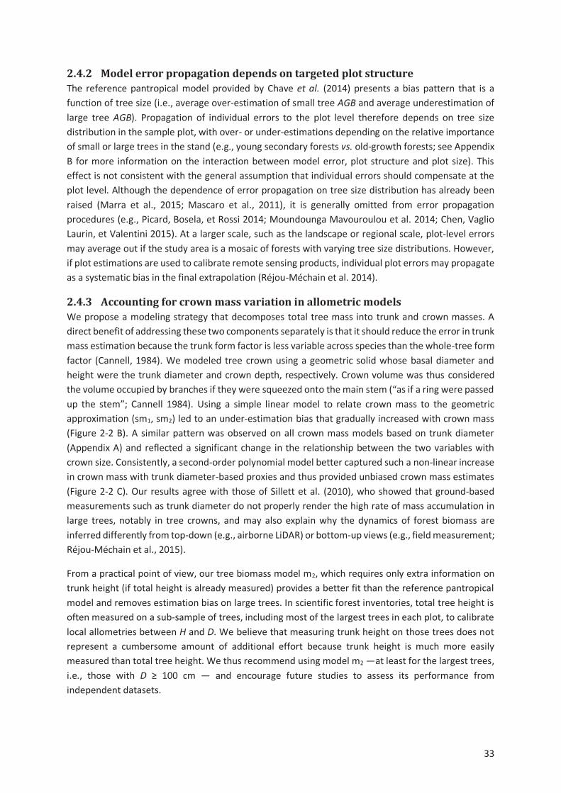
33
2.4.2 Model error propagation depends on targeted plot structure
The reference pantropical model provided by Chave et al. (2014) presents a bias pattern that is a
function of tree size (i.e., average over-estimation of small tree AGB and average underestimation of
large tree AGB). Propagation of individual errors to the plot level therefore depends on tree size
distribution in the sample plot, with over- or under-estimations depending on the relative importance
of small or large trees in the stand (e.g., young secondary forests vs. old-growth forests; see Appendix
B for more information on the interaction between model error, plot structure and plot size). This
effect is not consistent with the general assumption that individual errors should compensate at the
plot level. Although the dependence of error propagation on tree size distribution has already been
raised (Marra et al., 2015; Mascaro et al., 2011), it is generally omitted from error propagation
procedures (e.g., Picard, Bosela, et Rossi 2014; Moundounga Mavouroulou et al. 2014; Chen, Vaglio
Laurin, et Valentini 2015). At a larger scale, such as the landscape or regional scale, plot-level errors
may average out if the study area is a mosaic of forests with varying tree size distributions. However,
if plot estimations are used to calibrate remote sensing products, individual plot errors may propagate
as a systematic bias in the final extrapolation (Réjou-Méchain et al. 2014).
2.4.3 Accounting for crown mass variation in allometric models
We propose a modeling strategy that decomposes total tree mass into trunk and crown masses. A
direct benefit of addressing these two components separately is that it should reduce the error in trunk
mass estimation because the trunk form factor is less variable across species than the whole-tree form
factor (Cannell, 1984). We modeled tree crown using a geometric solid whose basal diameter and
height were the trunk diameter and crown depth, respectively. Crown volume was thus considered
the volume occupied by branches if they were squeezed onto the main stem (“as if a ring were passed
up the stem”; Cannell 1984). Using a simple linear model to relate crown mass to the geometric
approximation (sm1, sm2) led to an under-estimation bias that gradually increased with crown mass
(Figure 2-2 B). A similar pattern was observed on all crown mass models based on trunk diameter
(Appendix A) and reflected a significant change in the relationship between the two variables with
crown size. Consistently, a second-order polynomial model better captured such a non-linear increase
in crown mass with trunk diameter-based proxies and thus provided unbiased crown mass estimates
(Figure 2-2 C). Our results agree with those of Sillett et al. (2010), who showed that ground-based
measurements such as trunk diameter do not properly render the high rate of mass accumulation in
large trees, notably in tree crowns, and may also explain why the dynamics of forest biomass are
inferred differently from top-down (e.g., airborne LiDAR) or bottom-up views (e.g., field measurement;
Réjou-Méchain et al., 2015).
From a practical point of view, our tree biomass model m2, which requires only extra information on
trunk height (if total height is already measured) provides a better fit than the reference pantropical
model and removes estimation bias on large trees. In scientific forest inventories, total tree height is
often measured on a sub-sample of trees, including most of the largest trees in each plot, to calibrate
local allometries between H and D. We believe that measuring trunk height on those trees does not
represent a cumbersome amount of additional effort because trunk height is much more easily
measured than total tree height. We thus recommend using model m2 —at least for the largest trees,
i.e., those with D ≥ 100 cm — and encourage future studies to assess its performance from
independent datasets.
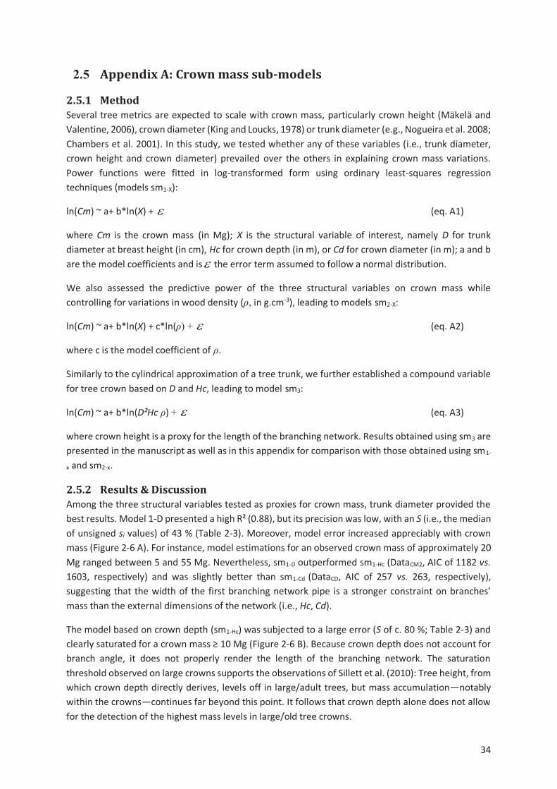
34
2.5 Appendix A: Crown mass sub-models
2.5.1 Method
Several tree metrics are expected to scale with crown mass, particularly crown height (Mäkelä and
Valentine, 2006), crown diameter (King and Loucks, 1978) or trunk diameter (e.g., Nogueira et al. 2008;
Chambers et al. 2001). In this study, we tested whether any of these variables (i.e., trunk diameter,
crown height and crown diameter) prevailed over the others in explaining crown mass variations.
Power functions were fitted in log-transformed form using ordinary least-squares regression
techniques (models sm1-X):
ln(Cm) ~ a+ b*ln(X) + e (eq. A1)
where Cm is the crown mass (in Mg); X is the structural variable of interest, namely D for trunk
diameter at breast height (in cm), Hc for crown depth (in m), or Cd for crown diameter (in m); a and b
are the model coefficients and ise the error term assumed to follow a normal distribution.
We also assessed the predictive power of the three structural variables on crown mass while
controlling for variations in wood density (ρ, in g.cm-3), leading to models sm2-X:
ln(Cm) ~ a+ b*ln(X) + c*ln(ρ) + e (eq. A2)
where c is the model coefficient of ρ.
Similarly to the cylindrical approximation of a tree trunk, we further established a compound variable
for tree crown based on D and Hc, leading to model sm3:
ln(Cm) ~ a+ b*ln(D²Hc ρ) + e (eq. A3)
where crown height is a proxy for the length of the branching network. Results obtained using sm3 are
presented in the manuscript as well as in this appendix for comparison with those obtained using sm1-
x and sm2-x.
2.5.2 Results & Discussion
Among the three structural variables tested as proxies for crown mass, trunk diameter provided the
best results. Model 1-D presented a high R² (0.88), but its precision was low, with an S (i.e., the median
of unsigned si values) of 43 % (Table 2-3). Moreover, model error increased appreciably with crown
mass (Figure 2-6 A). For instance, model estimations for an observed crown mass of approximately 20
Mg ranged between 5 and 55 Mg. Nevertheless, sm1-D outperformed sm1-Hc (DataCM2, AIC of 1182 vs.
1603, respectively) and was slightly better than sm1-Cd (DataCD, AIC of 257 vs. 263, respectively),
suggesting that the width of the first branching network pipe is a stronger constraint on branches'
mass than the external dimensions of the network (i.e., Hc, Cd).
The model based on crown depth (sm1-Hc) was subjected to a large error (S of c. 80 %; Table 2-3) and
clearly saturated for a crown mass ≥ 10 Mg (Figure 2-6 B). Because crown depth does not account for
branch angle, it does not properly render the length of the branching network. The saturation
threshold observed on large crowns supports the observations of Sillett et al. (2010): Tree height, from
which crown depth directly derives, levels off in large/adult trees, but mass accumulation—notably
within the crowns—continues far beyond this point. It follows that crown depth alone does not allow
for the detection of the highest mass levels in large/old tree crowns.
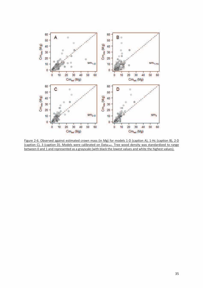
35
Figure 2-6. Observed against estimated crown mass (in Mg) for models 1-D (caption A), 1-Hc (caption B), 2-D (caption C), 3 (caption D). Models were calibrated on DataCM2. Tree wood density was standardized to range between 0 and 1 and represented as a grayscale (with black the lowest values and white the highest values).
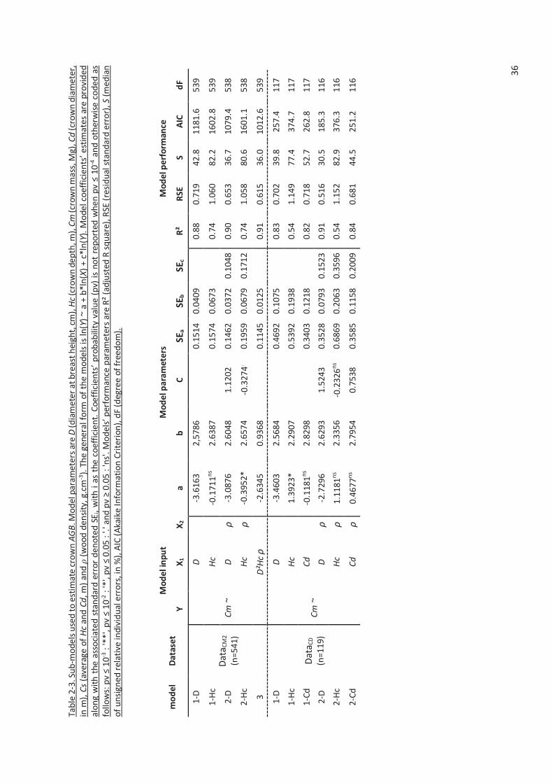
36
Tab
le 2
-3. S
ub
-mo
dels
use
d to
est
imat
e cr
ow
n A
GB
. Mo
del
par
amet
ers
are
D (d
iam
eter
at
brea
st h
eigh
t, c
m),
Hc
(cro
wn
dep
th, m
), C
m (c
row
n m
ass,
Mg)
, Cd
(cro
wn
diam
eter
, in
m),
Cs
(ave
rage
of
Hc
and
Cd
, m)
and ρ
(w
ood
den
sity
, g.c
m-3
). T
he
gene
ral f
orm
of
the
mo
dels
is ln
(Y)
~ a
+ b
*ln
(X)
+ c*
ln(Y
). M
ode
l co
effi
cien
ts’ e
stim
ates
are
pro
vid
ed
alo
ng
wit
h t
he a
sso
ciat
ed s
tan
dar
d er
ror
den
ote
d SE
i, w
ith
i as
the
co
effi
cien
t. C
oeff
icie
nts
’ p
rob
ab
ility
val
ue
(p
v) i
s n
ot
rep
ort
ed
wh
en
pv
≤ 1
0-4
an
d o
ther
wis
e co
ded
as
follo
ws:
pv
≤ 1
0-3
: '*
*', p
v ≤
10
-2 :
'*',
pv
≤ 0
.05
: '.'
an
d p
v ≥
0.0
5 :
'ns'
. Mo
de
ls’
pe
rfo
rma
nce
par
ame
ters
are
R²
(ad
just
ed
R s
qu
are
), R
SE (
resi
du
al s
tan
dar
d e
rro
r), S
(m
edia
n
of
un
sign
ed r
elat
ive
indi
vid
ual
err
ors
, in
%),
AIC
(A
kaik
e In
form
atio
n C
rite
rion
), d
F (d
egre
e of
fre
edo
m).
mo
de
l D
ata
set
Mo
de
l in
pu
t M
od
el p
ara
me
ters
M
od
el p
erf
orm
an
ce
Y
X1
X2
a
b
C
SE
a
SE
b
SE
c R
² R
SE
S
AIC
d
F
1-D
Dat
a CM
2
(n=5
41)
Cm
~
D
-3
.616
3 2,
5786
0.15
14
0.04
09
0.
88
0.71
9 42
.8
1181
.6
539
1-H
c H
c
-0.1
711n
s 2.
6387
0.15
74
0.06
73
0.
74
1.06
0 82
.2
1602
.8
539
2-D
D
ρ
-3
.087
6 2.
6048
1.
1202
0.
1462
0.
0372
0.
1048
0.
90
0.65
3 36
.7
1079
.4
538
2-H
c H
c ρ
-0
.395
2*
2.65
74
-0.3
274.
0.19
59
0.06
79
0.17
12
0.74
1.
058
80.6
16
01.1
53
8
3 D
²Hc
ρ
-2
.634
5 0.
9368
0.11
45
0.01
25
0.
91
0.61
5 36
.0
1012
.6
539
1-D
Dat
a CD
(n=1
19)
Cm
~
D
-3
.460
3 2.
5684
0.46
92
0.10
75
0.
83
0.70
2 39
.8
257.
4 11
7
1-H
c H
c
1.39
23*
2.29
07
0.
5392
0.
1938
0.54
1.
149
77.4
37
4.7
117
1-C
d
Cd
-0.1
181n
s 2.
8298
0.34
03
0.12
18
0.
82
0.71
8 52
.7
262.
8 11
7
2-D
D
ρ
-2
.729
6 2.
6293
1.
5243
0.
3528
0.
0793
0.
1523
0.
91
0.51
6 30
.5
185.
3 11
6
2-H
c H
c ρ
1.
1181
ns
2.33
56
-0.2
326n
s 0.
6869
0.
2063
0.
3596
0.
54
1.15
2 82
.9
376.
3 11
6
2-C
d
Cd
ρ
0.
4677
ns
2.79
54
0.75
38
0.35
85
0.11
58
0.20
09
0.84
0.
681
44.5
25
1.2
116
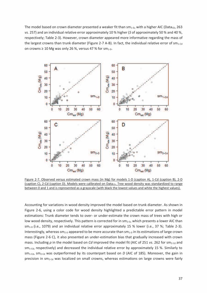
37
The model based on crown diameter presented a weaker fit than sm1-D, with a higher AIC (DataCD, 263
vs. 257) and an individual relative error approximately 10 % higher (S of approximately 50 % and 40 %,
respectively; Table 2-3). However, crown diameter appeared more informative regarding the mass of
the largest crowns than trunk diameter (Figure 2-7 A-B). In fact, the individual relative error of sm1-Cd
on crowns ≥ 10 Mg was only 26 %, versus 47 % for sm1-D.
Figure 2-7. Observed versus estimated crown mass (in Mg) for models 1-D (caption A), 1-Cd (caption B), 2-D (caption C), 2-Cd (caption D). Models were calibrated on DataCD. Tree wood density was standardized to range between 0 and 1 and is represented as a grayscale (with black the lowest values and white the highest values).
Accounting for variations in wood density improved the model based on trunk diameter. As shown in
Figure 2-6, using a color code for wood density highlighted a predictable error pattern in model
estimations: Trunk diameter tends to over- or under-estimate the crown mass of trees with high or
low wood density, respectively. This pattern is corrected for in sm2-D, which presents a lower AIC than
sm1-D (i.e., 1079) and an individual relative error approximately 15 % lower (i.e., 37 %; Table 2-3).
Interestingly, whereas sm2-D appeared to be more accurate than sm1-D in its estimations of large crown
mass (Figure 2-6 C), it also presented an under-estimation bias that gradually increased with crown
mass. Including ρ in the model based on Cd improved the model fit (AIC of 251 vs. 262 for sm2-Cd and
sm1-Cd, respectively) and decreased the individual relative error by approximately 15 %. Similarly to
sm1-Cd, sm2-Cd was outperformed by its counterpart based on D (AIC of 185). Moreover, the gain in
precision in sm2-Cd was localized on small crowns, whereas estimations on large crowns were fairly
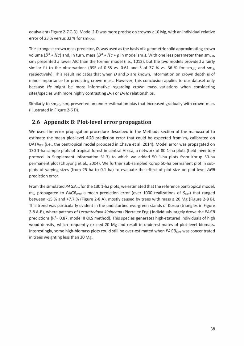
38
equivalent (Figure 2-7 C-D). Model 2-D was more precise on crowns ≥ 10 Mg, with an individual relative
error of 23 % versus 32 % for sm2-Cd.
The strongest crown mass predictor, D, was used as the basis of a geometric solid approximating crown
volume (!² " #J) and, in turn, mass (!² " #J " . in model sm3). With one less parameter than sm2-D,
sm3 presented a lower AIC than the former model (i.e., 1012), but the two models provided a fairly
similar fit to the observations (RSE of 0.65 vs. 0.61 and S of 37 % vs. 36 % for sm2-D and sm3,
respectively). This result indicates that when D and ρ are known, information on crown depth is of
minor importance for predicting crown mass. However, this conclusion applies to our dataset only
because Hc might be more informative regarding crown mass variations when considering
sites/species with more highly contrasting D-H or D-Hc relationships.
Similarly to sm2-D, sm3 presented an under-estimation bias that increased gradually with crown mass
(illustrated in Figure 2-6 D).
2.6 Appendix B: Plot-level error propagation
We used the error propagation procedure described in the Methods section of the manuscript to
estimate the mean plot-level AGB prediction error that could be expected from m0 calibrated on
DATAREF (i.e., the pantropical model proposed in Chave et al. 2014). Model error was propagated on
130 1-ha sample plots of tropical forest in central Africa, a network of 80 1-ha plots (field inventory
protocol in Supplement Information S1.3) to which we added 50 1-ha plots from Korup 50-ha
permanent plot (Chuyong et al., 2004). We further sub-sampled Korup 50-ha permanent plot in sub-
plots of varying sizes (from 25 ha to 0.1 ha) to evaluate the effect of plot size on plot-level AGB
prediction error.
From the simulated PAGBsim for the 130 1-ha plots, we estimated that the reference pantropical model,
m0, propagated to PAGBpred a mean prediction error (over 1000 realizations of Splot) that ranged
between -15 % and +7.7 % (Figure 2-8 A), mostly caused by trees with mass ≥ 20 Mg (Figure 2-8 B).
This trend was particularly evident in the undisturbed evergreen stands of Korup (triangles in Figure
2-8 A-B), where patches of Lecomtedoxa klaineana (Pierre ex Engl) individuals largely drove the PAGB
predictions (R²= 0.87, model II OLS method). This species generates high-statured individuals of high
wood density, which frequently exceed 20 Mg and result in underestimates of plot-level biomass.
Interestingly, some high-biomass plots could still be over-estimated when PAGBpred was concentrated
in trees weighting less than 20 Mg.
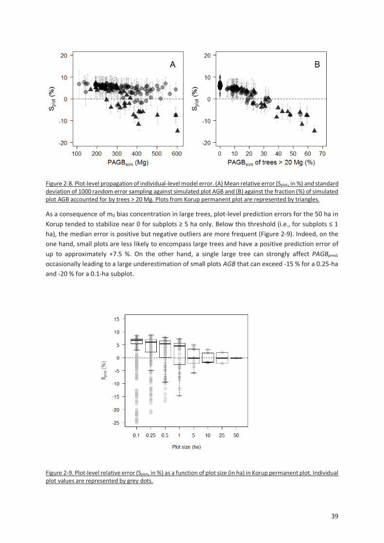
39
Figure 2-8. Plot-level propagation of individual-level model error. (A) Mean relative error (Splot, in %) and standard deviation of 1000 random error sampling against simulated plot AGB and (B) against the fraction (%) of simulated plot AGB accounted for by trees > 20 Mg. Plots from Korup permanent plot are represented by triangles.
As a consequence of m0 bias concentration in large trees, plot-level prediction errors for the 50 ha in
Korup tended to stabilize near 0 for subplots ≥ 5 ha only. Below this threshold (i.e., for subplots ≤ 1
ha), the median error is positive but negative outliers are more frequent (Figure 2-9). Indeed, on the
one hand, small plots are less likely to encompass large trees and have a positive prediction error of
up to approximately +7.5 %. On the other hand, a single large tree can strongly affect PAGBpred,
occasionally leading to a large underestimation of small plots AGB that can exceed -15 % for a 0.25-ha
and -20 % for a 0.1-ha subplot.
Figure 2-9. Plot-level relative error (Splot, in %) as a function of plot size (in ha) in Korup permanent plot. Individual plot values are represented by grey dots.

40
Author contributions. Conceived and designed the experiments: PP, NB and RP. Collected data
(unpublished destructive data and field inventories): SM, BS, NGK, ML, DZ, NT, FBB, JKM, GD, VD.
Shared data: GC, DK, DT, AF, AN, MH, RCG. Analyzed the data: PP. Analysis feedback: RP, NB, VR, MRM,
UB. Wrote the paper: PP, RP and MRM. Writing feedback: NB, AF, VR, PC, MH, RCG.
Acknowledgments. Destructive data from Cameroon were collected with the financial support from
the IRD project PPR FTH-AC ‘Changements globaux, biodiversité et santé en zone forestière d’Afrique
Centrale’ and the support and involvement of Alpicam Company. A portion of the plot data were
collected with the support of the CoForTips project as part of the ERA-Net BiodivERsA 2011-2012
European joint call (ANR-12-EBID-0002). PP was supported by an Erasmus Mundus PhD grant from the
2013-2016 Forest, Nature and Society (FONASO) doctoral program.
Data Accessibility.
Destructive sampling data set available at http://dx.doi.org/10.5061/dryad.f2b52.
41
2.7 References
Avitabile, V., Herold, M., Henry, M. and Schmullius, C.: Mapping biomass with remote sensing: a
comparison of methods for the case study of Uganda, Carbon Balance Manag., 6(7), 1–14, 2011.
Baccini, A., Goetz, S. J., Walker, W. S., Laporte, N. T., Sun, M., Sulla-Menashe, D., Hackler, J., Beck, P. S.
A., Dubayah, R. and Friedl, M. A.: Estimated carbon dioxide emissions from tropical deforestation
improved by carbon-density maps, Nat. Clim. Change, 2(3), 182–185, 2012.
Barthélémy, D. and Caraglio, Y.: Plant Architecture: A Dynamic, Multilevel and Comprehensive
Approach to Plant Form, Structure and Ontogeny, Ann. Bot., 99(3), 375–407, doi:10.1093/aob/mcl260,
2007.
Baskerville, G. L.: Use of Logarithmic Regression in the Estimation of Plant Biomass, Can. J. For. Res.,
2(1), 49–53, doi:10.1139/x72-009, 1972.
Bastin, J.-F., Barbier, N., Réjou-Méchain, M., Fayolle, A., Gourlet-Fleury, S., Maniatis, D., de Haulleville,
T., Baya, F., Beeckman, H. and Beina, D.: Seeing Central African forests through their largest trees, Sci.
Rep., 5, 2015.
Beygelzimer, A., Kakadet, S., Langford, J., Arya, S., Mount, D. and Li, S.: FNN: fast nearest neighbor
search algorithms and applications. R package version 1.1., 2013.
Brown, S., Gillespie, A. J. and Lugo, A. E.: Biomass estimation methods for tropical forests with
applications to forest inventory data, For. Sci., 35(4), 881–902, 1989.
Cannell, M. G. R.: Woody biomass of forest stands, For. Ecol. Manag., 8(3–4), 299–312,
doi:10.1016/0378-1127(84)90062-8, 1984.
Chambers, J. Q., dos Santos, J., Ribeiro, R. J. and Higuchi, N.: Tree damage, allometric relationships,
and above-ground net primary production in central Amazon forest, For. Ecol. Manag., 152(1), 73–84,
2001.
Chave, J., Andalo, C., Brown, S., Cairns, M. A., Chambers, J. Q., Eamus, D., Fölster, H., Fromard, F.,
Higuchi, N., Kira, T., Lescure, J.-P., Nelson, B. W., Ogawa, H., Puig, H., Riéra, B. and Yamakura, T.: Tree
allometry and improved estimation of carbon stocks and balance in tropical forests, Oecologia, 145(1),
87–99, doi:10.1007/s00442-005-0100-x, 2005.
Chave, J., Coomes, D., Jansen, S., Lewis, S. L., Swenson, N. G. and Zanne, A. E.: Towards a worldwide
wood economics spectrum, Ecol. Lett., 12(4), 351–366, doi:10.1111/j.1461-0248.2009.01285.x, 2009.
Chave, J., Réjou-Méchain, M., Búrquez, A., Chidumayo, E., Colgan, M. S., Delitti, W. B. C., Duque, A.,
Eid, T., Fearnside, P. M., Goodman, R. C., Henry, M., Martínez-Yrízar, A., Mugasha, W. A., Muller-
Landau, H. C., Mencuccini, M., Nelson, B. W., Ngomanda, A., Nogueira, E. M., Ortiz-Malavassi, E.,
Pélissier, R., Ploton, P., Ryan, C. M., Saldarriaga, J. G. and Vieilledent, G.: Improved allometric models
to estimate the aboveground biomass of tropical trees, Glob. Change Biol., 20(10), 3177–3190,
doi:10.1111/gcb.12629, 2014.
42
Chen, Q., Vaglio Laurin, G. and Valentini, R.: Uncertainty of remotely sensed aboveground biomass
over an African tropical forest: Propagating errors from trees to plots to pixels, Remote Sens. Environ.,
160, 134–143, doi:10.1016/j.rse.2015.01.009, 2015.
Chuyong, G. B., Condit, R., Kenfack, D., Losos, E. C., Moses, S. N., Songwe, N. C. and Thomas, D. W.:
Korup forest dynamics plot, Cameroon, Trop. For. Divers. Dynamism, 506–516, 2004.
Clark, D. B. and Clark, D. A.: Abundance, growth and mortality of very large trees in neotropical lowland
rain forest, For. Ecol. Manag., 80(1–3), 235–244, doi:10.1016/0378-1127(95)03607-5, 1996.
Clark, D. B. and Kellner, J. R.: Tropical forest biomass estimation and the fallacy of misplaced
concreteness, J. Veg. Sci., 23(6), 1191–1196, doi:10.1111/j.1654-1103.2012.01471.x, 2012.
Cleveland, W. S., Grosse, E. and Shyu, W. M.: Local regression models, Stat. Models S, 309–376, 1992.
Eggleston, H. S., Buendia, L., Miwa, K., Ngara, T. and Tanabe, K.: IPCC guidelines for national
greenhouse gas inventories, Inst. Glob. Environ. Strateg. Hayama Jpn., 2006.
Eloy, C.: Leonardo’s rule, self-similarity and wind-induced stresses in trees, Phys. Rev. Lett., 107(25),
doi:10.1103/PhysRevLett.107.258101, 2011.
Enquist, B. J.: Universal scaling in tree and vascular plant allometry: toward a general quantitative
theory linking plant form and function from cells to ecosystems, Tree Physiol., 22(15-16), 1045–1064,
doi:10.1093/treephys/22.15-16.1045, 2002.
Fayolle, A., Doucet, J.-L., Gillet, J.-F., Bourland, N. and Lejeune, P.: Tree allometry in Central Africa:
Testing the validity of pantropical multi-species allometric equations for estimating biomass and
carbon stocks, For. Ecol. Manag., 305, 29–37, doi:10.1016/j.foreco.2013.05.036, 2013.
Freedman, B., Duinker, P. N., Barclay, H., Morash, R. and Prager, U.: Forest biomass and nutrient
studies in central Nova Scotia., Inf. Rep. Marit. For. Res. Cent. Can., (M-X-134), 126 pp., 1982.
Goodman, R. C., Phillips, O. L. and Baker, T. R.: Data from: The importance of crown dimensions to
improve tropical tree biomass estimates, [online] Available from:
http://dx.doi.org/10.5061/dryad.p281 g (Accessed 17 May 2015), 2013.
Goodman, R. C., Phillips, O. L. and Baker, T. R.: The importance of crown dimensions to improve tropical
tree biomass estimates, Ecol. Appl., 24(4), 680–698, 2014.
Hansen, M. C., Potapov, P. V., Moore, R., Hancher, M., Turubanova, S. A., Tyukavina, A., Thau, D.,
Stehman, S. V., Goetz, S. J. and Loveland, T. R.: High-resolution global maps of 21st-century forest cover
change, science, 342(6160), 850–853, 2013.
Harris, N. L., Brown, S., Hagen, S. C., Saatchi, S. S., Petrova, S., Salas, W., Hansen, M. C., Potapov, P. V.
and Lotsch, A.: Baseline map of carbon emissions from deforestation in tropical regions, Science,
336(6088), 1573–1576, 2012.
Hasenauer, H. and Monserud, R. A.: A crown ratio model for Austrian forests, For. Ecol. Manag., 84(1–
3), 49–60, doi:10.1016/0378-1127(96)03768-1, 1996.
43
Henry, M., Besnard, A., Asante, W. A., Eshun, J., Adu-Bredu, S., Valentini, R., Bernoux, M. and Saint-
André, L.: Wood density, phytomass variations within and among trees, and allometric equations in a
tropical rainforest of Africa, For. Ecol. Manag., 260(8), 1375–1388, doi:10.1016/j.foreco.2010.07.040,
2010.
Holdaway, M. R.: Modeling Tree Crown Ratio, For. Chron., 62(5), 451–455, doi:10.5558/tfc62451-5,
1986.
Jenkins, J. C., Chojnacky, D. C., Heath, L. S. and Birdsey, R. A.: National-Scale Biomass Estimators for
United States Tree Species, For. Sci., 49(1), 12–35, 2003.
King, D. and Loucks, O. L.: The theory of tree bole and branch form, Radiat. Environ. Biophys., 15(2),
141–165, doi:10.1007/BF01323263, 1978.
Legendre, P.: lmodel2: Model II Regression. R package version 1.7-0, See Httpcran R-Proj.
Orgwebpackageslmodel2, 2011.
Mäkelä, A. and Harry T.: Crown ratio influences allometric scaling of trees, Ecology, 87(12), 2967–2972,
doi:10.1890/0012-9658(2006)87[2967:CRIASI]2.0.CO;2, 2006.
Malhi, Y., Wood, D., Baker, T. R., Wright, J., Phillips, O. L., Cochrane, T., Meir, P., Chave, J., Almeida, S.
and Arroyo, L.: The regional variation of aboveground live biomass in old�growth Amazonian forests,
Glob. Change Biol., 12(7), 1107–1138, 2006.
Marra, D. M., Higuchi, N., Trumbore, S. E., Ribeiro, G., Santos, J. dos, Carneiro, V. M. C., Lima, A. J. N.,
Chambers, J. Q., Negrón-Juárez, R. I. and Holzwarth, F.: Predicting biomass of hyperdiverse and
structurally complex Central Amazon forests–a virtual approach using extensive field data,
Biogeosciences Discuss., 12, 15537–15581, 2015.
Mascaro, J., Litton, C. M., Hughes, R. F., Uowolo, A. and Schnitzer, S. A.: Minimizing Bias in Biomass
Allometry: Model Selection and Log-Transformation of Data, Biotropica, 43(6), 649–653,
doi:10.1111/j.1744-7429.2011.00798.x, 2011.
McMahon, T. A. and Kronauer, R. E.: Tree structures: deducing the principle of mechanical design, J.
Theor. Biol., 59(2), 443–466, 1976.
Mitchard, E. T., Saatchi, S. S., Baccini, A., Asner, G. P., Goetz, S. J., Harris, N. L. and Brown, S.:
Uncertainty in the spatial distribution of tropical forest biomass: a comparison of pan-tropical maps,
Carbon Balance Manag., 8(1), 10, doi:10.1186/1750-0680-8-10, 2013.
Moorby, J. and Wareing, P. F.: Ageing in Woody Plants, Ann. Bot., 27(2), 291–308, 1963.
Moundounga Mavouroulou, Q., Ngomanda, A., Engone Obiang, N. L., Lebamba, J., Gomat, H., Mankou,
G. S., Loumeto, J., Midoko Iponga, D., Kossi Ditsouga, F., Zinga Koumba, R., Botsika Bobé, K. H.,
Lépengué, N., Mbatchi, B. and Picard, N.: How to improve allometric equations to estimate forest
biomass stocks? Some hints from a central African forest, Can. J. For. Res., 44(7), 685–691,
doi:10.1139/cjfr-2013-0520, 2014.
Muggeo, V. M. R.: Estimating regression models with unknown break-points, Stat. Med., 22(19), 3055–
3071, doi:10.1002/sim.1545, 2003.
44
Ngomanda, A., Engone Obiang, N. L., Lebamba, J., Moundounga Mavouroulou, Q., Gomat, H., Mankou,
G. S., Loumeto, J., Midoko Iponga, D., Kossi Ditsouga, F., Zinga Koumba, R., Botsika Bobé, K. H., Mikala
Okouyi, C., Nyangadouma, R., Lépengué, N., Mbatchi, B. and Picard, N.: Site-specific versus pantropical
allometric equations: Which option to estimate the biomass of a moist central African forest?, For.
Ecol. Manag., 312, 1–9, doi:10.1016/j.foreco.2013.10.029, 2014.
Niklas, K. J.: Size-dependent Allometry of Tree Height, Diameter and Trunk-taper, Ann. Bot., 75(3), 217–
227, doi:10.1006/anbo.1995.1015, 1995.
Nogueira, E. M., Fearnside, P. M., Nelson, B. W., Barbosa, R. I. and Keizer, E. W. H.: Estimates of forest
biomass in the Brazilian Amazon: New allometric equations and adjustments to biomass from wood-
volume inventories, For. Ecol. Manag., 256(11), 1853–1867, 2008.
Pelletier, J., Ramankutty, N. and Potvin, C.: Diagnosing the uncertainty and detectability of emission
reductions for REDD + under current capabilities: an example for Panama, Environ. Res. Lett., 6(2),
024005, doi:10.1088/1748-9326/6/2/024005, 2011.
Perry, D. A.: The competition process in forest stands, Attrib. Trees Crop Plants, 481–506, 1985.
Picard, N., Bosela, F. B. and Rossi, V.: Reducing the error in biomass estimates strongly depends on
model selection, Ann. For. Sci., 1–13, doi:10.1007/s13595-014-0434-9, 2014.
Poorter, L., Bongers, F., Sterck, F. J. and Wöll, H.: Architecture of 53 rain forest tree species differing in
adult stature and shade tolerance, Ecology, 84(3), 602–608, doi:10.1890/0012-
9658(2003)084[0602:AORFTS]2.0.CO;2, 2003.
Poorter, L., Bongers, L. and Bongers, F.: Architecture of 54 moist-forest tree species: traits, trade-offs,
and functional groups, Ecology, 87(5), 1289–1301, doi:10.1890/0012-
9658(2006)87[1289:AOMTST]2.0.CO;2, 2006.
Réjou-Méchain, M., Muller-Landau, H. C., Detto, M., Thomas, S. C., Le Toan, T., Saatchi, S. S., Barreto-
Silva, J. S., Bourg, N. A., Bunyavejchewin, S., Butt, N., Brockelman, W. Y., Cao, M., Cárdenas, D., Chiang,
J.-M., Chuyong, G. B., Clay, K., Condit, R., Dattaraja, H. S., Davies, S. J., Duque, A., Esufali, S., Ewango,
C., Fernando, R. H. S., Fletcher, C. D., Gunatilleke, I. A. U. N., Hao, Z., Harms, K. E., Hart, T. B., Hérault,
B., Howe, R. W., Hubbell, S. P., Johnson, D. J., Kenfack, D., Larson, A. J., Lin, L., Lin, Y., Lutz, J. A., Makana,
J.-R., Malhi, Y., Marthews, T. R., McEwan, R. W., McMahon, S. M., McShea, W. J., Muscarella, R.,
Nathalang, A., Noor, N. S. M., Nytch, C. J., Oliveira, A. A., Phillips, R. P., Pongpattananurak, N., Punchi-
Manage, R., Salim, R., Schurman, J., Sukumar, R., Suresh, H. S., Suwanvecho, U., Thomas, D. W.,
Thompson, J., Uríarte, M., Valencia, R., Vicentini, A., Wolf, A. T., Yap, S., Yuan, Z., Zartman, C. E.,
Zimmerman, J. K. and Chave, J.: Local spatial structure of forest biomass and its consequences for
remote sensing of carbon stocks, Biogeosciences, 11(23), 6827–6840, doi:10.5194/bg-11-6827-2014,
2014.
Réjou-Méchain, M., Tymen, B., Blanc, L., Fauset, S., Feldpausch, T. R., Monteagudo, A., Phillips, O. L.,
Richard, H. and Chave, J.: Using repeated small-footprint LiDAR acquisitions to infer spatial and
temporal variations of a high-biomass Neotropical forest, Remote Sens. Environ., 169, 93–101, 2015.
45
Saatchi, S. S., Harris, N. L., Brown, S., Lefsky, M., Mitchard, E. T., Salas, W., Zutta, B. R., Buermann, W.,
Lewis, S. L. and Hagen, S.: Benchmark map of forest carbon stocks in tropical regions across three
continents, Proc. Natl. Acad. Sci., 108(24), 9899–9904, 2011.
Scrucca, L.: Model-based SIR for dimension reduction, Comput. Stat. Data Anal., 55(11), 3010–3026,
2011.
Shinozaki, K., Yoda, K., Hozumi, K. and Kira, T.: A quantitative analysis of plant form-the pipe model
theory: I. Basic analyses, , 14(3), 97–105, 1964.
Sillett, S. C., Van Pelt, R., Koch, G. W., Ambrose, A. R., Carroll, A. L., Antoine, M. E. and Mifsud, B. M.:
Increasing wood production through old age in tall trees, For. Ecol. Manag., 259(5), 976–994,
doi:10.1016/j.foreco.2009.12.003, 2010.
Sist, P., Mazzei, L., Blanc, L. and Rutishauser, E.: Large trees as key elements of carbon storage and
dynamics after selective logging in the Eastern Amazon, For. Ecol. Manag., 318, 103–109,
doi:10.1016/j.foreco.2014.01.005, 2014.
Slik, J. W., Paoli, G., McGuire, K., Amaral, I., Barroso, J., Bastian, M., Blanc, L., Bongers, F., Boundja, P.
and Clark, C.: Large trees drive forest aboveground biomass variation in moist lowland forests across
the tropics, Glob. Ecol. Biogeogr., 22(12), 1261–1271, 2013.
Stephenson, N. L., Das, A. J., Condit, R., Russo, S. E., Baker, P. J., Beckman, N. G., Coomes, D. A., Lines,
E. R., Morris, W. K., Rüger, N., Álvarez, E., Blundo, C., Bunyavejchewin, S., Chuyong, G., Davies, S. J.,
Duque, Á., Ewango, C. N., Flores, O., Franklin, J. F., Grau, H. R., Hao, Z., Harmon, M. E., Hubbell, S. P.,
Kenfack, D., Lin, Y., Makana, J.-R., Malizia, A., Malizia, L. R., Pabst, R. J., Pongpattananurak, N., Su, S.-
H., Sun, I.-F., Tan, S., Thomas, D., van Mantgem, P. J., Wang, X., Wiser, S. K. and Zavala, M. A.: Rate of
tree carbon accumulation increases continuously with tree size, Nature, advance online publication,
doi:10.1038/nature12914, 2014.
Van Gelder, H. A., Poorter, L. and Sterck, F. J.: Wood mechanics, allometry, and life-history variation in
a tropical rain forest tree community, New Phytol., 171(2), 367–378, doi:10.1111/j.1469-
8137.2006.01757.x, 2006.
Vieilledent, G., Vaudry, R., Andriamanohisoa, S. F. D., Rakotonarivo, O. S., Randrianasolo, H. Z.,
Razafindrabe, H. N., Rakotoarivony, C. B., Ebeling, J. and Rasamoelina, M.: A universal approach to
estimate biomass and carbon stock in tropical forests using generic allometric models, Ecol. Appl.,
22(2), 572–583, doi:10.1890/11-0039.1, 2012.
West, G. B., Brown, J. H. and Enquist, B. J.: A general model for the structure and allometry of plant
vascular systems, Nature, 400(6745), 664–667, doi:10.1038/23251, 1999.
Zanne, A. E., Lopez-Gonzalez, G., Coomes, D. A., Ilic, J., Jansen, S., Lewis, S. L., Miller, R. B., Swenson,
N. G., Wiemann, M. C. and Chave, J.: Data from: towards a worldwide wood economics spectrum.
Dryad Digital Reposit., 2009.
46
2.8 Supplement: Field data protocols
2.8.1 Unpublished dataset: site characteristics
Field work was conducted close to the city of Mindourou-2 (4°7’N, 14°32’E) in the logging concessions
of Alpicam-Grumcam Company (67 trees) and approximately 150 km southwest of this location, in
community forests (10 trees) surrounding the city of Lomie (3°9’ N, 13°37’E). In both locations, the
vegetation type can be classified as semi-deciduous Celtis forest (sensu Fayolle et al. 2014). The
average annual rainfall of the area is 1500-2000 mm with two marked dry seasons, from mid-
November to mid-March (long dry season) and from June to mid-August (small dry season). The
average annual temperature is approximately 24 °C. The elevation ranges between 600 and 700 m
a.s.l.
2.8.2 Biomass data
2.8.2.1 Unpublished dataset
A first set of 67 trees were felled as part of the routine activities of a logging company. Tree sampling
targeted large individuals of 10 abundant species. For a second set of 10 trees, we used a less
destructive protocol consisting in volume measurements on standing trees by expert tree climbers.
In both felled and standing trees, the volume of the largest components of tree structure (i.e.,
buttresses, stumps, trunk and large branches, namely those with a sectional diameter – or Db for
branch diameter – greater than 20 cm) was estimated following Henry et al. (2009). For the trunk, we
measured the proximal and distal diameters of approximately 2-m long conical sections and applied
Smalian’s formula to compute the volume of each section. A similar procedure was used for large
branches, with the exception that conical sections were approximately 1 m long. Buttress volumes
were estimated using the dedicated formula reported by Henry et al. (2009). On felled trees, 5-cm-
thick wood slices were collected at the top of stumps and trunks and in large branches. Three
parallelepipeds of approximately 5 * 5 *2.5 cm were then sampled radially from each slice at the
sawmill. The wood density (ρ) of each parallelepiped sample was determined from its green volume
(waster displacement method) and oven-dried mass (Williamson et Wiemann 2010). Analyses of wood
density variations revealed significant species, individual and vertical (i.e., stump, buttresses and trunk
vs large branches) effects (result not shown). We therefore converted the volume of stumps,
buttresses and trunks to dry mass using an individual average of ρ estimates in these components. The
volumes of large branches were converted to dry mass using individual averages of ρ estimates in large
branches. For standing trees, volume estimates of all components were converted to mass using
individual ρ values obtained from a single pruned branch (10 ≤ Db ≤ 20 cm).
The dry mass of small branches (Db ≤ 20 cm) was estimated using a different protocol. On each tree,
the total fresh mass and the leaf fresh mass of one to three damage-free branches were weighted, and
their proximal diameter measured. From the resulting database, we built a mixed-species linear model
relating branch diameter to total fresh mass (in logarithmic units). For some species presenting a
significant main species effect, a species-specific model was developed (results not shown). These
models were used to compute the total fresh mass of small branches (Db ≤ 20) that were not directly
weighted in the field. We then established linear models relating small branch total fresh mass to leaf
fresh mass with a similar procedure. The latter models were used to decompose small branch total
fresh mass predictions into leaf and wood fresh masses. Approximately 200 g of leaves per sample
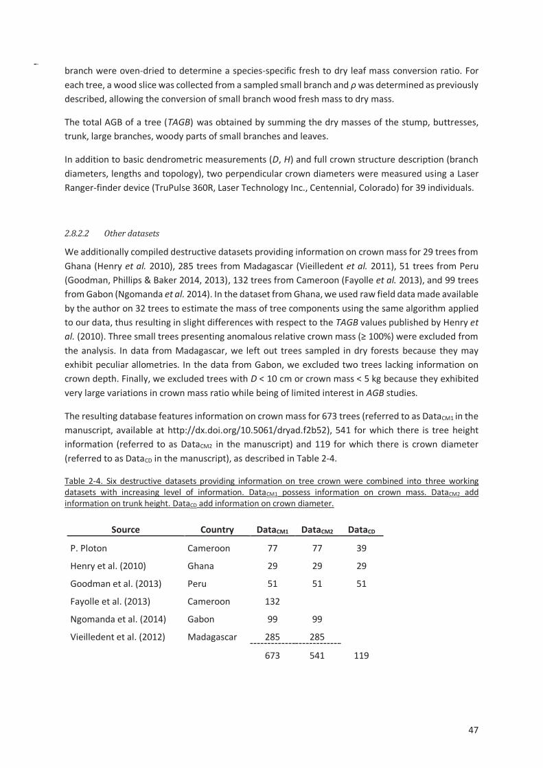
47
branch were oven-dried to determine a species-specific fresh to dry leaf mass conversion ratio. For
each tree, a wood slice was collected from a sampled small branch and ρ was determined as previously
described, allowing the conversion of small branch wood fresh mass to dry mass.
The total AGB of a tree (TAGB) was obtained by summing the dry masses of the stump, buttresses,
trunk, large branches, woody parts of small branches and leaves.
In addition to basic dendrometric measurements (D, H) and full crown structure description (branch
diameters, lengths and topology), two perpendicular crown diameters were measured using a Laser
Ranger-finder device (TruPulse 360R, Laser Technology Inc., Centennial, Colorado) for 39 individuals.
2.8.2.2 Other datasets
We additionally compiled destructive datasets providing information on crown mass for 29 trees from
Ghana (Henry et al. 2010), 285 trees from Madagascar (Vieilledent et al. 2011), 51 trees from Peru
(Goodman, Phillips & Baker 2014, 2013), 132 trees from Cameroon (Fayolle et al. 2013), and 99 trees
from Gabon (Ngomanda et al. 2014). In the dataset from Ghana, we used raw field data made available
by the author on 32 trees to estimate the mass of tree components using the same algorithm applied
to our data, thus resulting in slight differences with respect to the TAGB values published by Henry et
al. (2010). Three small trees presenting anomalous relative crown mass (≥ 100%) were excluded from
the analysis. In data from Madagascar, we left out trees sampled in dry forests because they may
exhibit peculiar allometries. In the data from Gabon, we excluded two trees lacking information on
crown depth. Finally, we excluded trees with D < 10 cm or crown mass < 5 kg because they exhibited
very large variations in crown mass ratio while being of limited interest in AGB studies.
The resulting database features information on crown mass for 673 trees (referred to as DataCM1 in the
manuscript, available at http://dx.doi.org/10.5061/dryad.f2b52), 541 for which there is tree height
information (referred to as DataCM2 in the manuscript) and 119 for which there is crown diameter
(referred to as DataCD in the manuscript), as described in Table 2-4.
Table 2-4. Six destructive datasets providing information on tree crown were combined into three working datasets with increasing level of information. DataCM1 possess information on crown mass. DataCM2 add information on trunk height. DataCD add information on crown diameter.
Source Country DataCM1 DataCM2 DataCD
P. Ploton Cameroon 77 77 39
Henry et al. (2010) Ghana 29 29 29
Goodman et al. (2013) Peru 51 51 51
Fayolle et al. (2013) Cameroon 132
Ngomanda et al. (2014) Gabon 99 99
Vieilledent et al. (2012) Madagascar 285 285
673 541 119
48
2.8.3 Inventory data
In all plots, we considered all trees with a diameter at breast height (i.e., 1.3 m or above buttresses if
present) ≥ 10 cm. In the 80 1-ha plots, tree height was measured with a Laser Ranger-finder device
(TruPulse 360R, Laser Technology Inc., Centennial, Colorado) on approximately 50 trees per plot,
homogenously distributed across diameter classes. Following Feldpausch et al. (2012), a three-
parameter Weibull function was fitted at the site level to predict height of the remaining trees: # =�*[ � ���*��!@,,. We used a relationship calibrated over two 1-ha plots near Korup to predict tree
heights in the 50-ha permanent plot. Trees were identified in the field by expert botanists, and
herbarium specimens were collected on each species per site for cross-identification at the herbarium
of Université Libre de Bruxelles (BRLU), except for Korup, where the taxonomy was confirmed at the
Missouri Botanical Garden (MO). Of 48,155 measured trees, 88.4% were identified at the species level,
4.9% at the genus level, and 0.1% at the family level, and 6.4% were left unidentified. We used the
Dryad Global Wood Density Database (Chave et al. 2009; Zanne et al. 2009) to attribute to each
individual tree a wood density value. For species known only at the genus or family level, the average
ρ value at that taxonomic level was used (Chave et al. 2006).
49
3 ASSESSING DA VINCI’S RULE ON LARGE TROPICAL
TREE CROWNS OF CONTRASTED ARCHITECTURES:
EVIDENCE FOR AREA-INCREASING BRANCHING
P. Ploton1,2, N. Barbier1,3, P. Couteron1,3, S.T. Momo1,3, S. Griffon1, B. Sonké3, U. Berger4 and R. Pélissier1
1Institut de Recherche pour le Développement, UMR AMAP, Montpellier, France 2Institut des sciences et industries du vivant et de l'environnement, Montpellier, France 3Laboratoire de Botanique systématique et d'Ecologie, Département des Sciences Biologiques, Ecole Normale Supérieure, Université de Yaoundé I, Yaoundé, Cameroon 4Technische Universität Dresden, Faculty of Environmental Sciences, Institute of Forest Growth and Forest Computer Sciences, Tharandt, Germany
3.1 Introduction
Allometric scaling relationships between tree dimensions reflect biological and physical constrains that
any tree must comply with to prevent malfunction (e.g., cavitation, buckling) as it grows in size.
Understanding the general principles that drive tree form and functions is a fascinating and vast
research topic that has been addressed from different perspectives. Given the fundamental role of
water use in trees, the focus has oftentimes been put on water transport and vascular anatomy (Tyree,
1988; Zimmermann, 1978). A renowned whole-plant model somewhat related to this theme is the Pipe
model (Shinozaki et al., 1964). The latter fundamentally stems from an observation made some 500
years ago by Leonardo da Vinci, which states that “all the branches of a tree at every stage of its height
when put together are equal in thickness to the trunk". In other words, when a parent branch splits in
i daughters, equation 1, known as area-preservation or Da Vinci’s rule, should hold on average:
� = *` '���I�}��MK_LN+ , '���^�_K�M = [� (eq. 1)
In the Pipe model, Da Vinci’s rule describes tree external architecture, which is assumed to reflect tree
hydraulic architecture. It is further posited that a unit of leaf area is supplied by a unit of conducting
tissue area, which provides a basis to study relationships between carbon allocation, photosynthetic
production and tree structural design under different conditions of stand structure or climate forcing
(Berninger and Nikinmaa, 1997; Mäkelä, 1986; Nikinmaa, 1992). Another major perspective from
which whole-plant allometric scaling have been studied is biomechanics. As every physical structure,
trees must obey some elementary physical laws, such as sustain static (self) and dynamic (wind)
loadings (Eloy, 2011; McMahon and Kronauer, 1976; Niklas, 2016). A typical example is the elastic
similarity model which considers a tree as a vertical tapering column that, in order to avoid buckling
under its own weight, must follow a number of scaling rules between column diameter, height and
mass (Niklas, 1995).
About two decades ago, the Metabolic Theory of Ecology (MTE) proposed a modelling framework
unifying hydrodynamics and biomechanics hypotheses to account for allometric scaling phenomena in
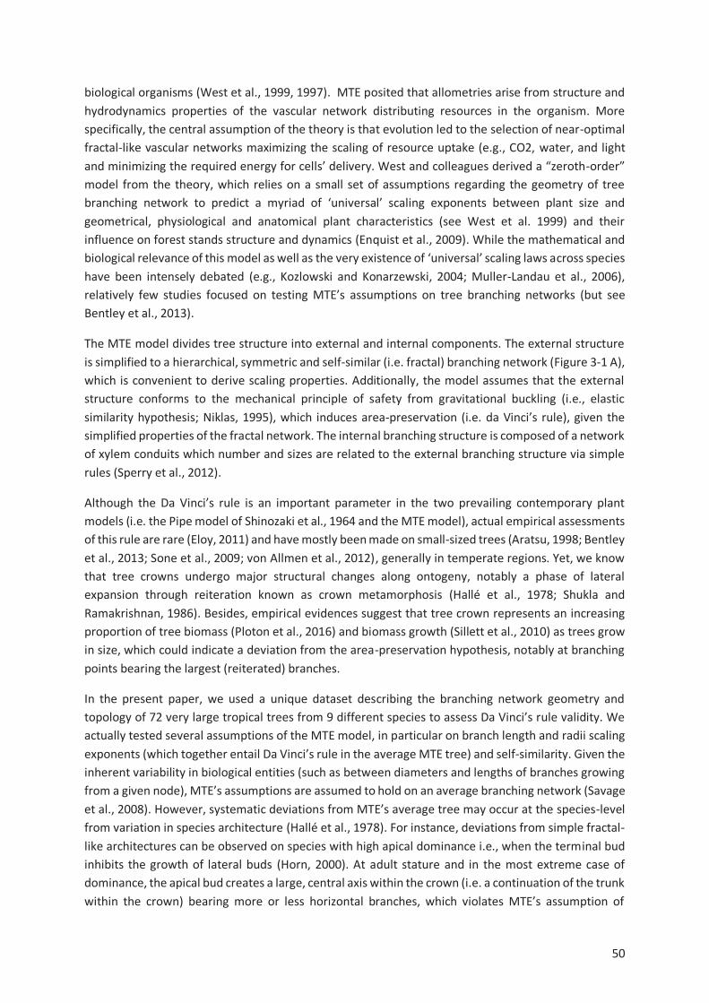
50
biological organisms (West et al., 1999, 1997). MTE posited that allometries arise from structure and
hydrodynamics properties of the vascular network distributing resources in the organism. More
specifically, the central assumption of the theory is that evolution led to the selection of near-optimal
fractal-like vascular networks maximizing the scaling of resource uptake (e.g., CO2, water, and light
and minimizing the required energy for cells’ delivery. West and colleagues derived a “zeroth-order”
model from the theory, which relies on a small set of assumptions regarding the geometry of tree
branching network to predict a myriad of ‘universal’ scaling exponents between plant size and
geometrical, physiological and anatomical plant characteristics (see West et al. 1999) and their
influence on forest stands structure and dynamics (Enquist et al., 2009). While the mathematical and
biological relevance of this model as well as the very existence of ‘universal’ scaling laws across species
have been intensely debated (e.g., Kozlowski and Konarzewski, 2004; Muller-Landau et al., 2006),
relatively few studies focused on testing MTE’s assumptions on tree branching networks (but see
Bentley et al., 2013).
The MTE model divides tree structure into external and internal components. The external structure
is simplified to a hierarchical, symmetric and self-similar (i.e. fractal) branching network (Figure 3-1 A),
which is convenient to derive scaling properties. Additionally, the model assumes that the external
structure conforms to the mechanical principle of safety from gravitational buckling (i.e., elastic
similarity hypothesis; Niklas, 1995), which induces area-preservation (i.e. da Vinci’s rule), given the
simplified properties of the fractal network. The internal branching structure is composed of a network
of xylem conduits which number and sizes are related to the external branching structure via simple
rules (Sperry et al., 2012).
Although the Da Vinci’s rule is an important parameter in the two prevailing contemporary plant
models (i.e. the Pipe model of Shinozaki et al., 1964 and the MTE model), actual empirical assessments
of this rule are rare (Eloy, 2011) and have mostly been made on small-sized trees (Aratsu, 1998; Bentley
et al., 2013; Sone et al., 2009; von Allmen et al., 2012), generally in temperate regions. Yet, we know
that tree crowns undergo major structural changes along ontogeny, notably a phase of lateral
expansion through reiteration known as crown metamorphosis (Hallé et al., 1978; Shukla and
Ramakrishnan, 1986). Besides, empirical evidences suggest that tree crown represents an increasing
proportion of tree biomass (Ploton et al., 2016) and biomass growth (Sillett et al., 2010) as trees grow
in size, which could indicate a deviation from the area-preservation hypothesis, notably at branching
points bearing the largest (reiterated) branches.
In the present paper, we used a unique dataset describing the branching network geometry and
topology of 72 very large tropical trees from 9 different species to assess Da Vinci’s rule validity. We
actually tested several assumptions of the MTE model, in particular on branch length and radii scaling
exponents (which together entail Da Vinci’s rule in the average MTE tree) and self-similarity. Given the
inherent variability in biological entities (such as between diameters and lengths of branches growing
from a given node), MTE’s assumptions are assumed to hold on an average branching network (Savage
et al., 2008). However, systematic deviations from MTE’s average tree may occur at the species-level
from variation in species architecture (Hallé et al., 1978). For instance, deviations from simple fractal-
like architectures can be observed on species with high apical dominance i.e., when the terminal bud
inhibits the growth of lateral buds (Horn, 2000). At adult stature and in the most extreme case of
dominance, the apical bud creates a large, central axis within the crown (i.e. a continuation of the trunk
within the crown) bearing more or less horizontal branches, which violates MTE’s assumption of
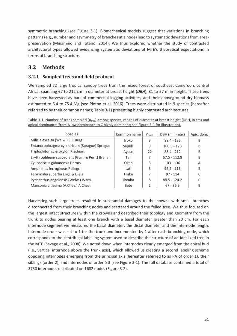
51
symmetric branching (see Figure 3-1). Biomechanical models suggest that variations in branching
patterns (e.g., number and asymmetry of branches at a node) lead to systematic deviations from area-
preservation (Minamino and Tateno, 2014). We thus explored whether the study of contrasted
architectural types allowed evidencing systematic deviations of MTE’s theoretical expectations in
terms of branching structure.
3.2 Methods
3.2.1 Sampled trees and field protocol
We sampled 72 large tropical canopy trees from the mixed forest of southeast Cameroon, central
Africa, spanning 67 to 212 cm in diameter at breast height (DBH), 31 to 57 m in height. These trees
have been harvested as part of commercial logging activities, and their aboveground dry biomass
estimated to 5.4 to 75.4 Mg (see Ploton et al. 2016). Trees were distributed in 9 species (hereafter
referred to by their common names; Table 3-1) presenting highly contrasted architectures.
Table 3-1. Number of trees sampled (ntree) among species, ranges of diameter at breast height (DBH, in cm) and apical dominance (from A low dominance to C highly dominant; see Figure 3-1 for illustration).
Species Common name ntree DBH (min-max) Apic. dom.
Milicia excelsa (Welw.) C.C.Berg Iroko 9 88.4 - 126 B
Entandrophragma cylindricum (Sprague) Sprague Sapelli 9 100.5 - 178 B
Triplochiton scleroxylon K.Schum. Ayous 22 88.4 - 212 B
Erythrophleum suaveolens (Guill. & Perr.) Brenan Tali 7 67.5 - 112.8 B
Cylicodiscus gabunensis Harms Okan 5 103 - 136 A
Amphimas ferrugineus Pellegr. Lati 3 92.5 - 113 B
Terminalia superba Engl. & Diels Frake 7 97 - 114 C
Pycnanthus angolensis (Welw.) Warb. Ilomba 8 88.5 - 124.2 C
Mansonia altissima (A.Chev.) A.Chev. Bete 2 67 - 86.5 B
Harvesting such large trees resulted in substantial damages to the crowns with small branches
disconnected from their branching nodes and scattered around the felled tree. We thus focused on
the largest intact structures within the crowns and described their topology and geometry from the
trunk to nodes bearing at least one branch with a basal diameter greater than 20 cm. For each
internode segment we measured the basal diameter, the distal diameter and the internode length.
Internode order was set to 1 for the trunk and incremented by 1 after each branching node, which
corresponds to the centrifugal labelling system used to describe the structure of an idealized tree in
the MTE (Savage et al., 2008). We noted down when internodes clearly emerged from the apical bud
(i.e., vertical internode above the trunk axis), which allowed us creating a second labeling scheme
opposing internodes emerging from the principal axis (hereafter referred to as PA of order 1), their
siblings (order 2), and internodes of order ≥ 3 (see Figure 3-1). The full database contained a total of
3730 internodes distributed on 1682 nodes (Figure 3-2).
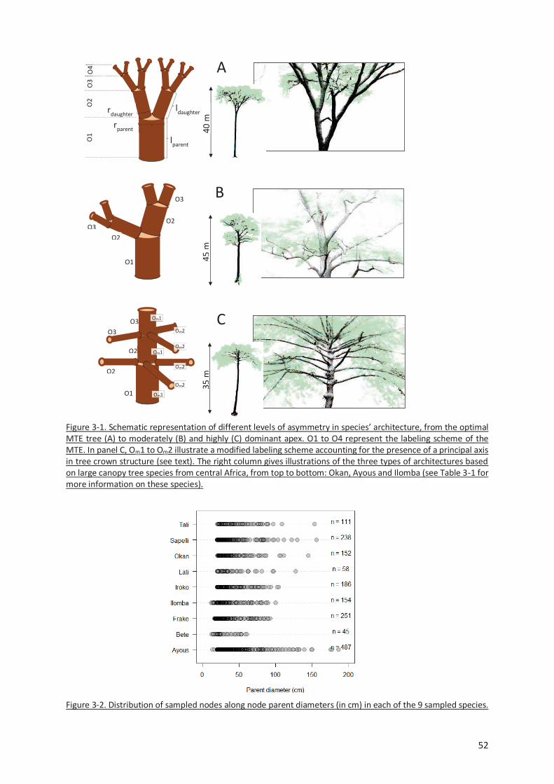
52
Figure 3-1. Schematic representation of different levels of asymmetry in species’ architecture, from the optimal MTE tree (A) to moderately (B) and highly (C) dominant apex. O1 to O4 represent the labeling scheme of the MTE. In panel C, Om1 to Om2 illustrate a modified labeling scheme accounting for the presence of a principal axis in tree crown structure (see text). The right column gives illustrations of the three types of architectures based on large canopy tree species from central Africa, from top to bottom: Okan, Ayous and Ilomba (see Table 3-1 for more information on these species).
Figure 3-2. Distribution of sampled nodes along node parent diameters (in cm) in each of the 9 sampled species.
40 m
45
m
35 m
lparent
ldaughter
rparent
rdaughter
O1
O2
O3 O
4
O1
O2
A
B
C
O3
O1
O2
O2
O3 O3
O2
O3
Om1
Om1
Om1
Om2
Om2
Om2
Om2
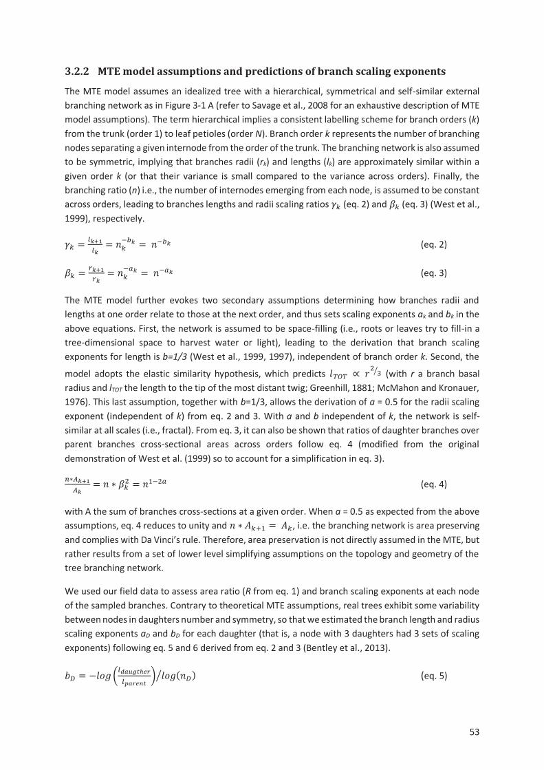
53
3.2.2 MTE model assumptions and predictions of branch scaling exponents
The MTE model assumes an idealized tree with a hierarchical, symmetrical and self-similar external
branching network as in Figure 3-1 A (refer to Savage et al., 2008 for an exhaustive description of MTE
model assumptions). The term hierarchical implies a consistent labelling scheme for branch orders (k)
from the trunk (order 1) to leaf petioles (order N). Branch order k represents the number of branching
nodes separating a given internode from the order of the trunk. The branching network is also assumed
to be symmetric, implying that branches radii (rk) and lengths (lk) are approximately similar within a
given order k (or that their variance is small compared to the variance across orders). Finally, the
branching ratio (n) i.e., the number of internodes emerging from each node, is assumed to be constant
across orders, leading to branches lengths and radii scaling ratios �� (eq. 2) and 7� (eq. 3) (West et al.,
1999), respectively.
�� = ���y�� = ��W�� =0�W�� (eq. 2)
7� = _��y_� = ��W�� =0�W�� (eq. 3)
The MTE model further evokes two secondary assumptions determining how branches radii and
lengths at one order relate to those at the next order, and thus sets scaling exponents ak and bk in the
above equations. First, the network is assumed to be space-filling (i.e., roots or leaves try to fill-in a
tree-dimensional space to harvest water or light), leading to the derivation that branch scaling
exponents for length is b=1/3 (West et al., 1999, 1997), independent of branch order k. Second, the
model adopts the elastic similarity hypothesis, which predicts �|�| 0� 0 �+ �� (with r a branch basal
radius and lTOT the length to the tip of the most distant twig; Greenhill, 1881; McMahon and Kronauer,
1976). This last assumption, together with b=1/3, allows the derivation of a = 0.5 for the radii scaling
exponent (independent of k) from eq. 2 and 3. With a and b independent of k, the network is self-
similar at all scales (i.e., fractal). From eq. 3, it can also be shown that ratios of daughter branches over
parent branches cross-sectional areas across orders follow eq. 4 (modified from the original
demonstration of West et al. (1999) so to account for a simplification in eq. 3).
�"���y�� = � " 7�+ = ��W+� (eq. 4)
with A the sum of branches cross-sections at a given order. When a = 0.5 as expected from the above
assumptions, eq. 4 reduces to unity and � " '�E� =0'�, i.e. the branching network is area preserving
and complies with Da Vinci’s rule. Therefore, area preservation is not directly assumed in the MTE, but
rather results from a set of lower level simplifying assumptions on the topology and geometry of the
tree branching network.
We used our field data to assess area ratio (R from eq. 1) and branch scaling exponents at each node
of the sampled branches. Contrary to theoretical MTE assumptions, real trees exhibit some variability
between nodes in daughters number and symmetry, so that we estimated the branch length and radius
scaling exponents aD and bD for each daughter (that is, a node with 3 daughters had 3 sets of scaling
exponents) following eq. 5 and 6 derived from eq. 2 and 3 (Bentley et al., 2013).
�� = ����O�� ¡¢S£Q¤�¥ ¤Q¦S Z ���0*��,� (eq. 5)
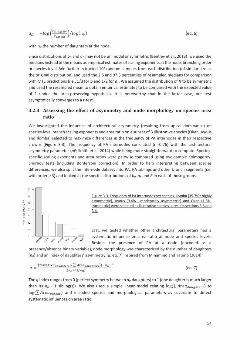
54
�� = ����O_� ¡¢S£Q¤_¥ ¤Q¦S Z ���*��,� (eq. 6)
with nD the number of daughters at the node.
Since distributions of bD and aD may not be unimodal or symmetric (Bentley et al., 2013), we used the
medians instead of the means as empirical estimates of scaling exponents at the node, branching order
or species level. We further extracted 104 random samples from each distribution (of similar size as
the original distribution) and used the 2.5 and 97.5 percentiles of resampled medians for comparison
with MTE predictions (i.e., 1/3 for b and 1/2 for a). We assumed the distribution of R to be symmetric
and used the resampled mean to obtain empirical estimates to be compared with the expected value
of 1 under the area-preserving hypothesis. It is noteworthy that in the latter case, our test
asymptotically converges to a t-test.
3.2.3 Assessing the effect of asymmetry and node morphology on species area
ratio
We investigated the influence of architectural asymmetry (resulting from apical dominance) on
species-level branch scaling exponents and area ratio on a subset of 3 illustrative species (Okan, Ayous
and Ilomba) selected to maximize differences in the frequency of PA internodes in their respective
crowns (Figure 3-3). The frequency of PA internodes correlated (r=-0.76) with the architectural
asymmetry parameter (pF; Smith et al. 2014) while being more straightforward to compute. Species-
specific scaling exponents and area ratios were pairwise-compared using two-sample Kolmogorov-
Smirnov tests (including Bonferroni correction). In order to help interpreting between species
differences, we also split the internode dataset into PA, PA siblings and other branch segments (i.e.
with order ≥ 3) and looked at the specific distributions of bb, ab and R in each of those groups.
Figure 3-3. Frequency of PA internodes per species. Ilomba (35.7% : highly asymmetric), Ayous (9.4% : moderately asymmetric) and Okan (1.3%: symmetric) were selected as illustrative species in results sections 3.3 and 3.4.
Last, we tested whether other architectural parameters had a
systematic influence on area ratio at node and species levels.
Besides the presence of PA at a node (encoded as a
presence/absence binary variable), node morphology was characterized by the number of daughters
(nD) and an index of daughters’ asymmetry (q, eq. 7) inspired from Minamino and Tateno (2014):
§ = ¨©ª«0*�_K�� ¡¢£SQ¤R, ¨`�_K�� ¡¢£SQ¤R¬ ¬W0�®¯y**�®W�, �® , (eq. 7)
The q index ranges from 0 (perfect symmetry between nD daughters) to 1 (one daughter is much larger
than its nD - 1 sibling(s)). We also used a simple linear model relating l°±0*`'���I�}��MK_L, to
l°±0*` '���^�_K�M, and included species and morphological parameters as covariate to detect
systematic influences on area ratio.
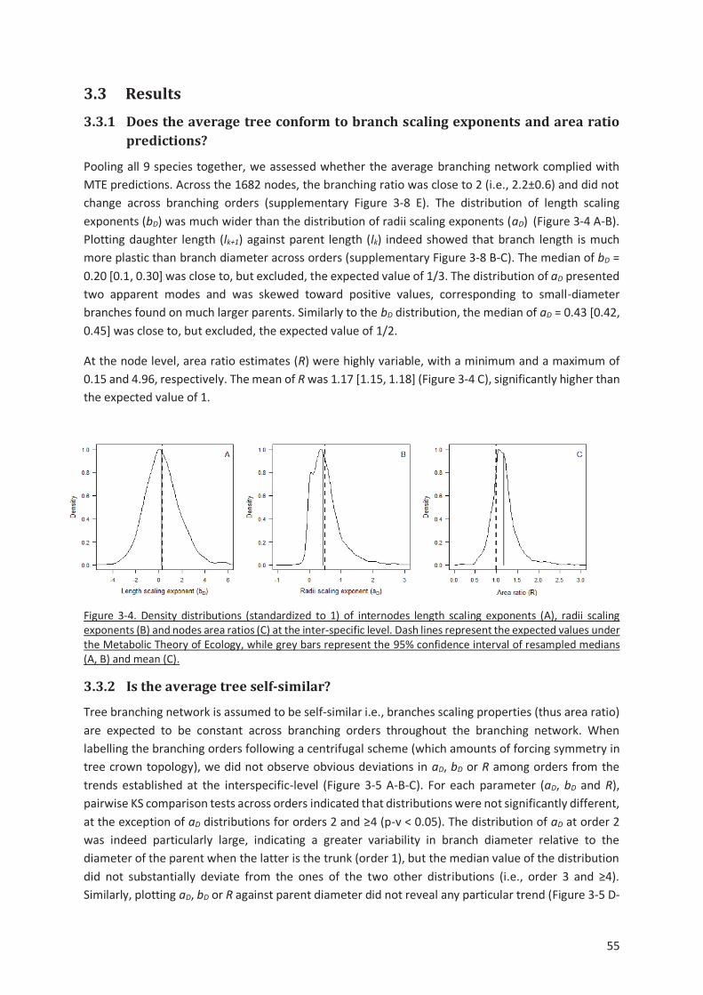
55
3.3 Results
3.3.1 Does the average tree conform to branch scaling exponents and area ratio
predictions?
Pooling all 9 species together, we assessed whether the average branching network complied with
MTE predictions. Across the 1682 nodes, the branching ratio was close to 2 (i.e., 2.2±0.6) and did not
change across branching orders (supplementary Figure 3-8 E). The distribution of length scaling
exponents (bD) was much wider than the distribution of radii scaling exponents (aD) (Figure 3-4 A-B).
Plotting daughter length (lk+1) against parent length (lk) indeed showed that branch length is much
more plastic than branch diameter across orders (supplementary Figure 3-8 B-C). The median of bD =
0.20 [0.1, 0.30] was close to, but excluded, the expected value of 1/3. The distribution of aD presented
two apparent modes and was skewed toward positive values, corresponding to small-diameter
branches found on much larger parents. Similarly to the bD distribution, the median of aD = 0.43 [0.42,
0.45] was close to, but excluded, the expected value of 1/2.
At the node level, area ratio estimates (R) were highly variable, with a minimum and a maximum of
0.15 and 4.96, respectively. The mean of R was 1.17 [1.15, 1.18] (Figure 3-4 C), significantly higher than
the expected value of 1.
Figure 3-4. Density distributions (standardized to 1) of internodes length scaling exponents (A), radii scaling exponents (B) and nodes area ratios (C) at the inter-specific level. Dash lines represent the expected values under the Metabolic Theory of Ecology, while grey bars represent the 95% confidence interval of resampled medians (A, B) and mean (C).
3.3.2 Is the average tree self-similar?
Tree branching network is assumed to be self-similar i.e., branches scaling properties (thus area ratio)
are expected to be constant across branching orders throughout the branching network. When
labelling the branching orders following a centrifugal scheme (which amounts of forcing symmetry in
tree crown topology), we did not observe obvious deviations in aD, bD or R among orders from the
trends established at the interspecific-level (Figure 3-5 A-B-C). For each parameter (aD, bD and R),
pairwise KS comparison tests across orders indicated that distributions were not significantly different,
at the exception of aD distributions for orders 2 and ≥4 (p-v < 0.05). The distribution of aD at order 2
was indeed particularly large, indicating a greater variability in branch diameter relative to the
diameter of the parent when the latter is the trunk (order 1), but the median value of the distribution
did not substantially deviate from the ones of the two other distributions (i.e., order 3 and ≥4).
Similarly, plotting aD, bD or R against parent diameter did not reveal any particular trend (Figure 3-5 D-
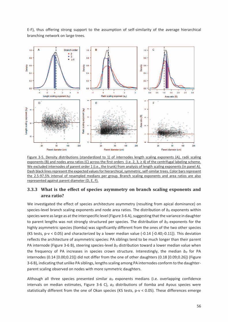
56
E-F), thus offering strong support to the assumption of self-similarity of the average hierarchical
branching network on large trees.
Figure 3-5. Density distributions (standardized to 1) of internodes length scaling exponents (A), radii scaling exponents (B) and nodes area ratios (C) across the first orders (i.e. 2, 3, ≥ 4) of the centrifugal labeling scheme. We excluded internodes of parent order 1 (i.e., the trunk) from analysis of length scaling exponents (in panel A). Dash black lines represent the expected values for hierarchical, symmetric, self-similar trees. Color bars represent the 2.5-97.5% interval of resampled medians per group. Branch scaling exponents and area ratios are also represented against parent diameter (D, E, F).
3.3.3 What is the effect of species asymmetry on branch scaling exponents and
area ratio?
We investigated the effect of species architecture asymmetry (resulting from apical dominance) on
species-level branch scaling exponents and node area ratios. The distribution of bD exponents within
species were as large as at the interspecific level (Figure 3-6 A), suggesting that the variance in daughter
to parent lengths was not strongly structured per species. The distribution of bD exponents for the
highly asymmetric species (Ilomba) was significantly different from the ones of the two other species
(KS tests, p-v < 0.05) and characterized by a lower median value (-0.14 [-0.40;-0.11]). This deviation
reflects the architecture of asymmetric species: PA siblings tend to be much longer than their parent
PA internode (Figure 3-6 B), steering species-level bD distribution toward a lower median value when
the frequency of PA increases in species crown structure. Interestingly, the median bD for PA
internodes (0.14 [0.00;0.23]) did not differ from the one of other daughters (0.18 [0.09;0.26]) (Figure
3-6 B), indicating that unlike PA siblings, lengths scaling among PA internodes conform to the daughter-
parent scaling observed on nodes with more symmetric daughters.
Although all three species presented similar aD exponents medians (i.e. overlapping confidence
intervals on median estimates, Figure 3-6 C), aD distributions of Ilomba and Ayous species were
statistically different from the one of Okan species (KS tests, p-v < 0.05). These differences emerge
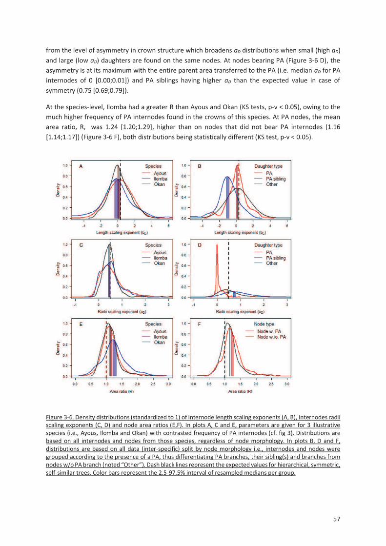
57
from the level of asymmetry in crown structure which broadens aD distributions when small (high aD)
and large (low aD) daughters are found on the same nodes. At nodes bearing PA (Figure 3-6 D), the
asymmetry is at its maximum with the entire parent area transferred to the PA (i.e. median aD for PA
internodes of 0 [0.00;0.01]) and PA siblings having higher aD than the expected value in case of
symmetry (0.75 [0.69;0.79]).
At the species-level, Ilomba had a greater R than Ayous and Okan (KS tests, p-v < 0.05), owing to the
much higher frequency of PA internodes found in the crowns of this species. At PA nodes, the mean
area ratio, R, was 1.24 [1.20;1.29], higher than on nodes that did not bear PA internodes (1.16
[1.14;1.17]) (Figure 3-6 F), both distributions being statistically different (KS test, p-v < 0.05).
Figure 3-6. Density distributions (standardized to 1) of internode length scaling exponents (A, B), internodes radii scaling exponents (C, D) and node area ratios (E,F). In plots A, C and E, parameters are given for 3 illustrative species (i.e., Ayous, Ilomba and Okan) with contrasted frequency of PA internodes (cf. fig 3). Distributions are based on all internodes and nodes from those species, regardless of node morphology. In plots B, D and F, distributions are based on all data (inter-specific) split by node morphology i.e., internodes and nodes were grouped according to the presence of a PA, thus differentiating PA branches, their sibling(s) and branches from nodes w/o PA branch (noted “Other”). Dash black lines represent the expected values for hierarchical, symmetric,
self-similar trees. Color bars represent the 2.5-97.5% interval of resampled medians per group.
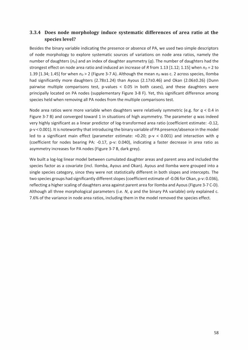
58
3.3.4 Does node morphology induce systematic differences of area ratio at the
species level?
Besides the binary variable indicating the presence or absence of PA, we used two simple descriptors
of node morphology to explore systematic sources of variations on node area ratios, namely the
number of daughters (nD) and an index of daughter asymmetry (q). The number of daughters had the
strongest effect on node area ratio and induced an increase of R from 1.13 [1.12; 1.15] when nD = 2 to
1.39 [1.34; 1.45] for when nD > 2 (Figure 3-7 A). Although the mean nD was c. 2 across species, Ilomba
had significantly more daughters (2.78±1.24) than Ayous (2.17±0.46) and Okan (2.06±0.26) (Dunn
pairwise multiple comparisons test, p-values < 0.05 in both cases), and these daughters were
principally located on PA nodes (supplementary Figure 3-8 F). Yet, this significant difference among
species held when removing all PA nodes from the multiple comparisons test.
Node area ratios were more variable when daughters were relatively symmetric (e.g. for q < 0.4 in
Figure 3-7 B) and converged toward 1 in situations of high asymmetry. The parameter q was indeed
very highly significant as a linear predictor of log-transformed area ratio (coefficient estimate: -0.12,
p-v < 0.001). It is noteworthy that introducing the binary variable of PA presence/absence in the model
led to a significant main effect (parameter estimate: +0.20; p-v < 0.001) and interaction with q
(coefficient for nodes bearing PA: -0.17, p-v: 0.040), indicating a faster decrease in area ratio as
asymmetry increases for PA nodes (Figure 3-7 B, dark grey).
We built a log-log linear model between cumulated daughter areas and parent area and included the
species factor as a covariate (incl. Ilomba, Ayous and Okan). Ayous and Ilomba were grouped into a
single species category, since they were not statistically different in both slopes and intercepts. The
two species groups had significantly different slopes (coefficient estimate of -0.06 for Okan, p-v: 0.036),
reflecting a higher scaling of daughters area against parent area for Ilomba and Ayous (Figure 3-7 C-D).
Although all three morphological parameters (i.e. N, q and the binary PA variable) only explained c.
7.6% of the variance in node area ratios, including them in the model removed the species effect.
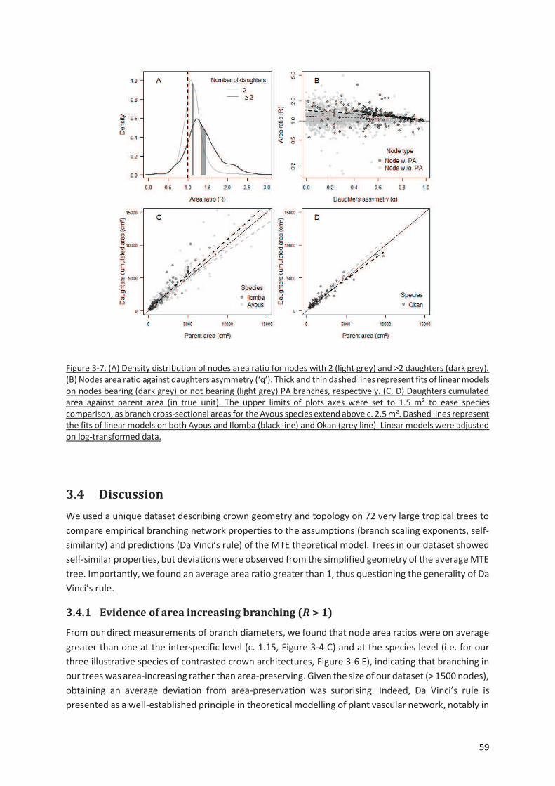
59
Figure 3-7. (A) Density distribution of nodes area ratio for nodes with 2 (light grey) and >2 daughters (dark grey). (B) Nodes area ratio against daughters asymmetry (‘q’). Thick and thin dashed lines represent fits of linear models on nodes bearing (dark grey) or not bearing (light grey) PA branches, respectively. (C, D) Daughters cumulated area against parent area (in true unit). The upper limits of plots axes were set to 1.5 m² to ease species comparison, as branch cross-sectional areas for the Ayous species extend above c. 2.5 m². Dashed lines represent the fits of linear models on both Ayous and Ilomba (black line) and Okan (grey line). Linear models were adjusted on log-transformed data.
3.4 Discussion
We used a unique dataset describing crown geometry and topology on 72 very large tropical trees to
compare empirical branching network properties to the assumptions (branch scaling exponents, self-
similarity) and predictions (Da Vinci’s rule) of the MTE theoretical model. Trees in our dataset showed
self-similar properties, but deviations were observed from the simplified geometry of the average MTE
tree. Importantly, we found an average area ratio greater than 1, thus questioning the generality of Da
Vinci’s rule.
3.4.1 Evidence of area increasing branching (R > 1)
From our direct measurements of branch diameters, we found that node area ratios were on average
greater than one at the interspecific level (c. 1.15, Figure 3-4 C) and at the species level (i.e. for our
three illustrative species of contrasted crown architectures, Figure 3-6 E), indicating that branching in
our trees was area-increasing rather than area-preserving. Given the size of our dataset (> 1500 nodes),
obtaining an average deviation from area-preservation was surprising. Indeed, Da Vinci’s rule is
presented as a well-established principle in theoretical modelling of plant vascular network, notably in
60
the MTE model (Enquist, 2002; West et al., 1999) and, as far as we know, it has never been questioned
in MTE’s model extensions (e.g. Smith et al., 2014; Sperry et al., 2012; von Allmen et al., 2012) and
MTE-like models (e.g. Savage et al., 2010). The majority of empirical assessments of this rule have
indeed reported area ratios varying around a situation of area-preservation (e.g. Bentley et al., 2013;
MacFarlane et al., 2014). Yet, a survey of the literature shows that the Da Vinci’s rule has not been
extensively assessed (Eloy, 2011) and that in most cases, empirical studies were based on few
individuals (typically less than 5) of small size (typically less than c. 15 cm D) (e.g. Bentley et al., 2013;
Bertram, 1989; McMahon and Kronauer, 1976; Tredennick et al., 2013). Besides, empirical
assessments are not univocal (Aratsu, 1998; Minamino and Tateno, 2014; Yamamoto and Kobayashi,
1993). Aratsu (1998) for instance, whose dataset stands out by its unusual number of large branches
(> 20 cm of basal diameter), found that 9 out of 10 temperate tree species actually showed area
increasing branching. The results of the present study further question the generality of Da Vinci’s rule
and clearly show that more research efforts should be made to assess R on trees of different sizes,
species and regions of the world.
An important issue when sampling area ratio is the location at which branch diameter is measured,
which is not defined in the Da Vinci’s rule. Minamino and Tateno (2014) indeed showed that if the
branching network maintains elastic similarity, branch taper should be smooth away from
ramifications but change markedly before and after a branching point, leading to R > 1 when the
distance from the point of measurement of branches diameter and the branching point is virtually null.
Although we measured branch diameters at reasonable distances from branching points so to avoid
the obvious swelling occurring bellow and above large branches ramification, our results (R > 1) could
reflect this asymmetry in parent and daughters local tapers. More generally, disagreements between
empirical assessments of Da Vinci’s rule may come from differences in field protocols (i.e. use of distal
parent diameter and basal daughters’ diameter vs use of mid-branch diameters).
3.4.2 Sources of variation of the node area ratio
Regardless of the organization of branches in a tree, if branch scaling properties are homogeneous (i.e.
regular allometry between branch diameter and length) and if the tree conforms to Da Vinci’s rule,
then whole-tree volume (or biomass, assuming homogeneous wood density) may be roughly
approximated by the volume of a cylinder (Horn, 2000). Under the assumption of homogeneous
branch scaling properties, the average area ratio thus has direct consequence on whole-tree volume
and biomass scaling. Identifying systematic sources of variation of R associated to particular node
morphologies would give us a point of departure for further analyses, such as the covariation between
daughters dimensions (length, taper) and R in particular nodes configuration, and may provide
valuable insights into how tree species could be grouped to improve allometric scaling predictions,
notably on tree biomass.
Because empirical studies suggest an increase of crown mass relative to total tree mass on large
tropical canopy trees (Ploton et al., 2016), an intuitive hypothesis was that R may increase on those
trees, notably on the largest branches in tree crowns following structural changes associated to crown
metamorphosis. Our data does not support this hypothesis. On the full dataset (interspecific level), R
was higher than one on the entire range of branch size and did not show marked variation pattern on
large-diameter branches (Figure 3-5 E).Species and individual-tree factors also weakly explain R
variability (c. 2% and c. 7%, respectively), which illustrate the convergence of species (and trees)
vascular networks to similar structural properties (from the view point of R frequency distributions) as
61
they share the same purposes (e.g. water transport) and constraints (hydraulic, mechanical). Most of
R variability occurred at the node level, and a similar pattern of variance partitioning can be expected
for branch scaling exponents (i.e. among different species and trees, most of the variability in diameter
– length or diameter –mass scaling exponents is found at the branch level, Tredennick et al., 2013). We
emphasize that even if two trees present similar frequency distributions of R (or branch scaling
exponents), between-trees variation in branching pattern (architecture) may have important impact
on the overall tree volume and mass, because e.g. deviation from R = 1 on a large or a small branch
have a very different impact on whole-tree volume. Our analyses showed that node morphology (as
described by nD, q and the PA binary variable) have a systematic influence on node level R. The different
trends that we uncovered all fall in line with the predictions of Minamino and Tateno (2014) based on
mechanical calculations, suggesting that the maintenance of mechanical stability could be at the origin
of our observations. It should be noted, however, that the three morphological parameters together
explained less than 10% of node level R variation. Hereafter, we provide tentative interpretations of
our findings.
First, we found that the average R increased substantially with the number of daughters ND (Figure 3-7
A). Among the three species illustrating contrasting levels of apical dominance (hence architectural
asymmetry), ND was higher on average (c. 2.5-3) and more variable on the Ilomba species (highly
asymmetric architecture) and appeared to converge toward nD = 2 as the symmetry of crown
architecture increased (fig S1 F). This structural trend could reflect species growth strategies. The high
apical dominance is usually interpreted as a trait favoring faster height growth, a competitive
advantage typically associated to pioneer species. Apical dominance also creates multi-layered crowns
that are more efficient in harvesting light in bright (top-of-the-canopy) conditions. In contrast, low
apical dominance (symmetric architecture) creates a mono-layered crown that minimizes self-shading,
a characteristic deemed more efficient in shaded conditions (Horn, 2000, 1971). Following this trait,
our three illustrative species could be ranked from pioneer-like (Ilomba) to shade tolerant-like (Okan)
species (Figure 3-3 3). It is commonly acknowledge that fast growing pioneer species tend to have
lighter wood (c. 0.41 g.cm3 for Ilomba) than slow-growing shade tolerant species (c. 0.79 g.cm3 for
Okan). Hence, we hypothesize that the higher and more variable nD observed on Ilomba than Okan
could reflect a more opportunistic strategy of light harvesting, as the cost associated to growing (and
shedding) daughters is lower on this species.
Second, we found that PA nodes (which compose the vertical, central axis of the crown) had a higher
R on average (Figure 3-6 F). Conversely, R decreased with increasing asymmetry between daughters
(parameter q, Figure 3-7 B). These two results may appear contradictory, because PA daughters are
instinctively thought as being highly dominant over their siblings (i.e. leading to a high q). Figure 3-7 B
shows that this is not necessarily the case: a PA daughter can have a diameter relatively close to that
of its siblings (low q), in which case nodes reached particularly high R values. For those nodes (bearing
a PA daughter), R converged faster toward 1 with increasing asymmetry (i.e. steeper decreasing slope
in Figure 3-7 B). The overall variation pattern of R with nD, PA and q may be interpreted as an ageing
process. Sone et al. (2009, 2005) have shown that the sum of growth areas of daughter branches was
higher than parent growth area on two Acer species, so that nodes that did not experience shedding
had R > 1 and shedding was necessary to conform to Da Vinci’s rule. Variability of R values within a
crown may thus represent diverse states of modification of nodes morphology that temporarily
conform to Da Vinci’s rule (Minamino and Tateno, 2014). On species that present a principal axis (PA)
up to the top of the crown such as Ilomba, relatively young nodes found at the crown-top bear
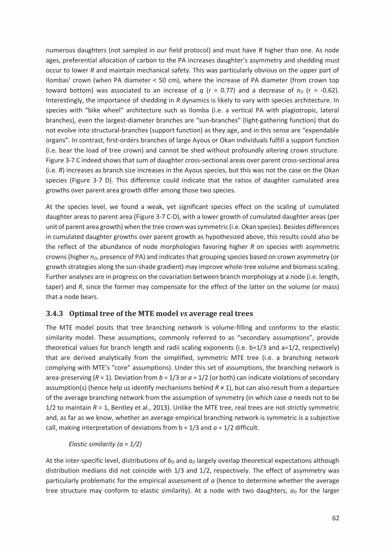
62
numerous daughters (not sampled in our field protocol) and must have R higher than one. As node
ages, preferential allocation of carbon to the PA increases daughter’s asymmetry and shedding must
occur to lower R and maintain mechanical safety. This was particularly obvious on the upper part of
Ilombas’ crown (when PA diameter < 50 cm), where the increase of PA diameter (from crown top
toward bottom) was associated to an increase of q (r = 0.77) and a decrease of nD (r = -0.62).
Interestingly, the importance of shedding in R dynamics is likely to vary with species architecture. In
species with “bike wheel” architecture such as Ilomba (i.e. a vertical PA with plagiotropic, lateral
branches), even the largest-diameter branches are “sun-branches” (light-gathering function) that do
not evolve into structural-branches (support function) as they age, and in this sense are “expendable
organs”. In contrast, first-orders branches of large Ayous or Okan individuals fulfill a support function
(i.e. bear the load of tree crown) and cannot be shed without profoundly altering crown structure.
Figure 3-7 C indeed shows that sum of daughter cross-sectional areas over parent cross-sectional area
(i.e. R) increases as branch size increases in the Ayous species, but this was not the case on the Okan
species (Figure 3-7 D). This difference could indicate that the ratios of daughter cumulated area
growths over parent area growth differ among those two species.
At the species level, we found a weak, yet significant species effect on the scaling of cumulated
daughter areas to parent area (Figure 3-7 C-D), with a lower growth of cumulated daughter areas (per
unit of parent area growth) when the tree crown was symmetric (i.e. Okan species). Besides differences
in cumulated daughter growths over parent growth as hypothesized above, this results could also be
the reflect of the abundance of node morphologies favoring higher R on species with asymmetric
crowns (higher nD, presence of PA) and indicates that grouping species based on crown asymmetry (or
growth strategies along the sun-shade gradient) may improve whole-tree volume and biomass scaling.
Further analyses are in progress on the covariation between branch morphology at a node (i.e. length,
taper) and R, since the former may compensate for the effect of the latter on the volume (or mass)
that a node bears.
3.4.3 Optimal tree of the MTE model vs average real trees
The MTE model posits that tree branching network is volume-filling and conforms to the elastic
similarity model. These assumptions, commonly referred to as “secondary assumptions”, provide
theoretical values for branch length and radii scaling exponents (i.e. b=1/3 and a=1/2, respectively)
that are derived analytically from the simplified, symmetric MTE tree (i.e. a branching network
complying with MTE’s “core” assumptions). Under this set of assumptions, the branching network is
area-preserving (R = 1). Deviation from b = 1/3 or a = 1/2 (or both) can indicate violations of secondary
assumption(s) (hence help us identify mechanisms behind R ≠ 1), but can also result from a departure
of the average branching network from the assumption of symmetry (in which case a needs not to be
1/2 to maintain R = 1, Bentley et al., 2013). Unlike the MTE tree, real trees are not strictly symmetric
and, as far as we know, whether an average empirical branching network is symmetric is a subjective
call, making interpretation of deviations from b = 1/3 and a = 1/2 difficult.
Elastic similarity (a = 1/2)
At the inter-specific level, distributions of bD and aD largely overlap theoretical expectations although
distribution medians did not coincide with 1/3 and 1/2, respectively. The effect of asymmetry was
particularly problematic for the empirical assessment of a (hence to determine whether the average
tree structure may conform to elastic similarity). At a node with two daughters, aD for the larger
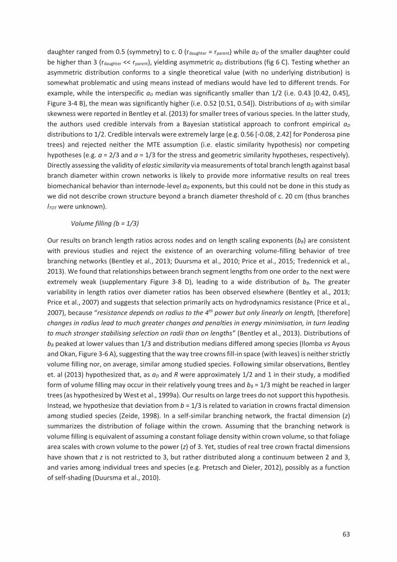
63
daughter ranged from 0.5 (symmetry) to c. 0 (rdaughter = rparent) while aD of the smaller daughter could
be higher than 3 (rdaughter << rparent), yielding asymmetric aD distributions (fig 6 C). Testing whether an
asymmetric distribution conforms to a single theoretical value (with no underlying distribution) is
somewhat problematic and using means instead of medians would have led to different trends. For
example, while the interspecific aD median was significantly smaller than 1/2 (i.e. 0.43 [0.42, 0.45],
Figure 3-4 B), the mean was significantly higher (i.e. 0.52 [0.51, 0.54]). Distributions of aD with similar
skewness were reported in Bentley et al. (2013) for smaller trees of various species. In the latter study,
the authors used credible intervals from a Bayesian statistical approach to confront empirical aD
distributions to 1/2. Credible intervals were extremely large (e.g. 0.56 [-0.08, 2.42] for Ponderosa pine
trees) and rejected neither the MTE assumption (i.e. elastic similarity hypothesis) nor competing
hypotheses (e.g. a = 2/3 and a = 1/3 for the stress and geometric similarity hypotheses, respectively).
Directly assessing the validity of elastic similarity via measurements of total branch length against basal
branch diameter within crown networks is likely to provide more informative results on real trees
biomechanical behavior than internode-level aD exponents, but this could not be done in this study as
we did not describe crown structure beyond a branch diameter threshold of c. 20 cm (thus branches
lTOT were unknown).
Volume filling (b = 1/3)
Our results on branch length ratios across nodes and on length scaling exponents (bB) are consistent
with previous studies and reject the existence of an overarching volume-filling behavior of tree
branching networks (Bentley et al., 2013; Duursma et al., 2010; Price et al., 2015; Tredennick et al.,
2013). We found that relationships between branch segment lengths from one order to the next were
extremely weak (supplementary Figure 3-8 D), leading to a wide distribution of bB. The greater
variability in length ratios over diameter ratios has been observed elsewhere (Bentley et al., 2013;
Price et al., 2007) and suggests that selection primarily acts on hydrodynamics resistance (Price et al.,
2007), because “resistance depends on radius to the 4th power but only linearly on length, [therefore]
changes in radius lead to much greater changes and penalties in energy minimisation, in turn leading
to much stronger stabilising selection on radii than on lengths” (Bentley et al., 2013). Distributions of
bB peaked at lower values than 1/3 and distribution medians differed among species (Ilomba vs Ayous
and Okan, Figure 3-6 A), suggesting that the way tree crowns fill-in space (with leaves) is neither strictly
volume filling nor, on average, similar among studied species. Following similar observations, Bentley
et. al (2013) hypothesized that, as aD and R were approximately 1/2 and 1 in their study, a modified
form of volume filling may occur in their relatively young trees and bB = 1/3 might be reached in larger
trees (as hypothesized by West et al., 1999a). Our results on large trees do not support this hypothesis.
Instead, we hypothesize that deviation from b = 1/3 is related to variation in crowns fractal dimension
among studied species (Zeide, 1998). In a self-similar branching network, the fractal dimension (z)
summarizes the distribution of foliage within the crown. Assuming that the branching network is
volume filling is equivalent of assuming a constant foliage density within crown volume, so that foliage
area scales with crown volume to the power (z) of 3. Yet, studies of real tree crown fractal dimensions
have shown that z is not restricted to 3, but rather distributed along a continuum between 2 and 3,
and varies among individual trees and species (e.g. Pretzsch and Dieler, 2012), possibly as a function
of self-shading (Duursma et al., 2010).
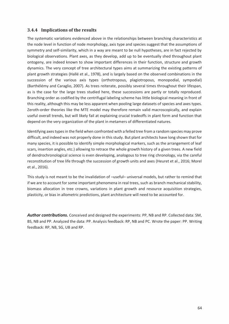
64
3.4.4 Implications of the results
The systematic variations evidenced above in the relationships between branching characteristics at
the node level in function of node morphology, axis type and species suggest that the assumptions of
symmetry and self-similarity, which in a way are meant to be null hypotheses, are in fact rejected by
biological observations. Plant axes, as they develop, add up to be eventually shed throughout plant
ontogeny, are indeed known to show important differences in their function, structure and growth
dynamics. The very concept of tree architectural types aims at summarizing the existing patterns of
plant growth strategies (Hallé et al., 1978), and is largely based on the observed combinations in the
succession of the various axis types (orthotropous, plagiotropous, monopodial, sympodial)
(Barthélémy and Caraglio, 2007). As trees reiterate, possibly several times throughout their lifespan,
as is the case for the large trees studied here, these successions are partly or totally reproduced.
Branching order as codified by the centrifugal labeling scheme has little biological meaning in front of
this reality, although this may be less apparent when pooling large datasets of species and axes types.
Zeroth-order theories like the MTE model may therefore remain valid macroscopically, and explain
useful overall trends, but will likely fail at explaining crucial tradeoffs in plant form and function that
depend on the very organization of the plant in metamers of differentiated natures.
Identifying axes types in the field when confronted with a felled tree from a random species may prove
difficult, and indeed was not properly done in this study. But plant architects have long shown that for
many species, it is possible to identify simple morphological markers, such as the arrangement of leaf
scars, insertion angles, etc.) allowing to retrace the whole growth history of a given trees. A new field
of dendrochronological science is even developing, analogous to tree ring chronology, via the careful
reconstitution of tree life through the succession of growth units and axes (Heuret et al., 2016; Morel
et al., 2016).
This study is not meant to be the invalidation of –useful– universal models, but rather to remind that
if we are to account for some important phenomena in real trees, such as branch mechanical stability,
biomass allocation in tree crowns, variations in plant growth and resource acquisition strategies,
plasticity, or bias in allometric predictions, plant architecture will need to be accounted for.
Author contributions. Conceived and designed the experiments: PP, NB and RP. Collected data: SM,
BS, NB and PP. Analyzed the data: PP. Analysis feedback: RP, NB and PC. Wrote the paper: PP. Writing
feedback: RP, NB, SG, UB and RP.
65
3.5. Reference
Aratsu, R., 1998. Leonardo was wise: trees conserve cross-sectional area despite vessel structure. J. Young Investig. 1, 1–20.
Barthélémy, D., Caraglio, Y., 2007. Plant Architecture: A Dynamic, Multilevel and Comprehensive Approach to Plant Form, Structure and Ontogeny. Ann. Bot. 99, 375–407. doi:10.1093/aob/mcl260
Bentley, L.P., Stegen, J.C., Savage, V.M., Smith, D.D., Allmen, E.I., Sperry, J.S., Reich, P.B., Enquist, B.J., 2013. An empirical assessment of tree branching networks and implications for plant allometric scaling models. Ecol. Lett. 16, 1069–1078.
Berninger, F., Nikinmaa, E., 1997. Implications of varying pipe model relationships on Scots pine growth in different climates. Funct. Ecol. 11, 146–156.
Bertram, J.A., 1989. Size-dependent differential scaling in branches: the mechanical design of trees revisited. Trees 3. doi:10.1007/BF00225358
Duursma, R.A., Mäkelä, A., Reid, D.E.B., Jokela, E.J., Porté, A.J., Roberts, S.D., 2010. Self-shading affects allometric scaling in trees: Self-shading and allometric scaling. Funct. Ecol. 24, 723–730. doi:10.1111/j.1365-2435.2010.01690.x
Eloy, C., 2011. Leonardo’s rule, self-similarity and wind-induced stresses in trees. Phys. Rev. Lett. 107, 258101. doi:10.1103/PhysRevLett.107.258101
Enquist, B.J., 2002. Universal scaling in tree and vascular plant allometry: toward a general quantitative theory linking plant form and function from cells to ecosystems. Tree Physiol. 22, 1045–1064. doi:10.1093/treephys/22.15-16.1045
Enquist, B.J., West, G.B., Brown, J.H., 2009. Extensions and evaluations of a general quantitative theory of forest structure and dynamics. Proc. Natl. Acad. Sci. 106, 7046–7051. doi:10.1073/pnas.0812303106
Greenhill, A.G., 1881. Determination of the greatest height consistent with stability that a vertical pole or mast can be made, and of the greatest height to which a tree of given proportions can grow. Proc. Camb. Philos. Soc.
Hallé, F., Oldeman, R.A.A., Tomlinson, P.B., 1978. Tropical trees and forests: an architectural analysis. Springer Verl. Berl. Heidelb. doi:10.1007/978-3-642-81190-6
Heuret, P., Caraglio, Y., Sabatier, S.-A., Barthélémy, D., Nicolini, E.-A., 2016. Retrospective analysis of plant architecture: an extended definition of dendrochronology.
Horn, H.S., 2000. Twigs, trees, and the dynamics of carbon in the landscape. Scaling Biol. 199–220. Horn, H.S., 1971. The adaptive geometry of trees. Princeton University Press. Kozlowski, J., Konarzewski, M., 2004. Is West, Brown and Enquist’s model of allometric scaling
mathematically correct and biologically relevant? Funct. Ecol. 18, 283–289. doi:10.1111/j.0269-8463.2004.00830.x
MacFarlane, D.W., Kuyah, S., Mulia, R., Dietz, J., Muthuri, C., Noordwijk, M.V., 2014. Evaluating a non-destructive method for calibrating tree biomass equations derived from tree branching architecture. Trees 1–11. doi:10.1007/s00468-014-0993-2
Mäkelä, A., 1986. Implications of the pipe model theory on dry matter partitioning and height growth in trees. J. Theor. Biol. 123, 103–120. doi:10.1016/S0022-5193(86)80238-7
McMahon, T.A., Kronauer, R.E., 1976. Tree structures: deducing the principle of mechanical design. J. Theor. Biol. 59, 443–466.
Minamino, R., Tateno, M., 2014. Tree Branching: Leonardo da Vinci’s Rule versus Biomechanical
Models. PLoS ONE 9, e93535. doi:10.1371/journal.pone.0093535 Morel, H., Mangenet, T., Heuret, P., Nicolini, E.-A., 2016. Studying phenology of tropical forest trees
using a morphological and anatomical retrospective analysis: the case of# Moronobea coccinea# Aubl.(Clusiaceae).
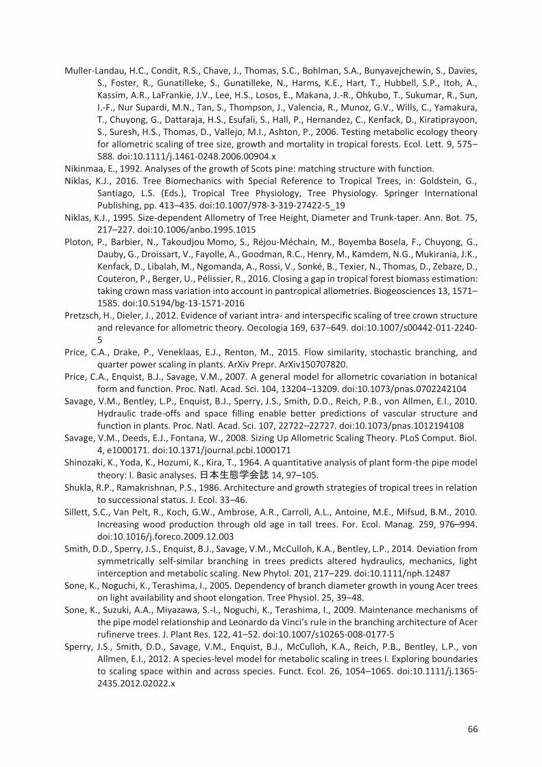
66
Muller-Landau, H.C., Condit, R.S., Chave, J., Thomas, S.C., Bohlman, S.A., Bunyavejchewin, S., Davies, S., Foster, R., Gunatilleke, S., Gunatilleke, N., Harms, K.E., Hart, T., Hubbell, S.P., Itoh, A., Kassim, A.R., LaFrankie, J.V., Lee, H.S., Losos, E., Makana, J.-R., Ohkubo, T., Sukumar, R., Sun, I.-F., Nur Supardi, M.N., Tan, S., Thompson, J., Valencia, R., Munoz, G.V., Wills, C., Yamakura, T., Chuyong, G., Dattaraja, H.S., Esufali, S., Hall, P., Hernandez, C., Kenfack, D., Kiratiprayoon, S., Suresh, H.S., Thomas, D., Vallejo, M.I., Ashton, P., 2006. Testing metabolic ecology theory for allometric scaling of tree size, growth and mortality in tropical forests. Ecol. Lett. 9, 575–
588. doi:10.1111/j.1461-0248.2006.00904.x Nikinmaa, E., 1992. Analyses of the growth of Scots pine: matching structure with function. Niklas, K.J., 2016. Tree Biomechanics with Special Reference to Tropical Trees, in: Goldstein, G.,
Santiago, L.S. (Eds.), Tropical Tree Physiology, Tree Physiology. Springer International Publishing, pp. 413–435. doi:10.1007/978-3-319-27422-5_19
Niklas, K.J., 1995. Size-dependent Allometry of Tree Height, Diameter and Trunk-taper. Ann. Bot. 75, 217–227. doi:10.1006/anbo.1995.1015
Ploton, P., Barbier, N., Takoudjou Momo, S., Réjou-Méchain, M., Boyemba Bosela, F., Chuyong, G., Dauby, G., Droissart, V., Fayolle, A., Goodman, R.C., Henry, M., Kamdem, N.G., Mukirania, J.K., Kenfack, D., Libalah, M., Ngomanda, A., Rossi, V., Sonké, B., Texier, N., Thomas, D., Zebaze, D., Couteron, P., Berger, U., Pélissier, R., 2016. Closing a gap in tropical forest biomass estimation: taking crown mass variation into account in pantropical allometries. Biogeosciences 13, 1571–
1585. doi:10.5194/bg-13-1571-2016 Pretzsch, H., Dieler, J., 2012. Evidence of variant intra- and interspecific scaling of tree crown structure
and relevance for allometric theory. Oecologia 169, 637–649. doi:10.1007/s00442-011-2240-5
Price, C.A., Drake, P., Veneklaas, E.J., Renton, M., 2015. Flow similarity, stochastic branching, and quarter power scaling in plants. ArXiv Prepr. ArXiv150707820.
Price, C.A., Enquist, B.J., Savage, V.M., 2007. A general model for allometric covariation in botanical form and function. Proc. Natl. Acad. Sci. 104, 13204–13209. doi:10.1073/pnas.0702242104
Savage, V.M., Bentley, L.P., Enquist, B.J., Sperry, J.S., Smith, D.D., Reich, P.B., von Allmen, E.I., 2010. Hydraulic trade-offs and space filling enable better predictions of vascular structure and function in plants. Proc. Natl. Acad. Sci. 107, 22722–22727. doi:10.1073/pnas.1012194108
Savage, V.M., Deeds, E.J., Fontana, W., 2008. Sizing Up Allometric Scaling Theory. PLoS Comput. Biol. 4, e1000171. doi:10.1371/journal.pcbi.1000171
Shinozaki, K., Yoda, K., Hozumi, K., Kira, T., 1964. A quantitative analysis of plant form-the pipe model theory: I. Basic analyses. 14, 97–105.
Shukla, R.P., Ramakrishnan, P.S., 1986. Architecture and growth strategies of tropical trees in relation to successional status. J. Ecol. 33–46.
Sillett, S.C., Van Pelt, R., Koch, G.W., Ambrose, A.R., Carroll, A.L., Antoine, M.E., Mifsud, B.M., 2010. Increasing wood production through old age in tall trees. For. Ecol. Manag. 259, 976–994. doi:10.1016/j.foreco.2009.12.003
Smith, D.D., Sperry, J.S., Enquist, B.J., Savage, V.M., McCulloh, K.A., Bentley, L.P., 2014. Deviation from symmetrically self-similar branching in trees predicts altered hydraulics, mechanics, light interception and metabolic scaling. New Phytol. 201, 217–229. doi:10.1111/nph.12487
Sone, K., Noguchi, K., Terashima, I., 2005. Dependency of branch diameter growth in young Acer trees on light availability and shoot elongation. Tree Physiol. 25, 39–48.
Sone, K., Suzuki, A.A., Miyazawa, S.-I., Noguchi, K., Terashima, I., 2009. Maintenance mechanisms of the pipe model relationship and Leonardo da Vinci’s rule in the branching architecture of Acer rufinerve trees. J. Plant Res. 122, 41–52. doi:10.1007/s10265-008-0177-5
Sperry, J.S., Smith, D.D., Savage, V.M., Enquist, B.J., McCulloh, K.A., Reich, P.B., Bentley, L.P., von Allmen, E.I., 2012. A species-level model for metabolic scaling in trees I. Exploring boundaries to scaling space within and across species. Funct. Ecol. 26, 1054–1065. doi:10.1111/j.1365-2435.2012.02022.x
67
Tredennick, A.T., Bentley, L.P., Hanan, N.P., 2013. Allometric Convergence in Savanna Trees and Implications for the Use of Plant Scaling Models in Variable Ecosystems. PLoS ONE 8, e58241. doi:10.1371/journal.pone.0058241
Tyree, M.T., 1988. A dynamic model for water flow in a single tree: evidence that models must account for hydraulic architecture. Tree Physiol. 4, 195–217.
von Allmen, E.I., Sperry, J.S., Smith, D.D., Savage, V.M., Enquist, B.J., Reich, P.B., Bentley, L.P., 2012. A species-level model for metabolic scaling of trees II. Testing in a ring- and diffuse-porous species. Funct. Ecol. 26, 1066–1076. doi:10.1111/j.1365-2435.2012.02021.x
West, G.B., Brown, J.H., Enquist, B.J., 1999. A general model for the structure and allometry of plant vascular systems. Nature 400, 664–667.
West, G.B., Brown, J.H., Enquist, B.J., 1997. A general model for the origin of allometric scaling laws in biology. Science 276, 122–126.
Yamamoto, K., Kobayashi, S., 1993. Analysis of crown structure based on the pipe model theory. Nippon Rin Gakkai-Shi 75, 445–448.
Zeide, B., 1998. Fractal analysis of foliage distribution in loblolly pine crowns. Can. J. For. Res. 28, 106–
114. doi:10.1139/cjfr-28-1-106 Zimmermann, M.H., 1978. Hydraulic architecture of some diffuse-porous trees. Can. J. Bot. 56, 2286–
2295.
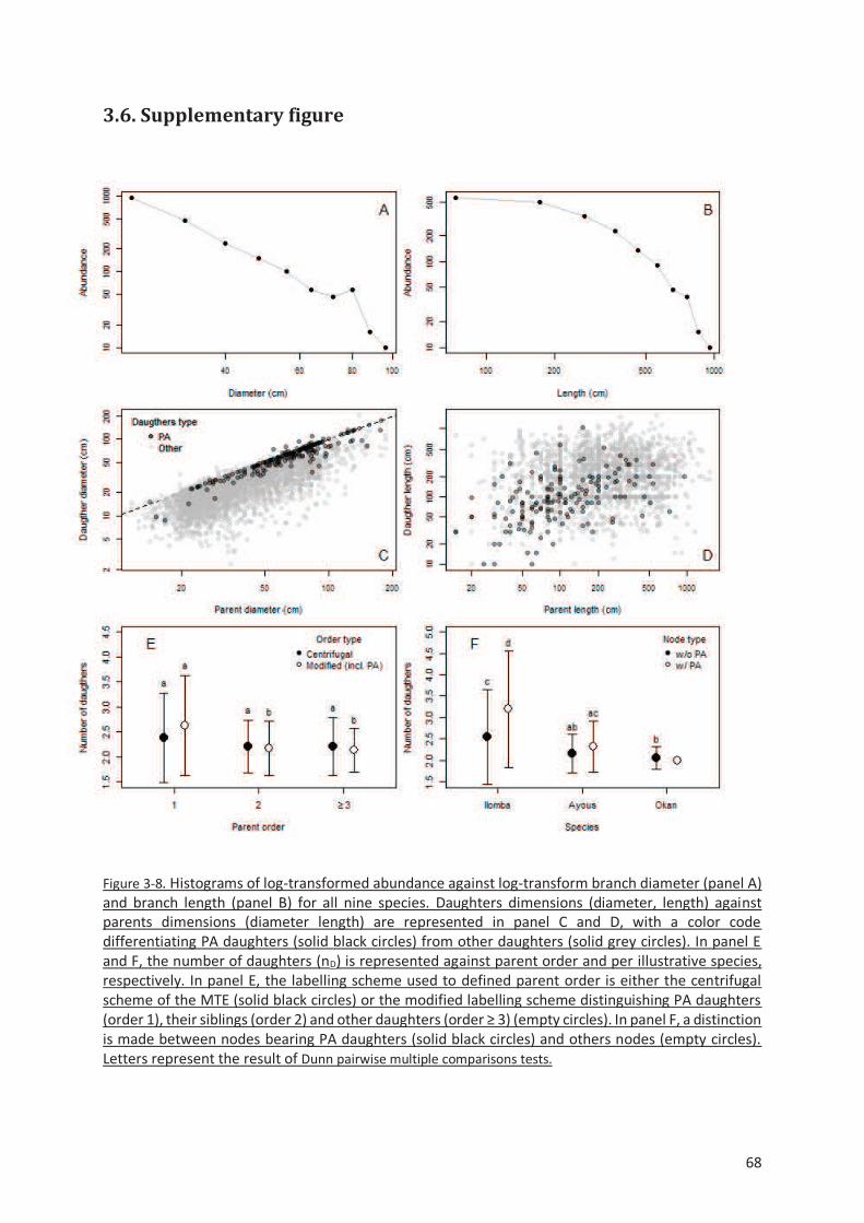
68
3.6. Supplementary figure
Figure 3-8. Histograms of log-transformed abundance against log-transform branch diameter (panel A) and branch length (panel B) for all nine species. Daughters dimensions (diameter, length) against parents dimensions (diameter length) are represented in panel C and D, with a color code differentiating PA daughters (solid black circles) from other daughters (solid grey circles). In panel E and F, the number of daughters (nD) is represented against parent order and per illustrative species, respectively. In panel E, the labelling scheme used to defined parent order is either the centrifugal scheme of the MTE (solid black circles) or the modified labelling scheme distinguishing PA daughters (order 1), their siblings (order 2) and other daughters (order ≥ 3) (empty circles). In panel F, a distinction
is made between nodes bearing PA daughters (solid black circles) and others nodes (empty circles). Letters represent the result of Dunn pairwise multiple comparisons tests.
69
4 CANOPY TEXTURE ANALYSIS FOR LARGE-SCALE
ASSESSMENTS OF TROPICAL FOREST STAND
STRUCTURE AND BIOMASS
P. Ploton1,2, R. Pélissier1,3, N. Barbier2, C. Proisy3, B.R. Ramesh1 & P. Couteron3.
1Ecology Department, French Institute of Pondicherry, UMIFRE 21 MAEE-CNRS, Pondicherry 605001, India 2IRD, UMR AMAP, University of Yaounde I, Yaounde, Cameroon 3IRD, UMR AMAP, F- 34000 Montpellier, France
Abstract
The structural organization of a forest canopy is an important descriptor that may provide information
for vegetation mapping and management planning. We present a new approach of canopy texture
analysis from diverse very-high remotely sensed optical image types, such as digitized aerial
photographs, very-high resolution satellite scenes or Google Earth extractions. Based on the
multivariate ordination of Fourier spectra, the FOTO method allows us to ordinate canopy images with
respect to canopy grain, i.e. a combination of mean size and density of tree crowns per sampling
window. Confronted to field data in different contexts across the tropics, in mangroves, evergreen to
semi-evergreen lowland and mountain forests, FOTO-derived indices proved powerful for consistently
retrieving certain stand structure parameters, notably aboveground biomass up to the highest levels
observed. We illustrate the potential of the texture-structure model inversion for predicting stand
structure parameters over vast poorly documented forest areas in India, Amazonia and central Africa.
We lastly draw research perspectives to overcome current limits of the method, such as instrumental
and topography-induced biases.
70
4.1 Introduction
The structural organization of a forest canopy is an important descriptor that may provide spatial
information for vegetation mapping and management planning, such as attributes of plant species
distributions, intensity of disturbances, aboveground biomass or carbon stock. A variety of airborne
and satellite images have long been used to characterize forest stands from above the canopy,
providing the advantage of a rapid exploration of extensive and sometimes difficultly accessible zones.
Unfortunately this approach proved to be of limited applicability in wet tropical regions, notably
because most optical and radar signals that deliver medium to high spatial resolution data have shown
to saturate at intermediate levels of biomass ranges (ca. 150-200 Mg.ha-1) or leaf area index values
(Gibbs et al., 2007). As a consequence, while forest vs. non-forest classifications are nowadays
routinely performed from such data, variations in stand structure and biomass within forests of fairly
closed canopy remain almost undetectable with classical techniques and the forest treetops seen from
above appear generally as a homogeneously undulating green carpet. There is however a lot of
ecological evidence that rainforest structure substantially varies from place to place either naturally
(as the soil, composition or forest dynamics vary) or resulting from anthropogenic degradations.
Detecting, characterizing and mapping these variations over vast areas become particularly challenging
within the perspective of the REDD+ agenda (Maniatis and Mollicone, 2010), which requests
participating countries to periodically monitor their carbon stock variation. While promising
developing instruments such as LiDAR (Light Detection and Ranging) are potentially powerful in this
perspective, they remain very expensive to systematically operate for large-scale forest assessments
in the tropics (but see Asner et al., 2010). We recently developed as a cost-effective alternative, a
method of canopy grain texture analysis from very-high resolution air- or space-borne images, which
proved efficient for retrieving and mapping stand structure parameters including abovegound biomass
over vast poorly documented areas of tropical forest.
4.2 Methodological background and rationale
Given allometric relationships that exist between individual tree dimensions (such as trunk diameter,
height and crown size), our approach stems from the idea that the number and size of tree crowns
visible from above the canopy should inform on some other forest structural parameters. The
reasoning is straightforward when considering for instance stand basal area (G) or aboveground
biomass (AGB) in closed forest conditions since in this case the largest trees that reach the canopy can
account for up to 70-80% of stand level values. However the renewed interest for allometric scaling in
ecology (Enquist et al., 2009), suggests that tree dimensions and their size frequency distribution, may
be relevant to infer stand properties, such as spacing relations, mortality rates or stand dynamics, from
canopy characteristics. While most previous attempts were based on visual or automated delineations
of individual tree crowns from very-high resolution (VHR) canopy images, we present hereafter a more
holistic characterization of canopy geometrical properties through canopy grain texture analysis by
two-dimensional Fourier power spectrum. The main outlines of the method that we named FOurier
Textural Ordination (FOTO) are illustrated in Figure 4-1. From a digital VHR panchromatic canopy
image, optionally masked for non-forested areas (clouds, water bodies, bare soils, etc.), a set of square
windows with size set to include several repetitions of the largest textural pattern that compose
canopy grain is first extracted (Figure 4-1 a). For closed-canopy scenes, canopy grain results from the
shape, size and spatial arrangement of dominant tree crowns, so that square windows of about 1 ha
proved to be a good option. A Fourier radial power spectrum (or r-spectrum) is then computed for

71
each window, which features how image grey levels' variance partitions into increasing spatial
frequency bins (in cycles.km-1 i.e. the number of repetitions over 1 km) or equivalently into
wavelengths (pattern sizes in m) (see Couteron, 2002 for further details). In other words, a r-spectrum
represents the frequency distribution of pattern sizes in the canopy grain: while coarse canopy grain
yields r-spectra significantly skewed towards small frequencies (large wavelengths), fine canopy grain
yields r-spectra significantly skewed towards large frequencies (small wavelengths;Figure 4-1 b). All
windows' r-spectra computed from a VHR canopy image can then be stacked into a single matrix with
the canopy windows (observations) as rows and the spatial frequencies (variables) as columns (Figure
4-1 c). Such a matrix may be submitted to a standardized-PCA that systematically compares the canopy
windows with respect to the relative importance of spatial frequencies in their respective spectra. The
typical clockwise distribution of the spatial frequency variables in the first PCA plane straightforwardly
creates a canopy texture gradient which ordinates canopy windows, from coarse- to fine-grained
patterns (Figure 4-1 d). Windows' scores against the main PCA axes thus represent canopy texture
indices (so-called FOTO indices), which can be related to control plots data using multivariate linear
models, to calibrate and assess the indices’ ability to infer stand structure parameters (Figure 4-1 e).
Once calibrated, texture-structure relationships can be inverted for predicting and mapping stand
structure parameters over the whole area covered by the initial VHR image (Figure 4-1 f).
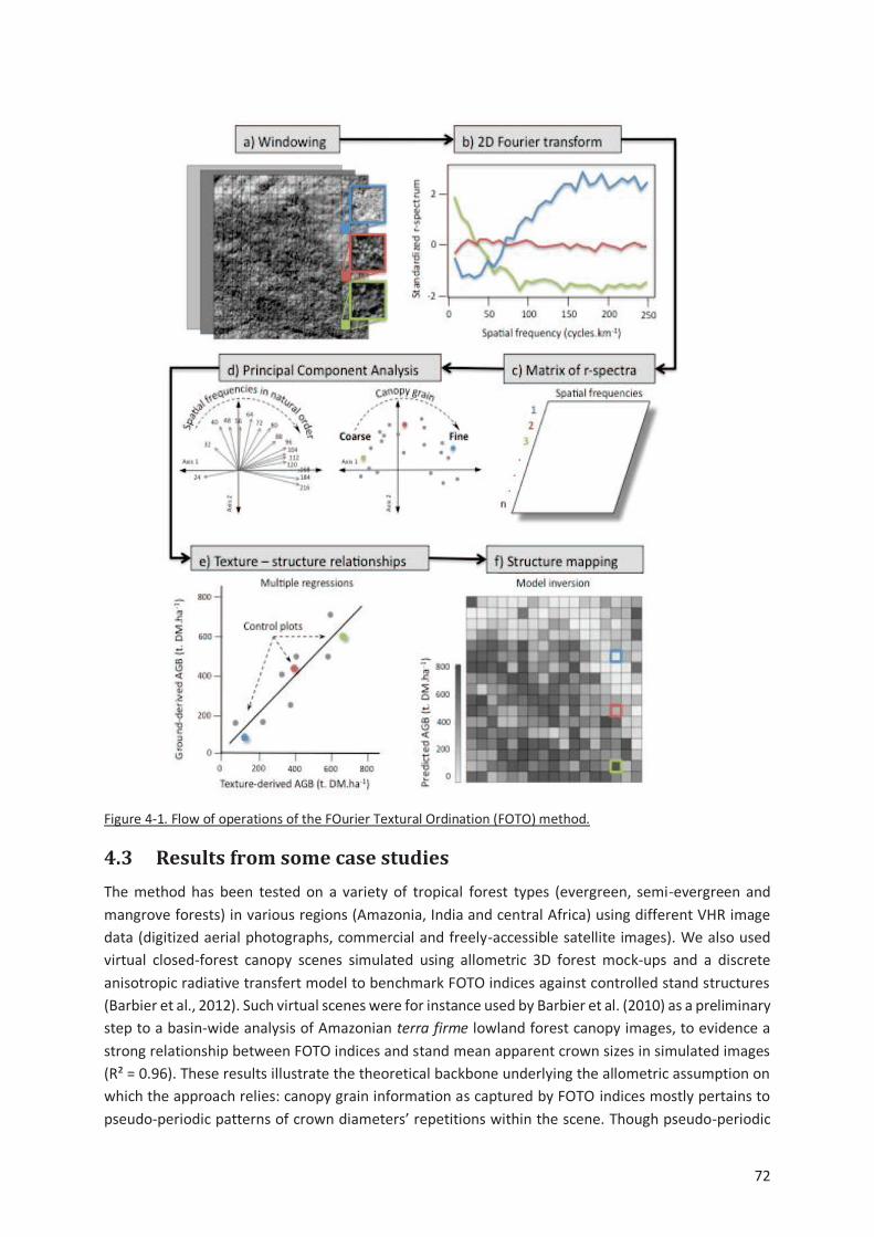
72
Figure 4-1. Flow of operations of the FOurier Textural Ordination (FOTO) method.
4.3 Results from some case studies
The method has been tested on a variety of tropical forest types (evergreen, semi-evergreen and
mangrove forests) in various regions (Amazonia, India and central Africa) using different VHR image
data (digitized aerial photographs, commercial and freely-accessible satellite images). We also used
virtual closed-forest canopy scenes simulated using allometric 3D forest mock-ups and a discrete
anisotropic radiative transfert model to benchmark FOTO indices against controlled stand structures
(Barbier et al., 2012). Such virtual scenes were for instance used by Barbier et al. (2010) as a preliminary
step to a basin-wide analysis of Amazonian terra firme lowland forest canopy images, to evidence a
strong relationship between FOTO indices and stand mean apparent crown sizes in simulated images
(R² = 0.96). These results illustrate the theoretical backbone underlying the allometric assumption on
which the approach relies: canopy grain information as captured by FOTO indices mostly pertains to
pseudo-periodic patterns of crown diameters’ repetitions within the scene. Though pseudo-periodic
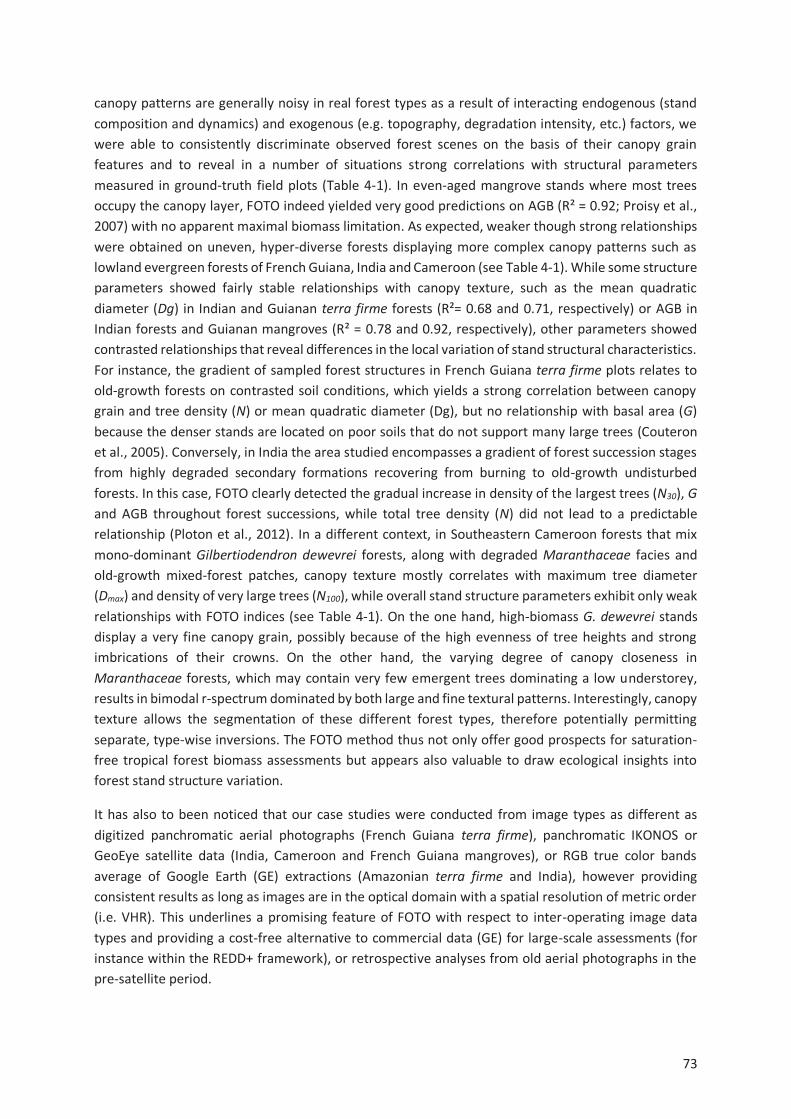
73
canopy patterns are generally noisy in real forest types as a result of interacting endogenous (stand
composition and dynamics) and exogenous (e.g. topography, degradation intensity, etc.) factors, we
were able to consistently discriminate observed forest scenes on the basis of their canopy grain
features and to reveal in a number of situations strong correlations with structural parameters
measured in ground-truth field plots (Table 4-1). In even-aged mangrove stands where most trees
occupy the canopy layer, FOTO indeed yielded very good predictions on AGB (R² = 0.92; Proisy et al.,
2007) with no apparent maximal biomass limitation. As expected, weaker though strong relationships
were obtained on uneven, hyper-diverse forests displaying more complex canopy patterns such as
lowland evergreen forests of French Guiana, India and Cameroon (see Table 4-1). While some structure
parameters showed fairly stable relationships with canopy texture, such as the mean quadratic
diameter (Dg) in Indian and Guianan terra firme forests (R²= 0.68 and 0.71, respectively) or AGB in
Indian forests and Guianan mangroves (R² = 0.78 and 0.92, respectively), other parameters showed
contrasted relationships that reveal differences in the local variation of stand structural characteristics.
For instance, the gradient of sampled forest structures in French Guiana terra firme plots relates to
old-growth forests on contrasted soil conditions, which yields a strong correlation between canopy
grain and tree density (N) or mean quadratic diameter (Dg), but no relationship with basal area (G)
because the denser stands are located on poor soils that do not support many large trees (Couteron
et al., 2005). Conversely, in India the area studied encompasses a gradient of forest succession stages
from highly degraded secondary formations recovering from burning to old-growth undisturbed
forests. In this case, FOTO clearly detected the gradual increase in density of the largest trees (N30), G
and AGB throughout forest successions, while total tree density (N) did not lead to a predictable
relationship (Ploton et al., 2012). In a different context, in Southeastern Cameroon forests that mix
mono-dominant Gilbertiodendron dewevrei forests, along with degraded Maranthaceae facies and
old-growth mixed-forest patches, canopy texture mostly correlates with maximum tree diameter
(Dmax) and density of very large trees (N100), while overall stand structure parameters exhibit only weak
relationships with FOTO indices (see Table 4-1). On the one hand, high-biomass G. dewevrei stands
display a very fine canopy grain, possibly because of the high evenness of tree heights and strong
imbrications of their crowns. On the other hand, the varying degree of canopy closeness in
Maranthaceae forests, which may contain very few emergent trees dominating a low understorey,
results in bimodal r-spectrum dominated by both large and fine textural patterns. Interestingly, canopy
texture allows the segmentation of these different forest types, therefore potentially permitting
separate, type-wise inversions. The FOTO method thus not only offer good prospects for saturation-
free tropical forest biomass assessments but appears also valuable to draw ecological insights into
forest stand structure variation.
It has also to been noticed that our case studies were conducted from image types as different as
digitized panchromatic aerial photographs (French Guiana terra firme), panchromatic IKONOS or
GeoEye satellite data (India, Cameroon and French Guiana mangroves), or RGB true color bands
average of Google Earth (GE) extractions (Amazonian terra firme and India), however providing
consistent results as long as images are in the optical domain with a spatial resolution of metric order
(i.e. VHR). This underlines a promising feature of FOTO with respect to inter-operating image data
types and providing a cost-free alternative to commercial data (GE) for large-scale assessments (for
instance within the REDD+ framework), or retrospective analyses from old aerial photographs in the
pre-satellite period.
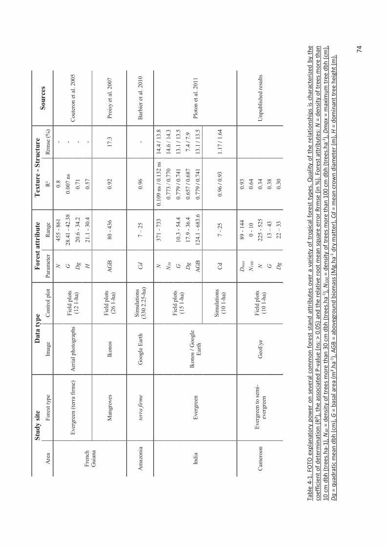
74
Tab
le 4
-1.
FOTO
exp
lan
ato
ry p
ow
er o
n s
ever
al c
om
mo
n fo
rest
sta
nd
att
rib
utes
ove
r a
vari
ety
of
tro
pic
al f
ore
st t
ypes
. Q
ual
ity
of
the
rela
tio
nsh
ips
is c
har
acte
rize
d b
y th
e co
effi
cien
t o
f d
eter
min
atio
n (
R²)
, th
e as
soci
ated
P-v
alu
e (n
s: >
0.0
5) a
nd
the
rel
ativ
e ro
ot
mea
n s
qu
are
erro
r R
rmse
(in
%).
Fo
rest
att
rib
ute
s: N
= d
ensi
ty o
f tr
ees
mo
re t
han
10
cm
dbh
(tr
ees.
ha-
1), N
30 =
den
sity
of
tree
s m
ore
th
an 3
0 cm
db
h (t
rees
.ha-1
), N
10
0 =
den
sity
of
tree
s m
ore
th
an 1
00 c
m d
bh
(tr
ees.
ha-1
), D
ma
x =
max
imum
tre
e d
bh
(cm
),
Dg
= q
uad
rati
c m
ean
db
h (
cm),
G =
bas
al a
rea
(m².
ha-1
), A
GB
= a
bo
vegr
ou
nd
bio
mas
s (M
g.h
a-1 d
ry m
atte
r), C
d =
mea
n cr
ow
n d
iam
eter
(m
), H
= d
omin
ant
tree
hei
ght
(m).
Stu
dy s
ite
Data
typ
e
Fores
t att
rib
ute
T
extu
re -
Str
uctu
re
S
ou
rce
s A
rea
Fore
st t
ype
Imag
e
Con
trol
plo
t P
aram
eter
R
ange
R²
Rrm
se (
%)
Fre
nch
G
uia
na
Ever
gre
en (
terr
a fi
rme)
A
eria
l p
hoto
gra
phs
Fie
ld p
lots
(1
2 1
-ha)
N
45
5 -
86
1
0.8
-
Cou
tero
n e
t al
. 2
00
5
G
28
.41
- 4
2.3
8
0.0
07
ns
-
Dg
2
0.6
- 3
4.2
0
.71
-
H
21
.1 -
30
.4
0.5
7
-
Man
gro
ves
Ik
on
os
Fie
ld p
lots
(26 1
-ha)
A
GB
8
0 -
43
6
0.9
2
17
.3
Pro
isy
et a
l. 2
007
Am
azo
nia
te
rra f
irm
e G
oogle
Ear
th
Sim
ula
tion
s
(33
0 2
.25
-ha)
C
d
7 –
25
0.9
6
- B
arbie
r et
al.
201
0
Ind
ia
Ever
gre
en
Ikon
os
/ G
oo
gle
E
arth
Fie
ld p
lots
(1
5 1
-ha)
N
37
1 -
73
3
0.1
09
ns
/ 0.1
32 n
s 1
4.4
/ 1
3.8
Plo
ton
et
al. 2
01
1
N3
0
0
.773
/ 0
.77
0
14
.6 /
14
.3
G
10
.3 -
54
.4
0.7
79
/ 0
.74
1
13
.1 /
13
.5
Dg
1
7.9
- 3
6.4
0
.657
/ 0
.68
7
7.4
/ 7
.9
AG
B
12
4.1
- 6
83.6
0
.779
/ 0
.74
1
13
.1 /
13
.5
Sim
ula
tion
s
(10 1
-ha)
C
d
7 -
25
0.9
6 /
0.9
3
1.1
7 /
1.6
4
Cam
eroon
E
ver
gre
en t
o s
emi-
ever
gre
en
Geo
Eye
F
ield
plo
ts
(10 1
-ha)
Dm
ax
89
- 1
44
0.9
3
N1
00
0 -
10
0.6
4
N
22
5 -
52
5
0.3
4
U
np
ubli
shed
res
ult
s
G
13
– 4
3
0.3
8
Dg
2
2 –
33
0.3
0
75
4.4 Limits and perspectives
Further case studies and simulation works are going on to validate the FOTO method in various tropical
forest contexts. One of the limits of the canopy grain approach arises when canopy texture properties
deviate too much from a pseudo-periodicity so that the main canopy pattern does not result from
repetitions of crown diameters. Such heterogeneity may result from the presence of canopy gaps or
treefalls of varying sizes, or of contrasted illumination patterns due to abrupt relief variations (e.g. two
sides of a ridge line or a deep thalweg). Typically, r-spectra of windows displaying a high degree of
spatial heterogeneity are skewed towards low frequencies due to the contribution of heterogeneity to
the largest size patterns. It follows that such windows can be erroneously interpreted as containing
large tree crowns and must be removed from the analysis so not to bias the texture-structure
relationship (Ploton et al., 2012). Similarly, when shifting from pure evergreen to semi-evergreen or
mixed deciduous tropical forest types, textural information may be influenced by seasonal changes in
the canopy that still require to be investigated.
Though the FOTO method offers good prospects for large-scale implementation, further difficulties
arise when several canopy images with different acquisition parameters have to be mosaicked. Indeed,
the sun-scene-sensor geometry influences the size and proportion of tree shadows in the canopy
scene, and thus modifies the textural properties as detected by Fourier r-spectrum. To ensure a
consistent comparison between different canopy scenes, one must either use images with similar
acquisition conditions, or correct for the influences of changing acquisition conditions on canopy
textural properties. To this end, Barbier et al. (2011) introduced a Bidirectional Texture Function (BTF)
that allows correcting for instrumental bias based on a partitioned standardization of the r-spectrum
prior to PCA. A very similar problem arises with relief variations, which modify the proportion of sun-
lighted vs. shadowed crowns. In mountainous regions, this effect has the potential to make FOTO
detecting a finer grain on illuminated hillsides and coarser grain on shaded ones regardless of forest
structure. A partitioned standardization of the r-spectrum according to hillshade classes may also
provide a solution to correct for such a bias (Ploton, 2010).
Author contributions. Wrote the paper: PP. Writing feedback: RP, NB, CP, BRR and PC.
76
4.5 Reference
Asner, G.P., Powell, G.V.N., Mascaro, J., Knapp, D.E., Clark, J.K., Jacobson, J., Kennedy-Bowdoin, T.,
Balaji, A., Paez-Acosta, G., Victoria, E., Secada, L., Valqui, M., Hughes, R.F., 2010. High-resolution forest
carbon stocks and emissions in the Amazon. Proc. Natl. Acad. Sci. 107, 16738–16742.
doi:10.1073/pnas.1004875107
Barbier, N., Couteron, P., Gastelly-Etchegorry, J.-P., Proisy, C., 2012. Linking canopy images to forest
structural parameters: potential of a modeling framework. Ann. For. Sci. 69, 305–311.
doi:10.1007/s13595-011-0116-9
Barbier, N., Couteron, P., Proisy, C., Malhi, Y., Gastellu-Etchegorry, J.-P., 2010. The variation of
apparent crown size and canopy heterogeneity across lowland Amazonian forests. Glob. Ecol.
Biogeogr. 19, 72–84.
Barbier, N., Proisy, C., Véga, C., Sabatier, D., Couteron, P., 2011. Bidirectional texture function of high
resolution optical images of tropical forest: An approach using LiDAR hillshade simulations. Remote
Sens. Environ. 115, 167–179.
Couteron, P., 2002. Quantifying change in patterned semi-arid vegetation by Fourier analysis of
digitized aerial photographs. Int. J. Remote Sens. 23, 3407–3425.
Couteron, P., Pelissier, R., Nicolini, E.A., Paget, D., 2005. Predicting tropical forest stand structure
parameters from Fourier transform of very high-resolution remotely sensed canopy images. J. Appl.
Ecol. 42, 1121–1128.
Enquist, B.J., West, G.B., Brown, J.H., 2009. Extensions and evaluations of a general quantitative theory
of forest structure and dynamics. Proc. Natl. Acad. Sci. 106, 7046–7051. doi:10.1073/pnas.0812303106
Gibbs, H.K., Brown, S., Niles, J.O., Foley, J.A., 2007. Monitoring and estimating tropical forest carbon
stocks: making REDD a reality. Environ. Res. Lett. 2, 045023.
Maniatis, D., Mollicone, D., 2010. Options for sampling and stratification for national forest inventories
to implement REDD+ under the UNFCCC. Carbon Balance Manag. 5, 1.
Ploton, P., 2010. Analyzing canopy heterogeneity of the tropical forests by texture analysis of very-high
resolution images-A case study in the Western Ghats of India.
Ploton, P., Pélissier, R., Proisy, C., Flavenot, T., Barbier, N., Rai, S.N., Couteron, P., 2012. Assessing
aboveground tropical forest biomass using Google Earth canopy images. Ecol. Appl. 22, 993–1003.
doi:10.1890/11-1606.1
Proisy, C., Couteron, P., Fromard, F., 2007. Predicting and mapping mangrove biomass from canopy
grain analysis using Fourier-based textural ordination of IKONOS images. Remote Sens. Environ. 109,
379–392.
77
5 TOWARD A GENERAL TROPICAL FOREST BIOMASS
PREDICTION MODEL FROM VERY HIGH RESOLUTION
OPTICAL SATELLITE IMAGES
P. Ploton1,2, N. Barbier1, P. Couteron1, C.M. Antin1, N. Ayyappan3, N. Balachandran3, N. Barathan3, J.-F. Bastin4, G. Chuyong5, G. Dauby6,7, V. Droissart1,8, J.-P. Gastellu-Etchegorry9, N.G. Kamdem10, D.
Kenfack11, M. Libalah10, G.II. Mofack10, S.T. Momo1, 10, S. Pargal1, P. Petronelli12, C. Proisy1,3, M. Réjou-Méchain1,3, B. Sonké10, N. Texier1, 10, D. Thomas13, P. Verley1, D. Zebaze Dongmo10, U. Berger14 and R.
Pélissier1,3
1Institut de Recherche pour le Développement, UMR-AMAP, Montpellier, France 2Institut des sciences et industries du vivant et de l'environnement, Montpellier, France 3French Institute of Pondicherry, Puducherry, India 4Landscape Ecology and Plant Production Systems Unit, Université Libre de Bruxelles, Brussels, Belgium 5Department of Botany and Plant Physiology, University of Buea, Buea, Cameroon 6Institut de Recherche pour le Développement, UMR-DIADE, Montpellier, France 7Evolutionary Biology and Ecology, Faculté des Sciences, Université Libre de Bruxelles, Brussels, Belgium 8Herbarium et Bibliothèque de Botanique africaine, Université Libre de Bruxelles, Brussels, Belgium 9Université Paul Sabatier, CESBIO, Toulouse, France 10Laboratoire de Botanique systématique et d'Ecologie, Département des Sciences Biologiques, Ecole Normale Supérieure, Université de Yaoundé I, Yaoundé, Cameroon 11Center for Tropical Forest Science — Forest Global Earth observatory, Smithsonian Tropical Research Institute, Washington, USA 12Centre de coopération Internationale en Recherche Agronomique pour le Développement, UMR-ECOFOG, Kourou, France 13Department of Biological Sciences, Washington State University, Vancouver, U.S.A. 14Technische Universität Dresden, Faculty of Environmental Sciences, Institute of Forest Growth and Forest Computer Sciences, Tharandt, Germany
ABSTRACT
Very high spatial resolution (VHSR) optical data have shown a good potential to provide non-saturating
proxies of tropical forest aboveground biomass (AGB), notably from canopy texture features extracted
with Fourier transform. However, the relationships between Fourier texture features and forest AGB
varies among forest types and regions of the world, hampering the deployment of a broad scale forest
carbon monitoring method based on these sole texture metrics. Our aim here was to complement
Fourier texture features with additional information on forest structure to generalize the texture-
based approach. We explored how canopy texture properties related to forest AGB estimation using
279 1-ha tropical forest inventory plots distributed across the tropics for which we simulated VHSR
optical canopy scenes. This allowed controlling for instrumental effects and focusing on the sole
canopy texture features – forest AGB relations. Globally, Fourier texture of simulated canopies
significantly explained AGB variations (R²=0.46), with an uncertainty of c. 30%. The strength of this
relationship varied among sites with higher accuracy found on forests with close, fairly periodic
78
canopies (reflecting a self-thinning process) while heterogeneity in stand and canopy structure
(reflecting gap phase dynamics) was detrimental. We found that including a gradient of canopy
heterogeneity from a lacunarity analysis largely improved AGB model performances (R²=0.76,
rRMSE=20%). As texture analysis of two-dimensional images cannot retrieve large-scale variations in
forest height, a bioclimatic proxy of tree slenderness further improved model goodness-of-fit at the
global level (R²=0.88) and reduced model error at the local level (reduction of site-level prediction
biases). The final texture-based approach was tested on a set of 3 Pleiades images covering a complex
mosaic of forest types in the Congo basin and led to uncertainty levels (RMSE = 62 Mg.ha-1,
rRMSE=21%) comparable to those obtained from airborne LiDAR-based models. The increasing
availability of VHSR optical sensors (such as from constellations of small satellite platforms) raises the
possibility of routine repeated imaging of the world’s tropical forests and suggests that texture-based
analyses could become an essential tool in international efforts to monitor carbon emissions from
deforestation and forest degradations (REDD+ program).
5.1 Introduction
Concerns about the effects of increasing atmospheric carbon on climate have led to an international
program aiming at reducing emissions of greenhouse gases from deforestation and forest
degradations (UN-REDD+ program), notably in the tropics where the bulk of global deforestation
occurs (Pan et al., 2011). REDD+ implementation fundamentally relies on our capacity to monitor forest
carbon stock and dynamics at multiple spatial scales, from entire countries down to scales at which
deforestation and degradation processes occur. In this context, remote sensing naturally becomes an
essential tool (Baccini et al., 2012; DeFries et al., 2007; Saatchi et al., 2011). However, remote sensing
of forest carbon stocks (often through forest aboveground biomass, hereafter denoted AGB) is
challenging in the tropics because most satellite sensors are not sensitive to AGB variation above c.
150 Mg.ha-1, while tropical forests AGB often exceeds 400 Mg.ha-1 (Slik et al., 2013). This saturation is
well documented for passive optical sensors of coarse to intermediate spatial resolution such as the
Moderate Resolution Imaging Spectroradiometer (MODIS) or Landsat Thematic Mapper (e.g. Lu, 2006;
Lu et al., 2012; Zhao et al., 2016) but also for radar signals (notably L-band SAR, Mermoz et al., 2015),
and thus constitutes a crippling limit for those data types. Aircraft-based light detection and ranging
(A-LiDAR) systems have become vastly popular for about a decade in tropical forest studies, as they
appear to be free of saturation. Small-footprint A-LiDAR data provide a detailed description of forest
three-dimensional (3D) structure from which forest AGB can be estimated with reasonable confidence
(c. 15% relative error on 1-ha plots, e.g. Réjou-Méchain et al., 2015; Zolkos et al., 2013). Unfortunately
this information comes at a cost rendering the wall-to-wall and regular coverage of large territories
uneconomical (Erdody and Moskal, 2010; Messinger et al., 2016). A potentially interesting alternative
to A-LiDAR for large-scale monitoring of tropical forests may be found in very high spatial resolution
(VHSR) optical images, as they are routinely captured by a range of satellite platforms and, therefore,
does not involve costly airborne data acquisition campaigns. The improvement brought by the
increased spatial resolution over coarser, widely-used optical data (e.g. Landsat), lies on a fundamental
change in the analysis: at metric to sub-metric resolutions, individual trees are now discernable in the
image, allowing one to exploit the geometric properties of tree crowns (i.e. crown delineation
algorithms, e.g. Broadbent et al., 2008; Zhou et al., 2013) or forest canopies (i.e. texture analysis, e.g.
79
Couteron et al., 2005) that conceptually more directly relate to stand biomass than spectral greenness
indices.
Texture analysis of panchromatic VHSR canopy images (e.g. Couteron et al., 2005; Frazer et al., 2005)
have shown promising results to retrieve stand and canopy forest attributes, including tropical forest
AGB with no sign of saturation (e.g. Bastin et al., 2014; Ploton et al., 2012). Generally speaking, texture
analysis (sensu Haralick, 1979) gives us a measure of the spatial arrangement of grey levels within a
canopy image by directly reflecting the contrasts between sunlit and shadowed surfaces, thus
providing information on the size and distribution of crowns of canopy trees and inter-crowns canopy
gaps. Texture is scale-dependent, so that meaningful texture metrics have to be multi-scale by nature
(e.g. Fourier r-spectra; Couteron, 2002) or measurable at multiple scales (e.g. lacunarity; Frazer et al.,
2005). Those analyses are often carried out on image excerpts over scales related to local variations in
crown and gap sizes (e.g. canopy window of c. 1-ha) while comparing texture features, whatever their
source, over very large forest tracts (e.g. hundreds of square kilometers). A systematic comparison
between canopy windows texture features can be performed through standard multivariate
ordination technics (e.g. Principal Component Analysis). Principal axes thus display canopy windows
along uncorrelated texture and spatial heterogeneity gradients that facilitate their separation and
interpretation. Window scores on the principal axes are then used as dependent variables (texture
indices) in regression analyses in order to examine the statistical relationship between canopy texture
and stand structure parameters, for instance AGB, as measured from field plots data (e.g. Couteron et
al., 2005; Proisy et al., 2007). The basic idea is that once calibrated such relationships can be inverted
to predict and map stand structure parameters outside the sampling plots from texture analysis of
VHSR panchromatic images.
To date, the FOurier Textural Ordination (or FOTO method; Couteron, 2002; Proisy et al., 2007) has
been applied in a number of tropical forest case studies to derive plot-level AGB estimates from
panchromatic canopy images (e.g. Ploton et al., 2012; Proisy et al., 2007; Singh et al., 2014) or LiDAR
Canopy Height Models (e.g. Véga et al., 2015). Study footprint is generally a few hundreds of square
kilometers covered by one or two VHSR images. At this scale, the texture gradient provides good
relationships with forest stand structure parameters, with a relative error on 1-ha plot AGB
estimations, generally below 20%. It has indeed been demonstrated from simulations that in closed-
forest canopies, FOTO-texture indices characterize the size distribution of canopy crowns (Barbier et
al., 2012), which are allometrically linked to tree size and AGB (Jucker et al., 2016; Ploton et al., 2016).
It is increasingly evident, however, that the texture-structure relationship is forest type- and/or site-
dependent (Bastin et al., 2014), thus limiting broad-scale applications. As a consequence, texture
analysis of large mixed-forest landscapes currently requires a stratification into homogeneous texture-
AGB strata as in the forest mosaics of the Congo basin (Bastin et al., 2014). It is worth mentioning that
similar limitations have been encountered for LiDAR-based studies, requiring complementary
information layers to allow multi-site comparisons (e.g. Asner et al., 2011; Vincent et al., 2014, 2012).
Generalizing the texture-structure relationship across contrasted forest types from different regions
of the world would therefore be a major step towards an operational method to monitor forest
structure and AGB from VHSR optical data.
Here, our hypothesis is that canopy heterogeneity created by different environmental conditions and
canopy gap dynamics may influence the texture-structure relationship derived from the FOTO method.
In a VHSR canopy image, tree crowns and gaps are visible to the naked-eye from local brightness
80
variations, but texture patterns captured by FOTO cannot discriminate large tree crowns from canopy
gaps as they both appear as aggregates of bright or dark pixels of similar size in the image. Coarse
texture thus indistinctively results from closed canopies comprised of large tree crowns and from open
canopies where aggregates of tree crowns alternate with canopy openings. Thus, a same texture may
represent high or low AGB values, respectively. To overcome this drawback, FOTO texture can be
complemented by other textural features characterizing canopy heterogeneity at multiple scales, such
as lacunarity, which proved to correlate well with canopy cover and gap volume on simulated forest
stands (Frazer et al., 2005).
Another constraint limiting the empirical exploration of the link between canopy texture and the
underlying forest stand structure over large regions covered by several VHSR images is of instrumental
nature. Forest texture indices are indeed sensitive to sensor optical properties and spatial resolution
(Ploton et al., 2012; Proisy et al., 2007), but also to sun-sensor geometry (Barbier et al., 2011; Barbier
and Couteron, 2015). Disentangling the effect of forest structure on canopy texture from instrumental
effects thus requires having a sufficiently large set of VHSR images acquired in homogeneous sun-
sensor configurations and covering an extensive field plot network. An efficient workaround is to adopt
a modelling approach coupling the simulation of 3D forest stand mockups and the generation of virtual
canopy images by applying a radiative transfer model onto the 3D mockups (Barbier et al., 2012). By
controlling parameters of the radiative transfer model, canopy images in identical acquisition
configurations can be generated for a variety of 3D stand mockups. Forest mockups built from simple
tree shapes derived from field data (tree location, height, diameter and crown dimensions) allow
bridging the gap between ground observations and remote sensing data (e.g. Frazer et al. 2005,
Schneider et al., 2014). They ultimately help us to translate signal information into biophysical
parameters. Modeling trees with simple geometrical shapes and homogeneous optical properties may
appear as a coarse representation of reality, but it led to valuable insights into how the 3D arrangement
of stems and leaves is linked to important processes of the forest dynamics (Stark et al., 2015; Taubert
et al., 2015).
In this study, we compiled data from 279 1-ha forest inventory plots from several tropical regions on
three continents to test whether a generalized canopy texture model could provide consistent
estimates of AGB in structurally contrasted forest types. The analysis was based on simulated canopy
scenes so to specifically address the link between canopy texture and stand structure, notably AGB.
We first investigated the respective merits of the FOTO method (Couteron, 2002) and the lacunarity
analysis (Frazer et al., 2005) in predicting stand AGB both locally (within sites) and globally (across
sites). Second, we explored whether combining the two methods improved AGB prediction models.
Third, we built a final ‘generalized’ model also accounting for the variation in potential canopy height
related to regional bioclimatic stress on forest growth, as it has been shown to be a determining factor
of pantropical variation in forest AGB (Chave et al., 2014). Finally, we tested our generalized texture-
structure regression framework on three real Pleiades images acquired in comparable configurations
over 49 1-ha field plots from a complex mosaic of forest types in Central Africa.
5.2 Material and Methods
5.2.1 Forest inventory data
We used a set of 279 1-ha forest sample plots in tropical Africa (157 ha), India (37 ha), and French
Guiana (85 ha). Forest inventory data contained tree diameter at breast height (D) for all trees with D
81
≥ 10 cm, representing 142,791 trees in total. Tree taxonomic identification was available at the species
level for 78% of the trees, at the genus level for 6%, at the family level for 5% and 11% of the trees
were left unidentified. We used the Dryad Global Wood Density Database (Chave et al., 2009; Zanne
et al., 2009) and the World Agroforestry Center's Wood Density Database (ICRAF, 2007) to attribute to
each individual tree the mean wood density value of the species it belongs to. For those known only
to the genus or family level, the average wood density at that taxonomic level was used (Chave et al.,
2006). Unidentified individuals were attributed the average wood density of the 1-ha plot. Beside D,
other tree dimensions were recorded on a subset of trees per plot, namely total tree height (H,
n=23,237), trunk height defined as the height to the lowest main branch (Ht, n=6,502) and tree crown
diameter (Cd, n = 4,438). The distribution of field inventory data among sampling sites is provided in
supplementary Table 5-3. We established allometric models for tree H, Ht and Cd in order to predict
the dimensions of unmeasured trees. Because calibration data for allometric models were missing for
some plots, models were established at the plot-, site- and regional-levels (i.e. Africa, India and French
Guiana) and the most local one was selected.
Following Feldpausch et al. (2012), we used a three-parameter Weibull function to predict tree H from
D: # = �*[ � ���*��!@,,. Trunk height was modeled as a power function of H: #³ = � " #� , fitted
in logarithmic units and accounting for Baskerville correction (Baskerville, 1972) . The same model and
transformation were applied to fit the crown diameter, Cd, to D, at the exception that a 2-segments
model was used when a significant breaking point was found in the relationship (following the
procedure described in Antin et al., 2013). Finally, we used the pantropical model of Chave et al. (2014),
including D, H and wood density to compute tree AGB estimates.
Overall, the sample plots spanned wide gradients of tree density (139 to 848 trees.ha-1), stand basal
area (10.3 to 57.7 m².ha-1) and dominant height (17.8 to 50.5 m) and thus captured a large array of
forest age and 3D organizations.
5.2.2 Generation of 3D forest mockups
We constructed a 3D representation of the 279 1-ha sample plots using local tree allometries and tree
location data (either exact coordinates or by quadrats of 20-m side). The 3D modelling process of a
sample plot can be summarized as follows: (1) we built a simplified representation of each tree in the
plot with the crown modelled as an ellipsoid of diameter Cd and depth Hc (i.e. H – Ht, in m) using field
measurements if available or local allometric models otherwise; (2) if tree relative coordinates within
the plot were known (i.e. for 135 of the 279 1-ha plots), we generated a single plot mockup by placing
trees at their actual position; if trees position were only known at the quadrat-level (i.e. for the
remaining 144 plots): (i) trees were sorted from the tallest to the smallest; (ii) tentatively located at
random in their respective quadrats starting from the tallest tree downward; (iii) retained if their
crown volume did not overlap crowns of already placed trees by more than 25% of tree crown volume.
If the algorithm failed to place a tree after 50 iterations (in 5.3% of the cases), its crown diameter was
reduced by randomly sampling a value in the distribution of the crown diameter allometric model
residuals. For those 144 plots, we generated 3 mockups per plot so as to capture some variability in
canopy texture emerging from the random component of the mockup generation algorithm.
82
5.2.3 Simulation of canopy images
We simulated very-high spatial resolution optical images of the 567 forest mockups using the Discrete
Anisotropic Transfer model (DART, version 5.5.3, Gastellu-Etchegorry et al., 2015). DART is able to
handle the forest mockups as a 3D array of cells (voxels) of different sizes. We used 1-m3 voxels so to
match with the metric resolution on which FOTO analyses are typically performed. Voxels contain a
mixture of air and vegetation elements, either as solid facets or as turbid medium with a predefined
distribution of leaf volume density. Given that optical properties have little influence on canopy
texture, we used leaf and bark optical properties of an African canopy tree species (Terminalia superba
Engl. & Diels) as input parameters for all the trees in DART. Tree trunks were represented as solid
cylinders and crowns as turbid ellipsoids with a spherical distribution of leaf angles. Volume density
within tree crown cells was adjusted to represent a Leaf Area Index of 5 at the plot scale (Asner and
Martin, 2008), independently of plot biophysical structure. We thus assumed a limited influence of LAI
on canopy texture properties but also acknowledge the difficulty of accurately measuring such
integrative parameter in tropical forests (Jonckheere et al., 2004; Olivas et al., 2013). To represent a
vegetated understory, we additionally attributed to the lowest 1-m layer above the ground the optical
properties of a pioneer tree species (Musanga cecropioides R.Br. ex Tedlie) with a spherical distribution
of leaf angles and leaf area density of 0.3 m².m-3.
We used DART in ray tracing, reflectance mode with the sun and the atmosphere as the only radiation
sources. We simulated top of atmosphere (TOA) panchromatic reflectance images (see Gastellu-
Etchegorry et al., 2015 for further details) in the 0.35 µm - 1.1 µm domain that we decomposed into
75 spectral bands of 0.01 µm each. The radiative transfer calculations were conducted to represent
observation and solar illumination zenith angles set to 6.3° and 40.4°, respectively, and a sun-viewing
azimuth difference set to 200.5°. For each DART image pixel, the reflectance channel of any VHSR
sensor can then be obtained from the summation of reflectance values provided in the 75 bands in
proportion to the panchromatic sensor response level within each of the 0.01 µm bands. Computation
time was about 40 minutes per image with about 12 GB of RAM on 64-bit Windows with an Intel Core
i7 GHz processor.
5.2.4 Real satellite images
We used a set of three real VHSR optical images from the Pleiades sensor acquired over a network of
49 1-ha sample plots in the transition area between evergreen and semi-deciduous forests of Eastern
Cameroon, in central Africa. Images were taken approximately two years after the establishment of
the sample plots. Since the three images were in backward configuration (i.e. with sun behind the
sensor) with relatively homogeneous elevation angles (Table 5-1), textural bias induced by image
acquisition configurations is expected to be low (Barbier and Couteron, 2015). Following previous
applications, texture analysis was based on panchromatic bands resampled from 0.5 m to 1 m per
pixel.
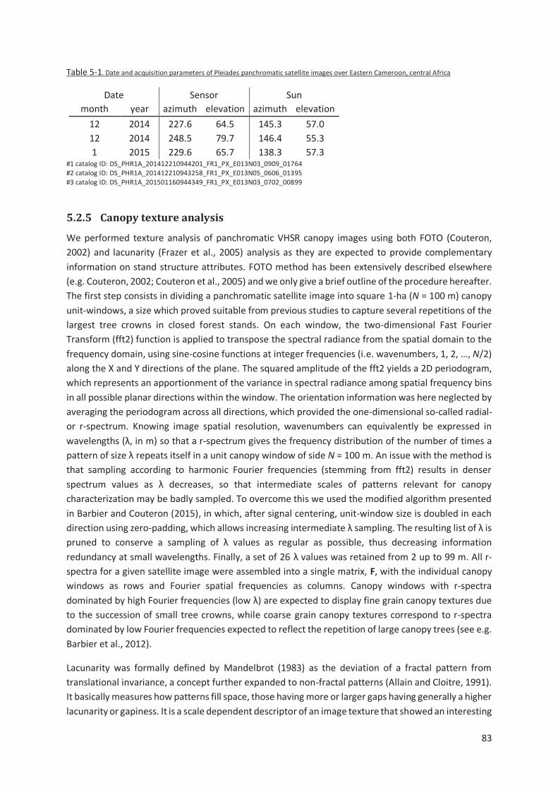
83
Table 5-1. Date and acquisition parameters of Pleiades panchromatic satellite images over Eastern Cameroon, central Africa
Date Sensor Sun
month year azimuth elevation azimuth elevation
12 2014 227.6 64.5 145.3 57.0
12 2014 248.5 79.7 146.4 55.3
1 2015 229.6 65.7 138.3 57.3 #1 catalog ID: DS_PHR1A_201412210944201_FR1_PX_E013N03_0909_01764 #2 catalog ID: DS_PHR1A_201412210943258_FR1_PX_E013N05_0606_01395 #3 catalog ID: DS_PHR1A_201501160944349_FR1_PX_E013N03_0702_00899
5.2.5 Canopy texture analysis
We performed texture analysis of panchromatic VHSR canopy images using both FOTO (Couteron,
2002) and lacunarity (Frazer et al., 2005) analysis as they are expected to provide complementary
information on stand structure attributes. FOTO method has been extensively described elsewhere
(e.g. Couteron, 2002; Couteron et al., 2005) and we only give a brief outline of the procedure hereafter.
The first step consists in dividing a panchromatic satellite image into square 1-ha (N = 100 m) canopy
unit-windows, a size which proved suitable from previous studies to capture several repetitions of the
largest tree crowns in closed forest stands. On each window, the two-dimensional Fast Fourier
Transform (fft2) function is applied to transpose the spectral radiance from the spatial domain to the
frequency domain, using sine-cosine functions at integer frequencies (i.e. wavenumbers, 1, 2, …, N/2)
along the X and Y directions of the plane. The squared amplitude of the fft2 yields a 2D periodogram,
which represents an apportionment of the variance in spectral radiance among spatial frequency bins
in all possible planar directions within the window. The orientation information was here neglected by
averaging the periodogram across all directions, which provided the one-dimensional so-called radial-
or r-spectrum. Knowing image spatial resolution, wavenumbers can equivalently be expressed in
wavelengths (λ, in m) so that a r-spectrum gives the frequency distribution of the number of times a
pattern of size λ repeats itself in a unit canopy window of side N = 100 m. An issue with the method is
that sampling according to harmonic Fourier frequencies (stemming from fft2) results in denser
spectrum values as λ decreases, so that intermediate scales of patterns relevant for canopy
characterization may be badly sampled. To overcome this we used the modified algorithm presented
in Barbier and Couteron (2015), in which, after signal centering, unit-window size is doubled in each
direction using zero-padding, which allows increasing intermediate λ sampling. The resulting list of λ is
pruned to conserve a sampling of λ values as regular as possible, thus decreasing information
redundancy at small wavelengths. Finally, a set of 26 λ values was retained from 2 up to 99 m. All r-
spectra for a given satellite image were assembled into a single matrix, F, with the individual canopy
windows as rows and Fourier spatial frequencies as columns. Canopy windows with r-spectra
dominated by high Fourier frequencies (low λ) are expected to display fine grain canopy textures due
to the succession of small tree crowns, while coarse grain canopy textures correspond to r-spectra
dominated by low Fourier frequencies expected to reflect the repetition of large canopy trees (see e.g.
Barbier et al., 2012).
Lacunarity was formally defined by Mandelbrot (1983) as the deviation of a fractal pattern from
translational invariance, a concept further expanded to non-fractal patterns (Allain and Cloitre, 1991).
It basically measures how patterns fill space, those having more or larger gaps having generally a higher
lacunarity or gapiness. It is a scale dependent descriptor of an image texture that showed an interesting
84
potential in forest studies to describe spatial variation in stand structure heterogeneity, notably related
to canopy openness (Frazer et al., 2005). In the present paper, we computed lacunarity following
Frazer et al. (2005) to which the reader should refer for more details. Lacunarity was computed in
canopy windows of size N = 100 m as Fourier r-spectra. On each unit-window, a moving square box of
size s (in pixels) is glided by one pixel at a time along all rows and columns. For each box of size s, the
mass, M, is computed as the sum of all pixels’ spectral radiance (previously normed per unit-window),
so that the probability distribution function Q(M,s) represents the frequency distribution of M divided
by the number of boxes at size s. The lacunarity statistic is then computed as ´*s, =µ¶*+,*>, 3µ¶*�,*>,4
+� , where µ¶*�,*>, and µ¶*+,*>, are the mean and mean of squared values of Q(M, s),
respectively. In our study we used 10 discrete box sizes, s, from 1 to 99 m, and normalized all lacunarity
values by dividing them by ∆(1). We then denote as a window lacunarity spectrum the series of
normalized lacunarity statistics computed at each box size for a given canopy window. All normalized
lacunarity spectra for a given satellite image were assembled into a single matrix, L, with the unit
canopy windows as rows and the box sizes as columns. The decreasing pattern of lacunarity with
increasing box size reflects the rate of increase in canopy heterogeneity from the finer to the coarser
scale patterns, which in the context of forest canopies is related to the degree of inter-crowns canopy
openness (see Frazer et al., 2005).
5.2.6 Statistical analyses
In order to systematically compare the canopy windows from a given satellite image, both the F table
of Fourier r-spectra, and the L table of lacunarity spectra were submitted independently to Principal
Component Analyses (PCA) as in Couteron et al. (2005) and Frazer et al. (2005). Columns’ normalization
prior to PCA (normed-PCA) allows uncovering texture gradients even when the absolute variation
between unit-windows is small. This led to independently synthetize the FOTO- and Lacunarity-texture
gradients present in the satellite images. From the 3D forest mockups, we extracted simple parameters
of stand structure and heterogeneity (listed in Table 2) in order to help the interpretation of texture
gradients produced by the two PCA. We then investigated the agreement between these two analyses
using a co-inertia analysis (COIA; Dolédec and Chessel, 1994, Dray et al. 2003). COIA is a simple and
robust method for the simultaneous analysis of two data tables matching by observations (here,
windows). Between two PCA, COIA is mathematically equivalent to the Inter-battery analysis of Tucker
(1958). The method maximizes the square covariance between the projected coordinates of the unit-
windows on the PCA axes of F and L. It thus simultaneously maximizes the variance in F and L separately
(the two PCA) and the correlation between the two sets of principal components. The texture gradients
captured by FOTO and by the lacunarity analysis can thus be projected on common orthogonal
components.
We then used window scores on the PCA or COIA analysis as independent texture indices in AGB
regression models. We used the Random Forest (RF) algorithm as implemented in the package
“randomForest” version 4.6.12 for R statistical software (R Core Team, 2016). RF is an ensemble of
learning methods for classification and regression based on decision trees (Breiman, 2001) increasingly
used in remote-sensing studies, notably for carbon mapping (Baccini et al., 2012; Mascaro et al., 2014;
Vieilledent et al., 2016). The aim is to overcome over-fitting problems that can occur using individual
decision trees. The algorithm builds a large number of decision trees that are trained on random
samples of both the training set (i.e. the observations) and the predictor variables, and outputs the
average of individual trees predictions. An interesting feature of such learning machine technics is that
85
it allows integrating a large number of variables of potentially different statistical distributions (Marvin
et al., 2016) and does not request specifying an explicit model form.
We evaluated regression model errors using the internal validation scheme of RF. At each run (n =
500), RF training set is by default composed of two thirds of the total number of observations, leaving
one third of the data to compute an independent estimate of model error, so-called “out-of-bag”
(OOB) error. A mean OOB model error over the 500 runs (±sd) is provided as pseudo R-squared (R2),
root-mean-square error (RMSE) and relative RMSE (rRMSE in %), along with the mean signed deviation
(MSD), used to compare local (i.e. per site) prediction bias in global (i.e. multi-site) models (Xu et al.,
2016).
Although RF have been developed to avoid overfitting (Breiman, 2001) it is not completely immune to
this problem (e.g. Mascaro et al., 2014). We thus assessed predictors’ importance using a built-in
metric denoted IncMSE (in %), which quantifies the percent increase in the mean MSE when predictors
are randomly permuted. We then applied a variable selection procedure using the VSURF package
(Genuer et al., 2015), which builds several RF models with increasing number of predictors, starting
with the most important ones (based on IncMSE) and retains the smallest significant model (see VSURF
description for computational details).
In this paper RF models were built to evaluate the potential of canopy texture to discriminate variations
in stand AGB among the full set of simulated canopy scenes. FOTO- and Lacunarity-texture indices
were first evaluated separately using windows scores from the two independent PCA (leading to the
F- and L-models, respectively). Both sources of texture information were then combined in a single RF
model using windows coordinates on the COIA axes (FL-model). Last, we added to the predictors a
bioclimatic proxy accounting for the regional variation in potential canopy height, as environmental
stress on forest growth has been shown to be a determining factor of pantropical variation in forest
AGB (Chave et al., 2014). This environmental stress variable E, a compound variable based on water
deficit, temperature seasonality and precipitation seasonality, is available as a global gridded layer at
2.5 arc sec resolution at http://chave.ups-tlse.fr/pantropical_allometry.htm (Chave et al., 2014) and
was used here as a proxy for forest potential height in a global model based on FOTO- and lacunarity-
textures (called FLE-model).
5.3 Results
5.3.1 Texture analysis of virtual canopy images
We applied both the FOTO method and the lacunarity analysis on all simulated canopy windows
generated from the 279 1-ha plots of tropical forest inventory. The plan 1-2 of the FOTO-PCA explained
53.5% (37% and 16.5% for axes 1 and 2, respectively) of the total textural variability among windows
r-spectra (F-table) and produced a typical correlation circle with spatial patterns sorted from short to
long wavelengths (or from high to low frequency wavenumbers) (Figure 5-1 A). Wavelengths (λ) of
about 5 to 10 m (visually relating to small crown sizes) were found on the positive side of the first PCA
axis (F-PCA1), intermediate λ (25 to 35 m) on the positive side of F-PCA2 and λ of 25 to 35 m (largest
crown sizes) on the negative side of F-PCA1. The ordination gradient on the first FOTO-PCA plan thus
corresponded to a fineness-coarseness canopy texture gradient, with aperiodic canopies found close
to the origin and heterogeneous ones (i.e. mixing small and large crown patches) found on the lower-
left part of the plan. The general decrease of canopy grain size along F-PCA1 negatively correlated with
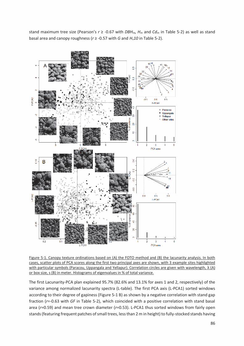
86
stand maximum tree size (Pearson’s r ≥ -0.67 with DBHm, Hm and Cdm in Table 5-2) as well as stand
basal area and canopy roughness (r ≥ -0.57 with G and Hv10 in Table 5-2).
Figure 5-1. Canopy texture ordinations based on (A) the FOTO method and (B) the lacunarity analysis. In both cases, scatter plots of PCA scores along the first two principal axes are shown, with 3 example sites highlighted with particular symbols (Paracou, Uppangala and Yellapur). Correlation circles are given with wavelength, λ (A) or box size, s (B) in meter. Histograms of eigenvalues in % of total variance.
The first Lacunarity-PCA plan explained 95.7% (82.6% and 13.1% for axes 1 and 2, respectively) of the
variance among normalized lacunarity spectra (L-table). The first PCA axis (L-PCA1) sorted windows
according to their degree of gapiness (Figure 5-1 B) as shown by a negative correlation with stand gap
fraction (r=-0.63 with GF in Table 5-2), which coincided with a positive correlation with stand basal
area (r=0.59) and mean tree crown diameter (r=0.53). L-PCA1 thus sorted windows from fairly open
stands (featuring frequent patches of small trees, less than 2 m in height) to fully-stocked stands having

87
a canopy made of larger trees. L-PCA2 captured variations in the rate of decrease in lacunarity with
box size, which reflected a gradient in canopy grain and heterogeneity. Fairly homogeneous canopy
(smooth canopy grain) characterized by a low rate of decrease in lacunarity with box size were found
on the negative side of L-PCA2, while heterogeneous canopy were found on the positive side of L-
PCA2. As a matter of fact, L-PCA2 was positively correlated with the canopy roughness index, Hv10
(r=0.7) and with maximum tree size (r=0.72 and 0.7 with Hm and DBHm, respectively). F-PCA1 and L-
PCA2 displayed a very high correlation of 0.93 (axes orientations are not informative in PCA) and
fundamentally depicted the same coarseness – fineness gradient of canopy aspect. On the other hand,
correlations between F-PCA2 and both Lacunarity-based PCA axes were weak, suggesting
complementarity.

88
Tab
le 5
-2.
Cor
rela
tion
bet
wee
n s
tan
d st
ruct
ure
par
amet
ers
extr
acte
d f
rom
th
ree
-dim
ensi
on
al m
ock
up
s an
d ca
no
py w
ind
ow
sco
res
on
the
text
ure
ord
inat
ion
axes
bas
ed o
n th
e FO
TO m
eth
od (
F-P
CA
1 an
d F-
PC
A2)
an
d th
e la
cun
arit
y an
alys
is (
L-P
CA
1 an
d L
-PC
A2)
. Pr
ob
abili
ty v
alu
e o
f Pe
arso
n co
rrel
atio
n t
est
are
pro
vid
ed b
etw
een
bra
cket
s an
d co
ded
fo
llow
ing
stan
dard
no
tati
on (
**
* P
≤ 0
.01
, *
* P
≤ 0
.01
, *
P ≤
0.0
5,
ns
= n
on
-sig
nif
ican
t).
St
and
str
uct
ure
par
amet
ers
F-P
CA
1 F-
PC
A2
L-P
CA
1 L-
PC
A2
GF
Gap
fra
ctio
n (c
um
ula
ted
area
of
pixe
ls <
2 m
in h
eigh
t)
0.04
(n
s)
-0.1
8 (*
**)
-0.6
3 (*
**)
0.12
(**
)
Hv1
0
Stan
dar
d d
evia
tio
n o
f m
axim
um
tre
e h
eigh
t am
ong
10
m q
uad
rats
-0
.6 (
***)
-0
.26
(***
) -0
.27
(***
) 0.
7 (*
**)
DB
Hm
St
and
max
imu
m t
ree
DB
H
-0.7
4 (*
**)
-0.2
1 (*
**)
0.17
(**
*)
0.7
(***
)
Hm
St
and
max
imu
m t
ree
hei
ght
-0.6
9 (*
**)
0.17
(**
*)
-0.1
(**
) 0.
72 (
***)
Cd
m
Stan
d m
axim
um
cro
wn
dia
met
er
-0.6
7 (*
**)
-0.3
(**
*)
0.17
(**
*)
0.64
(**
*)
N
Stan
d t
ree
den
sity
0.
08 (
*)
0.15
(**
*)
-0.0
1 (n
s)
-0.0
7 (.
)
G
Stan
d b
asal
are
a
-0.5
7 (*
**)
0.17
(**
*)
0.59
(**
*)
0.43
(**
*)
DB
Hm
ea
n
Qu
adra
tic
mea
n o
f tr
ee D
BH
-0
.46
(***
) 0.
06 (
.)
0.48
(**
*)
0.35
(**
*)
CD
me
an
Qu
adra
tic
mea
n o
f tr
ee c
row
ns
diam
eter
-0
.19
(***
) 0.
16 (
***)
0.
53 (
***)
0.
09 (
*)
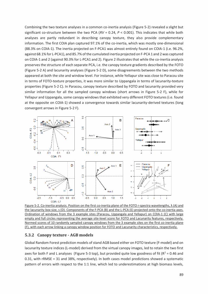
89
Combining the two texture analyses in a common co-inertia analysis (Figure 5-2) revealed a slight but
significant co-structure between the two PCA (RV = 0.24, P < 0.001). This indicates that while both
analyses are partly redundant in describing canopy texture, they also provide complementary
information. The first COIA plan captured 97.1% of the co-inertia, which was mostly one-dimensional
(88.3% on COIA-1). The inertia projected on F-PCA1 was almost entirely found on COIA-1 (i.e. 96.2%,
against 68.1% for L-PCA1), and 85.7% of the cumulated inertia projected on F-PCA 1 and 2 was captured
on COIA-1 and 2 (against 90.3% for L-PCA1 and 2). Figure 2 illustrates that while the co-inertia analysis
preserves the structure of each separate PCA, i.e. the canopy texture gradients described by the FOTO
(Figure 5-2 A) and lacunarity analyses (Figure 5-2 D), some disagreements between the two methods
appeared at both the site and window level. For instance, while Yellapur site was close to Paracou site
in terms of FOTO-texture properties, it was more similar to Uppangala in terms of lacunarity-texture
properties (Figure 5-2 C). In Paracou, canopy texture described by FOTO and lacunarity provided very
similar information for all the sampled canopy windows (short arrows in Figure 5-2 F), while for
Yellapur and Uppangala, some canopy windows that exhibited very different FOTO textures (i.e. found
at the opposite on COIA-1) showed a convergence towards similar lacunarity-derived textures (long
convergent arrows in Figure 5-2 F).
Figure 5-2. Co-inertia analysis. Position on the first co-inertia plane of the FOTO r-spectra wavelengths, λ (A) and the lacunarity box size, s (D). Components of the F-PCA (B) and the L-PCA (E) projected onto the co-inertia axes. Ordination of windows from the 3 example sites (Paracou, Uppangala and Yellapur) on COIA-1 (C) with large empty and full circles representing the average site-level score for FOTO and Lacunarity features, respectively. Normed scores of 10 randomly sampled canopy windows from the 3 example sites on the first co-inertia plane (F), with each arrow linking a canopy window position for FOTO and Lacunarity characteristics, respectively.
5.3.2 Canopy texture - AGB models
Global Random Forest prediction models of stand AGB based either on FOTO texture (F-model) and on
lacunarity texture indices (L-model) derived from the virtual canopy images, led to retain the two first
axes for both F and L analyses (Figure 5-3 top), but provided quite low goodness of fit (R2 = 0.46 and
0.31, with rRMSE = 31 and 38%, respectively). In both cases model predictions showed a systematic
pattern of errors with respect to the 1:1 line, which led to underestimations at high biomass levels,
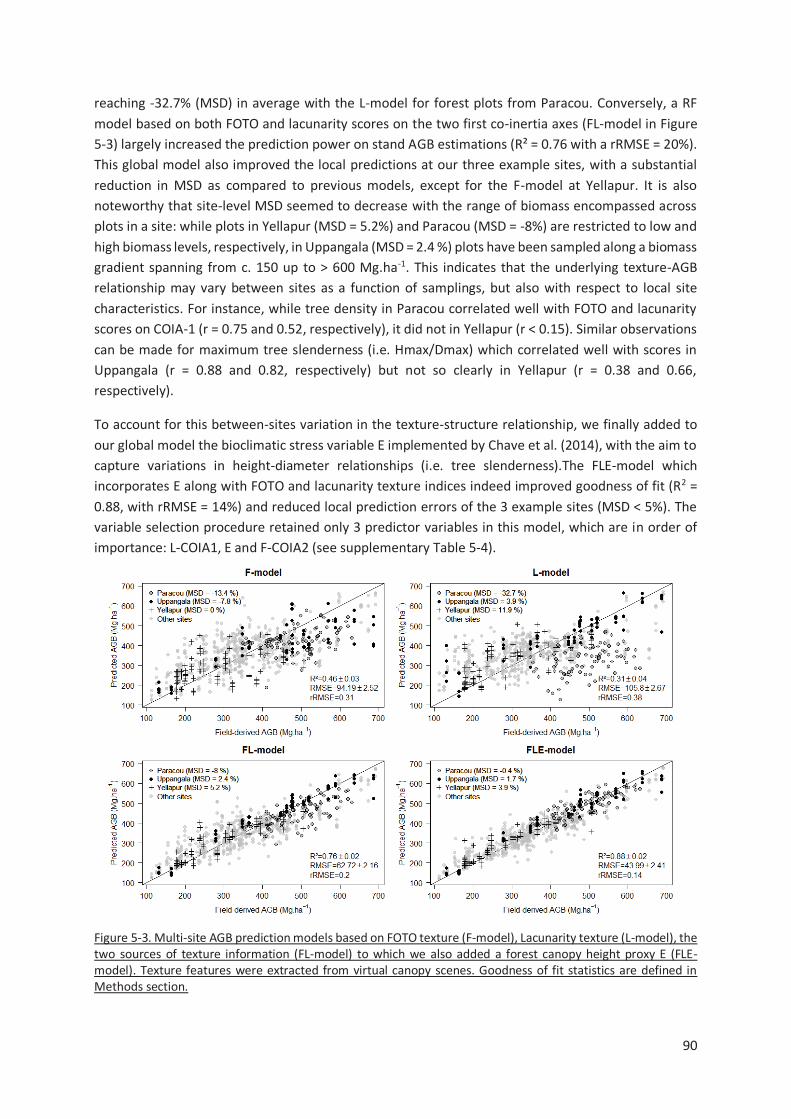
90
reaching -32.7% (MSD) in average with the L-model for forest plots from Paracou. Conversely, a RF
model based on both FOTO and lacunarity scores on the two first co-inertia axes (FL-model in Figure
5-3) largely increased the prediction power on stand AGB estimations (R² = 0.76 with a rRMSE = 20%).
This global model also improved the local predictions at our three example sites, with a substantial
reduction in MSD as compared to previous models, except for the F-model at Yellapur. It is also
noteworthy that site-level MSD seemed to decrease with the range of biomass encompassed across
plots in a site: while plots in Yellapur (MSD = 5.2%) and Paracou (MSD = -8%) are restricted to low and
high biomass levels, respectively, in Uppangala (MSD = 2.4 %) plots have been sampled along a biomass
gradient spanning from c. 150 up to > 600 Mg.ha-1. This indicates that the underlying texture-AGB
relationship may vary between sites as a function of samplings, but also with respect to local site
characteristics. For instance, while tree density in Paracou correlated well with FOTO and lacunarity
scores on COIA-1 (r = 0.75 and 0.52, respectively), it did not in Yellapur (r < 0.15). Similar observations
can be made for maximum tree slenderness (i.e. Hmax/Dmax) which correlated well with scores in
Uppangala (r = 0.88 and 0.82, respectively) but not so clearly in Yellapur (r = 0.38 and 0.66,
respectively).
To account for this between-sites variation in the texture-structure relationship, we finally added to
our global model the bioclimatic stress variable E implemented by Chave et al. (2014), with the aim to
capture variations in height-diameter relationships (i.e. tree slenderness).The FLE-model which
incorporates E along with FOTO and lacunarity texture indices indeed improved goodness of fit (R2 =
0.88, with rRMSE = 14%) and reduced local prediction errors of the 3 example sites (MSD < 5%). The
variable selection procedure retained only 3 predictor variables in this model, which are in order of
importance: L-COIA1, E and F-COIA2 (see supplementary Table 5-4).
Figure 5-3. Multi-site AGB prediction models based on FOTO texture (F-model), Lacunarity texture (L-model), the two sources of texture information (FL-model) to which we also added a forest canopy height proxy E (FLE-model). Texture features were extracted from virtual canopy scenes. Goodness of fit statistics are defined in Methods section.
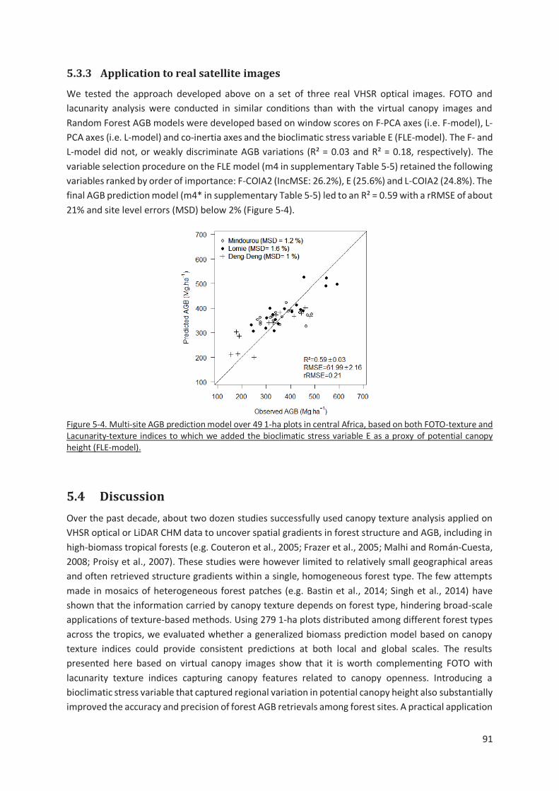
91
5.3.3 Application to real satellite images
We tested the approach developed above on a set of three real VHSR optical images. FOTO and
lacunarity analysis were conducted in similar conditions than with the virtual canopy images and
Random Forest AGB models were developed based on window scores on F-PCA axes (i.e. F-model), L-
PCA axes (i.e. L-model) and co-inertia axes and the bioclimatic stress variable E (FLE-model). The F- and
L-model did not, or weakly discriminate AGB variations (R² = 0.03 and R² = 0.18, respectively). The
variable selection procedure on the FLE model (m4 in supplementary Table 5-5) retained the following
variables ranked by order of importance: F-COIA2 (IncMSE: 26.2%), E (25.6%) and L-COIA2 (24.8%). The
final AGB prediction model (m4* in supplementary Table 5-5) led to an R² = 0.59 with a rRMSE of about
21% and site level errors (MSD) below 2% (Figure 5-4).
Figure 5-4. Multi-site AGB prediction model over 49 1-ha plots in central Africa, based on both FOTO-texture and Lacunarity-texture indices to which we added the bioclimatic stress variable E as a proxy of potential canopy height (FLE-model).
5.4 Discussion
Over the past decade, about two dozen studies successfully used canopy texture analysis applied on
VHSR optical or LiDAR CHM data to uncover spatial gradients in forest structure and AGB, including in
high-biomass tropical forests (e.g. Couteron et al., 2005; Frazer et al., 2005; Malhi and Román-Cuesta,
2008; Proisy et al., 2007). These studies were however limited to relatively small geographical areas
and often retrieved structure gradients within a single, homogeneous forest type. The few attempts
made in mosaics of heterogeneous forest patches (e.g. Bastin et al., 2014; Singh et al., 2014) have
shown that the information carried by canopy texture depends on forest type, hindering broad-scale
applications of texture-based methods. Using 279 1-ha plots distributed among different forest types
across the tropics, we evaluated whether a generalized biomass prediction model based on canopy
texture indices could provide consistent predictions at both local and global scales. The results
presented here based on virtual canopy images show that it is worth complementing FOTO with
lacunarity texture indices capturing canopy features related to canopy openness. Introducing a
bioclimatic stress variable that captured regional variation in potential canopy height also substantially
improved the accuracy and precision of forest AGB retrievals among forest sites. A practical application
92
of the method to a mosaic of real canopy images in the Congo basin showed that forest AGB inferences
could be made with high precision (i.e. c. 20% of error) up to 600 Mg.ha-1, i.e. without saturation.
5.4.1 Contrasted canopy texture - stand AGB relationships among sites
Global models based only on FOTO or lacunarity texture indices (F- and L-model, respectively)
significantly explained AGB variations but presented a relatively high uncertainty (rRMSE = 30-40%),
consistent with what other studies have reported for heterogeneous forest landscapes (e.g. Bastin et
al. 2014). To circumvent the problem and improve AGB inferences, previous empirical studies typically
used a forest type stratification step prior to the calibration of within-class texture–AGB models,
suggesting that the relationship is dependent on forest type (Bastin et al., 2014; Singh et al., 2014). We
indeed found that forest plots from different geographical sites were often clustered along the texture
gradients, generating systematic biases, and that texture indices did not always correlate with the
same stand structure parameters in different sites.
The relationship between FOTO-texture indices and forest AGB is expected to hold well for periodic
canopy patterns with homogeneous grain size (Proisy et al., 2007). In this ideal case, Fourier r-spectra
peak at the scale of the mean crown size of canopy trees (Barbier et al., 2010). Because crown size is
allometrically related to tree AGB (Jucker et al., 2016; Ploton et al., 2016) and that the 20 biggest trees
in 1-ha stands capture c. 85% of whole stands AGB variability in tropical forests (Bastin et al., 2015),
FOTO texture accurately predicts forest stand AGB. This is for instance the case along the successional
development pathway of mangrove tree cohorts (Proisy et al., 2007) but can also apply to mixed-
forests where the coarseness-fineness canopy texture gradient reflects difference in mature tree
statures (e.g. due to contrasting soil fertility, Couteron et al., 2005) or forest biomass gradients. At
Paracou study site for instance, a good linear correlation (r = -0.88) exists between tree density (N) and
the mean quadratic diameter (DBHmean) suggesting that sample plots align along a self-thinning
trajectory (see also Vincent et al., 2012). Our simulation procedure based on simple allometric
relationships thus produced fully-stocked virtual canopy images often displaying a periodic aspect (see
Figure 5-1) and for which a local F-model (i.e. based on FOTO texture only) provided very accurate AGB
predictions (rRMSE = c. 10%, results not shown). However, when the forest enters the gap phase
dynamics (Withmore, 1975), stand structure becomes heterogeneous in both the horizontal and
vertical dimensions, leading to higher canopy roughness, more frequent canopy gaps alternating with
clusters of large trees (e.g. Franklin et al., 2002; Guariguata and Ostertag, 2001; Spies, 1998). In
Uppangala for instance, where N and DBHmean did not correlate over the sampling plots (r = -0.09),
simulated canopy images were highly heterogeneous (see Figure 5-1), and a local L-model (i.e. based
on lacunarity texture only) produced more accurate AGB predictions (rRMSE< 10% vs. c. 20% with a
local F-model, results not shown). Other studies confirmed that lacunarity is an efficient method to
reveal canopy openness and heterogeneity gradients (e.g. Frazer et al., 2005; Malhi and Román-
Cuesta, 2008). It is therefore easy to understand that combining both types of texture indices largely
improved our multi-site prediction model (FL-model) at both the local and multi-site levels.
At the global scale however, variation in canopy height (Fayad et al., 2016; Saatchi et al., 2011) and
tree slenderness (Feldpausch et al., 2012), which proved critical for accurate AGB estimations (Chave
et al., 2014), cannot be directly accounted for by a 2D analysis of canopy texture, whatever the
method. Along a local forest successional gradient, canopy height variations follow increment in tree
size visible from above through the mean crown sizes. But, the maximal height reachable by dominant
trees is known to generally reveal the growth potential of a forest in relation to soil and regional
93
bioclimatic constraints, in particular with regard to water stress (Chave et al., 2014). Introducing the E
bioclimatic variable, which combines water deficit with temperature and precipitation seasonality (see
Chave et al., 2014) improved goodness of fit of our global regression model (FLE-model) and
significantly reduced local prediction errors.
On the set of real images from the Congo basin forest mosaic, the generalized texture-based model
was able to detect spatial variations in AGB within a tropical forest mosaic characterized by both high
AGB levels and forest types showing important variations in stand 3D structure, from closed-canopy
mixed-species mature stands to open-canopy Marantaceae forests. We have also shown here that the
multi-site FLE-model was the most robust with uncertainty of about 62 Mg.ha-1 at 1-ha scale (RMSE)
corresponding to a relative error of 21% (rRMSE). For such high-biomass forests, where the averaged
sampled plots AGB exceeds 350 Mg.ha-1 (i.e. 359±98), error levels reported here are only slightly higher
than those obtained from small-footprint airborne LiDAR (Zolkos et al., 2013). This result confirms and
expands the results previously obtained with a variety of satellite sensors (Quickbird, GeoEye, IKONOS,
SPOT-5), aerial images and even images freely available from the Google Earth engine (Bastin et al.,
2014; Meng et al., 2016; Ploton et al., 2012; Proisy et al., 2007; Singh et al., 2015, 2014) in temperate
or tropical forests. This represents an important step toward using VHSR optical imagery for broad-
scale assessments of forest AGB, as it eliminates the need of a preliminary forest classification (see for
instance Pargal et al., submitted). Recent progress also opened the perspective to perform texture
analysis on inter-calibrated satellite images from various sensors and/or in various configurations,
provided they partly overlap (Barbier and Couteron, 2015).
5.4.2 On 3D stand mockups and virtual canopy images for model calibration
Our stand modelling approach follows previously published studies on image texture simulations,
notably Barbier et al. (2012, 2010), Barbier and Couteron (2015) and Proisy et al. (2016). At the scale
of 1-ha forest plots, the size distribution of large objects within the scene (individual and aggregated
tree crowns) and their spatial arrangements (e.g. inter-crown gaps and associated shadows, variations
in tree density and size between subplots, etc.) are crucial determinants of spatial variations of the
apparent reflectance. Using a unique, simplified tree shape representation (i.e. cylindrical trunks and
non-plastic, ellipsoid crowns) allows generating sufficiently realistic brightness variation patterns at
those coarse scales for the interpretation of canopy texture gradients. For instance, Proisy et al. (2016)
showed that this approach allows producing texture r-spectra that have similar frequency peaks than
real ones over a wide range of mangrove successional stages. In the present study, a particular care
was taken to develop local tree size allometries and integrate field information on the spatial positions
of trees within stands, to mimic as well as possible the coarse-scale heterogeneity observed in real
field plots. This proved to be efficient to add consistent texture information related to the alternation
between patches of tree crowns and canopy gaps captured in high lacunarity values. However, our
stand simulation procedure could still be improved by accounting for crown plasticity (like for instance
in Boudon and Le Moguédec, 2007) or for between-species variations in trees inner-crown properties,
either geometric (e.g. foliage clumping and porosity, leaf angle distribution) or optical (Schneider et
al., 2014) that may influence grayscale variations at very small spatial scale. Considering these different
aspects is a long term research effort, and will likely benefit from technological advances in LiDAR
scanning and unmanned aerial vehicles (e.g. Morton and Cook, 2016). We suspect lacunarity analysis
to be more sensitive than FOTO to these geometric and optical parameters, making lacunarity a more
relevant complement to FOTO when analyzing simulated images than when analyzing real images.
94
An invaluable advantage of virtual canopy images is that they can be simulated in homogeneous
acquisition configurations on the basis of field data from different sites and regions. Texture indeed
quantifies pattern characteristics related to the contrasts between sunlit and shadowed surfaces and
is thus highly sensitive to the sun to sensor and scene angles (Barbier et al. 2011). Even if inter-
calibration procedures can help, particular configurations (e.g. backward scattering modes, near
hotspot directions) are intrinsically detrimental to canopy texture analysis and fatal to large-scale
applications over a mosaic of several images (Barbier and Couteron, 2015). On another hand,
programming image acquisition in controlled configurations, though possible, remains difficult,
sometimes costly and often very long, particularly over tropical zones where optical images frequently
suffer atmospheric pollutions related to dense cloud cover or persistent nebulosity. Another pitfall of
the detection of texture gradients through ordination is that the principal axes extracted from the data
are highly dependent on available samples and particular image sets may not reflect the entire possible
gradients of forest structure and canopy texture variations. In our example sites for instance, it clearly
appears that when the texture gradient is short, as was the case in Paracou, the texture-structure
relationship (as measured by R²) was not as strong as it was in areas covering a more extended gradient
(as in Uppangala). Simulated images thus allowed us to place all plots and sites along a large gradient
of canopy texture in order to stabilize the PCA axes and thus to increase robustness of the texture-
structure relationship, making it more universal than when fitted within sites. We therefore call for the
collaborative construction of a pantropical database of 3D forest mockups, that could be incremented
from plot data and local allometries in order to document all the particular situations encountered in
tropical forests. These mockups could then be processed with DART in homogeneous acquisition
conditions to produce arrays of canopy images of sufficient generality. The relevant simulated spectral
bands could finally be assembled according to the specific characteristics of any of the VHSR sensor
from which it could appear realistic to gather a very large array of real world, homogeneous images as
to perform global scale canopy texture analysis. This would be a way to consolidate the reference
gradients in canopy texture that emerged from our simulation results as to benchmark real
observations, i.e. for canopy texture analyses performed from real canopy images. This perspective is
a straightforward extension of the approach we introduced in the present paper, that would lead us
towards a tentative robust operational texture-structure relationship from which accurate
assessments of tropical forests AGB and carbon stocks could be produced.
Acknowledgments
Pierre Ploton was supported by an Erasmus Mundus PhD grant from the 2013–2016 Forest, Nature
and Society (FONASO) doctoral program. Satellite images were acquired through the Forest project
funded by the European Institute of Technology-Climate Knowledge & Innovation Community (grant
N° PIN0040_2015-3.1-044_P032_01-01). Forest inventory data were collected with the support of the
CoForTips project as part of the ERA-Net BiodivERsA 2011-2012 European joint call (ANR-12-EBID-
0002), the IRD project PPR FTH-AC “Changements globaux, biodiversité et santé en zone forestière
d’Afrique Centrale”, the IFPCAR project “Controlling for Uncertainty in Assessment of Forest
Aboveground Biomass in the Western Ghats of India” (grant N° 4509-1), Eramet, the World Bank,
WWF, the African Development Bank and the Center for Tropical Forest Science – Forest Global Earth
Observatory (CTFS-ForestGEO) of the Smithsonian Tropical Research Institute.
95
Author contributions. Conceived and designed the experiments: PP, NB and RP. Collected data (field
inventories): GD, VD, NGK, ML, GIIM, BS, NT, STM, DZD, NB and PP. Shared data: CMA, NA, NBal, NBar,
JFB, GC, DK, SP, PPe and DT. Analyzed the data: PP. Analysis feedback: RP, NB, MRM, JPG, PV and PC.
Wrote the paper: PP. Writing feedback: PC, NB, MRM, CP, UB and RP.
5.5 Reference
Allain, C., Cloitre, M., 1991. Characterizing the lacunarity of random and deterministic fractal sets. Phys. Rev. A 44, 3552.
Antin, C., Pélissier, R., Vincent, G., Couteron, P., 2013. Crown allometries are less responsive than stem allometry to tree size and habitat variations in an Indian monsoon forest. Trees 27, 1485–1495. doi:10.1007/s00468-013-0896-7
Asner, G.P., Martin, R.E., 2008. Spectral and chemical analysis of tropical forests: Scaling from leaf to canopy levels. Remote Sens. Environ. 112, 3958–3970.
Asner, G.P., Mascaro, J., Muller-Landau, H.C., Vieilledent, G., Vaudry, R., Rasamoelina, M., Hall, J.S., Breugel, M. van, 2011. A universal airborne LiDAR approach for tropical forest carbon mapping. Oecologia 168, 1147–1160. doi:10.1007/s00442-011-2165-z
Baccini, A., Goetz, S.J., Walker, W.S., Laporte, N.T., Sun, M., Sulla-Menashe, D., Hackler, J., Beck, P.S.A., Dubayah, R., Friedl, M.A., 2012. Estimated carbon dioxide emissions from tropical deforestation improved by carbon-density maps. Nat. Clim. Change 2, 182–185.
Barbier, N., Couteron, P., 2015. Attenuating the bidirectional texture variation of satellite images of tropical forest canopies. Remote Sens. Environ. 171, 245–260. doi:10.1016/j.rse.2015.10.007
Barbier, N., Couteron, P., Gastelly-Etchegorry, J.-P., Proisy, C., 2012. Linking canopy images to forest structural parameters: potential of a modeling framework. Ann. For. Sci. 69, 305–311. doi:10.1007/s13595-011-0116-9
Barbier, N., Couteron, P., Proisy, C., Malhi, Y., Gastellu-Etchegorry, J.-P., 2010. The variation of apparent crown size and canopy heterogeneity across lowland Amazonian forests. Glob. Ecol. Biogeogr. 19, 72–84.
Barbier, N., Proisy, C., Véga, C., Sabatier, D., Couteron, P., 2011. Bidirectional texture function of high resolution optical images of tropical forest: An approach using LiDAR hillshade simulations. Remote Sens. Environ. 115, 167–179.
Baskerville, G.L., 1972. Use of Logarithmic Regression in the Estimation of Plant Biomass. Can. J. For. Res. 2, 49–53. doi:10.1139/x72-009
Bastin, J.-F., Barbier, N., Couteron, P., Adams, B., Shapiro, A., Bogaert, J., De Cannière, C., 2014. Aboveground biomass mapping of African forest mosaics using canopy texture analysis: toward a regional approach. Ecol. Appl. 24, 1984–2001.
Bastin, J.-F., Barbier, N., Réjou-Méchain, M., Fayolle, A., Gourlet-Fleury, S., Maniatis, D., de Haulleville, T., Baya, F., Beeckman, H., Beina, D., 2015. Seeing Central African forests through their largest trees. Sci. Rep. 5. doi:doi:10.1038/srep13156
Boudon, F., Le Moguédec, G.L., 2007. Déformation asymétrique de houppiers pour la génération de représentations paysagères réalistes. Rev. Electron. Francoph. Inform. Graph. 1.
Breiman, L., 2001. Random forests. Mach. Learn. 45, 5–32. Broadbent, E.N., Asner, G.P., Peña-Claros, M., Palace, M., Soriano, M., 2008. Spatial partitioning of
biomass and diversity in a lowland Bolivian forest: Linking field and remote sensing measurements. For. Ecol. Manag. 255, 2602–2616. doi:10.1016/j.foreco.2008.01.044
Chave, J., Coomes, D., Jansen, S., Lewis, S.L., Swenson, N.G., Zanne, A.E., 2009. Towards a worldwide wood economics spectrum. Ecol. Lett. 12, 351–366. doi:10.1111/j.1461-0248.2009.01285.x
96
Chave, J., Muller-Landau, H.C., Baker, T.R., Easdale, T.A., Steege, H. ter, Webb, C.O., 2006. Regional and phylogenetic variation of wood density across 2456 neotropical tree species. Ecol. Appl. 16, 2356–2367. doi:10.1890/1051-0761(2006)016[2356:RAPVOW]2.0.CO;2
Chave, J., Réjou-Méchain, M., Búrquez, A., Chidumayo, E., Colgan, M.S., Delitti, W.B.C., Duque, A., Eid, T., Fearnside, P.M., Goodman, R.C., Henry, M., Martínez-Yrízar, A., Mugasha, W.A., Muller-Landau, H.C., Mencuccini, M., Nelson, B.W., Ngomanda, A., Nogueira, E.M., Ortiz-Malavassi, E., Pélissier, R., Ploton, P., Ryan, C.M., Saldarriaga, J.G., Vieilledent, G., 2014. Improved allometric models to estimate the aboveground biomass of tropical trees. Glob. Change Biol. 20, 3177–3190. doi:10.1111/gcb.12629
Chuyong, G.B., Condit, R., Kenfack, D., Losos, E.C., Moses, S.N., Songwe, N.C., Thomas, D.W., 2004. Korup forest dynamics plot, Cameroon. Trop. For. Divers. Dynamism 506–516.
Couteron, P., 2002. Quantifying change in patterned semi-arid vegetation by Fourier analysis of digitized aerial photographs. Int. J. Remote Sens. 23, 3407–3425.
Couteron, P., Pelissier, R., Nicolini, E.A., Paget, D., 2005. Predicting tropical forest stand structure parameters from Fourier transform of very high-resolution remotely sensed canopy images. J.
Appl. Ecol. 42, 1121–1128. DeFries, R., Achard, F., Brown, S., Herold, M., Murdiyarso, D., Schlamadinger, B., de Souza, C., 2007.
Earth observations for estimating greenhouse gas emissions from deforestation in developing countries. Environ. Sci. Policy 10, 385–394.
Dolédec, S., Chessel, D., 1994. Co-inertia analysis: an alternative method for studying species–
environment relationships. Freshw. Biol. 31, 277–294. Erdody, T.L., Moskal, L.M., 2010. Fusion of LiDAR and imagery for estimating forest canopy fuels.
Remote Sens. Environ. 114, 725–737. Fayad, I., Baghdadi, N., Guitet, S., Bailly, J.-S., Hérault, B., Gond, V., El Hajj, M., Minh, D.H.T., 2016.
Aboveground biomass mapping in French Guiana by combining remote sensing, forest inventories and environmental data. Int. J. Appl. Earth Obs. Geoinformation 52, 502–514.
Feldpausch, T.R., Lloyd, J., Lewis, S.L., Brienen, R.J., Gloor, M., Monteagudo Mendoza, A., Lopez-Gonzalez, G., Banin, L., Abu Salim, K., Affum-Baffoe, K., 2012. Tree height integrated into pantropical forest biomass estimates. Biogeosciences 3381–3403.
Franklin, J.F., Spies, T.A., Van Pelt, R., Carey, A.B., Thornburgh, D.A., Berg, D.R., Lindenmayer, D.B., Harmon, M.E., Keeton, W.S., Shaw, D.C., 2002. Disturbances and structural development of natural forest ecosystems with silvicultural implications, using Douglas-fir forests as an example. For. Ecol. Manag. 155, 399–423.
Frazer, G.W., Wulder, M.A., Niemann, K.O., 2005. Simulation and quantification of the fine-scale spatial pattern and heterogeneity of forest canopy structure: A lacunarity-based method designed for analysis of continuous canopy heights. For. Ecol. Manag. 214, 65–90.
Gastellu-Etchegorry, J.-P., Yin, T., Lauret, N., Cajgfinger, T., Gregoire, T., Grau, E., Feret, J.-B., Lopes, M., Guilleux, J., Dedieu, G., 2015. Discrete Anisotropic Radiative Transfer (DART 5) for modeling airborne and satellite spectroradiometer and LIDAR acquisitions of natural and urban landscapes. Remote Sens. 7, 1667–1701.
Genuer, R., Poggi, J.-M., Tuleau-Malot, C., 2015. VSURF: An R Package for Variable Selection Using Random Forests. R J. 7, 19–33.
Guariguata, M.R., Ostertag, R., 2001. Neotropical secondary forest succession: changes in structural and functional characteristics. For. Ecol. Manag. 148, 185–206.
Haralick, R.M., 1979. Statistical and structural approaches to texture. Proc. IEEE 67, 786–804. ICRAF, 2007. Wood density database. World Agrofor. Cent. Nairobi Kenya
http://db.worldagroforestry.org//wd. Jeyakumar, S., Ayyappan, N., Muthuramkumar, S., Rajarathinam, K., in press. Impacts of selective
logging on diversity, species composition and biomass of residual lowland dipterocarp forest in central Western Ghats, India. Trop. Ecol.
97
Jonckheere, I., Fleck, S., Nackaerts, K., Muys, B., Coppin, P., Weiss, M., Baret, F., 2004. Review of methods for in situ leaf area index determination: Part I. Theories, sensors and hemispherical photography. Agric. For. Meteorol. 121, 19–35.
Jucker, T., Caspersen, J., Chave, J., Antin, C., Barbier, N., Bongers, F., Dalponte, M., van Ewijk, K.Y., Forrester, D.I., Haeni, M., Higgins, S.I., Holdaway, R.J., Iida, Y., Lorimer, C., Marshall, P.L., Momo, S., Moncrieff, G.R., Ploton, P., Poorter, L., Rahman, K.A., Schlund, M., Sonké, B., Sterck, F.J., Trugman, A.T., Usoltsev, V.A., Vanderwel, M.C., Waldner, P., Wedeux, B.M.M., Wirth, C., Wöll, H., Woods, M., Xiang, W., Zimmermann, N.E., Coomes, D.A., 2016. Allometric equations for integrating remote sensing imagery into forest monitoring programmes. Glob. Change Biol. doi:10.1111/gcb.13388
Lu, D., 2006. The potential and challenge of remote sensing-based biomass estimation. Int. J. Remote
Sens. 27, 1297–1328. Lu, D., Chen, Q., Wang, G., Moran, E., Batistella, M., Zhang, M., Vaglio Laurin, G., Saah, D., 2012.
Aboveground Forest Biomass Estimation with Landsat and LiDAR Data and Uncertainty Analysis of the Estimates. Int. J. For. Res. 2012, 1–16. doi:10.1155/2012/436537
Malhi, Y., Román-Cuesta, R.M., 2008. Analysis of lacunarity and scales of spatial homogeneity in IKONOS images of Amazonian tropical forest canopies. Remote Sens. Environ. 112, 2074–2087.
Mandelbrot, B.B., 1983. The fractal geometry of nature. Macmillan. Marvin, D.C., Koh, L.P., Lynam, A.J., Wich, S., Davies, A.B., Krishnamurthy, R., Stokes, E., Starkey, R.,
Asner, G.P., 2016. Integrating technologies for scalable ecology and conservation. Glob. Ecol. Conserv. 7, 262–275. doi:10.1016/j.gecco.2016.07.002
Mascaro, J., Asner, G.P., Knapp, D.E., Kennedy-Bowdoin, T., Martin, R.E., Anderson, C., Higgins, M., Chadwick, K.D., 2014. A Tale of Two “Forests”: Random Forest Machine Learning Aids Tropical
Forest Carbon Mapping. PLoS ONE 9, e85993. doi:10.1371/journal.pone.0085993 Meng, S., Pang, Y., Zhang, Z., Jia, W., Li, Z., 2016. Mapping Aboveground Biomass using Texture Indices
from Aerial Photos in a Temperate Forest of Northeastern China. Remote Sens. 8, 230. doi:10.3390/rs8030230
Mermoz, S., Réjou-Méchain, M., Villard, L., Le Toan, T., Rossi, V., Gourlet-Fleury, S., 2015. Decrease of L-band SAR backscatter with biomass of dense forests. Remote Sens. Environ. 159, 307–317. doi:10.1016/j.rse.2014.12.019
Messinger, M., Asner, G., Silman, M., 2016. Rapid Assessments of Amazon Forest Structure and Biomass Using Small Unmanned Aerial Systems. Remote Sens. 8, 615. doi:10.3390/rs8080615
Morton, D.C., Cook, B.D., 2016. Amazon forest structure generates diurnal and seasonal variability in light utilization. Biogeosciences 13, 2195.
Olivas, P.C., Oberbauer, S.F., Clark, D.B., Clark, D.A., Ryan, M.G., O’Brien, J.J., Ordonez, H., 2013.
Comparison of direct and indirect methods for assessing leaf area index across a tropical rain forest landscape. Agric. For. Meteorol. 177, 110–116.
Pan, Y., Birdsey, R.A., Fang, J., Houghton, R., Kauppi, P.E., Kurz, W.A., Phillips, O.L., Shvidenko, A., Lewis, S.L., Canadell, J.G., 2011. A large and persistent carbon sink in the world’s forests. Science 333,
988–993. Pargal, S., Fararoda, R., Rajashekar, G., Balachandran, N., Réjou-Méchain, M., Barbier, N., Jha, C.S.,
Pélissier, R., Dadhwal, V.K., Couteron, P., n.d. Characterizing aboveground biomass – canopy texture relationships in a landscape of forest mosaic in the Western Ghats of India using very high resolution Cartosat Imagery. Remote Sens.
Ploton, P., Barbier, N., Takoudjou Momo, S., Réjou-Méchain, M., Boyemba Bosela, F., Chuyong, G., Dauby, G., Droissart, V., Fayolle, A., Goodman, R.C., Henry, M., Kamdem, N.G., Mukirania, J.K., Kenfack, D., Libalah, M., Ngomanda, A., Rossi, V., Sonké, B., Texier, N., Thomas, D., Zebaze, D., Couteron, P., Berger, U., Pélissier, R., 2016. Closing a gap in tropical forest biomass estimation: taking crown mass variation into account in pantropical allometries. Biogeosciences 13, 1571–
1585. doi:10.5194/bg-13-1571-2016
98
Ploton, P., Pélissier, R., Proisy, C., Flavenot, T., Barbier, N., Rai, S.N., Couteron, P., 2012. Assessing aboveground tropical forest biomass using Google Earth canopy images. Ecol. Appl. 22, 993–
1003. doi:10.1890/11-1606.1 Proisy, C., Couteron, P., Fromard, F., 2007. Predicting and mapping mangrove biomass from canopy
grain analysis using Fourier-based textural ordination of IKONOS images. Remote Sens. Environ. 109, 379–392.
Proisy, C., Féret, J.-B., Lauret, N., Gastellu-Etchegorry, J.-P., 2016. Mangrove forest dynamics using very high spatial resolution optical remote sensing., in: Remote Sensing of Land Surfaces: Urban and Coastal Area. N.N. Baghdadi & M. Zribi, Paris, pp. 274–300.
R Core Team, 2016. R: A language and environment for statistical computing. R Foundation for Statistical Computing, Vienna, Austria. URL https://www.R-project.org/.
Réjou-Méchain, M., Tymen, B., Blanc, L., Fauset, S., Feldpausch, T.R., Monteagudo, A., Phillips, O.L., Richard, H., Chave, J., 2015. Using repeated small-footprint LiDAR acquisitions to infer spatial and temporal variations of a high-biomass Neotropical forest. Remote Sens. Environ. 169, 93–
101. Saatchi, S.S., Harris, N.L., Brown, S., Lefsky, M., Mitchard, E.T., Salas, W., Zutta, B.R., Buermann, W.,
Lewis, S.L., Hagen, S., 2011. Benchmark map of forest carbon stocks in tropical regions across three continents. Proc. Natl. Acad. Sci. 108, 9899–9904.
Schneider, F.D., Leiterer, R., Morsdorf, F., Gastellu-Etchegorry, J.-P., Lauret, N., Pfeifer, N., Schaepman, M.E., 2014. Simulating imaging spectrometer data: 3D forest modeling based on LiDAR and in situ data. Remote Sens. Environ. 152, 235–250. doi:10.1016/j.rse.2014.06.015
Singh, M., Evans, D., Friess, D.A., Tan, B.S., Nin, C.S., 2015. Mapping Above-Ground Biomass in a Tropical Forest in Cambodia Using Canopy Textures Derived from Google Earth. Remote Sens. 7, 5057–5076. doi:10.3390/rs70505057
Singh, M., Malhi, Y., Bhagwat, S., 2014. Biomass estimation of mixed forest landscape using a Fourier transform texture-based approach on very-high-resolution optical satellite imagery. Int. J. Remote Sens. 35, 3331–3349. doi:10.1080/01431161.2014.903441
Slik, J.W., Paoli, G., McGuire, K., Amaral, I., Barroso, J., Bastian, M., Blanc, L., Bongers, F., Boundja, P., Clark, C., 2013. Large trees drive forest aboveground biomass variation in moist lowland forests across the tropics. Glob. Ecol. Biogeogr. 22, 1261–1271.
Spies, T.A., 1998. Forest structure: a key to the ecosystem. Northwest Sci. 72, 34–36. Stark, S.C., Enquist, B.J., Saleska, S.R., Leitold, V., Schietti, J., Longo, M., Alves, L.F., Camargo, P.B.,
Oliveira, R.C., 2015. Linking canopy leaf area and light environments with tree size distributions to explain Amazon forest demography. Ecol. Lett. n/a-n/a. doi:10.1111/ele.12440
Taubert, F., Jahn, M.W., Dobner, H.-J., Wiegand, T., Huth, A., 2015. The structure of tropical forests and sphere packings. Proc. Natl. Acad. Sci. 112, 15125–15129.
Tucker, L.R., 1958. An inter-battery method of factor analysis. Psychometrika 23, 111–136. Véga, C., Vepakomma, U., Morel, J., Bader, J.-L., Rajashekar, G., Jha, C.S., Ferêt, J., Proisy, C., Pélissier,
R., Dadhwal, V.K., 2015. Aboveground-Biomass Estimation of a Complex Tropical Forest in India Using Lidar. Remote Sens. 7, 10607–10625.
Vieilledent, G., Gardi, O., Grinand, C., Burren, C., Andriamanjato, M., Camara, C., Gardner, C.J., Glass, L., Rasolohery, A., Rakoto Ratsimba, H., Gond, V., Rakotoarijaona, J.-R., 2016. Bioclimatic envelope models predict a decrease in tropical forest carbon stocks with climate change in Madagascar. J. Ecol. 104, 703–715. doi:10.1111/1365-2745.12548
Vincent, G., Sabatier, D., Blanc, L., Chave, J., Weissenbacher, E., Pélissier, R., Fonty, E., Molino, J.-F., Couteron, P., 2012. Accuracy of small footprint airborne LiDAR in its predictions of tropical moist forest stand structure. Remote Sens. Environ. 125, 23–33.
Vincent, G., Sabatier, D., Rutishauser, E., 2014. Revisiting a universal airborne light detection and ranging approach for tropical forest carbon mapping: scaling-up from tree to stand to landscape. Oecologia 175, 439–443. doi:10.1007/s00442-014-2913-y
Withmore, T.C., 1975. Tropical rain forest of the far east. Claredon Prees Oxf. Univ. Prees Lond.

99
Xu, L., Saatchi, S.S., Yang, Y., Yu, Y., White, L., 2016. Performance of non-parametric algorithms for spatial mapping of tropical forest structure. Carbon Balance Manag. 11. doi:10.1186/s13021-016-0062-9
Zanne, A.E., Lopez-Gonzalez, G., Coomes, D.A., Ilic, J., Jansen, S., Lewis, S.L., Miller, R.B., Swenson, N.G., Wiemann, M.C., Chave, J., 2009. Data from: towards a worldwide wood economics spectrum. Dryad Digital Reposit.
Zhao, P., Lu, D., Wang, G., Wu, C., Huang, Y., Yu, S., 2016. Examining Spectral Reflectance Saturation in Landsat Imagery and Corresponding Solutions to Improve Forest Aboveground Biomass Estimation. Remote Sens. 8, 469. doi:10.3390/rs8060469
Zhou, J., Proisy, C., Descombes, X., Le Maire, G., Nouvellon, Y., Stape, J.-L., Viennois, G., Zerubia, J., Couteron, P., 2013. Mapping local density of young Eucalyptus plantations by individual tree detection in high spatial resolution satellite images. For. Ecol. Manag. 301, 129–141.
Zolkos, S.G., Goetz, S.J., Dubayah, R., 2013. A meta-analysis of terrestrial aboveground biomass estimation using lidar remote sensing. Remote Sens. Environ. 128, 289–298.
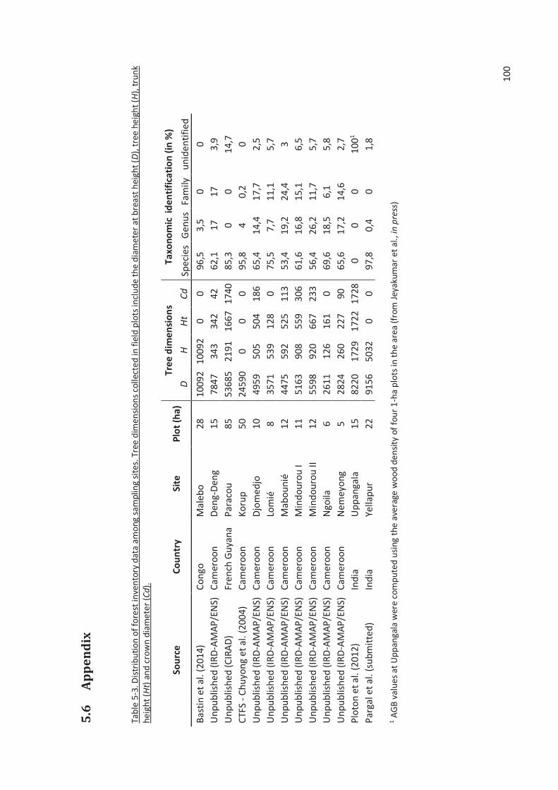
100
5
.6
Ap
pe
nd
ix
Tab
le 5
-3. D
istr
ibu
tio
n o
f fo
rest
inve
nto
ry d
ata
amo
ng s
ampl
ing
site
s. T
ree
dim
ensi
on
s co
llect
ed in
fie
ld p
lots
incl
ud
e th
e d
iam
eter
at
bre
ast
hei
ght
(D),
tre
e he
igh
t (H
), t
run
k h
eigh
t (H
t) a
nd
cro
wn
diam
eter
(C
d).
So
urc
e
Co
un
try
S
ite
P
lot
(ha
) T
ree
dim
en
sio
ns
Ta
xo
no
mic
id
en
tifi
cati
on
(in
%)
D
H
Ht
Cd
Sp
ecie
s G
enu
s Fa
mily
u
nid
enti
fied
Bas
tin
et
al. (
2014
) C
on
go
Mal
ebo
28
10
092
10
092
0
0 96
,5
3,5
0
0
Un
pu
blis
hed
(IR
D-A
MA
P/E
NS)
C
amer
oo
n D
eng-
Den
g 15
78
47
343
34
2
42
62,1
17
17
3,
9
Un
pu
blis
hed
(CIR
AD
) Fr
ench
Gu
yan
a P
arac
ou
85
53
685
21
91
1667
17
40
85,3
0
0 14
,7
CTF
S -
Ch
uyo
ng
et a
l. (2
004)
C
amer
oo
n K
oru
p
50
2459
0
0 0
0 95
,8
4 0,
2
0
Un
pu
blis
hed
(IR
D-A
MA
P/E
NS)
C
amer
oo
n D
jom
edjo
10
49
59
505
50
4
186
65
,4
14,4
17
,7
2,5
Un
pu
blis
hed
(IR
D-A
MA
P/E
NS)
C
amer
oo
n Lo
mié
8
3571
53
9
128
0
75,5
7,
7
11,1
5,
7
Un
pu
blis
hed
(IR
D-A
MA
P/E
NS)
C
amer
oo
n M
abo
un
ié
12
4475
59
2
525
11
3
53,4
19
,2
24,4
3
Un
pu
blis
hed
(IR
D-A
MA
P/E
NS)
C
amer
oo
n M
ind
ou
rou
I 11
51
63
908
55
9
306
61
,6
16,8
15
,1
6,5
Un
pu
blis
hed
(IR
D-A
MA
P/E
NS)
C
amer
oo
n M
ind
ou
rou
II
12
5598
92
0
667
23
3
56,4
26
,2
11,7
5,
7
Un
pu
blis
hed
(IR
D-A
MA
P/E
NS)
C
amer
oo
n N
goila
6
2611
12
6
161
0
69,6
18
,5
6,1
5,
8
Un
pu
blis
hed
(IR
D-A
MA
P/E
NS)
C
amer
oo
n N
emey
ong
5
2824
26
0
227
90
65
,6
17,2
14
,6
2,7
Plo
ton
et
al. (
2012
) In
dia
U
pp
anga
la
15
8220
17
29
1722
17
28
0 0
0 10
01
Par
gal e
t al
. (su
bmit
ted
) In
dia
Ye
llap
ur
22
9156
50
32
0 0
97,8
0,
4
0 1,
8
1 A
GB
val
ues
at
Up
pan
gala
wer
e co
mp
ute
d u
sing
the
ave
rage
wo
od
den
sity
of
fou
r 1
-ha
plo
ts in
th
e ar
ea (
from
Jey
akum
ar e
t al
., in
pre
ss)
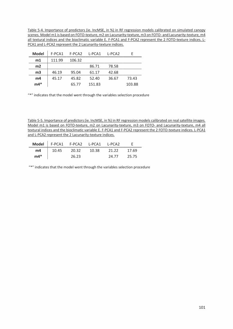
101
Table 5-4. Importance of predictors (ie. IncMSE, in %) in RF regression models calibrated on simulated canopy scenes. Model m1 is based on FOTO-texture, m2 on Lacunarity-texture, m3 on FOTO- and Lacunarity-texture, m4 all textural indices and the bioclimatic variable E. F-PCA1 and F-PCA2 represent the 2 FOTO-texture indices. L-PCA1 and L-PCA2 represent the 2 Lacunarity-texture indices.
Model F-PCA1 F-PCA2 L-PCA1 L-PCA2 E
m1 111.99 106.32 m2 86.71 78.58
m3 46.19 95.04 61.17 42.68
m4 45.17 45.82 52.40 36.67 73.43
m4* 65.77 151.83 103.88
“*” indicates that the model went through the variables selection procedure
Table 5-5. Importance of predictors (ie. IncMSE, in %) in RF regression models calibrated on real satellite images. Model m1 is based on FOTO-texture, m2 on Lacunarity-texture, m3 on FOTO- and Lacunarity-texture, m4 all textural indices and the bioclimatic variable E. F-PCA1 and F-PCA2 represent the 2 FOTO-texture indices. L-PCA1 and L-PCA2 represent the 2 Lacunarity-texture indices.
Model F-PCA1 F-PCA2 L-PCA1 L-PCA2 E
m4 10.45 20.32 10.38 21.22 17.69
m4* 26.23 24.77 25.75
“*” indicates that the model went through the variables selection procedure
102
6 GENERAL DISCUSSION In this chapter, I discuss the main findings, limits and perspectives of this thesis with respect to the
general thesis objective, which was to improve AGB estimations from field data (tree- and plot-level)
and RS data (landscape-level) using information on large trees structure, distribution and spatial
organization.
6.1 Estimation of forest AGB from field data
Field-derived estimations of AGB in forest sample plots constitute the bed rock of all forest AGB
monitoring methods (both non-spatial and spatial). Identifying the different sources of error associated
to those estimations, understanding the mechanisms behind those error sources and attempting to
mitigate them is of obvious relevance in the frame of the REDD program. In the current thesis, we
focused on the pantropical AGB model recently published in Chave et al. (2014) (of the form '() =01 " *$ " !+ " #,5) since this model, as its predecessor (Chave et al., 2005), is being widely employed
by international carbon scientists and managers. Chave et al. (2014) observed a systematic under-
estimation of AGB for large trees (≥ 30 Mg) with this model, which is an important drawback since
large trees compose most of stand-level AGB stocks (Bastin et al., 2015), drive spatial AGB variations
(Slik et al., 2013) and dominate stand-level AGB growth (Stephenson et al., 2014). A central objective
of the current work was to better understand the origin of this error, its consequences on forest stand
AGB estimations, and to propose a way to mitigate this error. To that end, we assembled a large set of
destructive data (i.e. measurements of trees dimensions and destructive estimates of trees AGB), in
which most of the largest trees came from our own field work, and studied whether the error pattern
of the pantropical model was related to variation in tree structure / morphology (i.e., with respect to
crown dimensions and crown contribution to tree AGB). Current allometric theories, in particular the
Metabolic Theory of Ecology (MTE), derive constant scaling exponent (7) of tree AGB with D and H
(hence D²H), at the cost of several simplifying assumptions made on the structure and topology of
trees branching network. Attempting to get further insights into what might cause the systematic error
on large trees in the pantropical model, we empirically assessed MTE’s set of simplifying assumptions,
which has not been done so far on large tropical trees and therefore constitute an original contribution
of this thesis. Last, the pantropical model error was propagated at the plot-level in tropical forests of
contrasted structure and composition, providing practical insights for model users. Overall, chapters 2
and 3 shed some light on the limits of the current pantropical model (and model form) and identify
potential improvement avenues.
6.1.1 Driver(s) of pantropical model bias on large trees
The pantropical model form is based on simple geometric arguments: tree mass is wood density (ρ)
multiplied by tree volume, and tree volume can be approximated by the volume of a simple geometric
solid i.e. D²H (Chave et al., 2005), leading to eq. 1. In equation 1, F is the whole-tree “form factor”
(Cannel et al. 1984) which defines the taper of the geometric shape (e.g. from a cylinder to a cone).
When equation 1 is adjusted to the data, we set a constant form factor to all trees. In practice, equation
2 is preferred (with b ≠ 1) because it provides a better statistical fit (Chave et al., 2005).
'() = 0· " $ " *!² " #, (eq. 1)
103
'() = 01 " *$ " !+ " #,5 (eq. 2)
In equation 2, the relationship between tree mass and the compound predictor variable is not
proportional i.e. we set a 7¸ increase of tree mass per 1% increase of $ " !+ " #, which can be
interpreted as a monotonic change of tree form as the tree change in mass. An important finding of
this thesis (chapter 2) is that the distribution of tree mass between trunk and crown is neither constant,
nor does it show a monotonic change along the tree mass gradient. This is particularly important
because the crown mass ratio (i.e. the proportion of tree aboveground mass in the crown) influences
the whole-tree form factor (Cannel et al. 1984). In our dataset (which includes most of the largest trees
used in Chave et al. 2014), the crown mass ratio was nearly constant up to a tree mass threshold of 10
Mg, then sharply increased with tree mass. Analyses in chapter 2 demonstrated that this non-linear
change in tree structure (i.e. shift in crown mass proportion after 10 Mg) is not capture by the
pantropical model and is responsible for the prediction bias observed on large trees. This finding
therefore leads us to a new question: is the observed change in tree structure a systematic,
biologically meaningful pattern, or is it a sampling artifact? In the former case, improving AGB
predictions accuracy on large trees would require modifying the form of the pantropical model. We
investigated alternative model forms and made a proposition along this line in chapter 2. In the latter
case, the prediction bias that we observe on large trees holds to a peculiarity in the structure of those
(sampled) trees and would decrease or disappear when the model is applied to a larger (more
representative) set of large trees.
The hypothesis of a sampling bias has been mentioned by Chave et al. (2014), whom rightfully argued
that a “majestic tree sampling bias” may occur, where scientists would preferentially select well-
conformed trees. The authors further noticed that most of the largest trees in their dataset were
selected in the frame of commercial logging activities (referring to the field work of this thesis), hence
those trees must have been particularly well-conformed. I would like to point out that the trees
collected in this thesis follow, but do not particularly steer the bias pattern observed in the pantropical
model (Figure 6-1). In our analyses, the increase of crown mass proportion among large trees was
indeed observed in all sampling sites (Figure 2-1) and was not a peculiarity of our Cameroonian dataset.
Confirming or ruling out the sampling bias hypothesis requires sampling more large trees (≥ 10 Mg),
which remain dramatically under-represented in the pantropical destructive dataset (c. 3%).
Ultimately, this would improve our knowledge of and ability to model pantropical trees biomass
allometry, and should therefore be a priority of future field campaigns. In this regard, methods to
extract tree volume and biomass from non-destructive terrestrial LiDAR scans are rapidly developing
(e.g. Calders et al., 2015; Hackenberg et al., 2014; Raumonen et al., 2013) and may soon revolutionize
tree AGB modelling strategies by considerably increasing the size and spatial representativity of tree
biomass reference datasets.
In thesis chapter 2, we hypothesized that the greater proportion of crown mass in large trees could
reflect an ontogenetic pattern associated to the process of tree crown metamorphosis. This
hypothesis goes against the MTE which, at the exception of size-dependent scaling between tree
diameter and length from seedling to sapling stages, predicts constant scaling exponents between tree
dimensions (and biomass) along tree ontogeny (Enquist et al., 2007; Niklas and Spatz, 2004). Yet,
several studies have documented changes in crown shape and allometric scaling with tree size among
trees > 10 cm D (e.g. Antin et al., 2013; Poorter et al., 2003; Smith et al., 2014). A well-documented
size-dependent change in crown allometric scaling is known as “crown liberation” (Cusset, 1980): upon
104
attaining the canopy, a typical tree decreases resources investment in height growth at the benefit of
lateral crown expansion, which can be interpreted as a strategy to enhance light capture (hence
maximize growth, Poorter et al., 2006) and/or shade and out-competed smaller neighbors (Sterck and
Bongers, 2001). Although ontogenetic shifts in allometric scaling of external crown dimensions (i.e.
crown diameter, depth) cannot be directly interpreted in terms of biomass, it is reasonable to think
that associated changes in inner crown structure (crown “metamorphosis” or “edification” through
reiteration, Hallé et al., 1978; Oldeman, 1974), changes in biomechanical constraints once the tree
reaches the upper canopy (notably due to wind exposure) and increased carbon allocation to
supporting tissues (Loehle, 2016) may modify whole-tree biomass scaling. None of these parameters
are included in the MTE, which – for example – implicitly assumes a constant access to light throughout
tree ontogeny.
Another hypothesis that has not been evocated in chapter 2 is that the crown mass ratio is dependent
of species traits, notably adult stature. Variation in tree allometric relationships with adult stature have
been widely documented (e.g. Antin et al., 2013; Bohlman and O’Brien, 2006; King, 1996; Sterck and
Bongers, 2001; Yang et al., 2015). In the destructive dataset, the increase of crown mass ratio above
10 Mg is driven by a few canopy and emergent tree species (i.e. capable of producing individuals > 10
Mg). Destructive data recently made available on the tallest African tree species (Entandrophragma
excelsum) confirm this trend with large E. excelsum individuals having high crown mass ratio (c. 80 %
for the largest sampled tree, Hemp et al., 2016) and following the bias pattern of the pantropical model
(star symbol in Figure 6-1). However, whether there is a non-linear, ontogenic increase of crown mass
ratio among large-stature species remain unclear. On Triplochiton scleroxylon for instance, a canopy
tree species for which enough individuals have been sampled so to look at species-specific trend in the
destructive database (i.e. 22 individuals from c. 6 to c. 47 Mg), we did not find any significant breaking-
point of crown mass ratio along tree mass. This could indicate that the non-linear increase of crown
mass ratio with tree mass applies when all species are pooled, but pooling species may mask species-
level patterns that are not necessarily non-linear. Under this hypothesis, it might be more efficient to
calibrate the pantropical model per group of species (e.g. based on adult stature) rather than changing
the model form.
Besides adult stature, considering species branching patterns might also be relevant to improve
pantropical biomass scaling relationships. In chapter 3, we found different scaling relationships
between daughter branches cross sections and parent branch cross-section (i.e. area ratio) among
species exhibiting different level of apical dominance (or frequency of branch segments along a central,
“principal” axis within the crown). Systematic differences in area ratio would, all else being equal,
impact species biomass scaling. Apical dominance is usually associated to species growth strategy (fast
growing pioneer-like vs slow-growing shade-tolerant species), as it favor faster height growth,
influence the overall crown shape (multi-layered vs mono-layered, respectively) and its efficiency at
gathering light in different conditions (bright vs shaded environments, respectively) (Horn, 2000,
1971). Among tree species studied in chapter 3, the pioneer to shade tolerant-like gradient that could
be established from species apical dominance was well supported by species-level wood density, with
a decreasing trend of wood density with increasing apical dominance (i.e. toward fast-growing, cheap-
wooded species). It is therefore possible that a species classification based on growth strategies along
the sun-shade gradient would capture different patterns of branch organization and associated
biomass scaling relationships. Documenting tropical tree species growth strategies and structural
development patterns represents a considerable amount of field work, but methodological
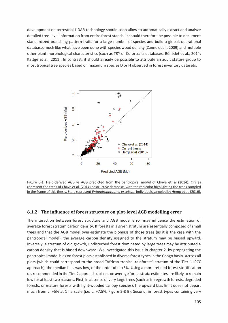
105
development on terrestrial LiDAR technology should soon allow to automatically extract and analyze
detailed tree-level information from entire forest stands. It should therefore be possible to document
standardized branching pattern-traits for a large number of species and build a global, operational
database, much like what have been done with species wood density (Zanne et al., 2009) and multiple
other plant morphological characteristics (such as TRY or Cofortraits databases, Bénédet et al., 2014;
Kattge et al., 2011). In contrast, it should already be possible to attribute an adult stature group to
most tropical tree species based on maximum species D or H observed in forest inventory datasets.
Figure 6-1. Field-derived AGB vs AGB predicted from the pantropical model of Chave et. al (2014). Circles represent the trees of Chave et al. (2014) destructive database, with the red color highlighting the trees sampled in the frame of this thesis. Stars represent Entandrophragma excelsum individuals sampled by Hemp et al. (2016).
6.1.2 The influence of forest structure on plot-level AGB modelling error
The interaction between forest structure and AGB model error may influence the estimation of
average forest stratum carbon density. If forests in a given stratum are essentially composed of small
trees and that the AGB model over-estimate the biomass of those trees (as it is the case with the
pantropical model), the average carbon density assigned to the stratum may be biased upward.
Inversely, a stratum of old growth, undisturbed forest dominated by large trees may be attributed a
carbon density that is biased downward. We investigated this issue in chapter 2, by propagating the
pantropical model bias on forest plots established in diverse forest types in the Congo basin. Across all
plots (which could correspond to the broad “African tropical rainforest” stratum of the Tier 1 IPCC
approach), the median bias was low, of the order of c. +5%. Using a more refined forest stratification
(as recommended in the Tier 2 approach), biases on average forest strata estimates are likely to remain
low for at least two reasons. First, in absence of very large trees (such as in regrowth forests, degraded
forests, or mature forests with light-wooded canopy species), the upward bias limit does not depart
much from c. +5% at 1 ha scale (i.e. c. +7.5%, Figure 2-8 B). Second, in forest types containing very
106
large trees (such as the Atlantic evergreen forests of western Cameroon), forest patches that are
mostly composed of very large trees are quiet rare (only 2 out of 130 1-ha plots in our dataset
underwent an under-estimation bias higher than -10%, Figure 2-8 B) and, therefore, should not have
much influence on average forest stratum carbon density. Our analyses therefore suggested that the
pantropical model bias should have relatively little impact on the estimation of forests carbon stock
(and stock change) derived from non-spatial monitoring methods (i.e. based on average carbon density
per forest strata). While non-spatial methods may provide an accurate estimation of forests carbon
stock at relatively large scales (e.g. national, regional), it is likely that spatially-explicit methods will
play a prominent role for forest monitoring in the near future, because of the much greater potential
of such methods to lower estimations uncertainties (and that at all spatial scales). Contrary to non-
spatial methods, spatially explicit carbon mapping methods (e.g. based on remote-sensing data) rely
on individual plot-level AGB estimations for signal calibration and should therefore be impacted by
plot-level bias. It is easily conceivable that a structure-dependent bias in calibration data would have
deleterious effects on our appraisal of a remote-sensing signal ability to discriminate AGB variations
(notably when the signal is directly linked to forest structure characteristics, such as crown size
repetitions or forest height), and eventually lead to an underestimation of remote-sensing signal error
and to a loss of prediction accuracy. On our dataset, the spread of biases at 1 ha scale was far from
being negligible (i.e. -15% to +7.7%) and increase when plot sized decreased (e.g. c. -20% to +10% at
0.25 ha scale), indicating that aerial LiDAR studies (which often use field plots ≤ 0.3 ha, e.g. Asner and
Mascaro, 2014) might be particularly sensitive to this issue. If the bias of the pantropical model does
not emerge from a sampling artifact (as discussed in the previous section), it should be included in
error propagation procedures and, given its impact of plot-level AGB estimations, efforts should be
made to mitigate it, for instance from complementary field measurements as proposed in chapter 2.
6.2 The influence of forest structure on the canopy texture – AGB
relationship
Part of this thesis dealt with the extrapolation of field-plot AGB via canopy texture features from very
high spatial resolution optical images. In chapter 4, I presented the Fourier Transform Ordination
(FOTO) method and gave a brief synthesis of empirical applications that have been made at local scale
(i.e. over a few hundreds square km) on diverse forest types and regions of the world. A major pitfall
of the method that emerged from chapter 4 is that the nature and strength of the information carried
by FOTO texture features on forest stand structure varies across forest types and sites. In other words,
the structure and spatial organization of trees in a forested area influence the relationship between
the emerging canopy texture (as described by FOTO) and forest stand structure parameters. In order
for canopy texture to be a useful source of information on forest carbon content at larger scale than
that of local case studies, it was necessary to identify and integrate the different factors influencing
the canopy texture – AGB relationship in the AGB regression model, so to stabilize model predictions
(i.e. across forest types and sites).
To that end, I adopted a simulation approach in chapter 5 and investigated how (simulated) canopy
texture features translated back into stand structure parameters in forests of contrasted structure and
dynamics across the tropics. Given the purpose of this analysis, using simulated forests and canopy
scenes was unavoidable, because acquiring real satellite images over multiple sites with a constraint
on acquisition angles is costly and, in some areas, simply unfeasible due to persistent clouds cover.
Despite the simplicity of trees 3D geometry in our simulations (symmetric, rounded crowns, notably),
107
this coarse level of realism proved sufficient to reconstruct FOTO canopy texture spectra in mangrove
forests (Proisy et al., 2016) and get consistent insights into instrumental effects on canopy texture
(Barbier et al., 2011; Barbier and Couteron, 2015). Among the different sampling sites that we studied
here, simulated Fourier texture features did not always correlate with the same structure parameters:
we often observed a good correlation with the mean tree diameter (Dg), but texture features
correlated with tree density (N) at some sites and with stand basal area (G) at others (results not shown
in chapter 5), which had consequences for AGB predictions. This instability between FOTO texture
metrics and stand structure parameters is consistent with past empirical case studies (chapter 4) and
confirms that the assemblage of simple lollipop-like trees is sufficient to study, at least to some extent,
the performance and limits of canopy texture-based indices in different ecological contexts, even in
terra firme forests which are more diverse and structurally complex than mangroves. The “lollipop-
tree” approach however reached its limits at some sites where we observed blatant deviations
between simulated texture and actual canopy texture in real satellite images. This was particularly the
case of Paracou’s forests, where individual trees in the highly packed canopy layer were easily
discernable in simulated canopies but much less so in real images (as canopy volume was entirely filled
with crowns). Using a rigid, simplified (ellipsoidal) crown representation leads to spatial distributions
of plant material that are unrealistically clustered (within crowns) and enhances the contrast between
shadowed and sunlit parts of tree crowns (Schneider et al., 2014), which artificially increases the
performance of texture-based indices in characterizing tree size distribution. FOTO texture on real
canopy images of Paracou’s forest is, for instance, much less informative on AGB variations that what
simulated canopy scenes suggested. Although several simplifying assumptions on tree geometry and
optical properties will require further attention in our simulation process (such as leaf area density and
its spatial distribution within stands and tree crowns, leaves angles, etc.), incorporating some plasticity
in crown shape stood out as the most important step to improve scenes realism.
When pooling all sites together, our analyses nonetheless showed that even with simplified tree
crowns shape, FOTO texture indices alone did not accurately capture forest AGB variations (Figure 5-3,
F-model). In closed-canopy conditions and when apparent crowns are of fairly homogeneous sizes
within unit canopy windows, FOTO texture characterizes the “mean” or “dominant” crown size, which
allometrically relates to Dg (e.g. Blanchard et al., 2016). FOTO texture indeed correlated well with Dg
variations in past case studies (e.g. Couteron et al., 2005; Ploton et al., 2012) as well as in most sites
studied in chapter 5. Dynamics of N, Dg and G (which is a strong predictor of AGB) along forest
development have been generalized in the well-known self-thinning theory (Reineke, 1933), which
predicts a gradual decrease of N and a concomitant increase of Dg and G as forest ages. The parameters
of self-thinning trajectories (intercept and slope) vary with tree crown and height allometric
relationships (Gül et al., 2005; Sterba and Monserud, 1993) which constrain the number of “average
trees” that can fit into a given area. If multi-specific canopy tree crown allometric relationships are
relatively stable across tropical forest sites (Blanchard et al., 2016), total forest height and tree height
allometry show important spatial variation driven by climate and soil (Banin et al., 2012; Chave et al.,
2014; Feldpausch et al., 2012; Ouédraogo et al., 2016), local topography (Yang et al., 2016) and stand
structure (Molto et al., 2014), notably. It is therefore not surprising that relationships between texture
features and stand structure varies across sites with local forest dynamics, local allometries and
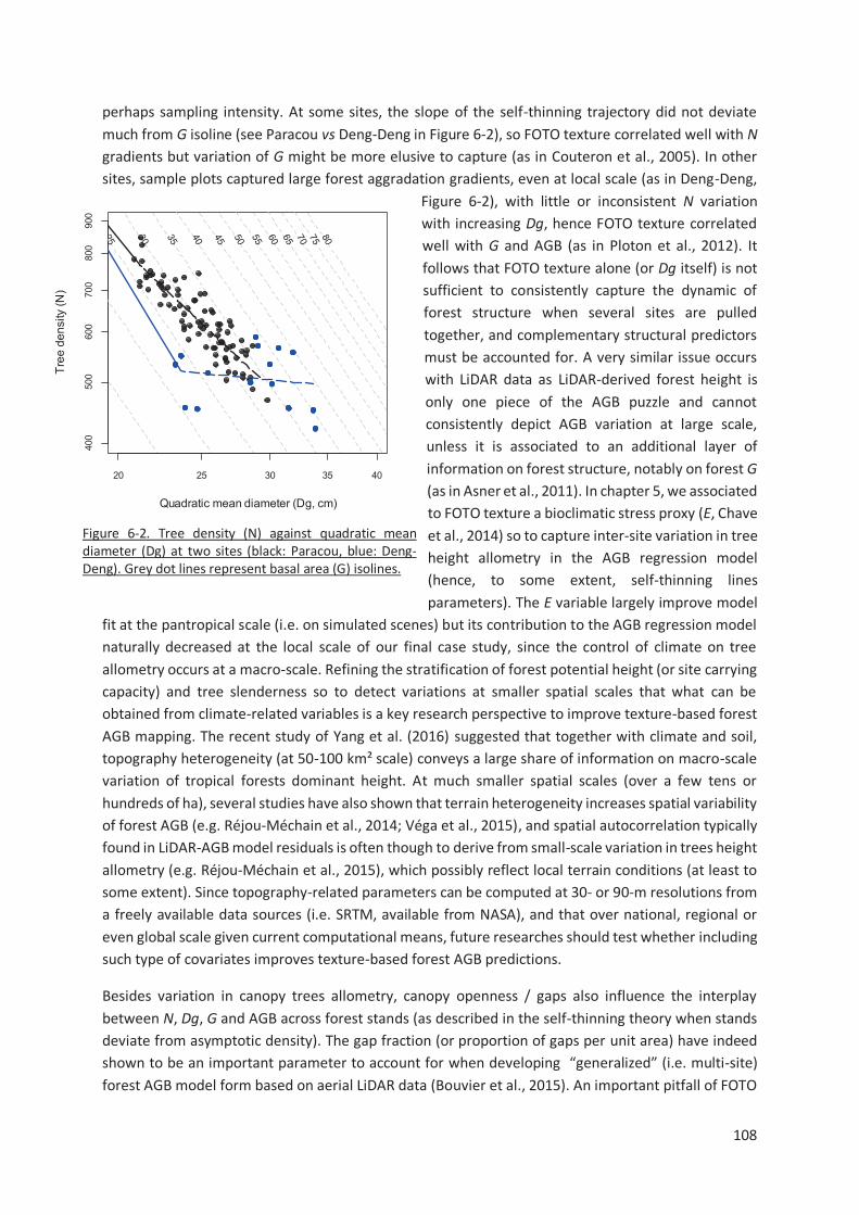
108
perhaps sampling intensity. At some sites, the slope of the self-thinning trajectory did not deviate
much from G isoline (see Paracou vs Deng-Deng in Figure 6-2), so FOTO texture correlated well with N
gradients but variation of G might be more elusive to capture (as in Couteron et al., 2005). In other
sites, sample plots captured large forest aggradation gradients, even at local scale (as in Deng-Deng,
Figure 6-2), with little or inconsistent N variation
with increasing Dg, hence FOTO texture correlated
well with G and AGB (as in Ploton et al., 2012). It
follows that FOTO texture alone (or Dg itself) is not
sufficient to consistently capture the dynamic of
forest structure when several sites are pulled
together, and complementary structural predictors
must be accounted for. A very similar issue occurs
with LiDAR data as LiDAR-derived forest height is
only one piece of the AGB puzzle and cannot
consistently depict AGB variation at large scale,
unless it is associated to an additional layer of
information on forest structure, notably on forest G
(as in Asner et al., 2011). In chapter 5, we associated
to FOTO texture a bioclimatic stress proxy (E, Chave
et al., 2014) so to capture inter-site variation in tree
height allometry in the AGB regression model
(hence, to some extent, self-thinning lines
parameters). The E variable largely improve model
fit at the pantropical scale (i.e. on simulated scenes) but its contribution to the AGB regression model
naturally decreased at the local scale of our final case study, since the control of climate on tree
allometry occurs at a macro-scale. Refining the stratification of forest potential height (or site carrying
capacity) and tree slenderness so to detect variations at smaller spatial scales that what can be
obtained from climate-related variables is a key research perspective to improve texture-based forest
AGB mapping. The recent study of Yang et al. (2016) suggested that together with climate and soil,
topography heterogeneity (at 50-100 km² scale) conveys a large share of information on macro-scale
variation of tropical forests dominant height. At much smaller spatial scales (over a few tens or
hundreds of ha), several studies have also shown that terrain heterogeneity increases spatial variability
of forest AGB (e.g. Réjou-Méchain et al., 2014; Véga et al., 2015), and spatial autocorrelation typically
found in LiDAR-AGB model residuals is often though to derive from small-scale variation in trees height
allometry (e.g. Réjou-Méchain et al., 2015), which possibly reflect local terrain conditions (at least to
some extent). Since topography-related parameters can be computed at 30- or 90-m resolutions from
a freely available data sources (i.e. SRTM, available from NASA), and that over national, regional or
even global scale given current computational means, future researches should test whether including
such type of covariates improves texture-based forest AGB predictions.
Besides variation in canopy trees allometry, canopy openness / gaps also influence the interplay
between N, Dg, G and AGB across forest stands (as described in the self-thinning theory when stands
deviate from asymptotic density). The gap fraction (or proportion of gaps per unit area) have indeed
shown to be an important parameter to account for when developing “generalized” (i.e. multi-site)
forest AGB model form based on aerial LiDAR data (Bouvier et al., 2015). An important pitfall of FOTO
20 25 30 35 40
400
500
600
700
800
900
Quadratic mean diameter (Dg, cm)
Tre
e d
en
sity (
N)
25 30 35 40 45 50 55 60 65 70 75 80Figure 6-2. Tree density (N) against quadratic mean diameter (Dg) at two sites (black: Paracou, blue: Deng-Deng). Grey dot lines represent basal area (G) isolines.
109
texture is that it cannot discriminate between tree crowns and gaps. Besides, forests canopies that are
too open (such as Maranthaceae forests) and/or heterogeneous in vertical and horizontal structure
usually display aperiodic canopy grains that are not properly characterized and discriminated by FOTO.
An important finding of our simulated experiment is that lacunarity analysis of canopy texture, which
have shown in our study and elsewhere to correlate with canopy openness and heterogeneity (Frazer
et al., 2005; Malhi and Román-Cuesta, 2008), provides an information that is complementary to FOTO
texture. Combining FOTO texture and lacunarity texture features indeed largely improved AGB model
fit across sites (Figure 5-3, FL-model), but also among some sites where FOTO alone led to poor results
(which was typically the case of aperiodic canopies from Yellapur, results not shown). This last result
is very encouraging. In some of the forest sites considered in chapter 5, structure parameters of sample
plots did not clearly represent self-thinning trajectories (as Deng-Deng in Figure 6-2) but rather
suggested forest landscapes composed of complex mosaics of patches undergoing different dynamics,
perhaps due to different times since last disturbance, variation in local species composition and/or
local abiotic conditions. These strong, local variations in forest structural profile (and emerging canopy
texture) go hand in hand with a high local variability in forest AGB, as observed in other mature tropical
forests (see for instance Guitet et al., 2015; Réjou-Méchain et al., 2014). When spatial changes in
canopy texture are not gradual in the landscape (contrary to mangrove forests, Proisy et al., 2007) but
rather a “salt-and-paper” mosaic of small patches, chances are that canopy texture intercepted by 1
ha unit windows display some level of heterogeneity. At the Uppangala site for example, Ploton et al.
(2012) reported a strong relationship between FOTO texture and AGB (R² of c. 0.78), but we specifically
targeted the few large forest patches (≥ 4-ha) displaying homogeneous grain size in the area to
establish calibration plots. This sampling strategy was motivated, at the time, by the will to mitigate
the effect plots geolocation error on texture-AGB relationship. I suspect however that it hided the
spurious effect of canopy heterogeneity on FOTO texture-AGB, and that the actual predictive accuracy
of the published model over the (heterogeneous) local forest mosaic is substantially lower than what
calibration fit metrics indicated. A similar issue occurs at several locations of south-eastern Cameroon
where the high heterogeneity of forests structure and texture at small spatial scales did not enable us
so far to find a significant relationship between FOTO texture features and stand AGB (pers. com. with
Dr. N. Barbier), which is in line with our final case studies of chapter 5 (i.e. when FOTO texture alone
was used). Although validating the added-value of the FOTO-lacunarity combination over the
traditional FOTO method will require multiple empirical assessments, the case study that we
performed confirmed the potential of the approach, as field plots AGB estimates were inferred with
reasonable accuracy and precision. If the approach proves relevant, an obvious step to take on would
be to propagate field plots AGB error into the texture-based model.
Over the past 15 years, canopy texture analysis from very high resolution (VHR) optical data have
demonstrated its ability to retrieve quantitative information on forest structure and AGB at local scale,
from various satellite sensors (Quickbird, GeoEye, IKONOS, SPOT-5) and aerial images (e.g. Bastin et
al., 2014; Ploton et al., 2012; Singh et al., 2015, 2014). In the study undertook in chapter 5, we clarified
some of the discrepancies observed between texture features and stand structure in past case studies,
and showed that it should be possible to develop a sounded, steady AGB inversion frame for broad
scale forest assessments. The recent launch of SPOT 6 and 7 (providing images up to 60 * 600 km in
stable configuration), the rapid deployment of cubesat constellations (suggesting that near-real time
VHR monitoring of Earth is not too far off, Marvin et al., 2016), the progress being made on
simultaneous texture analysis of multiple images (Barbier et al., 2011; Barbier and Couteron, 2015),
110
indicate that texture features from VHR imagery could play a key role in the REDD monitoring program.
Beyond the refinement of forest emission factors, producing fine resolution biomass maps at large
scale would help us improve our understanding of topical forest biomass variation and the relative
contribution of climate, soil, topography and disturbances at various scales.
6.3 Key thesis findings
The main results obtained in the present thesis are the following:
· The negative prediction bias of the pantropical tree biomass model on large trees pertains to
a systematic change in tree form with tree size: the contribution of crown to total tree mass
sharply increased on sampled trees ≥ 10 Mg (chapter 2) ;
· Accounting for proxies of crown dimensions (diameter, depth) allowed building an unbiased
generic tree biomass model, but it did not substantially increase model precision (chapter 2).
· Species with contrasted patterns of branch organization exhibited different scaling ;
relationships in crown structure (paper 3) ; this suggests that a classification based on how
species fill-in the 3D crown volume – in light of species growth strategies for example – may
be used to improve the precision of tree generic biomass models ;
· The bias of the pantropical tree biomass model propagates a systematic error at the plot level
that varies with stand structure (from c. -15 % to c. +8 % of mean plot biomass on our network
of 1-ha plots in central Africa) and increases as plot size decreases (up to c. -25 % for 0.1
subplots) (chapter 2) ; this error source (i.e. interaction between model error and stand
structure) is overlooked in published error propagation procedures ;
· Canopy textural properties from very high resolution optical images can be used to extrapolate
forest plot biomass estimations, but a simple simulation procedure showed that the nature
and strength of texture – biomass relationship varies between forest sites, in agreement with
previous empirical findings (chapter 4) ;
· Based on simulations of a large set of tropical forest plots, our analyses showed that (chapter
5) :
o While Fourier analysis of forest canopy images do not capture canopy openness,
lacunarity analysis does. Combining both types of analyses provided a more
comprehensive picture of forest structure, hence improved biomass predictions ;
o Accounting for a bioclimatic proxy of forest height, which cannot be retrieved from 2D
analyses of forest canopy images, further improved biomass model predictions ;
· While the classical Fourier-based analysis failed to predict forest biomass variations on a
mosaic of high-biomass forests in central Africa, our generalized biomass model gave an R² of
c. 0.6 and a RMSE of c. 62 Mg.ha-1 (chapter 5), suggesting that broad-scale monitoring of
tropical forests biomass from very-high resolution images may not be too far off.
111
6.4 Reference
Antin, C., Pélissier, R., Vincent, G., Couteron, P., 2013. Crown allometries are less responsive than stem allometry to tree size and habitat variations in an Indian monsoon forest. Trees 27, 1485–1495. doi:10.1007/s00468-013-0896-7
Asner, G.P., Mascaro, J., 2014. Mapping tropical forest carbon: Calibrating plot estimates to a simple LiDAR metric. Remote Sens. Environ. 140, 614–624.
Asner, G.P., Mascaro, J., Muller-Landau, H.C., Vieilledent, G., Vaudry, R., Rasamoelina, M., Hall, J.S., Breugel, M. van, 2011. A universal airborne LiDAR approach for tropical forest carbon mapping. Oecologia 168, 1147–1160. doi:10.1007/s00442-011-2165-z
Banin, L., Feldpausch, T.R., Phillips, O.L., Baker, T.R., Lloyd, J., Affum-Baffoe, K., Arets, E.J.M.M., Berry, N.J., Bradford, M., Brienen, R.J.W., Davies, S., Drescher, M., Higuchi, N., Hilbert, D.W., Hladik, A., Iida, Y., Salim, K.A., Kassim, A.R., King, D.A., Lopez-Gonzalez, G., Metcalfe, D., Nilus, R., Peh, K.S.-H., Reitsma, J.M., Sonké, B., Taedoumg, H., Tan, S., White, L., Wöll, H., Lewis, S.L., 2012. What controls tropical forest architecture? Testing environmental, structural and floristic drivers. Glob. Ecol. Biogeogr. 21, 1179–1190. doi:10.1111/j.1466-8238.2012.00778.x
Barbier, N., Couteron, P., 2015. Attenuating the bidirectional texture variation of satellite images of tropical forest canopies. Remote Sens. Environ. 171, 245–260. doi:10.1016/j.rse.2015.10.007
Barbier, N., Proisy, C., Véga, C., Sabatier, D., Couteron, P., 2011. Bidirectional texture function of high resolution optical images of tropical forest: An approach using LiDAR hillshade simulations. Remote Sens. Environ. 115, 167–179.
Bastin, J.-F., Barbier, N., Couteron, P., Adams, B., Shapiro, A., Bogaert, J., De Cannière, C., 2014. Aboveground biomass mapping of African forest mosaics using canopy texture analysis: toward a regional approach. Ecol. Appl. 24, 1984–2001.
Bastin, J.-F., Barbier, N., Réjou-Méchain, M., Fayolle, A., Gourlet-Fleury, S., Maniatis, D., de Haulleville, T., Baya, F., Beeckman, H., Beina, D., 2015. Seeing Central African forests through their largest trees. Sci. Rep. 5.
Bénédet, F., Vincke, D., Fayolle, A., Doucet, F., Gourlet-Fleury, S., 2014. Cofortraits, African plant traits information database. version 1.0 [WWW Document]. URL http://coforchan ge.cirad.fr/ african_plant_trait (accessed 1.1.16).
Blanchard, E., Birnbaum, P., Ibanez, T., Boutreux, T., Antin, C., Ploton, P., Vincent, G., Pouteau, R., Vandrot, H., Hequet, V., 2016. Contrasted allometries between stem diameter, crown area, and tree height in five tropical biogeographic areas. Trees 1–16.
Bohlman, S., O’Brien, S., 2006. Allometry, adult stature and regeneration requirement of 65 tree species on Barro Colorado Island, Panama. J. Trop. Ecol. 22, 123–136.
Bouvier, M., Durrieu, S., Fournier, R.A., Renaud, J.-P., 2015. Generalizing predictive models of forest inventory attributes using an area-based approach with airborne LiDAR data. Remote Sens. Environ. 156, 322–334. doi:10.1016/j.rse.2014.10.004
Calders, K., Newnham, G., Burt, A., Murphy, S., Raumonen, P., Herold, M., Culvenor, D., Avitabile, V., Disney, M., Armston, J., Kaasalainen, M., 2015. Nondestructive estimates of above-ground biomass using terrestrial laser scanning. Methods Ecol. Evol. 6, 198–208. doi:10.1111/2041-210X.12301
Chave, J., Andalo, C., Brown, S., Cairns, M.A., Chambers, J.Q., Eamus, D., Fölster, H., Fromard, F., Higuchi, N., Kira, T., Lescure, J.-P., Nelson, B.W., Ogawa, H., Puig, H., Riéra, B., Yamakura, T., 2005. Tree allometry and improved estimation of carbon stocks and balance in tropical forests. Oecologia 145, 87–99. doi:10.1007/s00442-005-0100-x
Chave, J., Réjou-Méchain, M., Búrquez, A., Chidumayo, E., Colgan, M.S., Delitti, W.B.C., Duque, A., Eid, T., Fearnside, P.M., Goodman, R.C., Henry, M., Martínez-Yrízar, A., Mugasha, W.A., Muller-Landau, H.C., Mencuccini, M., Nelson, B.W., Ngomanda, A., Nogueira, E.M., Ortiz-Malavassi, E., Pélissier, R., Ploton, P., Ryan, C.M., Saldarriaga, J.G., Vieilledent, G., 2014. Improved
112
allometric models to estimate the aboveground biomass of tropical trees. Glob. Change Biol. 20, 3177–3190. doi:10.1111/gcb.12629
Couteron, P., Pelissier, R., Nicolini, E.A., Paget, D., 2005. Predicting tropical forest stand structure parameters from Fourier transform of very high-resolution remotely sensed canopy images. J. Appl. Ecol. 42, 1121–1128.
Cusset, G., 1980. Sur des paramétres intervenant dans la croissance des arbres. La relation hauteur/diametre de l’axe primaire aerien. Candollea.
Enquist, B.J., Allen, A.P., Brown, J.H., Gillooly, J.F., Kerkhoff, A.J., Niklas, K.J., Price, C.A., West, G.B., 2007. Biological scaling: Does the exception prove the rule? Nature 445, E9–E10. doi:10.1038/nature05548
Feldpausch, T.R., Lloyd, J., Lewis, S.L., Brienen, R.J., Gloor, M., Monteagudo Mendoza, A., Lopez-Gonzalez, G., Banin, L., Abu Salim, K., Affum-Baffoe, K., 2012. Tree height integrated into pantropical forest biomass estimates. Biogeosciences 3381–3403.
Frazer, G.W., Wulder, M.A., Niemann, K.O., 2005. Simulation and quantification of the fine-scale spatial pattern and heterogeneity of forest canopy structure: A lacunarity-based method designed for analysis of continuous canopy heights. For. Ecol. Manag. 214, 65–90.
Guitet, S., Hérault, B., Molto, Q., Brunaux, O., Couteron, P., 2015. Spatial structure of above-ground biomass limits accuracy of carbon mapping in rainforest but large scale forest inventories can help to overcome. PloS One 10, e0138456.
Gül, A.U., Misir, M., Misir, N., Yavuz, H., 2005. Calculation of uneven-aged stand structures with the negative exponential diameter distribution and Sterba’s modified competition density rule.
For. Ecol. Manag. 214, 212–220. doi:10.1016/j.foreco.2005.04.012 Hackenberg, J., Morhart, C., Sheppard, J., Spiecker, H., Disney, M., 2014. Highly accurate tree models
derived from terrestrial laser scan data: A method description. Forests 5, 1069–1105. Hallé, F., Oldeman, R.A.A., Tomlinson, P.B., 1978. Tropical trees and forests: an architectural analysis.
Springer Verl. Berl. Heidelb. doi:10.1007/978-3-642-81190-6 Hemp, A., Zimmermann, R., Remmele, S., Pommer, U., Berauer, B., Hemp, C., Fischer, M., 2016. Africa’s
highest mountain harbours Africa’s tallest trees. Biodivers. Conserv. doi:10.1007/s10531-016-1226-3
Horn, H.S., 2000. Twigs, trees, and the dynamics of carbon in the landscape. Scaling Biol. 199–220. Horn, H.S., 1971. The adaptive geometry of trees. Princeton University Press. Kattge, J., Diaz, S., Lavorel, S., Prentice, I.C., Leadley, P., Bönisch, G., Garnier, E., Westoby, M., Reich,
P.B., Wright, I.J., 2011. TRY–a global database of plant traits. Glob. Change Biol. 17, 2905–2935. King, D.A., 1996. Allometry and life history of tropical trees. J. Trop. Ecol. 12, 25–44. Loehle, C., 2016. Biomechanical constraints on tree architecture. Trees. doi:10.1007/s00468-016-
1433-2 Malhi, Y., Román-Cuesta, R.M., 2008. Analysis of lacunarity and scales of spatial homogeneity in
IKONOS images of Amazonian tropical forest canopies. Remote Sens. Environ. 112, 2074–2087. Marvin, D.C., Koh, L.P., Lynam, A.J., Wich, S., Davies, A.B., Krishnamurthy, R., Stokes, E., Starkey, R.,
Asner, G.P., 2016. Integrating technologies for scalable ecology and conservation. Glob. Ecol. Conserv. 7, 262–275. doi:10.1016/j.gecco.2016.07.002
Molto, Q., Hérault, B., Boreux, J.-J., Daullet, M., Rousteau, A., Rossi, V., 2014. Predicting tree heights for biomass estimates in tropical forests – a test from French Guiana. Biogeosciences 11, 3121–
3130. doi:10.5194/bg-11-3121-2014 Niklas, K.J., Spatz, H.-C., 2004. Growth and hydraulic (not mechanical) constraints govern the scaling of
tree height and mass. Proc. Natl. Acad. Sci. U. S. A. 101, 15661–15663. Oldeman, R., 1974. L’architecture de la forêt guyanaise, Mémoires ORSTOM. ORSTOM, Paris. Ouédraogo, D.-Y., Fayolle, A., Gourlet-Fleury, S., Mortier, F., Freycon, V., Fauvet, N., Rabaud, S., Cornu,
G., Bénédet, F., Gillet, J.-F., Oslisly, R., Doucet, J.-L., Lejeune, P., Favier, C., 2016. The determinants of tropical forest deciduousness: disentangling the effects of rainfall and geology in central Africa. J. Ecol. doi:10.1111/1365-2745.12589
113
Ploton, P., Pélissier, R., Proisy, C., Flavenot, T., Barbier, N., Rai, S.N., Couteron, P., 2012. Assessing aboveground tropical forest biomass using Google Earth canopy images. Ecol. Appl. 22, 993–
1003. doi:10.1890/11-1606.1 Poorter, L., Bongers, F., Sterck, F.J., Wöll, H., 2003. Architecture of 53 rain forest tree species differing
in adult stature and shade tolerance. Ecology 84, 602–608. doi:10.1890/0012-9658(2003)084[0602:AORFTS]2.0.CO;2
Poorter, L., Bongers, L., Bongers, F., 2006. Architecture of 54 moist-forest tree species: traits, trade-offs, and functional groups. Ecology 87, 1289–1301. doi:10.1890/0012-9658(2006)87[1289:AOMTST]2.0.CO;2
Proisy, C., Couteron, P., Fromard, F., 2007. Predicting and mapping mangrove biomass from canopy grain analysis using Fourier-based textural ordination of IKONOS images. Remote Sens. Environ. 109, 379–392.
Proisy, C., Féret, J.-B., Lauret, N., Gastellu-Etchegorry, J.-P., 2016. Mangrove forest dynamics using very high spatial resolution optical remote sensing., in: Remote Sensing of Land Surfaces: Urban and Coastal Area. N.N. Baghdadi & M. Zribi, Paris, pp. 274–300.
Raumonen, P., Kaasalainen, M., Åkerblom, M., Kaasalainen, S., Kaartinen, H., Vastaranta, M., Holopainen, M., Disney, M., Lewis, P., 2013. Fast Automatic Precision Tree Models from Terrestrial Laser Scanner Data. Remote Sens. 5, 491–520. doi:10.3390/rs5020491
Reineke, L.H., 1933. Perfecting a stand-density index for even-aged forests. Réjou-Méchain, M., Muller-Landau, H.C., Detto, M., Thomas, S.C., Le Toan, T., Saatchi, S.S., Barreto-
Silva, J.S., Bourg, N.A., Bunyavejchewin, S., Butt, N., Brockelman, W.Y., Cao, M., Cárdenas, D., Chiang, J.-M., Chuyong, G.B., Clay, K., Condit, R., Dattaraja, H.S., Davies, S.J., Duque, A., Esufali, S., Ewango, C., Fernando, R.H.S., Fletcher, C.D., Gunatilleke, I.A.U.N., Hao, Z., Harms, K.E., Hart, T.B., Hérault, B., Howe, R.W., Hubbell, S.P., Johnson, D.J., Kenfack, D., Larson, A.J., Lin, L., Lin, Y., Lutz, J.A., Makana, J.-R., Malhi, Y., Marthews, T.R., McEwan, R.W., McMahon, S.M., McShea, W.J., Muscarella, R., Nathalang, A., Noor, N.S.M., Nytch, C.J., Oliveira, A.A., Phillips, R.P., Pongpattananurak, N., Punchi-Manage, R., Salim, R., Schurman, J., Sukumar, R., Suresh, H.S., Suwanvecho, U., Thomas, D.W., Thompson, J., Uríarte, M., Valencia, R., Vicentini, A., Wolf, A.T., Yap, S., Yuan, Z., Zartman, C.E., Zimmerman, J.K., Chave, J., 2014. Local spatial structure of forest biomass and its consequences for remote sensing of carbon stocks. Biogeosciences 11, 6827–6840. doi:10.5194/bg-11-6827-2014
Réjou-Méchain, M., Tymen, B., Blanc, L., Fauset, S., Feldpausch, T.R., Monteagudo, A., Phillips, O.L., Richard, H., Chave, J., 2015. Using repeated small-footprint LiDAR acquisitions to infer spatial and temporal variations of a high-biomass Neotropical forest. Remote Sens. Environ. 169, 93–
101. Schneider, F.D., Leiterer, R., Morsdorf, F., Gastellu-Etchegorry, J.-P., Lauret, N., Pfeifer, N., Schaepman,
M.E., 2014. Simulating imaging spectrometer data: 3D forest modeling based on LiDAR and in situ data. Remote Sens. Environ. 152, 235–250. doi:10.1016/j.rse.2014.06.015
Singh, M., Evans, D., Friess, D.A., Tan, B.S., Nin, C.S., 2015. Mapping Above-Ground Biomass in a Tropical Forest in Cambodia Using Canopy Textures Derived from Google Earth. Remote Sens. 7, 5057–5076. doi:10.3390/rs70505057
Singh, M., Malhi, Y., Bhagwat, S., 2014. Biomass estimation of mixed forest landscape using a Fourier transform texture-based approach on very-high-resolution optical satellite imagery. Int. J. Remote Sens. 35, 3331–3349. doi:10.1080/01431161.2014.903441
Slik, J.W., Paoli, G., McGuire, K., Amaral, I., Barroso, J., Bastian, M., Blanc, L., Bongers, F., Boundja, P., Clark, C., 2013. Large trees drive forest aboveground biomass variation in moist lowland forests across the tropics. Glob. Ecol. Biogeogr. 22, 1261–1271.
Smith, D.D., Sperry, J.S., Enquist, B.J., Savage, V.M., McCulloh, K.A., Bentley, L.P., 2014. Deviation from symmetrically self-similar branching in trees predicts altered hydraulics, mechanics, light interception and metabolic scaling. New Phytol. 201, 217–229. doi:10.1111/nph.12487
Stephenson, N.L., Das, A.J., Condit, R., Russo, S.E., Baker, P.J., Beckman, N.G., Coomes, D.A., Lines, E.R., Morris, W.K., Rüger, N., Álvarez, E., Blundo, C., Bunyavejchewin, S., Chuyong, G., Davies, S.J.,
114
Duque, Á., Ewango, C.N., Flores, O., Franklin, J.F., Grau, H.R., Hao, Z., Harmon, M.E., Hubbell, S.P., Kenfack, D., Lin, Y., Makana, J.-R., Malizia, A., Malizia, L.R., Pabst, R.J., Pongpattananurak, N., Su, S.-H., Sun, I.-F., Tan, S., Thomas, D., van Mantgem, P.J., Wang, X., Wiser, S.K., Zavala, M.A., 2014. Rate of tree carbon accumulation increases continuously with tree size. Nature 507, 90–93. doi:10.1038/nature12914
Sterba, H., Monserud, R.A., 1993. The maximum density concept applied to uneven-aged mixed-species stands. For. Sci. 39, 432–452.
Sterck, F.J., Bongers, F., 2001. Crown development in tropical rain forest trees: patterns with tree height and light availability. J. Ecol. 89, 1–13. doi:10.1046/j.1365-2745.2001.00525.x
Véga, C., Vepakomma, U., Morel, J., Bader, J.-L., Rajashekar, G., Jha, C.S., Ferêt, J., Proisy, C., Pélissier, R., Dadhwal, V.K., 2015. Aboveground-Biomass Estimation of a Complex Tropical Forest in India Using Lidar. Remote Sens. 7, 10607–10625.
Yang, X.-D., Yan, E.-R., Chang, S.X., Da, L.-J., Wang, X.-H., 2015. Tree architecture varies with forest succession in evergreen broad-leaved forests in Eastern China. Trees 29, 43–57. doi:10.1007/s00468-014-1054-6
Yang, Y., Saatchi, S., Xu, L., Yu, Y., Lefsky, M., White, L., Knyazikhin, Y., Myneni, R., 2016. Abiotic Controls on Macroscale Variations of Humid Tropical Forest Height. Remote Sens. 8, 494. doi:10.3390/rs8060494
Zanne, A.E., Lopez-Gonzalez, G., Coomes, D.A., Ilic, J., Jansen, S., Lewis, S.L., Miller, R.B., Swenson, N.G., Wiemann, M.C., Chave, J., 2009. Global wood density database.

I
Résumé étendu (Extended summary in French)
Amélioration des estimations de biomasse des forêts tropicales : apport de la
structure et de l’organisation spatiale des arbres de canopée
Pierre Ploton
IRD-UMR AMAP/ AgroParisTech, Montpellier (France)
Technische Universitat Dresden (Allemagne)
Mots clés : carbone forestier, REDD, modèle de biomasse pantropical, structure de canopée, texture de
canopée, imagerie optique passive, transformée de Fourier, lacunarité
Introduction
L’inquiétude grandissante autour des effets du changement climatique global a mené à l’émergence de
politiques internationales visant à suivre et à gérer durablement les stocks de carbone séquestrés par la
végétation terrestre, et en particulier par les forêts tropicales (REDD+). La déforestation et la dégradation
de ces forêts associées au développement économique des pays sont en effet considérées comme étant
la deuxième source la plus importante d’émission de dioxyde de carbone d’origine anthropique de ces
dernières décennies. L’initiative REDD+ repose en partie sur notre capacité à quantifier avec exactitude
et précision les stocks de carbone forestier à diverses échelles spatiales (ex. province, pays, bassin
forestier), et ce de façon répétée (suivi temporel), ce qui constitue un chalenge scientifique et technique
majeur. Une approche classique consiste à cartographier le carbone forestier, ou la biomasse forestière
épigée (AGB, un proxy fréquemment utilisé), en extrapolant des estimations d’AGB locales (i.e. réalisées
au sein de parcelles d’inventaire, étape 1) au moyen de données de télédétection (étape 2). Ces deux
étapes impliquent l’utilisation de modèles biophysiques plus ou moins performants dont les erreurs, qui
ne sont pas totalement connues et maitrisées, se propagent jusqu’aux estimations finales. L’amélioration
des ces modèles soulève un certain nombre de questions à l’interface entre la biomécanique,
l’architecture et l’écologie des espèces d’arbre, l’organisation des peuplements forestiers et le traitement
du signal, notamment. Dans cette thèse, nous nous sommes intéressés aux deux étapes de la chaine de
traitement en focalisant notre attention sur les grands arbres de canopée. Cette attention particulière
nous est apparue pertinente à la fois parce que les grands arbres représentent la majeure partie de la
biomasse d’un peuplement forestier mais également parce que ces arbres sont visibles sur les images
satellitaires optiques utilisées dans ce travail.
Deux objectifs principaux ont guidé notre étude. Le premier était de mieux comprendre la contribution
des grands arbres à l’erreur d’un modèle pantropical de biomasse populaire au sein de la communauté
scientifique internationale et de mieux intégrer leurs particularités structurelles dans un nouveau modèle.
Le deuxième objectif visait à améliorer une méthode d’extrapolation de la biomasse basée sur les
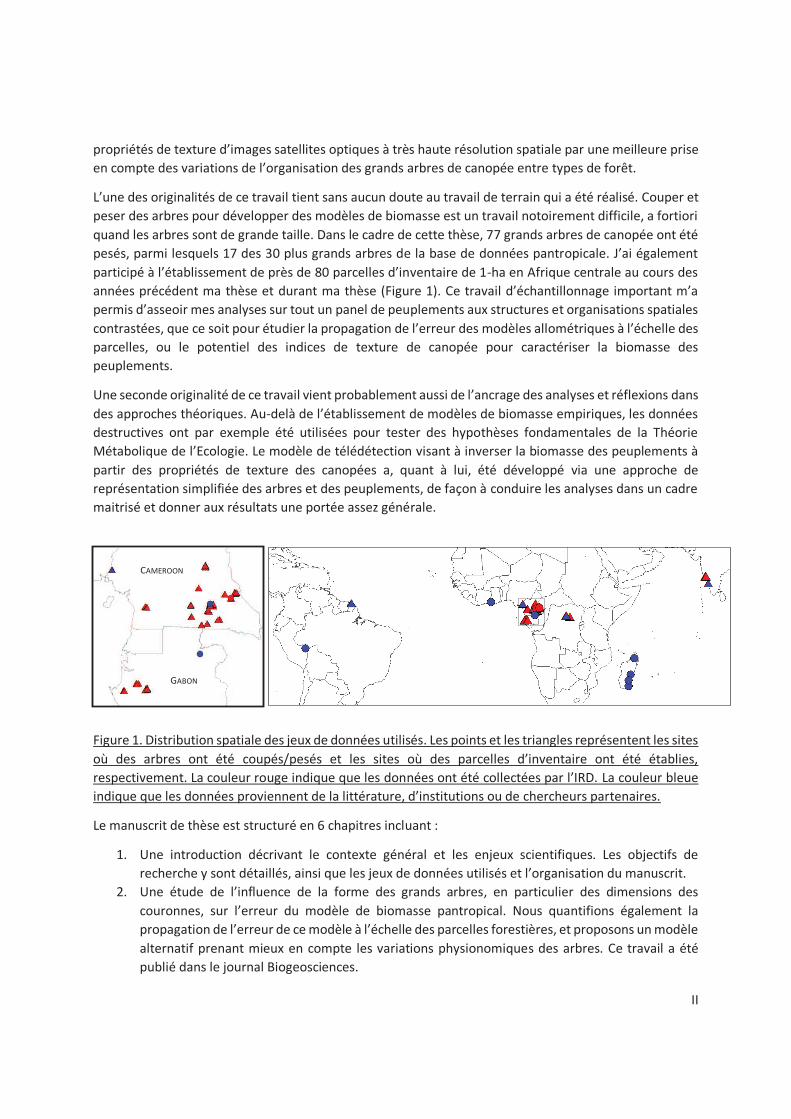
II
propriétés de texture d’images satellites optiques à très haute résolution spatiale par une meilleure prise
en compte des variations de l’organisation des grands arbres de canopée entre types de forêt.
L’une des originalités de ce travail tient sans aucun doute au travail de terrain qui a été réalisé. Couper et
peser des arbres pour développer des modèles de biomasse est un travail notoirement difficile, a fortiori
quand les arbres sont de grande taille. Dans le cadre de cette thèse, 77 grands arbres de canopée ont été
pesés, parmi lesquels 17 des 30 plus grands arbres de la base de données pantropicale. J’ai également
participé à l’établissement de près de 80 parcelles d’inventaire de 1-ha en Afrique centrale au cours des
années précédent ma thèse et durant ma thèse (Figure 1). Ce travail d’échantillonnage important m’a
permis d’asseoir mes analyses sur tout un panel de peuplements aux structures et organisations spatiales
contrastées, que ce soit pour étudier la propagation de l’erreur des modèles allométriques à l’échelle des
parcelles, ou le potentiel des indices de texture de canopée pour caractériser la biomasse des
peuplements.
Une seconde originalité de ce travail vient probablement aussi de l’ancrage des analyses et réflexions dans
des approches théoriques. Au-delà de l’établissement de modèles de biomasse empiriques, les données
destructives ont par exemple été utilisées pour tester des hypothèses fondamentales de la Théorie
Métabolique de l’Ecologie. Le modèle de télédétection visant à inverser la biomasse des peuplements à
partir des propriétés de texture des canopées a, quant à lui, été développé via une approche de
représentation simplifiée des arbres et des peuplements, de façon à conduire les analyses dans un cadre
maitrisé et donner aux résultats une portée assez générale.
Figure 1. Distribution spatiale des jeux de données utilisés. Les points et les triangles représentent les sites
où des arbres ont été coupés/pesés et les sites où des parcelles d’inventaire ont été établies,
respectivement. La couleur rouge indique que les données ont été collectées par l’IRD. La couleur bleue
indique que les données proviennent de la littérature, d’institutions ou de chercheurs partenaires.
Le manuscrit de thèse est structuré en 6 chapitres incluant :
1. Une introduction décrivant le contexte général et les enjeux scientifiques. Les objectifs de
recherche y sont détaillés, ainsi que les jeux de données utilisés et l’organisation du manuscrit.
2. Une étude de l’influence de la forme des grands arbres, en particulier des dimensions des
couronnes, sur l’erreur du modèle de biomasse pantropical. Nous quantifions également la
propagation de l’erreur de ce modèle à l’échelle des parcelles forestières, et proposons un modèle
alternatif prenant mieux en compte les variations physionomiques des arbres. Ce travail a été
publié dans le journal Biogeosciences.
CAMEROON
GABON
III
3. Une étude exploratoire sur les propriétés de structure des couronnes des grands arbres pouvant
expliquer l’écart entre la biomasse de ces arbres et les prédictions du modèle pantropicale évoqué
en 2. Une évaluation empirique d’hypothèses de la Théorie Métabolique de l’Ecologie sur la
structure des couronnes est fournie.
4. Une synthèse sur les fondements de la méthode FOTO i.e. une méthode visant à décrire les
gradients de structure et de biomasse des peuplements forestiers sur base des propriétés de
texture d’images optiques à très haute résolution spatiale. Une synthèse des résultats de cas
d’étude sur différents types de forêts est donnée et met en exergue le potentiel de l’approche
mais également ses limites pour la caractérisation de la biomasse à large échelle. Ce chapitre a
été publié dans le livre Treetops at Risk (Springer).
5. Une étude présentant un modèle d’inversion de biomasse à large échelle basée sur les propriétés
de texture des canopées. Une approche par simulation, incluant la production de maquettes
forestières tridimensionnelles et l’utilisation d’un modèle de transfert radiatif, est utilisée pour
investiguer le potentiel de métriques de texture complémentaires à celles de FOTO pour palier
aux limites identifiées en 4. Un modèle de biomasse « généralisé » est proposé. Cette étude est
en cours de révision dans le journal Remote Sensing of Environment.
Voici un résumé étendu des 5 derniers chapitres.
Chapitre 2. Modèle allométrique pantropical de biomasse: vers une
prise en compte des variations de masse dans les couronnes
Dans la mesure où les estimations de biomasses faites dans les parcelles d’inventaires sont à la base des
chaines de modélisation/cartographie du carbone forestier, il est particulièrement important de bien
connaitre les erreurs associées à ces estimations et, autant que possible, de les réduire. La biomasse d’une
parcelle forestière est obtenue en sommant la biomasse des arbres qui la compose. A l’échelle de l’arbre,
les modèles de biomasses les plus performants combinent le diamètre du tronc, la hauteur de l’arbre et
la densité du bois. Un modèle de biomasse pantropical, qui combine ces trois prédicteurs, a les faveurs
des scientifiques et gestionnaires des forêts tropicales depuis plus d’une dizaine d’années, et restera sans
doute une référence pour les années à venir. Néanmoins, ce modèle présente une sous-estimation
systématique de la biomasse des grands arbres. Etant donné l’importance des grands arbres dans la
biomasse d’un peuplement, et leur rôle prépondérant dans les variations spatiales de la biomasse, il est
crucial de mieux comprendre l’origine et les conséquences du biais du modèle pantropical.
Dans cette étude, nous avons assemblé des données sur les dimensions et masses de plus de 650 arbres
provenant de 5 pays tropicaux. Ce jeu de données contient plus de 100 arbres de diamètre à hauteur de
poitrine supérieur à 100 cm, ce qui est remarquable. Ce jeu de données dit « destructif » a été utilisé pour
étudier le mécanisme sous-jacent au biais du modèle pantropical, en mettant l’accent sur les variations
de dimensions et de masses des couronnes le long du gradient de taille d’arbre, ce que le modèle
pantropical ne prend pas en compte. Nous avons également utilisé 130 parcelles d’inventaires de 1-ha
distribuées dans des types de forêts contrastées en Afrique centrale pour quantifier l’erreur associée au
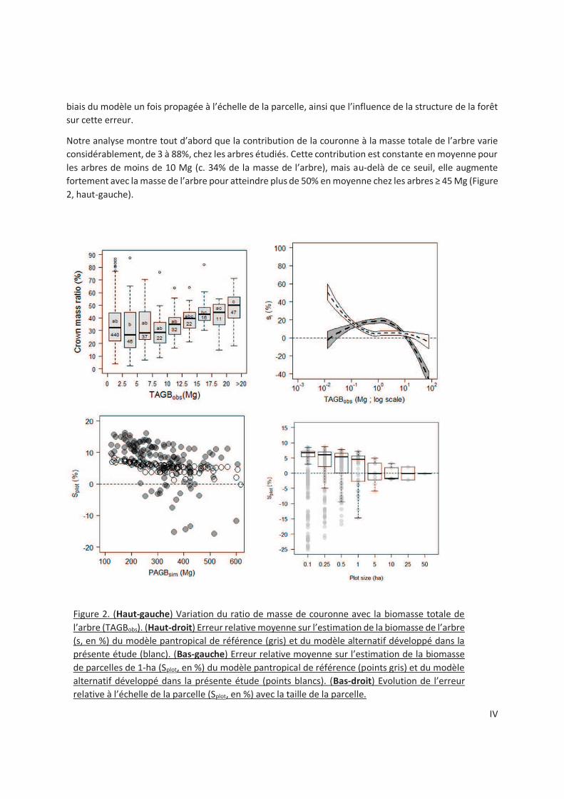
IV
biais du modèle un fois propagée à l’échelle de la parcelle, ainsi que l’influence de la structure de la forêt
sur cette erreur.
Notre analyse montre tout d’abord que la contribution de la couronne à la masse totale de l’arbre varie
considérablement, de 3 à 88%, chez les arbres étudiés. Cette contribution est constante en moyenne pour
les arbres de moins de 10 Mg (c. 34% de la masse de l’arbre), mais au-delà de ce seuil, elle augmente
fortement avec la masse de l’arbre pour atteindre plus de 50% en moyenne chez les arbres ≥ 45 Mg (Figure
2, haut-gauche).
Figure 2. (Haut-gauche) Variation du ratio de masse de couronne avec la biomasse totale de
l’arbre (TAGBobs). (Haut-droit) Erreur relative moyenne sur l’estimation de la biomasse de l’arbre
(s, en %) du modèle pantropical de référence (gris) et du modèle alternatif développé dans la
présente étude (blanc). (Bas-gauche) Erreur relative moyenne sur l’estimation de la biomasse
de parcelles de 1-ha (Splot, en %) du modèle pantropical de référence (points gris) et du modèle
alternatif développé dans la présente étude (points blancs). (Bas-droit) Evolution de l’erreur
relative à l’échelle de la parcelle (Splot, en %) avec la taille de la parcelle.
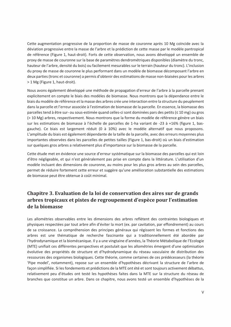
V
Cette augmentation progressive de la proportion de masse de couronne après 10 Mg coïncide avec la
déviation progressive entre la masse de l’arbre et la prédiction de cette masse par le modèle pantropical
de référence (Figure 1, haut-droit). Forts de cette observation, nous avons développé un ensemble de
proxy de masse de couronne sur la base de paramètres dendrométriques disponibles (diamètre du tronc,
hauteur de l’arbre, densité du bois) ou facilement mesurables sur le terrain (hauteur du tronc). L’inclusion
du proxy de masse de couronne le plus performant dans un modèle de biomasse décomposant l’arbre en
deux parties (tronc et couronne) a permis d’obtenir des estimations de masse non-biaisées pour les arbres
> 1 Mg (Figure 1, haut-droit).
Nous avons également développé une méthode de propagation d’erreur de l’arbre à la parcelle prenant
explicitement en compte le biais des modèles de biomasse. Nous montrons que la dépendance entre le
biais du modèle de référence et la masse des arbres crée une interaction entre la structure du peuplement
dans la parcelle et l’erreur associée à l’estimation de biomasse de la parcelle. En essence, la biomasse des
parcelles tend à être sur- ou sous-estimée quand celles-ci sont dominées pars des petits (≤ 10 mg) ou gros
(> 10 Mg) arbres, respectivement. Nous montrons que la forme du modèle de référence génère un biais
sur les estimations de biomasse à l’échelle de parcelles de 1-ha variant de -23 à +16% (figure 1, bas-
gauche). Ce biais est largement réduit (0 à 10%) avec le modèle alternatif que nous proposons.
L’amplitude du biais est également dépendante de la taille de la parcelle, avec des erreurs moyennes plus
importantes observées dans les parcelles de petites tailles (Figure 1, bas-droit) où un biais d’estimation
sur quelques gros arbres a relativement plus d’importance sur la biomasse de la parcelle.
Cette étude met en évidence une source d’erreur systématique sur la biomasse des parcelles qui est loin
d’être négligeable, et qui n’est généralement pas prise en compte dans la littérature. L’utilisation d’un
modèle incluant des dimensions de couronne, au moins pour les plus gros arbres au sein des parcelles,
permet de réduire fortement cette erreur et suggère qu’une amélioration substantielle des estimations
de biomasse peut être obtenue à coût minimal.
Chapitre 3. Evaluation de la loi de conservation des aires sur de grands
arbres tropicaux et pistes de regroupement d’espèce pour l’estimation
de la biomasse
Les allométries observables entre les dimensions des arbres reflètent des contraintes biologiques et
physiques respectées par tout arbre afin d’éviter la mort (ex. par cavitation, par effondrement) au cours
de sa croissance. La compréhension des principes généraux qui régissent les formes et fonctions des
arbres est une thématique de recherche fascinante qui a traditionnellement été abordée par
l’hydrodynamique et la biomécanique. Il y a une vingtaine d’années, la Théorie Métabolique de l’Ecologie
(MTE) unifiait ces différentes perspectives et postulait que les allométries émergent d’une optimisation
évolutive des propriétés de structure et d’hydrodynamique du réseau vasculaire de distribution des
ressources des organismes biologiques. Cette théorie, comme certaines de ces prédécesseurs (la théorie
‘Pipe model’, notamment), repose sur un ensemble d’hypothèses décrivant la structure de l’arbre de
façon simplifiée. Si les fondements et prédictions de la MTE ont été et sont toujours activement débattus,
relativement peu d’études ont testé les hypothèses faites dans la MTE sur la structure du réseau de
branches que constitue un arbre. Dans ce chapitre, nous avons testé un ensemble d’hypothèses de la
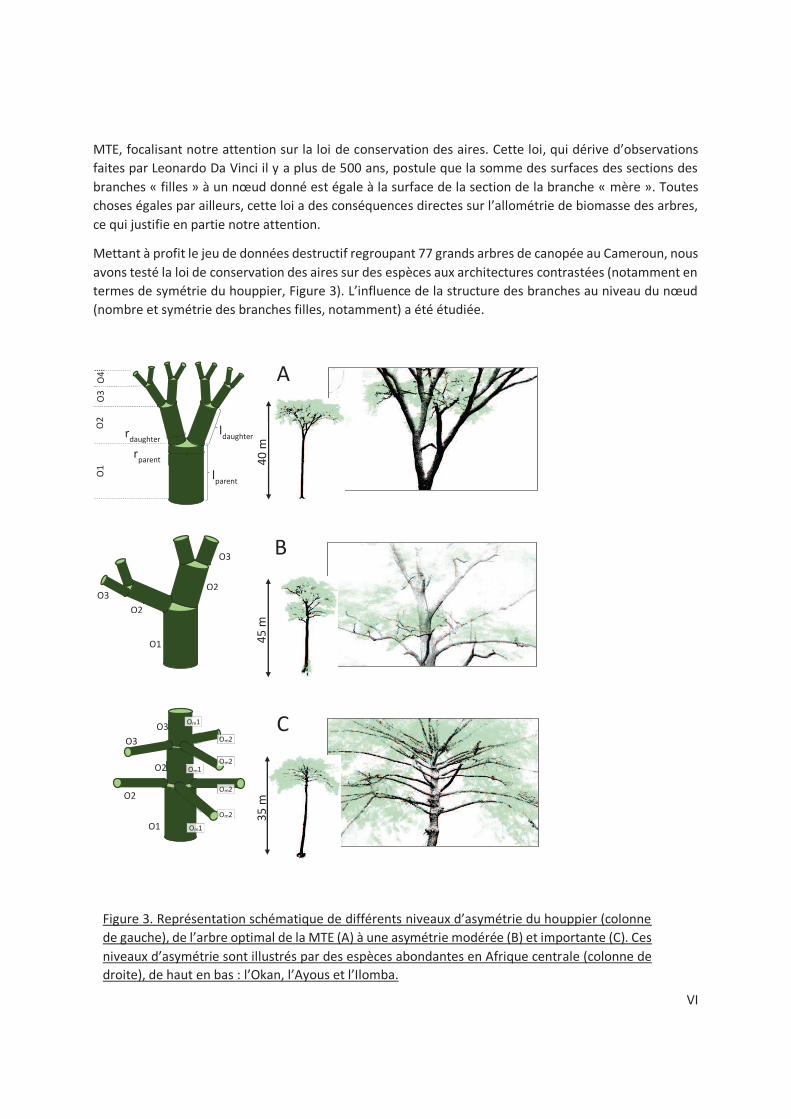
VI
MTE, focalisant notre attention sur la loi de conservation des aires. Cette loi, qui dérive d’observations
faites par Leonardo Da Vinci il y a plus de 500 ans, postule que la somme des surfaces des sections des
branches « filles » à un nœud donné est égale à la surface de la section de la branche « mère ». Toutes
choses égales par ailleurs, cette loi a des conséquences directes sur l’allométrie de biomasse des arbres,
ce qui justifie en partie notre attention.
Mettant à profit le jeu de données destructif regroupant 77 grands arbres de canopée au Cameroun, nous
avons testé la loi de conservation des aires sur des espèces aux architectures contrastées (notamment en
termes de symétrie du houppier, Figure 3). L’influence de la structure des branches au niveau du nœud
(nombre et symétrie des branches filles, notamment) a été étudiée.
40
m
45
m
35
m
lparent
ldaughter
rparent
rdaughter
O1
O2
O3 O
4
O1
O2
A
B
C
O3
O1
O2
O2
O3 O3
O2
O3
Om1
Om1
Om1
Om2
Om2
Om2
Om2
Figure 3. Représentation schématique de différents niveaux d’asymétrie du houppier (colonne
de gauche), de l’arbre optimal de la MTE (A) à une asymétrie modérée (B) et importante (C). Ces
niveaux d’asymétrie sont illustrés par des espèces abondantes en Afrique centrale (colonne de
droite), de haut en bas : l’Okan, l’Ayous et l’Ilomba.
VII
Notre analyse montre que contrairement à la prédiction de la loi de conservation des aires, le ratio des
surfaces des sections des branches filles sur celui de la mère (noté R) est supérieur à 1 en moyenne chez
les grands arbres tropicaux (c. 1.17). Nous avons mis en évidence l’influence systématique de certains
paramètres de structure des couronnes sur R, notamment le nombre de branches filles à un nœud donné
(Figure 4, haut-gauche) et leur symétrie (Figure 4, haut-gauche).
Ces paramètres de structure étant caractéristiques de l’organisation générale des couronnes de certaines
espèces, nous mettons en évidence des variations systématiques de R entre espèces (Figure 4, bas).
Figure 4. (Haut-gauche) Distribution de fréquence des ratios des surfaces des sections des branches filles
sur celles des mères (R) pour des nœuds à 2 filles (gris clair) et pour ceux à plus de 2 filles (gris foncé).
(Haut-droite) Effet de l’asymétrie des filles (noté q) sur R. Les nœuds portant une fille dominante,
verticale, centrale au houppier (notée PA) sont distingués des autres. (Bas-gauche) Somme cumulée des
surfaces des sections des branches filles en fonction de celle de la mère pour l’Ayous et l’Ilomba. La droite
d’ajustement du modèle est représentée en gris foncé. (Bas-droit) Somme cumulée des surfaces des
sections des branches filles en fonction de celle de la mère pour l’Okan. La droite d’ajustement du modèle
est représentée en gris foncé.
L’organisation générale des couronnes reflétant, dans une certaine mesure, la stratégie de vie des
essences (ex. pionnière à croissance rapide vs tolérante à l’ombre à croissance lente), les résultats
donnent lieu à une discussion sur les possibilités de regroupement des espèces dans les modèles de
biomasse.
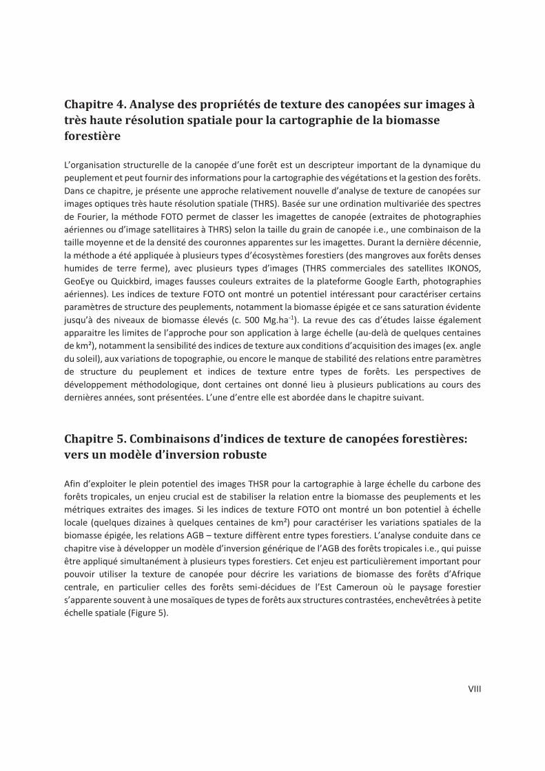
VIII
Chapitre 4. Analyse des propriétés de texture des canopées sur images à
très haute résolution spatiale pour la cartographie de la biomasse
forestière
L’organisation structurelle de la canopée d’une forêt est un descripteur important de la dynamique du
peuplement et peut fournir des informations pour la cartographie des végétations et la gestion des forêts.
Dans ce chapitre, je présente une approche relativement nouvelle d’analyse de texture de canopées sur
images optiques très haute résolution spatiale (THRS). Basée sur une ordination multivariée des spectres
de Fourier, la méthode FOTO permet de classer les imagettes de canopée (extraites de photographies
aériennes ou d’image satellitaires à THRS) selon la taille du grain de canopée i.e., une combinaison de la
taille moyenne et de la densité des couronnes apparentes sur les imagettes. Durant la dernière décennie,
la méthode a été appliquée à plusieurs types d’écosystèmes forestiers (des mangroves aux forêts denses
humides de terre ferme), avec plusieurs types d’images (THRS commerciales des satellites IKONOS,
GeoEye ou Quickbird, images fausses couleurs extraites de la plateforme Google Earth, photographies
aériennes). Les indices de texture FOTO ont montré un potentiel intéressant pour caractériser certains
paramètres de structure des peuplements, notamment la biomasse épigée et ce sans saturation évidente
jusqu’à des niveaux de biomasse élevés (c. 500 Mg.ha-1). La revue des cas d’études laisse également
apparaitre les limites de l’approche pour son application à large échelle (au-delà de quelques centaines
de km²), notamment la sensibilité des indices de texture aux conditions d’acquisition des images (ex. angle
du soleil), aux variations de topographie, ou encore le manque de stabilité des relations entre paramètres
de structure du peuplement et indices de texture entre types de forêts. Les perspectives de
développement méthodologique, dont certaines ont donné lieu à plusieurs publications au cours des
dernières années, sont présentées. L’une d’entre elle est abordée dans le chapitre suivant.
Chapitre 5. Combinaisons d’indices de texture de canopées forestières:
vers un modèle d’inversion robuste
Afin d’exploiter le plein potentiel des images THSR pour la cartographie à large échelle du carbone des
forêts tropicales, un enjeu crucial est de stabiliser la relation entre la biomasse des peuplements et les
métriques extraites des images. Si les indices de texture FOTO ont montré un bon potentiel à échelle
locale (quelques dizaines à quelques centaines de km²) pour caractériser les variations spatiales de la
biomasse épigée, les relations AGB – texture diffèrent entre types forestiers. L’analyse conduite dans ce
chapitre vise à développer un modèle d’inversion générique de l’AGB des forêts tropicales i.e., qui puisse
être appliqué simultanément à plusieurs types forestiers. Cet enjeu est particulièrement important pour
pouvoir utiliser la texture de canopée pour décrire les variations de biomasse des forêts d’Afrique
centrale, en particulier celles des forêts semi-décidues de l’Est Cameroun où le paysage forestier
s’apparente souvent à une mosaïques de types de forêts aux structures contrastées, enchevêtrées à petite
échelle spatiale (Figure 5).
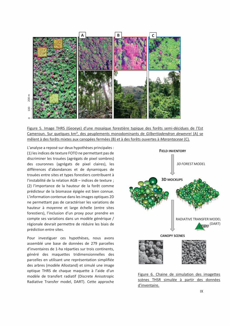
IX
Figure 5. Image THRS (Geoeye) d’une mosaïque forestière typique des forêts semi-décidues de l’Est
Cameroun. Sur quelques km², des peuplements monodominants de Gilbertiodendron dewevrei (A) se
mêlent à des forêts mixtes aux canopées fermées (B) et à des forêts ouvertes à Marantaceae (C).
L’analyse a reposé sur deux hypothèses principales :
(1) les indices de texture FOTO ne permettant pas de
discriminer les trouées (agrégats de pixel sombres)
des couronnes (agrégats de pixel claires), les
différences d’abondances et de dynamiques de
trouées entre sites et types forestiers contribuent à
l’instabilité de la relation AGB – indices de texture ;
(2) l’importance de la hauteur de la forêt comme
prédicteur de la biomasse épigée est bien connue.
L’information contenue dans les images optiques 2D
ne permettant pas de caractériser les variations de
hauteur à moyenne et large échelle (entre sites
forestiers), l’inclusion d’un proxy pour prendre en
compte ses variations dans un modèle générique /
régionale devrait permettre de réduire les biais de
prédiction entre sites.
Pour investiguer ces hypothèses, nous avons
assemblé une base de données de 279 parcelles
d’inventaires de 1-ha réparties sur trois continents,
généré des maquettes tridimensionnelles des
parcelles en utilisant une représentation simplifiée
des arbres (modèle Allostand) et simulé une image
optique THRS de chaque maquette à l’aide d’un
modèle de transfert radiatif (Discrete Anisotropic
Radiative Transfer model, DART). Cette approche
0
10
0
20
0 m
A B C
3D MOCKUPS
CANOPY SCENES
3D FOREST MODEL
RADIATIVE TRANSFER MODEL (DART)
FIELD INVENTORY
Figure 6. Chaine de simulation des imagettes
scènes THSR simulée à partir des données
d’inventaire.
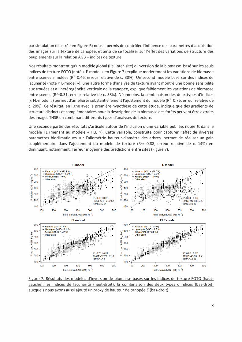
X
par simulation (illustrée en Figure 6) nous a permis de contrôler l’influence des paramètres d’acquisition
des images sur la texture de canopée, et ainsi de se focaliser sur l’effet des variations de structure des
peuplements sur la relation AGB – indices de texture.
Nos résultats montrent qu’un modèle global (i.e. inter-site) d’inversion de la biomasse basé sur les seuls
indices de texture FOTO (noté « F-model » en Figure 7) explique modérément les variations de biomasse
entre scènes simulées (R²=0.46, erreur relative de c. 30%). Un second modèle basé sur des indices de
lacunarité (noté « L-model »), une autre forme d’analyse de texture ayant montré une bonne sensibilité
aux trouées et à l’hétérogénéité verticale de la canopée, explique faiblement les variations de biomasse
entre scènes (R²=0.31, erreur relative de c. 38%). Néanmoins, la combinaison des deux types d’indices
(« FL-model ») permet d’améliorer substantiellement l’ajustement du modèle (R²=0.76, erreur relative de
c. 20%). Ce résultat, en ligne avec la première hypothèse de cette étude, indique que des gradients de
structure distincts et complémentaires pour la description de la biomasse des forêts peuvent être extraits
des images THSR en combinant différents types d’analyses de texture.
Une seconde partie des résultats s’articule autour de l’inclusion d’une variable publiée, notée E, dans le
modèle FL (menant au modèle « FLE »). Cette variable, construite pour capturer l’effet de diverses
paramètres bioclimatiques sur l’allométrie hauteur-diamètre des arbres, permet de réaliser un gain
supplémentaire dans l’ajustement du modèle de texture (R²= 0.88, erreur relative de c. 14%) en
diminuant, notamment, l’erreur moyenne des prédictions entre sites (Figure 7).
Figure 7. Résultats des modèles d’inversion de biomasse basés sur les indices de texture FOTO (haut-
gauche), les indices de lacunarité (haut-droit), la combinaison des deux types d’indices (bas-droit)
auxquels nous avons aussi ajouté un proxy de hauteur de canopée E (bas-droit).
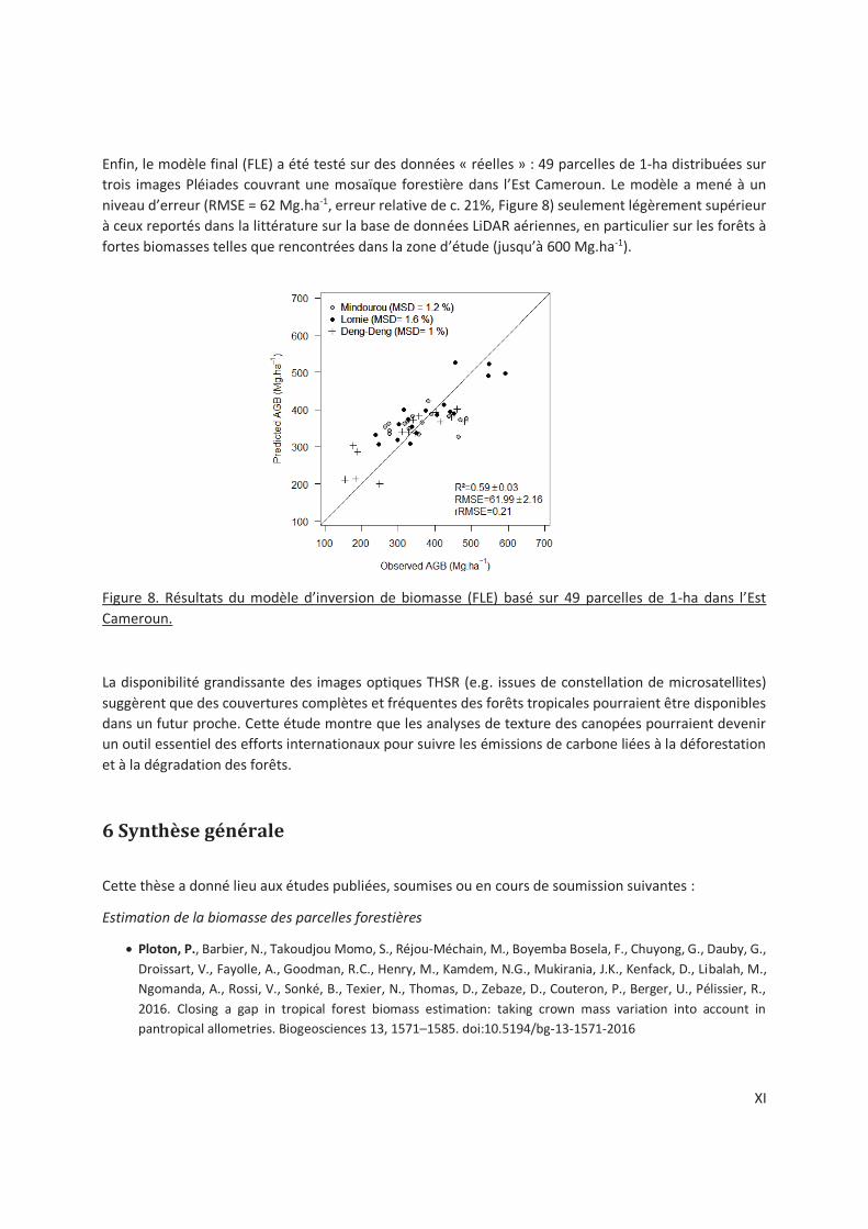
XI
Enfin, le modèle final (FLE) a été testé sur des données « réelles » : 49 parcelles de 1-ha distribuées sur
trois images Pléiades couvrant une mosaïque forestière dans l’Est Cameroun. Le modèle a mené à un
niveau d’erreur (RMSE = 62 Mg.ha-1, erreur relative de c. 21%, Figure 8) seulement légèrement supérieur
à ceux reportés dans la littérature sur la base de données LiDAR aériennes, en particulier sur les forêts à
fortes biomasses telles que rencontrées dans la zone d’étude (jusqu’à 600 Mg.ha-1).
Figure 8. Résultats du modèle d’inversion de biomasse (FLE) basé sur 49 parcelles de 1-ha dans l’Est
Cameroun.
La disponibilité grandissante des images optiques THSR (e.g. issues de constellation de microsatellites)
suggèrent que des couvertures complètes et fréquentes des forêts tropicales pourraient être disponibles
dans un futur proche. Cette étude montre que les analyses de texture des canopées pourraient devenir
un outil essentiel des efforts internationaux pour suivre les émissions de carbone liées à la déforestation
et à la dégradation des forêts.
6 Synthèse générale
Cette thèse a donné lieu aux études publiées, soumises ou en cours de soumission suivantes :
Estimation de la biomasse des parcelles forestières
· Ploton, P., Barbier, N., Takoudjou Momo, S., Réjou-Méchain, M., Boyemba Bosela, F., Chuyong, G., Dauby, G.,
Droissart, V., Fayolle, A., Goodman, R.C., Henry, M., Kamdem, N.G., Mukirania, J.K., Kenfack, D., Libalah, M.,
Ngomanda, A., Rossi, V., Sonké, B., Texier, N., Thomas, D., Zebaze, D., Couteron, P., Berger, U., Pélissier, R.,
2016. Closing a gap in tropical forest biomass estimation: taking crown mass variation into account in
pantropical allometries. Biogeosciences 13, 1571–1585. doi:10.5194/bg-13-1571-2016
XII
· Ploton, P., Barbier, N., Couteron, P., Momo, S.T., Griffon, S., Bonaventure, S., Uta, B., Pélissie,r R. Assessing
Leonardo’s rule on large tropical trees of contrasted architectures. En preparation pour Trees – Structure and
Function.
· Picard, N., Rutishauser, E., Ploton, P., Ngomanda, A., Henry, M., 2015. Should tree biomass allometry be
restricted to power models? For. Ecol. Manag. 353, 156–163. doi:10.1016/j.foreco.2015.05.035
· Chave, J., Réjou-Méchain, M., Búrquez, A., Chidumayo, E., Colgan, M.S., Delitti, W.B.C., Duque, A., Eid, T.,
Fearnside, P.M., Goodman, R.C., Henry, M., Martínez-Yrízar, A., Mugasha, W.A., Muller-Landau, H.C.,
Mencuccini, M., Nelson, B.W., Ngomanda, A., Nogueira, E.M., Ortiz-Malavassi, E., Pélissier, R., Ploton, P., Ryan,
C.M., Saldarriaga, J.G., Vieilledent, G., 2014. Improved allometric models to estimate the aboveground
biomass of tropical trees. Glob. Change Biol. 20, 3177–3190. doi:10.1111/gcb.12629
Lien entre arbres de canopée visibles sur images THRS et biomasse de la forêt
· Bastin, J.-F., Barbier, N., Réjou-Méchain, M., Fayolle, A., Gourlet-Fleury, S., Maniatis, D., de Haulleville, T., Baya,
F., Beeckman, H., Beina, D., Couteron, P., Chuyong, G., Dauby, G., Doucet, J.-L., Droissart, V., Dufrêne, M.,
Ewango, C., Gillet, J.F., Gonmadje, C.H., Hart, T., Kavali, T., Kenfack, D., Libalah, M., Malhi, Y., Makana, J.-R.,
Pélissier, R., Ploton, P., Serckx, A., Sonké, B., Stevart, T., Thomas, D.W., De Cannière, C., Bogaert, J., 2015c.
Seeing Central African forests through their largest trees. Sci. Rep. 5, 13156. doi:10.1038/srep13156
· Blanchard, E., Birnbaum, P., Ibanez, T., Boutreux, T., Antin, C., Ploton, P., Vincent, G., Pouteau, R., Vandrot, H.,
Hequet, V., 2016. Contrasted allometries between stem diameter, crown area, and tree height in five tropical
biogeographic areas. Trees 1–16.
· Jucker, T., Caspersen, J., Chave, J., Antin, C., Barbier, N., Bongers, F., Dalponte, M., van Ewijk, K.Y., Forrester,
D.I., Haeni, M., Higgins, S.I., Holdaway, R.J., Iida, Y., Lorimer, C., Marshall, P.L., Momo, S., Moncrieff, G.R.,
Ploton, P., Poorter, L., Rahman, K.A., Schlund, M., Sonké, B., Sterck, F.J., Trugman, A.T., Usoltsev, V.A.,
Vanderwel, M.C., Waldner, P., Wedeux, B.M.M., Wirth, C., Wöll, H., Woods, M., Xiang, W., Zimmermann, N.E.,
Coomes, D.A., 2016. Allometric equations for integrating remote sensing imagery into forest monitoring
programmes. Glob. Change Biol. doi:10.1111/gcb.13388
Estimation de la biomasse sur base des propriétés de texture des canopées
· Ploton, P., Pélissier, R., Barbier, N., Proisy, C., Ramesh, B.R., Couteron, P., 2013. Canopy texture analysis for
large-scale assessments of tropical forest stand structure and biomass, in: Treetops at Risk. Springer, pp. 237–
245.
· Ploton, P., Barbier, N., Couteron, P., Ayyappan, N., Antin, C.M., Bastin, J.-F., Chuyong, G., Dauby, G., Droissart,
V., Gastellu-Etchegorry, J.-P., Kamdem, N.G., Kenfack, D., Libalah, M., Momo, S., Pargal, S., Proisy, C., Sonké,
B., Texier, N., Thomas, D., Zebaze, D., Verley, P., Vincent, G., Berger, U., Pélissier, R. Combining canopy texture
metrics from optical data to retrieve tropical forest aboveground biomass in complex forest mosaics. En
révision dans Remote Sensing of Environment.
· Ploton, P., Pélissier, R., Proisy, C., Flavenot, T., Barbier, N., Rai, S.N., Couteron, P., 2012. Assessing aboveground
tropical forest biomass using Google Earth canopy images. Ecol. Appl. 22, 993–1003. doi:10.1890/11-1606.1
· Couteron, P., Barbier, N., Deblauwe, V., Pélissier, R., Ploton, P., 2015. Texture Analysis of Very High Spatial
Resolution Optical Images as a Way to Monitor Vegetation and Forest Biomass in the Tropics. Multi-Scale For.
Biomass Assess. Monit. Hindu Kush Himal. Reg. Geospatial Perspect. 157.

Title : Improving tropical forest aboveground biomass estimations : insights from canopy trees structure
and spatial organization
Keywords : forest carbon, REDD, pantropical biomass allometric model, canopy structure, canopy texture,
passive optical imagery, Fourier transform, lacunarity
Abstract : Tropical forests store more than half of the world’s forest carbon and are particularly threatened
by deforestation and degradation processes, which together represent the second largest source of
anthropogenic CO2 emissions. Consequently, tropical forests are the focus of international climate policies
(i.e. Reducing emissions from deforestation and forest degradation, REDD) aiming at reducing forest-
related CO2 emissions. The REDD initiative lies on our ability to map forest carbon stocks (i.e. spatial
dynamics) and to detect deforestation and degradations (i.e. temporal dynamics) at large spatial scales (e.g.
national, forested basin), with accuracy and precision. Remote-sensing is as a key tool for this purpose, but
numerous sources of error along the carbon mapping chain makes meeting REDD criteria an outstanding
challenge. In the present thesis, we assessed carbon (quantified through aboveground biomass, AGB)
estimation error at the tree- and plot-level using a widely used pantropical AGB model, and at the
landscape-level using a remote sensing method based on canopy texture features from very high resolution
(VHR) optical data. Our objective was to better understand and reduce AGB estimation error at each level
using information on large canopy tree structure, distribution and spatial organization.
Although large trees disproportionally contributed to forest carbon stock, they are under-represented in
destructive datasets and subject to an under-estimation bias with the pantropical AGB model. We
destructively sampled 77 very large tropical trees and assembled a large (pantropical) dataset to study how
variation in tree form (through crown sizes and crown mass ratio) contributed to this error pattern. We
showed that the source of bias in the pantropical model was a systematic increase in the proportion of tree
mass allocated to the crown in canopy trees. An alternative AGB model accounting for this phenomenon
was proposed. We also propagated the AGB model bias at the plot-level and showed that the interaction
between forest structure and model bias, although often overlooked, might in fact be substantial. We
further analyzed the structural properties of crown branching networks in light of the assumptions and
predictions of the Metabolic Theory of Ecology, which supports the power-form of the pantropical AGB
model. Important deviations were observed, notably from Leonardo’s rule (i.e. the principle of area
conservation), which, all else being equal, could support the higher proportion of mass in large tree crowns.
A second part of the thesis dealt with the extrapolation of field-plot AGB via canopy texture features of VHR
optical data. A major barrier for the development of a broad-scale forest carbon monitoring method based
on canopy texture is that relationships between canopy texture and stand structure parameters (including
AGB) vary among forest types and regions of the world. We investigated this discrepancy using a simulation
approach: virtual canopy scenes were generated for 279 1-ha plots distributed on contrasted forest types
across the tropics. We showed that complementing FOTO texture with additional descriptors of forest
structure, notably on canopy openness (from a lacunarity analysis) and tree slenderness (from a bioclimatic
proxy) allows developing a stable inversion frame for forest AGB at large scale. Although the approach we
proposed requires further empirical validation, a first case study on a forests mosaic in the Congo basin
gave promising results.
Overall, this work increased our understanding of mechanisms behind AGB estimation errors at the tree-,
plot- and landscape-level. It stresses the need to better account for variation patterns in tree structure (e.g.
ontogenetic pattern of carbon allocation) and forest structural organization (across forest types, under
different environmental conditions) to improve general AGB models, and in fine our ability to accurately
map forest AGB at large scale.
Titre : Amélioration des estimations de biomasse en forêt tropicale : apport de la structure et de
l’organisation spatiale des arbres de canopée
Mots clés : carbone forestier, REDD, modèle de biomasse pantropical, structure de canopée, texture de
canopée, imagerie optique passive, transformée de Fourier, lacunarité
Résumé : Les forêts tropicales séquestrent plus de la moitié du carbone forestier mondial et sont
particulièrement menacées par les processus de déforestation et de dégradation, qui représentent la
deuxième source d’émissions anthropogéniques de CO2. De fait, les forêts tropicales sont au centre de
politiques climatiques internationales (i.e. Reducing emissions from deforestation and forest degradation,
REDD) visant à réduire ces émissions. L’initiative REDD repose sur notre capacité à cartographier les stocks
de carbone forestier (dynamique spatiale) et à détecter la déforestation et la dégradation (dynamique
temporelle) à large échelle spatiale (e.g. nationale, bassin forestier), avec exactitude et précision. Dans ce
cadre, la télédétection apparait comme un outil crucial, mais les nombreuses sources d’erreur dans la
chaîne de cartographie du carbone font des objectifs du REDD un challenge ambitieux. Dans cette thèse,
nous avons évalué les erreurs associées aux estimations de carbone forestier (quantifié au travers de la
biomasse épigée, AGB) (1) aux échelles de l’arbre et du peuplement en utilisant un modèle pantropical
largement employé et (2) à l’échelle du paysage en utilisant une méthode de télédétection basée sur les
caractéristiques texturales d’images optiques à très haute résolution spatiale. Notre objectif général était
de mieux comprendre et de réduire l’erreur d’estimation de l’AGB à chaque échelle par une meilleure prise
en compte de la structure, de la distribution et de l’organisation spatiale des arbres de canopée.
Malgré l’importance des grands arbres dans la dynamique du carbone forestier, ils sont sous-représentés
dans les jeux de données destructifs et soumis à un biais de sous-estimation dans le modèle d’AGB
pantropical. Nous avons assemblé une base de données pantropicale et étudié l’influence de la forme de
l’arbre sur le patron d’erreur du modèle. Nos résultats montrent que la source de biais du modèle est une
augmentation de la masse de l’arbre dans la couronne chez les arbres de canopée. Un modèle d’AGB
prenant ce phénomène en compte a été proposé. Nous avons aussi propagé le biais du modèle à l’échelle
du peuplement et montré que l’interaction entre la structure du peuplement et l’erreur du modèle, qui est
souvent négligée, peut en fait être substantielle. Une analyse des propriétés structurelles des couronnes a
également été menée au regard des hypothèses de la Théorie Métabolique de l’Ecologie Des déviations ont
été observées, notamment à la loi de Léonardo (i.e. principe de conservation des aires), qui, toutes choses
égales par ailleurs, pourraient justifier la grande proportion de masse trouvée dans les couronnes des
arbres de canopée.
Une seconde partie de la thèse porte sur l’extrapolation des estimations d’AGB des parcelles de terrain via
les caractéristiques de texture des canopées extraites par transformée de Fourier (i.e. méthode FOTO). Un
obstacle majeur au développement d’une méthode d’estimation de l’AGB à large échelle basée sur la
texture tient au fait que la relation texture – paramètres de structure du peuplement varie entre types de
forêt et régions du monde. Nous avons investigué cette question en simulant des scènes de canopées
virtuelles pour 279 parcelles de 1 ha établies dans des types de forêts tropicales contrastés. Nous montrons
qu’en complémentant les indices de texture FOTO avec d’autres descripteurs structuraux, notamment sur
l’ouverture de la canopée (via une analyse de lacunarité) et l’élancement des arbres (via un proxy
bioclimatique), il devrait être possible de développer un cadre d’inversion stable de l’AGB à large échelle.
Un premier cas d’étude empirique dans une mosaïque forestière du bassin du Congo a donné des résultats
prometteurs.
Globalement, ce travail met en évidence le besoin de mieux prendre en compte les patrons de variation de
structure de l’arbre (e.g. ontogénétique) et de la forêt afin d’améliorer les modèles génériques d’AGB.