improving u.s. stock return forecasts: a “fair-value” cape ... · nevertheless, with...

1

Improving U.S. stock return forecasts: A “fair-value” CAPE approach Authors1 Joseph H. Davis, Ph.D. Vanguard, Investment Strategy Group Roger Aliaga-Díaz, Ph.D. Vanguard, Investment Strategy Group Harshdeep Ahluwalia, M.Sc. Vanguard, Investment Strategy Group Ravi Tolani Duke University, Fuqua School of Business

July 2017

ABSTRACT

The accuracy of U.S. stock return forecasts based on the cyclically-adjusted P/E (CAPE) ratio

has deteriorated since 1985. The issue is not the CAPE ratio, but CAPE regressions that assume

it reverts mechanically to its long-run average. Our approach conditions mean reversion in the

CAPE ratio on real (not nominal) bond yields, reducing out-of-sample forecast errors by as much

as 50%. At present, low real bond yields imply low real earnings yields and an above-average

“fair-value” CAPE ratio. Nevertheless, with Shiller’s CAPE ratio now well above its fair value,

our model predicts muted U.S. stock returns over the next decade.

Keywords: Stock returns, return predictability, CAPE ratio, real bond yields

1 We wish to acknowledge Jack Bogle, Scott Pappas, Denis Chaves, and Fei Xu for their useful comments to this paper. The views expressed in this working paper do not necessarily reflect the views of The Vanguard Group, Inc.

2

Professors John Campbell and Robert Shiller’s (1988) cyclically-adjusted P/E (or, CAPE) ratio is

arguably the most widely-followed metric in the investment profession to judge whether or not a

stock market is fairly valued. The CAPE ratio’s popularity is due in part to the power of mean

reversion. A high (low) cyclically-adjusted P/E (CAPE) ratio has been associated with below-

average (above-average) 10-year-ahead U.S. stock returns.

Nevertheless, stock return predictions using the Shiller CAPE ratio have generally not performed

well more recently. Beginning around 1985, average out-of-sample forecast errors of the

predicted returns ten years ahead (i.e., 1995 and on) have been larger than if one had used the

trailing historical long-run average. The rise in average forecast error has coincided with the

secular rise in the CAPE ratio above its 1926-1984 average of 14.6. Indeed, the Shiller CAPE

ratio has defied mean reversion since that time, having only once dropped below its long-run

average. And realized U.S. stock returns over the past three decades have been robust,

notwithstanding the global financial crisis.

Even with Shiller’s CAPE ratio above a frothy 29 as of June 30th, 2017, industry experts do not

agree on how much the U.S. stock market is “over-valued.2” Some focus on refining how the

Shiller CAPE ratio is constructed. For instance, Siegel (2016) argues the secular rise in the

CAPE ratio’s trend is due to changes in accounting standards, and that NIPA (national income

and product account) earnings should serve as the “E” in the CAPE ratio. Using a NIPA-based

CAPE ratio, Siegel contends that U.S. stocks are not overvalued.

2 See, for instance, Foster’s (2017) CFA Institute blog at https://blogs.cfainstitute.org/investor/2017/06/13/shiller-vs-siegel-is-the-stock-market-overvalued/

3

The economic environment has also been cited as another factor in (justifying) elevated CAPE

ratios. On a keynote panel at the 70th Annual CFA National Conference in May 2017, Professors

Jeremy Siegel and Robert Shiller both cited low interest rates as a potential factor in the extended

period of elevated CAPE ratios, although neither explicitly quantified the link between interest

rates and future stock returns. This paper does just that.

Here we show that the primary issue is not with the Shiller CAPE ratio. Rather, it’s with simple

regressions that assume the CAPE ratio will revert mechanically to its fixed long-run average,

regardless of the economic environment. We stipulate that the “fair-value” CAPE ratio (i.e., the

value that the actual CAPE ratio should eventually revert to) varies over time, dependent on the

state of the economy, as measured by real interest rates, expected inflation, and measures of

financial volatility. In our framework, lower real bond yields imply lower real earnings yields

and a higher “fair-value” CAPE ratio, all else equal. Real yields matter in our framework, not

nominal yields per se as in the so-called Fed Model (Asness, 2003).

Our methodology is most similar to the pioneering work of Bogle (1991, 1995) and Bogle and

Nolan (2015). The so-called Occam’s razor model of Bogle and Nolan (2015) projects ten-year-

ahead U.S. stock returns based on the current level of the dividend yield, the trailing 10-year-

average in earnings growth, and a straight-lined reversion of the current P/E ratio to its trailing

30-year average. We attempt to maintain the elegant simplicity of Bogle and Nolan’s approach,

while refining and improving upon the assumption of—and economic rationale for—CAPE

mean reversion. Both approaches tend to produce similar stock forecasts unless real bond yields

differ from their long-run average at the time that the stock market forecast is made. That is

4

certainly the case today; as of December 31st, 2016 our derived real ten-year Treasury yield was

near 0%.

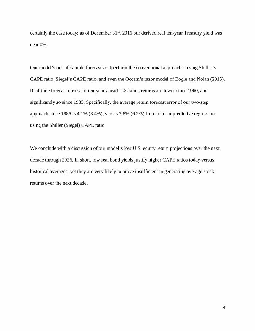
Our model’s out-of-sample forecasts outperform the conventional approaches using Shiller’s

CAPE ratio, Siegel’s CAPE ratio, and even the Occam’s razor model of Bogle and Nolan (2015).

Real-time forecast errors for ten-year-ahead U.S. stock returns are lower since 1960, and

significantly so since 1985. Specifically, the average return forecast error of our two-step

approach since 1985 is 4.1% (3.4%), versus 7.8% (6.2%) from a linear predictive regression

using the Shiller (Siegel) CAPE ratio.

We conclude with a discussion of our model’s low U.S. equity return projections over the next

decade through 2026. In short, low real bond yields justify higher CAPE ratios today versus

historical averages, yet they are very likely to prove insufficient in generating average stock

returns over the next decade.

5

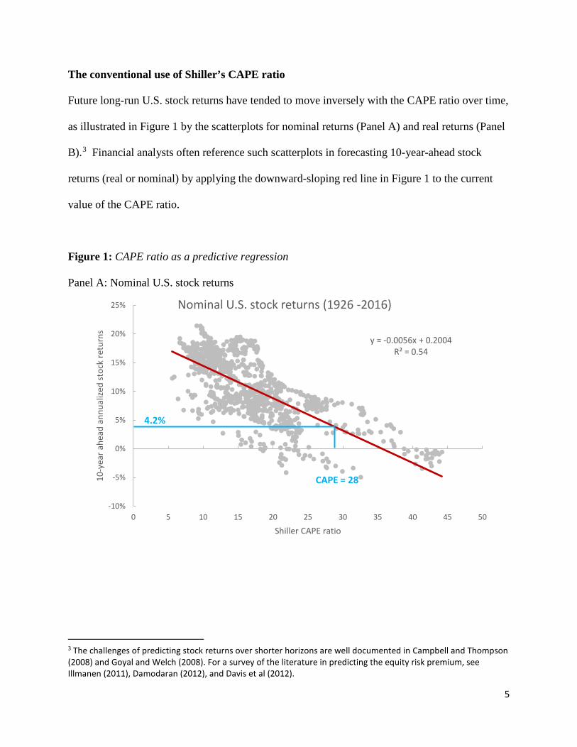
The conventional use of Shiller’s CAPE ratio

Future long-run U.S. stock returns have tended to move inversely with the CAPE ratio over time,

as illustrated in Figure 1 by the scatterplots for nominal returns (Panel A) and real returns (Panel

B).3 Financial analysts often reference such scatterplots in forecasting 10-year-ahead stock

returns (real or nominal) by applying the downward-sloping red line in Figure 1 to the current

value of the CAPE ratio.

Figure 1: CAPE ratio as a predictive regression Panel A: Nominal U.S. stock returns

3 The challenges of predicting stock returns over shorter horizons are well documented in Campbell and Thompson (2008) and Goyal and Welch (2008). For a survey of the literature in predicting the equity risk premium, see Illmanen (2011), Damodaran (2012), and Davis et al (2012).

y = -0.0056x + 0.2004R² = 0.54

-10%

-5%

0%

5%

10%

15%

20%

25%

0 5 10 15 20 25 30 35 40 45 50

10-y

ear a

head

ann

ualiz

ed st

ock

retu

rns

Shiller CAPE ratio

Nominal U.S. stock returns (1926 -2016)

CAPE = 28

4.2%

6

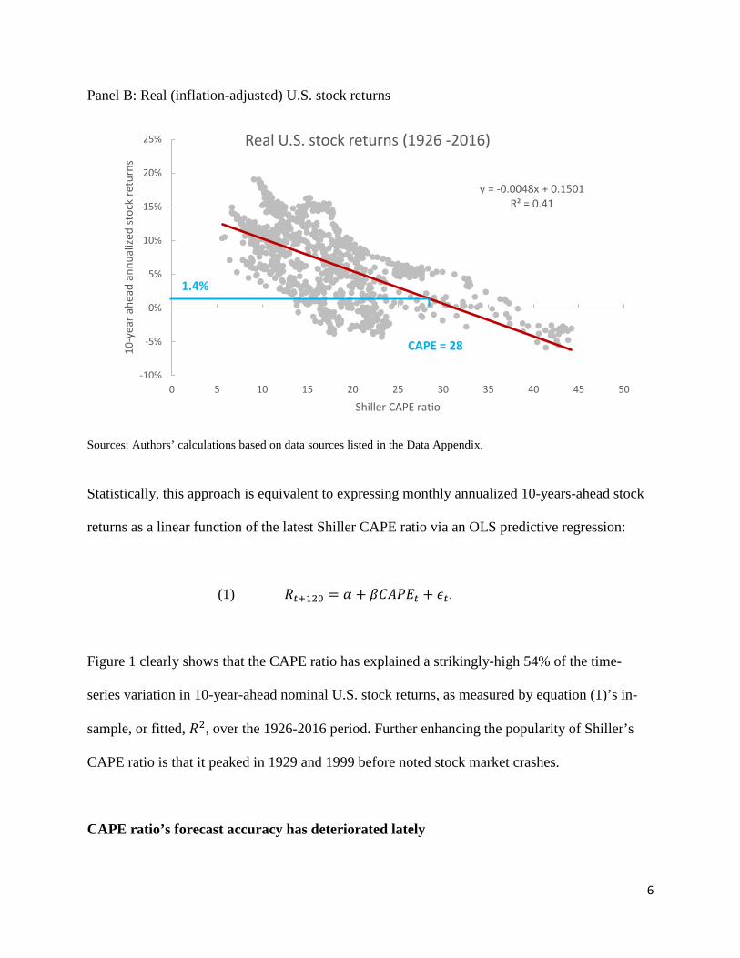
Panel B: Real (inflation-adjusted) U.S. stock returns

Sources: Authors’ calculations based on data sources listed in the Data Appendix.

Statistically, this approach is equivalent to expressing monthly annualized 10-years-ahead stock

returns as a linear function of the latest Shiller CAPE ratio via an OLS predictive regression:

(1) 𝑅𝑅𝑡𝑡+120 = 𝛼𝛼 + 𝛽𝛽𝐶𝐶𝐶𝐶𝐶𝐶𝐶𝐶𝑡𝑡 + 𝜖𝜖𝑡𝑡.

Figure 1 clearly shows that the CAPE ratio has explained a strikingly-high 54% of the time-

series variation in 10-year-ahead nominal U.S. stock returns, as measured by equation (1)’s in-

sample, or fitted, 𝑅𝑅2, over the 1926-2016 period. Further enhancing the popularity of Shiller’s

CAPE ratio is that it peaked in 1929 and 1999 before noted stock market crashes.

CAPE ratio’s forecast accuracy has deteriorated lately

y = -0.0048x + 0.1501R² = 0.41

-10%

-5%

0%

5%

10%

15%

20%

25%

0 5 10 15 20 25 30 35 40 45 50

10-y

ear a

head

ann

ualiz

ed st

ock

retu

rns

Shiller CAPE ratio

Real U.S. stock returns (1926 -2016)

CAPE = 28

1.4%

7

Unfortunately, CAPE ratio’s out-of-sample forecast accuracy has weakened since the mid-1980s

versus its in-sample fit, as illustrated in Table 1. To be sure, the correlations between actual U.S.

stock returns and those predicted ten years prior by the Shiller CAPE ratio have remained high in

real time. Since 1960, the correlation has been 83%, and a remarkable 91% since 1985. But there

is an important catch.

Table 1: The CAPE ratio’s predictive power out-of-sample Panel A: Nominal returns

Panel B: Real returns

Notes: The statistics shown are for 10-year annualized returns using the traditional predictive regression equation (1) with Shiller CAPE and Siegel CAPE. A “*” next to the RMSE refers to the significance of the Diebold-Mariano test (2002) of whether the forecast is statically better or worse than the historical mean. Significance level at 90%, 95% and 99% are denoted by one, two and three asterisks respectively. Sources: Authors’ calculations.

We must stress that correlation is not necessarily a reliable indicator of forecast accuracy.

Correlation of predicted

returns with actual

Average forecast error

(RMSE)

Model forecast error relative to error of using a

naïve historical mean forecast


returns with actual

Average forecast error (RMSE)



Historical average 5.8% 6.2%

Shiller CAPE ratio 83% 5.5%* LOWER 91% 7.8%*** HIGHER

Siegel CAPE ratio 67% 4.9%*** LOWER 90% 6.2% SIMILAR

Out-of-sample forecasts made since 1985

Predictive variable



returns with actual


(RMSE)




returns with actual





Shiller CAPE ratio 56% 6.3% SIMILAR 81% 7.8%*** HIGHER

Siegel CAPE ratio 36% 6.2% SIMILAR 76% 5.8% SIMILAR


Predictive variable


8

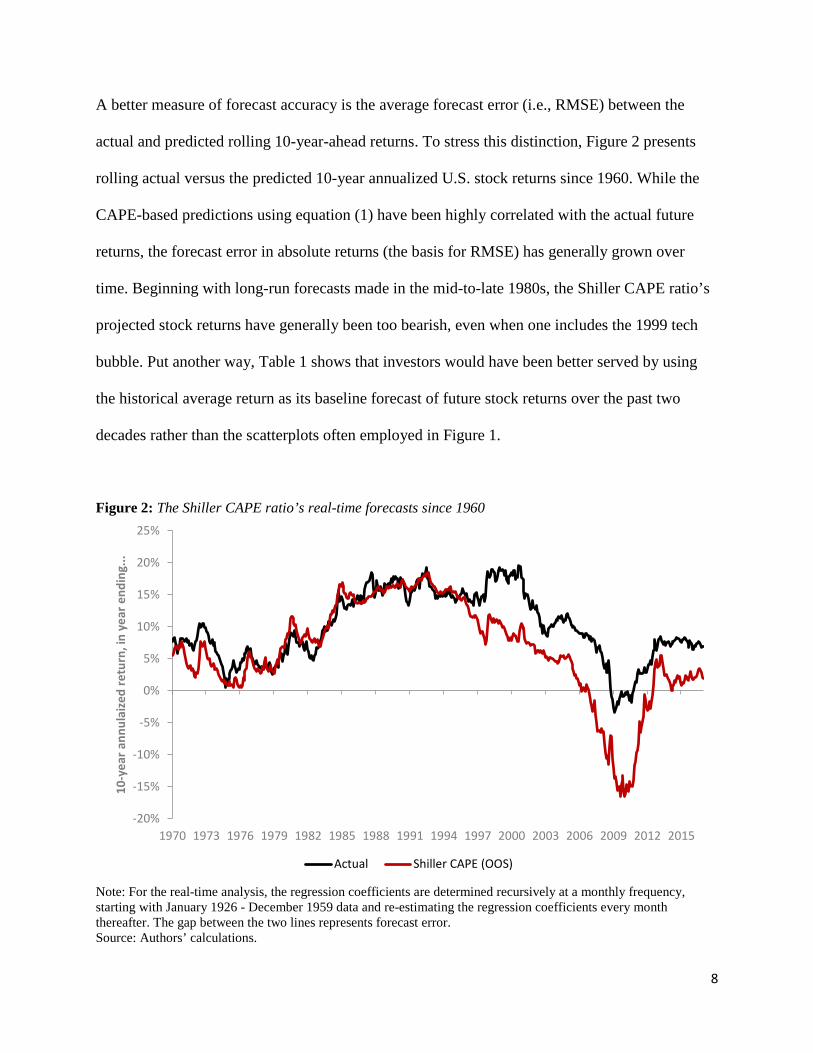
A better measure of forecast accuracy is the average forecast error (i.e., RMSE) between the

actual and predicted rolling 10-year-ahead returns. To stress this distinction, Figure 2 presents

rolling actual versus the predicted 10-year annualized U.S. stock returns since 1960. While the

CAPE-based predictions using equation (1) have been highly correlated with the actual future

returns, the forecast error in absolute returns (the basis for RMSE) has generally grown over

time. Beginning with long-run forecasts made in the mid-to-late 1980s, the Shiller CAPE ratio’s

projected stock returns have generally been too bearish, even when one includes the 1999 tech

bubble. Put another way, Table 1 shows that investors would have been better served by using

the historical average return as its baseline forecast of future stock returns over the past two

decades rather than the scatterplots often employed in Figure 1.

Figure 2: The Shiller CAPE ratio’s real-time forecasts since 1960

Note: For the real-time analysis, the regression coefficients are determined recursively at a monthly frequency, starting with January 1926 - December 1959 data and re-estimating the regression coefficients every month thereafter. The gap between the two lines represents forecast error. Source: Authors’ calculations.

-20%

-15%

-10%

-5%

0%

5%

10%

15%

20%

25%

1970 1973 1976 1979 1982 1985 1988 1991 1994 1997 2000 2003 2006 2009 2012 2015

10-y

ear a

nnul

aize

d re

turn

, in

year

end

ing.

..

Actual Shiller CAPE (OOS)

9

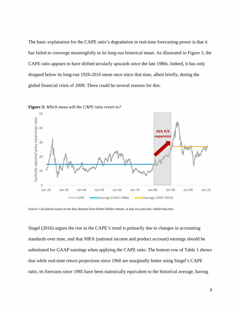
The basic explanation for the CAPE ratio’s degradation in real-time forecasting power is that it

has failed to converge meaningfully to its long-run historical mean. As illustrated in Figure 3, the

CAPE ratio appears to have drifted secularly upwards since the late 1980s. Indeed, it has only

dropped below its long-run 1926-2016 mean once since that time, albeit briefly, during the

global financial crisis of 2009. There could be several reasons for this.

Figure 3: Which mean will the CAPE ratio revert to?

Source: Calculations based on the data obtained from Robert Shiller website, at aida.wss.yale.edu/~shiller/data.htm.

Siegel (2016) argues the rise in the CAPE’s trend is primarily due to changes in accounting

standards over time, and that NIPA (national income and product account) earnings should be

substituted for GAAP earnings when applying the CAPE ratio. The bottom row of Table 1 shows

that while real-time return projections since 1960 are marginally better using Siegel’s CAPE

ratio, its forecasts since 1985 have been statistically equivalent to the historical average, having

0

10

20

30

40

50

Jan-26 Jan-36 Jan-46 Jan-56 Jan-66 Jan-76 Jan-86 Jan-96 Jan-06 Jan-16

Cycl

ical

ly a

djus

ted

pric

e to

earn

ings

ratio

CAPE Average (1926-1986) Average (1997-2016)

95% P/E expansion

10

roughly the same RMSE. Regardless of how we define or smooth earnings here, the real-time

forecasting accuracy has been weaker than its in-sample fit. Changing the definition of “E” in the

CAPE ratio has apparently not been a panacea for forecasting U.S. stock returns.

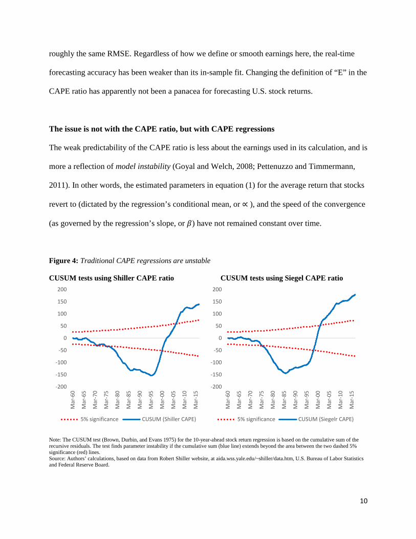
The issue is not with the CAPE ratio, but with CAPE regressions

The weak predictability of the CAPE ratio is less about the earnings used in its calculation, and is

more a reflection of model instability (Goyal and Welch, 2008; Pettenuzzo and Timmermann,

2011). In other words, the estimated parameters in equation (1) for the average return that stocks

revert to (dictated by the regression’s conditional mean, or ∝ ), and the speed of the convergence

(as governed by the regression’s slope, or 𝛽𝛽) have not remained constant over time.

Figure 4: Traditional CAPE regressions are unstable CUSUM tests using Shiller CAPE ratio CUSUM tests using Siegel CAPE ratio

Note: The CUSUM test (Brown, Durbin, and Evans 1975) for the 10-year-ahead stock return regression is based on the cumulative sum of the recursive residuals. The test finds parameter instability if the cumulative sum (blue line) extends beyond the area between the two dashed 5% significance (red) lines. Source: Authors’ calculations, based on data from Robert Shiller website, at aida.wss.yale.edu/~shiller/data.htm, U.S. Bureau of Labor Statistics and Federal Reserve Board.

-200

-150

-100

-50

0

50

100

150

200

Mar

-60

Mar

-65

Mar

-70

Mar

-75

Mar

-80

Mar

-85

Mar

-90

Mar

-95

Mar

-00

Mar

-05

Mar

-10

Mar

-15

5% significance CUSUM (Shiller CAPE)

-200

-150

-100

-50

0

50

100

150

200

Mar

-60

Mar

-65

Mar

-70

Mar

-75

Mar

-80

Mar

-85

Mar

-90

Mar

-95

Mar

-00

Mar

-05

Mar

-10

Mar

-15

5% significance CUSUM (Siegelr CAPE)

11

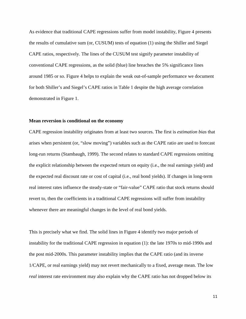
As evidence that traditional CAPE regressions suffer from model instability, Figure 4 presents

the results of cumulative sum (or, CUSUM) tests of equation (1) using the Shiller and Siegel

CAPE ratios, respectively. The lines of the CUSUM test signify parameter instability of

conventional CAPE regressions, as the solid (blue) line breaches the 5% significance lines

around 1985 or so. Figure 4 helps to explain the weak out-of-sample performance we document

for both Shiller’s and Siegel’s CAPE ratios in Table 1 despite the high average correlation

demonstrated in Figure 1.

Mean reversion is conditional on the economy

CAPE regression instability originates from at least two sources. The first is estimation bias that

arises when persistent (or, “slow moving”) variables such as the CAPE ratio are used to forecast

long-run returns (Stambaugh, 1999). The second relates to standard CAPE regressions omitting

the explicit relationship between the expected return on equity (i.e., the real earnings yield) and

the expected real discount rate or cost of capital (i.e., real bond yields). If changes in long-term

real interest rates influence the steady-state or “fair-value” CAPE ratio that stock returns should

revert to, then the coefficients in a traditional CAPE regressions will suffer from instability

whenever there are meaningful changes in the level of real bond yields.

This is precisely what we find. The solid lines in Figure 4 identify two major periods of

instability for the traditional CAPE regression in equation (1): the late 1970s to mid-1990s and

the post mid-2000s. This parameter instability implies that the CAPE ratio (and its inverse

1/CAPE, or real earnings yield) may not revert mechanically to a fixed, average mean. The low

real interest rate environment may also explain why the CAPE ratio has not dropped below its

12

long-run average of 16.9 since 1990, albeit for a brief time during the global financial crisis of

2009. The parameter instability in the CAPE regression appear to coincide with material shifts in

average real bond yields, such as the high average real yields between the late 1970s and mid-

1990s, and the secularly lower real yields before and after that period.

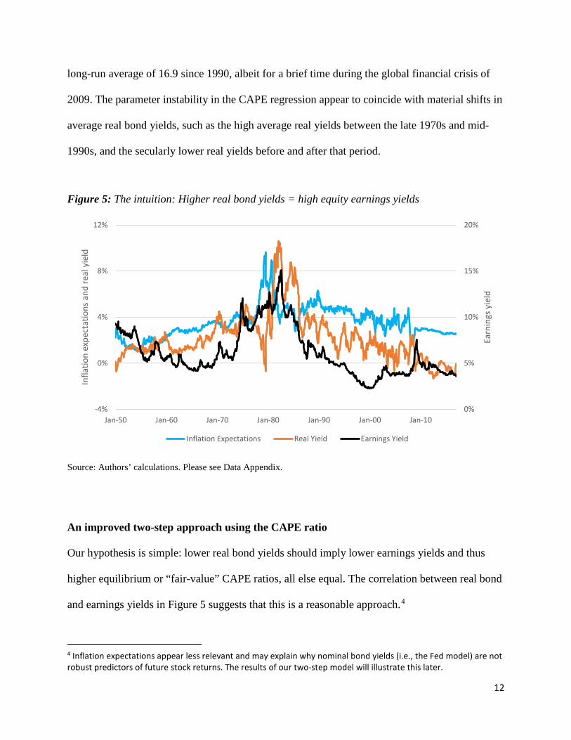
Figure 5: The intuition: Higher real bond yields = high equity earnings yields

Source: Authors’ calculations. Please see Data Appendix.

An improved two-step approach using the CAPE ratio

Our hypothesis is simple: lower real bond yields should imply lower earnings yields and thus

higher equilibrium or “fair-value” CAPE ratios, all else equal. The correlation between real bond

and earnings yields in Figure 5 suggests that this is a reasonable approach.4

4 Inflation expectations appear less relevant and may explain why nominal bond yields (i.e., the Fed model) are not robust predictors of future stock returns. The results of our two-step model will illustrate this later.

0%

5%

10%

15%

20%

-4%

0%

4%

8%

12%

Jan-50 Jan-60 Jan-70 Jan-80 Jan-90 Jan-00 Jan-10

Earn

ings

yie

ld

Infla

tion

expe

ctat

ions

and

real

yie

ld

Inflation Expectations Real Yield Earnings Yield

13

Motivated by this insight, we propose a simple, two-step approach to forecast stock returns.

While our model differs from the approach typically taken in equation (1), it can be estimated in

real-time using standard software, it does not involve “look-ahead bias,” and, for the U.S. stock

market, it only requires the variables in the CAPE ratio data file conveniently provide by

Professor Robert Shiller’s website.

Our methodology is most similar to the original work of Bogle (1991, 1995) and Bogle and

Nolan (2015). The so-called Occam’s razor model of Bogle and Nolan (2015) projects ten-year-

ahead U.S. stock returns based on the current level of the dividend yield, the trailing 10-year-

average in earnings growth, and a straight-lined reversion of the current P/E ratio to its trailing

30-year average. We attempt to maintain the elegant simplicity of Bogle and Nolan’s approach,

while refining and improving upon the assumption of—and economic rationale for—CAPE

mean reversion. Both approaches should produce similar stock forecasts unless real bond yields

differ from their long-run average at the time that the stock market forecast is made.

Step 1: A VAR model with earnings yields, 1 𝐶𝐶𝐶𝐶𝐶𝐶𝐶𝐶⁄

Unlike traditional methods, we do not forecast returns directly, but rather forecast the inverse of

the CAPE ratio itself. Specifically, we estimate a vector autoregressive (VAR) model with

twelve monthly lags of the form:

(2) Xt = α + β1Xt−1 + β2Xt−2 + ⋯+ β12Xt−12 + εt,

where 𝑿𝑿𝑡𝑡 is a vector of the five variables in the VAR model in logarithmic form, including:

• CAPE real earnings yield, or 1 𝐶𝐶𝐶𝐶𝐶𝐶𝐶𝐶⁄

14

• Real 10-year bond yields, or nominal Treasury yield less an estimated 10-year expected

inflation rate (see Appendix)

• Year-over-year CPI inflation rate

• Realized S&P500 price volatility, over trailing 12 months, and

• Realized volatility of changes in our real bond yield series, over trailing 12 months.5

The motivation of including these five VAR variables derives from Asness (2003), who finds

that earnings yield rises when bond yields rise, when stock volatility rises, and when bond

market volatility falls. Note that we lag the “E” in the CAPE ratio by six months and the CPI

data two months to account for real-time data availability at any month end.

Step 2: Impute stock returns from the CAPE earnings yield forecasts

Rather than estimating equation (1), we calculate future returns directly based on their three

components, thereby reducing estimation bias. We adapt the framework of Bogle and Nolan

(2015) and Ferreira and Santa-Clara (2011) in imputing monthly stock returns by their “sum of

parts” identity:

(3) rt+1 ≡ %∆PEt+1 + %∆Et+1 + DPt+1

where %∆PE is the percentage change in P/E ratio, %∆E is earnings growth, and DP is the

dividend yield. The VAR model’s forecast for the earnings yield provides us the percentage

changes in CAPE ratios, %∆PEt+1, for imputing stock returns directly by the “sum of parts” 5 The motivation of including these five VAR variables derives from Asness (2003), who finds that earnings yield rises when bond yields rise, when stock volatility rises, and when bond market volatility falls. Arnott, Chaves, and Chow (2015) find that both real yields and inflation expectations are positively related to the earnings yield on U.S. stocks. It remains unclear why inflation expectations – a component of nominal bond yields – should influence earnings yields since stocks are a long-run inflation hedge (Illmanen, 2011, ch. 8). Importantly, this so-called “inflation illusion” effect is weaker in our VAR model than the effect from real bond yields given the joint dynamics of our VAR model, which we discuss below.

15

equation (3). For simplicity, we assume that earnings growth is constant and equal to its long-

term average, while the dividend yield is the product of the earnings yield times the payout

ratio.6 As a result, only earnings yield (1 𝐶𝐶𝐶𝐶𝐶𝐶𝐶𝐶⁄ ) has to be forecasted via regression in order to

predict stock returns at a given horizon. At any point in time, the VAR can forecast out for ten

years the CAPE earnings yield and, via step 2, derive an expected future 10-year-ahead return on

U.S. stocks. Table 2 summarizes the similarities and differences between our approach compared

to (a) traditional Shiller CAPE regressions / scatterplots, and (b) the Bogle Occam’s razor model.

Table 2: Comparison of different stock forecasting approaches

Sources: Authors’ calculations.

The potential benefit of our approach is that the “fair-value” CAPE ratio—which the actual

CAPE ratio should revert back to—is permitted to vary over time conditional on the movements 6 The benefit of our “sum of parts” approach is that it should mitigate so-called Stambaugh (1999) bias that can plague predictive regressions with persistent regressors like CAPE ratios that involve overlapping data (Nelson and Kim, 1993). In results unreported here but available upon request, including changes in earnings growth in the VAR does not materially alter the results. Consistent with Cochrane (2008), changes in earnings yields help predict future stock returns, not earnings growth.

Traditional Shiller CAPE ratio regression Bogle Occam's razor model This paper's two-step approach

Dividend yieldSwept into OLS alpha / intercept

coefficient Actual value at beginning of periodDerived from forecasted earnings

yield (below) times the beginning of period payout ratio

Earnings growth Swept into OLS alpha / intercept coefficient

Uses trailing 10-year earnings growth Uses trailing long-run historical average earnings growth

CAPE ratio "mean reversion" process

Estimated by "beta" of the regression; not conditional on any

other variables

Linear proration over ten years between last available PE ratio and trailing 30-year average; provides

"speculative return"; not conditional on any other variables

Forecased earnings yield from 5-variable VAR model that also

includes real bond yields, inflation, real bond volatility and equity

volatility

Stock return component

Ingredients in the stock-return forecasts

16

in these other fundamental variables.7 It is this “fair-value” CAPE that should be the relevant

benchmark for forecasting the equity risk premium, not the CAPE long-run average.8 Put another

way, if actual CAPE ratios revert back to our fair-value CAPE ratio and not CAPE’s historical

average, then our two-step model should produce more reliable stock return forecasts than

traditional Shiller CAPE regressions.

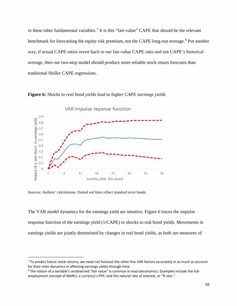
Figure 6: Shocks to real bond yields lead to higher CAPE earnings yields

Sources: Authors’ calculations. Dotted red lines reflect standard error bands.

The VAR model dynamics for the earnings yield are intuitive. Figure 6 traces the impulse

response function of the earnings yield (1/CAPE) to shocks to real bond yields. Movements in

earnings yields are jointly determined by changes in real bond yields, as both are measures of

7 To predict future stock returns, we need not forecast the other five VAR factors accurately in as much as account for their inter-dynamics in affecting earnings yields through time. 8 The notion of a variable’s unobserved “fair value” is common in macroeconomics. Examples include the full-employment concept of NAIRU, a currency’s PPP, and the natural rate of interest, or “R-star.”

17

expected future economic growth and monetary policy.9 The intuition for the positive correlation

between real bond yields and stock earnings yield is simple; lower expected economic growth

implies lower real bond yields, which implies lower earnings yield on stocks, and thus a higher

“fair value” CAPE ratio, all else equal. The disinflationary period and bond-bull market of the

1980s coincided with rising stock valuations. As real interest rates fell below their historical

averages in the 1990s and 2000s, equity earnings yield remained below their own average levels,

too.

Comparing real-time forecasts: An illustration

Figure 7 compares the projections for the earnings yield (1/CAPE) from two models: (a) that

which is implied by a traditional Shiller CAPE regression10, and (2) our VAR model. For

convenience, we re-express the earnings yield as the CAPE ratio. We choose December, 1999,

when the CAPE was above 40, to illustrate relative forecast performance.

Following the dot-com bust period after 1999, the VAR-based CAPE projections anticipate

subsequent CAPE trends more accurately than even equation (1). This is because earnings yields

are not assumed to converge unconditionally to their long-run average as typical Shiller CAPE

regressions do, but rather are a function of the current state of other variables in the model.

Rising real bond yields—combined with the CAPE ratio above its fair value—leads to a sharper 9 Historically, earnings yield and real bond yields have tended to move in tandem. We also know that “breaks” in real yields and inflation expectations occurred during the early 1950s (the end of the Treasury-Fed accord that pegged interest rates after WWII), the mid-1970s (the OPEC oil shock) and the early 1980s (when Volcker and the Fed tamped down higher inflation) given changes in macroeconomic regimes. In results unreported here, we link the structural breaks in Shiller CAPE regressions to breaks in real interest rates and other financial conditions which, when controlled for, lead to improved model stability. That is, the VAR equation for the earnings yield does not suffer from structural breaks in either its conditional mean (alpha) or the speed of mean reversion (beta) when the other variables of our VAR model are included. 10 It can be shown that any predictive regression is equivalent to a single-period stock return equation plus an AR(1) or first-order regressive process in the predictor.

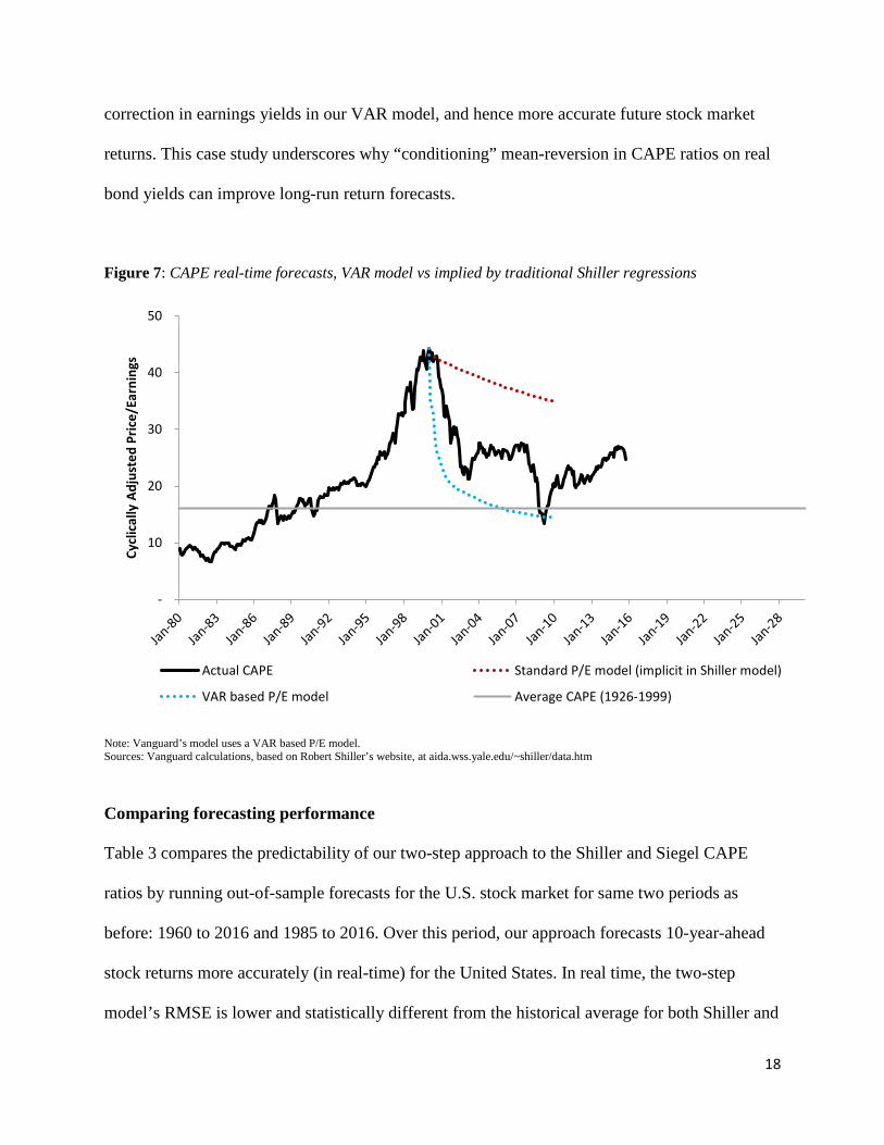
18

correction in earnings yields in our VAR model, and hence more accurate future stock market

returns. This case study underscores why “conditioning” mean-reversion in CAPE ratios on real

bond yields can improve long-run return forecasts.

Figure 7: CAPE real-time forecasts, VAR model vs implied by traditional Shiller regressions

Note: Vanguard’s model uses a VAR based P/E model. Sources: Vanguard calculations, based on Robert Shiller’s website, at aida.wss.yale.edu/~shiller/data.htm Comparing forecasting performance

Table 3 compares the predictability of our two-step approach to the Shiller and Siegel CAPE

ratios by running out-of-sample forecasts for the U.S. stock market for same two periods as

before: 1960 to 2016 and 1985 to 2016. Over this period, our approach forecasts 10-year-ahead

stock returns more accurately (in real-time) for the United States. In real time, the two-step

model’s RMSE is lower and statistically different from the historical average for both Shiller and

-

10

20

30

40

50

Cycl

ical

ly A

djus

ted

Pric

e/Ea

rnin

gs

Actual CAPE Standard P/E model (implicit in Shiller model)

VAR based P/E model Average CAPE (1926-1999)

19

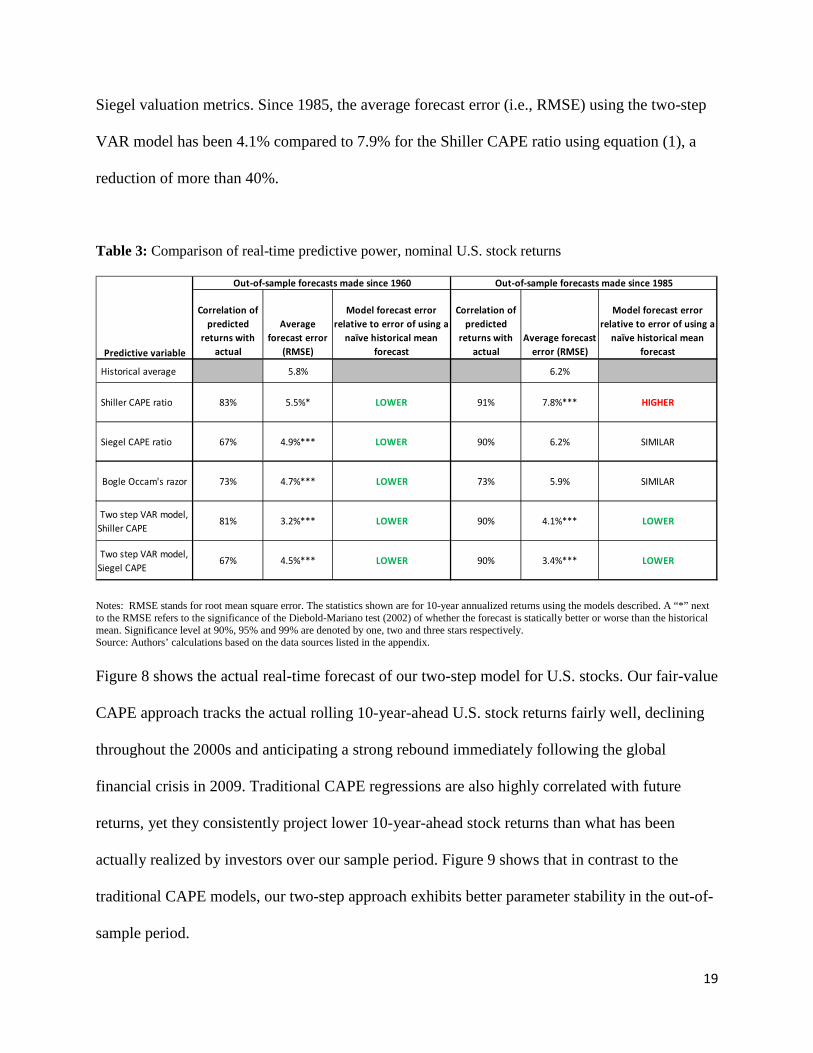
Siegel valuation metrics. Since 1985, the average forecast error (i.e., RMSE) using the two-step

VAR model has been 4.1% compared to 7.9% for the Shiller CAPE ratio using equation (1), a

reduction of more than 40%.

Table 3: Comparison of real-time predictive power, nominal U.S. stock returns

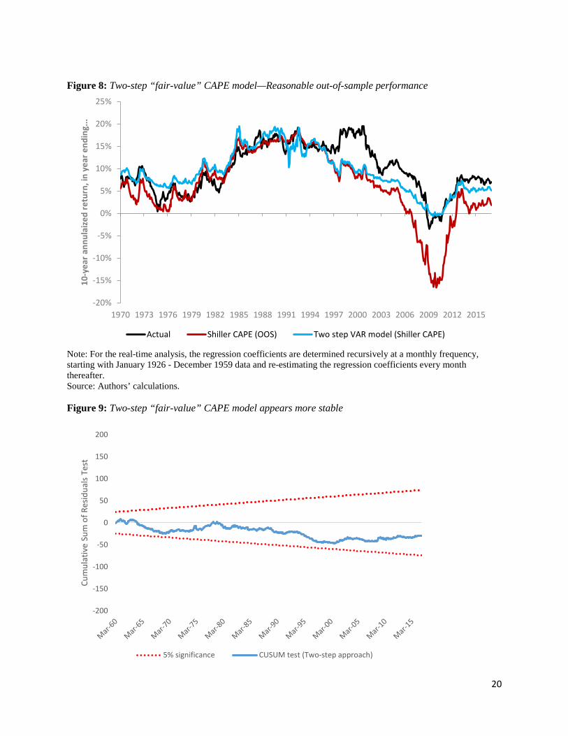
Notes: RMSE stands for root mean square error. The statistics shown are for 10-year annualized returns using the models described. A “*” next to the RMSE refers to the significance of the Diebold-Mariano test (2002) of whether the forecast is statically better or worse than the historical mean. Significance level at 90%, 95% and 99% are denoted by one, two and three stars respectively. Source: Authors’ calculations based on the data sources listed in the appendix. Figure 8 shows the actual real-time forecast of our two-step model for U.S. stocks. Our fair-value

CAPE approach tracks the actual rolling 10-year-ahead U.S. stock returns fairly well, declining

throughout the 2000s and anticipating a strong rebound immediately following the global

financial crisis in 2009. Traditional CAPE regressions are also highly correlated with future

returns, yet they consistently project lower 10-year-ahead stock returns than what has been

actually realized by investors over our sample period. Figure 9 shows that in contrast to the

traditional CAPE models, our two-step approach exhibits better parameter stability in the out-of-

sample period.


returns with actual


(RMSE)




returns with actual





Shiller CAPE ratio 83% 5.5%* LOWER 91% 7.8%*** HIGHER

Siegel CAPE ratio 67% 4.9%*** LOWER 90% 6.2% SIMILAR

Bogle Occam's razor 73% 4.7%*** LOWER 73% 5.9% SIMILAR

Two step VAR model, Shiller CAPE

81% 3.2%*** LOWER 90% 4.1%*** LOWER

Two step VAR model, Siegel CAPE

67% 4.5%*** LOWER 90% 3.4%*** LOWER


Predictive variable


20

Figure 8: Two-step “fair-value” CAPE model—Reasonable out-of-sample performance

Note: For the real-time analysis, the regression coefficients are determined recursively at a monthly frequency, starting with January 1926 - December 1959 data and re-estimating the regression coefficients every month thereafter. Source: Authors’ calculations. Figure 9: Two-step “fair-value” CAPE model appears more stable

-20%

-15%

-10%

-5%

0%

5%

10%

15%

20%

25%

1970 1973 1976 1979 1982 1985 1988 1991 1994 1997 2000 2003 2006 2009 2012 2015

10-y

ear a

nnul

aize

d re

turn

, in

year

end

ing.

..

Actual Shiller CAPE (OOS) Two step VAR model (Shiller CAPE)

-200

-150

-100

-50

0

50

100

150

200

Cum

ulat

ive

Sum

of R

esid

uals

Test

5% significance CUSUM test (Two-step approach)

21

Conclusion

Valuation metrics such as price-earnings ratios are widely followed by the investment

community because they are believed to predict future long-term stock returns. Arguably the

most popular is Robert Shiller’s cyclically-adjusted P/E ratio (or CAPE) which is currently

above its long-run average. However, the out-of-sample forecast accuracy of stock forecasts

produced by CAPE ratios has become increasingly poor. In this paper we have shown why and

offer a solution to offer a more robust approach to produce long-run stock return forecasts.

The problem is not with the CAPE ratio, but with CAPE regressions. We show that a common

industry approach of forecasting long-run stock returns can produce large errors in forecasted

returns due to both estimation bias and its strict assumption that the CAPE ratio will revert over

time to its long-run (and constant) mean. Although far from perfect, our model’s out-of-sample

forecasts for ten-year-ahead U.S. stock returns since 1960 are roughly 40-50% more accurate

than conventional methods. Real-time forecast differences in 10-year-ahead stock returns are

statistically significant, and have grown to exceed three percentage points after 1985 given the

secular decline in real bond yields. In our model, lower real bond yields imply higher

equilibrium CAPE ratios. This framework would appear to explain both elevated CAPE ratios

and robust stock returns over the past two decades. Future research could involve testing our

approach to non-U.S. markets with long-spanning data, or even sectors of the U.S. equity market.

Overall, we encourage investment professionals to adopt our straightforward framework when

forecasting stock returns for strategic asset allocation. Our fair-value approach can be estimated

in real-time using standard software, it does not involve “look-ahead bias,” and, for the U.S.

22

stock market, it only requires the variables in the CAPE ratio data file conveniently provide by

Professor Robert Shiller’s website. As of June 2017, our model projects a guarded, lower-than-

historical return on U.S. stocks of approximately 4.9% over the coming decade. This muted

forecast for U.S. stock returns is not simply because the CAPE ratio is above its long-run mean.

23

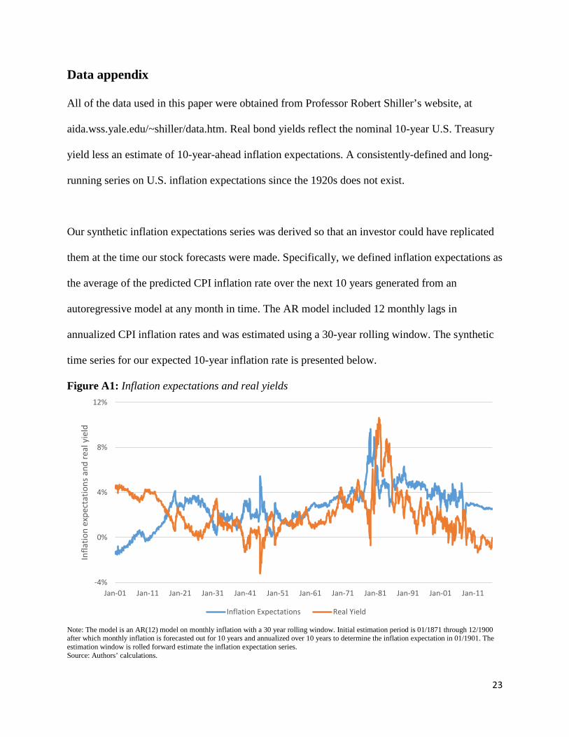
Data appendix All of the data used in this paper were obtained from Professor Robert Shiller’s website, at

aida.wss.yale.edu/~shiller/data.htm. Real bond yields reflect the nominal 10-year U.S. Treasury

yield less an estimate of 10-year-ahead inflation expectations. A consistently-defined and long-

running series on U.S. inflation expectations since the 1920s does not exist.

Our synthetic inflation expectations series was derived so that an investor could have replicated

them at the time our stock forecasts were made. Specifically, we defined inflation expectations as

the average of the predicted CPI inflation rate over the next 10 years generated from an

autoregressive model at any month in time. The AR model included 12 monthly lags in

annualized CPI inflation rates and was estimated using a 30-year rolling window. The synthetic

time series for our expected 10-year inflation rate is presented below.

Figure A1: Inflation expectations and real yields

Note: The model is an AR(12) model on monthly inflation with a 30 year rolling window. Initial estimation period is 01/1871 through 12/1900 after which monthly inflation is forecasted out for 10 years and annualized over 10 years to determine the inflation expectation in 01/1901. The estimation window is rolled forward estimate the inflation expectation series. Source: Authors’ calculations.

-4%

0%

4%

8%

12%

Jan-01 Jan-11 Jan-21 Jan-31 Jan-41 Jan-51 Jan-61 Jan-71 Jan-81 Jan-91 Jan-01 Jan-11

Infla

tion

expe

ctat

ions

and

real

yie

ld

Inflation Expectations Real Yield

24

References

Arnott, Robert D., Denis B. Chaves and Tzee-man Chow. 2015. “King of the Mountain: Shiller

P/E and Macroeconomic Conditions.” Available at

https://papers.ssrn.com/sol3/papers.cfm?abstract_id=2640327, accessed in April, 2017.

Asness, Clifford S. 2000. “Stocks versus Bonds: Explaining the Equity Risk Premium.”

Financial Analysts Journal, vol. 56, no. 2: 96–113.

——. 2003. “Fight the Fed Model.” Journal of Portfolio Management, vol. 30, no. 1: 11–24.

Bogle, John C. 1991. “Investing in the 1990s: Occam’s Razor Revisited.” Journal of Portfolio

Management, vol. 18, no. 1: 88–91.

——. 1995. “The 1990s at the Halfway Mark.” Journal of Portfolio Management, vol. 21, no. 4:

21-31.

Bogle, John C. and Michael W. Nolan, Jr. 2015. “Occam’s Razor Redux: Establishing

Reasonable Expectations for Financial Market Returns.” Journal of Portfolio Management, vol.

42, no. 1 (Fall).

Brown, Robert L., James Durbin, and James M. Evans. 1975. “Techniques for Testing the

Constancy of Regression Relationships over Time.” Journal of the Royal Statistical Society,

Series B (Methodological), vol. 37, no. 2: 149-192.

Campbell, John Y. and Robert J. Shiller. 1988. “Stock Prices, Earnings, and Expected

Dividends.” Journal of Finance, vol. 43, no. 3: 661–676.

——. 1998. “Valuation Ratios and the Long-Run Stock Market Outlook.” Journal of Portfolio

Management, vol. 24, no. 2: 11–26.

Campbell, John Y. and Tuomo Vuolteenaho. 2004. “Inflation Illusion and Stock Prices.”

American Economic Review, vol. 24, no. 2: 11–26.

Campbell, John Y. and Samuel B. Thompson. 2008. “Predicting Excess Stock Returns Out of

Sample: Can Anything Beat the Historical Average? Review of Financial Studies, vol. 21, no. 4:

1509-1531.

https://papers.ssrn.com/sol3/papers.cfm?abstract_id=2640327

25

Cochrane, John H. 2008. “The Dog that Did Not Bark: A Defense of Return Predictability.”

Review of Financial Studies, vol. 21, no. 4: 1533-1575.

——. 2011. “Discount Rates.” The Journal of Finance, vol. 66:, no. 4: 1047-1108.

Damodaran, Aswath. 2012. Equity Risk Premiums (ERP): Determinants, Estimation and

Implications. Available at http://ssrn.com/abstract=2027211, accessed in January, 2017.

Davis, Joseph H., Roger Aliaga-Diaz, and Charles J. Thomas. 2012. “Forecasting Stock Returns:

What Signals Matter, and What Do They Say Now?” Vanguard White Paper.

Diebold, Francis X., and Robert S. Mariano. 2002. “Comparing Predictive Accuracy.” Journal

of Business and Economic Statistics, vol. 20, no. 1: 134-144.

Ferreira, Miguel, A. and Pedro Santa-Clara. 2011. “Forecasting Stock Market Returns: The Sum

of the Parts is More than the Whole.” Journal of Financial Economics, vol. 100, no. 3: 514–537.

Goyal, Amit, and Ivo Welch. 2008. “A Comprehensive Look at the Empirical Performance of

Equity Premium Prediction.” Review of Financial Studies, vol. 21, no. 4: 1455-1508.

Ilmanen, Antti. 2011. Expected Returns: An Investor’s Guide to Harvesting Market Rewards.

West Sussex, United Kingdom: John Wiley & Sons.

Nelson, Charles R., and Myung J. Kim. 1993. “Predictable Stock Returns: The Role of Small

Sample Bias.” Journal of Finance, vol. 48, no. 2: 641-661.

Shiller, Robert. 2000. Irrational Exuberance. Princeton, NJ: Princeton University Press.

Siegel, Jeremy J. 2016. “The Shiller CAPE Ratio: A New Look.” Financial Analysts Journal,

vol. 72, no. 3: 41–50.

Stambaugh, Robert F. 1999. “Predictive Regressions.” Journal of Financial Econometrics, vol.

54: no. 3: 375- 421.

http://ssrn.com/abstract=2027211

improving u.s. stock return forecasts: a “fair-value” cape ... · nevertheless, with...

Documents