improving weather and load forecasting for the …cirrus.ucsd.edu/~pierce/calenergy/deliv3.pdf ·...
TRANSCRIPT
Improving Weather and Load Forecasting
For The California Independent System Operator (CAL ISO): Case Study 1 –
Improving the Forecast of Delta Breeze and Determining The Economic Value
(Deliverable Three)
A Project Sponsored By the National Oceanographic and Atmospheric
Administration (NOAA)
March 12, 2004
Deliverable 3: Improving the Cal ISO Weather and Load Forecast
Scripps Institute of Oceanography (SIO) and Science Applications International Corporation (SAIC) 2
Table of Contents Topic Page No. Contributors and Acknowledgements 3
1. Introduction
A. Background. . . . . . . . . . . . . . . . . . . . . . . . . . . . . . . . . . . . . . . . . . 4
B. The May 28th Event . . . . . . . . . . . . . . . . . . . . . . . . . . . . . . . . . . . 7
C. The Delta Breeze Phenomenon. . . . . . . . . . . . . . . . . . . . . . . . . . 10
D. Cal ISO Needs Assessment. . . . . . . . . . . . . . . . . . . . . . . . . . . . . 12
E. Proposed Case Study. . . . . . . . . . . . . . . . . . . . . . . . . . . . . . . . . . . 17
2. Project Objectives, Literature Search and Approach
A. Objectives of Case Study. . . . . . . . . . . . . . . . . . . . . . . . . . . . . . . 19
B. Summary of Approach. . . . . . . . . . . . . . . . . . . . . . . . . . . . . . . . 19
C. The Cal ISO Review of the Delta Breeze Phenomenon. . . . . 19
D. Literature Review of Delta Breeze. . . . . . . . . . . . . . . . . . . . . . 21
E. Conclusions. . . . . . . . . . . . . . . . . . . . . . . . . . . . . . . . . . . . . . . . . 27
3. Analysis of Delta Breeze Causes, Measurement and Forecasting Issues
A. Background. . . . . . . . . . . . . . . . . . . . . . . . . . . . . . . . . . . . . . . . . . 29
B. Scripps Institution of Oceanography Exploratory Investigation
Into Delta Breeze Dynamics. . . . . . . . . . . . . . . . . . . . . . . . . . . . 29
C. Analysis Approach. . . . . . . . . . . . . . . . . . . . . . . . . . . . . . . . . . . . 31
D. Statistical Analysis and Findings. . . . . . . . . . . . . . . . . . . . . . . . 44
E. Conclusions. . . . . . . . . . . . . . . . . . . . . . . . . . . . . . . . . . . . . . . . . . 51
4. Estimation of the Economic Value of Improved Forecasting of the Delta Breeze For the Cal ISO
A. Objectives. . . . . . . . . . . . . . . . . . . . . . . . . . . . . . . . . . . . . . . . . . . 52
B. Approach. . . . . . . . . . . . . . . . . . . . . . . . . . . . . . . . . . . . . . . . . . . . 54
C. Economic Value of Improved Estimation of Delta Breeze For the Cal ISO. . . . . . . . . . . . . . . . . . . . . . . . . . . 54
D. The Role of Ensemble Forecasts . . . . . . . . . . . . . . . . . . . . . . . .. 63
5. Conclusions
A. Overview. . . . . . . . . . . . . . . . . . . . . . . . . . . . . . . . . . . . . . . . . . . . . 65
B. Key Findings. . . . . . . . . . . . . . . . . . . . . . . . . . . . . . . . . . . . . . . . . 65
C. Implications. . . . . . . . . . . . . . . . . . . . . . . . . . . . . . . . . . . . . . . . . . 66
Appendices
Deliverable 3: Improving the Cal ISO Weather and Load Forecast
Scripps Institute of Oceanography (SIO) and Science Applications International Corporation (SAIC) 3
Contributors and Acknowledgements
This report is sponsored by the National Oceanographic and Atmospheric Administration (NOAA) under contract no.: Key contributors to the report include: Scripps Institution of Oceanography
• Dr. Tim Barnett • Dr. David Pierce • Dr. Anne Steinnemann
Science Applications International Corporation
• Dr. Mary G. Altalo • Mr. Todd D. Davis • Dr. Lorna Greening • Ms. Monica Hale
California Independent System Operator
• Mr. Dennis Gaushel The authors deeply appreciate the support, cooperation and contributions of the California ISO and the National Oceanographic and Atmospheric Administration (NOAA).
Deliverable 3: Improving the Cal ISO Weather and Load Forecast
Scripps Institute of Oceanography (SIO) and Science Applications International Corporation (SAIC) 4
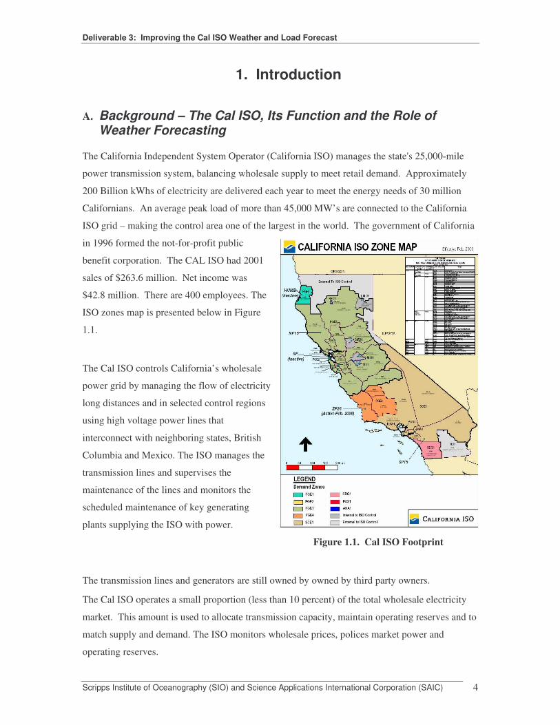
1. Introduction A. Background – The Cal ISO, Its Function and the Role of
Weather Forecasting The California Independent System Operator (California ISO) manages the state's 25,000-mile
power transmission system, balancing wholesale supply to meet retail demand. Approximately
200 Billion kWhs of electricity are delivered each year to meet the energy needs of 30 million
Californians. An average peak load of more than 45,000 MW’s are connected to the California
ISO grid – making the control area one of the largest in the world. The government of California
in 1996 formed the not-for-profit public
benefit corporation. The CAL ISO had 2001
sales of $263.6 million. Net income was
$42.8 million. There are 400 employees. The
ISO zones map is presented below in Figure
1.1.
The Cal ISO controls California’s wholesale
power grid by managing the flow of electricity
long distances and in selected control regions
using high voltage power lines that
interconnect with neighboring states, British
Columbia and Mexico. The ISO manages the
transmission lines and supervises the
maintenance of the lines and monitors the
scheduled maintenance of key generating
plants supplying the ISO with power.
Figure 1.1. Cal ISO Footprint
The transmission lines and generators are still owned by owned by third party owners.
The Cal ISO operates a small proportion (less than 10 percent) of the total wholesale electricity
market. This amount is used to allocate transmission capacity, maintain operating reserves and to
match supply and demand. The ISO monitors wholesale prices, polices market power and
operating reserves.
Deliverable 3: Improving the Cal ISO Weather and Load Forecast
Scripps Institute of Oceanography (SIO) and Science Applications International Corporation (SAIC) 5
The major objectives of the Cal ISO are to:
• Provide open and nondiscriminatory transmission service
• Ensure safe and reliable operation of the grid
• Operate energy and reliability markets in a responsive, flexible and transparent manner
• Foster reasonable energy costs for California consumers.
The Cal ISO operates the transmission grid by completing the following steps:
1. Forecasting power requirements. The Cal ISO publishes a load forecast 24 hours a in
advance and then refines the forecast leading up to two hours before the actual load
occurs.
2. The ISO acts as an electronic auction house coordinating approximately 40,000
transactions for electricity every hour between buyers and sellers, tracking sales and
running complex settlement systems.
3. Schedules for electricity delivery are submitted to the ISO the day before power is
needed.
4. The Cal ISO then runs the schedules through computer systems to mitigate or manage
congestion and account for reserves necessary to plan for contingencies when and if
unexpected events occur – which could be a generating plant outage or a line failure or
over loading.
5. The Cal ISO measures the pulse of the power grid every four seconds to ensure that there
is enough power flowing to meet demand.
6. A controller of 20 transmission paths in the state acts as a controller or gatekeeper to
determine how much power can flow at all of the import/export points.
7. If the Cal ISO sees the demand for power rising higher than expected, it can add
additional power from plants located within and outside the state to meet this growing
requirement. However, this last minute acquisition and scheduling can generally be more
costly than planning for it farther in advance.
8. Power is dispatched from generating units that have been bid into the ISO using
electronic auctions, which automatically set a market-clearing price aimed at creating
reasonable wholesale costs.
Deliverable 3: Improving the Cal ISO Weather and Load Forecast
Scripps Institute of Oceanography (SIO) and Science Applications International Corporation (SAIC) 6
The scheduling coordinators link the ISO, retailers and consumers. They submit schedules to
deliver electricity that meets customer demand with supply. To manage congestion, the ISO runs
the schedules through a program that determines the chance of a power flow “traffic jam” and
then tries to either sell or buy more power with the ISO choosing the least costly method.
There are also electronic auctions for “ancillary services” that are held in the day-ahead and hour
ahead market. This is how the scheduling coordinators submit bids for back up power that the
ISO uses to provide operating reserves to ensure grid reliability.
Hour-ahead schedules are submitted two hours ahead prior to the beginning of the operating
schedule. The scheduling coordinators do not have an opportunity to revise these schedules.
By 10:00 AM the scheduling coordinators submit to the ISO an estimate of how much power they
think their customers will need for the next day and what power plants will produce that energy.
Ancillary bids are accepted for the ISO to procure needed operating reserves.
At 11:00 AM the ISO is ready to give the scheduling coordinators the signal to either proceed
with their schedules for the next day or to modify them. Preliminary ancillary service schedules
are also produced at this time.
By noon the scheduling coordinators must submit revised schedules for the next day. Additional
adjustments might be made to the day -ahead schedules based on other schedules.
By 1:00 PM the ISO closes the day-ahead market and the charge or cost of using the congested
lines is calculated and finalized. Then the ancillary services procurement is published.
As can be seen in this process, for a 24-hour ahead period, monitoring weather and its impact on
load is extremely critical to this process. While the Cal ISO tries to forecast weather in order to
“balance” and optimize grid performance, weather is a “tipping point” that can move the
balancing target. This may also affect the cost of power, congestion and reliability.

Deliverable 3: Improving the Cal ISO Weather and Load Forecast
Scripps Institute of Oceanography (SIO) and Science Applications International Corporation (SAIC) 7
The California ISO region is influenced by a unique summer weather phenomenon generally
referred to as the “Delta Breeze.” This complex weather event has a wide range of impacts on the
Cal ISO system. A strong Delta Breeze, which is associated with wind speeds in the Carquinez
straits of 12 knots or more, ventilates California’s central valley with cool marine air. As a result,
electric loads (driven largely by air conditioning) are substantially lower than if the breeze were
not blowing. If the breeze is not anticipated (or lack thereof), forecast temperatures will be higher
than actually occur, and there are chances that the Cal ISO can over commit to generation supply.
On the other hand, if a Delta Breeze is forecast but none develops, then Cal ISO might under
commit to generating supply – thereby potentially causing threats to reliability, which can be very
costly.
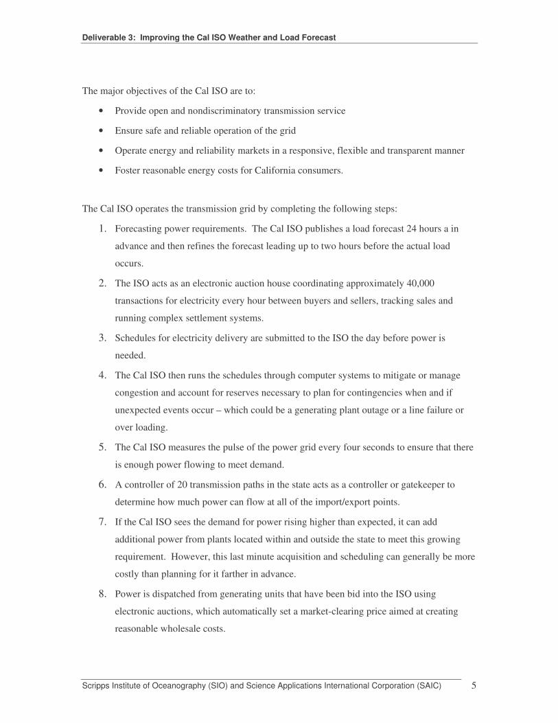
The Cal ISO has found in prior research that peak load increases due to temperature are not linear
in its operating system. Nevertheless, the average change in load with temperature changes is
about 550MW for each degree F increase above 75 F. These rates are different for each of four
major utility operating areas:
• Southern California Edison (SCE) 380 MW/10
• San Diego Gas and Electric (SDG&E) 25 MW/10
• Pacific Gas and Electric (PG&E) Bay Area 80 MW/10
• PG&E Non-Bay Area 210 MW/10.
A graphical display of the daily peak load forecast for weekdays appears in Figure 1.2. The
graph clearly depicts the curvilinear pattern of temperature effects on the load forecast.
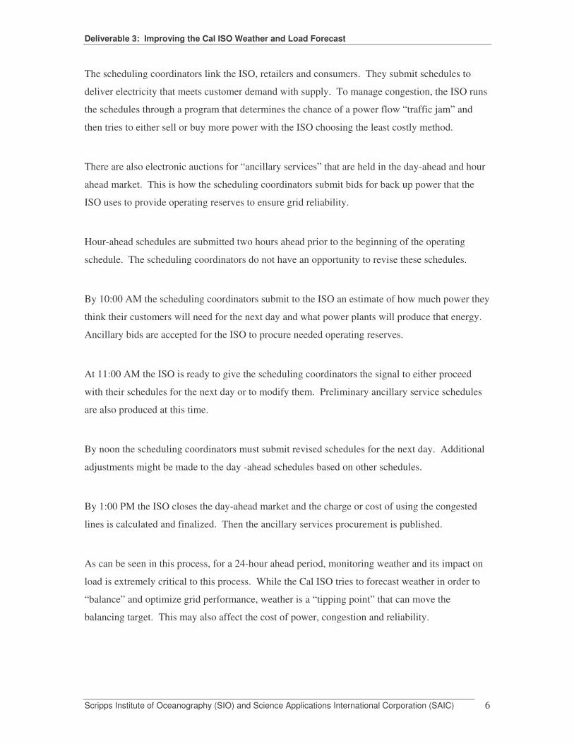
B. The May 28, 2003 Event: A Severe Under-forecast of Peak Load
On May 28, 2003, at approximately 7AM, a routine review of the forecast for the day showed that
the forecast was too low. At 9 AM the peak day forecast was adjusted up. At 3 PM a Stage 1
alert was declared as operating reserved declined below minimum operating levels. At 3:53 PM
the peak load of the day was recorded. Figure 1.3 shows the trend from the initially predicted to
the actual peak of the day. Figure 1.4 shows the hourly changes and the gap of 4,724 MW from
the initial bid load of 34,853 MW to the actual load of 39,577 MW – a gap of 4,724 MW (also
Deliverable 3: Improving the Cal ISO Weather and Load Forecast
Scripps Institute of Oceanography (SIO) and Science Applications International Corporation (SAIC) 8
attribute this figure). This situation is an example of the severity of the problem that can happen
to the Cal ISO when a severe uner-forecast can occur.
Source: http://www.caiso.com/docs/09003a6080/22/c9/09003a608022c993.pdf Figure 1.2. Curvilinear Weather and Load Relationships
Source: http://www.caiso.com/docs/09003a6080/22/c9/09003a608022c993.pdf Figure 1.3. Cal ISO Peak Load Forecast Problems (May 28, 2003)

Deliverable 3: Improving the Cal ISO Weather and Load Forecast
Scripps Institute of Oceanography (SIO) and Science Applications International Corporation (SAIC) 9
“Yes, the winds are quite pronounced and blow in nearly the same direction and magnitude in that area when the Delta Breeze is in effect. These winds carry the cool air from the ocean and cool the entire Central Valley 10-20 degrees and lower the electric load substantially. “ Cal ISO Quote.
Figure 1.4. Illustrative Under-forecast Gap
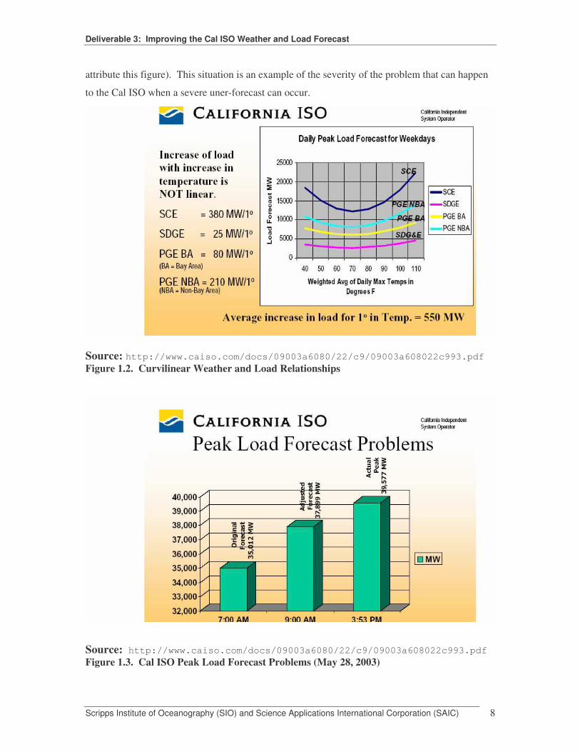
Figures 1.5 and 1.6 show observed versus model predicted (one day in advance) maximum daily
temperature for the Bay area and non-Bay Area (NBA). The predicted values are from the
NOAA AVN MOS forecast, and are a weighted average of the stations Cal ISO has determined to
be the best predictors of electrical load. It can be easily seen that the weighted AVN prediction
has systematic errors. In particular, it does not capture the magnitude of the temperature peaks in
either the Bay or non-Bay Area. Less easy to see is that the larger occurrence of smaller errors,
when weighted by the economic cost of those smaller errors and summed over a year, can be
about equal to the cost of the few large error days. It is these errors that are of great concern to
the Cal ISO. Our analysis of the Cal ISO’s data suggests that commercial weather service
providers often carry these errors in their own forecast.
Deliverable 3: Improving the Cal ISO Weather and Load Forecast
Scripps Institute of Oceanography (SIO) and Science Applications International Corporation (SAIC) 10
C. The Delta Breeze Phenomenon
Since early 2003, the CAL ISO disaggregated their day-ahead load-forecasting model for
Northern California into two areas: the Bay and the non-Bay. A major source of forecast error in
the non-Bay area model is the Delta Breeze condition. Although a maximum daily error series for
forecasts from the non-Bay area model is available from May 18, 2003, through October 14,
2003, no formal error analysis has been completed to identify the causes of this error.
Figure 1.5 AVN Forecast Error for the Bay Area
Figure 1.6 AVN Forecast Error for the Non-Bay Area
Bay Area Observed T vs. AVN Forecast T
65
7075
80
85
9095
100
105
1 10 19 28 37 46 55 64 73 82 91 100
109
118
127
136
145
May18 thru Oct 15, 2003
Tem
pera
ture
F
NWS-AVN
Observed
NBA AVN Forecast T vs. Observed T
75
80
85
90
95
100
105
110
1 10 19 28 37 46 55 64 73 82 91 100
109
118
127
136
145
May 18-Oct 15, 2003
Tem
pera
ture
F
NWS-AVN
Observed
Deliverable 3: Improving the Cal ISO Weather and Load Forecast
Scripps Institute of Oceanography (SIO) and Science Applications International Corporation (SAIC) 11
The Delta Breeze originates as a sea breeze through the Golden Gate and over the San Francisco
Peninsula. A portion of this inland flow is then channeled eastward through the Carquinez Straits
and into the Central Valley. During the warm season, the sea breeze may arise at approximately
noon at the Carquinez Straits. As the afternoon progresses, and if the on-shore thermal gradient
increases, the sea-breeze front may advance toward the Central Valley. However, as the marine
air continually mixes with hot and dry valley air throughout the afternoon, this advance is usually
limited to the western edges of the Valley (between Suisun and Davis). If the marine layer is of
sufficient depth to sustain this erosion, the sea breeze can extend as far inland as Sacramento and
Stockton. This inland extension is accompanied by a significant decrease in temperature and a
wind shift, which enhances or builds the sea breeze into a phenomenon known as the Delta
Breeze. This condition also results in decreased demand for electricity in the late afternoon, often
extending into the evening hours.
A lifting of the subsidence inversion off the coast, and the associated deepening of the marine
layer, is frequently a precursor to the Delta Breeze, but is not by itself sufficient for one to
develop. (TODD: I eliminated the next sentence because I have no idea what it means.) The 24-
hour maximum temperature cooling in ideal cases can be as much as 12°F to 15°F. However,
while surface pressures may indicate a sufficient gradient for breeze development to advect
marine air inland (e.g., 4 mb from SFO to SAC), the Delta Breeze may not always develop, and
the resulting temperature effects may not occur. This is due to the interplay of the marine layer
depth, the driving pressure gradient, and the overall influence of the background synoptic scale
flow on the development of the breeze. This combination of factors, along with the influence of
small-scale topography along the coast on the flow, is what makes the Delta Breeze particularly
hard to forecast.
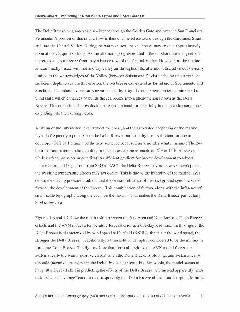
Figures 1.6 and 1.7 show the relationship between the Bay Area and Non-Bay area Delta Breeze
effects and the AVN model’s temperature forecast error at a one-day lead time. In this figure, the
Delta Breeze is characterized by wind speed at Fairfield (KSUU); the faster the wind speed, the
stronger the Delta Breeze. Traditionally, a threshold of 12 mph is considered to be the minimum
for a true Delta Breeze. The figures show that, for both regions, the AVN model forecast is
systematically too warm (positive errors) when the Delta Breeze is blowing, and systematically
too cold (negative errors) when the Delta Breeze is absent. In other words, the model seems to
have little forecast skill in predicting the effects of the Delta Breeze, and instead apparently tends
to forecast an “average” condition corresponding to a Delta Breeze almost, but not quite, forming.

Deliverable 3: Improving the Cal ISO Weather and Load Forecast
Scripps Institute of Oceanography (SIO) and Science Applications International Corporation (SAIC) 12
Figure 1.6. AVN Forecast Error and Delta Breeze. Compliments of Cal ISO.
D. Cal ISO Needs Assessment The project did not start with a focus on the Delta Breeze. An initial needs assessment was
completed involving a number of weather and load forecasters – short-term and long-term to
identify some of the key planning issues facing the Cal ISO. Meetings and interviews were used
to identify what the key short-term (0-7 days), intermediate term (7-14 days) and seasonal
forecast issues. The Cal ISO responded by providing a listing of short-term and long-term
weather and load forecasting planning issues. These are identified below.
Figure 1.7. Non-Bay Area AVN Forecast Error and Delta Breeze Effects
Bay Area Missed Forecasts vs Delta Breeze
y = -0.0078x2 + 0.7467x - 6.0497R2 = 0.736
-10
-5
0
5
10
15
0.0 5.0 10.0 15.0 20.0 25.0 30.0 35.0 40.0
Delta Breeze MPH
AV
N F
orec
ast E
rror
deg
F
Non Bay Area Missed Forecasts vs Delta Breeze
y = 0.0109x2 + 0.0701x - 4.5279R2 = 0.597
-10-8-6-4-202468
0.0 5.0 10.0 15.0 20.0 25.0 30.0 35.0
Delta Breeze MPH
AV
N F
orec
ast E
rror
deg
F
Deliverable 3: Improving the Cal ISO Weather and Load Forecast
Scripps Institute of Oceanography (SIO) and Science Applications International Corporation (SAIC) 13
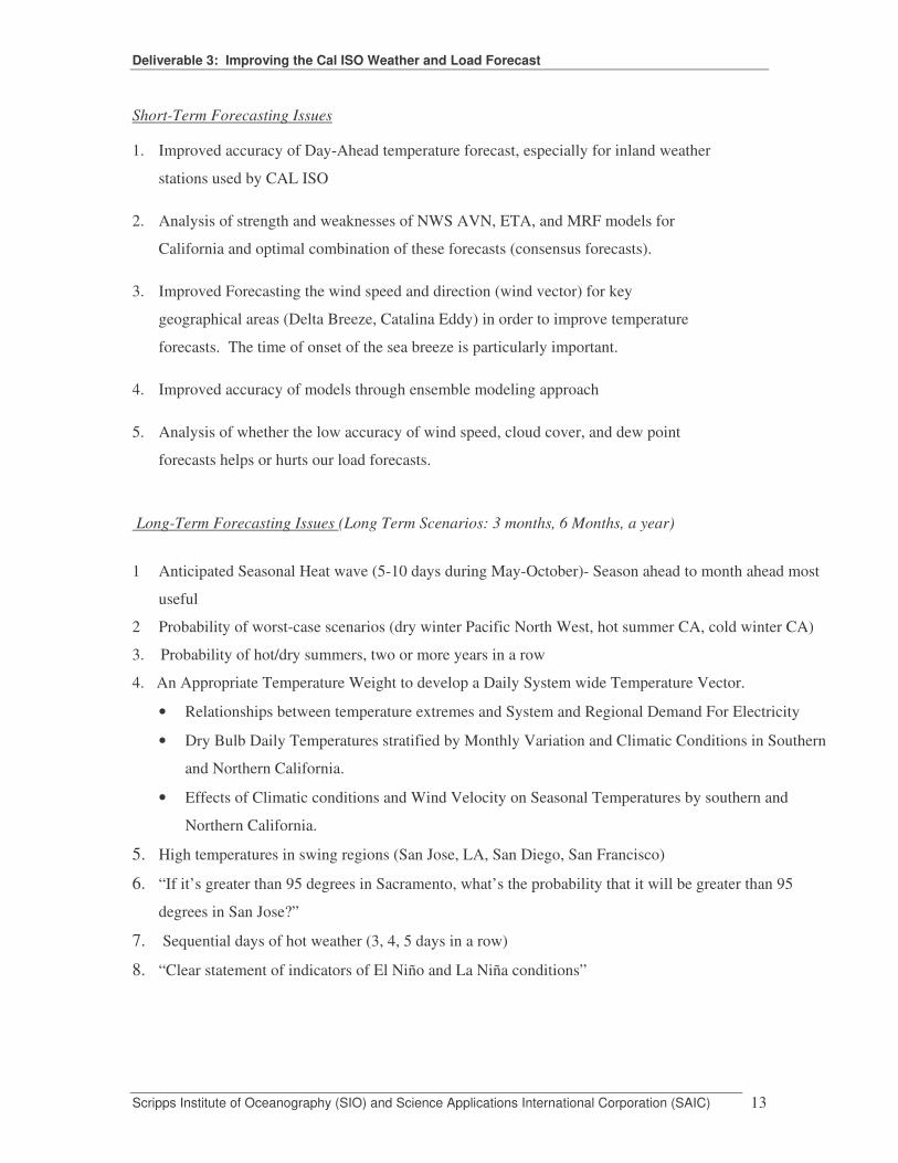
Short-Term Forecasting Issues
1. Improved accuracy of Day-Ahead temperature forecast, especially for inland weather
stations used by CAL ISO
2. Analysis of strength and weaknesses of NWS AVN, ETA, and MRF models for
California and optimal combination of these forecasts (consensus forecasts).
3. Improved Forecasting the wind speed and direction (wind vector) for key
geographical areas (Delta Breeze, Catalina Eddy) in order to improve temperature
forecasts. The time of onset of the sea breeze is particularly important.
4. Improved accuracy of models through ensemble modeling approach
5. Analysis of whether the low accuracy of wind speed, cloud cover, and dew point
forecasts helps or hurts our load forecasts.
Long-Term Forecasting Issues (Long Term Scenarios: 3 months, 6 Months, a year)
1 Anticipated Seasonal Heat wave (5-10 days during May-October)- Season ahead to month ahead most
useful
2 Probability of worst-case scenarios (dry winter Pacific North West, hot summer CA, cold winter CA)
3. Probability of hot/dry summers, two or more years in a row
4. An Appropriate Temperature Weight to develop a Daily System wide Temperature Vector.
• Relationships between temperature extremes and System and Regional Demand For Electricity
• Dry Bulb Daily Temperatures stratified by Monthly Variation and Climatic Conditions in Southern
and Northern California.
• Effects of Climatic conditions and Wind Velocity on Seasonal Temperatures by southern and
Northern California.
5. High temperatures in swing regions (San Jose, LA, San Diego, San Francisco)
6. “If it’s greater than 95 degrees in Sacramento, what’s the probability that it will be greater than 95
degrees in San Jose?”
7. Sequential days of hot weather (3, 4, 5 days in a row)
8. “Clear statement of indicators of El Niño and La Niña conditions”

Deliverable 3: Improving the Cal ISO Weather and Load Forecast
Scripps Institute of Oceanography (SIO) and Science Applications International Corporation (SAIC) 14
On May 28, 2003, CAL ISO “blew” their demand forecast by 7%. In addition, four of the major
California utilities also had severe errors in their forecasts anywhere from 5-7%. This resulted in
an unanticipated capacity load of 5000 Megawatts. This is the equivalent to the load required by
500,000 homes. This put a severe stress on the system, which nearly brought them to instability.
In order to meet the demand, they had to buy on the spot market, which can be up to $1000 a
Megawatt.
Forecast error was over 4%, whereas other commercial weather service providers were from 4%
to 7%. They speculated that the reason for the “blown” forecast could have been from valley and
inversion effects, not adequately modeled. This was a particularly critical time for them as the
summer peak was still far ahead of them, and they needed a sound plan for management of the
system.
Because the capacity of the supply is decreasing and there is so much “transmission-line
constraint” along the system which causes congestion and potential failure, they are now relying
on “demand-side management strategies” to balance the system. This strategy, which relies
heavily on accurate load forecasting (which relies on accurate weather forecasting), can buffer the
system by about 5-7%. The May 14th forecast error of 4-7% exceeded the amount of insurance
that the demand side management strategies buy them.
The May 14th incident was the catalyst for review of CAL ISO forecasting approaches. The
following analyses were performed:
1. CAL ISO reassessed which weather stations to use
a. Evaluated station representativeness
b. Used one year historicals and applied to four major areas
c. Increasing weather stations – considering more and interested in more ocean
stations.
d. Optimized new stations to use
e. Concerned about peak temp and load at top of hour of each day.
f. Applying this for each of the operational areas
g. Isolated bay area and non bay area loads
h. Bay area given a new weight
i. Use of civic center and Ontario versus LAX – latter is not representative.
j. Inland station data now driving S. California forecast

Deliverable 3: Improving the Cal ISO Weather and Load Forecast
Scripps Institute of Oceanography (SIO) and Science Applications International Corporation (SAIC) 15
k. Reassessing the variables to use-now use primarily temp, cloud cover and wind
speed
2. CAL ISO assessing improvements to model
a. RER neural net model to help with optimization
There is also a need to capture the timing and magnitude of the “Delta Breeze” in the load
forecast model. These winds carry the cool air from the ocean which cool the entire Bay area and
Central Valley up to 100 miles inland 10-20 degrees, and lower the electric load substantially.
Delta Breezes are prevalent from May 1 to September 30 during most years. It picks up in the
morning and is normal at night. It was estimated that during this time period, Delta breeze events
might happen nearly 50% of the time. According to the Cal ISO meteorologist, the Delta Breeze
is defined as winds greater than 12 mph at 190-280 degrees logged at Weather Station KSUU.
KSUU is not the only site to measure the Delta Breeze, but it probably gives the highest wind
speeds. Most of the Delta Breezes come in sequences from 3-5 days, which give an abrupt end to
the intense heat experienced in this area. The sequential nature of these events suggests that these
wind events are part of a larger atmospheric pattern that may be predictable on the larger scale. It
was expressed that a 24-hour lead-time for a prediction is necessary in order to be able to adjust
load. A sample of load data and one year of weather data was provided for KSUU. However,
KSUU does NOT have a good temperature correlation with load. Most weather forecast models
don’t pick up the onset or termination of these events. It was estimated that 83% of the transitions
were missed this past summer. Once these events start, they track them well. The NWS models
seem to pick up the change but not the magnitude of the change. Cal ISO gave a “rough estimate”
of weather error costs to be on the order of $100,000 per incident.
Other short-term findings:
1. Key time scales are two day ahead, hourly forecasts
2. Apply hourly forecasts to 30 minute interval estimates
3. Always doing forecasts for next three hours ahead—critical for final scheduling purposes
4. Tomorrow at 0800 AM commit for 8:00AM for day ahead. Also run at 10:00AM or 12 Z is
about 930A – update based on this.
5. Improving the 2-4 day forecast is the next most important. Can result in significant changes
in temperature in a 72-hour basis.
6. Back cast 2X’s weekly.
Deliverable 3: Improving the Cal ISO Weather and Load Forecast
Scripps Institute of Oceanography (SIO) and Science Applications International Corporation (SAIC) 16
7. A second major blown forecast for Sept 24th event. 11 degree F error. Cooler than projected.
Dropped 4,000 MW and as much as 10,000 MW.
8. Lack of historical data – only have 3 years of historical data.
9. Plan to back cast and retune forecast models.
The CAL ISO does long term forecasting for up to ten years. Annual/monthly forecasts for the
10-year period are used for their Frontier Function. They use regressions to select key predictor
variables. They run a simulation using 10 models, run the probability statistics and use for risk
management.
The long term forecast was viewed as accurate and useful. It is within 200MW of peak load.
They do not exceed 2% error. The key month for their forecast errors is September- very
uncertain time period. They also use the long-term forecasts from a resource planning for the
WECC and FERC. Key transmission planning issues include:
a. Use load densities by region for weighting
b. Use multi- economic variables
c. Use one in fifty probability (heat wave) estimates
They collaborate with CEC in long term forecasting. No joint forecast is developed however.
They publish a summer and winter two-year assessment. They use the RER model to forecast 24
hour ahead hourly forecast of loads. They use temperature, wind, degree-day, and dew point for
inland and central regions. Their model error average 2.3 in 2002 and 2.7 in 2003 (Summer),
although there are significant periods of a blown forecast. Error can be improved through
improved weather forecasts and the integrated load model – error source is about 50-50. The RER
model also creates a forecast for the next nine days and evaluates generation commitments for the
next nine days. CAL ISO evaluates large error through special statistical studies. They also
evaluate ways to improve peak load forecasts.
If the CAL ISO is going to truly be able to evaluate the benefits of a climate forecast in its
operations, then their models need to be optimized to incorporate new forecast information. An
ensemble model-testing project has begun that uses the days with large forecast errors as "bad
days" for ensemble model testing. The temperatures in the attachment are weighted average of
weather station temps as follows: SFO=.05, OAK=.05, CCR=.27, LVK=.27, SJC=.36.

Deliverable 3: Improving the Cal ISO Weather and Load Forecast
Scripps Institute of Oceanography (SIO) and Science Applications International Corporation (SAIC) 17
The CAL ISO reports the following problems in using the various national weather forecasting
models:
� AVN-MOS will under forecast maximum daily temperature when there has been and
increase in temperature over four degrees from the prior day – it is estimated that 83% of
the days are usually lower than expected.
� For those days, which experience a four percent reduction in maximum daily temperature
from one day to the next, the forecast is over predicted 76% of the time with an average
difference of 4.3 degrees.
� Other biases have been reported with the ETA-MOS and MRF-MOS.
The main conclusion is that MOS generally underestimates the magnitude of temperature
changes. Sometimes there may be as much as a 15 degree F error. A way to tackle the under-
forecasting and over-forecasting problems might be to develop a special set of MOS equations
from the AVN Model output, which are designed to minimize the under and over-forecasting,
while allowing the average error to increase a little. This would be much more valuable for
electric utilities. This has a direct economic benefit to electric utilities because (a) major under-
forecasting requires the utility to buy generation in the high-priced hourly market and could cause
blackouts if not enough energy can be purchased or transported. (b) major over-forecasting
incurs additional costs for purchasing excess ancillary services and for starting generator units
unnecessarily. CAL ISO estimated that in one year, over-forecasting cost $1M for ancillary
services alone. The costs for the generation starting are probably 10-15 times that amount.
Technical approaches which are being considered for this task are:
1. Use of ensemble forecasts to forecast major changes in temperature
2. Statistical analysis of NWS AVN MOS and ETA MOS forecasts to develop correction factors
for temperature rise and fall suited for electric utilities
3. Develop a model, which is optimized for better forecasting the significant temperature changes,
especially for inland stations during the summer.
E. Proposed Case Study - Improved Short Term Load Forecasting of the “Delta Breeze” Phenomenon The Cal ISO uses weather forecasts for two primary markets:
1. Hour Ahead Market – for the hour-ahead market, we use hourly weather forecast for
next 48 hours, updated hourly. The hour-ahead market closes 3 hours before the hour
Deliverable 3: Improving the Cal ISO Weather and Load Forecast
Scripps Institute of Oceanography (SIO) and Science Applications International Corporation (SAIC) 18
of operation, so the next three hours weather forecast is critical. This market operates
24/7.
2. Day Ahead Market – for the day-ahead market, we use hourly weather forecast for
the next 8 days, updated hourly. However, the next 48 hours are critical. The use of
weather forecasts for the day ahead market begins at 6AM PT and ends at 12 Noon
PT. This market operates 365 days per year.
3. Weather Variables – our RER forecast engine uses the following hourly forecast and
observed weather variables, updated hourly:
a. Temperature
b. Dew point
c. Cloud cover
d. Wind speed.
Deliverable 3: Improving the Cal ISO Weather and Load Forecast
Scripps Institute of Oceanography (SIO) and Science Applications International Corporation (SAIC) 19
2. Project Objectives, Literature Search and Approach
A. Objectives of Case Study The objectives of this research investigation are to:
1. Improve the predictability and load forecast associated with Delta Breeze events in the non-
Bay area (i.e., excluding the San Francisco Bay area) as treated in the CAL ISO 24- hour (or
day-ahead) load-forecasting model. This will involve attributing a proportion of hourly
forecast error in the CAL ISO model to the Delta Breeze.
2. Quantify the economic benefits of this improved treatment of Delta Breeze effects in terms of
estimating the avoided costs for unanticipated supply requirements—whether supply is over-
or under-forecasted.
The time interval for this analysis is hourly for the period March 20, 2001, through October 14,
2003 (this may be extended to November and December 2003, and into the first quarter of 2004).
B. Summary of Approach The approach taken to improve the forecasting of the Delta Breeze dynamic is summarized
below:
1. Complete literature search
2. Develop techniques or an index to measure Delta Breeze events. This includes acquiring and
checking data pertaining to weather station reporting archives
a. Develop and test Delta Breeze Index, includes exploratory research into the statistical
correlates of weather predictors and the advent of Delta Breeze
b. Test indices using Cal ISO model
c. Complete iterative analyses testing weather station error tests, the validity and predictive
value of an index of Delta Breeze effects and load forecasting model error improvements.
3. Determination of the economic value of improving predictions of Delta Breeze effects.
What follows is a description of each of these steps.
C. The Cal ISO Review of the Delta Breeze Phenomenon In summer, the northwest winds to the west of the Pacific coastline are drawn into the interior
through the Golden Gate and over the lower portions of the San Francisco Peninsula.
Immediately to the south of Mount Tamalpais, the northwesterly winds accelerate considerably

Deliverable 3: Improving the Cal ISO Weather and Load Forecast
Scripps Institute of Oceanography (SIO) and Science Applications International Corporation (SAIC) 20
and come more nearly from the west as they stream through the Golden Gate. This channeling of
the flow through the Golden Gate produces a jet that sweeps eastward but widens downstream
producing southwest winds at Berkeley and northwest winds at San Jose; a branch curves
eastward through the Carquinez Straits and into the Central Valley. (read: Delta Breeze). Wind
speeds may be locally strong in regions where air is channeled through a narrow opening such as
the Carquinez Strait (Fairfield is best measurement), the Golden Gate (SFO is best measurement),
or San Bruno Gap (SFO is best measurement). For example, the average wind speed at San
Francisco International Airport from 3 p.m. to 4 p.m. in July is about 17 knots, compared with
only about 7 knots at San Jose and less than 6 knots at the Farallon Islands.
The sea breeze between the coast and the Central Valley commences near the surface along the
coast in late morning or early afternoon; it may be first observed only through the Golden Gate
(so wind vector at SFO may be good predictor). Later in the day the layer deepens and intensifies
while spreading inland. As the breeze intensifies and deepens it flows over the lower hills farther
south along the Peninsula. This process frequently can be observed as a bank of stratus "rolling
over" the coastal hills on the west side of the Bay. The depth of the sea breeze depends in large
part upon the height and strength of the inversion. The generally low elevation of this stable layer
of air prevents marine air from flowing over the coastal hills. It is unusual for the summer sea
breeze to flow over terrain exceeding 2000 feet in elevation.
Carquinez Strait Region
The only major sea level pass through California's Coast Range is found in the Bay Area. Here
the Coast Range splits into western and eastern ranges. Between the two ranges lies the San
Francisco Bay. The gap in the western coast range is known as the Golden Gate, and the gap in
the eastern coast range is the Carquinez Strait. These gaps were originally cut by rivers that are
part of the drainage system from the Sierra Nevada mountains runoff. Besides allowing water to
flow to the ocean, these gaps allow air to pass into and out of the Central Valley.(via the Delta
Breeze)
The eastern gap, the Carquinez Strait, extends from Davis Pt in Rodeo to Martinez, ending at
Suisun Bay. The term "Carquinez Strait" is often loosely used to include the region east to
Antioch. At sea level, the strait is one to two kilometers wide, with terrain immediately north and
south reaching 500 to 600 feet.

Deliverable 3: Improving the Cal ISO Weather and Load Forecast
Scripps Institute of Oceanography (SIO) and Science Applications International Corporation (SAIC) 21
Prevailing winds are from the west in the Carquinez Straits, particularly during the summer.
During summer and fall months, high pressure offshore, coupled with thermal low pressure in the
Central Valley, (pressure difference between SFO and SAC measures this) caused by high inland
temperatures, sets up a pressure pattern that draws marine air eastward through the Carquinez
Straits almost everyday. The wind is strongest in the afternoon because that is when the pressure
gradient between the East Pacific high and the thermal low is greatest. Afternoon wind speeds of
15 to 20 mph are common throughout the straits region, accelerated by the venturi effect setup by
the surrounding hills. Annual average wind speeds are 8.2 mph in Martinez, and 9.5 to 10 mph
further east.
D. Literature Review of Delta Breeze (sic "sea breeze") The prediction of sea breezes has received extensive study around the world (Abbs and Physick,
1992; Simpson, 1994). Descriptions of this phenomenon have been recorded as early as 480 BC
in the writings of the Greek military historian, Plutarch, and independently in the work of
Aristotle and Theophrastus. However, understanding and modeling the mechanisms underlying
sea-breeze development has been most intensive since WWII with the advent of large scale
computing and routine detailed data collection. Much of this recent effort has been motivated by
concerns over forecasting localized storms, or the transport and dispersion of pollutants through
these sea breeze events in coastal areas. Most recently, the temperature drops associated with sea
breezes have been linked to patterns of energy usage.
All sea breezes initiate under the same conditions (Abbs and Physick, 1992; Simpson, 1994). Sea
breezes result from the contrasting thermal response between land and water surfaces. Diurnal
variations in temperature are much greater over land masses than over bodies of water. During the
day, heat from the land surface is distributed upwards by mixing resulting in a pressure
differential between land and sea. As the pressure aloft over land becomes higher, a compensating
high-level outflow of air from near-coastal land areas to those over water develops. This outflow
results in a surface pressure fall over a coastal strip of land and a corresponding increase in the
pressure over a coastal strip of sea. A pressure gradient is then set up between sea and land, and
results in a predictable low-level flow onshore. This circulation cell begins near the coast in the
morning and expands both landward and seaward throughout the day until cell collapse occurs
with nightfall. The thickness of the marine air component is usually approximately half of the

Deliverable 3: Improving the Cal ISO Weather and Load Forecast
Scripps Institute of Oceanography (SIO) and Science Applications International Corporation (SAIC) 22
vertical extent of the cell, but at any given location this depth varies with the time of day and
thickens as the day progresses. On average, the vertical extent of the sea-breeze (i.e., marine air
flowing on-shore) is greater in tropical zones than temperate, where depths average between 200
and 500 meters.
Additional observation has shown that this mechanism is not limited to marine coastal areas. Sea-
breeze type circulation cells can develop over any large body of water such as the Great Lakes
((Biggs and Graves, 1962; Lyons, 1972). Similarly, such circulation has been observed in
connection with large rivers (Zhong and Takle, 1992). Therefore, this simple mechanism may
exist in many more settings than previously observed, and have far greater impacts on local
weather conditions than previously recognized. Any setting defined by differential heating
resulting in development of a pressure gradient could host a circulation cell. For example, a
small-scale circulation cell resulting from localized heating over paved urban areas (“a heat
island”) could set up altering local weather conditions.
Observation and numerical modeling of the phenomenon have resulted in the understanding that
this very simple mechanism is subject to a number of different factors that affect development,
areal extent, and longevity. The interaction between topography and different mesoscale
phenomena, such as a sea-breeze, must be understood in order to predict the penetration of a sea-
breeze cell inland (Zhong and Takle, 1992; Heggem, et al., 1998). Orography (i.e., mountains) is
one of the major factors influencing the areal development and longevity of a “sea-breeze.”
Several researchers have confirmed that the existence of a slope (and/or a mountain) near shore
will affect a sea-breeze circulation cell (Walsh, 1974; Sumner, 1977; Kitada, et al., 1986).
Mountain/valley wind mechanisms can result in the acceleration of wind velocities associated
with sea-breezes as well as shift the time of maximum wind velocity. These winds combined with
a sea-breeze may form a strong, combined flow late in the day and early evening, and result in
greater penetration inland (Mahrer and Pielke, 1977; Abbs, 1986). Further, rates of advection
inland of sea air have been shown to be greatest up the larger river valleys from a coast (Sumner,
1977). This relationship has been observed in California through the Golden Gate, Petaluma Gap
and the Carquinez Strait (Fosberg and Schroeder, 1966). However, river valleys that are too deep
will tend to act as topographic barriers as a result of the development of anabatic winds off the
slopes.
In addition to mountainous coastal terrain, irregularity of coastlines has been shown to also affect

Deliverable 3: Improving the Cal ISO Weather and Load Forecast
Scripps Institute of Oceanography (SIO) and Science Applications International Corporation (SAIC) 23
the development of a sea-breeze. Convergence or divergence of land- and sea-breezes depends on
the curvature of the coast (Abbs and Physick, 1992). Sea-breezes diverge on concave seawards
coasts, while the reverse is true on convex coastlines. Along the California coast (a convex coast),
it has been demonstrated that both easterly and westerly winds are deflected upwards in the
convergence zone and result in strong updrafts. These updrafts increase the strength, areal extent,
and longeviity of the sea-breeze circulation cell. Where coast lines change direction suddenly,
such as a gulf or deep bay, two sea-breezes may develop. One is actually a bay breeze. In
combination the two may serve to either impede sea-breeze front advection, or conversely
promote. Coastal geometry in relationship to larger scale meteorological conditions determines
the effect.
The development of sea-breeze circulation cells is highly influenced by the various types of
prevailing synoptic conditions and thermal stratification (Estoque, 1962). Synoptic conditions are
defined by large-scale or regional winds and atmospheric stability. Synoptic winds will affect not
only the formation of a sea-breeze front but also its subsequent movement (Simpson, et al., 1977).
Since a vertical mixing component is essential to the establishment of sustained sea-breeze
circulation, a circulation cell can only develop in a relatively weak gradient wind field, and a
sufficiently strong synoptic wind can prevent development of a sea-breeze (Neumann and
Mahrer, 1971; Planchon and Cautenet, 1997).
The effects of four different synoptic regimes on sea-breeze development have been recognized
(Arritt, 1993). When onshore synoptic flow occurs (i.e., large-scale flow in the same direction as
the sea breeze), convergence frontogenesis is suppressed and the circulation cell will collapse.
Under calm to moderate opposing synoptic flow, a positive feedback is realized between the
convergence frontogenesis and the strength of the front. The convergence zone is located a region
of near-neutral stability so that large vertical and horizon velocities can develop. These conditions
result in the most intense sea breezes with the greatest inland penetration. Under strong opposing
synoptic flow, the convergence zone is typically located in a statically stable environment. As a
result vertical motion is suppressed, and the sea breeze develops, but no inland penetration
occurs. Finally, under very strong opposing synoptic flow, convergence is no longer capable of
intensifying the horizontal temperature (and pressure) gradient. The sea breeze remains entirely
offshore and will have relatively small vertical velocities, reducing the ability of the sea breeze to
trigger deep convection. In effect, no sea breeze can develop, and all flows are offshore.
Therefore, in order to recognize a sea breeze, the identification of the local to mesoscale onshore

Deliverable 3: Improving the Cal ISO Weather and Load Forecast
Scripps Institute of Oceanography (SIO) and Science Applications International Corporation (SAIC) 24
components as opposed to synoptic-scale gradient flow is required (Banfield, 1991). However,
other factors such as the local intensity of solar irradiance at the surface and the maximum land-
sea temperature contrast result in the seasonality of sea-breeze circulation cells.
Other factors have been identified as important in the development of sea-breeze cells. The
earth’s rotation (i.e., the Coriolis force) and friction have been shown to affect the intensity of
sea-breezes, but are unimportant in determining the geometry as are synoptic wind patterns
(Rotunno, 1983; Dalu and Pielke, 1989; Bechtold, et al., 1991; and, Xian and Pielke, 1991).
Inertia and friction both contribute to the reduction of inland penetration and sea-breeze intensity.
In low latitudes (less than 30 degrees), friction is a major controlling factor of the amplitude and
horizontal extension of sea-breeze flow. Vegetative cover will also affect sea-breeze penetration
(Planchon and Cautenet, 1997). For example, forested surfaces will result in greater turbulence,
which intensifies thermal exchange, and reduces the intensity of a sea-breeze. Further, in addition
to dictating seasonality, the degree of insolation (i.e., latitude dependence of solar gain) will
affect the frequency of occurrence (Gustavsson, et al., 1995). Both frequency and intensity of sea-
breezes will increase if the coastal terrain consists of a large flat surface with the greatest
potential for solar gain.
During the summer months, the climate in Central California is characterized by “monsoon”
conditions (Fosberg and Schroeder, 1966). This condition is locally known as the “Delta Breeze,”
and can set up for multiple-hour periods for several days running. This phenomenon initiates as a
“sea breeze” off of the Pacific. Streams of marine air from this source are funneled through the
Golden Gate into San Francisco Bay, and through the Petaluma Gap from Bodega to San Pablo
Bay. In San Pablo Bay, the two streams merge and move through the Carquinez Strait into the
Central Valley. Pressure and temperature gradients set up between high-pressure areas offshore
and the thermal trough in the interior. However, the “Delta Breeze” does not follow the classic
model of “sea breeze” development.
Detailed analysis indicates that topography and synoptic conditions play an extensive role in the
frequency and inland penetration of the “Delta Breeze.” Frenzel (1962) described a series of
diurnal changes in air temperature, wind speed, and pressure across the Valley. From examination
of these changes, and other data, Frenzel drew the conclusion that topography plays a crucial role
in defining the development of the “Delta Breeze.” Air in the valley appears to oscillate in phase
with that near the coast, and that in the valley differential heating at the coast line and the diabatic

Deliverable 3: Improving the Cal ISO Weather and Load Forecast
Scripps Institute of Oceanography (SIO) and Science Applications International Corporation (SAIC) 25
heating of the valley floor combine to produce a tertiary circulation. This tertiary circulation is
well developed in area extent and depth, and differs between the north and south ends of the
valley.
In addition to the pronounced affects of topography, synoptic patterns also have a controlling
effect on the “Delta Breeze” (Fosberg and Schroeder, 1966). Those patterns determine the
thickness of the marine air layer, and the strength of the monsoon winds. Days of pronounced
cooling in the Sacramento and San Joaquin valleys are linked to the development of an extremely
deep marine layer. This development coincides with the presence of a trough aloft. However,
when the Pacific high extends into the northwest, days are warmer at both of these localities. To
distinguish between afternoon cooling resulting from monsoon winds as opposed to the sea
breeze, the rate of advection (i.e., rate of invasion) of marine air was calculated and mapped
across the area. This analysis indicated that much of the cooling attributed to sea breezes was in
fact local in origin and probably associated with the tertiary circulation patterns. As a result of
both the topographic effects and the synoptic effects, the “Delta Breeze” is not easily predictable.
Within the Central Valley of California, because of all of these effects, sub-regions of localized
weather develop and weather patterns are harder to predict.
2. Techniques for Characterizing Sea Breeze Days
In order to characterize what constitutes a “sea-breeze” day, various methods have been applied.
The earliest studies were primarily observational and developed estimates of the frequency of
occurrence of a sea-breeze at a given location relative to other locations (e.g., Simpson, J.E., et
al., 1977). Still others have attempted to use the physical characteristics of a sea-breeze front as
regressors in a predictive linear relationship (e.g., Connor, 1997; Frysinger, et al., 2002). These
models have described the relationship between wind speed and predictors such as humidity,
cloud cover, and changes in dry bulb temperature. Most of these modeling attempts rely on
surface weather observations, and with one or two exceptions, ignore synoptic effects that can
mask a true “sea-breeze” day. Finally, other earlier attempts at characterizing sea-breeze days
have relied on the construction of an index (Biggs and Graves, 1962; Lyons, 1972). For example,
to characterize lake breezes around the Great Lakes, an index expressing a relationship between
the inertial and buoyancy forces was constructed. This index characterizes the dominant force,
and if the buoyancy force becomes large, the stage is set for establishment of a lake breeze. In
backcasts, this index approach has been over 90% accurate in prediction of sea-breeze days.

Deliverable 3: Improving the Cal ISO Weather and Load Forecast
Scripps Institute of Oceanography (SIO) and Science Applications International Corporation (SAIC) 26
Similarly, Fosberg and Schroeder (1966) created an advection index to evaluate the penetration of
marine air into Central California.
More recent work on the area of determining what constitutes a “sea-breeze day” have relied on
more sophisticated statistical and sampling methods. Doppler lidar has shown itself to be a useful
technique for the identification of sea breeze fronts in California (Banta, 1995). More
sophisticated statistical techniques have included development of time-series filters for various
factors (e.g., Borne, et al., 1988). The use of this type of approach allows for the inclusion of
synoptic variations, changes in wind direction, and changes in humidity either in front of or
behind a sea-breeze front. However, this type of method is site-specific and restrictive. Other
researchers have applied factoral analysis, including principal component analysis, canonical
correlation analysis and singular value decomposition, to finding coupled patterns in climate data
(Bretherton, et al, 1991). These approaches have allowed greater exploitation of available
observed data, but do have method-specific shortcomings. For the characterization of sea-breezes,
singular value decomposition has been successfully applied to radiometric data coupled with
surface data (Bigot and Planchon, 2003).
Additional discussions with other local weather forecast practioners in the Sacramento area
yielded the following list of variables that they use to produce a daily forecast at 10:00AM every
morning for the following day1:
• 500 mb height pattern (Ridge or trough--strength, timing, location)
Vorticity minimums and maximums (multiple stations throughout the area; strength,
timing, location)
• Pressure gradient between Reno and San Francisco
• Pressure gradient between San Francisco and Sacramento (same as the Fenzel article)
• Pressure graident between Redding and Las Vegas.
• 850 mb temperature (Oakland)
• 850 mb wind direction (Sacramento)
• Coastal marine layer depth
1 Conversations with Sonoma Tech, who has been forecasting the delta breeze for the Sacramento air quality program for about 5 years. (December 21, 2003).
Deliverable 3: Improving the Cal ISO Weather and Load Forecast
Scripps Institute of Oceanography (SIO) and Science Applications International Corporation (SAIC) 27
• Location of the thermal low (Very important! And this is sustained by Fosberg and
Schroeder).
The one overriding factor that appears to exist, which makes it difficult to predict the delta
breeze, is this key finding: very subtle changes in meteorology can have a profound influence on
the delta breeze strenght, timing, depth, and penetration.
The literature search showed that on the load forecasting side, the following steps are used to
forecast Delta Breeze:
• Test pressure gradients in Frenzel, 1962.
• Test diurnal dry bulb temperature between selected stations with several lags (24, 48,
etc.)
• Test advection variable found in Fosberg and Schroeder, 1966, for key stations.
• Test diurnal changes in different between dry bulb and dew point temperatures.
• Incorporate proportion of load into weighting scheme for temperature composite.
D. Conclusions The major conclusions from a review of the Cal ISO experience and based on the literature search
are as follows.
1. The Delta Breeze is strongly influenced by large-scale synoptic weather patterns that move
into California from the North Pacific ocean.
2. There is a substantial amount of uncertainty in predictions of the direction, speed and
sustainability of the Delta Breeze effect.
3. NOAA AVN model does a poor job of forecasting Delta Breeze events 24 hours in advance.
This may be due to the strong influence of small scale topography (unresolved by the model)
on the Delta Breeze – both the coastal hills and the Carquniez strait are important, and the
hills are only ~500 m high, while the strait is only 1-2 km wide.
4. The Delta Breeze has some similarities with other sea breezes, and there are useful insights
on how to attempt to capture this dynamic for California.
5. Delta Breeze is a complex interaction of synoptic Pacific, coastal, atmospheric pressure,
differential thermal forcing, and topographical dynamics. It is likely this interplay of factors
that make the Delta Breeze particularly difficult to predict.

Deliverable 3: Improving the Cal ISO Weather and Load Forecast
Scripps Institute of Oceanography (SIO) and Science Applications International Corporation (SAIC) 28
6. Extensive modeling and tracking of these events are occurring in the immediate Bay Area –
although the rigor and sophistication varies.
7. There is a tremendous need to address these issues either in the AVN or through some other
ensemble forecasting medium.
Deliverable 3: Improving the Cal ISO Weather and Load Forecast
Scripps Institute of Oceanography (SIO) and Science Applications International Corporation (SAIC) 29
3. Analysis of Delta Breeze Causes, Measurement and Forecasting Issues A. Background This section presents both a descriptive, heuristic approach to investigating the Delta Breeze
phenomenon as well as a more statistical approach to evaluating a method to improve the
forecasting of the Delta Breeze. Methods for improving load forecast accuracy for the Cal ISO
are also evaluated. First the more inductive and descriptive approach is presented. This is
followed by the statistical approach. Chapter 4 presents the economic value of the potentially
improved approach.
B. Scripps Institution of Oceanography Exploratory Investigation Into Delta Breeze Dynamics The Scripps Institute of Oceanography investigated the Delta Breeze phenomenon looking at
wide ranging synoptic factors. Data from buoys off the California coast were examined, along
with radiosonde observations at Oakland airport. In making a Delta Breeze forecast, the
investigation found that:
a) The buoy data off the California coast is not, by itself, sufficient to predict the onset
of the Delta Breeze.
b) Despite the lack of reliable day-ahead predictors obtained to date, there is still
potential to use the analysis information to create a useful predictor that can help
determine the magnitude of Delta Breeze effects. These data may provide useful clues on
the type of patterns to look for, particularly in large-scale antecedent synoptic patterns.
c) Delta Breeze patterns tend to run to completion statewide in a reasonably predictive
fashion once they have begun. If one were able to get days 2 and 3 of statewide patterns
correct, this would be very valuable. This investigation is continuing.
d) Another question is sub-day forecasting of the event. Even a 6 hour-ahead predictor
would still be valuable for the current day generation scheduling. This evaluation is
Deliverable 3: Improving the Cal ISO Weather and Load Forecast
Scripps Institute of Oceanography (SIO) and Science Applications International Corporation (SAIC) 30
continuing; it may be more amenable to the local, station-based analysis than is the day-
ahead forecast.
An additional key issue to be investigated in this project is the AVN MOS Corrector
issue. It appears that AVN MOS typically under estimates Delta Breeze events. There is
a need for the AVN MOS forecasts for 2001 and 2002 to further analyze and to make
sure that 2003 was not an anomaly. There is clearly a need to build a better corrector.
The project team is now pursuing the data and the extractor to accomplish this task. In
addition, NOAA/NWS was contacted in order to find out how the NWS builds the AVN
MOS equations. Are the equations area-wide and do they use a regression, which
minimizes the average more than the extremes? Since the load forecast objective is to
minimize the extremes, it makes perfect sense to have a custom set of MOS equations to
meet this objective. This is very valuable to the Cal ISO given the high costs associated
with all types of Delta Breeze events.
The following conclusions can be made based on an index of the Delta Breeze constructed from
wind speeds at Fairfield (KSUU station):
• Large scale simultaneous characterization of the delta breeze is robust, with a signal that
extends over the majority of the state.
• This large size implies the regional synoptic circulation will have a determining influence
on the event, unlike some other more local air-sea breezes.
• Local relationships at stations bear this out -- there are strong contemporaneous
correlations with the Delta Breeze, but the local antecedent relationships are very poor, as
the local situation does not reflect (in advance) the incoming synoptic patterns.
• The NCEP MRF (Medium Range Forecast) ensemble members seem to be poor in
predicting the delta breeze. The overall tendency is to over-predict a consistent onshore,
synoptic-scale flow that gives a model analogue of "delta breeze", but apparently captures

Deliverable 3: Improving the Cal ISO Weather and Load Forecast
Scripps Institute of Oceanography (SIO) and Science Applications International Corporation (SAIC) 31
little of the temperature differential vs. topographic barrier nature of the actual delta
breeze. In other words, it is forecasting ventilating onshore breezes for the wrong reasons.
• Incorrect behavior in this particular way is fairly consistent across the ensemble members.
• The AVN model errors from 2003 suggest that the worst (much warmer than predicted)
days have a mild tendency to come in periods preceeding actual Delta Breezes. Ending of
actual breeze events does not tend to cause the large negative (warmer than predicted)
errors.
• More historical AVN data would be needed to confirm this, but this suggests that the model
tends to produce the worst (warmer than predicted) errors when TODAY is NOT a delta
breeze day and the FORECAST is that tomorrow WILL be a delta breeze day. (i.e., over-
predicted onset of delta breeze conditions.)
C. Analysis, Approach and Results This analysis first involved an exploratory investigation into the Delta Breeze phenomenon taking
into account the earlier completed literature search. Scripps Institute of Oceanography
investigated Delta Breeze activity and in particular the key prior conditions that might exist a few
days ahead of a Delta Breeze event.
The approach involved the following steps:
1. Obtain data (station; radiosonde; global reanalysis)
2. Construct Delta Breeze index base on "standard definition" (-> load forecast)
3. Characterize Delta Breeze based on initial index
4. Iterate – is a superior index possible?
5. Characterize predictivity of optimal index.
The data sources included:
• Station data. ~150 western U.S. stations; hourly temperatures, winds, pressure. Not
corrected (quite raw). 1993-2004. These data are courtesy of the CEC archive collected
by SIO’s Larry Riddle.
Deliverable 3: Improving the Cal ISO Weather and Load Forecast
Scripps Institute of Oceanography (SIO) and Science Applications International Corporation (SAIC) 32
• Groisman: 134 California stations, daily Tmax, Tmin, precip; also hourly winds
corrected for anenometer height for the years ~1948 to 2002.
• Radiosonde: Oakland station. These data are taken twice daily (0 & 12Z), and the
archive extends from 1990 through today. This data give observed vertical structure of
atmosphere in a key location.
• Global: NCAR/NCEP Reanalysis 2. This consists of many fields every 6 hours, global,
3-D, 1979-2002.
The weather stations used are presented in Figure 3.1.
The Delta Breeze index used here is based on a standard definition that includes season, wind
speed, time of day, and wind direction at Fairfield, California (station KSUU). Specifically, an
hourly observation is taken to indicate a Delta Breeze condition if the following four conditions
are satisfied. 1) The wind speed at KSUU is > 12 mph. 2) The wind direction at KSUU is
between 190 and 280 degrees North. 3) The time of day is between 10 am and 4 pm local time,
inclusive. 5) The time of year is between May 1st and Sep 30th, inclusive. Further, a Delta Breeze
day is defined if at least 4 of the 7 possible hours (10 am to 4 pm) during the day experience
Delta Breeze conditions. In practice, it was found that the great majority of days have either most
(6 or 7) hours as Delta Breeze hours, or very few hours (1 or less). The cutoff criterion of 4 hours
was chosen mainly from considerations of missing data, which otherwise would have excluded
more days from the analysis. Using Groisman and Larry Riddle's CEC archive data, the index
extends from 1948 to end of 2003. The most interesting thing from index itself is prevalence of
"breeze spells", i.e., MUCH more likely to have runs of breeze days than you expect by chance.
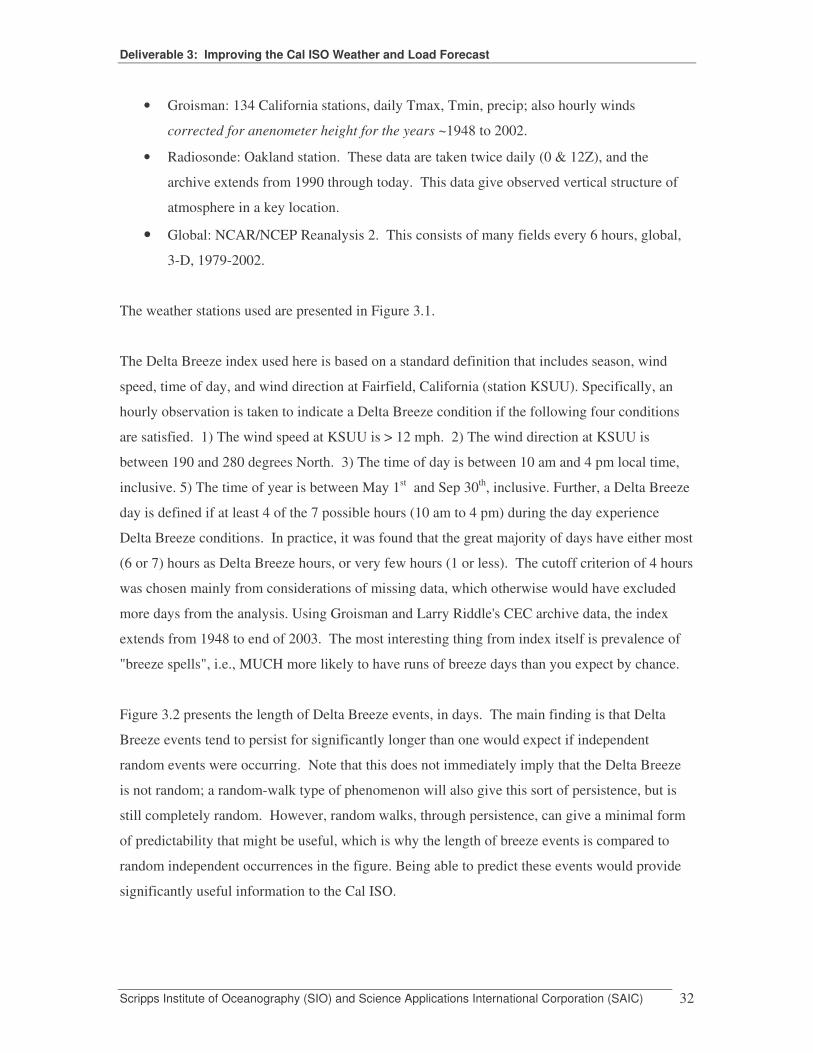
Figure 3.2 presents the length of Delta Breeze events, in days. The main finding is that Delta
Breeze events tend to persist for significantly longer than one would expect if independent
random events were occurring. Note that this does not immediately imply that the Delta Breeze
is not random; a random-walk type of phenomenon will also give this sort of persistence, but is
still completely random. However, random walks, through persistence, can give a minimal form
of predictability that might be useful, which is why the length of breeze events is compared to
random independent occurrences in the figure. Being able to predict these events would provide
significantly useful information to the Cal ISO.

Deliverable 3: Improving the Cal ISO Weather and Load Forecast
Scripps Institute of Oceanography (SIO) and Science Applications International Corporation (SAIC) 33
Figure 3.1. CEC Weather Stations Used.
Deliverable 3: Improving the Cal ISO Weather and Load Forecast
Scripps Institute of Oceanography (SIO) and Science Applications International Corporation (SAIC) 34
Figure 3.2. Distribution of the Length of Delta Breeze Events
Most of the following analysis is done in the form of composites rather than regressions --
composites are much better at handling episodic, non-linear events. In other words, the data was
separated into two classes – days during which (according to the Delta Breeze index described
above) a delta breeze occurred, and days where no Delta Breeze was found. A further analysis
was done to examine differences between days when the Delta Breeze is present but weak, as
opposed to days when the Delta Breeze is present and strong. This was done by retaining only
Delta Breeze days in the analysis, and then forming three classes by terciling on the wind speed at
KSUU. The resulting classes will be referred to as “weak”, “normal”, and “strong” Delta Breeze
days.
Figure 3.3 shows a particular example of winds where there is no Delta Breeze – in this case, for
September 25, 2002. On this day, winds carried hot air down the central valley, and power

Deliverable 3: Improving the Cal ISO Weather and Load Forecast
Scripps Institute of Oceanography (SIO) and Science Applications International Corporation (SAIC) 35
consumption (driven mainly by air-conditioner loads) was high (an average of 7962 MW hrs over
the day in the non-Bay area).
Sep 25, 2002: No delta breeze; winds carrying hot air down CaliforniaCentral valley. Power consumption high.
Figure 3.3. Non-Delta Breeze Condition
By comparison, Figure 3.4 shows the next day, when a Delta Breeze starts up. There is strong
on-shore flow, so that the winds carry cool marine air into the heart of the central valley.
Average power consumption on this day wass 7453 MW hrs in the non-Bay area, over 500 MW
hrs less than the previous day.
Sep 26, 2002: Delta breeze starts up; power consumption drops 500 MW compared to the day before.
Figure 3.4 Day With Delta Breeze Present

Deliverable 3: Improving the Cal ISO Weather and Load Forecast
Scripps Institute of Oceanography (SIO) and Science Applications International Corporation (SAIC) 36
The thickness of the marine layer has an important effect on the development of the Delta Breeze.
Because a number of different factors are involved in developing the breeze (synoptic scale
weather patterns, temperature differential between the ocean and interior, and the topographic
effects), the marine layer thickness does not by itself determine if a Delta Breeze will occur, but a
thick layer is nonetheless associated with Delta Breeze events. This is illustrated in Figure 3.5.
The left panel is vertical temperature (rightmost thick black line) and dew point (leftmost thick
black line) profile during on September 26 2002, the non-breeze day illustrated above. The right
hand panel shows the same thing for the next day, when the Delta Breeze was going strongly.
The thickness of the marine layer is generally taken as the distance from the surface to the
temperature maximum; on 26 Sep (left panel; non-breeze day) the top of the marine layer extends
to only 940 mb, while on 27 Sep (right panel; breeze day) the top of the marine layer is at 880
mb. A thicker marine layer has at least two effects; first, the greater mass of marine air is better
able to retain its characteristics in the face of mixing with the hot, dry central valley air as the air
advects inland. Second, the thicker layer makes it somewhat easier for the topographic barriers
around the bay area to be surmounted; although obviously this also depends on the large scale
flow field and overall vertical stratification.
Figure 3.5. Role of the Marine Boundary Layer Contributing to Delta Breeze.
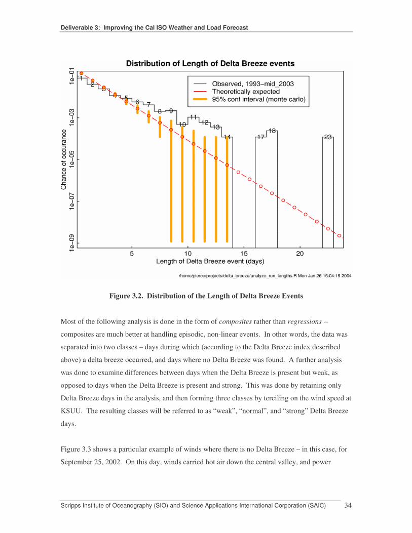
The statewide influence of the Delta Breeze is shown in Figure 3.6. This figure comes from the
two-class composite analysis; i.e., it shows composite temperature anomalies (degrees C)
experienced during Delta Breeze days (defined using the index described previously), relative to
Deliverable 3: Improving the Cal ISO Weather and Load Forecast
Scripps Institute of Oceanography (SIO) and Science Applications International Corporation (SAIC) 37
non-breeze days. It is not surprising that the cool temperatures push inland from the San
Francisco bay area towards Sacramento, as this is the classic behavior of a Delta Breeze. What
perhaps is more interesting is that the composite values are large state-wide, even as far south as
Bakersfield and as far north as Redding.
The implications of this large-scale pattern should be thought through carefully. Many
investigators have shown that a classic sea breeze is actually encouraged by off-shore flow (e.g.,
Aritt, 1993). However, one might expect that were purely local air-sea temperature contrasts the
sole force driving the Delta Breeze, that such a large-scale pattern would not be seen. On the
other hand, while on-shore flow tends to suppress a “true” sea breeze, such flow will still have a
tendency to advect cool marine air on shore, providing a ventilating effect, and might from a local
observer’s viewpoint appear to be a “true sea breeze”. The fact that the Delta Breeze has the
large-scale pattern shown in Figure 3.6. suggests that the synoptic scale weather patterns have a
strong influence on the Delta Breeze. This complicates prediction of the event, as local
relationships cannot then completely determine whether or not a breeze will develop; the
incoming weather patterns will be crucial as well.
Source: Scripps Institution of Oceanography.
Figure 3.6. -class composite: Breeze vs non-Breeze Days.
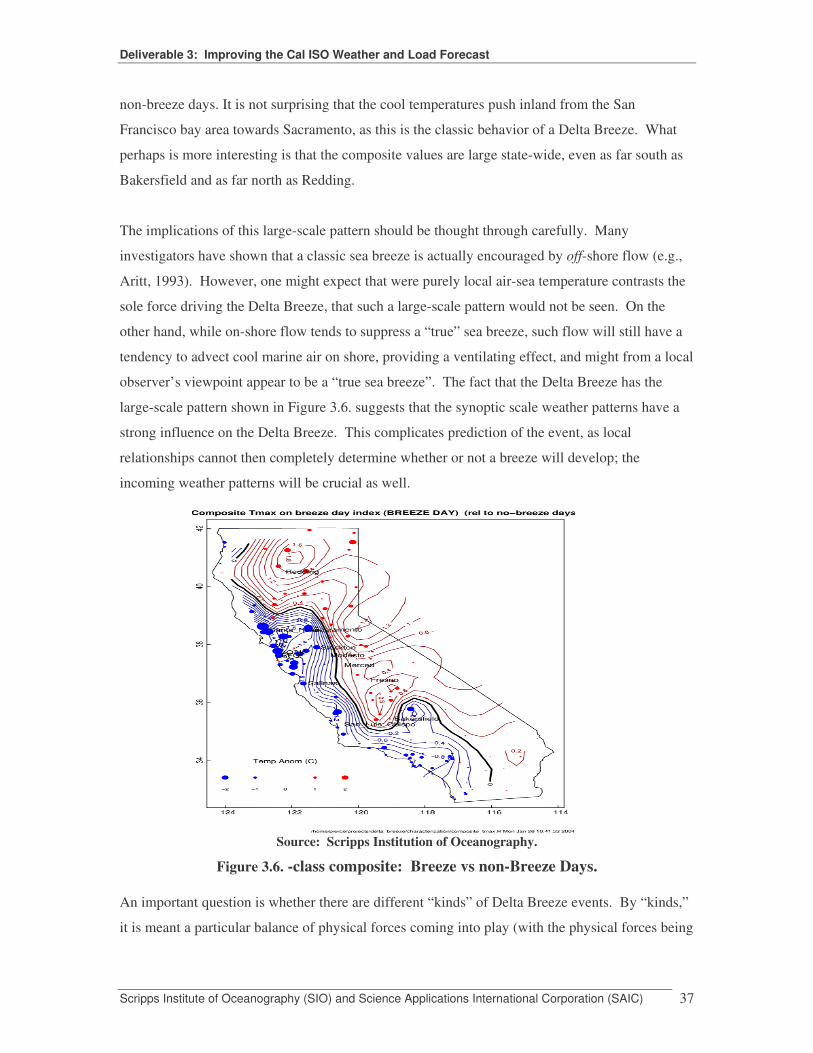
An important question is whether there are different “kinds” of Delta Breeze events. By “kinds,”
it is meant a particular balance of physical forces coming into play (with the physical forces being
Deliverable 3: Improving the Cal ISO Weather and Load Forecast
Scripps Institute of Oceanography (SIO) and Science Applications International Corporation (SAIC) 38
such things as the synoptic scale pressure and flow, the differential ocean-land temperature
contrast, topographic effects, and so on.) If there were different kinds of breezes, they would
have to be studied differently, rather than being treated as one specific phenomenon. One way
this can be tested is by seeing if different strengths of Delta Breeze appear to be different. For
example, one could imagine that weak events are characteristically different from strong events.
This is examined in Figure 3.7. Shown are the composite temperature anomaly fields (degrees C)
over California for Delta Breeze events in the weakest (left panel), middle (center panel), and
strongest (right panel) terciles, according to wind speed at Fairfield (KSUU). Only days marked
as being “Delta Breeze days” according to the criterion described above are included in the
analysis. The result shows that there is no systematic difference in expression of the Delta Breeze
based merely upon how strong the breeze is. This does not completely rule out the possibility
that there are different “kinds” of Delta Breeze – it is possible to imagine many causative factors
that somehow happen to co-vary simultaneously, producing the result shown in Figure 3.7 – but
such an explanation seems unlikely. The far more straightforward interpretation is that Delta
Breeze events are predominantly of one single kind, and can be expressed either more weakly or
strongly. Of course, this does not imply that Delta Breeze events are either simple or easy to
predict. Also, one could imagine other ways of testing for different “kinds” of breezes; for
example, multi-day events might be different from single day events, or breezes that start early in
the day might be different from ones that start late in the day. The strength criterion was chosen
because our primary purpose is to predict the strength of delta breezes (and hence their influence
on electricity load), rather than their onset time or duration.
The above two figures show the expression of the Delta Breeze over California. However, it is
also important to note that the vertical structure of the atmosphere during Delta Breeze events is
characteristically different than during days experiencing no Delta Breeze. This is illustrated in
Figures 3.8. Data for this Figure comes from the radiosonde observations at Oakland airport.
Observations are made at 0 and 12 Z, which is 4 AM and 4 PM local standard time. For these
figures, the 4 PM local time data have been used, as that better represents conditions during a
Delta Breeze day (which itself is taken over the period 10 AM to 4 PM).

Deliverable 3: Improving the Cal ISO Weather and Load Forecast
Scripps Institute of Oceanography (SIO) and Science Applications International Corporation (SAIC) 39
Lowest tercile Middle tercile Highest tercile
Figure 3.7. Relative Intensity of Delta Breeze Effects. Source: Scripps Institution of Oceanogrpahy.
Figure 3.8 (left panel) composites the vertical structure of relative humidity for strong (red curve),
medium (black), and weak (blue) Delta Breeze events. As above, Delta Breeze strength is
terciled upon wind speed at Fairfield (KSUU), with non-breeze days excluded. During the
strongest events, the figure shows that relative humidities are over 20 percentage points higher
than during non-breeze days. Even the weakest breeze events are 12 percentage points more
humid. The Figure also hints at the typical overturning structure that accompanies Delta Breeze
events; note that in the red curve (strongest events), the humidity is only enhanced at pressures
above 900 mb or so. At higher altitudes (pressures between 700 and 900 mb), humidities are
lower than usual. This is probably because the thermally-forced overturning circulation
associated with the Delta Breeze is returning dry air at altitude (flowing offshore and subsiding)
to replace the humid marine air that flows onshore along the surface. The temperature anomalies
(right panel) are in accord with this interpretation; as expected, near the surface the onshore flow
of cool marine air produces cooler than normal temperatures (by over 4 C for strong events),
while at mid levels, the temperatures are actually warmer than normal by up to 1.5 C.

Deliverable 3: Improving the Cal ISO Weather and Load Forecast
Scripps Institute of Oceanography (SIO) and Science Applications International Corporation (SAIC) 40
Source: Scripps Institution of Oceanography.
Figure 3.8. Left: vertical structure of relative humidity (%) anomalies for weak (blue), medium (black), and strong (red) delta breeze events. Right: same, for temperature anomaly (deg-C). Both measured at Oakland, CA. Figure 3.9 shows the relationship of historical marine layer depth and the incidence of Delta
Breeze. The table indicates that there is a distinct shift in the distribution of marine layer depth ,
which is thicker during Delta Breeze days as compared to non Delta Breeze days. This is not a
surprise; one of the factors contributing to a strong Delta Breeze event is the presence of a marine
layer thick enough to resist attrition by mixing with hot, dry central valley air as the leading edge
of the plume penetrates inland. Also, since the hills surrounding the San Francisco bay are
relatively low (400-500 m), a very thick layer would presumably have a better chance of flowing
right over this barrier. One of the motivations for examining this distribution was to evaluate the
ability of the marine layer depth to predict Delta Breeze events on a 1-day timescale.
Unfortunately, it did not turn out to have appreciable skill as a predictor.

Deliverable 3: Improving the Cal ISO Weather and Load Forecast
Scripps Institute of Oceanography (SIO) and Science Applications International Corporation (SAIC) 41
T Source: Scripps Institution of Oceanography. Figure 3.9. Marine Layer Depth and Presence of Delta Breeze Days.
The previous results, and others not shown here for brevity, suggest that local station data do not
give a good forecast of the upcoming Delta Breeze at a one-day lead time. This is not unexpected
given the discussion above about the importance of the synoptic scale flow to setting up
conditions that favor interior ventilation of the California central valley. It is, therefore, useful to
examine the synoptic scale precursors to Delta Breeze days; this is illustrated in Figures 3.10 and
3.11 for 500 mb geopotential height anomalies and surface pressure anomalies, respectively.
Focusing on the surface pressure anomalies first (Figure 3.10), it can be seen that breeze days are
associated with low pressure over Oregon and southeast Washington, combined with weak
elevated pressure over southern California. The sense of this pressure pattern is to encourage
onshore flow over the Bay Area. Again, it is important to note that traditional sea breezes are
encouraged by mild offshore flow; this is consistent with the picture drawn above that the Delta
Breeze is somewhat more complicated than a traditional, local sea breeze, and is strongly shaped
by synoptic scale onshore flow as well as by the thermal overturning of a traditional sea breeze.

Deliverable 3: Improving the Cal ISO Weather and Load Forecast
Scripps Institute of Oceanography (SIO) and Science Applications International Corporation (SAIC) 42
The 500 mb height anomalies (Figure 3.11) show a systematic progression of a trough into place
just off the coast of California as a Delta Breeze develops. Preliminary attempts to find this
pattern in forecast data, and use it for a forecast of the Delta Breeze, have had poor skill due to a
low signal to noise ratio.
Figure 3.10. Surface Analmolies for Larger Area Delta Breeze Events.
Figure 3.11. Larger Scale View of Anomolies Affecting Larger Area Delta Breeze Events.
Again with an eye towards seeing how Delta Breeze events evolve in time, Figure 3.12 shows the
evolution of California state-wide temperature patterns one day before the breeze event (left
panel), concurrent with the event (middle panel), and one day after the breeze event (right panel).
Probably the most interesting thing in these figures is again the suggestion that the Delta Breeze
is part of a synoptic-scale pattern that effects all of California. Presumably if the breeze were
only a local traditional sea breeze mediated by the gap in the mountains around the Carquinez

Deliverable 3: Improving the Cal ISO Weather and Load Forecast
Scripps Institute of Oceanography (SIO) and Science Applications International Corporation (SAIC) 43
straits, the time evolution would be confined to the Bay Area, and not extend fairly uniformly
throughout the state.
Figure 3.12. Larger Scale View of Anomolies Affecting Larger Area Delta Breeze Events.
All the previous results are examining the Delta Breeze on short timescales (a few days at most).
Yet longer timescale variability might be of interest to Cal ISO, either now or in the future. Some
questions of interest include: do all summers have an about equal number of breeze days? If not,
what is the characteristic spread between years? Can years with many breeze days be
anticipated? These questions will now be explored.
Figure 3.13 shows the number of Delta Breeze days by year, from 1940 to 2003 (middle panel).
Interestingly, there is a slow modulation of the number of breeze days, so that some years and
decades have distinctly more than others. Low pass filtered versions of the Delta Breeze
frequency (“DB.freq”) and intensity (“DB.int”) are shown in the upper part of Figure 3.14. As
can be seen, for example, the period around 1980 had a smaller number of events, and a weaker
average strength, than the period around 1990. The bottom panel of Figure 3.14 shows the
correlation of the frequency of Delta Breeze days with sea surface temperature (SST) anomalies
(i.e., departures from conditions typically observed at that time of the year) in the preceeding
January. The pattern that results, with warm temperatures extending across the central North
Pacific and a rim of cold temperatures along the west coast of the U.S., is characteristic of the
North Pacific Oscillation (“NPO”), also called the Pacific Decadal Oscillation (PDO).
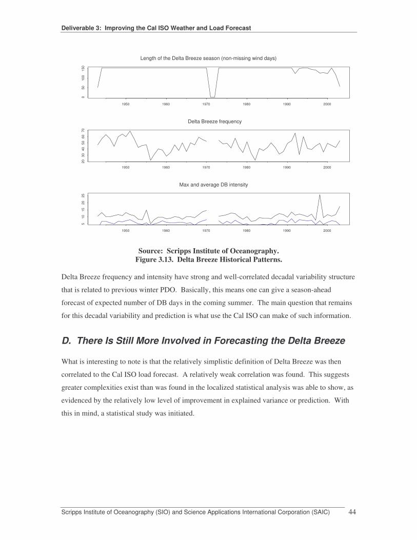
Deliverable 3: Improving the Cal ISO Weather and Load Forecast
Scripps Institute of Oceanography (SIO) and Science Applications International Corporation (SAIC) 44
Source: Scripps Institute of Oceanography. Figure 3.13. Delta Breeze Historical Patterns.
Delta Breeze frequency and intensity have strong and well-correlated decadal variability structure
that is related to previous winter PDO. Basically, this means one can give a season-ahead
forecast of expected number of DB days in the coming summer. The main question that remains
for this decadal variability and prediction is what use the Cal ISO can make of such information.
D. There Is Still More Involved in Forecasting the Delta Breeze What is interesting to note is that the relatively simplistic definition of Delta Breeze was then
correlated to the Cal ISO load forecast. A relatively weak correlation was found. This suggests
greater complexities exist than was found in the localized statistical analysis was able to show, as
evidenced by the relatively low level of improvement in explained variance or prediction. With
this in mind, a statistical study was initiated.
1950 1960 1970 1980 1990 2000
050
100
150
Length of the Delta Breeze season (non-missing wind days)
1950 1960 1970 1980 1990 2000
2030
4050
6070
Delta Breeze frequency
1950 1960 1970 1980 1990 2000
510
1520
25
Max and average DB intensity

Deliverable 3: Improving the Cal ISO Weather and Load Forecast
Scripps Institute of Oceanography (SIO) and Science Applications International Corporation (SAIC) 45
Figure 3.14. Decadal Delta Breeze Correlation With SST
The statistical design paralleled the existing CAL ISO load forecasting model, but also
incorporated the following alterations or additions:
� Addition of 10 weather stations: KRBL, KMAE, KSAC, KVCB, KSUU, KCCR,
KFAT, KVIS, KSBP, KSMX to the six original stations (KRDD, KMCE, KSTS,
KMYV, KPRB, KBFL) for a total of 16 in model. � Depiction of 3 load centers: Redding, Merced, Bakersfield instead of assuming one
load center at Merced.
� Creation 3 temperature composites using inverse of (distance from load center)2
� Use dry-adiabatic lapse rate of 3.3o F per 1000’ of elevation to adjust all temperature
measures to sea-level.
� Disaggregation of 6-hour average CDD and HDD into hourly measures.
1950 1960 1970 1980 1990 2000
2030
4050
6070
DB.freq low frequency evolution
150 200 250
020
4060
-1.0
0.0
1.0
Cor(freq, JanSST)
1950 1960 1970 1980 1990 2000
24
68
DB.int low frequency evolution

Deliverable 3: Improving the Cal ISO Weather and Load Forecast
Scripps Institute of Oceanography (SIO) and Science Applications International Corporation (SAIC) 46
Still More Analysis is Needed
While the analysis that was completed did not find any significant statistical improvement in
predicting the Delta Breeze, the results were somewhat positive, since they ruled out a number of
factors, and confirmed the econometric model (see below).
• An econometric load model parallel to ITRON, currently implemented at CAL ISO, has
been built for the CAL ISO non-Bay region for the period of March 20, 2000 to June 30,
2003.
– The model employs a simultaneous equation specification depicting total energy
for each day and an hourly equation. The model is solved using an iterative three-
stage least squares method.2
– All of the variables in the base case econometric model are the same as the CAL
ISO ITRON model. Definitions for those variables along with load-relevant data
was provided by CAL ISO (Dennis Gaushell).
– Weather data for 24 stations was provided from the Scripp’s Institution of
Oceanography. Those data originated from the METAR data sets routinely
collected by the National Weather Service. It should be noted that initial runs of
the econometric model were performed using the raw data, i.e., no imputation of
missing values. The implications of imputation and the choice of use of a data set
from a commercial vendor (Weather Bank) will be discussed in a later bullet.
• For a comparative test of the two frameworks using the same set of variables for a base
case, the econometric model exhibited on average a 2.2% lower (-2.2%) Mean Squared
Error.3 Both models were run without the “shift” variables that had been previously used
in the ITRON model to control for periods of substantially larger residuals. Instead of the
2 Judge, George G., et al., 1988. Introduction to the Theory and Practice of Econometrics, Second Edition. New York: John Wiley & Sons. Greene, William H., 1993. Econometric Analysis, Third Edition. Upper Saddle River, New Jersey: Prentice Hall. 3 The ITRON results were provided by Dennis Gaushell in an e-mail on February 28, 2004. The econometric results for a base case were provided by Lorna Greening on February 23, 2004.

Deliverable 3: Improving the Cal ISO Weather and Load Forecast
Scripps Institute of Oceanography (SIO) and Science Applications International Corporation (SAIC) 47
“shift” variables, the econometric model uses maximum and minimum daily temperature
(dry bulb and dew point) squared variables, and this probably results in the slightly better
results. Comparative runs with ITRON on Friday, February 27, 2004 indicated that
substituting this variable for the shift variable in ITRON had no significant impact on the
ITRON base case.
• Using an expanded set of weather stations (a total of 14) beyond the six currently used in
CAL ISO ITRON, results from the econometric model indicate that addition of additional
weather stations to the ITRON model could lead to an average potential reduction of as
much as 15.5% (-15.5%) in MSE. For this case, a weighting of the inverse of squared
distance from Merced, California was used.
In addition to the decrease in forecasting error, the addition of weather stations to the
current suite of stations has the following advantages:
– Review of the literature, and analysis by Scripps, indicates that the weather
patterns in the non-Bay area are heavily dependent upon localized factors and
conditions. As demonstrated by Scripps, weather patterns such as the “Delta
Breeze” cannot be dependably predicted using methods depending on meso-scale
features. The Scripps analysis has demonstrated a lack of persistence of
phenomenon that would be considered consistently predictable of a weather
pattern.
– The addition of new weather stations allows the further disaggregation and
identification of these localized patterns.
– Analysis indicates that the pattern of missing days or observations varies across
weather stations in the area. Increase in the number of stations should allow for
an increase in the number of useable observations. The temperature composite
can be re-weighted for missing observations more reliably.
• To further test for the potential impacts of local weather conditions, based on graphic
material provided by Scripps, and correlation analysis performed early on, three “load
centers” or temperature composites (3 for dry bulb and 3 for dew point temperature) were

Deliverable 3: Improving the Cal ISO Weather and Load Forecast
Scripps Institute of Oceanography (SIO) and Science Applications International Corporation (SAIC) 48
developed from the expanded set of weather stations. Those centers are Redding (Load
Center 1), Merced (Load Center 2), and Bakersfield (Load Center 3). Temperatures for
each center were adjusted using an adiabatic correction of 3o per thousand feet. This type
of normalization allows the combination of different weather stations into a single
“station” value.
Temperature composites were defined for each center based on an inverse of the distance
squared of a given station from a center; station membership in a center is independent,
i.e., no station appears in two centers. These temperature composites were then weighted
into a single composite based the proportion of load assumed for each center. The
defining of a single temperature composite for dry bulb and dew point was required by
the number of observations (i.e., degrees of freedom issue) available for analysis in the
raw METAR data. Using an imputed set of data may allow the disaggregation of
individual temperature aggregates by load center.
In addition to defining a temperature composite defined around load centers with
different weightings based on distance from the center and proportion of the load,
individual center variables for maximum daily dry bulb temperature squared (3 variables,
one for each center), maximum daily dew point temperature squared, and weighted cloud
cover (CAL ISO definition) were implemented in the energy equation. In the hourly
equations, weighted cooling (CDD) and heating (HDD) degree day variables were
defined by load center (3 variables for CDD; 3 variables for HDD) for each hourly
equation. Similarly build-up variables for previous days HDD and CDD (HDDBU and
CDDBU).
– This specification resulted in a decrease of 19.2% (-19.2%) average MSE over
the reference case. Or, an additional 3.8% reduction accrued over the case where
additional weather stations were added. Also, of note, the CDD, HDD, CDDBU,
HDDBU, maximum temperature squared variables, and cloud cover variables
defined by load center (3 each for each category) were of varying degrees of
significance, but different. That is, depending upon the equation, these variables
were highly significant. This indicates a difference between load centers.

Deliverable 3: Improving the Cal ISO Weather and Load Forecast
Scripps Institute of Oceanography (SIO) and Science Applications International Corporation (SAIC) 49
– It should again be noted that these results were originally obtained from the raw
METAR data and confirmed with a set containing imputed data, and no re-
weighting of the temperature composites for missing observations. Reweighting
of the temperature composites for missing stations (a possibility with the
expanded set of stations) further confirmed these results, and indicated that more
improvements through reductions in forecast error were possible.
The methods of imputation used for the final estimation data set included
averaging between hours for one missing observation in a series, or interpolation
based on the rate of change between adjoining data for longer series of missing
observations. A criterion for “bad days” of at least ten imputed observations in
sequence was used in determining the necessity for re-weighting (i.e., excluding
a station for a specific day and reweighting the others) of the temperature
composites for a given day. This is a more restrictive criterion than currently
used by CAL ISO; but, with the addition of weather stations, no loss of degrees
of freedom occurred, and actually was gained.
With the limited time remaining, CAL ISO experimented with defining two load centers using the
existing six weather station series (KRDD, KMCE, KSTS, KMYV, KPRB, KBFL).
Using the observed temperature data for the existing six weather stations, the Cal ISO developed
weighted average temperatures for North (KRDD, KSTS, KMYV) and South areas (KMCE,
KPRB, KBFL), using the distance-based weights that were provided. A total of 20 days had to be
marked off (common to all stations) due to bad data. These missing days were the result of
telemetry problems between the ISO and the Weather Bank; use of the original METAR station
series does not have this problem, because very rarely are sufficient stations out of service
simultaneously. Then two cases were run: a) the Itron model optimizes the weighting of North
and South and b) using the fixed North-South proportion that was provided.
The Cal ISO then ran the tests without the shifts and obtained the following results for Standard
Error (average of 48 half-hour intervals):
• Current Model (Coastal and Inland weighted average temperatures): 235
• Model with distance-based weights for North and South (model decides weighting of
North and South): 234

Deliverable 3: Improving the Cal ISO Weather and Load Forecast
Scripps Institute of Oceanography (SIO) and Science Applications International Corporation (SAIC) 50
• Model with distance-based weights for North and South (fixed weights of .35 for North
and .65 for South): 240.
Then the tests were rerun with the shifts, which gave the following results (Average MSE for the
model):
• Current Model (Coastal and Inland weighted average temperatures): 176
• Model with distance-based weights for North and South (model decides weighting of
North and South): 179
• Model with distance-based weights for North and South (fixed weights of .35 for North
and .65 for South): 183.
The CAL ISO test of the concept of different load centers could not be termed conclusive. The
CAL ISO test of the two load center concept did not include the disaggregation of the cooling and
heating degree variables (nor heat build-up) and cloud cover variables into load centers. Both of
these classes of variables were significant in the econometric model. Nor did the CAL ISO tests
include the maximum and minimum temperature (dry bulb and dew point) variables. Where these
variables had been included in the econometric framework, they were significant and were
associated with MSE reductions for the overall model. Where these variables were disaggregated
into load centers in the econometric framework, even greater reductions in MSE occurred, and
varying degrees of significance indicated differences between the load centers.
There were some notable limitations with this analysis.
(1) No tests were requested in the later stages of the analysis for the differences in mean
variables between North and South. The Cal ISO selected North/South on the basis of the
availability of data from the existing weather stations.
(2) Also, the Ca ISO probably did not look at how the stations differed in lost days. The addition
of weather stations not only increases information in the model, but also allows for the potential
reweighting of stations to reduce the number of missing days.
(3) Although the results from the econometric model, particularly in the case where all weather-
related variables were disaggregated into load centers, indicated the potential effects of finer scale
weather features (e.g., pressure gradients) on predicting load, these effects were not tested.

Deliverable 3: Improving the Cal ISO Weather and Load Forecast
Scripps Institute of Oceanography (SIO) and Science Applications International Corporation (SAIC) 51
E. Conclusions The Delta Breeze is a very complex phenomenon that does have some elements of its mystery
known. However, the probabilities of Delta Breeze dynamics are highly variable and still
difficult to predict.
The research completed in this project has found that the Delta Breeze is caused by:
• Longer time scale/seasonal, and cyclical patterns
• More intermediate Pacific Ocean dynamics influence Delta Breeze influences that begin
to take shape in the Pacific Northwest and influencing events also in Southern California
• These events coupled with the highly uncertain humidity levels and pressure gradient
interacting with coastal and inland topography influence the direction and speed in which
the Delta Breeze goes inland.
• There are also another set of dynamics that occur pertaining to individual weather
stations along the path of the Breeze and how this influences the Breeze’s behavior in the
Central Valley can be another dynamic altogether.
• The AVN-MOS model is ill equipped to adequately forecast Delta Breeze events in its
current state. Significant interest should be devoted to understanding the current
algorithms and how they can be improved to capture the more complex events that are
known to occur.
What the Cal ISO wants out of this analysis is how this complex dynamic can lead to a better
Maximum Daily Temperature value, which is a key predictor in the Cal ISO load-forecasting
model. Currently, statistical approaches have shown little in the way of improved predictability
by themselves. It appears that the greatest potential improvement in forecasting Delta Breeze
effects is additional research on the larger synoptic dynamics, longer-term climate cycles, and the
use of an improved pressure index. Once improvements are made in these areas, there may be an
improvement in the use of statistical models.

Deliverable 3: Improving the Cal ISO Weather and Load Forecast
Scripps Institute of Oceanography (SIO) and Science Applications International Corporation (SAIC) 52
4. Estimation of the Economic Value of the Improved Forecasting of the Delta Breeze For the Cal ISO
A. Background As noted earlier, weather and load forecasting plays a valuable role in the planning and operation
of the Cal ISO. Both short-term and long-term forecasts are used. Long-term forecasts are used
for more transmission capacity and network upgrade planning. Short-term forecasting is used
more for estimating peak loads, scheduling generation and transmission flow and routings.
This case study has shown that the Delta Breeze phenomenon is a very uncertain event –
influenced by both longer term climatic dynamics, plus more immediate Pacific ocean-based
events that occur days in advance, only later to be further affected by topographic, pressure and
essentially unpredictable occurrences in the Central Valley.
The relationship, though, of Delta Breeze factors on maximum temperature levels – a key factor
used in Cal ISO load forecasting, is more known and highly depended on in making load
forecasts. When this project started, the economic costs associated with Delta Breeze-induced
maximum temperature errors were known to be significant, but how significant on an event
driven basis was less well understood. Through the cooperation and support of the Cal ISO,
largely working with Mr. Dennis Gaushell and other management, a better understanding of the
economic costs of temperature error and the cost of the error become more known.
The investigation into the economic costs of Delta Breeze effects is also illuminating from the
standpoint of how difficult it is to determine what the true costs are of weather forecast error.
Figure 4.1 illustrates these cost components. At the most fundamental level, the plant or power
plants that are dispatched on the margin that may or may not be necessary are the cost of forecast
error if such plants are not needed but were put on line and operating due to a higher load
forecast. However, the incremental generation used could have already been on-line or just
“spinning” for reliability purposes and not necessarily in use to meet loads. In this case, the cost
of the plant is not the start-up costs, which might average anywhere from $100,000 to $200,000,
if the unit had to be started and made ready for dispatch. When plants are already running, the
cost of the unit might be an average of $100,000-$800,000/event.

Deliverable 3: Improving the Cal ISO Weather and Load Forecast
Scripps Institute of Oceanography (SIO) and Science Applications International Corporation (SAIC) 53
The analysis shown below is that when using a limited data set – say for the summer 2003 time
period, and tracking less than 20 events, there are a host of factors that can cause the scheduling
and dispatching of power plants that have a wide range of causes and cost implications that go
well beyond weather forecast error. Thus, as one tries to isolate on a case-by-case basis the cause
of plant dispatch and the resulting costs, many factors contribute to this beyond the weather
forecast accuracy question. This means that the cost function and the resulting benefits from
improving weather forecasts might have independent drivers and costs (and hence benefits) that
may not directly benefit from improving weather forecast error. In the detailed sense – on a case
by case basis – this cost-benefit relationship is highly situational.
Now when a larger range of data points are amassed and central tendencies can be shown, there
may very well be some relationships and averaged values that can be used. This is what the
Figure 4.1 is attempting to show.
There is also the degree of load forecasting model error, which in the case of the Cal ISO is about
55% of total error, with weather the other portion. Tracking the mico-level events and costs can
be quite valuable to the Cal ISO in order to see if larger statistical profiles and ranges of the costs
and sources of error can be identified.
Alternatively, there is a more macro level of consideration that is possible. This would involve
using a more generalized proxy indicator that would use a sort of mean value of weather forecast
Plant/Network
SchedulerDecisions
Load ModelCorrections
Load ForecastModel
A. Plant ColdStart (Y/N)
B. Plant Spinning(Y/N)
Sum of Error Cost > t1+t2+tn
A. Conditions = Startup cost + operating costB. Conditions = Operating Costs
Weather ForecastError
Weather StationData Error
Weather ForecastModel Error
Figure 4.1 Macro and Micro-Level Approaches to Estimating the Cost of Weather Forecast Error
Plant/Network
SchedulerDecisions
Load ModelCorrections
Load ForecastModel
A. Plant ColdStart (Y/N)
B. Plant Spinning(Y/N)
Sum of Error Cost > t1+t2+tn
A. Conditions = Startup cost + operating costB. Conditions = Operating Costs
Weather ForecastError
Weather StationData Error
Weather ForecastModel Error
Weather ForecastError
Weather StationData Error
Weather ForecastModel Error
Figure 4.1 Macro and Micro-Level Approaches to Estimating the Cost of Weather Forecast Error
Deliverable 3: Improving the Cal ISO Weather and Load Forecast
Scripps Institute of Oceanography (SIO) and Science Applications International Corporation (SAIC) 54
error cost taking into account load forecast error and loadings on the Cal ISO power system. An
investigation into this aspect of valuing load forecast error was completed by the Cal ISO.
What follows is a review of these macro or averaged approach versus the more micro or
situational approach.
B. Approach The Cal ISO talked to the schedulers and operators of generation plants and identified specific
case study situations where an over or under forecast occurred. In addition, they supplied a
frequency distribution of occasions where weather forecasts were either over- or under-projected.
An average cost of forecast error was estimated. The basis of the cost of forecast error were built
up by the type of generating plant or purchase power on the margin that would set the marginal
cost of all plants being dispatched at that time. The costs calculated for this analysis for under and
overforecasting were the directly measurable costs; there were other indirect costs, such as impact
on marginal costs, which were very difficult to calculate and were not included. However, it is
believed that these costs would not significantly affect the overall result. The cost of weather
forecast error is that proportion of error attributed to weather data and model error net of load
forecast error. Again, this averages about a 45-55 split. Documentation of these plant costs were
shared with SAIC, but remained in the hands of the Cal ISO. From this regression curves and
estimates were calculated. (See Figures 4.2 and 4.3 below).
C. Economic Value of Improved Estimation of Delta Breeze and Its Effect on CA ISO Load4
For the sample period of Delta Breeze resulting in either an over or under forecast, regression
equations were developed. Figure 4.2 shows the regression equation for underforecasting actual
loads. The chart shows a relatively small number of incidences in terms of the peak day forecast
estimates. Most of the forecast error is between 1000-2000 MW. There was one extreme event
that was about 5000 MW.
<Confidential figure removed> Figure 4.2. Summer 2003 Cost of Under-forecasting Load

Deliverable 3: Improving the Cal ISO Weather and Load Forecast
Scripps Institute of Oceanography (SIO) and Science Applications International Corporation (SAIC) 55
Discussions with Dennis Gaushell of Cal ISO shed some additional light on how this curve
should be interpreted. There are a large number of underforecast errors less than 2000 MW that
show little or no associated cost. This is because there are typically generator units already
running that can cover this level of underforecast load. However, days where the underforecast is
extreme, such as on May 28th, 2003 (with an underforecast of ~5300 MW), incur significant
costs. There are also noticeable effects associated with operators adjusting the load forecast,
based on their strong tendency to avoid underforecasting. This tendency occurs because in
addition to economic factors, the operators must maintain overall system reliability, and a
shortage of generation is a serious problem. For example, without operator adjustment, there
would be an equal number of over- and under-forecast days. Instead, we see more overforecast
days. This has the effect of reducing the number of underforecast days (days when the forecast
load was lower than actually transpired) and increasing the overforecast days (when forecast load
was higher than actually experienced).
Figure 4.3 shows the regression equation for the cost of over-forecasting load. The chart shows
that the Summer 2003 over-forecast cost is much more dispersed. Average forecast error is
around 2000-3000 MW. One outlier at 5505 has been omitted from this analysis. This point
indicates a much lower cost for the overforecast than it “should have” experienced. This is
consistent with operator intervention; if the operator thought the forecast was too high, he/she
might adjust it down. Including this single point drops the R2 of the best linear fit from 0.31 to
0.02; moreover, it significantly changes the calculated intercept of the best-fit line in the event
that the line is not forced to go through the origin. (Note that in both Figures 4.1 and 4.2, the
best-fit curves have been forced to go through the origin.) This is at odds with what we expect,
which is that zero overforecast should incur zero cost. When the point is omitted, there is little
difference in the best-fit trend whether or not the curve is forced to go through the origin. Based
on this, it was decided that the point likely shows operator intervention, and that excluding it
would give a more accurate estimate of the costs associated with overforecasting. The residual
variance unexplained by the trend line is likely influenced by the fact that the marginal cost of
electricity supplies is highly volatile, depending on the current market conditions. For instance,
when temperatures are high over the entire western U.S., the incremental cost of obtaining an
additional MW is much higher than if temperatures are generally cool over the western U.S., even
if both situations have the same underforecast load error.
4 This section is based on the contribution of Dennis Gaushell of the California ISO.

Deliverable 3: Improving the Cal ISO Weather and Load Forecast
Scripps Institute of Oceanography (SIO) and Science Applications International Corporation (SAIC) 56
<Confidential figure removed> Figure 4.3. Summer 2003 Cost of
Overforecasting
Comparing Figures 4.2 and 4.3, one can see that costs for the extreme underforecast event can be
higher (on a basis of dollar per MW forecast error) than for an overforecast. Exactly how much
higher is hard to estimate, as there is really only a single instance in this data set of an extreme
underforecast day – May 28th, 2003. The uncertainty in this estimate must be considered very
large, as the particular set of events surrounding extreme underforecast days can be quite variable
and dependent on the regional situation, as described above. Still, the example of May 28th
clearly shows that the costs of underforecasting large events can be many times that of
overforecasting events with the same error.
To tie these cost curves to temperature forecast error, one needs a relationship between
temperature and daily peak load over the service region. This can be obtained from Figure 1.2
(source: “California ISO operations report, Board of Governors, June 6, 2003,” available at
http://www.caiso.com/docs/09003a6080/22/c9/09003a608022c993.pdf). This indicates that
between 80F and 100F, load in the Cal ISO service area goes up by ~530 MW/deg-F. The typical
temperature change associated with the Delta Breeze varies by location, time, and strength of the
breeze, as can be seen in Figures 3.6, 3.13, and 3.7, respectively. An average Delta Breeze
(middle strength tercile) gives temperature changes of the order 1.5 deg-C (2.7 deg-F) over much
of the inhabited coastal areas of California. This gives an estimate of an average Delta Breeze’s
effect on loads as ~1400 MW. An overforecast error of this size (i.e., if a breeze develops when
none was predicted) incurs costs of about $210,000. An underforecast error of this size (i.e., if
no breeze develops when one was predicted) can be seen from Figure 4.2 to give little error, due
to the combination of extra generating resources typically being available all the time, and
probably also the effect of operator “adjustment” towards overforecast conditions. A strong
Delta Breeze (highest strength tercile) is associated with temperature changes on the order of 2
deg-C (3.6 deg-F); this corresponds to an effect on load of ~1900 MW, with an over-forecasting
cost of about $290,000.
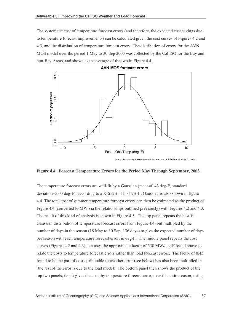
Deliverable 3: Improving the Cal ISO Weather and Load Forecast
Scripps Institute of Oceanography (SIO) and Science Applications International Corporation (SAIC) 57
The systematic cost of temperature forecast errors (and therefore, the expected cost savings due
to temperature forecast improvements) can be calculated given the cost curves of Figures 4.2 and
4.3, and the distribution of temperature forecast errors. The distribution of errors for the AVN
MOS model over the period 1 May to 30 Sep 2003 was collected by the Cal ISO for the Bay and
non-Bay Areas, and shown as the average of the two in Figure 4.4.
Figure 4.4. Forecast Temperature Errors for the Period May Through September, 2003
The temperature forecast errors are well-fit by a Gaussian (mean=0.43 deg-F, standard
deviation=3.05 deg-F), according to a K-S test. This best-fit Gaussian is also shown in figure
4.4. The total cost of summer temperature forecast errors can then be estimated as the product of
Figure 4.4 (converted to MW via the relationships outlined previously) with Figures 4.2 and 4.3.
The result of this kind of analysis is shown in Figure 4.5. The top panel repeats the best-fit
Gaussian distribution of temperature forecast errors from Figure 4.4, but multipled by the
number of days in the season (18 May to 30 Sep; 136 days) to give the expected number of days
per season with each temperature forecast error, in deg-F. The middle panel repeats the cost
curves (Figures 4.2 and 4.3), but uses the approximate factor of 530 MW/deg-F found above to
relate the costs to temperature forecast errors rather than load forecast errors. The factor of 0.45
found to be the part of cost attributable to weather error (see below) has also been multiplied in
(the rest of the error is due to the load model). The bottom panel then shows the product of the
top two panels, i.e., it gives the cost, by temperature forecast error, over the entire season, using
Deliverable 3: Improving the Cal ISO Weather and Load Forecast
Scripps Institute of Oceanography (SIO) and Science Applications International Corporation (SAIC) 58
the expected number of days with the given temperature forecast error. The total cost over the
season for all days is also noted in the bottom panel; in this case, it is ~$9.9M.
<Confidential figure removed> Figure 4.5. Costs Associated With Forecast Errors.
It should be understood that this is only a very rough estimate, since it makes many assumptions.
First, it assumes that temperature forecast errors in the Bay Area are representative of those in
the entire Cal ISO service region. This is probably too conservative; temperature swings in the
Bay Area are likely less than the average over the service region due to the moderating influence
of the ocean on Bay Area temperatures. It then seems probable that forecast errors in the region
will similarly show a smaller range of variability than those over the entire service area. Second,
only part of the variance in over- and under-forecast costs can be explained by the cost curves of
Figures 4.2 and 4.3. As noted above, operator adjustments are important, and the incremental
cost of power varies day to day. Third, the conversion of temperature forecast error to load
forecast error is only approximate, and is done here with a single, crude relation between
temperature and load.
Nevertheless, keeping these caveats in mind, Figure 4.5 still illustrates some general points of
interest. Most immediately noticeable is that the total cost of overforecast temperatures (the area
under the right-hand hump in the bottom panel of 4.5 is larger than the total cost of underforecast
temperatures. This is true even considering the influence of such extreme underforecast days,
such as May 28th, 2003. Basically, the small incidence of extreme events dominates over the
large cost of these events, making them less costly overall in the season than the much more
frequent moderate-sized errors. In fact, days when the forecast temperature is between 2.5 and
3.5 deg-F above actual account for the most costly days, taken over the entire season. This is
because they are seen rather often (the expected value is about 14 days/season), and their cost is
not insignificant (~$100,000 per day).
Another advantage of the analysis of Figure 4.5 is that it allows one to estimate what effect
changes in forecast skill have on total costs over the season. For example, a different mean and
standard deviation of temperature forecast model errors (top panel of Figure 4.5) will generate a
different total cost over the season. This can be calculated for an entire range of values, with the
result shown in Figure 4.6. The x axis in this figure represents the mean temperature forecast

Deliverable 3: Improving the Cal ISO Weather and Load Forecast
Scripps Institute of Oceanography (SIO) and Science Applications International Corporation (SAIC) 59
error (deg-F), while the y axis represents the standard deviation of the temperature forecast error.
The contours are the total cost, in millions of dollars, of temperature forecast errors over the
season. The current estimated values of temperature forecast error are shown by the large black
dot at (0.43, 3.05).
One potential use of this kind of figure is to evaluate in what manner the temperature forecast
should be adjusted for lower costs, and what the cost difference would be if that were done. The
optimal choice for improvement is perpendicular to the contour lines; in this case, moving
towards the point (0.4, 2.7). In other words, the best improvement would be found if any
decrease in temperature forecast standard deviation sd were accompanied by decrease in
temperature forecast mean m such that m = (2/3)sd.
Note: The black dot shows the estimated values for the current forecast. Figure 4.6. Cost (millions of dollars) As A Function of Temperature Forecast Error and Standard Deviation (deg-F).
Deliverable 3: Improving the Cal ISO Weather and Load Forecast
Scripps Institute of Oceanography (SIO) and Science Applications International Corporation (SAIC) 60
Another use of this figure is to estimate the cost savings obtained by an improved temperature
forecast. For example, moving from the current forecast to one with a mean error of 0.4 deg-F
and a standard deviation of 2.7 deg-F would decrease costs due to weather forecast error by
about $2M/year. This provides one estimate of the economic value of an improved temperature
forecast to Cal ISO.
The results show that when an over forecast generally occurs, the costs are much lower because
they have a higher proportion of potentially lower cost plants operating and potentially ones that
are already “spinning” which means the incremental costs are lower for using these plants and
dispatching them into the system. On the other hand, when there is an underforecast, the base
resource situation for the Cal ISO in terms of base generation availability is much more diverse.
There actually might be a much higher cost in starting up, dispatching and running plants to meet
this condition.
The data appear to indicate that other than these general patterns the actual cost per event are
highly variable. An alternative approach that examines episodes individually, rather than as an
averaged whole, would be the following:
• More closely investigate 13 of the actual under/over forecast days (from July to Sept)
used in the cost analysis to determine the proportion of model errors and weather errors.
• The analysis consisted of:
a. determining the hourly MW errors due to load forecast model and hourly MW errors
due to weather forecast, for each of the 13 days.
b. taking the absolute value of each hourly MW point
c. summing the absolute values for weather and for model (while this overstates the
total error because some hourly model and weather errors cancel, I believe the ratio
should not be affected)
d. calculating the ratio of total absolute weather error to total absolute weather error +
total absolute model error
The result was 0.45, i.e., weather error is 45% of the total error for these days. (The weather error
would have to be interpreted as applying to the days with major costs; in general the Cal ISO
believes that the weather error is a lower percentage of total error.)

Deliverable 3: Improving the Cal ISO Weather and Load Forecast
Scripps Institute of Oceanography (SIO) and Science Applications International Corporation (SAIC) 61
Next the distribution of load forecast errors was analyzed for the summer period and found that
there was no bias due to model or weather. Thus, the operators had shifted approximately 15
days out of under forecast category and 15 days into the overforecast category. Since the cost of
underforecasting appears to remain fairly low except for extreme events, the operators probably
increased the overall costs by shifting 15 days into the overforecast category, where costs are
reasonably certain.
For the analysis shown in Figure 4.2, the total cost of underforecasting in summer 2003 was
approximately $2,800,000. For overforecasting in Figure 4.3, the total cost of underforecasting in
summer 2003 was approximately $14,000,000, including an additional 25 overforecast events not
analyzed in detail.The Cal ISO also reports that the costs for excess purchases of ancillary
services (reserves and regulation) due to overforecasting, (which were calculated a year ago) were
about $848,000 for calendar 2002.
As a calibration data point, the Cal ISO reports that Duke Power was quoted as saying that
erroneous load forecasts cost a minimum of $8,000,000 per year. Duke is approximately half the
size of Cal ISO. So the total cost of load forecast error for Cal ISO of $17,648,000 is consistent
with the Duke number.
If one were to assume that the operator effect on the total under/over forecasts was neutral, this
leads to the conclusion that the cost of weather error is approximately equal to
0.45*($2,800,000for underforecast+$14,848,000 for overforecast ) or about $7,941,600. While
this applies to the summer period only, this is where the majority of Cal ISO costs occur due to
load forecast errors occur. Since summer 2003 was a typical year, the number of approx
$8,000,000 could be used may be used as an annual figure for the value of weather forecast.
D. The Role of Ensemble Forecasts: The Look Forward The Cal ISO reported that:
“the cause of the Sept 24 overforecast of 5505 MW was mostly weather forecast error. The costs were low because (a) the previous day was approximately the same load as forecast for Sept 24, so no new units were started for Sept 24, and hence, no startup costs and (b) the operators must
Deliverable 3: Improving the Cal ISO Weather and Load Forecast
Scripps Institute of Oceanography (SIO) and Science Applications International Corporation (SAIC) 62
have seen the major trend in load developing, and dropped units off before incurring substantial minimum load costs.”5
The Cal ISO also reported in internal correspondence that from reviewing the past few days in
mid September of 2003 that there was a classic southerly surge event in which long shore surface
pressure gradients reversed from northerly to southerly, and a deep marine layer was advected
onshore from south to north. This event was a low-level event, occurring almost entirely below
the 900-mb level.
The 850-mb temperatures above the marine layer were just as warm as they were during the
warming cycle last weekend. Tuesday was the first day of the cooling cycle - the models were
going for a cooling trend over the next couple of days. In making Wednesday's forecast on
Tuesday, a CA ISO senior forecaster followed the model ensemble (protocols established during
late AUG and early SEP) or average, which did show the cooling trend. The ensembles have
performed just as well, if not better than any individual model(s) over the prior couple of weeks.
For the 11 AM PT forecast update the senior forecasters compared the 00Z ensemble models
against the 12Z ensembles... and found that for the Bay Area and San Diego, the 12Z numbers
were 3 or 4 degrees cooler than the 00Z numbers, and knowing that a cooling cycle was
underway, opted to lower the forecasts to reflect the cooler 12Z numbers. The 12Z AVN on that
day showed much cooler temps for the Bay Area Wednesday than the other models, and since the
AVN has a well-known cool bias, and, has seldom out-performed the ensembles, it was rejected.
As it turns out , the 12Z Tuesday AVN was more accurate for Wednesday than the ensembles, but
this performance was a rare fluke, and it will usually not outperform the ensembles into the
future. The models always have problems handling low-level marine surges like this event. The
CA ISO believes that ensembles will be, over the long term, the safest way to go. This is the next
phase of the research for the CA ISO, along with a greater investigation into the larger synoptic
and coastal causal factors of Delta Breeze.
5 September 25, 2003 e-mail to Dennis Gaushell.

Deliverable 3: Improving the Cal ISO Weather and Load Forecast
Scripps Institute of Oceanography (SIO) and Science Applications International Corporation (SAIC) 63
5. Conclusions A. Overview This section presents the general findings of this case study. Implications for future research are
also provided. The key findings and implications address the entire value chain of weather
monitoring stations, data quality and edit checks, modeling and analytics.
B. Conclusions
1. A key forecast parameter for CA ISO load forecasting is temperature, which the Delta
Breeze can significantly affect. When the breeze runs strong it can lower forecasts
more than expected. When it suddenly changes or is non-existent, it can increase load
forecast, due to the rising temperatures.
2. Delta breeze and temperature variations are subject to many causal influences including
larger climatological, synoptic, seasonal/cyclical, the representativeness of weather
stations, time lapse, topography and other factors.
3. AVN does not do well predicting Delta Breeze
4. Using new weightings such as Root Mean Error do not add significant improvements in
reducing forecasting errors.

Deliverable 3: Improving the Cal ISO Weather and Load Forecast
Scripps Institute of Oceanography (SIO) and Science Applications International Corporation (SAIC) 64
5. Current neural net models do not pick up the slight changes in temperature and other
weather data in shoring a significant improvement in load forecasts.
6. Additional investigation is needed in constructing a better index of Delta Breeze
effects.
7. Data quality is a major issue as is the manner in which third party commercial weather
firms edit the data and document what is being done to replace missing data. A similar
problem exists in working with NOAA data sets, based on this project’s experience.
8. It is equally complex estimating the costs/benefits of weather/load forecast error, due to
Delta Breeze
a. A large cost variation is whether or not operators anticipate load events and
schedule plants ahead of the weather event, and then already have enough
spinning capacity available to meet the “lower probability” loads based on
model predictions
9. Major costs are associated with underestimating loads, most of which is weather
induced. Overforecasting loads are relatively less costly overall because lower cost
units are operating, relative to underforecasting loads.
10. Both sizeable underforecasting and the more frequent, but smaller, load forecast errors
are significant costs over time – much more than the lower incident underforecast
events
a. Most forecast error represents about 1000-2000MW. A very few extreme
errors of 5000MW and higher occur.
11. The average cost of over forecast is about $150/MW. However, for one extreme case
of an over forecast, the cost rose to $390/MW. Plant availability can cause these costs
to swing a lot.
12. The total cost of Delta Breeze induced load forecast error, due to the .45 weather factor
is associated with a seasonal cost of about $9.9 Million.
13. Improving the temperature forecast mean error by reducing it to about .4 deg-F vs. the
.45 deg-F and using a standard deviation of about 2.7 degree-F would save the Cal ISO
about $2 million/season.
C. Implications for Future Research Implications for future analysis includes the following:
1. Too few holidays in the short data series.

Deliverable 3: Improving the Cal ISO Weather and Load Forecast
Scripps Institute of Oceanography (SIO) and Science Applications International Corporation (SAIC) 65
• Suggestion: Combine all holidays into one variable.
• Result: Increase in significance to over 75% of all equations.
2. Fraction of daylight variable insignificant in over 50% of hourly equations.
• Suggestion: Restructure fraction of daylight time to more closely capture
behaviors depicted.
• Result: Increase in significance in majority of equations.
3. Separation and representation of two cycles.
• Seasonal cycle.
– Suggestion: Add total daily load by month (lagged one day) to
energy equation, e.g., January_ld, etc. Use no intercept.
– Result: Decrease in MSE.
• Weekly cycle.
– Suggestion: Add total load by weekday type (lagged one week), e.g.,
Monday_ld, Tuesday_ld, etc. Use no intercept so that all days can be
represented.
– Result: Decrease in MSE and increase in significance.
4. Drop shift variables since they are not based on observable information.
Deliverable 3: Improving the Cal ISO Weather and Load Forecast
Scripps Institute of Oceanography (SIO) and Science Applications International Corporation (SAIC) 66
Appendix A
Selected References. Abbs, D. J. "Sea-Breeze Interactions Along a Concave Coastline in Southern Australia:
Observations and Numerical Modeling Study." Monthly Weather Review 114(May), 1986 831-48.
Abbs, D. J. and W. L. Physick. "Sea-breeze Observations and Modelling: A review." Australian
Metrological Magazine 41, 1992 7-19. Arritt, R. W. "Effects of the Large-Scale Flow on Characteristic Features of the Sea Breeze."
Journal of Applied Meteorology 32(1), 1993 116-25. Banfield, C. E. "The Frequency and Surface Characteristics of Sea Breezes at St. John's,
Newfoundland." Climatological Bulletin 25(1), 1991 3-20. Banta, R. M. "Sea Breezes Shallow and Deep on the California Coast." Monthly Weather Review
123(December), 1995 3614-22. Bechtold, P., et al. "A Numerical Investigation of the Influence of Large-Scale Winds on Sea-
Breeze- and Inland-Breeze-type Circulation." Journal of Applied Meteorology 30, 1991 1268-79.
Biggs, W. G. and M. E. Graves. "A Lake Breeze Index." Journal of Applied Meteorology
1(September), 1962 474-80. Bigot, S. and O. Planchon. "Identification and Characterization of Sea Breeze Days in Northern
France Using Singular Value Decomposition." International Journal of Climatology 23, 2003 1397-405.
Borne, K., et al. "A Method for Finding Sea Breeze Days Under Stable Synoptic Conditions and
Its Application to the Swedish West Coast." International Journal of Climatology 18, 1998 901-14.
Bretherton, C. S., et al. “An Intercomparison of Methods for Finding Coupled Patterns in Climate
Data.” Journal of Climate 5, 1992 541-560. Connor, G. J. "Statistical Short-term Forecasting Technique for Wind and Temperature in a
Coastal Tropical Location (Townsville)." Australian Metrological Magazine 46, 1997 257-65.
Dalu, G. A. and R. A. Pielke. "An Analytical Study of the Sea Breeze." Journal of the
Atmospheric Sciences 46(12), 1989 1815-25. Estoque, M. A. "The Sea Breeze as a Function of the Prevailing Synoptic Situation." Journal of
the Atmospheric Sciences 19(May), 1962 244-50. Fosberg, M. A. and M. J. Schroeder. "Marine Air Penetration in Central California." Journal of

Deliverable 3: Improving the Cal ISO Weather and Load Forecast
Scripps Institute of Oceanography (SIO) and Science Applications International Corporation (SAIC) 67
Applied Meteorology 5, 1966 573-89. Frenzel, C. W. "Diurnal Wind Variations in Central California." Journal of Applied Meteorology
1(September), 1962 405-12. Frysinger, J. R., et al. "A Statistical Sea-Breeze Prediction Algorithm for Charleston, South
Carolina." Weather and Forecasting 18(4), 2003 614-25. Gustavsson, T., et al. "A Study of Sea and Land Breezes in an Archipelago on the West Coast of
Sweden." International Journal of Climatology 15, 1995 785-800. Heggem, T., et al. "Analysis of Long Time Series of Coastal Wind." Journal of the Atmospheric
Sciences 55(September 15), 1998 2907-17. Kitada, T., et al. "Numerical Analysis of Air Pollution in a Combined Field of Land/Sea Breeze
and Mountain/Valley Wind." Journal of Climate and Applied Meteorology 25, 1986 767-84.
Lyons, W. A. "The Climatology and Prediction of the Chicago Lake Breeze." Journal of Applied
Meteorology 11(December), 1972 1259-70. Mahrer, Y. and R. A. Pielke. "The Effects of Topography on Sea and Land Breezes in a Two-
Dimensional Numeric Model." Monthly Weather Review 105(September), 1977 1151-62. Neumann, J. and Y. Mahrer. "A Theoretical Study of the Land and Sea Breeze Circulation."
Journal of the Atmospheric Sciences 28(May), 1971 532-42. Planchon, O. and S. Cautenet. "Rainfall and Sea-breeze Circulation over South-western France."
International Journal of Climatology 17, 1997 535-49. Rotunno, R. "On the Linear Theory of the Land and Sea Breeze." Journal of the Atmospheric
Sciences 40(August), 1983 1999-2009. Simpson, J. E., et al. "Inland Penetration of Sea-breeze Fronts." Quarterly Journal of the Royal
Meteorological Society 103, 1977 47-76. Simpson, J. E. Sea Breeze and Local Winds. Cambridge, UK, Cambridge University Press, 1994. Sumner, G. N. "Sea Breeze Occurrence in Hilly Terrain." Weather 32(6), 1977 200-07. Walsh, J. E. "Sea Breeze Theory and Applications." Journal of the Atmospheric Sciences
31(November), 1974 2012-26. Xian, Z. and R. A. Pielke. "The Effects of Width of Landmasses on the Development of Sea
Breezes." Journal of Applied Meteorology 30, 1991 1280-304. Zhong, S. and E. S. Takle. "An Observational Study of Sea- and Land-Breeze Circulation in an
Area of Complex Coastal Heating." Journal of Applied Meteorology 31, 1992 1426-38.

Deliverable 3: Improving the Cal ISO Weather and Load Forecast
Scripps Institute of Oceanography (SIO) and Science Applications International Corporation (SAIC) 68
Appendix B. CA ISO Background Information on Forecasting
1. Short Term Forecasting Experience
CAL ISO use 20 weather stations for 4 zones. * Please refer to map at http://www.CAL
ISO.com/docs/1999/11/16/1999111609190129611.pdf. For the PG&E Bay area, (which includes
PGEB, PGSF, PGP1, PGP2, PGDA, PGSJ, PGDI, PGMS, CS1), the weather stations they use
are:
KSFO San Francisco Airport KOAK Oakland Airport KCCR Concord KLVK Livermore KSJC San Jose Airport
For the PG&E non- Bay area, the weather stations in use are:
KSTS Santa Rosa KPRB Paso Robles KRDD Redding KMYV Marysville KMCE Merced KBFL Bakersfield
For the Southern California Edison SCE zone, the weather stations of use are:\
And for the SDGE region, four stations are used:
Santee Oceanside
KSAN Lindbergh Field
KRNM Ramona
KSEE
KCVC Civic Center KFUL Fullerton KONT Ontario KPSP Palm Springs KWJF Lancaster

Deliverable 3: Improving the Cal ISO Weather and Load Forecast
Scripps Institute of Oceanography (SIO) and Science Applications International Corporation (SAIC) 69
The inland stations have been found to create the largest forecast error – as high as 90% during
some events. CAL ISO needs a 2-4 day advance forecast to determine minimum generation
obligation—which can be as much as a 700 MW plant like Encinitas. They use the RER neural
net model in which the weather stations are generally weighted 1/3 coastal and 2/3 inland.
Although during some events, inland stations are weighted higher. They do not forecast by
temperature alone. 40% of the change in annual load is attributed to seasonal temperature change,
and 60% of annual variation due to economic factors.
The CAL ISO uses the short-term weather forecasts primarily in the following areas:
B. Hour Ahead Market – for the hour ahead market, we use hourly weather forecast for next
48 hours, updated hourly. The hour ahead market closes 3 hours before the hour of
operation, so the next three hours weather forecast is critical. This market operates 24/7.
C. Day Ahead Market – for the day ahead market, we use hourly weather forecast for the
next 8 days, updated hourly. However, the next 48 hours are critical. The use of weather
forecasts for the day ahead market begins at 6:00AM PT and ends at 12 Noon PT. This
market operates 365 days per year.
D. Weather Variables – our RER forecast engine uses the following hourly forecast and
observed weather variables, updated hourly:
e. Temperature
f. Dew point
g. Cloud cover
h. Wind speed
A major focus of the CAL ISO is the improvement in hourly and half hourly forecasts, because
the ISO basically makes a 24/24 and a three-hour advanced hourly load forecast for the system.
The key risks that are faced by the CAL ISO in linking weather forecasts to loads are the
following:
� Taking into account summer temperature variations. Figures 2.2 and 2.3 show significant
hourly and day ahead temperature variations as well as yearly and monthly variations in
temperature in California.
� Taking into account “Delta Breeze” effects, which can cause rapid reductions in forecast
load due to wind and cloud cover moving from the Pacific and Southwest through the
Bay Area and going on into the Central Valley. This can cause a significant load
reduction and additional generating plans have been scheduled to meet the projected load.

Deliverable 3: Improving the Cal ISO Weather and Load Forecast
Scripps Institute of Oceanography (SIO) and Science Applications International Corporation (SAIC) 70
Figure 1.2 below shows a CAL ISO graph from a recent presentation on what the errors are for
load forecasting. The graph below shows significant opportunities for load forecasting
improvement – 24/48 hours in advance.
The California ISO has reported significant error in forecasting load and temperature using the
MOS model. The CAL ISO reports that its analysis of this past summer's forecast results for the
Bay Area shows a very consistent pattern of under-forecasting when temperature rises and over-
forecasting when the temperature falls. On days with temp increase of > 4 degrees, 83% of the
days were forecasted low, with a 3.5-degree average difference for those days. For CAL ISO,
this could cause as much as 1800 MW under-forecast. On days with temp decreases of > 4
degrees, 76% of the days were forecasted high, with a 4.3-degree average difference for those
days.