improvisation - lecture 1

Discrete Musical Systems

Shlomo Dubnov

CELFI Seminar, Lecture 1

Table of Contents

•  Class1: What is a Discrete Musical System? –  ComposiBonal Algorithms –  Style Modeling and Machine ImprovisaBon

•  Class 2: Music InformaBon Dynamics – Musical Features and SymbolizaBon –  SegmentaBon and Musical Form

•  Class 3: Advanced topics – Non-‐linear dynamic systems –  SemanBcs and emoBons –  CompuBng, CreaBvity and Chaos

1.0: What is a Musical System

Basics of systems and compuBng theory in relaBon to music

The concept of system

•System: A combinaBon of components that act together to perform a funcBon not possible with any of the individual parts (IEEE)

•Salient features :

InteracBng components FuncBon the system is supposed to perform

4

Goals of Engineering System Theory

•  Modeling and analysis •  Design and synthesis •  Control •  Performance evaluaBon •  OpBmizaBon

5

Methods of Proposed Music Systems Theory

CombinaBon of DES and Machine Learning •  DES:

–  Finite State Automata – Markov Processes –  Petri Nets

•  Machine Learning: –  Learning FSA –  Time Series Data mining –  Reinforcement Learning –  Structure and Concurrence Modeling

ApplicaBons of Musical Systems

•  Computer Aided ComposiBon •  Accompaniment System •  ImprovisaBon System

Taxonomy according to InteracBon and Autonomy levels: -‐  Triggers, Effects (Clips, Signal Chain in DAW) -‐  Side Chaining (Compressors, Vocoder) -‐  GeneraBve CreaBve Effects (Beat Repeat, Live Coding) -‐  ProacBve (Voyager) -‐  ImitaBve / AdapBve and VersaBle (Omax, ImproteK) -‐  Behavioral / CriBcal VoliBon (VMO-‐Score)

1.1: ComposiBonal Algorithms

Survey of common generaBve methods

Musikalisches Würfelspiel

Formalized Music Iannis Xenakis “Musiques Formelles” (Formalized Music), published in 1963:

“ Since antiquity the concepts of chance (tyche), disorder (ataxia), disorganization were considered as the opposite and negation of reason (logos), order (taxis), and organization (systasis). [a stochastic process is] . . . an asymptotic evolution towards a stable state, towards a kind of goal, of stochos, whence comes the adjective <stochastic>”.

•  Vivaldi example

Style Modeling David Cope “Experiments in Music Intelligence” (EMI)

Formal encoding of musical knowledge using ATM and excerpts database.

ComposiBonal Algorithms

•  Grammars and Markov Chains •  Cellular Automata •  GeneBc Algorithms •  ... Many more

Grammars, Automata and Languages

CreaBng a set of rules (grammar) to generate and a machine (automata) to recognize a class of strings (language)

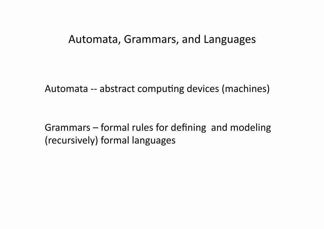
Automata, Grammars, and Languages

Automata -‐-‐ abstract compuBng devices (machines)

Grammars – formal rules for defining and modeling (recursively) formal languages

Finite State Machine

Example 1

M 001100 11bbbb

Replace prefix 0’s by 1’s, and each remaining symbol by b

0/1 0/b, 1/b

1/b

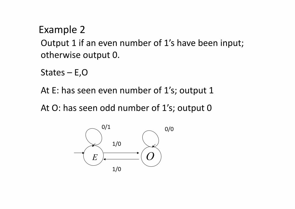
Example 2 Output 1 if an even number of 1’s have been input; otherwise output 0.

States – E,O

At E: has seen even number of 1’s; output 1

At O: has seen odd number of 1’s; output 0

0/1 0/0

1/0

1/0

Finite State Automata

€

Similar to finite state machines, without output functions, with designated initial state and accepting states.

M = (I,S, f ,A,σ)I : finite set of input symbolsS : finite set of statesf : S × I→S next - state function (state transition)A ⊂ S : accepting statesσ : initial state

Example

b b

a a

a,b

a

M: Accept strings over {a,b} with exactly two a’s.

b

FA as language recognizers

Example

Accept bit strings that contain 101 as a substring.

0 1

1

0

0 1

0,1

A simple example of grammar

DefiniBon of Grammar

€

A grammar G consists ofA finite set N of nonterminal symbolsA finite set T of terminal symbols where N ∩T =∅

A finite set P of production rules of the form A→Bwhere A is a string over N ∪T with at least one nonterminal symbol, and B is a string over N ∪T.

Language of a Formal Grammar

The language of a formal grammar G = (N, Σ, P, S), denoted as L(G), is defined as all those strings over Σ that can be generated by starting with the start symbol S and then applying the production rules in P until no more non-terminal symbols are present.

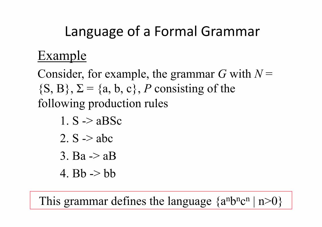
Language of a Formal Grammar

Example Consider, for example, the grammar G with N = {S, B}, Σ = {a, b, c}, P consisting of the following production rules

1. S -> aBSc 2. S -> abc 3. Ba -> aB 4. Bb -> bb

This grammar defines the language {anbncn | n>0}

Chomsky's four types of grammars •  Type-‐0 grammars (unrestricted grammars) languages recognized by a Turing machine

•  Type-‐1 grammars (context-‐sensiBve grammars)

Turing machine with bounded tape

•  Type-‐2 grammars (context-‐free grammars)

pushdown automaton

•  Type-‐3 grammars (regular grammars)

regular expressions, finite state automaton

Musical Grammars

•  BOL Processor: (regular) – Example of Tabla Drumming as paeern language

•  Steedman Jazz Grammar (context free)

•  GTTM (unrestricted)

Cellular Automata

Dynamic system specified by iniBal condiBon and a set of evoluBon rules

Cellular Automata

•  Discrete Dynamical System – Space and Bme

•  Dimension – 1-‐D, 2-‐D, …

•  States – Neighborhood and neighbors

•  Rules

31

1-‐D Cellular Automata

•  Neighborhood

32


•  Black & White neighbors (States)

•  Neighborhood

33



•  Neighborhood

•  Rules

34



•  Neighborhood

•  Rules

•  Example

t = 1

35



•  Neighborhood

•  Rules

•  Example

t = 1 t = 2

36



•  Neighborhood

•  Rules

•  Example

t = 1 t = 2

37



•  Neighborhood

•  Rules

•  Example

t = 1 t = 2

38



•  Neighborhood

•  Rules

•  Example

t = 1 t = 2

39



•  Neighborhood

•  Rules

•  Example

t = 1 t = 2

40

Wolfram Code Every cell and its two neighbors will be one of the following types

Represent a black cell with 1 and a white cell with 0

1 1 1 1 1 0 1 0 1 1 0 0 0 1 1 0 1 0 0 0 1 0 0 0

Every yellow cell above can be filled out with a 0 or a 1 giving a total of 2 8=256 possible update rules.

This allows any string of eight 0s and 1’s to represent a disBnct update rule

Example: Consider the string 0 1 1 0 1 0 1 0 it can be taken

to represent the update rule

1 1 1 1 1 0 1 0 1 1 0 0 0 1 1 0 1 0 0 0 1 0 0 0 0 1 1 0 1 0 1 0

Or equivalently

Now think of 01101010 as the binary expansion of the number

0 27+ 1 26+ 1 25+ 0 24+1 23+ 0 22+ 1 21+ 0 20 = 64+32+8+2=106.

So the update rule is rule # 106

Rule #45=32+8+4+1

= 0 27+ 0 26+ 1 25+ 0 24+1 23+ 1 22+ 0 21+ 1 20 =0 0 1 0 1 1 0 1

Rule #30=16+8+4+2

= 0 27+ 0 26+ 0 25+ 1 24+1 23+ 1 22+ 1 21+ 0 20 =0 0 0 1 1 1 1 0

This is a naming convenBon of the 256 disBnct update rules by Stephen Wolfram, New Kind of Science.

Notable rules in this class include rule 30, rule 110, and rule 184. Rule 90 is also interesBng because it creates Pascal's Triangle modulo 2.

Rule 110 is known to be Turing complete. This implies that, in principle, any calculaBon or computer program can be simulated using this automaton.

hep://en.wikipedia.org/wiki/Elementary_cellular_automaton

Rule 30

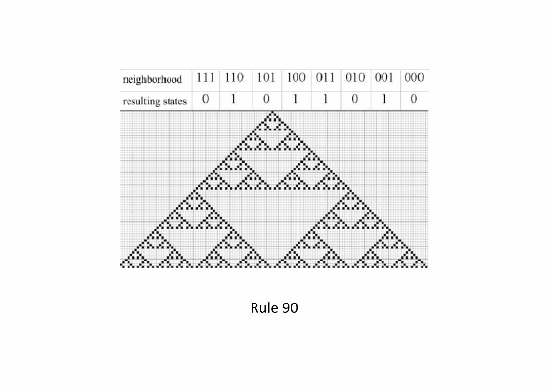
Rule 90

Classes of cellular automata (Wolfram)

Class 1: arer a finite number of Bme steps, the CA tends to achieve a unique state from nearly all possible starBng condiBons (limit points)

Class 2: the CA creates paeerns that repeat periodically or are stable (limit cycles) – probably equivalent to a regular grammar/finite state automaton

Class 3: from nearly all starBng condiBons, the CA leads to aperiodic-‐chaoBc paeerns, where the staBsBcal properBes of these paeerns are almost idenBcal (arer a sufficient period of Bme) to the starBng paeerns (self-‐similar fractal curves) – computes ‘irregular problems’

Class 4: arer a finite number of steps, the CA usually dies, but there are a few stable (periodic) paeerns possible (e.g. Game of Life) -‐ Class 4 CA are believed to be capable of universal computaBon

improvisation - lecture 1

Documents