in-band spectrum sensing in cognitive radio networks ... · in-band spectrum sensing in cognitive...

In-band Spectrum Sensing in Cognitive Radio Networks:Energy Detection or Feature Detection?

Hyoil Kim and Kang G. ShinReal-Time Computing Laboratory, EECS Department

The University of Michigan, Ann Arbor, MI 48109-2121, USA.{hyoilkim, kgshin}@eecs.umich.edu

ABSTRACTIn a cognitive radio network (CRN), in-band spectrum sens-ing is essential for the protection of legacy spectrum users,with which the presence of primary users (PUs) can be de-tected promptly, allowing secondary users (SUs) to vacatethe channels immediately. For in-band sensing, it is impor-tant to meet the detectability requirements, such as the max-imum allowed latency of detection (e.g., 2 seconds in IEEE802.22) and the probability of mis-detection and false-alarm.In this paper, we propose an efficient periodic in-band sens-ing algorithm that optimizes sensing-frequency and sensing-time by minimizing sensing overhead while meeting the de-tectability requirements. The proposed scheme determinesthe better of energy or feature detection that incurs lesssensing overhead at each SNR level, and derives the thresh-old aRSSthreshold on the average received signal strength(RSS) of a primary signal below which feature detection ispreferred. We showed that energy detection under lognor-mal shadowing could still perform well at the average SNR< SNRwall [1] when collaborative sensing is used for its lo-cation diversity. Two key factors affecting detection perfor-mance are also considered: noise uncertainty and inter-CRNinterference. aRSSthreshold appears to lie between −114.6dBm and -109.9 dBm with the noise uncertainty rangingfrom 0.5 dB to 2 dB, and between −112.9 dBm and −110.5dBm with 1∼6 interfering CRNs.

Categories and Subject DescriptorsC.2.1 [Computer-Communication Networks]: NetworkArchitecture and Design—Wireless communication

General TermsAlgorithms, Design, Performance, Theory

KeywordsSpectrum sensing and opportunity, sensor clustering, sens-ing scheduling, energy and feature detection

Permission to make digital or hard copies of all or part of this work forpersonal or classroom use is granted without fee provided that copies arenot made or distributed for profit or commercial advantage and that copiesbear this notice and the full citation on the first page. To copy otherwise, torepublish, to post on servers or to redistribute to lists, requires prior specificpermission and/or a fee.MobiCom’08, September 14–19, 2008, San Francisco, California, USA.Copyright 2008 ACM 978-1-60558-096-8/08/09 ...$5.00.

1. INTRODUCTIONCognitive radio (CR) is a key technology for alleviating

the inefficient spectrum-utilization problem under the cur-rent static spectrum-allocation policy [2–4]. In cognitivenetworks (CRNs), unlicensed or secondary users (SUs) areallowed to opportunistically utilize spectrum bands assignedto licensed or primary users (PUs) as long as they do notcause any harmful interference to PUs. A spectrum oppor-tunity refers to a time duration on a channel1 during whichthe channel can be used by SUs without interfering with thechannel’s PUs. In-band channels refer to those channels cur-rently in use by SUs; all others are referred to as out-of-bandchannels.

One of the major challenges in CRNs is to strike a bal-ance between (1) protection of PUs against interference fromSUs and (2) efficient reuse of legacy spectrum, for whichspectrum sensing is essential. That is, spectrum sensing dis-covers spectrum opportunities or holes by monitoring out-of-band channels and detecting white spaces [5]. When thus-discovered opportunities are utilized by SUs, in-band spec-trum sensing must promptly detect return of PUs to an in-band channel so that SUs can vacate the channel immedi-ately upon detection of returning PUs.

For maximal protection of PUs, FCC has set a strictguideline on in-band sensing. For example, in IEEE 802.22,the world’s first international CR standard,2 PUs shouldbe detected within 2 seconds of their appearance with theprobability of misdetection (PMD) and the probability offalse detection (PFA) less than 0.1. To meet these require-ments, in-band sensing must be run frequently enough (atleast once every 2 seconds) and a detection method (e.g.,energy and feature detection [6]) that yields the best per-formance should be selected. Both the sensing frequencyand the detection method should be chosen by consideringthe impact on SUs’ QoS impairment since sensing should beperformed during quiet periods [6, 7], i.e., communicationsbetween SUs are suspended.

This paper presents an efficient in-band sensing algorithmthat (1) derives the period of sensing by minimizing theamount of sensing time, or sensing overhead, while meet-ing the detectability requirement, and (2) selects the de-tection method that incurs less sensing overhead. In whatfollows, we first advocate use of clustered sensor networksto support in-band spectrum sensing, identifying two im-

1Spectrum band and channel will be used interchangeablyin this paper.2Note that IEEE 802.22 is still a draft at the time of thiswriting.

portant research challenges. Second, we show how appro-priate scheduling of in-band sensing can enhance the sens-ing performance and help support QoS in CRNs. We alsoshow that SNRwall [1] of energy detection, which acts asan absolute barrier in an AWGN channel, is breakable in ashadow-fading channel when the average SNR of collabora-tive sensors is less than SNRwall. Based on this finding,energy detection is preferred to feature detection even at avery small SNR.

1.1 Sensor Clustering

1.1.1 MotivationCollaborative sensing [8–10] is known to be essential for

better detectability as it exploits sensor diversity via simul-taneous sensing on a channel at multiple locations. Presenceof PUs on a channel is determined by processing the mea-surements via data fusion. A common data fusion rule is theOR-rule [11] where PUs are considered present if at least onesensor reports their presence. Its sensing performance withN cooperative sensors has been shown as

PMD(N) = PMDN , and PFA(N) = 1− (1− PFA)N , (1)

under the assumption that every sensor has the same PMD

and PFA for a given signal.Eq. (1), however, does not hold in a large CRN such as an

IEEE 802.22 network in which a base station (BS) covers anarea of radius ranging from 33 km (typical) to 100 km [6].In such a case, the average received signal strength (RSS)3

of a primary signal at two distant sensor locations (CPE Aand CPE B in Fig. 1) may vary significantly. HeterogeneousPMD and PFA of each sensor must therefore be consideredin modeling collaborative sensing performance, making itharder to design a collaborative sensor network (e.g., deter-mining the number of cooperative sensors needed).

Sensor clustering avoids this problem by grouping sensorsin close proximity into a cluster so that they can measure asimilar average RSS of any primary signal. Sensor clusteringalso mitigates the control overhead in data fusion. Insteadof forcing all sensors to report their measurements to theBS, each cluster head (CH) can collect intra-cluster mea-surements and make a local decision, which is then reportedto the BS.

1.1.2 ContributionsAlthough there has been considerable research into clus-

tered CR sensor networks [13–15], two important issues havenot yet been addressed: (1) cluster size and (2) sensor den-sity. Section 3 addresses these two issues as follows. First,we will derive the maximum radius of a cluster so as toupper-bound the variation of the average RSS in a clusterby 1 dB. Second, we will derive the maximum sensor densityto guarantee near-independent sensor observations. Mishraet al. [16] claimed that 10–20 independent sensors performbetter than many more correlated sensors since correlationbetween sensors due to shadow fading limits the collabora-tive sensing gain. Since the correlation between two sensorsdecreases exponentially as distance between sensors growslinearly [17], we can upper-bound sensor density such that

3Note that the “average” received singal strength (aRSS)is the empirical large-scale path loss of the shadow fadingmodel introduced in [12].

the average distance between neighboring sensors is lower-bounded and the shadow correlation is smaller than 0.3.

With this approach, one-time (collaborative) in-band sens-ing in a cluster can be completely described by Eq. (1) whereN now becomes the number of cooperative sensors withina cluster. Next, we consider periodic scheduling of in-bandsensing and its related issues.

1.2 Scheduling of In-band Sensing

1.2.1 MotivationIEEE 802.22 requires in-band sensing to achieve PMD ≤

0.1 in detecting the presence of primary signals within achannel detection latency threshold CDT which is typically2 seconds. PFA is interpreted similarly: PFA ≤ 0.1 shouldbe achieved if the sensing algorithm runs for CDT secondswhen no PUs are present.

IEEE 802.22 also provides the two-stage sensing (TSS)mechanism where a sensing algorithm can decide which ofenergy or feature detection is used in a quiet period. Al-though energy detection incurs minimal time overhead (usu-ally less than 1 ms), its susceptibility to noise uncertainty [1]limits its usability. Feature detection is less susceptible tonoise uncertainty [18] but it requires a longer sensing time(e.g., 24.2 ms for the field sync detector [6]).

The current IEEE 802.22 draft does not specify how oftensensing must be scheduled and which detection method touse, and under what condition. Although there have beenseveral studies on the performance of energy and feature de-tection [6,19–23], they were all based on one-time detection.Hence, we propose an efficient sensing algorithm that (1)minimizes sensing overhead by optimizing the sensing pe-riod (TP in Fig. 2) and the sensing time (TI in Fig. 2), and(2) chooses the better of energy or feature detection in agiven sensing environment.

1.2.2 ContributionsSNRwall [1] implies the minimum SNR threshold due to

noise uncertainty below which a detector cannot reliablyidentify a primary signal, regardless of how much time ittakes. SNRwall of energy detection is often understood asan absolute barrier, and hence, energy detection completelyfails at a very low SNR. However, we will show that SNRwall

is an absolute barrier only in the AWGN channel, and in re-ality, the barrier becomes obscure with the shadowing chan-nel. As a result, in most cases energy detection is still a goodcandidate for sensing because of its low sensing-time. Thatis, although feature detection may perform better than en-ergy detection with one-time sensing, energy detection canoutperform feature detection by sensing more frequently.

Two important factors affecting the detection performance—noise uncertainty and inter-CRN interference—will also beinvestigated and their effects will be evaluated extensively.We will finally propose a sensing strategy to decide the bestdetection method for a given sensing condition.

1.3 Related WorkThere have been continuing discussions on using clustered

networks in CRs. Chen et al. [13] proposed a mechanism toform a cluster among neighboring nodes and then intercon-nect such clusters. Pawelczak et al. [15] proposed cluster-based sensor networks to reduce the latency in reportingsensor measurements by designating the cluster head as a

TV transmitter

150.3 km (keep-out radius)

BS

33 km (typical)

CPEsCPE A

CPE B

Figure 1: Illustration of an IEEE 802.22 cell whichcoexists with a TV transmitter.

local decision maker. Sun et al. [14] enhanced performanceby clustering sensors where the benefit comes from clusterand sensor diversities. None of these authors, however, men-tioned the importance of optimizing cluster size and sensordensity.

Despite extensive existing studies on the performance ofone-time signal detection in CRs, the optimal scheduling ofin-band sensing has been received far less attention. Cordeiroet al. [6] evaluated the performance of fast sensing in 802.22by scheduling fast sensing (1 ms) every 40 ms, but theydid not optimize the sensing-time and sensing-period (orequivalently, sensing-frequency). Datla et al. [24] proposed abackoff-based sensing scheduling algorithm, but their schemewas not designed for detecting returning PUs in an in-bandchannel. Hoang and Liang [25] introduced an adaptive sens-ing scheduling method to capture the tradeoff between SUs’data-transmission and spectrum-sensing. Their scheme, how-ever, did not focus on in-band sensing for protection of PUs.

1.4 OrganizationSection 2 briefly reviews IEEE 802.22, followed by a sum-

mary of spectrum sensing including fine/fast sensing details.In Section 3, we first introduce the concept of sensor clus-tering, and then derive the maximum radius of a cluster aswell as the maximum sensor density. Section 4 describes theproposed in-band sensing algorithm that can be used in acluster. We consider two factors in building the algorithm:(1) noise uncertainty and (2) existence of interfering sec-ondary networks (SNs). The performance of the proposedin-band sensing algorithms is evaluated in Section 5, and thepaper concludes in Section 6.

2. PRELIMINARIES

2.1 IEEE 802.22In this paper, we consider the scheduling of in-band sens-

ing in an IEEE 802.22 network. Note, however, that ourproposed schemes can be applied to future CR standardswith no/slight modifications.

The IEEE 802.22 network is an infrastructure-based wire-less network where a Base Station (BS) coordinates nodes ina single-hop cell which covers an area of radius ranging from33 km (typical) to 100 km. End-users of an 802.22 cell arecalled Consumer Premise Equipments (CPEs) representinghouseholds in a rural area (and hence stationary nodes).

802.22 reuses UHF/VHF bands where three types of pri-mary signals present: Analog TV, Digital TV, and wirelessmicrophones. Our proposed schemes in this paper consider

sensing-time (TI)

ON

OFF

“busy” “idle”samples

sensing

“idle” “idle” “busy”

sensing-period (TP)

sensing-frequency = 1 / TP

Figure 2: The ON/OFF channel model and periodicsensing process with sensing-period TP and sensing-time TI

DTV transmitters as the major source of primary transmis-sion; their extension for wireless microphones is part of ourfuture work. By considering the minimum D/U (Desired toUndesired) signal ratio of 23 dB and the DTV protectioncontour of 134.2 km, the keep-out radius of CPEs from theDTV transmitter is given as 150.3 km [19]. CPEs within thiskeep-out radius are forced to avoid use of the DTV channel.Fig. 1 illustrates this scenario.

2.2 Channel and Sensing ModelA channel is modeled as an ON/OFF source, where an

ON period represents the time duration during which PUsare actively using their channel. SUs are allowed to utilizethe channel only during PUs’ OFF periods. This model hasbeen used successfully in modeling the PUs’ channel-usagepattern in many applications [26–28]. A TV transmitter’schannel usage pattern usually has very long (in the order ofhours) ON and OFF periods.

Spectrum sensing is akin to sampling in that it measures achannel’s state during the sensing time (denoted as TI) anddetects the presence of PU signals at that moment. TI mayvary with detection methods (e.g., less than 1 ms for energydetection). Fig. 2 illustrates the ON/OFF channel modeland an example periodic sensing process with sensing-timeTI and sensing-period TP .

In 802.22, sensing must be performed during a quiet pe-riod within which no CPEs are allowed to transmit data sothat any signal activity detected by sensors should originatefrom the PUs. The quiet periods have to be synchronizedamong sensors in the same cell as well as between neigh-boring cells, which is achieved by the Coexistence BeaconProtocol (CBP) via exchange of CBP frames [6].

2.3 Signal Detection MethodsWe briefly overview the detection methods used in IEEE

802.22, along with their theoretical performance in terms ofPMD and PFA.

2.3.1 Energy DetectionEnergy detection is the most popular for signal detection

due to its simple design and small sensing time. Shellham-mer et al. [19] analyzed the energy detection of a DTV signalusing its discrete-time samples, where the signal is sampledby its Nyquist rate of 6 MHz.4 The detection threshold γ to

4The DTV signal ranges from -3 MHz to +3 MHz in thebaseband.

yield PFA is given as

γ = NdB

(1 +

Q−1(PFA)√M

), (2)

and PMD with γ is given as

PMD = Q

( √M

P + NdB[(P + NdB)− γ]

). (3)

where M is the number of samples, Nd the noise power spec-tral density (PSD), B the signal bandwidth (6 MHz), P thesignal power, and Q(·) the Q function.

Note that the effect of multipath fading is insignificant indetecting a DTV signal due to frequency diversity over the6 MHz band [18, 19]. Instead, the impact of shadow fadingmust be considered in the variation of RSS at different sen-sor locations. Ghasemi and Sousa [10] derived the averageperformance of energy detection by numerically integratingPMD over the fading statistics.

2.3.2 Feature DetectionFeature detection captures a specific signature of a DTV

signal, such as pilot, field sync, segment sync, or cyclosta-tionarity [6]. Each feature detector is reviewed briefly forcompleteness.

ATSC uses 8-VSB to modulate a DTV signal, and an off-set of 1.25 is added to the signal which creates a pilot signalat a specific frequency location. The authors of [21] intro-duced pilot energy detection which filters the DTV signalwith a 10 KHz narrowband filter at the pilot’s frequencylocation. They showed that the pilot signal’s SNR is 17dB higher than the DTV signal’s SNR, making the pilot astrong feature to detect.

A DTV data segment starts with a data segment sync ofpattern {+5 -5 -5 +5}. A data field consists of 313 datasegments, and the first data segment of each data field iscalled a field sync segment which contains special pseudo-random sequences: PN511 and PN63. Therefore, segmentsync and field sync can be used as a unique feature of DTVsignal. Detectors of such features are introduced by manyresearchers, such as [6,13,29,30], but no analytical derivationof PMD and PFA has been reported, i.e., they were evaluatedonly via simulation.

Since the DTV signal is digitally modulated, it shows thecyclostationary feature. Recently, Goh et al. [23], Han et al.[31], and Chen et al. [13] studied cyclostationary detection ofATSC and DVB-T DTV signals and investigated its perfor-mance via simulation, since the derivation of PMD/PFA ofcyclostationary detectors for complex modulation schemes(e.g., 8-VSB) are known to be mathematically intractable[32].

In this paper, we choose the pilot energy detector amongfeature detectors for an illustrative purpose and use it toevaluate the tradeoffs between energy and feature detection,since its performance has been mathematically analyzed in[21]. Other types of feature detection, however, can also beused for our proposed method in Section 4 by evaluatingPMD and PFA via simulation at a detection threshold weare interested in, for which the real DTV signal capturedata in [33] and the sensing simulation model in [34] can beutilized.

PMD and PFA of the pilot energy detector (will hence-forth be called simply “pilot detector”) are derived similarlyto energy detection and well described in [21]. Shellhammer

BS

CPEs

Sensor

cluster

Additional

sensor

BSCluster

head

802.22 cell

Figure 3: An illustration of clustered sensor net-works in an IEEE 802.22 cell

and Tandra [21] stated that the pilot signal’s SNR may bedegraded due to both uncertainty in the pilot locations over59 KHz and inaccuracy in the local oscillator (LO) of the lowpass filter, which forces the detector to use a 70 KHz band-pass filter. Therefore, we will use the sampling frequency of70 KHz, instead of 10 KHz, in our analysis. Unlike energydetection in a 6 MHz bandwidth, Rayleigh fading becomesa significant factor, as it is flat in the narrow band of 70KHz. Hence, we will consider both Rayleigh and lognormalshadow fading in deriving PMD and PFA of pilot detection.

3. SPECTRUM SENSOR CLUSTERINGAs discussed in Section 1, the performance of collaborative

sensing can be enhanced by clustering sensors in the networkto make the gain of collaborative sensing more predictable.Sensor clustering can also make a sensor network scalable incollecting measurements for data fusion by enabling clusterheads (CHs) to make local decisions. The concept of a 2-tiered sensor cluster network is illustrated in Fig. 3.

We identify two important challenges in sensor clustering:cluster size and sensor density.

3.1 Cluster SizeWe will derive the maximum radius of a sensor cluster

so that the variation of average RSS within a cluster willbe bounded by 1 dB, to make it possible to use Eq. (1)in modeling the performance of a collaborative sensor net-work. The effect of fading is considered by averaging PMD

of Eq. (3) over the fading statistics (Rayleigh fading or log-normal shadowing) and by substituting the result in Eq. (1).

According to the path-loss model of polynomial power de-cay [35], the average RSS at a sensor r meters away from aprimary transmitter (PT) is given as P1r

−α12 , where P1 isthe PT’s transmit power and α12 is the path loss exponent.The maximum variation of the average RSS in a cluster isfound between two sensors located at (R − Rcluster) and(R+Rcluster) meters away from the PT, respectively, whereR is the distance between the PT and the center of a clus-ter, and Rcluster is the radius of a cluster. Therefore, themaximum cluster size is determined as

10α12log10

(R + Rcluster

R−Rcluster

)≤ 1(dB),

23

4d

Figure 4: An example hexagonal deployment ofspectrum sensors

which gives

Rcluster =β − 1

β + 1R, β = 100.1/α12 .

For example, for a cluster at the keep-out radius of 150.3km (i.e., R = 150.3 km), Rcluster is given as 5.76 km, usingα12 = 3 suggested in the Hata model [36–38].5

3.2 Sensor DensityMishra et al. [16] claimed that a few tens of independent

sensors provide as much collaborative gain as many morecorrelated sensors whose collaborative gain is limited bygeographical correlation in shadowing. According to Gud-mundson’s model [17], the shadow correlation decays expo-nentially as distance between two locations increases. As aresult, a blind increase in sensor density does not yield a lin-ear increase of collaborative gain. Therefore, we will explorethe maximum sensor density to guarantee enough distancebetween sensors for near-independent observations. We willalso show that the minimum sensor density provides a suffi-cient number of minimally-correlated sensors in a cluster.

The shadow correlation between two locations that ared meters apart is given as R(d) = e−ad, a = 0.002, in asuburban area [11,17]. We want to suppress the correlationto be, on average, less than 0.3 between any two neighboringsensors. That is, R(d) = e−0.002d ≤ 0.3, which gives d ≥ 602m.

Assuming the hexagonal deployment of sensors as shownin Fig. 4, where the minimum distance between neighbors isd, the density of sensors (DS) is shown to be

DS =2√3d2

(sensors/m2),

and hence for d = 602 m, the maximum sensor density is

DmaxS = 3.18(sensors/km2).

The minimum sensor density (DminS ) is determined by the

household density, since a household represents a CPE which

5Although the Hata model is not the best fit for 802.22 sinceit is designed to describe power decay of the transmittedsignal up to 20 km from the PT, it works better than thewidely-accepted Okumura model [39] which does not dealwith rural environments. In this paper, we consider α12 asa design parameter and evaluate our schemes with α12 = 3as an example. Determination of α12 is outside of the scopeof this paper.

Analog TV (NTSC) -94 dBm (at peak of sync ofthe NTSC picture carrier)

Wireless Microphones -107 dBm (200 KHz bandwidth)Digital TV (ATSC) -116 dBm (6 MHz bandwidth)

Table 1: Incumbent detection threshold (IDT ) ofprimary signals

plays role as both a sensor and a transceiver. According tothe WRAN reference model [40], the minimum householddensity in a rural area is 0.6 (houses/km2). Therefore, theminimum sensor density is

DminS = 0.6(sensors/km2).

The next question is: at DminS , are there enough (i.e., at

least 10 or more) sensors in a cluster for collaboration? Us-ing the above-derived Dmin

S and DmaxS , the number of sen-

sors in a cluster ranges between Nminsensor and Nmax

sensor where

Nminsensor = Dmin

S · πRcluster2,

Nmaxsensor = Dmax

S · πRcluster2.

With Rcluster = 5.76km, this gives 62∼331 sensors per clus-ter which exceeds the recommendation in [16]. Therefore,the CH can select a subset of sensors for each quiet periodin such a way that its area can be covered evenly.

3.3 DiscussionIn a real deployment scenario, the location of CPEs is not

determined by the hexagonal model, since they are likelyto be cluttered within small areas (e.g., a town or a vil-lage) where the actual sensor density is much higher thanthe average household density (e.g., 0.6 houses/km2). Onthe other hand, CPEs are rare outside the populated areas.Therefore, we take two approaches: (1) the CHs in a popu-lated area should selectively choose CPEs according to therecommended sensor density to avoid correlated measure-ments, and (2) the wireless service provider (WSP) has todeploy additional sensors in less-populated areas to achieveDmin

S (as shown in Fig. 3). In either case, the hexagonalmodel may be still useful in determining the proper loca-tions of CPEs to be selected or sensors to be deployed.

A sensor cluster may be further divided into smaller sub-clusters to detect localized deep shadow fading which is notrepresented well by the lognormal shadowing model. In thiscase, sensors more than Nmax

sensor can be elected in each clus-ter so that their correlated measurements can be used toidentify any localized shadowing. Further development ofsub-clustering may be possible, but it is left as our futurework.

4. SCHEDULING OF IN-BAND SENSING

4.1 Sensing Requirements in IEEE 802.22We briefly overview the sensing requirements in IEEE

802.22. Incumbent detection threshold (IDT ) is the weakestprimary signal power (in dBm) above which sensors shouldbe able to detect. IDT s for three types of primary signals(in the US) [7] are shown in Table 1. As mentioned earlier,we will focus on DTV signals.

Channel detection time (CDT ) is given to be ≤2 sec-onds, within which the returning PUs must be detected with

PMD ≤ 0.1, regardless of the number of times sensing is per-formed during CDT . Similarly, PFA ≤ 0.1 must also be metwhen the same sensing algorithm used to meet PMD ≤ 0.1is run for CDT seconds during which no PUs are present.The requirement on PMD is to guarantee minimal interfer-ence to incumbents, whereas the requirement on PFA is toavoid unnecessary channel switching due to false detectionof PUs.

Based on the above interpretation of PMD and PFA, thetwo performance metrics can be expressed as

PMD = Pr(detect PT within CDT | H1) ≤ 0.1,

PFA = Pr(detect PT within CDT | H0) ≤ 0.1, (4)

where H0 and H1 are two hypotheses on the presence of PUsin the channel:

H0 : No PU exists in the channel,

H1 : PUs exist in the channel.

Note that PMD and PFA in Eq. (4) have different mean-ings from those in Eq. (1). PMD and PFA in Eq. (4) are theprobabilities measured by monitoring an in-band channelfor CDT seconds during which sensing may be scheduledmultiple times, whereas PMD and PFA in Eq. (1) are theprobabilities of one-time sensing. To avoid any confusion,we will henceforth replace PMD and PFA in Eq. (4) withP CDT

MD and P CDTFA .

4.2 TSS mechanism in IEEE 802.22To support a sensing algorithm to meet the detectability

requirements shown in Eq. (4), IEEE 802.22 provides thetwo-stage sensing (TSS) mechanism. With TSS, a sensingalgorithm schedules either fast or fine sensing in each quietperiod (QP), where fast sensing employs energy detectionwhile fine sensing uses feature detection.

Although a sensing algorithm can schedule as many QPsas it wants, there are some restrictions on the sensing period.For example, the QP of fast sensing, usually less than 1 ms,should be scheduled at the end of an 802.22 MAC frame (10ms) at most once in each frame. Hence, the period of fastsensing becomes a multiple of the frame size (i.e., n · 10 ms,n: positive integer). On the other hand, the QP duration offine sensing varies with the feature detection scheme used.In case the feature-detection scheme requires the sensing-time longer than one MAC frame (e.g., 24.2 ms for DTV fieldsync detection), its QP should be scheduled over consecutiveMAC frames.

4.3 In-band Sensing Scheduling AlgorithmAn efficient sensing algorithm must capture the tradeoff

between fast and fine sensing: for one-time sensing, (1) fastsensing consumes a minimum amount of time but its per-formance is more susceptible to noise uncertainty and co-channel interference, and (2) fine sensing usually requiresmuch more time than fast sensing, but its performance isbetter than fast sensing. Therefore, the sensing algorithmmay have to schedule fast sensing at a high frequency, orit may decide to schedule fine sensing at a lower frequency.In either case, the scheduling goal is to minimize the over-all time spent for sensing (or the sensing-overhead) whilemeeting the detectability requirements.

ON

OFF

τ

CDT

PT

# sensing = 1 −

+ P

CDT

T

τ

sensing

… …

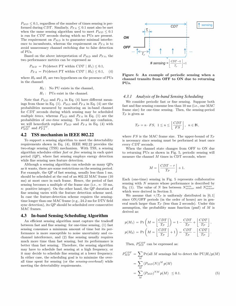
Figure 5: An example of periodic sensing when achannel transits from OFF to ON due to returningPUs.

4.3.1 Analysis of In-band Sensing SchedulingWe consider periodic fast or fine sensing. Suppose both

fast and fine sensing consume less than 10 ms (i.e., one MACframe size) for one-time sensing. Then, the sensing-periodTP is given as

TP = n · FS, 1 ≤ n ≤⌊

CDT

FS

⌋, n ∈ N,

where FS is the MAC frame size. The upper-bound of TP

is necessary since sensing must be performed at least onceevery CDT seconds.

When the channel state changes from OFF to ON dueto returning PUs as shown in Fig. 5, periodic sensing willmeasure the channel M times in CDT seconds, where

M =

⌊CDT − τ

TP

⌋+ 1.

Each (one-time) sensing in Fig. 5 represents collaborativesensing with N sensors whose performance is described byEq. (1). The value of N lies between Nmin

sensor and Nmaxsensor

which were derived in Section 3.We assume that τ/TP is uniformly distributed in [0, 1]

since ON/OFF periods (in the order of hours) are in gen-eral much larger than TP (less than 2 seconds). Under thisassumption, the probability mass function (pmf) of M isderived as:

p(M1) = Pr

(M =

⌊CDT

TP

⌋)= 1− CDT

TP+

⌊CDT

TP

⌋,

p(M2) = Pr

(M =

⌊CDT

TP

⌋+ 1

)=

CDT

TP−

⌊CDT

TP

⌋.

Then, P CDTMD can be expressed as:

P CDTMD =

∑M

Pr(all M sensings fail to detect the PU|H1)p(M)

=∑M

(PMD(N))M p(M)

=∑M

(PMD)NM p(M) ≤ 0.1. (5)

Similarly, P CDTFA can be expressed as:

P CDTFA = 1−

∑M

Pr(none of M sensings detects PUs|H0)p(M)

= 1−∑M

(1− PFA(N))M p(M)

= 1−∑M

(1− PFA)NM p(M) ≤ 0.1. (6)

In Eqs. (5) and (6), PMD and PFA are detection-methodspecific. They also depend on the sensing-time (TI) and theRSS of the primary signal. PMD and PFA of energy andpilot detectors are fully described by Eqs. (2) and (3).

4.3.2 The Proposed Sensing Scheduling AlgorithmOur objective is to find the optimal sensing-period TP for

given TI and RSS, that minimizes the sensing overhead whilesatisfying two conditions of Eqs. (5) and (6). The sensing-overhead of a sensing algorithm is defined as the fraction oftime in which sensing is performed. That is,

sensing-overhead =TI

TP

for periodic sensing.The problem of optimizing TP is identical to that of max-

imizing n that satisfies Eqs. (5) and (6). Therefore, the pro-posed algorithm examines n from its upper bound bCDT/FScand decreases n until the one that meets the condition isfound.

Since P CDTFA is a monotonic function6 of PFA and there

is a one-to-one mapping between PFA and PMD, we firstwant to find the value of PFA that solves the equality ofEq. (6). Then, PMD corresponding to PFA can be foundfrom the ROC curve between them. Finally, the feasibilityof the tested n can be checked by substituting PMD intoEq. (5). If the tested n does not satisfy Eq. (5), then n isdecreased by 1 and the above procedure is repeated.

If there does not exist any n satisfying both equations, thedetection method considered cannot meet the detectabilityrequirements with given TI and RSS. On the contrary, ifthe optimal sensing period is found at n = nopt, its sensingoverhead is determined as: TI/(nopt · FS).

The pseudo-code of the proposed algorithm for energy andpilot detection is given in Fig. 6.

4.3.3 Implementation IssuesAn important aspect of the proposed algorithm is that it

computes the optimal sensing periods offline, and the opti-mal periods can be looked up from the database with twoinputs, TI and RSS, at runtime. A sensor can create/storeone database per detection method, and adaptively choosethe best method with optimal TP and TI .

Note that PMD and PFA of a single sensor to meet Eqs. (5)and (6) are functions of N . This suggests that IEEE 802.22may need to refine its definition/requirement on PMD andPFA so that they can be determined adaptively taking N asa variable.

In Section 5, we will evaluate and compare the perfor-mance of energy and pilot detection. The optimal sensingstrategy (i.e., optimal detection, period, and time) with the

6One can easily show this by differentiating P CDTFA with re-

spect to PFA.

n := bCDT/FSc;

while (n > 0) {PFA := {x|1−∑

M (1− x)NM p(M) = 0.1};γ := NdB(1 + Q−1(PFA)/

√M);

PMD := Q([(P + NdB)− γ] · √M/(P + NdB));if (P CDT

MD (PMD) ≤ 0.1) then {〈set sensing-period: TP = n · FS〉;return;

}else n := n− 1;

}〈mark the current detection method infeasible〉;return;

Figure 6: Pseudo-code of the in-band sensingscheduling algorithm

average RSS varying from −120 dBm to −90 dBm will alsobe proposed.

5. PERFORMANCE EVALUATION

5.1 Two Important Factors in In-band Sens-ing

5.1.1 Noise UncertaintyBelow a certain SNR threshold, called SNRwall [1], energy

detection in the AWGN channel is found to completely failto detect a signal irrespective of the amount of sensing-timeused. SNRwall results from the uncertainty in the noisepower (called noise uncertainty), and their relationship isgiven as

SNRwall =ρ2 − 1

ρ,

when ρ = 10x/10 and x is the noise uncertainty in dB. In [41],the amount of noise uncertainty is shown to depend on fourfactors: calibration error, thermal variation, changes in low-noise amplifier (LNA) gain, and interference, where the noiseuncertainty under 20 ◦K of temperature variation is givenas ±1 dB.

Based on this finding, energy detection is often consideredunsuitable for CRNs which must detect very weak signalpower (e.g., as low as −116 dBm for DTV signals). How-ever, we found that SNRwall can actually be overcome evenwhen the average SNR (by the aRSS) is less than SNRwall,via the location diversity of collaborative sensing. AlthoughSNRwall plays role as an absolute barrier when the AWGNchannel is considered, the energy detection of DTV sig-nals will experience a lognormal shadow-fading channel withwhich SNRwall becomes penetrable because at some sensorlocations instantaneous SNR may exceed SNRwall even ifthe average SNR in the sensor network is below the wall.

The effect of shadow-fading can be clearly observed inFigs. 7 and 8, where dB-spread of 5.5 dB [34] is used forshadow-fading. In general, the performance under shadow-fading channel is worse than the AWGN channel. However,from Fig. 7, one can see that the performance of a shadow-fading channel becomes even better than the AWGN chan-nel at a low SNR (the smaller PMD, the better the perfor-mance).

120 115 110 105 100 95 900

0.1

0.2

0.3

0.4

0.5

0.6

0.7

0.8

0.9

1

average received signal strength (dBm)

PM

D

noise uncertainty = 0 dB, N = 10, PFA(N)=0.1

AWGN (1 segments = 77 us)AWGN (3 segments = 231 us)AWGN (10 segments = 770 us)Shadow (1 segments = 77 us)Shadow (3 segments = 231 us)Shadow (10 segments = 770 us)Shadow

AWGN

Figure 7: Performance comparison (in PMD) of en-ergy detection: AWGN channel vs. shadow-fadingchannel (when noise uncertainty is 0 dB).

120 115 110 105 100 95 900

0.1

0.2

0.3

0.4

0.5

0.6

0.7

0.8

0.9

1


PM

D

noise uncertainty = 1 dB, N = 10, PFA(N)=0.1

AWGN (1 segments = 77 us)AWGN (3 segments = 231 us)AWGN (10 segments = 770 us)Shadow (1 segments = 77 us)Shadow (3 segments = 231 us)Shadow (10 segments = 770 us)

SNRwall

Shadow AWGN

Figure 8: Performance comparison (in PMD) of en-ergy detection: AWGN channel vs. shadow-fadingchannel (when noise uncertainty is 1 dB).

When there exists noise uncertainty of 1 dB as in Fig. 8,this effect becomes more pronounced.7 As predicted in [1],no energy detector among N sensors under the AWGN chan-nel overcomes SNRwall of −3.33 dB (illustrated as a hor-izontal dotted line at RSS = −98.5 dBm in the figure).Under the shadow-fading channel, however, some sensorsunder constructive shadow-fading8 may have SNR greaterthan SNRwall which contributes to the performance en-hancement over the AWGN channel. Note that other sensorsunder destructive shadow-fading does not degrade the over-all performance, since their instantaneous RSSs are alreadybelow SNRwall, where PMD is always equal to 1.

On the other hand, SNRwall of feature detection decaysas the channel coherence time increases [18], meaning thatSNRwall in feature detection is insignificant, since 802.22CPEs and BSs are stationary devices.

In this section, various noise uncertainties of 0, 0.5, 1, 2dB will be tested and their effects on each detection methodwill be investigated.

7We followed the worst-case analysis in [20] where the upper(lower) limit of noise PSD is used to calculate PFA (PMD),when noise uncertainty is ∆ dB and the range of noise PSDis given as −163±∆ (dBm/Hz).8Constructive fading happens under lognormal shadowing,because the instantaneous RSS (in dB) is modeled as “aver-age RSS (dB) + X (dB)” where X is a zero-mean Gaussianrandom variable.

Figure 9: Inter-cell interference scenarios in 802.22

Figure 10: The worst-case channel assignment tohave maximal inter-cell interference

5.1.2 Inter-CRN Co-channel InterferenceAlthough the perfect synchronization of QPs between neigh-

boring 802.22 cells is guaranteed by the CBP protocol, 802.22cells more than one-hop away may be assigned the samechannel. In such a case, they could introduce non-negligibleinterference to the CPEs. Moreover, future CRN standardsother than IEEE 802.22 may co-exist in the same TV bands,which will cause additional interference to 802.22 cells. Wecall this type of interference inter-CRN co-channel interfer-ence.

We first evaluate how much interference is expected be-tween 802.22 cells that are m hops apart from each other.Fig. 9 shows two scenarios of co-channel interference. In(a), cell A’s two-hop neighbor cell B uses the same channel1, which will interfere with the sensor at the border of cellA. According to [40], a BS with coverage radius of 35 kmwill have transmit EIRP of 23.5 dBW, when its antenna hasa typical height of 75 m [42]. The interference power of cellB’s BS9 to the sensor is then given as

Pcell B’s BS · (3Rcell)−α = 1023.5 · (3 · 33× 103)−3 W

= −96.5 dBm,

which is comparable to the noise power of −95.2 dBm inthe 6 MHz band [19]. On the other hand, in (b), two cellsthat are three hops apart result in the interference powerof −103 dBm, which is negligible. Hence, we only considerinterference from two-hop neighbors.

Fig. 10 shows the worst-case scenario of channel assign-

9Note that the CPEs in cell B are not significant interferersas a CPE uses a directional antenna to communicate withits BS which minimizes its emitted power to the outside ofits cell.

120 118 116 114 1120

50

100

noise uncertainty = 0 dB

sen

sin

g fr

eq

ue

ncy

(# s

en

sin

g /

se

c)

120 118 116 114 1120

2

4

6

8x 10

3

sen

sin

g o

verh

ea

d(r

atio

)


113 110 105 1000

50

100


sen

sin

g fr

eq

ue

ncy

(# s

en

sin

g /

se

c) 113 110 105 100

0

0.02

0.04

0.06

0.08

sen

sin

g o

verh

ea

d(r

atio

)


1 segments (77 us)3 segments10 segments SNR

wall at 95.4 dBm

SNRwall

at 95.4 dBm

Figure 11: Energy detection: sensing-overhead andsensing-frequency (left-half: noise uncertainty = 0dB; right-half: noise uncertainty = 2 dB)

120 115 110 1050

77231385539

770Optimal in band sensing strategy (energy detection)

op

tima

l

sen

sin

g tim

e(u

sec)

120 115 110 1050

50

100

op

tima

l

se

nsi

ng

fre

q

(#

se

nsi

ng

/ s

ec)

120 115 110 1050

0.02

0.04

0.06

0.08

min

ima

l

sen

sin

g o

verh

ea

d(r

atio

)


0 dB0.5 dB1 dB2 dB

SNRwall

at 101.6 dBm (0.5 dB)

98.5 dBm (1 dB) 95.4 dBm (2 dB)

0 dB

0 dB

Figure 12: Energy detection (varying noise uncer-tainty): optimal sensing-time/frequency, and mini-mal sensing-overhead

ment for the central 802.22 cell to have maximal inter-CRNinterference. There can be up to 6 two-hop interfering neigh-bors of a cell. Thus, the interference power will vary from−∞ dBm (i.e., no interference) to −88.7 dBm (6 times largerthan −96.5 dBm) in our numerical analyses.

5.2 Optimal Sensing-time and Sensing-frequencyWe evaluate energy and pilot detection to find the optimal

sensing-time (TI) and sensing-frequency (1/TP ) to minimizethe sensing overhead, when they meet the detectability re-quirements of P CDT

MD , P CDTFA ≤ 0.1.

Each detection scheme is evaluated while varying the av-erage RSS (of the 6 MHz DTV signal) from −120 dBm to−90 dBm in step of 0.1 dBm. This RSS range is chosenbecause (1) the IDT of DTV signal is −116 dBm, and (2)RSS at the keep-out radius of a DTV transmitter is −96.48dBm [19]. Therefore, our interest lies in the range between−116 dBm and −96.48 dBm, which is well covered by thesimulated RSS range.

We study the impact of noise uncertainty by varying theuncertainty to 0 dB, 0.5 dB, 1 dB, or 2 dB, with the numberof cooperative sensors fixed at N = 10. The effect of inter-CRN interference is also evaluated by changing the numberof interfering 802.22 cells (two-hop neighbors) to 1, 2, 4, or6 cells, with N = 20 and the noise uncertainty = 1 dB.

116 114 112 110 1080

50

100

# interferering cells = 1

sen

sin

g fr

eq

ue

ncy

(# s

en

sin

g /

se

c)

116 114 112 110 1080

0.02

0.04

0.06

0.08

sen

sin

g o

verh

ea

d(r

atio

)


115 110 1050

50

100


sen

sin

g fr

eq

ue

ncy

(# s

en

sin

g /

se

c)

115 110 1050

0.02

0.04

0.06

0.08

sen

sin

g o

verh

ea

d(r

atio

)


1 segments (77 us)3 segments10 segments

SNRwall

at

96.1 dBm

SNRwall

at

91.1 dBm

Figure 13: Energy detection: sensing-overhead andsensing-frequency (left-half: 1 interfering cell; right-half: 6 interfering cells)

116 114 112 110 108 1060

77231385539

770Optimal in band sensing strategy (energy detection)

op

tima

l

sen

sin

g tim

e(u

sec)

116 114 112 110 108 106

0

50

100

op

tima

l

se

nsi

ng

fre

q

(#

se

nsi

ng

/ s

ec)

116 114 112 110 108 1060

0.02

0.04

0.06

0.08

min

ima

l

sen

sin

g o

verh

ea

d(r

atio

)


1 cell2 cells4 cells6 cells

SNRwall

at 96.1 dBm (1 cell)

94.5 dBm (2 cells) 92.5 dBm (4 cells) 91.1 dBm (6 cells)

Figure 14: Energy detection (varying inter-CRNinterference): optimal sensing-time/frequency, andminimal sensing-overhead

5.2.1 Energy DetectionSince one data segment of a DTV signal is 77 µs, we

tested 10 different sensing-times for energy detection, suchas k · (77µs), k = 1, 2, . . . , 10. During each sensing-time,the proposed sensing scheduling algorithm searches for theoptimal sensing-frequency and the minimal sensing-overheadat every RSS value. After optimizing the sensing-frequency,the sensing overheads from 10 different sensing-times arecompared and the best sensing-time at each RSS input ischosen.

First, we show the effects of noise uncertainty. Fig. 11compares energy detection under no noise uncertainty (0 dB)with that of 2 dB noise uncertainty. For an illustrative pur-pose, three sensing-times (1, 3, 10 segments) are presented.For the 0 dB case, energy detection is shown to performvery well at any RSS with a negligible overhead (less than0.3%). By contrast, with 2 dB noise uncertainty, energy de-tection becomes infeasible for RSS < −111.7 dBm. Notethat the blank between −113 dBm and −111.7 dBm impliesthat there is no TP satisfying the detectability requirements.However, compared to the AWGN’s SNRwall of −95.4 dBm,energy detection’s feasibility region is enlarged significantlythanks to the sensor diversity under the shadow-fading chan-nel. Another notable phenomenon is that performance (interms of sensing overhead) does not get better as the sensing-

120 118 116 1140

0.5

1noise uncertainty = 0 dB

sen

sin

g fr

eq

ue

ncy

(# s

en

sin

g /

se

c)

120 118 116 1140

2

4

6

8x 10

3

sen

sin

g o

verh

ea

d(r

atio

)


120 118 116 114 112 1100

50

100


sen

sin

g fr

eq

ue

ncy

(# s

en

sin

g /

se

c) 120 118 116 114 112 110

0

0.25

0.5

0.75

1

sen

sin

g o

verh

ea

d(r

atio

)


6 ms7 ms8 ms9 ms

SNRwall

at 103.5 dBm

Figure 15: Pilot detection: sensing-overhead andsensing-frequency (left-half: noise uncertainty = 0dB; right-half: noise uncertainty = 2 dB

120 118 116 114 112

6

8

10Optimal in band sensing strategy (pilot detection)

op

tima

l

sen

sin

g tim

e(m

sec)

120 118 116 114 1120

1020304050

op

tima

l

se

nsi

ng

fre

q

(#

se

nsi

ng

/ s

ec)

120 118 116 114 1120

0.10.20.30.40.5

min

ima

l

sen

sin

g o

verh

ea

d(r

atio

)


0 dB0.5 dB1 dB2 dB

SNRwall

at 109.6 dBm (0.5 dB)

106.5 dBm (1 dB) 103.4 dBm (2 dB)

about 0.1 (0 dB case)

about 0.0058 (0 dB case)

Figure 16: Pilot detection (varying noise uncer-tainty): optimal sensing-time/frequency, and min-imal sensing-overhead

time grows at 2 dB noise uncertainty, since the impact ofSNRwall becomes more dominant as the noise uncertaintyincreases. Fig. 12 shows the proposed in-band sensing strat-egy with the optimal sensing-time and frequency, along withthe achieved minimal sensing overhead. As the average RSSgets smaller, both sensing-time and sensing-frequency mustbe increased to make energy detection feasible.

Second, we vary the number of interfering 802.22 cells toobserve the behavior of energy detection. Fig. 13 shows twoextreme cases: 1 cell vs. 6 cells. As expected, an increase ofinterfering cells increases the noise plus interference powerwhich impairs performance due to degraded SNR. However,as can be seen in Fig. 14, the feasibility region is reduced justby 1.4 dB between 1 cell and 6 cells, whereas the gap is 5.5dB in Fig. 12 between 0.5 dB and 2 dB noise uncertainties.Therefore, noise uncertainty seems to have a more significantinfluence on energy-detection’s performance.

5.2.2 Feature (Pilot) DetectionSince pilot (energy) detection is based on the energy mea-

surement of a pilot signal, it requires a sufficient number ofsamples to yield satisfactory results. Due to its lower sam-pling frequency, the sensing-time of pilot detection shouldbe 85 times longer (6MHz/70KHz=85.7) than that of en-ergy detection to acquire the same number of samples as

120 118 116 114 1120

5

10

15# interferering cells = 1

sen

sin

g fr

eq

ue

ncy

(# s

en

sin

g /

se

c)

120 118 116 114 1120

0.025

0.05

0.075

0.1

sen

sin

g o

verh

ea

d(r

atio

)


120 118 116 114 1120

10

20

30

40

5055


sen

sin

g fr

eq

ue

ncy

(# s

en

sin

g /

se

c)

120 118 116 114 1120

0.1

0.2

0.3

0.4

0.5

sen

sin

g o

verh

ea

d(r

atio

)


6 ms7 ms8 ms9 ms

SNRwall

at 104.1 dBm SNRwall

at 99.2 dBm

Figure 17: Pilot detection: sensing-overhead andsensing-frequency (left-half: 1 interfering cell; right-half: 6 interfering cells)

120 119 118 117 116 115 114

6

8

10Optimal in band sensing strategy (pilot detection)

op

tima

l

sen

sin

g tim

e(m

sec)

120 119 118 117 116 115 114

0

10

20

3035

op

tima

l

se

nsi

ng

fre

q

(#

se

nsi

ng

/ s

ec)

120 119 118 117 116 115 1140

0.1

0.2

0.3

min

ima

l

sen

sin

g o

verh

ea

d(r

atio

)


1 cell2 cells4 cells6 cells

SNRwall

at 104.1 dBm (1 cell)

102.6 dBm (2 cells) 100.5 dBm (4 cells) 99.2 dBm (6 cells)

Figure 18: Pilot detection (varying inter-CRN inter-ference): optimal sensing-time/frequency, and min-imal sensing-overhead

energy detection. On the other hand, the MAC frame sizeof 10 ms gives an upper-bound of sensing-time. Based onthis observation, we vary the sensing-time of pilot detectionto be 6, 7, 8, or 9 ms, considering that 85.7×77µs = 6.6 ms.

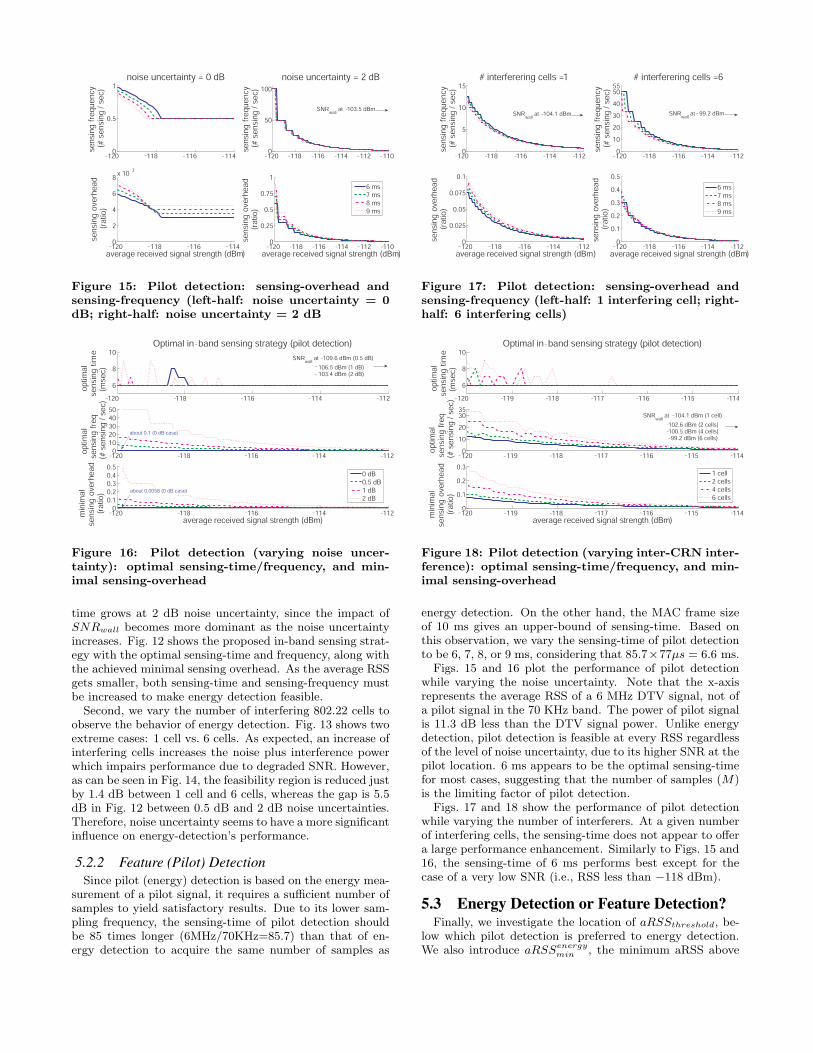
Figs. 15 and 16 plot the performance of pilot detectionwhile varying the noise uncertainty. Note that the x-axisrepresents the average RSS of a 6 MHz DTV signal, not ofa pilot signal in the 70 KHz band. The power of pilot signalis 11.3 dB less than the DTV signal power. Unlike energydetection, pilot detection is feasible at every RSS regardlessof the level of noise uncertainty, due to its higher SNR at thepilot location. 6 ms appears to be the optimal sensing-timefor most cases, suggesting that the number of samples (M)is the limiting factor of pilot detection.

Figs. 17 and 18 show the performance of pilot detectionwhile varying the number of interferers. At a given numberof interfering cells, the sensing-time does not appear to offera large performance enhancement. Similarly to Figs. 15 and16, the sensing-time of 6 ms performs best except for thecase of a very low SNR (i.e., RSS less than −118 dBm).

5.3 Energy Detection or Feature Detection?Finally, we investigate the location of aRSSthreshold, be-

low which pilot detection is preferred to energy detection.We also introduce aRSSenergy

min , the minimum aRSS above

120 115 110 105 1000

2

4

6

8x 10

3 noise uncertainty = 0 dBm

inim

al

se

nsi

ng

ove

rhe

ad

(ra

tio)

120 115 110 105 1000

0.02

0.04

0.06

0.08noise uncertainty = 0.5 dB

120 115 110 105 1000

0.025

0.05

0.075

0.1noise uncertainty = 1 dB

min

ima

l

sen

sin

g o

verh

ea

d(r

atio

)

average received signal strength (dBm) 120 115 110 105 100

0

0.025

0.05

0.075

0.1noise uncertainty = 2 dB


EnergyPilot

EnergyPilot

EnergyPilot

EnergyPilot

Figure 19: Energy detection vs. pilot detection: lo-cation of aRSSthreshold (while varying the noise un-certainty)

noise uncertainty 0.5 dB 1 dB 2 dBaRSSthreshold (dBm) −114.6 −112.5 −109.9aRSSenergy

min (dBm) −117.2 −114.6 −111.7

Table 2: aRSSthreshold and aRSSenergymin with various

noise uncertainty levels

which energy detection becomes feasible for detection ofDTV signals.

Fig. 19 compares the minimal sensing-overheads of energyand pilot detection under various noise uncertainty condi-tions. When there is no noise uncertainty, energy detec-tion is the best to use. As the noise uncertainty grows,however, pilot detection becomes preferable at a low aRSSand aRSSthreshold increases accordingly. The position ofaRSSthreshold is shown in Table 2 along with aRSSenergy

min .With 1 or 2 dB noise uncertainty, pilot detection is found tobe feasible and preferable even at −120 dBm, but it incursmore than 10% of sensing overhead.

aRSSthreshold and aRSSenergymin of various inter-CRN in-

terference are also presented in Fig. 20 and Table 3. With 1or 2 dB noise uncertainty, pilot detection is found to incurmore than 15% of sensing overhead at −120 dBm.

5.4 Other Feature DetectorsFrom Figs. 19 and 20, one can observe that energy detec-

tion, above aRSSthreshold, incurs at most 0.385% of sensingoverhead. Here, we compare this overhead with three othertypes of feature detectors than pilot-energy detection: thepilot-location detection in [43], the PN511 detection in [6],and the cyclostationary detection in [22]. Since sensing-times for such feature detectors are 30 ms, 24.1 ms, and19.03 ms, respectively, their sensing overheads are given asat least 1.5, 1.2, and 0.95 % even when sensing is sched-uled only once every CDT seconds. Therefore, energy de-tection performs better in its preferred region (i.e., aboveaRSSthreshold) than the pilot-energy as well as other threetypes of feature detectors under consideration.

6. CONCLUSIONIn this paper, we proposed an optimal in-band sensing

scheduling algorithm which optimizes the sensing-time andsensing-frequency of energy and feature detection, while meet-ing the sensing requirements in IEEE 802.22. Its perfor-

120 115 110 1050

0.02

0.04

0.06

0.08# interferering cells = 1

min

ima

l

sen

sin

g o

verh

ea

d(r

atio

)

120 115 110 1050

0.025

0.05

0.075


120 115 110 1050

0.05

0.1


min

ima

l

sen

sin

g o

verh

ea

d(r

atio

)

average received signal strength (dBm) 120 115 110 105

0

0.1



EnergyPilot

EnergyPilot

EnergyPilot

EnergyPilot

Figure 20: Energy detection vs. pilot detection: lo-cation of aRSSthreshold (while varying the inter-CRNinterference)

# of interferers 1 2 4 6aRSSthreshold (dBm) −112.9 −112.3 −111.3 −110.5aRSSenergy

min (dBm) −115.4 −115.1 −114.5 −114

Table 3: aRSSthreshold and aRSSenergymin with various

inter-CRN interference levels

mance has been evaluated extensively with respect to twoimportant factors: noise uncertainty and inter-CRN inter-ference. It is shown that energy detection under the shadow-fading channel is still feasible and effective in meeting the de-tectability requirements via collaborative sensing, and some-times preferred to feature detection even when the aver-age RSS is much lower than the power wall determined bySNRwall. The necessity of sensor clustering in CRNs is alsoelaborated, and two important problems, sensor cluster sizeand sensor density, have been addressed.

In future, we would like to explore other types of fea-ture detection and evaluate their performance comparativelywith energy detection. In-band sensing of wireless micro-phones should be another important subject of our futurework.

AcknowledgmentsThe work reported in this paper was supported in part by theUS National Science Foundation under grants CNS-0519498and CNS-0721529 and by industry grants from Intel Cor-poration, Philips Research North America, and NEC LabsNorth America.

7. REFERENCES[1] R. Tandra and A. Sahai. Fundamental limits on

detection in low SNR under noise uncertainty. In Proc.of the WirelessCom 2005, pages 464–469, June 2005.

[2] FCC. Spectrum policy task force report. ET DocketNo. 02-135, November 2002.

[3] FCC. Facilitating opportunities for flexible, efficient,and reliable spectrum use employing cognitive radiotechnologies. ET Docket No. 03-108, December 2003.

[4] FCC. Notice of proposed rule making and order. ETDocket No. 03-322, December 2003.

[5] S. Haykin. Cognitive radio: brain-empowered wirelesscommunications. IEEE J-SAC, 23(2):201–220,

February 2005.

[6] C. Cordeiro, K. Challapali, and M. Ghosh. CognitivePHY and MAC layers for dynamic spectrum accessand sharing of TV bands. ACM TAPAS, Aug. 2006.

[7] IEEE 802.22 working group on wireless regional areanetworks. http://www.ieee802.org/22/.

[8] G. Ganesan and Y. Li. Cooperative spectrum sensingin cognitive radio networks. In Proc. of the IEEEDySPAN 2005, pages 137–143, November 2005.

[9] E. Visotsky, S. Kuffner, and R. Peterson. Oncollaborative detection of TV transmissions in supportof dynamic spectrum sharing. In Proc. of the IEEEDySPAN 2005, pages 338–344, November 2005.

[10] A. Ghasemi and E.S. Sousa. Opportunistic spectrumaccess in fading channels through collaborativesensing. Journal of Communications (JCM),2(2):71–82, March 2007.

[11] A. Ghasemi and E. S. Sousa. Collaborative spectrumsensing for opportunistic access in fadingenvironments. In Proc. of the IEEE DySPAN 2005,pages 131–136, November 2005.

[12] A. Goldsmith. Wireless Communications. CambridgeUniversity Press, Cambridge, NY, 2005.

[13] T. Chen, H. Zhang, G.M. Maggio, and I. Chlamtac.CogMesh: A cluster-based cognitive radio network. InProc. of IEEE DySPAN, pages 168–178, Apr. 2007.

[14] C. Sun, W. Zhang, and K.B. Letaief. Cluster-basedcooperative spectrum sensing in cognitive radiosystems. IEEE ICC, pages 2511–2515, June 2007.

[15] P. Pawelczak, C. Guo, R.V. Prasad, and R. Hekmat.Cluster-based spectrum sensing architecture foropportunistic spectrum access networks.IRCTR-S-004-07 Report, February 2007.

[16] S. M. Mishra, A. Sahai, and R. W. Brodersen.Cooperative sensing among cognitive radios. In Proc.of the IEEE ICC 2006, pages 1658–1663, June 2006.

[17] M. Gudmundson. Correlation model for shadow fadingin mobile radio systems. Electronic Letters,27(23):2145–2146, November 1991.

[18] R. Tandra and A. Sahai. SNR walls for featuredetectors. In Proc. of the IEEE DySPAN 2007, pages559–570, April 2007.

[19] S. Shellhammer, S. Shankar N., R. Tandra, andJ. Tomcik. Performance of power detector sensors ofDTV signals in IEEE 802.22 WRANs. In Proc. of theACM TAPAS 2006, August 2006.

[20] S. Shellhammer and R. Tandra. Performance of thepower detector with noise uncertainty. IEEE802.22-06/0134r0, July 2006.

[21] S. Shellhammer and R. Tandra. An evaluation of DTVpilot power detection. IEEE 802.22-06/0188r0, July2006.

[22] H.-S. Chen, W. Gao, and D.G. Daut. Spectrumsensing using cyclostationary properties andapplication to IEEE 802.22 WRAN. In Proc. of IEEEGLOBECOM, pages 3133–3138, November 2007.

[23] L.P. Goh, Z. Lei, and F. Chin. DVB detector forcognitive radio. In Proc. of the IEEE ICC 2007, pages6460–6465, June 2007.

[24] D. Datla, R. Rajbanshi, A.M. Wyglinski, and G.J.Minden. Parametric adaptive spectrum sensing

framework for dynamic spectrum access networks. InProc. of IEEE DySPAN, pages 482–485, Apr. 2007.

[25] A.T. Hoang and Y.-C. Liang. Adaptive scheduling ofspectrum sensing periods in cognitive radio networks.In Proc. of the IEEE GLOBECOM 2007, pages3128–3132, November 2007.

[26] H. Kim and K. G. Shin. Efficient discovery ofspectrum opportunities with MAC-layer sensing incognitive radio networks. IEEE Transactions onMobile Computing (T-MC), 7(5):533–545, May 2008.

[27] A. Motamedi and A. Bahai. MAC protocol design forspectrum-agile wireless networks: Stochastic controlapproach. In Proc. of the IEEE DySPAN 2007, pages448–451, April 2007.

[28] S. Geirhofer, L. Tong, and B. M. Sadler. Dynamicspectrum access in the time domain: Modeling andexploiting white space. IEEE CommunicationsMagazine, 45(5):66–72, May 2007.

[29] S. Shellhammer. An ATSC detector using peakcombining. IEEE 802.22-06/0243r0, November 2006.

[30] M. Muterspaugh, H. Liu, and W. Gao. Thomsonproposal outline for WRAN. IEEE 802.22-05/0096r1,November 2005.

[31] N. Han, S. Shon, J.H. Chung, and J.M. Kim. Spectralcorrelation based signal detection method for spectrumsensing in IEEE 802.22 WRAN systems. In Proc. ofthe ICACT 2006, pages 1765–1770, February 2006.

[32] A. Sahai and D. Cabric. Cyclostationary featuredetection. Tutorial presented at the IEEE DySPAN2005 (Part II), November 2005.http://www.eecs.berkeley.edu/ sahai/Presentations/Dy-SPAN05 part2.ppt.

[33] V. Tawil. DTV signal captures. IEEE802.22-06/0038r0, March 2006.

[34] S. Shellhammer, V. Tawil, G. Chouinard,M. Muterspaugh, and M. Ghosh. Spectrum sensingsimulation model. IEEE 802.22-06/0028r10,September 2006.

[35] A. Sahai, R. Tandra, S.M. Mishra, and N. Hoven.Fundamental design tradeoffs in cognitive radiosystems. In the ACM TAPAS 2006, August 2006.

[36] M. Hata. Empirical formula for propagation loss inland mobile radio services. IEEE Transactions onVehicular Technology, VT-29(3):317–325, August 1980.

[37] E. Sofer. WRAN channel modeling. IEEE802.22-05/0055r0, July 2005.

[38] D. Mazzarese and B. Ji. Updated MIMO proposal forIEEE 802.22 WRAN systems. IEEE802.22-06/0015r0, January 2006.

[39] T.S. Rappaport. Wireless Communications: Principlesand Practices. Prentice Hall PTR, Upper SaddleRiver, NJ, 2nd edition, 2002.

[40] G. Chouinard. WRAN reference model. IEEE802.22-04/0002r12, September 2005.

[41] S. Shellhammer. Numerical spectrum sensingrequirements. IEEE 802.22-06/0088r0, June 2006.

[42] W. Caldwell. Draft recommended practice. IEEE802.22-06/0242r04, March 2007.

[43] C. Cordeiro, M. Ghosh, D. Cavalcanti, andK. Challapali. Spectrum sensing for dynamic spectrumaccess of TV bands. In Proc. of CrownCom, July 2007.

in-band spectrum sensing in cognitive radio networks ... · in-band spectrum sensing in cognitive...

Documents