Research Collection

Doctoral Thesis

The negative skin friction of bearing piles

Author(s): Elmasry, Mohamed Aly

Publication Date: 1963

Permanent Link: https://doi.org/10.3929/ethz-a-000088732

Rights / License: In Copyright - Non-Commercial Use Permitted

This page was generated automatically upon download from the ETH Zurich Research Collection. For moreinformation please consult the Terms of use.

ETH Library

Prom. No. 3262

The Negative Skin Friction

of Bearing Piles

THESIS

PRESENTED TO

THE SWISS FEDERAL INSTITUTE OF TECHNOLOGY, ZURICH

FOR THE DEGREE OF

DOCTOR OF TECHNICAL SCIENCES

BY

Mohamed Aly Elmasry

B. Sc. Civil Eng.

Citizen of the IT. A.R.

Accepted on the Recommendation of

Prof. G. Schnitter and Dipl. Ing. Ch. Schaerer

Zurich 1963

Dissertationsdrackerei Leemann AG

Leer - Vide - Empty

Contents

Synopsis 5

Preface 6

List of Symbols 7

Chapter 1: Introduction 11

1.0. Historical survey 11

1.1. Skin friction of piles 13

1.2. Present conceptions of the problem 14

1.3. Aim and scope of thesis 19

Chapter 2: Apparatus and adjustments 19

2.0. Main apparatus 19

2.1. Pile-construction and strain-gage measuring positions 22

2.2. Drag force measuring system 24

a) Apparatus used 24

b) Principle of bonded metallic strain-gages 25

c) Application of the principle to the problem measurements 27

1. Half-bridge circuit 27

2. External bridge-circuit 29

Chapter 3: Programme and experimental procedure 32

3.0. Discussion of the testing programme 32

3.1. a) Material used and its properties 34

b) Effect of colloid on the volume-weight of soil 34

3.2. Experimental advance 42

Chapter 4: Results of tests 45

4.0. Model experiment 45

4.1. Readings and results of the model experiment 45

4.2. Results of remaining tests 48

3

Chapter 5: Discussion of parameters and treatment of the problem by the ^-Theory . . 70

5.0. Discussion of relations between drag forces Fn and the different parameters 70

5.1. Relation curves between i^n and each parameter 72

5.2. Boundary conditions of the negative skin friction forces 74

5.3. Treatment by the 7r-Theory 75

Chapter 6: End formulae describing Fn 81

Chapter 7: Soil properties in relation to negative forces produced 86

7.0. Effect of pile movement and consolidation on the soil properties 86

7.1. Soil heave due to pile penetration 88

7.2. Mechanism of soil heave due to pile penetration 90

7.3. Discussion of the end soil properties produced 93

Chapter 8: Application 101

8.0. Calculation of a practical problem 101

8.1. Comparison of the various solutions 109

8.2. Measurements to be carried out in the field in order to comply with the

application of the attained formula 109

Chapter 9: Summary and Zusammenfassung 110

Bibliography 114

4

Synopsis

Settlement of a soil layer in which a pile is driven to bear on a firm stratum

tends to transfer load to the pile by negative friction. That is to say, the func¬

tion of the pile is to support not only its load from the superstructure but also

this drag force. The settlement may result from loading the soil on its surface,

for example by a fill or an embankement, and/or may be caused by the soil's

own weight if it is not yet consolidated.

This work analyses the mechanism of the phenomena known as negativeskin friction of -piles, on the one hand from the various points of views of

previous authors interested in this point and on the other hand by means of

a mechanical apparatus and electrical adjustments designed to permit the

solution of the problem following a special experimental analysis, in order to

overcome the assumptions which would have to be considered if a theoretical

treatment were followed.

A typical kind of soil producing the phenomena is used. The results of the

experiments are treated by dimensional analysis and the "77-Theory". The

soil properties attained in relation to the drag forces are also discussed.

The calculations lead to the determination of the value of the drag force Fn.A practical problem is solved by three different methods and a comparison is

given.

5

Preface

The present treatise gives a description of a practical method and a way to

contribute the drag forces which hang on pile foundations due to the settle¬

ment of adjacent soil. Tests were carried out in the Laboratory of HydraulicResearch and Soil-Mechanics at the Federal Institute of Technology in Zurich.

The series of experimental tests were carried out in 1959 and 1960 and were

proceeded by a preparatory test programme to decide if a solution of the

problem was possible.In January 1960 and during the experimental programme of this thesis

a theoretical treatment of the problem was completed and published by Messrs.

M. Buisson, J. Ahu and P. Habib of the Institut Technique du Batiment et

des Travaux Publics, Paris, under the title «Le Frottement Negatif». This

publication was received with interest, as the idea of trying to solve such a

problem which is of topical practical importance in a quantitative manner,

was conceived in the two institutes at the same time; this gave a good oppor¬

tunity of comparing the various methods, as will be seen in Chapter 8 of

this work.

As mentioned above, the investigations were carried out in the Laboratoryof Hydraulic Research and Soil-Mechanics at the Federal Institute of Techno¬

logy in Zurich. I am indebted to the Director, Professor G. Schnitter, and to

the Head of the Soil-Mechanics Laboratory, Dipl. Eng. Ch. Schaerer, for per¬

mission to carry out the tests and for valuable support during the work.

The staff of the laboratory also rendered assistance during the work. Mr.

G. Amberg, Mechanical Engineer, helped during the construction of the appa¬

ratus and with the development and performance of the strain-gage measure¬

ments and electronic apparatus. Mr. E. Briigger contributed the photographs.Mr. B. Zwahlen, mathemathician at the ETH, revised the mathematical

treatment due to the dimensional analysis and the 7r-Theory.I express my gratitude to the above-mentioned colleagues and to the

laboratory personel.The printing of the treatise has been made possible by the financial support

of the Egyptian Government.

6

List of symbols

In the following pages, we desire to state expressely that by drag-force, or

force of negative skin friction, is meant the total force which hangs on to the

pile due to the settlement of the adjacent soil. It is denoted "Fn". The partwhich results from the consolidation of the surrounding soil under its own

weight only is denoted by "Fn_s".The following list contains the most important symbols that will appear.

Wherever other notations are used only by mentioned authors, their notations

are written at the corresponding places.

General

77 = 3.1416.

e = the base of natural logarithms = 2.7183.

t = time.

g = the gravitational acceleration.

Stress and strain

a = normal stress.

a = normal effective stress.

t = shear stress.

8 = displacement.e = specific normal strain.

u = pore-water pressure.

ME = modulus of compressibility of soil.

Soil properties

a) Density, porosity, etc.

ys = density of solid particles.

y* = wet volume-weight, bulk density. (ye* initial and y* final.)

yd = dry volume-weight.

7

y'e = saturated volume-weight.

y"e = submerged volume-weight.

yfia= volume-weight of the fill, embankment, surcharge, etc.

yK = appropriate volume-weight of the corresponding soil layer.

yw = density of water.

W % — percentage water-content. (Wa % initial and We % end.)

e = void ratio.

n = porosity.S = degree of saturation.

b) Consistency, etc.

for cohesive soils:

LL = liquid limit.

PL = plastic limit.

Pj = plasticity index = LL — PL.

Lj = liquidity index =

—p—-.

Cj = consistency index = ~^=—.

Activity is defined by Skempton as the ratio of P2 to content of clay finer

than 2 microns.

for non-cohesive soils:

emax = void ratio in loosest state.

emin — v°id ratio in densest state.

RD — relative density = —r^_——.

c) Shear strength

ri and Tf= initial and final shear resistance respectively.

rp_s= frictional resistance between the pile and the soil.

G = apparent cohesion.

0 = angle of shearing resistance, in terms of total stress in the equation:t = C + a tan<£.

0' = real angle of shearing in the equation: t = C' + or' tan <£>'.

C" = cohesion.

d) Permeability

h = hydraulic head.

^ a i iV water volume

Q = flow/second =

T=

^ .

8

v = velocity of flow.

i = hydraulic gradient.J = seepage gradient.k = Darcy's coefficient of permeability.

e) Consolidation

p = pressure (overburden, consolidation, etc.).

pc = consolidation pressure.

acc = coefficient of compressibility = —

-r—.

mcc = coefficient of volume decrease or specific compressibility:

arr -de,yyt

^

'M

(l + e0) dp(l+eoy

— onrkTTimriY\'t' nT nr\Y\vr\\ir\(~\'i"irtY\ —cre

— degree of consolidation.

Tm = time factor = —=- ==r.

a2 mVc yw a2

Pile symbols

G = the pile's own weight.P = load acting on the pile due to the superstructure P1,P2,PZ... etc.

U = pile perimeter.

/ = pile cross-sectional area.

8 = height of the pile-shoe or pile beckel.

n' = number of piles /unit area.

n" = number of piles /cluster of piles.F = horizontal area served by the pile.H = thickness of soil layer.Z — co-ordinate of depth.h = pile penetration.0 = neutral point on the pile axis.

Strain-gages

A = active strain-gage.K = temperature compensation strain-gage.R = resistance of gage wire.

9

dEn = increment of wire resistance due to normal stress.

dEb = increment of wire resistance due to buckling stress.

dRg = increment of wire resistance due to temperature variation stress.

0 = oscillator.

U0 = oscillator potential drop.

Um = meter potential drop.UB = battery potential drop.m = Poisson's ratio.

k = strain-gage factor.

10

CHAPTER 1

Introduction

1.0. Historical survey

For more than thirty years the action of negative skin friction in pile foun¬

dations has been known in a qualitative manner. In some cases the damagein the project could have been counteracted, and in other cases completecollapse took place. The following are some of the actual examples which were

encountered.

a) The Jurgens Margarine Company erected an oil mill containing heavyequipment at Zwyndrech in Holland. The site was land made of hydraulic fill.

The soil consists of about 5 m of sandfill, about 15 m of peat and clay, 6 m of

fine sand, then the coarse sand and gravel at the bottom. All soils were satu¬

rated. Test piles were driven to a resistance of 50 tons per pile.Creosoted wood piles 22 m long were used. Pile points stopped in the fine

sand about 3 m above the coarse sand and gravel. In four years the buildingsettled 70 cm near the centre, threatening collapse. Maximum settlement did

not occur under the heaviest loaded piles, which carried 18 tons each. Piles

under an outside extension with almost no load settled similarly.The cause of failure was the negative friction owing to the settlement of

the hydraulic fill which added an estimated load of 15 tons per pile, and over¬

loaded the pile points in the fine sand.

The remedy consisted in underpinning to firm material under the fine

sand [25]1).

b) Wood piles for a water structure were driven through rocky fill into

firmer soils. Driving resistances were considered ample according to dynamicformulas, but the force imposed on the piles by subsidence of the fill and com¬

pression of soft bay deposits was so great that a pile was pulled down from

the concrete foundation of the structure it was intended to support, so that

the head of the pile was several inches below the concrete caps.

A later boring showed 13 m of sandy loam and rock fragement fill, 9 m of

J) Numbers between brackets refer to the bibliography at the end of this work.

11

soft bay mud, 6 m of firm clayey soil, then decomposed rock against which

the tip rested. The potential downward load of the gripping fill was estimated

to be 175 tons, and that of the bay mud to be 12 tons. Some portion of these

loads probably fractured the pile, permitting the upper part to slide by the

lower part resting on the rock.

The cause of failure was the additional load from fill and compressiblestratum, and reliance upon driving formula.

No remedy is stated [7].

c) A serious case arose from the placing of a heavy fill surrounding a con¬

crete stadium which was provided with sufficient concrete piles to carry safelythe loads from the structure, but where the piles were unable to carry the

added load due to the settlement of the soil compressed by the much greaterload from a fill placed outside of and around the structure.

The cause of failure was the addition of load from fill above compressiblestrata.

No remedy was stated [26].

d) This case of failure represents one of the disatrous results of inadequateknowledge of soil conditions and reliance on results of load tests made on a

single pile.The chimney of a textile factory is located on the left side of Mahmudia

Canal in Alexandria, Egypt, in an area reserved for industrial factories. Before

deciding on the type of foundation for the factory and chimney, borings were

made in the area. The top 2 m were filling material followed by 2.6 m of weak

grey clay mixed with sea shells, 5.5 m of very weak dark clay mixed in the

last 1.0 m of its thickness with shells, 3.5 m of stiff yellow cohesive clay, 1.0 m

of sand on a sand stone bed extending for big depths. The contractor decided

to erect the factory and chimney on floating pile foundations. The piles used

were cast-in-place piles of length 5 m, bringing the toe of the pile just to the

top of the dark clay layer, which has a thickness of 5.5 m.

A load test on a single pile was indeed carried out, and the result of the

test gave a load of 70 tons.

The measurement of settlement began when the load on the pile was 20 tons,which is the load of the reinforced concrete cap. From the load test the con¬

tractor decided that 35 tons would be a safe load per pile.The weight of the chimney was 1100 tons. The settlement observations

began as soon as the chimney was 1.0 m high above the ground level. On

completion of the chimney, the settlement at one side was 12 cm, and at the

opposite side 17 cm, a value ranging from 40 to 57 times the settlement of the

test pile under the same load per pile. After the completion of the chimney the

settlement continued until it amounted to 27.6 cm on one side and 43.6 cm

on the other.

12

The cause of failure was that the pile could not carry the additional loads

which came from the settling soil.

As a remedy it was tried to reduce the stresses on the soil by extending the

base, but without success — and the complete structure was demolished [13].e) Batter piles were driven to resist the outward movement of a quay wall

constructed in 10 m of silt-laden water. Sheet piles for retaining the fill below

and to the rear of the relieving platform were driven 13 m back of the face

of the wall, thus exposing the batter piles under the relieving platform to the

accumulation of silt deposit. Frequent dredging left banks of soft mud under

the wall held against rapid sloughing down into the stream by the piles. This

added load from skin friction on the batter piles produced settlement of the

piles, and instead of resisting the outward movement of the wall they pulledit forward, so that the wall moved outward several feet.

The cause of failure was the drag from mud sloughing caused by dredging.No remedy is stated [26].

f) At a site of a proposed abutment for a bridge on the Connecticut Turn¬

pike a fill approximately 16 m high was placed on top of a layer of marine

mud. It was anticipated that consolidation of the soft mud layer would not

be complete at the time the supporting piles for the abutment were driven

to a firmer stratum underlying the mud. Therefore a particularly severe load¬

ing condition for drag forces might be imposed on the piles.In view of the uncertainties involved in the design of the pile foundation

for drag forces, an experimental investigation of the nature and magnitudeof these forces was made.

The result was that drag forces of large magnitude were found to hangover the piles [14].

Further cases are described by Terzaghi [2], Chellis [1], Moore [7], Florentin

and L'Heriteau [6] and others interested in this problem.

1.1. Skin friction of piles

It is known that the direction of the skin friction of piles is that of the

movement of the adjacent soil mass with respect to the pile. If the pile moves

downward under the action of the load, this means that the relative motion

of the mass of earth is upwards and the skin friction develops upwards also.

This happens, for instance, in incompressible soil.

If the earth mass consolidates, the direction of the skin friction is downward

(so called negative friction). Thus the point of the pile has also to carry a partof the weight of the soil and/or the surcharge around the pile; this weight is,

13

so to speak, hanging on the pile [4]. As a rule negative friction is a dangerousfactor, since it increases the acting load and causes an unexpected settlement

of the structure.

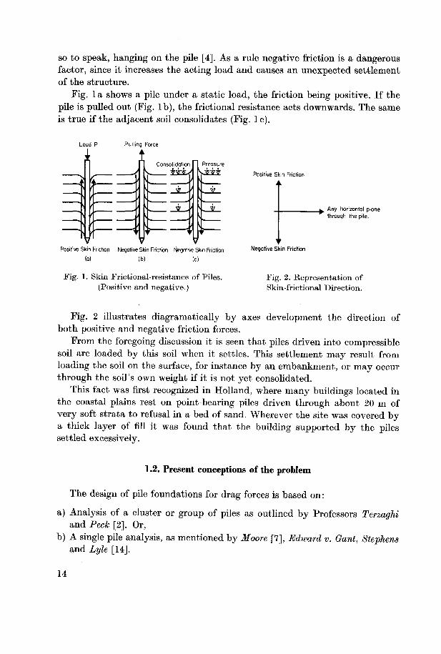
Fig. 1 a shows a pile under a static load, the friction being positive. If the

pile is pulled out (Fig. lb), the frictional resistance acts downwards. The same

is true if the adjacent soil consolidates (Fig. lc).

Positive Skin Friction

^ Any horizontal plane

through the pile

Skin Friction

Fig. 1. Skin Frictional-resistance of Piles. Fig. 2. Representation of

(Positive and negative.) Skin-frictional Direction.

Fig. 2 illustrates diagramatically by axes development the direction of

both positive and negative friction forces.

From the foregoing discussion it is seen that piles driven into compressiblesoil are loaded by this soil when it settles. This settlement may result from

loading the soil on the surface, for instance by an embankment, or may occur

through the soil's own weight if it is not yet consolidated.

This fact was first recognized in Holland, where many buildings located in

the coastal plains rest on point-bearing piles driven through about 20 m of

very soft strata to refusal in a bed of sand. Wherever the site was covered bya thick layer of fill it was found that the building supported by the pilessettled excessively.

1.2. Present conceptions of the problem

The design of pile foundations for drag forces is based on:

a) Analysis of a cluster or group of piles as outlined by Professors Terzaghiand Peck [2]. Or,

b) A single pile analysis, as mentioned by Moore [7], Edward v. Gant, Stephensand Lyle [14].

Load P Pulling Force

Positive Skin Friction Negative Skin Friction Negative Skin Friction

(a) (b) (c)

14

1.2.1. Estimation of drag forces by Terzaghi and Peck

Hypothesis

Before the piles are driven, the compressible strata consolidates graduallyunder its own weight and/or the weight of the newly applied fill, and the fill

settles as soon as the piles are installed. The fill material located in the upper

part of the pile cluster can no longer settle freely because its downward move¬

ment is resisted by the skin friction between the fill and the piles. The down¬

ward motion of the fill with respect to the piles transfers the weight of the

fill located within the cluster on to the piles.

Symbols. If:

A = the area of the horizontal section included within the boundaries of

the cluster.

n" = the number of piles.H = the thickness of the fill.

ym— the unit weight of the fill.

Q' = the load which acts on each pile due to the weight of the fill within the

cluster.

Then: Q' = £-ymH. 1.2.1(1)

In the space between clusters, the weight causes progressive settlement. If

the cluster consists of point-bearing piles, the piles do not participate in the

downward movement. In consequence the soil surrounding the cluster moves

down with reference to the cluster and tends to drag each cluster down. The

drag increases as the consolidation of the soil surrounding the cluster proceeds.This force cannot be more than:

Q'Lx=~Hr. 1.2.1(2)

which is the top limit.

Where:

Qmax = the maximum load acting on the pile due to the soil weight.L = the circumference of the cluster.

n" = the number of piles.H = the thickness of the soil stratum.

t = the average shearing resistance of the soil.

The actual value Q" ranges between zero and Q"max. We had no means of

determining it except by an estimation based on judgement.

15

The drag force or negative skin friction force:

Fn = Q' + Q".

If Q is the load per pile exerted by a building, the lower end of the pilewill ultimately receive a total load of:

Qt = Q + Q' + Q"- i.2.i(3)

If Qt is greater than the point bearing resistance of the pile, the settlement

of the foundation will be excessive, regardless of what ultimate capacity a

load test may indicate.

Therefore Qt and the point resistance of the pile must be known.

1.2.2. Contribution of drag forces by M. Buisson, J. Ahu and P. Habib [15]:Theoretical treatment

Hypothesis

Although the existence of negative skin friction forces seems to be a simple

phenomenon, its experimental treatment is extremely difficult. The following

assumptions are made in order to permit a theoretical solution:

1. The bearing soil in which the pile penetrates is homogeneous and limited

by a horizontal plane.2. The compressible soil taken into consideration overlays the bearing soil. Its

natural properties are homogeneous and constant up to the top surface,

which is assumed to be horizontal. The soil is pure cohesive and <& = 0. It

is also assumed that no consolidation has previously taken place.3. The pile under consideration is dynamically forced into the soil, and sur¬

rounded by other piles driven in the same way. The distance between the

piles is considered to be a maximum of 1/3 to 1/i of the thickness of the

compressible layer.4. The soil is assumed to have the same homogeneous compressibility in the

horizontal section.

5. The soil is assumed to be charged directly after the driving of the piles,and with an intensity which is uniform and endless.

6. Each of the piles and the soil is treated separately and the two equationsare solved together.

7. The surcharge exerts on the pile a stress of a value:

Where:

r = the total force exerted on the pile by the fill.

F = the area concerning the pile.

16

®sina= a constant = 0.30.

ym = the volume weight of the fill.

hfiU = the height of the fill.

U = the perimeter of the pile.

8. The pressure curve of the soil at the initial instant is considered to be a

uniform parabola.

Notation:

P = the load acting on the pile due to the building./ = the cross-section of the pile.

yE = the volume weight of the compressible soil.

H = the thickness of the compressible strata. If we put y'E for H' and

y"E vor H", where: H = H' + H",

then: yEH = y'EH' + yEH".Z = the depth along which the negative friction acts.

ri = the initial shearing resistance of the soil.

Tf= the final shearing resistance of the soil.

Qz = the reaction of the working forces at the pile toe.

Equations of equilibrium

Equation (I)P + r + TfUZ-rfU(H-Z) = Qz,

from which: P + r + rfU(H-2Z) = Qz- (!)

The unknowns are: Z and Qz.

We therefore need a second equation.

Equation (2). The velocity of penetration of the pile and that of the com¬

pressibility of the soil are equal at a neutral point on the pile axis.

Let us consider an element of soil having a thickness dZ, which will be

compressed and show a settlement d y.

Therefore:

dy = dZAn, where An is the change per

unit volume of the soil

and A n = —-^y = ^-^ = mvcA p (see Fig. 3),

where: e = void ratio.

a„c = modulus of compressibility.

mcc = modulus of specific compressibility.

.-. y = fmvcApdZ. (2)z

17

Solution

Equations (1) and (2) are solved graphically to give Z and hence Qz.

Note. In Chapter 8, we shall revert to the detailed treatment of this method

in accordance with reference 15.

pm— Pc—«|

Fig. 3. Consolidation-pressure curves.

pc Pressure of the fill.

r and F as given in the assumptions.

O and O' are neutral-points on the pile axis.

ab c and a V o' represents the curve of influence due to the pile movement downwards,

and a b' begins from point a and increases by a value of t/• U/F per unit length

of the pile, till it reaches the horizontal plane passing through the neutral point O

or O' (O and O' are the neutral points of which the depth from the soil-surface

is to be calculated as shown in Chapter 8). It then decreases at the same rate

up to the point core' respectively.

is the curve representing the consolidation pressure due to the soil's own weight,

is the curve representing the consolidation pressure due to the soil's own weight

+ surcharge.

a b

(co)

(c)

18

1.3. Aim and scope of thesis

This treatise has as its subject the negative skin friction produced in bearingpile foundations, which is produced by the settlement of adjacent soils.

According to Terzaghi it is considered to be composed of a force acting down¬

wards of a value equal to the weight of the fill, plus another force which is a

function of the compressible soil thickness and the mean shearing resistance

of the soil, this being considered to have values ranging from zero to a maxi¬

mum value.

The relation between the drag forces and the various parameters is discussed,and an attempt is made to obtain expressions for the magnitudes of the dragforces.

A description of the apparatus and measuring methods used for experi¬mental determination of these forces is given and the experimental programmeis applied to a typical soil for producing drag forces.

A practical problem is solved by three different methods, namely that of

Terzaghi, the French method, and the application of the formulae obtained

by this experimental work. Finally a comparison is given.The present work cannot be considered a complete analysis of all questions

concerning the negative skin friction of piles. Rather it should be regarded as

a beginning, a description and an interpretation of an experimental analysisof this field of research.

CHAPTER 2

Apparatus and adjustments

2.0. Main apparatus

The main apparatus is designed and constructed to serve two principal

purposes:

a) A large-scale consolidation apparatus with a 10:1 cantilever arm, i.e.

giving a consolidation concentrated load of ten times the weight put on the

pan directly on the center of a piston shaft which is concentric with a material

container of cylindrical form. The load is uniformly distributed by a circular

plate having the same cross sectional area as the cylinder.The weight of the cantilever beam and accessories can be equalised by a

system of pulleys and counterweights (Fig. 4a and b). The compressibility is

measured by extensometers.

19

©

i m?

0,125

2 L 40x40x5

L25x25x3

—i h

62,0

40,0

B WC,120x60

3,20t D

4x5

1,80 m

1

1,65m

£t

S

Cylinder * = 32 cm

62 0 L = 62 cm

C 100x50

U

0,125

CONCRETE

6x8,5

BASE

I,75x0,40x0,40m

-JW*

0 01 02 03 04 05 m

DETAIL A

020 m

^ii—

r0

DETAIL B DETAIL C

Fig. 4a.

OI8m

042m

Fig. 4 b. Main apparatus showing the

counterweight system of the cantiliver

beam.

Two cylinders were designed for the apparatus, one having a cross-sectional

area of 800 cm2 (diameter = 32 cm) and serving the treatise work, and the

other, of cross-sectional area of 500 cm2 (diameter = 25 cm), being used for

consolidation purposes.

b) The following is the auxiliary equipment designed and constructed to

suit the experimental programme only:1. An upper circular rigid steel plate (diameter = 25 cm), screwed con¬

centrically from above to a vertical pole one meter high which serves to main¬

tain the pile load P centrally in position. The load P consists of the required

number of lead discs each weighing 10 kgs and having a central hole and side

slot to admit the vertical pole into the circular hole.

2. The circular steel plate is screwed centrally from below to a vertical

scale graduated so as to read the pile penetration from any position. This is

guided to move in a vertical path coinciding with the vertical axis of the

cylinder and that of the pile, this being done by means of a rigid guide fixed

to the frame of the structure (Fig. 5).

3. The lower end of item 2 can be screwed to a circular cover which fits

into the pile.4. The cylinder of area 800 cm2 is the soil container, having a diameter of

32 cm. It is thus six times the pile diameter, which is <&piie = 5 cm. The layer

thickness of the soil in the cylinder can be varied as required (see programme).

5. The toe of the pile rests on a sandy layer; the latter also acts as a down¬

ward filter, which is drained. At the upper surface of the soil a rigid perforated

plate serves as:

a) An upper filter plate.

b) To measure the soil compressibility with respect to time. This is done

21

by means of two extensometers adjusted by two fixed vertical poles at oppositeends of a diameter.

c) A base for carrying the consolidation loads pc, which can be increased

as required. These consist of circular lead plates, each of two halves beingfitted with half circular holes around the pile and the extensometer poles.

Fig. 5. Main apparatus with measuring

equipment during an experiment.

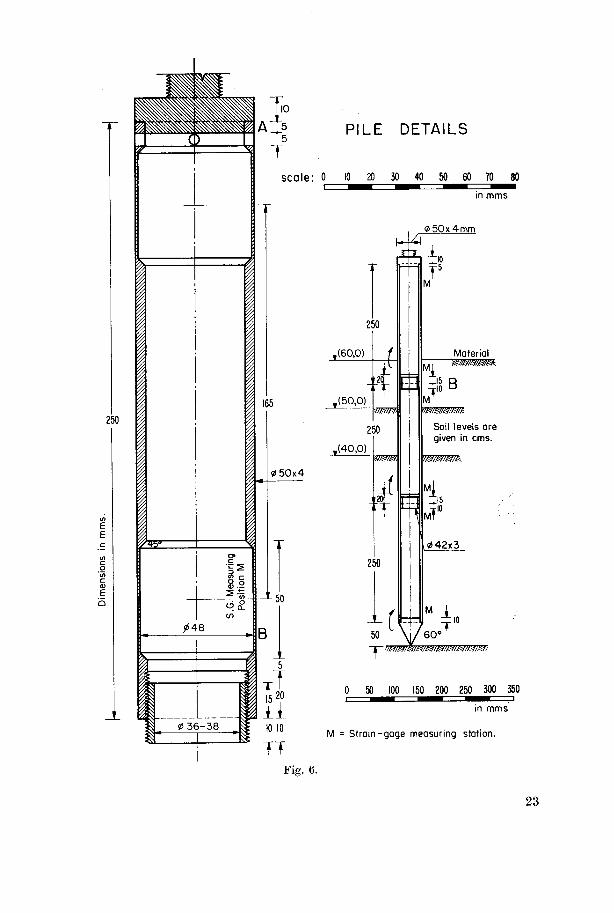
2.1. Pile construction and strain-gage measuring positions

a) Pile material

The pile is a steel pipe (steel 44), stainless plated, having a = 44 — 58 with

8 —4 % strain S10. The pile shoe is made of the same material and is solid,

height = 50 mm. with a screw-fitting at the circumference of its top surface

to be screwed to the pile, the slope angles are 60°.

b) Gage installation

One of the important points in the experimental work was the measuring

positions and gage installation. Several preliminary studies were made to

determine the most efficient method of gage installation and location of the

measuring positions. One method was to have two positions at the upper and

22

250

*48

0 36-38

PILE DETAILS

scale: 0 10 20 30 40 50 60 70

0 50x4

- -»-50

B

3

is 20

h-Kr

250

,(60,0)

,(50,0)

4

250

,(40,0)ssws

i 20

E3

0 50x4mm

«^io

Material

-15 R

M

Soil levels are

given in cms.

mmmt

4

mT

0 42x3

M _^

50 ~W60°

0 50 100 150 200 250 300 350i ^— — ^— 1

in mms

M = Strain-gage measuring station.

Fig. 6.

23

lower ends of the pile. Strain-gages were fitted inside. A trial was also carried

out with measuring positions in which strain-gages were fitted from the out¬

side surface of the pile in circular grooves, the whole groove being afterwards

covered with special cementit material after the installation of the gages; this

too proved to be unsatisfactory. A third method, which was also unsatis¬

factory, was the installation of gages through holes made in the pile at the

required positions.However, after many trials the method illustrated in Fig. 6 was adopted.

The procedure was as follows:

1. The pile was prepared in the Institute workshops as detailed in Fig. 6,

with the measuring positions containing the gage axes marked on them.

2. The cables used were of the type recommended in the specifications of

the strain-gages used.

3. Type SR-4 electric strain-gages were installed with the special duco

cement at the intervals shown. Two active gages were provided at each station

with another two temperature compensating gages in order to avoid the

buckling effect, if any, although the apparatus was designed to avoid buckling.4. The gages were then glued to the pile shell, waterproofed and given

mechanical protection. An asphalt paving cement was spread over the whole

station and fused to the steel by curing with heat lamps.5. All parts of the pile were screwed together and sealed with araldit at the

contact surfaces.

c) Check on measuring stations

Before sealing each station two checks were made:

1. Each strain-gage was checked separately with a resistance meter bridgeto make sure that it was not broken and its resistance complied with the

specification.2. A compression and release static load test was carried out on each station

to verify that all the strain-gages acted together.

d) Properties of strain-gages used

R = 120 Ohm + 0.25 %

k = 2.02 ± 1.0 %

2.2. Drag force measuring system

a) Apparatus used

Strain-measuring experiments were carried out with various types of strain-

indicating apparatus, to choose the most sensitive and satisfactory one for

24

the experimental requirements. Peekel electronic strain-indicating apparatus

Type B-103 U was used because it:

1. Has four measuring inlets at the same time.

2. Can be used for both half and external bridge circuits.

3. Can be easily checked before each set of measurements.

4. Indicates from 0—30 000 microstrain, (1 microstrain = 1-10~6 = fie.)5. Works on the manual null-method.

6. Enables the batteries to be changed easily when required. Fig. 5 shows the

apparatus during an experiment.

b) Principle of bonded metallic strain-gages

1. History and use in foundation and soil-mechanics measurements

The idea of bonding the resistance element directly to the material was

conceived at the California Institute of Technology in connection with a ten¬

sion impact test. This apphcation was made by Simons and reported by Clark

and Datwyler 1938 [20, 21]. In this case approximately 14 feet of No. 40

constantan wire was laid longitudinally on four successive faces of a bar in

zigzag fashion and coated with glyptal as a binder. The wire was protected

by Scotch tape. The complete unit was used as a dynamometer in impact

testing.

Ruge at M.I.T. at about the same time conceived the idea of bonding the

wire to paper and then bonding the paper with a common glue to the material

of which the strain is to be measured.

This bonded wire type of electrical-resistance strain-gage is cemented to

the surface of the structural member to be tested. Two constructions of gage

are shown in Fig. 7.

The strain-sensitive wire is about 0.025 mm diameter. These fine alloywires are soldered or welded to heavier copper wires. This type of gage is

typified by the SR-4 gage manufactured by Baldwin Southwark [19].

.Lead wires Gage wires Leod wires" Paper winding form

Paper base Paper base

(a) Flat grid type. (b) Helical coil type.

Fig. 7. Showing two types of strain-gage construction.

25

During the past ten years [6, 7, 22] the use of bonded strain gages has been

adopted for strain measurement in soil-mechanics and foundation engineering.

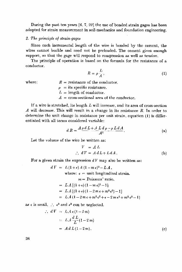
2. The principle of strain-gages

Since each incremental length of the wire is bonded by the cement, the

wires cannot buckle and need not be preloaded. The cement gives enoughsupport, so that the gage will respond to compression as well as tension.

The principle of operation is based on the formula for the resistance of a

conductor.

R=p^t> (i)

where: R = resistance of the conductor.

p = its specific resistance.

L = length of conductor.

A = cross-sectional area of the conductor.

If a wire is stretched, its length L will increase, and its area of cross-section

A will decrease. This will result in a change in its resistance R. In order to

determine the unit change in resistance per unit strain, equation (1) is differ¬

entiated with all terms considered variable:

, „ ApdL +ALdp-pLdAd R = — nr^—

Let the volume of the wire be written as:

V = AL

;. dV = AdL + LdA. (b)

For a given strain the expression dV may also be written as:

dV = L(l + e)A(l-me)2-LA,

where: e = unit longitudinal strain.

m= Poissons' ratio.

= L4[(l + «)(l-m6)8-l]

= LA[{l+e){l-2me+ m2e2)-l]

= LA(l — 2nie + m2e2 + e-2me2 + m2e.3 — l)

as e is small, .'. e2 and e3 can be neglected.

.-. dV = LAc{l-2m)

= LA~(l-2m)

= AdL(l-2m). (c)

26

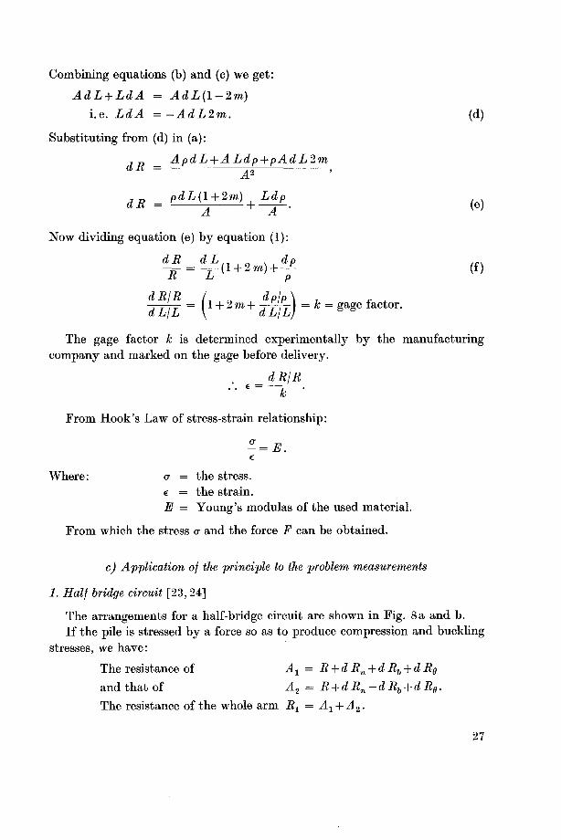
Combining equations (b) and (c) we get:

AdL + LdA = AdL(l-2m)

i.e. LdA =-AdL2m. (d)

Substituting from (d) in (a):

JD ApdL +ALdp+pAdL2mdR =

-g ,

dR =

PdL(l + 2m1+LdfL (e)

Now dividing equation (e) by equation (1):

dR dL^ dp ...

^R"=

^(1 + 2m)+ (f)

iw = (1+2m+imj=k=gage factor-

The gage factor k is determined experimentally by the manufacturing

company and marked on the gage before delivery.

_

dRjR••

e~

k"

From Hook's Law of stress-strain relationship:

Where: a = the stress,

e = the strain.

E = Young's modulas of the used material.

From which the stress cr and the force F can be obtained.

c) Application of the principle to the problem measurements

1. Half bridge circuit [23,24]

The arrangements for a half-bridge circuit are shown in Fig. 8 a and b.

If the pile is stressed by a force so as to produce compression and buckling

stresses, we have:

The resistance of Ax = R + d Rn + d Rb + d Rg

and that of A2 = R +dRn — dRb + dRg.

The resistance of the whole arm Rx = A1 + A2.

27

Active strain-gages

Compensating gages

o

o

I

oCV1

Amplifier

¥>1— Earth

o

I

o

G

oli

Fig. 8 a. Electronic strain-measuring apparatus adjusted on half-bridge circuit.

A\,A% — active gages to the pile axis.

Ki, K2 — temperature compensators perpendicular to pile axis.

U = IxR (in general).

Ri, R2, -B3 and Ri are the arm resistances.

Fig. 8 b. Details of bridge circuit and measuring position. Arrangements for a half-bridgecircuit.

28

29

2dRg)'+dRn-dRb+{2R

dRe)+U0(R

2dRg)'+dRb+dRn+(2R

dR0)+dRb+dRn+Uo(R

^3+^i/2

=u*

=Ux

and

Rj'+R^R2+\R1

\u.r,UpR,Ium=u1-u2

have:weway,sametheinProceeding

dRg.+R=i?4isK1ofresistanceThe

dRb.—dRg+dRn+R—RsisA2ofresistanceThe

dRg.+R~R2isK2ofresistanceThe

dRb+dRg.+dRn+R=RxisAxofresistanceThe

have:we9b,Fig.from

andcase,previoustheindiscussedasforcestressingsametheConsidering

circuit.external-bridgeanforarrangementstheshowsbanda9Fig.

24][23,circuitExternal-bridge2.

"

R4

dRnUpdRntt_

)]2~RTRRidRnd

R2R

2R

dRe+

R{dRndRgd

R

H2)R2R)\1dRg\dRnI\

R+

R+

+

-i1R„

(d

+i?^(i_RWd

,\2jB

i0 E2l1+

¥)+•(i+£!)^R+TT(•

Un=

C7„=

Un=

Um=Un

Rg),d+(i?+i?fl)rf+(i?=-ftT2+is^=i?2is2armofresistancethe

where:

2J'2dRe)+dRn1]

dRB)+dRn

+2(2R

dRe)+dRn

+2{R

i?4+R3

R3U0£/,and

R2+R±

and

Ra'+R»

Upjand

R.U,

R2-E^-f

un

U1

h

have:we8Fig.From

Arrangement for an external-bridge circuit.

Fig. 9 a. Strain-measuring apparatus adjusted on external-bridge circuit.

Ri = R + dRn + dRb + dRgR2 = R + dRff

Ri = R + dR„-dRb + dRgRi = R + dRa

Y~

K,or

IHHA, a2

Al.

Fig. 9 b. Details of bridge circuit and measuring position.

30

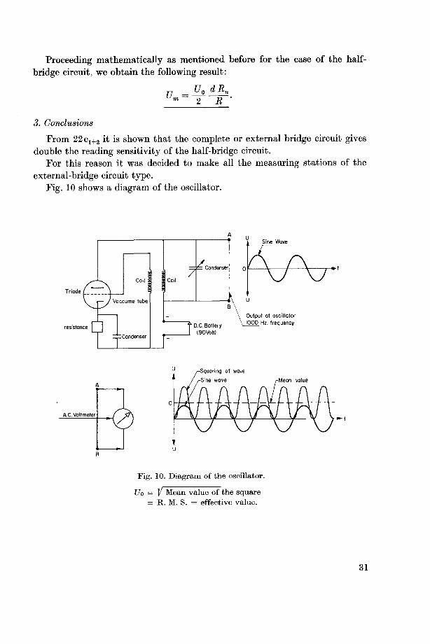
Proceeding mathematically as mentioned before for the case of the half-

bridge circuit, we obtain the following result:

Um =

R

3. Conclusions

From 22c1+2 it is shown that the complete or external bridge circuit givesdouble the reading sensitivity of the half-bridge circuit.

For this reason it was decided to make all the measuring stations of the

external-bridge circuit type.

Fig. 10 shows a diagram of the oscillator.

Output of oscillator

~t D C BatteryV l00° Hz frequency

(90Volt)

A C Voltmeter

Fig. 10. Diagram of the oscillator.

Uo = V Mean value of the square

= R. M. S. = effective value.

31

CHAPTER 3

Programme and experimental procedure

3.0. Discussion of the testing programme

a) Material used

As shown in Chapter 1, the soils which produce negative skin friction

phenomena are those which possess high compressibility and which are not

yet completely consolidated, namely either partially consolidated under its

own weight, or already consolidated under itself but able to consolidate further

due to a stress increment produced for instance, by a fill weight. On the other

hand, it was desirable to find a natural kind of soil material which complieswith the required properties. A number of trials were made with materials

from various locations in Switzerland. Standard laboratory tests were made to

compare them, and it was decided to carry on the experimental work with the

material lab. No. 11190 — a silty sand with clay, as will be described in

section 3.1.

b) Parameters

1. Consolidation pressure pc

A varing parameter having values of 0.1, 0.2 and 0.3 kg/cm2, i.e. 1, 2 and

3 t/m2 respectively.

2. Thickness of compressibile soil-layer H

Taken to be a variable parameter of values 60, 50 and 40 cm respectively.

3. Dry-volume weight of the soil yd

(or wet-volume weight y*)

A variable parameter of values 1.53, 1.63 and 1.66 g/cm3 or t/m3 respec¬

tively. (y*= 1.90, 2.00, 2.05 resp.) See 31b.

4. Initial water-content of soil Wa %

As the soil material in its natural condition has no plasticity, it did not

give any liquid limit. The water-content in the tests was therefore related to

the optimum moisture content according to Proctor experiments carried out

at the beginning, instead of consistency relations. Water-content Wa % varied

between 1.0 and 1.5 times the optimum, in which the optimum water content

is taken as 15 %. For the latter (1.5 opt.), the material was nearly saturated.

32

The above-mentioned parameters are those which are thought to be the

variables affecting the negative skin-friction. In addition, the specific gravityof the soil ys, which varies within a small range for the majority of materials

(from 2.65 to 2.85 t/m3), will affect the negative friction through the volume-

weight of the soil in the relation:

Furthermore, as the problem under consideration is a bearing pile problem,the pile load P was taken as constant throughout the experimental programme.

c) Tabulated experimental programme

The testing programme consisted mainly of four series of experiments,each consisting of three experiments in which one parameter varies and the

Table 1. Skeleton of test programme. (For § see 31b.)

Series

No.

Exp.No.

Variables Constants Degreeof satu¬

ration

s %

Pc H Wa Yd*

Ye0

kg/cm2 t/m2 cm /o g/cm3 or t/m3

li 0.1 1 60 22.5 1.54 1.90 80

1 12 0.2 2 60 22.5 1.54 1.90 80

Is 0.3 3 60 22.5 1.54 1.90 80

Exp. H Pc Wa Yd*

Ye,No.

cm kg/cm2 /o g/cm3 0r t/m3

802i 60 0.30 22.5 1.54 1.90

2 22 50 0.30 22.5 1.54 1.90 80

23 40 0.30 22.5 1.54 1.90 80

Exp. Yd Pc H Wa*

Ye,No. g/cm3 or t/m3 kg/cm2 cm % g/cm3

803i 1.54 0.30 60 22.5 1.90

3 32 1.64 0.30 60 22.5 2.00 92

33 1.67 0.30 60 22.5 2.05 § 94

Exp. Wa Pc H Yd*

Ye0No.

/o kg/cm2 cm g/cm3 c r t/m3

804i 22.50 0.30 60 1.54 1.90

4 42 18.75 0.30 60 1.62 1.90.

75

43 15.00 0.30 60 1.66 1.90 60

33

others stay constant. In Chapter 5, the treatment ofthe problem by dimensional

analysis and the Buckingham 77-Theory is given.In the first series pc varies while H, yd and Wa % are constants. In the

second, H varies; in the third, yd varies; and in the last series Wa % is variable.

Table 1 gives the skeleton of the experimental programme.

3.1 Material used and its properties

a) Material used and its properties

The material is Kloten silty sand with clay, lab. No. 11190 having the

following properties:

— Specific gravity ys = 2.73 g/cm3 for series 1, 2 and 3,

= 2.71 g/cm3 for series 4.

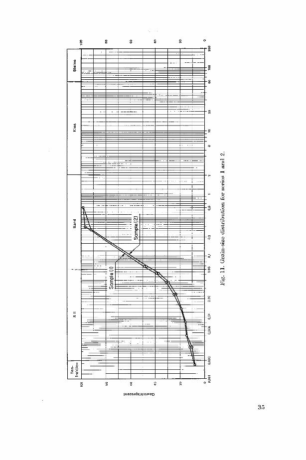
— Grain-size distribution is given by the accompanying curves (Fig. 11, 12

and 13), representing the various series.

From the curves we find that the components are:

Clay = 9—13 %Silt = 35—31 %Sand = 56 %

The detailed percentages of various diameters can be seen from the curves.

— Proctor curves: (Fig. 14 and 15), are given for the various experimentalseries. Fig. 14 shows the standard compaction curve for series 1, 2 and 3,

whereas Fig. 15 gives it for series No. 4.

— Carbonate content = 49.50—50.50 %.

b) Effect of colloid on the volume-weight of the soil

It was aimed to take a wider range of ye*, or yd in series No. 3, varing from

1.70 to 2.10 t/m3, calculated for the same water-content and different soil

dry-weights, so as to give a certain volume of soil and water mixture. This

volume is that of the soil container in the apparatus. But it was found that

the values of 1.70 t/m3 and 2.10 t/m3 could not be attained in practice. For

this reason, this phenomenon had to be examined to decide the working range

of the material.

Several experiments were made using the soil cylinder of the apparatuswith a volume of 48 000 cm3, calculating the soil weights for the same water-

content, but for various volume weights.The results showed that the upper limit for the values of yc*, in which the

calculated values coincide with those which are attained experimentally, is

34

2.

and

1series

for

distribution

Grain-size

11.

Fig.

200

100

60

02

00,01

0,006

0,002

0,001

11

0

IJ

—-

IJ

Itt

IJ

'

JfT

IJ

(2)

Sample

''i

1

IJ

1J

-

1(1

)Sample

IJ

/ iif

I1

-

[1v;

::-'

<<!

IfTT

Steine

Kies

Sand

Silt

fraktion

Ton-

3.

series

for

distribution

Grain-size

12.

Fig.

200

100

60

20

10

0,02

0,01

0,006

0,002

0,001

I0

jI

II

jI

I1

it1M

Tin

JI

Sample(2)

\it

11J

Iit

uJ

17

uu

If111

JI

/|]

||(1)

Sample

uJ

I'A

iff

Ifu

JIf

IM

IfII

Steine

Kies

Sand

Silt

fraktion

Ton-

OS

OS

*4

CO

4.

series

for

distribution

Grain-size

13.

Fig.

100

60

0,02

0,01

0,006

0,002

0,001

1I

Ji

J1

1I

1(2)

Sample

Ji

Urn

/

'V

Ji

e(0

Samp

JI

tfJ

iJj

Jjt

tf1

lM

II

Steine

Kies

Sand

Silt

fraktion

Ton-

Compaction Test

Labor-Nr. 11 190

Serie 1, 2 and 3

Material Kloten-Ziirich

Komponenten 0.0016—1 mm

Giinstigster Einbauwassergehalt 11.60 %

Entsprechendes Trookenraumgewicht 1.90 t/m3

Entsprechendes Nassraumgewicht 2.13 t/m3Spezifisches Gewicht 2.73 t/m3

Sattigungsgrad 86.00 %

Versuch Nr. 1 2 3 4 5 6 7

Wassergehalt Wa in % 9.4 12.4 15.4 18.4 21.4

Gewicht-Probe + Zylinderin Gr. 3985 4040 4007 3962 3928

Gewicht d. Zylinders in Gr. 2123 2123 2123 2123 2123

Gewichtd.Probe ff*inGr. 1862 1917 1884 1839 1805

Endwassergehalt We in % 9.72 12.4 15.4 18.4 21.2

Nassraumgewicht

G*/V in Gr./cm3 2.07 2.14 2.13 2.03 2.00,

:

Trookenraumgewicht

1.89 1.90 1.84 1.72 1 66V(i + we)m^T-'crn

5 2CD

e

1 1 0 1 5 Water¬ content %

Stempelgewicht 2500 Gr.

Zylindergewichf 2122 Gr.

Fallhohe 30.50 cm

Schlagzohl/Schicht 25

Schichten 3

Zylinder i 10

Volumen der gewogenen Probe cm3°c^.\

<V

uo,^u

MSi

s'*

100 %

90 %

80 %

s60 % 70 %

20

Wassergehalt in %

Fig. 14. Verdichtungsversuch.

38

Compaction Test

Labor-Nr. 11 190

Serie 4

Material Kloten-Zurich

Komponenten 0.0014—1.00 mm

Gunstigster Einbauwassergehalt 12.50 %

Entsprechendes Trookenraumgewicht 1.88 t/m3

Entsprechendes Nassraumgewieht 2.12 t/m3

Spezifisches Gewicht 2.71 t/m3

Sattigungsgrad 84.00 %

Versuch Nr. 1 2 3 4 5 6 7

Wassergehalt Wa m % 7 7 12 7 11.7 16.7 18.7

Gewicht-Probe + Zylmderm Gr. 3895 4027 4050 3990 3950

Gewicht d. ZylmdersmGr 2122 2122 2122 2122 2122

Gewicht d.Probe G'mGr 1773 1905 1928 1868 1828

Endwassergehalt We in % 7.8 12 7 11.7 16.9 18 7

Nassraumgewieht

G*/V m Gr /cm3 1 95 2.12 2 14 2.05 2.001

TrookenraumgewichtCr*

1 81 1 875 1 92 1 76 1.68v(i + we)mUTlom

10 Water-Content %

25

5Q>

6.20

E

o

I 5

Stempel gewicht "iOO Gr

Zylindergewicht 21 22 Gr

Fallhohe 30,50 cm

Schlagzahl/Schicht 25

Schichten 3

Zylinder <t 10

Volumen dergewogenen Probe cm2

h%>

s* v

5^s^t£

Si %>

100 %

90 %

SOI' 601 ) N3%

80 %

10

Wassergehalt in %

Fig 15. Verdichtungsversuch.

20

o

>

39

2.05 t/m3, so that the lower limit is found to be 1.90 t/m3. Whenever a lower

value than 1.90 t/m3 was calculated, a higher experimental resulting value

was found. On the other hand for higher calculated values than 2.05 t/m3, a

lower one is attained.

Two other methods were tried to check the same phenomenon, using an

oedometer of 50 cm2 cross-sectional area.

1. Using the -premizing method

The process already described was repeated using an oedometer instead

of the soil container, that is for a series of experiments beginning with 1.70 t/m3to 2.10 t/m3, for water-contents of 22.50 % and 15 %.

The curves given in Fig. 16 show the results obtained. The diagonal at 45°

is the line of coinciding values. The curves for the degree of saturation 8 %,and the porosity n for both cases are also given.

The attained values agree with what was found from the experiments with

the soil container.

2. Using a dry prepared soil and the water-content spread through a filter plate

In this method the dry soil is homogeneously laid out in the oedometer

cylinder in a very loose state, and the water content is added using a graduatedwater container terminating in a valve. The required amount of water is

allowed to percolate at the soil surface under gravity only, using a saturated

filter plate.For 22.50 % water-content the volume weight was found to be 1.90 t/m3

with water percolating upwards and 1.92 t/m3 with water percolating in the

opposite direction.

For this reason the range of the volume weight in series No. 3 was taken

as 1.90, 2.00 and 2.05 t/m3 respectively.As a result it can be said that the effect of colloid content governed the

volume weight, so as to be within a limited range. This is due to the forces of

attraction and repulsion between the soil particles.

During the past decade workers in the field of soil-mechanics have become

increasingly aware of the important role played by colloid science in developingand understanding the fundamental behaviour of colloids in soil. As a result

mainly of the work of T. W. Lambe, F. ASCE, of the Soil Laboratory of M.I.T.

the advances achieved through investigations of colloid activity have been

adopted and made intelligible to the soil engineer [11].The reader is referred to an excellent summary by Lambe [29] of the nature

of the forces between particles and their effect. References [30] and [31] also

40

2.0 2.1 2.2* _

Y, gm/cm3 os calculated

Fig. 16.

41

refer to this field. Trolioft [11] obtained a formula for the shearing strengthin relation to the colloid friction and intergranular friction. No attempt will

be made in this treatise to detail them, and it would be of value if an attemptwere made to explain in a detailed manner the above-mentioned phenomenain terms of colloid effect due to the forces between the soil particles.

3.2. Experimental advance

Preparation of material

The material was brought from Kloten in the vicinity of the airport in its

natural moisture condition, dried in Power-O-Matic mechanical convection

ovens at 105° C for the time sufficient to evaporate all the excess water. Bymeans of special ball-mills, the soil was ground so as to eliminate lump forma¬

tion only, which generally takes place in some parts, then sieved through5 mm sieves.

Finally the dry soil was well mixed and made homogeneous by the method

of quartering, and was then stored in special barrels in the material laboratorystores.

Determination of soil properties

Before beginning any experiment the moisture content, specific gravity,

grain-size distribution, Proctor curves and carbonate content were estimated

by standard laboratory experimental methods.

Mixing of soil

The soil-mixing machine in the laboratory is of the vertical cylinder type,with horizontal axial rotation in the opposite direction to the rotating shaft,

to which louver blades of the same height as the cylinder are fixed. The angular

velocity is constant and can be adjusted as required in steps. It has the follow¬

ing specification:Swiss made, Gustav Eirich, No. 7282 (1955), type SWG Fll, filling 50 1,

380 V, 3.2 A, 1.5 KW, cos # = 0.87, 1410 rpm, 50 HP.

Trials were first made to determine the best mixing method, because it was

observed that the water content of the mixed soil was always less than what

is added. This is due to the centrifugal force, which permits a part of the added

water to stick to the dry steel walls of the cylinder during rotation. Trials

were made with a slightly increased amount of added water, but without goodresults. A satisfactory method was to give the inside walls of the drum a very

thin film of water.

42

Stages of the experiments

1. The dry weight of the soil and the water weight to be added were cal¬

culated from the volume weight of each experiment and its water content, in

accordance with the programme and the volume of the soil container of the

apparatus. The mixed weights were calculated to be laid in a number of layers.2. The inner walls of the mixing drum were coated with a thin film of water,

the dry weight for each layer were added, mixed dry for five minutes at low

speed. The mixing water was sprayed regularly at the same rate, and both

were mixed for another five minutes.

3. Each layer was laid in the soil container successively, its upper surface

being smoothed horizontally and adjusted. A soil specimen was taken by a

stainless steel sharp-edged small boring cylinder for the evaluation of the

volume weight and the water content of the layer. The bore hole was filled

with kaolin and a very thin horizontal layer of kaolin was spread on the

surface, in order to follow the surface deformations at the end of every expe¬

riment by cutting the soil cylinder at a diametrical vertical section and takingoff one of the two halves.

4. When the end layer at the top was finished, the upper perforated circular

plate was adjusted with two extensometers at the two ends of a diameter,and the recording of settlement begun.

At the bottom there is another filter consisting of a layer of sand (0.5 to

1.0 mm diameter) of 2 cm thickness laid on a filter plate, under which the base

is equipped with drainage pipes. The toe of the pile afterwards bears in this

sand layer.5. After 24 hours the pile was statically driven downwards gradually under

G, G + Px, G + P%. . .,where P2 is greater than P1 etc., till the pile bears in

the sand. Records of soil heave were continued and the penetration of the

pile in the soil under each load was recorded. The load was then successivelyreduced to G + P, where P = 60 kg.

6. Strain-gage readings were taken for each measuring station, once under

60 kg, then under no-load, and the strain given by 60 kg was calculated.

7. The consolidation pressure discs were fitted in place. After fitting the

last disc, settlement and gage records were taken.

8. Recordings stated in stage 7 were continued until the extensometers

showed no excessive settlement (difference of readings in 24 hours not more

than 0.001 cm). The consolidation was then considered to be finished. Gage

readings were recorded.

9. Consolidation loads were removed, gage readings were taken, extenso-

meter records were continued until the elastic action of the soil heave was

finished, and the gage readings were recorded again. The load P was removed

43

and gage readings were again taken. The difference corresponded to the strain

due to 60 kg.10. The friction force between the pile and the surrounding soil was measured

by means of Amsler pressure apparatus and crane (Fig. 17). This force permitsthe calculation of the mean final frictional stress between the pile and the

soil. Initial friction stress was calculated from stage 5.

Fig. 17. Measuring the pile-soil friction

forces.

11. With the pile out of the soil, the gage readings were recorded. The

difference between the first gage reading of stage 9 and the gage reading of

stage 11, reduced by the value due to 60 kg. gives the strain due to the negativeskin friction force. Hence the force can be calculated.

12. With the pile in its place, four boring-pipes of length equal to the soil

thickness were statically and slowly driven down, their axes forming a vertical

plane through a diameter of the soil cylinder. The lower ends of the boring-

pipes rested in the bottom sand layer.These bores served to investigate the end properties of the soil at distances

of half the pile diameter and twice the pile diameter respectively, measured

from the surface of the pile-shaft.13. Bolts fixing the two halves of the soil container were unscrewed, the

pile was slowly removed by the crane, and a vertical section through the

perpendicular diameter to the boring-pipes was made by the wire-cutting

44

apparatus. One half was taken off and the deformation lines of the various

layers seen and the soil-section was photographed. A discussion of these

photographs will be given in Chapter 7.

14. Standard laboratory experiments to determine yd, We%, ye* and the

degree of saturation S % were carried out for each layer of the two boringsfrom one side of the pile shaft, whereas the final shear strength of the soil is

determined by the unconfined shear test apparatus (Farnell) for each layer of

the other two bores. For the latter bores it was aimed to determine rf byFarnell for the layers of one of them, and by the triaxial apparatus for the

layers of the other, but experiment \t showed that it as not possible to form

the triaxial specimen without disturbing the sample.For this reason rf was always obtained by the unconfined tests.

CHAPTER 4

Results of tests

4.0. Model experiment

Experiment No. 3 from series No. 1 is chosen as a model for all the readingsand results. Since it is from one side under maximum consolidation pressure

pc according to the programme and from the other side, it has the upper limit

of the compressible layer thickness H. Moreover, this experiment is one of

the various series of the experimental work. All the readings during the experi¬ment for the different procedure steps, as well as the initial and final results

of properties and drag-forces are given.For the other experiments, which were carried out in the same way, only

the initial and final results are tabulated.

4.1. Readings and results of the model experiment

1. According to the programme the experimental conditions were as follows:

pc = 3.0 t/m2, H = 60 cm

yd = 1.54 t/m3, y*= 1.90 t/m.3Wa = 22.50 %, 8 = 80 %

45

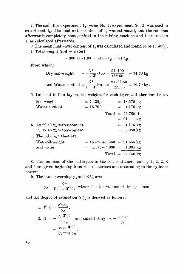
2. The soil after experiment 12 (series No. 1, experiment No. 2) was used in

experiment 13. The final water-content of 12 was estimated, and the soil was

afterwards completely homogenized in the mixing machine and then used in

13 as calculated afterwards.

3. The mean final water content of 12 was calculated and found to be 17.45%.4. Total weight (soil + water)

= 800-60-1.90 = 91 000 g = 91kg.

From which:

G* 91 100

Dry soil-weight =

^-^100 = -^^ = 74.30 kg

imi L L

G*„,

91-22.50and Water-content = -—= Wa =

—r^r^r-= 16.70 kg.

\ + W 122.506

5. Laid out in four layers, the weights for each layer will therefore be as:

Soil-weight = 74.30/4 = 18.575 kgWater-content = 16.70/4 = 4.175 kg

Total = 22.750-4

= 91 kg

6. As 22.50 % water-content = 4.175 kg.-. 17.45 % water-content = 3.080 kg

7. The mixing values are:

Wet soil-weight = 18.575 + 3.080 = 21.655 kgand water = 4.175-3.080 = 1.095 kg

Total = 22.750 kg

8. The numbers of the soil-layers in the soil container, namely 1, 2, 3, 4

and 5 are given beginning from the soil surface and descending to the cylinderbottom.

9. The laws governing ya and 8 % are:

G*

yd = ^rj-— ,where V is the volume of the specimen

and the degree of saturation S % is derived as follows:

1. W% = ^K,Yd

2. 8 =Y±K°k and substituting n =^^

nYw Ys

=

YsYaWX^

(Ys~Yd)Yw

46

From which:

Ydl-L.

w

10. Determination of the inital and final friction stresses between the pilesurface and the adjacent soil:

i.e. tp_s. andrp_sr

Calculation of p-h

This stress is always calculated from the penetrated depth of the pile under

its own weight only (own weight C? = 8.6 kg), directly when it ceases to move

further (see tables of consolidation and pile penetration), and the pile peri¬meter. This is to avoid the error arising from the relative movement between

the pile and the soil if rp_Si is calculated due to the penetration under G + Pf,where Pi denotes any load put on the pile to make it move statically further

downwards.

Example

Tp_s.for the model experiment 13

Penetrated depth under own weight G

Pile diameter 0

Pile perimeter = it0 = 3.1416-5

8.60

TP-St15.70-17

= 17 cm

= 5 cm

= 15.70 cm

= 0.032 in kg/cm2.

Calculation of rp

This stress is always calculated from the total final frictional force usingthe "Amsler pressure diaphram" and the final contact area between the pileand the soil.

Table 2 gives the calibration values of this diaphram.

Table 2

Dial reading in mm

Corresponding force in kg

0.849

100

1.697

200

2.552

300

3.401

400

4.248

500

Dial reading in mm

Corresponding force in kg

5.099

600

5.947

700

6.787

800

7.633

900

8.479

1000

47

Example,

Calculation of rp_s for the model experiment 13

Dial reading corresponding to total force = 0.300

Final friction force = 0.300-100/0.849 = 35.2 kg

Final depth = 58.0—4.891 = 53.109 cm

Pile perimeter = 15.70 cm

35 2•

t =:

= 0.042 kg/cm2.••

p~s' 53.109-15.708/

11. Readings of experimental procedure, initial and final properties and the

drag-force Fn for the model experiment:Table 3 gives the values of the initial properties of the soil. Table 4 gives

the readings and values of consolidation and pile penetration. The final soil

properties are given in Table 5, (Fig. 19, 20 and 21), whereas the representationof Fn for this experiment is given in Fig. 18. Table 6 gives the resulting Fnfor all experiments.

4.2. Results of remaining tests

The initial and final values of soil properties are given in Tables 7 to 21,

each two of which correspond to one of the remaining experiments.Table 22 gives the final mean values of soil properties at distances around

the pile of 1/2 the pile diameter and 2.0 times this diameter, each being measured

from the pile shaft. The mean of the mean-values for the whole soil cylinderare also given.

Note. The tables and figures of this chapter will be found on pages 48

onwards.

Table 3. Initial properties of experiment I3

(1.53) (22.53X79.25) (1.90)

H = 58.0. wt. denotes weight. Numbers between brackets are the mean values of

soil properties. * is not included in Wa % mean.

48

OS

L~

i>

t~

t~

t^

l>

r-

CO

mm

mm

Tt<*

*CO

CO

CO

CO

CM

IM

<M

<M

<M

(M

IM

rt

.—1

©

©©

IN

<N

oCN

©IM

©IM

CN

©©

oCN

©o

"tfCO

IM

IM

_,

rt

©©

IM

©CO

©©

lO

©o

•*

CN

©CM

©n

-*

oo

©©

o©

hDay

©o

CO

©CO

oCO

CO

©©

©CO

©©

CO

©©

©CO

©o

©©

CO

IM

©o

oo

Time

©o

©©

©©

©©

©©

©©

©©

©©

©O

oo

©o

©o

©©

oo

©a

++

++

++

++

++

++

++

++

++

++

++

++

++

++

++

++

CD

CO

CO

CD

CD

CO

CO

CD

CD

CO

CO

CD

CD

CD

CD

CO

CD

CD

CD

CO

CO

CO

CD

CO

CD

00

CO

TO

TH

CO

CN

i-H

©©

©©

,*,

©©

©O

©©

©©

©©

©©

©©

©r>

©©

oo

©©

©©

©o

©©

©©

o©

Cs

be

Hh

©o

O©

©o

©©

©©

o©

©o

©o

©©

©©

©©

©©

©©

©©

oo

©o

o©

o© ©

a.

a.

e.

a,

©H «

©©

©©

©©

©o

©©

o©

©©

©©

o©

©©

©o

©©

©©

©©

©©

oo

be

CO

CO

CO

CO

CO

CO

CO

CO

CO

CO

CO

CO

CO

CO

CO

CO

CO

CO

CO

o©

o©

©©

©©

©o

©©

©o

a.

53

"inCiH

cJh©

©©

©©

©©

©©

©©

o©

©o

©©

©©

o©

©©

©©

©o

oo

©o

o^

a

min

mm

in

mm

min

mm

mm

mm

min

mm

mm

in

mm

oTO

-*

tf

*CO

"tf<M

"©

©©

©CO

2Ph

00

TO

^H

on

CO

00

r~

©o

©©

t~

r~

t~

t-

t~

t-

t~

r~

r~

t-

t~

c~

t~

t~

t^

r--

r~

t~

t-

t~

r~

t^

t~

t~

r~

r~

-tf

CM

CO

CO

CO

00

O©

©©

©

cal©

©o

©©

©©

©©

©©

©©

©o

©©

©©

©©

©©

©©

o©

o©

©o

©O

©o

©©

s„0

OCD

mm

mm

mm

mm

mm

mm

mm

mm

min

to

mm

mm

in

TO

lO

TO

T*Htf

tf

CO

CO

<M

+£

fc_j-

ft

CO

CO

CD

CD

CO

CO

CD

CD

CO

CO

CD

CD

CO

CO

CD

CD

CO

CO

CO

CO

CD

CO

CO

CO

CO

CD

oq

©lO

-N

00

CO

^H

-+

4J

+J

Noto

©o

©o

©©

©o

©©

o©

©©

©o

©o

©©

o©

o©

or~

TO

CD

CD

©.-H

CO

CO

UIOo

©©

©©

©©

©o

©©

©©

©©

oo

©©

©o

o©

©©

©©

o©

©o

©O

o>>

>>

>.

-p

-U

-p

ationene-

mm

mm

mm

mm

m*

"tf*

Tt<*

<*

*tf

-tfCO

CO

CO

CO

CM

IM

o©

©

CM

CN

<M

CM

CM

CN

(M

CM

IM

©oo

CD

CO

<N

<N

^H

©©

©©

00

oGO

i-H

©©

©©

r-H

IM

CO

tf

CD

©©

Tt<©

be

-3CM

CM

CM

IM

CO

r^

r^

i^

r~

m10

CO

^H

r^

m©

^H

©r-H

©CD

o©

©in

lO

IM

r~

«)

lO

(M

CO

CO

©lO

<x>

©

UIO©

oin

mo

©©

©©

o©

©©

o©

oo

o©

©©

O©

to

©©

©to

©©

in

©to

mo

o©

tf

-tf*

tf

tf

T*ltH

tf

•tfCO

CO

CO

CO

CO

CO

CO

CM

CM

CM

IM

<M

<N

1—1

r"

©o

©©

""

-*

rt

rt

1—1

IM

""'

-*

©

CO

CO

CO

CO

CO

tX

tf

tf

tH

©00

CO

mCO

CO

CM

©©

©©

00

©©

m00

CO

©©

o—1

IM

CO

CD

©©

lO

o

mm

in

mCO

©©

©©

m©

©1—I

IM

©©

CO

mCO

IM

CO

>+

r~

©i^

lO

1—1

CD

r^

Tt<^H

1—1

i—1

CO

1—

IM

o

UIO©

©©

©o

04

IM

©©

©©

©©

©©

oo

©o

o©

©©

mo

©©

©o

lO

lO

©m

oin

©

efttens,

**

tf

tf

Th

tH

tf

Tf

•*

•*

Ttl-*

CO

CO

CO

CO

CO

CO

CO

CO

CO

IN

<M

l-H

©©

©o

t^

t~

1>

t^

t^

00

00

00

CO

T|HCO

^H

©t>

r~

t^

•tf-tf

tH

tf

CO

in

-tf00

©©

©©

(—1

i-H

(M

CO

CD

©©

lO

©

a»

§

00

00

CO

00

©©

©©

©in

IN

IM

IN

©00

©©

00

CM

.-H

l~

IM

CO

OS

i-H

oCO

<M

IM

©1^

r^

-tfIM

CD

oo

a

mm

r^

r~

©^

rt

©©

©m

©©

©©

©©

©©

©©

©©

CO

(M

©in

©in

in

©CO

©©

©CO

o

~£j

S

•M PI

pO

"* o S ooo

W^

X«

Oh

in

0)

<s

ou

S

a<z>

8ID

V

Ncnt

1No.Pild

8,8

8.o

a.

s

=1CO

as

CO

CS

^9

55

CO —l <M CO

OS 05 OS CSO IN CO T*cs cs cs cs

-2- 4be P

>o CO

© O OS c-

(N <N IN CO

©do©

O 00 mIN CM CO

odd

rp

d

^

£

is o h e

t> t> t> CDr-H i-H rH r—1

q CN <N CO

t-5 t-5 t~ CO

a .-

bo

IN OS O CO

oo r~ oo oo

O O -H hHH

OO 00 00 oo

* O CN *rP i-H r-H r-H

in ci ci ci

<N * <N t-

<n cm' cm cm

g Soildrywt. O lO Ol t-

CO CM © in

<N 00 -h CO00 t> 00 00

O O N ^in q q h

O CM* rP CO

00 00 00 CS

g Total drywt. CO T(< CO CO

CO * TH l>

l(j OJ M N

CO CO * -*CM CM CM IN

t> O * lO

© co © t~

>o d co io

CO * CO *« « N H

g Soilwetwt. HJ lO (N «

o * o oo

Tji d h CO,_, © —1 r-H

CM CM CM CM

o o e o

00 •* IN lO

i-5 co cm oo

IN IM cq H

g Total wetwt. CO tJI CO so

O CD <N O

t~ O CO COcd t-- t~ r-

CM CM CM CM

CO lO X ©CO CD CM CN

CO -H t^- r-H

CD t~- CD CO

CM <M (N r-H

rnw •

6o s -e

3 &

N OJ ^ fll

q h « h

CO r-H r-H din CO CD lO

CO lO IN rp

r- CM O CD

* OO id IN

to lO lO IO

Glass No.t- CO OS CMt~ 00 00 OSIN IN CM IN

OS T* 00 rP

in oo cs in

(N IN IN CM

Layer i—1 IN CO <* r-H CM CO TJH r-H CM CO "HH H (M M #

Bore O X

IN .SP-p AcS

*HP

d .9

cS

6-

o £CM %

a

IO rfi

eg

O o

10 0)

II aX o

o

X o

<s

* in

MHCO

0 o

HP

as II

HP©

HP CN

ft

o<S

X Tt<u a

oo

w

o

* 2a .

§ t*

.5'o oCD

ft IICC

-H •&cS m

"3©

I -

i—i to

> .*

CD

r=!H

50

1. Numbers between brackets deno¬

tes the gage-measuring positions.2. Max. ifn = 298kg.

Drag Force" Fn"-kgs. 300 200 100 0

Fig. 18. Representation of Fn for the model experiment I3.

51

kg/cm2.

0.029

=tj,_s.

properties,

soil

of

values

mean

the

are

brackets

between

Numbers

cm3.

31

=layer-specimen

each

of

volume

The

weight.

denotes

wt.

(80)

(22.50)

(1.535)

(1.9

2)58

=H

77

22.70

10.97

1.51

47.99

69.10

1.90

58.96

80.07

21.11

67

15

4

84

22.40

11.10

1.58

49.69

69.76

1.94

60.79

80.86

20.07

177

15

3

79

22.70

11.25

1.53

49.25

69.53

1.94

60.50

80.78

20.28

27

15

2

78

22.50

10.60

1.52

47.40

69.10

1.89

58.00

79.70

21.70

65

13

1

/o

/o

gg/cm3

gg

g/cm3

gg

gcm

SWa

wt.

Water

Yi

wt.

drySoil

wt.

dry

Total

*

wt.

wetSoil

wt.

wet

Total

wt.

Glass

No.

Glass

Height

No.

Layer

1\

experiment

ofproperties

soil

Initial

7.Table

6.

and

5Chapters

in

discussed

are

parameters

various

the

and

forces

drag

the

between

relations

The

087

184

207.5

124

195.5

298

194

121

KgS

mn—maximum

-FDrag-force

32

32

32

32

1No.

Experiment

43

21

Series

(Fn)

Drag-Forces

forc

esdrag

maximum

resulting

The

6.

Table

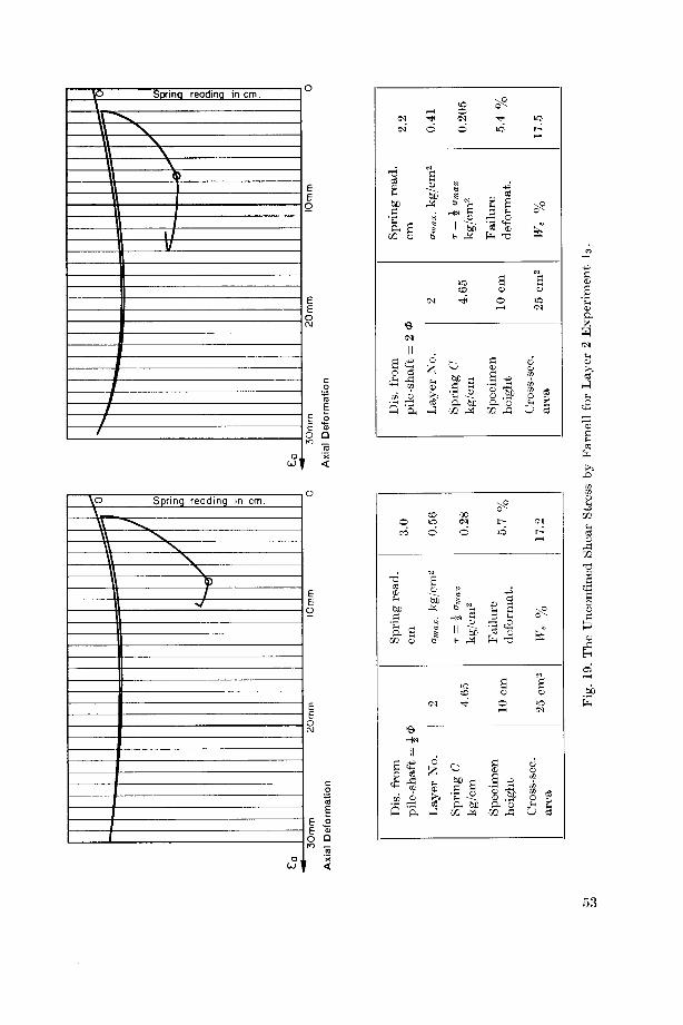
I3.

Experiment

2Layer

for

Farnell

by

Stress

Shear

Unconfmed

The

19.

Fig.

Oi

17.5

%We

cm2

25

area

Cross-sec.

%5.4

deformat.

Failure

cm

10

height

Specimen

0.205

kg/cm2amax

2=

T

4.65

kg/cm

GSpring

0.41

kg/cm2

max.

a2

No.

Layer

cm

<£2

=pile-shaft

2.2

read.

Spring

from

Dis.

17.2

%We

cm2

25

area

Cross-sec.

%5.7

deformat.

Failure

cm

10

height

Specimen

0.28

kg/cm2amax

2=

T

4.65

kg/cm

CSpring

0.56

kg/cm2

"max

2No.

Layer

cm

$\

=pile-shaft

3.0

read.

Spring

from

Dis.

10mm

mm

20

Deformation

Axial

30mm

010mm

mm

20

Deformation

Axial30mm

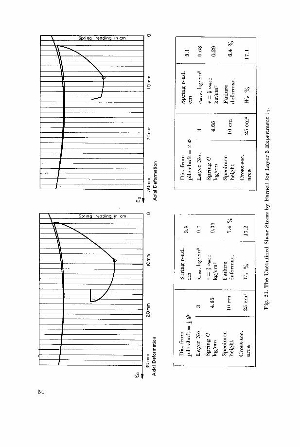
I3.

Experiment

3Layer

for

Farnell

by

Stress

Shear

Unconfined

The

20.

Fig.

17.1

%We

cm2

25

area

Cross-sec.

%6.4

deformat.

Failure

cm

10

height

Specimen

0.29

kg/cm2

4.65

kg/cm

GSpring

0.58

kg/cm2

Chi.

3No.

Layer

cm

2=

pile-shaft

3.1

read.

Spring

from

Dis.

17.2

%We

cm2

25

area

Cross-sec.

%7-4

deformat.

Failure

cm

10

height

Specimen

0.35

kg/cm2&max

^=

T

4.65

kg/cm

GSpring

0.7

kg/cm2

Omax.

3No.

Layer

cm

<t>

J=

pile-shaft

3.8

read.

Spring

from

Dis.

20mm

Deformation

Axial30mm

010mm

20mm

Deformation

Axial

mm

30

I3.

Experiment

4Layer

for

Farnell

by

Stress

Shear

"Unconflned

The

21.

Fig.

16.6

%We

8cm

height

Specimen

16.6

%We

8cm

height

Specimen

%3.5

deformat.

Failure

cm2

25

area

Cross-sec.

%3.5

deformat.

Failure

cm2

25

area

Cross-sec.

0.373

kg/cm2°max

^=

v

4.65

kg/cm

GSpring

0.41

kg/cm2Omax

^—

T

4.65

kg/cm

CSpring

0.746

kg/cm2

Omax

4No.

Layer

0.82

kg/cm2

Omax

4No.

Layer

4.0

cm

read,

Spring

=20

pile

-sha

ft

from

Dis.

4.4

cm

read.

Spring

<tJ

=pile-shaft

from

Dis.

10mm

20mm

Deformation

Axial

30mm

0

£o

10mm

20mm

Deformation

Axial

30mm

s

e

=1OS

00COOS

SQ ^9 © 00 OS OSOS 00 GO 00

r-l lO >0 i-l

OS OS OS OS

e

ea o

X X X 1©

CM CM CM O

©' © d ©

£ \0T* l-t OS ©

ffl OS t^ t-

CO Tj< CM Tt<

OS © OS t-

rt fl H H

ts

N

ao

"bo

o h co ost- t~ r~ t-

CO CM CO OSt~ t~ t~ t^

Soildrywt.

bo

CO © OS t-

CO lO t~ t-

CM CO CO OSE- t~ t~- t-

© CD i-h <Mi-4 © © OS

Trri (M *' oo

I- L- p- t~

Total drywt.

bo

t- OS CD t--J CM 00 Tjf

CO Ifl CO H

© OS OS ©i-l —1 i—1 CM

CM X OO CMOS OS h to

Ttl CM O OSOS OS OS OS

scj

"bo

lO ©CO l> 30 ©©©©r-4

IM CM' CM im'

t~ t^ OS ©© © © -H

cm' cm' cm cm'

Soilwetwt.

be

© OS lO GO30 CO * ©

IO CO QC 6© O © -H

CM (M CM (M

© CO CO CO

t-^ r^ os ©© © © —i

CM CM CM CM

Total wetwt.

be

-* GO CM GOCO -cH >0 t~

CD 00* 00 i-H

CM CM (M COCM IM CM CM

IM OO © COCM © CO t-

00 00 OS ©CM CM CM CO

IM CM CM CM

Glass wt. be

-* OS t~ ©GO I> © t-

© —I © -H

CM CM CM CM

CM CM t- ©00 OS CM CO

© © © ©CM CM CM CM

Glass No.CM CO t^ lO"-* ^ t- CD

H « ^ t^

CM lO CO lO

CC3 OS h n n -^ h n n t| i-H CM CO tH i-H <M CO Tfl

Bore9 -gcm be

© .SP

CO

<M ^

CS

56

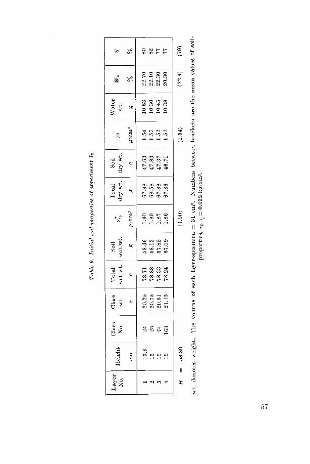
©1

kg/cm2

032

0=

tp-s

properties,

soil

of

values

mean

the

are

brackets

between

Numbers

cm3

=31

specimen

layer

each

of

volume

The

weight

denotes

wt

(79)

4)(22

(154)

(190)

80

58

=H

77

30

20

38

10

52

171

46

86

67

86

109

57

24

78

15

21

163

15

4

77

30

22

45

10

52

137

47

88

67

87

182

57

33

78

51

20

74

15

3

82

10

22

30

10

57

183

47

58

68

89

113

58

88

78

75

20

25

15

2

80

70

22

83

10

54

163

47

88

67

90

146

58

71

78

25

20

24

813

1

/o

/o

gg/cm3

gg

g/cm3

gg

gcm

SWa

wt

Water

Yd

wt

drySoil

v.t

dry

Total

Ye,*

wt

wetSoil

wt

wet

Total

wt

Glass

No

Glass

Height

No

Layer

I2

experiment

ofproperties

soil

Initial

9Table

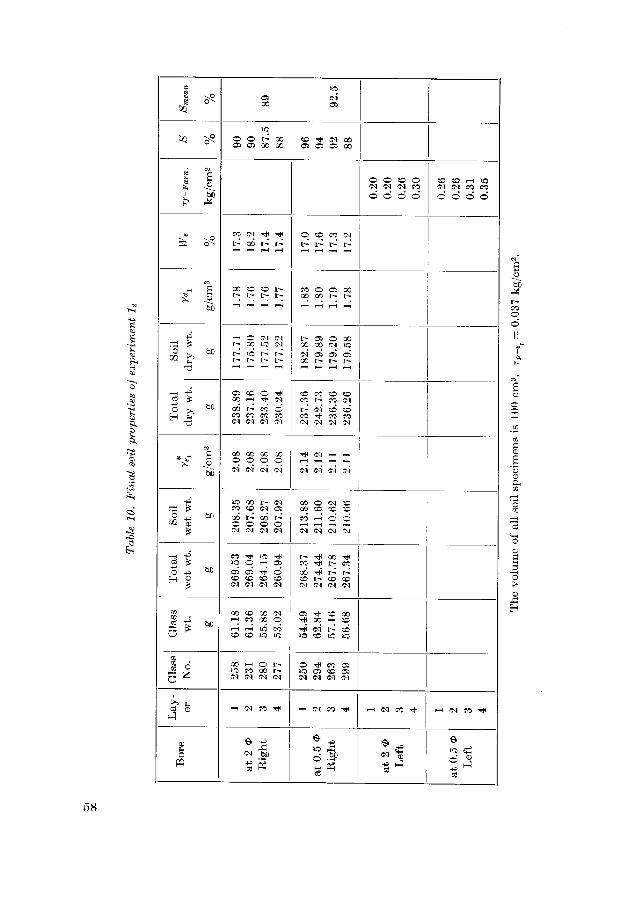
a

i^9o^

03

CO 92.5

SQ ^9o^

O O f- X03 03 X X

CO T* CM X03 C3 03 X

8

I

ao

"so"

O O CO oCM CM CM CO

<6 <^ o <6

CO CO rH lOCM IN CO CO

dodo

£ ^CO <N -# *

C~ X C-- t^O CO CO IN

t^ t^ t~ t-^

ao

~60

CO to CO t~

i> i> t- t-

CO O 03 XX X t- t~-

Soildrywt.

be

i—l © <N <Nt- CO lO <N

t~ »C t~ t~

t~ t^ E~ t~

l> 03 © XX X CM lO

IN 03 03 03X t~ F- t^

rH rH rH rH

Total drywt.

60

a to o -*cc i-H -* cm

CO t^ CO oCO CO CO COcm CM CM CM

CO CO CO toCO t~ CO CM

t- CM CO CDCO T* CO COCM CM CM IN

N

ao

~o2

X CO 00 QO

O O O O

<N ei in ei

Tfi 04 -H rH

OH CM IN CM

Soilwetwt.

60

io x r- (MCO CO CM 03

CO t-^ CO l>

o o o o« « N CI

213.88 211.60 210.62 210.66

Total wetwt.

60

CO -H- »C "HH

lO O rH 03

oi 05 -* dto CO CD COIN « IN O

(-* Ol H

CO -HH c- CO

CO * t^ t^CO l> CD COCM CM CM CM

Glass wt. 60

X CD X INrH CO X ©

rH rH lO CO

CO CO lO U)

03 tH CO X-* 00 rH CO

^ CM t^ CD

lO CO lO io

Glass No.X rH O t^

lO CO X t^

IN IN IN <N

O * CO 03lO 03 CD 03CM CM CM CM

CO CD

hirl IN CO Tjl rH CM CO TH rH IN CO "^ rH CM CO "^

Boreat

2

0

Rightat

0.50

Rightat

2

0

Leftat

0.50

Left

58

CO

kg/cm2.

0.030

=tp~s.

properties,

soil

of

values

mean

the

are

brackets

between

Numbers

cm3.

31

=layer-specimen

each

of

volume

The

weight.

denotes

wt.

(80)

(22.8)

(1.5

3)(1.88)

49.0

=H

78.5

22.80

10.81

1.52

47.23

69.45

1.87

58.04

80.26

22.22

165

16.66

3

82

22.90

10.95

1.54

47.68

68.11

1.90

58.63

79.06

20.43

61

16.67

2

78.5

22.7

10.78

1.52

47.23

69.56

1.87

58.01

80.34

22.33

26

15.67

1

/o

/o

gg/cm3

gg

g/cm3

gg

gcm

SWa

wt.

Water

Yd

wt.

drySoil

wt.

dry

Total

Ye0*

wt.

wetSoil

wt.

wet

Total

wt.

Glass

No.

Glass

Height

No.

Layer

2%

experiment

ofproperties

soil

Initial

11.

Table

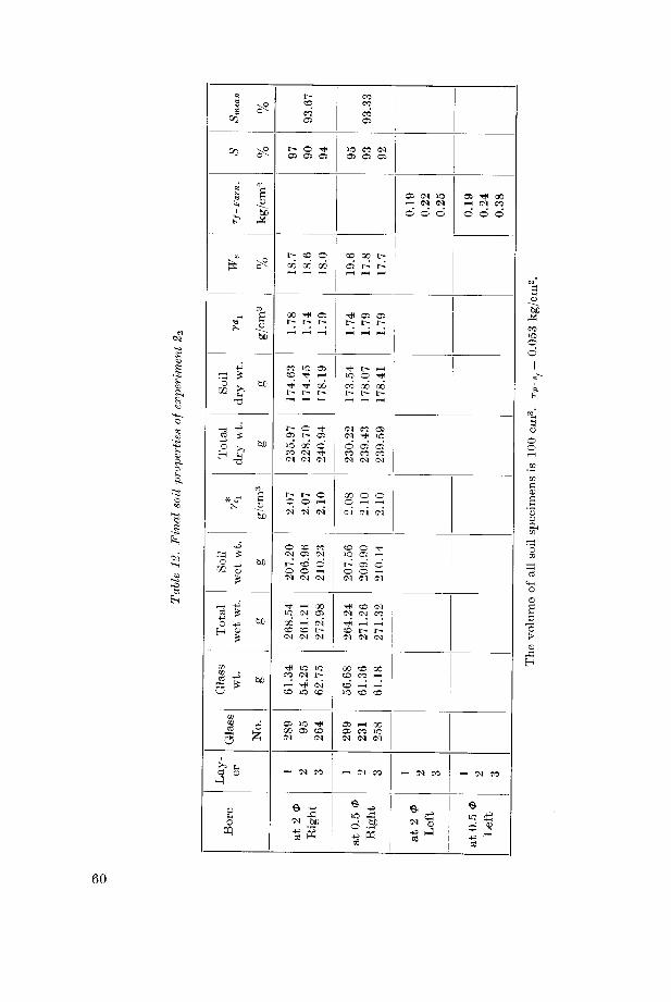
a.

fc<

e

93.67 93.33&5 C5^

t- o *a os os

lO CO CMOS OS OS

e

I

0]

1 OS CM "Oi—l CM CM

odd

OS * 00i-H CM CO

odd

£t- CO o

GO 00 00

CD 00 t>

d t- i>

o

~5o

00 -* OSt~ t~ t~

Tt< OS OSr~ r- t-

Soildrywt.

bB 174.63 174.45 178.19 173.54 178.07 178.41

Total drywt.

bX) 235.97 228.70 240.94 230.22 239.43 239.59* ^n

a-2"3d

t^ t^ o

q o h

cm <m' cm

00 o oO r-H i-H

<m' cm cm'

Soilwetwt.

be 207.20 206.96 210.23 207.56 209.90 210.14

Total wetwt.

be 268.54 261.21 272.98 264.24 271.26 271.32

Glass wt. bo 61.34 54.25 62.75 56.68 61.36 61.18

Glass d OS »a *00 OS COCM CM

O H CO

OS CO lOtN (N (N

CS o r-H <N CO i-H CM CO rH (M CO rH IM CO

Bore© -gcm be

3 Sat

0.50

Right <m T3

3J at

0.50

Left

oe

CO

o

d

oo

o

>

CD

X,H

60

kg/cm2.

0.042

=tv~s

cm3.

100

isspecimens

soil

all

of

volume

The

0.23

0.20

21

Left

00.5

at

0.23

0.20

21

Left0

2at

92.5

92

93

17.7

18.5

1.78

1.76

177.39

176.03

234.40

230.28

2.09

2.09

208.79

208.73

265.80

263.08

57.01

54.25

290

95

21

Right0

0.5

at

91

90

92

17.5

18.4

1.78

1.76

178.54

176.61

234.42

231.30

2.10

2.09

209.77

209.32

265.65

264.10

55.88

54.78

280

259

21

Right*

2at

/o

i^mean

/o

°/

S

kg/cm2

Tf-Farn.

/o

We

g/cm3

Yd,

g

wt.

drySoil

g

wt.

dry

Total

g/cm3

Ye,*

g

wt.

wetSoil

g

wt.

wet

Total

g

wt.

Glass

No.

Glass

er

Lay¬

Bore

2%

experiment

ofproperties

soil

Final

14.

Table

kg/cm2.

0.037

=tj,_s.

properties,

soil

of

values

mean

the

are

brackets

between

Numbers

cm3.

=31

layer-specimen

each

of

volume

The

weight.

denotes

wt.

(82)

(23.3)

(1.54)

(1.9

0)38.5

=H

78

21.7

10.42

1.56

47.66

68.58

1.88

58.08

79.00

20.92

153

19.00

2

86

25.0

11.88

1.52

47.16

68.05

1.90

59.04

79.93

20.89

89

19.50

1

/o

%g

g/cm3

gg

g/cm3

gg

gcm

SWa

wt.

Water

Yd

wt.

drySoil

wt.

dry

Total

Ye0*

wt.

wetSoil

wt.

wet

Total

wt.

Glass

No.

Glass

Height

No.

Layer

2s

experiment

ofproperties

soil

Initial

13.

Table

kg/cm2.

0.039

=tj,-,.

cm3.

29

=Volume

prop

erti

es.

initial

of

tables

the

of

notes

corresponding

the

to

conform

brackets

between

numbers

and

wt.

(93.4)

(22.8)

(1.6

3)(2

.00)

58

=H

96

96

96

86

93

23.0

23.1

23.1

22.8

22.3

10.84

10.96

11.00

10.83

10.63

1.64

1.64

1.65

1.58

1.64

46.87

46.89

47.33

47.41

47.70

67.54

67.14

68.70

68.73

68.53

2.00

2.00

2.01

2.00

2.01

57.71

57.85

58.33

58.24

58.33

78.38

78.10

79.70

79.56

79.16

20.67

20.25

21.37

21.32

20.83

34

24

83

32

176

13

13

13

127

54321

/o

S

/o

Wa

g

wt.

Water

g/cm3

Yd

g

wt.

drySoil

g

wt.

dry

Total

g/cm3

Ye0*

g

wt.

wetSoil

g

wt.

wot

Total

g

wt.

Glass

No.

Glass

cm

Height

No.

Layer

3^

experiment

ofproperties

soil

Initial

15.

Table

CSS

a,8

a

5~

9.

8

e lO

^4?o^

CM

a

SQ

CQ\P OS CM * CO o O CO CO CO

o^ 00 a a Oi CS Oi Oi Oi OS

£

a IO IO IO

B O hh •* IO CM -H CM CO

6i CO CO CO CO CM ^ ^# CO

f-on o o o o o o o o

o^

t> O M lO CO CO CO CM CM

fe CD CD CD CD CO 1 CO CO CO CD

i—1 p-H p-H p-H P-H

a O p-H ^4 IO CM p-H -* CD CO

00 00 00 00 00 | 00 00 00 00

beP-H ' ' 1 ' ' ' 1—1 p-H —< p-H p-H

-P ^ co o r- 00 t> co © ^

a & 00 00 t> o P-H IO 00 Ol t~

o . be 05 03 * lO CO | H (D » IO

GO t~ 00 00 00 00 CO 00 00

ti p-H p-i p-H rt PI r-t r-l "*

r—l -P CO O H N <M CO CM 00 o

Tota dryw p-H Oi OS t> CO CM IO CO

t* r-l -* CO <N CO | 00 OS OS CO

i—1 CO * -* * CO CO 00 CO

1-1 CM CM CM (N CM CM CM CM

Pi

s<M 00 t> OS

o O -* lO r—i CM CM "* CO CD

?.o

be CM CM <M (N CM CM CM CM CM CM

*

-p CD Tt< Tj< lO CO p—H CO CD tX 00

a ps t~ (N 00 t- 00 OS CO t- O i>

£lSoe -* O * IO p-l r-i p-h CO CO IO

O

is CM CM CM CM CM CM CM CM CM

i—i-*i 00 00 IO o O O CS CM CM t~

c8 fe

-P^

o <N O -* CO 00 CO ^ O p-H

be CO IO -# CO CM t- co cs o CD

H |CM CO » t> t~ CO CO (35 CM OS

'"H CM CM CM CM CM CM CM CO CM

a} CM T^ p-H lO * OS p-H CD 00 CS

Glas wt. beCO q cm co

IO C35 t--

•>*

d00

idt> CO CS

co id co

CO

dCM O lO lO CD IO >o oo o CO

1-1

cc

Glas No.CM 00 N O 1—1 o OS CO Tfl CM

CO OJ ffl ^ Oi 00 a o oi CO

CM CM <M CM CM CM rH rt

£ n<N CO * IO p-H CM CO T)H IO CM CO -* IO CM CO t« IO

HH

o *£ io X^£ IO £

0cm be

3Ed .SP

CO

dp3=3

be

©

d

oIO

<DpH

cS

o

I

ID

©o

CO

J3

CS

H

63

kg/em2.

0.042

=rp-s.

properties.

initial

of

tables

the

of

notes

corresponding

the

to

conform

brackets

between

numbers

and

wt.

(94)

(22.30)

(1.66)

(2.035)

60

=H

94

94

94

94

22.3

22.3

22.2

22.3

10.66

10.67

10.63

10.63

1.663

1.66

1.66

1.66

48.31

48.14

48.23

48.19

69.48

70.07

69.18

68.44

2.04

2.03

2.035

2.03

29

29

29

29

58.97

58.81

58.86

58.82

80.14

80.74

79.81

79.07

21.17

21.93

20.95

20.25

173

46

184

24

16.2

15.7

15.7

12.4

4321

/o

S

/o

Wa

g

wt.

Water

g/cm3

Yd

g

wt.

drySoil

g

wt.

dry

Total

g/cm3

Ye0*

cm3

Volume

g

wt.

wetSoil

g

wt.

wet

Total

g

wt.

Glass

No.

Glass

cm

Height

No.

Layer

33

experiment

ofproperties

soil

Initial

17.

Table

(35

8,8

a

8

a

scm

CI

CO

OS

SQ ^5«5 lO

IN * O f-JOl Ol C5 CI

IO IO

t> cq h h

Ol OJ CR Ol

Tf—Fam. so

~3j

CM * ^ t-

rt <N CM CO

©odd

IO IQ

CO t^ IO -^i-H I-H <N T*

©odd

h c>- O0 t^ N 1>

ci oi co o

oi t> t> I>

so

"So

00 IN © r-l

t- CO Q0 00

IO 00 O i-H

t> t> OS to

Soildrywt.

60

U IO O H

CI <N CO lO

h oi CO Ot> 00 t> 00

•* CI -* CI

t~ CO CO CO

ni i> * -h

t- t- Ol 00

Total drywt.

60

O CO O 00

q * oo co

m h in idCO ^ CO -^IN <N <N <N

IO 00 CO oo o * ia

IO Ol Ol OlCO CO "# CO

IN IN i-H IN

£So

"So

O CO O ^H

CM CM IN IN

CO CO

Ol Ol i-H IN

q o -< i-;IN (N (N IN

Soilwetwt.

be

00 i-H 00 CO

01 Th "O <N

oi n oi ho -H o ^H

IN 0<l CM CM209.63 209.63 110.99* 212.08

Total wetwt.

SO

O <M GO O

q co q i-;

cd oi -^ cdCO t- CD t^

Cl M N M

^ CM 00 CI

oo o r~ ^-i

d ^ id dt- r~ co t-

IN IN i-H CM

Glass wt. 60

IN rH O t-

© IN IO CO

cd d -^ -^IO IO IO CO

F-l Ol Ol -*

M M h H

H H -*' 00

CD CO IO IO

Glass No.[~ IN O "*1^ Ol IO Cl

IN IM N M

CO -* Ol i-H

GO CO IO CD

IN GM CM IN

3? nH (M M * r-< 0M CO -* i-H IN CO tH i-l CM CO *

Bore© -p

<N bC

3 « at

0.5*

Right at

2

*

Leftat

0.50

Left

so

"So

CD

O

OIO

0U

03

o

^

o

so

oo

&

o

,£3

Eh

65

kg/cm2.

0.10

=Tp_s.

cm3.

32

isspecimen

layer-

each

of

volume

The

properties.

soil

initial

the

of

values

mean

the

are

brackets

between

numbers

and

weight,

denotes

wt.

(74.71)

(18.90)

(1.6

1)(1.9)

60

=H

74.1

18.60

9.45

1.61

50.86

72.79

1.90

60.31

82.24

21.93

46

14.5

4

75.3

18.90

9.67

1.61

51.03

72.15

1.91

60.70

81.82

21.12

36

14.5

3

74.0

18.90

9.58

1.60

50.74

71.50

1.90

60.32

81.08

20.76

25

14.5

2

75.5

19.30

9.75

1.60

50.61

70.89

1.90

60.36

80.64

20.28

164

16.5

1

/o

%g

g/cm3

gg

g/cm3

gg

gcm

SWa

wt.

Water

Yd

wt.

drySoil

wt.

dry

Total

Ye„*

wt.

wetSoil

wt.

wet

Total

wt.

Glass

No.

Glass

Height

No.

Layer

4%

experiment

ofproperties

soil

Initial

19.

Table

CD

8

a,o

a.

£

4 87.32 91.125BQ ^9

io O n io

CD X x* co

X X X X

q "o "o io

ai o id aix co co x

Tf-Farn. so

"So

rH X CD »QrH IO X fNrH -H rH IN

© © © ©

X CO CO IOt~ co o ©rH fN CO CO

odd©

fe'o o o ©co q t~ co

X 00 00 00

o o o oo io q o

CD t> d t~

CO

sO

"ho

<N IN IN IN

l> t> t-- t~

CD X CD Oi

r- t- r-- t--

Soildrywt.

oc

t- X CO 03io q co t>

(N CO IN* COt~ t- r- r~ 178.11 178.61 176.59 181.23

Total drywt.

be

O ID * oIN IN rH IO

d d in co

CM CO CO CO

in n in n

CO CO CO o

q x q io

ei ci h oiIO CO CO CO

IN IN IN IN

V

CO

so

"So

Tt< >o IO »c

q q o o

fN IN IN (N

CO

X CD X fN

q qq h

IN IN IN IN

Soilwetwt.

be

* co co coH IN CD IN

* lO * do o o oN M N M

x x co co

IN X CO ©

x d x cn"O © © rH

CM fN IN 50

Total wetwt.

bo

C- "^ I— t~-

f; * 00 a

d in" >o idco co CO CO

IN IN IN IN

© © t- ©IN rH I> CO

in" -i x dX l> CO l>

IN IN IN CN

Glass wt. bo

CO X i-H ^H

CO hH (N t~-

CO l> d CD

»c »o »o »0

IN IN "* t-

03 IN -* IN

CO* rH © X

t~ co co *o

Glass No."O co cn e»

X CD CD OS

IN fN IN

<N X rH *^ io ca «

IN IN IN IN

CO q>

1-3H H IS * H M CO ^ rH IN CO -* rH IN CO "*

Boreat

2

0

Rightat

0.50

Rightat

0.5*

Left

©©

oCD

Oh

CO

VhO

CD

s

"3>

CD

r3H

67

experiment.

this

of

properties

soil

final

mean

the

includes

22

Table

kg/cm2.

0.85

=tp-s

cm3,

30,7

=*

except

cm3,

32

isspecimen

laye

r-each

of

volume

The

properties

.soil

initial

the

of

values

mean

the

are

brackets

between

numbers

and

weight,

denotes

wt.

(64.75)

(15.4)

(1.6

5)(1

.91)

60

=H

65

15.3

8.13

1.66

53.35

109.24

1.92

61.48

117.37

55.89

280

15

4

67

15.6

8.35

1.66

53.53

111.00

1.93

61.88

119.35

57.47

272

15

3

67

15.2

8.18

1.68

54.11

118.05

1.94

62.29

126.23

63.94

287

15

2

60

15.5

7.60

1.60

49.12

106.14

1.85

56.72*

113.74

57.02

290

15

1

/o

/o

gg/cm3

gg

g/cm3

gg

gcm

SWa

wt.

Water

Yd

wt.

drySoil

wt.

dry

Total

*

wt.

wetSoil

wt.

wet

Total

wt.

Glass

No.

Glass

Height

No.

Layer

4s

experiment

ofproperties

soil

Initial

21.

Table

00

CD

o

"8

e

se

-si

En

ciCM

e

Eh

Ea03

IN io IO

02 o CO 02 02 CO 1—1 r- cm

o >-* >-H O o ^H ^H © ©

* ^ § IN <N IN CM IN CM CM IN CM

gigs8 -3 g ft

IO •O IO

° "s x X IN X 02 IN IO ^H

© o *-* o © ^H ^H © ©

© -S.J2 ^

S -s £ ^ <N CM IN IN IN CM CM CM IN

o3

>g.i S3§ -3 g ft

OJ IN * 02 02IO_ © CO

o ^ ^ o o ^H ^H i-H ©

^ 03 ^ H«

CM CM IN <N CM CM CM CM CM

ECI03

lO IO IO IN CO t~

CO r~ CO Tt< ^H ^* * i—1 X• r^ <N IN CM IN CO CM CM fH

*• a

s o o O o o o © d ©

§ 3 g fto *

CO

CM <N

IO

CO *IO

Valuesof kg/c

^ IN CM CM IN CO CM rH ^1

S -s 5 e^ o3 -^

or

o o o o d © © © ©

©

© 3 g ftr~ o r~

>o CD CO IO

IO ©i—i CO CO IN IN CO CM IN CM

^ 03 +=^

© o o o o © o © ©

o IO © CO

""UBg]^;,_, ,_, CO CO

l>

CO

IO

IN

CM_

d <n

c>02 02 02 OS 02 02 02 X t-

i ©t~ o © CM

*4H

o s* g s.

S 3 5 ^ OS 02 CO

CO

CO

q IO

CM C<I

CO

1> ©

ValuesX X 02 02 02 02 02 X l>

1 ©

§3 g ft

h fl i ft1=5 c3 ^ -+n

IO <N

CO

CO

OIO

co

CO IN IN CO IN -* CO rt t*

02 02 02 02 02 02 02 02 t~

o IO O 02 O CO © * ©

£5WUB9J^

02 t~

CO

X

o

X CD

IO © IO

X *

i ©© o o o IO * © X ©

Cp 813 l£tH CD IN * 02 IO CO -* X

alueso X t~ t- X t~ CO L- X •*

a A g rg lO o o t~ o CO © © o

> 8 3 fl ft t^ CO o CO 1-1 CO tH CO CM

02 c~ r~ X X CD t^ 1— -*

IN CM CO

S3

T

<"U139J\[IO 02

X

CO

X

©X

IO IO

©

«.2§3

! 3 g ftio r^ t~ I> CM © (N CM

^ 3 t- t~ X t~ t~ X X t~ t~

O Cj

© -s g ftIO o

COr—t

CO

t~

CO

© X X

> t~ X X t~ t~ X X t~ E^

^ 03 "^hs

i -P

'C <* 6 03 N OT N m

o 2 £ CM CM CO CO rH •*

03

©

O

©

03> ©

T3 -p

3 a© .3

g T3eg ©

2 aS Q

©

Ti -p

fl ^

69

CHAPTER 5

Discussion of parameters and treatment of the problem by the

"jr-theory"

5.0. Discussions of relations between drag forces Fn and the different parameters

In the discussion of the linear function relations, <x denotes the intersected

value of the x- or y-axis, /S denotes the relationship slope, and /J' = 1/jS.

a) Fig. 22 gives the relation between Fn and the consolidation pressure pc.

Fn is directly proportional to pc, and the relation is of the form:

from which xPc is the value of Fn when pc = 0, i.e. the negative skin friction

force is due to the soil's own weight only.b) Fig. 23 gives the Fn, H relation, from which the relation could be written

in the form:

Fn = p'H(H-*H).

0,400

0,300

Y~ °-°

Fig. 22. Relation between Fn and pc

Fn t

pc t/m2

0.121

1.00

0.194

2.00

0.298

3.00

70

0,0 0,10 0,20

1,90

-tfH~58-

0,30 0,40 0,50 0,60 0,70

Hm

2,00

Fig. 23. Relation between Fn and H.

2,20 2,30 y*0 t/m32,10

1,63 1,73 1,83

y d-maximum = 1,87 t/m3

1,93

Fnt H m

0.124 0.385

0.1955 0.490

0.298 0.580

F„ t yd t/m3

0.184 1.66

0.2075 1.63

0.298 1.53

Fig. 24. Relation between Fn and ya

71

<xH is the layer thickness at which the drag force ceases to appear, and Fn is

directly proportional to (H — ocH).

c) Fig. 24 represents the Fn, yd relation which reads:

In this, the slope $yi has a negative sign and Fn decreases as yd of the soil

increases.

d) Fig. 25 shows that Fn is directly proportional to (Wa %—ocw), where aw

gives the minimum water-content, below which no Fn occurs for this kind

of soil.

0,500

0,400

0,300

0,200

0,100

0,00

,

O^--"

(

£w= 0,223

k-e^_

0,15 0,16 0,17 0,20 0,21

r*°V

Fig. 25. Relation between Fn and Wa %.

F„t

Wa %

0.00

0.154

0.087

0.189

0.298

0.225

0,22 0,23W0 %

5.1. Relation curves between Fn and each parameter

Each of the curves in Fig. 22, 23, 24 and 25 was treated by the method of

least squares, using the following two equations, which are derived for the

coordinate axes x and y, in which a is the intersected value on the z/-axis

and j8 is the slope of the relation to the x-axis.

andSigma (x yr) — ym Sigma x

0 =

Sigma x2 —m x\

(I)

(II)

72

where: yr = reading value on y-a,xis.

ym = mean ordinate.

xm = mean abscissa,

m = number of readings.x = reading value on £-axis.

.'. We find a and /? of each curve as:

a) Fn against pc

The relation is of the form Fn = <xPe + PPi!pc

Sigma (pc Fn) - F%m Sigma pcPp.=

Sigma p\~mp\

1.4035-1.2270 0.1765

14-3-4= 0.08825

and an =Fn -8npr = 0.2045-0.08825-2Pc 'I'm I Pe 1 ^m

= 0.2045-0.17650

= 0.0280 ton.

b) Fn against H

It can be written in the form H = xH + BHFn

Sigma (FnH)- Hm Sigma Fn

0 3178fiK — 0 SnOKzt 0 01739^

= 1.040.1424-0.1272 0.0152

and aH = Hm-fiHFnm = 0.4867-1.04-0.2058

= 0.4867-0.2140 = 0.2727,

which is about 5 times the pile-shoe height.

c) Fn against yd

The relation is of the form Fn = a. — Byd yd. The curve gives yd maximum

1.87 t/m3, at which value the negative skin friction ceases for this soil.

d) Fn against Wa %

The relation can be written in the form:

"a /o = xw + Pw ^%

Sigma Fn Wa% - WUm% Sigma FnPw =

Sigma F* - m F%m0.0832-0.0727

_

0.0105

0.0964-0.0494~~

0.0470= 0.223

73

and aw = Wam%-fiwFnm = 0.189-0.223-0.1283

= 0.189-0.0286 = 0.16 = 16%.

This is about 1.2 times the optimum water-content of the material used.

5.2. Boundary conditions of the negative skin friction forces

a) Due to the consolidation pressure pc

From section 5.1a and Fig. 22 we see that Fn = 0.028 ton when pc = 0. In

other words, the own weight of the unconsolidated soil exerts a force which

equals this amount on the pile by the negative friction acting on the pile

shaft; it is denoted as Fn_s.

Fn_s = "lJTp_sdZ= UHrp_Sm.o

Therefore Fn_s can be calculated as:

Fn_s = n0pileHrp_Sm = 3.1415-0.05-0.58-0.31 = 0.0282 t.

This is the same value given by the Fn — pc curve (see Figure 22).

b) Due to compressible layer thickness H

When H approaches about 5 times the height of the pile shoe, the negativefriction ceases to appear.

c) Due to the dry volume-weight of the soil

If the value yd which is equal to ys (l—n) is more than 1.87 (1.90 t/m3),the pile becomes a positive friction pile, i. e. the soil takes a part of the pileload instead of hanging on it.

d) Due to the water-content of the soil

From 5.1 d, it is seen that the water-content of the soil played a remarkable

role in the negative friction force, and it began to work if the water-content

was greater than the optimum for the soil used (more than 1.2 times the

optimum).

74

Conclusion

Therefore it could be said that, for this kind of soil, if:

H is less than or equal to 58;

yd is greater than or equal to 1.90 (t/m3);

Wa % is less than or equal to 1.2 times the optimum;

there are no drag forces for the system of bearing piles considered here.

5.3. Treatment of the problem by the "jr-theory"

In this paragraph, the treatment is given directly. If any further details

concerning the dimensional analysis and the Buckingham 77-Theory itself are

required, references [37, 38 and 39] may be consulted.

Let the drag force Fn be a function of:

ys,H,U,Pc and ^lA,Yd

.'. it can be written in the form:

\ Yd I

where:

ys = Specific gravitiy of soil.

H = Thickness of the compressible layer through which the pile pene¬

trates to bear in a good soil.

U = Pile-perimeter = -rr0pile in our case.

pc = Consolidation pressure.

A = Ratio between the soil weight/m2 and the consolidation pressure

= YdHIPc-

Wa % = Initial water-content of the soil.

yd = Dry volume-weight of soil.

In dimensional units:

Fn = f (t/m3, m, m, t/m2, Ac Wa % m3/t)

w.r.t. base dimensional units, where: M = mass, L = length, and T = time.

JPB = t =MLT-*

Vs = t/m3 = ML T-z/L3 = M L~* T~*

U = m = L

75

H = m = L

Pc = t/m2 = MLT~2\L2 = ML-1 T~2

Yd\°Wa%m*lt

Ac Wa % L3/J/ L T~2 = Ac JFa % if"1 Z,2 T2

taking the independent parameters to be:

(ys,Pc)

and the dependent parameters to be:

(h,u,*%&).According to the 7r-Theory:

where:

and

Solution

770 =&(TTlt1T2,ira),

^o= f(rs,Pc)Fn

"1 = f(Y,>Pc)H

^2 = f(Y*>Pc)U

"a = J(Ys,PcYd

T0 = f(y?,PVc0)Fn

.-. 7i0 = (M L~2 T-2fo (M L-1 T~2)y M L T~2

From M we get: x0 + y0 + 1 = 0

From L we get: —2x0- y0+l = 0

From T we get: -2x0-2y0-2 = 0

Adding (l) + (2) gives:— x0 + 2 = 0 i.e. x0 =-2

From (1) y0 =-3

._

KyI

Proceeding in the same way for n1

TT^fiy^p^H= (M L-2 T-2fi (M L l T~2)vi L

From M we get: xx+ ^ =0

From Z, we get: —2x1- ^ + 1=0

From T we get: -2^-2^ =0

(A)

(1)

(2)

(3)

(1)

(2)

(3)

76

Adding (l) + (2) gives:

From (2)

it, =

— x1+ 1 = 0 i. e. xx = 1

Vx =-1

Pc

Proceeding for tt2

Adding (l) + (2) we get

and from (1)

Proceeding for tt3

= (M L~l T-*Y* (M L-1 T-*)v* L

From M we get: x2+ y2 =0

From L we get: —2x2— y2 + l = 0

From T we get: -2x2-2y2 =0

— x2 + l = 0 i. e. x2 = 1

2/2=-!

^ys7T» =

Pc

^3 = /(yf> p?3)A^%

Yd

= (if L~2 T-a)*» (M L-1 T~*)v* Ac Tfa % il^1 L2 212

From M: x3+ y3-l = 0

From L: -2x3- y3 + 2 = 0

Froml7: -2x3-2?/3 + 2 = 0

From (1) +(2): -x3 + l = 0 i.e. x3=l

From (1) «/3 = 0

. . TT3 = .

Yd

Substituting in equation (A), we get:

(Hy. Uy, XWa%y\

Pc Yd

or F = i-^-0n

rl

pt/HUy! XWa%yPc Yd ')•

(1)

(2)

(3)

(1)

(2)

(3)

77

0,300

Fnt

0,200

0,100

0,00

pc vonoble & H constant.

0,116

0,120

4-/

/7-/

y/-E-

H vonoble & pc constant

= 0,98

A///0,15

0,08

0,100 0,200 0,300 0,400

P. • H • U t

030

0,20

0,00

0,000

Fig. 26.

Notations

Wq % Pi

r, rd

for yd- vonoble

for Wa% - variable

I-4—

//

//

U-

0,200 0,400 0,500

X - <^»o in ton

Fig. 27.

78

From the experiments the satisfactory solution is found to be the following

possible one:

Let: pcHU = 01

Fn = & (pcH U-XcWa0//°p3c).\ YsYd J

Wa%p*and = 0,

YsYd

Therefore the relation can be written in the form:

Fn = 0(01-\"0t).

Table 23 gives the relation Fn as a function of 0X, where pc is a variable

and H is a constant, whereas Table 24 gives the function where H is a variable

and pc is a constant. Fig. 26 illustrates the two relations, from which it is seen

that each of them is linear.

Table 23. pc variable and H constant

U = TT-0pue = 77-0.05 = 0.157 m

Series 1

Fn t

Pc t/m2HU m2

pcHUt

0.121

1

0.09106

0.0911

0.194

2

0.09270

0.18540

0.298

3

0.09106

0.27318

Table 24. H variable and pc constant

Series 2

Fn t 0.124 0.1955 0.298

pc t/m2 3 3 3

H m 0.385 0.490 0.580

HU m2 0.060445 0.076930 0.091060

pcHU t 0.181335 0.230790 0.273180

Table 25 gives the relation Fn as a function of 02 >where yd is variable,

whereas Table 26 gives the function where Wa % is variable.

Fig. 27 illustrates the two relations for different values of c (c equal to 1,

2 and 3 respectively), from which we see that the relation between Fn and yd,

Wa %, both as variables, is linear for the case of c = 2.

79

o io to

©00 CO 00

CO •<* *o o o

d d d

10 o o

aoo oo to

<N CO -^w

-<d d d

^H CO toN <M to r-H

•e- CO CO -*

.-< * tH *

d d d

o o oo >o o

© to 00 CO

-* CO CO

1-1 -H M

T*< toto rH tD

CO (M CO CO

o o o

d d ©

* o00 Ol o

<M00 CTS r-H

^ o O rH

d d d

to IO INOS rH CO

^< IN CO CO

d d d

eo

* 1CO CO COr~ t- r-

P in" IN IN

lO 00 CO

IN IN <Na IN <N IN

o d d

CO CO co tolO to to

-p r~i rH i-H

o o o

tq a00

IO00 oW5 to

d d d

N

& £ CO CO CO

-p

IO

00 t^ <#e OS O 00

&h -13IN <N i-H

d d d

ft d ca co

CO CO CO

rQ

toCO

rO

CO

o IN IO

•&oo OS -H<

CO CO CO

o o o

d d ©'

IO o o

a00

IN <N oCM

s<d d d

i-H t- OS(N IN to to© CO t- o

/< •* CO CO

d d d

o o oo o CO

«• to t- CO

""*! rH OS

^ -H d

>o oto co to

CO (N CO CO

O o o

d d d

00 * OS

CM 00 o o-< O i-H r-H

d d ©'

to IN O03 IN CO

-*< <N CO CO

d d d

eoCO

t~ c~ ir¬

-P IN on' IN

IO OS -*IN oo >o

8 IN rH rH

fe d d d

CO CO rH IO>o to to

-P i-H i-H rH

o O O

tu a00

>o

O Oto to

d d d

N

& i[ CO CO CO

-p

00 !>

e OS °°_

6s -13 IN o o

d d

& o N 03

K £H ^

* -r)l ,X

80

CHAPTER 6

End formulae describing "JF„'

6.0.

In Chapter 5 the maximum drag force Fn was discussed with the various

parameters and was found to be the sum of two parts. One part is equal to

the negative force produced by the consolidation of the soil under its own

weight only (i.e. pc = 0), which is termed Fn_s; the other part is developed bythe effect of a consolidation pressure pc (greater than 0) acting on the soil

surface. Either Fn_s or Fn will take place in our practical problems, in the

case of negative friction ones. Furthermore, the drag force was treated bydimensional analysis and the 7r-Theory in the above-mentioned chapter.

In the present chapter an attempt will be made to formulate Fn from the

experimental results, as applied in practice so as to calculate Fn_s or Fn, in

which case both H and Wa % are greater than zero. The final equation of Fnmaximum can be written in the following form:

Where:

? - F

®2

(vcHU-k= PcHU,

wa%P*

YsYd

YsYa J n'.,+#(#!-

A = —— = dimensionless quantity

c = constant experimentally evaluated.and

6.1. Calculation of F„_s (drag force due to soil only, pc—0)

a) If the mean frictional stress between the pile-shaft and the surroundingsoil is known, Fn_s can be written in the form:

H

K-s = J Urp_sdZ = UHrp_Sm,o

where rp_Sm can be obtained experimentally by a laboratory test at the end

of the final consolidation of soil under its own weight, in which a pile of material

similar to the actual material is driven before consolidation begins.

81

Otherwise, it is found to be empirically equal to O.BO-TFarnea ijwamea = un~

confined compressive strength) of the soil sample which is previously consol¬

idated and drained under a consolidation pressure equal to yEH' (H' = the

soil depth over the sample level). This point will be further discussed in the

following chapter concerning the soil properties in relation to the negativeforces produced. Or,

b) If Tv-S is for some reason difficult to determine experimentally, this

force Fn_s can be calculated by using the method published by Professor

Leonardo Zeevaert (1960) in the proceedings of the first Panamerican Con¬

ference on Soil-Mechanics and Foundation Engineering, Mexico, Vol. Ill,

pp. 1145—1152 [35].Without repeating the mathematical treatment and differential equations,

we give the two equations which enable Fn_s to be calculated:

Ks = (v':h-pvH)~ (i)ft

and: pvH = J(l-e-*) (2)

in which: y"e = submerged volume-weight of the soil.

H = thickness of compressible soil layer.

prH = vertical pressure acting when the negative force is alreadyhanging on the pile.

n' = number of piles/unit-area.U = pile perimeter.m = Kotg0n' U.

In the above-mentioned equations the author stated that it is sufficient to

take K0tg&, as equal to 0.25.

Fn_s of the experimental work, which is found to be 0.028 ton (see section

5.1 a and Fig. 22), was calculated in accordance with Zeevaert using the method

of successive approximations, by means of the following expressions:

AFn__sZ=Urp_SzAZ (3)

z

and Pvz =Poz-n"L4Fn_sZ, (4)0

where: A Fn_s = the negative skin friction force at depth Z.

TPsz= the frictional resistance between the pile and the soil at

this depth Z.

The value calculated by this method is = 0.0282 t, which is the same.

82

6.2. End form of F„-equation

From the 7r-Theory, and considering the value of Fn_s, the final form of

the maximum drag force Fn can be written in the form:

Fn = Fn_s+0(PcH U-X<%Ml£) = Fn_s+0(01-X'=02),

or Fn-Fn_s = 0(01-X02)

i.e. Fn-Fn_s = K{a01-b\"0i),

where: a, b and c are constants determined from the treatment by the experi¬mental results.

Table 27 gives the values of 0X, A and <Z>2 and the constituents of each of

them.

Table 27

U

ys

Fn-

= 0.157 m

= 2.73 t/m3 for series 1, 2 and 3

= 2.71 t/m3 for series 4

= 0.0280 t

Exp.No.

Fn

t

Pc

t/m2

Pc3 H

m

4>! t =

PcHU

A =

Pc

Wa % ya

t/m3

ysya

02 in t =

Wa %P3c

ysya

li 0.1210 1 1 0.580 0.091 0.890 0.225 1.54 4.200 0.0536

12 0.1940 2 8 0.588 0.183 0.453 0.224 1.54 4.200 0.4270

13 0.2980 3 27 0.580 0.273 0.296 0.225 1.53 4.180 1.4600

22 0.1955 3 27 0.490 0.230 0.250 0.228 1.53 4.180 1.4800

23 0.1240 3 27 0.385 0.181 0.198 0.217 1.56 4.255 1.3700

32 0.2075 3 27 0.580 0.273 0.315 0.228 1.63 4.450 1.3850

33 0.1840 3 27 0.600 0.283 0.332 0.223 1.66 4.530 1.3300

42 0.0870 3 27 0.600 0.283 0.322 0.189 1.61 4.355 1.1700

Table 28 and Fig. 28 give the possible solution of the relation for the range

of experiments, from which the constants are:

k =0.416, a = 2.00,

b =0.70 and c = 2.00,

••• Fn = Fn_s + K (20,-0.70X10,)

Fn_s + 0.416 (2pcHU- 0.70 A2 a /o'Pc

\ 7s Yd )•83

Table 28

Exp.No.

Fn-F„-,

t

0i

t

2 0!

t

A2 0.70 A20.70 A2 02

t

2 01-0.70 A2 03

t

li 0.0930 0.091 0.182 0.794 0.5570 0.0290 0.1530

12 0.1660 0.183 0.366 0.207 0.1449 0.0620 0.3040

I3 0.2700 0.273 0.546 0.088 0.0618 0.0900 0.4560

22 0.1675 0.230 0.460 0.0625 0.0438 0.0648 0.3952

23 0.0960 0.181 0.362 0.0394 0.0276 0.0379 0.3241

32 0.1795 0.273 0.546 0.0998 0.0699 0.0968 0.4492

33 0.1560 0.283 0.566 0.1100 0.0770 0.1025 0.4635

42 0.0590 0.283 0.566 0.1040 0.0729 0.0845 0.4815

, 'IO250

/^

- /uf

—

0

I0 150

°

0,100/ °

0 050

^36 0,4 6

>m

0i = PcHU

02Wa%V3c

YsYi

A _

YaH

Pc

The final form is

Fn = i*Vs + k (a 0i- 6A« *2),

where: k = 0.416 a = 2.00

b = 0.70 and c = 2.00

0,00 0 40 0 80 I 60 2 00(2*, orox*f2)t

Fig. 28.

84

Table 29

ExperimentNo.

Fn-Fn-s

t

2<2>1-0.70A2<P2

tK A A*

li 0.0930 0.1530 0.610 + 0.19375 0.037700

I2 0.1660 0.3040 0.546 + 0.12975 0.016900

13 0.2700 0.4560 0.594 + 0.17775 0.031700

22 0.1675 0.3952 0.425 + 0.00875 0.000077

23 0.0960 0.3241 0.297 -0.11925 0.014330

32 0.1795 0.4492 0.397 -0.01925 0.000368

33 0.1560 0.4635 0.338 -0.07825 0.000612

42 0.0590 0.4815 0.123 -0.29325 0.086100

Sigma k 3.330

Km 3.330/8 = 0.41625

Sigma A2 0.187787

.187787

Experiment 4a is not included in this table because the pile became a positive-friction one.

K = (Fn-Fn-s) / (2#i-0.70 A2*2)

A = K—Km

-,/Sigma A*/0.1877I

<Pm = mean relative error = 1/ —~ — =\ „ _

r n (n— 1) r 8-7

= (0.333J1/2.10-1 = ±5.76 %

^065= (*m/iCm)-100

0.0576

0.41625

13.75 %

100

Table 29 gives the treatment by the method of least squares in order to

evaluate the error.

The foregoing determination of the constants, in which the value of c is

found to be 2, complies with what is found for c = 2 in the treatment by the

77-Theory of the experimental results illustrated in Fig. 27.

85

CHAPTER 7

Soil properties in relation to negative forces produced

7.0. Effect of pile movement and consolidation on the soil properties

a) General

The aim of the following paragraphs is to discuss the behaviour of the soil

through which the pile penetrates during the steps of pile movement and due to

the consolidation process. As the quantitative evaluation of the end-propertiesof soils in cases of negative friction are governed by the kind and originalconditions of the soil under consideration (mainly the relative density and

shear strength, which depends on the grain-size distribution, mineral composi¬tions, colloid action and many other factors), a generalised formula for these

end-values of the soil properties will be very difficult to obtain.

A discussion of the end-properties of the soil used will be given and illus¬

trated by the experimental results obtained.

b) Action of clayey soils under various types of pile loadings

Since any pile has a considerable volume, an equal volume of soil must be

displaced when the pile is driven, and the surface may be observed to heave

owing to the displaced volume of soil [10].This can be seen from the experimental tables given in Chapter 4, for

example for experiment 13.If it is assumed that the soil undergoes horizontal displacements which are

equal in all directions, the shaded element of soil BCDE on the horizontal

cross-section in Pig. 29 is suddenly forced to the shape represented approxi¬

mately by B' C D' E', under the large shearing strain which this figure indi¬

cates and there must be a considerable amount of disturbance to the soil

structure. The ratio between the two mentioned areas is mainly governed bythe pore-water pressure and the relative density of the soil; the areas may be

found to be equal when the soil has a critical density (the density at which

no volume change occurs) and is fully saturated. Whereas, if the relative

density is more or less than the critical one and the pores are over- or under-

saturated, the previously mentioned two factors accompanied by the gas

movement will determine the areas BCDE and B' CD' E', in which case the

latter area can be greater or smaller than the former.

However, the soil looses much strength at points adjacent to the pile, and

a relatively small amount of skin friction exists during driving. There may be

86

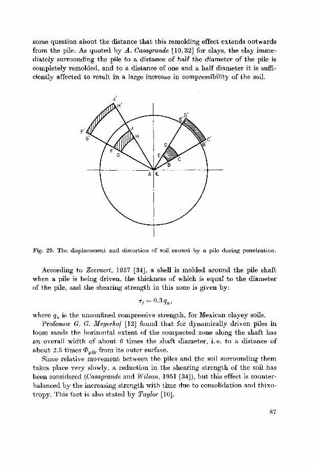
some question about the distance that this remolding effect extends outwards

from the pile. As quoted by A. Casagrande [10,32] for clays, the clay imme¬

diately surrounding the pile to a distance of half the diameter of the pile is

completely remolded, and to a distance of one and a half diameter it is suffi¬

ciently affected to result in a large increase in compressibility of the soil.

Fig. 29. The displacement and distortion of soil caused by a pile during penetration.

According to Zeevaert, 1957 [34], a shell is molded around the pile shaft

when a pile is being driven, the thickness of which is equal to the diameter

of the pile, and the shearing strength in this zone is given by:

rf= 0.3qu,

where qu is the unconfined compressive strength, for Mexican clayey soils.

Professor G. 0. Meyerhof [12] found that for dynamically driven piles in

loose sands the horizontal extent of the compacted zone along the shaft has

an overall width of about 6 times the shaft diameter, i.e. to a distance of

about 2.5 times 0pite from its outer surface.

Since relative movement between the piles and the soil surrounding them

takes place very slowly, a reduction in the shearing strength of the soil has

been considered (Casagrande and Wilson, 1951 [34]), but this effect is counter¬

balanced by the increasing strength with time due to consolidation and thixo-

tropy. This fact is also stated by Taylor [10].

87

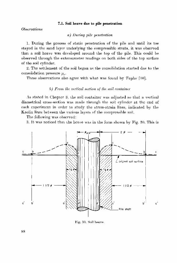
Observations

7.1. Soil heave due to pile penetration

a) During pile penetration

1. During the process of static penetration of the pile and until its toe

stayed in the sand layer underlying the compressible strata, it was observed

that a soil heave was developed around the top of the pile. This could be

observed through the extensometer readings on both sides of the top surface

of the soil cylinder.2. The settlement of the soil began as the consolidation started due to the

consolidation pressure pc.

These observations also agree with what was found by Taylor [10].

b) From the vertical section of the soil container

As stated in Chapter 3, the soil container was adjusted so that a vertical

diametrical cross-section was made through the soil cylinder at the end of

each experiment in order to study the stress-strain lines, indicated by the

Kaolin lines between the various layers of the compressible soil.

The following was observed:

3. It was noticed that the heave was in the form shown by Fig. 30. This is

Fig. 30. Soil heave.

88

Fig. 30-1. Strain line, pioductrt in i vperiment la- Fig. 30-2. Strain lines produced in experiment 2».

Fig. 30-3. Strain lines produced in experiment 3,. Fig. 30-4. Strain lines produced in experiment 4S.

89

accompanied by photographs of these sections, each of which represents an

experimental series of the programme.

It was found that:

a) The highest points of the heave (points a, a) occur at a distance equalto half the pile diameter from the outside surface of the pile shell, which

denotes the extent of the completely remolded soil.

b) A further distance of 11/2 times the pile diameter is sufficiently affected

by the pile movement.

4. Furthermore, it was noticed that, moving downwards from the soil sur¬

face, the strain lines abc tend to incline downwards to the horizontal instead

of being horizontal, in other words these lines bend up as they approach the

pile, which explains the negative friction forces.

7.2. Mechanism of soil heave due to pile penetration

Discussion

As regards the stress which produces the strains in the form of soil heave,

we must discuss the following important established facts:

1. During the penetration process of piles, as the rate of penetration is so

high, no consolidation can take place, and the soil in the path downward

moving pile is forced to displace.2. The displaced soil cannot be more than the volume of the pile itself

up to the plane on which the pile bears.

3. The displaced soil moves from the toe of the pile, and then upwards and

sideways so that a shell surrounding the pile and of a thickness equal to half

the pile diameter is completely remolded, and another shell outside it having

a thickness of l1^ times the pile diameter is sufficiently affected (see Fig. 30).

Mechanism of soil heave (Fig. 31)

1. As the two points "a, a" are the highest points of the soil heave, we can

assume that the cylinder a a'—a a' represents the surface of maximum shear

strain and consequently of maximum shear stress.

2. The shear along this cylindrical surface will be between soil and soil

along a definite surface, which is similar to the shearing process in a shear

box where the shear is forced to occur along a definite plane between the two

halves of the shear box.

3. The shear stress on the outer surface of this shell is transmitted to the

surrounding soil mass, and as the cylindrical surface enveloping the outer

surface of the shell increases in area as we move outwards from the pile, and

also as the transmitted shearing stress is constant, the shearing stresses on

90

Fig. 31.

these surfaces (and hence the corresponding shear strains) tend to get ever

smaller. This explains why heave fades away in moving far away from the

outer surface of this shell.

4. While the pile moves downwards, the body of the soil tends to move

upwards. This relative motion causes full mobilisation of the skin friction rp_s

between the shaft of the pile and the surrounding soil, which is in turn smaller

than rx on the surface a a' — a a'.

5. The pile circumferential stress rp_s downwards is resisted by rp_s on the

inner surface of the soil shell and by the shear stress tx on the outer surface

91

of the clay shell. These two vertical stresses result in the stress F, which is

nearer to the line of action of t1 as it is greater than rp_s.

This means that the action and reaction will not fall on the same line and

this will cause the element of the soil shell to be distorted as shown in Fig. 31c.

It also explains why the surface of the displaced soil ad is inclined towards

the pile.6. The value of rp_s, initial and final, as well as tx and t2 obtained by the

unconfined compression test (Farnell Apparatus), calculated as mean values

for the whole soil at a a' and bb' respectively, are tabulated in Table 30, from

which, if we compare the values of rp__s with t2, assuming that the soil is

homogeneous, we find that for the soil used:

which nearly agrees with the values given by Professor Zeevaert at the beginn¬

ing of this chapter.

Table 30

Series

No.

ExpNo.

Vari¬

able

Units

ofvari¬

able

Tp-, by Amsler app. TFarnel

Tp~Sf

Tp-St Tp-1, TlT2

kg, cm2T2

1 0.029 0.032 0.17 0.100 0.32

1 2 Pc t/m2 0.032'

0.037 0.30 0.240 0.16

3 0.032 0.042 0.31 0.266 0.16

1 0.032 0.042 0.31 0.266 0.16

2 2 H m 0.033 0.053 0.27 0.220 0.25

3 0.037 0.042 0.215 0.215 0.20

1 0.032 0.042 0.31 0.266 0.16

3 2 w t/m3 0.039 0.044 0.35 0.330 0.14

3 0.042 0.046 0.243 0.240 0.19

1 0.032 0.042 0.31 0.266 0.16

4 2 Wa % /o 0.100 No values

could be

determined

0.26 0.170

3 0.850 No values

could be

determined

0.20 0.175

92

7.3. Discussion of the end soil properties produced

The following properties were estimated by the Soil Mechanics standard

laboratory tests, each of which was calculated as mean values for the whole

soil at distances of half the pile diameter and twice the pile diameter, measured

from the pile shaft, and each of which was affected by the various parameters,

separately treated. Table 31 gives these properties as mean values.

These values are computed from the detailed results given in Chapter 4.

The curves of the changes in each of the properties with respect to each

parameter are drawn together.The above-mentioned properties are:

a) The dry volume weight of the soil (ydt/m3).

b) The end water-content We %.

c) The degree of saturation S %.

a) End dry-volume weight of the soil yd

Prom the end results obtained for each layer, for both the completelyremolded zone and the affected zone, it is found that the end yd increases

when we move inwards approaching the pile shaft and also with increase of

depth from the soil surface under the same consolidation load. Also, both

increase gradually if the load pressure pc increases. Pig. 32 illustrates these

results. Fig. 33 a shows the influence of the pile penetration plus the consolida¬

tion pressure effect on yd drawn as the resulting increment A yd against pc as

the variable in this series, for both zones. From the curves it can be seen that,

for a certain initial yd, as the pressure pc increases gradually, the soil particlesmove nearer to each other, causing an increase in yd. The rate of change of

A yd with respect to pc decreases gradually as pc assumes larger values, until

the soil grains come into contact (intergranular pressure), when they need

very high pressures to be crushed. This can be seen from the curves which

begin to approach a horizontal path. In addition it can be seen that the effect

at a distance of 20pile from the pile shaft is smaller than that at a distance

ofl/2<*Ve-Fig. 33 b gives the relation Ayd versus the soil thickness as a variable. It

shows that, for a soil of certain initial yd under the effect of a consolidation

pressure pc, A yd increases as the thickness of the soil layer increases until

this depth attains a limit at which the arch effect of the soil begins to act.

The rate of change of A yd\A H decreases, then as H increases again, this rate

of change begins to increase. Also the effect is greater near the pile shaft

than when we move outwards.

93

9,o

a.

S

a

6~~r~

CO IO m. ,

OS OS CO CO CO r-4 CO (M CM CO >

CQ 00 00 CO CD CO OS CO CO OS co CO'

^9 \P CO COcN io (N CM CO IO CM CM **• 1<*) ,_| CO CM <M (M CO eq <N -*t< CO CM

"J CO OS CO CO CO TO CO co CO CO CO

\P lO IO lO lO fH io

O^ (M <M CM T* CM t> t~

o OS CO CO o CM C5 CO * CO Tfl *

"J 00 1~ r~ t~ CO 00 t~ CO CO r- r- co

* o o

"1 IO 1^ t—t p-« r— t^ r-* CM o l-H CM lO

t^ r~ on GO r~ 1> 00 co 00 00 t~ l>

N

CO CO CO CO CO o CO

Xi-i IO <r> r-H ^ r- o l—1 * o r—4 00 io

Nr~ CO 00 00 r~ t- CC CO 00 CO t~ t^

CO -* CO CO CO * CO CO CD CO i-H IO

e IO 10 IO >o IO lO IO CO CO lO CO CO

N

^9 o o o o o io O ^ o o o o

-# CO <M CM * co CM lO CO CM IO CO

fe" 00 c~ t- t- CO i> O CO l> I> CO •*

^ ^° lO o o o r~ o o CO o o o ot~ CO o o CO l-H o CO tK o CO CD

kfe

OS t~ t~ t- CO 00 t~ CO t~ t~ t~ «*

"vp io >o W o lO o ocN o o (M CM r> o CM r> o CM o o

e

^

IO ">* T* -* oo CO <* 00 CO * CO Tf

(M IM IM IM IM CO IM IM CM CM CO IO

CM (M (M CM (M CM (M CM CM CM ri rt

lO lO IO r> <-> lO 10 lO

CO oo (M CM on CO IM <M i—1 CM IO i-H

o o i-H i-H o O HH ^H i-H r-H o o

(M (M (M CM CM IM CM (M CM CM CM CM

IO O lO

co (M <* •* CO CO "* ^H ^H »H O CO?.

>~o >—* |H i-H O O -^ hH *-H -H i-H O

CM !M IM CM CM CM CM CM CM CM CM CM

(M <-> O <-> <~> r> o r> -+ O O l-H

X05 OS CO Oi CO CO OS O o CO 03 CO

1-1 P-* rt rt rt ""* rt CM CM ^ r-H i-H

d 6rH (M CO rH <M CO CM CO i-H CM CO

co

shHH

0 a. S-tJ e

m fe

CDo

rt CM co *

w

ifl C

,fl ctjw ^3

0)

'£i-2'ft

Hi

A <D

+j H^

©

101

aTi

<s

0)TJ

'3,Jh

i-H0)

CI 0)

X

CI) ro

a 0)

MH,-

0 <+H

© iflCU

s ter<s as

aTlCO

<3TJ CD

.ctj n

cfl ^3

Was is

© to

-3 § -=;©

r> » h

Crf

MH

§ S 8a §1^ " cS

^3 ^3

CD I

R co o

a a -«

o 5 £O O cS

CO©

TJ

2 [3H >

94

, i yd t/nr.3

Distance from pileshaft in (»piie

Distance from pile

shaft in *piie

p = 3 t/m2

— = 2"

= 1

2 «

3e>

-f-;—I L

i volues of y

ii

-u.

Fig. 32.

95

(b) Ayd versus H (a)Ayd versus pc

1

0,25

0,20

0,15

0,10

0,05

yZ*//

"z*

+ Ay„ ,/mJ

0,30

0,25

1

l/z*^J

fzt

0,0 0,20 0,40 0,60 H m.

+ Ayd t/m3(d) Ayd versus WQ %

0,20

0,15

0,10

0,05

0,0 1,0 2,0 3,0

(c) Ay, versus yri

+ Ayd t/m3 'd '°

0,30 r

0,25

0,20

0,15

0,10

0,05

0,0015 16 I? 18 19 20 21 22 1,53 1,58 1,63 1,68

W0% yd t/m 3

Fig. 33.

1

0,25

.

I/2A

0,20

Izf,

0,15

0,10

0P5

\l/2«l

20N\S(

96

Fig. 33 c illustrates the relation between Ayd and initial yd as a parameterunder a constant pressure pc and soil weight. It was noticed that as yd increases,

the resulting A yd decreases, till we arrive a certain value of yd when no effect

can be seen. The final effect is also greater nearer the pile than further away

from it.

Fig. 33 d gives the same relation of Ayd but plotted against the originalwater-content. This curve illustrates the first part of the phenomena of mobilityof soil under moisture contents. When the moisture content is low, the soil is

stiff and difficult to compress. As the water content increases, the soil mobilityincreases. In other words, under a certain load the soil particles can easilymove to fill the voids and this results in an increase in the volume-weight.This goes on until the moisture content attains a limit above which the static

pressure of the liquid appears, and the grains suffer some resistance duringtheir movement, resulting in a small increase [36].

The curves also show that the effect is greater nearer to the pile-shaft. As

regards the permeability, it is found that this decreases as we approach the

pile, and also when we move downwards with the soil depth measured from

its surface. This result is obvious, since k decreases as the volume weight of

the soil increases, which is found to increase in the manner discussed before.

b) End water-content We %

Fig. 34 gives the relations between the various parameters and the rate

of change in the water content given as J W %. Following the same discussions

under a, we find that they apply equally to the A W % curves.

c) End degree of saturation S %

Fig. 35 gives the increase A 8 % against pc in curve 35 a. This curve can be

explained as follows:

For a soil having a certain yd and Wa%, as pc increases the particles move

nearer together, which results in a decrease in the porosity n. But the water

content decreases also. Therefore the rate of decrease of both n and IT % is

essential. Taking for example experiment 13, Tables 3 and 5, we find that:

__7s-Ya_ 2.73-1.53_

1.20_

'initial^ 2.13 2.73

/0'

2.73-1.81 0.92QQO/

2.73_

2.73-**/°'

A n = initial~

nfinal = 44 - 33 = 11 %

97

(b) AW% versus H (a) AW% versus pc

-aw% aw %

5,0

4,0

3,0

2,0

1,0 //

0,0I

15,0

4,0

3,0

2,0

1,0

0,0

1/2 0//

0,0 0,20 0,40 0,60 Hm 0,0 1,0 2,0 3,0

pc t/m2

(c) AW% versus W0%AW%

5,00

4,00

3,00

2,00

1,00

0,00

1

1/2 ill

'2 0

15 16 17 18 19 20 21 22 23 24 25 Wa%

Fig. 34.

98

+ AS%

24,0

20,0

(b) AS% versus H

16,0

12,0

8,0

4,0

,

'/2 *Afa

+ AS %

24,0,

20,0

(a) AS% versus pc

16,0

12,0

8,0

4,0

.

>/2 <£

^U

0,00 0,20 0,40 0,60 Hm. 0,00 1,0 2,0 3,0

PC t/m2

(d) AS% versus Wa% (c) AS % versus yd+ AS%

u+AS%

a

24,024,0,

20,0

16,0

12,0

8,0

4,0

0,0

,

15 16 17 18 19 20 21 22

20,0

16,0

12,0

8,0

4,0

0,0

,

^ y„t/nf.

1,53 ! 58 ^iii63',s\l 68*

-1,0

-2,0

Fig. 35.

99

i.e. -^- =i1= 1=33o/o

nfined 33 3

»n*AW°/o

-

W*%-We%_

22.53-17.10_

5.43_

WHnal%~ Weo/0-

17.10-

17.10-31"5/°-

In other words, the rate of decrease of n is more than the rate of decrease

of W %. This results in an increase in the final degree of saturation which

can be seen from Fig. 35 a.

Fig. 35b and d give the relation between the increase in the end degree of

saturation A 8 % versus H and Wa % respectively. They can be explained in

the same way as the curves for cases a and b.

For experiment 13, to compare the calculated Siinal % with that found experi¬

mentally (Table 22):

Smai% (from Table 22) = 93%

_

YsVdWe% 2.73-1.812-17.10

sHnai%> calculated{ys-7a)yw (2.73-1.812). 1

8592.8%.

0.918

Fig. 35 c, which gives the relation between A S % and yd, can be explainedas follows:

As yd increases, this means that the weight of soil material per unit volume

increases also, and under a certain consolidation pressure pc the effect on the

rate of decrease of the porosity n is less than that of the same pc on the same

soil having smaller ya. But owing to the increased weight of soil material, the

consolidation pressure and the action of gravity, the water has a greater

tendency to flow out. Therefore the end degree of saturation may decrease as

compared with its original value.

This can be explained, for example, through experiment 33, which has the

highest yd and pc limits of the programme (see Tables 17 and 18).

yd = 1.66 t/m3 and pc = 3 t/m2

-

2-73~1-66_

,

ninitial ~

2 7^~~

' °'

Id) -

2'73-L80_ ,iO/

nfinal 2 ^pile~

97Q—

/o >

Le- An = initial ~ nfinal = 39 - 34 = 5%,

An 5= — = 14.7°/ .

nfinal 34

Whereas: Wa% = 22.3% and We% =17.4%,

100

AW 4 9i.e. AW =4.9%, ^L = __27%.

This means that S % decreases for higher values of yd.

For experiment 33, to compare the calculated Sfinal with that found experi¬

mentally (Table 22) :

S % (from Table 22) = 92.50%

on/ n n , , , n2.73 • 1.80 • 17.50 86.4

_ nn,

8 %, final calculated =

(273_18Q)=

^^= 92.80%.

CHAPTER 8

Application

8.0. Calculation of a practical problem

The following example deals with an actual problem which is a typical one

for negative skin-friction of bearing piles, reference [15].

Data (see also Fig. 36)

Thickness of non-consolidated layer H

of which: H' = thickness above the ground water level

and H" = thickness below the ground water level

The ground water level is found to be depthThe volume-weight of H' = y'E = y*

Submerged volume-weight, of H" = y"K = y"e.-. yEH = y'EH' +y"EH" = 1.60-4.50+ 0.60-8.00

The total pressure at level — 8.50

(= 1.60-4.50 + 0.60-4.00)The initial pressure supported by the solid part of soil

.'. The pressure of consolidation at — 8.50 m = 6.6 t/m2

Compressibility

The coefficient of specific compressibility mvc

varies between: 1.20-10-4 cm2/gand 2.20-10"4 cm2/g

12.50 m

4.50 m

8.00 m

4.50 m

1.60 t/m30.60 t/m3

12.0 t/m29.6 t/m2

3.0 t/m2

101

Shear strength

rt = the initial shear stress of non-consolidated soil = 1.0 t/m2

Tf= the final shear stress of soil after consolidation = 2.0 t/m2

Pile properties

The pile cross-section is a square of dimensions = 0.4-0.4 m2

The pile perimeter ?7 = 40.4 = 1.60 m

The pile cross-section/ = 0.4-0.4 = 0.16 m2

Area concerning the pile F =5

of which the area affecting the negative skin friction

= (5-3W2 = (5-0.4)2 = 22 = 4

m'

m'

Filling

Compressibleloyer

t=0,60Bearinglayer

rf„i = 2

re=1.6

re=o,s

rF = i

*

Scale of Z+ 2,50

„.

i 0 5m

I—J I I—L

40x40cm*

Fig. 36. Corresponding to Fig. 4, 5 and 6 of reference (15).Calculation of curve II.

Filling (consolidation pressure)

Volume weight of fill = yfill

Thickness of fill

Intensity = pc = 2-2.5

The specific gravity of soil ys is taken to be the same as

for quartz sand

The following properties are found for each of the two

layers H' and H".

For layer 1:

Wa% = 28% and yd = 1.28 t/m»

For layer 2:

Wa% = 65 % and yd = 0.97 t/m3

= 2 t/m3= 2.5 m

= 5 t/m2

= 2.70 t/m3

102

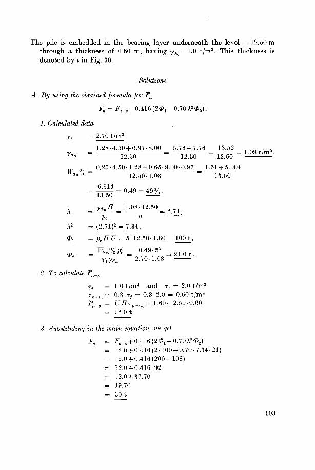
The pile is embedded in the bearing layer underneath the level —12.50 m

through a thickness of 0.60 m, having yEt= 1.0 t/m3. This thickness is

denoted by t in Fig. 36.

Solutions

A. By using the obtained formula for Fn

Fn = Fn_s + 0.416 (20,- 0.70 A2<Z>2).

1. Calculated data

ys = 2.70 t/m3,

1.28-4.50 + 0.97-8.00 5.76 + 7.76 13.52, _, ,

^=

12^0=

12.50 =I2T50=^^'

rlT n/0.25-4.50-1.28 + 0.65-8.00-0.97 1.61+5.004

am/0 12.50-1.08 13.50

6.614

13.50= 0.49 = 49%,

A „_

ydmH=

1.08-12.50^ 271

A2 = (2.71)2 = 7.34,

&± = Pr.HU = 5-12.50-1.60= lOOt,

* =Wk«=^49^==21.ot.tty*. 2.70-1.08

2. To calculate F,,n—s

ri= 1.0 t/m2 and T/

= 2.0 t/m2

t„ .= 0.3 • t, = 0.3-2.0 = 0.60 t/m2

i*L,= UHtv_s =1.60-12.50-0.60

n—s p bm

12.0 t

3. Substituting in the main equation, we get

Fn = 1,„_S. + O.416(2$1-O.7OA202)= 12.0 + 0.416(2-100-0.70-7.34-21)= 12.0 + 0.416(200-108)= 12.0 + 0.416-92

= 12.0 + 37.70

= 49.70

= 50 t

103

B. According to the theoretical method given by Messrs. M. Buisson, J. Ahu and

P. Habib, as given in section 1.2.2 of Chapter 1

To compare the obtained value of Fn, the same problem was solved bymethod B, as given by its authors:

The equilibrium equation of a pile is given by:

P + r + T,UZ-rfU(H-Z) = Qz B(l)

in which, using the notation of this treatise:

P = Load acting on the pile.r = The negative skin friction force as exerted by the fill weight.

Tf= Final shear strength of soil.

U = The pile perimeter.Z = The depth of the neutral point on the pile axis from the soil surface.

H = The thickness of the compressible soil layers.

Qs = Reaction of bearing soil.

From which the negative skin-friction force is given by:

Fn = r + TfUZ.

And r is given by the equation:

r=6>sinay/^t/, B (2)

where 6>sina is a constant = 0.30.

.". From equation B (2), we find r as:

2 502r = 0.30-2-^-—1.60 = 3.00 t.

tL "~~—"

To calculate -ry U Z, we must first determine the depth of the neutral point,i.e. Z.

The neutral point is given by the intersection of the curves I and II, each

treated separately (see Fig. 36). Thus:

Curve I. This represents the settlement of the soil with respect to the

increasing depth Z from the surface. It is determined as follows:

Considering a thin layer of soil of thickness d Z, in which the settlement

will be dy:

.". dy = AndZ,

where A n is the variation in the porosity.

»i ad e «..„ A p .

Also An =

\=

tt—T= mccdp,

(1+e) (1+e)lc L

104

where: e = The void ratio.

avc = Modulus of compressibility.A p = Pressure increment.

mvc = Modulus of specific compressibility.

.'. An =

-j~= mvcAp i.e. dy = mvcApdZ

d Z

H

or y =fmmApdZo

= The shaded area in Fig. 36 for each Z

equals the corresponding shaded area.

The values of y are given by Table 32.

Table 32. Calculation of curve I

B(3)

zArea

concernedm

Settlement

y

m 104 g/cm 10~4 cm2/g cm

0 140 1.2 168

2 103 1.4 144

4 74 1.6 118

6 49 1.8 88

8 24 2.0 48

10 8 2.2 18

Curve II. Illustrates the penetration depth of the pile as a function of Z.

a) To draw the curve Q, penetration of the pile for various values of Z:

1. Equation B (1) is written in the form (the author's equation 3, reference 15):

In equation B (4):

F = The area concerning the pile.

Tf= The final shearing strength of the soil.

K = Coefficient assumed to be a function of pile penetration only.

f = Cross-section of the pile. The other notation is as before.

In equation B (4), if:

Z = 0, pc = 0, r = 0

105

and Tf is replaced by ri, we get:

For the given numerical values, it will be found that [15]:

Q0 = 2.65Z.

2. If we choose arbitrary values for Q0 equal to Q0l> Q02. .. etc., then K

can be calculated.

3. Returning to equation B (4), Qz as a function of Z can be calculated

for each arbitrary value of Q0.4. Choosing the values of Z to be, for example 0, 2, 4, 8, 10... etc. in

meters from the soil surface, we can calculate Qz for each corresponding value

of Z.

Table 33

<3o

(trial)

t

K Qz

t

Values for Q in t for Z =

0 m 2 m 4 m 6 m 8 m 10 m

60

90

120

150

180

198

23

34

45

57

68

75

92- 4.7 Z

136- 7 Z

180- 9.2 2

228-11.7 Z

272-14 Z

300-15.4 Z

92

136

180

228

272

300

83

122

162

205

244

269

73

108

143

181

216

238

64

94

125

158

188

208

54

80

106

134

160

177

45

66

88

111

132

146

100 150 200 250 Load in t

-^^

UJUi1

tion

in

V \\ \ \_

toc \v \\\

1

Total[

w wv\V \\

Table 34.

z

m

Qz t y cm

P = 60t P=120t y 60 t y 120 t

0 23 83 0.25 0.60

2 36 96 0.30 0.75

4 49 109 0.45 1.00

6 61 121 0.60 1.30

8 74 134 0.90 2.05

10 87 144* 1.40 4.00*

2 = 10 8 Om

Kg. 37. This corresponds to Fig. 7

of reference (15).

* calculated at Z = 9.50 m

106

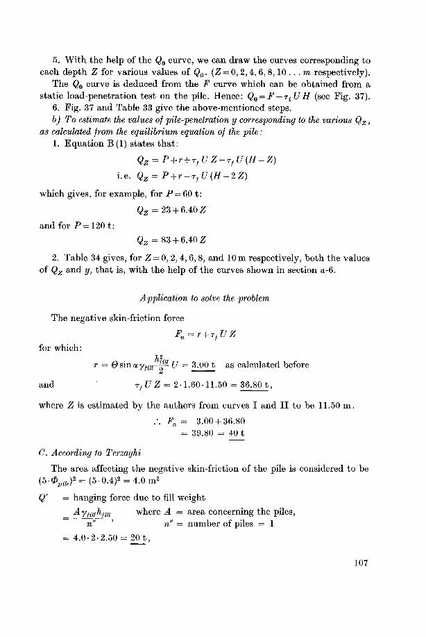
5. With the help of the Q0 curve, we can draw the curves corresponding to

each depth Z for various values of Q0. (Z = 0, 2,4,6,8,10 ...m respectively).

The Q0 curve is deduced from the F curve which can be obtained from a

static load-penetration test on the pile. Hence: Q0 = F —riUH (see Pig. 37).6. Fig. 37 and Table 33 give the above-mentioned steps.

b) To estimate the values of pile-penetration y corresponding to the various Qz,as calculated from the equilibrium equation of the pile :

1. Equation B(l) states that:

Qz = P + r + TfUZ-rfU(H-Z)

i.e. Qz = P + r-rf U(H-2Z)

which gives, for example, for P = 60 t:

Qz = 23 + 6.40 2

and for P=120t:

Qz = 83 + 6.40 2

2. Table 34 gives, for Z = 0,2, 4,6,8, and 10 m respectively, both the values

of Qz and y, that is, with the help of the curves shown in section a-6.

Application to solve the problem

The negative skin-friction force

Fn = r + rfUZfor which:

h2-r = 6 sin a ym-~- U

= 3.00 t as calculated before

and t,UZ = 2-1.60-11.50 = 36.80 t,

where Z is estimated by the authors from curves I and II to be 11.50 m.

.-. Fn = 3.00 + 36.80

= 39.80 = 40 t

C. According to Terzaghi

The area affecting the negative skin-friction of the pile is considered to be

(5-<Zyte)2 = (5-0-4)2 = 4.0m2

Q' = hanging force due to fill weight

Aymhm where A = area concerning the piles,n"

'

n" = number of piles = 1

= 4.0-2-2.50 = 20 t,

107

O" =

LH; where L = circumference, H = soil thickness,

t = shear strength of soil

= 8-12.50-1

= lOOt

Q" = hanging force due to soil, varies between 0 and 100 t

.-.Fn= Q' + Q"= 20 +(Oh-100)= From 20 t to 120 t

Fig. 38 shows the areas affecting the negative friction for one pile and the

various pile groups, as well as the representation of the area concerning the

pile in the example solved.

-(5)1 = 2,24m-

-\H

4

0,40 x 0,40

«-l,0n-

2,50= 1,0m

h- 1,12m -

The circles denote the piles.The areas included within the dotted lines represent

the horizontal areas which concern each pile or pile-

group, subject to the condition that the distance from

the nearest pile to the border of the mentioned area

(measured from the pile center line and denoted by a)does not exceed 2.50<Ppue.

Representation of the area concerningthe pile in the solved example.

Fig. 38.

108

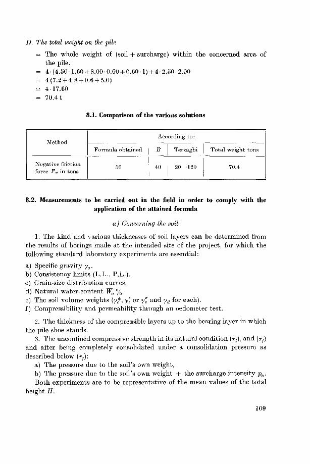
D. The total weight on the file

= The whole weight of (soil + surcharge) within the concerned area of

the pile.= 4-(4.50-1.60+ 8.00-0.60+ 0.60-1)+ 4-2.50-2.00

= 4(7.2 + 4.8 + 0.6 + 5.0)= 4-17.60

= 70.4 t

8.1. Comparison of the various solutions

MethodAccording to:

Formula obtained B Terzaghi Total weight tons

Negative friction

force F„ in tons50 40 20—120 70.4

8.2. Measurements to be carried out in the field in order to comply with the

application of the attained formula

a) Concerning the soil

1. The kind and various thicknesses of soil layers can be determined from

the results of borings made at the intended site of the project, for which the

following standard laboratory experiments are essential:

a) Specific gravity ys.

b) Consistency limits (L.L., P.L.).

c) Grain-size distribution curves.

d) Natural water-content Wa %.

e) The soil volume weights (y*, y'e or y" and yd for each).

f) Compressibility and permeability through an oedometer test.

2. The thickness of the compressible layers up to the bearing layer in which

the pile shoe stands.

3. The unconfined compressive strength in its natural condition (tj), and (t^)and after being completely consolidated under a consolidation pressure as

described below (t^):a) The pressure due to the soil's own weight,

b) The pressure due to the soil's own weight + the surcharge intensity pc.

Both experiments are to be representative of the mean values of the total

height H.

109

c) rp_s can be estimated with a laboratory test as already mentioned in

Chapter 6, or obtained as shown in Chapter 7.

b) Concerning the pile

The diameter or side length, as well as the shoe form and dimensions, so

as to permit the calculation of U.

c) Consolidation pressure

The consolidation pressure pc, as well as the area concerning the pile or

pile-group.

d) Moreover, it is preferable to know the shear strength and the cohesion

as given by the triaxial apparatus and the sensitivity of the soil.

CHAPTER 9

Summary and Zusammenfassung

A. Summary and conclusions

1. The effect of drag forces on piles produced by the settlement of adjacentsoil has been widely recognised in a qualitative manner for some time. Precise

quantitative information has been lacking, as a result of which cases of failure

have occurred or difficult and costly remedies have had to be executed. In

order to provide practical information about these forces on bearing piles a

laboratory study was carried out on a special model; a typical kind of loose

soil (silty sand with clay) was used with various soil properties and under

varying consolidation pressures.

2. The results are found to depend on the effect of two main sets of factors,

as follows:

a) The first one concerns:

The consolidation pressure (pc),The pile diameter (U), and

The thickness of the compressibile layer (H) through which the pile pene¬

trates to stand on a bearing strata.

b) The second set includes the soil properties, which are:

The ratio between the soil weight per horizontal unit area and the con¬

solidation pressure (yaHlpc), which is denoted by (A),

110

The natural water-content (Wa %),The dry volume-weight (yd) and

The porosity expressed by the specific gravity (ys) and the dry volume-

weight (yd).3. The greatest measured value of the drag force Fn is found to be propor¬

tional to the various parameters for the soil used as follows:

a) With repect to the consolidation pressure pc:

where a.Pc is the negative skin friction force due to the complete consoKdation

of the soil under its own weight only, i. e. pc = 0.

b) With respect to H:

Fn = fi'H(H-ocH)

where xH is found to be about 5 times the height of the pile-shoe, at the value

of which the drag force ceased to appear.

c) With respect to yd:

which states the inverse proportionality between Fn and yd.

d) With respect to Wa %:

K=ftw(Wa%-«w)

where aw gives the minimum natural water-content (about 1.2 times the

optimum), below which no Fn occurs.

4. The maximum drag force Fn which hangs on a bearing pile can be

computed from the following equation:

Fn = Fn_s + K(aVcHU-b\<=^^\ Ys/d

where the constants are:

k = 0.416, a = 2.0

b = 0.70 and c = 2.0

and Fn_s can be calculated by the use of one of the methods given in Chapter 6.

In the above-mentioned formula both H and Wa % are greater than zero.

5. To obtain the final form of Fn, referred to in section 4, the problem is

treated by dimensional analysis and the 77-Theory.6. The results of the experiments led to an explanation of the phenomena

of soil heave during pile penetrations.7. It is found that a cylindrical zone round the pile shaft of a thickness

of about half the pile diameter is completely remolded, on which surface the

maximum stress producing maximum strains in the soil takes place. Further,

111

that another outer cylinder of thickness 11/2 times the pile diameter is suffi¬

ciently affected by the pile movement to result in a large increase in com¬

pressibility of the soil.

8. The results show that the end volume weights increase when we move

inwards towards the pile shaft, and also with increasing depth from the soil

surface under the same consolidation pressure. In addition, the rate of increase

decreases as the consolidation pressure increases.

9. As an application, a practical problem was solved using the obtained

formula and, for comparison, it was also solved by the method mentioned in

section 1.2.2.

B. Zusammenfassung

1. Seit einigen Jahren ist der Einfluss der negativen Mantelreibung auf den

Pfahlen infolge der Zusammensetzung des anhegenden Bodens qualitativbekannt geworden. Um solche Probleme vollstandig zu behandeln, benotigtman bestimmte quantitative Informationen, die aber bis jetzt fehlen. Dadurch

traten in vielen Fallen Misserfolge ein, oder es mussten schwierige und kost-

spielige Instandstellungsarbeiten durchgefuhrt werden.

Die Resultate der vorliegenden Arbeit ergeben sich aus den Versuchen an

einem Spezialmodell eines stehenden Pfahles und einer geeigneten Labor-

methode. Dabei wurde eine typische Bodenart (siltiger Sand mit Ton) ver-

wendet, jedoch unter verschiedenen Zustanden und veranderlichem Konsoli-

dationsdruck.

2. In der wissenschaftlichen Untersuchung dieses Problems wurde die

negative Mantelreibung (im weiteren mit „Dragkraft Fn" bezeichnet) in

Abhangigkeit von den folgenden Hauptfaktorengruppen betrachtet:

a) Die erste Gruppe besteht aus dem:

Konsolidationsdruck (pc),

Pfahlumfang (U), sowohl

Machtigkeit (H) der zusammendruckbaren Schicht, durch die der Pfahl

eindringt, um auf einer tragfahigen Schicht zu stehen.

b) Die zweite Gruppe enthalt die Bodeneigenschaften, und zwar:

Das Verhaltnis zwischen dem Bodengewicht pro horizontale Flacheneinheit

und dem Konsolidationsdruck, (ydH/pc), welches mit (A) bezeichnet ist.

Anlieferungswassergehalt (Wa %),

Trockenraumgewicht (yd) und

die Porositat, welche durch (ys) und (yd) ausgedruckt sei.

3. Man hat festgestellt, dass die Proportionalitat zwischen der grossten

gemessenen ,,Dragkraft (Fn)" und den verschiedenen Parametern, fur die

verwendete Bodenart, lautet:

112

a) In bezug auf pc:

Fn = Xpc + PpcPc wobei (nPc die negative Mantelreibungskraft infolge der

Konsolidation des Bodens unter seinem Eigengewicht darstellt.

b) Betreffs H:

Fn = j3'H (H — a.H), wo ocjy die Schichtenmachtigkeit bedeutet, bei welcher

(Fn) aufhort. (<xH = 5 x Pfahlspitzenhohe).

c) In bezug auf yd:

Fn = a.Yd— PYdyd. Diese Beziehung stellt die umgekehrte Proportionalitat

zwischen (Fn) und (yd) fest.

d) Betreffs Wa % :

Fn = Pw(Wa % — <xw), wobei aH7(^l,2 Optimum-Proctor-Standard) der

minimale Anfangswassergehalt bedeutet, bei welchem Fn = 0 ist.

4. Fur einen stehenden Pfahl kann die maximale ,,Dragkraft" durch die

folgende erhaltene Gleichung ermittelt werden:

i, / tjtt

^^Wa%Pc\ wobei: k = 0.416, a = 2.0K = Fn-S + K[apcHU-bXc

a/olc, , A_A ,re ! s

\c

ysyd / 6 = 0.70 und c = 2.0

Das Bestimmen der (Fn_s) kann, je nach Zustand des Bodens, nach einer der

gegebenen Methoden in Kapitel 6 ermittelt werden. In der vorerwahnten

Gleichung sind H und Wa % grosser als Null.

5. Um die Endformbeziehung betreffs Fn aufzustellen, hat man das Pro¬

blem durch die 77-Theorie und die Dimensionalanalyse behandelt.

6. Die erlangten Resultate gestatten eine Erklarung fur das Phanomen der

Bodenhebung wahrend der Pfahleindringung zu geben.7. Man hat festgestellt, dass der Boden in einer zylindrischen Zone von

der Machtigkeit 0,5<PPfahl um den Pfahlschaft vollkommen gestort ist. Auf die

Aussenoberfiache dieses Zylinders wirkt die maximale Scherspannung, welche

auch die maximale Dehnung erzeugt. Ausserhalb der vorerwahnten Zone

befindet sich ein anderer Zylinder, dessen Dicke l,5<PPfahl betragt und insofern

von der Pfahlbewegung beeinflusst ist, dass deren Zusammendruckungzunimmt.

8. Die Versuche zeigen, dass bei einem bestimmten Konsolidationsdruck

das Endraumgewicht vom Rande des Versuchstopfes gegen den Pfahlschaft

zunimmt, ebenso wachst es an mit zunehmender Tiefe unter Bodenoberkote.

Bei steigendem Konsolidationsdruck stellt man eine kleinere Zunahme des

Endraumgewichts fest.

9. Als Verwendung der erhaltenen Gleichung von Fn ist ein praktisches

Beispiel gerechnet; daneben ist dieses Beispiel nach der Methode (1.2.2) zum

Vergleich gelost.

113

Bibliography

1. Chellis, S. D.: "Pile Foundations". McGraw Hill Book Co. Inc. New York (1951).

Chapter 16.

2. Terzaghi, K. and Peck, R. B.: "Soil Mechanics in Engineering Practice". John Wiley

& Sons. New York (1948). Chapter 9.

3. Russel, V. A.: "The Resistance of Piles to Penetration". E. & F. N. Spon Ltd. London

(1951). Chapter 4.

4. Krynine: "Soil Mechanics". McGraw Hill. New York (1947). Chapter 8.

5. Terzaghi, K.: "Theoretical Soil Mechanics". John Wiley & Sons. New York (1956).

6. Florentin, J. and ISHeriteau, O.: "About an Observed Case of Negative Friction on

Piles". Proceedings, Second International Conference on Soil-Mechanics and Foun¬

dation Engineering. Rotterdam, Vol. 114, pp. 371 (1948).

7. Moore, W. W.: "Expieriences with Predetermining Pile Lengths". Transactions

A.S.C.E. Vol. 114, pp. 357 (1949).

8. Caquot, A. et Kerisel, J.: «Traite de mecanique des sols». Gauthier Villars. Paris

(1956).

9. Lyon, T. L., Buchman and Brady: "The Nature and Properties of Soils". The Mac-

millan Company. New York (1959).

10. Taylor, D. W.: "Fundamentals of Soil-Mechanics". John Wiley & Sons. New York

(1956). Chapter 20.

11. Trollope, D. H. and Chan, C. K.: "Soil Structure and the Step Strain Phenomena".

Proceedings of A.S.C.E. (April 1960). SM 2.

12. Meyerhof, O. G.: "Compaction of Sands and Bearing Capacity of Piles". Proceedingsof A.S.C.E. SM 6 (December 1959).

13. Khalifa, M. K.: "The Failure Case of a Chimney". Proceedings of The Second Intern.

Conf. of Soil-Mechanics and Foundation Engineering. Rotterdam. Vila—30 (1948).

14. v. Oant, Edward and Stephens, J. E.: "Measurement of Forces Produced in Piles bySettlement of Adjacent Soil". Proceedings of Highway Research Board. Bulletin 173

(1957).

15. Buisson, M., Ahu, J. et Habib, P.: «Le frottement negatifo. Annales de l'lnstitut

Technique du Batiment et des Travaux Publics. No. 145. Paris (1960).

16. Haefeli, B.: „Die Pfahlfundation des Viaduktes von Travers". Problemes geotech-

nique dans le Val-de-Travers. Conferences tenues a la 2e Assemblee generate de la

Societe Suisse de mecanique des sols et des travaux de fondations. Neuchatel (1957).

17. Terzaghi und Frohlich: „Theorie der Setzung von Tonschichten". Franz Deuticke.

Leipzig und Vienna (1936).

18. Baver, L. D.: "Soil Physics". John Wiley & Sons Inc. New York (1959).

19. Jacoby and Davis: "Foundations of Bridges and Buildings". McGraw Hill Book Co.

New York (1941). Chapter 5.

20. Hetenyl, M.: "Hand Book of Experimental Stress analysis". John Wiley. New York

(1957).

114

21. Clark, D. S. and Datwyler, G.: "Stress-strain Relations under Tension Impact Load¬

ings". Proceedings A.S.C.E. V. 38, pp. 98, III (1938). A description of the first appli¬cation made by Simons of the bonded type of wire resistance gage.

22. Crandall, L. L.: "Electrical-resistance Strain-gages for Determining the Transfer of

Load from Driven Piling to Soil". Proceedings Second Inter. Conf. on Soil-Mechanics

and Foundation Eng. Rotterdam. V. 4, pp. 122 (1948).

23. Philips, A. 6.: ,,Technische Mitteilung". Fachschrift der Abteilung Industrie. Zurich

(1959).

24. Peekel: ,,Beschreibung und Bedienungsanleitung fur das elektronische Dehnungs-

messgerat Typ B 103 U. Rotterdam, Holland.

25. Miller: "Engineering". V. 17, pp. 174—176 (1924).26. McKay, G. A.: "Transactions A.S.C.E." Vol. 103, p. 220 (1938).27. Schnitter, G.: ,,Vorlesungen in Grundbau und Bodenmechanik". ETH (1957—1958).28. Meyer, Peter E.: „Vorlesungen in Grundbau". ETH (1941).29. Lambe, T. W'.: "The Structure of Inorganic Soil". Proc. A.S.C.E. Vol. 79. Separate

No. 315. (October 1953).30. Lambe, T. W.: "The Structure of Compacted Clay". Proc. A.S.C.E. Vol. 84. No.

SM 2 (May 1958).

31. Lambe, T. W.: "The engineering behaviour of compacted clay". Proceedings of

A.S.C.E. Vol. 84. No. SM 2 (V/1958).32. Casagrande, A.: "The Structure of Clay and its Importance in Foundation Engi¬

neering". Contributions to Soil-Mechanics. Boston Society of Civil Engineers (1932).33. Gamal Eldin, A. K.: "The Bearing Capacity of Piles in Relation to the Properties of

Clay". 5th Intern. Congr. of Soil-Mechanics and Found. Eng. Vol. II, 3 B/10, pp. 59/64.Paris (1961).

34. Corea, J. J.: "The Application of Negative Friction Piles to the Reduction of Settle¬

ment". 5th Intern. Congress of Soil-Mechanics and Found. Engin. Vol. II, 3B/7,

pp. 41/44. Paris (1961).

35. Zeevaert, L.: "Reduction of Point Bearing Capacity of Piles because of the NegativeFriction". First Panamerican Conference on Soil-Mechanics and Found. Engineering.Vol. Ill, pp. 1145/1152. Mexico, D.F. (1959).

36. Road Research Laboratories, H.M.S.O.: "Soil Mechanics for Road Engineers".H.M.S.O. London (1952 and 1957). Chapter 9.

37. Knapp, F. H.: ,,Ausfluss, Uberfall und Durchfluss im Wasserbau". Verlag G. Braun.

Karlsruhe (1960).38. Buckingham, E.: "Model Experiments and Empirical Equations". Transactions

A.S.C.E. Volume 37 (1915).

39. Selim, Yalin: ,,tJber die Bedeutung der Theorie der Dimensionen fur das wasser-

bauliche Versuchswesen". Karlsruhe, DK 626/627.001.5. Die Bautechnik, 36. Jahr-

gang. Heft 8 (1959).

115

Curriculum vitae

Born in Nag-Hammadi, Province of Kena, Egypt, 15th. July 1925. Mathe¬

matics matriculation, Egypt, June 1943. Practiced building construction by

a Building and Consulting Company 1943—1945.

Degree of B. Sc. Civil Engineering, Faculty of Engineering, Cairo Univer¬

sity, May 1950.

Employed at the Ministry of Public Works, Wadi-Elrayan Inspectorate,Research and Design Section, 1950—1951. Engaged by the Military Engineers

Corps, Department of Airports, Powerstations and Military Works, 1951—1954.

Then by the Municipality of Alexandria, Technical Departments, Soil-Mecha¬

nics, Foundations and Construction Inspectorate 1954—1957; from which he

practiced a year in municipal Civil Engineering Projects in Europe: France,

England, Holland, Germany and Switzerland.

From November 1957 to 1962, at the Swiss Federal Institute of Technology,Laboratories of Hydraulic Research and Soil-Mechanics, V.A.W.E., Zurich.