in-situ permeable barriers for reductive dehalogenation of

FINAL REPORT Development of Permeable Reactive Barriers (PRB)

Using Edible Oils

SERDP Project ER-1205

July 2008 Robert C. Borden North Carolina State University

Distribution Statement A: Approved for Public Release, Distribution is Unlimited

This report was prepared under contract to the Department of Defense Strategic Environmental Research and Development Program (SERDP). The publication of this report does not indicate endorsement by the Department of Defense, nor should the contents be construed as reflecting the official policy or position of the Department of Defense. Reference herein to any specific commercial product, process, or service by trade name, trademark, manufacturer, or otherwise, does not necessarily constitute or imply its endorsement, recommendation, or favoring by the Department of Defense.

i

TABLE OF CONTENTS

INTRODUCTION ......................................................................................................................... 3

1.1 RESEARCH OBJECTIVES ................................................................................................... 3 1.2 BACKGROUND.................................................................................................................. 4

1.2.1 Reductive Dehalogenation.......................................................................................... 5 1.3 PRIOR RESEARCH AND DEVELOPMENT ............................................................................ 7 1.4 REPORT ORGANIZATION .................................................................................................. 9 1.5 REFERENCES .................................................................................................................. 10

INJECTION OF NEAT AND EMULSIFIED EDIBLE OILS - RESIDUAL SATURATION AND PERMEABLITY IMPACTS............................................................................................... 13

2.1 INTRODUCTION .............................................................................................................. 13 2.2 MATERIALS AND METHODS ........................................................................................... 14

2.2.1 Injection Procedure .................................................................................................. 14 2.2.2. Emulsion Preparation............................................................................................... 16

2.3 NEAT OIL INJECTION RESULTS ...................................................................................... 20 2.4 EMULSION INJECTION RESULTS ..................................................................................... 21

2.4.1 Emulsion Transport and Permeability Loss ............................................................. 22 2.4.2 Mathematical Model of Emulsion Transport and Oil Retention .............................. 25 2.4.3 Effect of Clay Content on Emulsion Residual Saturation and Permeability Loss.... 27 2.4.4 Modeling Permeability Loss from Residual Oil ....................................................... 29

2.5 DISCUSSION ................................................................................................................... 30 2.6 REFERENCES .................................................................................................................. 32

ENHANCED REDUCTIVE DECHLORINATION IN COLUMNS TREATED WITH EDIBLE OIL EMULSION .......................................................................................................................... 35

3.1 INTRODUCTION .............................................................................................................. 35 3.2 ENHANCED REDUCTIVE DECHLORINATION IN LABORATORY COLUMNS TREATED WITH SOYBEAN OIL EMULSION........................................................................................................... 36

3.2.1 Experimental Methods .............................................................................................. 36 3.2.2 Experimental Results ................................................................................................ 38 3.2.3 Implications for Full-Scale Edible Oil Barriers ....................................................... 51

3.3 IDENTIFICATION OF SLOW RELEASE SUBSTRATES FOR ANAEROBIC BIOREMEDIATION.. 54 3.3.1 Experimental Methods .............................................................................................. 54 3.3.2 Substrate Screening Incubations .............................................................................. 55 3.3.2.3 Gas Production from SEFAs................................................................................. 62 3.3.3 PCE Biodegradation in Intermittent Flow Columns ................................................ 64 3.3.4 Implication for Field Application of Slow Release Substrates ................................. 66

3.4 REFERENCES .................................................................................................................. 67

TRANSPORT AND RETENTION OF EDIBLE OIL EMULSIONS IN AQUIFER MATERIALS ................................................................................................................................... 72

4.1 INTRODUCTION .............................................................................................................. 72

ii

4.2 EMULSION AND COLLOID TRANSPORT ........................................................................... 73 4.3 EMULSION TRANSPORT IN 1-D LABORATORY COLUMNS ............................................... 74

4.3.1 Materials and Methods ............................................................................................. 75 4.3.2 Experimental Results - Emulsion Transport in Columns.......................................... 76 4.3.3 Mathematical Model of Emulsion Transport............................................................ 81

4.4 EMULSION TRANSPORT IN 3-D SAND BOXES ................................................................. 83 4.4.1 Materials and Methods ............................................................................................. 83 4.4.2 Experimental Results ................................................................................................ 85 4.4.3 Mathematical Modeling of Emulsion Transport and Immobilization ...................... 91

4.5 MODEL SENSITIVITY ANALYSIS..................................................................................... 95 4.6 SUMMARY...................................................................................................................... 99 4.7 REFERENCES ................................................................................................................ 101

EFFECTIVE DISTRIBUTION OF EMULSIFIED EDIBLE OIL FOR ENHANCED ANAEROBIC BIOREMEDIATION.......................................................................................... 106

5.1 INTRODUCTION ............................................................................................................ 106 5.1.1 Perchlorate Extent and Degradation...................................................................... 106 5.1.2 1,1,1-Trichloroethane Degradation........................................................................ 107 5.1.3 Anaerobic Biodegradation using Emulsified Oils .................................................. 107 5.1.4 Field Pilot Test of Emulsified Oil Biobarrier ......................................................... 108

5.2 SITE CHARACTERISTICS AND BIOBARRIER INSTALLATION........................................... 108 5.3 MATHEMATICAL MODEL OF EMULSION TRANSPORT AND DISTRIBUTION.................... 112

5.3.1 Laboratory Column Study....................................................................................... 112 5.3.2 Field Validation of Emulsion Transport Model...................................................... 115

5.4 MATHEMATICAL MODELING OF CONTAMINANT BIODEGRADATION ............................ 119 5.4.1 Steady-State Simulations......................................................................................... 126 5.4.2 Full Scale Barrier Performance ............................................................................. 130

5.5 SUMMARY.................................................................................................................... 134 5.6 REFERENCES ................................................................................................................ 134

CONCLUSIONS......................................................................................................................... 139

iii

LIST OF FIGURES Figure 1.1 TCE and cis-DCE Biotransformation to Ethene in Microcosms Amended with

Semi-solid Hydrogenated Soybean Oil. Error Bars are the Standard Deviation of Triplicate Microcosms.

Figure 2.1 Grain Size Distribution of each Material. Figure 2.2 Cumulative Pore Diameter Distribution of each Material Calculated using Barr

2001) Procedure and Grain Size Distributions from Fig 1. Figure 2.3 Emulsion Droplets Produced with Different Surfactants and Mixing Devices as

escribed in Table 2.3. Figure 2.4 Cumulative Droplet Volume Distributions for Different Emulsion Preparation

Methods. Emulsion Numbers and Preparation Methods are Listed in Table 2.2. Figure 2.5 Variation in Hydraulic Gradient during Injection of Ottawa Sand with 3 pore

Volumes of Neat Soybean Oil Followed by Plain Water at Constant Flow Rate. Figure 2.6 Variation in Emulsion Concentration (C/Co) in Column Effluent and Effective

Hydraulic Conductivity during Injection of Field Sand with 3 Pore Volumes of Fine Emulsion followed by Plain Water.

Figure 2.7 Variation in Hydraulic Conductivity (K) during Injection of Concrete Sand, Field Sand and Field Sand + 3% Clay with Three Volumes of either Coarse or Fine Emulsion Followed by Water Flushing.

Figure 2.8 Comparison of Soo and Radke Model with Observed Variation in Relative Permeability when Concrete Sand and Field Sand are Flushed with 3 PV of Coarse or Fine Emulsion followed by Plain Water. Error bars Show the Range of Experimental Measurements in Triplicate Columns.

Figure 2.9 Variation in Oil Residual Saturation with Sediment Clay Content. Figure 2.10 Variation in k/ko with Oil Residual Oil Saturation for Three Different Sediments. Figure 2.11 Comparison of Measured and Computed Values of k/ko for Tien (1989) and

Renshaw et al. (1997) Models. Figure 3.1 Variation in Dissolved Methane, Dissolved Oxygen (DO), pH and Total Organic

Carbon (TOC) in the Effluent of Columns #1 – #4. Figure 3.2 Variation in PCE, TCE, cis-DCE, VC, and Ethene in the Effluent of Columns 1 -

#4. Figure 3.3 Cumulative mass of Total Dissolved Ethenes in the Influent (solid line) and

Effluent (dashed line) of Columns #1 - #4. Figure 3.4 Change in Relative Permeability (K/Ko) from Inlet to Outlet during Column

Operation.

iv

Figure 3.5 Variation in Hydraulic Conductivity (K) along the Length of the Column after 13 months of Operation.

Figure 3.6 Cumulative Gas Production over Time in Triplicate Incubations Containing Soybean Oil, Chitin, and No Added Substrate (blank).

Figure 3.7 Cumulative Gas Production versus Time for Easily Biodegradable Substrates: (a) Raw Gas Production; and (b) Gas Production Corrected for Gas Production in Blank and Normalized to Carbon Content of Substrate.

Figure 3.8 Normalized Net Gas Production from Fats and Oils. Figure 3.9 Normalized Net Gas Production from Surfactants. Figure 3.10 Normalized Net Gas Production from Sucrose Esters of Fatty Acid (SEFA). Figure 3.11 Effect of Mixing Fermentable and Non-Fermentable Substrates on Gas

Production. Figure 3.12 Total Mass of Sulfate Entering (influent) and Discharging from Sulfate Amended

Columns. Error Bars are Experimental Range. Figure 3.13 Effect of Substrate, Sulfate and Digester Sludge Addition on CH4 Production.

Error Bars are Experimental Range in Duplicate Columns. Figure 3.14 Effect of Substrate, Sulfate and Digester Sludge Addition on cis-DCE Production.

Error Bars are Experimental Range in Duplicate Columns. Figure 4.1 Comparison of Simulated and Observed Volatile Solids (VS) Concentrations in

Column Effluent (left) and Final Sediment (right) in Field Sand Columns: a) FS-7%-#1; (b) FS-7%-#2; (c) FS-7%-#3; and (d) FS-7%-slow.

Figure 4.2 Comparison of Simulated and Observed Volatile Solids (VS) Concentrations in Column Effluent (left) and Final Sediment (right) in Columns Packed with Field Sand Amended with Varying Amounts of Kaolinite: (a) FS-9%; and (b) FS-12%.

Figure 4.3 Plan View of the 3-D Sandbox Showing the Sample/Manometer Tube Locations. Figure 4.4 Variation in Predicted (line) and Observed (circles) Aqueous Volatile Solids (VS)

Concentration versus Time at Different Radial Distance from the Injection Well for the Homogeneous Test.

Figure 4.5 Volatile Solids Concentration in Sediment Samples Collected 5 weeks after the End of Homogeneous Test (line is linear regression of experimental results).

Figure 4.5 Volatile Solids Concentration in Sediment Samples Collected 5 weeks after the End of Homogeneous Test (line is linear regression of experimental results).

Figure 4.6 (a) Variation in Injection Flowrate and Head in Monitoring Point Closest to Constant Head Boundary During Heterogeneous Test. (b) Variation in Transmissivity (T) with Time Determined by Fitting Water Levels in Different Monitoring Points to Steady-State Theim Equation.

Figure 4.7 Variation in Relative Conductivity (Cond., open triangles) or Volatile Solids (VS, filled triangles) with Time in Selected Sampling Ports during Heterogeneous Test. Concentrations are Plotted as Measured Concentration Divided by Injection Concentration (C/Co).

Figure 4.8 Volatile Solids Concentration in Sediment Samples Collected 7 weeks after the End of Heterogeneous Test (line is linear regression of experimental results).

Figure 4.9 Variation in Predicted (line) and Observed (circles) Sediment Volatile Solids (VS) Concentration versus Radial Distance from the Injection Well for the Homogeneous Test. Observed Concentrations are Corrected for Background VS.

v

Figure 4.10 Variation in Predicted (line) and Observed (circles) Sediment Volatile Solids (VS) Concentration versus Radial Distance from the Injection Well for the Heterogeneous Test. Observed Concentrations are Corrected for Background VS.

Figure 4.11 Variation in Predicted (line) and Observed (circles) Aqueous Volatile Solids (VS) Concentration versus Time at Different Radial Distance from the Injection Well for the Heterogeneous Test.

Figure 4.12 Variation in Aqueous (a) and Sediment (b) Oil Concentration during Radial Injection from a Single Well.

Figure 4.13 Effect of: (a) Empty Bed Collision Efficiency (α’); and (b) Maximum Oil Retention ( max

imC ) on the Final Oil Distribution in Sediment following Radial Injection for 10 Days.

Figure 4.14 Effect of: (a) Amount of Oil Injected; (b) Injection Flowrate; and (c) Pulsed Injection on Final Oil Distribution in Sediment following Radial Injection for 10 Days.

Figure 5.1 Pilot Test Layout showing General Groundwater Flow Direction, Emulsion

Injection Points, Soil Sampling Locations, Extraction Trench, Injection and Monitor Wells.

Figure 5.2 Comparison of Simulated and Observed Volatile Solids (VS) Concentrations in Column Treated with Emulsified Oil: (a) Column Effluent; and (b) Sediment at End of Experiment.

Figure 5.3 Simulated Aqueous and Sediment (sorbed) Oil Distribution in the Lower Aquifer Layer during Emulsion Injection.

Figure 5.4 Model Simulation of Sediment Oil Distribution in a Profile along the Direction of Groundwater Flow, 28 days after Emulsion Injection.

Figure 5.5 Comparison of Simulated and Observed Sediment TOC in: (a) Upper Layer; and (b) Lower Layer.

Figure 5.6 Comparison of Simulated and Observed Concentrations in a Profile through the Biobarrier: (a) perchlorate; (b) 1,1,1-trichloroethane (TCA), 1,1-dichloroethane (DCA), chloroethane (CA); and (c) perchloroethene (PCE), trichloroethene (TCE), 1,2-cis-dichloroethene (cis-DCE) and vinyl chloride (VC). Symbols are Mean Values in Wells SWM-2, IW-3, SMW-4 and SWM-6 from 133-560 days

with Standard Deviation Shown as Error Bars. Figure 5.7 Effect of Reduced Hydraulic Conductivity (K) Due to Emulsion Injection on

Simulated Groundwater Flow Field: (a) Postinjection – Variable K Distribution Due to Oil Injection (reduced K zone is shaded); and (b) Preinjection – Uniform K Distribution.

Figure 5.8 Comparisons of: (a) Measured ClO4 Distribution in Groundwater Nine Months after EOS® Injection; and (b) Simulated ClO4 Distribution with Spatially Variable Hydraulic Conductivity due to Emulsion Injection.

Figure 5.9 Oil Distribution in Sediment Following Injection and Steady-State Aqueous Contaminant Distribution for Barrier Alternative I.

Figure 5.10 Oil Distribution in Sediment Following Injection and Steady-State Aqueous Contaminant Distribution for Barrier Alternative II.

vi

LIST OF TABLES

Table 2.1 Characteristics of Sediments Used in Permeameter Studies. Table 2.2 Characteristics of Droplet Size Distributions from Different Surfactant – Mixer

Combinations. Statistics are for Log10 Transformed Distribution of the Oil Droplet Diameter.

Table 2.3 Residual Saturation and Change in Hydraulic Conductivity Following Injection with Neat Soybean Oil.a

Table 2.4 Comparison of Observed Permeability and Oil Retention with Best Fit Results for Soo and Radke model. Standard Deviations of Experimental Results are Shown in Parentheses.

Table 2.5 Zeta Potential of Different Emulsions and Sediments. Standard Deviation of Triplicate Measurements Shown in Parentheses.

Table 3.1 Substrate and Bacterial Culture Addition to Four Experimental Columns. Table 3.2 Operating Conditions of Four Experimental Columns. Table 3.3 PCE, TCE and cis-DCE Concentration in Column Sediment after 435 days

Operation. Table 3.4 Sediment Carbon Content above Background in Columns after 435 days Operation*. Table 3.5 Total Ethenes Mass Balance Results. Table 3.6 Carbon Mass Balance Results for Columns #1 – #4. Table 3.7 Retardation of Chloroethenes in a Typical Edible Oil Barrier. Table 3.8 Substrates Screened for their Ability to Support Slow, Steady BioGas Production. Table 4.1 Characteristics of Sediments Used in Column Experiments. Table 4.2 Emulsion Transport Parameters and Mass Balance Results. Table 4.3 Model Parameters for Homogeneous and Heterogeneous Injection Tests. Table 5.1 Parameters from Laboratory Column and Field Simulations. Table 5.2 RT3D Model Calibration Parameters. Table 5.3 Comparison of Observed (Obs) and Simulated (Sim) Contaminant Concentrations

Monitor and Injection Wells during the Steady-State Period from 4 to 18 Months.

vii

ACRONYMS AND ABBREVIATIONS AFB Air Force Base AFCEE Air Force Center for Environmental Excellence ASTM American Society for Testing and Materials BGS below ground surface CA Chloroethane CAH Chlorinated Aliphatic Hydrocarbons CH4 Methane CVOC Chlorinated Volatile Organic Compounds DAFB Dover Air Force Base 1,1-DCA 1,1-Dichloroethane 1,2-DCA 1,2-Dichloroethane cis-DCE cis-1,2-Dichloroethene trans-DCE trans-1,2-Dichloroethene DNAPL Dense Non-aqueous Phase Liquid DO dissolved oxygen DOC dissolved organic carbon DoD Department of Defense DWEL Drinking Water Equivalent Level EOS® Edible Oil Substrate EPA Environmental Protection Agency ESTCP Environmental Security Technology Certification Program FID Flame Ionization Detector FRTR Federal Remediation Technology Roundtable GC gas chromatograph GMO Glycerol Monooleate GRAS Generally Recognized As Safe H2O2 Hydrogen Peroxide HLB Hydrophilic/Lipophilic Balance HRC® Hydrogen Release Compound®

HRT Hydraulic Retention Time k Intrinsic Permeability K Hydraulic Conductivity LCFA Long-Chain Fatty Acids MCL Maximum Contamination Limits NAPL Non-Aqueous Phase Liquid NFESC Naval Facilities Engineering Service Center O&M operation and maintenance ORP Oxidation-Reduction Potential PCE Tetrachloroethene (Tetrachloroethylene) ppb parts per billion PRB Permeable Reactive Barrier PRBB Permeable Reactive Biobarrier PV pore volume PVC Polyvinyl Chloride

viii

R Retardation Factor RABITT Reductive Anaerobic Biological In Situ Treatment Technology RfD Human Reference Dose RTDF Remediation Technologies Development Forum SEAR Surfactant Enhanced Aquifer Remediation SEFA Sucrose Esters of Fatty Acids SERDP Strategic Environmental Research and Development Program T Transmissivity TC Total Carbon 1,1,1-TCA 1,1,1-Trichloroethane 1,1,2-TCA 1,1,2-Trichloroethane TCD Thermal Conductive Detector TCE Trichloroethene (Trichloroethylene) TOC Total Organic Carbon VC vinyl chloride VOC Volatile Organic Compound VS Volatile Solids

ix

ACKNOWLEDGEMENTS The research described in this report was conducted by a team of graduate students at North Carolina State University under the direction of Dr. Robert C. Borden. Kapo Coulibaly conducted the initial research on emulsion preparation and transport. Yong Jung conducted the three dimensional sand box experiments. Ximena Rodriguez and Cameron Long conducted the batch and column experiments that demonstrated the efficacy of emulsified oils for bioremediation of chlorinated solvents. We also gratefully acknowledge the excellent support provided by M. Tony Lieberman, Walt Beckwith, Christie Zawtocki, and Brian Rebar at Solutions-IES, Inc. in the field portions of this project. The research described in this final project report was supported by the Department of Defense (DoD), through the Strategic Environmental Research and Development Program (SERDP). Dr. Andrea Leeson and other SERDP staff are gratefully acknowledged for their assistance and support.

1

EXECUTIVE SUMMARY At the start of this project, neat and emulsified vegetable oil had been used at several different sites to simulate anaerobic biodegradation of chlorinated solvents and other contaminants in groundwater. However, little was known about the transport, retention and biodegradation of these materials in the subsurface or the impact of these materials on contaminant fate. This project included a series of laboratory, field and numerical modeling studies aimed at improving our understanding of edible oil transport and fate in the subsurface. This information was then used to develop an effective process for enhancing in situ anaerobic biodegradation of ground water contaminants. Preliminary laboratory experiments were conducted to develop methods for distributing edible oils away from the point of injection and to evaluate the effect of the injection method on aquifer permeability. Neat soybean oil could be distributed short distances in laboratory columns packed with sand without excessive permeability loss if the oil was be displaced to residual saturation. However in the field, oil displacement to residual saturation would likely be very difficult because of the high viscosity of the soybean oil and the large volumes of injection water required. If the oil is not displaced to residual saturation, permeability losses will be much greater and there is potential for upward migration of the oil due to buoyancy effects. In contrast, injection of edible oil-in-water emulsions offered many advantages over injection of neat oil. Using appropriate combinations of surfactants and high-energy mixers, emulsions with very small droplets were prepared and distributed in laboratory columns packed with sand or clayey sand. Retention of these emulsions was very low in pure sand and increased linearly with clay content. Emulsion injection did result in some permeability loss. However for sands with low to moderate clay content, the permeability loss was modest (0 to 40% loss) and was proportional to the oil residual saturation. Results of this work indicate that appropriately prepared emulsions can be distributed in representative aquifer material without excessive permeability loss, and suggests that edible oil emulsions can potentially be used to form biologically active permeable reactive barriers. Laboratory column and batch experiments were then conducted to study the effects of emulsified soybean oil on chlorinated solvent biodegradation and to identify alternative substrates that would be even more long-lasting than soybean oil. Experimental results demonstrated that a single injection of emulsified soybean oil can be effective in enhancing reductive dechlorination for over 13 months. However, a single addition of yeast extract was required to stimulate rapid growth of microorganisms that can reduce cis-DCE to ethene. Emulsified oil injection will increase the organic carbon content and potential for chlorinated solvent sorption near the point of injection. However in practice, Tetrachloroethene (PCE) and Trichloroethene (TCE) are rapidly transformed to cis-1,2-Dichloroethene (cis-DCE) which is not strongly retained by the emulsified oil. In the absence of biological activity, properly prepared edible oil emulsions do not result in significant permeability loss. However, the enhanced biological activity associated with emulsion injection can result in significant biomass production and/or gas bubble accumulation, with a resulting decline in permeability. In addition to soybean oil, there are a wide variety of lower solubility organic substrates that could be used in emulsified oil barriers. More slowly biodegradable substrates could be used to reduce the required frequency for

2

substrate reinjection. However, these substrates would also require a biobarrier with a longer contact time to achieve target treatment efficiencies. 1-D column experiments and 3-D radial flow sandbox experiments were conducted to gain a better understanding of the processes controlling emulsified oil transport in the subsurface and to develop a numerical model that could be used in the design of emulsified oil injection projects. Results from these experiments demonstrated that appropriately prepared soybean oil-in-water emulsions can be distributed in clayey sands at least 1 m away from injection point. There is no evidence that oil droplets will migrate upward due to buoyancy effects once they attach to the sediments. A reaction module for the numerical model RT3D was developed to simulate emulsion transport and retention based on standard colloidal transport theory with a Langmuirian blocking function to account for saturation of attachment sites with retained oil droplets. This model provided an adequate description of effluent breakthrough and the final oil distribution in the laboratory columns. When calibrated using independently estimated transport parameters, the model successfully predicted the final oil distribution in homogeneous and heterogeneous sandbox experiments. A detailed field pilot test was conducted to evaluate the use of an emulsified oil biobarrier to enhance the in-situ anaerobic biodegradation of perchlorate and chlorinated solvents in groundwater. The biobarrier was installed by injecting 380 L of commercially available soybean oil-in-water emulsion through ten direct push injection wells over a two day period. Soil cores collected six months after emulsion injection indicate the oil was distributed up to 5 m downgradient of the injection wells. While there was considerable variability in the soil sampling results, emulsion transport model predictions generally agreed with the observed oil distribution at the field site. Field monitoring results over a 2.5 year period following emulsion injection indicates the oil injection generated strongly reducing conditions in the oil treated zone with depletion of dissolved oxygen, nitrate, and sulfate, and increases in dissolved iron, manganese and methane. Perchlorate was degraded from 3,100 – 20,000 µg/L to below detection (<4 µg/L) in the injection and nearby monitor wells within 5 days of injection. Two years after the single emulsion injection, perchlorate was less than 6 µg/L in every downgradient well compared to an average upgradient concentration of 13,100 µg/L. Emulsion injection stimulated reductive dechlorination of 1,1,1-TCA, PCE and TCE during groundwater migration through the biobarrier. However, these compounds were not reduced to target treatment levels and appreciable levels of degradation products (e.g. cis-DCE, 1,2-DCA and CA) remained downgradient of the biobarrier . The incomplete removal of TCA, PCE and TCE is likely associated with the short (5 – 20 day) hydraulic retention time of contaminants in the emulsion treated zone. Emulsion injection did result in some permeability loss presumably due to biomass growth and/or gas production. However, non-reactive tracer tests and detailed monitoring of the perchlorate plume demonstrated that the permeability loss did not result in excessive flow by-passing around the biobarrier. Contaminant transport and degradation within the biobarrier was simulated using RT3D where the biodegradation rate was assumed to be linearly proportional to the residual oil concentration (Soil) and the contaminant concentration. Using this approach, the calibrated model was able to closely match the observed contaminant distribution. The calibrated model was then used to design a full-scale barrier expected to meet remediation objectives for both ClO4 and chlorinated solvents.

3

INTRODUCTION 1.1 RESEARCH OBJECTIVES A variety of anaerobic bioremediation processes are being developed for the in-situ treatment of hazardous constituents including chlorinated solvents, perchlorate (ClO4

-), chromate (CrO4-2)

and oxidized radionuclides (TcO4-, UO2

+2). Essentially all of these processes require that the contaminant be brought in contact with a biodegradable organic substrate. This substrate serves as a carbon source for cell growth and as an electron donor for energy generation. A variety of different substrates have been used to stimulate anaerobic bioremediation. In practice, the added organic substrates are first fermented to hydrogen (H2) and low-molecular weight fatty acids. These short-chain molecules, such as acetate, lactate, propionate and butyrate, in turn provide carbon and energy for anaerobic bioremediation. The substrates can be broadly categorized into four types: soluble substrates, viscous or low viscosity substrates, solid substrates and miscellaneous experimental substrates. All of these substrates are biodegraded and ultimately yield (or “release”) hydrogen. The SERDP statement of need (CUSON-0102) requests the development of engineering strategies to enhance in-situ mixing of contaminants and chemical/biological additives. Effective distribution and mixing of treatment fluids is an especially critical problem where contaminants have entered lower permeability layers. A number of very promising technologies (e.g., surfactant and solvent flushing) have not been successful at some sites, because it was not possible to effectively move the treatment fluid through the lower permeability zones. In many cases, it may not be cost-effective to distribute treatment fluids through low permeability zones. Instead, we propose to construct treatment barriers around contaminated zones and then allow the naturally occurring processes of advection and dispersion to bring the contaminants to the treatment barrier. A large scale approach would be to form a treatment wall downgradient of a source area to prevent plume migration. A small scale 'barrier' approach would be to immobilize the treatment fluid (edible oil in this project) in the more permeable zones of a source area, enhancing the contaminant biodegradation in these permeable zones. Over time, contaminants in lower permeability zones would diffuse into the higher permeability layers where they would be degraded by the residual oil. Emulsions prepared from food-grade edible oils have been used in a variety of locations to stimulate anaerobic biodegradation of chlorinated solvents and other contaminants. However, at the start of this project, little was known about the transport, retention and biodegradation of edible oil emulsions in the subsurface or the impact of these materials on contaminant fate. The overall objective of this project was to improve our understanding of emulsified oil transport and fate in the subsurface, and to use this information to develop an effective process for enhancing in situ anaerobic biodegradation processes. Specific objectives of this work are listed below.

4

1. Identify factors controlling the loss of permeability during injection of neat oil and

edible oil emulsions. 2. Demonstrate the efficacy of the emulsified oil process in continuous flow column

experiments and identify critical failure modes that may limit performance in the field.

3. Identify factors controlling the rate of oil solubilization and/or biodegradation in

representative aquifer sediments. 4. Modify the numerical model RT3D to simulate the major processes controlling the

performance of emulsified oil barriers. Use this model to identify alternative barrier configurations and injection procedures to improve barrier performance and reduce costs.

5. Identify the major processes controlling oil distribution in radial flow sand tank

experiments and develop injection procedures that are less sensitive to aquifer heterogeneity.

6. Evaluate the performance of the emulsion transport model for simulating the

distribution of oil immediately following injection and permeability changes associated with the emulsion injection.

7. Evaluate the performance of the biotransformation model for simulating the transport

and biotransformation of dissolved species through the barrier. 1.2 BACKGROUND Permeable reactive barriers (PRB) are being considered at many sites for the control of oxidized metals and chlorinated organics because they are expected to have much lower operation and maintenance (O&M) costs than active pumping systems. As solvents or other contaminants migrate through the barrier, the contaminants are removed or degraded, leaving uncontaminated water to emerge from the downstream side. Extensive field and laboratory studies have shown that over the short term, PRBs constructed with metallic iron (Fe0) can be effective for controlling chlorinated solvent migration (Gillham et al., 1995). The long term effectiveness of these systems is still unknown because of the potential for hydraulic clogging, short-circuiting and chemical fouling. However the greatest limitation on the use of metallic iron barriers is the high cost of barrier construction when the depth of contamination is high, the aquifer is composed of fractured rock or the material excavated to emplace the iron is contaminated.

5

In this project, we propose to develop an alternative barrier system for controlling the migration of chlorinated solvents. An oil-in-water emulsion will be prepared using food-grade edible oils and then injected into the contaminated aquifer in a barrier configuration using either conventional wells or Geoprobe points. As the emulsion passes through the aquifer, a portion of the oil becomes entrapped within the pores leaving a residual oil phase to support long-term reduction of contaminants that enter the barrier. We expect that this technology will be useful for treatment of a wide variety of contaminants including chlorinated solvents, chromium, perchlorate and oxidized radionuclides (TcO4

-, UO2+2). However in this work, we will focus on

the enhanced reductive dehalogenation of chlorinated solvents. 1.2.1 Reductive Dehalogenation Many highly chlorinated organics, including most chlorinated aliphatic hydrocarbons (CAHs), are resistant to aerobic biodegradation but are degradable under anaerobic conditions (Sewell et al. 1990, Suflita and Sewell 1991). Anaerobic degradation of CAHs occurs through a process termed reductive dehalogenation where a CAH molecule serves as an electron acceptor and the chloride moiety is removed and replaced by hydrogen, forming a less chlorinated and more reduced intermediate (Suflita and Sewell 1991). This process has been reported to occur in a variety of natural anaerobic environments including freshwater sediment (de Bruin et al.1992, Gibson and Suflita 1986), anaerobic sewage sludge (Gibson and Suflita 1986) and aquifer sediment (Sewell et al.1990) and has been demonstrated for a wide range of chlorinated organics including chlorobenzenes (Fathepure and Boyd 1988, Bosma et al. 1988), chloroanilines (Kuhn and Suflita 1989), trichlorophenoxyacetic acid (Gibson and Suflita 1986), polychlorinated biphenyls (Quensen at al. 1988), and chlorophenols (Woods et al. 1988) and chlorinated aliphatic hydrocarbons including tetrachloroethene (PCE, TCE, cis- and trans-1,2-dichloroethene (cis-DCE and trans-DCE) and vinyl chloride (VC) (Sewell and Gibson 1991, Freedman and Gossett 1989, de Bruin et al. 1992). The susceptibility to reductive dehalogenation varies with the extent of chlorination. Of the chlorinated ethenes, PCE is the most easily reduced because it is the most oxidized while VC is least susceptible to reductive dehalogenation because it is the most reduced. The rate of reductive dehalogenation generally decreases as the degree of chlorination decreases (Vogel and McCarty 1985, Bouwer 1994). PCE and TCE can be reductively dehalogenated by many types of anaerobic bacteria, including certain species of methanogens and sulfate-reducing bacteria (Bagley and Gossett 1989). The reaction carried out by most of these bacteria is not thought to be energy-yielding but rather co-metabolic because only a small fraction of the total reducing equivalents derived from the oxidation of electron donors is used to reduce the solvent (Bagley and Gossett 1989). However recent research has shown that certain bacteria can derive biologically useful energy from the complete reductive dehalogenation of chlorinated solvents yielding chloride and ethene, ethane, or carbon dioxide as sole degradation products (Holliger and Schumacher 1994, Maymo-Gatell et al. 1997, Neumann et al. 1994, de Bruin et al. 1992, Gerritse et al. 1996). Because these reactions yield energy for bacterial growth, chlorinated solvent plumes may be self-enriching for these dehalogenating bacteria. The term dehalorespiration has been used to describe this process whereby the cell uses the solvent as an electron acceptor for growth under

6

dark, anaerobic conditions. Several laboratories have now isolated dehalorespiring strains capable of using PCE, TCE, or chlorobenzoates as electron acceptors for biologically useful energy generation (Holliger 1995). Examples of dehalorespiring strains include Desulfomonile tiedjei, (Griffith et al. 1992), Dehalococcoides ethenogenes, (Maymo-Gatell et al. 1997), Desulfitobacterium dehalogenans, (Utkin et al. 1994), Desulfitobacterium chlororespirans (Sanford et al. 1996), Dehalobacter restrictus, (Schumacher and Holliger 1996), and Dehalospirillum multivorans (Neumann et al. 1994). While a number of different dehalorespiring organisms have been isolated, significant questions remain about how common these organisms are in contaminated aquifers. In the enhanced anaerobic pilot test conducted by the Remediation Technologies Development Forum (RTDF) at Dover Air Force Base (DAFB), lactate addition resulted in rapid conversion of PCE and TCE to cis-DCE. However cis-DCE accumulated with little further conversion to VC or ethene. Significant conversion to ethene only occurred when the aquifer was bioaugmented with an enrichment culture known to completely dechlorinate PCE to ethene. This indicates that there may be some sites where bioaugmentation may be needed for complete conversion of the chlorinated ethenes to non-toxic end products. A wide variety of substrates are suitable electron donors for reductive dehalogenation including acetate, butyrate, benzoate, glucose, lactate, methanol, toluene and hydrogen (Vogel and McCarty 1985, de Bruin et al.1992, Freedman and Gossett 1989, Sewell and Gibson 1991, DiStephano et al. 1991, Lee et al. 1997). A key question remains as to whether these substrates act directly or through molecular hydrogen as a key intermediate. Molecular hydrogen is an effective substrate for reductive dehalogenation and there is evidence that some dechlorinating bacteria can out compete methanogens and sulfate-reducing bacteria at extremely low ambient hydrogen concentrations (Ballapragada et al. 1997, Smatlak et al. 1996). These results suggest that if a dechlorinating population is present at a site, almost any fermentable substrate can be effective in stimulating its activity. In this project, we are evaluating the use of low-solubility edible oils for enhancing reductive dehalogation of chlorinated solvents. In one of the first published reports of this approach, Dybas et al. (1997) demonstrated that corn oil, hydrogenated cottonseed oil beads, and solid food shortening supported reductive dehalogenation by the carbon tetrachloride-degrading Pseudomonas stutzerii strain KC. Lee et al. (2000) report that corn oil, beef tallow, melted corn oil margarine, coconut oil and molasses supported the complete reductive dehalogenation of PCE to ethene in microcosms using aquifer sediment from two different PCE contaminated sites. In our own work, we have found that a wide variety of edible oils can support reductive dehalogenation. Shown below are results from microcosm’s constructed using dense non-aqueous phase liquid (DNAPL) contaminated sediment and groundwater from a site in the Coastal Plain of North Carolina (Zenker et al., 2000). Reductive dehalogenation was most rapid in the microcosms amended with semi-solid soy bean oil (Figure 1.1). TCE and DCE were reduced to below detection within two months with concurrent production of VC and ethene. After 130 days of incubation, VC in the headspace was reduced to near the analytical detection limit with essentially complete conversion of TCE to ethene. Molasses and liquid soy bean oil also stimulated reductive dehalogenation (data not shown); however ethene production was somewhat slower than for the semi-solid soy bean oil. In microcosms without added substrate

7

(data not shown), TCE is degraded; however cis-1,2-DCE accumulated with little or no conversion to ethene.

Figure 1.1 TCE and cis-DCE Biotransformation to Ethene in Microcosms Amended

with Semi-solid Hydrogenated Soybean Oil. Error Bars are the Standard Deviation of Triplicate Microcosms.

1.3 PRIOR RESEARCH AND DEVELOPMENT A variety of anaerobic bioremediation processes are being developed for the in-situ treatment of hazardous constituents including chlorinated solvents, perchlorate (ClO3

-), chromate (CrO4-2)

and oxidized radionuclides (TcO4-, UO2

+2). Essentially all of these processes require that the contaminant be brought in contact with a biodegradable organic substrate. This substrate serves as a carbon source for cell growth and as an electron donor for energy generation. The most common method for adding the organic substrate is to dissolve it in water and flush the substrate though the contaminated zone using a series of injection and production wells. The RTDF has recently completed a large scale pilot study of anaerobic TCE bioremediation at a contaminated site on DAFB. In this project, lactate and a dechlorinating enrichment culture were flushed through the contaminated zone, resulting in complete conversion of TCE to ethene. This process is now being implemented at full scale to treat a highly contaminated source area at DAFB. While the RTDF demonstration was successful, there are a number of very important limitations to this approach.

When an easily biodegradable, dissolved substrate is injected into a formation containing residual phase chlorinated solvents, contaminants immediately surrounding the injection well will be removed by both flushing and enhanced biodegradation. Over time, this will result in a clean zone surrounding the injection well. To be effective, the dissolved substrate will have to pass through this clean zone to reach the contaminants. If the substrate is fermented to methane in the clean zone, it will be wasted and will not enhance the degradation of the chlorinated solvents. A similar problem was often observed when hydrogen peroxide (H2O2) was injected to treat petroleum contaminated aquifers – most of the H2O2 decomposed in the first few feet after injection and never reached the contaminated sediments.

0 25 50 75 100

Days

0

25

50

75

100Aq

ueou

s C

onc.

(mg/

L)

TCEcis-DCE

0 25 50 75 100

Days

0

2

4

6

8

Gas

Con

c. (p

pt)

VCEthene

8

In many aquifers, the rate of cleanup is controlled by the rate of contaminant

dissolution and transport by the mobile groundwater. Chlorinated solvents are often present as DNAPLs with very slow dissolution rates. If the substrate is supplied more rapidly than the non-aqueous phase liquid (NAPL) dissolves, it will be wasted and will not increase the cleanup rate.

Continuously feeding a soluble, easily biodegradable substrate can be expensive.

There is a significant initial capital cost associated with installation of the required tanks, pumps, mixers, injection and pumping wells, and related process controls. In addition, operation and maintenance costs are high because of problems associated clogging of pumps, piping, and mixers and the labor for extensive monitoring and process control.

All of the food grade oils can be degraded by anaerobic digester sludge (Zenker et al., 2000) suggesting that these oils could also be degraded to methane in the subsurface, essentially 'wasting' a portion of the oil. If oil degradation rates in aquifer sediment were too rapid, there have been several alternatives developed for reducing the degradation rate.

The oil can be hydrogenated converting liquid oil to semi-solid or solid material with a higher melting point and lower aqueous solubility. Laboratory incubations with an anaerobic digester sludge inoculum indicate that hydrogenation does slow the degradation rate (Zenker et al., 2000). However hydrogenation could also make it more difficult to inject and distribute the oil.

The oil could be distributed as larger globules with a smaller interfacial area for

dissolution and bacterial colonization. This approach would probably be effective. However large oil globules could result in a greater permeability loss.

The aquifer could be treated to slow microbial growth. For example, the aquifer in

the immediate vicinity of the oil could be treated to reduce the pH. This could slow the oil biodegradation rate by inhibiting methanogenesis. However, fermenters are less pH sensitive so volatile fatty acids other intermediates would still be produced and released into the downgradient aquifer. As the fatty acids flow downgradient into the untreated portion of the aquifer (where the pH is closer to neutral), the fatty acids will mix with the chlorinated solvents, enhancing reductive dehalogenation.

Addition of the edible oil emulsion will reduce the hydraulic conductivity (K) of the formation. We have conducted preliminary column tests using: (1) an organic-rich, fine sand; and (2) a clayey, loam topsoil. The hydraulic conductivity of the fine sand dropped from 50 cm/sec to 4 cm/sec when the oil-in-water emulsion was added then increased back to 10 cm/sec as the emulsifying agent was flushed through the column. The hydraulic conductivity of the clayey, loam topsoil dropped from 1 x 10-3 cm/sec to 0.04 x 10-3 cm/sec when the oil-in-water emulsion was added. Because of the low permeability of this material, it was not possible to flush the emulsifier out of the column over the short duration of the experiment.

9

These results suggest that flushing with an oil-in-water emulsion may cause a one to two order of magnitude reduction in permeability. However the permeability of the sand recovered as the emulsifier was flushed from the column. These results are fully consistent with published reports of permeability loss during surfactant enhanced aquifer remediation (SEAR). Liu and Roy (1995) found that surfactant flushing resulted in a 0.5 to 2 order of magnitude reduction in permeability. Permeability declines increased with increasing clay content and increasing surfactant concentration. Allred and Brown (1994) examined the effect of several different surfactants on permeability losses in a Teller loam and Daugherty sand. Ionic surfactants caused the largest permeability reductions (over two orders of magnitude). The hydraulic conductivity reductions observed during flushing with the oil-in-water emulsion are probably due to a combination of several different factors.

1. The viscosity of the oil-in-water emulsion is significantly greater than water which

increases the flow resistance and lowers the apparent hydraulic conductivity. 2. Entrapped oil will block a portion of the aquifer pore space either as separate globules

or adsorbed onto particle surfaces 3. The surfactant / emulsifier may mobilize some colloidal size particles (e.g., clays)

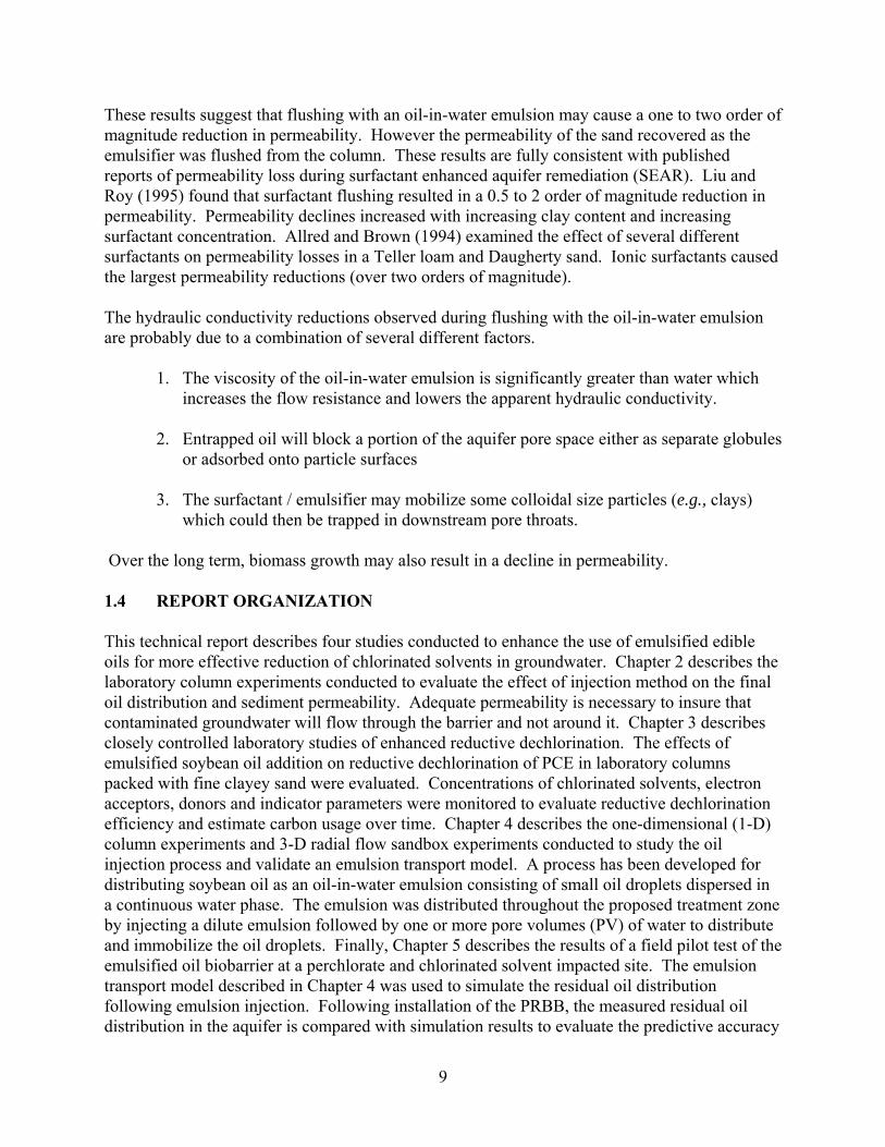
which could then be trapped in downstream pore throats. Over the long term, biomass growth may also result in a decline in permeability. 1.4 REPORT ORGANIZATION This technical report describes four studies conducted to enhance the use of emulsified edible oils for more effective reduction of chlorinated solvents in groundwater. Chapter 2 describes the laboratory column experiments conducted to evaluate the effect of injection method on the final oil distribution and sediment permeability. Adequate permeability is necessary to insure that contaminated groundwater will flow through the barrier and not around it. Chapter 3 describes closely controlled laboratory studies of enhanced reductive dechlorination. The effects of emulsified soybean oil addition on reductive dechlorination of PCE in laboratory columns packed with fine clayey sand were evaluated. Concentrations of chlorinated solvents, electron acceptors, donors and indicator parameters were monitored to evaluate reductive dechlorination efficiency and estimate carbon usage over time. Chapter 4 describes the one-dimensional (1-D) column experiments and 3-D radial flow sandbox experiments conducted to study the oil injection process and validate an emulsion transport model. A process has been developed for distributing soybean oil as an oil-in-water emulsion consisting of small oil droplets dispersed in a continuous water phase. The emulsion was distributed throughout the proposed treatment zone by injecting a dilute emulsion followed by one or more pore volumes (PV) of water to distribute and immobilize the oil droplets. Finally, Chapter 5 describes the results of a field pilot test of the emulsified oil biobarrier at a perchlorate and chlorinated solvent impacted site. The emulsion transport model described in Chapter 4 was used to simulate the residual oil distribution following emulsion injection. Following installation of the PRBB, the measured residual oil distribution in the aquifer is compared with simulation results to evaluate the predictive accuracy

10

of the model. The effects of PRBB installation on groundwater flow, biogeochemical conditions and contaminant concentrations are described. 1.5 REFERENCES Allred B., Brown G. 1994. Surfactant Induced Reductions in Soil Hydraulic Conductivity.

Ground Water Monitoring Review. 174-184. Bagley DM., JM. Gossett. 1989. Tetrachloroethene Transformation to Trichloroethene and cis-1,2-

dichloroethene by Sulfate-reducing Enrichment Culture. Applied & Environmental Microbiology 56(8):2511-16.

Ballapragada BS., HD. Stensel, JA. Puhakka, JF. Ferguson. 1997. Effect of Hydrogen on

Reductive Dechlorination of Chlorinated Ethenes. Environmental Science & Technology 31(6):1728-34.

Bosma TNP., JR. Van der Meer, G.Schraa, ME.Tros, AJB. Zehnder AJB. 1988. Reductive

dechlorination of all trichloro- and dichlorobenzene isomers." FEMS Microbiol. Ecol., 53:223–9.

Bouwer EJ. 1994. Bioremediation of Chlorinated Solvents Using Alternate Electron Acceptors. In

Norris RD, Hinchee RE, Brown R, McCarty PL, Semprini L, Wilson JT, Kampbell DH, Reinhard M, Bouwer EJ, Borden RC, Vogel TM, Thomas JM, Ward CH. Handbook of Bioremediation. pp. 149-75. Boca Raton: Lewis Publishers.

de Bruin WP., MJJ. Kotterman, MA.Posthumus, G. Schraa, AJB. Zehnder. 1992. Complete

Biological Reductive Transformation of Tetrachloroethene to Ethane. Applied & Environmental Microbiology. 58(6):1996-00.

DiStefano TD, JM. Gossett, SH. Zinder. 1991. Reductive Dehalogenation of High Concentrations

of Tetrachloroethene to Ethene by an Anaerobic Enrichment Culture in the Absence of Methanogenesis. Applied & Environmental Microbiology 57(8):2287-92.

Dybas MJ., GM. Tatara, ME.Witt, CS.Criddle. 1997. Slow-release Substrates for

Transformation of Carbon Tetrachloride by Pseudomonas Strain KC. In In Situ and On Site Bioremediation: Vol. 3. Papers from the 4th Int. In Situ and On Site Bioremediation Sym. New Orleans, LA. p. 59. Columbus: Battelle Press.

Fathepure BZ, Boyd SA. 1988. Dependence of Tetrachloroethylene Dechlorination on

Methanogenic Substrate Consumption by Methanoscarnia sp. Strain DCM. Applied & Environmental Microbiology 54(12):2976-2980.

Freedman DL., JM. Gossett. 1989. Biological Reductive Dechlorination of Tetrachloroethylene and

Trichloroethylene to Ethylene Under Methanogenic Conditions. Appl. Environ. Microbiol. 55(9):2144-2151.

11

Gerritse J, Renard V, Pedro-Gomes TM, Lawson PA, Collins MD, et al. 1996. Desulfitobacterium sp. Strain PCE1, an anaerobic bacterium that can grow by reductive dechlorination of tetrachloroethene or ortho-chlorinated phenols. Arch. Microbiol. 165:132-40.

Gibson SA, Suflita JM. 1986. Extrapolation of biodegradation results to groundwater aquifers:

Reductive dehalogenation of aromatic compounds. Appl. Environ. Microbiol. 52:681-688. Gillham RW, O’Hannesin SF, Vogan JL. 1995. Abiotic degradation of chlorinated organic

compounds by zero-valent metals, Written communication to the International Containment Technology Workshop, Permeable Reactive Barriers Session, Baltimore, MD.

Griffith GD, Cole JR, Quensen JF, Tiedje JM. 1992. Specific deuteration of dichlorobenzoate

during reductive dehalogenation by Desulfomonile tiedjei in deuterium oxide. Appl. Environ. Microbiol. 58(1):409-11.

Holliger C. 1995. The anaerobic microbiology and biotreatment of chlorinated ethenes. Current

Opinion in Biotechnol. 6:347-51. Holliger C, Schumacher W. 1994. Reductive dehalogenation as a respiratory process. Antonie van

Leeuwenhoek 66:239-46. Kuhn EP, Suflita JM. 1989. Sequential reductive dehalogenation of chloroanilines by

microorganisms from a methanogenic aquifer. Environ. Sci. Technol., 23:848–52. Lee MD, Quinton GE, Beeman RE, Biehle AA, Liddle RL. 1997. Scale-up issues for in situ

anaerobic tetrachloroethene bioremediation. J. Ind. Microbiol. Biotechnol. 18(2/3):106-15. Lee MD, Buchanan RJ Jr., Ellis DE. 2000. Laboratory studies using edible oils to support

reductive dechlorination, Proc. 2nd Internat. Conf. Remediation of Chlorinated and Recalcitrant Compounds, Battelle Press, Columbus, Ohio.

Liu MW, Roy D. 1995. Surfactant-induced interactions and hydraulic conductivity changes in

soil. Waste Manage. 15: 463-470. Maymo-Gatell X, Chien Y-t, Gossett JM, Zinder SH. 1997. Isolation of a bacterium that

reductively dechlorinates tetrachloroethene to ethene. Sci. 276:1568-71. Neumann A, Scholz-Muramuatsu H, Diekert G. 1994. Tetrachloroethene metabolism of

Dehalospirillum multivorans. Arch. Microbiol. 162:295-01. Quensen JF, Tiedje JM, Boyd SA. 1988. Reductive dechlorination of polychlorinated biphenyls

by anaerobic microorganisms from sediments. Science, 242:752–754. Sanford RA, Cole JR, Loeffler FE, Tiedje JM. 1996. Characterization of Desulfitobacterium

chlororespirans sp. nov., which grows by coupling the oxidation of lactate to the

12

reductive dechlorination of 3-chloro-4-hydroxybenzoate. Appl. Environ. Microbiol. 62(10):3800-08.

Schumacher W, Holliger C. 1996. The proton/electron ratio of the menaquinone-dependent electron transport from dihydrogen to tetrachloroethene in Dehalobacter restrictus. J. Bacteriol. 178(8):2328-33.

Sewell GW, Gibson SA, Russell HH. 1990. Anaerobic in-situ treatment of chlorinated ethenes.

Proc., 1990 Water Pollution Control Federation Annual Conference: In-situ Bioremediation of Groundwater and Contaminated Soil, 68–79.

Sewell GW, Gibson SA. 1991. Stimulation of the reductive dechlorination of tetrachloroethene in

anaerobic aquifer microcosms by the addition of toluene. Environ. Sci. Technol. 25:982-984.

Smatlak C, Gossett JM, Zinder SH. 1996. Comparative kinetics of hydrogen utilization for

reductive dechlorination of tetrachloroethene and methanogenesis in an anaerobic enrichment culture. Environ. Sci. Technol. 30(9):2850-58.

Suflita JM, Sewell GW. 1991. Anaerobic Biotransformation of Contaminants in the Subsurface.

EPA Environmental Research Brief, EPA/600/M-90/024, U.S. Environmental Protection Agency, Ada, Okla.

Utkin I, Woese C, Wiegel J. 1994. Isolation and characterization of Desulfitobacterium

dehalogenans gen. nov., sp. nov., an anaerobic bacterium which reductively dechlorinates chlorophenolic compounds. Int. J. Syst. Bacteriol. 44(4):612-19.

Vogel TM, McCarty PL. 1985. Biotransformation of tetrachloroethylene to trichloroethylene,

dichloroethylene, vinyl chloride, and carbon dioxide under methanogenic conditions. Appl. Environ. Microbiol. 49(5): 1080-83.

Woods SL, Ferguson JF, Benjamin MM. 1988. Characterization of chlorophenol and

chloromethoxybenzene biodegradation during anaerobic treatment. Env. Sci. Tech., 23:62–68.

Zenker, MJ, Borden RC, Barlaz MA, Lieberman MT, Lee MD. 2000. Insoluble electron donors

for reductive dehalogenation in permeable reactive barriers, Proc. 2nd Internat. Conf. Remediation of Chlorinated and Recalcitrant Compounds, Battelle Press, Columbus, Ohio.

13

INJECTION OF NEAT AND EMULSIFIED EDIBLE OILS - RESIDUALSATURATION AND PERMEABLITY IMPACTS 2.1 INTRODUCTION Enhanced anaerobic bioremediation can be a cost-effective approach for treating a variety of groundwater contaminants including certain heavy metals, nitrate, perchlorate, acid mine drainage and chlorinated organics. Many highly chlorinated organics are resistant to aerobic biodegradation but are degradable under anaerobic conditions through a process termed reductive dehalogenation where the chlorinated organic compound serves as an electron acceptor and the chloride moiety is removed and replaced by hydrogen, forming a less chlorinated and more reduced intermediate (Sewell et al., 1990). This process has been demonstrated for a wide range of chlorinated organics including tetrachloroethene (PCE), trichloroethene (TCE), cis- and trans-1,2-dichloroethene (cis-DCE and trans-DCE) and vinyl chloride (VC) (Sewell and Gibson, 1991; Freedman and Gossett, 1989; de Bruin et al., 1992). A wide variety of substrates can be used as electron donors for reductive dehalogenation including acetate, butyrate, benzoate, glucose, lactate, methanol, toluene and hydrogen (Lee et al., 1998). The most common approach for stimulating in-situ anaerobic biodegradation of contaminated groundwater has been to circulate water containing a dissolved, readily biodegradable organic substrate through the treatment zone. This approach has been very effective at some sites (Ellis et al., 2000; Martin et al., 2001; Major et al., 2002). However problems with clogging of process piping, injection and pumping wells may increase operation and maintenance costs. An alternative approach employed at some sites has been to distribute a ‘slow-release’ organic substrate throughout the treatment zone that can support anaerobic biodegradation of the target contaminants for an extended time period. Slow-release substrates used include cellulose, chitin, Hydrogen Release Compound (HRC®) and certain edible oils. HRC is a polymerized ester that dissolves over time releasing lactate which can support anaerobic biodegradation of chlorinated solvents and other contaminants (Koenigsberg et al., 2000; Wu 1999). A variety of edible fats and oils have been shown to support reductive dehalogenation including corn oil, hydrogenated cottonseed oil beads, and solid food shortening (Dybas et al., 1997), beef tallow, melted corn oil margarine, and coconut oil (Lee et al., 1998). Zenker et al. (2000) screened a variety of organic substrates to identify materials that would slowly biodegrade over time. Subsequent studies showed that both liquid soybean oil and semi-solid hydrogenated soybean oil could support complete dehalogenation of TCE to ethene in microcosms containing sediment from a chlorinated solvent impacted site. Studies by Hunter (2001; 2002) demonstrated that soybean oil could be used to stimulate anaerobic degradation of other problem contaminants including nitrate and perchlorate. One common method for use of edible oils has been the installation of biologically active permeable reactive barriers. In this approach, edible oils are injected through a series of temporary or permanent wells installed perpendicular to groundwater flow. As groundwater moves through the oil treated zone under the natural hydraulic gradient, a portion of the oil dissolves providing a carbon and energy source to accelerate the anaerobic biodegradation processes. Two different approaches have been used to distribute the oil: (1) injection of pure

14

liquid oil (neat oil) (Boulicault et al., 2000); and (2) injection of an oil-in-water emulsion followed by a water flush to distribute emulsion throughout the treatment zone (Borden et al., 2001; Lee et al., 2001). In this chapter, laboratory column experiments were conducted to evaluate the effect of injection method on the final oil distribution and sediment permeability. Permeability loss is a critical parameter in the design of an edible oil barrier. If permeability loss is excessive, contaminated groundwater will flow around the barrier and will not be treated. 2.2 MATERIALS AND METHODS 2.2.1 Injection Procedure Injections tests were conducted on sediments with varying grain size distributions and clay contents (Table 2.1). The field sand and concrete sand used in this project were purchased from local suppliers (Raleigh, NC). Ottawa ASTM 20/30 sand was purchased from U.S. Silica Company (Ottawa, Illinois). Kaolinite (Thiele Kaolin Company, Sandersville, Georgia) was added to certain materials to evaluate the effect of increasing clay content. Grain size distributions for each material are presented in Figure 2.1. All materials tested are classified as sands (D50 > 0.3mm) with less than 15% passing a #200 sieve (Table 2.1). The pore size distribution of each material (Figure 2.2) was calculated from the grain size distribution using the procedure presented by Barr (2001) with 20 separate size increments (Arya et al., 1999).

Table 2.1 Characteristics of Sediments used in Permeameter Studies

Material D50 (mm)

D10 (mm)

Cu D60 / D10

% Finer than 75 μm (#200 sieve)

Hydraulic Conductivity

(cm/s)

Ottawa Sand 1.07 0.66 1.9 1.2 0.41 ± 0.06

Play Sand 0.30 0.10 3.3 1.1 0.024 ±0.004

Concrete Sand + 5% clay 0.74 0.03 34.8 14.7 0.041 ± 0.013

Concrete Sand 0.82 0.15 8.2 9.0 0.053 ±0.027

Field Sand 0.38 0.1 4.5 6.9 0.011 ± 0.003

Field Sand + 3% clay 0.37 0.07 6.7 10.5 0.006 ± 0.001

Hydraulic conductivity values are mean ± 1 standard deviation of replicate measurements.

15

0

10

20

30

40

50

60

70

80

90

100

0.001 0.01 0.1 1 10Grain Size (mm)

Cum

ulat

ive

Wei

ght (

%)

Concrete sand + 5% clayOttawa sandPlay sandField sandField sand + 3% clayConcrete sand

Figure 2.1 Grain size distribution of each material.

0

0.1

0.2

0.3

0.4

0.5

0.6

0.7

0.8

0.9

1

0.001 0.01 0.1 1

Pore Diam eter (mm )

Cum

ulat

ive

Volu

me

(%) Concrete sand

Field sand + 3% clayField sandPlay sandConcrete sand + 5% clay

Figure 2.2 Cumulative pore diameter distribution of each material calculated using Barr

(2001) procedure and grain size distributions from Fig 1. The effect of oil injection on sediment permeability was measured in 11.4 cm diameter x 21.1 cm long columns (ASTM D2434 sand and gravel permeameter from ELE, Melbourne, Florida) with influent supplied by a peristaltic pump (Cole-Palmer Masterflex). Head loss was measured with wall mounted manometer tubes and the outflow recorded over time using a stopwatch. The columns were packed with dry sediment in 3 to 5 cm lifts. After each lift, the sediment was

16

repeatedly compacted with a 5 cm rubber stopper mounted on a metal rod to achieve a density of approximately 1.8 g/cm3. After packing, a vacuum was applied to the column and it was slowly flooded to minimize entrapped air. Deaired tap water was then pumped through the column until the permeability stabilized (0.5 to 2 hours depending on the sediment) and then the hydraulic conductivity (K) was measured at least twice over a 10-25 min period. Neat soybean oil injection was evaluated by pumping ~2.4 L of liquid soybean oil (~ 4 pore volumes) through each sediment followed by deaired tap water until the permeability stabilized (minimum of 20 pore volumes (PV)). All materials were tested in triplicate. Changes in head loss in the manometer tubes were monitored with time to evaluate the change in effective permeability of the sediment as oil is injected and then displaced with water. The final oil residual saturation is determined by volatile solids (VS) analysis of three ~2.5 cm diameter by 13 cm long sediment cores. Sediment moisture content is determined by weight loss after drying at 105 ºC for 24 hours (48 hours for liquid samples). VS are determined by weight loss on ignition for 1 hour at 550 ºC. Emulsion injection was evaluated following the same general procedures used for neat oil injection. A minimum of 3 PV of emulsion were injected followed by 6 to 10 PV of water (enough to reach residual saturation). At the end of each PV, an effluent sample was collected and the permeability was measured. The sediment moisture content and final oil retention was determined by VS analysis. 2.2.2. Emulsion Preparation

The food preparation industry has tremendous experience in producing stable oil-in-water emulsions with a uniformly small droplet size. The key factors in generating the desired emulsion are: (1) the oil-water interfacial tension; and (2) the mixing energy. Small droplets can be generated using surfactants that result in a low interfacial tension (less than 1 dyne/cm). However, these emulsions may be unstable and the small droplets may coalesce forming larger droplets with time. The most stable emulsions are often produced at moderate interfacial tensions (5 – 10 dyne/cm) with very high mixing energy. Using this information, a series of studies were conducted to identify combinations of surfactants and mixers that generate stable oil-in-water emulsions with a small, uniform droplet size distribution. The droplet size distribution was measured visually with a Nikon™ microscope equipped with a Sensys™ calibrated camera and Metamorph™ software at a 400x magnification. A series of food grade surfactants were first screened to identify those with desirable properties. Air-water and oil-water interfacial tension was measured with a surface tensiometer equipped with a platinum iridium ring (Fisher Scientific). Once several potential surfactants were identified, emulsification studies were conducted to evaluate the effect of mixing energy on the resulting oil droplet size distribution. Coarse emulsions were first prepared using a fixed ratio of oil to surfactant to water in a kitchen blender. These emulsions were then subjected to progressively higher levels of mixing energy.

17

Nine different food-grade emulsifiers were initially screened for their ability to generate stable soybean oil-in-water emulsions. A mixture of 160 ml tap water, 40 ml oil and 2, 4 or 6 g of each emulsifier were manually shaken for three minutes and then stored for 24 hours. The emulsifiers that were easiest to blend with water and yielded a stable emulsion were considered the best. Based on this initial screening, lecithin with hydrophilic/lipophilic balance (HLB) of 4 (Centrophase C from Central Soya), polysorbate 20, polysorbate 21, polysorbate 85 (from UNIQUEMA) and a surfactant mixture (38% polysorbate 80, 56% glycerol monooleate (GMO) and 6% water from Lambent Technologies) were selected for further evaluation. The soybean oil-water interfacial tension of 2% solutions of surfactant in water were as follows: 28 dyne/cm for no surfactant, 8 dyne/cm for polysorbate 20, 8.3 dyne/cm for polysorbate 21, 9.7 dyne/cm for polysorbate 85 and 11 dyne/cm for the polysorbate 80-GMO mixture. The interfacial tension of the lecithin could not be measured because the low HLB prevented it from dissolving in water. A series of tests were then conducted to evaluate the effect of different surfactants and mixers on the resulting droplet size distribution. The following mixing procedures were evaluated: (1) mixing at high speed in a standard kitchen blender (Westinghouse) for 5 minutes; (2) mixing for 5 minutes using a hand-held homogenizer at the highest setting (Ultra Turrax RKA T18, Fisher Scientific); (3) mixing for 5 minutes using a lab sonicator (Sonic Dismembrator Model 550, Fisher Scientific); (4) repeated passage through a Silverson high shear laboratory mixer (LART-W) with the EMSC-F mixing heads; (5) one pass through a commercial dairy homogenizer (Gaulins two stage 300 GCI) at 1000 psi; (6) mixing for 3 minutes at low speed in a 1 gallon Waring Commercial Blender; and (7) mixing for 5 minutes at high speed in the same blender. Photomicrographs of several of the emulsions are shown in Figure 2.3.

Figure 2.3 Emulsion droplets produced with different surfactants and mixing devices as described in Table 2.3. White scale bar is 25 µm.

#4 - Kitchen Blender #6 - Lab Sonicator

#2 - High Shear Mixer3 passes

#3 - High Shear Mixer >10 passes

#9 - Gaulins Homogenizer

18

Most of the oil droplet size distributions are strongly non-symmetric with many small droplets and a few large droplets. However the few large droplets contain a substantial portion of the total oil since the droplet volume is proportional to the diameter cubed. To provide a more useful presentation of these results, a statistical summary of the Log10 transformed droplet size distribution is presented in Table 2.2. The cumulative oil volume vs. droplet diameter for the different mixers is presented in Figure 2.4.

Table 2.2 Characteristics of Droplet Size Distributions from Different Surfactant –

Mixer Combinations. Statistics are for Log10 Transformed Distribution of the Oil Droplet Diameter.

# Surfactant Mixer Mixing

time Median

(μm) Mean (μm)

Standard Deviation

(μm)

Skewness of

Log Diameter

1 Centrophase C lecithin

Kitchen blender on high speed 5 min. 2.7 3.9 3.1 0.7


Silverson high shear mixer 3 passes 2.4 3.0 2.2 1.2


Silverson high shear mixer

10 passes 3.2 3.6 1.5 0.5

4 Polysorbate 85 Kitchen blender on high speed 5 min. 4.6 4.8 1.7 0.4

5 Polysorbate 85 Lab. Homogenizer 5 min. 3.2 3.4 1.7 0.7

6 Polysorbate 85 Lab. Sonicator 5 min. 1.4 1.5 1.6 0.6

7 Polysorbate 80-GMO Waring blender on low speed 3 min. 7.4 7.2 1.6 -0.3

8 Polysorbate 80-GMO Waring blender on high speed 5 min. 1.2 1.2 1.3 0.2

9 Polysorbate 80-GMO Gaulins homogenizer 1 pass 0.7 0.7 1.3 -0.3

19

0102030405060708090

100

0 10 20 30Droplet Size (um)

Cum

ulat

ive

Volu

me

(%)

#9

#8

#6

#3

#5

#7

#4

#2

#1

Figure 2.4 Cumulative droplet volume distributions for different emulsion preparation methods. Emulsion numbers and preparation methods are listed in Table 2.2.

The modified lecithin (Centrophase C) resulted in coarse emulsion with a large average droplet size and wide range of droplets. In contrast, both the polysorbate 85 and polysorbate 80 - GMO mixture generated droplet size distributions with smaller, more uniform droplets. A single pass through the Silverson mixer generated a very coarse emulsion that separated rapidly (data not shown). However over 10 passes through the Silverson laboratory mixer (equivalent to > 4 passes through a full-size mixer) generated a good emulsion that was stable with small, uniform droplets. The Gaulins homogenizer and the Waring commercial blender at high speed for 5 minutes provided the smallest, most uniform droplets. Emulsions prepared with polysorbate 80 - GMO and both the Silverson high shear mixer and dairy homogenizer were stable for at least one month when stored at 4 oC. Droplet size distributions from both mixers were measured immediately after preparation, after storage for one week and after storage for one month. For both mixers, there was no significant change in the droplet size distribution (data not shown). The median droplet size of all emulsions generated in this study were significantly smaller than the median pore size of all the sediments suggesting that most droplets could be easily transported through the different sands. However, some of the emulsions have a highly variable droplet size distribution with a few very large (> 50 µm) droplets. In these emulsions, much of the oil is present in largest droplets which could be rapidly removed by straining.

20

2.3 NEAT OIL INJECTION RESULTS The laboratory column tests demonstrated that neat soybean oil can be distributed in sands with little or no clay. However with the equipment available in our laboratory, it was not practical to inject soybean oil in sediments with any significant clay content. For the three sands tested, oil residual saturation after flushing with over 30 PV of water varied from 22 to 54% (Table 2.3). Residual saturation was lowest in the most uniform material (Ottawa sand) and highest in the more broadly graded concrete sand. This is consistent with the results of Chatzis and Morrow (1984) who observed that a broader grain size range leads to a higher residual saturation. For the three sands tested, the final permeability after over 30 PV of water displacement was just below half of the initial permeability, indicating that if the oil could be displaced to residual saturation, the permeability loss would not be excessive.

Table 2.3 Residual Saturation and Change in Hydraulic Conductivity Following

Injection with Neat Soybean Oil.

Media

Oil Residual Saturation (% by volume of pore space)

Initial Hydraulic Conductivity (Ko) (cm/s)

Final Hydraulic Conductivity (K) (cm/s)

K/Ko

Ottawa Sand 21.7 (3.7) 0.427 (0.035) 0.185 (0.057) 46(12)

Concrete Sand 54.2 (7.9) 0.051 (0.002) 0.026 (0.007) 45 (0)

Play Sand 36.5 (2.5) 0.027 (0.006) 0.011 (0.001) 46 (18)

Concrete Sand + 5% kaolinite 31.0 (0.1) 0.019 (0.004) 0.008 (0.003) 39 (14)

a Residual saturation and permeability change are the average of triplicate column tests. Standard deviations are shown in parentheses.

However, a number of operational problems were identified during oil injection that would complicate application of neat oil injection in the field. At typical groundwater temperatures (10 to 20 ºC), soybean oil has a viscosity 60 to 70 times that of water which makes it very difficult to move neat oil any significant distance from the injection point. Figure 2.5 shows the hydraulic gradient (m of water head/m) required to pump 2 PV of water, 3 PV of liquid soybean oil and then 7 PV of water through Ottawa sand at a constant flow rate. There is an almost two order of magnitude increase in the hydraulic gradient during soybean oil injection. Once the oil is displaced to residual saturation, hydraulic conductivity returns to roughly half of the pre-injection value. However, 20 to 30 PV of water flushing is required to achieve this. In the field, extended flushing with water to reach residual saturation would not be practical. However if the soybean oil is not displaced to residual saturation, it will float upward due to its lower density. Finally, the high residual saturation of soybean oil in sand would require injection of large volumes of oil. High pressure buildup, injection of large volumes of oil and high water flush

21

after oil injection could hinder cost effectiveness of the use of soybean oil as a substrate for enhanced reductive dechlorination if neat oil is to be injected. The next step to make this technology viable is to implement alternative techniques to inject soybean oil in the subsurface while avoiding or minimizing the aforementioned problems.

0.1

1

10

100

-2 0 2 4 6 8 10Pore Volumes

Hyd

raul

ic G

radi

ent

(cm

/cm

)

Oil Water

Figure 2.5 Variation in hydraulic gradient during injection of Ottawa sand with 3 pore

volumes of neat soybean oil followed by plain water at constant flow rate.

Therefore, the remainder of this chapter focuses on the development of methods for distributing soybean oil-in-water emulsions in representative aquifer materials, which appears as a promising way of injecting soybean oil without significant adverse side effects. 2.4 EMULSION INJECTION RESULTS The most commonly adopted model for emulsion transport in porous media was proposed by Soo and Radke (1984) to describe emulsion transport and associated clogging in petroleum reservoirs. These investigators conducted a series of experiments examining the transport of emulsions with different droplet size distributions through fine Ottawa sand cores (intrinsic permeability = 1.5 µm2 and 0.57 µm2). The emulsions used by Soo and Radke were prepared with refined mineral oil (Chevron 410H) stabilized with sodium oleate and oleic acid, mixed with sodium hydroxide to minimize droplet sticking to the surface of sediment particles and also minimize droplet coalescence. Results of these experiments demonstrated that oil droplets smaller than the sediment pores could be transported significant distances through porous media with low interception by solid surfaces and low permeability loss to the porous media. However, injection of oil droplets larger than the sediment pores resulted in rapid droplet removal by straining with a large, permanent permeability loss. Our objective was to develop a method for distributing oil-in-water emulsions significant distances away from the injection point with low to moderate permeability loss and moderate oil retention. Preliminary calculations indicate that depending on environmental conditions, a 3 m wide barrier with 0.5 to 2 % residual oil should contain enough organic material to support anaerobic biodegradation for 10 years or more. Excessive permeability loss could cause contaminated groundwater to flow around the emulsion impacted zone and not be treated. High oil retention could increase the amount of oil required above that necessary for treatment of the

22

contaminants. However too low an oil retention could allow the oil droplets to migrate out of the target treatment zone requiring more frequent injection and possibly impacting downgradient receptors. The sediments examined in this study had median pore sizes (D50) between 35 and 125 µm with some pores less than 10 µm (Figure 2.2). Adding clay to the concrete and field sands significantly reduced the estimated D50 of the pores indicating that sediments with higher clay contents will require emulsions with smaller droplet size distributions. In addition, the added clay may increase interception since the small oil droplets may be more likely to stick to the charged clay surfaces. Based on the work of Soo and Radke (1986a; 1986b), we concluded that an emulsion was needed with small (less than 10 µm), uniformly sized droplets. Ideally, the sediment-droplet collision efficiency should be low to moderate allowing the oil droplets to be transported some distance before they are immobilized on the sediment surfaces. 2.4.1 Emulsion Transport and Permeability Loss Column experiments were conducted to evaluate emulsion transport and associated permeability loss in concrete sand, field sand and field sand +3% added clay (kaolinite) with both coarse and fine emulsions. The cumulative oil volume vs. droplet diameter for the coarse and fine emulsions is shown in Figure 2.4 as emulsions 7 and 8. The variation in emulsion concentration in the column effluent and effective hydraulic conductivity of field sand treated with fine emulsion is shown in Figure 2.6. The emulsion concentration is presented as the measured VS concentration of the column effluent divided by the VS of the injected emulsion (C/Co). K is calculated as the observed hydraulic gradient divided by the flowrate per unit area. During injection, the emulsion rapidly breaks through in the column effluent with little evidence of retardation. Then during the post-injection water flush, the emulsion rapidly declines to background levels with little evidence of tailing or flushout of trapped emulsion. The effective K declines to ~ 66% of the preinjection value and then returns to background levels during the water flushing. Most of the observed reduction in K is due to the higher viscosity of the emulsion (1.44 centipoise) compared to water (0.95 centipoise) at the ambient temperature (23 ºC).

23

00.20.40.60.8

1


C/C

oEmulsion

Water

02468

10


Hydr

aulic

Co

nduc

tivity

(m/d

)

Figure 2.6 Variation in emulsion concentration (C/Co) in column effluent and effective hydraulic

conductivity during injection of field sand with 3 pore volumes of fine emulsion followed by plain water.

Figure 2.7 shows the effective K when concrete sand, field sand and field sand + 3% clay are treated with coarse or fine emulsion. For each material, the initial K of the material can vary by 30% or more due to minor differences in packing of the columns. The effective K of the concrete sand dropped by 40-44% during injection of the coarse emulsion and then rebounded during water flushing resulting in a final permeability loss of 12-19%. The small K reduction and low oil retention (Table 2.4) is due to the large ratio of pore size to droplet size.

24

Concrete Sand

05

101520253035404550

-2 0 2 4 6 8 10 12

Pore Volumes

K (m

/d)

Coarse-1Coarse-2

Emulsion Water

Field Sand

0

2

4

6

8

10

12

14

16

18

-2 0 2 4 6 8 10 12

Pore Volumes

K (m

/d)

Coarse-1 Coarse-2Coarse-3Fine-1 Fine-2

EmulsionWater

Field Sand + 3% Clay

0

1

2

3

4

5

6

7

8

9

10

-2 0 2 4 6 8 10 12

Pore Volumes

K (m

/d)

Coarse-1 Coarse-2Coarse-3Fine-1 Fine-2

EmulsionWater

Figure 2.7 Variation in K during injection of concrete sand, field sand and field sand + 3% clay with

three volumes of either coarse or fine emulsion followed by water flushing.

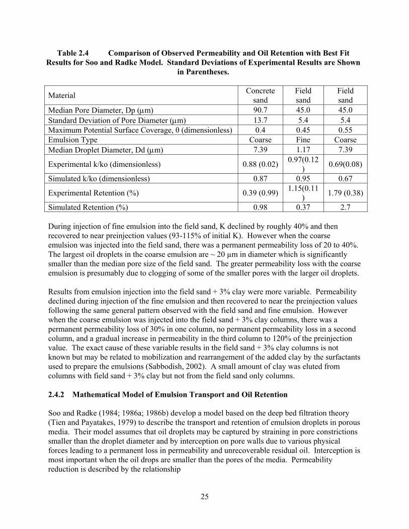
25

Table 2.4 Comparison of Observed Permeability and Oil Retention with Best Fit Results for Soo and Radke Model. Standard Deviations of Experimental Results are Shown

in Parentheses.

Material Concrete sand

Field sand

Field sand

Median Pore Diameter, Dp (μm) 90.7 45.0 45.0 Standard Deviation of Pore Diameter (μm) 13.7 5.4 5.4 Maximum Potential Surface Coverage, θ (dimensionless) 0.4 0.45 0.55 Emulsion Type Coarse Fine Coarse Median Droplet Diameter, Dd (μm) 7.39 1.17 7.39

Experimental k/ko (dimensionless) 0.88 (0.02) 0.97(0.12) 0.69(0.08)

Simulated k/ko (dimensionless) 0.87 0.95 0.67

Experimental Retention (%) 0.39 (0.99) 1.15(0.11) 1.79 (0.38)

Simulated Retention (%) 0.98 0.37 2.7 During injection of fine emulsion into the field sand, K declined by roughly 40% and then recovered to near preinjection values (93-115% of initial K). However when the coarse emulsion was injected into the field sand, there was a permanent permeability loss of 20 to 40%. The largest oil droplets in the coarse emulsion are ~ 20 µm in diameter which is significantly smaller than the median pore size of the field sand. The greater permeability loss with the coarse emulsion is presumably due to clogging of some of the smaller pores with the larger oil droplets. Results from emulsion injection into the field sand + 3% clay were more variable. Permeability declined during injection of the fine emulsion and then recovered to near the preinjection values following the same general pattern observed with the field sand and fine emulsion. However when the coarse emulsion was injected into the field sand + 3% clay columns, there was a permanent permeability loss of 30% in one column, no permanent permeability loss in a second column, and a gradual increase in permeability in the third column to 120% of the preinjection value. The exact cause of these variable results in the field sand + 3% clay columns is not known but may be related to mobilization and rearrangement of the added clay by the surfactants used to prepare the emulsions (Sabbodish, 2002). A small amount of clay was eluted from columns with field sand + 3% clay but not from the field sand only columns. 2.4.2 Mathematical Model of Emulsion Transport and Oil Retention Soo and Radke (1984; 1986a; 1986b) develop a model based on the deep bed filtration theory (Tien and Payatakes, 1979) to describe the transport and retention of emulsion droplets in porous media. Their model assumes that oil droplets may be captured by straining in pore constrictions smaller than the droplet diameter and by interception on pore walls due to various physical forces leading to a permanent loss in permeability and unrecoverable residual oil. Interception is most important when the oil drops are smaller than the pores of the media. Permeability reduction is described by the relationship

26

k/k0 = 1- βσ/ε0

where β is the flow restriction parameter, σ is the oil retention and ε0 is the initial porosity. Intrinsic permeability (k) is calculated as k = Kρ/µ where K is the effective hydraulic conductivity, ρ is the density of the injection fluid, and µ is the viscosity of the injection fluid. The model does not explicitly consider the various electrostatic forces that may influence droplet interception. However it does include a surface coverage parameter (θ) that varies between 0 – 1 and represents the fraction of pore wall surface that can be covered by the droplets. The model input parameters with the greatest impact on simulated permeability loss are the average pore size of the sediment, median pore diameter (dp), median droplet diameter (dd), the standard deviation of the pore size distribution, and θ. There is no method for independently estimating θ, so this parameter was used as a fitting parameter to achieve the best fit between simulated and observed k/ko. The model was coded in visual basic for application in a spreadsheet, then θ is varied manually to match the observed values. Model parameters are presented in Table 2.4. Figure 2.8 shows the simulated and observed changes in intrinsic permeability during injection of the concrete sand and field sand with 3 PV of coarse or fine emulsion followed by 7 PV of plain water. All of the experimental curves show the same general trend with an initial drop in k/ko during emulsion injection followed by no significant change in k/ko during water flushing. There is no recovery in k/ko during water flushing since plotting intrinsic permeability automatically accounts for differences in the viscosity and density of the water and emulsion. The Soo and Radke model reproduces the experimental reduction in k/ko very well. However this model was not nearly as accurate in simulating oil retention (Table 2.4). The match between simulated and observed oil retention could be improved by increasing θ. However the required increases in θ are not physically realistic and would result in excessively high simulated k losses. A major limitation of the Soo and Radke model is the assumption of a perfectly uniform droplet size distribution. However in practice, emulsions have a range of droplet sizes with most of the oil present in a few large droplets. For the coarse emulsion, over 85% of the total oil volume was present in oil droplets greater than the median droplet diameter (7.5 µm).

27

0.4

0.5

0.6

0.7

0.8

0.9

1

0 2 4 6 8 10 12Pore Volume

k/k o

Field sand - Coarse emulsionField sand - Fine emulsionConcrete Sand - Coarse emulsionSoo and Radke

Figure 2.8 Comparison of Soo and Radke model with observed variation in relative permeability when concrete sand and field sand are flushed with 3 PV of coarse or fine emulsion followed by plain water. Error bars show the range of experimental measurements in triplicate columns.

2.4.3 Effect of Clay Content on Emulsion Residual Saturation and Permeability Loss Figure 2.9 shows the variation in oil residual saturation (oil content after emulsion injection followed by over 8 PV of water flushing) with clay content and includes results using a variety of different emulsion preparation methods (lecithin and polysorbate - GMO with both coarse and fine emulsions). Oil retention increases linearly with sediment clay content (r2= 0.81, p<0.0001). This is not unexpected since when oil droplets are smaller than the sediment pores, straining losses are low and oil capture should be dominated by interception. The large surface area and negative charge associated with the clay particles may significantly enhance oil droplet interception.

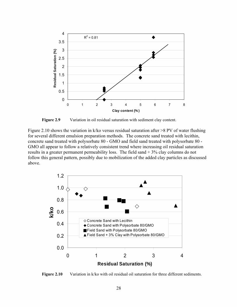
28

R2 = 0.81

0

0.5

1

1.5

2

2.5

3

3.5

4

0 1 2 3 4 5 6 7 8

Clay content (% )

Res

idua

l Sat

urat

ion

(%)

Figure 2.9 Variation in oil residual saturation with sediment clay content.

Figure 2.10 shows the variation in k/ko versus residual saturation after >8 PV of water flushing for several different emulsion preparation methods. The concrete sand treated with lecithin, concrete sand treated with polysorbate 80 - GMO and field sand treated with polysorbate 80 - GMO all appear to follow a relatively consistent trend where increasing oil residual saturation results in a greater permanent permeability loss. The field sand + 3% clay columns do not follow this general pattern, possibly due to mobilization of the added clay particles as discussed above.

0.0

0.2

0.4

0.6

0.8

1.0

1.2

0 1 2 3 4Residual Saturation (%)

k/ko

Concrete Sand with LecithinConcrete Sand with Polysorbate 80/GMOField Sand with Polysorbate 80/GMOField Sand + 3% Clay with Polysorbate 80/GMO

Figure 2.10 Variation in k/ko with oil residual oil saturation for three different sediments.

29

2.4.4 Modeling Permeability Loss from Residual Oil A number of different relationships have been proposed to describe the permeability loss resulting from entrapped particles (bacteria, clay and other colloids). One of the first relationships was proposed by Ives and Pienvichitr (1965) for describing permeability reduction due to biofilm growth where

k/ko=(1-α) 3-P

and α is the fraction of the total pore space occupied by entrapped particles (particle volume/pore volume) and P a parameter to account for tortuous pores. Tien (1989) observed that the Pienvichitr relationship consistently under-predicted permeability loss and proposed the relationship

k/ko=(1-α)3(1+ηo*α/(1-ηo))-4/3

where ηo is the initial porosity. Renshaw et al (1997) introduced a different approach where retained particles are considered as an equivalent clay fraction and

kfinal=ko(1-νclay) kclay

νclay

where kclay is the permeability of the retained clay and νclay is the volume fraction of clay. Figure 2.11 shows a comparison of computed versus observed permeability loss in the field sand and concrete sand for both the Tien and Renshaw relationships. νclay was computed from the oil residual saturation and bulk density of the porous media and oil. There was no way to predict the effective permeability of pure entrapped oil so kclay was used as a fitting parameter. Tien’s model significantly underestimates the permeability loss. The Renshaw model was fitted successfully to the experimental data (Root Mean Square Error=0.072 vs 0.188 for Tien, 1989) and may be appropriate for simulating permeability loss in field-scale edible oil barriers. The best fit for the Renshaw model was obtained with a kclay value of 5.64 x 10-27 cm/s (5.64 x 10-24 darcys) which implies that the trapped oil droplets are essentially impermeable to water.

30

0.4

0.5

0.6

0.7

0.8

0.9

1

0.4 0.5 0.6 0.7 0.8 0.9 1

Measured k/ko

Com

pute

d k/

ko

Tien (1989)

Renshaw et al. (1997)

Figure 2.11 Comparison of measured and computed values of k/ko for Tien (1989) and

Renshaw et al. (1997) models. 2.5 DISCUSSION Our experimental results demonstrate that neat soybean oil can be distributed short distances in sands without excessive permeability loss if the oil can be displaced to residual saturation. However in the field, oil displacement to residual saturation may be very difficult because of the high viscosity of the soybean oil and the large volumes of injection water required. If the oil is not displaced to residual saturation, permeability losses will be significantly higher and there is potential for upward migration of the oil due to buoyancy effects. Injection of soybean oil as an oil-in-water emulsion appears to offer many advantages over injection of neat oil. Soybean oil-in-water emulsions can be prepared using only food-grade, Generally Recognized As Safe (GRAS) materials to aid in gaining regulatory approval. Using appropriate combinations of surfactants and high-energy mixers, emulsions with very small droplets can be prepared that will easily pass through the pores of most sandy sediments. For the fine emulsions used in this study, the primary mechanism of oil retention is believed to be interception, where oil droplets collide with pore surfaces and stick. Retention of these emulsions is very low in pure sand and increases linearly with clay content. Emulsion injection into aquifer material does result in some permeability loss. However for sands with low to moderate clay content, the permeability loss is modest (0 to 40% loss) and is proportional to the oil residual saturation. The low permeability loss observed in our work appears to contradict results by Jain and Demond (2002) who observed large permeability losses when columns packed with pure silica sand were flushed with emulsions prepared with Perchloroethylene (PCE) and either Witconol 2722 or Witconol SN 120 (FDA approved surfactants used to mobilize PCE). The difference in results observed by Jain and Demond and our own results is likely due to the surface characteristics of the emulsions and sediments. In the work by Jain and Demond, the zeta

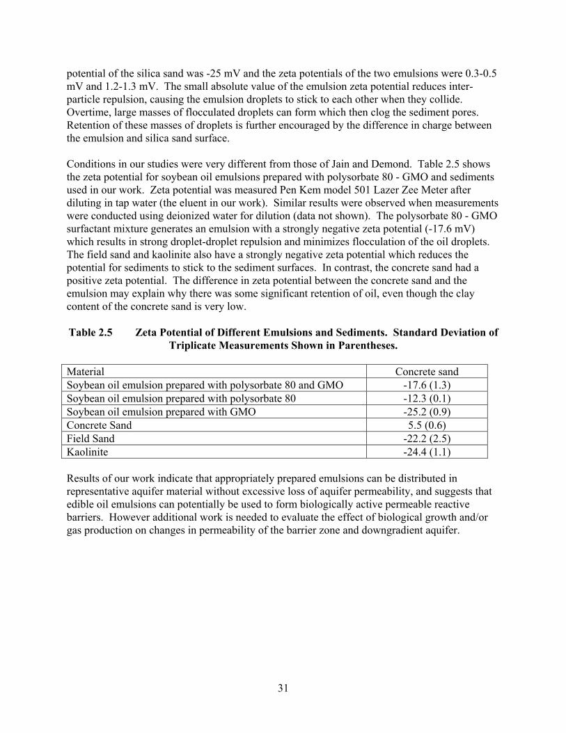
31

potential of the silica sand was -25 mV and the zeta potentials of the two emulsions were 0.3-0.5 mV and 1.2-1.3 mV. The small absolute value of the emulsion zeta potential reduces inter-particle repulsion, causing the emulsion droplets to stick to each other when they collide. Overtime, large masses of flocculated droplets can form which then clog the sediment pores. Retention of these masses of droplets is further encouraged by the difference in charge between the emulsion and silica sand surface. Conditions in our studies were very different from those of Jain and Demond. Table 2.5 shows the zeta potential for soybean oil emulsions prepared with polysorbate 80 - GMO and sediments used in our work. Zeta potential was measured Pen Kem model 501 Lazer Zee Meter after diluting in tap water (the eluent in our work). Similar results were observed when measurements were conducted using deionized water for dilution (data not shown). The polysorbate 80 - GMO surfactant mixture generates an emulsion with a strongly negative zeta potential (-17.6 mV) which results in strong droplet-droplet repulsion and minimizes flocculation of the oil droplets. The field sand and kaolinite also have a strongly negative zeta potential which reduces the potential for sediments to stick to the sediment surfaces. In contrast, the concrete sand had a positive zeta potential. The difference in zeta potential between the concrete sand and the emulsion may explain why there was some significant retention of oil, even though the clay content of the concrete sand is very low.

Table 2.5 Zeta Potential of Different Emulsions and Sediments. Standard Deviation of

Triplicate Measurements Shown in Parentheses.

Material Concrete sand Soybean oil emulsion prepared with polysorbate 80 and GMO -17.6 (1.3) Soybean oil emulsion prepared with polysorbate 80 -12.3 (0.1) Soybean oil emulsion prepared with GMO -25.2 (0.9) Concrete Sand 5.5 (0.6) Field Sand -22.2 (2.5) Kaolinite -24.4 (1.1) Results of our work indicate that appropriately prepared emulsions can be distributed in representative aquifer material without excessive loss of aquifer permeability, and suggests that edible oil emulsions can potentially be used to form biologically active permeable reactive barriers. However additional work is needed to evaluate the effect of biological growth and/or gas production on changes in permeability of the barrier zone and downgradient aquifer.

32

2.6 REFERENCES Arya, L.M., Leij, F.J., Shouse, P.J., Van Genuchten, M.Th., 1999. Relationship between the

hydraulic conductivity function and the particle-size distribution. Soil Sci. Soc. Am. J., 63, 1063-1070.

Barr, D.W., 2001. Coefficient of permeability determined by measurable parameters. Ground

Water, 39, 356-361. Borden, R.C., Coulibaly, K.M., Long, C.M., and, Harvin A.S., 2001. Development of permeable

reactive barriers (PRBs) using edible oils, Annual Report to the Strategic Environmental Research and Development Program.

Boulicault, K.J., Hinchee, R.E., Wiedemeier, T.H., Hoxworth, S.W., Swingle, T.P., Carver, E.,

Haas, P.E., 2000. Vegoil: A Novel Approach for Stimulating Reductive Dechlorination. In: Wickramanayake, G.B., Gavaskar, A.R., Alleman, B.C., Magar, V.S. (Eds) Bioremediation and Phytoremediation of Chlorinated and Recalcitrant Compounds, Battelle Press. pp. 1-7.

Chatzis, I., Morrow N.R., 1984. Correlation of capillary number relationships for sandstones.

Society Petro. Engr. J. 24, 555-562. De Bruin, W.P., Kotterman, M.J.J., Posthumus, M.A., Schraa, G., Zehnder, A.J.B., 1992. Complete

biological reductive transformation of tetrachloroethene to ethane. Appl. Environ. Microbiol. 58, 1996-2000.

Dybas, M.J., Tatara, G.M., Witt, M.E., Criddle, C.S., 1997. Slow-release substrates for

transformation of carbon tetrachloride by Pseudomonas strain KC. In Situ and On Site Bioremediation, Vol. 3, Columbus, Battelle Press, p. 59.

Ellis, D.E., Lutz, E.J., Odom, J.M., Buchanan, R.J., Bartlett, C.L., Lee, M.D., Harkness, M.R.,

Deweerd, K.A., 2000. Bioaugmentation for accelerated in situ anaerobic bioremediation. Env. Sci. Tech. 34, 2254-2260.

Freedman, D.L., Gossett J.M., 1989. Biological reductive dechlorination of tetrachloroethylene

and trichloroethylene to ethylene under methanogenic conditions. Appl. Environ. Microbiol. 55, 2144-2151.

Hunter, W.J., 2001. Use of vegetable oil in a pilot-scale denitrifying barrier. J. Cont. Hydro. 53,

119-131. Hunter, W. J., 2002. Bioremediation of chlorate or perchlorate contaminated water using

permeable barriers containing vegetable oil. Current Microbiol., 45, 287-292.

33

Ives, K.J., Pienvichitr V., 1965. Kinetics of filtration of dilute suspensions. Chemical Engr. Sci. 20, 965-973.

Jain, V., Demond, A. H., 2002. Conductivity reduction due to emulsification during surfactant

enhanced-aquifer remediation. 1. Emulsion transport. Environ. Sci. Technol. 36, 5426 -5433.

Koenigsberg, S.S., Farone, W.A., Sandefur, C.A., 2000. Time-release electron donor technology

for accelerated biological reductive dechlorination. In: Wickramanayake, G.B., Gavaskar, A.R., Alleman, B.C., Magar, V.S. (Eds) Bioremediation and Phytoremediation of Chlorinated and Recalcitrant Compounds, Battelle Press. pp. 39-46.

Lee, M. D., Lieberman T.M., Borden R.C., Beckwith W., Crotwell T. and Haas P.E., 2001.

Effective distribution of edible oils – results from five field applications. – In: Wickramanayake, G.B., Gavaskar, A.R., Alleman, B.C., Magar, V.S. (Eds.), Proc. In Situ and On-Site Bioremediation: The Sixth Internal. Sym., San Diego, CA, Battelle Press, Columbus, OH.

Lee, M.D., Odom J.M., Buchanan R.J., 1998. New perspectives on microbial dehalogenation of

chlorinated solvents: Insights from the field. Ann. Rev. Microbiol. 52, 423-452. Major, D.W., McMaster, M.L., Cox, E.E., Edwards, E.A., Dworatzek, S.M., Hendrickson, E.R.,

Starr, M.G., Payne, J.A., Buonamici, L.W., 2002. Field demonstration of successful bioaugmentation to achieve dechlorination of tetrachloroethene to ethene. Environ. Sci. Technol. 36, 5106-5116.

Martin, J.P., Sorenson, K.S., Peterson, L.N., 2001. Favoring efficient in situ dechlorination

through amendment injection strategy. In: G. B. Wickramanayake, G.B., Gavaskar, A.R., Alleman, B.C., Magar, V.S. (Eds.): Proc. In Situ and On-Site Bioremediation: The Sixth Internal. Sym., San Diego, CA, pp. 265-272.

Renshaw C.E., Zynda G.D., Fountain J.C., 1997. Permeability reductions induced by sorption of

surfactant. Water Resour. Res. 33, 371-378. Sabbodish, M.S. Jr, 2002. A Physicochemical Investigation of the Soil Clogging Phenomena

During Surfactant Enhanced Remediation. Doctoral Dissertation, Dept. Civil Engr., North Carolina State Univ.

Sewell, G.W., Gibson S.A., Russell, H.H., 1990. Anaerobic in-situ treatment of chlorinated

ethenes. Proc., 1990 Water Pollution Control Federation Annual Conference: In-situ Bioremediation of Groundwater and Contaminated Soil, 68–79.

Sewell, GW, Gibson, SA., 1991. Stimulation of the reductive dechlorination of tetrachloroethene in

anaerobic aquifer microcosms by the addition of toluene. Environ. Sci. Technol. 25, 982-984.

34

Soo H., Radke C.J., 1984. The flow mechanism of dilute stable emulsions in porous media. Ind. Eng. Chem. Fundam. 23, 342-347.

Soo, H., Radke C.J., 1986a. A filtration model for the flow of dilute stable emulsions in porous

media – I. Parameter evaluation and estimation. Chemical Engr. Sci. 41, 273-281 1986. Soo, H., Radke C.J., 1986b. A filtration model for the flow of dilute stable emulsions in porous

media – I. Theory. Chemical Engr. Sci. 41, 263-272. Tien, C., 1989. Granular filtration of aerosols and hydrosols. Butterworth, Boston, 1989. Tien, C., Payatakes, A.C., 1979. Advances in deep bed filtration. A.I.Ch.E.J. 25, 737-7359. Wu, M., 1999. A pilot study using HRCTM to enhance bioremediation of CAHs. Engineered

approaches for In Situ Bioremediation of Chlorinated Solvent Contamination, Battelle Press, Columbus, Ohio, pp 177-180.

Zenker, M.J., Borden, R.C., Barlaz, M.A., Lieberman, M.T., Lee M. D., 2000. Insoluble

substrates for reductive dehalogenation in permeable reactive barriers. In: Wickramanayake, G.B., Gavaskar, A.R., Alleman, B.C., Magar, V.S. (Eds) Bioremediation and Phytoremediation of Chlorinated and Recalcitrant Compounds, Battelle Press. pp. 47-53.

35

ENHANCED REDUCTIVE DECHLORINATION IN COLUMNS TREATED WITH EDIBLE OIL EMULSION

3.1 INTRODUCTION Enhanced in-situ anaerobic bioremediation has most commonly been employed for treatment of chlorinated solvents (Ellis et al. 2000, ARCADIS 2002, AFCEE and NFESC 2004), nitrate (Bengtsson and Annadotter, 1989; Earth Tech, 2001, Hunter 2001) and perchlorate (Logan 2001, Hunter 2002), and to immobilize heavy metals and radionuclides (Rodin, 2001; Cooper et al., 2000; Straub et al., 1996; Weber et al., 2001; Regenesis, 2003). In this process, one or more organic substrates are added to the subsurface to consume competing electron acceptors, provide a hydrogen source to drive contaminant reduction, and as a carbon source for cell growth. Laboratory studies have shown that a wide variety of organic substrates will stimulate reductive dechlorination including acetate, propionate, butyrate, benzoate, glucose, lactate, methanol, and toluene (Vogel and McCarty, 1985; de Bruin et al., 1992; Freedman and Gossett, 1989; Sewell and Gibson, 1991; DiStefano et al., 1991; Lee et al., 1997). Inexpensive, complex substrates such as molasses, cheese whey, corn steep liquor (Lee et al., 1997), corn oil, hydrogenated cottonseed oil beads, solid food shortening (Dybas et al., 1997), beef tallow, melted corn oil margarine, coconut oil (Lee et al., 1997), soybean oil, and hydrogenated soybean oil (Zenker et al., 2000) can support reductive dechlorination. In theory, essentially any organic material that can be fermented to hydrogen and acetate could be used as a substrate to simulate reductive dechlorination (Ballapragada et al., 1997; Smatlak et al., 1996; Adamson et al,, 2003; He et al., 2002; Sung et al., 2003). A variety of different materials have been used to in the field to stimulate reductive dechlorination including soluble, slowly-soluble, and solid organic substrates. Soluble substrates (e.g., lactate, butyrate, propionate, acetate, molasses, and refined sugars) are typically dissolved in water, and then flushed through the treatment zone using systems of injection and extraction wells. The high solubility of these substrates causes them to migrate with flowing groundwater, allowing easy distribution in a variety of different environments. However, these materials are quickly depleted due to their rapid biodegradation and downgradient migration with the flowing groundwater. Consequently, soluble substrates must be frequently added to the aquifer, increasing capital and operation & maintenance (O&M) costs. Slowly-soluble, liquid substrates (e.g edible oils and the commercial product Hydrogen Release Compound®) do not readily migrate with groundwater flow and provide a longer lasting substrate for reductive dechlorination. Solid phase substrates such as chitin and mulch are typically emplaced by fracturing or in an excavated trench to form a permeable reactive barrier (Sorenson et al., 2002; Haas et al. 2000). Both chitin and mulch can be fermented, releasing nitrogen and volatile fatty acids to stimulate anaerobic bioremediation (Werth, 2002). Emulsified edible oils have emerged as a popular substrate for stimulating in situ anaerobic bioremediation processes. While there have been numerous small-scale pilot tests and some full-scale applications of edible oils for in situ bioremediation, there have been almost no closely controlled laboratory studies of this process. In this work, we evaluate the effects of emulsified soybean oil addition on reductive dechlorination of PCE in laboratory columns packed with fine

36

clayey sand. Concentrations of chlorinated solvents, electron acceptors, donors and indicator parameters were monitored to evaluate reductive dechlorination efficiency and estimate carbon usage over time. Head loss was monitored to evaluate the effect of emulsion addition on permeability loss. Subsequent laboratory studies were then conducted to identify alternative substrates that would support reductive dechlorination and be even more long-lasting than soybean oil. Initial screening studies were conducted by monitoring biogas production from a variety of organic substrates incubated with an anaerobic digester sludge inoculum. A slow, steady release of biogas was assumed to be a reasonable indicator of slow, steady H2 and/or acetate production. Follow-up studies examined the suitability of soybean oil and a sucrose ester of fatty acid (SEFA) for stimulating reductive dechlorination in flow through columns. 3.2 ENHANCED REDUCTIVE DECHLORINATION IN LABORATORY COLUMNS TREATED WITH SOYBEAN OIL EMULSION 3.2.1 Experimental Methods The experimental columns were constructed from 10.5 cm interior diameter by 100 cm long stainless steel pipe with sampling ports installed at the column inlet, 25 cm, 50 cm, 75 cm, and at the column outlet. The columns were packed with 5 cm of coarse, washed quartz sand, 90 cm of fine clayey sand (field sand described by Coulibaly and Borden, 2004), and 5 cm of coarse, washed sand. During packing, 10 – 15 cm of deaired 100 mg/L CaCl2 solution was maintained over the sediment surface to minimize entrapped air and reduce oxygen exposure. Anaerobic digester sludge was also added to columns #3 and #4 to evaluate the effects of a large methanogenic population on reductive dechlorination. Following packing, the columns were mounted in a constant temperature room maintained at 21o C and operated in an upflow mode. The influent flow rate was 100-150 mL/d which resulted in a groundwater velocity of 3-5 cm/d (20 – 38 day hydraulic retention time). The influent feed to each column was a 100 mg/L CaCl2 solution containing 2 – 4 mg/L of dissolved oxygen and 90 – 120 μmol/L (15 – 20 mg/L) dissolved PCE. The influent to column #1 was amended with dilute HCl to inhibit microbial activity. Table 3.1 describes substrate and bacterial culture addition to each column over the experimental period. Shortly after start up, all of the columns were switched over to an influent solution containing 1 g/L yeast extract and 2 g/L lactate for 18 days to establish anaerobic conditions. A bioaugmentation culture (250 mL) known to completely dechlorinate PCE to ethene was injected through the column inlet on day 17 to stimulate reductive dechlorination. On day 18, 500 mL of oil-water emulsion was injected into columns #1, #2 and #3 over a 5 hr time period and then the column was allowed to rest with no flow. The 10% oil-water emulsion was prepared using a dairy homogenizer and included the addition of polysorbate 80 and glycerol monooleate (Coulibaly and Borden, 2004) with 1 g/L yeast extract. Three days after emulsion injection, flow was resumed with 100 mg/L CaCl2 influent solution containing 90-120 µM PCE. The column 4 influent was amended with yeast extract (1 g/L) and sodium lactate (2 g/L). Columns #2, #3, and #4 received a second addition of 250 mL of bioaugmentation culture on day 123. Columns #2 and #3 received 400 mg/L yeast extract from day 252 to 268 followed by 375 mL of bioaugmentation culture in an attempt to stimulate complete dechlorination of PCE to ethene.

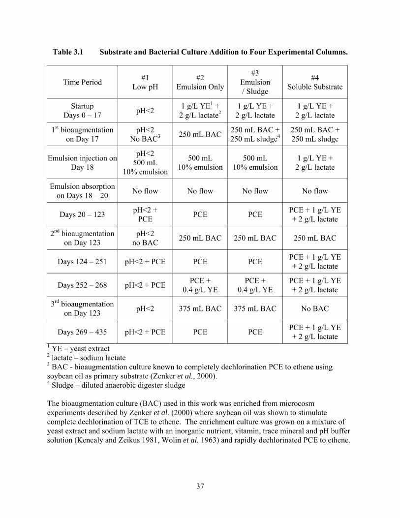
37

Table 3.1 Substrate and Bacterial Culture Addition to Four Experimental Columns.

Time Period #1 Low pH

#2 Emulsion Only

#3 Emulsion / Sludge

#4 Soluble Substrate

Startup Days 0 – 17 pH<2 1 g/L YE1 +

2 g/L lactate2 1 g/L YE + 2 g/L lactate

1 g/L YE + 2 g/L lactate

1st bioaugmentation on Day 17

pH<2 No BAC3 250 mL BAC 250 mL BAC +

250 mL sludge4250 mL BAC + 250 mL sludge

Emulsion injection on Day 18

pH<2 500 mL

10% emulsion

500 mL 10% emulsion

500 mL 10% emulsion

1 g/L YE + 2 g/L lactate

Emulsion absorption on Days 18 – 20 No flow No flow No flow No flow

Days 20 – 123 pH<2 + PCE PCE PCE PCE + 1 g/L YE

+ 2 g/L lactate

2nd bioaugmentation on Day 123

pH<2 no BAC 250 mL BAC 250 mL BAC 250 mL BAC

Days 124 – 251 pH<2 + PCE PCE PCE PCE + 1 g/L YE + 2 g/L lactate

Days 252 – 268 pH<2 + PCE PCE + 0.4 g/L YE

PCE + 0.4 g/L YE

PCE + 1 g/L YE + 2 g/L lactate

3rd bioaugmentation on Day 123 pH<2 375 mL BAC 375 mL BAC No BAC

Days 269 – 435 pH<2 + PCE PCE PCE PCE + 1 g/L YE + 2 g/L lactate

1 YE – yeast extract 2 lactate – sodium lactate 3 BAC - bioaugmentation culture known to completely dechlorination PCE to ethene using soybean oil as primary substrate (Zenker et al., 2000). 4 Sludge – diluted anaerobic digester sludge The bioaugmentation culture (BAC) used in this work was enriched from microcosm experiments described by Zenker et al. (2000) where soybean oil was shown to stimulate complete dechlorination of TCE to ethene. The enrichment culture was grown on a mixture of yeast extract and sodium lactate with an inorganic nutrient, vitamin, trace mineral and pH buffer solution (Kenealy and Zeikus 1981, Wolin et al. 1963) and rapidly dechlorinated PCE to ethene.

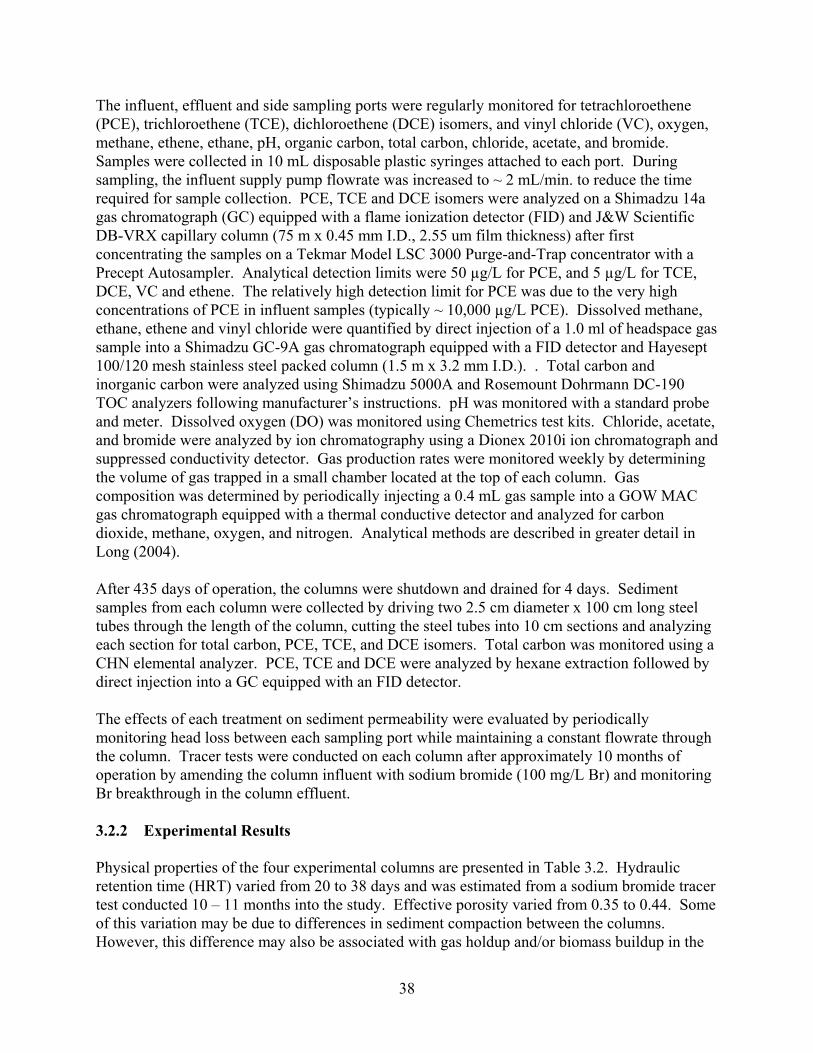
38

The influent, effluent and side sampling ports were regularly monitored for tetrachloroethene (PCE), trichloroethene (TCE), dichloroethene (DCE) isomers, and vinyl chloride (VC), oxygen, methane, ethene, ethane, pH, organic carbon, total carbon, chloride, acetate, and bromide. Samples were collected in 10 mL disposable plastic syringes attached to each port. During sampling, the influent supply pump flowrate was increased to ~ 2 mL/min. to reduce the time required for sample collection. PCE, TCE and DCE isomers were analyzed on a Shimadzu 14a gas chromatograph (GC) equipped with a flame ionization detector (FID) and J&W Scientific DB-VRX capillary column (75 m x 0.45 mm I.D., 2.55 um film thickness) after first concentrating the samples on a Tekmar Model LSC 3000 Purge-and-Trap concentrator with a Precept Autosampler. Analytical detection limits were 50 µg/L for PCE, and 5 µg/L for TCE, DCE, VC and ethene. The relatively high detection limit for PCE was due to the very high concentrations of PCE in influent samples (typically ~ 10,000 µg/L PCE). Dissolved methane, ethane, ethene and vinyl chloride were quantified by direct injection of a 1.0 ml of headspace gas sample into a Shimadzu GC-9A gas chromatograph equipped with a FID detector and Hayesept 100/120 mesh stainless steel packed column (1.5 m x 3.2 mm I.D.). . Total carbon and inorganic carbon were analyzed using Shimadzu 5000A and Rosemount Dohrmann DC-190 TOC analyzers following manufacturer’s instructions. pH was monitored with a standard probe and meter. Dissolved oxygen (DO) was monitored using Chemetrics test kits. Chloride, acetate, and bromide were analyzed by ion chromatography using a Dionex 2010i ion chromatograph and suppressed conductivity detector. Gas production rates were monitored weekly by determining the volume of gas trapped in a small chamber located at the top of each column. Gas composition was determined by periodically injecting a 0.4 mL gas sample into a GOW MAC gas chromatograph equipped with a thermal conductive detector and analyzed for carbon dioxide, methane, oxygen, and nitrogen. Analytical methods are described in greater detail in Long (2004). After 435 days of operation, the columns were shutdown and drained for 4 days. Sediment samples from each column were collected by driving two 2.5 cm diameter x 100 cm long steel tubes through the length of the column, cutting the steel tubes into 10 cm sections and analyzing each section for total carbon, PCE, TCE, and DCE isomers. Total carbon was monitored using a CHN elemental analyzer. PCE, TCE and DCE were analyzed by hexane extraction followed by direct injection into a GC equipped with an FID detector. The effects of each treatment on sediment permeability were evaluated by periodically monitoring head loss between each sampling port while maintaining a constant flowrate through the column. Tracer tests were conducted on each column after approximately 10 months of operation by amending the column influent with sodium bromide (100 mg/L Br) and monitoring Br breakthrough in the column effluent. 3.2.2 Experimental Results Physical properties of the four experimental columns are presented in Table 3.2. Hydraulic retention time (HRT) varied from 20 to 38 days and was estimated from a sodium bromide tracer test conducted 10 – 11 months into the study. Effective porosity varied from 0.35 to 0.44. Some of this variation may be due to differences in sediment compaction between the columns. However, this difference may also be associated with gas holdup and/or biomass buildup in the

39

columns which reduced the pore space available for water movement. Gas production was highest in column #3 which had the lowest effective porosity (0.35). Column #1 had the lowest gas production rate (~ zero) and the highest effective porosity (0.44).

Table 3.2 Operating Conditions of Four Experimental Columns.

#1 Low pH

#2 Emulsion

Only

#3 Emulsion /

Sludge

#4 Soluble Substrate

Average Flow Rate 100 mL/d 107 148 108

Hydraulic Retention Time 38 d 33 d 20 d 30 d

Effective Porosity 0.44 0.42 0.35 0.38 The sediment used to pack the columns was a fine clayey sand (D50 = 0.38 mm, D10 = 0.09 mm, D60/D40 = 3.9, 6.9 % passing #200 sieve) with an initial organic carbon content of 0.00025 g/g and a maximum oil retention capacity of 0.0054 g oil/g sediment (Coulibaly et al. 2006). 50 mL of oil were injected into columns 1, 2 and 3 or 0.0036 g oil/g sediment. Over 99% of the injected oil was retained in the columns increasing the effective organic carbon content of columns #1, #2, and #3 to 0.003 g/g, a factor of twelve increase above background. 3.2.2.1 Indicator Parameters Figure 3.1 shows the observed variation in pH, dissolved oxygen (DO), total organic carbon (TOC) and dissolved methane in the effluent of columns #1 - #4 with time. In column #1 (low pH), the pH declined from 4 to 2.5 at around 150 days. DO in column #1 was initially around 1 mg/L and then increased to levels similar to the influent concentration (2 – 4 mg/L) once biological activity was suppressed by the low pH. In the three live columns (#2, #3, #4), pH was relatively constant at 6 – 7 and DO at or below the effective detection limit of 0.1 mg/L. There was a small increase in chloride in the live columns due to reductive dechlorination of PCE. However, the observed increase in chloride was not a reliable indicator of dechlorination activity due to the high levels of chloride in the influent solution.

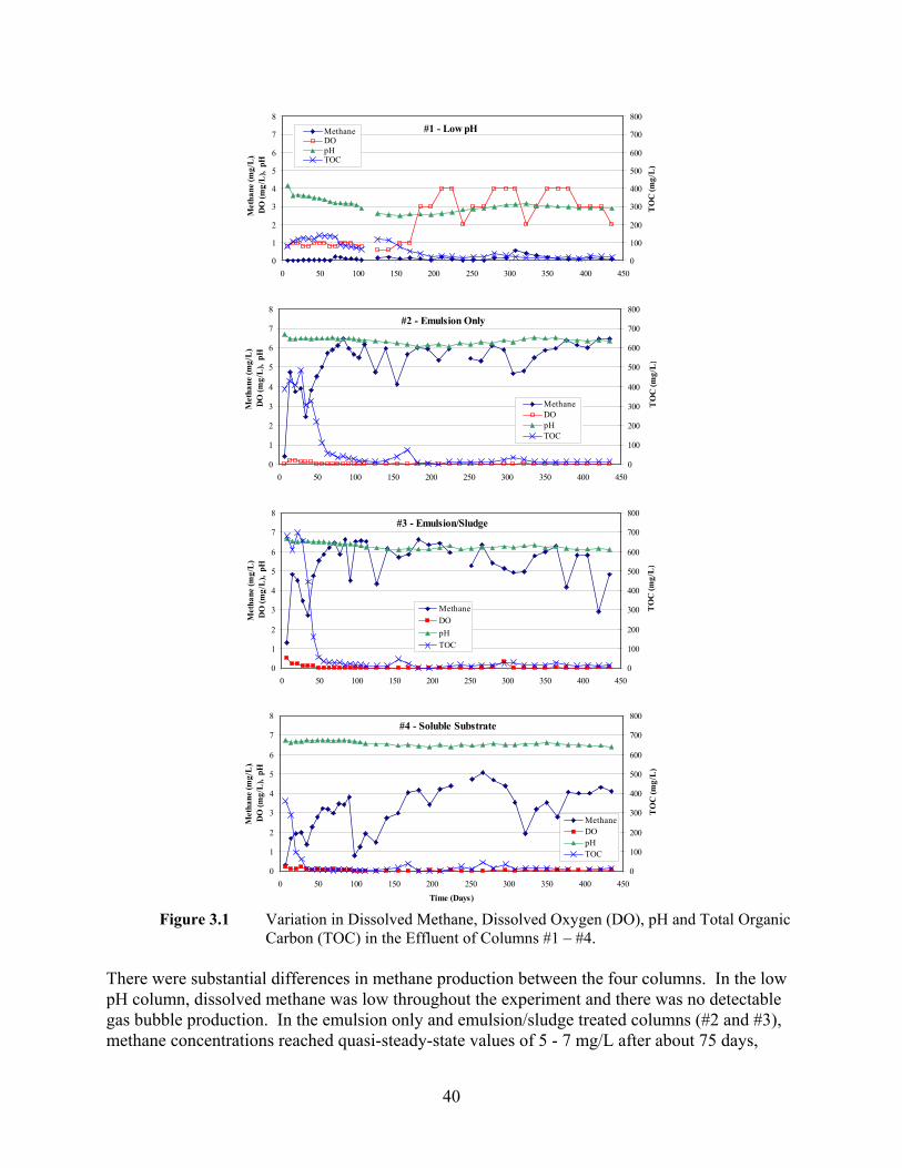
40

#1 - Low pH

0

1

2

3

4

5

6

7

8

0 50 100 150 200 250 300 350 400 450

Met

hane

(mg/

L),

DO

(mg/

L),

pH

0

100

200

300

400

500

600

700

800

TO

C (m

g/L

)

MethaneDOpHTOC

#2 - Emulsion Only

0

1

2

3

4

5

6

7

8

0 50 100 150 200 250 300 350 400 450

Met

hane

(mg/

L),

DO

(mg/

L),

pH

0

100

200

300

400

500

600

700

800

TO

C (m

g/L

)

MethaneDOpHTOC

#3 - Emulsion/Sludge

0

1

2

3

4

5

6

7

8

0 50 100 150 200 250 300 350 400 450

Met

hane

(mg/

L),

DO

(mg/

L),

pH

0

100

200

300

400

500

600

700

800

TO

C (m

g/L

)

MethaneDOpHTOC

#4 - Soluble Substrate

0

1

2

3

4

5

6

7

8

0 50 100 150 200 250 300 350 400 450Time (Days)

Met

hane

(mg/

L),

DO

(mg/

L),

pH

0

100

200

300

400

500

600

700

800

TO

C (m

g/L

)

MethaneDOpHTOC

Figure 3.1 Variation in Dissolved Methane, Dissolved Oxygen (DO), pH and Total Organic

Carbon (TOC) in the Effluent of Columns #1 – #4. There were substantial differences in methane production between the four columns. In the low pH column, dissolved methane was low throughout the experiment and there was no detectable gas bubble production. In the emulsion only and emulsion/sludge treated columns (#2 and #3), methane concentrations reached quasi-steady-state values of 5 - 7 mg/L after about 75 days,

41

while dissolved methane concentrations in the soluble substrate column effluent were somewhat lower (2 – 5 mg/L). Average gas production was 2.0 mL/week (75 - 85% CH4) in column #2, 2.2 mL/week (63 - 81% CH4) in column #3, and 1.4 mL/week (40 - 47% CH4) in column #4. The similar levels of methane produced in columns #2 and #3 suggest that some factor other than the initial inoculum was limiting methanogenesis. The lower methane production from the soluble substrate column is likely due to the smaller amount of substrate added and more oxidized nature of the substrate. The ratio of carbon to oxygen in lactate is 1:1 while the carbon to oxygen ratio in soybean oil is approximately 10:1. As a consequence, methanogenic fermentation of soybean oil can be expected to produce more methane and less carbon dioxide than lactate. Variations in effluent TOC were closely related to biological activity. In the two live emulsion treated columns (#2 and #3), TOC concentrations were initially between 400 and 700 mg/L and then stabilized at between 10 and 25 mg/L with the onset of methane production. The high initial TOC concentrations are believed to be due to microbial activity since the aqueous solubility of soybean oil is reported to be less than 10 mg/L (Pfeiffer, 2003). In the low pH column, TOC varied between 120 and 140 mg/L over the first 150 days and then declined to 10 - 25 mg/L for the remainder of the experiment. The elevated TOC levels during the first 150 days may have been associated with incomplete suppression of biological activity. TOC concentrations in the soluble substrate column (#4) followed the same general pattern as in the two live emulsion columns with effluent TOC levels dropping to between 10 – 20 mg/L with the onset of methane production. 3.2.2.2 Chlorinated Ethenes in Effluent Figure 3.2 shows observed concentrations of PCE, TCE, cis-DCE, VC and ethene in the effluent of columns #1 – #4 over the experimental period. Ethane was not detected in significant concentrations at any time. In column #1 (low pH), TCE began to appear in the column effluent at around 100 days, presumably due to incomplete inhibition of biological activity. However by 200 days, TCE concentrations declined and PCE was, by far, the dominant ethene in the effluent. PCE concentrations in the column #1 effluent gradually increased with time, eventually reaching approximately half the influent concentration by the end of the experimental period at 435 days.

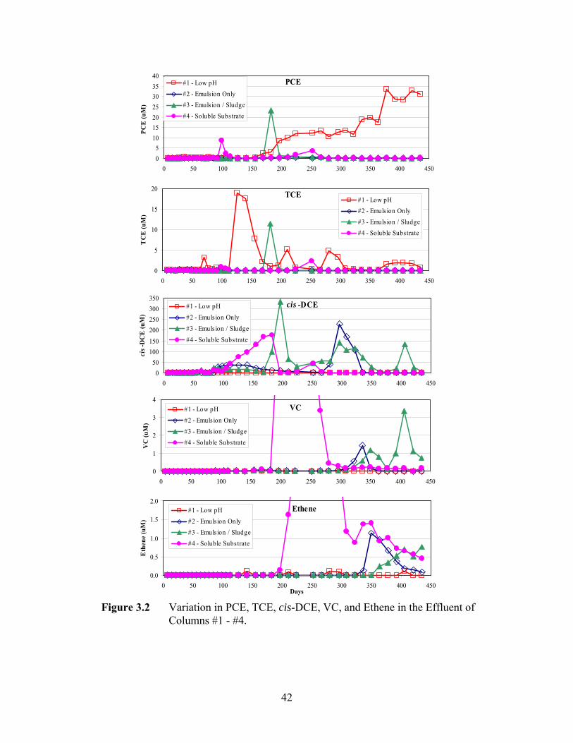
42

PCE

05

10152025303540

0 50 100 150 200 250 300 350 400 450

PCE

(uM

)

#1 - Low pH#2 - Emuls ion Only#3 - Emuls ion / Sludge#4 - Soluble Substrate

TCE

0

5

10

15

20

0 50 100 150 200 250 300 350 400 450

TC

E (u

M)


cis -DCE

050

100150200250300350

0 50 100 150 200 250 300 350 400 450

cis-

DC

E (u

M)


VC

0

1

2

3

4

0 50 100 150 200 250 300 350 400 450

VC

(uM

)


Ethene

0.0

0.5

1.0

1.5

2.0

0 50 100 150 200 250 300 350 400 450Days

Eth

ene

(uM

)

#1 - Low pH#2 - Emulsion Only#3 - Emulsion / Sludge#4 - Soluble Substrate

Figure 3.2 Variation in PCE, TCE, cis-DCE, VC, and Ethene in the Effluent of

Columns #1 - #4.

43

In the column #2 (emulsion only) effluent, PCE and TCE concentrations were at or below the analytical detection limit over the experimental period. cis-DCE broke through in the emulsion only effluent at around 90 days and then remained constant at concentrations comparable to the amount of PCE in the influent indicating relatively efficient conversion of PCE to TCE to cis-DCE. However VC concentrations remained low (< 0.03 μmol/L) and there was no evidence of appreciable ethene production. Similar results were obtained for columns #3 and #4. To stimulate complete reductive dechlorination of cis-DCE to ethene, each of the live columns received 250 mL of bioaugmentation culture on day 123. This treatment was effective in stimulating complete reductive dechlorination in column #4 (soluble substrate) but did not result in complete dechlorination to ethene in the columns #2 and #3 (cis-DCE remained high; VC remained < 0.08 μmol/L, no significant ethene production). On day 252, a 400 mg/L solution of yeast extract was introduced into columns #2 and #3 for 14 days, followed by 375 mL of bioaugmentation culture on day 268. Immediately following bioaugmentation, the yeast extract feed to columns #2 and #3 was discontinued. The final treatment of yeast extract and bioaugmentation culture was successful in stimulating complete dechlorination in column #2. Around day 300, there was a dramatic increase in cis-DCE in the column #2 effluent followed by a rapid decline in cis-DCE, temporary production of VC, followed by production of ethene. By day 400, TCE, cis-DCE and VC were below detection with significant amounts of ethene present in the column effluent. The high DCE concentration observed in the column #2 effluent around day 300 was well in excess of the influent PCE concentration (on a molar basis). The large pulse of cis-DCE released is likely due to the biotransformation of PCE and/or TCE that had sorbed to the residual soybean oil. The dramatic increase in microbial activity may be due to injection of yeast extract solution from day 252 to 268 or due to bioaugmentation on day 268. After 435 days of operation, column #2 continued to reduce PCE, TCE, cis-DCE and VC to below detection with production of some ethene. In column #3 (emulsion/sludge), results were generally similar to column #2. PCE and TCE concentrations were low throughout the experimental period, with the exception of a temporary breakthrough on day 182. One week later, PCE and TCE had declined with a large increase in cis-DCE. As in the emulsion only column, bioaugmentation of column #3 at 123 days appears to have stimulated conversion of some PCE or TCE trapped in the column but did not result in significant VC or ethene production. However, injection of yeast extract and bioaugmentation culture on day 268 did stimulate conversion of cis-DCE to VC and ethene. Around day 320, we observed significant levels of VC in the column 3 effluent followed by significant ethene production at day 400. By the end of the 435 day operating period, VC and ethene concentrations had increased in the column #3 effluent. However, cis-DCE concentrations remained high indicating that the emulsion/sludge treatment was not completely effective in transforming PCE to non-toxic end-products. The less complete conversion of cis-DCE in this column is likely associated with the addition of anaerobic digester sludge to this column. Lee et al. (2004) showed that changes in the relative distribution of the different trophic groups (PCE and cis-DCE dehalogenators, methanogens, and different fermenter groups) in the initial inoculum can have a substantial impact on the amount of ethene produced and the fraction of H2

44

used for methane production. The shorter HRT for column #3 (~ 20 days) compared to column #2 (~ 33 days) may also have contributed to less efficient conversion of cis-DCE. In column #4 (soluble substrate), results were generally similar to column #2 (emulsion only). In column #4, cis-DCE exceeded 10 μmol/L on day 84 and then steadily increased to over 606 μmol/L on day 184. The rapid increase in DCE after day 100, may be due to a second bioaugmentation of column #4 on day 123. Immediately following the decrease in cis-DCE on day 184, we observed a temporary increase in VC (maximum of 9.7 μmol/L) followed by an increase in ethene (maximum of 9 μmol/L). Column #4 provided very effective treatment up to day 435 with PCE, TCE, DCE and VC degraded to below the analytical detection limit. 3.2.2.3 Final Chloroethene and Total Carbon Distribution in Sediment At the completion of the 14 month experimental period, two 2.5 cm diameter steel tubes were driven through each column to collect sediment samples for analysis of sediment associated PCE, TCE, cis-DCE and total carbon (TC). One tube was cut into 10 cm sections and analyzed for chloroethenes while the second was sectioned and analyzed for total carbon. In many cases, sediment samples were not recovered from the full length of the column. As a consequence, the number and location of samples analyzed for chloroethenes and TC vary. Analytical results for PCE, TCE, and cis-DCE in sediment samples from each column are summarized in Table 3.3. There were no significant trends in PCE, TCE or cis-DCE concentration with distance in any column (data not shown). Substantial amounts of PCE were found in sediment from column #1 due to inhibition of biological activity by the low pH. Sorption was much less significant in columns #2, #3 and #4 due to the rapid conversion of PCE to cis-DCE and the much higher solubility of cis-DCE. Table 3.3 PCE, TCE and cis-DCE Concentration in Column Sediment after 435 Days

Operation.

PCE (µg/g) TCE (µg/g) cis-DCE (µg/g) n

Ave. Std. dev Range Ave. Std.

Dev. Range Ave. Std. Dev. Range

#1 – Low pH 9 6.1 5.8 0.017 -13.472 0.004 0.007 0 - 0.020 0.024 0.012 0.018 -

0.055

#2 - Emulsion Only 7 0.002 0.004 0 - 0.010 0.003 0.008 0 - 0.022 0.015 0.006 0.001 -

0.019

#3 - Emulsion / Sludge 4 0.16 0.31 0 - 0.620 0 0 0 – 0 1.0 2.0 0 - 4.025

#4 - Soluble Substrate 9 0.16 0.47 0 - 1.402 0.02 0.07 0 - 0.205 0.01 0.01 0 - 0.029

45

Total carbon (TC) concentrations in sediment samples from each column corrected for background are summarized in Table 3.4. Several samples from column #1 had higher TC concentrations than equivalent samples from the other three columns. However, the average TC concentration was highest in column #3 due to a single sample with a very high TC concentration (15.86 mg/g) collected immediately adjoining the column inlet. There was no statistically significant difference in the mean TC concentration of the columns. However, TC concentrations in all four columns were significantly higher than background concentration of 0.25 mg/g (α < 0.05). The relatively low levels of TC in the sediment is not surprising given that a relatively small amount of emulsion was injected in columns #1, #2 and #3 (~3 mg of organic carbon per gram of sediment).

Table 3.4 Sediment Carbon Content above Background in Columns after 435 Days Operation*.

Total Carbon (mg/g)

n Ave. Std. dev Range

#1 - Low pH 8 1.7 1.2 0.75 – 4.55

#2 - Emulsion Only 8 0.6 0.6 0.15 – 2.05

#3 - Emulsion / Sludge 8 2.6 5.4 0.25 – 15.85

#4 – Soluble Substrate 8 0.9 0.8 0.25 – 2.35

* All samples were corrected for the background carbon content of 0.25 mg/g. 3.2.2.4 Chloroethene Mass Balance An overall mass balance for total ethenes was developed for each column by comparing the mass injected with the cumulative mass in the effluent and mass sorbed to the sediment at the end of the experimental period (Table 3.5). Total ethenes were calculated as the sum of PCE, TCE, DCE isomers, VC, ethene and ethane. However, concentrations of trans-DCE, 1,1-DCE and ethane were very low.

46

Table 3.5 Total Ethenes Mass Balance Results.

In (μmol)

Out (μmol)

Sediment (μmol)

Error (μmol)

Error (%)

#1 - Low pH 1353 635 474 244 18

#2 - Emulsion Only 2408 1374 2.4 1032 43

#3 – Emulsion / Sludge 4511 4339 145 27 1

#4 – Soluble Substrate 2009 2903 16 -910 -45

Overall mass balance errors were reasonable for columns #1 and #3 (18% and 9%). However, mass balance errors for columns #2 and #4 were significantly higher and were likely due to loss of ethene in gas bubbles released from the columns. Ethene was periodically detected in the gas released from these columns at levels ranging from 200 to 1000 ppm. However, ethene concentrations in the gas were not routinely monitored and so could not be included in the mass balance calculation. Some portion of the unaccounted for ethene could also result from conversion to carbon dioxide or methane as described by Bradley (2003). The cumulative mass of total dissolved ethenes in the influent and effluent of each column are shown in Figure 3.3. Cumulative mass was calculated as the sum of measured concentration times the volume of water injected since the previous chemical analysis. Total ethenes discharged in the column #1 (low pH) effluent were less than the total influent load due to sorption to oil trapped within the column. However, most of this material was recovered as PCE associated with sediment.

47

#1 - Low pH

0

1000

2000

3000

4000

5000

0 50 100 150 200 250 300 350 400 450

Tota

l Eth

. (um

ol)

A

#2 - Emulsion Only

0

1000

2000

3000

4000

5000

0 50 100 150 200 250 300 350 400 450

Tota

l Eth

.(um

ol)

B

#3 - Emulsion/Sludge

0

1000

2000

3000

4000

5000

0 50 100 150 200 250 300 350 400 450

Tota

l Eth

. (um

ol)

C

#4 - Soluble Substrate

0

1000

2000

3000

4000

5000

0 50 100 150 200 250 300 350 400 450Days

Tota

l Eth

. (um

ol)

D

Figure 3.3 Cumulative Mass of Total Dissolved Ethenes in the Influent (solid line)

and Effluent (dashed line) of Columns #1 - #4. In column #2, the mass of total dissolved ethenes in the influent was much greater than in the effluent over the first 270 days. This difference indicates that ethenes were being stored in the column and is consistent with sorption of the more chlorinated species (PCE and TCE) to the entrapped soybean oil. Around day 270, a rapid increase in effluent ethene mass was observed due to high concentration of cis-DCE being released. However after day 350, total ethenes

48

concentrations in the effluent remained low and influent mass remained greater than that in the effluent. By the end of the experiment, the cumulative mass of total dissolved ethenes in the influent was significantly greater than in the effluent (Table 4). This difference is believed to be due to release of ethene in gas bubbles which is not included in the overall mass balance calculation. The total amount of chloroethenes recovered in the sediment at the end of the experiment was less than 0.1% of the influent mass indicating that sorption to the sediment was negligible. Trends in cumulative total ethenes in column #3 followed the same general trends as in column #2. For the first 200 days, cumulative ethene mass in the influent is greater than the effluent, which is consistent with sorption of PCE and/or TCE to the entrapped soybean oil. Around day 200, there is a rapid increase in total ethenes in the effluent due to high concentrations of cis-DCE released. By day 225, cumulative ethenes in the effluent are approximately equal to those in the influent. From that point on, total ethenes are released from column #3 at approximately the same rate that they enter the column. A minor difference between total dissolved ethenes in the influent and effluent is observed towards the end of the experimental period when column #3 begins to release significant amounts of ethene in gas bubbles. The mass of total dissolved ethenes introduced into column #4 exceeded the effluent mass until day 112, when large amounts of cis-DCE began to be released from the column. This indicates that sorption was significant in column #4, but not to the extent observed in columns #2 and #3. Total ethenes in the column #4 effluent were approximately equal to the influent from day 168 until day 210 when ethene release in gas bubbles became significant. 3.2.2.5 Carbon Mass Balance A carbon mass balance for each column is presented in Table 3.6 including injected organic substrate and effluent methane, organic carbon, and inorganic carbon. Methane and carbon dioxide released from the columns as gas bubbles was not included in this analysis because of limited data on gas composition. However, the gas composition data that is available indicates the amount of carbon in the gas bubbles released from columns #2, #3 and #4 was between 0.08 and 0.13 g carbon or less than 1% of the organic carbon injected. Overall mass balance errors were highly variable ranging from 2% in column #3 to 67% in column #2. The large mass balance errors are believed to be due to poor recovery of sediment cores and the high associated uncertainty in the amount of organic carbon present in the sediment at the completion of the experiment.

49

Table 3.6. Carbon Mass Balance Results for Columns #1 – #4.

#1 – Low pH

#2 – Emulsion Only

#3 – Emulsion /

Sludge

#4 – Soluble

Substrate

g % g % g % g %

Injected – Total Carbon 38.7 100 38.7 100 38.7 100 10.3 100

Effluent – Methane 0.005 0 0.19 0.5 0.27 0.7 0.11 1.1

Effluent - Organic Carbon 1.853 4.8 2.59 6.7 2.31 6 0.99 16

Effluent - Inorganic Carbon 0.027 0.1 2.20 5.7 1.94 5 1.67 9.6

Sediment Total Carbon* 21 55 7.6 20 33 86 11 107

Sum Effluent / Sediment 23 60 13 33 38 98 14 133

Unaccounted for Carbon 16 40 26 67 1 2 -3 -33

* Total carbon present in the sediment at the end of the experiment corrected for initial sediment carbon concentration. Column #1 released only 4.9% of the injected carbon over the 14 month monitoring period indicating that, in the absence of biological activity, edible oil emulsions can be retain by sandy sediments for extended periods. Total carbon released from the two live emulsion treated columns (#2 and #3) was 12 to 14% of the injected carbon. The higher levels of inorganic carbon, organic carbon and methane in the two live emulsion columns compared to column #1 indicates that biological activity can significantly enhance carbon release from entrapped oil. Total carbon in the column #4 sediment was significantly higher than initial concentrations indicating that a large portion of the soluble substrate was retained in the column, presumably as cell biomass. 3.2.2.6 Permeability Loss in Columns One of the major concerns associated with the use of edible oil emulsions for aquifer bioremediation has been the potential impact on aquifer permeability. The effective hydraulic conductivity of each column was periodically monitored to evaluate the potential for aquifer clogging by oil droplets, biomass and/or trapped gas bubbles. Hydraulic conductivity (K) was determined by measuring the head loss between the column effluent and each sampling port while maintaining a constant flow rate. Figure 3.4 shows the variation in the measured K divided by the initial hydraulic conductivity (Ko) over the experimental period. The value plotted at zero months is the K/Ko immediately following emulsion injection.

50

0.01

0.1

1

10

-2 0 2 4 6 8 10 12 14Months after Injection

K/K

o

#1 - Low pH#2 - Emulsion Only#3 - Emulsion/Sludge#4 -Soluble Substrate

Figure 3.4. Change in Relative Permeability (K/Ko) from Inlet to Outlet during Column

Operation. There was no significant change in the hydraulic conductivity of column #1 (low pH) over the monitoring period, indicating that emulsion injection in the absence of biological activity did not result in appreciable clogging of the aquifer sediment. This is not surprising given the very small amount of oil injected (~3 mg C/g) which would occupy less than 2% of the sediment pore space. The minor variations in K shown in Figure 3.4 for column #1 were likely due to difficulties associated with measuring small variations in head over the 1 m long column at low flowrates. In column #2 (emulsion only), the effective hydraulic conductivity declined following emulsion injection and then recovered to near the preinjection value at the 13 month measurement. In column #3 (emulsion and sludge), permeability loss was greater and did not recover, possibly due to the greater biological activity associated with addition of the anaerobic digester sludge. Permeability loss was greatest in the soluble substrate fed column, presumably due to the large amount of readily biodegradable substrate available to the microorganisms. Figure 3.5 shows the variation in K between the different sampling ports after 13 months of column operation. Hydraulic conductivity was essentially constant along the length of column #1. Again, the minor variations shown for column #1 in Figure 5 are likely associated with the limited precision of the K measurements. In the three live columns, essentially all of the permeability loss occurred between the inlet and the first sampling port, presumably associated with biomass growth.

51

0.01

0.10

1.00

10.00

100.00

0 25 50 75 100

Location along Column (cm)

K (m

/d)

#1 - Low pH#2 - Emulsion Only#3 - Emulsion/Sludge#4 - Soluble Substrate

Figure 3.5. Variation in Hydraulic Conductivity (K) along the Length of the Column after 13

Months of Operation. 3.2.3 Implications for Full-Scale Edible Oil Barriers Experimental results from this work have shown that a single injection of emulsified soybean oil can be effective in enhancing reductive dechlorination. However, this study also raised a number of important issues related to the design and performance of full-scale edible oil barriers. 3.2.3.1 Growth of Dechlorinating Microorganisms Soybean oil emulsion appears to be effective in enhancing reduction of PCE to cis-DCE but additional nutrients may be required to stimulate rapid growth of microorganisms that can reduce cis-DCE to ethene. In columns #2 and #3, a single injection of yeast extract, lactate and soybean oil emulsion combined with bioaugmentation on days 0 and 123 was effective in enhancing reduction of PCE to cis-DCE. However, there was minimal conversion of cis-DCE to VC and ethene in these columns over the first 250 days of operation. In contrast, there was extensive production of VC and ethene after 200 days in column #4 which received 1 g/L yeast extract and 2 g/L sodium lactate and the same bioaugmentation treatments. Once columns #2 and #3 where treated with 0.4 g/L yeast extract for 14 days followed by a third addition of a bioaugmentation culture, VC and ethene production increased. These results suggest that inorganic nutrients, vitamins, amino acids or other materials present in yeast extract, but absent from soybean oil, may be required for effective growth of microorganisms that can dechlorinate cis-DCE to VC and ethene. However, once an active population of dechlorinators is established, this population can be sustained for over 160 days without addition of more yeast extract. These observations are consistent with prior work by Maymo´ - Gatell et al. (1997) who found that filter-sterilized anaerobic digester sludge supernatant and yeast extract stimulated VC and ethene production by Dehalococcoides ethenogenes strain 195. The stimulatory effects of the yeast extract may be, in part, due to the specific experimental conditions of this work. The column influents in our work

52

contained PCE in a CaCl2 solution with no other nutrients. Groundwater typically contains some nitrate and phosphate, which could serve as an inorganic nutrient source. 3.2.3.2 Substrate Life Monitoring results obtained over the 14 month duration of the column study indicate that a single injection of emulsified soybean oil can provide a long-term source of organic carbon to support anaerobic biodegradation processes. Both columns #2 and #3 showed very good performance, with no evidence of substrate depletion or reduced degradation rates after 14 months of operation. However, it is not possible to accurately estimate the effective operating life of a single emulsion injection with the available data. At the end of 14 months of operation, columns #2 and #3 were releasing approximately 1% of the injected carbon per month as inorganic carbon, organic carbon, and dissolved methane. At this rate, all of the injected carbon would be released in 6 to 7 years. However, the effective operating life is expected to be significantly less since some carbon was also being released as gas bubbles. More importantly, pollutant removal efficiency can be expected to decline before the injected carbon is completely depleted. Once treatment efficiency drops below required levels, additional emulsion would need to be injected to maintain performance. 3.2.3.3 Required Contact Time High concentrations of PCE (15 – 20 mg/L) were degraded to below the analytical detection limit in column #2 which was treated with emulsified soybean oil and had a 33 day hydraulic retention time (HRT). However, PCE conversion was less efficient in column #3 which was treated with emulsified soybean oil and anaerobic digester sludge and had a 20 day HRT. The reason for the lower removal efficiency in column #3 is not known but may be related to the shorter HRT and/or greater competition for H2 by the larger methanogen population. In the field, the extent of competition will likely vary from site to site. Under these conditions, it may be desirable to generate emulsion treated zones that provide at least a 30 day HRT. For a groundwater flow velocity of 0.1 m/d, this would require a 3 m wide emulsion treated zone. 3.2.3.4 Hydrophobic Partitioning to Oil The effect of chlorinated ethene partitioning to the soybean oil on contaminant migration rates can be approximated using a retardation factor (R) approach where R is the ratio of the contaminant transport velocity to the non-reactive solute transport velocity. In this work, we assume sorption to the background organic carbon is negligible and calculate R using equation 1

R = 1 + ρB fo KP / ε0 (1) where ρB is the sediment bulk density, fo is the organic carbon fraction associated with the oil, KP is the oil-water partition coefficient, and ε0 is porosity. Estimated retardation factors for conditions representative of column #1 (ρB = 1.48 g/cm3, fo = 0.0028 g/g, and ε0 = 0.44) are shown in Table 3.7. KP values are from Pheiffer (2003) who examined the partitioning of PCE, TCE, cis-DCE, and VC between water and soybean oil at 20 °C.

Table 3.7. Retardation of Chloroethenes in a Typical Edible Oil Barrier.

53

Parameter PCE TCE cis-DCE VC Kp (from Pheiffer, 2003) 1240 338 61 22

R (estimated from Eq. 1) 12.7 4.2 1.6 1.2 Travel time through a 3 m barrier* 1.0 yr 0.4 yr 0.1 yr 0.1 yr

* assumes non-reactive v = 0.1 m/d Retardation factors estimated using Equation 1 are generally consistent with the column experimental results. In column #1, PCE broke through at approximately 50% of the influent concentration after approximately 14 months or 11 times the HRT which is generally consistent with an estimated retardation factor of 13. However, retardation factors for TCE, cis-DCE and VC are much lower due to the lower Kp values for these compounds. The rapid breakthrough of TCE in Column 1 supports this interpretation. High concentrations of TCE appeared in the column #1 effluent approximately 112 days after the start of PCE injection. This is equivalent to a retardation factor of 3 for TCE, similar to the estimated retardation factor of 4.2. Retardation factors for cis-DCE and VC are much lower indicating that these compounds will not be significantly retained by entrapped soybean oil. Estimated travel times for PCE, TCE, cis-DCE and VC to migrate through a 3 m wide edible oil barrier with a non-reactive solute transport velocity of 0.1 m/d (HRT = 0.08 yr or 1 month) are shown Table 7. In the absence of biological activity, breakthrough of PCE could be delayed by up to a year due to sorption to the entrapped oil. However in practice, hydrophobic sorption will likely be much less significant. As observed in columns #2 and #3, some portion of the PCE and/or TCE may initially partition into the soybean oil. However, once an acclimated microbial community develops, PCE will be converted to more soluble daughter products and these daughter products will rapidly migrate through the barrier. 3.2.3.5 Permeability Effects In the absence of biological activity, injection of soybean oil emulsion did not result in significant permeability loss which is consistent with prior results by Coulibaly and Borden (2004). However, when biological activity is enhanced, permeability loss can occur due to biomass production and/or gas bubble accumulation. In this project, permeability loss was not excessive in the emulsion only column (#2). However, permeability declined by an order of magnitude in the emulsion/sludge treated column (#3). The greater permeability loss in the emulsion/sludge column may be due to the greater biological activity and could explain the high permeability loss observed in the soluble substrate column (#4).

54

Regardless of the substrate used, the effects of biological activity on aquifer permeability need to be carefully considered when planning an enhanced anaerobic bioremediation project. If permeability loss is excessive, contaminated groundwater could flow around the anaerobic treatment zone reducing treatment efficiency. However, field monitoring results from several sites treated with emulsified soybean oil indicate that permeability loss is usually not excessive and the edible oil barriers can perform very well with no evidence of flow bypassing (Zawtocki et al. 2004, FRTR, 2004). 3.3 IDENTIFICATION OF SLOW RELEASE SUBSTRATES FOR ANAEROBIC BIOREMEDIATION 3.3.1 Experimental Methods The anaerobic biodegradation potential of a range of substrates was monitored by incubating 50 mg of the target organic substrate, 5 mL or 1 mL of anaerobic digester sludge (Chapel Hill, North Carolina), and 100 mL of nutrient media [NaHCO3 (3.5 g/L), NH4Cl (1.0 g/L), NaCl (0.9 g/L), MgCl2 (0.2 g/L), CaCl2 (0.1 g/L), KH2PO4 (1.61 g/L), Na2HPO4 (3.19 g/L), cysteine hydrochloride (10 mL/L), resazurin (0.002%)] in 160 serum bottles with thick butyl rubber stoppers at 37°C. Prior to preparation, the media was boiled under oxygen free nitrogen to remove dissolved oxygen. The bottle headspace was flushed with 80% N2 - 20% CO2. All incubations were conducted in triplicate. Substrate biodegradation rate was assayed by monitoring biogas production over time using a wetted glass syringe. Bottles were mixed immediately after construction and before each gas measurement. Gas production results were compared to parallel incubations that did not contain organic substrate. Carbon dioxide and methane production was confirmed by analysis of selected gas samples using a GOW MAC gas chromatograph equipped with a thermal conductive detector (TCD). Intermittent flow column experiments were conducted to evaluate the ability of emulsified liquid soybean oil and emulsified SEFA (S-270) to support reductive dechlorination without excessive methane production and to evaluate the effect of varying sulfate (SO4) levels on pollutant degradation. The experimental system consisted of eighteen 3.8 cm diameter by 30 cm long soil columns. The sediment used to pack the columns was obtained from Dover Air Force Base (AFB) near the location of a full-scale enhanced bioremediation project. The columns were packed with wet sediment in an anaerobic glove box. During the packing procedure, the sediment was frequently tamped to remove any entrapped gas bubbles. The columns were operated in an intermittent flow mode for 14 months where 16-25 mL of influent (~ 0.25 pore volumes) was flushed through the column. The columns were then allowed to rest for 24 hours before the next 0.25 pore volumes were introduced. This resulted in an ‘average’ groundwater velocity of ~7.5 cm/d and hydraulic retention time (HRT) in the columns of ~ 4 days. The influent reservoir for each column was amended with a mixture of pure perchloroethene (PCE) and hexadecane designed to maintain an influent concentration of roughly 10 mg/L PCE. Some columns received 200 mg/L Na2SO4 in the influent to evaluate the effect of high background sulfate levels on substrate longevity and reductive dechlorination. Three columns received dilute HCl (0.01 N) in the influent to inhibit biological activity.

55

Each of the columns was inoculated by one of the following treatments: (1) Live – inject 25 mL of bioaugmentation culture, 12 mL of autoclaved anaerobic digester sludge followed by 25 mL of nutrient media; (2) Live + sludge – inject 25 mL of bioaugmentation culture, 12 mL of live anaerobic digester sludge followed by 25 mL of nutrient media; and (3) Inhibited – inject 21 mL of autoclaved anaerobic digester sludge followed by 41 mL of nutrient media. The different volumes of digester sludge and bioaugmentation culture were calculated to provide the same amount of volatile solids to each column. The bioaugmentation culture was enriched from a site in Lumberton, North Carolina, and was capable of complete dechlorination of PCE to ethene. The digester sludge was added to evaluate substrate longevity in an aquifer with a high number of methanogens. Emulsified soybean oil or S-270 (20 mL of~10% by volume) was injected into each column and then displaced with 40 mL deaired salts solution (100 mg/L CaCl2) to push the emulsion into the column. The column was then allowed to sit for two days, before starting the daily pumping schedule. Effluent samples were collected daily for two weeks and analyzed for volatile solids to determine the amount of emulsion released from the columns. The influent and effluent from each column were periodically monitored for PCE, trichloroethene (TCE), dichloroethene (DCE) isomers, vinyl chloride (VC), oxygen, nitrate, sulfate, methane, ethene, ethane, and pH. PCE, TCE and DCE isomers were analyzed on a Shimadzu 14a gas chromatograph (GC) equipped with a flame ionization detector (FID) after first concentrating the samples on a Tekmar Model LSC 3000 Purge-and-Trap concentrator with a Precept Autosampler. Dissolved methane, ethane, ethene and vinyl chloride were quantified by direct injection of a 1.0 ml of headspace gas sample into a Shimadzu GC-9A gas chromatograph equipped with a FID detector. pH was monitored with a standard probe and meter. Chloride, nitrate and sulfate were analyzed by ion chromatography using a Dionex 2010i ion chromatograph and suppressed conductivity detector. 3.3.2 Substrate Screening Incubations In the first phase of this work, a wide range of organic substrates were examined to identify materials that will generate slow, steady production of CH4 and CO2. We have assumed that biogas production (primarily CH4 and CO2) is proportional to H2 and/or acetate production since these materials are required for CH4 production. H2 and acetate can also be used as electron donors for reductive dechlorination (He et al., 2002). This general approach for assessing anaerobic biodegradability under methanogenic conditions is well established and has been applied by a variety of researchers (Shelton and Tiedje, 1984a; Colleran et al., 1992; Shelton and Tiedje, 1984b; Suflita and Concannon, 1995). Readers should be aware that low biogas production does not necessarily imply that the complex organic substrates were not degraded. If a complex organic substrate was fermented to soluble intermediate products (e.g., long chain fatty acids) that did not degrade further, these partially degraded intermediates would not generate significant biogas. Biogas production is believed to be a reasonable indicator of the potential for use of a substrate for reductive dechlorination since: (a) soluble intermediates that do not degrade further will not produce H2 and acetate; and (b) H2 and/or acetate are the primary substrates used in reductive dechlorination.

56

The amount of biogas produced could also be lower if a substrate produces a larger amount of CO2, since a portion of the CO2 will remain in solution as bicarbonate in the pH buffered media. The amount of carbon potentially converted to CH4 and CO2 can be estimated from the Equation 1 (Buswell and Hatfield, 1936). CnHaOb + (n- a/4 –b/2) H2O (n/2 – a/8 + b/4) CO2 + (n/2 – a/8 + b/4) CH4 (1) The fraction of organic carbon converted to CH4 typically varies between 50% and 70% with a greater percentage of CO2 produced from more oxidized substrates (e.g., acetate, lactate, molasses) and a greater percentage of CH4 produced from the more reduced substrates (e.g., vegetable oils). The more oxidized substrates also provide fewer reducing equivalents to drive reductive dechlorination and consume competing electron acceptors. For example, lactic acid (C3H6O3) can potentially produce 2 moles of H2 per mole carbon (0.066 moles H2 per gram lactic acid) compared to soybean oil (C56.3H99.5O6) which can produce 2.8 moles of H2 per mole carbon (0.18 moles H2 per gram oil) (Solutions-IES, 2006). Cumulative biogas production (ΣG) results from triplicate incubations with no added carbon (blank), chitin, and soybean oil are shown in Figure 3.6. The blank incubations (1 mL inoculum) resulted in a slow, steady production of biogas as the digester sludge inoculum decayed away. The gas production patterns for chitin and soybean oil are typical for substrates where gas production is rapid during the first 100 days, then slows or stops. For chitin, gas production was very reproducible between replicates. In contrast, for soybean oil, there was some variability between replicates during the rapid gas production phase, due to small variations in the lag period between bottles. For most substrates, the cumulative gas production over 300 days was reasonably consistent between replicates.

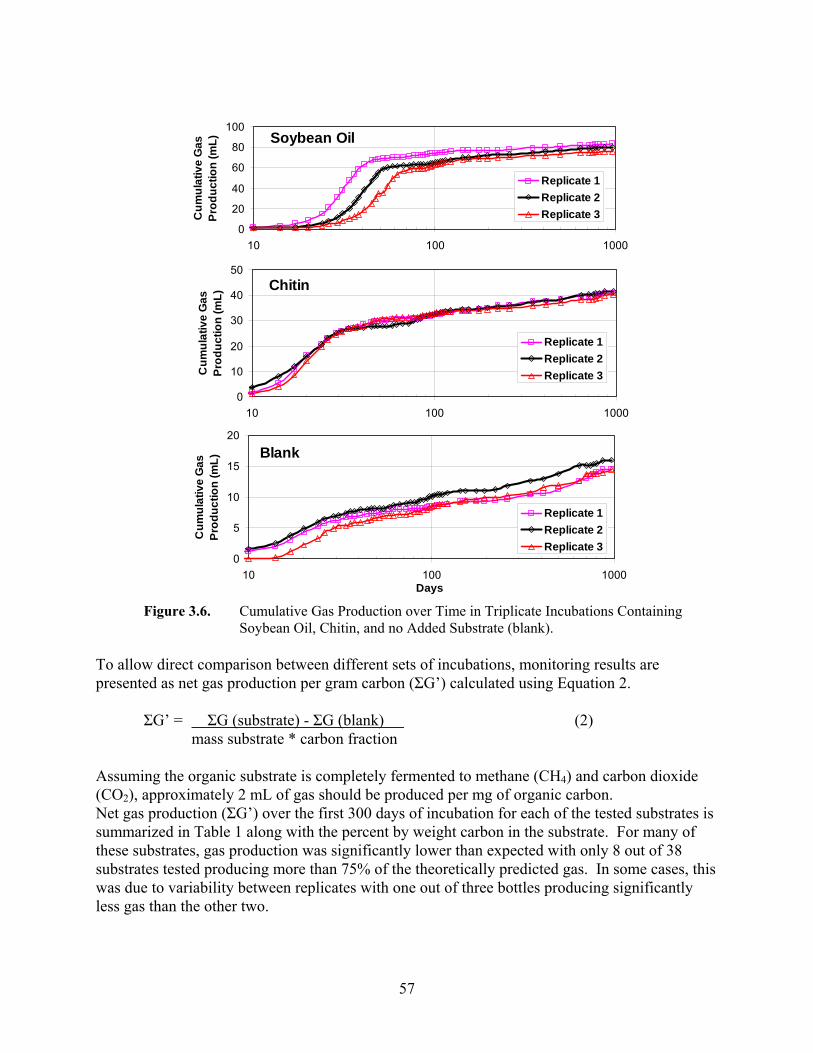
57

Soybean Oil

0

20

40

60

80

100

10 100 1000

Cum

ulat

ive

Gas

Pr

oduc

tion

(mL)

Replicate 1Replicate 2Replicate 3

Chitin

0

10

20

30

40

50

10 100 1000

Cum

ulat

ive

Gas

Pr

oduc

tion

(mL)


Blank

0

5

10

15

20

10 100 1000Days

Cum

ulat

ive

Gas

Pr

oduc

tion

(mL)


Figure 3.6. Cumulative Gas Production over Time in Triplicate Incubations Containing

Soybean Oil, Chitin, and no Added Substrate (blank). To allow direct comparison between different sets of incubations, monitoring results are presented as net gas production per gram carbon (ΣG’) calculated using Equation 2.

ΣG’ = ΣG (substrate) - ΣG (blank) (2) mass substrate * carbon fraction Assuming the organic substrate is completely fermented to methane (CH4) and carbon dioxide (CO2), approximately 2 mL of gas should be produced per mg of organic carbon. Net gas production (ΣG’) over the first 300 days of incubation for each of the tested substrates is summarized in Table 1 along with the percent by weight carbon in the substrate. For many of these substrates, gas production was significantly lower than expected with only 8 out of 38 substrates tested producing more than 75% of the theoretically predicted gas. In some cases, this was due to variability between replicates with one out of three bottles producing significantly less gas than the other two.

58

Table 3.8. Substrates Screened for their Ability to Support Slow, Steady Biogas Production.

300 Day

Net Gas Production (mL/mg carbon)

MATERIAL

Carbon Content

(% by wt.) Mean Std. Dev. Blackstrap Molasses G 32.5 1.54 0.18 Chitin C 44.6 1.13 0.04 Ethyl Lactate O 50.4 2.06 0.06 Sodium Acetate M 29.3 1.44 0.17 Sodium Lactate F 19.5 0.92 0.05 Lauric Acid A 72.3 -0.26 0.08 Myristic Acid A 73.9 1.47 1.42 Stearic Acid A 76.3 0.29 0.18 Canola Oil H 77.8 0.63 0.93 Corn Oil H 77.8 0.21 0.17 Olive Oil A 77.4 1.96 0.32 Soybean Oil D 77.0 1.13 0.02 Expelled Soybean Oil D 77.7 1.58 0.09 Hydrogenated Soybean Oil D 77.3 1.62 0.09 Soy methyl-ester B 77.0 0.16 0.08 Mineral Oil I 86.7 -0.21 0.04 Petrolatum E 86.3 0.00 0.20 Paraffin K 85.3 0.06 0.02 S-1670 L (HLB = 16) 75% mono-ester, 25% di-, tri- and poly-esters 59.3

0.98 0.19

S-970 L (HLB = 9) 50% mono-ester, 50% di-, tri- and poly-esters 62.3

0.93 0.19

S-270 L (HLB = 2) 10% mono-ester, 90% di-, tri- and poly-esters 68.9

0.40 0.01

S-170 L (HLB = 1) 100% di-, tri- and poly-esters 72.7 -0.07 0.03 S-070 L (HLB < 1) 100% di-, tri- and poly-esters 74.1 0.02 0.02 SEFA-5 Soyate J (penta-ester) 73.1 0.25 0.09 SEFA-6 Soyate J (hexa-ester) 74.0 0.21 0.01 SEFA-7 Soyate J (hepta-ester) 75.1 0.15 0.04 SEFA-8 Soyate J (octa-ester) 76.1 -0.02 0.03 SEFA-8 Behenate J (octa-ester) 77.1 0.11 0.01 Ivory Soap J 66.9 1.67 0.02 Actiflo 68-UB D (HLB = 2) 65.5 1.19 0.03 Centrol CA D (HLB = 6) 66.8 1.46 0.05 Blendmax K D (HLB = 8) 66.2 1.60 0.27 Centrolene A D (HLB = 10) 63.9 1.08 0.05

59

300 Day Net Gas Production

(mL/mg carbon) MATERIAL

Carbon Content

(% by wt.) Mean Std. Dev. Centromix E D (HLB = 12) 63.6 1.37 0.03 Centrophase C D (HLB = 4) 68.8 1.16 0.03 Tween 20 N (HLB =16.7) 56.1 0.39 0.04 Tween 21 N (HLB = 13.3) 60.2 0.83 0.03 Tween 85 N (HLB = 11) 63.0 1.07 0.14 Substrate Sources: A Acros Organics, NJ B AG Environmental Products L.L.C. (Soygold 1000) C Aldrich Chemical Company Inc. Milwaukee, WI D Central Soya Chemargy Division. Fort Wayne, IN. E Cheesebrough – Ponds USA Co. Greenwich, CO F Fisher Chemicals - Fisher Scientific. Fair Lawn, NJ G Golding Farms Foods Inc. Winston-Salem, NC H Harris Teeter®. Matthews, NC I K-mart Corporation. Troy, MI J Procter & Gamble Chemicals. New Milford, CT K Royal Oak Sales Inc. Roswell, GA L Ryoto® sugar ester – Mitsubishi-Kagaku Foods Corporation. Tokyo, Japan M Sigma Chemical Co. St. Louis, MO N Uniquema – Imperial Chemical Industries PLC. Wilmington, DE O Vertec Biosolvents Inc. Downers Grove, IL Raw gas production (ΣG) and net gas product (ΣG’) results are shown in Figures 3.7a and 3.7b for four easily degradable substrates (mean of triplicate incubations). A larger inoculum (5 mL) was used in this set of incubations in an effort to reduce the variability in lag time between replicates and resulted in significantly higher gas production from the blank bottles. However, net gas production was similar to results from other incubations with the smaller 1 mL inoculum. Sodium acetate and sodium lactate were rapidly fermented, with zero net gas production after 30 days. Ethyl lactate hydrolyzes in water releasing ethanol and lactate which are then easily fermented. It appears that one of these materials (presumably lactate) was fermented first followed by a lag period and then a second period of rapid gas production. Gas production from molasses also appeared to occur in two stages with a rapid initial release followed by slower gas production for almost one year.

60

CUMULATIVE GAS PRODUCTION

0

20

40

60

80

100

120

0 100 200 300 400Days

Gas

Pro

duct

ion/

mg

of C

arbo

n EthylLactateMolasses

SodiumAcetateSodiumLactateBlank

a

GAS PRODUCTION NORMALIZED TO CARBON CONTENT

-0.5

0.0

0.5

1.0

1.5

2.0

2.5

0 100 200 300 400Days

Net

Gas

Pro

duct

ion

(mL

/ mg

carb

on)

EthylLactate

Molasses

SodiumAcetate

SodiumLactate

b

Figure 3.7. Cumulative gas production versus time for easily biodegradable substrates: (a)

raw gas production; and (b) gas production corrected for gas production in blank and normalized to carbon content of substrate.

3.3.2.1 Gas Production from Fats and Oils Gas production results from incubations with oils and long-chain fatty acids are shown in Figure 3.8. The rate and total amount of gas produced was greatest for olive oil, followed by soybean oil, myristic acid (C13H27COOH), hydrogenated soybean oil and canola oil. Net gas production was much lower or even negative (less than blank) for stearic acid (C13H35COOH), corn oil, soy methyl-ester, paraffin, and lauric acid (C11H23COOH).

61

-0.5

0.0

0.5

1.0

1.5

2.0

0 100 200 300 400

Days

Net

Gas

Pro

duct

ion

(mL

/ mg

carb

on)

Soybean Oil(Raw)Olive Oil

Corn Oil

Canola Oil

Soy Methyl-esterHydrogenatedSoy OilParraffin

Stearic Acid

Myristic Acid

Lauric Acid

Figure 3.8. Normalized net gas production from fats and oils.

Most of this variation is likely associated with toxic inhibition of substrate fermentation by long-chain fatty acids. All animal and vegetable fats and oils are classified as triglycerides and contain three long chain fatty acids esterified to a glycerol core. Under anaerobic conditions, triglycerides are rapidly hydrolyzed, releasing long chain fatty acids and glycerol (Hanaki et al. 1981). The fatty acids are degraded through a sequential process termed β –oxidation where the fatty acid is cleaved at the β carbon atom releasing hydrogen (H2), acetic acid, and a new fatty acid with two less carbon atoms. The long-chain fatty acids (lauric, myristic, palmitic, stearic, oleic, linoleic, and linolenic) are known to inhibit methanogenesis from acetate to varying degrees due to interactions with the bacterial cell wall (Hanaki et al., 1981; Koster and Cramer, 1987, Lalman and Bagley, 2001). If acetate conversion to methane is inhibited, the pH will drop, increasing the amount of undisassociated acid (the more toxic form), further inhibiting methanogenesis and eventually causing the process to go ‘sour’. The variable response for the different oils is likely due to differences in the fatty acid composition of the oil and/or the triglyceride hydrolysis rate. Highly saturated fats (e.g., hydrogenated soybean oil) are less soluble, and may be more slowly hydrolyzed. Paraffin, petrolatum, or mineral oil (data not shown in Figure 3) had no effect on gas production, positive or negative, indicating these materials were not fermented under the experimental conditions of this study. 3.3.2.2 Gas Production from Surfactants Gas production results for a variety of modified lecithins and surfactants are shown in Figure 3.9. The relative solubility of a surfactant in water or oil can be represented by the hydrophile/lipophile balance (HLB) where an HLB less than 10 indicates a relatively oleophilic surfactant and an HLB greater than 10 indicates a hydrophilic surfactant. Surfactants with a range of HLB values were evaluated in this study (Table 1) to evaluate the effect of hydrophobicity on biodegradability. However, biogas production rates did not appear to

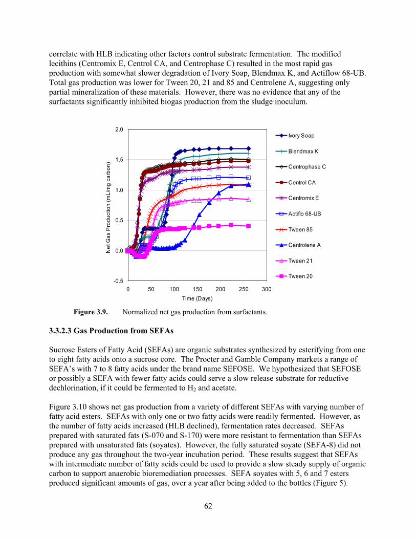
62

correlate with HLB indicating other factors control substrate fermentation. The modified lecithins (Centromix E, Centrol CA, and Centrophase C) resulted in the most rapid gas production with somewhat slower degradation of Ivory Soap, Blendmax K, and Actiflow 68-UB. Total gas production was lower for Tween 20, 21 and 85 and Centrolene A, suggesting only partial mineralization of these materials. However, there was no evidence that any of the surfactants significantly inhibited biogas production from the sludge inoculum.

-0.5

0.0

0.5

1.0

1.5

2.0

0 50 100 150 200 250 300Time (Days)

Net

Gas

Pro

duct

ion

(mL/

mg

carb

on)

Ivory Soap

Blendmax K

Centrophase C

Centrol CA

Centromix E

Actiflo 68-UB

Tween 85

Centrolene A

Tween 21

Tween 20

Figure 3.9. Normalized net gas production from surfactants.

3.3.2.3 Gas Production from SEFAs Sucrose Esters of Fatty Acid (SEFAs) are organic substrates synthesized by esterifying from one to eight fatty acids onto a sucrose core. The Procter and Gamble Company markets a range of SEFA’s with 7 to 8 fatty acids under the brand name SEFOSE. We hypothesized that SEFOSE or possibly a SEFA with fewer fatty acids could serve a slow release substrate for reductive dechlorination, if it could be fermented to H2 and acetate. Figure 3.10 shows net gas production from a variety of different SEFAs with varying number of fatty acid esters. SEFAs with only one or two fatty acids were readily fermented. However, as the number of fatty acids increased (HLB declined), fermentation rates decreased. SEFAs prepared with saturated fats (S-070 and S-170) were more resistant to fermentation than SEFAs prepared with unsaturated fats (soyates). However, the fully saturated soyate (SEFA-8) did not produce any gas throughout the two-year incubation period. These results suggest that SEFAs with intermediate number of fatty acids could be used to provide a slow steady supply of organic carbon to support anaerobic bioremediation processes. SEFA soyates with 5, 6 and 7 esters produced significant amounts of gas, over a year after being added to the bottles (Figure 5).

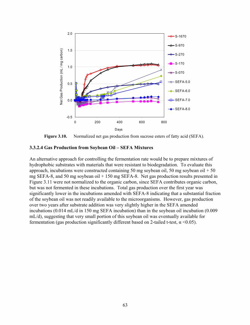
63

-0.5

0.0

0.5

1.0

1.5

2.0

0 200 400 600 800

Days

Net

Gas

Pro

duct

ion

(mL

/ mg

carb

on)

S-1670

S-970

S-270

S-170

S-070

SEFA-5.0

SEFA-6.0

SEFA-7.0

SEFA-8.0

Figure 3.10. Normalized net gas production from sucrose esters of fatty acid (SEFA).

3.3.2.4 Gas Production from Soybean Oil – SEFA Mixtures An alternative approach for controlling the fermentation rate would be to prepare mixtures of hydrophobic substrates with materials that were resistant to biodegradation. To evaluate this approach, incubations were constructed containing 50 mg soybean oil, 50 mg soybean oil + 50 mg SEFA-8, and 50 mg soybean oil + 150 mg SEFA-8. Net gas production results presented in Figure 3.11 were not normalized to the organic carbon, since SEFA contributes organic carbon, but was not fermented in these incubations. Total gas production over the first year was significantly lower in the incubations amended with SEFA-8 indicating that a substantial fraction of the soybean oil was not readily available to the microorganisms. However, gas production over two years after substrate addition was very slightly higher in the SEFA amended incubations (0.014 mL/d in 150 mg SEFA incubation) than in the soybean oil incubation (0.009 mL/d), suggesting that very small portion of this soybean oil was eventually available for fermentation (gas production significantly different based on 2-tailed t-test, α <0.05).

64

0

25

50

75

0 200 400 600 800

Days

Net

Gas

Pro

duct

ion

(mL)

50 mg Soybean Oil50 mg Soybean Oil + 50 mg SEFA-850 mg Soybean Oil + 150 mg SEFA-8

Figure 3.11. Effect of mixing fermentable and non-fermentable substrates on gas production.

3.3.3 PCE Biodegradation in Intermittent Flow Columns Based on the results obtained in the batch incubations, intermittent flow column experiments were conducted over a 14 month period to evaluate the ability of emulsified liquid soybean oil and S-270 SEFA to support reductive dechlorination without excessive methane production and to evaluate the effect of varying sulfate levels on pollutant degradation. The columns were operated with an average hydraulic retention time of ~ 4 days to ensure that an excess of PCE would be present throughout the columns. Columns were initially bioaugmented with a dechlorinating enrichment culture or dechlorinating enrichment culture plus anaerobic digester sludge to evaluate the effect of the initial microbial population on substrate life. Dissolved oxygen was depleted in all of the live, substrate amended columns throughout the duration of the experiment (data not shown). PCE was not significantly depleted in any of the columns due to the short hydraulic retention time (~ 4 days), high PCE loading (over 5 mg/L), and slowly biodegradable substrates. However, both soybean oil and S-270 did enhance sulfate reduction, methanogenesis and cis-DCE production. The cis-DCE production rate increased gradually, reaching a maximum at the end of the project, indicating the added substrates had not yet been depleted over 14 months of operation. VC and ethene production was negligible throughout the duration of the experiment. Figure 3.12 shows the average sulfate removal observed in the sulfate amended columns treated with soybean oil, S-270, and no added carbon. Extensive sulfate removal was observed in the soybean oil amended columns. Sulfate reduction began shortly after column start up with significant sulfate removal observed at the one month sampling event. Some sulfate removal was also observed in the S-270 amended columns; however, sulfate reduction was more limited than in the soybean oil columns. Soybean oil addition also resulted in substantially greater methane production than S-270 addition in the live and live + sludge columns (Figure 3.13). Methanogenesis was completely inhibited in the S-270 / live + SO4 columns by competition with sulfate reducers for the limited H2 and acetate supply.

65

0

500

1000

1500

2000

Influent No Carbon S-270 Soy Oil

Tota

l Sul

fate

(mg)

Figure 3.12. Total mass of sulfate entering (influent) and discharging from sulfate amended

columns. Error bars are experimental range.

0

0.2

0.4

0.6

0.8

1

1.2

1.4

InhibitedControl

Live Live + SO4 Live + Sludge

CH

4 Pr

oduc

ed (m

g/L) No Carbon

S-270Soy Oil

Figure 3.13. Effect of substrate, sulfate and digester sludge addition on CH4 production. Error

bars are experimental range in duplicate columns. Average concentrations of cis-DCE in the column effluents are shown in Figure 3.14. Typically, very little TCE, VC and ethene were detected in the column effluents (data not shown). In all live treatments (live, live + SO4, live + sludge), soybean oil addition resulted in most extensive conversion of PCE to cis-DCE, followed by S-270 and the no added substrate control. Some cis-DCE production was also observed in the no substrate controls due to the bioaugmentation culture / digester sludge added to these columns.

66

0.1

1

10

100

InhibitedControl

Live Live + SO4 Live + Sludge

cis-

DC

E Pr

oduc

ed (m

g/L)

No CarbonS-270Soy Oil

Figure 3.14. Effect of substrate, sulfate and digester sludge addition on cis-DCE production.

Error bars are experimental range in duplicate columns. These results demonstrate that emulsified soybean oil and SEFA S-270 can support sulfate reduction, methanogenesis and reductive dechlorination of PCE to cis-DCE. When high removal rates are required (high PCE and SO4 levels, short HRT), soybean oil would be a more appropriate substrate. However, when slower degradation rates are acceptable, a SEFA or similar slowly biodegradable substrate could be used to reduce the frequency of substrate addition. 3.3.4 Implication for Field Application of Slow Release Substrates The rate and extent of CO2 / CH4 evolution varied widely between the different materials with a few substrates did support methane production for extended time periods. The biogas production rate decreased with increasing number of fatty acid esters and was lower for SEFAs prepared with saturated fats (solids) than unsaturated fats (liquids) suggesting that these materials could be designed to produce H2 and acetate at a controlled rate over extended time periods. This conclusion was supported by column studies where rates of sulfate consumption and contaminant biodegradation could be controlled by using different organic substrates. However, reductive dechlorination of PCE to cis-DCE was also reduced. This suggests that biobarriers constructed with slow release substrates may need to have a greater hydraulic retention time to achieve required treatment efficiencies. Additional research will be required to determine slow release substrates can be used to control substrate lifetime and required reinjection frequency in the field.

67

3.4 REFERENCES AFCEE and NFESC. 2004. Principles and Practices of Enhanced Anaerobic Bioremediation of

Chlorinated Solvents, Air Force Center for Environmental Excellence, Brooks Air Force Base, Texas and Naval Facilities Engineering Service Center (NFESC), Port Hueneme, CA.

Adamson, D.T., McDade, J.M., Hughes, J.B., 2003. Inoculation of DNAPL source zone to

initiate reductive dechlorination of PCE. Environ. Sci. Technol., Vol. 37, No. 11, pp. 2525-2533.

ARCADIS Geraghty & Miller, Inc. (ARCADIS), 2002. Technical Protocol for Using Soluble

Carbohydrates to Enhance Reductive Rechlorination of Chlorinated Aliphatic Hydrocarbons, Prepared for the Air Force Center for Environmental Excellence, San Antonio, Texas and the Environmental Security Technology Certification Program, Arlington, Virginia.

Ballapragada, B.S., Stensel, H.D., Puhakka, J.A., Ferguson, J.F., 1997. Effect of hydrogen on

reductive dechlorination of chlorinated ethenes. Environ. Sci. Technol. Vol. 31, No. 6, pp 1728-34.

Bengtsson, G., Annadotter, H, 1989. Nitrate reduction in a groundwater microcosm determined

by 15N gas chromatography-mass spectrometry. Appl Environ Microbiol. Vol. 55, No. 11, pp. 2861–2870.

Bradley P.M., 2003. History and ecology of chloroethene biodegradation: A review,

Bioremediation J., 7(2): 81-109. Buswell, A.M., Hatfield, W.D. (eds.), 1936. Anaerobic Fermentations, State of Illinois, Dept. of

Registration and Education, Div. of the State Water Survey, Urbana, IL, Bull. No. 32, 1-193.

Colleran, E., Concannon, F., Golden, T., Geoghengan, F., Crumlish, B., Killilea, E., Henry, M.,

Coates, J., 1992. Use of methanogenic activity tests to characterize anaerobic sludges, screen for anaerobic biodegradability, and determine toxicity thresholds against individual trophic groups and species. Water Sci. Technol. Vol. 25, pp. 31-40.

Cooper, D.C., Picardal, F., Rivera, J., Talbot, C., 2000. Zinc immobilization and magnetite

formation via ferric oxide reduction by Shewanella putrefaciens 200. Environ. Sci. Technol. Vol. 34, pp. 100-106.

Coulibaly, K.M., and Borden, R.C., 2004. Impact of edible oil injection on the permeability of

aquifer sands, J. Cont. Hydrol., 71, 219– 237.

68

Coulibaly, K.M., Long, C.M., and Borden, R.C., 2006. Transport of Edible Oil Emulsions in Clayey-Sands: 1-D Column Results and Model Development, J. Engr. Hydrology, 11(3):230-237.

De Bruin, W.P., Kotterman, M.J., Posthumus, M.A., Schraa, G., Zehnder, A.J., 1992. Complete

biological reductive transformation of tetrachloroethene to ethane. Appl. Environ. Microbiol. Vol. 58, No. 6, pp. 1996-00.

DiStefano, T.D., Gossett, J.M., Zinder, S.H., 1991. Reductive dehalogenation of high

concentrations of tetrachloroethene to ethane by an anaerobic enrichment culture in the absence of methanogenesis. Appl. Environ. Microbiol. Vol 57, No.8, pp.2787-92.

Dybas, M.J., Tatara, G.M., Witt, M.E., Criddle, C.S. Slow-release substrates for transformation

of carbon tetrachloride by Pseudomonas strain KC., 1997. In In Situ and On Site Bioremediation: Vol. 3. Papers from the 4th Int. In Situ and On Site Bioremediation Sym. New Orleans, LA. pp. 59. Columbus: Battelle Press.

Earth Tech., 2001. In situ reductive treatment of groundwater contaminated with explosives and

nitrate using HRC®. Technical Bulletin. Ellis, D.E., Lutz, E.J., Odom, J.M., Buchanan, R.J., Bartlett, C.L., Lee, M.D., Harkness, M.R.,

Deweerd, K.A., 2000. Bioaugmentation for accelerated in situ anaerobic bioremediation. Environ. Sci. Technol. Vol. 34, pp. 2254-2260.

Federal Remediation Technology Roundtable (FRTR), 2004. Cost and Performance Summary

Report - Enhanced In Situ Reductive Dechlorination of Trichloroethene Using Edible Oil Emulsion, Altus Air Force Base, Oklahoma, http://www.frtr.gov/costperf.htm.

Freedman, D.L., Gossett, J.M., 1989. Biological reductive dechlorination of tetrachloroethylene and

trichloroethylene to ethylene under methanogenic conditions. Appl. Environ. Microbiol. Vol 55, No. 9, pp. 2144-2151.

Haas, P.E., Cork, P., Aziz, C.E., and Hampton, M., 2000. In situ biowall containing organic mulch

promotes chlorinated solvent bioremediation. In Proc. 2nd. Internat. Conf. Remediation Chlorinated and Recalcitrant Compounds, Monterey, CA, Vol. 4, pp. 71-76.

Hanaki, Matsuo, K.T., Nagase, M., 1981. Mechanism of inhibition caused by long-chain fatty acids

in anaerobic digester process. Biotech. Bioeng. Vol. 23, pp. 1591. He, J.Z., Sung, Y., Dollhopf, M.E., Fathepure, B.Z., Tiedje, J.M., Loffler, F.E., 2002. Acetate

versus hydrogen as direct electron donors to stimulate the microbial reductive dechlorination process at chloroethene-contaminated sites. Environ. Sci. Technol., Vol. 36, No. 18, pp. 3945-3952.

Hunter, W.J., 2001. Use of vegetable oil in a pilot-scale denitrifying barrier. J. Cont. Hydro. Vol.

53, pp. 119-131.

69

Hunter, W.J., 2002. Bioremediation of chlorate or perchlorate contaminated water using

permeable barriers containing vegetable oil. Current Microbiol., 45, 287-292. Kenealy, W., Zeikus, J.G., 1981. Influence of corrinoid antagonists on methanogen metabolism.’

J. Bacteriol., 146, 133–140. Lalman, J.A., and Bagley, D.M., 2001. Anaerobic degradation and methanogenic inhibitory

effects of oleic and stearic acids. Water Resources, Vol. 35, No. 12, pp. 2975-2983. Lee, M.D., Quinton, G.E., Beeman, R.E., Biehle, A.A., Liddle, R.L., 1997. Scale-up issues for in situ

anaerobic tetrachloroethene bioremediation. J. Ind. Microbiol. Biotechnol. Vol. 18, pp. 106-15.

Lee, I.S., Bae, J.H., Yang, Y., McCarty, P.L., 2004. Simulated and experimental evaluation of

factors affecting the rate and extent of reductive dehalogenation of chloroethenes with glucose, J. Cont. Hydrol. 74: 313-331.

Logan, B., 2001. Assessing the outlook for perchlorate remediation. Environ Sci. Technol. Vol.

35, pp. 418-487. Long, C.M., 2004. Enhanced Reductive Dechlorination in Edible oil barriers – experimental and

modeling results, Master of Science Thesis, North Carolina State University, Raleigh, NC.

Koster, I. W., and A. Cramer, 1987. Inhibition of methanogenesis from acetate in granular sludge

by long-chain fatty acids, Appl. Environ. Microbiol. Vol. 53, No. 2, 403-409. Maymo-Gatell, X., Chien, Y., Gossett, J.M., and Zinder, S.H., 1997. Isolation of a bacterium that

reductively dechlorinates tetrachloroethene to ethene, Science, 276: 1568-1571. Pfeiffer, P., 2003. Abiotic Effects of Vegetable Oil Added to Enhance In-Situ Bioremediation of

Chlorinated Solvents. Masters of Science Thesis, University of Colorado, Boulder, CO. Regenesis., 2003. Chromium remediation in groundwater. HRC Technical Bulletin. 2.7.5. Rodin, E., 2001. Influence of Microbial Iron and Nitrate Reduction on Subsurface Iron

Biogeochemistry and Contaminant Metal Mobilization. University of Alabama. Sewell, G.W., Gibson, S.A., 1991. Stimulation of the reductive dechlorination of tetrachloroethene

in anaerobic aquifer microcosms by the addition of toluene. Environ. Sci. Technol. Vol. 25, pp. 982-984.

Shelton, D.R., Tiedje, J.M., 1984a. General method for determining anaerobic biodegradation

potential. Appl. Environ. Microbiol. Vol. 47, No. 4, pp. 850-857.

70

Shelton, D.R. and Tiedje, J.M., 1984b. Isolation and partial characterization of bacteria in an anaerobic consortium than mineralizes 3-chlorobenzoic acid. Appl. Environ. Microbiol. Vol. 45, pp. 840-848.

Smatlak, C., Gossett, J.M., Zinder, S.H., 1996. Comparative kinetics of hydrogen utilization for

reductive dechlorination of tetrachloroethene and methanogenesis in an anaerobic enrichment culture. Environ. Sci. Technol. Vol. 30, No. 9, pp. 2850-58.

Solutions-IES, 2006. Draft Protocol for Enhanced In Situ Bioremediation Using Emulsified

Edible Oil, Environmental Technology Certification Program (ESTCP), Arlington, VA, pp. 1 – 99.

Sorenson, K.S., Martin, J.P., Brennan, R.A., Werth, C.J., Sanford, R.A., and Bures, G.H., 2002.

Phase I SBIR Final Report: Development of a Chitin-Fracing Technology for Remediation of Chlorinated Solvent Source Areas in Low Permeability Media. North Wind Environmental, NWE-ID-2002-024.

Straub, K.L., Benz, M., Schink, B., Widdel, F., 1996. Anaerobic, nitrate-dependent microbial

oxidation of ferrous iron. Appl. Environ. Microbiol. Vol. 62, pp. 1458-1460. Suflita, J., Concannon, F., 1995. Screening tests for assessing the anaerobic biodegradation of

pollutant chemicals in subsurface environments. J. Microbiol. Methods Vol 21, pp. 267-281.

Sung, Y., Ritalahti, K.M., Sanford, R.A., Urbance, J.W., Flynn, S.J., Tiedje, J.M., Loffler, F.E.,

2003. Characterization of two tetrachloroethene-reducing, acetate-oxidizing anaerobic bacteria and their description as Desulfuromonas michiganensis sp nov. App. Environ. Microbiol. Vol. 69, No. 5, pp. 2964-2974.

Vogel, T.M., McCarty, P.L., 1985. Biotransformation of tetrachloroethylene to trichloroethylene,

dichloroethylene, vinyl chloride, and carbon dioxide under methanogenic conditions. Appl. Environ. Microbiol. Vol. 49, No. 5, pp. 1080-83.

Weber, K.A., Picardal, F., Roden, E., 2001. Microbially-catalyzed nitrate-dependent oxidation of

biogenic solid-phase Fe(II) compounds. Environ. Sci. Technol. Vol. 35, pp. 1644-1650. Werth, C., Sanford, R., 2002. A passive in-situ bioremediation technology for chlorinated

solvents. Illinois Groundwater Association. Spring meeting 2002. Wolin, E.A., Wolin, M.J., Wolfe, R.S. 1963. ‘Formation of methane by bacterial extracts.’ J.

Biol. Chem., 238, 2882–2886. Zawtocki, C., Lieberman, M.T., Borden, R.C., and Birk, G.M., 2004. Treatment of perchlorate

and 1,1,1-trichloroethane in groundwater using edible oil substrate (EOS®), Proceedings of Remediation of Chlorinated and Recalcitrant Compounds – 4th Internat. Conf., Monterey, CA.

71

Zenker, M. J., R. C. Borden, M. A. Barlaz, M. T. Lieberman, and M. D. Lee. 2000. "Insoluble

Substrates for Reductive Dehalogenation in Permeable Reactive Barriers." In G. B. Wickranayake, A. R. Gavaskar, B. C. Alleman, and V. S. Magar (Eds.), Bioremediation and Phytoremediation of Chlorinated and Recalcitrant Compounds. pp 77 - 84. Battelle Press. Columbus, OH.

72

CHAPTER 4: TRANSPORT AND RETENTION OF EDIBLE OIL EMULSIONS IN AQUIFER MATERIALS

4.1 INTRODUCTION In-situ anaerobic bioremediation processes are being implemented for treatment of a wide variety of groundwater contaminants including chlorinated solvents, nitrate, perchlorate and acid mine drainage (Morse et al. 1998, Hunter 2001, Hunter 2002, AFCEE 2004, ITRC 2002). In all of these processes, one or more biodegradable organic substrates are distributed throughout the treatment zone to provide a carbon source for cell growth and an electron donor for energy generation. There has been considerable interest in using soybean oil as a substrate for in-situ bioremediation because of its’ low cost, food-grade status, and longevity in the subsurface. However, injection of soybean oil into the subsurface as a neat liquid may be difficult because of the limited spread of the oil and large amount of chase water required to displace the oil to residual saturation (Zenker et al. 2000, Lee et al. 2001, Casey et al. 2002). To overcome these problems, Coulibaly and Borden (2004) developed a process for distribution of soybean oil as an oil-in-water emulsion consisting of small oil droplets dispersed in a continuous water phase. The emulsion was prepared to: (1) be stable for extended time periods (e.g. non-coalescing); (2) have small, uniform droplets to allow transport in most aquifers; and (3) have a negative surface charge to reduce droplet capture by the solid surfaces. The emulsion would be distributed throughout the proposed treatment zone by injecting a dilute emulsion followed by one or more pore volumes (PV) of water to distribute and immobilize the oil droplets. Since water is the continuous phase, oil-in-water emulsions are completely miscible with water and can be injected as any other aqueous solution. While the available laboratory and field data indicate that emulsions can be effectively distributed in typical aquifer materials, some questions remain.

• There is limited information on the transport and distribution of edible oil emulsions in different aquifer materials.

• There are no generally recognized tools for predicting the effect of injection

conditions on the resulting oil distribution. • Edible oils are less dense than water so there is potential for buoyancy effects that

could result in poor oil distribution in deeper portions of the aquifer where contaminant concentrations may be high.

• In-situ treatments are often complicated to implement because of difficulties

associated with distributing treatment agents throughout heterogeneous aquifers.

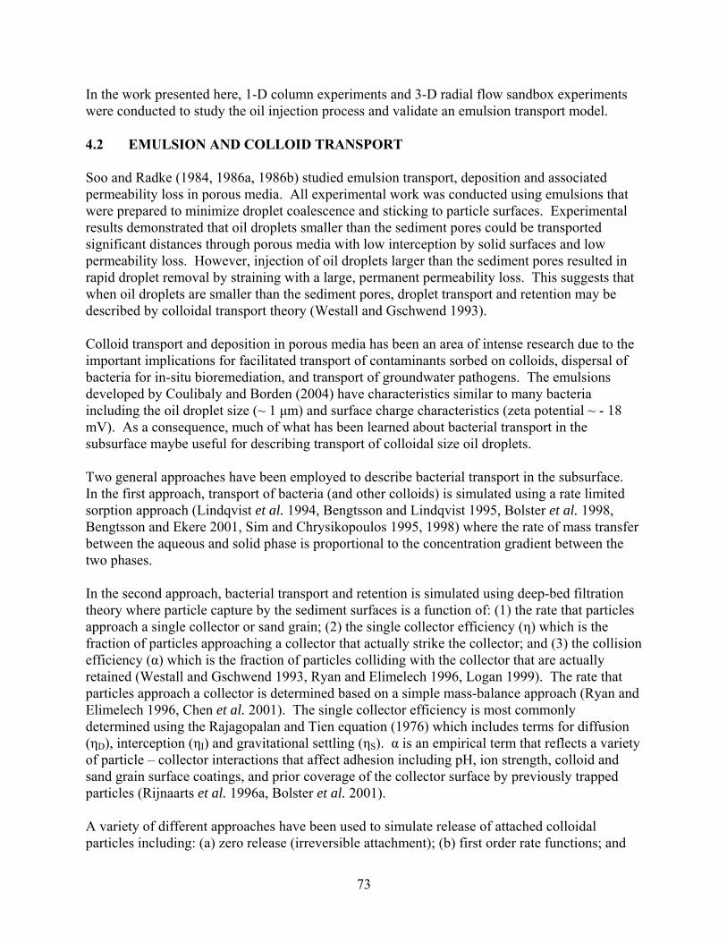
73

In the work presented here, 1-D column experiments and 3-D radial flow sandbox experiments were conducted to study the oil injection process and validate an emulsion transport model. 4.2 EMULSION AND COLLOID TRANSPORT Soo and Radke (1984, 1986a, 1986b) studied emulsion transport, deposition and associated permeability loss in porous media. All experimental work was conducted using emulsions that were prepared to minimize droplet coalescence and sticking to particle surfaces. Experimental results demonstrated that oil droplets smaller than the sediment pores could be transported significant distances through porous media with low interception by solid surfaces and low permeability loss. However, injection of oil droplets larger than the sediment pores resulted in rapid droplet removal by straining with a large, permanent permeability loss. This suggests that when oil droplets are smaller than the sediment pores, droplet transport and retention may be described by colloidal transport theory (Westall and Gschwend 1993). Colloid transport and deposition in porous media has been an area of intense research due to the important implications for facilitated transport of contaminants sorbed on colloids, dispersal of bacteria for in-situ bioremediation, and transport of groundwater pathogens. The emulsions developed by Coulibaly and Borden (2004) have characteristics similar to many bacteria including the oil droplet size (~ 1 μm) and surface charge characteristics (zeta potential ~ - 18 mV). As a consequence, much of what has been learned about bacterial transport in the subsurface maybe useful for describing transport of colloidal size oil droplets. Two general approaches have been employed to describe bacterial transport in the subsurface. In the first approach, transport of bacteria (and other colloids) is simulated using a rate limited sorption approach (Lindqvist et al. 1994, Bengtsson and Lindqvist 1995, Bolster et al. 1998, Bengtsson and Ekere 2001, Sim and Chrysikopoulos 1995, 1998) where the rate of mass transfer between the aqueous and solid phase is proportional to the concentration gradient between the two phases. In the second approach, bacterial transport and retention is simulated using deep-bed filtration theory where particle capture by the sediment surfaces is a function of: (1) the rate that particles approach a single collector or sand grain; (2) the single collector efficiency (η) which is the fraction of particles approaching a collector that actually strike the collector; and (3) the collision efficiency (α) which is the fraction of particles colliding with the collector that are actually retained (Westall and Gschwend 1993, Ryan and Elimelech 1996, Logan 1999). The rate that particles approach a collector is determined based on a simple mass-balance approach (Ryan and Elimelech 1996, Chen et al. 2001). The single collector efficiency is most commonly determined using the Rajagopalan and Tien equation (1976) which includes terms for diffusion (ηD), interception (ηI) and gravitational settling (ηS). α is an empirical term that reflects a variety of particle – collector interactions that affect adhesion including pH, ion strength, colloid and sand grain surface coatings, and prior coverage of the collector surface by previously trapped particles (Rijnaarts et al. 1996a, Bolster et al. 2001). A variety of different approaches have been used to simulate release of attached colloidal particles including: (a) zero release (irreversible attachment); (b) first order rate functions; and

74

(c) retention time dependent approaches. In the retention time dependent approach, the probability of colloid release from the sediment surface decreases with time that the particle is attached (Meinders et al. 1992, 1995, Johnson et al. 1995, Becker et al. 2004). The increasing strength of particle attachment with time is thought to be associated with gradual displacement of a thin water layer separating the colloid from the collector surface. In this work, we evaluate the use of a deep-bed filtration approach for simulating emulsion transport in 1-D laboratory columns and 3-D radial flow sandboxes. 4.3 EMULSION TRANSPORT IN 1-D LABORATORY COLUMNS The transport and retention of oil-in-water emulsions may be simulated using the standard advection-dispersion equations with terms representing colloid capture by the sand grain surfaces and droplet release back to the mobile phase where (Bolster et al. 1998, Camesano et al. 1999).

( ) RCKvCxx

CDxt

C Bmam

mm

0ερ

+−∂∂

−⎟⎠⎞

⎜⎝⎛

∂∂

∂∂

=∂∂

(1)

and

RCKt

Cm

Ba

im −=∂∂

ρε0

(2)

where Cm = mobile phase concentration (ML-3) Cim = immobile phase concentration (M M-1) t = time (T) x = distance (L) D = dispersion coefficient (L2T-1) v = pore water velocity (LT-1) Ka = attachment rate (T-1) ρB = bulk density (ML-3) ε0 = porosity (dimensionless) R = immobile phase release rate (T-1) For an empty bed, the attachment rate, Ka, can be calculated as

αηε⎟⎟⎠

⎞⎜⎜⎝

⎛ −=

ca d

vK 0123

(3)

75

α = collision efficiency (dimensionless) η = single collector efficiency (dimensionless) dc = equivalent collector diameter (L) Extensive work over the past decade has shown that a variety of factors influence collision efficiency including geochemical conditions, double layer thickness, surface roughness, shadow effects, sediment surface charge heterogeneity, and blocking of the sediment surface with previously retained colloids (Johnson and Elimelech 1995, Rijnaarts et al. 1996b, Camesano et al. 1999, Ko et al. 2000, Ko and Elimelech 2000). In well controlled laboratory systems, these different factors can be isolated and modeled using well defined, physically based parameters. However, it may not be practical to model these separate processes when emulsions with a range of droplet sizes are injected into natural aquifers with a varying grain sizes and geochemical characteristics. Under these conditions, it may be more useful to represent collision efficiency using a simplified Langmuirian blocking relationship of the form maxmax /)(' imimim CCC −=αα where max

imC is an empirical measure of the maximum mass of particles captured per mass sediment. Substituting this relationship for α in equation 3 we obtain:

ηαε⎟⎟⎠

⎞⎜⎜⎝

⎛ −⎟⎟⎠

⎞⎜⎜⎝

⎛ −= max

max0 '1

23

im

imim

ca C

CCd

vK (4)

The mechanisms controlling release of attached colloids are poorly understood. Many previous investigators have assumed colloid release to be negligible (i.e., R = 0, Bolster et al. 1998) or attachment to be irreversible (Johnson and Elimelech 1995, Johnson et al. 1996). In this work, oil droplet release was observed to be very limited and R was assumed to be zero. 4.3.1 Materials and Methods All experiments were conducted with a medium to fine sand amended with 0%, 2.5% or 5% kaolinite (Thiele Kaolin Company, Sandersville, Georgia). The original material termed Field Sand (FS-7%) was obtained from a local supplier (Caudle Sand and Rock, Raleigh, NC) and used in prior studies by Coulibaly and Borden (2004). Characteristics of each material are summarized in Table 4.1. The -_% designation is used to indicate the weight fraction finer than 75 µm (silt + clay fraction). Kaolinite addition had little effect on the median grain diameter (D50) but increased the D60/D10 ratio by an order of magnitude.

Table 4.1 Characteristics of Sediments Used in Column Experiments.

Material D50 (mm)

D10 (mm) D60 / D10

% Finer than 75 μm(#200 sieve)

Field Sand (FS-7%) 0.38 0.10 4.5 6.9 Field Sand + 2.5% kaolinite (FS-9%) 0.36 0.074 6.0 9.2

Field Sand + 5% kaolinite (FS-12%) 0.37 0.0067 67 11.5

76

Coulibaly and Borden (2004) demonstrated that oil-in-water emulsions with small, uniform droplets can be prepared using soybean oil and food grade surfactants. The emulsions used in this work were prepared by blending 33% by volume soybean oil, 62% tap water and 5% premixed surfactant (38% polysorbate 80, 56% glycerol monooleate (GMO) from Lambent Technologies and 6% water) in a Waring Commercial blender at high speed for 5 minutes. The mean droplet size was 1.2 µm (standard dev. = 1.3 µm). The zeta potential of the oil droplets, sand, and kaolinite in tap water (pH= 8.2, specific conductance = 190 µS/cm) were -18, -22 and -24 mV indicating unfavorable conditions for the negatively charged oil droplets to stick to the negatively charged sand and kaolinite collectors (Coulibaly and Borden 2004). Emulsion transport and retention was examined in 80 cm long by 2.9 cm (~1 inch) polyvinyl chloride (PVC) columns. The columns were dry packed with sediment while constantly tapping to induce settlement. After evacuating the columns, deaired tap water was slowly introduced into the column inlet to minimize entrapped air. Deaired water was then pumped upward through the columns at ~ 2.5 mL/min for 2 hours to further saturate the columns. The emulsion injection test consisted of pumping 25 mL of 11% oil by volume emulsion (~0.05 PV of pure oil) followed by 1000 mL (~5PV) of deaired tap water. The effluent was collected every 30 mL and analyzed for oil content by volatile solids (VS) analysis. VS were determined by weight loss on ignition for 1 hour at 550 ºC (standard deviation of replicates typically less than 5% of mean). After completion of the experiment, the column was frozen, cut into 8 sections of 10 cm each, with each section analyzed for oil content by VS analysis. Because of the filters used at each end of the column, the oil concentration in the first and the last segment were less reliable. Prior to emulsion injection, non-reactive tracer tests were conducted by pumping 25 mL of 175 mg/l NaBr solution through each column at a flow rate of ~2.5 mL/min followed by 1000 mL of deaired water. Effluent samples were analyzed for Br by ion chromatography. 4.3.2 Experimental Results - Emulsion Transport in Columns Experimental conditions and mass balance results for each of the column experiments are summarized in Table 4.2. Porosity and dispersivity were obtained by fitting a solute transport model to the non-reactive tracer test results. FS-7%-#1, #2 and #3 were conducted at the same injection flowrate (2.25 to 2.38 mL/min). However differences in the sediment porosity resulted in some variability in the solute transport velocity (Table 2). FS-7%-slow was conducted with a lower injection rate (0.5 mL/min) to evaluate the effect of transport velocity on oil retention. FS-9% and FS-12% examined the effect of increasing clay content on oil retention. Overall mass balances for most experiments were reasonable with the exception of FS-7%-#3 where only 65% of the injected mass was recovered in the column effluent and the sediment at the end of the experiment. The high mass balance error may be related to difficulties in correcting for the background volatile solids content of the sediment.

77

Table 4.2 Emulsion Transport Parameters and Mass Balance Results

Oil released (%) Material Bulk Density (g/cm3)

Porosity (mL/cm3)

Dispersivity (cm)

Velocity (m/d)

α’ maximC

(mg/g) Mass

balance (%) Experimental Model

FS-7%-#1 1.82 0.31 2.0 15.5 0.021 5.4 93 12.10 7.45 FS-7%-#2 1.44 0.46 8.0 11.1 0.073 5.4 105 6.50 4.12 FS-7%-#3 1.52 0.43 8.4 12.1 0.064 5.4 65 4.35 3.78 FS-7%-slow 1.66 0.37 3.0 2.9 0.036 5.4 87 1.23 0.75

FS-9% 1.73 0.35 0.4 18.4 0.030 6.1 106 0.51 0.06 FS-12% 1.74 0.34 1.0 18.6 7.67 x 10-5 9.5 116 0.01 0.08

78

Experimental results for the three replicate FS-7% injection experiments and single low velocity FS-7% experiment are shown in Figure 4.1. Oil released in the column effluent varied from 4 to 12 % of the injected mass. In all four experiments, peak effluent emulsion concentrations were observed at approximately one pore volume indicating no significant enhancement or retardation of the oil droplets. The maximum emulsion concentrations in the effluent of the three fast columns were 2.55, 0.66 and 0.7 g/L or 0.6 to 2.4% of the injection concentration. By contrast, the maximum non-reactive tracer concentrations were 13 to 27 % of the injection concentration (data not shown). After roughly 300 minutes, the turbidity of the column effluents declined (based on visual observation) and the VS concentrations reached a steady-state value of 0.01 – 0.10 g/L (detection limit = 0.01 g/L). The low effluent turbidity suggests that most of the VS released at the end of the experiments was dissolved, not colloidal oil droplets. However, it was not possible to distinguish between colloid size oil droplets and dissolved organic material (oil, surfactant, or biotransformation products) using the VS analytical method, so some oil droplets may have been released.

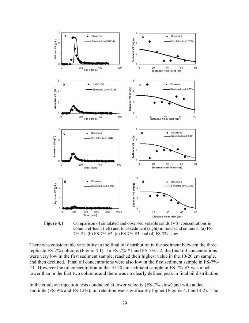
79

0

1

2

3

0 200 400 600Tim e (m in)

Aqu

eous

VS

(g/L

)

Observed

Simulated (α=0.0733)

b

0

1

2

3

0 200 400 600Tim e (m in)

Aqu

eous

VS

(g/L

)

Observed


c

0

1

2

3

0 200 400 600Tim e (m in)

Efflu

ent V

S (g

/L)

Observed


a

0

1

2

3

0 500 1000 1500 2000 2500Tim e (m in)

Aqu

eous

VS

(g/L

)

Observed

Simulated (α=0.0356)d

0

3

6

9

0 20 40 60 80Distance from inlet (cm )

Sedi

men

t VS

(mg/

g)

Observed


a

0

3

6

9

0 20 40 60 80Distance from inlet (cm )

Sedi

men

t VS

(mg/

g)

Observed


b

0

3

6

9

0 20 40 60 80Distance from inle t (cm )

Sedi

men

t VS

(mg/

g)ObservedSimulated (α=0.064)

c

0

3

6

9

0 20 40 60 80

Distance from inlet (cm )

Sedi

men

t VS

(mg/

g)

ObservedSimulated (α=0.0356)

d

Figure 4.1 Comparison of simulated and observed volatile solids (VS) concentrations in

column effluent (left) and final sediment (right) in field sand columns: (a) FS-7%-#1; (b) FS-7%-#2; (c) FS-7%-#3; and (d) FS-7%-slow.

There was considerable variability in the final oil distribution in the sediment between the three replicate FS-7% columns (Figure 4.1). In FS-7%-#1 and FS-7%-#2, the final oil concentrations were very low in the first sediment sample, reached their highest value in the 10-20 cm sample, and then declined. Final oil concentrations were also low in the first sediment sample in FS-7%-#3. However the oil concentration in the 10-20 cm sediment sample in FS-7%-#3 was much lower than in the first two columns and there was no clearly defined peak in final oil distribution. In the emulsion injection tests conducted at lower velocity (FS-7%-slow) and with added kaolinite (FS-9% and FS-12%), oil retention was significantly higher (Figures 4.1 and 4.2). The

80

higher oil retention in the FS-7%-slow test is consistent with prior work by Elimelech and Omelia (1990) and Camesano and Logan (1998) who demonstrated that colloid retention is a non-equilibrium process with lower transport velocities leading to increased contact time and greater colloid retention. The transport velocities employed in this work are higher than typically observed under ambient groundwater flow conditions but are comparable to velocities commonly encountered near emulsion injection wells. The trend of increasing oil retention with increasing clay content is consistent with prior results by Coulibaly and Borden (2004).

0

3

6

9

12

15

0 20 40 60 80Distance from inle t (cm )

Sedi

men

t VS

(mg/

g)

Observed

Simulated (α=0.03)a

0

0.05

0.1

0.15

0.2

0.25

0 100 200 300 400Tim e (m in)

Efflu

ent V

S (g

/L)

Observed

Simulated (α=0.03)a

0

3

6

9

12

15

0 20 40 60 80

Distance from inle t (cm )

Sedi

men

t VS

(mg/

g)

Observed

Simulated (α=7.67E-5)b

0

0.05

0.1

0.15

0.2

0.25

0 100 200 300 400

Tim e (m in)

Efflu

ent V

S (g

/L) Observed

Simulated (α=7.67E-5)

b

Figure 4.2 Comparison of simulated and observed volatile solids (VS) concentrations in column effluent (left) and final sediment (right) in columns packed with field sand amended with varying amounts of kaolinite: (a) FS-9%; and (b) FS-12%.

These experimental results show that appreciable amounts of emulsified oils can be transported at least 80 cm from the injection point and will result in a reasonably uniform oil distribution in the experimental columns. However there was significant variability in experimental results between replicate columns. The greater amount of oil released from FS-7%-#1 could be due to the slightly higher transport velocity in this column (Table 4.2). The cause of the observed variability in retained oil distribution is unknown, but may be related to minor variations in packing between columns.

81

4.3.3 Mathematical Model of Emulsion Transport 4.3.3.1 Model development and implementation Emulsion transport was simulated using MODFLOW (MacDonald and Harbaugh 1988) and RT3D (Clement 1997) as implemented in GMS 3.1 (Brigham Young University 1999). Colloid transport is not currently implemented in RT3D, so a user defined module was developed to simulate colloid transport using equations 2, 3, and 4. RT3D uses the operator splitting method to separate the advection part of equation 1 from the reaction part. Changes in Cm and Cim represented by equations 7 and 8 were coded in user-defined module. This module is then compiled as a dynamic link library (dll) that is called by RT3D at runtime.

mim

imima

m CC

CCKt

C⎟⎟⎠

⎞⎜⎜⎝

⎛ −−=

∂∂

max

max

(7)

and

mim

imim

Ba

im CC

CCKt

C⎟⎟⎠

⎞⎜⎜⎝

⎛ −=

∂∂

max

max0

ρε

(8)

where:

ηαε⎟⎟⎠

⎞⎜⎜⎝

⎛ −⎟⎟⎠

⎞⎜⎜⎝

⎛ −= max

max0 '1

23

im

imim

ca C

CCd

vK (9)

The 80 cm columns used in the emulsion transport experiments were represented by a one-dimensional (1-D) grid of 160 cells that were 0.5 cm long by 2.5 cm wide by 2.5 cm high. The column inlet was simulated as an injection well and the outlet was simulated as a drain. Dispersivity and effective porosity were estimated by fitting the RT3D non-reactive tracer module to match bromide tracer results (Table 4.2). Porosity was estimated from the measured bulk density and specific gravity of the sediment. The maximum oil retention capacity ( max

imC ) was assumed equal to the maximum observed oil concentration in the sediment. The equivalent collector diameter (dc) was assumed to be equal to the sediment D10 based on the work of Huber (2000) and Martin et al. (1996) who showed that D10 provided the most representative estimates of collector diameter in well graded sediments. Martin et al. (1996) reported that using D50 or arithmetic averages lead to an underestimation of η resulting in α higher than 1. The single collector efficiency (η) was computed using the Rajagopalan and Tien (1976) relationship

3/23/15/25/68/158/1 400338.0 −− ++= PesRGsRLos NANNANNAη (10)

where:

82

65

5

2332)1(2

γγγγ−+−

−=sA

vdHN

dLo 29

4πμ

=

c

dR d

dN =

vdgN dd

G μρρ

18)( 2−

=

kTdvdN dc

Peπμ3

=

and γ= (1-θ) 1/3

dd and ρd are the equivalent diameter and density of the oil droplets, μ and ρ the viscosity and density of the fluid, T the temperature, H the Hamaker constant, g the gravitational constant and k the Boltzmann constant. Values for the most important parameters used in the computation of η are: equivalent droplet diameter of 1.25 μm, droplet density of 0.95 g/cm3, water viscosity of 9.37 x 10-4 N/sm-2, water density of 1 g/cm3, and temperature of 23 °C. At present, there is no reliable method for independently estimating the empty bed collision efficiency (α’). Consequently, α’ was used as a fitting parameter. When a significant amount of emulsion was released in the column effluent, the best fit value of α’ was found by comparing simulated and observed breakthrough curves (FS-7%-#1, -#2 and -#3). However when less than 2% of injected emulsion was discharged in column effluent, α’ was adjusted to match the observed oil distribution in the sediment (FS-7%-slow, FS-9%, and FS-12%). The best fit value of each parameter was found by the bisection method using the root mean square error as the primary objective function. Model calibration parameters for each of the column experiments are summarized in Table 4.2. 4.3.3.2 Simulation results Model simulation results are compared with observed BTC and the final oil distribution in each field sand column in Figure 4.1. Using α’ as a fitting parameter, the model provides a very good match between simulated and observed BTCs for each of the FS-7% experiments. There was significant variability in the measured final oil distributions, so it was not possible to precisely match the oil distribution in any specific column. However, the model simulates the general trend in the final oil distribution, with higher retention close to the inlet and gradually decreasing

83

concentrations towards the outlet. Figure 4.2 shows a comparison of simulated and observed BTCs and final oil distributions for the FS-9% and FS-12% columns. Over 99% of the oil was retained in the sediment in these two experiments, so the effluent BTC curves are poorly defined. As discussed above, some fraction of the VS released in the column effluent is likely associated with dissolved oil and/or surfactants, not release of colloidal oil droplets. The model provides a good match to the final oil distribution in the FS-9% column. However, the match for the FS-12% column is not nearly as good. The poor match for FS-12% may have been due to experimental issues. The permeability of the FS-12% material was significantly lower than the other sediments which required higher injection pressures to achieve the desired flowrate and could have resulted in flow bypassing around some sections of the column. Overall mass balance results for each of the simulations are compared with experimental results in Table 4.2. Between 88% and 99.9% of the injected oil was retained by the columns with the highest percent retained in for the FS-7% at a low flow rate and for the FS-9% and FS-12% columns. The mathematical model was able to reproduce this general trend very well. Best fit values of the empty bed collision efficiency of oil droplets, α’, in FS-7%, FS-9% and FS-12% were 0.048 (range = 0.021 to 0.073), 0.030 and 0.00007, respectively. The α’ values for FS-7% and FS-9% are similar to values obtained for common bacteria (Camesano and Logan 1998, Camesano et al. 1999, Rijnaarts et al. 1996a). Similarly, the variability α’ is comparable to that observed for bacteria retention by other investigators (Jewett et al. 1995). However, α’ for FS-12% was much lower than FS-7% and FS-9%, indicating the kaolinite is a less efficient collector of oil droplets than the natural clayey sand. 4.4 EMULSION TRANSPORT IN 3-D SAND BOXES 4.4.1 Materials and Methods The experimental setup was designed to simulate one quarter of the flow-field adjoining an emulsion injection point. A plan view of the sandbox and injection well is shown in Figure 4.3. The inside dimensions of the sandbox are 0.98 m wide x 0.98 m deep x 1.2 m high. A double layer of geonet drainage material and single layer of non-woven geotexile fabric were installed along the back and right boundaries. These drainage layers were connected by several different ports to a single reservoir that maintained the back and right sides as constant head boundaries. A 2.5 cm diameter x 100 cm long slotted well screen (#20 slot) was located in the front left corner of the sandbox and connected to a constant head reservoir. With the front and left sides of the tank acting as no-flow boundaries, this setup reasonably represents one quarter of the flow field surrounding an injection point. The 1.0 m injection radius in the laboratory experiment is at a scale comparable to field conditions.

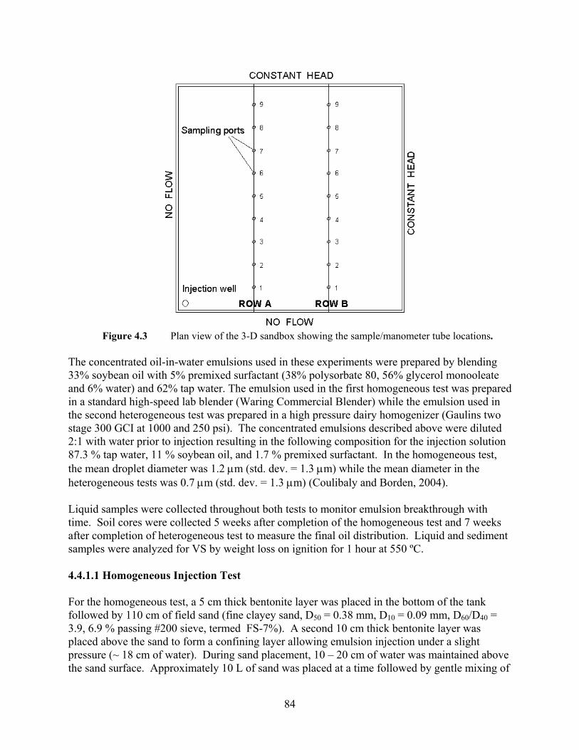
84

Figure 4.3 Plan view of the 3-D sandbox showing the sample/manometer tube locations.

The concentrated oil-in-water emulsions used in these experiments were prepared by blending 33% soybean oil with 5% premixed surfactant (38% polysorbate 80, 56% glycerol monooleate and 6% water) and 62% tap water. The emulsion used in the first homogeneous test was prepared in a standard high-speed lab blender (Waring Commercial Blender) while the emulsion used in the second heterogeneous test was prepared in a high pressure dairy homogenizer (Gaulins two stage 300 GCI at 1000 and 250 psi). The concentrated emulsions described above were diluted 2:1 with water prior to injection resulting in the following composition for the injection solution 87.3 % tap water, 11 % soybean oil, and 1.7 % premixed surfactant. In the homogeneous test, the mean droplet diameter was 1.2 μm (std. dev. = 1.3 μm) while the mean diameter in the heterogeneous tests was 0.7 μm (std. dev. = 1.3 μm) (Coulibaly and Borden, 2004). Liquid samples were collected throughout both tests to monitor emulsion breakthrough with time. Soil cores were collected 5 weeks after completion of the homogeneous test and 7 weeks after completion of heterogeneous test to measure the final oil distribution. Liquid and sediment samples were analyzed for VS by weight loss on ignition for 1 hour at 550 ºC. 4.4.1.1 Homogeneous Injection Test For the homogeneous test, a 5 cm thick bentonite layer was placed in the bottom of the tank followed by 110 cm of field sand (fine clayey sand, D50 = 0.38 mm, D10 = 0.09 mm, D60/D40 = 3.9, 6.9 % passing #200 sieve, termed FS-7%). A second 10 cm thick bentonite layer was placed above the sand to form a confining layer allowing emulsion injection under a slight pressure (~ 18 cm of water). During sand placement, 10 – 20 cm of water was maintained above the sand surface. Approximately 10 L of sand was placed at a time followed by gentle mixing of

85

the sand surface and compaction to remove entrapped air. On a macroscopic scale, this resulted in reasonably uniform packing with little entrapped air. However visual inspection of the sand through the clear acrylic plastic showed some small-scale segregation of sediments where some thin layers appeared to have more clay than others. Two rows (shown as A and B on Figure 1.1) of 2 mm ID stainless steel tubes with nylon screens were installed at 25 cm, 50 cm, and 75 cm from the top of the sand layer for sample collection and to measure changing water levels via a manometer board. Hydrodynamic parameters were estimated using results from a non-reactive tracer test where 60 L (~0.2 PV) of a 200 mg/L NaBr solution was injected followed by 450 L (~1.5 PV) of tap water over a 5 day period. During the emulsion test, 30 L (~ 0.1 PV) of oil-in-water emulsion were injected followed by 450 L of tap water (~1.5 PV) to distribute and immobilize the oil. 4.4.1.2 Heterogeneous Injection Test In the heterogeneous test, a 5 cm bentonite layer was installed on the bottom of the tank, followed by 23 cm of field sand amended with ~5% kaolinite (FS-12%), 48 cm of field sand (FS-7%), 29 cm of field sand amended with ~2.5% kaolinite (FS-9%) and 20 cm of bentonite to form a confining layer. The field sand – kaolinite mixtures were prepared by blending known weights of field sand and kaolinite (Standard Industrial Mineral Inc. Bishop, CA) in concrete mixer for ~ 15 minutes per batch. The stainless steel sampling tubes were screened at 90 cm, 50 cm, and 20 cm from the bottom of the bentonite layer. In the heterogeneous test, the non-reactive tracer was injected as part of the emulsion. Prior to injection, tap water was flushed through the tank for 2 weeks to establish steady-state conditions. The emulsion injection test consisted of injecting 120 L (~0.5 PV) of emulsion amended with 1000 mg/L NaCl followed by 1000 L (~5.0 PV) of tap water. 4.4.2 Experimental Results 4.4.2.1 Homogeneous Injection Test Prior to the start of emulsion injection, a non-reactive tracer test was run and the spatial variation of head with distance was determined to collect data required for calibration of a groundwater flow and emulsion transport model. During emulsion injection, the flowrate dropped to 0.06 m3

/d from a pre-injection value of 0.13 m3 /d (std. dev. = 0.01). Shortly after the start of the post-emulsion water flush, the flowrate recovered to 0.10 m3 /d and then remained relatively constant for the remainder of the test (ave. flow = 0.11 m3 /d, std. dev. = 0.01). Water levels in the injection well and constant head boundaries were held constant throughout the test, so the decline in flowrate during emulsion injection indicates a temporary reduction in the effective hydraulic conductivity. Most of this reduction appears to be due to the somewhat higher viscosity (µ = 1.44 centipoises) and lower density (ρ = 0.99 g/cm3) of the emulsion compared to that of water (µ = 0.95 centipoises, ρ = 1 g/cm3). The recovery in injection flowrate during the post-emulsion water flush indicates that there was no significant, long-term permeability loss associated with the emulsion injection. These results are consistent with prior work by Coulibaly and Borden (2004) who showed that flushing 3 PV of a similar emulsion (median droplet diameter = 1.2 µm) followed by 7 PV of water through FS-7% resulted in only 3% reduction in hydraulic conductivity.

86

Figure 4.4 shows the variation in emulsion concentration versus time in monitoring points at varying distances from the injection well. The maximum concentrations observed in the closest monitoring points were 110%, 37% and 90% of the injection concentration indicating essentially complete emulsion breakthrough at up to 44 cm from the injection well. In the more distant sampling points, emulsion breakthrough was more limited and occurred later in the test as the chase water distributed emulsion throughout the sandbox. In sampling points over 70 cm from the injection well, emulsion concentrations never exceeded 0.5% of the injected concentration. This is in contrast to the non-reactive tracer test results which showed 50% to 100% breakthrough at the same locations and indicates that most of the emulsion was captured by the soil matrix.

0255075

100125

VS

(g/L

)

0255075

100125

Rad. Dis t. = 31 cmRad. Dis t. = 27 cm

00.10.20.30.4

00.10.20.30.4

VS

(g/L

) Rad. Dis t. = 77 cm

0 1 2 3 4

Days

00.10.20.30.4

Rad. Dis t. = 73 cm

0 1 2 3 4

Days

00.10.20.30.4

VS (g

/L) Rad. Dis t. = 106 cmRad. Dis t. = 98 cm

Figure 4.4 Variation in predicted (line) and observed (circles) aqueous volatile solids (VS)

concentration versus time at different radial distance from the injection well for the homogeneous test.

Five weeks after the end of the emulsion injection test, sediment cores were collected from three depths at 9 locations to determine the spatial distribution of residual emulsion in the sediment. During this post-injection period, there was no flow through the tank to evaluate the potential for oil droplets to float upward due to buoyancy effects. Figure 4.5 shows the sediment VS concentration (mg/g) after correcting for the sediment VS prior to injection (5.4 mg/g). The VS results show that emulsion was effectively distributed throughout the tank. However there was a statistically significant (t > t95) trend in VS concentration with radial distance at each depth with slightly higher concentrations in samples collected closer to the injection well. There was no significant difference in sediment VS concentrations between the three sampling zones

87

indicating that buoyancy effects were not significant. The lack of apparent buoyancy effects is not surprising given that: (a) essentially all of the oil droplets were immobilized on the sediment surfaces before termination of water injection; and (b) pressure gradients associated with fluid injection greatly exceeded those that could have been generated by fluid density differences when oil droplets where still mobile.

0246

VS

(mg/

g)

0 20 40 60 80 100 120

Radial Distance (cm)

0246

VS (m

g/g)

Depth = 75 cm

02468

VS

(mg/

g) Depth = 25 cm

Depth = 50 cm

t = 3.79 >1.83(t 95)

t = 3.06 >1.83(t 95)

t = 2.36 >1.83(t 95)

Figure 4.5 Volatile solids concentration in sediment samples collected 5 weeks after the end

of homogeneous test (line is linear regression of experimental results). Approximately 67.5% (95% confidence limits = ± 24 %) of the added emulsion was retained by the sediment based on the average VS in the sandbox (mean = 1.85, std. dev. = 1.66, n = 27) and the amount of sediment in the sandbox. Sampling from one of several discharge ports on the constant head boundaries indicated that 2.5% of the emulsion was released in the sandbox effluent with up to 30% of the emulsion unaccounted. However visual observations indicated considerable variability in emulsion concentration between the different constant head discharge ports, suggesting that more emulsion may have been released in the sandbox discharge than the effluent sampling results indicate. 4.4.2.2 Heterogeneous Injection Test Prior to the start of emulsion injection, tap water was run through the tank at a flowrate of 0.6 m3/d for several weeks to establish steady-state conditions. The spatial variation of head with distance was determined for groundwater model calibration. The emulsion injection test consisted of injecting 120 L (~0.5 PV) of emulsion amended with 1000 mg/l NaCl followed by 1000 L (~5.0 PV) of tap water.

88

During the emulsion injection portion of the test (0 to 10 hr), the flowrate dropped from a pre-injection value of 0.6 m3/d (std. dev. = 0.03) to 0.2 – 0.4 m3/d (Figure 4.6a). When the injection solution was switched back to tap water at 10 hr, the injection flowrate recovered to near pre-injection values and then declined toward the end of the test. Towards the end of the heterogeneous test, the head in monitoring points directly adjoining the constant head boundaries increasing suggesting that the non-woven fabric forming the constant head boundary was being gradually clogged with fine sediment. This clogging is hypothesized to be due to mobilization of the added kaolinite by the surfactants used to form the emulsion (Coulibaly and Borden, 2004). In prior studies, Sabbodish (2002) reported clay mobilization due to surfactant injection. The variation in transmissivity with time was evaluated by fitting injection flowrate and hydraulic head results from six different monitoring points to the steady-state Theim equation (Figure 4.6b). These results show an apparent reduction in hydraulic conductivity immediately after emulsion injection and then an immediate recovery to pre-injection values. Towards the end of the heterogeneous test, there appears to be a slight increase in transmissivity (T), possibly due to mobilization of some fraction of the kaolinite. However the slight increase in T was not significant at the 95% confidence level.

0

0.2

0.4

Flow

(m 3

/d)

0

0.1

0.2

0.3

0.4

Boundary

Head (m

)

0 20 40 60 80Hours

00.5

11.5

2

T (m

2 /d

)

a

b

Figure 4.6 (a) Variation in injection flowrate and head in monitoring point closest to

constant head boundary during heterogeneous test. (b) Variation in transmissivity (T) with time determined by fitting water levels in different monitoring points to steady-state Theim equation.

During the heterogeneous test, the emulsion contained a non-reactive tracer (1000 mg/L NaCl) for comparison with the emulsion breakthrough results. Figure 4.7 shows the breakthrough in relative concentrations of volatile solids and conductivity in sampling ports in the top, middle and bottom layers of the sandbox at different radial distances. Relative concentrations were calculated as the concentration measured at the sampling point (C) divided by concentration in the initial emulsion/tracer solution (Co). Conductivity was used as a surrogate measure of NaCl. In all the sampling points, the peak emulsion concentration was observed at the same time or slightly before the peak tracer concentration. Early colloid breakthrough has been observed in a number of previous studies (Enfield et al. 1989, Higgo et al. 1993, Grindrod 1993, Grindrod et

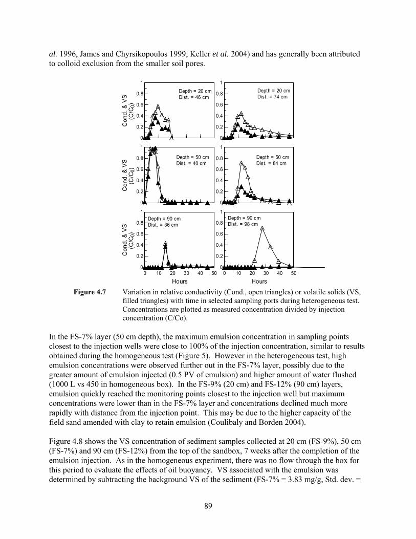
89

al. 1996, James and Chyrsikopoulos 1999, Keller et al. 2004) and has generally been attributed to colloid exclusion from the smaller soil pores.

0

0.2

0.4

0.6

0.8

1

0

0.2

0.4

0.6

0.8

1

Con

d. &

VS

(C

/C0)

Depth = 20 cmDist. = 74 cm


0

0.2

0.4

0.6

0.8

1

0

0.2

0.4

0.6

0.8

1

Con

d. &

VS

(C

/C0)



0 10 20 30 40 50

Hours

0

0.2

0.4

0.6

0.8

1

0 10 20 30 40 50

Hours

0

0.2

0.4

0.6

0.8

1

Con

d. &

VS

(C

/C0)



Figure 4.7 Variation in relative conductivity (Cond., open triangles) or volatile solids (VS,

filled triangles) with time in selected sampling ports during heterogeneous test. Concentrations are plotted as measured concentration divided by injection concentration (C/Co).

In the FS-7% layer (50 cm depth), the maximum emulsion concentration in sampling points closest to the injection wells were close to 100% of the injection concentration, similar to results obtained during the homogeneous test (Figure 5). However in the heterogeneous test, high emulsion concentrations were observed further out in the FS-7% layer, possibly due to the greater amount of emulsion injected (0.5 PV of emulsion) and higher amount of water flushed (1000 L vs 450 in homogeneous box). In the FS-9% (20 cm) and FS-12% (90 cm) layers, emulsion quickly reached the monitoring points closest to the injection well but maximum concentrations were lower than in the FS-7% layer and concentrations declined much more rapidly with distance from the injection point. This may be due to the higher capacity of the field sand amended with clay to retain emulsion (Coulibaly and Borden 2004). Figure 4.8 shows the VS concentration of sediment samples collected at 20 cm (FS-9%), 50 cm (FS-7%) and 90 cm (FS-12%) from the top of the sandbox, 7 weeks after the completion of the emulsion injection. As in the homogeneous experiment, there was no flow through the box for this period to evaluate the effects of oil buoyancy. VS associated with the emulsion was determined by subtracting the background VS of the sediment (FS-7% = 3.83 mg/g, Std. dev. =

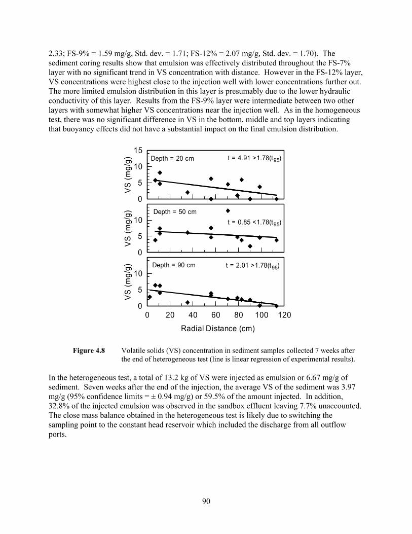
90

2.33; FS-9% = 1.59 mg/g, Std. dev. = 1.71; FS-12% = 2.07 mg/g, Std. dev. = 1.70). The sediment coring results show that emulsion was effectively distributed throughout the FS-7% layer with no significant trend in VS concentration with distance. However in the FS-12% layer, VS concentrations were highest close to the injection well with lower concentrations further out. The more limited emulsion distribution in this layer is presumably due to the lower hydraulic conductivity of this layer. Results from the FS-9% layer were intermediate between two other layers with somewhat higher VS concentrations near the injection well. As in the homogeneous test, there was no significant difference in VS in the bottom, middle and top layers indicating that buoyancy effects did not have a substantial impact on the final emulsion distribution.

0

5

10

VS

(mg/

g)

0 20 40 60 80 100 120

Radial Distance (cm)

0

5

10

VS (m

g/g) Depth = 90 cm

0

5

10

15

VS

(mg/

g) Depth = 20 cm

Depth = 50 cm

t = 2.01 >1.78(t 95)

t = 0.85 <1.78(t 95)

t = 4.91 >1.78(t 95)

Figure 4.8 Volatile solids (VS) concentration in sediment samples collected 7 weeks after the end of heterogeneous test (line is linear regression of experimental results).

In the heterogeneous test, a total of 13.2 kg of VS were injected as emulsion or 6.67 mg/g of sediment. Seven weeks after the end of the injection, the average VS of the sediment was 3.97 mg/g (95% confidence limits = ± 0.94 mg/g) or 59.5% of the amount injected. In addition, 32.8% of the injected emulsion was observed in the sandbox effluent leaving 7.7% unaccounted. The close mass balance obtained in the heterogeneous test is likely due to switching the sampling point to the constant head reservoir which included the discharge from all outflow ports.

91

4.4.3 Mathematical Modeling of Emulsion Transport and Immobilization Emulsion transport was simulated using MODFLOW (MacDonald and Harbaugh 1988) and RT3D (Clement 1997) as implemented in GMS 3.1 (Brigham Young University 1999) using the emulsion transport module previously developed in Section 4.3.3. This module assumes that emulsion transport and retention can be simulated using filtration theory with a Langmuirian blocking function to simulate saturation of the sediment surfaces with entrapped oil droplets. This approach does not consider changes in fluid density or viscosity associated with concentrated emulsions or permeability loss associated with droplet capture by sediment surfaces. The 3-D sandboxes were represented in plan view by a 20 x 20 grid where each cell was 5 cm x 5 cm. In the homogeneous experiments, the sandbox was simulated as a single vertical layer. In the heterogeneous experiments, the sandbox was represented by three separate layers. No flow and constant head boundary conditions were implemented where appropriate. Porosity was calculated from the sediment specific gravity and the dry weight of sediment added to each layer. For both the homogeneous and heterogeneous tests, the total transmissivity of sandbox was obtained by fitting water level monitoring results to the steady-state Thiem equation. For the heterogeneous test, the transmissivity of each layer was estimated based on the layer thickness and hydraulic conductivity measurements in standard laboratory permeameters (ASTM d 2434, 2000). Dispersivity was independently estimated by fitting MT3D (Zheng 1990) to match results from non-reactive tracer tests (calibration results not shown). Emulsion transport parameters, empty bed collision efficiency ( α’), and maximum oil retention per mass of sediment ( max

imC ), for FS-7%, FS-9% and FS-12% were obtained from previous measurements in the 1-D columns and used without any calibration. The model parameter values for FS-7% are the average of the four values shown in Table 4.2. Model parameter values for both the homogeneous and heterogeneous tests are presented in Table 4.3.

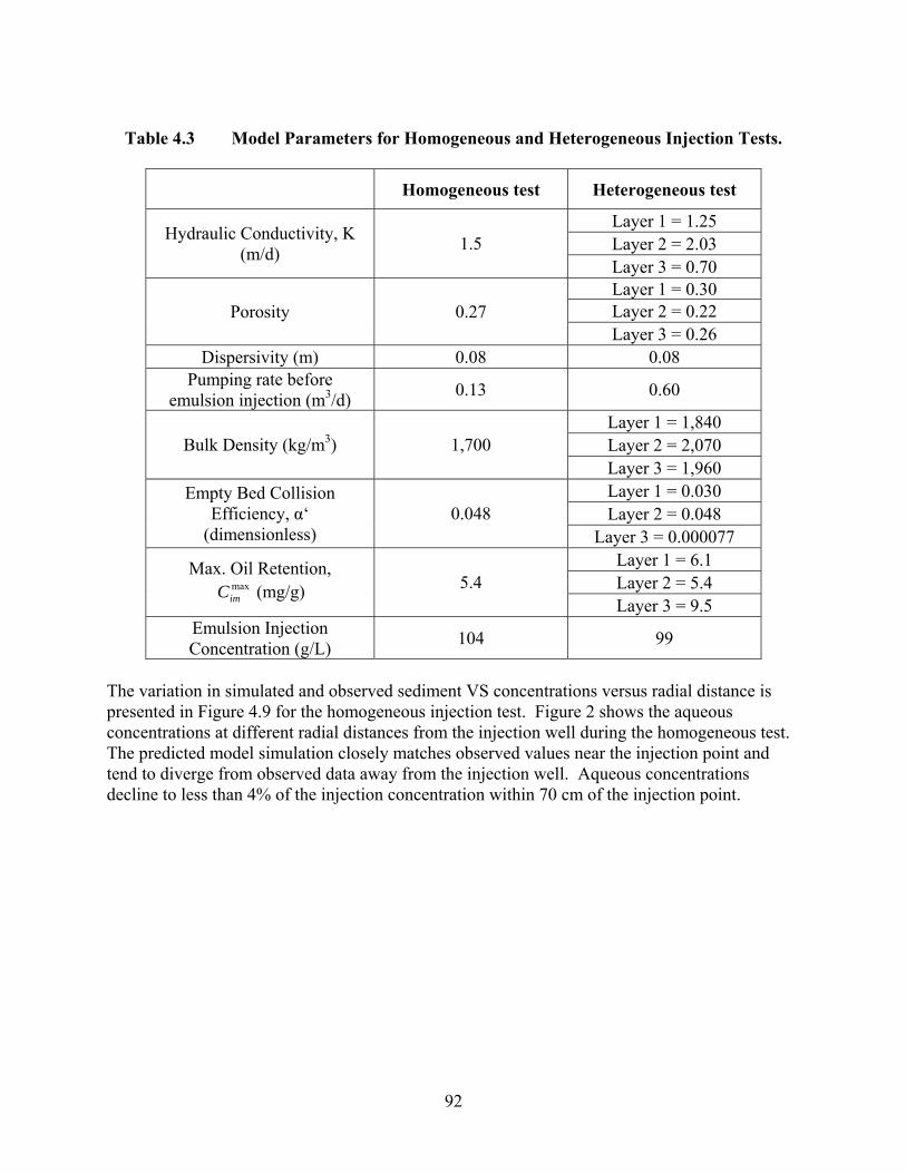
92

Table 4.3 Model Parameters for Homogeneous and Heterogeneous Injection Tests.

Homogeneous test Heterogeneous test

Layer 1 = 1.25 Layer 2 = 2.03 Hydraulic Conductivity, K

(m/d) 1.5 Layer 3 = 0.70 Layer 1 = 0.30 Layer 2 = 0.22 Porosity 0.27 Layer 3 = 0.26

Dispersivity (m) 0.08 0.08 Pumping rate before

emulsion injection (m3/d) 0.13 0.60

Layer 1 = 1,840 Layer 2 = 2,070 Bulk Density (kg/m3) 1,700 Layer 3 = 1,960 Layer 1 = 0.030 Layer 2 = 0.048

Empty Bed Collision Efficiency, α‘

(dimensionless) 0.048

Layer 3 = 0.000077 Layer 1 = 6.1 Layer 2 = 5.4

Max. Oil Retention, maximC (mg/g) 5.4

Layer 3 = 9.5 Emulsion Injection Concentration (g/L) 104 99

The variation in simulated and observed sediment VS concentrations versus radial distance is presented in Figure 4.9 for the homogeneous injection test. Figure 2 shows the aqueous concentrations at different radial distances from the injection well during the homogeneous test. The predicted model simulation closely matches observed values near the injection point and tend to diverge from observed data away from the injection well. Aqueous concentrations decline to less than 4% of the injection concentration within 70 cm of the injection point.

93

0 0.5 1 1.5Radial Distance (m)

0

3

6

9

VS

(mg/

g)

Figure 4.9 Variation in predicted (line) and observed (circles) sediment volatile solids (VS) concentration versus radial distance from the injection well for the homogeneous test. Observed concentrations are corrected for background VS.

Predicted and observed sediment VS concentrations at the end of the heterogeneous test are compared in Figure 4.10. Observed VS concentrations in the aqueous phase are compared to predicted model simulation in Figure 4.11. Throughout the middle FS-7% layer, the predicted values closely match the observed aqueous concentrations. In the upper FS-9% layer, the simulation closely matches observed concentrations close to the injection point. However there is greater discrepancy farther away from the injection point. In the lower FS-12% layer, the predicted simulation appears to match the aqueous measurements equally well.

0

5

10

15

VS

(mg/

g) FS-9%

0

5

10

VS

(mg/

g) FS-7%

0 0.5 1 1.5Radial Distance (m)

0

5

10

VS

(mg/

g) FS-12%

Figure 4.10 Variation in predicted (line) and observed (circles) sediment volatile solids (VS)

concentration versus radial distance from the injection well for the heterogeneous test. Observed concentrations are corrected for background VS.

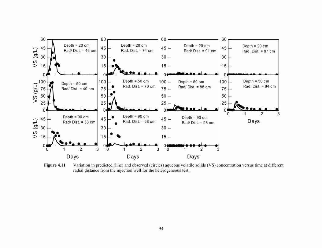
94

0

15

30

45

60VS

(g/L

)

0

15

30

45

60Depth = 20 cmRad. Dist. = 74 cm

Depth = 20 cmRad/ Dist. = 46 cm

0255075

100

0255075

100

VS

(g/L

) Depth = 50 cmRad. Dist. = 70 cm

0 1 2 3

Days

0

15

30

45


0 1 2 3

Days

0

15

30

45

VS

(g/L

) Depth = 90 cmRad. Dist. = 68 cm


0

15

30

45

60

0

15

30

45

60Depth = 20 cmRad. Dist. = 97 cm


0 1 2 3

Days

0255075

100

0255075

100 Depth = 50 cmRad. Dist. = 84 cm


0 1 2 3

Days

0

15

30

45 Depth = 90 cmRad/ Dist. = 98 cm

Figure 4.11 Variation in predicted (line) and observed (circles) aqueous volatile solids (VS) concentration versus time at different

radial distance from the injection well for the heterogeneous test.

95

Overall, the emulsion transport model provided a good prediction of the aqueous VS concentration versus time in multiple monitoring points and the final VS distribution in the sediment using independently measured parameter values. The only location where the model prediction is somewhat less than desired is for the FS+12% layer in the heterogeneous test. In this layer, the model predicts somewhat higher sediment VS concentrations than observed. The difference between simulated and observed VS concentrations could be due to higher uncertainties in the parameter estimates for this layer. In the 1-D columns, the higher clay content in FS-12% required higher injection pressures which could have resulted in some flow bypassing and less reliable parameter estimates for FS-12%. The empty bed collision efficiency (α’) value for FS-7% is an average of four column experiments where observed values of α’ varied from 0.02 to 0.07 indicating significant variability among replicate columns. These variations are not unreasonable given that prior investigators (Jewett et al. 1995) have reported 1 or 2 orders of magnitude variation in α’ in replicate bacterial transport experiments. The α’ values in the 1-D columns for the FS-9% and FS-12% were each generated from a single column experiment. Given the variability observed for FS-7%, the parameter estimates for FS-9% and FS-12% could be an order of magnitude higher or lower than single observed value. As discussed above, the independent estimates of α’ generally resulted in a good match with the aqueous emulsion measurements. 4.5 MODEL SENSITIVITY ANALYSIS A series of model simulations were performed to better understand the different factors controlling emulsified oil transport in the subsurface. In these simulations, we employed an idealized geometry consisting of a single injection well located in a 1 m thick confined aquifer. For the base condition, a 12% oil in water emulsion (20% dilution of EOS® concentrate) was injected for 0.1 days at a flow rate of 4000 L/d followed by chase water for 9.9 days. All other model parameters were identical to the lower aquifer layer at the field site (Table 4.1). Figure 4.12 shows simulated aqueous and sorbed oil concentrations as a function of distance from the injection well. Immediately following emulsion injection (0.1 day), aqueous concentrations are high and little oil is adsorbed to the sediment. As the chase water pushes the emulsified oil droplets farther out into the aquifer, aqueous concentrations decline due to dilution and attachment of oil droplets to the sediment surfaces. Within one day, peak aqueous concentrations have declined by 95% and the emulsion peak has been pushed away from the injection well by chase water. Continued injection of chase water from 1 to 10 days moves a small portion of the oil farther away from the injection well where it is eventually captured by the aquifer sediment. After 10 days, essentially all of the injected oil has been captured by the aquifer sediment.

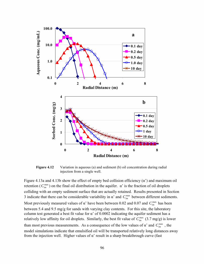
96

0.1

1.0

10.0

100.0

0 2 4 6 8Radial Distance (m)

Aqu

eous

Con

c. (m

g/m

L)

0.1 day0.2 day0.5 day1.0 day10 day

a

0

1

2

3

4


Sorb

ed C

onc.

(mg/

g)

0.1 day0.2 day0.5 day1 day10 day

b

Figure 4.12 Variation in aqueous (a) and sediment (b) oil concentration during radial injection from a single well.

Figure 4.13a and 4.13b show the effect of empty bed collision efficiency (α’) and maximum oil retention ( max

imC ) on the final oil distribution in the aquifer. α’ is the fraction of oil droplets colliding with an empty sediment surface that are actually retained. Results presented in Section 3 indicate that there can be considerable variability in α’ and max

imC between different sediments. Most previously measured values of α’ have been between 0.02 and 0.07 and max

imC has been between 5.4 and 9.5 mg/g for sands with varying clay contents. For this site, the laboratory column test generated a best fit value for α’ of 0.0002 indicating the aquifer sediment has a relatively low affinity for oil droplets. Similarly, the best fit value of max

imC (3.7 mg/g) is lower than most previous measurements. As a consequence of the low values of α’ and max

imC , the model simulations indicate that emulsified oil will be transported relatively long distances away from the injection well. Higher values of α’ result in a sharp breakthrough curve (fast

97

attachment kinetics) with more of the oil is retained close to the injection well. Low values of maximC allow a larger portion of the oil to migrate more than 8 m from the injection point.

0

1

2

3

4


Sorb

ed C

onc.

(mg/

g)

α' = 0.00002α' = 0.0002α' = 0.002

a

0

1

2

3

4

5


Sorb

ed C

onc.

(mg/

g)

Max. Oil Retent. = 1.0 mg/gMax. Oil Retent. = 3.7 mg/gMax. Oil Retent. = 10.0 g/g

b

Figure 4.13 Effect of: (a) empty bed collision efficiency (α’); and (b) maximum oil retention ( max

imC ) on the final oil distribution in sediment following radial injection for 10 days.

Figure 4.14 shows the effect of injection conditions on the final oil distribution in the aquifer. Increasing the amount of oil injected from 24 Kg to 240 Kg per m of aquifer thickness substantially increases the amount of oil in the 2 to 4 m region and moves some additional oil over 8 m from the injection point (Figure 8a). In contrast, increasing the injection well flow rate from 2000 to 8000 L/d per m of aquifer had a minor impact on the final oil distribution (Figure 8b). Figure 8c shows that if the total amount of oil is held constant, diluting the oil with more water (changing the emulsion concentration from 6% to 30%) will have no effect on the final oil distribution.

98

0

1

2

3

4

5


Sorb

ed C

onc.

(mg/

g)

24 Kg oil48 Kg oil240 Kg oil

a

0

1

2

3

4


Sorb

ed C

onc.

(mg/

g)

2000 L/d4000 L/d8000 L/d

b

0

1

2

3

4


Sorb

ed C

onc.

(mg/

g)

800 L of 6% oil400 L of 12% oil160 L of 30% oil

c

Figure 4.14 Effect of: (a) amount of oil injected; (b) injection flowrate; and (c) pulsed

injection on final oil distribution in sediment following radial injection for 10 days.

99

4.6 SUMMARY The laboratory column experiments demonstrated that soybean oil-in-water emulsions prepared with small, uniformly sized droplets and a negative surface charge can be distributed in sands with varying clay content at least 80 cm away from the injection point. The approach of injecting a concentrated pulse of emulsion followed by chase water to distribute and immobilize the oil droplets provided a reasonably uniform final oil distribution when sufficient oil was injected. Residual oil concentrations varied from 1 to 9 mg/g VS and should be effective for stimulating in situ anaerobic bioremediation processes. The maximum residual oil concentrations resulting from a short pulse injection were generally consistent with prior work by Coulibaly and Borden (2004) where columns were flushed with at least three PVs of concentrated emulsion. At present, we have a very poor understanding of the physical and chemical processes controlling droplet capture and retention by the sediment surfaces. The emulsions used in this work had a negative zeta potential and can be expected to attach poorly to negatively charged sands. However, natural sediments including iron oxide coated sands and clay minerals have a mixture of positively and negatively charged sites which could allow more effective capture of small, negatively charged oil droplets. We anticipate that most of the surfactants used to prepare the emulsion will be associated with the oil droplet surface. However, a small portion of the surfactant will be dissolved and could sorb to sediment surfaces, potentially altering their surface properties. A mathematical model based on traditional colloid transport approaches is presented for simulating the transport and retention of emulsions in laboratory columns. The model provides an adequate description of effluent breakthrough curves and the final oil distribution in laboratory columns packed with field sand containing 7%, 9% and 12% silt and clay size material. Empty bed collision efficiencies measured in replicate columns and at varying velocities were reasonably reproducible and generally consistent with prior work on bacterial transport in aquifer material. Kaolinite addition to field sand increased the maximum oil retention. However, empty bed collision efficiencies in columns packed with field sand amended with kaolinite were lower than in columns packed with field sand only suggesting that kaolinite is a less efficient collector of oil droplets than the natural clayey sand. The model employed in this work is based on several important assumptions: (1) transport of dissolved VS is not significant, and (2) oil droplets are irreversibly captured by the sediment surfaces. During the early portion of the flushing experiments, most VS are present in oil droplets and transport of dissolved components is relatively unimportant. However during the later stages of flushing when oil droplet transport declines, dissolved oil and surfactants will make up a much larger fraction of the VS. Consequently, it is not appropriate to use the emulsion transport model to simulate the slow release of dissolved components that occurs towards the end of the injection experiments. Attempts to simulate release of dissolved organic material will be further complicated by growth of bacteria which ferment soybean oil to more soluble fatty acids, accelerating organic carbon release (Chapter 3). Biotransformation processes

100

will also alter the aquifer Eh and pH, reducing iron and manganese oxides, potentially influencing oil droplet capture and/or release by sediment surfaces. Large-scale 3-D sandbox experiments were conducted for both homogeneous and heterogeneous conditions to evaluate the transport and distribution of emulsified edible oils under controlled laboratory conditions. Results from this work showed that injection of a fine oil-in-water emulsion (~ 0.1 PV for homogeneous, ~ 0.5 PV for heterogeneous) followed by chase water (~ 1.5 PV for homogeneous, ~ 5.5 PV for heterogeneous) resulted in excellent oil distribution throughout fine clayey sand with no permanent reduction in hydraulic conductivity and no upward movement of the oil due to buoyancy effects. Data from both of these tests were used to evaluate a numerical model of emulsion transport. The emulsion transport model was calibrated using parameter values independently measured in the 1-D column experiments. Model predictions for both the homogeneous and heterogeneous injection tests generally matched observed values. These results indicate that the transport and distribution of emulsified oil can be simulated using a colloidal transport model which incorporates a Langmuirian blocking function to simulate the effects of sediment surface saturation with attached emulsion droplets. This model was implemented as a user-defined module in RT3D. The validated model was was then used to evaluate the effect of aquifer parameters and injection conditions on the resulting oil distribution. Model simulations indicate that the final oil distribution in the aquifer will be sensitive to the empty bed collision efficiency and maximum oil retention. These parameters vary considerably from one site to the next. Consequently, accurate prediction of the oil distribution at a field site will like require site specific laboratory column tests. Model sensitivity analyses indicate that the spread of emulsified oil away from the injection well can be enhanced by injecting more oil. However, increasing the injection flow rate or diluting the oil with more water will have little effect on final oil distribution in the aquifer. Additional work is needed to understand the various processes controlling oil droplet capture by different sediments and subsequent release of dissolved organic carbon to support in situ biotransformation processes. As our understanding improves, it may be possible to control oil droplet mobility by matching the surfactant selected to the specific physical and chemical properties of the aquifer. This information could then be incorporated into mathematical models as an aid in the design of emulsion injection systems.

101

4.7 REFERENCES AFCEE. 2004. Principles and Practices of Enhanced Anaerobic Bioremediation of Chlorinated

Solvents, Air Force Center for Environmental Excellence, Brooks Air Force Base, Texas. ASTM (American Society for Testing and Materials). 2000. Designation: D 2434-68, Standard

Test Method for Permeability of Granular Soils (Constant Head), West Conshohocken, PA.

Becker, M.W., Collins S.A., Metge D.W., Harvey R.W., and Shapiro A.M. 2004. “Effect of cell

physicochemical characteristics and motility on bacterial transport in groundwater.” J. Contam. Hydro., 69 (3-4), 195-213.

Bengtsson, G., and Ekere, L. 2001. “Predicting sorption of groundwater bacteria from size

distribution, surface area, and magnetic susceptibility of soil particles.” Wat. Resour. Res., 37(6), 1795-1812.

Bengtsson, G., and Lindqvist, R. 1995. “Transport of soil bacteria controlled by density

dependent sorption kinetics.” Wat. Resour. Res., 31(5), 1247-1256. Bolster, C. H., Hornberger, G. M., Mills, A. L., and Wilson, J. L. 1998. “A method for

calculating deposition coefficients using the fraction of bacteria recovered from laboratory columns.” Environ. Sci. Technol., 32(9), 1329-1332.

Bolster, C. H., Mills, A. L., Hornberger, G. M., and Herman, J. S. 2001. “Effect of surface

coatings, grain size, and ionic strength on the maximum attainable coverage of bacteria on sand surfaces.” J. Cont. Hydro., 50(1-4), 287-305.

Brigham Young University, Environmental Modeling Laboratory, 1999. The Department of

Defense Groundwater Modeling System, GMS v3.1. Camesano, T. A., and Logan, B. E. 1998. “Influence of fluid velocity on cell concentration and

the transport of motile and nonmotile bacteria.” Envir. Sci. Technol., 32(11), 1699-1709. Camesano, T. A., Unice, K. M., and Logan, B. E. 1999. “Blocking and ripening of colloids in

porous media and their implications for bacterial transport.” Colloids and surfaces A: Physicochem. Engr. Asp., 160(3), 291-308.

Casey, C. C., Reed, J., Britto, R., Stedman, J., Henry, B., and Wiedemeier, T. 2002. “Field-Scale

Evaluation of Soybean Oil and Dissolved Substrates for In-Situ Bioremediation.” Third International Conference on Remediation of Chlorinated and Recalcitrant Compounds, Battelle Press, Monterey, CA.

102

Chen, J. Y., Ko, C. H., Bhattacharjee, S., and Elimelech, M. 2001. “Role of spatial distribution of porous medium surface charge heterogeneity in colloid transport.” Colloids and surfaces A: Physicochem. Engr. Asp., 191(1-2), 3-15.

Clement, T. P. 1997. RT3D – A modular computer code for simulating reactive multi-species

transport in 3-Dimensional groundwater aquifers, Battelle Pacific Northwest National Laboratory Research Report, PNNL-SA-28967.

Coulibaly, K. M., and Borden, R. C. 2004 “Impact of edible oil injection on the permeability of

aquifer sands.” J. Cont. Hydrol., 71(1-4), 219– 237. Coulibaly, K. M., Long, C. M., and Borden, R. C., 2006. “Subsurface transport of edible oil

emulsions: 1-D column results and model development.” J. Engr. Hydrology.. 11(3):230-237, 2006.

Elimelech, M. and Omelia, C. R. 1990. “Kinetics of deposition of colloidal particles in porous

media.” Envir. Sci. Technol. 24(10), 1528-1536. Enfield, C. G., Bengtsson, G., and Lindqvist, R. 1989. “Influence of macromolecules on

chemical transport.” Environ. Sci. Technol. 23(10), 1278-1286. Grindrod, P. 1993. “The impact of colloids on the migration and dispersal of radionuclides

within fractured rock.” J. Contam. Hydrol. 13(1-4), 167-182. Grindrod, P., Edwards, M. S., Higgo, J. J. W., and Williams, G. M. 1996. “Analysis of colloid

and tracer breakthrough curves.” J. Contam. Hydrol. 21(1-4), 243-253. Higgo, J. J. W., Williams, G. M., Harrison, I., Warwick, P., Gardiner, M. P., and Longworth, G.

1993. “Colloid transport in a glacial sand aquifer. Laboratory and field studies.” Colloids and Surfaces A. 73, 179-200.

Huber, N., Baumann, T., and Niessner, R. 2000. “Assessment of colloid filtration in natural

porous media by filtration theory.” Envir. Sci. Technol., 34(17), 3774-3779. Hunter, W. J. 2001. “Use of vegetable oil in a pilot-scale denitrifying barrier.” J. Cont. Hydro.,

53(1-2), 119-131. Hunter, W. J. 2002. “Bioremediation of chlorate or perchlorate contaminated water using

permeable barriers containing vegetable oil.” Current Microbiol., 45(4), 287-292. Interstate Technology and Regulatory Council (ITRC) In Situ Bioremediation Team 2002.

Technical/Regulatory Guidelines: A Systematic Approach to In Situ Bioremediation in Groundwater including Decision Trees on In Situ Bioremediation for Nitrates, Carbon Tetrachloride, and Perchlorate.

103

James, S.C., and Chrysikopoulos, C. V. 1999. “Transport of polydisperse colloid suspensions in a single fracture.” Wat. Resour. Res., 35(3), 707-718.

Jewett, D. G., Hilbert, T. A., Logan, B. E., Arnold, R. G., and Bales, R. C. 1995. “Bacterial

transport in laboratory columns and filters: influence of ionic strength and pH on collision efficiency.” Wat. Res., 29(7), 1673-1680.

Johnson, P. R., and Elimelech, M. 1995. “Dynamics of colloid deposition in porous media:

blocking based on random sequential adsorption.” Langmuir, 11(3), 801-812. Johnson W. P., Blue, K. A., Logan, B. E., and Arnold, R. G. 1995. “Modeling bacterial

detachment during transport through porous-media as a residence-time-dependent approach.” Water Resourc. Res. (11) 2649-2658.

Johnson, P. R., Sun, N., and Elimelech, M. 1996. “Colloid transport in geochemically

heterogeneous porous media: Modeling and measurements.” Environ. Sci. Technol. 30(11), 3284-3293.

Keller, A.A., Sirivithayapakorn, S., and Chrysikopoulos, C. V. 2004. “Early breakthrough of

colloids and bacteriophage MS2 in a water saturated sand column.” Wat. Resour. Res., 40(8), Art. No. W08304.

Ko, C. H., and Elimelech, M. 2000. “The “shadow effect” in colloid transport and deposition

dynamics in granular porous media: mechanisms and measurements” Environ. Sci. Technol. 34(17), 3681-3689.

Ko, C. H., Bhattacharjee, S., and Elimelech, M. 2000. “Coupled influence of colloidal and

hydrodynamics interactions on the RSA dynamic blocking function for particle deposition onto packed spherical collectors” J. Colloid Interface Sci. 229(2), 554-567.

Lee, D. M., Lieberman, T. M., Borden, R. C., Beckwith, W., Crotwell, T., and Haas, P. E. 2001.

“Effective distribution of edible oils – results from five field applications, In G. B. Wickramanayake, A. R. Gavaskar, B. C. Alleman and V. S. Magar (Eds.), Proc. In Situ and On-Site Bioremediation: The Sixth Internal. Sym., San Diego, CA.

Lindqvist, R., Cho, J. S., and Enfield, C. G. 1994. “A kinetic model for cell density dependent

bacterial transport in porous media.” Wat. Resourc. Res., 30(12), 3291-3299. Logan, B.E. 1999. Environmental Transport Processes, John Wiley & Sons, New York. Martin, J. M., Logan, B. E., Johnson, W. P., Jewett, D. G., and Arnold, R.G. 1996. “Scaling

bacterial filtration rates in different sized porous media.” J. Env. Eng., 122(5), 407-415. McDonald, J. M. and Harbaugh, A. W. 1988. “A modular three-dimensional finite-difference

groundwater flow model.” Techniques of water resources investigations of the U.S. Geological Survey Book 6.

104

Meinders, J. M., Noordmans, J., and Busscher, H. J. 1992. “Simultaneous monitoring of

adsorption and desorption of colloidal particles during deposition in a parallel plate flow chamber.” J. Colloid Interface Sci. 152(1), 265-280.

Meinders, J.M., vanderMei, H.C., Busscher, H. J. 1995. “Deposition efficiency and reversibility

of bacterial adhesion under flow.” J. Colloid Interface Sci. 176(2), 329-341. Morse, J. J., Alleman, B. C., Gossett, J. M., Zinder, S. H., Fennell, D. E., Sewell, G. W., and

Vogel, C. M. 1998. Draft Technical Protocol: A Treatability Test for Evaluating the Potential Applicability of the Reductive Anaerobic Biological In Situ Treatment Technology (RABITT) to Remediate Chloroethenes, Environmental Technology Certification Program, Washington, DC.

Rajagopalan, R., and Tien, C. 1976. “Trajectory analysis of deep-bed filtration with the sphere-

in-cell porous media model.” A.I.C.H.E.J. 22(3), 523-533. Rijnaarts, H. H. M., Norde, W., Bouwer, E. J., Lyklema, J., and Zehnder, A. J. B. 1996a.

“Bacterial deposition in porous media: Effects of cell-coating, substratum hydrophobicity, and electrolyte concentration.” Envir. Sci. Technol., 30, 2877-2883.

Rijnaarts, H. H. M., Norde, W., Bouwer, E. J., Lyklema, J., and Zehnder, A. J. B. 1996b.

“Bacterial deposition in porous media related to the clean bed collision efficiency and to substratum blocking by attached cells.” Environ. Sci. Technol., 30(10), 2869-2876.

Ryan, J. N., and Elimelech, M. 1996. “Colloid mobilization and transport in groundwater.”

Colloids and Surfaces: A-Physicochem. Engr. Asp. 107, 1-56. Sabbodish, M.S. Jr. 2002. A Physicochemical Investigation of the Soil Clogging Phenomena

During Surfactant Enhanced Remediation. Doctoral Dissertation, Dept. Civil Engr., North Carolina State Univ.

Sim, Y., and Chrysikopoulos, C. V. 1995. “Analytical models for one-dimensional virus

transport in saturated porous media.” Water Resour. Res., 31(5), 1429-1437. Sim, Y., and Chrysikopoulos, C. V. 1998. “Three-dimensional analytical models for virus

transport in saturated porous media.” Transport in Porous Media, 30(1), 87-112. Soo, H., and Radke, C. J. 1984. “The flow mechanism of dilute stable emulsions in porous

media.” Ind. Eng. Chem. Fundam., 23(3), 342-347. Soo, H., and Radke, C.J. 1986a. “A filtration model for the flow of dilute stable emulsions in

porous media – I. Theory.” Chem. Engr. Sci. 41(2), 263-272.

105

Soo, H., and Radke, C. J. 1986b. “A filtration model for the flow of dilute stable emulsions in porous media – II. Parameter evaluation and estimation.” Chem. Engr. Sci., 41(2), 273-281.

Westall, J. C., and Gschwend, P. M. 1993. “Mobilizing and depositing colloids.” Manipulation

of groundwater colloids for Environmental Restoration, Lewis Publishers, Ann Harbor. Zenker, M. J., Borden, R. C., Barlaz, M. A., Lieberman, M. T., and Lee, M. D. 2000. “Insoluble

substrates for reductive dehalogenation in permeable reactive barriers.” Bioremediation and Phytoremediation, Eds: G. B. Wickramanayake, A. R. Gavaskar, B. C. Alleman and V. S. Magar, p. 47-53, Battelle Press, Columbus, OH.

Zheng, C. 1990. MT3D - A Modular Three-Dimensional Transport Model for Simulation of

Advection, Dispersion and Chemical Reactions of Contaminants in Groundwater System. U.S. Environmental Protection Agency, Ada, OK.

106

CHAPTER 5: EFFECTIVE DISTRIBUTION OF EMULSIFIED EDIBLE

OIL FOR ENHANCED ANAEROBIC BIOREMEDIATION 5.1 INTRODUCTION In-situ anaerobic bioremediation have been proposed for remediation of a variety of groundwater contaminants including chlorinated aliphatic hydrocarbons (CAHs), perchlorate (ClO4), chromate, nitrate, high explosives and radionuclides (Lee et al., 1998; Ellis et al., 2000; Hunter, 2001, 2002; Major et al., 2002; AFCEE and NFESC, 2004; May et al., 2004; Nevin et al., 2003). All of these processes require that the contaminant be brought in contact with a biodegradable organic substrate. This substrate may be used directly or may be fermented to hydrogen (H2) and low-molecular weight fatty acids providing carbon and energy sources for the target anaerobic biotransformation processes. 5.1.1 Perchlorate Extent and Degradation Groundwater and surface water contamination with perchlorate has become a major environmental issue due to the use, release and/or disposal of solid rocket fuel, munitions and pyrotechnics containing ammonium perchlorate. These releases have resulted in extensive contamination of surface and groundwater supplies. In the western US, over 15 million people consume water with some level of perchlorate. This is a significant concern because high levels of perchlorate interfere with iodide uptake by the thyroid. As of 2006, the U.S. Environmental Protection Agency (USEPA) has not established a maximum contaminant level (MCL) for perchlorate in drinking water. However, USEPA published a human reference dose (RfD) for perchlorate at 0.0007 milligrams/kilogram/day (mg/kg/D) which results in a drinking water equivalent level (DWEL) of 24.5 parts per billion (ppb), assuming all of a contaminant comes from drinking water (EPA 542-R05-015; ITRC Perchlorate Team, 2005). In addition, several states have identified advisory levels for perchlorate that range from 1 µg/L to 52 µg/L (ITRC Perchlorate Team, 2005). Perchlorate is a highly mobile, soluble salt that sorbs poorly to most aquifer materials and can persist for decades under aerobic conditions. However under anaerobic conditions, perchlorate can be used as an electron acceptor by a variety of different bacteria. In this process, perchlorate is degraded through the following sequence. ClO4

- (perchlorate) ClO3- (chlorate) ClO2

- (chlorite) Cl- (chloride) + O2 (oxygen) A variety of facultatively anaerobic, perchlorate-reducing bacteria have been isolated, many of which are members of the newly identified genera Dechloromonas, Dechlorospirillum, and Azospira (formerly Dechlorosoma) (Achenbach et al., 2001; Xu et al., 2003). Perchlorate-reducing organisms are widespread in the environment (Coates et al., 1999; Logan, 2001) and can use a variety of different organic substrates as electron donors including fatty acids (e.g., acetate, citrate, lactate), mixed and pure sugars (e.g., molasses, glucose), protein-rich substrates (whey, casamino acids), alcohols (e.g., ethanol), vegetable oils, and hydrogen gas (Logan, 1998;

107

Hunter, 2002; Waller et al., 2004; Zhang et al., 2002; Hatzinger, 2005). Perchlorate reduction occurs under facultative anaerobic conditions and is inhibited by dissolved oxygen concentrations in excess of 2 mg/L (Rikken et al., 1996; Chaudhuri et al., 2002). However, when biodegradable organic substrates are present, the available dissolved oxygen will be consumed and perchlorate is rapidly biodegraded. 5.1.2 1,1,1-Trichloroethane Degradation 1,1,1-Trichloroethane (TCA) is resistant to aerobic biodegradation, but can be reductively dechlorinated to 1,1-dichloroethane (DCA) and then to chloroethane (CA) (Vogel and McCarty, 1987). Sun et al. (2002) demonstrated that reductive dechlorination of TCA was coupled to growth by Dehalobacter sp. str. TCA1. However, organisms that can dechlorinate CA to ethane have not yet been identified and CA does accumulate in some systems. In addition to reductive dechlorination, TCA and CA can also be degraded through abiotic hydrolysis reactions (McCarty and Semprini, 1994). Abiotic TCA transformation occurs via two different pathways leading to the production of roughly 20% 1,1-DCE and 80% acetic acid (HAc) with reported TCA half-lives vary from 0.95 yr at 20 ºC to 12 yr at 10 ºC (McCarty, 1996). CA reportedly hydrolyzes to ethanol (Vogel and McCarty, 1987; Vogel et al., 1987) with a half-life of 0.12 years. The relatively short half-life for CA hydrolysis may explain the disappearance of CA in systems where TCA is reductively dechlorinated to DCA and CA. 5.1.3 Anaerobic Biodegradation using Emulsified Oils Recent research has shown that edible oils including soybean oil and hydrogenated soybean oil can be used to enhance the anaerobic biodegradation of a variety of contaminants including nitrate (Lindow, 2004; Hunter, 2001), perchlorate (Hunter, 2002), chlorinated solvents (Zenker et al., 2000; AFCEE and NFESC, 2004; Long and Borden, 2006; Borden and Rodriguez, 2006), TNT, RDX and HMX (Fuller et al., 2004), acid mine drainage (Lindow and Borden, 2005) and chromium immobilization (Lindow, 2004). Once injected into the subsurface, the oil is believed to be first hydrolyzed releasing glycerol (an alcohol) and long-chain fatty acids (LCFAs) (Long and Borden, 2006; Hanaki et al., 1981). Glycerol is easy to biodegraded and very soluble, so this material will be quickly degraded or flushed out of the system. The LCFAs are much less soluble in water (Ralston and Hoerr, 1942) and are thought to initially sorb to sediment surfaces, followed by slow beta oxidation, releasing acetate and H2 (Sawyer et al., 1994). The acetate and H2 may then be used for contaminant reduction. Once injected, the emulsified oil can last extended time periods, supporting complete reductive dechlorination of PCE and TCE to ethene (Lee et al., 2003, Long and Borden, 2006). While edible oils appear to have many advantages for in situ anaerobic bioremediation, questions remain about the most effective approach for distribution of these materials in the subsurface. Boulicault et al. (2000) describe the injection of NAPL soybean oil as a carbon source to stimulate in situ reductive dechlorination. However, other workers (Zenker et al., 2000; Lee et al., 2001) have reported difficulties in effectively distributing NAPL soybean oil without excessive permeability loss. This is supported by the laboratory studies of Coulibaly and Borden (2004) who found that injection of pure liquid soybean oil into sands resulted in high oil residual

108

saturations with large permeability losses. In contrast, an oil-in-water emulsion with small, uniform droplets could easily be prepared using soybean oil and non-ionic surfactants approved for direct incorporation into food. Injection of this emulsion into sands with up to 10% clay resulted in much lower oil retention with low to moderate permeability loss (Coulibaly and Borden, 2004). In subsequent work, Coulibaly et al. (2006) and Jung et al. (2006) demonstrated that emulsion transport and retention in 1-D columns and 3-D sandboxes could be simulated using a conventional colloid transport approach modified to include a Langmuirian blocking function to simulate the effects of surface saturation by attached oil droplets. 5.1.4 Field Pilot Test of Emulsified Oil Biobarrier In this chapter, we describe the results of a field pilot test of the emulsified oil biobarrier at a perchlorate and chlorinated solvent impacted site. The emulsion transport model described in Chapter 4 is used to simulate the residual oil distribution following emulsion injection. Following installation of the PRBB, the measured residual oil distribution in the aquifer is compared with simulation results to evaluate the predictive accuracy of the model. The effects of PRBB installation on groundwater flow, biogeochemical conditions and contaminant concentrations are described. Major issues addressed in this work include: (1) evaluating the extent of contaminant degradation and electron acceptor consumption in a strongly oxidizing aquifer; (2) evaluating the potential for flow bypassing around the biobarrier due to permeability loss associated with oil injection and resulting biological activity; (3) estimating rates of substrate consumption and barrier longevity; and (4) comparison of observed contaminant degradation with numerical simulation results. 5.2 SITE CHARACTERISTICS AND BIOBARRIER INSTALLATION The pilot test site was conducted in a shallow unconfined aquifer impacted by ammonium perchlorate and waste solvent released from a former surface impoundment. The facility has been used for industrial purposes, such as fireworks manufacturing, munitions production, pesticide production, and research and manufacturing of solid propellant rockets. The primary contaminants of concern at the pilot-test site are perchlorate (ClO4) and 1,1,1-trichloroethane (TCA) with lesser amounts of trichloroethene (TCE) and related chlorinated volatile organic compounds (CVOCs). These materials were released from a small 10 m x 10 m x 2 m deep surface impoundment that was closed in 1988. A pump and treat system was installed shortly after closure of the surface impoundment to remediate the shallow aquifer. This system consists of a 30 m long groundwater extraction trench located 60 m downgradient of the former impoundment, a shallow-tray air stripper to remove chlorinated VOCs, and a 30 m long groundwater infiltration trench to recirculate treated water located 100 m upgradient of former impoundment. This system has removed significant amounts of TCA and TCE with a gradual decline in CVOC concentrations in groundwater. However, ClO4 is not efficiently removed in the air stripper and ClO4 concentrations in groundwater remain elevated.

109

The water table aquifer at the site is composed of silty sand and gravel to approximately 5 m below ground surface (BGS) and is underlain by silty clay. The primary contaminated zone appears to be this sand and gravel layer. Groundwater flow in the pilot test area is generally to the west towards the interceptor trench. The water table varies between approximately 0.3 and 3 m BGS. The groundwater flow velocity in the immediate vicinity of the proposed pilot test area was not well known prior to initiating the field test activities. Slug tests conducted on MW-3 in 1990 indicated a hydraulic conductivity of 0.1 m/d. However, based on the extraction and injection rates for the pump-and-treat system, the groundwater velocity appeared to be substantially higher. Subsequent specific capacity tests in injection and monitor wells throughout the site indicated an average hydraulic conductivity of 7 m/day. Approximately 20 months after emulsion injection, the groundwater extraction system was shut down due to the dramatic reductions in contaminant concentrations passing through the biobarrier, and somewhat increased operation and maintenance costs associated with increased iron and manganese concentrations. When the extraction system was shut down, the hydraulic gradient in the vicinity of the barrier declined from ~ 0.9% (std. dev. = 0.3%) to 0.2% with a decline in the groundwater flow velocity from ~ 122 m/yr (std. dev. = 47 m/yr) to 28-50 m/yr during the last two sampling events (assuming ave. K = 7 m/d, n=0.18). Prior to emulsion injection, the aquifer was aerobic, with positive oxygen-reduction potential (ORP), and significant levels of nitrate, perchlorate and CAHs, and low or non-detectable levels of reduced species (TOC, Mn, Fe, CH4). Concentration of DCA, CA, cis-DCE, VC were much lower than the parent compounds (TCA and TCE) indicating that reductive dechlorination was not a significant attenuation mechanism at this site. However, appreciable levels of 1,1-DCE were present in the aquifer, indicating some abiotic hydrolysis of TCA (McCarty, 1996). A 15 m wide pilot-scale biobarrier was installed approximately 13 m upgradient of the groundwater extraction trench (Figure 5.1) and monitored to evaluate removal of ClO4 in the biobarrier, prior to groundwater entering the extraction trench. The pilot-scale barrier is shorter than the groundwater extraction trench so groundwater flow is approximately one-dimensional and perpendicular to the biobarrier.

110

Figure 5.1 Pilot test layout showing general groundwater flow direction, emulsion injection

points, soil sampling locations, extraction trench, injection and monitor wells.

111

The biobarrier was constructed by first installing ten shallow wells spaced 1.5 m on-center in a line parallel to the groundwater extraction trench. Each well was constructed of 2.5 cm diameter PVC casing with #20 slotted PVC screen extending from 1.8 to 4.9 m BGS. All wells were installed by direct push and completed with a bentonite seal and flush mount cover. Prior to emulsion injection, a non-reactive tracer test was conducted by injecting 3,300 L of NaBr solution (517 mg/L as Br) through a monitor well located 2 m upgradient of the biobarrier and monitoring Br breakthrough in the injection and monitor wells. In October 2003, emulsified soybean oil was injected to form the biobarrier. 42 L (11 gal.) of the pre-blended concentrated emulsion (Emulsified Oil Substrate or EOS®) was diluted with 166 L (44 gal.) of water and injected into each well followed by 625 L (165 gal.) of chase water to distribute and immobilize the emulsion. The total amount of emulsion injected was selected to provide sufficient substrate to degrade the target contaminants over a two-year monitoring period, with little or no-excess. By injecting a relatively small amount of emulsified oil (416 L or 2 just drums), we hoped to provide more precise estimates of substrate life. In a full-scale remediation project, sufficient substrate would normally be injected to last 5 to 10 years. The EOS® concentrate consists of approximately 60% soybean oil, 24% water, 2% yeast extract, 10% emulsifier, 4% lactic acid / sodium lactate (www.EOSRemediation.com). The emulsion is prepared using high energy mixing with nonionic surfactants to generate an emulsion with small uniform droplets that have a negative surface charge to enhance oil droplet distribution in the aquifer. Dilution and chase water was obtained from the air stripper effluent. Half of the wells (every other injection well) were injected simultaneously over a five hour period using a manifold system to reduce the time required to complete the injection. The aquifer was allowed to rest overnight. Then the second group was injected on the following day. Individual flow meters and pressure gauges were located at each wellhead to monitor the injection volumes and pressures. Injection pressures were maintained below 5 psi to prevent hydraulic fracturing of the formation. Injection of the diluted emulsion and chase water in all ten injection wells was completed in 2 days by a 2-person field team. Six months after emulsion injection, sediment cores samples were collected at various locations upgradient, downgradient and within the PRBB and analyzed for Total Organic Carbon (TOC) to estimate the final distribution of oil in the aquifer (Figure 5.1). Additional information on the planning, installation and monitoring of the biobarrier is provided in Solutions-IES (2006). When the pilot-scale barrier was originally planned, the aquifer hydraulic conductivity (K) was reported to be 0.1 m/d (Groundwater Technology, 1990). Based on this low K, a 1.5 m injection well spacing was selected to reduce the time required for substrate injection. Prior to barrier installation, falling head and rising head slug tests were conducted on twelve 5-cm (2-inch) monitor wells surrounding the pilot test area and analyzed following the method of Bouwer and Rice (1976). Measured K values varied from 0.2 to 16 m/d indicating a much larger well spacing could be used. However, increasing the injection well spacing was expected to have little impact on overall project costs since all of the injection wells were to be installed by direct push in one day. Using a wider well spacing would also require injection of more emulsion, increasing the potential for some of the injected substrate to reach the extraction trench located only 13 m away. Consequently, the 1.5 m well spacing was used in the pilot test. In a full-scale

112

application, where receptors are further away, a 4 to 6 m well spacing would be more cost effective. 5.3 MATHEMATICAL MODEL OF EMULSION TRANSPORT AND DISTRIBUTION As described in Chapter 4, the transport and retention of oil-in-water emulsions in 1-D columns and 3-D sandboxes can be simulated using Eq. (1) and (2) (Coulibaly et al., 2006 and Jung et al. 2006).

( ) mim

imim

c

om

mm CC

CCd

vvCxx

CDxt

C⎟⎟⎠

⎞⎜⎜⎝

⎛ −⎟⎟⎠

⎞⎜⎜⎝

⎛ −−

∂∂

−⎟⎠⎞

⎜⎝⎛

∂∂

∂∂

=∂∂

max

max

'123 αεη (1)

mo

im

imim

c

oim CC

CCd

vt

Cρεαεη ⎟⎟

⎠

⎞⎜⎜⎝

⎛ −⎟⎟⎠

⎞⎜⎜⎝

⎛ −=

∂∂

max

max

'123

(2)

where Cm = mobile phase oil concentration (M L-3) Cim = immobile phase oil concentration (M M-1) D = dispersion coefficient (L T-2) v = velocity (L T-1) η = single collector efficiency (dimensionless)

oε = porosity (dimensionless) dc = equivalent collector diameter (L) α’ = empty bed collision efficiency (dimensionless)

maximC = maximum oil retention by sediment (MM-1)

ρ = bulk density (M L-3) The model was implemented as a user defined module compiled as a dynamic link library (dll) within RT3D (Clement, 1997). The actual numerical simulations were conducted using GMS 5.1 (Brigham Young University, 2005) to aid in data entry and visualization of model output. 5.3.1 Laboratory Column Study Emulsion transport experiments were conducted to develop model parameters for simulating oil droplet transport and retention in the shallow aquifer. Aquifer sediments were collected from 3 to 5 m BGS by direct push sampling in PVC liners during injection well installation. These sediments where then used to dry pack an 80 cm long by 2.9 cm PVC column while constantly tapping to induce settlement. After evacuating the column, deaired tap water was slowly introduced into the column inlet to minimize entrapped air. Several pore volumes (PV) of deaired water were then pumped through the column to establish steady-state conditions. The emulsion injection test consisted of pumping 25 mL of a 20% by volume dilution of EOS®

113

concentrate (0.12 g oil/mL) followed by 1000 mL (~5 PV) of deaired tap water at 2.4 mL/min for 7 hours. The effluent was collected every 30 mL and analyzed for oil content by volatile solids (VS) analysis. VS was determined by weight loss on ignition for 1 hour at 550 ºC. After completion of the experiment, the column was frozen, cut into 8 sections of 10 cm each, with each section analyzed for oil content by VS analysis. Prior to emulsion injection, a non-reactive tracer test was conducted by pumping 25 mL of 146 mg/l NaBr solution through each column at a flow rate of ~2.0 mL/min followed by 1000 mL of deaired water. Effluent samples were analyzed for Br by ion chromatography. The emulsion breakthrough curve and residual oil distribution at the end of the column experiment are shown in Figure 2a and 2b. The peak VS concentration in the effluent was ~ 0.005 g/mL or 4% of the injection concentration. By contrast, the maximum non-reactive tracer concentrations in the effluent were 30 % of the injection concentration (data not shown). After roughly 300 minutes, the turbidity the column effluents declined (based on visual observation) and the VS concentrations reached a steady-state value of 2 x 10-5 to 7 x 10-5 g/mL. Residual oil was distributed throughout the 80 cm column with somewhat higher concentrations near the column inlet. Approximately 24% of the injected substrate was recovered in the column effluent and 49% was recovered in the sediment at the end of the experiment. The 27% of injected substrate not accounted for was likely due to minor errors in the sediment weight measurements. The emulsion transport model was calibrated to the column effluent results to obtain independent estimates of the empty bed collision efficiency (α’) and maximum oil retention ( max

imC ). The 80 cm column was represented by a one-dimensional grid of 160 cells that were 0.5 cm long by 2.5 cm wide by 2.5 cm high with the inlet represented as an injection well and the outlet as a drain. Porosity and longitudinal dispersivity were estimated by fitting the RT3D non-reactive tracer module to match bromide tracer results. The maximum oil retention capacity ( max

imC ) was assumed equal to the maximum observed oil concentration in the sediment (0.0037 g/g). The equivalent collector diameter (dc) was assumed to be equal to the D10 of the sediment. The single collector efficiency (η) was computed as described by Coulibaly et al. (2006). The empty bed collision efficiency (α’) was then adjusted to obtain a reasonably good match between simulated and observed VS concentrations in the column effluent. No attempt was made to calibrate the model to match the final sediment results, other than the initial selection of max

imC . Model parameters are summarized in Table 5.1.

114

Table 5.1 Parameters from Laboratory Column and Field Simulations.

Field Site Laboratory

Column Upper Layer

Lower Layer

Thickness (m) NA* 1.5 1.5

Background hydraulic gradient (m/m) NA 0.009 0.009

Hydraulic conductivity (m/d) 10 2.1 10.7

Effective porosity (dimensionless) 0.42 0.18 0.18

Longitudinal dispersivity (m) 0.15 0.3 0.3

Transverse dispersivity (m) NA 0.03 0.03

Vertical dispersivity (m) NA 0.003 0.003

Bulk density (g/cm3) 1.48 1.85 1.85

Equivalent collector diameter (m) 0.0001 0.0001 0.0001

Empty bed collision efficiency α‘ (dimensionless) 2.5 x 10-5 2.5 x 10-5 2.5 x 10-5

Max. oil retention maximC (g/g) 0.0037 0.0037 0.0037

Emulsion injection concentration (g/mL) 0.12 0.12 0.12 * NA – not applicable

As expected, the model provided a good match to the emulsion breakthrough curve by using α’ as a fitting parameter (Figure 5.2a). In addition, the model provided an acceptable match to the oil distribution in the sediment at the completion of the flushing experiment (Figure 5.2b).

115

0

0.001

0.002

0.003

0.004

0.005

0.006

0 100 200 300 400 500

Minutes

Vol

atile

Sol

ids (

g/m

L)

ExperimentalModel

a

0.000

0.001

0.002

0.003

0.004

0.005

0 20 40 60 80

Distance (cm)

Vol

atile

Sol

ids (

g/g)

Experimental

Model

b

Figure 5.2 Comparison of simulated and observed volatile solids (VS) concentrations in

column treated with emulsified oil: (a) column effluent; and (b) sediment at end of experiment.

5.3.2 Field Validation of Emulsion Transport Model Prior to simulating emulsion transport in the field, the groundwater flow and transport models MODFLOW (McDonald and Harbaugh, 1988) and MT3D (Zheng, 1990) were calibrated to match conditions at the field site using GMS 5.1 (Brigham Young University, 2005). The aquifer was represented as a two layer system with injection and monitor wells fully penetrating both the upper and lower layers. The lower layer was assumed to have a hydraulic conductivity approximately five times the upper layer based on visual observations of soil cores, grain size analyses, and slug tests on selected wells. Effective porosity and dispersivity were estimated by matching model simulations to results from the non-reactive tracer test (Solutions-IES, 2006). The emulsion transport model was then calibrated using the best fit parameters from the MODFLOW/MT3D simulations and the empty bed collision efficiency (α’) and maximum oil

116

retention ( maximC ) from the laboratory column test. Model parameters are summarized in Table

5.1. Injection volumes were distributed between t Figure 5.3 shows the simulated aqueous and sorbed concentrations in the lower, high K layer following emulsion injection. During the first phase of injection (0 to 0.22 days), oil droplets are rapidly transported out away from the injection well with some retention by the sediments. This is consistent with field monitoring results which showed dilute emulsion breaking through to the untreated injection wells at 3 – 4 hours after the start of emulsion injection. Emulsion breakthrough was obvious based on the milky color of the water and the increase in TOC to 200 – 220 mg/L (Solutions-IES, 2006). By the next morning (1.0 days), the model simulations predict that maximum aqueous phase concentrations should decline by 45% with a substantial increase in sorbed oil. The second half of the emulsion injection process distributes oil to the untreated areas between the wells, and then the oil droplets are gradually transported downgradient by the ambient groundwater flow. Within four weeks of injection, all of the oil droplets have adsorbed to sediment surfaces and aqueous phase oil concentrations have declined to near pre-injection levels. Again, this is consistent with ground water monitoring results which showed TOC concentrations stabilizing at low levels within one month after emulsion injection. Figure 5.4 shows a profile of the residual oil distribution in the sediment, 28 days after emulsion injection. Oil is distributed farther in the lower layer because of the higher permeability of this zone.

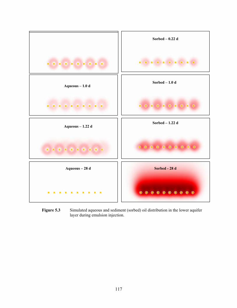
117

Figure 5.3 Simulated aqueous and sediment (sorbed) oil distribution in the lower aquifer layer during emulsion injection.

Sorbed – 1.0 d Aqueous – 1.0 d

Sorbed - 28 d

Sorbed – 0.22 d

Sorbed – 1.22 d

Aqueous – 0.22 d

Aqueous – 1.22 d

Aqueous – 28 d

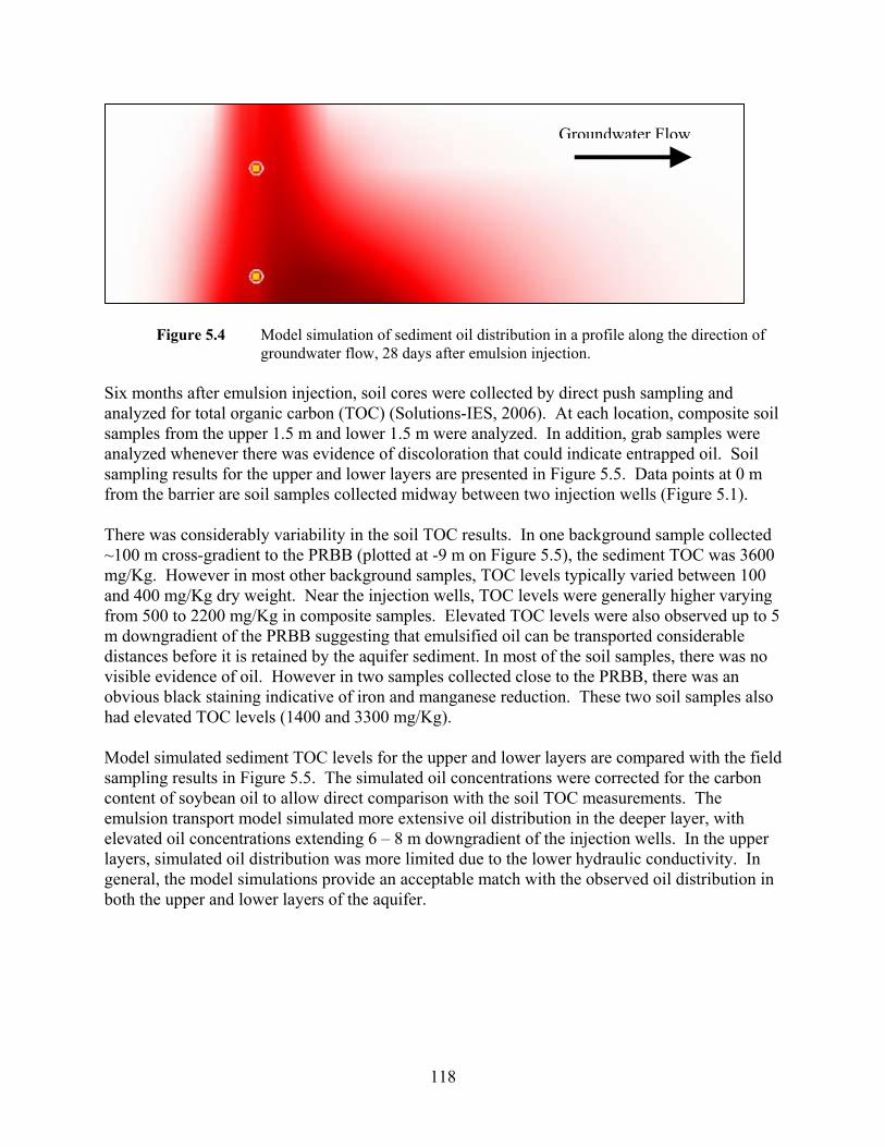
118

Figure 5.4 Model simulation of sediment oil distribution in a profile along the direction of groundwater flow, 28 days after emulsion injection.

Six months after emulsion injection, soil cores were collected by direct push sampling and analyzed for total organic carbon (TOC) (Solutions-IES, 2006). At each location, composite soil samples from the upper 1.5 m and lower 1.5 m were analyzed. In addition, grab samples were analyzed whenever there was evidence of discoloration that could indicate entrapped oil. Soil sampling results for the upper and lower layers are presented in Figure 5.5. Data points at 0 m from the barrier are soil samples collected midway between two injection wells (Figure 5.1). There was considerably variability in the soil TOC results. In one background sample collected ~100 m cross-gradient to the PRBB (plotted at -9 m on Figure 5.5), the sediment TOC was 3600 mg/Kg. However in most other background samples, TOC levels typically varied between 100 and 400 mg/Kg dry weight. Near the injection wells, TOC levels were generally higher varying from 500 to 2200 mg/Kg in composite samples. Elevated TOC levels were also observed up to 5 m downgradient of the PRBB suggesting that emulsified oil can be transported considerable distances before it is retained by the aquifer sediment. In most of the soil samples, there was no visible evidence of oil. However in two samples collected close to the PRBB, there was an obvious black staining indicative of iron and manganese reduction. These two soil samples also had elevated TOC levels (1400 and 3300 mg/Kg). Model simulated sediment TOC levels for the upper and lower layers are compared with the field sampling results in Figure 5.5. The simulated oil concentrations were corrected for the carbon content of soybean oil to allow direct comparison with the soil TOC measurements. The emulsion transport model simulated more extensive oil distribution in the deeper layer, with elevated oil concentrations extending 6 – 8 m downgradient of the injection wells. In the upper layers, simulated oil distribution was more limited due to the lower hydraulic conductivity. In general, the model simulations provide an acceptable match with the observed oil distribution in both the upper and lower layers of the aquifer.

Groundwater Flow

119

a. upper layer

0

500

1000

1500

2000

2500

3000

3500

4000

-10 -8 -6 -4 -2 0 2 4 6 8 10

Distance Downgradient from Barrier (m)

Soil

TO

C (m

g/K

g)

CompositeGrabModel-Shallow

b. lower layer

0

500

1000

1500

2000

2500

3000

3500

4000

-10 -8 -6 -4 -2 0 2 4 6 8 10

Distance Downgradient from Barrier (m)

Soil

TO

C (m

g/K

g)

CompositeGrabModel-deep

Figure 5.5 Comparison of simulated and observed sediment TOC in: (a) upper layer; and (b) lower layer.

5.4 MATHEMATICAL MODELING OF CONTAMINANT BIODEGRADATION Contaminant transport and biodegradation in the emulsified oil barrier and downgradient aquifer was simulated using the sequential decay model (Module # 6) within RT3D (Clement, 1997) where

120

( ) ASkAq

xvA

xAD

xtAR oilAs

sA −+

∂∂

−⎟⎠⎞

⎜⎝⎛

∂∂

∂∂

=∂∂

φ (1)

( ) ASkYBSkBq

xvB

xBD

xtBR oilAABoilBs

sB /+−+

∂∂

−⎟⎠⎞

⎜⎝⎛

∂∂

∂∂

=∂∂

φ (2)

( ) BSkYCSkCq

xvC

xCD

xtCR oilBBCoilCs

sC /+−+

∂∂

−⎟⎠⎞

⎜⎝⎛

∂∂

∂∂

=∂∂

φ (3)

( ) CSkYDSkDq

xvD

xDD

xtDR oilCCDoilDs

sD /+−+

∂∂

−⎟⎠⎞

⎜⎝⎛

∂∂

∂∂

=∂∂

φ (4)

and AA = aqueous phase concentration (moles / L) for compound A RA = retardation factor for compound A D = dispersion coefficient (m/d2) v = velocity (m/d) φ = porosity (dimensionless) qs = volumetric water flux per volume of aquifer representing sources and sinks As = source/sink concentration (moles/L) for contaminant A Soil = sediment oil concentration (g oil / g sediment) \kA = effective 2nd order decay coefficient (g sediment / g oil - d) for contaminant A YB/A = degradation product yield coefficient (moles of B produced per mole of A degraded) The actual numerical simulations were conducted using GMS 6.0 (Brigham Young University, 2005) to aid in data entry and visualization of model output. Prior to simulating contaminant transport, MODFLOW (McDonald and Harbaugh, 1988) was calibrated to match conditions at the field site. The aquifer was represented as a two layer system with injection and monitor wells fully penetrating both the upper and lower layers. The lower layer was assumed to have a hydraulic conductivity (K) approximately five times the upper layer based on visual observations of soil cores, grain size analyses, and slug tests on selected wells. Effective porosity and dispersivity were estimated by matching model simulations to results from the non-reactive tracer tests. Model parameters are summarized in Tables 5.1 and 5.2. Following emulsion injection, K was assumed to be reduced by up to 77% due to clogging with accumulated biomass, gas bubbles and/or retained oil based permeability test results reported by Solutions-IES (2006). The reduction in K was assumed to be linearly proportional to retained oil concentration where

Kreduced = Kinitial * (1 – 0.77 *Soil/ Maximum Soil)

121

Oil concentration in the sediment (Soil) was determined from numerical simulations of oil droplet transport and retention presented in Section 5.3.2 and varied from a maximum value of 0.0026 g oil per g sediment adjoining the injection wells to zero in untreated areas.

122

Table 5.2 RT3D Model Calibration Parameters.

Partition

Coefficient (mL/g)

2nd Order Decay Rate

(g sediment / g oil – d)

Range of Apparent 1st Order

Decay Rate(d-1)

Degradation Product

Degradation Product

Yield Coefficient

(mole / mole)ClO4 0 310 0 – 0.81 none NA 1

PCE 1240 2 140 0 – 0.36 TCE 1

TCE 388 2 225 0 – 0.59 cis-DCE 1

cis-DCE 61 2 43 0 – 0.11 VC 1

VC 22 2 65 0 – 0.17 NA NA

TCA 310 3 132 0 – 0.34 DCA 1

DCA 62 3 128 0 – 0.33 CA 1

CA 27 3 42 0 – 0.11 NA NA 1 NA – not applicable 2 Soybean oil : water partition coefficient from Pfeiffer, 2003. 3 Octanol : water partition coefficient from Howard, 1990. RT3D was initially calibrated to simulate the transport and attenuation of perchlorate, chlorinated ethanes and chlorinated ethenes during the quasi-steady-state period from 4 to 18 months (133 to 560 days) after emulsion injection. Contaminant biodegradation was modeled as a second order process where the contaminant decay rate was assumed to be linearly proportional to both Soil and the contaminant concentration. Soil was determined from prior simulations of oil droplet transport and retention (Section 5.3.2) and assumed constant over the simulation period. The contaminant transport model was first calibrated to match the observed contaminant distribution prior to emulsion injection using specified concentration cells to define the upgradient boundary condition. Contaminant retardation factors were estimated based on published soybean oil-water and octanol-water partition coefficients (Table 5.5). As presented in Chapter 3, a linear-equilibrium partitioning approach provided good estimates of the retardation of PCE in abiotic laboratory columns treated with emulsified soybean oil (Long and Borden, 2006). Once boundary and initial conditions were defined, the model was calibrated by adjusting the second order degradation rate for each contaminant until the mean error between observed and simulated steady-state concentrations was less than 0.5% of the average concentration. Estimated second order degradation rates for each contaminant are shown in Table 5.2. Simulated steady-state and observed concentrations in monitor and injection wells are compared in Table 5.3 and Figure 5.6. Observed values are the average of measured concentrations in wells during the quasi-steady-state period (measurements at 133, 285, 348 and 560 days after

123

emulsion injection). No attempt was made to simulate contaminant biodegradation during the first 4 months after emulsion injection when geochemical conditions in the aquifer were changing rapidly and the microbial community was adapting to the presence of injected soybean oil. Once calibrated, the model was used to evaluate the effect of alternative barrier designs on chlorinated solvent treatment efficiency.

124

Table 5.3 Comparison of Observed (Obs) and Simulated (Sim) Contaminant Concentrations in Monitor and Injection Wells during the Steady-State Period from 4 to 18 Months.

ClO4

(µg/L) TCA (µM)

DCA (µM)

CA (µM)

PCE (µM)

TCE (µM)

cis-DCE (µM)

VC (µM) Well

Obs Sim Obs Sim Obs Sim Obs Sim Obs Sim Obs Sim Obs Sim Obs Sim SMW-1 10633 9077 55.0 56.0 0.2 0.7 0.0 0.0 0.14 0.15 2.03 2.03 0.14 0.14 0.00 0.00SMW-2 8733 8036 57.4 57.4 0.5 0.5 0.1 0.1 0.28 0.28 1.41 1.41 0.11 0.11 0.01 0.00SMW-3 4633 5638 28.2 38.1 0.1 0.2 0.0 0.0 0.21 0.21 0.97 0.97 0.06 0.06 0.00 0.00SWM-4 4 7 9.7 1.8 10.1 5.4 11.4 23.4 0.03 0.01 0.15 0.02 0.65 0.59 0.00 0.44SMW-5 4.1 1 3.2 0.63 6.9 2.7 58.4 20.2 0.00 0.00 0.00 0.00 1.14 0.51 2.04 0.47SMW-6 5 1 2.7 0.61 9.4 2.7 17.0 20.1 0.04 0.00 0.06 0.00 0.63 0.44 0.00 0.40SMW-7 4 0 17.0 0.61 21.0 2.7 20.7 20.2 0.11 0.00 0.10 0.00 0.83 0.42 0.00 0.38IW-1 3333 1491 13.7 21.4 5.6 18.1 4.4 13.2 0.00 0.05 0.59 0.49 0.68 1.34 0.17 0.30IW-3 4 1300 8.9 22.1 16.3 18.7 19.6 13.7 0.03 0.07 0.16 0.47 1.37 1.27 0.46 0.29IW-5 409 1238 10.0 21.9 4.1 18.7 9.7 13.8 0.02 0.10 0.33 0.38 0.67 1.01 0.21 0.23IW-7 373 831 23.6 21.4 8.9 18.6 3.1 14.2 0.08 0.10 0.12 0.37 0.35 1.00 0.00 0.23IW-10 172 735 30.0 17.1 21.3 15.5 6.6 12.5 0.09 0.07 0.44 0.24 0.95 0.70 0.00 0.17Correlation Coefficient 0.97 0.88 0.33 0.59 0.86 0.97 0.59 0.44 Mean Error 5 -0.02 0.01 0.03 0.00 0.00 0.00 0.00 RMSE 963 9.1 8.8 12.6 0.05 0.14 0.37 0.51

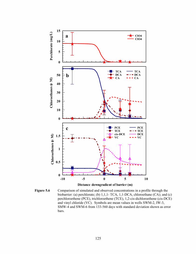
125

0

5

10

15

Perc

hlor

ate

(mg/

L)

ClO4ClO4

-10 -5 0 5 10

Distance downgradient of barrier (m)

0

0.5

1

1.5

Chl

oroe

then

es (μ

M)

PCETCEcis-DCEVC

PCETCEDCEVC

0

10

20

30

40

50

Chl

oroe

than

es (μ

M)

TCADCACA

TCADCACA

a

b

c

Figure 5.6 Comparison of simulated and observed concentrations in a profile through the

biobarrier: (a) perchlorate; (b) 1,1,1- TCA, 1,1-DCA, chloroethane (CA); and (c) perchloroethene (PCE), trichloroethene (TCE), 1,2-cis-dichloroethene (cis-DCE) and vinyl chloride (VC). Symbols are mean values in wells SWM-2, IW-3, SMW-4 and SWM-6 from 133-560 days with standard deviation shown as error bars.

126

5.4.1 Steady-State Simulations 5.4.1.1 Permeability Effects Simulated groundwater flow vectors in the region surrounding the emulsified oil biobarrier are shown in Figure 5.7a. Simulated flow vectors prior to emulsion injection are shown in Figure 5.7b for comparison. Prior to emulsion injection, groundwater flow is 1-D and perpendicular to the line of wells used to form the biobarrier. After emulsion injection, there is some flow around the barrier due to the reduced K in areas with retained oil. However, the effects on groundwater flow are not dramatic and groundwater velocity through the center of the barrier is only reduced by 31%. 5.4.1.2 Perchlorate The ClO4 distribution in groundwater nine months after EOS® injection (Solutions-IES (2006) is compared with the simulated ClO4 distribution in Figure 5.8a and 5.8b). The simulated perchlorate distribution was generated using an effective 2nd order degradation rate of 310 g sediment / g oil * d. This is equivalent to simulating perchlorate degradation with a 1st order decay approach where the apparent 1st order decay is linearly proportional to the sediment oil concentration and varies from 0.81 d-1 immediately adjoining the injection wells where the sediment oil concentration is highest to 0 d-1 in untreated areas.

a. Variable K after Emulsion Injection

127

Figure 5.7 Effect of reduced hydraulic conductivity (K) due to emulsion injection on simulated groundwater flow field: (a) postinjection – variable K distribution due to oil injection (reduced K zone is shaded); and (b) preinjection – uniform K distribution.

b. Uniform K before Emulsion Injection

128

1,000

10,000

100,000

<4

GroundwaterFlow

Direction

10,000 µg/L

100,000 µg/L

µg/L

µg/L

EOS® Injection Point

Groundwater Test Point

Figure 5.8 Comparisons of: a) measured ClO4 distribution in groundwater nine months after

EOS® injection; and b) simulated ClO4 distribution with spatially variable hydraulic conductivity due to emulsion injection.

In general, the calibrated model closely matches the observed perchlorate distribution in the aquifer (Figure 5.6a and 5.8). Simulated perchlorate concentrations in the downgradient wells (SMW-4, SMW-6, SMW-7) vary from 1 to 7 µg/L (>99.9% reduction). Average observed perchlorate concentrations during the steady-state period (4-18 months) varied from 4 to 5 µg/L (>99.9% reduction). Simulated concentrations in the injection wells varied from <1 to 1500 µg/L compared to observed concentrations that varied from <4 to 3300 µg/L.

b. Simulated ClO4 Distribution

a. Measured ClO4 Distribution

129

5.4.1.3 Chlorinated Ethanes Figure 5.6b shows simulated and observed TCA, DCA and CA concentrations along a streamline passing through the center of the barrier. In general, the calibrated model provides a good description of the spatial distribution of TCA during transport through the oil treated zone. However, the model somewhat over-predicts the extent of TCA degradation. In downgradient monitor wells SMW-4, SWM-5, SMW-6 and SMW-7, observed TCA concentrations vary from 3 to 17 µM while simulated concentrations vary from 0.6 to 1.8 µM. The model reasonably simulates the overall spatial distribution of DCA with higher concentrations in the injection wells (Sim = 15-18 µM, Obs = 4-21 µM) and lower concentrations in the downgradient monitor wells (Sim = 2.7-5.4 µM, Obs = 7-21 µM). However, it was not possible to match observed concentrations in individual wells. This is primarily due to the transient nature of this contaminant; DCA produced from TCA and then rapidly degraded to CA in the emulsion treated zone. During initial attempts to calibrate the model, CA degradation was assumed to occur only through abiotic hydrolysis with a spatially uniform 1st order decay rate of 0.016 d-1 (McCarty, 1996). However, it was not possible to obtain an adequate match between simulated and observed CA concentrations using this approach. Simulate CA concentrations were much higher than observed concentrations in both the injection and downgradient monitoring wells indicating that CA degradation was more rapid than could be explained by abiotic hydrolysis alone. Based on these results, CA degradation was assumed to occur through a biologically mediated reduction process, similar to TCA and DCA degradation. Assuming a second order CA degradation rate of 42 g sediment / g oil * d the model provides a reasonable match to the observed CA concentrations in the injection wells (Sim = 12.5-14.2 µM, Obs = 3-20 µM) and lower concentrations in the downgradient monitor wells (Sim = 20.1-23.4 µM, Obs = 11-58 µM). 5.4.1.4 Chlorinated Ethenes Figure 5.6c shows simulated and observed PCE, TCE, cis-DCE and VC concentrations along a streamline passing through the center of the barrier. The calibrated model provides a good description of the spatial distribution of PCE, TCE and cis-DCE during transport through the oil treated zone. However, the model was not able to match the observed spatial variation in VC in the downgradient monitor wells. VC concentrations were extremely variable in wells located 6 m downgradient of the barrier ranging from 2.0 µM in SMW-5 to below detection in SWM-6 and SMW-7. There is no apparent reason for this large variation VC concentrations, and not surprisingly, simulated VC were relatively uniform (0.38 – 0.47 µM). The maximum apparent first order decay rates ranged from 0.59 d-1 for TCE to 0.11 d-1 for cis-DCE. These rates are generally consistent with values previously reported for enhanced anaerobic bioremediation systems (Suarez and Rifai, 1999).

130

5.4.2 Full Scale Barrier Performance Once calibrated, the model was used to evaluate two different barrier alternatives. For both alternatives, a 10 m wide portion of the barrier was simulated with the model domain extending 15 m upgradient of the barrier and 30 m downgradient. Since only a short section of barrier was simulated, upgradient contaminant concentrations were assumed to be uniform and equal to 9,000 µg/L ClO4, 57.4 µM TCA, 0.5 µM DCA, 0.08 µM CA, 0.26 µM PCE, 1.41 µM TCE, 0.11 µM cis-DCE, and 0 µM VC. The hydraulic gradient was 0.005. All other model parameters were identical to those used in prior simulations (Tables 5.1 and 5.2). For Barrier Alternative I, injection wells were spaced 5 m apart, perpendicular to groundwater flow with continuous screens extending through both the upper and lower layers. A 20% EOS: 80% water solution was injected in every other well for 0.5 days followed by chase water for 1.5 days. This procedure was then repeated with the remaining wells. The emulsion and chase water injection flow rate was 4 m3/d per well to match the flow rate previously used in the field. The flow rate entering each layer was assumed to be proportional to the layer transmissivity with 16% of the flow entering the upper, less permeable layer (K=2.1 m/d) and 84% of the flow entering the lower, more permeable layer (K=10.7 m/d). Figure 5.9 shows the simulated oil distribution in the sediment following injection and the steady-state aqueous contaminant distributions for Barrier Alternative I. In the lower layer, oil is effectively distributed between the injection wells resulting in a relatively uniform oil treated zone 13-18 m long along the direction of groundwater flow with a hydraulic retention time (HRT) of 3 - 4 months. The relatively high residual oil concentrations without this zone (0.0037 g/g) combined with the large HRT results in very high treatment efficiencies in the lower layer, with all contaminants reduced below applicable regulatory standards. However in the upper layer, the oil distribution is much less uniform varying from 0.0037 g/g near the injection wells to 0.00033 g/g midway between the injection wells. This non-uniform oil distribution allows large amounts of contaminants to pass untreated through the gaps in the oil treated zone. Farther downgradient, residual contaminants diffuse from the upper layer into the lower layer. Barrier Alternative II uses one set of continuously screened injection wells spaced 5 m apart (same as Alternative I) with a second set of injection wells located midway between the 1st set and screened only in the upper, lower permeability layer. The injection process for the 1st set of wells is identical to Alternative I. Once the 1st set of injections is complete, a 20% EOS: 80% water solution is injected into the 2nd set of wells for 0.5 days followed by chase water for 1.5 days at a flow rate of 0.66 m3/d per well.

131

Figure 5.10 shows the simulated oil distribution in the sediment following injection and the steady-state aqueous contaminant distributions for Barrier Alternative II. The modified injection procedure followed in Alternative II results in continuous oil treated zones in both the upper and lower layers. The zones of high oil residual saturation (~ 0.0037 g/g) are 5-6 m long in the upper layer and 13-17 m long in the lower layer with HRT’s that vary from 4-5 months in the upper zone to 3 – 4 months in the lower zone. The long contact time between the contaminants and oil in both the upper and lower layers results in very effective treatment, with all contaminants reduced below treatment standards in both the upper and lower layers.

132

Oil ClO4 TCA DCA CA PCE TCE cis-DCE VC (g/g) (µg/L) (µM) (µM) (µM) (µM) (µM) (µM) (µM)

Figure 5.9 Oil distribution in sediment following injection and steady-state aqueous contaminant distribution for Barrier Alternative I.

Low

er L

ayer

U

pper

Lay

er

133

Oil ClO4 TCA DCA CA PCE TCE cis-DCE VC (g/g) (µg/L) (µM) (µM) (µM) (µM) (µM) (µM) (µM)

Figure 5.10 Oil distribution in sediment following injection and steady-state aqueous contaminant distribution for Barrier Alternative II.

Low

er L

ayer

U

pper

Lay

er

134

5.5 SUMMARY A permeable reactive biobarrier (PRBB) was installed to enhance in-situ anaerobic biodegradation of perchlorate and chlorinated solvents. The PRBB was installed by injecting 420 L of soybean oil-in-water emulsion through ten direct push injection wells over a two day period. Soil cores collected six months after emulsion injection indicate the oil was distributed up to 5 m downgradient of the injection wells. A previously developed model (Chapter 4) was then used to simulate emulsion transport at the field site. The model was first calibrated to simulate groundwater flow and solute transport using results from the field site characterization and a non-reactive tracer test. Emulsion transport parameters were estimated from a laboratory column test using aquifer material from the site. Emulsion retention was lower in this column test than in prior work, indicating emulsion transport may be more rapid at this site. While there was considerable variability in the soil sampling results, the model simulations generally agreed with the observed oil distribution at the field site. Contaminant transport and degradation within the biobarrier was simulated using the sequential decay module within RT3D. Contaminant biodegradation was modeled as a second order process where the contaminant decay rate was assumed to be linearly proportional to both the residual oil concentration and the contaminant concentration. Groundwater flow was simulated with MODFLOW where hydraulic conductivity was reduced by up to 77% in those areas with the highest oil concentration. Using this approach, the calibrated model was able to closely match the observed contaminant distribution. Maximum apparent first order decay rates varied 0.11 d-1 for cis-DCE and CA to 0.59 d-1 for TCE and 0.81 d-1 for ClO4. The calibrated model was then used to design a full-scale barrier to treat both ClO4 and chlorinated solvents. When emulsion was injected using continuously screened wells spaced 5 m on-center, gaps in the oil treated zone allowed some contaminants to escape downgradient untreated. However, use of continuously screened wells in combination with shorter wells only screened in the lower permeability zone resulted in a much more uniform oil distribution. Model simulations indicate that this alternative injection approach should result in excellent treatment with all contaminants reduced below treatment standards in both higher and lower permeability zones. 5.6 REFERENCES

Achenbach, L.A., Michaelidou, U., Bruce, R.A., Fryman, J., Coates, J.D., 2001. Dechloromonas

agitata gen. nov., sp. nov. and Dechlorosoma suillum gen. nov., sp. nov., two novel environmentally dominant (per)chlorate-reducing bacteria and their phylogenetic position,” International Journal of Systematic and Evolutionary Microbiology 51, 527–33.

AFCEE and NFESC, 2004. Principles and Practices of Enhanced Anaerobic Bioremediation of

Chlorinated Solvents, Air Force Center for Environmental Excellence, Brooks Air Force Base, Texas and Naval Facilities Engineering Service Center (NFESC), Port Hueneme, CA.

Borden, R.C., Rodriguez, B.X., 2006. Evaluation of slow release substrates for anaerobic

bioremediation, Bioremediation Journal, 10(1-2):56-69. Boulicault, K.J., Hinchee, R.E., Wiedemeier, T.H., Hoxworth, S.W., Swingle, T.P., Carver, E., Haas,

P.E., 2000. Vegoil: A novel approach for stimulating reductive dechlorination. In:

135

Wickramanayake, G.B., Gavaskar, A.R., Alleman, B.C., Magar, V.S. (Eds) Bioremediation and Phytoremediation of Chlorinated and Recalcitrant Compounds, Battelle Press. pp. 1-7.

Bouwer, H. Rice, R.C., 1976. A slug test method for determining hydraulic conductivity of

unconfined aquifers with completely or partially penetrating wells. Water Resources Research 12, 423-428.

Brigham Young University, 2005. The Department of Defense Groundwater Modeling System, GMS v6.0, Environmental Modeling Laboratory.

Chaudhuri, S.K., O’Connor, S.M., Gustavson, R.L., Achenbach, L.A., Coates, J.D., 2002.

Environmental factors that control microbial perchlorate reduction, Appl. Environ. Microbiol. 68, 4425-4430.

Clement, T.P., 1997. RT3D – A Modular Computer Code for Simulating Reactive Multi-Species

Transport in 3-Dimensional Groundwater Aquifers, Battelle Pacific Northwest National Laboratory Research Report, PNNL-SA-28967.

Clement, T.P., 1997. RT3D – A Modular Computer Code for Simulating Reactive Multi-Species

Transport in 3-Dimensional Groundwater Aquifers, Battelle Pacific Northwest National Laboratory Research Report, PNNL-SA-28967.

Coates, J.D., Michaelidou, U., Bruce, R.A., O’Connor, S.M., Crespi, J.N., Achenbach, L.A., 1999.

Ubiquity and diversity of dissimilatory (per)chlorate-reducing bacteria., Appl. Environ. Microbiol. 65, 5234-5241.

Coulibaly, K.M., Borden, R.C., 2004. Impact of edible oil injection on the permeability of aquifer

sands, J. Contaminant Hydrology, 71, 219-237. Groundwater Technology, Inc., 1990. Pre-Remediation Investigation, Incinerator Feed Surface

Impoundment. March 15, 1990. Hanaki, K, Nagase, M. Matsuo, T., 1981. Mechanism of inhibition caused by long-chain fatty acids in

anaerobic digester process. Biotech. Bioeng. 23, 1591-1610. Hatzinger, P.B., 2005. Perchlorate biodegradation for water treatment, Environ. Sci. Technol. 39,

239A–47A. Howard, P. H. 1990. Handbook of Environmental Fate and Exposure Data for Organic Chemicals.

Volume II. Solvents. Lewis Publishers, Chelsea, MI. Hunter, W.J., 2001. Use of vegetable oil in a pilot-scale denitrifying barrier, J. Cont. Hydro. 53, 119-

131. Hunter, W.J., 2002, Bioremediation of chlorate or perchlorate contaminated water using permeable

barriers containing vegetable oil, Current Microbiol., 45, 287-292. ITRC Perchlorate Team, 2005. Perchlorate: Overview of Issues, Status, and Remedial Options,

Interstate Technology & Regulatory Council, Washington, DC .

136

Lee, M.D., Odom, J.M., Buchanan, R. J., 1998. New perspectives on microbial dehalogenation of

chlorinated solvents: insights from the field, Ann. Rev. Microbiol. 52, 423-452. Lee, M. D., Lieberman T.M., Borden R.C., Beckwith W., Crotwell T. and Haas P.E., 2001. Effective

distribution of edible oils – results from five field applications. In: Wickramanayake, G.B., Gavaskar, A.R., Alleman, B.C., Magar, V.S. (Eds.), Proc. In Situ and On-Site Bioremediation: The Sixth Internal. Sym., San Diego, CA, Battelle Press, Columbus, OH.

Lee, M.D., Lieberman, M.T., Beckwith, W.J., Borden, R.C., Everett, J., Kennedy, L., Gonzales, J.R.,

2003. Pilots to enhance trichloroethene reductive dechlorination and ferrous sulfide abiotic transformation, Paper K-14, In: V.S. Magar and M.E. Kelley (Eds.), Proceedings of the Seventh International In Situ and On-Site Bioremediation Symposium (Orlando, FL). ISBN 1-57477-139-6, Battelle Press, Columbus, OH.

Lindow, N.L, Borden, R.C., 2005. Anaerobic bioremediation of acid mine drainage using emulsified

soybean oil, Mine Water and the Environment 24, 199–208. Lindow, N.L., 2004. Use of Soybean Oil and Soybean Products for Groundwater Bioremediation,

Master of Science Thesis, North Carolina State University, Raleigh, NC. Long, C. M., and R. C. Borden, 2006. Enhanced Reductive Dechlorination in Columns Treated with

Edible Oil Emulsion, J. Contaminant Hydrology, 87: 54–72. Logan, B.E., 1998. A review of chlorate- and perchlorate-respiring microorganisms, Bioremediation

Journal 2: 69–79. Logan, B.E., 2001, Assessing the outlook for perchlorate remediation, Environ. Sci. & Technol.: 35,

482A- 487A. Major, D.W., McMaster, M.L, Cox, E.E., Edwards, E.A., Dworatzek, S.M., Hendrickson, E.R., Starr,

M.G., Payne, J.A., Buonamici, L.W., 2002. Field demonstration of successful bioaugmentation to achieve dechlorination of tetrachloroethene to ethene, Environ. Sci. Technol. 36, 5106-5116.

May, I., Panhorst, E.M, Page, G.B, Sgambat, J.P, Lutes, C.C., Suthersan, S.S., 2004. In situ field

testing for RDX/TNT in groundwater using enhanced anaerobic bioremediation. Proceedings of the Conference on Sustainable Range Management, New Orleans, Louisiana: January 5 - 8.

McCarty, P.L., 1996. Biotic and abiotic transformations of chlorinated solvents in ground water.

Symposium on the Natural Attenuation of Chlorinated Organics in Ground Water, EPA/540/R-96/509, U.S. Environmental Protection Agency, Washington, D. C., 5-9.

McCarty, P.L., Semprini, L., 1994. Ground-water treatment for chlorinated solvents, In: Norris, R.D.,

Hinchee, R.E., Brown, R., McCarty, P.L, Semprini, L., Wilson, J.T., Kampbell, D.H., Reinhard, M., Bouwer, E.J., Borden, R.C., Vogel, T.M., Thomas, J.M., and Ward, C.H., (Eds.) Handbook of Bioremediation, Lewis Publishers, Boca Raton, FL, p. 87–116.

137

McDonald, J. M., Harbaugh, A.W., 1988. A modular three-dimensional finite-difference groundwater flow model. Techniques of water resources investigations of the U.S. Geological Survey Book 6.

Nevin, K.P., Finneran, K.T., and Lovley, D.R., 2003. Microorganisms associated with uranium

bioremediation in a high-salinity subsurface sediment, Appl. Envir. Micro., 69, 3672-3675. Pfeiffer, P., 2003. Abiotic Effects of Vegetable Oil Added to Enhance In-Situ Bioremediation of

Chlorinated Solvents. Masters of Science Thesis, University of Colorado, Boulder, CO. Ralston, A.W., Hoerr, C.W., 1942. The solubilities of the normal saturated fatty acids, J. Org. Chem.

7, 546-555. Rikken, G.B., Kroon, A.G.M., van Ginkel, C.G., 1996. Transformation of (per)chlorate into chloride

by a newly isolated bacterium: reduction and dismutation, Appl. Micrbiol. Biotechnol. 45, 420-426.

Sawyer, C.N., McCarty, P.L., Parkin, G.F., 1994. Chemistry for Environmental Engineering. McGraw-

Hill Inc. Solutions-IES, 2006. Edible Oil Barriers for Treatment of Perchlorate Contaminated Groundwater,

Environmental Security and Technology Certification Program, Arlington, VA (www.estcp.org).

Suarez, M. P., Rifai, H.S., 1999. Biodegradation Rates for Fuel Hydrocarbons and Chlorinated

Solvents in Groundwater, Bioremediation J., 3(4):337 – 362. Sun, B., Griffin, B.M, Ayala-del-Rio, H.L., Hashshman, S.A., Tiedje, J.M., 2002. Microbial

dehalorespiration with 1,1,1-trichloroethane. Science 298, 1023-1025. Vogel, T.M., Criddle, C.S., McCarty, P.L., 1987. Transformations of halogenated aliphatic

compounds, Environ. Sci. Technol., 21, 722-736. Vogel, T.M., McCarty, P.L., 1987. Abiotic and Biotic transformations of 1,1,1-trichloroethane under

methanogenic conditions, Environ. Sci. Technol., 21, 1208-1213. Waller, A.S., Cox, E.E., Edwards, E.A., 2004. Perchlorate-reducing microorganisms isolated from

contaminated sites, Environmental Microbiology 6, 517–27. Xu, J.Y., Song, Y., Min, B., Steinberg, L., Logan, B.E., 2003. Microbial degradation of perchlorate:

principles and applications, Environmental Engineering Science 20, 405– 22. Zenker, M.J., Borden, R.C., Barlaz, M.A., Lieberman, M.T., Lee, M.D., 2000. Insoluble substrates for

reductive dehalogenation in permeable reactive barriers. In: Wickranayake, G.B., Gavaskar, A.R., Alleman, B.C., Magar, V.S. (Eds.), Bioremediation and Phytoremediation of Chlorinated and Recalcitrant Compounds. pp 77 - 84. Battelle Press. Columbus, OH.

Zhang, H., Bruns, M.A., Logan, B.E., 2002. Perchlorate reduction by a novel chemolithoautotrophic, hydrogen-oxidizing bacterium, Environmental Microbiology 4, 570–76.

138

Zheng, C., 1990. MT3D - A Modular Three-Dimensional Transport Model for Simulation of

Advection, Dispersion and Chemical Reactions of Contaminants in Groundwater System. U.S. Environmental Protection Agency, Ada, OK.

139

CHAPTER 6: CONCLUSIONS

At the start of this project, neat and emulsified vegetable oil had been used at several different sites to simulate anaerobic biodegradation of chlorinated solvents and other contaminants in groundwater. However, little was known about the transport, retention and biodegradation of these materials in the subsurface or the impact of these materials on contaminant fate. This project included a series of laboratory, field and numerical modeling studies aimed at improving our understanding of edible oil transport and fate in the subsurface. This information was then used to develop an effective process for enhancing in situ anaerobic biodegradation of ground water contaminants. Edible Oil Transport and Retention in Laboratory Columns Laboratory studies were first conducted to develop methods for distributing edible oils away from the point of injection and to evaluate the effect of the injection method on aquifer permeability. Laboratory columns packed with sands or clayey sands were flushed with either neat oil or a soybean emulsion followed by plain water, while permeability loss and the final oil residual saturation were monitored. Neat soybean oil could be distributed short distances in laboratory columns packed with sand without excessive permeability loss if the oil was be displaced to residual saturation. However in the field, oil displacement to residual saturation would likely be very difficult because of the high viscosity of the soybean oil and the large volumes of injection water required. If the oil is not displaced to residual saturation, permeability losses will be much greater and there is potential for upward migration of the oil due to buoyancy effects. Injection of edible oil-in-water emulsions appears to offer many advantages over injection of neat oil. Soybean oil-in-water emulsions can be prepared using only food-grade, Generally Recognized As Safe (GRAS) materials to aid in gaining regulatory approval. Using appropriate combinations of surfactants and high-energy mixers, emulsions with very small droplets can be prepared that will easily pass through the pores of most sandy sediments. For the fine emulsions used in this study, the primary mechanism of oil retention is believed to be interception, where oil droplets collide with pore surfaces and stick. Retention of these emulsions was very low in pure sand and increased linearly with clay content. Emulsion injection did result in some permeability loss. However for sands with low to moderate clay content, the permeability loss is modest (0 to 40% loss) and is proportional to the oil residual saturation. Results of this work indicate that appropriately prepared emulsions can be distributed in representative aquifer material without excessive permeability loss, and suggests that edible oil emulsions can potentially be used to form biologically active permeable reactive barriers. Impact of Edible Oil Emulsions on Chlorinated Solvent Transport and Biodegradation In this work, we evaluated the effects of emulsified soybean oil addition on reductive dechlorination of PCE in laboratory columns packed with fine clayey sand. Concentrations of chlorinated solvents, electron acceptors, donors and indicator parameters were monitored to evaluate reductive dechlorination efficiency and estimate carbon usage over time. Head loss was monitored to evaluate the effect of emulsion addition on permeability loss. Subsequent laboratory studies were then conducted to identify alternative substrates that would support reductive dechlorination and be even more long-lasting than soybean oil. Experimental results from this work have shown that a single injection of emulsified soybean oil can be effective in enhancing reductive dechlorination. However, a

140

number of important issues were identified related to the design and performance of full-scale edible oil barriers. • Soybean oil emulsion was effective in enhancing reduction of PCE to cis-DCE. However, yeast

extract addition was required to stimulate rapid growth of microorganisms that can reduce cis-DCE to ethene. These results suggest that inorganic nutrients, vitamins, amino acids or other materials present in yeast extract, but absent from soybean oil, may be required for effective growth of microorganisms that can dechlorinate cis-DCE to VC and ethene.

• Emulsified soybean oil can provide a long-term source of organic carbon to support anaerobic

biodegradation processes. A single injection of emulsified soybean oil supported reductive dechlorination in laboratory columns for over 14 months. Mass balance results indicated that the injected substrate would be completely depleted in 6 to 7 years. However, pollutant removal efficiency can be expected to decline before the injected carbon is completely depleted, requiring the injection of additional emulsion to maintain performance.

• Emulsified soybean oil is an effective substrate for stimulating reductive dechlorination.

However, chlorinated solvent biodegradation rates may be somewhat lower than when using soluble materials (e.g. lactate or yeast extract) as the carbon source. The potential impacts of somewhat slower biodegradation rates need to be considered when designing an emulsified oil barrier. In the field, it may be desirable to generate emulsion treated zones that provide at least a 30 day contact time between the chlorinated solvent and emulsion treated aquifer material.

• Emulsified oil injection will increase the organic carbon content near the point of injection,

increasing the apparent sorption of chlorinated solvents to the emulsion treated aquifer material. The laboratory column studies indicate that the effect of retained soybean oil on contaminant migration sorption can be reasonably approximated using a linear, equilibrium, retardation approach. In the absence of biological activity, transport of hydrophobic contaminants can be significantly delayed by sorption to the oil. However in practice, the more highly chlorinated ethenes (e.g. PCE and TCE) are rapidly transformed to more soluble daughter products which do not strongly sorb to the retained oil.

• In the absence of biological activity, properly prepared edible oil emulsions do not result in

significant permeability loss. However, the enhanced biological activity associated with emulsion injection can result in significant biomass production and/or gas bubble accumulation, with a resulting decline in permeability. Permeability losses in the emulsion treated columns were less than in a parallel column receiving soluble substrates (lactate and yeast extract). Regardless of the substrate used, the effects of biological activity on aquifer permeability need to be carefully considered when planning an enhanced anaerobic bioremediation project.

• In addition to soybean oil, there are a wide variety of lower solubility organic substrates that

could be used in emulsified oil barriers (e.g. including fatty acids, surfactants, fats and oils, and sucrose esters of fatty acids). The large majority of these materials can be fermented to carbon dioxide and methane indicating they can also provide H2 and acetate to support reductive dechlorination. It should be possible to reduce the required frequency for substrate injection by using a more slowly biodegradable substrate. However, using a more slowly biodegradable

141

substrate is also expected to reduce the contaminant biodegradation rate, requiring a biobarrier with a longer contact time to achieve target treatment efficiencies. In practice, it may be less expensive to use a moderately biodegradable substrate (e.g. soybean oil) and periodically reinject.

Laboratory Studies of Emulsified Oil Transport and Retention

To provide effective treatment, emulsified oils must be brought into close contact with the contaminant. This requires distributing the emulsified oil out away from the injection point. 1-D column experiments and 3-D radial flow sandbox experiments were conducted to gain a better understanding of the processes controlling emulsified oil transport in the subsurface and develop a numerical model that could be used in the design of emulsified oil injection project. • Results from laboratory column experiments demonstrated that appropriately prepared soybean

oil-in-water emulsions can be distributed in clayey sand at least 80 cm away from injection point. Kaolinite addition to the clayey sand resulted in an increase in the maximum oil retention.

• A reaction module for the numerical model RT3D was developed to simulate emulsion

transport and retention. This module is based on standard colloidal transport theory with a Langmuirian blocking function to account for saturation of attachment site with retained oil droplets. This model provided an adequate description of effluent breakthrough and the final oil distribution in the laboratory columns.

• Injection of a fine emulsion followed by chase water was very effective in distributing oil

throughout a 1.2 m x 0.98 m x 0.98 m 3-D sandbox. Samples collected approximately two months after injection showed that organic concentrations were reasonably uniform with depth, indicating the oil did not float upward after the end of injection.

• The emulsion transport model described above was calibrated using independently measured

transport parameters and successfully predicted the final oil distribution in both homogeneous and heterogeneous sandbox experiments. The good match between predicted and observed values indicates the validated model can be used to describe the transport and distribution of emulsified oil in sandy sediments.

Field Studies of Emulsified Oil Transport and Contaminant Biodegradation

A detailed field pilot test was conducted to evaluate the use of an emulsified oil biobarrier to enhance the in-situ anaerobic biodegradation of perchlorate and chlorinated solvents in groundwater. The biobarrier was installed by injecting 380 L of commercially available soybean oil-in-water emulsion through ten direct push injection wells over a two day period. • Soil cores collected six months after emulsion injection indicate the oil was distributed up to 5

m downgradient of the injection wells.

142

• A previously developed emulsion transport model was used to simulate emulsion transport and

retention using independently estimated model parameters. While there was considerable variability in the soil sampling results, the model simulations generally agreed with the observed oil distribution at the field site.

• Field monitoring results over a 2.5 year period following emulsion injection indicates the oil

injection generated strongly reducing conditions in the oil treated zone with depletion of dissolved oxygen, nitrate, and sulfate, and increases in dissolved iron, manganese and methane. Perchlorate was degraded from 3,100 – 20,000 µg/L to below detection (<4 µg/L) in the injection and nearby monitor wells within 5 days of injection. Two years after the single emulsion injection, perchlorate was less than 6 µg/L in downgradient wells compared to an average upgradient concentration of 13,100 µg/L.

• Emulsion injection stimulated reductive dechlorination of 1,1,1-TCA, PCE and TCE during

groundwater migration through the biobarrier. However, these compounds were not reduced to target treatment levels and appreciable levels of degradation products (e.g. cis-DCE, 1,2-DCA and CA) remained downgradient of the biobarrier . The incomplete removal of TCA, PCE and TCE is likely associated with the short (5 – 20 day) hydraulic retention time of contaminants in the emulsion treated zone.

• Emulsion injection did result in some permeability loss presumably due to biomass growth

and/or gas production. However, non-reactive tracer tests and detailed monitoring of the perchlorate plume demonstrated that the permeability loss did not result in excessive flow by-passing around the biobarrier.

• Contaminant transport and degradation within the biobarrier was simulated using RT3D where

biodegradation rate was assumed to be linearly proportional to the residual oil concentration and the contaminant concentration. Using this approach, the calibrated model was able to closely match the observed contaminant distribution. The calibrated model was then used to design a full-scale barrier expected to meet remediation objectives for both ClO4 and chlorinated solvents.

Research Needs Enhanced anaerobic bioremediation could potentially be used to treat source areas contaminated with dense non-aqueous phase liquids (DNAPLs). However, DNAPL bioremediation can be challenging because of the difficulties associated with distributing readily biodegradable soluble substrates. Sleep et al. (Environ. Sci. Tech. 40: 3623-3633, 2006) found that injection of soluble substrate initially stimulated PCE biotransformation in a 2-D sandbox containing residual DNAPL. However, reductive dechlorination declined with time as the injected substrate was fermented to methane before it reached the DNAPL. This occurred, even though a substantial portion of the original PCE was still present in the sandbox. In contrast, Yang and McCarty (Environ. Sci. Tech. 36: 3400-3404, 2002) showed that vegetable oil mixed PCE DNAPL was an excellent substrate for enhancing reductive dechlorination. The key challenge is to develop an effective approach for contacting vegetable oil with DNAPL. Currently, we have a very poor understanding of how emulsified oils interact with DNAPLs and how

143

mixtures of these materials biodegrade. Additional research is needed to understand these interactions and develop effective delivery approaches. Over the course of this project, we developed and demonstrated methods for distributing small particles (e.g. oil droplets) in aquifers to stimulate anaerobic biodegradation. This general approach should also be applicable to distribution of other solid and liquid materials. However, additional research will be needed to understand the different factors controlling the transport and longevity of these materials in the subsurface.

APPENDIX A LIST OF TECHNICAL PUBLICATIONS

Appendix A List of Technical Publications

Theses and Dissertations Jung, Y., MS Thesis, Transport of Emulsified Edible Oil in a 3-Dimensional Sandbox: Experimental

and Modeling Results, North Carolina State University, Raleigh, NC, June 2003. Long, C. M., MS Thesis, Enhanced Reductive Dechlorination in Edible Oil Barriers – Experimental

and Modeling Results, North Carolina State University, Raleigh, NC, August 2004. Rodriguez, B. X., MS Thesis, Evaluation of Slow Release Substrates for Anaerobic Bioremediation,

North Carolina State University, Raleigh, NC, August 2004. Coulibaly, K. M., PhD Dissertation-Geology, Permeability Reduction and Emulsified Soybean Oil

Distribution in Aquifer Sediments: Experimental and Modeling Results, North Carolina State University, Raleigh, NC, December 2004.

Journal Articles Coulibaly, K.M., and R.C. Borden, Impact of Edible Oil Injection on the Permeability of Aquifer

Sands, J. Contaminant Hydrology, 71(1-4):219-237, 2004. Coulibaly, K.M., C.M. Long, and R.C. Borden, Transport of Edible Oil Emulsions in Clayey-Sands: 1-

D Column Results and Model Development, J. Hydrologic Engr. 11(3):230-237, 2006. Jung, Y., K.M. Coulibaly, and R.C. Borden, Transport of Edible Oil Emulsions in Clayey-Sands: 3-D

Sandbox Results and Model Validation, J. Hydrologic Engr. 11(3):238-244, 2006. Long, C.M., and R.C. Borden, Enhanced Reductive Dechlorination in Columns Treated with Edible

Oil Emulsion, J. Contaminant Hydrology, 87: 54–72, 2006. Borden, R.C. and B. Ximena Rodriguez, Evaluation of Slow Release Substrates for Anaerobic

Bioremediation , Bioremediation Journal, 10(1–2):59–69, 2006 Borden, R.C., Anaerobic Bioremediation of Perchlorate and 1,1,1-Trichloroethane in an Emulsified Oil

Barrier, Journal of Contaminant Hydrology, accepted for publication. Borden, R.C., Effective Distribution of Emulsified Edible Oil for Enhanced Anaerobic Bioremediation,

Journal of Contaminant Hydrology, accepted for publication. Symposium and Conference Proceedings Jung, Y. and R.C. Borden, Subsurface Transport of Emulsified Edible Oil – 3-D Sandbox and

Modeling Results, Paper B-11, In: V.S. Magar and M.E. Kelley (Eds.), Proceedings of the Seventh International In Situ and On-Site Bioremediation Symposium (Orlando, FL; June 2003). ISBN 1-57477-139-6, Battelle Press, Columbus, OH.

Coulibaly, K.M. and R.C. Borden, Distribution of Edible Oil Emulsions and Permeability Loss in Sandy Sediments, Paper B-10, In: V.S. Magar and M.E. Kelley (Eds.), Proceedings of the Seventh International In Situ and On-Site Bioremediation Symposium (Orlando, FL; June 2003). ISBN 1-57477-139-6, Battelle Press, Columbus, OH.

Borden R.C., K.M. Coulibaly, Y. Jung, C.M. Long, N.L. Lindow, M.D. Lee, M.T. Lieberman, J.R.

Gonzales. Use of Edible Oil Substrate (EOS®) for In Situ Anaerobic Bioremediation, Air Force Center for Environmental Excellence Annual Workshop, San Antonio, TX, 2003.

Symposium and Conference Presentations and Posters Edible Oil Barriers for Enhanced Anaerobic Biodegradation of Chlorinated Solvents, Partners in

Environmental Technology Technical Symposium & Workshop; Arlington, VA, 2000 (poster). Enhanced Anaerobic Bioremediation using Emulsified Edible Oils, Partners in Environmental

Technology Symposium & Workshop, SERDP, Alexandria, VA, Nov. 2001 (poster). In-Situ Anaerobic Bioremediation using Emulsified Edible Oils, Partners in Environmental

Technology Symposium & Workshop, SERDP, Alexandria, VA, Dec. 2002 (poster). Anaerobic Biodegradation of Perchlorate and TCA in an EOS® Permeable Reactive Barrier, Partners

in Environmental Technology Symposium & Workshop, SERDP, Washington, DC, Dec. 2004 (poster).

Potential for using Edible Oil Emulsion for Remediation of Chlorinated Solvent Contamination in a

Source Area, Partners in Environmental Technology Symposium & Workshop, SERDP, Washington, DC, Dec. 2004 (poster).

Enhanced Anaerobic Bioremediation of Perchlorate and Chlorinated Solvents Using Emulsified Oil

Substrate, Partners in Environmental Technology Symposium & Workshop, SERDP, Washington, DC, Dec. 2005 (poster).

Use of Emulsified Edible Oil for In-Situ Anaerobic Bioremediation, In Situ and On-Site

Bioremediation: The Seventh International Symposium, Orlando, FL, 2003 (platform). Reductive Dechlorination in Edible Oil Barriers – Experimental and Modeling Results, Proc. In Situ

and On-Site Bioremediation: The Seventh International Symposium, Orlando, FL, 2003 (platform).

Treatment of Perchlorate and 1,1,1-Trichloroethane in Groundwater using Edible Oil Substrate

(EOS®), Proceedings of Remediation of Chlorinated and Recalcitrant Compounds – 4th Internat. Conf., May 2004.

Guidelines for Effective Distribution of Emulsified Edible Oils, Proc. Remediation of Chlorinated and

Recalcitrant Compounds – 4th Internat. Conf., May 2004.

Remediation of Perchlorate and Trichloroethane in Groundwater Using Edible Oil Substrate (EOS®), National Ground Water Association Conference on MTBE and Perchlorate: Assessment, Remediation and Public Policy, Costa Mesa, CA, June, 2004 (platform).

Anaerobic Bioremediation with EOS® – Cost Effective Design and Field Implementation, In Situ and

On-Site Bioremediation: The Eighth Seventh International Symposium, Baltimore, MD, June 2005 (platform).

in-situ permeable barriers for reductive dehalogenation of

Documents