in teractiv e r ay t racin g o f n u r b s s u rfaces b y...
TRANSCRIPT

Interactive Ray Tracing of NURBSSurfaces by Using SIMD Instructions
and the GPU in Parallel
Diploma Thesis
Presented by
Oliver P. Abert
Centre for Graphics and Media TechnologyNanyang Technological University
Institute for Computational VisualisticsWorking Group Computer Graphics
Examiner: Prof. Dr.-Ing. Stefan Müller2nd Examiner: Assoc. Prof. Dr. Ing. Wolfgang Müller
September 2005


Eidesstattliche Erklärung
Hiermit erkläre ich eidesstattlich, dass ich die vorliegende Arbeit selbst-ständig angefertigt habe. Die aus fremden Quellen direkt oder indirektÜbernommenen Gedanken sind als solche kenntlich gemacht. Die Arbeitwurde bisher keiner anderen Prüfungsbehörde vorgelegt und auch nichtveröffentlicht. Ich bin mir bewusst, dass eine unwahre Erklärung rechtlicheFolgen haben kann.
Singapur, den 25. September 2005 Oliver Abert


Danksagung
Diese Diplomarbeit entstand im Centre for Graphics and Media Technol-ogy an der Nanyang Technological University in Singapur. Daher möchteich mich bei Prof. Dr.-Ing. Stefan Müller und Assoc. Prof. Dr.-Ing. Wolf-gang Müller bedanken, dafür, dass sie mir den Aufenthalt hier ermöglichthaben und das sie als Prüfer zur Verfügung stehen.
Desweitern gilt mein besonderer Dank Dipl. Inform. Gerrit Voss und Dipl.Inform. Markus Geimer, die beide stets gute Anworten auf alle meine Fra-gen bereit hielten. Ohne diese Hilfe, wäre diese Arbeit nicht zu dem gewor-den, was sie ist.
Weiterhin danke ich auch Matthias Biedermann, der so hilfbereit war dieseArbeit für mich auszudrucken, binden zu lassen und einzureichen, währ-end ich zu dieser Zeit noch in Südost Asien war und keinen Zugang zueinem Drucker in Koblenz hatte.
Ebenfalls danken möchte ich Matthias Zumpe, der als mein Bürokollegemich vor der Vereinsamung bewahrt und immer ein offenes Ohr für meineneuesten Ergebnisse hatte.
Nicht zuletzt möchte ich auch meinen Eltern danken, die es mir ermöglichthaben dieses Studium zu beginnen und zu einem erfolgreichen Ende zuführen.
Oliver Abert


ZusammenfassungZiel dieser Diplomarbeit ist es, komplexe Freiformflächen, d.h. B-Spline-sowie NURBS Flächen, mit interaktiven Frameraten direkt, mit Hilfe desRaytracing Verfahrens, zu rendern, ohne dabei vorher eine sonst üblicheTriangulierung durchzuführen. Um dieses Ziel zu erreichen ist die Verwen-dung von Vektoreinheiten (SIMD Einheiten) moderner Prozessoren, sowieparallel dazu, die Nutzung des Graphikprozessors vorgesehen. Interes-sant ist das direkte Raytracing von NURBS Flächen aus mehreren Grün-den. Zum einen sind Flächen dieser Art zum Standart für CAD/CAMSysteme geworden und werden vielfach in der Industrie verwendet. Oft-mals wird für eine Darstellung solcher Modelle in Echzeit eine aufwendigeund meist fehlerbehaftete Triangulierung durchgeführt. Weiterhin ist derSpeicherverbrauch von NURBS Szenen im Vergleich zu hochauflösendenDreiecksmodellen geringer und zudem ist die Entfernung des Betrachterszur Szene beliebig, da bei Nahaufnahmen störende Dreieckskanten an ge-krümmten Flächen gar nicht erst auftreten können. Nicht zuletzt bietet dasRaytracing Verfahren eine Simulation von realistischen Effekten, wie Schat-ten und Reflektionen oder globale Beleuchtung, die mit den herkömm-lichen Rastererisierungsverfahren nicht, oder zumindest physikalisch un-zureichend, dargestellt werden können. All dies macht das direkte Ray-tracing von komplexen Freiformflächen ein sehr interessantes Feld und vorallem unter Berücksichtigung der ungebrochenen rasanten Leistungsstei-gerung der Prozessoren insbesondere zukunftsträchtig.
Im Rahmen dieser Arbeit wurden zwei Bibliotheken, libNURBSIntersection-Kernel und libSIMD, sowie zwei Applikationen, iges2dsd und crianusurt,entwickelt. libSIMD stellt eine Abstraktionsschicht für SIMD Befehle dar,die je nach Architektur, auf SSE, AltiVec oder die FPU umgesetzt wer-den. libNURBSIntersectionKernel stellt die eigentliche Funktionalität für dieSchnittpunkt- und Normalenberechnung, sowie einen Trimmingtest undOberflächenevaluationsmethoden zur Verfügung. Darüber hinaus gibt eseine hochperformante Unterstützung für die weniger mächtigen, aber rech-nerisch einfacheren bikubischen Bézierflächen. Alle Berechnungen nutzendas SIMD Potentzial voll aus, d.h. es werden stets Packete von vier Wertenparallel berechnet. Die Anwendung iges2dsd übersetzt IGES Dateien in einbinäres Format, dass später von der eigentlichen Renderapplikation cri-anusurt gelesen werden kann. Während des Übersetzens einer Datei wer-den zahlreiche Daten vorberechnet um die Performanz während des Ren-derings zu maximieren. So wird beispielsweise eine hocheffiziente Bound-ing Volume Hierarchie erzeugt, die zugleich, wie üblich, die Anzahl der zutestenden Objekte reduziert, gleichzeitig aber auch einen guten initialenSchätzwert für die Newton Iteration liefert, welche eingesetzt wird umden Schnittpunkt zu ermitteln. Weiterhin werden alle Basis Funktionen

i
der NURBS Flächen vorberechnet und als einfache Polynome bei den jew-eiligen Flächen gespeichert. Dies ermöglicht eine Flächenevaluation durchsimples auswerten eine Anzahl Polynome. Trimmingkurven, falls vorhan-den, werden in eine optimierte Bézier Darstellung gebracht und Bound-ing Boxen werden soweit möglich vorklassifiziert (d.h. komplett getrimmtoder nicht).
Die vorgestellten Bibliotheken und Anwenungen sind allsamt Cross-Platt-form entwickelt worden und sind somit, wie getestet, auf Mac OS X/Power-PC, Linux/x86 und Linux/Itanium lauffähig. Es wurden interaktive Fram-eraten für nicht triviale Szenen auf einem einzelnen handelsüblichen PCerreicht. Die erwarteten Eigenschaften, wie geringerer Speicherverbrauchund Erhalt der Bildqualität bei extremen Nahaufnahmen, wurden erre-icht. Die optimierte Bézier Repräsentation erweist sich dabei als deutlichschneller. Weiterhin ist das in dieser Arbeit präsentierte polynombasierteVerfahren zum evaluieren von NURBS Flächen mehr als 100 mal schnellerals ein üblicher brute force Ansatz, der einfach die Cox-de Boor Rekur-sion auswertet. Einschränkenderweise muss gesagt werdem, dass die Ver-wendung von hochkomplexen NURBS Flächen zwar mit dem Vorgestell-ten Verfahren möglich ist, doch dabei die Interaktivität verloren geht. Kom-plexe Flächen mit vielen Kontrollpunkten überfordern die numerische Gen-auigkeit der vorberechneten Basisfunktionen. In diesem Falle muss eben-falls die Cox-de Boor Rekursion verwendet werden. Weiterhin hat sich dieGPU als noch nicht mächtig genug erwiesen um in diesem Kontext ver-wendet zu werden. Einzelne Schnittpunktberechnungen auf der GPU sindzwar möglich, aber die beschränkte Anzahl der ausgeführten Komman-dos, sowie der temporären Register, lassen nicht genügend Spielraum fürdie erforderlichen komplexen Berechnungen.

ii

Contents
1 Introduction 11.1 Motivation . . . . . . . . . . . . . . . . . . . . . . . . . . . . . 11.2 Requirements . . . . . . . . . . . . . . . . . . . . . . . . . . . 21.3 Structure of this Document . . . . . . . . . . . . . . . . . . . 3
2 Basics 52.1 Free Form Curves and Surfaces . . . . . . . . . . . . . . . . . 5
2.1.1 Continuity . . . . . . . . . . . . . . . . . . . . . . . . . 62.2 B-Splines and NURBS . . . . . . . . . . . . . . . . . . . . . . 7
2.2.1 Knot Vectors . . . . . . . . . . . . . . . . . . . . . . . . 82.2.2 Basis Function Dependancy . . . . . . . . . . . . . . . 92.2.3 Weighting Factors . . . . . . . . . . . . . . . . . . . . 102.2.4 NURBS Properties . . . . . . . . . . . . . . . . . . . . 102.2.5 Convex Hull of B-Splines and NURBS . . . . . . . . . 112.2.6 Curve Refinement . . . . . . . . . . . . . . . . . . . . 122.2.7 Derivatives . . . . . . . . . . . . . . . . . . . . . . . . 142.2.8 NURBS Surfaces . . . . . . . . . . . . . . . . . . . . . 152.2.9 NURBS Surface Derivatives . . . . . . . . . . . . . . . 16
2.3 Shading Languages . . . . . . . . . . . . . . . . . . . . . . . . 172.3.1 Cg . . . . . . . . . . . . . . . . . . . . . . . . . . . . . 172.3.2 OpenGL Shading Language . . . . . . . . . . . . . . . 17
2.4 SIMD Instruction Set . . . . . . . . . . . . . . . . . . . . . . . 192.5 Trimming . . . . . . . . . . . . . . . . . . . . . . . . . . . . . . 192.6 Ray Tracing . . . . . . . . . . . . . . . . . . . . . . . . . . . . 21
2.6.1 Basic Idea of Ray Tracing . . . . . . . . . . . . . . . . 212.6.2 Ray Tracing Acceleration Techniques . . . . . . . . . 23
2.7 Basic Application Design Decisions . . . . . . . . . . . . . . . 24
3 Preprocessing 273.1 File Loader . . . . . . . . . . . . . . . . . . . . . . . . . . . . . 27
3.1.1 IGES File Format . . . . . . . . . . . . . . . . . . . . . 283.1.2 Customized VRML File Format . . . . . . . . . . . . . 28
3.2 Bounding Box Volume Hierarchy Generation . . . . . . . . . 28
iii

iv CONTENTS
3.2.1 Space Partitioning . . . . . . . . . . . . . . . . . . . . 283.2.2 Bounding Volume Hierarchy . . . . . . . . . . . . . . 30
3.3 Trimming Curves . . . . . . . . . . . . . . . . . . . . . . . . . 363.3.1 Pre-Classification . . . . . . . . . . . . . . . . . . . . . 373.3.2 Trimming Curve Requirements . . . . . . . . . . . . . 38
3.4 Improving Surface Points Evaluations . . . . . . . . . . . . . 393.4.1 Naive Brute Force Approach . . . . . . . . . . . . . . 393.4.2 SIMD Improved Approach . . . . . . . . . . . . . . . 403.4.3 Avoiding Recursion . . . . . . . . . . . . . . . . . . . 403.4.4 Basis Function Precomputation . . . . . . . . . . . . . 42
3.5 Memory Layout . . . . . . . . . . . . . . . . . . . . . . . . . . 463.5.1 Storage for SIMD Use . . . . . . . . . . . . . . . . . . 463.5.2 Storage for GPU Use . . . . . . . . . . . . . . . . . . . 49
4 Standalone libraries 55
4.1 libSIMD . . . . . . . . . . . . . . . . . . . . . . . . . . . . . . 554.1.1 Data Types . . . . . . . . . . . . . . . . . . . . . . . . . 554.1.2 Abstraction Layer . . . . . . . . . . . . . . . . . . . . . 56
4.2 libNURBSIntersectionKernel . . . . . . . . . . . . . . . . . . 574.2.1 Evaluation Methods . . . . . . . . . . . . . . . . . . . 584.2.2 Intersect Methods . . . . . . . . . . . . . . . . . . . . . 61
5 Application crianusurt 63
5.1 Basic Architecture . . . . . . . . . . . . . . . . . . . . . . . . . 635.2 Intersection Test Ray-NURBS Surface . . . . . . . . . . . . . 63
5.2.1 General Idea . . . . . . . . . . . . . . . . . . . . . . . . 645.2.2 Newton Iteration . . . . . . . . . . . . . . . . . . . . . 655.2.3 3D Extension to Newton’s Iteration . . . . . . . . . . 665.2.4 Evaluation of Surface Points . . . . . . . . . . . . . . . 70
5.3 Intersection Test Ray-Bézier Surface . . . . . . . . . . . . . . 745.4 Trimming Test . . . . . . . . . . . . . . . . . . . . . . . . . . . 75
5.4.1 Classification of Hit Points . . . . . . . . . . . . . . . 755.4.2 Subdivision of Trimming Curves . . . . . . . . . . . . 78
5.5 Memory Consumption . . . . . . . . . . . . . . . . . . . . . . 805.6 Problems and Limits . . . . . . . . . . . . . . . . . . . . . . . 81
5.6.1 Insufficient Floating Point Precision . . . . . . . . . . 815.6.2 GPU Issues . . . . . . . . . . . . . . . . . . . . . . . . 83
6 Usage 87
6.1 iges2dsd Usage . . . . . . . . . . . . . . . . . . . . . . . . . . . 886.2 crianusurt Usage . . . . . . . . . . . . . . . . . . . . . . . . . . 88

CONTENTS v
7 Results 917.1 Test Scenes . . . . . . . . . . . . . . . . . . . . . . . . . . . . . 927.2 Comparsion: Rational vs. non-rational . . . . . . . . . . . . . 937.3 Comparison: SIMD vs. FPU(single and double) . . . . . . . . 957.4 Comparison: Architectures . . . . . . . . . . . . . . . . . . . 957.5 Comparison: Bounding Box Hierarchy Creation . . . . . . . 987.6 Comparison: dream, dreamBSE, crianusurt . . . . . . . . . . 997.7 Scalability . . . . . . . . . . . . . . . . . . . . . . . . . . . . . 1007.8 Hyper Threading Efficiency . . . . . . . . . . . . . . . . . . . 1017.9 Newton Iteration Accuracy . . . . . . . . . . . . . . . . . . . 1027.10 Close-up Accuracy . . . . . . . . . . . . . . . . . . . . . . . . 1047.11 GPU results . . . . . . . . . . . . . . . . . . . . . . . . . . . . 104
8 Conclusions & Future Work 107
A libNURBSIntersectionKernel Commands Overview 109A.1 Acquiring an Instance . . . . . . . . . . . . . . . . . . . . . . 109A.2 Kernel Configuration . . . . . . . . . . . . . . . . . . . . . . . 109A.3 Global Kernel Configuration . . . . . . . . . . . . . . . . . . . 111A.4 Evaluations and Intersections . . . . . . . . . . . . . . . . . . 112
Bibliography 114

vi CONTENTS
Chapter 1
Introduction
1.1 Motivation
Recently interactive ray tracing became reality even on a single commod-ity PC due to the fast pace CPU performance was, and still is, increasing.However, most implementations can solely handle triangles as the only ge-ometric primitive. By carefully exploiting the available resources of today’scomputers it was lately shown, that it is possible to render even simple freeform surfaces, like Bézier surfaces, at interactive frame rates for non-trivialscenes (see [5] and [25] or [1] for a more detailed essay) on a single PC.
On the one hand, using Bézier surfaces instead of triangles has severaladvantages, including but not limited to lesser memory consumption andhigher precision, especially on boundaries of curved surfaces, as free formsurfaces will always stay perfectly curved, independent of the distance tothe viewer. On the other hand, some drawbacks are apparent: the intersec-tion test is much more complex and takes more time to compute. Also oftenNURBS (Non Uniform Rational B-Spline) surfaces are used during model-ing, thus there is still a (lossy) conversion of data needed. Further advan-tages include all the benefits a ray tracing approach offers in general, i.e.ray tracing is a lot more physically correct than raster graphics are. Effectslike reflections, transmission and even global illumination can be computedin a very straight forward manner. Due to this fact, ray tracing has becomeespecially popular in visualization contexts (i.e. CAD/CAM), rather thanreal time applications like computer games. Although the NURBS repre-sentation has become the standard in computer aided design and digitalcontent creation, they usually have not been used in conjunction with raytracing. This is basically due to the fact, that ray tracing is considered anexpensive algorithm and the ray-NURBS intersection is even more expen-sive. Until today the most common way to render NURBS surfaces, is totessellate them into triangle meshes beforehand, which can unfortunately
1

2 CHAPTER 1. INTRODUCTION
introduce artifacts and consumes much more memory. Preprocessing timeis also increased, notably when tessellating very complex surfaces.
Now it is time for the next logical step: Direct rendering of NURBS sur-faces. In this work it is presented, how it is possible to render nontrivialscenes based on NURBS primitives at interactive frame rates, by benefit-ing from the experience gathered in the previous work on Bézier surfaces[1]. The most serious problem that needs to be addressed, is the muchhigher complexity of NURBS surfaces compared to their Bézier counter-parts. Basically the most important operation for Bézier intersection testsis only the multiplication of three matrices for point evaluation, which iswell suited for execution using SIMD (single instruction multiple data) in-structions (see [16] for x86 or [28] for ppc details on SIMD instruction sets).With NURBS we now face recursively defined basis function descriptions,which can neither be computed using SIMD nor be processed by the GPUstraight away. Finding a most efficient way to avoid recursive computationis essential for this work, in order to achieve interactive frame rates. As raytracing is an ideal candidate for parallel computation, because of the inde-pendency of one pixel to another, it seems like a natural choice to use boththe power of SIMD instructions as well as the brute force of the GPU.
1.2 Requirements
The Newton based iterative intersection algorithm (see 5.2.2 for details),which is employed to perform intersection tests, along with the evaluationof points on NURBS surfaces are quite complex compared to a simple ray-trinagle intersection test. In order to be able to achieve interactive framerates a recent machine should be used, for example a Macintosh with a G4processor running at 1+ GHz or an Pentium 4 class PC with 1.5+ GHz. Asmultithreading is supported dual core and/or multiprocessor systems willdefinitively increase performance considerably. Memory consumption isnot very high unless loading extremely large and complex models, so 512MB of main memory is sufficient most of the time.
The algorithms, that were developed on the GPU, make plenty use of float-ing point textures, dynamic branching and loops which are inevitable, thusthe choice of usable graphic boards is quite limited. First of all, the shaderfor intersection test is written in OGSL (OpenGL ShadingLanguage - see2.3.2), which actually is not a real restriction to the hardware. However, thebottom line of cards that supports all needed features is NVidia’s GeForce68001.
1Upon completion of this work the successor GeForce 7800 was released, but it was notavailable in time to be used in this work
1.3. STRUCTURE OF THIS DOCUMENT 3
The application itself runs on Linux as well as on Mac OS X2. The appropri-ate SIMD instruction set (if available) for the current architecture is detectedautomatically during compile time.
1.3 Structure of this Document
First of all Chapter 2 gives a general introduction on free form surfaces, inparticular on NURBS curves and surfaces, how they are defined and whatimpact this has on implementing a CPU/GPU based algorithm.
Chapter 3 explains what steps are necessary during preprocessing in or-der to convert data to a suitable format, for achieving a maximum of per-formance during rendering. This includes the generation of an advancedbounding volume hierarchy in section 3.2, which pays special attention tothe needs of free form surfaces. Also the preparation of trimming curvesis discussed in section 3.3, as well as important techniques to improves thespeed of surface evaluations in section 3.4, which is crucial to the intersec-tion test. Finally, in section 3.5 it is explained in what way the previouslycomputed data is stored for CPU and GPU use.
Chapter 4 shortly outlines the API of the two stand-alone libraries libSIMDand libNURBSIntersectionKernel which can also be used independently inany other application as well.3
Chapter 5 is about the actual rendering application called crianusurt (Cross-platform interactive NURBS surface ray tracer). The first section 5.1 ex-plains the basic architecture and design of the application, where section5.2 shows in detail, how the intersection test of a ray and NURBS surfaceis solved, which actually is the most important task. The trimming test isdealt with in section 5.4 and section 5.6 is about limitations and problemsof the algorithms presented in this chapter.
The usage of both applications iges2dsd (converter application) and crian-usurt are explained in chapter 6. Chapter 7 shows various results obtainedwith the algorithms presented here, whereas finally chapter 8 concludesand suggests future areas of research.
2Apple Mac OS Tiger recommended, Panther should work though, too3Note that the intersection functionality is explained and discribed in chapter 5, al-
though it is actually implemented in libNURBSIntersectionKernel - Chapter 4 only deals withthe API

4 CHAPTER 1. INTRODUCTION

Chapter 2
Basics
This Chapter describes how free form surfaces are defined. Special atten-tion is paid to B-Spline and NURBS curves and surfaces. The mathematicalbackground is explained in section 2.2 as much as required for comprehen-sion of this work. A complete discussion on the complex topic of NURBSwould exceed the scope of this work. Please refer to [34] if a more completeessay regarding free form surfaces in general is desired. Furthermore thebasic principles of GPU programming are described in section 2.3 wheresection 2.4 is about using SIMD instructions for increased performance onthe CPU. Trimming is outlined in section 2.5 where the concept of ray trac-ing in general is introduced in section 2.6. This chapter concludes withsection 2.7 which states the basic software design decisions taken.
2.1 Free Form Curves and Surfaces
Mathematically there are basically three different ways to define curves orsurfaces, which are explicitly, implicitly and parametrically. In other contextswell known and very useful, explicit representations (i.e y = f (x)) do notplay any major role in computer graphics in general. Implicit representa-tions (i.e. f (x, y) = 0), too, are not widely used, although they are morecommon. In difference to the former, implicit surfaces are able to havemultiple-valued functions.
Whereas parametric curves and surfaces are an ideal candidate for com-puter graphics, since these are not axis dependent, it is possible to representmultiple-valued functions and last but not least it is easy to define boundsof the curve/surface by limiting the parametric domain. The followingequation is a simple example for a parametric line in 2D space:
!
xy
"
=
!
cx1cy1
"
t +
!
cx2cy2
"
5

6 CHAPTER 2. BASICS
Figure 2.1: Sphere defined by parametric equation 2.1
where c are numeric constants defining the slope and position of the lineand t is the parameter. For every value t ! R the resulting point lies on theline. The parametric domain is usually defined between 0 and 1, howeverit is also possible to use arbitrary values.
The line from the last example can be extended to a surface easily by addinganother parameter where the degree can also be raised without much effort.The next example shows the parametric equation for a 3D sphere. Figure2.1 displays the result.
#
$
xyz
%
& =
#
$
sin u sin vsin u cos v
cos u
%
& (2.1)
with 0 " u " ! and 0 " v " 2! . Although parametric surfaces are quiteflexible and powerful, there still are an unlimited number of surfaces thatcan not be expressed analytically by a single surface. The body of an air-craft, For example, is not modeled with a single surface, but with a numberof piecewise surfaces similar to a patchwork. These patches are defined ina way that they join each other along their edges.
2.1.1 Continuity
In relation to parametric curves and surfaces there are two different kindsof continuity: geometric and parametric. The latter is more restrictive thanthe former. Both are an indicator for the smoothness of two curves or sur-faces joining each other.
2.2. B-SPLINES AND NURBS 7
Geometric Conitinuity
Geometric continuity is, first of all, simply physical continuity. When twocurve segments are joined at their end-points that is called G0 continuity.If additionally the tangent vectors have the same direction at the join, thenthis is called G1 continuity.
Parametric Continuity
Basically parametric continuity is the same as geometric, however addi-tionally not only the direction, but the magnitude of the tangents as wellhave to be equal at both segments. In that case this is C1 continuity1. Ingeneral Cn continuity requires equal direction and magnitude of both tan-gents at the join after differentiating n times. Always Cn implies Gn but notnecessarily the other way round, except for n = 0.
Continuity is obviously quite important, if surfaces are composed out ofseveral patches. Although G0 continuity is essential to avoid visible holesand cracks between patches, often a higher continuity is needed for moreadvanced lightning effects.
2.2 B-Splines and NURBS
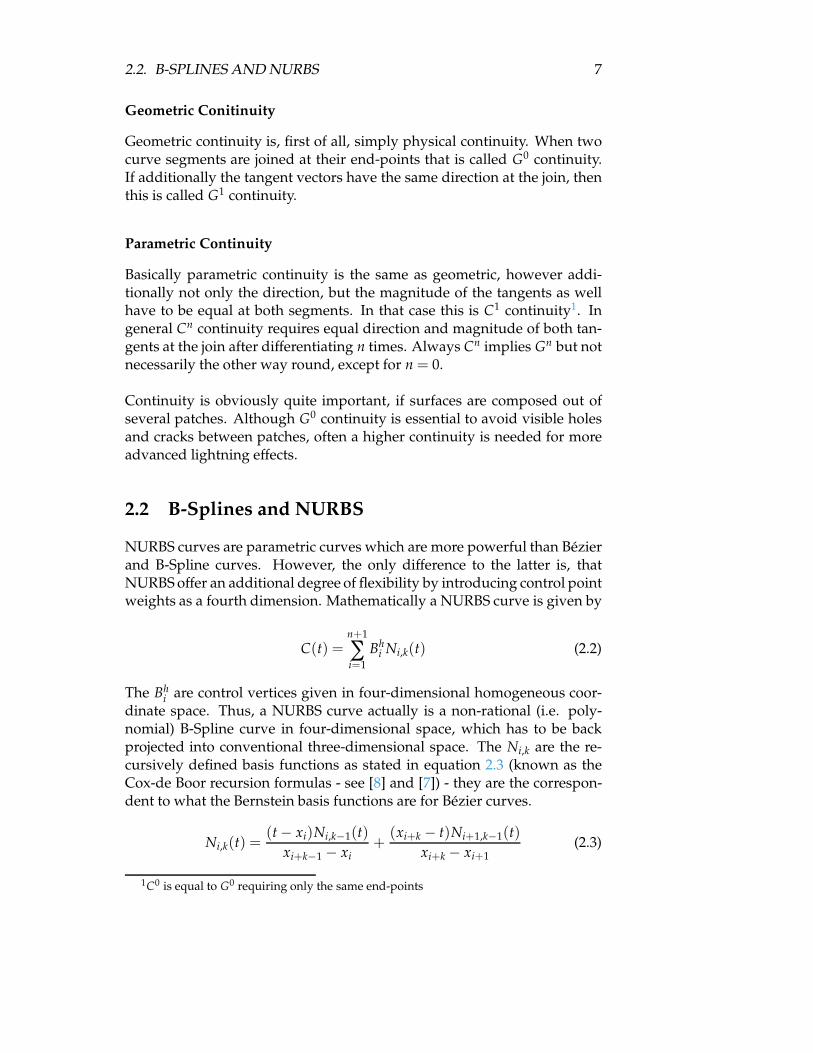
NURBS curves are parametric curves which are more powerful than Bézierand B-Spline curves. However, the only difference to the latter is, thatNURBS offer an additional degree of flexibility by introducing control pointweights as a fourth dimension. Mathematically a NURBS curve is given by
C(t) =n+1
∑i=1
Bhi Ni,k(t) (2.2)
The Bhi are control vertices given in four-dimensional homogeneous coor-
dinate space. Thus, a NURBS curve actually is a non-rational (i.e. poly-nomial) B-Spline curve in four-dimensional space, which has to be backprojected into conventional three-dimensional space. The Ni,k are the re-cursively defined basis functions as stated in equation 2.3 (known as theCox-de Boor recursion formulas - see [8] and [7]) - they are the correspon-dent to what the Bernstein basis functions are for Bézier curves.
Ni,k(t) =(t # xi)Ni,k#1(t)
xi+k#1 # xi+
(xi+k # t)Ni+1,k#1(t)xi+k # xi+1
(2.3)
1C0 is equal to G0 requiring only the same end-points

8 CHAPTER 2. BASICS
0
1
2
3
4
5
6
7
0 0.5 1 1.5 2 2.5 3 3.5 4
line 1line 2line 3line 4
Figure 2.2: The same NURBS curve with different weighting factor at B3(2/5). From top to bottom the weights are: 1000, 1, 0.1, 0
The recursion will stop when k equals 1. In this case equation 2.4 applies.
Ni,1(t) =
'
1 if xi " t < xi+10 otherwise
(2.4)
This recursive definition requires the convention 00 = 0 to be applied. It
is mandatory to avoid division by zero. Figure 2.2 shows four exemplaryNURBS curves, which have the same control points and identical knot vec-tors but differ in the weighting factor of a single control point.
2.2.1 Knot Vectors
The xi found in equation 2.3 are elements of a knot vector. The choice of theknot vector has a direct influence on the basis functions and therefore onthe curve itself. The number of elements of a knot vector is determined bythe sum of the number of control points and the order of the basis function.Furthermore the knot vector values have to be monotonically increasing, i.exi " xi + 1. There are two different kinds of knot vectors periodic and open,where both of them can either be uniform or non-uniform. A uniform knotvector has equidistant values usually beginning at zero like the followingexample shows
[0 1 2 3 4 5 6]
Often knot vectors are normalized
[0 0.33 0.66 1]

2.2. B-SPLINES AND NURBS 9
Curves with open or periodic knot vectors define slightly different curveshapes, however the biggest difference is to be found in the start- and end-points. The beginning of a curve with an open knot vector lies always ex-actly on the very first control point, respectively the end is found on thelast. Periodic knot vector curves unfortunately do not start and end at aspecific control point, so they are more complicated to handle for model-ing purposes. Periodic knot vectors are not considered any further in thiswork, nevertheless there is not an architectural issue that would preventan easy and straightforward integration of these in the library/applicationpresented here.
Open knot vectors always have a multiplicity of knot values at both theirends, equalling the order k of the basis function (k =degree+1). The in-ternal knot values are either evenly spaced or not depending wether thevector is uniform or non-uniform. The first example shows an open uniformknot vector for k = 3 and the second shows an open non-uniform knot vec-tor for k = 4
[0 0 0 1 2 3 4 4 4]
[0 0 0 0 0.5 1.2 3.8 4 4 4 4]
2.2.2 Basis Function Dependancy
A basis function of some given order k depends on lower basis functionsof order k # 1, with the exception for order 1 which is either 0 or 1. Notethat the Cox-de Boor formula is defined recursively (see equation 2.3). Thedependancies reveal a triangular pattern as follows
Ni,kNi,k#1 Ni+1,k#1Ni,k#2 Ni+1,k#2 Ni+2,k#2...Ni,1 Ni+1,1 Ni+2,1 Ni+3,1 · · · Ni+k#1,1
(2.5)
It is obvious, that even for low order NURBS curves the basis functions canbecome quite expensive to compute. The efficient evaluation of all involvedbasis functions is one of the most important challenges, since this is anessential task which has to be performed several million times in a secondin order to achieve interactive frame rates. In addition, the basis functionevaluation must be as exact as possible, unfortunately strictly excludingapproximative approaches, since the Newton iteration (5.2.2), used for theintersection test, is itself a numeric method. It is not advisable to feed itwith imprecise data since errors would accumulate fast.

10 CHAPTER 2. BASICS
2.2.3 Weighting Factors
Basically the only difference between NURBS and non-uniform B-Splinesis the extended flexibility of the former by introducing weighting factors.Usually control points with weighting factors are represented as homo-geneous coordinates in four dimensional space. If all weights of a givenNURBS surface equals 1, then the surface is just the same as a non-uniformB-Spline surface with identical control vertices. However, increasing aweight at any control point bends the surface towards that point as longas the weight is greater than one. Respectively negative weighting fac-tors will push the surface away from the control point. A value betweenzero and one indicates a weaker influence of the appropriate control point,while still not pushing the surface away. Finally, assigning zero as a weightcauses this control point to have no influence on the curve at all.
In order to have a curve defined in common 3D space the curve has tobe back projected from homogenous coordinates into common spacial di-mensions. Equation 2.2 yields
C(t) =∑n+1
i=1 BihiNi,k(t)
∑n+1i=1 hi Ni,k(t)
(2.6)
As mentioned before, negative weighting values can also be used as well,although they barely appear in real life circumstances, since they are quiteunpredictable in their behavior and additionally introduce some more orless serious problems. In nearly any case it is more feasible to describea surface by a more complex one, that uses positive weighting values (oreven none at all). The problems mentioned are as follows:
• The convex hull property may be destroyed
• Singularities may occur
• The surface shape will become quite unpredictable
The convex hull property can be important for the generation of boundingboxes (see section 3.2.2), depending on the employed technique. Althoughtheir usage is really not suggested they are fully supported by the workpresented here.
2.2.4 NURBS Properties
Since NURBS are a generalization of non-uniform B-Splines, they largelyhave the same characteristics. The most important are shortly outlined here
• All basis functions are zero or positive for all valid parameter values

2.2. B-SPLINES AND NURBS 11
• For any parameter value the sum of all basis functions is preciselyone for that value
• The maximum order equals the number of control points in that para-metric direction
• For all weights h > 0 the curve or surface lies in the convex hull whichis formed by the union of k successive control point vertices (see nextsection 2.2.5)
2.2.5 Convex Hull of B-Splines and NURBS
The convex hull property can be exploited for determining exact bound-ing volumes which are, of course, very important for any ray tracer (alsosee 2.6). However, convex hull determination is a bit more sophisticatedcompared to the same process for Bézier surfaces, where these can be cre-ated simply by taking the minimum and maximum coordinate values ofall control points of a single surface. This could be applied to B-Splines aswell, although this potentially will yield wrong results on some special oc-casions. Both approaches are investigated later in section 3.2.2.
The convex hulls for B-Splines are dependent on the degree of the basisfunction of a specific curve or surface. The higher the degree, the largerthe hulls will become. Figure 2.3 illustrates the effect of the basis functionorder on the convex hull. The two most extreme cases are
• k = 2: If the basis functions are linear segments, the convex hull iscompletely identical to the control polygon.
• k = #ControlPoints: If the basis functions have maximal degree (i.e.order is equal to the number of control points) the convex hull is justthe same as it would be in case of a Bézier curve/surface.
Note, that the curve or surface is usually not bounded by a single convexhull, which would only happen in the latter case. The number of convexhulls is equal to the intervals defined by the knot vector. For example aB-Spline curve with open knot vector [0 0 0 1 2 3 4 4 4] would be boundby four different convex hulls.
The convex hull properties for NURBS are nearly identical to the B-Splinesproperties. Positive weighting factors will never conflict with the proper-ties described above. Negative values instead may indeed do so, since sin-gularities can occur, which naturally will break any convex hull. In section3.2.2 an improved approach for bounding box generation will be presented,which is not dependent on the convex hull properties, thus offers a robustbounding volume generation for all kinds of surfaces.

12 CHAPTER 2. BASICS
Figure 2.3: The convex hull of a NURBS curve which is defined by fivecontrol points. Varying order of the basis functions shows the effect onthe size and number of convex hulls. The smaller the order the closer theconvex hull bounds the actual curve
2.2.6 Curve Refinement
As described in the previous section, bounding boxes can be created by us-ing a the convex hulls. However, depending on the surface, more boundingboxes than that are needed most of the time (the reason is explained in sec-tion 5.2). By subdividing a curve/surface it is possible to generate moreconvex hulls which in turn creates more boxes.
Refinement of NURBS requires to add more control points which increasesthe number of knot vector intervals. The surfaces’ shape remains identical,of course, by offering a higher degree of flexibility. Basically there are twocommon different ways to refine a NURBS curve.
First, the flexibility of NURBS can be increased by raising the degree ofthe basis functions, called degree elevation. This, however, will producelarger convex hulls and even reduces their number, which is contra pro-ductive in this context! In addition to that, the order of the curve can notexceed the number of control points, thus their number might have to beincreased as well which again raises complexity further, resulting in longercomputation time for any operation on the curve/surface.
The second approach is called knot refinement. The idea is, to simplysplit a polynomial segment into two piecewise new polynomial segments

2.2. B-SPLINES AND NURBS 13
for that given interval. This will create more parametric intervals, which inturn can be used to create more bounding boxes. However, in many cases itwill be necessary to initially refine over the whole curve/surface not onlya specific parametric interval, thus multiple knots have to be inserted atonce. Here the Oslo algorithm (see [10] for more detail) is shortly outlined,as this algorithm is capable to insert multiple knot values in a single step,which is to favor over the method developed by Boehm et al. [40], whichcan only insert one knot value at a time. Recall equation 2.2 now with thefollowing assigned knot vector
[x1 x2 . . . xn+k+1]
Generally by inserting an arbitrary number of new knot values the newknot vector will become
[y1 y2 . . . ym+k+1]
where m has to be greater than n. Thus the new curve can be described as
D(t$) =m+1
∑j=1
Chj Nj,k(t$)
As stated above the shape of the curve should be exactly the same after-wards, so the Ch
j need to be computed such that C(t) = D(t$). The new Chj
are given by
Chj =
n+1
∑i=1
"ki, jB
hj
with 1 " i " m as shown in [33]. The "ki, j are given recursively, similar to
the basis function recursion
"1i, j =
'
1 xi " yj " xi+10 otherwise
"ki, j =
yi+k#1 # xi
xi+k#1 # xi"
k#1i, j +
xi+k # yj+k#1
xi+k # xi+1"
k#1i+1, j
Here, too ∑n+1i "k
i, j = 1 does hold.
If uniform knot vectors should be preserved as such, some special atten-

14 CHAPTER 2. BASICS
tion has to be payed: To maintain these, it is necessary to add one new knotvalue midway in each parametric interval. The knot values are usuallymultiplied by two beforehand when using integer values to avoid fractions.
For example the knot vector
[0 0 0 1 2 2 2]
is first multiplied by two (optional)
[0 0 0 2 4 4 4]
and then the new values are inserted
[0 0 0 1 2 3 4 4 4]
A curve subdivided this way has the same degree as before, but more con-trol vertices and a longer knot vector with more intervals. Recall, thatthe number of knot vectors intervals specifies the number of convex hullsbounding the curve. Effectively every subdivision step doubles the num-ber of intervals, thus unfortunately only offering a quadratically increasein the number of intervals, thus bounding boxes to be generated.
A surface can be subdivided respectively by subdividing all splines of oneparametric direction the same way as described above. First subdividingalong u parametric direction and afterwards along v parametric directionwill yield the same result, as when swapping the order in which it is sub-divided.
2.2.7 Derivatives
The derivative for non-rational B-Spline curves at a given point can be ob-tained by formally differentiating, thus equation 2.2 will yield
C$(t) =n+1
∑i=1
Bhi N$
i,k(t) (2.7)
Obviously only the basis functions need to be differentiated, which again,for B-Splines can be done straight forward yielding
N$i,k(t) =
Ni,k#1(t) + (t # xi)N$i,k#1(t)
xi+k#1 # xi+
(xi+k # t)N$i+1,k#1(t) # Ni+1,k#1(t)
xi+k # xi+1(2.8)
However, by having a closer look at equation 2.4, it becomes apparent thatnow N$
i,1(t) = 0 for all t. The recursion is now terminated for k = 2, so that
N$i,2 =
Ni,1(t)
xi+1 # xi#
Ni+1,1(t)xi+2 # xi+1
(2.9)

2.2. B-SPLINES AND NURBS 15
With the new recursion formulas above, the values for the derivatives atany given point can be calculated. Also tangents, of course, can now becomputed, which are needed for the previously mentioned Newton itera-tion as well. The second derivative could be computed respectively, but asit is not needed in this context, it is not discussed here.
For NURBS curves the idea is basically the same, albeit it is a bit moresophisticated, due to the fraction that occurs with rational B-Splines. Byrewriting equation 2.6 into the shortcut notation n
d with n denoting thenominator and d the denominator, the first derivative can be expressed as
C$(t) =n$d # nd$
d2
where n$ was already derived above (see equation 2.7) and d$ can be com-puted just the same way.
2.2.8 NURBS Surfaces
NURBS surfaces are, obviously, the logical extension of their curve counter-part. Represented as a cartesian product, the following equation describesa NURBS surface (compare equations 2.2 and 2.6)
S(u, v) =∑n+1
i=1 ∑m+1j=1 Bi, jhi, jNi,k(u)Mj,l(v)
∑n+1i=1 ∑
m+1j=1 hi, jNi,k(u)Mj,l(v)
(2.10)
Here again, the Bi, j are the three dimensional control vertices, hi, j are thecorresponding weight values, Ni,k are the basis functions in the u paramet-ric direction and Mj,l likewise for the v direction. The properties of NURBSsurfaces are analogue to the properties for NURBS curves, so they need notto be repeated here.
NURBS cover both Bézier and B-Splines where the latter are simply NURBSwith all weighting factors equaling one. Bézier curves and surfaces are in-deed a special case of NURBS, when the basis functions actually reduce tothe Bernstein polynomials, which is the case, whenever the order of the ba-sis functions equals the number of control points and an open knot vectoris employed, for instance
[0 0 . . . 0 1 1 . . . 1]
The multiplicity of zeros and ones is corresponding to to the order of thebasis. In contrast to Bézier surfaces, NURBS are much more flexible andpowerful, thus allowing a more complex geometry description with lesssurfaces, which in turn means lesser memory consumption.

16 CHAPTER 2. BASICS
Subdivision or bounding box creation for surfaces is quite similar to thesame process for curves, only that the computations have to be done fortwo parametric directions for a single surface. For example a NURBS sur-face with a 5x5 control point net defines actually five NURBS splines inboth u and v parametric direction. Subdividing such a surface requires tosubdivide every of the five splines in one parametric direction and thensubdividing the resulting surface again in the other parametric direction.Each spline is subdivided accordant section 2.2.6, only that is has to bedone ten times for such a surface.
2.2.9 NURBS Surface Derivatives
Although NURBS derivatives are computed in a similar way as their non-rational counterparts, the process is a bit more complex, thus it might beworthwhile to discuss it in more detail. When computing the derivative ofa surface which is defined in two parametrical directions the partial deriva-tives are required. The partial derivative of a NURBS surface in u paramet-rical direction can be expressed as
Su =n
d
!
nu
n#
du
d
"
where again d denotes the denominator and n the nominator of equation2.10. Respectively
Sv =n
d
!
nv
n#
dv
d
"
where
nu =n+1
∑i=1
m+1
∑j=1
Bi, jhi, jN$i,k(u)Mj,l(v)
and
du =n+1
∑i=1
m+1
∑j=1
hi, jN$i,k(u)Mj,l(v)
Respectively
nv =n+1
∑i=1
m+1
∑j=1
Bi, jhi, jNi,k(u)M$j,l(v)
and
dv =n+1
∑i=1
m+1
∑j=1
hi, jNi,k(u)M$j,l(v)
Here the derivatives of the basis functions N$ and M$ are identical, of course,to the derivatives as they were introduced for single curves in section 2.8.

2.3. SHADING LANGUAGES 17
Algorithm 1: Cg example code
void main( float2 inCoord : TEXCOORD0,out float4 outColor : COLOR,uniform samplerRECT : texture)
{outColor = texRECT(texture, inCoord);outColor.a = 0.5;
}
2.3 Shading Languages
Since this work targets to present a cross-platform solution, one of the wellknown shading languages can not be considered, which is Microsoft’s Di-rectX [9], because it naturally runs on x86 Windows machines only. Thisbasically leaves a choice between Nvidia’s Cg (2.3.1) and the OpenGL Shad-ing Language (2.3.2), which both are available for Mac OS X, Linux as wellas Windows.
2.3.1 Cg
Cg (C for graphics) [24] was 2003 introduced by NVidia as a complete de-veloping platform for GPU programming. In principle all programmablegraphic boards are supported (for example GeForce FX and ATI Radeon9700 generation and above), but for ATI cards support is limited to ARBmultivendor specifications. This means for more advanced vertex pro-grams or fragment shaders a current NVidia card is required. For example,floating point textures are not available within the ARB specification.
Cg offers a C like syntax so it is very convenient to start with. The codesnipped 1 shows a basic fragment program that assigns a color value sam-pled from a texture and assigns a 50% transparency.
By using a high level language like Cg it is no longer necessary, even notworthwhile in most cases, to write assembler code. Another general posi-tive aspect of NVidia’s Cg is, that it can compile code for both major graphicAPIs OpenGL as well as DirectX.
2.3.2 OpenGL Shading Language
With the release of OpenGL specification 1.5, support for programmablevertex and fragment shaders was added by introducing the OpenGL Shad-

18 CHAPTER 2. BASICS
Algorithm 2: OGSL example code
const uniform sampler2DRect texture;
void main(){
gl_FragColor = texRECT(texture, gl_TexCoord[0]);gl_FragColor.a = 0.5;
}
ing Language [30] (GLSL). Since OpenGL is installed already on nearly ev-ery modern system, usually nothing particular has to be done in order todevelop vertex and fragment shaders. Cg, however, requires the Cg ToolkitSDK which has to be downloaded and installed. Shaders written in Cgneed to link against this library. Similar to Cg, OGSL has a C like syn-tax. The GLSL example 2 will have the same effect than the Cg example.Comparing the example code 2 with 1, the most striking difference is themissing parameter list in the latter. Textures and the like are referenced asglobal variables so they do not need to be passed to every function withinthe program. Other values like texture coordinates and output colors arereferenced as OpenGL global build-in variables which is quite comfortable.However, the real advantages of OGSL are to be found in excellent supportfor both NVidia and ATI cards, so by choosing OGSL as the language ofchoice, there is a broader range of graphic cards that will support the fullfeature set. Additionally OGSL offers SIMD commands similar to the onesthat will be used in the code for the CPU. Of course Cg supports SIMD op-eration as well, but it lacks some important features. For example the bool4data type is missing in Cg, however OGSL offers not only that, but a fullset of vector relational functions as well, like
bvec4 lessThan(vec4 a, vec4 b)
or
bvec4 any(bvec4 a)
This makes it easier to port the CPU code to the GPU as the commandsnearly map one-to-one. The intersection code was partially developed inboth shading languages. There was no real difference in performance, how-ever the code with OGSL is much cleaner, more maintainable and also eas-ier to synchronize with the code implemented for the CPU.

2.4. SIMD INSTRUCTION SET 19
2.4 SIMD Instruction Set
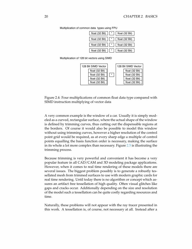
SIMD is an extension offered by most of the current CPU models and ar-chitectures. Intel’s implementation found on Pentium II processors andabove is called SSE and SSE2 on Pentium IV class processors respectively2.Motorola’s G4 as well as IBM’s G5 processors feature AltiVec (i.e. namedVelocityEngine by Apple) which is also a SIMD implementation. Basicallyboth different instruction sets offer roughly the same features, but one maylack some specific instruction of the other and vice versa. For example Al-tiVec offers an instruction that will multiply a and b and adds c to the resultwhich is perfectly suited for dot products, but SSE lacks such a commandand has to combine the common multiply and add commands. However,there is no simple multiply with AltiVec, which means a multiplication hasalways to be implemented as a MultiplyAdd where c equals zero. Both havein common that they do not work on common data types like int or float,but on vector data with a fixed witdh of 128 bits. Dependent on the pro-cessor the multiplication of two float values may take a specific numberof cycles. Apparently four multiplications will take four times as long (atleast when only one FPU is available). By using SIMD instructions thesefour multiplications can be carried out in parallel by storing four valueseach in a SIMD vector (4 % 32 bit = 128 bit), then one multiplication com-mand performs the operation on the whole 128 bit data vector, effectivelyyielding four results in parallel (see 2.4). However, the expected speed upof four can not be reached in real life circumstances because not every com-putation can be carried out in parallel and additionally often a small (ornot so small) overhead computation is required. For example, writing val-ues into a SIMD register is expensive, because data need to be aligned inmemory along 16 byte boundaries.
2.5 Trimming
All parametric surfaces tend to have a rectangular-like shape, which is dueto the rectangular parametric domain. By carefully choosing a certain knotvector, it is possible to overlay multiple control vertices at the same locationin space, which can reduce the above mentioned effect slightly. However,it is much more efficient and easier to model non rectangular like shapesby using so called trimmed surfaces. Certain regions in the parametric do-main are simply defined as invalid, thus all surface points defined by theseinvalid parametric values are considered not to be part of the surface, ef-fectively cutting the regions out.
2SSE3 can now be found on some of the most current processors from Intel
20 CHAPTER 2. BASICS
Figure 2.4: Four multiplications of common float data type compared withSIMD instruction multiplying of vector data
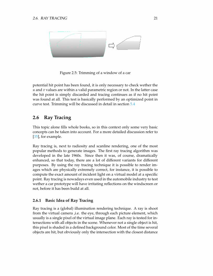
A very common example is the window of a car. Usually it is simply mod-eled as a curved, rectangular surface, where the actual shape of the windowis defined by trimming curves, thus cutting out the dispensable regions atthe borders. Of course it would also be possible to model this windowwithout using trimming curves, however a higher resolution of the controlpoint grid would be required, as at every sharp edge a multiple of controlpoints equalling the basis function order is necessary, making the surfacein its whole a lot more complex than necessary. Figure 2.5 is illustrating thetrimming process.
Because trimming is very powerful and convenient it has become a verypopular feature in all CAD/CAM and 3D modeling package applications.However, when it comes to real time rendering of these models there areseveral issues. The biggest problem possibly is to generate a robustly tes-sellated mesh from trimmed surfaces to use with modern graphic cards forreal time rendering. Until today there is no algorithm or concept which as-sures an artifact free tessellation of high quality. Often visual glitches likegaps and cracks occur. Additionally depending on the size and resolutionof the model such a tessellation can be quite costly regarding resources andtime.
Naturally, these problems will not appear with the ray tracer presented inthis work. A tessellation is, of course, not necessary at all. Instead after a
2.6. RAY TRACING 21
Figure 2.5: Trimming of a window of a car
potential hit point has been found, it is only necessary to check wether theu and v values are within a valid parametric region or not. In the latter casethe hit point is simply discarded and tracing continues as if no hit pointwas found at all. This test is basically performed by an optimized point incurve test. Trimming will be discussed in detail in section 5.4
2.6 Ray Tracing
This topic alone fills whole books, so in this context only some very basicconcepts can be taken into account. For a more detailed discussion refer to[35], for example.
Ray tracing is, next to radiosity and scanline rendering, one of the mostpopular methods to generate images. The first ray tracing algorithm wasdeveloped in the late 1960s. Since then it was, of course, dramaticallyenhanced, so that today, there are a lot of different variants for differentpurposes. By using the ray tracing technique it is possible to render im-ages which are physically extremely correct, for instance, it is possible tocompute the exact amount of incident light on a virtual model at a specificpoint. Ray tracing is nowadays even used in the automobile industry to testwether a car prototype will have irritating reflections on the windscreen ornot, before it has been build at all.
2.6.1 Basic Idea of Ray Tracing
Ray tracing is a (global) illumination rendering technique. A ray is shootfrom the virtual camera ,i.e. the eye, through each picture element, whichusually is a single pixel of the virtual image plane. Each ray is tested for in-tersections with all objects in the scene. Whenever not a single object is hit,this pixel is shaded in a defined background color. Most of the time severalobjects are hit, but obviously only the intersection with the closest distance

22 CHAPTER 2. BASICS
Figure 2.6: Basic principle of the ray tracing algorithm
to the camera is valid (unless that one is transparent). The incoming lightat that location will be computed afterwards, finally yielding a color valuebased on the material properties and the light that effectively is transmit-ted from all light sources in the scene to that point. The range of differentmethods that can be applied for these individual computation steps areranging from very simple and fast to highly complex. On the on hand, of-ten simple Phong shading [4] is used for computing the color value whichis not physically correct at all. On the other hand, sophisticated algorithmswhich, for example, take the BSSRDF [20] (Bidirectional Scattering SurfaceReflectance Distribution Function) of the surface into account, can be usedas well. Whatever method is used for shading, the ray tracing frameworklying underneath does not need to be changed.
Ray tracing systems generally are able to handle shadows, multiple reflec-tions, refractions and texture mapping with ease in a very straight forwardmanner. Additionally global illumination can also relatively easy be im-plemented by different variants of Monte Carlo ray tracing [32]. Figure 2.6shows the basic principle of ray tracing. The ray emerges from the camera(black box on the left side) and intersects two objects in the scene, the greencylinder and the red sphere. However, the intersection point with the greenobject is the closest to the camera, so the color green is assigned to that pic-ture element in the blue plane that is hit by the ray. This is simply done forevery picture element in the blue image plane. Extending this approach toalso incorporate effects like shadows and reflections for instance, is quiteeasy. If a surface, that has been hit, is reflective then a new ray has to be

2.6. RAY TRACING 23
cast from that point by calculating the reflected direction and recursivelycalling the trace routine with the newly computed ray. The result of thistrace is not used as a color value for the image plane, but scaled accordingto the reflectivity of the previously hit surface and added to its color. Trans-parency can be treated in just the same way by eventually computing tworays, one refracted and one reflected according to Snell’s law. Shadows areeven computationally easier. From a hit point a ray is casted towards thelight source. If any objects lies in between then no light from this source istransmitted to the intersection point. If that is the case for all light sourcesin the scene, this point will be shaded black (respectively in an ambientcolor).
2.6.2 Ray Tracing Acceleration Techniques
Ray tracing has the reputation of being very slow. However, by carefullyimplementing several acceleration techniques, ray tracing can become fastenough for an interactive setting nowadays. In turn this would mean,that without these, there would not be the slightest chance to become fastenough.
Bounding Volume Hierarchy
By reconsidering what was said in the last section, it becomes obvious thatthe computation time to render a single frame would increase linearly withthe number of objects (i.e. triangles, NURBS surfaces etc.) in the scene asevery single object has to be tested for an intersection with the ray. This canbe overcome by the usage of bounding volumes, where a single volume isrepresented by an easy geometry like a box or a sphere. This volume con-tains a number of objects and instead of the individual objects, the bound-ing volume itself is tested for an intersection. If the volume is missed, soare all contained objects. These volumes themselves can be organized inlarger volumes thus creating a bounding volume hierarchy. For example ifthe topmost volume, containing the whole scene, is missed, then the traceroutine for the current picture element will terminate after only one inter-section test with a box!
There are a lot of different approaches and techniques for more or less ef-ficient bounding volume hierarchies. A short overview as well as the ap-proach taken in this work can be found in section 3.2.

24 CHAPTER 2. BASICS
Parallelism
Ray Tracing is extremely well suited for parallel execution, since every pic-ture element that is being processed, is totally independent on all others.Basically it would be possible to have a single processor for every pictureelement. Unfortunately such machines are not available yet, but still it isvery attractive for multi core and/or multi processor systems. Even a clus-ter can be feasible, although network latencies can be a serious problemwhen targeting at interactive frame rates. The application dream, which isthe foundation of this work, has indeed been extended with network ren-dering capabilities. The scalability is still a subject to improvement, how-ever, first results justify further effort in that field. More details can befound in [3].
Fast Intersection Test
Obviously the intersection test itself is quite important, as it will be calledseveral million times for a single frame, depending on the frame size andscene itself. Regarding triangles, there are lots of different intersection algo-rithms, each with their own advantages and disadvantages in performance,memory consumption, preprocessing time and other factors. However, forNURBS surfaces the choices are rather limited, as this field was not so muchworked on, compared to the ray tracing of triangles. Any improvement inthe intersection test usually has a direct impact on overall performance ofthe whole system.
2.7 Basic Application Design Decisions
The software employs a range of different modules which might either beused or not, in order to be able to compare results with other approachesof ray tracing applications and also for the purpose of running it on olderhardware as well as uncommon architectures like the Itanium processorwhich does not feature a SIMD instruction set. The most important mod-ules are the intersection computation modules which there are three ofthem, namely a FPU (Floating Point Unit) emulation mode, SIMD andGPU. Figure 2.7 shows how these modules collude. The FPU emulationmode is a lot slower compared to SIMD powered execution. However, theFPU module is also a good candidate to compare results with completelydifferent ray tracers as most of them use the FPU only. Last but not leastby using the emulation mode, the application will run on every of the rackcomputer that has been sold in the last ten years as it’s only requirement isa floating point unit, though performance might be far from interactive inthat case, but still it would be possible to use the application as a fast, butnon-interactive, NURBS ray tracer anyway.

2.7. BASIC APPLICATION DESIGN DECISIONS 25
Figure 2.7: The upper blue part shows module choices for the CPU. Thelower yellow part for the GPU is optional. The dashed lines indicate, thatthe feature set is not yet comparable to the CPU implementation
If available, the SIMD unit takes advantage of either SSE or AltiVec de-pending on the processor type. Usage of SIMD instructions boosts the per-formance by more than 400%3 compared to the emulation mode and shouldbe used if SIMD extensions are available to the processor (beginning withPentium II or G4 class processors). Note that, of course, only either FPU orSIMD can be used at a time, not both!
Finally, usage of the GPU is optional and additional to the above men-tioned modules. However, as stated earlier at least a GeForce 6800 graphicsboard is needed, as older cards do not offer some of the needed functional-ity which is inevitable for the employed algorithm.
Figure 2.8 shows how the individual components work together. Basicallyany software that can handle NURBS data and supports the IGES file for-mat can be used to create scenes for crianusurt. Alias’s Maya for instanceis a software offering these features4. Both applications iges2dsd and cri-anusurt (chapter 5) rely on functionality offered by the libraries libNURBS(section 4.2) and libSIMD (section 4.1). Note that libSIMD uses only one of
3Theoretically the maximum speedup is factor 4, but the emulation mode is an emulationas the name says, so there is some additional overhead involved. An optimized FPU basedray tracer would be a bit faster than 25% of SIMD performance
4The IGES importer/exporter module has to be activated in the plugins preferencepanel. By default this plugin is deactivated

26 CHAPTER 2. BASICS
Figure 2.8: The system components and their relation to each other
the three modules (AltiVec, SSE, FPU) at once. In order to change the usedmodule, the library has to be recompiled. Both, libSIMD and libNURBSIn-tersectionKernel can be used by any other application as well.

Chapter 3
Preprocessing
The task of rendering NURBS surfaces need quite some preprocessing com-putation in order to get the intersection test as fast as possible. The follow-ing sections will give a overview about different ways on how the eval-uation of NURBS surfaces can be performed and motivates the approachtaken in this work. The application iges2dsd is responsible for the prepro-cessing. Iges2dsd is an application on its own and totally independent fromthe main rendering application. As input data it can take IGES files (seesection 3.1.1) or custom VRML-like files (section 3.1.2), as they are usedwith the Open Ray Tracing (OpenRT) [31] system of the realtime ray tracingworking group in Saarbrücken. After preprocessing is completed a custombinary dsd file is written. This file can be read later by the render applica-tion, thus the preprocessing step is, of course, necessary only once, unlessfor example the parameters for the bounding box volume generation arechanged.
After giving a general introduction to different bounding volume hierar-chies and space subdividing approaches in section 3.2, two variants whichwere implemented are discussed in more detail. Section 3.3 investigates thenecessart pre-processing for trimming curves, where section 3.4 is about theimprovement of the surface evaluation methods, which is very importantfor this work. Finall section 3.5 is about the memory layout for both, CPUand GPU, which differ from each other naturally.
3.1 File Loader
Currently the loader can read two different input files. However certainrestrictions apply, because NURBS surfaces are the only supported primi-tive1. VRML and especially IGES offer a lot of functionality which is not
1Bicubic Bézier surfaces are also supported as a special case which speed up the inter-section test significantly
27

28 CHAPTER 3. PREPROCESSING
needed in this context. Any unknown entity encountered during loadingwill simply be ignored, thus adding triangles to the scene, for example, willnot stop the loader from working, but it will not change the rendered scenein any way. The following sections give a quick overview of the capabili-ties.
3.1.1 IGES File Format
The IGES file format is a good candidate for data exchange from any mod-eling application like Maya [2] to crianusurt. It is possible to store NURBSsurfaces lossless, where most other file formats only store triangular ap-proximations of free form surfaces. IGES entity type 128 is reserved forstoring rational B-Spline surfaces. This is the only geometric entity parsedby the loader2, except for trimming curves. As mentioned above, everyother entity found will be ignored.
3.1.2 Customized VRML File Format
The above mentioned working group of Philipp Slusallek extended theVRML file format with a new tag to store bicubic Bézier surfaces. Thesefiles can be read by iges2dsd to test the optimized rendering of bicubic Béziersurfaces. However an explicit representation by NURBS can be enforced.Additionally the light sources and the camera stored in the file are also in-terpreted.
3.2 Bounding Box Volume Hierarchy Generation
Basically there are currently two different, concurrent classes of methodson how to reduce the number of objects which have to be tested for inter-sections. Bounding volume hierarchies are used since the very early daysof ray tracing, whereas different space partitioning methods are becomingmore popular in recent years.
3.2.1 Space Partitioning
Some of the better known variants that fit into this class are Oct-Trees [13],BSP-Trees [14] and kd-Trees [17].
Oct-Trees
Oct-trees are able to adapt to the scene. In the beginning the whole scene isregarded as one voxel. By employing a heuristic function which may take
2Bicubic Bézier surfaces, as a special case of B-Spline Surfaces, are also included in type128

3.2. BOUNDING BOX VOLUME HIERARCHY GENERATION 29
Figure 3.1: Exemplary Oct-Tree subdivision in 2D space. Regions withmore objects have a higher density of voxels. The ray has to test four voxelsand two objects, however a smart implementation would stop after the firstvoxel, because it is not possible to find a closer intersection
the number of objects and the depth of the tree into account, the voxel canbe split up into eight new voxels of the same size each. This is repeated re-cursively until no further subdividing is necessary or possible. Regions inspace with many objects will have a higher resolution voxel grid, whereaslarge empty regions are bounded only by a few big voxels. However, it canoccur that still some objects lie within more than one voxel so that the trac-ing algorithm has to keep track of which objects have already been tested toavoid multiple intersection tests on those. Figure 3.1 shows an 2D exampleof an Oct-Tree (which actually reduces to a Quad-Tree in a 2D case)
BSP-Trees
BSP-Trees (binary space partitioning) divide the space into two equal sizedhalf spaces by using a plane which separates them. It is possible to usean arbitrary plane for that, but due to a much easier intersection test it isadvantageous to use a plane that is perpendicular to one of the coordi-nate axis. The resulting hierarchy will bound the scene objects a bit closerthan an Oct-Tree. However, even better result can be achieved when thedividing plane is not placed in the geometric middle, but in such a way,that a cost function will be minimized. This kind of tree is referred to ask-dimensional trees (k-d trees).
kd-Tree
K-d trees adapt to the structure of the scene extremely well. If two new halfspaces are created, then each one will contain the same number of objects3,thus the number of objects to test against is halved with every subdivisionstep. This is recursively repeated until a maximum depth has been reached
3+/-1 if number of objects in parent space was odd
30 CHAPTER 3. PREPROCESSING
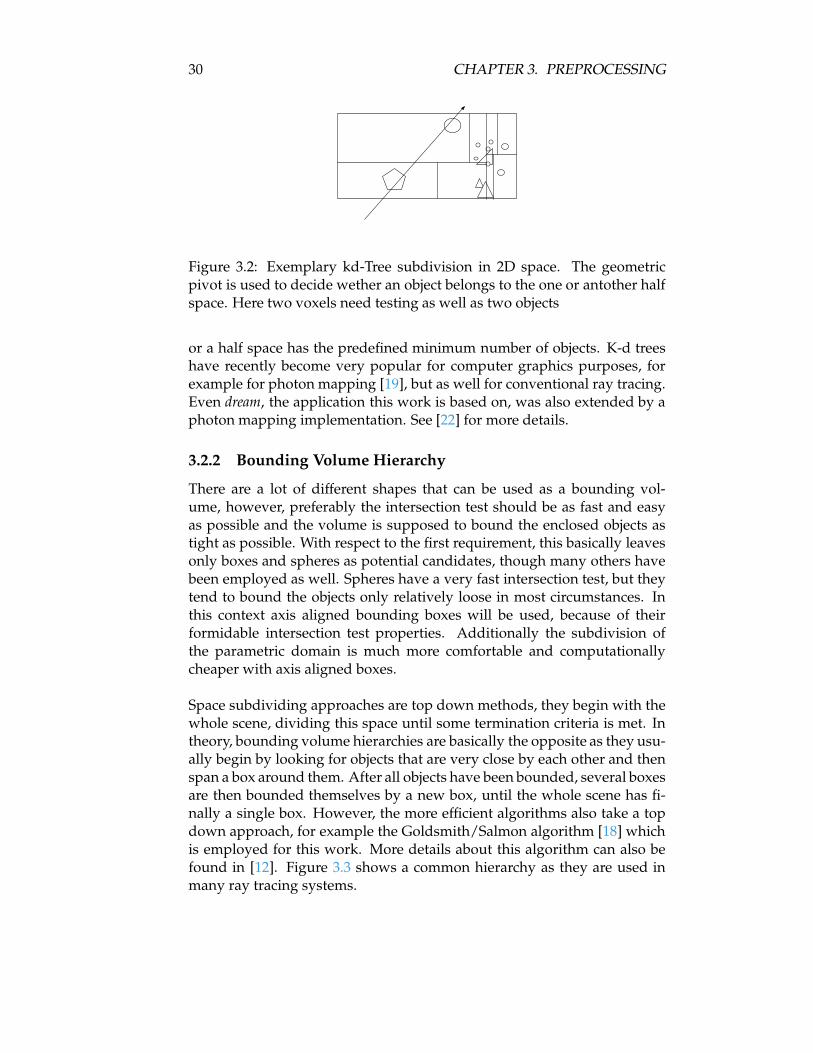
Figure 3.2: Exemplary kd-Tree subdivision in 2D space. The geometricpivot is used to decide wether an object belongs to the one or antother halfspace. Here two voxels need testing as well as two objects
or a half space has the predefined minimum number of objects. K-d treeshave recently become very popular for computer graphics purposes, forexample for photon mapping [19], but as well for conventional ray tracing.Even dream, the application this work is based on, was also extended by aphoton mapping implementation. See [22] for more details.
3.2.2 Bounding Volume Hierarchy
There are a lot of different shapes that can be used as a bounding vol-ume, however, preferably the intersection test should be as fast and easyas possible and the volume is supposed to bound the enclosed objects astight as possible. With respect to the first requirement, this basically leavesonly boxes and spheres as potential candidates, though many others havebeen employed as well. Spheres have a very fast intersection test, but theytend to bound the objects only relatively loose in most circumstances. Inthis context axis aligned bounding boxes will be used, because of theirformidable intersection test properties. Additionally the subdivision ofthe parametric domain is much more comfortable and computationallycheaper with axis aligned boxes.
Space subdividing approaches are top down methods, they begin with thewhole scene, dividing this space until some termination criteria is met. Intheory, bounding volume hierarchies are basically the opposite as they usu-ally begin by looking for objects that are very close by each other and thenspan a box around them. After all objects have been bounded, several boxesare then bounded themselves by a new box, until the whole scene has fi-nally a single box. However, the more efficient algorithms also take a topdown approach, for example the Goldsmith/Salmon algorithm [18] whichis employed for this work. More details about this algorithm can also befound in [12]. Figure 3.3 shows a common hierarchy as they are used inmany ray tracing systems.

3.2. BOUNDING BOX VOLUME HIERARCHY GENERATION 31
Figure 3.3: An example for a common bounding volume hierarchy. Theboxes represent bounding volumes, where each triangle represents a geo-metric primitve, which is a triangle itself in most cases
All children can be skipped, if the parent bounding volume was not hit.Although in many circumstances space subdividing methods, especiallykd-trees, are considered to be faster, bounding volumes were used for thiswork. One of the main reasons is, that bounding boxes can have a closerrelationship to the objects they are actually bounding. As explained laterin section 5.2.3 good initial guesses for starting the Newton iteration arerequired. These can be provided by the bounding volume hierarchy easily.Using a space partitioning scheme however, is not an adequate solution forobtaining such guesses, since there is no direct correlation to the surfaces,only to space itself. Good initial guesses are mandatory, thus boundingvolumes, which can provide these, are the only option in this context.
Bounding Volume Hierarchy for NURBS
Basically the hierarchy employed in this work is quite similar to the com-mon hierarchies used in other ray tracing systems, including dream, how-ever there is one very important difference. Usually a single bounding vol-ume has a few children which are either other bounding volumes or ge-ometric primitives. In this work however, a single NURBS surface needsto be bounded by a couple up to a few hundred bounding volumes, de-pending on the complexity of the surface (15 are an average value for low-complexity surfaces). Figure 3.4 shows two examples of scenes, where onlythe bounding boxes were rendered roughly4.
A high number of bounding boxes is necessary to achieve good initialguesses for the Newton iteration, but also to avoid unnecessary intersec-
4Actually always four neighboring pixels will always yield the same result, i.e. colorvalue, because a specific bounding box render mode was node implemented. Basicallythis is an interesting side effect, of an extremely large threshold parameter used during theNewton Iteration

32 CHAPTER 3. PREPROCESSING
Figure 3.4: The surface on the left side is bounded by 59 boxes whereas theface on the right has 13842. In the latter case the bounding boxes are sosmall that actually the shape of the object is visibly approximated by them.
Figure 3.5: An example for the bounding volume hierarchy employed inthis work. Every surface is bounded by several volumes.
tion tests with NURBS surfaces. A single test with a NURBS surface is farmore computationally expensive compared with a triangle intersection, soit is important to avoid as many unnecessary operations on NURBS as pos-sible, even if some additional bounding box tests are required in turn.
In the first place it seems that this will produce a huge amount of bound-ing volumes. However, the actual number of generated volumes will stillbe comparable or even less to common triangles scenes as a single NURBSsurface can describe geometry that otherwise would have been approxi-mated by possibly hundreds or thousands of triangles, requiring a largenumber of bounding boxes themselves.
3.2. BOUNDING BOX VOLUME HIERARCHY GENERATION 33
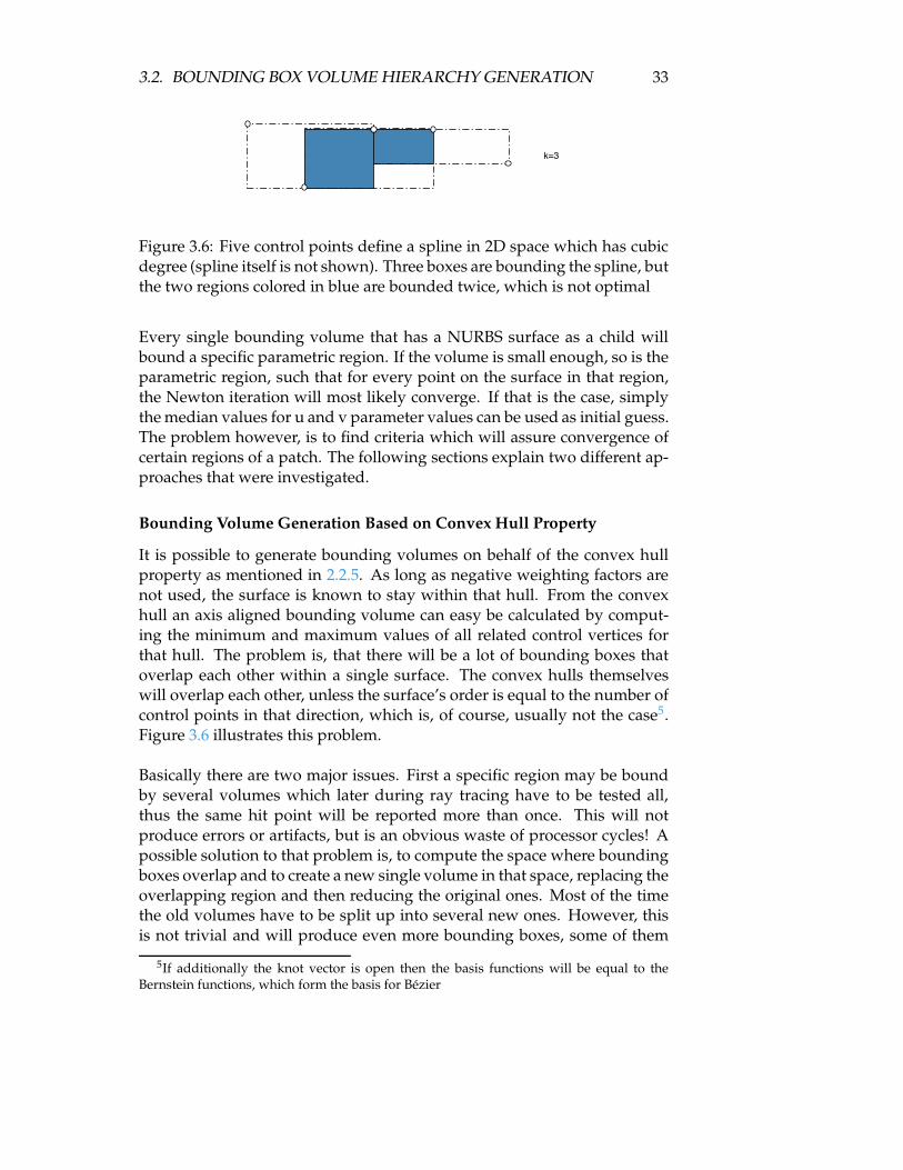
Figure 3.6: Five control points define a spline in 2D space which has cubicdegree (spline itself is not shown). Three boxes are bounding the spline, butthe two regions colored in blue are bounded twice, which is not optimal
Every single bounding volume that has a NURBS surface as a child willbound a specific parametric region. If the volume is small enough, so is theparametric region, such that for every point on the surface in that region,the Newton iteration will most likely converge. If that is the case, simplythe median values for u and v parameter values can be used as initial guess.The problem however, is to find criteria which will assure convergence ofcertain regions of a patch. The following sections explain two different ap-proaches that were investigated.
Bounding Volume Generation Based on Convex Hull Property
It is possible to generate bounding volumes on behalf of the convex hullproperty as mentioned in 2.2.5. As long as negative weighting factors arenot used, the surface is known to stay within that hull. From the convexhull an axis aligned bounding volume can easy be calculated by comput-ing the minimum and maximum values of all related control vertices forthat hull. The problem is, that there will be a lot of bounding boxes thatoverlap each other within a single surface. The convex hulls themselveswill overlap each other, unless the surface’s order is equal to the number ofcontrol points in that direction, which is, of course, usually not the case5.Figure 3.6 illustrates this problem.
Basically there are two major issues. First a specific region may be boundby several volumes which later during ray tracing have to be tested all,thus the same hit point will be reported more than once. This will notproduce errors or artifacts, but is an obvious waste of processor cycles! Apossible solution to that problem is, to compute the space where boundingboxes overlap and to create a new single volume in that space, replacing theoverlapping region and then reducing the original ones. Most of the timethe old volumes have to be split up into several new ones. However, thisis not trivial and will produce even more bounding boxes, some of them
5If additionally the knot vector is open then the basis functions will be equal to theBernstein functions, which form the basis for Bézier

34 CHAPTER 3. PREPROCESSING
which might even become useless, as the do not bound a part of the sur-face anymore. Although this can be done during preprocessing, it will stillrequire a great amount of computation power and leaves another problem:The correct computation of the newly bound parametric domain. Secondthere is the lack of flexibility of the generation process. The surface canbe refined by adding new values to the knot vector, which in turn will in-crease the number of knot vector intervals, i.e. the number of convex hulls.However this process is quite expensive (with respect to runtime) and itcan not be controlled very well. Each time the number of convex hulls willincrease super linearly. Other refinement methods, like control point inser-tion, suffer from similar problems. Subdivision was discussed in section2.2.6. Whenever any kind of subdivision is performed, the original surfacehas to be kept, of course, because the refined surface is describing exactlythe same surface in a more complex way.
Considering all this, a different approach seems to be (and will prove tobe - see results section 7.5) much easier and a lot better in performance.
Bounding Volume Generation Based on Surface Flatness Criterion
The basic idea of this approach is, that a surface, which is very flat, is op-timal for convergence with an arbitrary starting guesse somewhere on thesurface and thus need not to be refined further. However a surface withstrong curvature is most likely a good candidate for further subdivision.Flat surfaces will have normals which are roughly equal in direction to eachother. By computing several normals at different positions on the surface itis possible to estimate a measure for the curvature of that surface (or sub-surface). In this work eight normals are taken into account as shown infigure 3.7, simply because a multiple of four can take the greatest advan-tage of the SIMD implementation, i.e. eight normals are roughly computedas fast as normally two would with a FPU implementation!
It is possible to construct special surfaces that would not be handled cor-rectly by this technique - for example when a surface would have an ex-tremely sharp peak in the middle of the surface. However, these surfacesoccur rarely in real life and tests of several different scenes have shown noproblems. If visible artifacts occur, which are caused by this approach, thenstill the convex hull based generation mode can be used.
The surface would be perfectly flat if
#7i=1ni % ni+1 = 1
does hold, where the ni are the normal vectors. However, whenever ni %ni+1 < 0 occurs, the process is interrupted and the result is reported as 0

3.2. BOUNDING BOX VOLUME HIERARCHY GENERATION 35
Figure 3.7: The blue circles mark the positions where normals will be eval-uated
Figure 3.8: The normal samples taken may satisfy the flatness criterion (de-pending on the chosen constant) but the peak in the middle of the splineis not recognized properly and the generated bounding box (dashed box)will not include it
immediately, as in this case the surface is bend so hard, that a subdivisionis necessary anyway. Considering this, the result of the product will alwaysbe between 0 and 1 with values close to 1 denoting a relatively flat surface.
If a surface is considered flat, then the coordinate values at the four edgesare used to determine the bounding volume. At this point the above men-tioned error might occur. Figure 3.8 shows an example in 2D where thistechnique may fail.
Any surfaces that do not satisfy the flatness criterion will be further recur-sively subdivided. In order to keep it simple and fast, the original surfacesparametric domain will be divided into four (parametric) equally sizedsub-surfaces. The one point shared by all four subpatches is therefore tobe found at S(0.5, 0.5), assuming normalized knot vectors. The processwill be repeated on them unless a maximum depth is reached or the sur-

36 CHAPTER 3. PREPROCESSING
face is considered flat enough. By using the parametric middle, the surfacewill not necessarily be divided into parts with equal face area (for surfaceswith non-uniform knot vectors to be exact), but the advantage is that thenew parametric domains for the sub-surfaces come for free.
With this approach it is now possible to seamlessly adjust the number andquality of bounding volumes generated.
• Choosing a constant f with f ! [0, 1] so that every surface flatnesscriterion result p with f < p " 1 denotes a surface that does not needfurther subdividing
• Choosing a maximum subdivision depth to limit the possible maxi-mum number of volumes
• Increasing the number of normals used for flatness estimation to im-prove accuracy further (for very complex surfaces)
These properties offer a configurability that will suite all scenes in a conve-nient and efficient way. For most scenes, values for f between 0.8 and 0.9will yield good results, increasing that value will create more and smallerbounding boxes. The maximum subdivision depth should not be morethan 8, although often 6 will also be sufficient. Using more than 8 normalsfor flatness estimation has brought no improvement so far, but could beuseful with unusual or extremely complex scenes.
3.3 Trimming Curves
Most CAD/CAM applications today are able to render an image of the cur-rent scene by using the ray tracing technique. However, of course, none ofthese do not target interactive frame rates. This also is a reason why of-ten the trimming curves are represented as ordinary B-Spline curves. Inorder to achieve interactive frame rates, it is useful or even mandatory toreduce the complexity of these curves. Otherwise most of the renderingtime would be spend computing the trimming test rather than the actualintersection point. In the previous work (see [1]) it was shown that usingcubic Bézier curve segements as trimming curves is very well suited re-garding accuracy and performance. The approach taken can be perfectlyported to the more complex NURBS surfaces, since it does not matter whatkind of parametric surface is employed, as long as it is using a two dimen-sional parametric domain.
Basically a trimming test has to be performed for any potential hit pointfound on a surface which has trimming curves assigned to it. However,

3.3. TRIMMING CURVES 37
Figure 3.9: The different cases of pre-classification from left to right: 1)area where no trimming test has to be performed 2) region that is cut outcompletely 3) region that needs trimming 4) complete surface rendered cor-rectly
often large surfaces have cut out only a small minor part and most of thetrimming tests will yield the very same result. In order to avoid as manyunnecessary tests as possible a pre-classification method is presented in thefollowing section.
3.3.1 Pre-Classification
As mentioned in the previous section (3.2.2), there are a number of smallbounding boxes for each individual surface. This is actually a great advan-tage for the trimming test, since a great number of the bounding boxes canbe pre-classified. During the preprocessing it is checked which of the threefollowing cases applies to each individual box
• Complete enclosed domain is untrimmed, thus trimming test canskipped during rendering
• Complete enclosed domain is trimmed, thus bounding box can bedeleted
• Domain is partially trimmed, thus trimming test has to be performedduring rendering
The first case means, that all bounding boxes with a completely untrimmeddomain are actually treated like rendering an untrimmed surface, becauseany hit point found, would obviously lie automatically within a valid para-metric range. The second case is especially interesting, as this reduces thecomplexity of the scene by removing whole bounding boxes, because ev-ery hit point found within that bounding box would be marked as invalidanyway. This only leaves the last case, where a pre-classification is not pos-sible, thus a trimming test has to be performed during runtime. Figure 3.9shows the three individual cases on the basis of a simple single surface.

38 CHAPTER 3. PREPROCESSING
Figure 3.10: A bounding box and a single trimming curve (part of a com-plete set of trimming curves) are shown here. The dots at the corners markthe locations where the classification test is performed. All of them willbe classified as not trimmed and thus disabling trimming test for this box,which in this particular case is wrong. Another test halfway between allcorners would correct that error, as the lower middle point would havebeen classified as trimmed then
To classify a bounding box, simply all four corner values of the parametricdomain are tested to check wether they are trimmed or not. Although pos-sibly errors can occur like shown in figure 3.10, these have not been seenin real life models so far, which might be due to the fact that cubic Béziersplines tend to be most trivial in terms of complexity6 (i.e. no sharp, un-predictable curves) and the bounding boxes are quite small as required forthe intersection test. Considering that, this approach is reasonable and fast.Additionally it would be possible to increase the accuracy of this techniqueby simply using more than four points for the classification process. Notethat a more detailed discussion on how the trimming test is actually beingperformed, can be found in section 5.4.
3.3.2 Trimming Curve Requirements
A trimming curve may be composited out of an arbitrary number of in-dividual curve segments. However, it is mandatory that this compositedcurve is closed. If there are holes in between neighboring segments, theapplication will still run, but it will yield wrong trimming results. Addi-tionally only cubic Bézier curves are supported, where any B-Spline curvewith cubic basis function degree will be converted automatically to a num-ber of piecewise cubic Bézier curves. Lines are currently represented byBézier curves as well, which of course, should be optimized in the future.
6Actually often a single trimming curve segment is so small that they are nearly linear

3.4. IMPROVING SURFACE POINTS EVALUATIONS 39
Algorithm 3: Naive approach to basis function evaluation
float basisFunction(int i, int k, float t, float* knot){if (k == 1){
if ((knot[i] <= t)&&(t < knot[i+1])) return 1;else return 0;
}
float z1 = (t - knot[i]) * basisFunction(i,k-1,t,knot);float n1 = knot[i+k-1] - knot[i];float z2 = (knot[i+k] - t) * basisFunction(i+1,k-1,t,knot);float n2 = knot[i+k] - knot[i+1];
float b1,b2 = 0;if (!(z1==0)&&(n1==0)) b1 = z1/n1;if (!(z2==0)&&(n2==0)) b2 = z2/n2;return simd_add(b1,b2);}
3.4 Improving Surface Points Evaluations
The evaluation of surface points (including their partial derivatives) is ofvery special importance, since it is an essential operation of the ray tracer.Depending on chosen parameter values for the intersection test and alsodepending on the individual surface the number of evaluations necessarymay vary. As shown later (see 5.2.3) in average around 11.5 evaluationsand partial derivative evaluations are needed per intersection test, so it isobvious that the evaluation method is a natural candidate for a maximumof optimization! The following sections will first show an easy brute forceapproach, which is rather slow, but will be improved incrementally, finallyyielding a fast polynomial representation of NURBS surfaces.
3.4.1 Naive Brute Force Approach
The most straight forward approach would be a brute force evaluation ofthe basis functions. The code snippet 3 shows an exemplary implementa-tion. Although this is very easy and fast to implement, it is totally unsuit-able for an interactive environment as the results in section 7.2 attest.
There are several serious performance issues with such an implementation.First, by looking at the basis function dependancies (see 2.5), it is obvious,that for each surface evaluation quite a number of basis functions are com-

40 CHAPTER 3. PREPROCESSING
puted several times each, especially when using high order surfaces withmany control vertices. The waste in computation power increases linearlywith the number of control points but quadratically with the degree of thebasis function. Additionally a recursive function call cannot be inlined7 bythe compiler, which is an additional loss in performance when a functionis called several million times per second. Finally the numerous if-then-else constructs can slow down computation speed further, since whenevera branch prediction fails the CPU has to be stalled while the pipeline runsempty.
3.4.2 SIMD Improved Approach
Some of the issues mentioned in the last section can be addressed by usingSIMD instructions which will compute four values in parallel, but addition-ally eliminate the need for some dynamic branching. Algorithm 4 showsanother exemplary implementation. Although this is an improvement byaround factor four it still can not address the problem of exponential in-creasing computation time of more complex surfaces. A solution is pre-sented in the next section.
3.4.3 Avoiding Recursion
In order to improve performance by more than an order of magnitude, itis obviously necessary to avoid the multiple computation of the same ba-sis function values over and over again, which basically means avoidingthe recursion at all in some way. On the one hand, a recursive functionnormally looks more like the original formula and is easy to implement,but more computation effort is needed. On the other hand, an iteration issometimes difficult to derive from an recursion, but most of the time it per-forms significantly better. In general it is always possible to turn any recur-sion into an iteration. However, this often requires a stack data structure,which is not optimal for use with SIMD instructions and not even possibleto implement on today’s GPUs without expensive tricks and workarounds.Since this work targets to use both the CPU and GPU in the best way possi-ble it is more reasonable to look for a way that is useful to both processingunits.
By having a closer look at the resulting basis function formulas it becomesevident, that these are in fact common (non rational) polynomials with amaximum degree corresponding to the given NURBS basis function de-
7For inlined functions the function call we be replaced by a copy of the code. This avoidsexpensive functions calls but also increases the size of the binary. Recursive functions cannot be inline as this would result in an endless loop.

3.4. IMPROVING SURFACE POINTS EVALUATIONS 41
Algorithm 4: Improved evaluation by using SIMD instructions
float4 basisFunction(int i, int k, float4 t, float4* knot){//check if recursion has to stopif (k == 1){
bool4 sel = simd_and(simd_cmple(knot[i],t),simd_cmplt(t,knot[i+1]));
return simd_select(mOne, mZero, sel);}
//simple Cox-de Boor recursionfloat4 z1 = simd_mul((simd_sub(t,knot[i])),
basisFunction(i,k-1,t,knot));float4 n1 = simd_sub(knot[i+k-1], knot[i]);float4 z2 = simd_mul((simd_sub(knot[i+k], t)),
basisFunction(i+1,k-1,t,knot));float4 n2 = simd_sub(knot[i+k], knot[i+1]);
float4 b1,b2;
//every zeroMask component is true for every n1 comp. = 0bool4 zeroMask = simd_cmpeq(n1,mZero);//SIMD zero division does not cause application to crashb1 = simd_div(z1,n1);//every comp. in b1 with corresponding zero comp. in zeroMask//will be replaced by zero, since convention 0/0=0 is appliedb1 = simd_select(b1,mZero,zeroMask);
//analog to the previouszeroMask = simd_cmpeq(n2,mZero);b2 = simd_div(z2,n2);b2 = simd_select(b2,mZero,zeroMask);
return simd_add(b1,b2);}

42 CHAPTER 3. PREPROCESSING
gree, but often these even reduce to simply zero8! In case of rational sur-faces the basic functions can be expressed as a fracture of non rational poly-nomials. However, due to the recursive nature of the basis function defini-tion the computation of these polynomials is not very straightforward andrequires some preprocessing. Fortunately the resulting polynomials canbe stored and used for the next run of the application without needing torecompute these, as long as the NURBS properties do not change. Modifi-cations in the control point coordinates are possible, however, changes inthe knot vector or basis function degree would require a re-computation ofall basis functions.
The benefits are obvious: not only is the recursion avoided but addition-ally the required computation effort is reduced remarkably, because onlythe simple and fast evaluation of polynomials is necessary. This can bedone very efficiently using Horner’s scheme [38] on the CPU or by bruteforce on the GPU, since the pow() command maps to a native instruction onthe GPU.
3.4.4 Basis Function Precomputation
The number of basis functions that need to be computed is dependenton the NURBS surface. Unfortunately the basis functions are also depen-dent on the parameter intervals of their corresponding knot vectors whichmeans that a number of basis function polynomials equalling the functionorder is needed for every interval defined by the knot vectors of each para-metric direction. The following equation shows how many functions areneeded for a specific NURBS surface
c = (#itKnotsU + 1) % #(degreeU + 1) + (#itKnotsV + 1) % #(degreeV + 1)(3.1)
Here #itKnots denote the number of internal knot values either in u para-metric direction or v, whereas #degree is denoting the degree of the basisfunctions in the according direction. For example, a NURBS Surface withfour control points in each direction and with both knot vectors having nointernal knot (thus degree 3), 8 basis functions would need to be computedand stored. The challenge is to do this computation efficiently and pre-cisely. An analytic approach might be more complex than some numericalapproximation, but as numerical errors can be avoided here, the analyticcomputation of the basis functions is definitively more reasonable, sincethere will be numerical errors made inevitable during the Newton’s iter-ation, that will be employed for the intersection tests. Also compare the
8A specific basis function is always completely zero for a given interval if the currentcontrol point has no influence on the surface in that region at all - this does happen espe-cially often for surfaces with a large number of control points and a low degree
3.4. IMPROVING SURFACE POINTS EVALUATIONS 43
results on issues with limited numerical accuracy shown in section 7.9.
The approach for analytic basis function pre-computation developed in thiswork is basically a two pass algorithm. As mentioned earlier, each basisfunction is dependent on two lower order functions, except for those withorder one, which are either one or zero, depending on the deployed param-eter value. First, a tree will be expanded by recursively expanding everybasis function according to equation 2.3, yielding a broad tree structurewith a depth equalling the NURBS basis function degree (see next section3.4.4 for more details). Second, for each parametric interval and for bothparametric directions a separate basis function will be computed by insert-ing one representative value of each interval into the tree, which will yielda simple polynomial after evaluating each element of the tree bottom upwise (see 3.4.4).
1st Pass: Tree Construction
By having a closer look at the basis function definition (equation 2.3) it be-comes obvious, that these are actually the sum of two very similar fractionseach of which has a real number as denominator and a product of a realnumber and a lower order basis function as numerator. The fraction can beturned into a product as well by taking the reciprocal value of the denom-inator leaving the sum of two three-component products. This scheme isthe same for all basis functions, except for order one functions, which haveto be handled separately later. Figure 3.11 shows the first two steps duringthe tree construction phase. The final depth of the tree corresponds to theorder of the initial basis function (5 in this example, but not fully shown).The tree representation is needed during preprocessing only and can bediscarded afterwards, thus memory consumption is not a concern here.
There are three different kinds of elements that appear in the tree:
• First order basis functions - These can not be resolved further, so theyremain as this until the second pass. Higher order basis functions willbe resolved recursively, effectively yielding polynomials, operatorsand first order basis functions, thus they do not appear in the finaltree at all
• Polynomials - During the first pass there are only order two polynomi-als like (t # xi) and constant numbers which are represented as orderone polynomials
• Operator - either multiply or add. They have an arbitrary number ofchildren, which can be of any of these three types.

44 CHAPTER 3. PREPROCESSING
Figure 3.11: First two expanding steps during buildup of the computationtree that describes a specific basis function

3.4. IMPROVING SURFACE POINTS EVALUATIONS 45
The basis functions of order one are a special case as mentioned earlier.The value of these is simply either one or zero, dependent on the parame-ter value t, which is unknown in the first pass. The creation of the tree isfinished when every basis function with a degree higher than one has beenrecursively expanded, finally leaving only polynomials, operators and firstorder basis functions.
2nd Pass: Basis Function Computation
As stated earlier, there is one basis function for each parametric interval forboth parametric directions. For example the knot vector [0 0 0 1 2 3 4 4 4]defines four intervals, namely [0; 1],[1; 2],[2; 3] and [3; 4]. Recall from equa-tion 2.4, that Ni,1(t) = 1 if xi " t < xi+1 and 0 otherwise. By picking a rep-resentative value for each interval (the median for convenience) the finalbasis function for this specific interval can be computed.
The operators can, of course, only work on polynomials, however this canbe ensured by employing a bottom up algorithm. All first order basis func-tions now reduce to first order polynomials by employing the chosen rep-resentative value of the current interval. It is now guaranteed that all leafsof the tree are in fact polynomials. Every operator that has polynomialchildren only, can perform their appropriate action (i.e. multiply or add)on them, yielding a new polynomial as result. This is continued bottomup, until only one polynomial is left, which is the complete basis functionfor this parametric interval. Figure 3.12 shows such a step exemplarily.According to this figure the following example by numbers will show thevery first step, operating on the leaf nodes: poly(1) (i.e. polynomial of order1) nodes are the reciprocal of the denominator (recall equation 2.3), thus
1xi+k#1#xi
where poly(2) denotes part of the nominator which is (t # xi). Thethird component is Ni,1(t), which in this example evaluates to 1. Employ-ing now the appropriate knot vector values, the result of the first compo-nent is assumed to be 1
2 (xi+k#1 = 4 and x1 = 2 for instance). Now all threecomponents are multiplied (i.e. the parent node),which yields 1
2 t# 1, a sim-ple order two polynomial.
After all basis functions of a NURBS surface have been computed, the treecan be deleted. All functions are stored along with their corresponding sur-faces. For GPU usage they are additionally stored in a texture (see section3.5.2). In the first place it might seem that the expensive pre-computationof all possible basis functions consumes a lot of memory. Section 5.5 hassome numbers on memory consumption, which shows that this is not thecase.

46 CHAPTER 3. PREPROCESSING
Figure 3.12: Bottom up resolving pass of the tree. Note that the intermedi-ate results are not stored within the tree structure. These are only neededfor this specific basis function defined by the current parametric intervaland are deleted directly afterwards
3.5 Memory Layout
As the CPU and GPU handle memory quite in a different way, it is neces-sary to store most of the data in two variants. Data can be stored more orless in a conventional way for the CPU, however for GPU usage a texturehas to be created that will act as a random access memory. What first mightsound as a waste of memory, storing the same data twice, is of course not,because the data textures are stored on the RAM of the graphics board any-way, which would not be used at all otherwise. The following sections willshow individually the design of memory usage for SIMD (3.5.1) and GPU(3.5.2).
3.5.1 Storage for SIMD Use
Data storage for SIMD is a bit more sophisticated than for common FPUoperation (refer to section 2.4 for more details on SIMD). First of all, thebasic NURBS data (i.e. number of control points, degree of the basis func-tions, etc) are packed into SIMD float4 variables. For example one float4variable stores the number of vertices in u and v direction as well as bothdegrees of the basis functions. The control points with their four compo-nents fit perfectly into a f loat4 variable so not surprisingly these are storedin a dynamical array of f loat4, which size is equal to the number of controlpoints.

3.5. MEMORY LAYOUT 47
x
y
z
w
x0 x1 x2 x3 x4 x5 x6 x7 x8 x9
y0 y1 y2 y3 y4 y5 y6 y7
Figure 3.13: Storage of both knot vectors, with ten respectively eight com-ponents. Each column represents a single float4 variable. The unused com-ponents have actually undefined values, but they could be used to storeother data related to the corresponding patch
Knot Vector Storage
Knot vectors are handled slightly different than a simple storage in an ar-ray. On the one hand, random access to the knot vectors is needed (i.e.access to the ith element), but access to the components of a SIMD registerhas to be known at compile time, thus only static access is possible. On theother hand, the knot vectors must have SIMD format, in order to be usedby the SIMD unit9. There are basically three options to solve this
• Do all computation on common float values and write the result intoa SIMD register
• Store one knot vector value in all four components of a SIMD register
• Store the u knot vector always in the first components respectivelythe v knot vector in the second components of a SIMD register array
Filling a SIMD register with new non-vector data is very expensive, due tomemory allocation and alignment, thus the second approach is more rea-sonable, particularly because the memory consumption is very low for knotvectors at all compared to the storage of the basis functions (see section5.5). However, packing both vectors together reduces the wasted mem-ory remarkably, although still two components remain unused. However,these free components could be used in the future to store other data (likenumber of control points etc.) as well, but as memory consumption wasnot a major concern it was not implemented so far. Figure 3.13 shows thepacking of knot vectors.
9On the fly conversion is possible, of course, but memory needs to be allocated and evenaligned to 16 bit boundaries, which is simply to costly to be done during rendering in aninner loop

48 CHAPTER 3. PREPROCESSING
Figure 3.14: Each block of four boxes denotes a single f loat4 vector. Inthis example each basis function occupies two float4 elements. The firsttwo store a fourth order (third degree) function: 2x3 # 1.5x2 + 4.2x # 0.5and the next two (not fully displayed) describe a first order (degree zero)function which is a a contant value of 5
Basis Function Storage
Finally the basis functions are stored in f loat4 arrays as well, that is, all ba-sis functions of a single NURBS patch are stored in one array, where eachcoefficient is stored as a component of a f loat4 variable. The very first com-ponent stores the degree of the specific basis function that follows, becausethe degree may vary. The amount of memory assigned to each basis func-tion is defined by the basis function degree of the NURBS surface, where
space = ( f loor(degree/4) + 1) % size_o f ( f loat4) (3.2)
hold. Here the result space denotes the memory needed by each basis func-tion. Note that there might some components be wasted, for example, ifthe degree is three, then three components are wasted. However, this fixedwidth is necessary due to performance reasons. As mentioned above, it isnot possible to access the individual components dynamically. Figure 3.14shows an example of how basis functions are stored within the f loat4 vari-ables.
How to store all basis functions in an efficient way is another importantissue. As stated in equation 3.1 there are several basis functions for a sin-gle NURBS surface. Basically the functions span three dimensions, whichare parametric direction, parametric interval and index i (running from 1 tothe order of the basis function) - refer to equation 2.3 if necessary. How-ever, three dimensional access is not very efficient at all, so the functionsare stored sequentially. In order to access the correct functions a singleinteger offset has to be computed. This is best explained by an simple ex-ample: Consider a NURBS patch with four control points and order three(degree two) in both parametric directions. The knot vectors therefore willbe [0 0 0 1 2 2 2]. The number of generated basis functions will be 12 (oneinternal knot per direction). There will be six for each parametric directionwith each three functions per parametric interval of which there are two.Figure 3.15 shows the layout in memory. Note that the mBFOffset variableis not required, since it could also be computed from the given information.

3.5. MEMORY LAYOUT 49
Figure 3.15: Storage of all associated basis functions. Every NURBS surfacestores an entrance pointer to the first function. The small rectangles at thebottom represent a float4 vector each
However, by pre-computing and storing this value a couple of operationscan be saved for every basis function evaluation. Considering the fact thatthis is done million of times per second, the overall performance indeedbenefits from such small measures. Also note that each of the shown basisfunctions corresponds to one or more float4 variables depending on the de-gree, i.e. f loor(degree/4) + 1 float4 variables are needed per function, whichin this example is 2
3.5.2 Storage for GPU Use
Compared to common data storage, the memory layout for the GPU isquite a bit different of course, due to the graphics centric architecture ofthe GPU. However, each pixel of a RGBA float textures is actually verysimilar to a float4 vector, as both store four distinct values and do not al-low dynamic access on their individual components. Thus the same basiclayout design can be applied to the textures, as it was used with the SIMDapproach in the previous section.
The biggest difference lies in the general organization of the associateddata. As with SIMD (or FPU) use, every NURBS patch stores it’s owninformation like number of control points, knot vectors and the like. Itwould be possible, although not very efficient, to create a texture for ev-ery NURBS patch that stores exactly these information. Depending on thescene, this could result in more than several thousand textures, which can’tbe processed by OpenGL in an optimal manner, thus it is more reasonableto rather use a small number of big textures than a big number of small tex-tures. Nvidia’s GeForce 6800 graphics card, for instance, can access eightdifferent ones in a single pass.
The data of all NURBS surfaces of the whole scene is stored in only threedifferent textures (see figure 3.16). That is, all control points of all surfaces

50 CHAPTER 3. PREPROCESSING
Figure 3.16: Distribution of data into three different textures
are stored in a single texture. The same way all knot vectors are stored ina second one and finally all remaining information (like number of con-trol points, degree, several offset values) are stored in a third. This limitsthe number of supported surfaces for a scene, dependent on the amountof memory available on the graphics card. However, if most patches staywithin reasonable ranges for the number of control points and degree, morethan 50.000 surfaces can be uploaded to the graphics card, which should besufficient for even very complex scenes.
The mentioned textures are uploaded to the graphics board upon launchof the application. During runtime it is not necessary to transfer new data,if the scene is static, except for the camera. The organization is as follows
• Control point texture - stores all control points of all NURBS surfaces.Used format is float4 (i.e. RGBA)10, which means each pixel can storea complete control point (x, y, z, w)
• Basis function texture - stores all basis function coefficients of all NURBSsurfaces. Data format again is float4, where each pixel stores four co-efficients. If the order is not a multiple of four, the remaining space isfilled with zeros.
10OGSL features a datatype called float4 - this is not the same float4 as it is used by theC++ code

3.5. MEMORY LAYOUT 51
Figure 3.17: Three different textures store all information of all NURBS sur-faces of the entire scene
• Auxiliary data texture - stores several different information, for exam-ple the knot vectors and also references where to find data in bothother textures. Data format is float1
The maximum texture size can be changed by modifying a constant. How-ever, the default size of 20482 is reasonable and should not be reduced. Re-ducing texture size reduces the maximum number of NURBS patches thatcan be uploaded to the graphics board. If the graphics card has more than256 MB of RAM, the size can even be increased. With the above mentionedconfiguration and a maximum size of 2048 the memory consumption is asfollows
20482 % 4[RGBA] % 4[ f loat] % 2 + 20482 % 1 % 4[ f loat]
= 64MB % 2 + 16MB = 144MB
Using 144 MB of memory for NURBS storage still leaves enough for what-ever amount the operating system might need, since the GeForce 6800 (andfollow-up models as well) usually come with not less than 256 MB of RAM.
Figure 3.17 illustrates how the three textures collude. Note, that in con-trast to the CPU variant, it is necessary to store a number of offsets which

52 CHAPTER 3. PREPROCESSING
will point to the appropriate data for a specific NURBS surface. For ex-ample controlPointOffsetU and controlPointOffsetV will point to the texture-coordinates of the first control point for a given patch. By extracting thenumber of control points (countU and countV), the correct number of con-trol points can be read from there on. Also note, that the data that corre-sponds to a NURBS patch is always stored in one row only, i.e. data is notdistributed on two subsequent rows. Basically this is to avoid expensivepipeline stalls resulting from checking if the end of the row is reached. Theamount of wasted memory is small anyway and again the application isnot memory limited, but performance is the major concern.
Control Point Texture
As mentioned earlier, the four dimensional control points fit perfectly intoa RGBA pixel each. The control points of each surface are simply storedin in a row major (v parametric direction) manner. After the control pointsof one surface, the control points of another follow immediately. If thereare less pixels left in a row than the surface has control points, the data isstored at the beginning of the next row. As mentioned before data is neverdivided on multiple rows. When using the suggested maximum texturesize of 20482 a maximum number of more than 4.1 million control pointscan be stored which is enough for more than 40.000 patches, with each 102
control points, which is rather large.
Basis Function Texture
Storage of the basis functions data is actually also very similar to SIMD datastorage. Here as well, the usage of a RGBA float texture is quite compara-ble to the usage of float4 data types. The coefficients, along with a leadingnumber that specifies the degree, are stored component wise in a prede-fined number of pixels. Unused components can be filled with zeros orleft undefined. All basis function data of a single patch has to be storedin a single row, again like the control point texture demands, too. The fol-lowing table shows some examples on how many NURBS surfaces can besupported for different configurations (number of control points, degree)on basis of the maximum texture size of 20482.
control points degree supported surfaces16 3 262144100 3 14979100 5 20971100 9 69905400 5 3495

3.5. MEMORY LAYOUT 53
Note, that the storage used per basis function is 3 % sizeo f ( f loat4) insteadof 2 % sizeo f ( f loat4), whenever the degree of the basis functions is betweeneight and eleven, as explained in equation 3.2. It seems like there is onlya minor number of surfaces supported, when the number of control pointsis high along with a relatively low degree, however, such a surface is ex-tremely flexible and powerful so that they (if they occur at all) can describea surface, which would have been approximated by several thousand tri-angles otherwise. Also note, that this limit as such applies to the GPU pow-ered variant only!
Auxiliary Data Texture
The first elements are fixed for each surface, whereas the last two entries,the knot vectors, are variable in size depending on the NURBS surface.These are as follows (see figure 3.17)
• countU Number of control points in u direction
• countV Number of control points in v direction
• degreeU The basis function degree in u direction
• degreeV The basis function degree in v direction
• controlPointOffsetU u texture coordinate where to find the correspond-ing control points
• controlPointOffsetV analog to controlPointOffsetU
• BFOffset Offset between u and v basis function data
• basisFunctionOffsetU u texture coordinate where to find the correspond-ing basis function data
• basisFunctionOffsetV analog to basisFunctionOffsetU
• knotVectorU the knot vector in u direction. Number of elements cor-responds to countU + degreeU + 1
• knotVectorV analog to knotVectorU
As only very little information is stored, compared to the basis functiontexture, this one is not limiting the maximum number of supported NURBSsurfaces.

54 CHAPTER 3. PREPROCESSING

Chapter 4
Standalone libraries
Both, iges2dsd and crianusurt rely on functionality offered by libNURBS,which itself depends on libSIMD. These libraries can be used indepen-dently of the work presented here, so existing applications could easilybenefit from the ray-surface intersection test or normal evaluation on Bézierand NURBS surfaces.
4.1 libSIMD
The cross-platform library libSIMD introduces an abstraction layer of SIMDcommands, which maps either onto SSE or AltiVec commands dependingon the current architecture or even on the FPU if no SIMD instruction unitis available (or desired). It compiles and runs on Mac OS X, Linux and Win-dows1. The modular design even allows to easily extend the framework toother architectures than x86 and PowerPC.
Originally the functionality was developed by Markus Geimer in the con-text of his PhD thesis [12], where it was integrated into the interactive ray-tracer dream. The corresponding code was moved into a standalone library,basically because both applications crianusurt as well as iges2dsd need theNURBS related methods, which heavily rely on SIMD operations. So thedoubling of code is avoided and the code remains easily maintainable.
4.1.1 Data Types
Two new data types are introduced by this library: float4 and bool4, whichboth store four values of their appropriate type. However, normal oper-ators are not defined on them, thus SIMD commands have to be used inorder to add two float4 vectors for example. The following code fragmentsets two variables and compute the sum of them.
1some modifications for the windows platform might be necessary
55

56 CHAPTER 4. STANDALONE LIBRARIES
float4 a = simd_set(4.0f);float4 b = simd_set(1.0f, 2.0f, 3.0f, 4.0f);
float4 c = simd_add(a,b);
The value of variable c therefor is (5, 6, 7, 8). Depending on the featuredSIMD instruction set, either the appropriate SSE, AltiVec or FPU commandsare used to compute the sum.
4.1.2 Abstraction Layer
As mentioned before in section 2.4, the two different instruction sets aresimilar but still different, of course. Some commands differ only in theirnames like the instruction for adding two registers.
libSIMD:simd_add(a,b);
SSE:_mm_add_ps(a, b);
altiVec:vec_add(a, b),
Some differ also in their list of arguments, for instance, there is no multiplycommand with AltiVec, thus a multiply-add command has to be carriedout, where the last argument is simply zero.
libSIMD:simd_mul(a,b);
SSE:_mm_mul_ps(a,b);
altiVec:vec_madd(a, b, (vector float)(0,0,0,0))
Finally there are commands that are not known by one of the instructionsets. The select command, which either selects the contents of argumenta or argument b, depending on the contents of argument c is known withAltiVec but has to be constructed out of three individual SSE commands.
libSIMD:simd_select(a,b,c);
SSE:_mm_or_ps(_mm_and_ps(c, b), _mm_andnot_ps(c, a))
altiVec:vec_sel(a, b, c);

4.2. LIBNURBSINTERSECTIONKERNEL 57
Aligned(b*ect
operator new(std::size0t size) : void3operator delete(void3 deadObject) : voidoperator new[](std::size0t size) : void3operator delete[](void3 deadObjects) : void
Alignment:int
SIM0defines often used constants, for examplesOne, sTwo, sThree etc. defines function headers for all SIMD operations
SIM01FPU SIM01SSE SIM01Alti6ec
implements
Figure 4.1: Basic design of libSIMD
libSIMD unifies the different syntax under an easy to use API for all ba-sic arithmetic and logical operations, as well as some access and data con-version methods. Figure 4.1 shows an UML diagram of the basic designof libSIMD. Note that every class that makes use of dynamically allocatedSIMD memory (i.e. float4) has to be derived from AlignedObject and everynewly allocated memory has to be acquired by the following helper func-tion, which assures correct alignment, required by SIMD operation.
void* newAligned(std::size_t size, std::size_t alignment);
//for examplemVar = (float4*)newAligned(arraySize * sizeof(float4),16);
4.2 libNURBSIntersectionKernel
This library offers the core functionality for all ray-surface and normalevaluation related methods needed by crianusurt and also iges2dsd. Thereare two different groups of commands that can be evoked. Before any ofthese methods can be used, the kernel has to be configured, which basi-

58 CHAPTER 4. STANDALONE LIBRARIES
cally means providing all necessary information for the command to fol-low. Performance is a critical key feature for interactive ray tracing andthus no checks wether provided data is correct and complete or not will beperformed. The application using the kernel has to make sure the kernel isset up properly. The following sections 4.2.1 and 4.2.2 show which infor-mation are needed and what actions can be performed. Figure 4.2 is show-ing the basic design of libNURBSIntersectionKernel, however, with respectto the page size, only the most important elements, methods and membervariables are taken into account.
4.2.1 Evaluation Methods
The kernel can be used to evaluate points, partial derivatives and normalson NURBS and Bézier surfaces for any valid u/v parameter values. Addi-tionally a pair of u, v values can be checked for trimming. As, of course,SIMD commands are used for all calculations, it is necessary to providevectors of each four u and v parameter values. If, for some reason, only onesingle evaluation is requested, a whole SIMD register has to be filled withthe same value or any other valid value. Again, due to achieve a maximumof performance no checks of the input will be performed. If the providedu/v parameter values are invalid (i.e. out of bounds) then the kernel willreturn undefined results or may even crash, so it is important to pass onlylegal values!
Required data for evaluate() / evaluateNormals() function calls on NURBSsurfaces
• cfgActiveComponents(bool4 const active)
• cfgBasicDataVector(float4* const basicData)
• cfgControlPoints(float4* const controlPoints)
• cfgKnotVectors(float4* const controlPoints)
• cfgBasisFunctions(float4* const basisFunctions)
• cfgBFOffset(float4* const offset)
Bicubic Bézier surfaces are also supported by the kernel as a high perfor-mance alternative. The configuration in that case is even shorter since onlythe active components and control points have to be passed to the kernel.Note that the methods have the appendix BS added, i.e evaluateBS() forexample. Refer to appendix A for a detailed overview.
Checking a value pair for trimming is very easy as only one item needsto be configured, which are the trimming curves themselves.
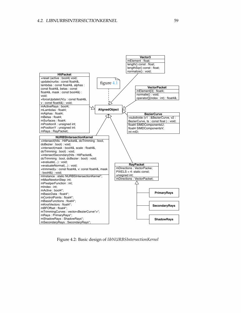
4.2. LIBNURBSINTERSECTIONKERNEL 59
Bezier&urve!subdivide (v1 , -Be/ierCurve, v2 , Be/ierCurve, ts , const 8oat ) , void;8oat4 SIMDComponentsU;8oat4 SIMDComponentsV;int mID;
AlignedOb0ect
3ector3mElement , 8oat;length() const , 8oat;lengthSIr() const , 8oat;normali/e() , void;
3ectorPacketmElement[3] , 8oat4;normalie() , void;operator[](index , int) , 8oat4-;
RayPacketmDirections , VectorPacke;PIPELS = 4, static const; unsigned int;mDirections , VectorPacket;
PrimaryRays
=econdaryRays
=hado?Rays
HitPacket!reset (active , bool4) void;update(nurbs , const 8oat4-, lambdas , const 8oat4-, alphas , const 8oat4-, betas , const 8oat4-, mask , const bool4-) , void;!forceUpdateUV(u , const 8oat4-, v , const 8oat4-) , void;mActiveRays , bool4;mLambdas , 8oat4;mAlphas , 8oat4;mBetas , 8oat4;mSurfaces , 8oat4;mPositionP , unsigned int;mPositionW , unsigned int,mRays , RayPacket;
NBRB=CntersectionDernel!intersect(hits , HitPacket-, doTrimming , bool, doBe/ier , bool) , void;!intersect(mask , bool4-, scale , 8oat4-, doTrimming , bool) , void;!intersectSecondary(hits , HitPacket-, doTrimming , bool, doBe/ier , bool) , void;!evaluate(...) , void;!evaluateNormal(...) , void;!trimmed(u , const 8oat4-, v, const 8oat4-, mask , bool4-) , void;mInstance , static NURBSIntersection\ernel];mMaxNewtonStep, int;mPixelperFunction , int;mIndex , int;mActive , bool4];mBasicData , 8oat4];mControlPoints , 8oat4];mBasisFunctions , 8oat4];m\notVectors , 8oat4];mBFOffset , 8oat4];mTrimmingCurves , vectoraBe/ierCurve]b];mRays , PrimaryRays];mShadowRays , ShadowRays];mSecondaryRays , SecondaryRays];
figure 4.1
Figure 4.2: Basic design of libNURBSIntersectionKernel

60 CHAPTER 4. STANDALONE LIBRARIES
Algorithm 5: NURBSIntersectionKernel evaluation function calls
NURBSIntersectionKernel *ik = NURBSIntersectionKernel::Instance();
//configure the kernel with all necessary data
float4 u = simd_set(0.0f, 0.33f, 0.66f, 1.0f);//sets all four values to 0.5float4 v = simd_set(0.5f);
//these will store the resultsfloat4 resX, resY, resZ;
//normal evaluation of surface pointsevaluate(u, v, false, false, resX, resY, resZ);
//evaluation of partial derivative in v directionevaluate(u, v, false, true, resX, resY, resZ);
//evaluation of normalsevaluateNormal(u, v, resX, resY, resZ);
• cfgTrimmingCurves(vector<bezierCurve*>* const curves)
The evaluation call needs two float4 vectors containing the u and v parame-ter values, two boolean values indicating if partial derivatives in u and/orv direction shall be computed and finally three float4 vectors, which willstore the results. The following example shows the appropriate call forcomputing four points on the surface, as well as the command for comput-ing the partial derivative in v parametric direction. Computing the normals(i.e. evaluateNormal()) is nearly the same command, only the boolean val-ues for the derivatives do not need to be specified. However, a booleanflag as last parameter switches between NURBS and Bézier normal evalu-ation. The default value is false, i.e. by not providing this value the NURBSvariant will be used. Basically the computation of the normals is a crossproduct of the partial derivatives, i.e. SuxSv where Sdir denotes their par-tial derivative in dir parametric direction. Again, for a complete overviewon all related configure and computation instructions for both NURBS andBézier, have a look at appendix A.

4.2. LIBNURBSINTERSECTIONKERNEL 61
4.2.2 Intersect Methods
There are three different intersection methods, one each for primary rays,secondary (i.e reflected) rays and shadow rays. The required configurationcommands for NURBS surfaces are as follows
• cfgIndex(const int index)
• cfgActiveComponents(bool4 const active)
• cfgBasicDataVector(float4* const basicData)
• cfgBoxMinMaxUV(float4* const minU, maxU, minV, maxV)
• cfgSurfaceMinMaxUV(float4* const minMaxUV)
• cfgControlPoints(float4* const controlPoints)
• cfgKnotVectors(float4* const controlPoints)
• cfgBasisFunctions(float4* const basisFunctions)
• cfgBFOffset(float4* const offset)
• one of these:
– cfgRays(PrimaryRays const* rays);
– cfgRays(ShadowRays const* rays);
– cfgRays(SecondaryRays const* rays);
• optionally: cfgTrimmingCurves(vector<bezierCurve*>* const curves)
For Bézier surfaces this effectively reduces to
• cfgIndex(const int index)
• cfgActiveComponents(bool4 const active)
• cfgBoxMinMaxUV(float4* const minU, maxU, minV, maxV)
• cfgControlPoints(float4* const controlPoints)
• one of these:
– cfgRays(PrimaryRays const* rays);
– cfgRays(ShadowRays const* rays);
– cfgRays(SecondaryRays const* rays);
• optionally: cfgTrimmingCurves(vector<BezierCurve*>* const curves)

62 CHAPTER 4. STANDALONE LIBRARIES
Note: The trimming curves for both variants are optional, but if no trim-ming test should be performed, the kernel has to be configured by provid-ing a NULL argument. If this is ignored, the old value will be kept and used!
After successful configuration of the kernel, the appropriate intersectionmethod (depending on the rays provided) can be called. The interface forthe intersection test for primary and secondary rays is identical. However,the shadow test interface differs, since it is uninteresting to know the exacthit location, but only if the rays were hitting anything or not.
//Primary intersection testvoid intersect(HitPacket& hits);
//Secondaryvoid intersectSecondary(HitPacket& hit);
//Shadowvoid intersect(bool4& mask, float4&scale);
The HitPackets will store all information related to the found intersectionpoints, that is, the unique identifiers of the hit surfaces as well as the u andv parameter values and the distances from the hit points to the origin of therays.
Whereas the mask parameter will only store wether a surface was hit atall or not, which means if a specific point in space is shadowed or not. Thescale parameter can be used during transparency calculations.

Chapter 5
Application crianusurt
This chapter is about the actual rendering application crianusurt. Althoughthe intersection and trimming tests are implemented within libNURBSInter-sectionKernel, they belong logically to this application and thus are describedin section 5.2 and section 5.4. Some in depth considerations about the mem-ory consumption can be found in section 5.5 and section 5.6 concludes thischapter with problems and limits of ray tracing NURBS.
5.1 Basic Architecture
Detailed information about the basic architecture can be found in the dis-sertation of Markus Geimer [12]. Figure 5.1 shows the topmost architec-tural design of the original application dream which basically also appliesto crianusurt. The biggest differences are to be found in the PrimaryThreadand ShadingThread. The functionality to trace and shade triangles was re-placed by the appropriate parts of libNURBSIntersectionKernel. Most otherparts of the system needed only minor adaptions or none at all. The fol-lowing sections will give an overview of the new concepts which extendedor replaced important parts of the original application dream.
5.2 Intersection Test Ray-NURBS Surface
One of the most important tasks of a ray tracer is, not surprisingly, the in-tersection test of rays and scene objects, which are NURBS and Bézier sur-faces only in this implementation. Depending on the scene, as well as cam-era position, roughly 30% to 60% of the computation effort is spend in theray-surface intersection test. A major part is spent traversing the bound-ing volume hierarchy where the rest will be used for shading, generatingnew rays, composing the final image and so on. The bounding volume hi-erarchy traversal was already highly optimized in dream, which leaves the
63
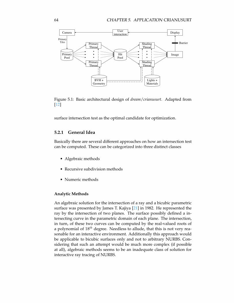
64 CHAPTER 5. APPLICATION CRIANUSURT
Figure 5.1: Basic architectural design of dream/crianusurt. Adapted from[12]
surface intersection test as the optimal candidate for optimization.
5.2.1 General Idea
Basically there are several different approaches on how an intersection testcan be computed. These can be categorized into three distinct classes
• Algebraic methods
• Recursive subdivision methods
• Numeric methods
Analytic Methods
An algebraic solution for the intersection of a ray and a bicubic parametricsurface was presented by James T. Kajiya [21] in 1982. He represented theray by the intersection of two planes. The surface possibly defined a in-tersecting curve in the parametric domain of each plane. The intersection,in turn, of these two curves can be computed by the real-valued roots ofa polynomial of 18th degree. Needless to allude, that this is not very rea-sonable for an interactive environment. Additionally this approach wouldbe applicable to bicubic surfaces only and not to arbitrary NURBS. Con-sidering that such an attempt would be much more complex (if possibleat all), algebraic methods seems to be an inadequate class of solution forinteractive ray tracing of NURBS.

5.2. INTERSECTION TEST RAY-NURBS SURFACE 65
Recursive Subdivision Methods
One of the most common ways NURBS surfaces have been ray traced so far,was by actually avoiding the direct intersection test with NURBS surfacesat all. Nearly every ray tracing application computes only the intersectionbetween rays and triangles, thus the idea is to triangulate the surfaces in away that they are very close to the original shape defined by the NURBSsurface. Again there are different approaches, but basically the choice iswether to triangulate in a preprocessing step or to triangulate during run-time on the fly. These Subdivision Surfaces are better known in their variantsintroduced by Catmull-Clark in [11] or Loop in [23], for example.
The other approach is easier to implement, but surely will suffer from theusual issues polygonial representations have, i.e. visible polygon edgeswithin a surface, high memory consumption and the like. Additionally forhigh resolution models, like they are used in the automobile industry forexample, the preprocessing step for triangulation can take up to a wholeday (which also makes an good triangulation during runtime impossible).Finally, this work is about rendering real parametric free form surfaces andthus avoiding the problem by triangulating them is not an option1.
Numeric Methods
Whenever an analytical solution is not available or not applicable, it is agood idea to consider employment of numeric methods. The Newton Iter-ation has proven itself very successful for the rendering of Bézier surfaces(see [1]) and the same basic algorithm can be applied to NURBS surfaces aswell. The idea is outlined in the next section.
5.2.2 Newton Iteration
Newton’s iteration (see [29] further details) , also called Newton-Raphsonmethod, is often used in a 2D environment, for instance to compute the rootof a function. It is very popular because of it’s (most of the time) quadraticconvergence, as well as an very easy and fast implementation. The draw-back is, that an initial guess is required to start the iteration with. Thisvalue has to be close to the real root. How close a guess has to be, is de-pendent on the function, i.e. a high degree function with large coefficientsmost likely needs a closer guess than a simple quadratic function2. Anotherdrawback is, that the first derivative is also required as well. Equation 5.1shows Newton’s iteration for the 2D case. In spite of these drawbacks theNewton Iteration seems like an ideal candidate, since the first derivative
1Additionally triangles are currently not supported in this version2For linear functions the starting guess does not matter at all

66 CHAPTER 5. APPLICATION CRIANUSURT
is relatively easy to compute (see 2.2.9) and a good starting value can beensured by the bounding box hierarchy (see 3.2.2)
xn+1 = xn #f (xn)f $(xn)
(5.1)
Assuming a good starting value, every iteration will bring the result closerto the real root, effectively reducing the error quadratically, except when-ever f $(xn) = 0 holds, in which case the error only reduces linearly.
Obtaining a good initial guess is one of the major problems when employ-ing the Newton iteration. As mentioned before, in this work the boundingvolume hierarchy will provide the initial starting value. For launching theIteration the median of the bounded parametric domain of the last bound-ing box that was tested, will be used. This approach was first proposedin [26]. Another method was introduced by Hanan Samet in [27], wherethe Oslo algorithm (refer to 2.2.6 if necessary) was used to subdivide thesurface, until the real surface was approximated closely. An intersectionwith the control point net then yielded the initial guess. The oslo algorithmis employed in iges2dsd as well during pre-precoessing, however, such anapproach, used during rendering, is much to expensive regarding requiredcomputation effort.
Other numerical approaches, like the secand method or Banach fix-point theo-rem among others, would also be more or less employable, but all of themare not really as qualified as the Newton iteration is. The secand method forinstance looks well suited in the first place, since no evaluation of the firstderivative is needed and with a fixed point approach (i.e. secand methodfirst order) only one evaluation of the surface after the first iteration (requir-ing two evaluations) would be needed, but the convergence rate is linearonly. The same applies basically for the fix point theorem. For the latter asingle iteration step is additionally far more complex compared to the New-ton iteration. Considering this, it can be assumed that both approaches willperform significantly slower, but still a further investigation on that in thefuture might be interesting.
5.2.3 3D Extension to Newton’s Iteration
Since the ray tracing is performed in a three dimensional environment, theNewton Iteration needs to be extended, which renders the iteration a bitmore sophisticated. The basic idea is to represent the ray in three dimen-sional space as an intersection of two planes, as showed in figure 5.2. Wanget al. have a similar approach in [36]. However they are using the Newtoniteration only when the rays are coherent. If that is not given they employBézier clipping (as they are dealing with Bézier surfaces only) which is not

5.2. INTERSECTION TEST RAY-NURBS SURFACE 67
P1P2x
yz
n2
n1
ray
0
Figure 5.2: A ray described by the intersection of two perpendicular planesN1 and N2 as they are used for the Newton Iteration
applicable for NURBS surfaces3. William et al. are employing a similar ap-proach with respect to NURBS surfaces in [26] too, however they are nottargeting an interactive environment. Basically the implementation of theNewton iteration is akin to the works of these two groups, but the imple-mentation of the surface evaluation including the first derivative is com-pletely different, since both groups did not target interactive frame rates.
As mentioned earlier, the ray is represented by two planes. They do nothave to be orthogonal to each other, but convergence is slightly faster andmore robust if they are. In any case their normal vectors must not becollinear! The planes are represented by P1 = (N1, d1) and analogous P2 =(N2, d2), where the Ni are the normal vectors with unit length, which areperpendicular to the ray direction. The di indicate the distance to the originof the coordinate system which can be computed as follows
di = #NiO i = 1, 2
where O is the origin of the ray. Figure 5.2 shows the ray with it’s twoplanes. In order to find the intersection between a ray and the NURBSsurface the roots of equation 5.2 have to be found
R(u, v) =
(
N1S(u, v) + d1N2S(u, v) + d2
)
(5.2)
3This approach heavily relies on the convex hull properties of Bézier surfaces

68 CHAPTER 5. APPLICATION CRIANUSURT
where S(u, v) is the point on the surface at the given parameter values.The conversion of the Newton Iteration into the three dimensional variantyields the following
(
un+1vn+1
)
=
(
un
vn
)
# J#1R(un, vn)
where J is the Jacobian Matrix of R as given in in the following equation
J =
(
N1Su(u, v) N1Sv(u, v)N2Su(u, v) N2Sv(u, v)
)
(5.3)
Su(u, v) and Sv(u, v) are the partial derivatives of their corresponding para-metric direction. The inverse of the Jacobi matrix is as follows
J#1 =1
det(J)
(
J22 #J12#J21 J11
)
(5.4)
The Newton Iteration is executed until one of three termination criteria ismet. An intersection is found if, and only if, the distance (R(un, vn)) of theapproximated intersection point to the real root is below some user definedthreshold, i.e. |R(un, vn)| <$. In any other case the iteration will be contin-ued until either the distance increases from one step to the next (indicatinga possible divergence), i.e. |R(un+1, vn+1)| > |R(un, vn)| or a predefinedmaximum number of steps have been computed, which possibly could in-dicate a loop or a very slow convergence. Figure 5.3 explains the controlflow of the Newton iteration as it is implemented within this work.
Runtime Considerations
The evaluate (including partial derivatives) method is called three timesduring a single newton step and an additional evaluation is executed at theend of the intersection routine. The maximum number of iteration stepscan be set by the user, however, more than five steps are seldom neces-sary or useful at all. Although an iteration can converge after the very firstnewton step it usually takes in average around 3 to 4 steps, depending onthe complexity of the scene, the setup of the camera and the user definedparameter for a threshold that defines a valid intersection. Rays that hit asurface orthogonally, for example, are most likely converging faster thanthose that hit tangentially. For a single intersection test in average, roughly3.5 % 3 + 1 = 11.5 evaluations are necessary. Taking into account that forevery pixel most likely more than one intersection test is required and re-flections and shadows even increase this number further, it becomes clear,that several million evaluations per second are necessary to achieve inter-active frame rates (assuming an image size of 5122 pixels), which render itvery important to optimize this method to the maximum extend possible.

5.2. INTERSECTION TEST RAY-NURBS SURFACE 69
Figure 5.3: Control flow diagram of the intersection method. This diagramis applicable for any kind of rays, however, for computing shadow rays afaster approach has been implemented as it is sufficient to know if there is ahit point at all, rather than knowing the exact point. Evaluate resp. partialderivative are shown in figure 5.4

70 CHAPTER 5. APPLICATION CRIANUSURT
5.2.4 Evaluation of Surface Points
Every performance improvement during the surface evaluation will speedup the whole application significantly. As mentioned in section 3.4.3, themost efficient way is to pre-compute the basis functions and evaluate merepolynomials instead of the Cox-de Boor recursion. Depending on wetherSIMD and/or GPU are used or not, the way of evaluating these polynomi-als will be different. Basically the same method with some modificationscan be used for either evaluating a point on a surface or the partial deriva-tive in u or v parametric direction.
The issue here is, that the derivative of a B-Spline Surface is rather simple,but when considering real NURBS surfaces, that have weights assigned tothem, the derivative is becoming a bit more sophisticated to compute, sincethe quotient rule has to be applied. However, most of the time all weightswill be one, because as mentioned earlier, the rational part of NURBS isnot used very often4. Because of that several modules where implementedwhich will suit different purposes.
• highperf_nonrational: Offers the fastest evaluation of non-rational B-Spline surfaces (weights are all considered to be one, even if they arenot) by using pre-computed basis functions as described in 3.4.4
• highperf_rational: Same as above, but adding support for rationalsurfaces as well. This variant is slower then the non-rational variant(see section 7.2 for comparison)
• baseline_nonrational: Also for evaluating non-rational B-Spline sur-faces, but by using the most straightforward approach as shown insection 3.4.1. This module is usable for benchmarking and compari-son.
• baseline_rational: Same as above with rational surface support
Because even a single if condition (to check wether the surface is rationalor not) will be expensive when employed in the most inner loop, it is alsopossible to compile the rational module completely out, for a maximum ofperformance.
Figure 5.4 shows the general control flow chart of the evaluate method.It is more explained in detail in the following section.
4For instance, even Alias’ Maya is not able to modify weights by default. This is onlypossible by writing a script

5.2. INTERSECTION TEST RAY-NURBS SURFACE 71
Figure 5.4: Control flow diagram of the evaluation method. Special atten-tion has to be paid to the shifting values to access the correct pre-computedbasis functions
Evaluating using SIMD
Basically the evaluation of a point on a NURBS surface is the result of equa-tion 2.10 for any given u and v parameter value pairs. For non-rationalsurfaces this reduces to:
S(u, v) =n+1
∑i=1
m+1
∑j=1
Bi, jNi,k(u)Mj,l(v)
The biggest different to a straight forward approach is probably the correctaccess and evaluation of the pre-computed basis functions. Every NURBSsurface stores a pointer to the first basis function, which is describing thefirst knot vector interval in u parametric direction. Refer to section 3.5.1 fora more detailed discussion about that.
However, there are some issues when employing SIMD instructions withpre-processed basis functions. Recall, that always pairs of four values areprocessed in parallel. The basis functions are dependent on the current u orv parameter values, which means, that it can occur, that two or more differ-ent basis functions have to be used for a single evaluation. This can not bedone efficiently in parallel, thus it has to be done sequentially. In the worstcase this can result in four sequential evaluations, if all values within a sin-gle SIMD vector lie in different knot vector intervals. However, as the raysare usually more or less coherent, all lie most of the time within the sameinterval or seldom in two adjacent intervals when the rays are crossing aboundary. Still, the worst case is simply comparable to FPU computation.

72 CHAPTER 5. APPLICATION CRIANUSURT
Furthermore there is another issue with the way data is stored in SIMDregisters. It is not possible to randomly access single components of oneSIMD register, as the specific access to a single of the four float compo-nents has to be known at compile time, as mentioned before. In orderto be able to use the efficient Horner scheme to evaluate the basis func-tions, the data has to be copied (i.e. splatted) into SIMD vectors. Forexample the SIMD vector a = {1, 2, 3, 4} will be copied into four vectorsv1 = {1, 1, 1, 1}, v2 = {2, 2, 2, 2} and so on. In the former case, random accessto the individual components of a during runtime is not possible, where vi
can be accessed at will, of course. The following code snipped shows theSIMD code for Horner’s scheme
float4 result = data[0];result = simd_madd(data[0],t,data[1]);float4* dp = &(data[1]);for (int i = 1; i < degree; i++)
result = simd_madd(result,t,*(++dp));
where t denotes the parameter value which is employed and data is anarray of flaot4 vectors holding the splatted values as described above. Note,that if the derivative is requested, the data array is modified accordinglyand the degree is reduced by one beforehand.
Evaluating using the GPU
On the GPU the polynomials are evaluated by using brute force, that is bysimply using the pow() built-in function. Usually this would not be veryclever, since raising to the power of an arbitrary number is extremely ex-pensive to compute and thus can not compete in any way to the Horner’sscheme used on the CPU. However, due to it’s graphics centric architecture,the GPU lacks some important abilities, like dynamic access on an arrayduring runtime (i.e. the access index has to be determined during compiletime), similar to the component access of a SIMD vector. ImplementingHorner’s scheme on the GPU is only possible with a considerable amountof workarounds, which would drop performance significantly. Luckily thepow() command does not mean a performance loss on the GPU, as it ismapped to a hardware function and thus brute force evaluation is not onlynecessary but also reasonable.
Algorithm 6 shows the corresponding GLSL code for evaluating basis func-tions. PIXELPERFUNCTION denotes the constant, which specifies howmany pixels are used to store the basis function. Furthermore, basisFunc-tions is a global shader constant referring to the texture storing all basisfunctions and accessU/accessV denote the coordinates where to find the cor-rect basis function.

5.2. INTERSECTION TEST RAY-NURBS SURFACE 73
Algorithm 6: Function evaluation on the GPU
float evaluateBasisFunctionFloat4(const float accessU, const float accessV,const float t, const int PIXELPERFUNCTION){
float result = 0;//this is the first pixel storing the degree in its first//component and the three coefficients with the highest//degreeconst vec4 p = texture2DRect(basisFunctions,
vec2(accessU, accessV));const int degree = p.x;
//independent of the degree the first pixel will always//be read and processed. Note that components might be//zero if they are not used and thus do not influence//the resultresult = p.y*pow(t, degree)
+p.z*pow(t, max(degree-1,0.f))+p.w*pow(t, max(degree-2,0.f));
//process more pixels depending on the degreefor (float i = 1; i < PIXELPERFUNCTION; i++){//read next pixel, storing four more coefficients
const vec4 p = texture2DRect(basisFunctions,vec2(accessU+i, accessV));
result = result + p.x*pow(t, max(degree-(i*4+1),0.f))+ p.y*pow(t, max(degree-(i*4),0.f))+ p.z*pow(t, max(degree-(i*4-1),0.f))+ p.w*pow(t, max(degree-(i*4-2),0.f));
}return result;
}

74 CHAPTER 5. APPLICATION CRIANUSURT
5.3 Intersection Test Ray-Bézier Surface
As mentioned before, bicubic Bézier surfaces are also supported, as a highperformance alternative to NURBS surfaces. An in depth discussion wouldexceed the scope of this work, thus in the following only a short summarywill be presented. Refer to [1] for more details, if desired.
The main difference between NURBS and Bézier surfaces during the inter-section test lies principally in the evaluation of points and partial deriva-tives only. Everything else, like the Newton Iteration and bounding volumehierarchy is fully compatible and fortunately works in the very same way.The bicubic Bézier representation is a lot faster than NURBS (see section 7.6for results), however, it is not as flexible, since such a surface always has 16control points and a cubic degree in both parametric directions. The perfor-mance advantage is mostly due to a very powerful matrix representationof the surface. Every bicubic Bézier surface can be expressed as a matrixproduct
P = UNBNV
where for bicubic patches
N =
*
+
+
,
#1 3 #3 13 #6 3 0
#3 3 0 01 0 0 0
-
.
.
/
Furthermore U is a matrix composed of the potencies of the parametervalue u, where the surface shall be evaluated
U =0
un un#1 ... u 11
analog to that
V =
*
+
+
+
+
+
,
vn
vn#1
...v1
-
.
.
.
.
.
/
Finally B is the control point matrix, i.e. every component holds a con-trol point, thus a three component vector. Note that the inner product ofP = NBN can be pre-computed, yielding a single 4 & 4 matrix with 3D vec-tor components. The necessary computation during runtime is only theproduct of three matrices, i.e. UPV, which is, compared to the operationsrequired for NURBS, rather simple.

5.4. TRIMMING TEST 75
The partial derivatives are also easy to compute. The derivative in u di-rection requires only U to be derived thus straightforward yielding
U$ =0
3u2 2u 1 01
Derivative in v direction is analog.
5.4 Trimming Test
A trimming test has to be performed, if at least one ray in a RayPacket hashit a surface and the bounding box, which started the Newton iteration,has the doTrimming flag set (compare section 3.3.1 on pre-classifying). Ob-viously, rays intersecting a non trimmed surface report their hits imme-diately, without performing any trimming operations. Rectangular para-metric regions, which are always trimmed have been removed during thepreprocessing (see 3.3.1) and thus can not be hit at all.
As mentioned earlier in section 3.3.2 trimming curves are required to beclosed. If that is assured then the following method can be applied to testwether a specific point lies within a trimmed region or not.
By shooting a 2D ray (in the parametric domain) in any direction, it is possi-ble to count the number of intersections with trimming curves. If this num-ber is odd, then the point from where the ray was casted, is enclosed bytrimming curves (i.e. trimmed) otherwise the point is not trimmed. Figure5.5 gives an example. Although this sounds very simple, it is still necessaryto make it run efficient and fast, for example, it is not reasonable to cast aray and perform real full featured ray tracing in 2D. An efficient solution ispresented in the next section.
5.4.1 Classification of Hit Points
The following technique for fast hit point classification is based on an ideainitially proposed by Nishita in [39], called Bézier Clipping, which got mod-ified to suit the needs of interactive ray tracing.
First of all, Nishita is proposing to cast a ray in a direction, that the dis-tance to the border of the parametric domain will be minimized. However,seems not reasonable in this context, as the computation to find the shortestaxis itself takes a few cycles and after all it potentially does not really re-duce the number of curve segments that have to be tested. Additionally thealgorithm would get more complicated, as it would have to handle moregeneral cases, so it is actually more feasible to cast the ray always along oneparametric direction, which is the positive u axis here (although any other
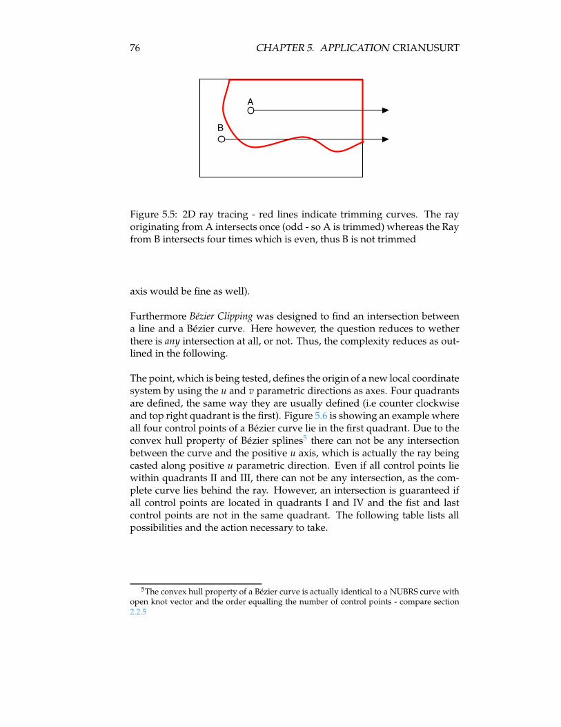
76 CHAPTER 5. APPLICATION CRIANUSURT
Figure 5.5: 2D ray tracing - red lines indicate trimming curves. The rayoriginating from A intersects once (odd - so A is trimmed) whereas the Rayfrom B intersects four times which is even, thus B is not trimmed
axis would be fine as well).
Furthermore Bézier Clipping was designed to find an intersection betweena line and a Bézier curve. Here however, the question reduces to wetherthere is any intersection at all, or not. Thus, the complexity reduces as out-lined in the following.
The point, which is being tested, defines the origin of a new local coordinatesystem by using the u and v parametric directions as axes. Four quadrantsare defined, the same way they are usually defined (i.e counter clockwiseand top right quadrant is the first). Figure 5.6 is showing an example whereall four control points of a Bézier curve lie in the first quadrant. Due to theconvex hull property of Bézier splines5 there can not be any intersectionbetween the curve and the positive u axis, which is actually the ray beingcasted along positive u parametric direction. Even if all control points liewithin quadrants II and III, there can not be any intersection, as the com-plete curve lies behind the ray. However, an intersection is guaranteed ifall control points are located in quadrants I and IV and the fist and lastcontrol points are not in the same quadrant. The following table lists allpossibilities and the action necessary to take.
5The convex hull property of a Bézier curve is actually identical to a NUBRS curve withopen knot vector and the order equalling the number of control points - compare section2.2.5

5.4. TRIMMING TEST 77
Figure 5.6: Point A is tested for trimming. A ray is cast originating fromA along positive u axis. All control points of this trimming curve lie inquadrant I thus there can not be an intersection due to the convex hullproperty
Control pointsAll in I no Intersection -> next CurveAll in II no Intersection -> next CurveAll in III no Intersection -> next CurveAll in IV no Intersection -> next CurveAll in I & II no Intersection -> next CurveAll in II & III no Intersection -> next CurveAll in III & IV no Intersection -> next CurveAll in I & IV q(p1) '= q(p4) & Intersection -> invert in/out statuselse undefined -> subdivide curve & repeat for both
It becomes obvious, that in most cases the classification for a single curvesegment is already done after a single step. Only if a curve, for example, ispassing quadrants I, II and III a subdivision is necessary, in order to solvethe problem for both smaller curves. As mentioned before, a hit is guar-anteed, if the first and last control point lie in quadrants I and IV, but notwithin the same, whereas the other two have to be in I and IV as well. Inthat case it is actually only known, that there is an intersection at all, but it isunknown how many. However, as trimming curves have been restricted tocubic degree in the beginning, it can be either one or three intersections andthis in turn does not play any role for the trimming test, because it is onlyinteresting to know, wether there is an even or odd number of intersections.In the case of cubic curves it is always an odd number of intersections, ifthere is any at all. Thus, whenever any intersection occurs, it is sufficient toflip a boolean value indicating if the point is trimmed or untrimmed.
However, if none of the definite cases is applicable, the curve has to besubdivided, since it is not possible to decide the problem on basis of thiscurve. Nishita introduces in [39] an approach with which it is possible to

78 CHAPTER 5. APPLICATION CRIANUSURT
divide the curve into three segments, where two of them are assured to beone of the definite cases and the third (i.e. middle) segment comes underanother scrutiny. Tests have shown that in the context of interactive raytracing it is more efficient to employ a rather brute force approach, whichsimply subdivides the curve in the parametric center. Otherwise, followingNishita’s approach, it would be necessary to compute two subdivision pa-rameters which is considerably expensive on its own. Theoretically it canhappen that an (nearly) endless loop of subdivisions occur, but this is mostunlikely anyway, so that a proper solution to that problem is to simply in-terrupt subdivision after, for example, 25 steps. Tests have shown that thishappens with a probability of less than 10#8% and even then it only resultsin up to four wrong pixels for one frame.
As mentioned before, a trimming curve is actually composed of a num-ber of segments. Each segment has to be tested individually as describedabove, however, the boolean flag storing the trimming status (i.e. in or out)has to be carried over, of course. After all trimming curves segments havebeen processed sequentially, the boolean flag indicates the final status ofthe point that was being tested.
5.4.2 Subdivision of Trimming Curves
Obviously two important requirements for trimming curve subdivision areperformance as well as accuracy (i.e. the two resulting curves concatenatedshould be identical to the original one). As only cubic curves are consid-ered, the well known de Casteljau algorithm [6] is perfectly suited for thatpurpose. The idea is outlined in the following.
In order to subdivide a Bézier curve of arbitrary degree at some parametervalue t with 0 " t " 1, it is necessary to recursively compute the vectorsbetween two neighboring points. These will be scaled by factor t and thewhole process is repeated for the resulting points until only one point isleft, which is the point on the curve at that parameter value. In every stepthe number of resulting points is reduced by one, thus when subdividingcubic curves, three steps are necessary, which is still quite reasonable, butmight be too costly if higher degree curves were considered. The interest-ing thing is, that the intermediate points, that were computed during theprocess, are the new control points for the two refined curves, which makesde Casteljau’s algorithm very valuable.
For the following example points Pi denote the control points of the originalcurve, where Ai and Bi refer to the two curves resulting after subdivision(0 " i " 3). Figure 5.7 is showing a simple example where a curve is sub-divided at t = 0.75. It is known, that the first and last control point of a

5.4. TRIMMING TEST 79
A0
A1
A2
A3/B0
B1
B2
B3
Figure 5.7: de Casteljau’s algorithm for a cubic spline being evaluated att = 0.75
Bézier curve lie always on the curve itself, furthermore the point evaluatedat t is also to be known on the curve and so is the value, where the two areactually connected to each other. Thus for the new segments A and B, it isalready know that
A0 = P0A4 = evalB0 = evalB3 = P3
where eval denotes the evaluated point (i.e. A3/B0 in figure 5.7). The otherfour missing control points (two per curve) are, as mentioned, the interme-diate results of the de Casteljau algorithm.
A1 = t % (P1 # P0)A2 = t % (t % (P2 # P1)# A1)B1 = t % (P3 # P2)B2 = t % (t % (P2 # P1)# B1)
Note again, that only cubic curves are considered, so it is possible to imple-ment a SIMD powered subdivision algorithm which due to some necessaryoverhead is not optimally fast, but still faster than an implementation us-ing the FPU. For example in the first step of the algorithm it is possible tocompute all vectors from Pi to Pi+1 with (0 " i " 2) in parallel using SIMDinstructions which is illustrated in figure 5.8. In the next two followingsteps the parallelism is reduced by one each time.

80 CHAPTER 5. APPLICATION CRIANUSURT
Control Points P
Vector Shift Right SR
p0 p1 p2 p3
0 p0 p1
p1#
p0
p2#
p1
p3#
p2
p2
Result
Figure 5.8: First step of the de Casteljau algorithm using SIMD
5.5 Memory Consumption
Memory consumption for a single patch is obviously higher than for a tri-angle, but overall memory usage can compete against triangular meshesquite well, especially if those are of high resolution. As mentioned before, asingle free form surface can describe a shape that would have been approx-imated by several thousand triangles otherwise, if a high resolution rep-resentation is desired. The following tabular lists the memory needed byeach object type and their components. The abbreviations used are: ControlPoints (CP), Knot Vectos (KV), Basis Functions (BF) and Trimming Curves(TC).
Object Memory (bytes)NURBS patch 104+CP+KV+BF+TCBézier patch 224 + TCCP 16 per VertexKV max(degreeU + countU + 1, degreeV + countV + 1) % 16BF c % PIXELPERFUNCTION % 16 (for c see 3.1)TC #Curves * 32Bounding Box 52NURBSKernel 92Triangle6 48
The following example shows the memory consumption for the NURB-Shead scene. The head consists of 915 NURBS surfaces, each having 4 & 4control points, degree 3 in both directions, yielding [0 0 0 0 1 1 1 1] asthe knot vectors. This will result in eight basis functions per patch, requir-ing two float4 vectors per function. Furthermore 13842 bounding boxes aregenerated and no trimming curves are used. Memory consumption there-fore is
6as used in dream

5.6. PROBLEMS AND LIMITS 81
• NURBS surfaces: 95160 bytes
• Control Points: 234240 bytes
• Knot Vectors : 117120 bytes
• Basis Functions: 234240 bytes
• Bounding Boxes: 719784 bytes
The total memory consumption for this scene is only around 1.33 MB fora virtual unlimited high resolution model. Comparing this to a trianglebased ray tracer and assuming the same memory usage for the boundingvolume hierarchy, around 680 KB would be left for triangle storage. This isenough to store more than 14000 triangles. With that number of trianglesthe head could be modeled, of course, but it might not be sufficient for highdetailed close up shots.
If the same scene would be represented as Bézier surfaces instead of NURBSthe memory consumption is reduced further to only 1.04 MB (0.83 MB forbounding boxes) would be needed, leaving only an equivalent of 4270 tri-angles, which is really not sufficient for a sophisticated head model.
5.6 Problems and Limits
NURBS surfaces can easily become very complex. Naturally there are somelimits within which the interactive ray tracing of NURBS surfaces is feasi-ble and reasonable.
In section 7 it is shown, that it is possible to render thousands of NURBSsurfaces with interactive frame rates, even on a single modern commodityPC. However, this requires that the surfaces are within a certain reasonablerange. On the one hand, the baseline algorithm can render any complex-ity, but interactive frame rates are out of sight pretty fast, whereas on theother hand, the highperf algorithm keeps it’s speed quite well, but loosingaccuracy pretty fast, because of the limited precision of floating point val-ues. One possible workaround is to use double precision when enablingthe FPU emulation mode, however this of course is reducing performancea lot, as well. A possible solution to that problem is outlined in chapter 8.
5.6.1 Insufficient Floating Point Precision
Numerical inaccuracy becomes a serious problem, when there are a largenumber of control vertices with a low or medium degree of the basis func-tions. The reason is, whenever this situation occurs, a great number of basis

82 CHAPTER 5. APPLICATION CRIANUSURT
functions has to be generated, which each cover only a very small regionof the parametric domain, This in turn means, that their coefficients willbecome rather large. Unfortunately single precision floating point values(after IEEE-754 [37]) are only able to store seven different figures. The fol-lowing example shows two of the basis functions, that are used in the asimple B-Spline Patch, taken from [34], but instead constructed out of 132
control vertices with degree 5 in each parametric direction.
Ms9,5(v)0.875<v"1 = 3117.51v5 # 14734.2v4 + 27761.8v3
# 26055.1v2 + 12174.2v # 2264.18
Ms11,5(v)0.875<v"1 = 43614.8v5 # 193896v4 + 344130v3
# 304803v2 + 134803v # 23810.4
However, when these basis functions are computed using double precisionfloating point values, then the result is quite different, as follows
Md9, 5(v)0.875<v"1 = 3117, 5111111111v5 # 14734.2222222222v4
+ 27761.7777777778v3 # 26055.1111111111v2
+ 12174.2222222222v # 2264.1777777778
Md11, 5(v)0.875<v"1 = 43614.8148148148v5 # 193896.2962962963v4
+ 344130.3703703703v3 # 304841.4814814815v2
+ 134802.9629629629v # 23810.3703703704
By comparing the different coefficient values, the discrepancy between thetwo precisions become obvious. Even more serious is the fact, that thisapplies to many of the basis functions of such a surface. When evaluatinga point on the surface or a normal, then these errors accumulate, whichin turn can lead to rather inaccurate results. For example, evaluating thesurface with single precision at u = 0.95 and v = 0.95 results in
(15.1864, 1.80162,#14.681)
whereas double precision yields
(14.6165208918, 1.7701131564,#14.1254754908)

5.6. PROBLEMS AND LIMITS 83
Figure 5.9: Rendered surface with 13x13 control points and degree 5 in bothparametric directions. From left to right: Rendered with single precision(FPU and SIMD yield same result), double precision (only FPU), baseline
The absolute distance between the two different results therefor is 0.32575!
Obviously, this causes problems during the intersection tests, since the it-eration will converge to a point in space, that is not on the ray and thusthe intersection test wrongly will report a miss. An easy workaround isto soften the threshold epsilon value for intersection acceptance, howeverthis in turn may cause hits to be reported where there are none. Figure5.9 shows the mentioned cases. For very complex surfaces only the base-line variant yields a correct result, however unfortunately with far frominteractive speed. By using double precision, it is possible to handle morecomplex surfaces, but 64 bit floating point values are not supported by lib-SIMD7, so this mode is only available when using the slow FPU emulationmode. Tabular 7.3 shows the rendering times for the different methods.The rendering times for the teapot and NURBShead can also be found forcomparison. Note that both latter scenes are rendered correctly by any ofthe mentioned methods.
5.6.2 GPU Issues
It turned out, that there are some severe issues when using the graphicscard for ray tracing of NURBS, which in the end, made it not worthwhileto use it yet. The three major problems are as follows
• Limited number of temporary registers
• Limited execution length
• Performance
7SSE is supporting double precision floats with half performance, where AltiVec doesnot support it at all

84 CHAPTER 5. APPLICATION CRIANUSURT
The available amount of memory however, which seemed to be a problemin the first place, is not a real concern, unless extremely large models shouldbe rendered. Unfortunately there are currently no solid official numbersavailable, which state how many temporary registers the GeForce 6800 cardreally has nor what the limit of executed commands is. Even dedicated testsshowed an unexpected behavior by actually allowing a greater number oftemporary registers then in the intersection code. This effect is most likelydue to some optimizations in the compiler, which makes it rather hard toestimate the number of registers really being used. However, it seems thatthe following statistics are true for the GeForce 6800
• Number of constant registers: 224
• Number of temporary registers: 32
• Number of lines of executed code: 65000+
The actual problems are the number of temporary registers and the limit ofexecuted code. The latter is unlimited by hardware design, but it is in factlimited by the driver.
Temporary Registers
The effect of exceeded temporary registers is unfortunately a simple instanttermination of the application, with the error message floating point excep-tion displayed on the console, which, in the first place, does not help much.Because of this, a lot of unfavorable workarounds had to be implementedand features like trimming had to be skipped completely. Another possibleworkaround would have been a multipass approach, i.e. to render thesetemporary values into textures where they can be read again later, but thisdoesn’t even enter the equation as it is much to slow in an interactive con-text.
Execution Length
From the hardware design the GeForce 6800 can executed an unlimitednumber of commands, unless the predecessors. However, it would be un-favourable to send the graphics card into an endless loop, effectively freez-ing the screen, thus the driver does employ a limit, which seems to be 216
commands. Unfortunately this is, depending on the surface, only enoughfor one or two steps of the Newton iteration, which is simply not sufficient.Usually four or more steps are needed to obtain a result with an error be-low 10#3. Also here a multipass approach could help in theory (every stepof the Newton iteration as one pass), but as mentioned above, this wouldreduce performance considerably, making it useless in an interactive set-ting.

5.6. PROBLEMS AND LIMITS 85
Performance
Ignoring all issues encountered so far, general performance is, by far, not ashigh as necessary for interactive frame rates. Even a single surface, whichdid not even render correctly due to the mentioned problems above, tookmore than a minute, when the rendering was done on the GPU only. Com-paring these to the results achieved with the CPU solely, it is obvious that,when using them in parallel, the GPU would compute less then 1% of thepixels - and again these were even not correct results because the compu-tation could not be completed because of to the execution limit. Althoughthere might be room for runtime optimization, the complexity still remainsan severe issue.

86 CHAPTER 5. APPLICATION CRIANUSURT

Chapter 6
Usage
The usage of crianusurt is very easy, but beforehand all required librariesand applications have to be installed. Follow these commands for installingeverything needed. The given examples will work on both Linux/x86 aswell as MacOS/PowerPC.
Installing libSIMD
//change to libSIMD directory./bootstrap.sh./configure --enable-includedir=/usr/local/include/SIMDmake//change to superusermake install
Installing libNURBSIntersectionKernel
//change to libNURBSIntersectionKernel directory./bootstrap.sh./configure --enable-includedir=
/usr/local/include/NURBSIntersectionKernelmake//change to superusermake install
Installing iges2dsd/crianusurt
//change to iges2dsd/crianusurt directory./bootstrap.sh./configuremake
The order is important, as both, iges2dsd as well as crianusurt are depen-dent on libNURBSIntersectionKernel, which itself is dependent on libSIMD!
87

88 CHAPTER 6. USAGE
It is possible to append a –enable-fpu option to all configure commands,which will force the usage of the FPU emulation mode, rather than usingthe appropriate SIMD instruction set. This however, should only be usedfor speed comparisons, since it is a lot slower than the SIMD enabled vari-ant. On systems that don’t offer SIMD functionality the FPU mode will beused automatically. The option –enable-debug can be employed to gener-ate unoptimized code that can be debugged. Any of these options have tobe applied to all libraries and applications, especially applying the –enable-fpu option to only one package will prevent the other libraries/applicationsfrom working at all!
6.1 iges2dsd Usage
As discussed before, iges2dsd is responsible for converting .iges or special.wrl files into the binary .dsd format used by crianusurt. While converting,all necessary preprocessing is done, like precomputing the basis functionsand generating the bounding volume hierarchy.
The application is called by
iges2dsd [options] -i inputfile -o outputfile
Options can be any of the following
-d maximum subdividing depth during bv-hierarchy generation-w swap the y and z coordinate axis-b use the dynamic bounding volume generation (see 3.2.2)-t must be between 0 and 1. The closer to one, the more and more
exact bounding boxes will be generated[requires: -b](default: 0.85)
-c read the configuration file inputfile.cfg to sets various modelparameters (i.e. like camera, lights and scale)
The time needed for converting is usually only a few seconds. For largescenes with a lot of subdividing the process can take up to several minutes.Some preprocessing times can be found in section 7.1.
6.2 crianusurt Usage
Crianusurt is the actual rendering application. It needs a .dsd file as in-put. Besides the two libraries libSIMD and libNURBS, it also requires anOpenGL environment, which should be part of the operating system any-way. Crinsusurt is launched with
6.2. CRIANUSURT USAGE 89
crianusurt [options] -f inputfile
Options can be any of the following
-w width width of the output window (default:512)-h height height of the output window (default:512)-t num number of threads for rendering/shading (see 3.2.2)-p speed set panning speed (default:1.0)-P steps set panning steps (default:0.1)-r speed set the rotation speed (default: 10.0)-R speed set the rotation steps (default: 1.0)-e epsilon sets the epsilon value for the intersection test (Default:10#3)-n disable trimming (default: enabled)
Some of these parameters can also be changed during runtime using thefollowing keys
+ increase panning speed by panning step- decrease panning speed by panning stepShift + increase rotation speed by rotation stepShift - decrease rotation speed by rotation stepw enable/disable trimmingq increase epsilon for intersection test by factor 10Q decrease epsilon for intersection test by factor 10
Additionally there are several other keys which influence the behavior ofthe application. These are listed in the following tabular for reference
Esc terminates the applicationD increase recursion depth for secondary raysd decrease recursion depth for secondary raysb activate/deactivate benchmarking moden force rendering of new framej activate/deactivate antialias modes activate/deactivate shadowsr activate/deactivate reflectionse activate shadows and reflectionsx activate/deactivate rotation around x axisy activate/deactivate rotation around y axis
Finally you can use the arrow keys to move the camera (look-at point staysas is) and while holding shift, the arrow keys will pan the camera (look-atpoint also moves)

90 CHAPTER 6. USAGE
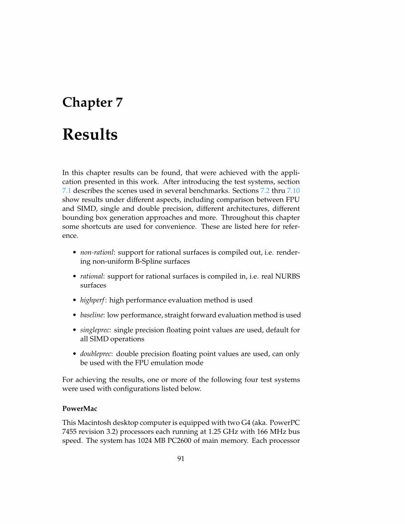
Chapter 7
Results
In this chapter results can be found, that were achieved with the appli-cation presented in this work. After introducing the test systems, section7.1 describes the scenes used in several benchmarks. Sections 7.2 thru 7.10show results under different aspects, including comparison between FPUand SIMD, single and double precision, different architectures, differentbounding box generation approaches and more. Throughout this chaptersome shortcuts are used for convenience. These are listed here for refer-ence.
• non-rationl: support for rational surfaces is compiled out, i.e. render-ing non-uniform B-Spline surfaces
• rational: support for rational surfaces is compiled in, i.e. real NURBSsurfaces
• highperf : high performance evaluation method is used
• baseline: low performance, straight forward evaluation method is used
• singleprec: single precision floating point values are used, default forall SIMD operations
• doubleprec: double precision floating point values are used, can onlybe used with the FPU emulation mode
For achieving the results, one or more of the following four test systemswere used with configurations listed below.
PowerMac
This Macintosh desktop computer is equipped with two G4 (aka. PowerPC7455 revision 3.2) processors each running at 1.25 GHz with 166 MHz busspeed. The system has 1024 MB PC2600 of main memory. Each processor
91

92 CHAPTER 7. RESULTS
has its own L1 (64 KB), L2 (256 KB) and L3 (2 MB) cache, but the bus tothe processors is shared between both. The Operating system is Mac OS X10.4.2.
PowerBook
This portable Macintosh computer sports a G4 processor running at 1.67GHz, also with a bus speed of 166 MHz. In difference to the desktop sys-tem, this is a PowerPC 7447A revision 1.2, which is optimized for mobileoperation. There is no L3 cache, the L1 cache has 64 KB of memory, whereasthe L2 cache comes along with 512 KB. The main memory is 1.5 GB ofPC2700 DDR RAM. The Operating system is the same as on the PowerMac.
PC
A desktop computer featuring a 3.0 GHz Pentium 4 processor with 1024MB of main memory. Operating system is Gentoo Linux with a 2.4.26 Ker-nel. The processor supports Intel’s hyper threading technology.
Prism
SGI’s Prism in the configuration used, features six Intel Itanium 2 64 bitprocessors each running at 1.5 GHz connected with a 400 MHz bus. Ev-ery processor has it’s own caches, that is 32 KB level 1, 256 KB level 2and 4 MB level 3 cache. Unfortunately the Itanium processor does not fea-ture a SIMD unit, thus computation has to be done using the FPU emula-tion mode. However, each processor features two full floating point units,which both are capable of computing two operations in parallel. The ma-chine is equipped with 16 GB of RAM. The operating system is Fedora CoreLinux.
G5
Another Macintosh Desktop Computer, that was used to test the perfor-mance on Apple’s newest machines. This particular one was equippedwith dual G5 (64 KB lvel1 and 512 KB level 2 cache) processors runningat 1.8 GHz, connected over a 900 MHz bus to the rest of the system. Avail-able memory was 1GB DDR RAM. Operating system is Mac OS X 10.3.9.
7.1 Test Scenes
Before going into detail, the used test scenes are shortly described. To com-pare results with each other, it matters what kind of surfaces are being ren-dered, i.e. the number of control points and the degree of the basis func-

7.2. COMPARSION: RATIONAL VS. NON-RATIONAL 93
Figure 7.1: Test scenes from left to right: parfum, head, stingray, teapot
tions that are employed. Unless otherwise stated the following parametersare always passed to the converter iges2dsd
iges2dsd -b -d 6 -t 0.85 -c [-w] -i inputfile -o outputfile
Have a look at section 6.1 for more details about the individual parameters.Note that -w (swapping Y and Z axis) is only used where needed and hasno performance impact at all. Furthermore, all results were achieved byusing two float4 values for basis function storage, effectively limiting themaximum degree to six. Also unless otherwise stated, all scenes use theimproved bounding box generation algorithm (surface flatness criterion)corresponding to the parameter -b. By default, all scenes are representedby NURBS surfaces, not Bézier!
All results shown in figure 7.1 are actually bicubic Bézier models repre-sented by uniform B-spline surfaces (unless otherwise stated). The follow-ing table states of how many patches the individuals scenes consist and alsohow many bounding boxes will be generated when using the parametersgiven above.
Scene Surfaces Bounding boxes approx. Preprocessing timeParfum 110 3090 2 sec.Head 915 13842 7 sec.
Stingray 1160 26268 14 sec.Teapot 32 12985 7 sec.
From this result it seems that the preprocessing time is heavily dependenton the number of bounding boxes generated rather than on the number ofsurfaces in a scene.
7.2 Comparsion: Rational vs. non-rational
The following results show, that the non-rational variant is more than 20%faster than the rational variant, even if all weights are 1, which effectively

94 CHAPTER 7. RESULTS
Figure 7.2: Example NURBS surface from Roger’s book (see [34]). On theleft all weights are 1, which is a simple non-rational B-Spline surface. Onthe right h4,3 is set to 5 thus defining a real NURBS surface
yields the same surface. However, especially the derivatives are computa-tionally more expensive, since the quotient rule has to be applied. Figure7.2 shows both surfaces with and without using weighting factors. Theweight h4,3 corresponds to the uppermost control vertex B4,3 and thus thesurface is pulled up towards that control point. Tabular 7.2 shows someresults. Note that the two results which have a weighting assigned at h4,3actually modify the geometry in a way, that more pixels are rendered andtested for intersections (compare the images) and thus the frame rate isslower also due to this fact.
Kind Weighting at h4,3 variant fps efficiencynon-rational no highperf 2.75 2291%
rational no highperf 2.26 1883%rational yes highperf 1.47 1225%
non-rational no baseline 0.12 100%rational no baseline 0.10 83%rational yes baseline 0.05 41%
Similar speed impacts were obtained when rendering the Utah teapot. Tab-ular 7.2 shows some more results.
Kind variant fps efficiencynon-rational highperf 1.35 2596%
rational highperf 1.01 1942%non-rational baseline 0.052 100%
rational baseline 0.043 82.6%
Note that the teapot consists of very low complex NURBS surfaces, whichare actually bicubic Bézier surfaces represented as B-Splines. However, the

7.3. COMPARISON: SIMD VS. FPU(SINGLE AND DOUBLE) 95
performance gap between the high performance and the baseline evalua-tion variants becomes even larger, the more complex the surfaces will be-come. This becomes clear in the next section.
7.3 Comparison: SIMD vs. FPU(single and double)
Theoretically the SIMD unit is four times faster than the FPU, howevermost of the times the factor is not reached due to some overhead involvedwhen using SIMD instructions. As the following results will show, in thisimplementation the computation using SIMD is even faster than four times.This can be explained by taking into account, that the FPU mode is only anemulation mode, which means that actually arrays of four rays are beingcomputed. This of course causes a certain amount of overhead. An highlyoptimized FPU based ray tracer would be able to outperform the emula-tion mode. Table 7.3 shows the results for different computation times de-pending on the method which was employed. Especially interesting is thehuge performance gap when comparing baseline and highperf computationmodes on the B-Spline Surface. Here the slow down factor from highperf tobaseline is even roughly ten times larger as the slow down that occurs withboth other scene. This is because of the more complex surface: the baselinealgorithm complexity increases super linear with every added control ver-tex whereas the highperf algorithm does not!
Comparing double and single precision, the results show that performancedrops between 25% and 40% where the latter of course is faster. This obser-vation was expected, because double precision values (i.e 64 bit length) arealways more costly to handle, especially for 32 bit processors (which theMacintosh and PC test systems are).
Method Single(13x13/5x5) Teapot NURBSheadFPU single precision 11.5s 4.5s 12.4sFPU double precision 15.5s 6.68s 19.9sSIMD basline 479s 18.6s 55sSIMD highperf 1.66s 0.74s 1.8s
7.4 Comparison: Architectures
In this section some scenes are rendered on different machines. Tabular7.4 shows the results, where the following abbreviations correspond to thetest machines described in section 7. For each system the optimal numberof threads was used to take advantage of multiple processors respectivelyhyper threading.

96 CHAPTER 7. RESULTS
Scene PowerMac PowerBook P4 G5Teapot (NURBS) 1.08 fps 0.70 fps 0.93 fps 1.09 fpsTeapot (Bézier) 3.65 fps 2.73 fps 4.56 fps 5.72 fpsSingle (NURBS) 2.28 fps 1.58 fps 2.40 fps 2.43 fpsNURBShead (NUBRS) 0.41 fps 0.27 fps 0.33 fps 0.38 fpsNURBShead (Bézier) 2.63 fps 1.87 fps 2.55 fps 3.81 fps
By comparing the results gathered by the PowerMac and PowerBook, theyare close to what is expected. Performance problems due to memory short-age can be ignored as the scenes fit into a fraction of the available free mem-ory for all systems. Ray tracing is basically a very processor intense algo-rithm as long as not the bus marks a bottleneck. Taking into account theraw processor power only, we expect roughly the following:
f pspowermac =f pspowerbook
1.336% 1.85
The difference between the processor clocks yield the factor 1.336(i.e 1.67GHz
1.25GHz), where 0.85 is the assumed scalability factor for dual proces-sors (see also next section 7.7). For the teapot in NURBS representationthis means: 0.70/1.336 % 1.85 = 0.969 which is quite close to the actuallyachieved 1.08 fps. The small difference might be due to architectural dif-ferences in both processors or similar reasons.
However, comparing the results on the PC with those achieved on a Mac,some unexpected surprises arise. The results for the teapot in NURBS rep-resentation are actually what is expected. The 3 GHz Pentium IV performs32.8% better than the 1.67 GHz G4, but 13.8% slower than the dual 1.25 GHzG4. Considering, that PowerPC processors have a better GHz/Performanceratio and AltiVec is mostly superior to SSE the result seems to be reason-able. However, the same scene in Bézier representation yield a differentview. In this case the Pentium outperforms both Macintoshs by 24.9% re-spectively by 67%, which might lead to the conclusion that Bézier surfacesrun faster on the x86 architecture. Unfortunately this assumption can not behold as the NURBShead in Bézier representation is actually slightly fasteron the PowerMac. The reason for that is not really clear yet. Most likely itis a combination of several reasons, like SIMD instruction set differences,clock and bus speed discrepancies as well as other causes.
By having a closer look at the G5 results even more surprises arise. Usu-ally the performance of a G5 is superior to a G4, also at (theoretically) sameclock speeds. However, the scenes in NURBS representation on both Mac-intosh desktop computers are nearly the same. Although no specific G5optimizations were employed so far for NURBS surfaces, this result seemsstrange in the first place. By taking into account that the AltiVec unit build

7.4. COMPARISON: ARCHITECTURES 97
0
0.2
0.4
0.6
0.8
1
1 2 3 4 5 6
fps
Number of processors
line 1line 2
0
0.2
0.4
0.6
0.8
1
1 2 3 4 5 6
fps
Number of processors
line 1line 2
0
0.2
0.4
0.6
0.8
1
1 2 3 4 5 6
fps
Number of processors
line 1line 2
0
0.2
0.4
0.6
0.8
1
1 2 3 4 5 6
fps
Number of processors
line 1line 2
Figure 7.3: crianusurt performance on a SGI Prism. The dashed green lineshows an ideal linear scale, where the red line shows, how the applicationscales with increasing number of processors
in G5 processors is not as powerful as compared to the G4, the resultsseem more reasonable. Looking at the Bézier representation the G5 is alot faster, which is most likely due to specific optimizations implementedin [1], where the functionality is inherited from, for this kind of processor.
The Prism was tested at the very end, upon completion of this thesis, thustime was not sufficient to fully port the application. Because of this, onlythe teapot scene was benchmarked using the FPU emulation mode, sincea SIMD unit is not available on Itanium processors. Additionally, doubleprecision was used, as single precision floating point values caused someproblems on the native 64 bit architecture. The following figure 7.3 shows,that the scalability is extremely good, but overall performance is quite poorcompared to the other test systems. The maximum frame rate that wasachieved using all six processors was 0.624 fps, which is even beaten bythe PowerBook, that reached a top speed for the same scene of 0.7 fps. Ifthe PowerBook is not using its SIMD unit and additionally also computesdouble precision values, the frame rate drops to 0.061 fps, which is nearlya factor 10 slower than the Prism. Anyway, the conclusion is, that it is alot more feasible (especially if funds are limited) to use a multi processormachine with support for a SIMD unit rather than a SGI computer.

98 CHAPTER 7. RESULTS
7.5 Comparison: Bounding Box Hierarchy Creation
As mentioned in section 3.2.2, two different variants were implemented togenerate a bounding volume hierarchy. The generation on behalf of theconvex hulls (CH) is expected to be less efficient regarding runtime andmemory consumption than the variant that creates the hierarchy based ona surface flatness criterion (FT). Table 7.5 shows the performance of bothapproaches with a different maximum subdivision depth. Additionally itis stated wether the resulting image is rendered without artifacts or not.Other test scenes yield results that do not differ much relatively, so onlythe teapot is taken as an example.
Depth Convex Hull Flatness Aftifacts (CH/FT)6 0.071 fps 0.603 fps none/none5 0.077 fps 0.604 fps none/none4 0.103 fps 0.551 fps none/none3 0.088 fps 0.594 fps none/none2 0.067 fps 0.599 fps some/some1 0.116 fps 0.613 fps many/some0 0.312 fps 0.615 fps lots/many
It is clearly visible that the FT method is superior to CH in both perfor-mance and quality. Even with a subdivision depth of 0 the FT methodis roughly twice as fast and still yielding a better result. Beginning withdepth 3, both approaches yield an artifact free result, but FT is about 6.75times faster! Overall, the FT method remains quite constant with increasingdepth, indicating that the number of bounding boxes do not have much im-pact on performance (but on image quality). Tabular 7.5 shows the numberof bounding boxes generated for both approaches.
Depth CH BB Count FT BB Count8 2604231 130677 651883 130676 164453 129815 41302 119634 10373 71003 2593 28242 623 7671 165 1950 49 195
The number of generated boxes for the CH method is constantly growing,roughly by factor four for each new subdivision step. However, FT stops

7.6. COMPARISON: DREAM, DREAMBSE, CRIANUSURT 99
growing at depth 7, which is due to the other parameter bounding the gen-eration - the flatness criterion. This indicates that according to the value(0.85 used here) all surfaces are sufficient flat enough and no further subdi-vision is necessary.
7.6 Comparison: dream, dreamBSE, crianusurt
The application crianusurt descended from dream, which provided the gen-eral SIMD ray tracer framework, and dreamBSE where the Bézier represen-tation was taken from. Naturally quite interesting is a comparison betweenthe original triangle based ray tracer dream, the Bézier based ray tracerdreamBSE and this application crianusurt. The following tests were per-formed on the PowerMac using both processors. The scene rendered is theteapot, since this is the only scene that was available for all three systemsat this point of time. Figure 7.4 shows the three results rendered by theseapplications. Note, that the result rendered by dream is a bit different, be-cause the original Bézier data could not be fed into the loader, since there isno triangulation routine for free form surfaces yet. However, the renderedplane should not make a big difference to the frame rate. The followingtable shows the frame rates for the different systems.
System Frame Rate Objects Bounding Boxesdream 1.58 fps 41050 Tris 19660dreamBSE 4.5 fps 32 Bézier 12326crianusurt 3.45 fps 32 Bézier 18875crianusurt 1.07 fps 32 NURBS 12981
The NURBS representation is not surprisingly the slowest compared toBézier and triangles, however it is only around a third slower than the lat-ter. Taking into account that generally the intersection test of ray-NURBSis far more complex than a ray-triangle test, this result is quite impres-sive. Additionally the image quality of both ray tracers is comparable.The quality of dreamBSE however, is inferior to the results rendered byusing the Bézier representation1 of crianusurt, which explains the slowerframe rate in that case. Several enhancements were implemented whichimprove accuracy during the tracing and shading, which were not inte-grated in dreamBSE yet. In figure 7.5 the difference is visible, i.e. the objectboundaries are a lot sharper in crianusurt, where the are relatively inaccu-rate in dreamBSE.
Note, that any free form surface representation uses lesser bounding boxesand only a fraction of surfaces compared to the number of triangles, thus
1crinusurt image quality is the same for Bézier and NURBS representation

100 CHAPTER 7. RESULTS
Figure 7.4: From left to right: dream, dreamBSE and crianusurt
Figure 7.5: Magnification of the teapot. The object boundary is a lot moreexact in crianusurt (right side)
memory consumption is lower for all of these. Additionally this has anpositive effect on loading time and cache performance.
7.7 Scalability
As shown in the following crianusurt is scaling quite well especially forthe NURBS representation. The application can be run with an arbitrarynumber of threads which enables support for any number of processors.For each thread an instance of the NURBSIntersectionKernel class will becreated, but this is actually not a real limit to the maximum number of exe-cutable threads, as the kernel only stores pointers to the NURBS data. Thisis easily possible, as all associated data is read-only, so there is no need toemploy locks or barriers. Every instance consumes 92 bytes of memory,assuming 4 byte long pointers. Regarding this, a few kilobytes are enoughto support more processors than anyone will be able to buy within the nextcouple of years.
The following table 7.8 shows the achieved results with three different testscenes using the default parameters for conversion and rendering.

7.8. HYPER THREADING EFFICIENCY 101
Scene 1 CPU 2 CPUs Speedup factorTeapot 0.576 fps 1.071 fps 1.85NURBS head 0.215 fps 0.416 fps 1.93Trimmed 1.100 fps 1.937 fps 1.76
The scalability for all three scenes is quite good and lies within reasonablerange, as speedup factors above 1.95 can nearly not be achieved in realworld applications due to the overhead involved when using multiple pro-cessor systems. However, the speedup factor always stays clearly above1.5 which leads to the conclusion that there is no real bottleneck involvedlike the system bus speed for example or locks in the code that prevent in-dividual threads from working. Also note the very good scaleability on thePrism in figure 7.3.
The difference in the speedup factors might be based on a lot of factors, butfrom the observed results it seems most likely, that more complex scenesscale better, which might be due to the fact of better cache performance,since more operations are performed on the same sub-surface by both pro-cessors.
7.8 Hyper Threading Efficiency
Although not a real parallel technique, Intels Hyper Threading technologyenables the processor(s) to execute two threads simultaneously. To the op-erating system a hyper threading enabled processor appears as two phys-ical processors. As there is not a second computation unit, it is really notcomparable to multi processor nor multi core systems. Basically only theI/O of the processor is optimized, thus reducing processor stalls due tocache misses for example. However, this technique is a mixed bag regard-ing performance. Of course, single threaded applications can not take anyadvantage of it, but there are also cases when performance actually de-creases when using hyper threading with multiple threads (some kinds ofvideo encoding are known for that phenomenon). Further information onIntel’s hyper threading technology can be found in [15]
The application presented in this work is optimized for cache coherency,so only a minor speed up factor is expected, as the results in tabular 7.8approve. Note, that these results were achieved with the PC system men-tioned above.
Scene HT disabled HT enabled Speedup factorTeapot 0.847 fps 0.89 fps 1.05NURBS head 0.308 fps 0.327 fps 1.061Trimmed 1.856 fps 1.870 fps 1.007

102 CHAPTER 7. RESULTS
Obviously, the performance gain is quite moderate or for the last sceneeven nearly non existent. It seems that due to the high optimization of theapplication and especially the intersection test and bounding hierarchy boxtraversal, there is not much room for hyper threading left.
7.9 Newton Iteration Accuracy
As mentioned in section 5.2.3, there are three different termination criteriafor the Newton iteration, where |R(u, v)| < $ was indicating a successfulintersection. The $ value can be chosen by the user as an application pa-rameter. The closer $ is to zero, the more accurate the actual intersectionpoint will be calculated, however, more iteration steps will be necessaryto achieve the higher precision. Additionally there is a limit to the max-imum accuracy, because of the limited precision of floating point values.Tabular 7.9 displays the effect of different $ values on render times whenusing SIMD instructions, whereas tabular 7.9 shows the improved accuracyrange by using double precision floating point values. Note that the latterrequires FPU emulation mode, thus the frame rate is a lot slower comparedto the former. Figure 7.8 shows the different results for the teapot achievedwith the SIMD enabled variant.
$ Frames/s Quality of result10#7 0.48 fps > 20% intersections missed10#6 0.93 fps < 1% intersections missed10#5 0.98 fps faultless10#4 1.03 fps faultless10#3 1.15 fps faultless0.01 1.43 fps some wrong intersections at borders0.1 2.5 fps predominant bounding box intersections( 1 3.1 fps bounding box intersections only
Figure 7.6: Results using SIMD
$ Frames/s Quality of result10#16 0.028 fps > 50% intersections missed10#15 0.059 fps < 5% intersections missed10#14 0.067 fps faultless...
......
10#3 0.085 fps faultless0.01 0.112 fps some wrong intersections at borders0.1 0.237 fps predominant bounding box intersections( 1 0.464 fps bounding box intersections only
Figure 7.7: Results using FPU emulation with double precision

7.9. NEWTON ITERATION ACCURACY 103
Figure 7.8: Different results for different $ values. The images correspondto the entries in tabular 7.9 from left to right and top to bottom. Basicallyfrom this point of view results 3 to 5 yield exactly the same result, but image5 was rendered with 1.15 fps which is around 17% faster than render timefor image 3 (0.98 fps)
Interestingly the results achieved with double precision are sill faultlesswith $ = 10#14 which is actually more than double the precision reachedwith floats, where 10#5 was the smallest value to yield correct results with.
By using double precision floating point values, it is possible to computemore exact intersections which, however, does not seem to be very worth-while, as the image quality does not benefit from smaller values than 10#5
and as mentioned in section 5.6.1 numerical problems with complex sur-faces prohibit the use of extremely small $ values anyway. Finally, as alsomentioned before, double precision is available only with the FPU emula-tion, which is rather slow. Considering this, the double precision mode isbasically only a minor extension to the range of surfaces that can be ren-dered by sacrificing performance.
Finally, the values shown here are also dependent on the scale of the scene,so that the epsilon value has to be chosen carefully for each scene. The teapotis defined in 3D space with control points values ranging roughly from -50to 200. If another scene is defined in a hundred times larger scale the $
value has to be adjusted accordingly2.
2The $ value can also be adjusted during runtime
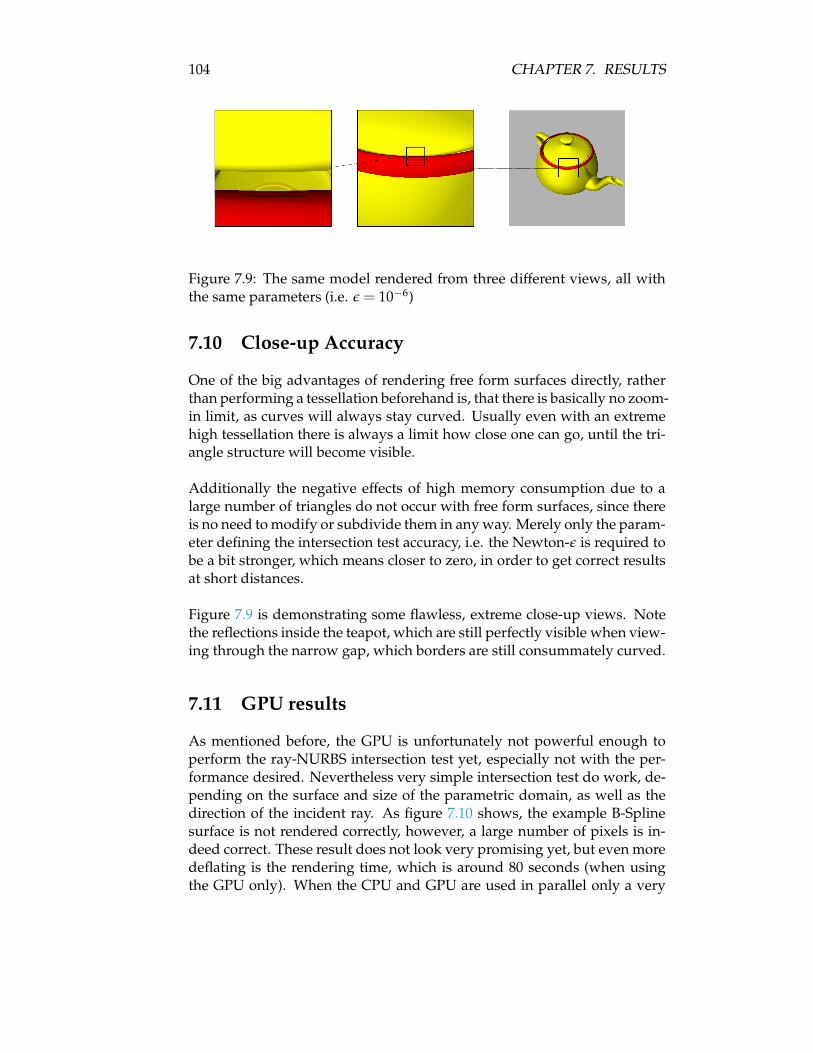
104 CHAPTER 7. RESULTS
Figure 7.9: The same model rendered from three different views, all withthe same parameters (i.e. $ = 10#6)
7.10 Close-up Accuracy
One of the big advantages of rendering free form surfaces directly, ratherthan performing a tessellation beforehand is, that there is basically no zoom-in limit, as curves will always stay curved. Usually even with an extremehigh tessellation there is always a limit how close one can go, until the tri-angle structure will become visible.
Additionally the negative effects of high memory consumption due to alarge number of triangles do not occur with free form surfaces, since thereis no need to modify or subdivide them in any way. Merely only the param-eter defining the intersection test accuracy, i.e. the Newton-$ is required tobe a bit stronger, which means closer to zero, in order to get correct resultsat short distances.
Figure 7.9 is demonstrating some flawless, extreme close-up views. Notethe reflections inside the teapot, which are still perfectly visible when view-ing through the narrow gap, which borders are still consummately curved.
7.11 GPU results
As mentioned before, the GPU is unfortunately not powerful enough toperform the ray-NURBS intersection test yet, especially not with the per-formance desired. Nevertheless very simple intersection test do work, de-pending on the surface and size of the parametric domain, as well as thedirection of the incident ray. As figure 7.10 shows, the example B-Splinesurface is not rendered correctly, however, a large number of pixels is in-deed correct. These result does not look very promising yet, but even moredeflating is the rendering time, which is around 80 seconds (when usingthe GPU only). When the CPU and GPU are used in parallel only a very
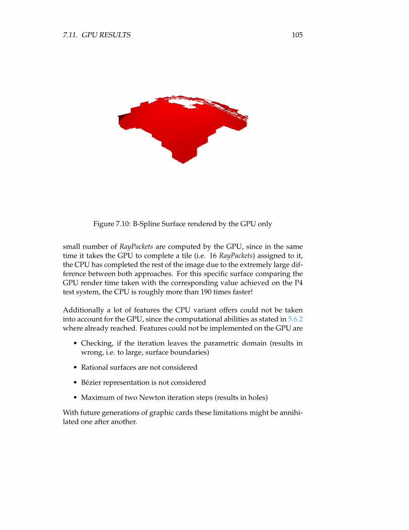
7.11. GPU RESULTS 105
Figure 7.10: B-Spline Surface rendered by the GPU only
small number of RayPackets are computed by the GPU, since in the sametime it takes the GPU to complete a tile (i.e. 16 RayPackets) assigned to it,the CPU has completed the rest of the image due to the extremely large dif-ference between both approaches. For this specific surface comparing theGPU render time taken with the corresponding value achieved on the P4test system, the CPU is roughly more than 190 times faster!
Additionally a lot of features the CPU variant offers could not be takeninto account for the GPU, since the computational abilities as stated in 5.6.2where already reached. Features could not be implemented on the GPU are
• Checking, if the iteration leaves the parametric domain (results inwrong, i.e. to large, surface boundaries)
• Rational surfaces are not considered
• Bézier representation is not considered
• Maximum of two Newton iteration steps (results in holes)
With future generations of graphic cards these limitations might be annihi-lated one after another.

106 CHAPTER 7. RESULTS

Chapter 8
Conclusions & Future Work
In this work it was shown, that it is possible and worthwhile to use NURBSsurfaces as the geometric primitive for interactive ray tracing on singlecommodity PCs. Compared to the common triangle ray tracer, frame ratesare naturally not as high. Nevertheless there are several advantages whenray tracing NURBS directly, including lower memory consumption, espe-cially for more sophisticated scenes, as well as artifact free rendering of ex-treme close up shots, without any additional effort. Furthermore, requiredpreprocessing time is reduced and artifacts, due to errors during tessella-tion of trimmed surfaces, are avoided.
It was also shown, that it is advisable to render low complex NURBS sur-faces with a reasonable number of control points and a basis function de-gree with less than seven. By exceeding these soft limits (depending onmodel scale and complexness) errors will occur in form of missed hits.This is due to the limited accuracy of single precision floating point val-ues. Using double precision is not a real solution, but relaxes this limi-tation slightly, however performance dramatically decreases, since this isnot compatible with SIMD execution yet. By using the baseline evaluationmethod any surface can be processed, regardless of control point grid reso-lution or degree, however frame rates are far from interactive in that case.
The additional usage of a GPU turned out not to be worthwhile yet. Theperformance achieved was slower by more than an order of magnitudecompared to CPU computation on even only mediocre processors. Themain problem is the complexity of the intersection test in contrast to therelatively limited computational abilities of recent GPUs. Problematic isthe maximum number of temporary registers as well as the number of ex-ecutions performed, which was effectively limiting the process to only oneor two Newton iteration steps, which is definitively not sufficient. On theone hand it might be possible to implement the algorithm by using a mul-
107

108 CHAPTER 8. CONCLUSIONS & FUTURE WORK
tipass approach, but on the other hand, this will slow down performanceeven further making it rather useless for interactive rendering. However,performance as well as the abilities of the instruction sets for graphic cardsare developing extremely fast, so it might be still interesting to keep an eyeon the development.
It turned out, that one of the biggest issues actually is the limited accu-racy of floats, when dealing with NURBS that have many control points ora high degree. Besides that, the frame rate goes down considerably withsuch kind of surfaces. Thus it would be worthwhile for future work to finda solution to both problems, especially because often real life data sets con-tain geometries that are not represented in an optimal manner. A possibleand very promising approach would be to integrate another step into thepreprocessing pipeline, where large and/or high degree surfaces will besplit up into several less difficult patches, i.e. each with only a small num-ber of control points and a basis function degree of preferably three or five.For these patches the accuracy will be sufficient and performance will re-main good.
Additionally it might be interesting to re-integrate the work from [12] intocrianusurt by adding support for triangles from the original ray tracer dream.Currently even flat surfaces like walls and floors have to be constructedby using NURBS, which is of course not optimal as for flat surfaces trian-gles are well suited. By combining triangle/Bézier/NURBS functionality itwould be possible to employ some kind of level of detail hierarchy, wherepatches close to the viewer are rendered using the NURBS representation,in middle distance the Bézier representation is used and in the far distanceonly the control net is rendered using triangles for example.
Last but not least, a very promising development is the upcoming Cell-Processor, a specialized chip for vector operation designed by IBM andToshiba. This chip will be first seen in Sonys new Playstation 3, but it willhopefully also be available by other means. A single Cell processor featuresone POWER based processor element (PPE) and eight Synergistic ProcessorElements (SPE), each of which is capable of full SIMD operation on 128 bitregisters. Basically this sums up to eight SIMD units for parallel use. To-gether these will reach a performance peak of 256 GFLOPS for single floatprecision operation. Considering that crianusurt is perfectly designed forthis kind of execution, it would be very interesting and promising to portit to the CELL architecture1, when available.
1Even if the CELL will not be available for PCs, it still might be possible to port crianusurtto the Playstation 3 itself, as a linux kit is expected to be realeased for it, just the same wayit was for the predecessor

Appendix A
libNURBSIntersectionKernelCommands Overview
In the following the API of the NURBSIntersectionKernel is explained. Somefunctions are only applicable to either NURBS or Bézier, in that case thesemethods have a leading [N] or [B] before their header. Those that have notare useable for both free form surface types
A.1 Acquiring an Instance
static NURBSIntersectionKernel* Instance(int ID);
param ID: has to be between 0 and MAX_NUMBER_OF_THREADS (de-fault:8)return: An instance of the kernel that can be used by one thread
A.2 Kernel Configuration
void cfgIndex(const int index);
param index: the unique index of the surface the kernel will be configuredfor
void cfgActiveComponents(bool4* const active);
param active: Specifies active components. Computation will be executedfor every element that is true. If all are false no computation will be per-formed at all
109

110APPENDIX A. LIBNURBSINTERSECTIONKERNELCOMMANDS OVERVIEW
[N] void cfgBasicDataVector(float4* const basicData);
param basicData: sets the basic data for the NURBS patch.Format: (Number of control points in U direction, number of control pointsin V direction, basis function degree in U direction, basis function degreein V direction)
void cfgBoxMinMaxUV(float4* const minU, float4* const maxU, float4*const minV, float4* const maxV);
param minU: minimum u parameter value for this current intersection test.This value is provided by the last bounding box that was hit, i.e. local validparametric domainFormat: (minU, minU, minU, minU)param others analog to minU
[N] void cfgSurfaceMinMaxUV(float4* const minMaxUV);
param minMaxUV: minimum and maximum u/v parametric values for thesurface being tests, i.e. global valid parametric domainFormat: (minimum U, maximum U, minimum V, maximum V)
void cfgControlPoints(float4* const controlPoints);
pram controlPoints: the control points for this surfaceFormat: (x1, y1, z1, w1), . . . , (xn, yn, zn, wn)
[N] void cfgBasisFunctions(float4* const basisFunctions);
param basisFunctions: each basis function is represented by a number offloat4 variables according the value of PIXELPERFUNCTION which is setin NURBSIntersectionKernel.h. First all basis function in u direction arestored after which the function in v direction follow. For each parametricdirection all intervals are stored in an ascending order, where each intervalstores a number of basic functions equalling the order of the basis function,also in ascending order according to the i loop value of the sum. Refer to3.5.1 or figure 3.15 for a more detailed discussion.
[N] void cfgKnotVectors(float4* const knotVectors);
param knotVectors: stores both knot vectors. Knot vector values in u direc-tion are stored in the first components, respectively v knot vector values arestored in the second components of each float4 variable. Third and fourthcomponents are not being used. Refer to 3.5.1

A.3. GLOBAL KERNEL CONFIGURATION 111
[N] void cfgBFOfsset(float4* const offset);
param offset: the number of basis functions in u parametric direction, i.e. theoffset to the first basis function in v direction
cfgTrimmingCurves(vector<BezierCurve*>* const curves);
param curves: all trimming curve segments for this surfaces stored in a STLvector in no particular order
void cfgRays(PrimaryRays const* rays);
param rays: to be set if the intersection test shall be computed with a packetof primary rays, i.e. rays having an identical origin
void cfgRays(ShadowRays const* rays);
param rays: to be set, if a shadow test shall be performed
void cfgRays(SecondaryRays const* rays);
param rays: to be set if a intersection with a packet of secondary rays shallbe computed, i.e. rays with different origins
A.3 Global Kernel Configuration
void cfgMaxNewtonStep(const int maxNS);
param maxNS: the maximum number of newton steps that will be per-formed, before the intersection test will be interrupted. Default:6
[N] void cfgPixelPerFunction(const int ppf);
param ppf : the number of float4 variables that will be used to store one basisfunction. Maximum degree of a function: ppf*4-2. Default:2
void cfgNewtonEpsilon(const float4& eps);
param eps: the epsilon value that defines the maximum distance to the realroot that will still be regarded as an intersection. Values closer to 0 willyield more exact results but more likely missed hits. Default:0.001

112APPENDIX A. LIBNURBSINTERSECTIONKERNELCOMMANDS OVERVIEW
A.4 Evaluations and Intersections
void intersect(HitPacket& hits, bool doTrimming, bool doBezier = false);
The previously configured surface data will be used to perform an inter-section test with a primary ray packetparam hits: stores the results of the intersection testparam doTrimming: if true, trimming test will be performedparam doBezier: use high performance Bézier intersection test
void intersect(bool4& mask, float4& scale, bool doTrimming);
The previously configured surface data will be used to perform a shadowtest with a shadow ray packetparam mask: Stores the result of the test with false indicating a shadowedpixel. If components were set to false before calling this method they willalways stay false, i.e. the shadow test will not be performed on these com-ponentsparam scale: Currently not used in this implementation. Is planned to beused for computing transparencies param doTrimming: if true, trimming testwill be performed
void intersectSecondary(HitPacket& hit, bool doTrimming);
Performs an intersection test with secondary rays (reflected rays for exam-ple) Note: Secondary reys for Bézier surfaces not supported yetparam hit: stores the results of the intersection testparam doTrimming: if true, trimming test will be performed
[N] void evaluate(const float4& u, const float4& v, const bool derivativeU,const bool derivativeV, float4& resX, float4& resY, float4& resZ) const;
Evaluates the NURBS surface at given u and v parameterparam u: four u parameter valuesparam v: four v parameter valuesderivativeU: if true, partial derivative u will be computedderivativeV: if true, partial derivative v will be computedresX: stores the four x values of the resulting pointsresY: stores the four y values of the resulting pointsresZ: stores the four z values of the resulting points

A.4. EVALUATIONS AND INTERSECTIONS 113
[B] void evaluateBS(float4 &u, float4 &v, float4 &resX, float4 &resY, float4&resZ) const;
Evaluates the Bézier surface at given u and v parameterparam u: four u parameter valuesparam v: four v parameter valuesresX: stores the four x values of the resulting pointsresY: stores the four y values of the resulting pointsresZ: stores the four z values of the resulting points
[B] void evaluateBSDerivativeU(const float4 &u,const float4 &v, float4&resX, float4 &resY, float4 &resZ) const;
Evaluates the partial derivative u of the Bézier surface at given u and vparameterparam u: four u parameter valuesparam v: four v parameter valuesresX: stores the four x values of the resulting pointsresY: stores the four y values of the resulting pointsresZ: stores the four z values of the resulting points
[B] void evaluateBSDerivativeV(const float4 &u,const float4 &v, float4&resX, float4 &resY, float4 &resZ) const;
Evaluates the partial derivative v of the Bézier surface at given u and vparameterparam u: four u parameter valuesparam v: four v parameter valuesresX: stores the four x values of the resulting pointsresY: stores the four y values of the resulting pointsresZ: stores the four z values of the resulting points
void evaluateNormal(const float4& u, const float4& v, VectorPacket& nor-mals, bool doBezier = false) const;
evaluates the normal at the given parameter values u and vparam u: four u parameter valuesparam v: four v parameter valuesnormals: vector packet soring the four resulting normalsdoBezier: if true, use high performance Bezier mode
trimmed(const float4 &u, const float4 &v, bool4 &mask) const;
performes a trimming test on current surface on given u and v parametervalues

114APPENDIX A. LIBNURBSINTERSECTIONKERNELCOMMANDS OVERVIEW
param u: four u parameter valuesparam v: four v parameter valuesmask: every value that is false denotes a trimmed point

Bibliography
[1] Oliver Abert. Interaktives raytracing von getrimmten bikubischenbézier flächen unter verwendung von simd instruktionen, December2004. 1, 2, 36, 65, 74, 97
[2] Alias maya,http://www.alias.com. 28
[3] Robert Bärz. Paralleslisierung von ray tracing berechnungen in einemheterogenen netzwerk, October 2004. 24
[4] Phong Bui-Tuong. Illumination for computer genereated pictures. InCommunications of the ACM, volume 18(6), pages 311–317, June 1975.22
[5] Philipp Slusallek Carsten Benthin, Ingo Wald. Interactive ray tracingof free-form surfaces. In ACM AFRIGRAPH, pages 99–106, 2004. 1
[6] de casteljau’s algorithm,http://en.wikipedia.org/wiki/de_casteljau’s_algorithm, September2005. 78
[7] M.G. Cox. The numerical evaluation of b-splines. In Journal of Institu-tional Mathematical Application, volume 10, pages 134–149, 1972. 7
[8] C. de Boor. on calculating with b-splines. In journal of ApproximationTheory 6, pages 50–62, 1972. 7
[9] Microsoft directx,http://www.microsoft.com/windows/directx/default.aspx. 17
[10] T.F. Riesenfeld E. Cohen, T. Lyche. Discrete b-splines and subdivi-sion techniques in computer aided geometric design and computergraphics. In Computer Grahpics and Image Processing, volume 14, pages87–111, 1980. 13
[11] James Clark Edwin Catmull. Recursevely generated b-spline surfaceson arbitrary topological meshes. In Computer-Aided Design, volume10(6), pages 350–355, September 1978. 65
115

116 BIBLIOGRAPHY
[12] Markus Geimer. Interactive ray tracing, August 2005. 30, 55, 63, 64,108
[13] Andrew S. Glassner. Space subdivision for fast ray tracing. IEEE Com-puter Graphics and Applications, 4(10):15–22, 1984. 28
[14] Andrew S. Glassner. Spacetime ray tracing for animation. IEEE Com-puter Graphics and Applications, 8(2):60–70, 1988. 28
[15] Hyper threading technology,http://www.intel.com/technology/hyperthread. 101
[16] Intel corp. ia-32 architecture software developers manual. 2004. 2
[17] Frederik W. Jansen. Data structures for ray tracing. Data structures forraster graphics, pages 57–73, 1986. 28
[18] John Salmon Jeffrey Goldsmith. Automatic creation of object hierar-chies for ray tracing. In IEEE Computer Graphics and Applications, vol-ume 7, pages 12–20, May 1987. 30
[19] Henrik Wann Jensen. Realistic image Synthesis Using Photon Mapping.2001. 30
[20] Henrik Wann Jensen. State of the art in monte carlo ray tracing forrealistic image synthesis. In SIGGRAPH 2001 Course Notes CD-ROM.ACM SIGGRAPH, 2001. 22
[21] James T. Kajiya. Ray tracing parametric surfaces. In Computer graphics,volume 16(3), pages 245–254. ACM SIGGRAPH, July 1982. 64
[22] Andreas Langs. Photon mapping unter verwendung eines simd raytracers, June 2005. 30
[23] Charles T. Loop. Smooth subdivision surfaces based on triangles. InMaster’s thesis, University of Utah, 1987. 65
[24] William R. Mark, R. Steven Glanville, Kurt Akeley, and Mark. J Kil-gard. Cg: a system for programming graphics hardware in a c-likelanguage. ACM Transactions on Graphics (TOG), 22(3):896–907, 2003.17
[25] Oliver Abert Markus Geimer. Interactive ray tracing of trimmed bicu-bic bézier surfaces without triangulation. In WSCG’2005, 2005. 1
[26] William Martin, Elaine Cohen, Russell Fish, and Peter Shirley. Practi-cal ray tracing of trimmed NURBS surfaces. Journal of Graphics Tools:JGT, 5(1):27–52, 2000. 66, 67

BIBLIOGRAPHY 117
[27] Richard Bartels Michael Sweeney. Ray tracing free-form b-spline sur-faces. In IEEE Computer Graphics and Applications, volume 6(2), pages41–49, February 1986. 66
[28] Motorola, inc. altivec technology programming interface manual,1999. 2
[29] Newton’s iteration,http://mathworld.wolfram.com/newtonsiteration.html. 65
[30] Opengl shading language,http://www.opengl.org/documentation/oglsl.html. 18
[31] Openrt,http://www.openrt.de. 27
[32] Changway Wang Peter Shirley. Direct lighting calculation by montecarlo integration. In Proceedings of the second Eurographics Workshop onRendering, june 1991. 22
[33] H. Prautzsch. A short proof of the oslo algorithm. In Computer AidedGeometry Design, volume 1, pages 95–96, 1984. 13
[34] David F. Rogers. An Introduction to NURBS with Historical Perspective.Morgan Kaufmann Publishers, 2000. 5, 82, 94
[35] Peter Shirley. Realistic Ray Tracing. 21
[36] Ruei-Chuan Chang Shyue-Wu Wang, Zeng-Chung Shih. An efficientand stable ray tracing algorithm for parametric surfaces. Journal ofInformation Science and Engeneering, 18:541–561, 2001. 66
[37] ANSI/IEEE standard 754-1985. Ieee standard for binary floating-pointarithmetic, 1985. 82
[38] R. Séroul. programming for Mathematicians, chapter 10.6 Evaluation ofPolynomials: Horner’s Method, pages 216–262. Springer Verlag, 2000.42
[39] Masanori Kakimoto Tomoyuki Nishita, Thomas W. Sederberg. Raytracing trimmed rational surface patches. In Computer Graphics, vol-ume 24(4), pages 337–345, August 1990. 75, 77
[40] H. Prautzsch W.Boehm. The insertion algorithm. In CAD, volume 17,pages 58–59, 1985. 13