Incentive Pass-through forResidential Solar Systems in California

1University of Texas at Austin; 2Lawrence Berkeley National Laboratory

C.G. Dong1, Ryan Wiser2, Varun Rai1

Abstract ........................................................................................................................ 1

1. Introduction ............................................................................................................. 1

2. Literature Review .................................................................................................... 4

3. Methods and Data ................................................................................................... 8

3.1 Structural Modeling ............................................................................................. 83.2 Reduced-form Regression .................................................................................... 123.3 Data ................................................................................................................... 12

4. Results .................................................................................................................... 18

4.1 Structural Modeling ............................................................................................. 184.2 Reduced-form Approach ....................................................................................... 23

5. Conclusions ............................................................................................................. 26

References .................................................................................................................... 28

Contents

Fig. 1. CSI EPBB Capacity Steps and Rebate Levels ..................................................... 3

Fig. 2. Equilibrium Depiction of Incentive Pass-through ............................................... 6

Fig. 3. California Residential PV System Trends: Average System Installation Price, Module Price and Monthly Installation ......................................................................... 14

Fig. 4. PG&E CSI Data: Residential Pre-rebate Installation Price, Rebate, and Cumulative Capacity ..................................................................................................... 15

Fig. 5. Pass-through Rates for 49 California Counties: Structural-Modeling Approach ...................................................................................................................... 22

Fig. 6. System-level Regression Results for County-specific Pass-through Rates ........ 25

Table 1. County-level Summary Statistics for Structural Modeling: 2001–2012 ........... 16

Table 2. System-level Summary Statistics for the Reduced-form Regression Analysis: 2001–2012 .................................................................................................... 17

Table 3. Regression Output: PV Demand and Supply Relation for San Diego County and All Counties ............................................................................................................ 21

Table 4. System-level Regression Results for 49 California Counties Together ............. 24

List of Figures and Tables

Abstract The deployment of solar photovoltaic (PV) systems has grown rapidly over the last decade, partly because of various government incentives. In the United States, among the largest and longest-running incentives have been those established in California. Building on past research, this report addresses the still-unanswered question: to what degree have the direct PV incentives in California been passed through from installers to consumers? This report helps address this question by carefully examining the residential PV market in California (excluding a certain class of third-party-owned PV systems) and applying both a structural-modeling approach and a reduced-form regression analysis to estimate the incentive pass-through rate. The results suggest an average pass-through rate of direct incentives of nearly 100%, though with regional differences among California counties. While these results could have multiple explanations, they suggest a relatively competitive market and well-functioning subsidy program. Further analysis is required to determine whether similar results broadly apply to other states, to other customer segments, to all third-party-owned PV systems, or to all forms of financial incentives for solar (considering not only direct state subsidies, but also utility electric bill savings and federal tax incentives).

1 Introduction The deployment of solar photovoltaic (PV) systems has grown rapidly over the last decade. While global annual installed PV capacity was less than 0.3 gigawatts (GW) in 2000, this number surpassed 38 GW in 2013 (EPIA, 2014). Deployment in the United States has also grown rapidly, from around 0.004 GW of newly installed capacity in 2000 to more than 4 GW in 2013 (Sherwood, 2013; SEIA/GTM, 2014). A key driving force behind such growth has been the myriad of government incentive programs promoting solar deployment, often motivated by a desire to address two possible market failures indirectly: the unpriced environmental consequences of conventional energy sources (Bezdek, 1993; Painuly, 2002) and learning-by-doing and innovation spillover effects in the PV industry (McDonald and Schrattenholzer, 2001; van Benthem et al., 2008). Other factors driving policy decisions to support solar include the potential benefits of energy resource diversity and the possibility of new jobs and economic activity in the solar sector.1

Many federal and state programs in the United States offer financial incentives (often in the form of up-front rebates) to remove capital barriers for customers to adopt PV. With a budget of more than $2 billion and a program life of a decade (2007–2016), the California Solar Initiative (CSI) is a good example of a large-scale U.S. program. The major aim of the CSI is to spur solar

1 Many economists would question whether direct support for the solar sector is the most efficient mechanism for correcting market failures, and they would also question whether some of the policy motivations listed here even call for government intervention (e.g., jobs and economic activity).

1

deployment, with a goal of 1.94 GW of new solar capacity by 2016 (CPUC, 2014). However, the degree to which the financial incentives offered by the CSI have passed through to PV customers has not been studied systematically. In practice, though PV customers could apply for the incentives directly, the vast majority instead authorizes PV installers to submit incentive claims on their behalf; PV installers then provide PV customers a discount on the installation prices that is nominally equal to the incentive received. Whether delivered as a discount via installers or directly to customers, however, it is unclear if incentives are fully passed through to customers, because installers may opt to adjust their pre-incentive PV prices to account for those incentives. The pass-through rate, therefore, crucially depends on how PV installers determine pre-incentive PV prices. If PV installers price their systems on a pre-incentive basis higher when incentives are larger, then PV customers will not benefit fully from the provision of the incentives, and instead installers will retain some fraction of the available incentive. This especially might be the case if PV installers face high customer demand for PV and low demand elasticity.

This report focuses on the incentive pass-through question for the CSI while also using data from the previous residential incentive program in California—the Emerging Renewables Program (ERP)—because these two programs are collectively the largest and longest-running state-level PV incentive programs in the United States. Previous studies that have used California’s solar installation data to conduct various types of econometric analyses include Bollinger and Gillingham (2012), Burr (2012), Henwood (2014), Hughes and Podolefsky (2013), and van Benthem et al. (2008). Our work leverages the sizable dataset of system-level PV prices managed by Lawrence Berkeley National Laboratory (LBNL), and is part of a larger body of research conducted by LBNL, Yale University, University of Wisconsin, and University of Texas at Austin that is exploring, more broadly, the drivers of PV price variability in the United States. Our focus here is on residential PV systems in California, and we exclude “appraised value” third-party-owned (TPO) PV systems; as such, the pass-through rates estimated here do not apply outside of California or to appraised-value TPO systems. Moreover, the results presented here focus narrowly on the pass-through rate for direct solar incentives offered by the CSI and ERP. We do not evaluate value-based pricing more broadly, considering the combined impact of direct state incentives, electric utility bill savings, and federal tax incentives.

At the beginning of the CSI in early 2007, a typical residential PV system could receive an upfront rebate of $2.5/W based on system size (and scaled by the expected performance of the system), whereas the system installation price was on average around $10/W.2 Within each of the three largest electric utility service territories in California, the rebate level then decreased stepwise once a certain capacity goal for each step had been achieved. The CSI established nine steps for the whole process, with the final rebate level at $0.2/W, after which the program ends. Fig. 1 shows these nine steps, from Step 2 to 10, for the major incentive type available to the

2 Prior to the CSI, the ERP at times offered even higher rebate levels.

2

residential sector: Expected Performance Based Buydown (EPBB).3 For each step, the CSI established a capacity goal and a corresponding rebate level. The steps move to the next level once the stepwise capacity goal is achieved. The three largest investor-owned utilities (IOUs) in California administer this rebate program in their own territories with different capacity goals, and they have generally moved at different paces along the rebate ladders. Information on the then-current rebate level and the remaining capacity goals before the step changes has been constantly updated at csi-trigger.com for each IOU and by customer sector.

The nine step changes (also called “step downs”) provide sufficient variation of rebates over time and between utilities to study the question of incentive pass-through (also called “subsidy pass-through” or “subsidy incidence”), i.e., how much of the incentive has been passed through to PV consumers. This concept of incentive pass-through is analogous to that of tax pass-through (also called “tax incidence”), where the question is whether consumers or suppliers bear a tax burden, and has been used in a wide variety of other contexts. Early work on tax incidence includes Due (1954), Brownlee and Perry (1967), and Woodard and Siegelman (1967); Section 2 discusses additional literature in this area. Pass-through rates have been commonly evaluated either through structural modeling or reduced-form regression analysis, and we use both methods in the present study. Regression discontinuity (RD) designs (a special form of reduced-form regression analysis) have also often been employed to evaluate pass-through rates; though we do not implement such designs in the present report, a companion report to be published in the near

3 The other type is the Performance-Based Incentive (PBI), which accounts for less than 0.5% of the residential systems; the present study only covers EPBB.

Fig. 1. CSI EPBB Capacity Steps and Rebate Levels

3

future uses RD analysis and includes pass-through estimates that are similar to those presented in the current report.

Though the CSI has now wound down as final solar capacity targets have been reached, estimating the historical pass-through rate has important broader implications for solar policy design. The question of the relative distribution of incentives to PV customers and PV installers should be an important aspect of the CSI policy evaluation, especially as policymakers would presumably prefer that solar incentives are largely passed through to the intended recipients: PV customers. Moreover, incentive programs of various types still exist in the U.S. and other countries; thus, the historical performance of the CSI is relevant not only as an ex-post analysis in California, but potentially has broader policy implications for other solar incentive programs both nationally and internationally. Understanding the pass-through rate also illuminates the level of competition in local solar markets and, therefore, may help guide solar deployment policy efforts. In particular, if the pass-through rate is found to be low (i.e., a large portion of the incentive is absorbed by installers), this may signal to policymakers the need to focus more of their efforts on lowering entry barriers and increasing competition among installers. On the other hand, a high pass-through rate might be an indication of a well-functioning incentive program.

The rest of the report is organized as follows. In Section 2, we summarize the pass-through literature, including both theoretical and empirical work. Section 3 discusses our methods and underlying data. In Section 4, we show our main results for the CSI/ERP incentive pass-through rate estimation, and we compare the pass-through rates estimated by structural modeling and by reduced-form regression. We conclude the report in Section 5.

2 Literature Review Similar to tax pass-through, the incentive pass-through rate (𝑃𝑇) can be formally defined as:

𝑃𝑇 = − 𝑑(𝑁𝑒𝑡 𝑃𝑟𝑖𝑐𝑒)𝑑(𝐼𝑛𝑐𝑒𝑛𝑡𝑖𝑣𝑒) × 100% (1)

i.e., the (absolute) marginal impact of incentive changes on the net (post-incentive) price paid by consumers. A pass-through rate of 100% implies that incentives are fully passed through to customers, whereas a rate of less than 100% means that some portion of the incentives is retained by the PV installer.

Sometimes, researchers instead study variations in pre-incentive prices (not net, post-incentive prices); in this case, the pass-through rate can still be derived from the results, since:

𝑃𝑇 = −𝑑(𝑃𝑟𝑖𝑐𝑒−𝐼𝑛𝑐𝑒𝑛𝑡𝑖𝑣𝑒)𝑑(𝐼𝑛𝑐𝑒𝑛𝑡𝑖𝑣𝑒) × 100% = �1 − 𝑑(𝑃𝑟𝑖𝑐𝑒)

𝑑(𝐼𝑛𝑐𝑒𝑛𝑡𝑖𝑣𝑒)� × 100% (2)

In other words, the pass-through rate in this instance is 1 minus the coefficient on the incentive term (in the regression of pre-incentive prices), which is then multiplied by 100%.

4

In public economics theory, researchers have derived the pass-through rate based on the curvature of demand and production cost curves as well as the level of market competition (Delipalla and Keen, 1992; Fullerton and Metcalf, 2002; Sijm et al., 2012; Stern, 1987; Vivid Economics, 2007). Essentially, pass-through is a market-equilibrium concept. In the case of PV incentives, those incentives may act as a positive demand shifter (increasing demand for PV), but they might also impact PV costs depending on the shape of the marginal cost curve. In addition to demand and production cost curvature, the level of market competition also plays a key role in determining the pass-through rate.

Since pass-through is an equilibrium concept, it becomes necessary to estimate demand, supply, and equilibrium conditions simultaneously. Fig. 2 provides a simple illustration of the incentive pass-through concept. With a linear supply curve (or marginal cost function) and a linear demand curve in two periods, the pass-through rate is equal to the absolute change in net price paid by consumers (∆𝑁𝑃) divided by the incentive level change (𝑅). In a more-flexible (and not necessarily linear) supply and demand framework, this is the same as taking the first derivative of net price with respect to the incentive (Eq. 1). This line of argument ties closely to assessing market power using the elasticity-adjusted Lerner index,4 also called the “conduct” or “market power” parameter (Genesove and Mullin, 1998; Wolfram, 1999).5 Furthermore, estimating pass-through rates has strong implications for various welfare analyses and market-design problems (Weyl and Fabinger, 2013).

4 The Lerner index describes a firm’s market power, measured by (price – marginal cost) / price. The index ranges from 0 to 1, i.e., the percentage of the firm’s mark-up to the price. 5 The conduct parameter approach was previously known as the conjecture variation approach, which was not without debates in the literature. While there are several outstanding critiques of this approach (Corts, 1999; Reiss and Wolak, 2007), other literature tends to justify its evolutionary consistency (Dixon and Somma, 2003; Possajennikov, 2009; Rachapalli and Kulshreshtha, 2013). Based on Jaffe and Weyl (2013), there was a recent resurgence in studies using this approach, both theoretical and empirical (see references cited there).

5

Fig. 2. Equilibrium Depiction of Incentive Pass-through

Note: The introduced incentive level R in period 2 moves the demand curve from D1 to D2, and a new market equilibrium emerges at (P2*, Q2*) assuming the supply curve remains the same: S1 = S2. The net price paid by

consumers in period 1 is the market price P1*, while in period 2 it is (P2* - R), so the absolute net price change is ΔNP. Though this logic applies to an increase in incentive levels, the order of time can be reversed to create a

similar case for incentive-level reductions.

Empirically, there are two ways to estimate the pass-through rate. The first is to estimate the pass-through rate through structural modeling, where researchers impose theoretical assumptions on the demand function, production technology, and how suppliers maximize profits responding to others’ change in market behaviors. Genesove and Mullin (1998) applied this method with various functional forms for demand to the refined sugar industry and verified it with reliable marginal cost data. Barnett et al. (1995) used a translog functional form for the production cost and compared cigarette tax incidence between the federal level and the state level. Other similar work includes Besley and Rosen (1999), Bettendorf and Verboven (2000), Clay and Troesken (2003), and Karp and Perloff (1989), among others. Somewhat differently, Bergin and Feenstra (2009) derived the pass-through rate in a monopolistic competition framework. Further, Kim and Cotterill (2008) used a discrete choice demand model (following Berry et al., 1995) for processed cheese and estimated pass-through rates for input-cost changes. To date, no structural-modeling work has been done for solar incentive pass-through.

The second method for estimating pass-through is by employing a reduced-form regression analysis to estimate the marginal impact of a tax (or incentive) on consumer prices. Researchers have applied this method to study the pass-through question for various taxes (Besley and Rosen, 1999; Carbonnier, 2007; Marion and Muehlegger, 2011; Poterba, 1996), exchange rates (Choudhri and Hakura, 2012; Gopinath et al., 2010; Marazzi et al., 2005), and upstream cost shocks (Alexeeva-Talebi, 2011; Gron and Swenson, 2000; Vavra and Goodwin, 2005). Several

Pass-through = ΔNP / R * 100%

6

studies have also looked at incentive pass-through specifically, focusing on, for example, federal tax credits for the Toyota Prius (Sallee, 2011), agricultural subsidies to farmland (Kirwan, 2009; Hendricks et al., 2012), and automobile manufacturer promotions (Busse et al., 2006). Though difference-in-difference and fixed-effects models are typically used in these regression analyses, few make the explicit connection between this work and the pass-through theory in public economics.

As for solar incentives, a few studies have looked at the pass-through question with reduced-form regression analysis. Several unpublished works have studied the question using CSI data (Henwood, 2014; Peterman, 2012; Podolefsky, 2013). Podolefsky (2013) found a low incentive pass-through rate of 17% (83% enjoyed by firms) but only looked at the pass-through for the federal solar Investment Tax Credit (ITC), not for the CSI incentives. Henwood’s (2014) best estimate6 stated that only 36% of the CSI rebate was enjoyed by consumers (64% enjoyed by firms). Neither social demographics nor many PV system characteristics were controlled for in the analysis, however, and these omitted variables could confound the pass-through relationship if they are not equally distributed before and after the rebate-level changes. Wiser et al. (2007) estimated the impact of rebate levels on pre-rebate installed prices under an earlier PV rebate program in California, finding a coefficient of 0.56–0.73. Based on Eq. (2), the corresponding pass-through rate was 27%–44%. No time fixed effects (other than a linear monthly trend variable) were included to control for the seemingly positive correlation between rebate and price; additionally, because the work is somewhat dated, its results might not hold in the evolving solar market of today. Shrimali and Jenner (2013), meanwhile, studied 27 PV subsidy programs in 16 U.S. states over the period 1998–2009 and found that cash incentives were correlated with lower PV balance-of-system (BOS) costs (i.e., system price minus module cost). Similarly, Davidson and Steinberg (2014) claim that the decreasing CSI incentive drove down reported installation prices; however, PV incentives and prices could be automatically positively correlated, since they both decreased over time, and the causality could go in the other direction.

This report contributes to the broad pass-through literature by focusing on the largest state-level solar incentive programs in the United States: the CSI and, previously, the ERP. Our methods include both structural modeling and reduced-form regression analysis. We consider these two approaches to be complementary (Timmins and Schlenker, 2009). While the structural-modeling approach can better capture the equilibrium relationship and produce useful market competition results, the reduced-form analysis requires fewer structural assumptions and allows for more-flexible functional forms.7 The combination of both approaches provides a test for the robustness of the pass-through results. Finally, as indicated earlier, in a companion paper we also use RD designs to take advantage of PV incentive step-down opportunities and geographic

6 Henwood (2014) also tried other model specifications, but the results were unstable. 7 The reduced-form analysis could potentially suffer from specification errors and omitted cost components bias, which can be avoided by assuming a constant pass-through rate. See MacKay et al. (2014) for more details.

7

discontinuities in incentive levels between utilities. The current report complements those to-be-published RD results in terms of external validity.

3 Methods and Data As mentioned above, we use both structural modeling and reduced-form regression analysis to estimate the pass-through rate for the CSI and the ERP. Because of its greater complexity, we focus in Section 3.1 on explaining the structural-modeling framework. In Section 3.2, we briefly discuss the regression specification for the reduced-form approach. Section 3.3 then summarizes the data used to conduct our analyses.

3.1 Structural Modeling

The structural approach follows the established line of previous pass-through literature (Delipalla and Keen, 1992; Stern, 1987; Wolfram, 1999) and estimates a PV demand function, a supply relation, and the conduct parameter simultaneously. The pass-through rate can then be calculated from the parameters obtained through a predefined formula, together with appropriate confidence intervals.

Assume market-level PV demand as:

𝑄 = 𝑄(𝑃,𝑋) (3)

where 𝑃 is the pre-incentive system installation price8 ($/W) and 𝑋 is a vector of other control variables. Each installer 𝑖 in the market is assumed to face the same demand and maximizes its own profits:

max{𝑞𝑖} 𝜋𝑖 = �𝑃� + 𝑠�𝑞𝑖 − 𝐶(𝑞𝑖,𝑍) (4)

where 𝑃� is the post-incentive price term (i.e., net price), 𝑠 is the incentive (or subsidy) level ($/W), 𝑞𝑖 is the quantity produced by this installer, and 𝐶 is the production cost, as a function of quantity and other factors 𝑍.

Assuming installers compete in quantity, the first order condition of Eq. (4) is:

𝑃� + 𝑠 + 𝜃𝑃𝑄𝑞𝑖 = 𝐶𝑞 (5)

where 𝜃 = 𝜕𝑄𝜕𝑞𝑖

is the conduct (or market power) parameter that captures the responses of all firms

when one installer changes its quantity.9 The parameter 𝜃 nests various forms of imperfect

8 Theoretically, the post-incentive system price (i.e., net price) should be used in the demand equation, since that is the price that PV consumers face. However, in our case, this is less important because the demand slope coefficients associated with either the price term or the net price term are almost the same, i.e., the incentive variable is roughly exogenous to the relationship between price and demand quantity. In addition, using the net price term creates a weak instrument problem if we use PV hardware cost as a supply shifter to instrument it, because the correlation between net price and PV hardware cost is very small. On the other hand, PV hardware cost is highly correlated with pre-incentive system prices, making it a very useful instrumental variable for the price term in the demand equation.

8

competition (Weyl and Fabinger, 2013): 𝜃 = 𝑁 refers to monopoly or tacit collusion with 𝑁 as the number of installers in the market, 𝜃 = 0 refers to perfect or Bertrand competition, and 𝜃 = 1 refers to Cournot competition. Furthermore, 𝑃𝑄 and 𝐶𝑞 are first derivatives of system price and product cost with respect to different quantity terms.

A market-level average of Eq. (5) can be derived as:

𝑃� + 𝑠 + 𝜃∗𝑃𝑄𝑄 = 𝐶𝑄 = 𝑀𝐶(𝑄,𝑍) (6)

where 𝜃∗ = 𝜃𝑁

, and 𝐶𝑄 and 𝑀𝐶(𝑄,𝑍) are the market-level marginal cost.10 The values of 𝜃∗ being equal to 1, 0, and 1/𝑁 correspond to monopoly, Bertrand competition, and Cournot competition, respectively; this is why 1/𝜃∗ is usually interpreted as the “equivalent number of firms” in the literature.

With this setup, we can then derive the incentive pass-through rate by taking the derivative of 𝑃� with respect to 𝑠 from Eq. (6). Following Delipalla and Keen (1992), the pass-through rate formula is as follows:

−𝑑𝑃�

𝑑𝑠= 1

1+𝜃∗(1+𝐴+𝐸) (7)

where

𝐴 = − 𝐶𝑄𝑄𝜃∗𝑁∙𝑃𝑄

and 𝐸 = −𝑃𝑄𝑄𝑄𝑃𝑄

(8)

In other words, 𝐴 is the relative slope of marginal costs to inverse demand (𝐶𝑄𝑄/𝑃𝑄) along with the market conduct parameter 𝜃∗ and the number of installers 𝑁 in the market. 𝐸 is the elasticity of the slope of inverse demand.

Following Wolfram (1999), Eq. (6) can be rewritten as the following supply-relation equation:

𝑃 = 𝑃� + 𝑠 = 𝑀𝐶(𝑄,𝑍) + 𝜃∗ 𝑃𝜂 (9)

or furthermore as:

𝜃∗ = 𝜂 ∙ 𝑃−𝑀𝐶(𝑄,𝑍)𝑃

(10)

where 𝜂 is the absolute price elasticity of PV demand evaluated at the pre-incentive price 𝑃, i.e., − 1

𝑃𝑄

𝑃𝑄

. That is why the conduct parameter 𝜃∗ is often called the elasticity-adjusted Lerner index.

The rest of the problem is then how to obtain estimates for parameters in Eq. (7): (𝜃∗,𝐴,𝐸).

9 Unlike Wolfram (1999), we do not differentiate 𝜃 by installers in order to make the notations simpler; the pass-through formulas are still the same. 10 This assumes 𝑞𝑖 enters the marginal cost function linearly for each firm, which is reasonable since the first two moments of quantity in the production cost function are presumably the dominant ones, i.e., there is less need to consider third or fourth power here.

9

To add a more-specific context to the above derivation, below we specify the functional forms for PV demand and marginal cost and then develop the corresponding supply-relation equation. According to Bresnahan (1982), the identification of the above structural model requires at least one exogenous demand shifter that not only moves the intercept up and down, but also changes the demand slope. Therefore, we include both a price term and an interaction term between the system price and another exogenous variable.

In particular, the PV demand function is specified as follows:

𝑄𝑡 = 𝛽0 + 𝛽1𝑄𝑡−1 + 𝛽2𝑃𝑡 + 𝛽3(𝑃 × 𝑆𝑢𝑚𝑚𝑒𝑟)𝑡 + 𝛽4(𝑆𝑢𝑚𝑚𝑒𝑟)𝑡 + 𝛽5(𝑇𝑃𝑂_𝑅𝑎𝑡𝑖𝑜)𝑡+ 𝛽6(#_𝑜𝑓_𝑍𝑖𝑝𝑐𝑜𝑑𝑒𝑠)𝑡 + 𝛽7(#_𝑜𝑓_𝐼𝑛𝑠𝑡𝑎𝑙𝑙𝑒𝑟𝑠)𝑡 + 𝛽8(𝐹𝑖𝑛_𝐶𝑟𝑖𝑠𝑖𝑠)𝑡 + 𝜀𝑑

= 𝛽2𝑃𝑡 + 𝛽3(𝑃 × 𝑆𝑢𝑚𝑚𝑒𝑟)𝑡 + 𝛽𝑋𝑡 + 𝜀𝑑 (11)

The measurement of all the variables is at the market level, which is defined here as each California county, following Davidson and Steinberg (2014). Time index 𝑡 refers to a calendar month. 𝑄𝑡 is then the monthly market demand of installed capacity (in kW), 𝑄𝑡−1 is market demand in the previous month and indirectly captures many critical local-demand influences (e.g., household income, demographics, etc.), and 𝑃 is pre-incentive installation price ($/W). The interaction term between 𝑃 and 𝑆𝑢𝑚𝑚𝑒𝑟 is to reflect that potential PV customers may respond to system price differently in different seasons,11 where we define 𝑆𝑢𝑚𝑚𝑒𝑟 as an indicator variable for the second and the third quarters of a year (April to September). 𝑇𝑃𝑂_𝑅𝑎𝑡𝑖𝑜 is the percentage of PV systems that are TPO, while #_𝑜𝑓_𝑍𝑖𝑝𝑐𝑜𝑑𝑒𝑠 and #_𝑜𝑓_𝐼𝑛𝑠𝑡𝑎𝑙𝑙𝑒𝑟𝑠 are the number of zip codes and installers at time t in the market (i.e., in the county). 𝐹𝑖𝑛_𝐶𝑟𝑖𝑠𝑖𝑠 denotes whether the system was installed in the financial crisis year of 2008. Lastly, 𝜀𝑑 is the error term. For the purpose of the remainder of this report and to simply the following equations, we further define 𝑋𝑡 as including all variables other than the two price terms.

Furthermore, we specify the market-level (in this case, county-level) average marginal cost as:

𝑀𝐶𝑡 = 𝛿0 + 𝛿1𝑄𝑡 + 𝛿2(𝐻𝑎𝑟𝑑𝑤𝑎𝑟𝑒𝐶𝑜𝑠𝑡)𝑡 + 𝛿3(𝐿𝑎𝑏𝑜𝑟𝐶𝑜𝑠𝑡)𝑡 + 𝜀𝑠 (12)

Eq. (12) can be considered the average of the installer-level marginal costs functions, since we only observe market-level hardware costs and labor costs. 𝐻𝑎𝑟𝑑𝑤𝑎𝑟𝑒𝐶𝑜𝑠𝑡 includes both module cost and inverter cost, and 𝐿𝑎𝑏𝑜𝑟𝐶𝑜𝑠𝑡 is based on the annual wages of three professions related to the BOS costs: roofer, electrician, and administrative (Ardani et al., 2012). Further, the average of installer-level marginal costs is assumed to depend on monthly county-level PV installations (𝑄𝑡), captured by 𝛿1.

According to Wolfram (1999), the supply-relation equation in Eq. (6) can be characterized as follows:12

11 As it turns out, it is important to include such an interaction term, as will become clearer in the discussion of model identification below. 12 Missing steps from Eq. (9) to Eq. (13) are (omitting the error term):

10

𝑃𝑡 = 11+𝜃∗

𝑀𝐶𝑡 + 𝜃∗

1+𝜃∗ℎ𝑡 + 𝜀𝑑� (13)

where ℎ𝑡 = 𝛽�𝑋𝑡−𝑄𝑃�

with �̂�𝑋𝑡 and 𝑄𝑝� defined in footnote 12. In other words, ℎ𝑡 is an imputed term

from the estimation of Eq. (11). We then plug in terms from Eq. (12) for 𝑀𝐶𝑡 (suppressing the constant term), thereby addressing the problem that marginal cost is not directly observable.

𝑃𝑡 = 𝛿11+𝜃∗

𝑄𝑡 + 𝛿21+𝜃∗

(𝐻𝑎𝑟𝑑𝑤𝑎𝑟𝑒𝐶𝑜𝑠𝑡)𝑡 + 𝛿31+𝜃∗

(𝐿𝑎𝑏𝑜𝑟𝐶𝑜𝑠𝑡)𝑡 + 𝜃∗

1+𝜃∗ℎ𝑡 + 𝜁𝑡 (13’)

𝜃∗ can be easily recovered from the coefficient for ℎ𝑡.13 The two additional terms (𝐻𝑎𝑟𝑑𝑤𝑎𝑟𝑒𝐶𝑜𝑠𝑡 and 𝐿𝑎𝑏𝑜𝑟𝐶𝑜𝑠𝑡) serve as supply shifters that are exogenous to the demand system, and they can instrument the price term in Eq. (11) since they can only impact demand through that price term. In the final estimation, we apply two-stage least squares (2SLS) to estimate Eq. (11) while only using 𝐻𝑎𝑟𝑑𝑤𝑎𝑟𝑒𝐶𝑜𝑠𝑡 as the instrument variable.14 Similarly, the exogenous demand shifter (𝑆𝑢𝑚𝑚𝑒𝑟)𝑡 not only identifies 𝑄𝑡 in the supply relation (Eq. 12), but also the conduct parameter 𝜃∗; see Bresnahan (1982) for more discussion. 𝜁𝑡 is the new error term.

Bresnahan (1982) specified a slightly different version of Eq. (13’) that used two quantity terms, 𝑄𝑡 and 𝑄𝑡∗, where 𝑄𝑡∗ = −𝑄𝑡

𝛽2+𝛽3(𝑆𝑢𝑚𝑚𝑒𝑟)𝑡; as a result, there is no need to impute ℎ𝑡. To estimate the

demand equation (Eq. 11) and this new supply relation (Eq. 13’’) simultaneously, there is no need to instrument the endogenous variable 𝑃𝑡 and its interaction term,15 as in Wolfram’s (1999) two-step approach. In our estimation process, we employed both approaches and found that their results are fairly similar.

𝑃𝑡 = 𝜃∗𝑄𝑡∗ + 𝛿0 + 𝛿1𝑄𝑡 + 𝛿2(𝐻𝑎𝑟𝑑𝑤𝑎𝑟𝑒𝐶𝑜𝑠𝑡)𝑡 + 𝛿3(𝐿𝑎𝑏𝑜𝑟𝐶𝑜𝑠𝑡)𝑡 + 𝜁𝑡 (13’’)

As for the parameters (𝐴,𝐸) required to estimate the pass-through rate, after specifying a linear demand function—i.e., the price term enters Eq. (11) linearly—we implicitly assume 𝐸 is equal to zero.16 The only unknown 𝐶𝑄𝑄 in 𝐴 (Eq. 8) is 𝛿1 in Eq. (13’) and Eq. (13’’) if symmetric cost functions are assumed for all installers (Delipalla and Keen, 1992). After recovering 𝐴, market-level (i.e., county-level) pass-through rates can be estimated based on Eq. (7). The ultimate result

𝑃 + 𝜃∗ 𝑄𝑄𝑃

= 𝑃 + 𝜃∗ 𝛽2�𝑃𝑡+𝛽3� (𝑃×𝑆𝑢𝑚𝑚𝑒𝑟)𝑡+𝛽�𝑋𝑡

𝛽2�+𝛽3� (𝑆𝑢𝑚𝑚𝑒𝑟)𝑡= 𝑃 + 𝜃∗𝑃𝑡 + 𝜃∗ 𝛽

�𝑋𝑡𝑄𝑃�

= 𝑀𝐶, where parameters with hats are estimated

coefficients. To further simplify, 𝑃(1 + 𝜃∗) + 𝜃∗ 𝛽𝑄𝑃�𝑋𝑡 = 𝑀𝐶 → 𝑃 = 1

1+𝜃∗𝑀𝐶 + 𝜃∗

1+𝜃∗�𝛽�𝑋𝑡−𝑄𝑃�

�. 13 Assuming the coefficient for ℎ𝑡 is 𝛾, then 𝜃∗ = 𝛾

1−𝛾.

14 The 𝐿𝑎𝑏𝑜𝑟𝐶𝑜𝑠𝑡 variable is not highly correlated with the price term, i.e., is not a good instrument to use. 15 This estimation approach, therefore, allows the use of the net price term instead of the price term in the demand model specification, as discussed in footnote 8. We tested the use of net price, instead of price, finding that this choice produces nearly the same result, for the reasons discussed in footnote 8. As such, to maintain consistency with the two-step estimation approach, we use the price term in the model results shown in this report. 16 Including higher orders of price terms failed to pass the statistical significance test, so the estimate that E = 0 matches the data.

11

of the structural modeling is therefore an estimation of distinct pass-through rates for each California county that is analyzed.

3.2 Reduced-form Regression

As for the reduced-form approach, the regression analysis is conducted at the system level, with net price as the dependent variable. A large number of controls is included in order to account for the automatically positive correlation between system price and incentive level (see Fig. 4 below) and to ensure that other important drivers of net price are controlled for, reducing the possibility of bias associated with omitted variables. Various fixed-effects models are applied.

The system-level, reduced-form regression used in the present study can be specified as follows:

(𝑁𝑒𝑡𝑃𝑟𝑖𝑐𝑒)𝑖𝑗𝑔𝑡 = 𝛽0 + 𝛽1(𝑅𝑒𝑏𝑎𝑡𝑒)𝑖𝑡 + 𝛽2𝑋𝑖𝑡 + 𝛽3𝑌𝑗𝑡 + 𝛽4𝑍𝑔𝑡 + 𝛽5(𝐶𝑜𝑠𝑡)𝑡 + 𝜀𝑖𝑗𝑔𝑡 (14)

where indices 𝑖, 𝑗, 𝑔, and 𝑡 stand for a system, an installer, a zip code, and a time interval, respectively. The key independent variable is 𝑅𝑒𝑏𝑎𝑡𝑒, and its coefficient gives the pass-through rate. System-level characteristics 𝑋𝑖𝑡 include nine variables: system size, system size squared, customer segment, TPO ownership, and whether the system uses China-manufactured modules, a micro-inverter, thin-film technology, building-integrated PV (BIPV), or tracking. Installer-level characteristics 𝑌𝑗𝑡 contain two variables: the installer’s cumulative installation experience through time 𝑡, and the installer density within the county per 10,000 households. Social-demographic variables at the zip code level 𝑍𝑔𝑡 include household income, housing values, education levels, and total number of housing units within each zip code. 𝐻𝑎𝑟𝑑𝑤𝑎𝑟𝑒𝐶𝑜𝑠𝑡 and 𝐿𝑎𝑏𝑜𝑟𝐶𝑜𝑠𝑡 from Eq. (12) are included via the cost term in Eq. (14). All price and cost terms were converted to real 2012 dollars. Finally, both zip code fixed effects and monthly fixed effects are assessed in this model, as part of the error term 𝜀𝑖𝑗𝑔𝑡.

In order to compare results with the structural-modeling approach and to explore county-level heterogeneity, we run Eq. (14) not only on the pooled full CSI/ERP dataset (described below), but also separately for each of the largest counties in California. As a result, statewide and county-specific pass-through rates are obtained through the reduced-form approach.

3.3 Data

For variables in Eq. (11) and Eq. (12) of the structural modeling, we collected the majority of the data from the CSI but also used data from the ERP. The data we used were previously collected by LBNL as part of its Tracking the Sun (TTS) dataset.17 We defined the market as a county—see Davidson and Steinberg (2014) for further discussion of this choice—and the time interval as

17 The TTS dataset includes PV installation data collected from 47 PV incentive programs in 29 states. Those PV installation data were subsequently cleaned and standardized to remove potential errors in the data. The TTS series used here—TTS VI—includes reported PV system prices for more than 200,000 PV installations, representing 72% of cumulative grid-connected PV in the United States as of year-end 2012 (Barbose et al., 2013). We use only that portion of the TTS dataset relevant to the current study: data from the CSI and ERP for residential PV installations in California, excluding appraised-value TPO systems.

12

a month based on the installation completion date, and we then calculated the averages of our variables at the county-month level. Specifically, we calculated monthly county-level PV installations as the total capacity of residential systems installed; estimated monthly county-level average prices, rebate levels, and net prices; and calculated the TPO ratio from the proportion of total TPO systems in the county-month. We simply summed the number of zip codes that had PV systems installed within the county-month as well as the number of active installers, also at a county-month level. We coded 2008 as the financial-crisis year. For the marginal-cost components, we calculated national average hardware costs by month from the TTS dataset, where reported (for both module and inverter costs). Lastly, we calculated a county-level weighted PV-related labor cost index using industry-specific raw data from the U.S. Bureau of Labor Statistics Quarterly Census of Employment and Wages,18 deflated by the Consumer Price Index.

The reduced-form regression relies on the same data for both the CSI and ERP but supplements these data with other sources. System-level characteristics 𝑋𝑖𝑡 were taken directly from the TTS dataset. As for the other control variables in Eq. (14), installer-level characteristics 𝑌𝑗𝑡 were calculated from the TTS dataset. Specifically, we defined installer experience to account for all the installed capacity by the installer in the county but with an annual discount rate of 20% imposed on installations in previous years, and we defined installer density as the number of installers per 10,000 households within a county. Social-demographic variables 𝑍𝑔𝑡 were collected from the Census (2000 and 2010) and the Census Bureau’s American Community Survey (2005–2009, 2006–2010, and 2007–2011); missing values were estimated through interpolation.19

To clean and prepare the data, we only kept nominal system-level installation prices within $1.5/W and $20/W, and we limited system size to below 10 kW (the vast majority of residential PV systems are expected to have prices and system sizes within these ranges). We only included PV systems installed between 2001 and 2012; data from earlier years were too sparse for effective use. Our analysis focuses on those 49 California counties with the longest PV installation history (i.e., having PV installations for more than 30 months). We dropped systems with rebate levels listed as zero or missing, and we dropped any system that used batteries, was self-installed, or that reported a net price of negative or zero. By necessity, we excluded systems that could not be matched with the social-demographic variables. We also excluded systems installed in new home construction because of a high correlation with another independent variable (BIPV) in the monthly fixed-effects model. In cases with missing data for system characteristics, we imputed those characteristics where feasible; for instance, missing data for TPO can only be zero before 2007, since the TPO business model did not exist prior to 2007 for

18 Specifically, we weighted roofer, electrician, and administrative wages using the ratio 2:1:2.5, which roughly corresponds to the relative amount of labor hours required from each type worker during the installation of a typical PV system. We thank Kristen Ardani from NREL for providing these numbers. 19 We thank Yale University for collecting, cleaning, and processing the social-demographic data.

13

residential PV systems. Lastly, we excluded appraised-value TPO PV systems whenever using price or net price as the dependent variable, because reported appraised-value prices do not reasonably reflect actual installation costs.20 These systems are, however, included in the demand equation (Eq. 11). Because of this approach, we only estimate pass-through rates for non-appraised-value PV systems in the results.

To showcase data for a few of the key variables used in our calculations, Fig. 3 depicts residential PV installation and price trends for the ERP and CSI from 2001 through 2012. As shown, (pre-incentive) system prices have generally decreased with time, while system installation rates have increased. These two series are not very smooth, however, especially monthly installed capacity. Average residential system prices declined from 2001 to 2005, plateaued from 2006 to 2009, and then dropped rapidly through the end of 2012. Monthly installation rates oscillated considerably, with installations dipping owing to policy ambiguity before 2007 (while the CSI was still being conceived) and during the financial crisis in 2008. Fluctuations in monthly installations also often link to rebate step changes, with a spike in rebate applications prior to step-downs in rebates (Henwood, 2014; Hughes and Podolefsky, 2013) and a subsequent reduction in applications for some period after rebates decline. Accordingly, a number of factors that influence demand for PV, and therefore system-installation trends, are reflected in Eq. (11). Finally, Fig. 3 also presents a time series for module prices, which have moved closely with overall average installation prices—this is why module prices are included as hardware costs in the price equation (Eq. 12).

Note: the dotted line is the smoothed curve of the monthly installation series.

20 See Barbose et al. (2013) for additional details on price reporting for TPO systems.

Fig. 3. California Residential PV System Trends: Average (Pre-Incentive) System Installation Price, Module Price and Monthly Installation

14

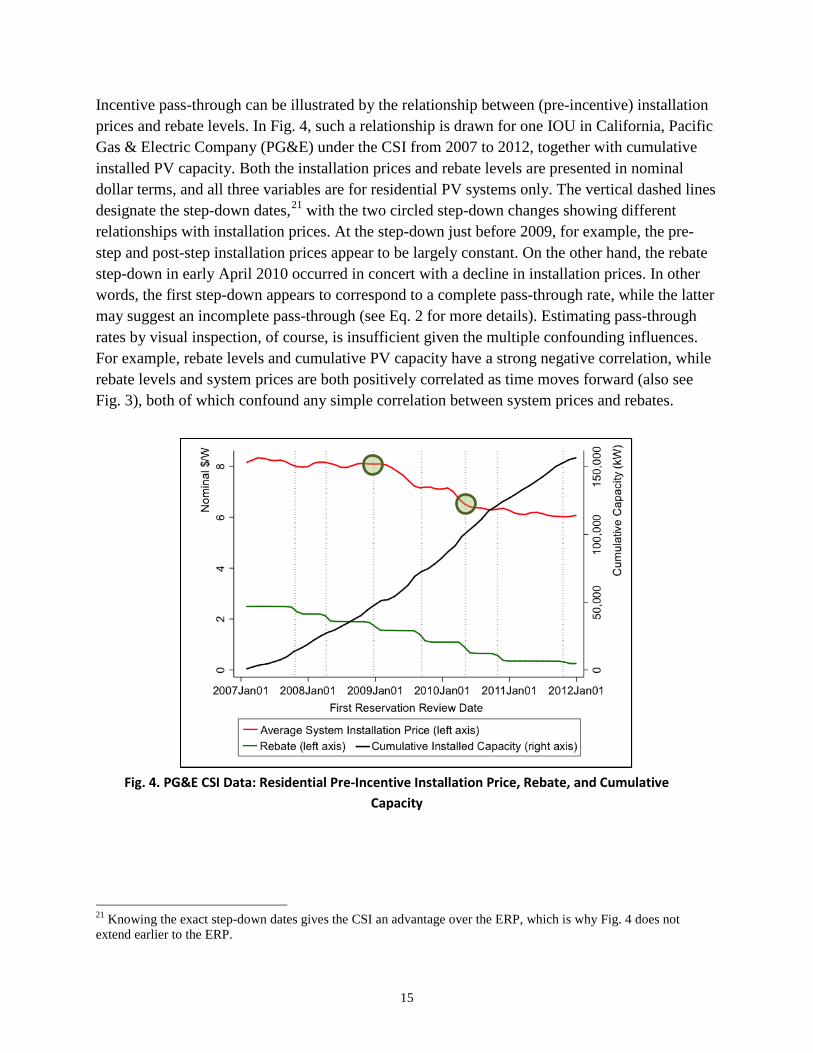
Incentive pass-through can be illustrated by the relationship between (pre-incentive) installation prices and rebate levels. In Fig. 4, such a relationship is drawn for one IOU in California, Pacific Gas & Electric Company (PG&E) under the CSI from 2007 to 2012, together with cumulative installed PV capacity. Both the installation prices and rebate levels are presented in nominal dollar terms, and all three variables are for residential PV systems only. The vertical dashed lines designate the step-down dates,21 with the two circled step-down changes showing different relationships with installation prices. At the step-down just before 2009, for example, the pre-step and post-step installation prices appear to be largely constant. On the other hand, the rebate step-down in early April 2010 occurred in concert with a decline in installation prices. In other words, the first step-down appears to correspond to a complete pass-through rate, while the latter may suggest an incomplete pass-through (see Eq. 2 for more details). Estimating pass-through rates by visual inspection, of course, is insufficient given the multiple confounding influences. For example, rebate levels and cumulative PV capacity have a strong negative correlation, while rebate levels and system prices are both positively correlated as time moves forward (also see Fig. 3), both of which confound any simple correlation between system prices and rebates.

21 Knowing the exact step-down dates gives the CSI an advantage over the ERP, which is why Fig. 4 does not extend earlier to the ERP.

Fig. 4. PG&E CSI Data: Residential Pre-Incentive Installation Price, Rebate, and Cumulative Capacity

15

Descriptive statistics are summarized in Table 1 (at the county-month level for the structural-modeling analysis) and Table 2 (at the system level for the reduced-form regression analysis). Both only include data used for the later analysis—i.e., systems in the 49 counties with the longest PV installation history in California.

Table 1. County-level Summary Statistics for Structural Modeling: 2001–2012

Variables (County Level) Mean Std. Dev. Min Max N

Installation price (real $/W) 8.50 1.94 2.71 21.48 5,677 Net price (real $/W) 6.19 1.23 0.20 18.24 5,677 Rebate (real $/W) 2.32 1.44 0.12 6.50 5,677 Monthly installation (kW) 80.36 150.3 0.58 1,799 5,677 TPO share 0.10 0.21 0 1 5,677 Summer season 0.50 0.50 0 1 5,677 # of zip codes 8.14 11.01 1 102 5,677 # of installers 6.92 8.89 1 69 5,677 Financial crisis year 0.09 0.29 0 1 5,677 Hardware cost (real $/W) 5.68 1.27 2.71 7.93 5,677 Labor cost (in $100,000)22 2.85 0.80 1.49 6.64 5,677

22 Note that the labor cost is inflated because in our weighting mechanism, we multiplied the wage for roofer and administrative by 2 and 2.5 respectively.

16

Table 2. System-level Summary Statistics for the Reduced-form Regression Analysis: 2001–2012

Variables (System Level) Mean Std. Dev. Min Max N Net price (real $/W) 6.211 1.865 2.4E-06 20.697 92,545 Installation Price (real $/W) 7.762 2.225 1.564 25.462 92,545 Rebate (real $/W) 1.551 1.304 0.074 8.825 92,545 System size (kW) 4.737 2.068 0.066 10 92,545 System size squared (kW2) 26.715 22.046 0.004 100 92,545 Residential system 0.990 0.098 0 1 92,545 Commercial system 0.006 0.080 0 1 92,545 Other customer segment 0.003 0.057 0 1 92,545 TPO23 0.235 0.424 0 1 92,545 China module 0.175 0.380 0 1 92,545 Micro-inverter 0.142 0.349 0 1 92,545 Thin-film 0.026 0.160 0 1 92,545 Building-integrated (BIPV) 0.003 0.059 0 1 92,545 Tracking system 0.001 0.025 0 1 92,545 Installer experience 0.325 4.475 0 195.84 92,545 Installer density 0.271 0.229 0 2.542 92,545 Hardware cost ($/W) 4.876 1.302 2.709 7.933 92,545 Labor cost (in $100,000) 3.264 0.894 1.488 6.640 92,545 Household income (≤ $24,999) 0.160 0.080 0.007 0.695 92,545 Household income ($25,000–$44,999) 0.155 0.058 0 0.581 92,545 Household income ($45,000–$99,999) 0.325 0.067 0.049 0.587 92,545 Household income (≥ $100,000) 0.360 0.152 0.009 0.859 92,545 Housing value (≤ $34,999) 0.024 0.028 0 0.361 92,545 Housing value ($35,000–$89,999) 0.039 0.052 0 0.663 92,545 Housing value ($90,000–$249,999) 0.193 0.192 0 0.886 92,545 Housing value (≥ $250,000) 0.743 0.242 0 1.000 92,545 Less than high school 0.060 0.059 0 0.601 92,545 High school without diploma 0.064 0.041 0 0.365 92,545 Less than bachelor 0.495 0.130 0 0.835 92,545 Bachelor degree or more 0.381 0.182 0 0.912 92,545 Occupied housing units (in 10,000) 3.388 1.769 0.001 10.389 92,545

The data show several additional noteworthy features that impacted our model specification. First, PV deployment appears to grow not only from the installed base within the same zip code (Bollinger and Gillingham, 2012; Rai and Robinson, 2013), but also over time expands from one zip code to another within a county, suggesting both intra- and inter-zip code diffusion effects.

23 Again, this is for non-appraised-value TPO PV systems only.

17

This is, in part, why we included both a lagged demand term and the number of zip codes in Eq. (11).24 Second, TPO market share increased over time. Under a TPO arrangement, a residential customer does not own the PV system, but instead hosts that system and purchases power from a third-party owner through a leasing or power-purchase agreement. In the reduced-form regression analysis, a TPO dummy variable was included, because TPO systems tended to show a slight price advantage relative to customer-owned systems, after excluding data for appraised-value systems. The growing attractiveness of TPO arrangements also needed to be controlled for in the demand equation of the structural modeling, as in Eq. (11).

4 Results In this section, we present results for structural modeling and then for the reduced-form regression analysis. As described above, in the structural modeling, we adopted two approaches: one as in Wolfram (1999) that estimates Eq. (11) first using 2SLS and then estimates Eq. (13’) (two-step estimation), and the other as proposed by Bresnahan (1982) that estimates Eq. (11) and Eq. (13’’) at the same time (one-step estimation). We conducted these two analyses for each county. For brevity in presentation, we only show detailed regression results for one of the largest PV-installation counties (San Diego), but we also present summary statistics (median and standard deviation) for the regression coefficients of all 49 counties analyzed. Reduced-form regression results at the system level were produced for California as a whole, pooling data from all 49 counties considered. Additionally, for those California counties with sufficient PV data (150 data points or more), county-level pass-through results are presented.

4.1 Structural Modeling

Focusing first on the structural modeling, Table 3 shows detailed regression results for San Diego county as well as summary statistics of the coefficients for all 49 counties in our analysis. These results are separated between the two-step estimation (Columns 1 and 2) and the one-step estimation (Columns 3 and 4). Results for the demand function are in Panel A, and results for the supply relation are in Panel B.

The first column of Panel A shows the regression results for PV demand in San Diego, based on the specification in Eq. (11) (two-step estimation). With monthly installed capacity in kW as the dependent variable, we instrumented the price term with 𝐻𝑎𝑟𝑑𝑤𝑎𝑟𝑒𝐶𝑜𝑠𝑡 and the price interaction term with a similar interaction term between 𝐻𝑎𝑟𝑑𝑤𝑎𝑟𝑒𝐶𝑜𝑠𝑡 and 𝑆𝑢𝑚𝑚𝑒𝑟, as discussed earlier. Unit-root and co-integration tests were conducted to make sure the relationship in the time series analysis is stable. Coefficients for the lagged capacity and price terms have the expected signs and are statistically significant. Without instrumenting, these two coefficients will

24 To see the motivation more clearly, define 𝑞𝑖𝑡 as the installed capacity within zip code 𝑖 and 𝑄𝑡 as the quantity for the whole county. Then, 𝑄𝑡 = ∑ 𝑞𝑖𝑡 =𝑖 ∑ (𝑞𝑖𝑡 − 𝑞�𝑡) + 𝑍𝑡𝑞�𝑡𝑖 , where 𝑞�𝑡 is the average installed capacity for all zip codes and 𝑍𝑡 is the number of zip codes, both at time 𝑡. Assume 𝑞𝑖𝑡 is a linear function of 𝑞𝑖,𝑡−1, thus, 𝑄𝑡 =𝑓(𝑄𝑡−1,𝑍𝑡).

18

be slightly deflated, indicating a potential downward bias. The positive coefficient of the lagged capacity variable suggests a penetration effect (or peer effects at this high geographic level), consistent with previous literature (Bollinger and Gillingham, 2012; Dong and Rai, 2014). Moreover, price has a negative coefficient (even after being instrumented), indicating that consumers respond to lower price as would be expected, even after controlling for penetration effects. Using mean system price and monthly demand, we calculate a PV price elasticity of demand of 0.3 in San Diego, which is smaller than found by Zhang et al. (2011) but is consistent with the findings of Rogers (2014); the difference compared to Zhang et al. (2011) may result from the fact that penetration effects were not considered in that study.

The positive coefficient of the price interaction term with 𝑆𝑢𝑚𝑚𝑒𝑟 indicates that PV consumers are less responsive to system prices during the two summer quarters. The negative coefficient for 𝑆𝑢𝑚𝑚𝑒𝑟, meanwhile, suggests that installations are lower in these months than in other months, all else being equal. As for other demand shifters, the prevalence of the TPO business model appears to attract more PV customer demand, consistent with Drury et al. (2012). As expected, the number of new markets in zip codes and number of installers in the market both contribute to higher PV adoption. Finally, the financial crisis is shown to have reduced PV demand in San Diego.

Looking across all 49 California counties in Column 2, qualitatively similar results are evident. Lagged capacity is found to be positively correlated with customer demand in 39 counties, while price is negatively correlated in 29 counties. For those counties with negative demand slope, the PV price elasticity of demand averages 0.6, with an absolute range of 0.08 to 1.9. 25 Results for the remaining variables were also broadly consistent with the results shown for San Diego, though with wide ranges in coefficient size due, in part, to differences in sample size.

Robustness tests were also done to control for other social-demographic variables, but those additional control variables did not change our main results, perhaps because they are largely captured already in the lagged capacity variable. We thus use the demand estimation results in Table 3 to impute the additional term (𝐻 = −�̂�𝑋/𝑄𝑃� ) and inject it into the supply-relation regression for calculating the pass-through rate.

Results for the supply-relation regression are shown in Column 1 in Panel B for San Diego, and in Column 2 for all 49 counties (two-step estimation). With the average system price as the dependent variable, the positive coefficient for capacity (installation scale in a month) suggests increasing prices with increasing market size in San Diego, all else being equal. Furthermore, hardware cost is passed through to installation prices, as would be expected. On the other hand, the increasing labor cost over time is negatively correlated with the simultaneously decreasing installation prices.

25 We did not differentiate the demand slope between summer quarters and other quarters when calculating demand elasticities. As with the San Diego results, we instrumented the price term with 𝐻𝑎𝑟𝑑𝑤𝑎𝑟𝑒𝐶𝑜𝑠𝑡.

19

As for the imputed term 𝐻 index, its coefficient can be roughly interpreted as the pricing response to the inverse of the absolute demand elasticity, and the small positive coefficient for San Diego means that lower demand elasticity tends to result in slightly higher prices. We then use the county-specific 𝐻 index results to calculate the conduct parameter 𝜃∗ = γ⁄(1-γ) and the pass-through rate based on Eq. (7). The estimate of 𝜃∗ in San Diego is relatively small, resulting from the small coefficient for the 𝐻 index. One way to interpret this result is that installers’ pricing behavior did not significantly exploit the (relatively small) demand elasticity but instead responded to other more obvious factors such as hardware cost changes and penetration effects. A small or statistically insignificant conduct parameter also generally implies a high pass-through rate, as detailed later.

Looking across all 49 counties in Column 2, for at least half of them, the negative coefficient for the capacity term indicates returns to scale—higher installation scale is correlated with lower prices. Other coefficients in the supply relation tend to have a similar magnitude as in San Diego, except for the labor-cost variable. Importantly, as with San Diego, the median value for the conduct parameter is small.

Turning to the one-step estimation in Columns 3 and 4, here we applied the Full Information Maximum Likelihood (FIML) estimation technique.26 Focusing first on the results for San Diego in Column 3, the one-step estimation coefficients are broadly consistent with the two-step results, but the generally smaller standard errors suggest greater estimation efficiency and precision. As with the two-step procedure, the conduct parameter is found to be very small. Results across all counties when using one-step estimation (Column 4) are similarly broadly consistent with the two-step estimation findings. The conduct parameter is found to be somewhat smaller than in the two-step estimation, and with a smaller standard deviation.

Fig. 5 shows county-specific pass-through results from the two-step estimation approach only; results are very similar using the one-step estimation process. The pass-through rates vary from 92% to 103% depending on local market conditions (Fig. 5a), generally with relatively narrow confidence bounds (Fig. 5b). A pass-through rate of 100% indicates that, on average, ERP and CSI incentives and incentive changes were fully passed through to consumers, and it suggests sufficient competition among installers in such local markets. A pass-through rate of less than 100%, on the other hand, suggests weaker competition among installers and that installers did not set prices based solely on their marginal costs. Overall, we find that average county-level pass-through rates have been high (99%). For the 49 counties included in this structural-modeling analysis, only five have pass-through rates estimated at less than 95%.

26 To implement FIML, we used the –nlsur– command in Stata with the –ifgnls– option; thanks to Kenneth Gillingham at Yale University for pointing us in this direction.

20

Table 3. Regression Output: PV Demand and Supply Relation for San Diego County and All Counties

Two-Step Estimation One-Step Estimation

San Diego All Counties San Diego All Counties27

(b/s.e.) (median/s.d.) (b/s.e.) (median/s.d.)

Panel A: Demand

Lagged Capacity 0.126* 0.106 0.153** 0.122

(0.066) (0.161) (0.061) (0.164) Price -21.745* -0.564 -14.831*** -1.550

(11.531) (6.258) (1.472) (2.825) Price × Summer 30.054** 0.812 33.707*** 0.291 (13.278) (5.892) (9.441) (7.538) Summer -286.707** -5.911 -319.685*** -2.116

(121.859) (55.885) (88.623) (71.829) TPO Ratio 501.526*** 8.368 487.958*** 12.359

(103.138) (98.899) (94.209) (110.914) # of Zip Codes 9.823*** 6.266 9.384*** 6.395

(1.236) (3.093) (1.167) (2.393) # of Installers 4.385*** 3.622 4.890*** 2.688

(1.323) (2.131) (1.240) (1.918) Financial Crisis Year -68.569*** -2.125 -55.427*** -2.656

(17.121) (13.880) (16.906) (14.320)

Panel B: Supply Relation

Capacity (𝜎1) 0.0007*** -0.0060 0.0014*** -0.0011 (0.0003) (0.0287) (0.0003) (0.0471) Hardware Cost 1.211*** 1.204 1.392*** 1.169 (0.117) (0.258) (0.110) (0.295) Labor Cost -1.087 -0.159 -0.652 -0.158 (0.718) (1.150) (0.687) (0.989) H Index (𝛾) 0.0010 0.0010 (0.0008) (0.0301) Conduct Parameter (𝜃∗) 0.0010 0.0010 0.0006 0.0004 (0.0008) (0.0333) (0.0010) (0.0134)

N 144 49 144 33

Robust standard errors are in parentheses for the first and third columns, while standard deviations are in parentheses for the second and fourth columns; the constant term is suppressed; * p<0.10, ** p<0.05, *** p<0.01.

27 Note that the sample size (33 counties) is lower in the one-step estimation; this is because limited sample size in 16 counties led to the estimation procedure in Stata not converging in this case.

21

(a) Estimated Pass-through Rates

(b) 95% Confidence Intervals for Pass-through Rates

Fig. 5. Pass-through Rates for 49 California Counties: Structural-Modeling Approach

22

A key reason for the relatively high pass-through rates is that the conduct parameters, as discussed earlier, are generally found to be small and close to zero.28 The conduct parameters can also be inverted to obtain the numbers of “equivalent” firms29 competing in the relevant PV market. For the 33 counties with positive conduct parameters, the median number of equivalent firms is 138, suggesting a reasonably high level of market competition. Nonetheless, in some counties only seven or eight equivalent firms have competed for customers, leading to somewhat lower pass-through rates.

4.2 Reduced-form Approach

As described in Section 3.2, the reduced-form approach consists of two versions of the same regression, both at the system level. One pools systems from all counties together, and the other is run for each county. We first show regression results for the all-counties case and then discuss the county-specific results.

Table 4 summarizes the regression results based on Eq. (14), with different sets of fixed effects added: M1 only contains zip code fixed effects, M2 only uses monthly fixed effects (and, accordingly, the hardware and labor cost terms are dropped, as these also are defined by time), and M3 includes zip code × month fixed effects. All models include social-demographic variables, the results of which are not presented here owing to space constraints, and all standard errors are clustered at the zip code level in order to account for series correlation in the error term.

The key variable of interest is the rebate level, and our estimates show reasonably consistent results on the pass-through rate across all three reduced-form models, M1–M3, ranging from 86% to 103%. These average pass-through rates are also consistent with the results from the structural modeling, suggesting a relatively robust model specification. Based on our evaluation of the CSI/ERP programs, it would appear that rebates have largely been passed through to PV customers. Though not shown here, similar results are found when we limit the data sample to the CSI only or when we drop all TPO systems, not only appraised-value TPO systems. To be clear, because appraised-value TPO systems are necessarily excluded in all cases, our results cannot speak to pass-through rates among TPO systems broadly.30

28 The conduct parameter coefficient remains small and close to zero even when we pool all of the counties together. This suggests that the small coefficient here is not due to small sample size. 29 The number of equivalent firms is positively correlated with the actual number of firms across markets. 30 Non-appraised-value TPO systems report pricing based on transactions between installers and third-party owners, not between installers and end-use PV customers. As such, to the extent our results address pass-through for non-appraised-value TPO systems, it is the pass-through from the installer to the third-party leasing company (rather than to the actual host customer).

23

Table 4. System-level Regression Results for 49 California Counties Together

Dependent variable: net price (real $/W) M1 M2 M3 Rebate -0.940*** -0.855*** -1.033***

(0.025) (0.038) (0.037) System size -0.942*** -0.921*** -0.950***

(0.035) (0.033) (0.050) System size squared 0.066*** 0.064*** 0.066***

(0.003) (0.003) (0.004) Commercial systems 0.038 0.096 0.133 (0.099) (0.099) (0.196) Other segments 0.735*** 0.706*** 0.760***

(0.133) (0.133) (0.267) TPO -0.323*** -0.299*** -0.267*** (0.029) (0.036) (0.044) China module -0.546*** -0.532*** -0.634*** (0.022) (0.027) (0.035) Micro-inverter 0.458*** 0.516*** 0.476***

(0.032) (0.035) (0.053) Thin-film 0.400*** 0.225*** 0.284***

(0.057) (0.057) (0.100) Building-integrated (BIPV) 0.423*** 0.384*** 0.352

(0.134) (0.118) (0.262) Tracking system 1.288*** 1.234*** 1.640*** (0.288) (0.306) (0.577) Installer experience -0.010*** -0.013*** -0.009*

(0.003) (0.003) (0.006) Installer density -0.197** -0.794*** 0.156

(853.9) (661.5) (4785.8) Hardware cost 0.938*** (0.019) Labor cost -0.151*** (0.033) Social-demographic variables Yes Yes Yes Zip code fixed effects Yes Monthly fixed effects Yes Zip code × month fixed effects Yes N 92,545 92,545 92,545 Adjusted R2 0.322 0.297 0.464 Model degree of freedom 25 24 13

Note: Zip code clustered standard errors are in parentheses; * p<0.10, ** p<0.05, *** p<0.01; social-demographic control variables are not reported owing to space constraints.

Results for some of the control variables in Table 4 are also noteworthy. For example, hardware cost in M1 has a coefficient around 1, which suggests that hardware cost pass-through rates are almost complete. System size and its squared term have coefficients showing diminishing

24

economies of scale with increasing system size, as one would expect. Non-appraised-value TPO systems may have some price advantage, relative to non-TPO systems. Systems with Chinese modules have relatively lower prices, as would be expected. Similarly, systems using micro-inverters, thin-film modules, trackers, or BIPV tend to have higher prices. On the other hand, installer experience reduces installation prices, presumably owing to within-firm learning-by-doing. Higher installer density also tends to correlate with lower installation prices.

The same system-level regression in Eq. (14) can be run for each county, thus forming an interesting comparison with the county-level structural-modeling results. Focusing only on the 42 counties with 150 or more PV installations, Fig. 6 presents the pass-through results of this county-level analysis. In particular, the figure plots all pass-through estimates for M1–M3 that are found to be statistically significant, with t-statistics no smaller than 2.36. In total, statistically significant results are found for 36 counties in M1, 28 counties in M2, and 23 counties in M3. As shown, the overall results tend to center around a 100% pass-through rate, consistent with our previous estimates. In particular, the county-level weighted average (by the number of systems included in a county) pass-through rate is estimated at 95%. A more significant spread is found among counties, however, with pass-through rate estimates as low as 32% and as high as 270%, depending on the model. Some of this range may be due to limited sample size: focusing on the inner 10th-90th percentile of pass-through results, the range narrows to 68% to 122%.

Note: counties with less than 150 installed PV systems were excluded.

Fig. 6. System-level Regression Results for County-specific Pass-through Rates

25

5 Conclusions

We find a high overall historical pass-through rate for the California residential PV rebate programs, though with some level of heterogeneity among counties. The structural-modeling approach estimates county-level pass-through rates that vary from 92% to 103%, with a mean value of 99%. The reduced-form regression analysis finds consistent results, with average pass-through rates ranging from 86% to 103% at the state level and with a county-level average pass-through rate of 95%. Focusing on the inner 10th-90th percentile of reduced-form pass-through results at the county level, a range of 68% to 122% is estimated. We consider these two approaches to be complementary: while the structural-modeling approach has a strong theoretical basis and can produce reliable results for relatively small markets, the reduced-form regression analysis is straightforward, easy to interpret, and does not require as many structural assumptions. Moreover, a forthcoming companion paper that relies on RD designs similarly estimates high pass-through rates among the California solar incentive programs. The similarity of results from these various approaches to estimating pass-through rates lends credibility and robustness to those results.

In general, these results suggest that PV installers in California have considered CSI and ERP rebates as exogenous factors when making pricing decisions, and they suggest a reasonably competitive market and, at least from the perspective of incentive pass through, a well-functioning subsidy program. In part, these results may be due to the fact that California’s rebate changes over time have been somewhat gradual, especially under the CSI, with each step-down representing a relatively small drop in the level of the state incentive. There may be little opportunity or motivation for installers to manipulate their pricing behavior in response to such small and somewhat-gradual rebate changes. These results may also suggest that installers have been competing more on quantity than on price, taking rebate step-downs as an opportunity to increase sales in advance of the step-down—a result consistent with that found in Gürtler and Sieg (2009) and Hughes and Podolefsky (2013).

Our high pass-through results stand in apparent contrast to those of other authors. Podolefsky (2013), for example, finds a rather low incentive pass-through rate for the federal ITC for residential PV. This lower estimated pass-through rate may be due to the relatively larger and more-abrupt changes in the federal incentive, over time, in comparison to the CSI. Similarly, Wiser et al. (2007) analyzed pass-through in California based solely on the earlier ERP, finding pass-through rates of well below 100%. In part this result may be due to suboptimal model specification. In addition, the ERP experienced more-abrupt and sizable changes in incentive levels than the CSI, and it was in place when the solar market in California was less mature; this may help explain some of the discrepancy with the present results. Finally, our results appear to contrast with those presented in Henwood (2014). A key reason may be the different model specifications and different control variable sets: for example, though Henwood used utility-level fixed effects, we included zip code fixed effects; and while Henwood only controlled for TPO

26

systems versus non-TPO systems, we included a large number of other system characteristics as important controls.

Though we find—using multiple methods—a high level of historical incentive pass-through in California, it is important to be careful in making broad inferences based on these results. Our focus has been on residential PV systems in California, and we have excluded appraised-value TPO PV systems. As a result, the pass-through rates estimated here do not apply outside of California, and they do not apply fully to all TPO PV systems. Additionally, our results focus narrowly on the pass-through rate for direct solar incentives offered by the CSI and ERP. We do not evaluate so-called “value-based pricing” more broadly, which would necessarily consider the combined impact of direct state incentives, electric utility bill savings, and federal tax incentives.

Given these and other limitations, several additional areas of further research on incentive pass-through are warranted, both to assess the robustness of the present results and to judge their applicability in other market contexts. First, the reduced-form model results presented here may suffer from several forms of model bias. Use of RD design (as in our companion, forthcoming paper) to judge PV system pricing across temporal or geographic boundaries may help improve the precision of our estimates of incentive pass-through rates. Second, though the present results focus entirely on California’s PV incentive programs, other states have also developed a wide range of policy mechanisms to support solar market development. Assessments of incentive pass-through in markets outside of California—at the state and federal levels—would help improve our understanding of the robustness of the present results as well as the conditions under which pass-through rates are relatively higher or lower. Third, the current work focuses on the pass-through of California’s CSI and ERP rebates, but PV customers benefit from PV through various other means as well, for example, the federal ITC, retail electric bill reductions, and sales of solar renewable energy certificates. As such, a more comprehensive evaluation of value-based pricing, considering all of these factors, is warranted. Finally, owing to data limitations, the analysis presented in this report focuses on customer-owned PV systems and non-appraised-value TPO systems. Further research is warranted to illuminate incentive pass-through and value-based pricing among all TPO systems, especially given the recent growth in the market for such systems.

27

References Alexeeva-Talebi, V., 2011. Cost Pass-through of the EU Emissions Allowances: Examining the

European Petroleum Markets. Energy Economics 3, S75–S83.

Ardani, K., Barbose, G., Margolis, R., Wiser, R., Feldman, D., Ong, S., 2012. Benchmarking Non-Hardware Balance of System (Soft) Costs for U.S. Photovoltaic Systems Using a Data-Driven Analysis from PV Installer Survey Results. National Renewable Energy Laboratory, Golden, CO; Lawrence Berkeley National Laboratory, Berkeley, CA.

Barbose, G., Darghouth, N., Weaver, S., Wiser, R., 2013. Tracking the Sun VI: An Historical Summary of the Installed Price of Photovoltaics in the United States from 1998 to 2012. Lawrence Berkeley National Laboratory, Berkeley, CA.

Barnett P.G., Keeler, T.E., Hu T., 1995. Oligopoly Structure and the Incidence of Cigarette Excise Taxes. Journal of Public Economics 57, 457–470.

Bergin, P., Feenstra, R.C., 2009. Pass-through of Exchange Rates and Competition Between Fixers and Floaters. Journal of Money, Credit and Banking 41(s1), 35–70.

Berry, S., Levinsohn, J., Pakes, A., 1995. Automobile Prices in Market Equilibrium. Econometrica 63, 841–889.

Besley, T.J., Rosen, H.S., 1999. Sales Taxes and Prices: An Empirical Analysis. National Tax Journal 52(2), 157–178.

Bettendorf, L., Verboven, F., 2000. Incomplete Transmission of Coffee Bean Prices: Evidence from the Netherlands. European Review of Agricultural Economics 27(1), 1–16.

Bezdek, R.H., 1993. The Environmental, Health, and Safety Implications of Solar Energy in Central Station Power Production. Energy 18(6), 681–685.

Bollinger, B., Gillingham, K., 2012. Peer Effects in the Diffusion of Solar Photovoltaic Panels. Marketing Science 31(6), 900–912.

Bresnahan T.F., 1982. The Oligopoly Solution Concept is Identified. Economics Letters 10, 87–92.

Brownlee, O., Perry, G., 1967. The Effects of the 1965 Federal Excise Tax Reduction on Prices. National Tax Journal 20(3), 235–249.

Burr, C., 2012. Subsidies, Tariffs and Investment in the Solar Power Market [WWW Document]. URL http://econ.arizona.edu/docs/JobMarket/burr_jobmarket12.pdf

Busse, M., Silva-Risso, J., Zettelmeyer, F., 2006. $1,000 Cash Back: The Pass-Through of Auto Manufacturer Promotions. American Economic Review 96, 1253–1270.

Carbonnier C., 2007. Who Pays Sales Taxes? Evidence from French VAT Reforms, 1987–1999. Journal of Public Economics 91, 1219–1229.

Choudhri, E., Hakura, D., 2012. The Exchange Rate Pass-Through to Import and Export Prices: The Role of Nominal Rigidities and Currency Choice. IMF Working Papers, WP/12/226.

Clay, K., Troesken, W., 2003. Further Tests of Static Oligopoly Models: Whiskey, 1882–1898. The Journal of Industrial Economics 51(2), 151–166.

28

Corts, K.S., 1999. Conduct Parameters and the Measurement of Market Power. Journal of Econometrics 88(2), 227–250.

CPUC (California Public Utilities Commission), 2014. California Solar Initiative Program Handbook [WWW Document]. URL http://www.gosolarcalifornia.ca.gov/documents/CSI_HANDBOOK.PDF

Davidson, C., Steinberg, D., 2014. Evaluating the Impact of Third-Party Price Reporting and Other Drivers on Residential Photovoltaic Price Estimates. Energy Policy 62, 752–761.

Delipalla, S., Keen, M., 1992. The Comparison between Ad Valorem and Specific Taxation under Imperfect Competition. Journal of Public Economics 49, 351–367.

Dixon, H.D., Somma, E.S., 2003. The Evolution of Consistent Conjectures. Journal of Economic Behavior & Organization 51, 523–536.

Dong, C.G., Rai, V., 2014. Optimal Subsidy Design under Uncertainty: A Dynamic Programming Evaluation of the California Solar Initiative. Presented at the 37 USAEE Conferences, New York, June 15–18, 2014.

Drury, E., Miller, M., Macal, C.M., Graziano, D.J., Heimiller, D., Ozik, J., Perry IV, T.D., 2012. The Transformation of Southern California’s Residential Photovoltaic Market through Third-Party Ownership. Energy Policy 42, 681–990.

Due, J.F., 1954. The Effect of the 1954 Reduction in Federal Excise Taxes on the List Prices of Electrical Appliances. National Tax Journal 7(3), 222–226.

EPIA, 2014. Global Market Outlook for Photovoltaics: 2014–2018. European Photovoltaic Industry Association, Brussels, Belgium.

Genesove, D., Mullin, W., 1998. Testing Static Oligopoly Models: Conduct and Cost in the Sugar Industry, 1890–1914. RAND Journal of Economics 29(2), 355–377.

Gopinath, G., Itskhoki, O., Rigobon, R., 2010. Currency Choice and Exchange Rate Pass-through. American Economic Review 100(1), 304–336.

Gron, A., Swenson, D., 2000. Cost Pass-Through in the U.S. Automobile Market. The Review of Economics and Statistics 82(2), 316–324.

Gürtler, M., Sieg, G., 2009. Crunch Time: A Policy to Avoid the ‘Announcement Effect’ when Terminating a Subsidy. German Economic Review 11(1), 25–36.

Fullerton, D., Metcalf, G.E., 2002. Tax Incidence. In Alan J. Auerbach and Martin Feldstein (eds.), Handbook of Public Economics. Elsevier, 1787–1872.

Hendricks, N., Janzen, J., Dhuyvetter, K., 2012. Subsidy Incidence and Inertia in Farmland Rental Markets: Estimates from a Dynamic Panel. Journal of Agricultural and Resource Economics 37(3), 361–378.

Henwood, K., 2014. Subsidy Pass-through in Residential Solar Markets [WWW Document]. URL http://home.uchicago.edu/~/keithjhenwood/PTv5.pdf

Hughes, J.E., Podolefsky, M., 2013. Getting Green with Solar Subsidies: Evidence from the California Solar Initiative [WWW Document]. URL http://spot.colorado.edu/~jonathug/Jonathan_E._Hughes/Main_files/PV_Subsidies.pdf

29

Jaffe, S., Weyl, E.G., 2013. The First-Order Approach to Merger Analysis. The American Economic Journal: Microeconomics 5(4), 188–218.

Karp, L., Perloff, J., 1989. Estimating Market Structure and Tax Incidence: The Japanese Television Market. Journal of Industrial Economics 37(3), 225–239.

Kim, D., Cotterill, R.W., 2008. Cost Pass-Through in Differentiated Product Markets: The Case of U.S. Processed Cheese. Journal of Industrial Economics 56(1), 32–48.

Kirwan, B.E., 2009. The Incidence of U.S. Agricultural Subsidies on Farmland Rental Rates. Journal of Political Economy 117, 138–164.

MacKay, A., Miller, N.H., Remer, M., Sheu, G., 2014. Bias in Reduced-Form Estimates of Pass-Through. Economics Letters 123(2), 200–202.

Marazzi, M., Sheets N., Vigfusson, R.J., Faust, J., Gagnon, J.E., Marquez, J., Martin, R.F., Reeve, T.A., Rogers, J.H., 2005. Exchange Rate Pass-through to U.S. Import Prices: Some New Evidence. Board of Governors of the Federal Reserve System International Finance Discussion Paper No. 833.

Marion, J., Muehlegger, E., 2011. Fuel Tax Incidence and Supply Conditions. Journal of Public Economics 95, 1202–1212.

McDonald, A., Schrattenholzer, L., 2001. Learning Rates for Energy Technologies. Energy Policy 29(4), 255–261.

Painuly, J.P., 2002. Barriers to Renewable Energy Penetration: A Framework for Analysis. Renewable Energy 24(2), 73–89.

Peterman, C.J., 2012. Subsidy Pass-through for PV Customers. Presented at EI Camp, Berkeley, CA.

Podolefsky, M., 2013. Tax Evasion and Subsidy Pass-Through under the Solar Investment Tax Credit [WWW Document]. URL http://www.colorado.edu/economics/papers/Wps-13/wp13-05/wp13-05.pdf

Possajennikov, A., 2009. The Evolutionary Stability of Constant Consistent Conjectures. Journal of Economic Behavior & Organization 72, 21–29.

Poterba, J.M., 1996. Retail Price Reactions to Changes in State and Local Sales Taxes. National Tax Journal 49(2), 165–176.

Rachapalli, S.R., Kulshreshtha, P., 2013. Evolutionarily Stable Conjectures and Social Optimality in Oligopolies. Theoretical Economics Letters 3, 12–18.

Rai, V., Robinson, S.A., 2013. Effective Information Channels for Reducing Costs of Environmentally- Friendly Technologies: Evidence from Residential PV Markets. Environmental Research Letters 8(1), 014044.

Reiss, P.C., Wolak, F.A., 2007. Structural Econometric Modeling: Rationales and Examples from Industrial Organization. In James J. Heckman and Edward E. Leamer (eds.), Handbook of Econometrics, Volume 6A. Amsterdam and Oxford: Elsevier, North-Holland, 4277–4415.

Rogers, E., 2014. Effectiveness of Capacity-Dependent Rooftop Solar Subsidies: Lessons from California. North Carolina State University, working paper.

30

Sallee, J.M., 2011. The Surprising Incidence of Tax Credits for the Toyota Prius. American Economic Journal: Economic Policy 3, 189–219.

SEIA/GTM, 2014. U.S. Solar Market Insight Report: 2013 Year-in-Review. GTM Research and Solar Energy Industries Association.

Sherwood, L., 2013. U.S. Solar Market Trends 2012. Interstate Renewable Energy Council, Inc., Latham, NY.

Shrimali, G., Jenner, S., 2013. The Impact of State Policies on Deployment and Cost of Solar PV in the US: A Sector Specific Empirical Analysis. Renewable Energy 60, 679–690.

Sijm, J., Chen, Y., Hobbs, B.F., 2012. The Impact of Power Market Structure on CO2 Cost Pass-Through to Electricity Prices under Quantity Competition – A Theoretical Approach. Energy Economics 34, 1143–1152.

Stern, N., 1987. The Effects of Taxation, Price Control and Government Contracts in Oligopoly and Monopolistic Competition. Journal of Public Economics 32, 133–158.

Timmins, C., Schlenker, W., 2009. Reduced Form versus Structural Modeling in Environmental and Resource Economics. Annual Review of Resource Economics 1(1), 351–380.

van Benthem, A., Gillingham, K., Sweeney, J., 2008. Learning-by-Doing and the Optimal Solar Policy in California. Energy Journal 29, 131–151.

Vavra, P., Goodwin, B.K., 2005. Analysis of Price Transmission Along the Food Chain. OECD Food, Agriculture and Fisheries Working Papers, No. 3, OECD Publishing.

Vivid Economics, 2007. A Study to Estimate Ticket Price Changes for Aviation in the EU ETS [WWW Document]. URL http://www.vivideconomics.com/uploads/reports/a-study-to-estimate-ticket-price-changes-for-aviation-in-the-eu-ets/Vivid_Econ_Aviation_Tickets.pdf

Weyl, G., Fabinger, M., 2013. Pass-Through as an Economic Tool: Principle of Incidence under Imperfect Competition. Journal of Political Economy 121(3), 528–583.

Wiser, R., Bolinger, M., Cappers, P., Margolis, R., 2007. Analyzing Historical Cost Trends in California’s Market for Customer-Sited Photovoltaics. Progress in Photovoltaics: Research and Applications 15(1), 69–85.

Wolfram, C., 1999. Measuring Duopoly Power in the British Electricity Spot Market. The American Economics Review 89(4), 805–826.

Woodard, F.O., Siegelman, H., 1967. Effects of the 1965 Excise Tax Reduction upon the Prices of Automotive Replacement Parts. National Tax Journal 20(3), 250–258.

Zhang, Y., Song, J., Hamori, S., 2011. Impact of Subsidy Policies on Diffusion of Photovoltaic Power Generation. Energy Policy 39, 1958–1964.

31

AcknowledgmentsKey Report ContactsThe work described in this paper was funded by the Office of Energy Efficiency and Renewable Energy (Solar Energy Technologies Office) of the U.S. Department of Energy (DOE) under Contract No. DE-AC02-05CH11231. For reviewing earlier versions of this work or providing valuable input, we would particularly like to thank Galen Barbose and Naïm Darghouth (LBNL); Kenneth Gillingham, Hao Deng,Paige Weber, Hilary Staver, and Tsvetan Tsvetanov (Yale University); Gregory Nemet (University of Wisconsin-Madison); David Arfin (First Energy Finance; and Merideth Sterkel (California Public Utilities Commission). For their support of this work, we also thank Elaine Ulrich, Christina Nichols, Joshua Huneycutt, and Minh Le of the DOE. Of course, the authors are solely responsible for any omissions or errors contained herein.

Ryan Wiser, Lawrence Berkeley National Laboratory (LBNL)rhwiser@lbl.gov

C.G. Dong, University of Texas at Austincgdong@utexas.edu

Varun Rai, University of Texas at Austinvarun.rai@mail.utexas.edu

Download the Reporthttp://emp.lbl.gov/reports

DisclaimerThis document was prepared as an account of work sponsored by the United States Government. While this document is believed to contain correct information, neither the United States Government nor any agency thereof, nor The Regents of the University of California, nor any of their employees, makes any warranty, express or implied, or assumes any legal responsibility for the accuracy, completeness, or usefulness of any information, apparatus, product, or process disclosed, or represents that its use would not infringe privately owned rights. Reference herein to any specific commercial product, process, or service by its trade name, trademark, manufacturer, or otherwise, does not necessarily constitute or imply its endorsement, recommendation, or favoring by the United States Government or any agency thereof, or The Regents of the University of California. The views and opinions of authors expressed herein do not necessarily state or reflect those of the United States Government or any agency thereof, or The Regents of the University of California.

Ernest Orlando Lawrence Berkeley National Laboratory is an equal opportunity employer.

October 2014