income and substitution effects
DESCRIPTION
Income and Substitution Effects. The Law of Demand:. Slope of budget line from p x / p y to steeper p x ’/ p y. y. p x / p y. U 1. U 2. p x ’/ p y. p x / p y. x * =x( p x ,p y ,M ). x. x. x b. x a. x b. x a. Qd falls from x a to x b. Qd falls from x a to x b. - PowerPoint PPT PresentationTRANSCRIPT
Income and Substitution Effects
The Law of Demand:x
x
p
y
xb xa xb xa
x*=x(px,py,M)
U1U2
x x
px/py
px/py
px’/py
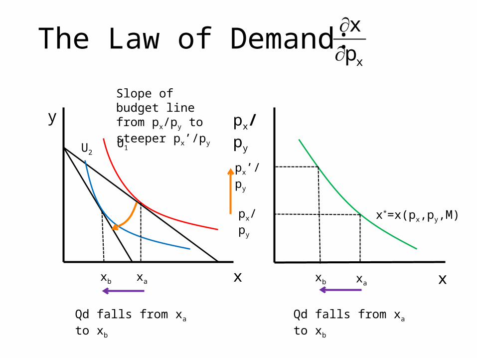
Slope of budget line from px/py to steeper px’/py
Qd falls from xa to xbQd falls from xa to xb
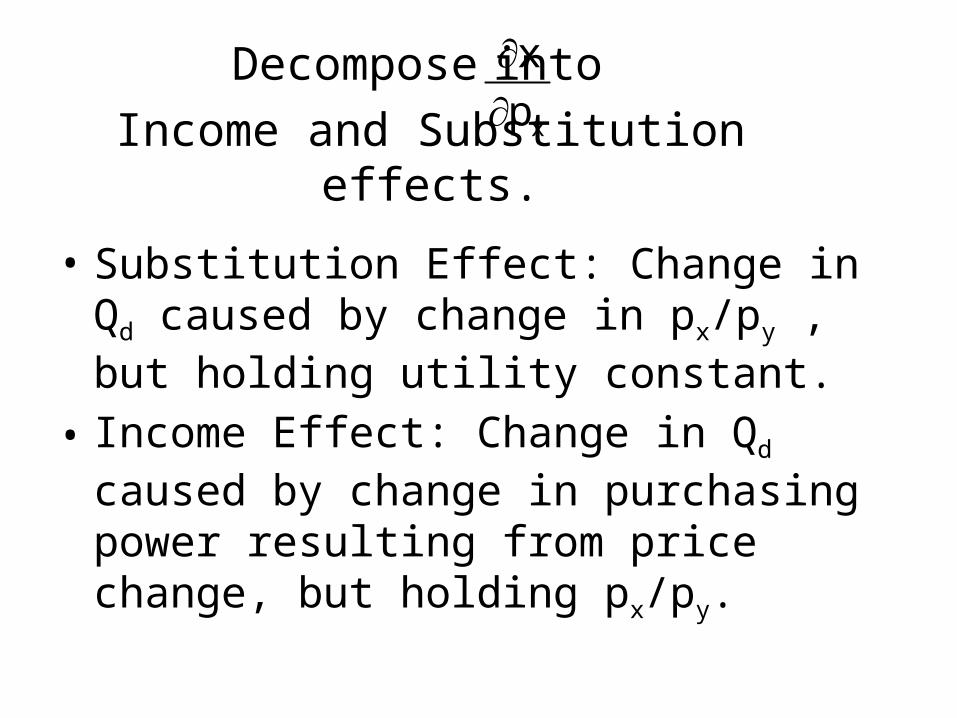
• Substitution Effect: Change in Qd caused by change in px/py , but holding utility constant.
• Income Effect: Change in Qd caused by change in purchasing power resulting from price change, but holding px/py.
Decompose into Income and Substitution effects.
x
x
p
Substitution Effect
y
xb xa xbxa
x*=x(px,py,M)
U1
x x
px/py
px/py
px’/py
Substitution effect: How Qd changes as a result of the price change, even when utility can be held constant (Qd from xa to xc)
xcxc
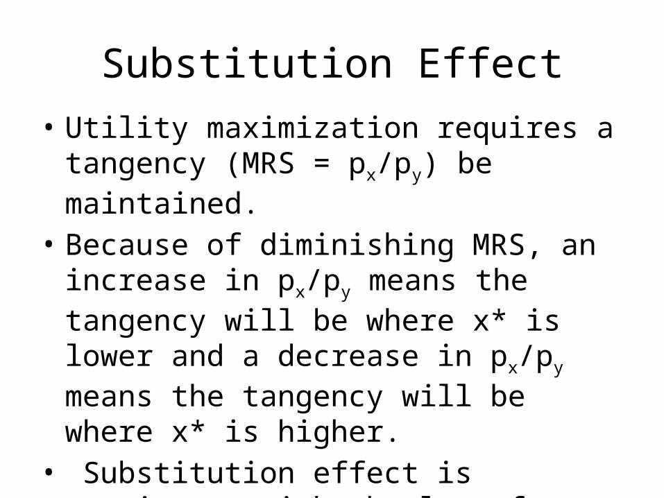
Substitution Effect• Utility maximization requires a tangency (MRS
= px/py) be maintained.• Because of diminishing MRS, an increase in
px/py means the tangency will be where x* is lower and a decrease in px/py means the tangency will be where x* is higher.
• Substitution effect is consistent with the law of demand.
Income Effect
y
xb xbxa
x*=x(px,py,M)
U1
x x
px/py
px/py
px’/py
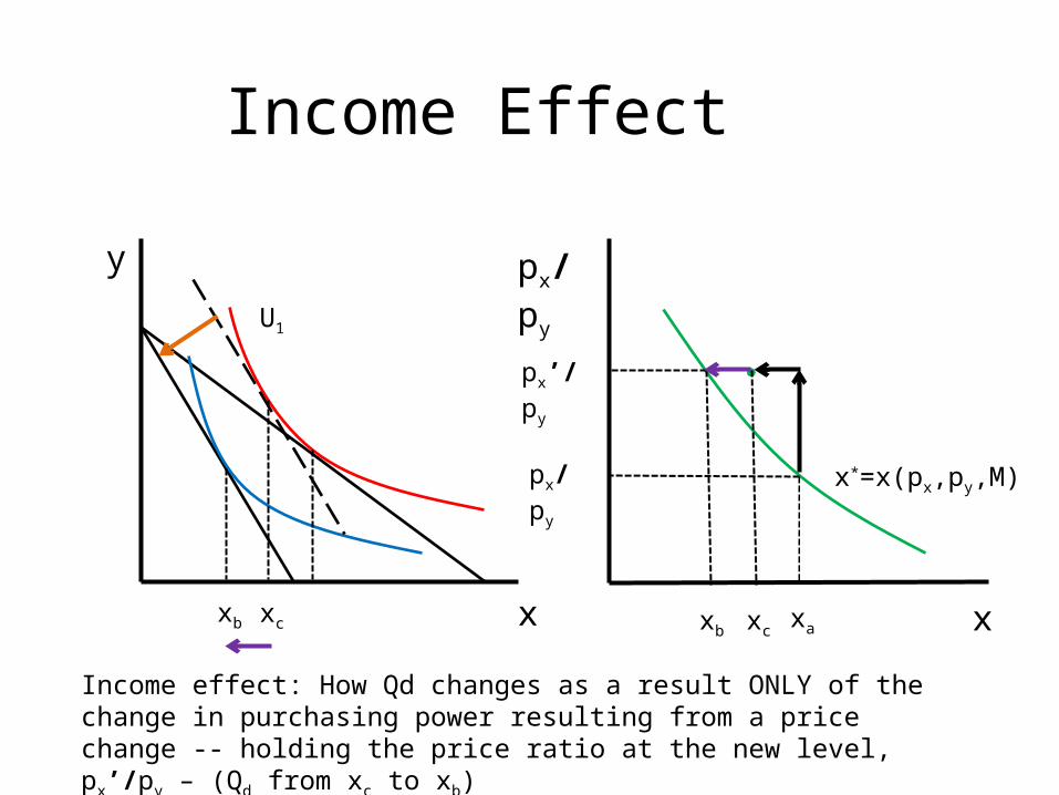
Income effect: How Qd changes as a result ONLY of the change in purchasing power resulting from a price change -- holding the price ratio at the new level, px’/py – (Qd from xc to xb)
xcxc
Income Effect• By isolating the change in purchasing power (but
leaving the price ratio unchanged), the income effect looks exactly like the change resulting from a change in income.
• Normal goods, increase in price means decrease in purchasing power, so income effect is negative– reinforces the law of demand.
• Inferior goods, increase in price means decrease in purchasing power, so income effect is positive – runs counter to the law of demand.
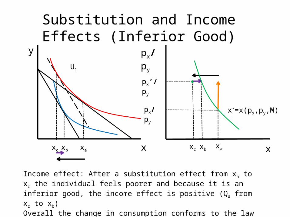
Substitution and Income Effects (Inferior Good)
y
xbxb
xa
x*=x(px,py,M)
U1
x x
px/py
px/py
px’/py
Income effect: After a substitution effect from xa to xc the individual feels poorer and because it is an inferior good, the income effect is positive (Qd from xc to xb)Overall the change in consumption conforms to the law of demand unless the good is inferior and the income effect so large that it overwhelms the substitution effect. Goods for which this occurs are called Giffen goods.
xcxc xa
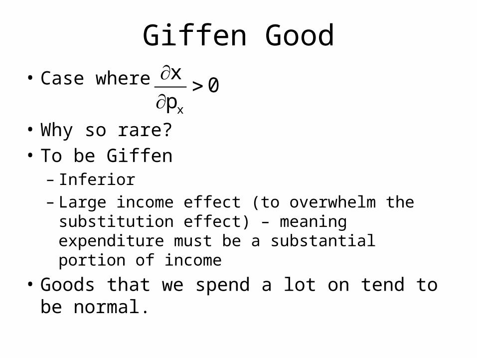
Giffen Good• Case where
• Why so rare? • To be Giffen
– Inferior– Large income effect (to overwhelm the substitution
effect) – meaning expenditure must be a substantial portion of income
• Goods that we spend a lot on tend to be normal.
x
x0
p
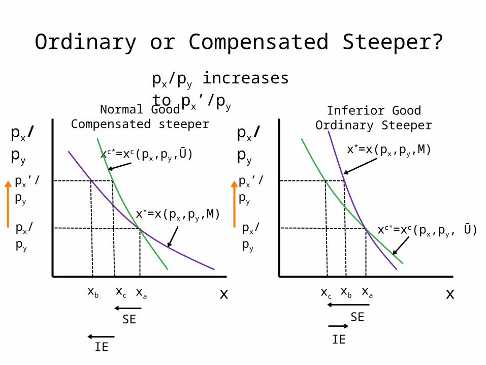
Ordinary or Compensated Steeper?
xa
xc*=xc(px,py, Ū)
x
px/py
px/py
px’/py
px/py increases to px’/py
xcxa
xc*=xc(px,py,Ū)
x
px/py
px/py
px’/py
xc
Normal GoodCompensated steeper
Inferior GoodOrdinary Steeper
xb
x*=x(px,py,M)
xb
x*=x(px,py,M)
SE
IE
SE
IE
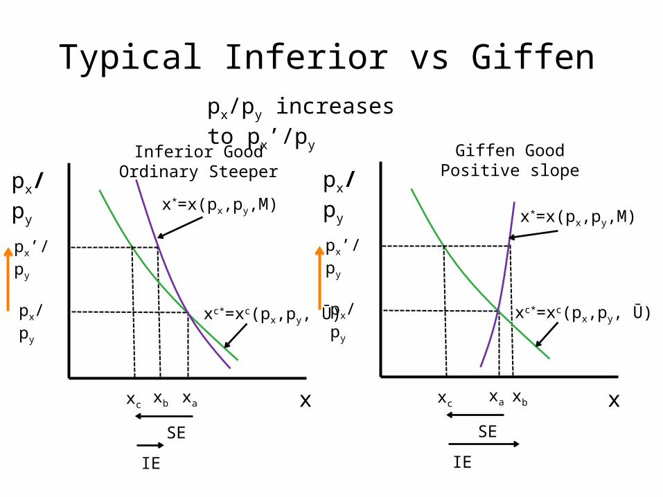
Typical Inferior vs Giffen
xa
xc*=xc(px,py, Ū)
x
px/py
px/py
px’/py
px/py increases to px’/py
xcx
Giffen GoodPositive slope
xb
x*=x(px,py,M)
SE
IE
xa
xc*=xc(px,py, Ū)
px/py
px/py
px’/py
xc
Inferior GoodOrdinary Steeper
xb
x*=x(px,py,M)
SE
IE
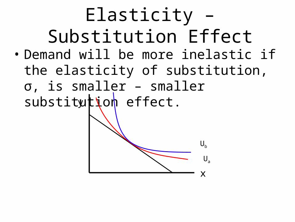
Elasticity – Substitution Effect• Demand will be more inelastic if the elasticity of
substitution, σ, is smaller – smaller substitution effect.
y
Ua
x
Ub
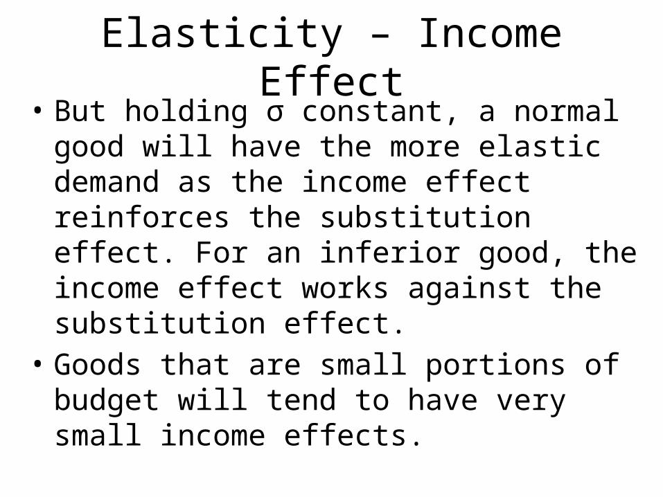
Elasticity – Income Effect• But holding σ constant, a normal good will have
the more elastic demand as the income effect reinforces the substitution effect. For an inferior good, the income effect works against the substitution effect.
• Goods that are small portions of budget will tend to have very small income effects.
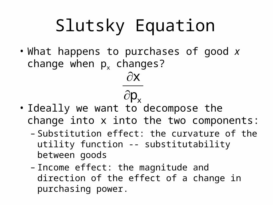
Slutsky Equation• What happens to purchases of good x change
when px changes?
• Ideally we want to decompose the change into x into the two components:– Substitution effect: the curvature of the utility
function -- substitutability between goods– Income effect: the magnitude and direction of the
effect of a change in purchasing power.
x
x
p
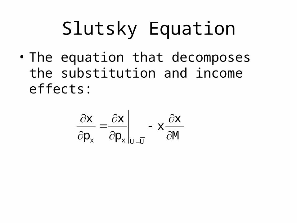
Slutsky Equation• The equation that decomposes the
substitution and income effects:
x x U U
x x xx
p p M
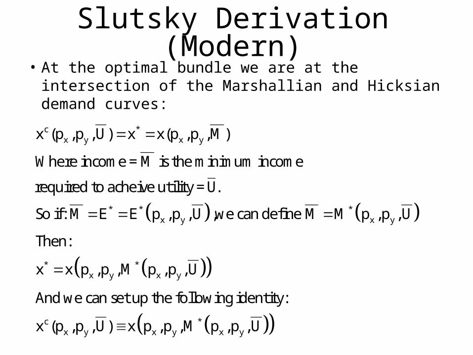
Slutsky Derivation (Modern)• At the optimal bundle we are at the intersection
of the Marshallian and Hicksian demand curves:
c *x y x y
* * *x y x y
* *x y x y
x (p ,p , U) x x(p ,p ,M)
M
.
M E E p ,p , U M M p ,p , U
x x p ,p ,M p ,p , U
Where income = is the minimum income
required to acheive utility = U
So if: ,we can define
Then:
And we can set up the following i
c *x y x y x yx (p ,p , U) x p ,p ,M p ,p , U
dentity:

Start with that identity
*
c *x y x y x y
*cx yx y x y x y
x x x
*x y x
cx
x
y
y x y x y
x x
x (p ,p , U) x p ,p ,M p ,p , U
M p ,p , Ux (p ,p , U) x(p ,p ,M) x(p ,p ,M)
p p M p
M p ,p , U
x (p ,p , U) x(p ,p ,M) x(p ,p ,
E p
p
, U
p
,p
And we can differentiate each side w.r.t. p :
And since
cx y x y x y
x
*x y
x
cx y
x
M)
M
x (p ,p , U) x(p ,p ,M) x(p ,p ,M
E p ,p , U
p
x ()
p pp , U
Mp , )
By Shepard's Lemma,
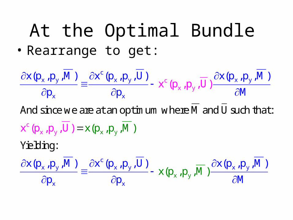
At the Optimal Bundle• Rearrange to get:
x y
x
cx y
cx y
cx y x y x
y
y
x x
cx y x y x y
x x
x(p ,p ,M) x (p ,p , U) x(p ,p ,M)
p p M
x(p ,p ,M) x (p ,p , U) x(p ,p ,M)
p
x (p ,p , U)
x (p ,p x(, U) p ,p ,M)
x(p ,p ,M)p M
And since we are at an optimum where M and U such that:
Yielding:
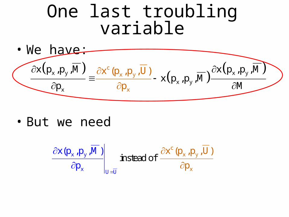
One last troubling variable
• We have:
• But we need
x yc
x y
x
x y
x yx
x (p ,p , U)x p ,p ,M x p ,p ,Mx p ,p ,M
Mpp
x y
x
cx y
xU U
instead ofxx(p ,p , (pM , U
))
p
p ,
p
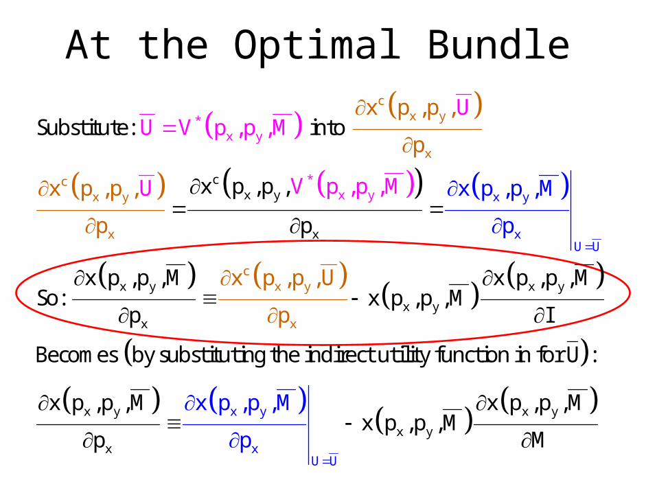
At the Optimal Bundle
cx y
x
x
x y
x
y x y
x y
cx y
x
cx y
x
cx y
x
*x
U U
y
*x y
x
x p ,p ,
p
x p ,p ,M x p ,p ,Mx p ,p ,M
x p ,p ,
p
x p ,p ,
UU V p ,p ,M
V p
p
x p ,p , U
x p ,p ,M
p
p
p
M
p
,U
I
,
Substitute: into
So:
Becomes by substituting the indirect utility function in
x y x y
x yx
x y
xU U
x p ,p ,Mx p ,p ,M x p ,p ,Mx p ,p ,M
p Mp
for U :
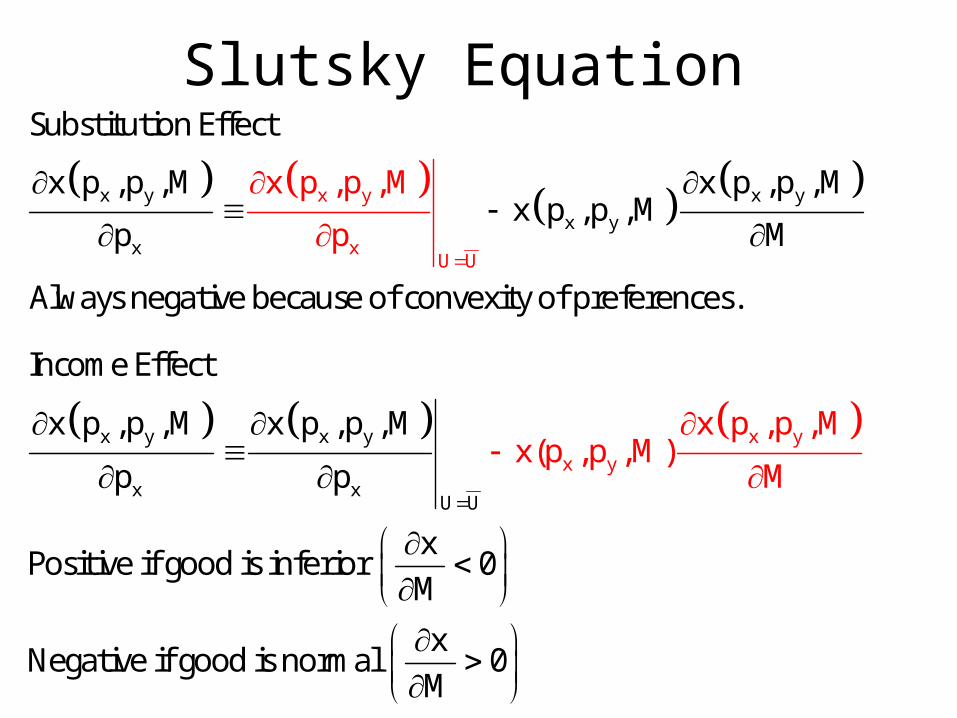
Slutsky Equation
x y xx y
x
y
x yx
U U
x p ,p ,M x p ,px p ,p ,M ,Mx p ,p ,M
pp M
Substitution Effect
Always negative because of convexity of preferences.
x y
x
x y x y
xU
yx
U
x p ,p ,Mx(p ,p ,M
x p ,p)
,M x p ,p ,M
p p
x0
M
x0
M
M
Income Effect
Positive if good is inferior
Negative if good is normal
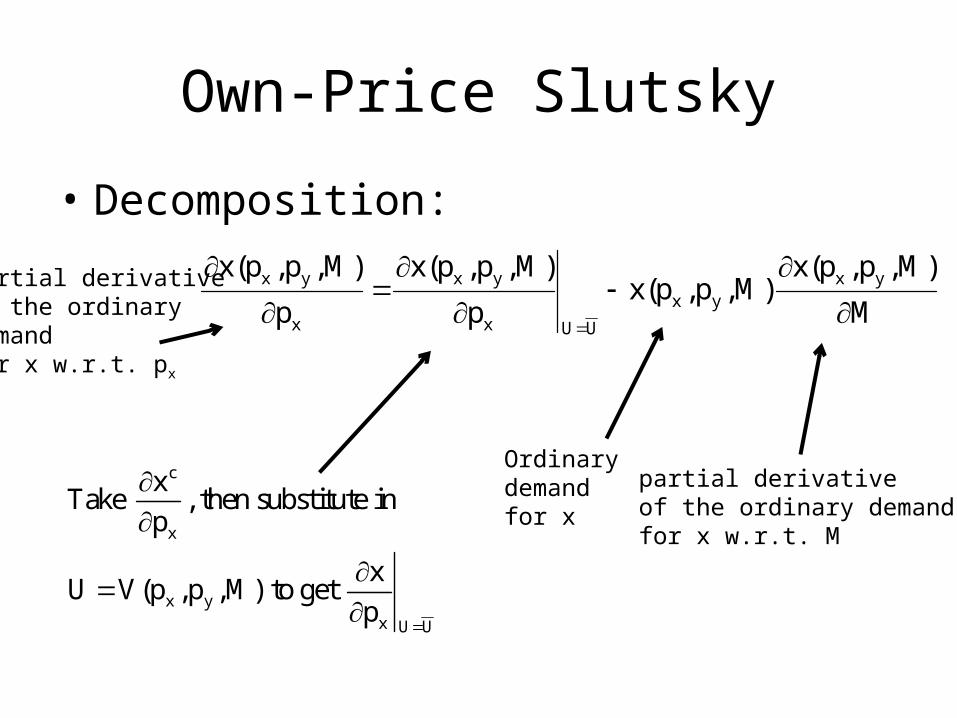
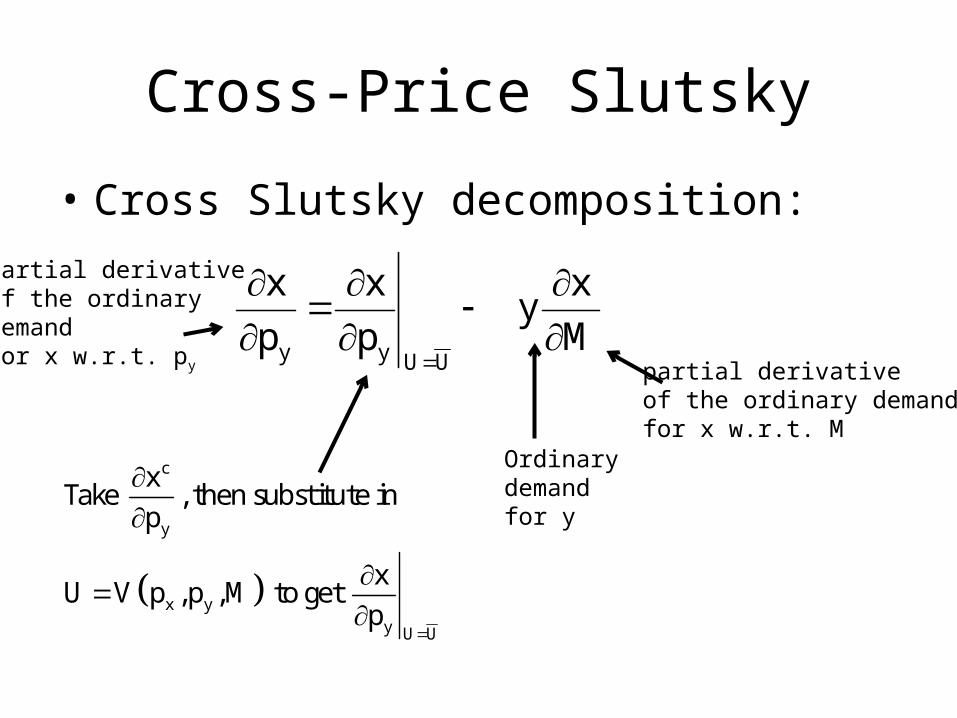
Own-Price Slutsky
• Decomposition:
x y x y x yx y
x x U U
x(p ,p ,M) x(p ,p ,M) x(p ,p ,M)x(p ,p ,M)
p p M
c
x
x yx U U
xTake , then substitute in
p
xU V(p ,p ,M) to get
p
Ordinary demand for x partial derivative
of the ordinary demand for x w.r.t. M
partial derivativeof the ordinarydemand for x w.r.t. px
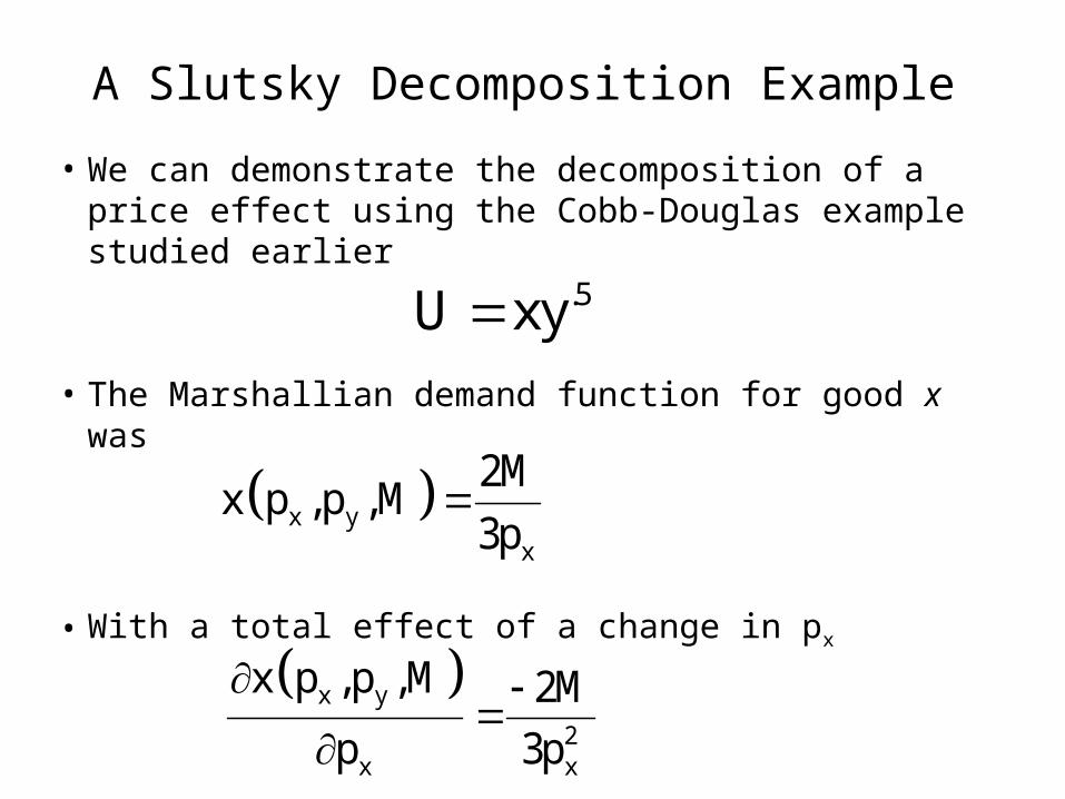
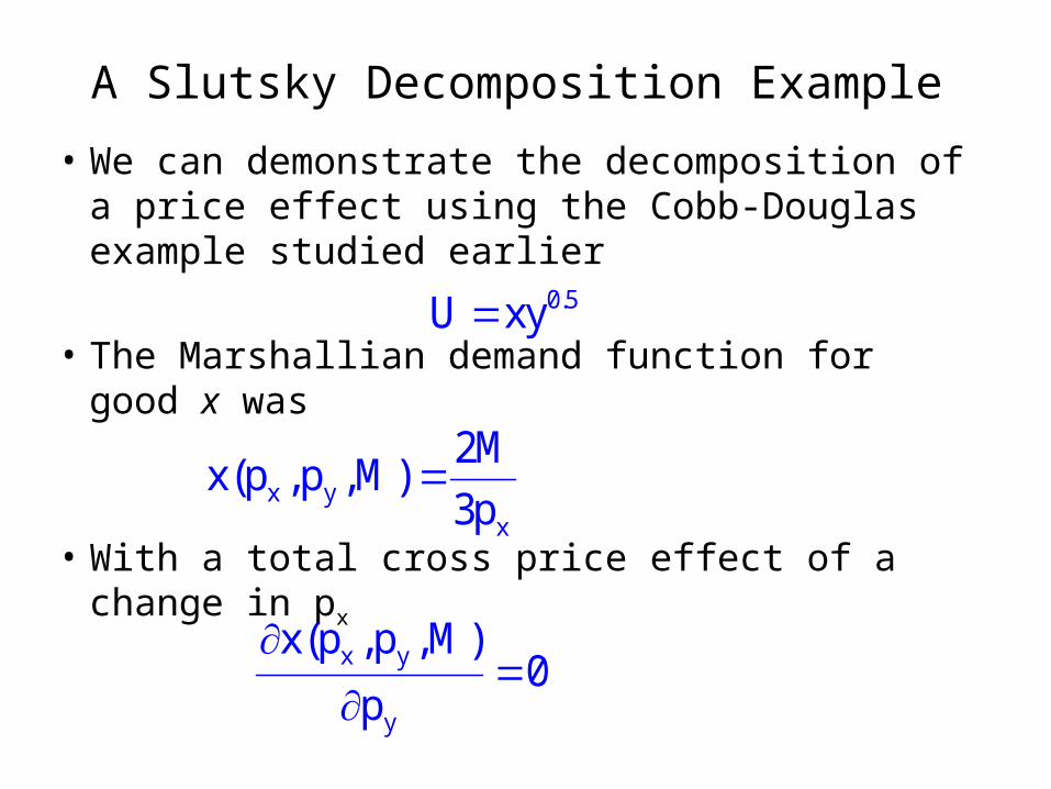
A Slutsky Decomposition Example• We can demonstrate the decomposition of a price
effect using the Cobb-Douglas example studied earlier
• The Marshallian demand function for good x was
• With a total effect of a change in px
x yx
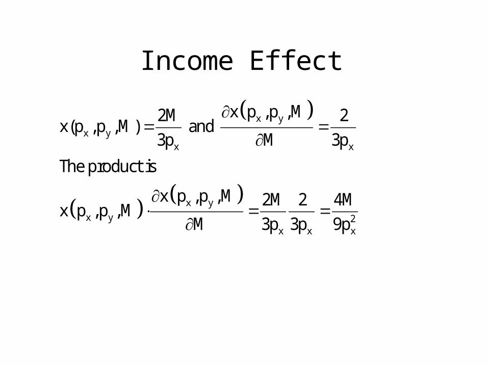
2Mx p ,p ,M
3p
x y
2x x
x p ,p ,M 2M
p 3p
.5U xy
43
1/3 1/32/3 c 2/3y x y yc
x y 1/3 4/3x x x
x
32
12
x y
y
2/3
1/3
y
x y
2U U
32
12
x y
x xx
U 2p x p ,p , U 2px p ,p , U
p
U
2MU
3
p 3p
V p ,p ,M
2px p ,p ,M 2M
p 9p3p
p 3p
2M
3p 3p
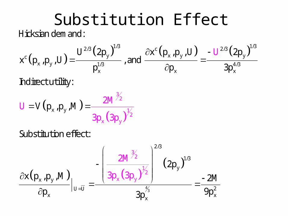
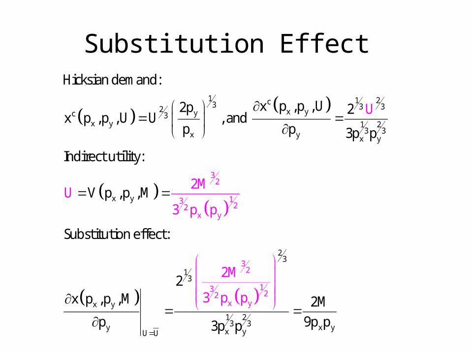
Hicksian demand:
, and
Indirect utility:
Substitution effect:
Substitution Effect
x y
x yx x
x y
x y 2x x x
x p ,p ,M2M 2x(p ,p ,M)
3p M 3p
x p ,p ,M 2M 2 4Mx p ,p ,M
M 3p 3p 9p
and
The product is
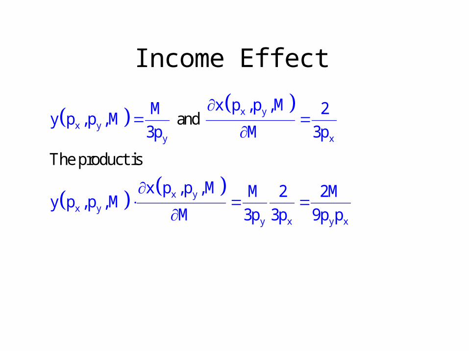
Income Effect
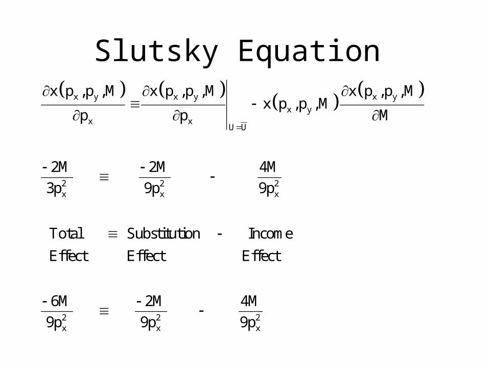
Slutsky Equation x y x y x y
x yx x
U U
2 2 2x x x
x p ,p ,M x p ,p ,M x p ,p ,Mx p ,p ,M
p p M
2M 2M 4M
3p 9p 9p
Total Substitution Income
Effect Effect Effe
2 2 2x x x
ct
6M 2M 4M
9p 9p 9p
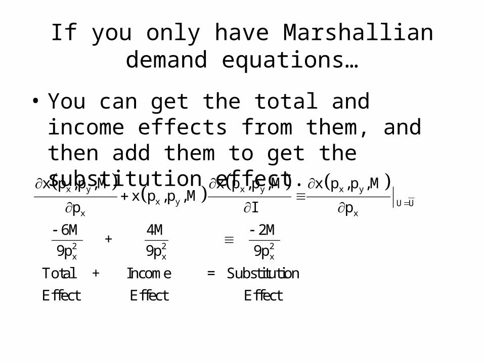
If you only have Marshallian demand equations…
• You can get the total and income effects from them, and then add them to get the substitution effect. x y x y x y
x y U Ux x
2 2 2x x x
x p ,p ,M x p ,p ,M x p ,p ,Mx p ,p ,M
p I p
6M 4M 2M +
9p 9p 9p
Total + Income = Substitution
Effect Effect
Effect
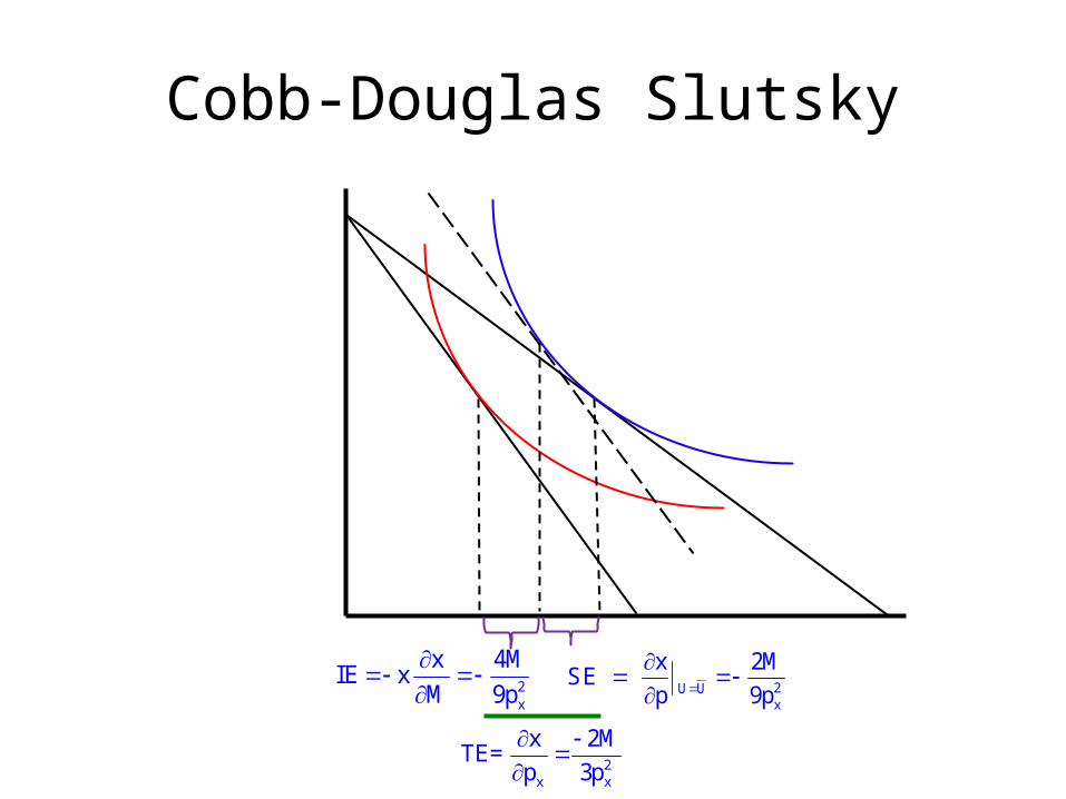
Cobb-Douglas Slutsky
2x
x 4Mx
M 9p
IE
2U Ux
x 2M
p 9p
SE
2x x
x 2M
p 3p
TE=
Cross Price Effects,
• Out analysis of cross-price effects in a two-good world is limited as spending more on x, necessarily means spending less on y and vice-versa.
• Yet, we can use the two good world to define terms and gain an intuitive understanding.
y
x
p
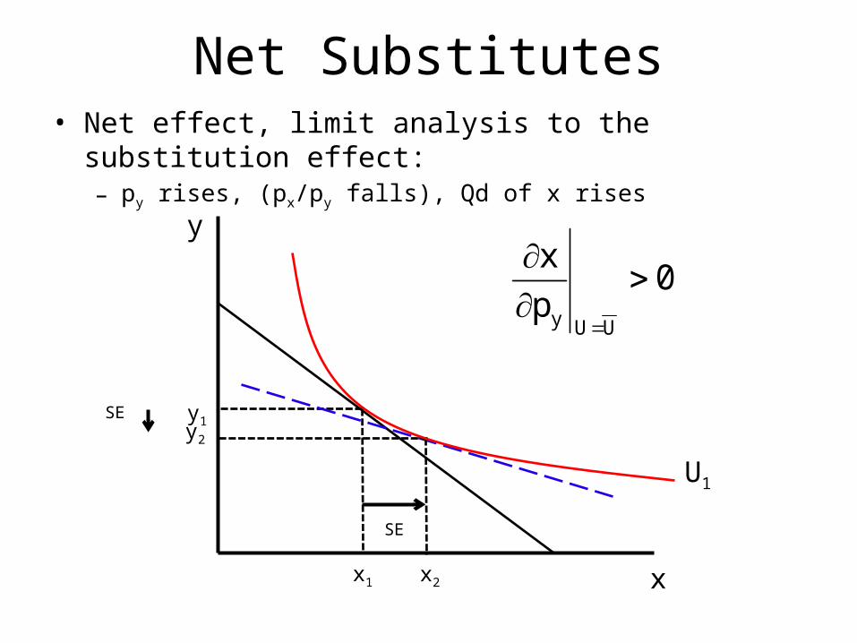
Net Substitutes• Net effect, limit analysis to the substitution effect:
– py rises, (px/py falls), Qd of x rises
y
x1 xx2
y2
y1
U1
SE
y U U
x0
p
SE
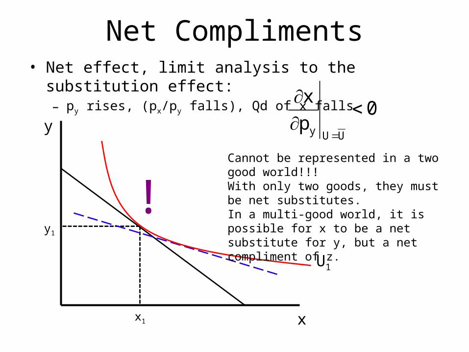
Net Compliments• Net effect, limit analysis to the substitution effect:
– py rises, (px/py falls), Qd of x falls
y
x1 x
y1
U1
y U U
x0
p
Cannot be represented in a two good world!!!With only two goods, they must be net substitutes.In a multi-good world, it is possible for x to be a net substitute for y, but a net compliment of z.!
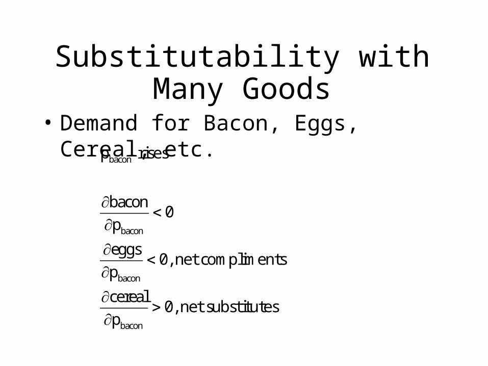
Substitutability with Many Goods
• Demand for Bacon, Eggs, Cereal, etc.bacon
bacon
bacon
bacon
p
bacon0
p
eggs0
p
cereal0
p
rises
, net compliments
, net substitutes
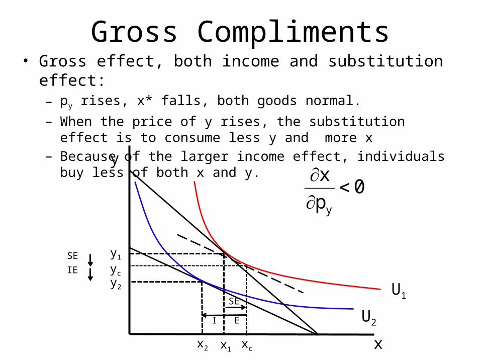
Gross Compliments• Gross effect, both income and substitution effect:
– py rises, x* falls, both goods normal.– When the price of y rises, the substitution effect is to consume less y and
more x– Because of the larger income effect, individuals buy less of both x and y.
y
x1 xx2
y2
y1
U1
U2
SE
I E
SE
IE yc
xc
y
x0
p
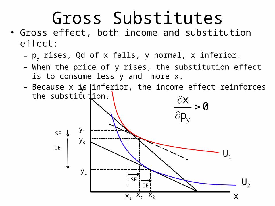
Gross Substitutes• Gross effect, both income and substitution effect:
– py rises, Qd of x falls, y normal, x inferior.– When the price of y rises, the substitution effect is to consume less y and
more x.– Because x is inferior, the income effect reinforces the substitution.
y
x1 xx2
y2
y1
U1
U2SE
IE
SE
IE
yc
xc
y
x0
p
Gross Effects
• Is the status (normal vs. inferior) the determining feature?
• No. You can have gross substitutes even if x is inferior, so long as the income effect is small.
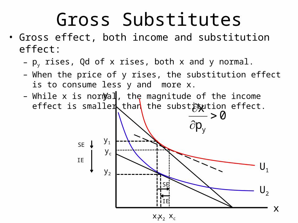
Gross Substitutes• Gross effect, both income and substitution effect:
– py rises, Qd of x rises, both x and y normal.– When the price of y rises, the substitution effect is to consume less y and
more x.– While x is normal, the magnitude of the income effect is smaller than the
substitution effect. y
x1
xx2
y2
y1
U1
U2
SE
IE
SE
IE
yc
xc
y
x0
p
Asymmetry of the Gross Definitions
• The gross definitions of substitutes and complements are not symmetric– it is possible for x to be a gross substitute for y
(when the price of y changes) and at the same time for y to be a gross complement of x (when the price of x changes).
Asymmetry of the Gross Definitions
• Suppose that the utility function for two goods is given by
U(x,y) = ln x + y
• Setting up the Lagrangian
L = ln x + y + (M – pxx – pyy)
Asymmetry of the Gross Definitions
• We get the following FOCs:
Lx = 1/x - px = 0
Ly = 1 - py = 0
Lλ = M - pxx - pyy = 0
• Manipulating the first two equations, we getpxx = py
Asymmetry of the Gross Definitions
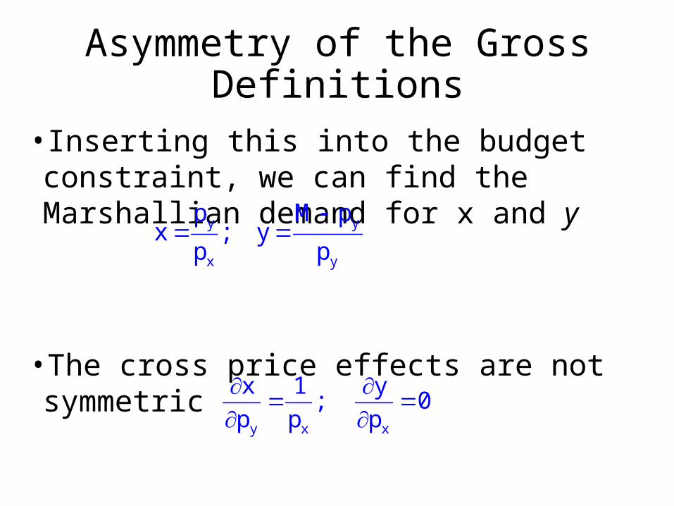
• Inserting this into the budget constraint, we can find the Marshallian demand for x and y
•The cross price effects are not symmetric
y y
x y
p M px y
p p
;
y x x
x 1 y0
p p p;
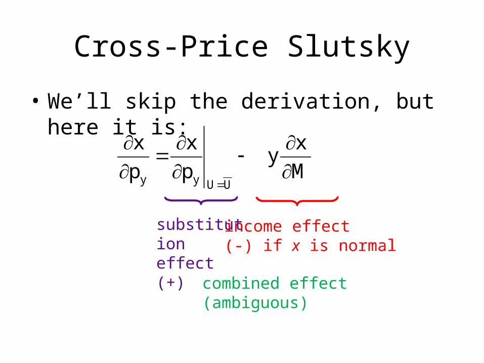
Cross-Price Slutsky
• We’ll skip the derivation, but here it is:
y y U U
x x xy
p p M
income effect(-) if x is normal
combined effect(ambiguous)
substitutioneffect (+)
Cross-Price Slutsky
• Cross Slutsky decomposition:
y y U U
x x xy
p p M
c
y
x yy U U
x
p
xU V p ,p ,M
p
Take , then substitute in
to get
Ordinary demand for y
partial derivativeof the ordinary demand for x w.r.t. M
partial derivativeof the ordinarydemand for x w.r.t. py
A Slutsky Decomposition Example• We can demonstrate the decomposition of a
price effect using the Cobb-Douglas example studied earlier
• The Marshallian demand function for good x was
• With a total cross price effect of a change in px
x yx
2Mx(p ,p ,M)
3p
x y
y
x(p ,p ,M)0
p
0.5U xy
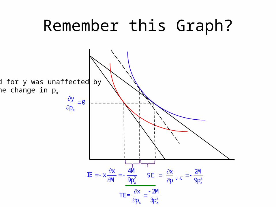
Remember this Graph?
x
y0
p
Qd for y was unaffected bythe change in px
2x
x 4Mx
M 9p
IE
2U Ux
x 2M
p 9p
SE
2x x
x 2M
p 3p
TE=
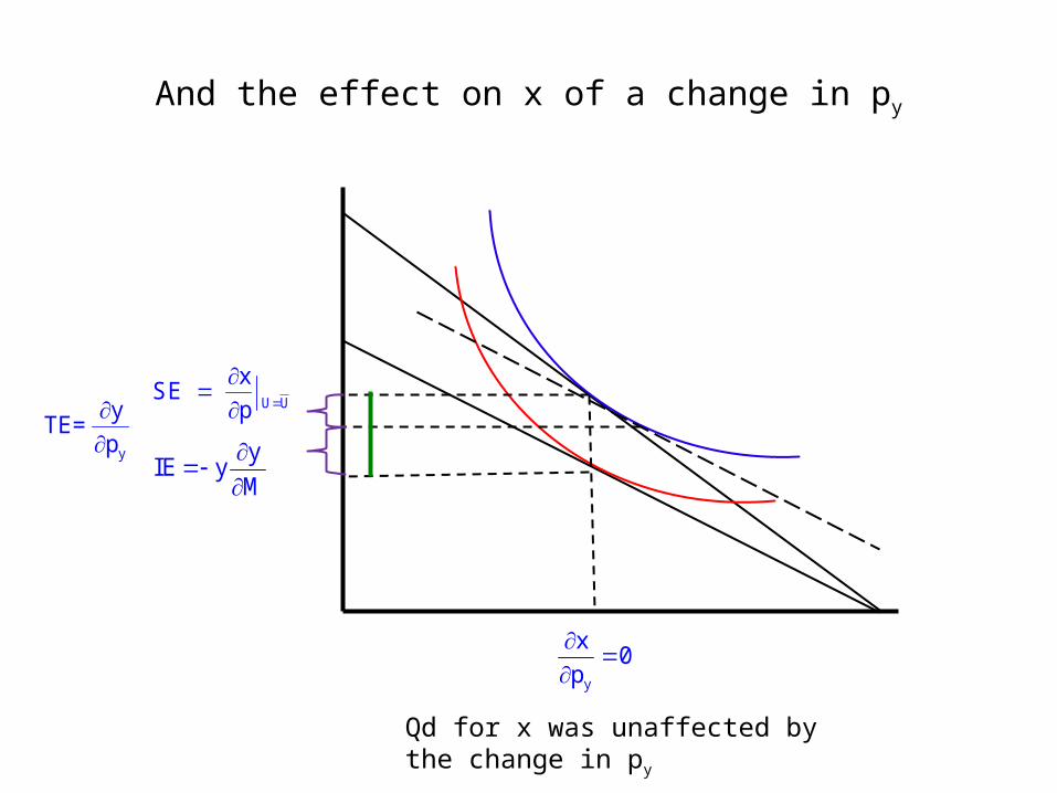
And the effect on x of a change in py
y
x0
p
Qd for x was unaffected bythe change in py
yy
M
IE
U U
x
p
SE
y
y
p
TE=
1 1 2c3 3 32 x yyc 3x y 1 2
3 3x y x y
x y
23
13
x y
32
1322
x
1 23 3y x yx
y
32
1
U
2
yU
32
x y
x p ,p , U2p 2x p ,p , U U
p p 3p p
V p ,p ,M
2x p ,p
U
2MU
3 p p
2M
3 p,M 2M
p 9p p3p p
p
Hicksian demand:
, and
Indirect utility:
Substitution effect:
Substitution Effect
x y
x yy x
x y
x yy x y x
and
The produ
x p ,p ,MM 2y p ,p ,M
3p M 3p
x p ,p ,M M 2 2My p ,p ,M
M 3p
ct
3p 9p p
is
Income Effect
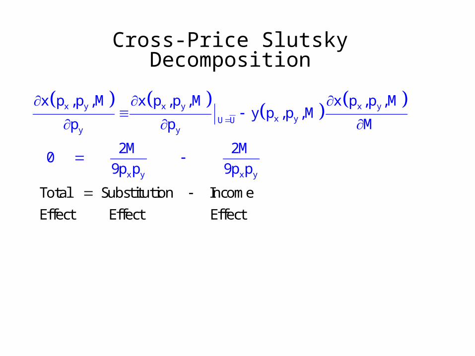
Cross-Price Slutsky Decomposition
x y x y x y
x yU Uy y
x y x y
x p ,p ,M x p ,p ,M x p ,p ,My p ,p ,M
p p M
2M 2M0
9p p 9p p
Total Substitution Income Effe
ct Effect
Effe
ct
Slutsky Equation Via Comparative Statics
• Using Utility Maximization and Expenditure Minimization
• Yes, Rockin’ it Old School
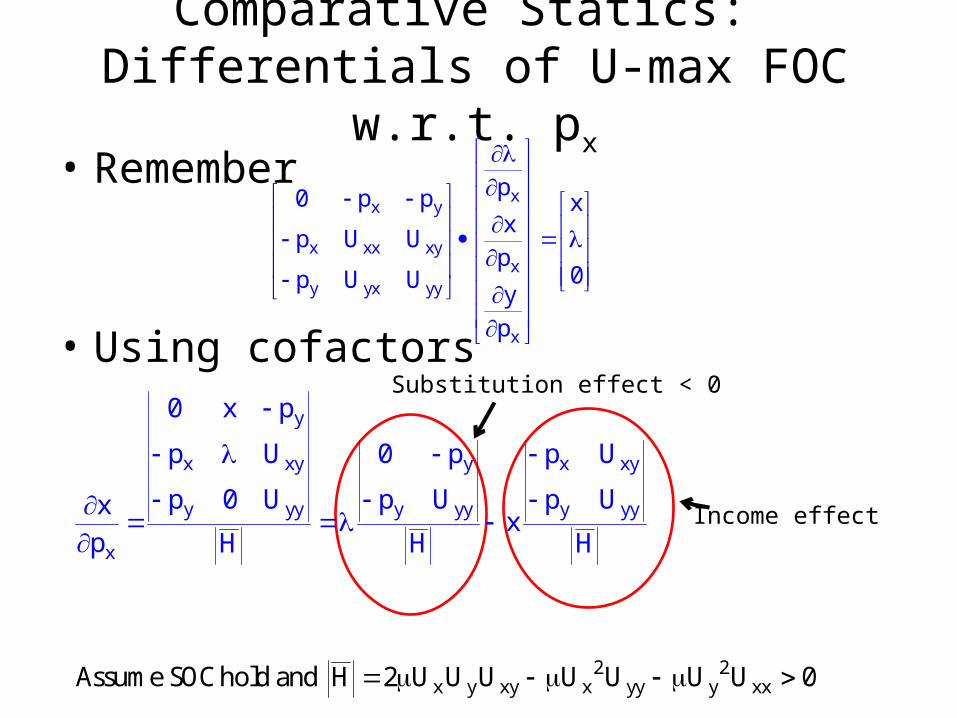
Comparative Statics: Differentials of U-max FOC w.r.t. px
• Remember
• Using cofactors
xx y
x xx xyx
y yx yy
x
p0 p p xx
p U Up
0p U Uy
p
y
x xy y x xy
y yy y yy y y
2 2x y xy x yy
y
x
y xx
0 x p
p U 0 p p
H 2 U U U U U U U
U
p
0
0 U p U p Uxx
p H H H
Assume SOC hold and
Substitution effect < 0
Income effect
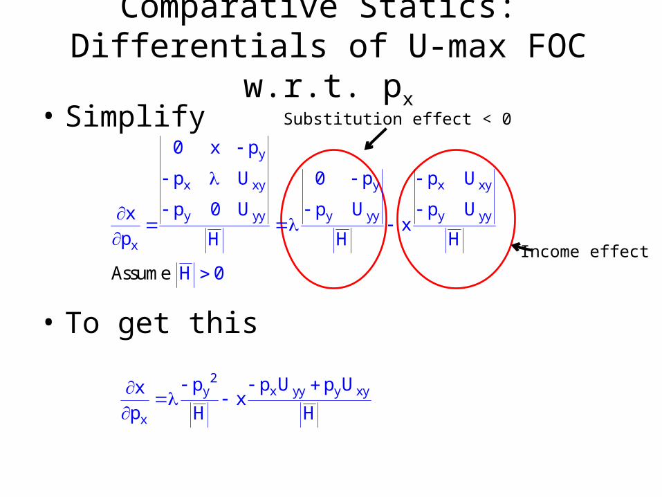
Comparative Statics: Differentials of U-max FOC w.r.t. px
• Simplify
• To get this
y
x xy y x xy
y yy y yy y yy
x
0 x p
p U 0 p p U
p 0 U p U p Uxx
p H H H
H 0Assume
Substitution effect < 0
Income effect
2y x yy y xy
x
p p U p Uxx
p H H
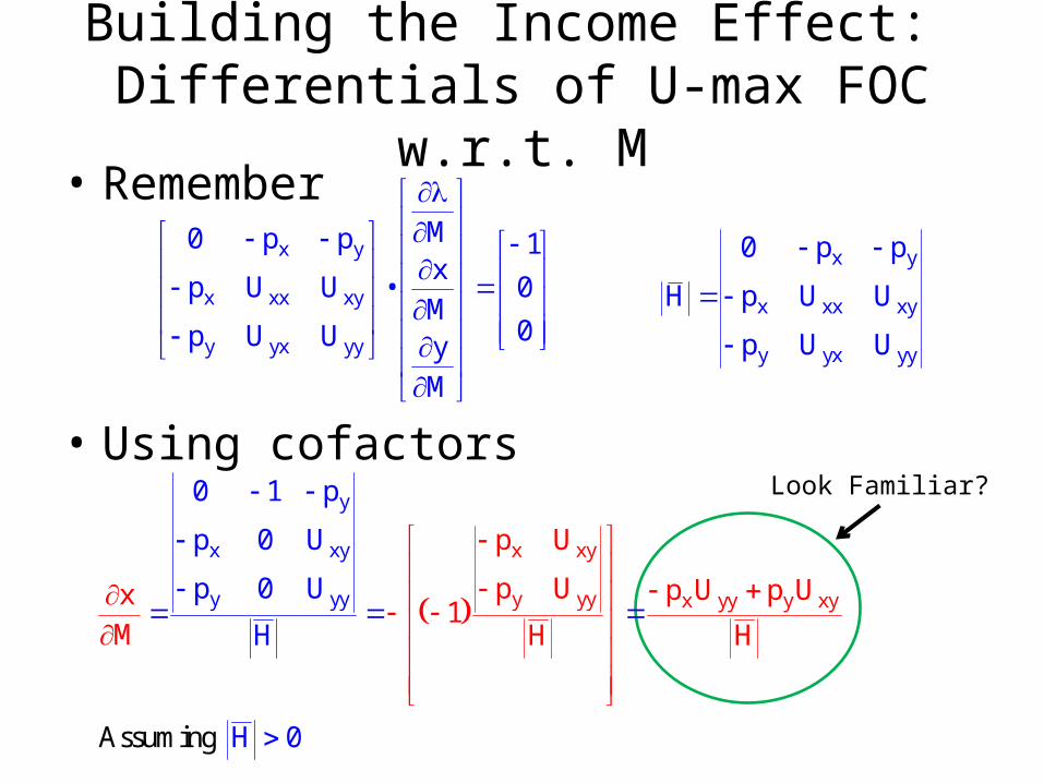
Building the Income Effect: Differentials of U-max FOC w.r.t. M
• Remember
• Using cofactors
x y
x xx xy
y yx yy
M0 p p 1x
p U U • 0M
0p U U y
M
x xy
y yy x
y
x xy
y y yy yy xy
p U
p U p U p Ux1
M H
0 1
Assuming
p
p 0 U
p 0 U
H 0
HH
Look Familiar?
x y
x xx xy
y yx yy
0 p p
H p U U
p U U
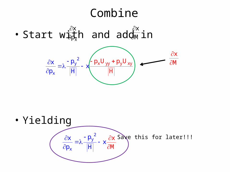
Combine
• Start with and add in
• Yielding
x
M
x
x
p
x
M
2y
x
pxx
p H
x
M
Save this for later!!!
x yy y
x
xy2
ypxx
p U U
HH
p
p
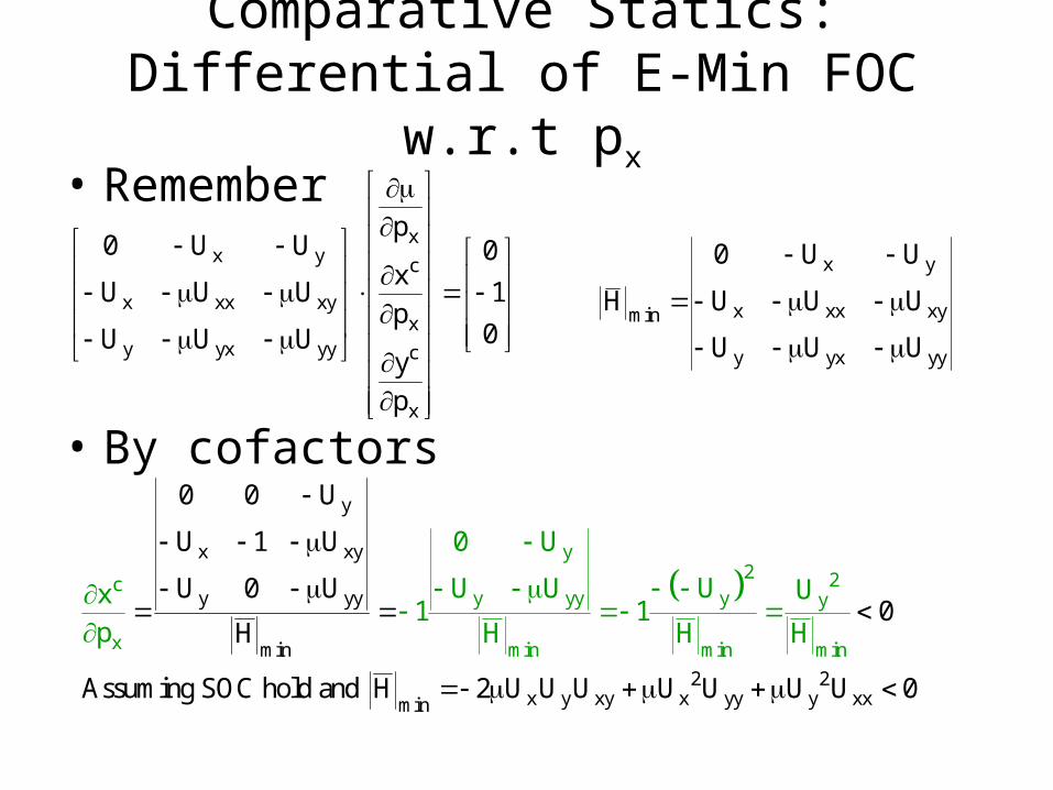
Comparative Statics:Differential of E-Min FOC w.r.t px
• Remember
• By cofactors
xx y c
x xx xyx
y yx yy c
x
p0 U U 0
xU U U 1
p0U U U
y
p
y
2 2cyy yy y
x min min min
y
x xy
y yy
min
2 2x y xy x yy y xxmin
0 0 U
U 1 U
U 0 U0
H
Assuming SOC hold
0 U
UU
an
U Ux
d H
1 1p H H
2 U U U U 0
H
U U U
x y
x xx xymin
y yx yy
0 U U
H U U U
U U U
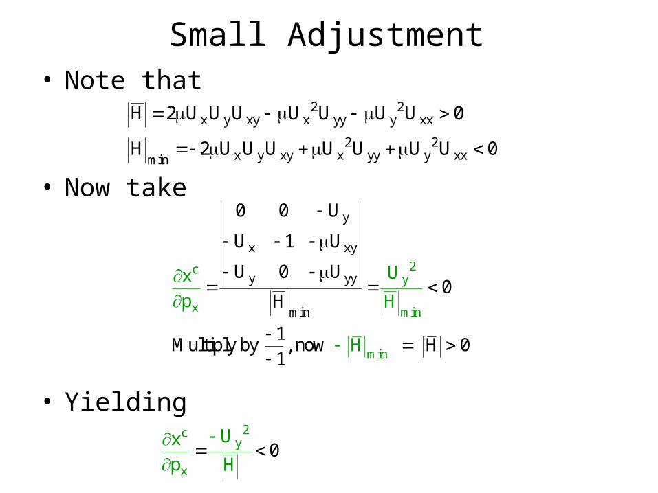
Small Adjustment• Note that
• Now take
• Yielding2c
y
x
Ux
p H0
2 2x y xy x yy y xx
2 2x y xy x yy y xxmin
H 2 U U U U U U U 0
H 2 U U U U U U U 0
y
2
x xy
yc
yy
x min
min
y
min
Ux
p H
0 0 U
U 1 U
U 0 U0
H
1Multiply by , now H 0
1H
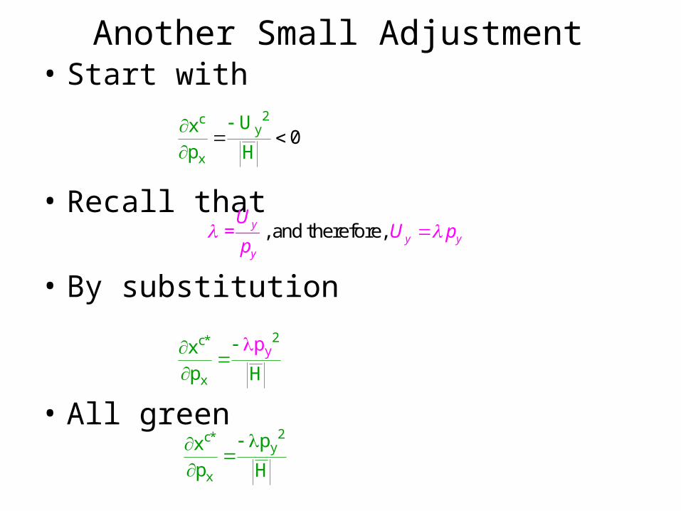
Another Small Adjustment• Start with
• Recall that
• By substitution
• All green
, and therefore, = yy y
y
UU p
p
2c*y
x
px
p H
2cy
x
Ux
p H0
x
y2c*x
p
p
H
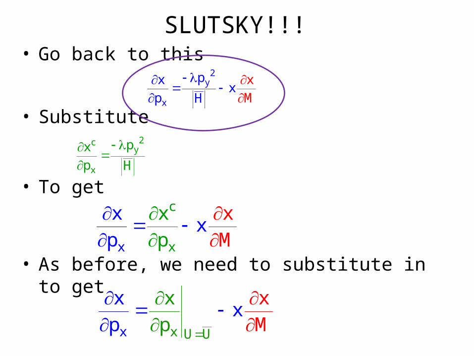
SLUTSKY!!!• Go back to this
• Substitute
• To get
• As before, we need to substitute in to get x
c
x
x
p M
x
p
xx
2y
x
pxx
p H
x
M
2cy
x
px
p H
x U Ux
xx
M
x x
pp