income elasticities of food demand in africa: a meta-analysis · and external country-level factors...
TRANSCRIPT
Patricia C. Melo
Yakubu Abdul-Salam
Deborah Roberts
Alana Gilbert
Robin Matthews
Liesbeth Colen
Sébastien Mary
Sergio Gomez Y Paloma
Income Elasticities of Food Demand in Africa: A Meta-Analysis
2015
EUR 27650 EN
Income Elasticities of Food Demand in Africa: A Meta-Analysis
Patricia C. Melo1
Yakubu Abdul-Salam1
Deborah Roberts1
Alana Gilbert1
Robin Matthews1
Liesbeth Colen2
Sébastien Mary3
Sergio Gomez Y Paloma2
1 James Hutton Institute, UK
2 European Commission, JRC-IPTS, Seville, Spain
3 DePaul University, Driehaus College of Business, Chicago, US
This publication is a Technical report by the Joint Research Centre, the European Commission’s in-house science
service. It aims to provide evidence-based scientific support to the European policy-making process. The scientific
output expressed does not imply a policy position of the European Commission. Neither the European
Commission nor any person acting on behalf of the Commission is responsible for the use which might be made
of this publication.
JRC Science Hub
https://ec.europa.eu/jrc
JRC98812
EUR 27650 EN
ISBN 978-92-79-54182-7
ISSN 1831-9424 (online)
doi:10.2791/661366 (online)
© European Union, 2015
Reproduction is authorised provided the source is acknowledged.
All images © European Union 2015, except: Cover images, fresnel6 (left), Mariusz Prusaczyk (middle), Loulou &
Lily (right), Fotolia.com.
How to cite: Melo, P., Abdul-Salam, Y., Roberts, D., Gilbert, A., Matthews, R., Colen, L., Mary, S., Gomez Y
Paloma, S.; Income Elasticities of Food Demand in Africa: A Meta-Analysis; EUR 27650 EN; doi:10.2791/661366
Table of contents
Executive Summary ....................................................................................................... 5
1. Introduction ........................................................................................................... 7
1.1 Food demand and income ...................................................................................... 7
1.2 Aims and objectives .............................................................................................. 8
2. Research Methods ................................................................................................. 11
2.1 Development of the meta-sample ....................................................................... 11
2.1.1 Search terms and selection strategy .............................................................. 11
2.1.2 Data extraction ........................................................................................... 12
2.1.3 External variables ....................................................................................... 12
2.2 Meta-regression analysis ................................................................................... 16
2.2.1 Specification of the meta-regression model .................................................... 16
2.2.2 Potential estimation issues in the meta-regression model and sensitivity analysis 17
2.2.3 Sensitivity testing ....................................................................................... 17
3. Description of the meta-sample .............................................................................. 19
3.1 Studies included in the meta-sample .................................................................. 19
3.2 Sample size and distribution by study ................................................................. 19
3.3 Type of publication ........................................................................................... 21
3.4 Type of food demand ........................................................................................ 21
3.5 Food groups .................................................................................................... 22
3.6 Nutrients ......................................................................................................... 24
3.7 Regions ........................................................................................................... 24
3.8 Urban versus rural location and degree of urbanisation ......................................... 25
3.9 Household income segment and diet ................................................................... 26
3.10 Country income level ...................................................................................... 27
3.11 Time period ................................................................................................... 28
3.12 Journal ranking .............................................................................................. 28
4 Meta-Regression Analyses ....................................................................................... 30
4.1 Estimation issues ............................................................................................. 30
4.2 Foods .............................................................................................................. 32
4.2.1 All foods .................................................................................................... 32
4.2.2 Results by food types .................................................................................. 35
5. Sensitivity Analysis ............................................................................................... 51
5.1 Sample-size weighted meta-regressions .............................................................. 51
5.2 Publication bias and journal ranking .................................................................... 53
5.2 Additional control variables ................................................................................ 56
6. Conclusion ........................................................................................................... 57
7. References ........................................................................................................... 59

Appendix ................................................................................................................. 61
A.1. List of studies included in the meta-sample ........................................................ 61
A.2. List of studies identified but subsequently not included in the meta-sample ............ 64
A.3. Results from the regression analyses by food type .............................................. 66
List of figures ................................................................................................................ 1
List of tables ................................................................................................................. 2

Acknowledgements
The authors would like to thank Pierre Fabre, Pierpaolo Piras and Lucia Fernandez Castillo for
their support and comments to the report.
Executive Summary
Food demand in Sub-Saharan Africa is rapidly changing. Given an expanding population, rising
incomes and intensified urbanization, the demand for food will not only continue to rise, but
will also change in its composition. In order to combat malnutrition, economists and
policymakers need to understand better, first, the factors underlying the relation between
income and food demand, and, second, how this relation is changing according to the income
level and/or characteristics of the country under study. Such understanding will help to
improve the design and implementation of nutrition policies as the continent further develops.
There are a number of studies that have estimated the relation between income growth and
food demand in Africa, but the resulting estimates are highly heterogeneous. This report
provides a systematic review of the existing literature on income elasticities of food demand in
Africa. A meta-sample has been constructed including both attributes of the primary studies
and external country-level factors thought to influence the income elasticities.
The sample includes elasticities for different categories of food (cereals, legumes and nuts,
meat, fish and eggs, dairy products, fruits and vegetables, and beverages) as well as
elasticities for calorie and nutrient consumption. A total of 2,101 elasticity estimates drawn
from 66 studies and covering 54 African countries have been included in the sample.
Descriptive statistics indicate that food demand is more responsive to changes in income (in
other words, income elasticities are higher) for beverages, meat, fish and eggs and dairy,
compared to foods that tend to constitute basic diets (e.g. cereals, legumes and nuts, fruit and
vegetables, and fats and oils, tubers). Correspondingly, certain nutrient elasticities (especially
elasticities of demand for proteins) are found to be higher than calorie elasticities.
Based on this sample, meta-regression analyses were conducted for each of the food
categories separately, as well as for food, calorie and nutrient demand as a whole. The role of
methodological factors and country-level characteristics in explaining the different responses of
food demand to income have been examined. There is no strong evidence of major
methodological and data-related differences, although some tendencies can be identified: the
use of panel data, the use of expenditures as a proxy for income and the use of single-
equation models rather than demand systems all seem to result in lower elasticities.
Factors relating to a country’s income and degree of urbanisation, time period of primary data,
and geographical sub-region (e.g. Western Africa) are found to explain heterogeneity in the
estimated elasticities. For calorie demand and food demand in general, we find that a higher
level of income results in lower elasticities. For nutrient demand, we find instead that
elasticities are higher in richer countries. This suggests that as countries grow richer,
households tend to spend more on food with higher nutritional value. We also find that for
most types of food, elasticities tend to be lower in urban areas or in countries with a larger
share of urban population.
The considerable regional differences in food-income elasticities across African sub-regions
suggest that the impact of agricultural and nutrition policies may be expected to differ by
region. Further research could usefully explore in greater detail some of the patterns identified
and, in doing so, contribute to the design of policies aimed at addressing malnutrition.
1. Introduction
Ensuring food security in Sub-Saharan Africa (SSA) remains a huge challenge, and will
continue to be so in the coming decades. FAO, IFAD and WFP (2015) estimate that over 200
million people in Africa are hungry. The share of undernourished people in SSA has declined
(from 27.6% in 1990-1992 to 20.7% in 2010-2012), but at a considerably slower pace than in
the rest of the developing world. Moreover, given that by 2050 the population of SSA is
expected to double (UNPD, 2015), feeding the poor will remain an enormous challenge. Not
only will the demand for food continue to rise, but also the composition of food demand will
change with rising incomes and growing urbanization contributing to changing diets (Popkin,
1994). With more than half of the African population projected to live in cities by 2050 and
average growth of GDP in SSA continuing at a rate of 4 to 5 percent in the coming years
(World Bank, 2015), the composition of African food demand may be expected to alter
substantially in the future.
Beyond these general trends, studies note that there are significant differences in dietary
patterns and food supply structures across regions (Fabiosa, 2011). These differences
influence the relationship between income and food demand and thus the impact of alternative
policy mechanisms in different areas. An examination of the drivers of food demand, and how
they are changing over time especially in the face of growing national incomes, is needed to
reveal the impact of growth and policy interventions on malnutrition. For example, a large
responsiveness of food demand to rising incomes suggests that income-oriented policy
interventions can be an effective tool to combat undernutrition, while a low responsiveness
indicates that income growth will affect food demand only to a limited extent and that other
types of policy interventions will be needed. Also, for projecting future patterns of food
demand, it is important to know how demand will respond to rising incomes and which
segments of the population will be most threatened by hunger. Overall, a better understanding
of food demand is needed to inform policies aimed at improving food security across Africa.
1.1 Food demand and income
Generally, the income elasticity of food demand (i.e. the percentage change in food
consumption in response to a 1% change in income) is positive but smaller than 1, i.e.
spending on food increases less than proportionally with total expenditures. For poor people,
food makes up an important share of household spending. However, as people get richer, they
tend to allocate proportionally more of that additional income to non-food items, reducing the
share they spend on food. As a result, even though total spending on food increases, the share
of total income devoted to food declines, also known as Engel’s Law. This also explains why, as
people become richer and their daily calorie demand is fulfilled, they start spending more on
the taste, quality and diversity of their food instead of the amount of food (Jensen and Miller,
2011), i.e. the “trading up” of food consumption. As a result, the composition of people’s food
basket is changing Understanding the relationship between income and the demand for food is
critical for the design of policies aimed at addressing under-nutrition and improving food
security in developing countries. Studies which have looked at the relationship at global level
have found evidence of “trading up” (whereby consumption patterns shift as income levels
increase towards high value protein rich meat and dairy products, more convenience foods and
specific product characteristics) and “convergence” (whereby the consumption patterns in low
to middle income countries converge, over time, towards the consumption patterns in high
income countries). However, studies also note that there are significant differences in dietary
patterns and food supply structures both across regions and within regions such as Africa
(Fabiosa, 2011). These differences influence the relationship between income and food
demand and thus the impact of alternative policy mechanisms in different areas.
By and large, the existing literature on income and food demand has focused on the
relationship between income and calorie consumption (i.e. calorie-income elasticities), while
relatively few have considered the nutrient composition (e.g. fats, proteins, carbohydrates) of
calorie consumption (see Salois et al., 2012). Studies have shown that the relationship
between income and calorie consumption is not linear and that the increase in the demand for
calories as a result of income growth becomes smaller as income levels become higher (i.e. the
income elasticity of demand is less elastic for higher income countries or groups of the
population with higher income). This is thought to result from the reaching of a saturation
point in calorie consumption (e.g. Skoufias et al., 2011, Salois et al., 2012) and the preference
for higher quality foods with increased income, without changing their nutrient composition
(e.g. Jensen and Miller, 2011, Skoufias et al., 2011).
1.2 Aims and objectives
A large number of studies have estimated the relation between food demand and income for
specific categories of food, time periods and countries. Yet, the resulting elasticity estimates
vary widely across studies. In this report we examine the relation between income and food,
calorie and nutrient consumption through a systematic review of the existing literature,
specifically focusing on Africa. Through a meta-analysis approach, we aim to explain this large
heterogeneity in income elasticities across the African continent in terms of country attributes,
the specific food or nutrient categories considered, or the methodological characteristics of the
data and estimation techniques. Meta-analysis provides an objective approach to review
empirical literature through the use of statistical techniques (Stanley and Jarrell, 2005)1. As
such, our main objectives are to identify the factors underlying differences in the estimated
food income elasticities within and between developing countries in Africa.
The report draws on recent review studies, including other meta-analyses of food demand
(e.g. Bouis and Haddad, 1992, Salois et al., 2012, Ogundari and Abdulai, 2013, Zhou and Yu,
2014)2. Table 1 provides a summary of the main features of previous review studies of calorie-
income elasticities. Yet, we extend the work in a number of ways.
First, our main interest is to uncover the explanations behind the different food income
elasticities found in the literature. While Ogundari and Abdulai (2013) did a detailed meta-
analysis of calorie-income elasticities, they focused only on the methodological explanations for
the heterogeneity in estimated elasticities. Instead, Zhou and Yu (2014) and Salois et al.
(2012) focused specifically on income to explain different elasticity estimates. Salois et al.
(2012) investigated the nature of the relationship between income and calorie and nutrient
consumption using both parametric and non-parametric methods that can accommodate
nonlinearities and make fewer (or no) assumptions about the functional form of the
relationship. Zhou and Yu (2014) discussed in detail how the calorie-income relation differs
between the ‘poor stage’ and the ‘affluent stage’. In addition to the income level, in this report,
we also explore how other country-specific factors (such as urbanization and geography) may
explain the heterogeneity in food-income elasticities across countries, while still controlling in
detail for methodological aspects of the studies.
1This approach to conducting a literature review has been more commonly applied in psychology and the medical
sciences, but has recently also gained popularity in environmental economics (e.g. Nelson and Kennedy, 2009), labour economics (e.g. Ashenfelter et al., 1999, Longhi et al., 2005, Nijkamp and Poot, 2005, Weichselbaumer and Winter-Ebmer, 2005), international economics (e.g. Rose and Stanley, 2005, de Groot et al., 2005, Disdier and Head, 2008)
and urban and regional economics (e.g. Beaudry and Schiffauerova, 2009, Melo et al. 2009, de Groot et al., 2009, Melo et al., 2013). 2Meta-analyses of price elasticities of food demand have been carried out by Andreyeva et al. (2010) and Green et al.
(2013) but are not further discussed here.

Table 1. Previous review studies of calorie-income elasticities
Study
Bouis and
Haddad
(1992) 1
Salois et al.
(2012)1
Ogundari and
Abdulai (2013)
Zhou and Yu
(2014)
No.
primary
studies
26 152 40 90
No.
elasticity
estimates
Not reported 1713 99 387
Range [0.01,1.18]2
<0-0.59
(based on study-
level data)
[0.004,0.97] [-0.23,0.99]
(approximately)
Average Not reported Not reported 0.31 0.35
Time
period Not reported
1990-1992;2003-
2005 Not reported Not reported
Spatial
coverage
Developing
countries
Developing and
developed
countries
Developing and
developed
countries
Developing and
developed
countries 1 These studies do not conduct a meta-analysis but provide an overview of the empirical literature. 2 This value is inferred from the list of primary studies reported on Table 1 of the review study. 3 Based on the information that the study uses “A cross-sectional sample of 171 developing and developed countries…”
Second, we consider a very comprehensive list of potential methodological sources of variation
in calorie-income elasticities, including a number of factors which were not controlled for in the
studies conducted by Ogundari and Abdulai (2013) and Zhou and Yu (2014): modelling
approach (e.g. linear vs. nonlinear), type of food demand model (e.g. single-equation vs.
demand system), potential mis-specification of the demand model (e.g. omitted variable bias,
measurement error in calorie consumption), and adjustment of demand responses to changes
in income over time (i.e. short-, medium-, and long-run income elasticities). They also did not
test for publication bias. The review by Bouis and Haddad (1992) centers on issues relating to
the measurement of the calorie and income variables used in the estimation of elasticities, the
level of (dis)aggregation of food data, the different estimation techniques used in the
estimation of calorie-income elasticities, and the country to which the estimates refer to. They
argue that a large part of the divergence in calorie-income elasticities results from the choice
of measurement of the calorie and income variables and from food aggregation. We therefore
also control for these factors.
Third, most review studies have focused on the relation between income and calorie
consumption. This report will provide evidence for income elasticities associated with different
types of food and nutrients, besides calories, in order to improve our understanding of the
relationship between income and nutrition. Salois et al. (2012) also considered different
nutrient-income elasticities (including carbohydrates, proteins and fats), but their analysis is
based on a much smaller sample and failed to control for a number of methodological study
attributes which may influence results.
Finally, our analysis is different from previous meta-analyses in that it provides specific
evidence for Africa. With the exception of Bouis and Haddad (1992), none of these studies
have looked specifically at Africa or exclusively at developing countries. Although the previous
meta-analyses of calorie-income elasticities conducted by Ogundari and Abdulai (2013) and
Zhou and Yu (2014) considered studies from around the world, their meta-samples were
highly dominated by developing countries in Asia (e.g. China, India, Indonesia, Philippines,
Vietnam), South America (e.g. Brazil, Mexico), and only a limited number of African countries
(e.g. Kenya, Nigeria, Rwanda, Tanzania, Uganda).
Summarizing the above, this study improves on the previous review studies in the following
ways:
1. Selection of primary studies, by including estimates obtained from international
organisations engaged in international food policy in Africa.
2. Specification of food demand, by distinguishing between different types of food. This
will improve the comparability of income elasticities between studies and improve the
ability of policy makers to understand the response in an individual’s demand for certain
types of food (and nutrients) as a result of changes in income.
3. Specification of meta-regression, by including new meta-regressors, not considered in
the previous meta-analyses, to capture heterogeneity across income elasticities due to:
Type of food
Nature of data (e.g. disaggregate household or individual data vs. aggregate data)
Modelling approach (e.g. linear vs. nonlinear)
Type of food demand model (e.g. single-equation vs. demand system vs. almost ideal
demand system)
Potential misspecification of primary study food demand model (e.g. omitted variable
bias)
Adjustment of food demand to changes in income over time (i.e. differences between
short-, medium-, and long-run income elasticities)
Income level of countries in the meta-regression
Differences in food supply across regions of Africa
4. Sensitivity analysis, by considering issues arising from potential model misspecification
and publication bias.
The following chapter (Chapter 2) provides a brief discussion of the methods used in both
constructing the meta-sample (e.g. the search terms used to find studies, the internal and
external variables included in the meta sample) and in the meta-regression analysis (e.g.
specification of the equation, types of sensitivity analyses conducted). Chapter 3 provides
summary descriptive statistics and reports the distribution of elasticities for several of the
variables known to influence food demand patterns. Chapter 4 reports the results from the
regression analyses, first for all foods and then by food type, nutrients, and calories. Chapter
5 shows the robustness of the results, exploring the sensitivity of findings to sample size, and
the type and quality of the associated publication. Chapter 6 discusses the key results and
concludes.
2. Research Methods
The first part of this report consists of a systematic review of the relevant empirical literature
and included the construction of a meta-sample of income elasticities of food demand. The
second part consists of a meta-regression analysis and included also sensitivity tests. The
successful estimation of the meta-regressions (part two) is strongly dependent on the quality
of the meta-sample (part one). This chapter provides further details on the approach adopted
at both stages of the report.
2.1 Development of the meta-sample
2.1.1 Search terms and selection strategy
The search was carried out using a combination of terms including “nutrition and income
elasticity”, “food and income elasticity”, “calorie-income elasticity” and the combination of
“income elasticity” and “demand elasticity” with a list of keywords such as “developing
countries”, “Africa”, “food”, “calorie”, “nutrition”, type of food (e.g. “eggs”, “dairy”, “milk”,
“cereal”, “fruit”, “vegetable”, “fish”, “meat”). Given the focus on developing countries in Africa,
we also specified the search terms in Portuguese, French and Spanish, besides English
although, in the event, none were located.3
An initial filtering of relevant sources was carried out across the online databases listed in
Table 2. These included both published peer-reviewed literature (e.g. journal articles) and
‘grey’ literature (e.g. working papers, reports, dissertations) in the economics, medical and
nutrition discipline areas. In addition, we also considered the references of primary studies
included in previous review studies of food demand (e.g. Salois et al., 2012, Green et al.,
2013, Ogundari and Abdulai, 2013, Zhou and Yu, 2014) as well as the references to studies of
the calorie-income elasticity for developing countries listed in the literature review conducted
by Bouis and Haddad (1992). The main source of studies for African studies was found to be
African Journals OnLine (AJOL).
Table 2. Online databases
Peer reviewed literature ‘Grey’ literature
- ISI Web of Knowledge
- IngentaConnect
- JSTOR
- ScienceDirect
- EconLit
- EconBiz
- MEDLINE
- PubMed
- PMC (PubMed Central)
- African Journals OnLine (AJOL)
- World Bank
- AgEcon Search
- Eldis, Institute of Development Studies
- USAID (US Agency for International
Development)
- FAO (UN Food and Agriculture
Organization)
- IFPRI (International Food Policy Research
Institute)
- CABI’s database Global Health
- RePEc (Research Papers in Economics)
databases
- OpenGrey
- Google Scholar
3 A subsequent search (after the completion of the meta sample) using “AIDS” (Almost Ideal Demand System) as a search term found three studies written in french studies. We thus suggest that future similar studies consider using this search term.
The selection process was first based on the relevance of the abstract to the research
objectives. In particular, the decision to accept or reject the study was based on whether the
abstract mentioned a combination of the words “food”, “calorie”, “nutrient”, “income”, and
“elasticity”. In situations of doubt, the studies were scanned for clarification.
It is crucial that the estimates included in the meta-sample be reasonably comparable. To
avoid problems of comparability between estimates, the meta-regression only considered unit-
free elasticity estimates of food demand with respect to income.
2.1.2 Data extraction
Once a study was selected, a process of data extraction was initiated following a specific
protocol about which aspects of the study to select in the meta-sample. The list of features
considered in the construction of the meta-sample is given in Table 3. All elasticity estimates
available from a single study were included in the meta-sample to increase sample size and
allow for the control of within-study variation in estimates.
While the vast majority of the attributes listed in Table 3 were derived directly from the studies
included in the meta-sample (i.e. internal variables), a number of external country level
attributes were, ex-post, added to the database on the grounds that they may contribute to
heterogeneity in the observed income elasticities (i.e. external variables). The justification for
these variables and how they were derived is described below.
2.1.3 External variables
Geographic characteristics of countries
To control for the effect of a country’s geographic characteristics on the variation in estimated
income elasticities, we identified three indicators of countries’ geography.
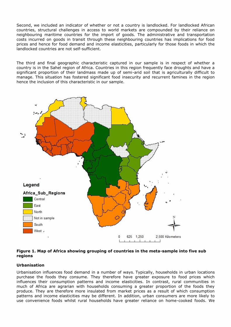
First, we identify five distinct geographic sub-regions of Africa namely North, Southern, East,
West and Central Africa. At the sub-regional level, strong commonalities in climate patterns
and soil characteristics across countries affects the suitability and yields of foods that are
grown in the regions. This may have implications for prices and taste, and thus demand for
locally grown foods as well as imported substitutes. Also cultural influences and proclivities for
foods are likely to be stronger across the countries making up a region.
Each country in our sample was assigned a region according to its membership of five main
sub-regional economic organisations namely the Arab Maghreb Union (UMA), Southern African
Development Community (SADC), East African Community (EAC), Economic Community of
West African States (ECOWAS) and the Economic Community of Central African States
(ECCAS). Some countries such as Egypt do not belong to any of these organisations but their
regional placement is unambiguous (i.e. North Africa). Other countries such as Angola,
Burundi, DR Congo and Tanzania4 belong to more than one of these organisations, perhaps
due to the ambiguity in their regional placements. For purposes of our analysis, we require
each country to be uniquely identified with a region. Thus these countries were assigned their
most appropriate region by considering the grouping used by the United Nations Statistical
Divisions (UNSD) of Africa. Angola and DR Congo were included within the Central region of
Africa, and Tanzania and Burundi in the Eastern region of Africa. Figure 1 shows our grouping
of countries in the meta-sampel into the five sub-regions.
4 Angola (SADC and ECCAS), Burundi (EAC and ECCAS), DR Congo (SADC and ECCAS) and Tanzania (SADC and EAC).
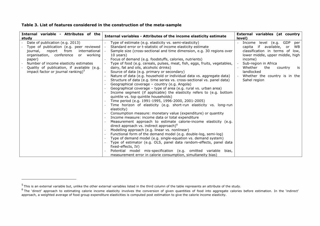
Table 3. List of features considered in the construction of the meta-sample
Internal variable - Attributes of the study
Internal variables - Attributes of the income elasticity estimate External variables (at country level)
- Date of publication (e.g. 2013) - Type of publication (e.g. peer reviewed
journal, report from international organisation, conference or working paper)
- Number of income elasticity estimates
- Quality of publication, if available (e.g.
impact factor or journal ranking)5
- Type of estimate (e.g. elasticity vs. semi-elasticity) - Standard error or t-statistic of income elasticity estimate - Sample size (cross-sectional and time dimension, e.g. 30 regions over
10 years) - Focus of demand (e.g. foodstuffs, calories, nutrients) - Type of food (e.g. cereals, pulses, meat, fish, eggs, fruits, vegetables,
dairy, fat and oils, alcoholic drinks)
- Source of data (e.g. primary or secondary) - Nature of data (e.g. household or individual data vs. aggregate data) - Structure of data (e.g. time series vs. cross-sectional vs. panel data) - Geographical coverage – country (e.g. Angola) - Geographical coverage – type of area (e.g. rural vs. urban area) - Income segment (if applicable) the elasticity refers to (e.g. bottom
quintile vs. top quintile households) - Time period (e.g. 1991-1995, 1996-2000, 2001-2005) - Time horizon of elasticity (e.g. short-run elasticity vs. long-run
elasticity) - Consumption measure: monetary value (expenditure) or quantity - Income measure: income data or total expenditure
- Measurement approach to estimate calorie-income elasticity (e.g.
direct approach vs. indirect approach)6 - Modelling approach (e.g. linear vs. nonlinear) - Functional form of the demand model (e.g. double-log, semi-log) - Type of demand model (e.g. single-equation vs. demand system) - Type of estimator (e.g. OLS, panel data random-effects, panel data
fixed-effects, IV)
- Potential model mis-specification (e.g. omitted variable bias, measurement error in calorie consumption, simultaneity bias)
- Income level (e.g. GDP per capita if available, or WB classification in terms of low, lower middle, upper middle, high income)
- Sub-region in Africa
- Whether the country is
landlocked - Whether the country is in the
Sahel region
5 This is an external variable but, unlike the other external variables listed in the third column of the table represents an attribute of the study. 6 The ‘direct’ approach to estimating calorie income elasticity involves the conversion of given quantities of food into aggregate calories before estimation. In the ‘indirect’
approach, a weighted average of food group expenditure elasticities is computed post estimation to give the calorie income elasticity.
Second, we included an indicator of whether or not a country is landlocked. For landlocked African
countries, structural challenges in access to world markets are compounded by their reliance on
neighbouring maritime countries for the import of goods. The administrative and transportation
costs incurred on goods in transit through these neighbouring countries has implications for food
prices and hence for food demand and income elasticities, particularly for those foods in which the
landlocked countries are not self-sufficient.
The third and final geographic characteristic captured in our sample is in respect of whether a
country is in the Sahel region of Africa. Countries in this region frequently face droughts and have a
significant proportion of their landmass made up of semi-arid soil that is agriculturally difficult to
manage. This situation has fostered significant food insecurity and recurrent famines in the region
hence the inclusion of this characteristic in our sample.
Figure 1. Map of Africa showing grouping of countries in the meta-sample into five sub
regions
Urbanisation
Urbanisation influences food demand in a number of ways. Typically, households in urban locations
purchase the foods they consume. They therefore have greater exposure to food prices which
influences their consumption patterns and income elasticities. In contrast, rural communities in
much of Africa are agrarian with households consuming a greater proportion of the foods they
produce. They are therefore more insulated from market prices as a result of which consumption
patterns and income elasticities may be different. In addition, urban consumers are more likely to
use convenience foods whilst rural households have greater reliance on home-cooked foods. We
include a measure of urbanisation based on the percentage of population in urban areas. This is high
in countries such as Nigeria and South Africa which have very large and densely populated mega
cities. Urbanisation data were taken from the World Development Indicators dataset (World Bank
WDI, 2015). For studies using panel and time series data, we take the average of these variables for
the period of the data in the underlying study.
National income
The level of a country’s income determines the amount as well as composition of its food demand.
On average, high income countries spend 16% of their incomes on food while low income countries
spend 55% (Regmi et al., 2001). Low income countries are therefore more responsive to volatility in
food prices and income shocks especially for the high value products. To control for the effects of
countries’ income levels on the variation of income elasticities across studies, we include each
country’s income level in our meta-sample according to the year of the data used in the underlying
studies. For completeness, two indicators of income from the World Bank’s WDI data are considered.
The first is the gross domestic product per capita (GDP pc) which is provided in constant 2005 dollar
terms7. For studies using panel and time series data, we take the average of these incomes for the
period of the data in the underlying study. The second is based on the World Bank’s income
classification of countries into low (L), lower middle (LM), upper middle (UM) and high (H) income
levels. For time series and panel data, we use the most frequent occurring classification in the
underlying study’s data period. Our preference is to use the GDP pc indicator, but we were conscious
that a lack of sufficient data may require the use of the proxy based on income classification.
Journal Impact Factor
There is a potential inclination for peer reviewed journals to publish studies that find compelling
empirical results of a particular magnitude and/or statistical significance. If this inclination exists, it
engenders a situation where authors are tempted to submit their manuscripts according to an
established trend of published results. Papers based on poor data, or with inconclusive or weak
findings may not be submitted to high impact journals or may miss out in the competition for space
in those journals (Murtaugh, 2002). This preferential publication phenomenon may foster a
relationship between journal quality and the trend of published results. In meta-regression analysis,
it introduces so-called ‘publication bias’ which we aim to investigate.
To ascertain the relative quality of the journals in our sample, we first determined the 5-year
average impact factors of those that are present in the most recent Web of Science Journal Citation
Report (WoS JCR, 2014). These range from 0.50 (China Agricultural Economic Review) to 3.11
(Journal of Development Economics). However, 17 out of the 29 journals in our sample are not
present in the WoS JCR. Given the extensive coverage of the WoS JCR, it is reasonable to assume
that un-represented journals are generally of lower quality. To standardise our ranking therefore, we
created an internal ordinal scale and classify all the journals that are not represented in the WoS
JCR in the lower end of that scale. As shown in Table 4 below, these are ranked 1 (i.e. lowest).
Following this, four bands were then created and an internal ranking of journals was established
according to the appropriate range of their impact factors.
7 We could not use GDP pc in PPP terms due to insufficient data.
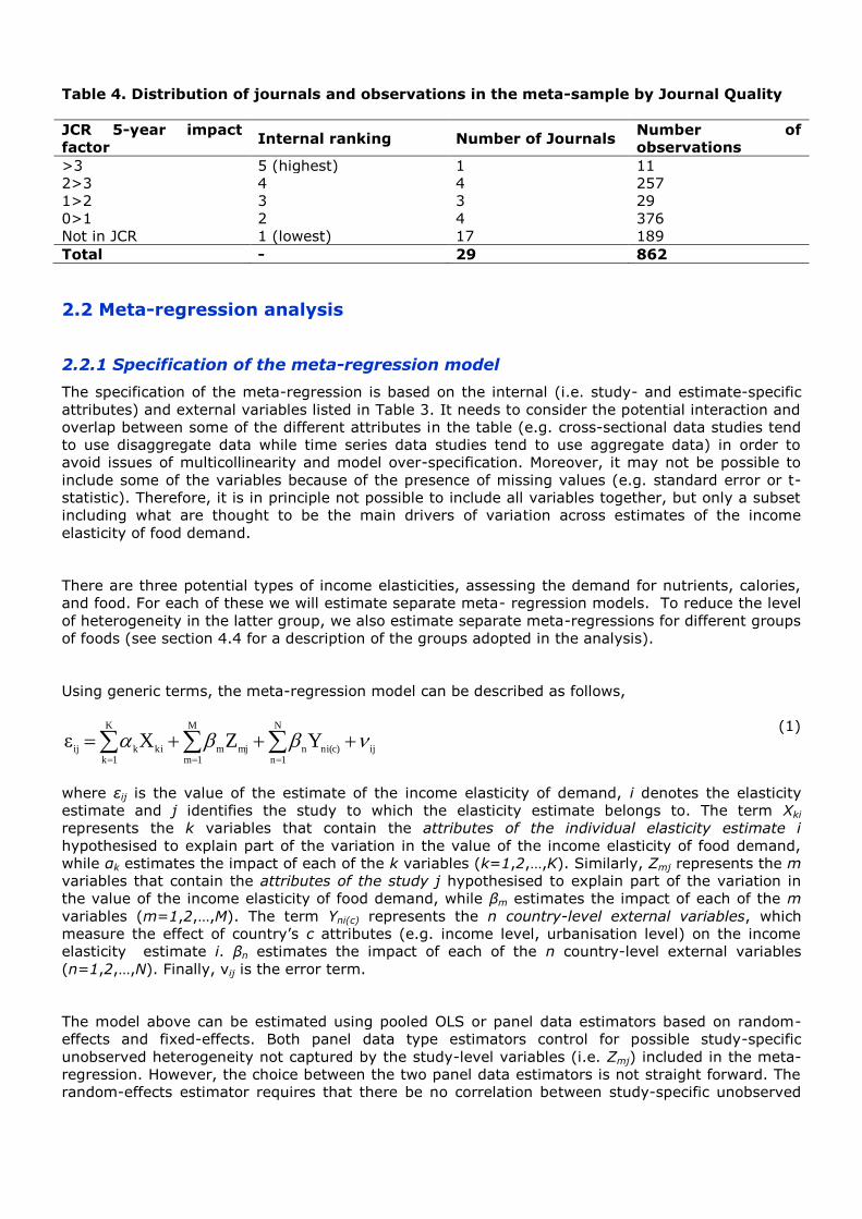
Table 4. Distribution of journals and observations in the meta-sample by Journal Quality
JCR 5-year impact
factor Internal ranking Number of Journals
Number of
observations
>3 5 (highest) 1 11
2>3 4 4 257
1>2 3 3 29
0>1 2 4 376
Not in JCR 1 (lowest) 17 189
Total - 29 862
2.2 Meta-regression analysis
2.2.1 Specification of the meta-regression model
The specification of the meta-regression is based on the internal (i.e. study- and estimate-specific
attributes) and external variables listed in Table 3. It needs to consider the potential interaction and
overlap between some of the different attributes in the table (e.g. cross-sectional data studies tend
to use disaggregate data while time series data studies tend to use aggregate data) in order to
avoid issues of multicollinearity and model over-specification. Moreover, it may not be possible to
include some of the variables because of the presence of missing values (e.g. standard error or t-
statistic). Therefore, it is in principle not possible to include all variables together, but only a subset
including what are thought to be the main drivers of variation across estimates of the income
elasticity of food demand.
There are three potential types of income elasticities, assessing the demand for nutrients, calories,
and food. For each of these we will estimate separate meta- regression models. To reduce the level
of heterogeneity in the latter group, we also estimate separate meta-regressions for different groups
of foods (see section 4.4 for a description of the groups adopted in the analysis).
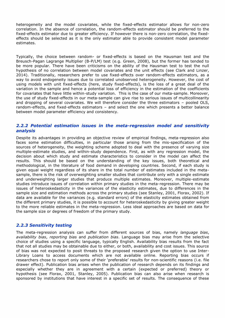
Using generic terms, the meta-regression model can be described as follows,
ij
N
1nni(c)n
M
1mmjm
K
1kkikij
YZXε
(1)
where εij is the value of the estimate of the income elasticity of demand, i denotes the elasticity
estimate and j identifies the study to which the elasticity estimate belongs to. The term Xki
represents the k variables that contain the attributes of the individual elasticity estimate i
hypothesised to explain part of the variation in the value of the income elasticity of food demand,
while αk estimates the impact of each of the k variables (k=1,2,…,K). Similarly, Zmj represents the m
variables that contain the attributes of the study j hypothesised to explain part of the variation in
the value of the income elasticity of food demand, while βm estimates the impact of each of the m
variables (m=1,2,…,M). The term Yni(c) represents the n country-level external variables, which
measure the effect of country’s c attributes (e.g. income level, urbanisation level) on the income
elasticity estimate i. βn estimates the impact of each of the n country-level external variables
(n=1,2,…,N). Finally, νij is the error term.
The model above can be estimated using pooled OLS or panel data estimators based on random-
effects and fixed-effects. Both panel data type estimators control for possible study-specific
unobserved heterogeneity not captured by the study-level variables (i.e. Zmj) included in the meta-
regression. However, the choice between the two panel data estimators is not straight forward. The
random-effects estimator requires that there be no correlation between study-specific unobserved
heterogeneity and the model covariates, while the fixed-effects estimator allows for non-zero
correlation. In the absence of correlation, the random-effects estimator should be preferred to the
fixed-effects estimator due to greater efficiency. If however there is non-zero correlation, the fixed-
effects should be selected as it is the only estimator able to provide consistent model parameter
estimates.
Typically, the choice between random- or fixed-effects is based on the Hausman test and the
Breusch-Pagan Lagrange Multiplier (B-P/LM) test (e.g. Green, 2008), but the former has tended to
be more popular. There have been criticisms on the ability of the Hausman test to test the null
hypothesis of no correlation between model covariates and the unit effects (see Clark and Linzer,
2014). Traditionally, researchers prefer to use fixed-effects over random-effects estimators, as a
way to avoid endogeneity issues due to correlated unobserved heterogeneity. However, the cost of
using models with unit fixed-effects (here, study fixed-effects), is the loss of a great deal of the
variation in the sample and hence a potential loss of efficiency in the estimation of the coefficients
for covariates that have little within-study variation. This is the case of our meta-sample. Moreover,
the use of study fixed-effects in our meta-sample can give rise to serious issues of multicollinearity
and dropping of several covariates. We will therefore consider the three estimators – pooled OLS,
random-effects, and fixed-effects estimators – and select the one which presents a better balance
between model parameter efficiency and consistency.
2.2.2 Potential estimation issues in the meta-regression model and sensitivity
analysis
Despite its advantages in providing an objective review of empirical findings, meta-regression also
faces some estimation difficulties, in particular those arising from the mis-specification of the
sources of heterogeneity, the weighting scheme adopted to deal with the presence of varying size
multiple-estimate studies, and within-study dependence. First, as with any regression model, the
decision about which study and estimate characteristics to consider in the model can affect the
results. This should be based on the understanding of the key issues, both theoretical and
methodological, in the literature of food demand in developing countries. Second, if each study is
given equal weight regardless of its share in the total number of estimates included in the meta-
sample, there is the risk of overweighting smaller studies that contribute only with a single estimate
and underweighting larger studies that produce multiple estimates. Moreover, multiple-estimate
studies introduce issues of correlation within primary studies in the meta-regression. There may be
issues of heteroskedasticity in the variances of the elasticity estimates, due to differences in the
sample size and estimation methods across the primary studies (see Stanley, 2001, Florax, 2002). If
data are available for the variances (e.g. standard errors) of the elasticity estimates obtained from
the different primary studies, it is possible to account for heteroskedasticity by giving greater weight
to the more reliable estimates in the meta-regression. Less ideal approaches are based on data for
the sample size or degrees of freedom of the primary study.
2.2.3 Sensitivity testing
The meta-regression analysis can suffer from different sources of bias, namely language bias,
availability bias, reporting bias and publication bias. Language bias may arise from the selective
choice of studies using a specific language, typically English. Availability bias results from the fact
that not all studies may be obtainable due to either, or both, availability and cost issues. This source
of bias was not expected to posit threats to the proposed research given the option to use Inter-
Library Loans to access documents which are not available online. Reporting bias occurs if
researchers chose to report only some of their ‘preferable’ results for non-scientific reasons (i.e. file
drawer effect). Publication bias arises when the publication of research depends on its findings and
especially whether they are in agreement with a certain (expected or preferred) theory or
hypothesis (see Florax, 2001, Stanley, 2005). Publication bias can also arise when research is
sponsored by institutions that have interest in a specific set of results. The consequence of these
different sources of bias is that the empirical literature included in the meta-regression may not be
representative of the whole population of studies undertaken on a given topic.
Perhaps the most concerning issue is that of publication bias. One simple sensitivity test can be to
consider the impact of including separate categories for type of publication (e.g. peer reviewed
studies vs. ‘grey’ literature) and type of research sponsor (e.g. academic institution vs. international
organisation). The presence of significant differences between groups may be indicative of
publication bias. It is also possible to test whether there appears to be a systematic relationship
between journal impact factor (or an indicator of journal ranking) and the income elasticity
estimates, for the sample containing estimates from peer reviewed journals. In addition, visual
inspection of the association between the (absolute) value of the income elasticity estimates and
their respective standard errors for peer reviewed studies and ‘grey’ literature, separately, may also
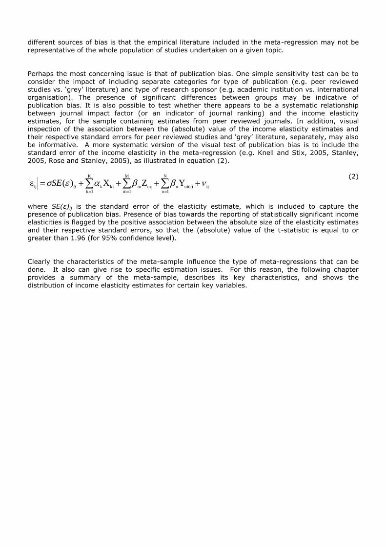
be informative. A more systematic version of the visual test of publication bias is to include the
standard error of the income elasticity in the meta-regression (e.g. Knell and Stix, 2005, Stanley,
2005, Rose and Stanley, 2005), as illustrated in equation (2).
ij
N
1nni(c)n
M
1mmjm
K
1kkikij
YZX)(ε
ijSE
(2)
where SE(ε)ij is the standard error of the elasticity estimate, which is included to capture the
presence of publication bias. Presence of bias towards the reporting of statistically significant income
elasticities is flagged by the positive association between the absolute size of the elasticity estimates
and their respective standard errors, so that the (absolute) value of the t-statistic is equal to or
greater than 1.96 (for 95% confidence level).
Clearly the characteristics of the meta-sample influence the type of meta-regressions that can be
done. It also can give rise to specific estimation issues. For this reason, the following chapter
provides a summary of the meta-sample, describes its key characteristics, and shows the
distribution of income elasticity estimates for certain key variables.
3. Description of the meta-sample
3.1 Studies included in the meta-sample
This chapter provides an overview of the meta-sample with full information provided in the
spreadsheet. There were 89 candidate studies selected to be included in the meta-sample. Of these,
23 studies were excluded for different reasons, namely: inappropriate dependent variable (3
studies), inaccessible articles (9 studies)8, unrelated subject matter (4 studies), elasticity estimates
not reported in the study (6 studies), and non-African country (1 study). As a consequence, 66
(about 74% of all studies) have been fully included in the meta-sample reporting a total of 2,101
elasticity estimates.
Of the 66 studies included, 43 are studies which have not been included in previous meta-analyses.
11 studies were produced by international organizations (9 of which are from IFPRI), 10 are working
papers, while the remaining 45 are studies published in peer reviewed journals. Note that all studies
considered in the final sample are in English, despite having specified search terms in Portugues,
French and Spanish as well. Altogether, 48 out of 54 African countries are represented in our
sample although some have few observations. Appendix A lists the studies included in the meta-
sample, Appendix B those selected but subsequently excluded from the analysis.
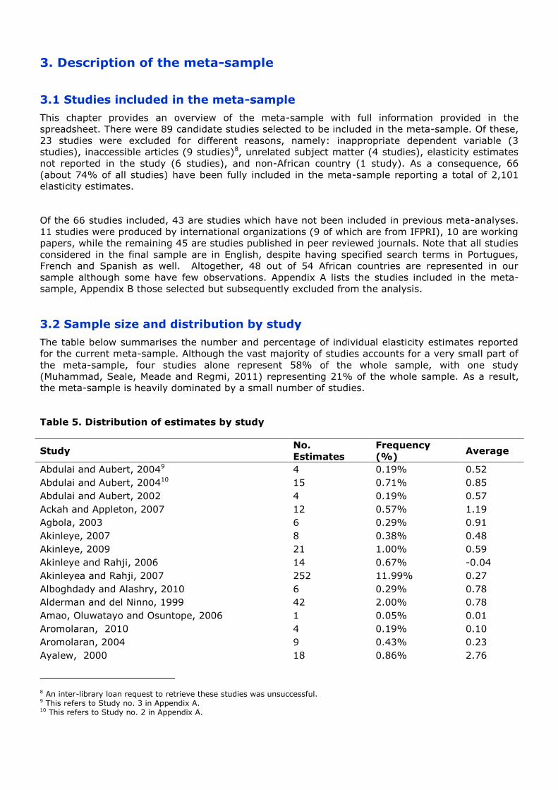
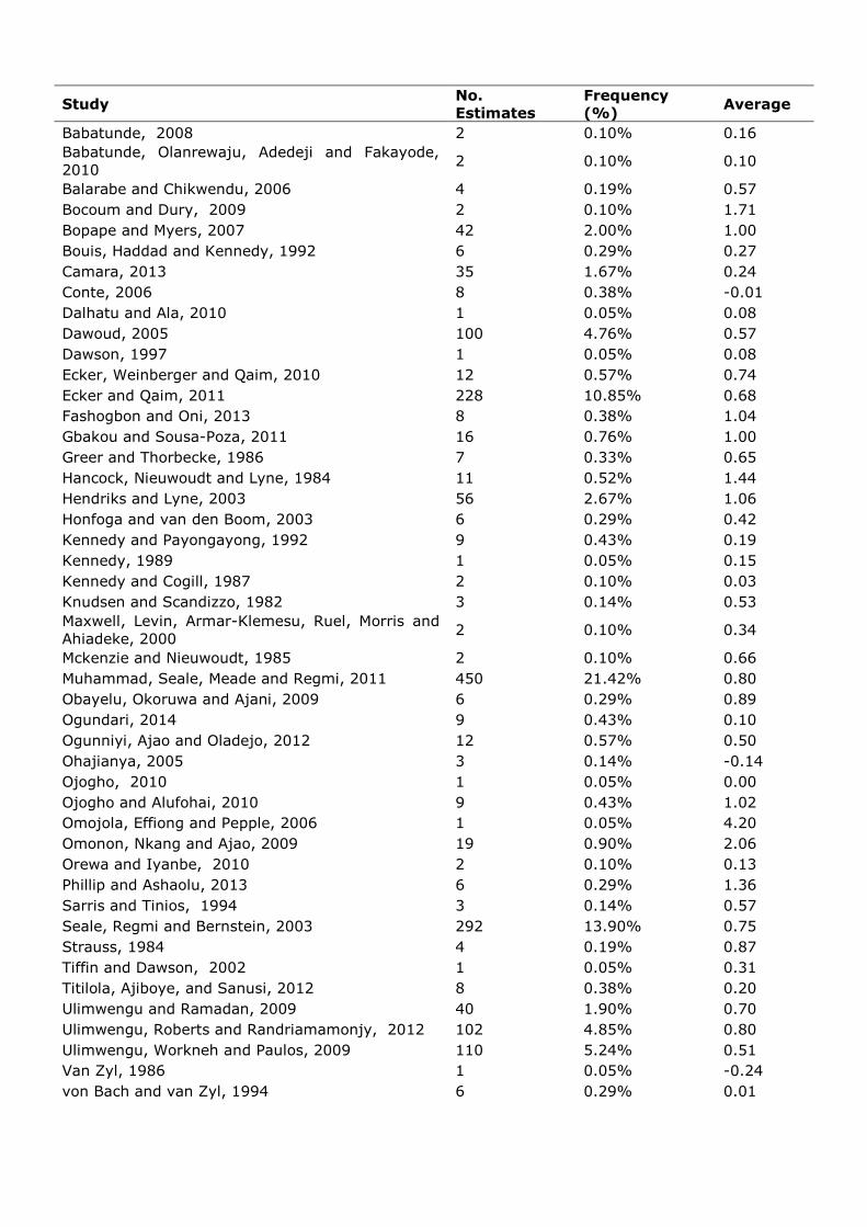
3.2 Sample size and distribution by study
The table below summarises the number and percentage of individual elasticity estimates reported
for the current meta-sample. Although the vast majority of studies accounts for a very small part of
the meta-sample, four studies alone represent 58% of the whole sample, with one study
(Muhammad, Seale, Meade and Regmi, 2011) representing 21% of the whole sample. As a result,
the meta-sample is heavily dominated by a small number of studies.
Table 5. Distribution of estimates by study
Study No.
Estimates
Frequency
(%) Average
Abdulai and Aubert, 20049 4 0.19% 0.52
Abdulai and Aubert, 200410 15 0.71% 0.85
Abdulai and Aubert, 2002 4 0.19% 0.57
Ackah and Appleton, 2007 12 0.57% 1.19
Agbola, 2003 6 0.29% 0.91
Akinleye, 2007 8 0.38% 0.48
Akinleye, 2009 21 1.00% 0.59
Akinleye and Rahji, 2006 14 0.67% -0.04
Akinleyea and Rahji, 2007 252 11.99% 0.27
Alboghdady and Alashry, 2010 6 0.29% 0.78
Alderman and del Ninno, 1999 42 2.00% 0.78
Amao, Oluwatayo and Osuntope, 2006 1 0.05% 0.01
Aromolaran, 2010 4 0.19% 0.10
Aromolaran, 2004 9 0.43% 0.23
Ayalew, 2000 18 0.86% 2.76
8 An inter-library loan request to retrieve these studies was unsuccessful. 9 This refers to Study no. 3 in Appendix A. 10 This refers to Study no. 2 in Appendix A.
Study No.
Estimates
Frequency
(%) Average
Babatunde, 2008 2 0.10% 0.16
Babatunde, Olanrewaju, Adedeji and Fakayode,
2010 2 0.10% 0.10
Balarabe and Chikwendu, 2006 4 0.19% 0.57
Bocoum and Dury, 2009 2 0.10% 1.71
Bopape and Myers, 2007 42 2.00% 1.00
Bouis, Haddad and Kennedy, 1992 6 0.29% 0.27
Camara, 2013 35 1.67% 0.24
Conte, 2006 8 0.38% -0.01
Dalhatu and Ala, 2010 1 0.05% 0.08
Dawoud, 2005 100 4.76% 0.57
Dawson, 1997 1 0.05% 0.08
Ecker, Weinberger and Qaim, 2010 12 0.57% 0.74
Ecker and Qaim, 2011 228 10.85% 0.68
Fashogbon and Oni, 2013 8 0.38% 1.04
Gbakou and Sousa-Poza, 2011 16 0.76% 1.00
Greer and Thorbecke, 1986 7 0.33% 0.65
Hancock, Nieuwoudt and Lyne, 1984 11 0.52% 1.44
Hendriks and Lyne, 2003 56 2.67% 1.06
Honfoga and van den Boom, 2003 6 0.29% 0.42
Kennedy and Payongayong, 1992 9 0.43% 0.19
Kennedy, 1989 1 0.05% 0.15
Kennedy and Cogill, 1987 2 0.10% 0.03
Knudsen and Scandizzo, 1982 3 0.14% 0.53
Maxwell, Levin, Armar-Klemesu, Ruel, Morris and
Ahiadeke, 2000 2 0.10% 0.34
Mckenzie and Nieuwoudt, 1985 2 0.10% 0.66
Muhammad, Seale, Meade and Regmi, 2011 450 21.42% 0.80
Obayelu, Okoruwa and Ajani, 2009 6 0.29% 0.89
Ogundari, 2014 9 0.43% 0.10
Ogunniyi, Ajao and Oladejo, 2012 12 0.57% 0.50
Ohajianya, 2005 3 0.14% -0.14
Ojogho, 2010 1 0.05% 0.00
Ojogho and Alufohai, 2010 9 0.43% 1.02
Omojola, Effiong and Pepple, 2006 1 0.05% 4.20
Omonon, Nkang and Ajao, 2009 19 0.90% 2.06
Orewa and Iyanbe, 2010 2 0.10% 0.13
Phillip and Ashaolu, 2013 6 0.29% 1.36
Sarris and Tinios, 1994 3 0.14% 0.57
Seale, Regmi and Bernstein, 2003 292 13.90% 0.75
Strauss, 1984 4 0.19% 0.87
Tiffin and Dawson, 2002 1 0.05% 0.31
Titilola, Ajiboye, and Sanusi, 2012 8 0.38% 0.20
Ulimwengu and Ramadan, 2009 40 1.90% 0.70
Ulimwengu, Roberts and Randriamamonjy, 2012 102 4.85% 0.80
Ulimwengu, Workneh and Paulos, 2009 110 5.24% 0.51
Van Zyl, 1986 1 0.05% -0.24
von Bach and van Zyl, 1994 6 0.29% 0.01
Study No.
Estimates
Frequency
(%) Average
von Braun, de Haen and Blanke, 1991 16 0.76% 1.69
von Braun, Puetz and Webb, 1989 2 0.10% 0.43
Weliwita, Nyange and Tsujii, 2003 12 0.57% 0.99
Yusuf, 2012 3 0.14% 0.93
Grand Total 2,101 100.00% 0.70
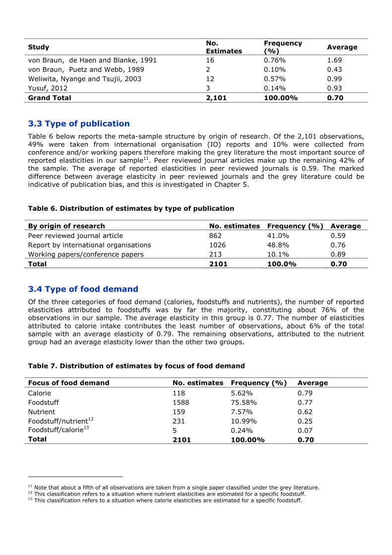
3.3 Type of publication
Table 6 below reports the meta-sample structure by origin of research. Of the 2,101 observations,
49% were taken from international organisation (IO) reports and 10% were collected from
conference and/or working papers therefore making the grey literature the most important source of
reported elasticities in our sample11. Peer reviewed journal articles make up the remaining 42% of
the sample. The average of reported elasticities in peer reviewed journals is 0.59. The marked
difference between average elasticity in peer reviewed journals and the grey literature could be
indicative of publication bias, and this is investigated in Chapter 5.
Table 6. Distribution of estimates by type of publication
By origin of research No. estimates Frequency (%) Average
Peer reviewed journal article 862 41.0% 0.59
Report by international organisations 1026 48.8% 0.76
Working papers/conference papers 213 10.1% 0.89
Total 2101 100.0% 0.70
3.4 Type of food demand
Of the three categories of food demand (calories, foodstuffs and nutrients), the number of reported
elasticities attributed to foodstuffs was by far the majority, constituting about 76% of the
observations in our sample. The average elasticity in this group is 0.77. The number of elasticities
attributed to calorie intake contributes the least number of observations, about 6% of the total
sample with an average elasticity of 0.79. The remaining observations, attributed to the nutrient
group had an average elasticity lower than the other two groups.
Table 7. Distribution of estimates by focus of food demand
Focus of food demand No. estimates Frequency (%) Average
Calorie 118 5.62% 0.79
Foodstuff 1588 75.58% 0.77
Nutrient 159 7.57% 0.62
Foodstuff/nutrient12 231 10.99% 0.25
Foodstuff/calorie13 5 0.24% 0.07
Total 2101 100.00% 0.70
11 Note that about a fifth of all observations are taken from a single paper classified under the grey literature. 12 This classification refers to a situation where nutrient elasticities are estimated for a specific foodstuff. 13 This classification refers to a situation where calorie elasticities are estimated for a specific foodstuff.
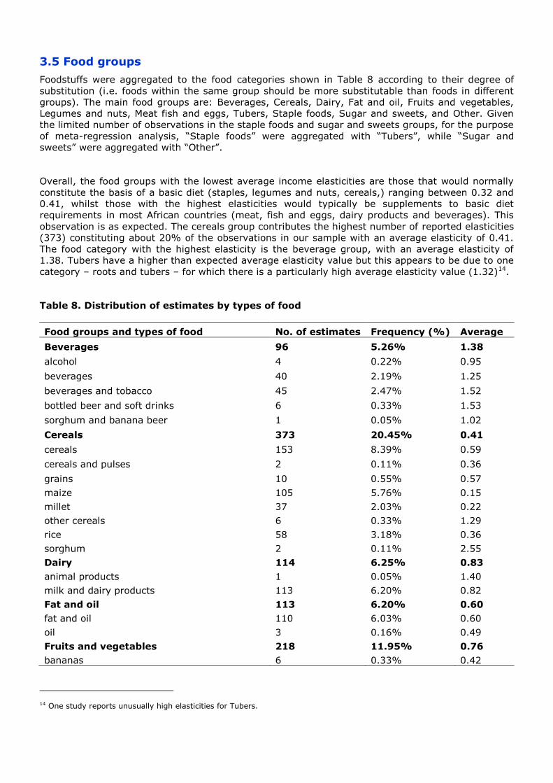
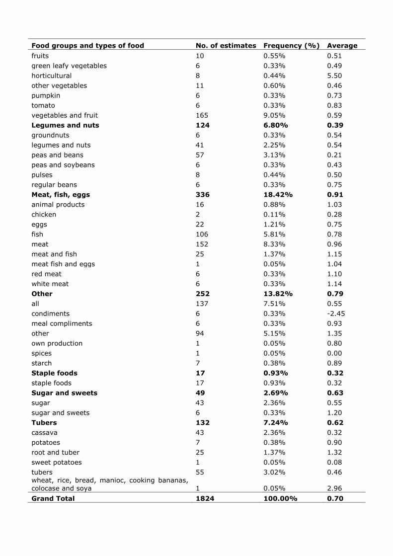
3.5 Food groups
Foodstuffs were aggregated to the food categories shown in Table 8 according to their degree of
substitution (i.e. foods within the same group should be more substitutable than foods in different
groups). The main food groups are: Beverages, Cereals, Dairy, Fat and oil, Fruits and vegetables,
Legumes and nuts, Meat fish and eggs, Tubers, Staple foods, Sugar and sweets, and Other. Given
the limited number of observations in the staple foods and sugar and sweets groups, for the purpose
of meta-regression analysis, “Staple foods” were aggregated with “Tubers”, while “Sugar and
sweets” were aggregated with “Other”.
Overall, the food groups with the lowest average income elasticities are those that would normally
constitute the basis of a basic diet (staples, legumes and nuts, cereals,) ranging between 0.32 and
0.41, whilst those with the highest elasticities would typically be supplements to basic diet
requirements in most African countries (meat, fish and eggs, dairy products and beverages). This
observation is as expected. The cereals group contributes the highest number of reported elasticities
(373) constituting about 20% of the observations in our sample with an average elasticity of 0.41.
The food category with the highest elasticity is the beverage group, with an average elasticity of
1.38. Tubers have a higher than expected average elasticity value but this appears to be due to one
category – roots and tubers – for which there is a particularly high average elasticity value (1.32)14.
Table 8. Distribution of estimates by types of food
Food groups and types of food No. of estimates Frequency (%) Average
Beverages 96 5.26% 1.38
alcohol 4 0.22% 0.95
beverages 40 2.19% 1.25
beverages and tobacco 45 2.47% 1.52
bottled beer and soft drinks 6 0.33% 1.53
sorghum and banana beer 1 0.05% 1.02
Cereals 373 20.45% 0.41
cereals 153 8.39% 0.59
cereals and pulses 2 0.11% 0.36
grains 10 0.55% 0.57
maize 105 5.76% 0.15
millet 37 2.03% 0.22
other cereals 6 0.33% 1.29
rice 58 3.18% 0.36
sorghum 2 0.11% 2.55
Dairy 114 6.25% 0.83
animal products 1 0.05% 1.40
milk and dairy products 113 6.20% 0.82
Fat and oil 113 6.20% 0.60
fat and oil 110 6.03% 0.60
oil 3 0.16% 0.49
Fruits and vegetables 218 11.95% 0.76
bananas 6 0.33% 0.42
14 One study reports unusually high elasticities for Tubers.
Food groups and types of food No. of estimates Frequency (%) Average
fruits 10 0.55% 0.51
green leafy vegetables 6 0.33% 0.49
horticultural 8 0.44% 5.50
other vegetables 11 0.60% 0.46
pumpkin 6 0.33% 0.73
tomato 6 0.33% 0.83
vegetables and fruit 165 9.05% 0.59
Legumes and nuts 124 6.80% 0.39
groundnuts 6 0.33% 0.54
legumes and nuts 41 2.25% 0.54
peas and beans 57 3.13% 0.21
peas and soybeans 6 0.33% 0.43
pulses 8 0.44% 0.50
regular beans 6 0.33% 0.75
Meat, fish, eggs 336 18.42% 0.91
animal products 16 0.88% 1.03
chicken 2 0.11% 0.28
eggs 22 1.21% 0.75
fish 106 5.81% 0.78
meat 152 8.33% 0.96
meat and fish 25 1.37% 1.15
meat fish and eggs 1 0.05% 1.04
red meat 6 0.33% 1.10
white meat 6 0.33% 1.14
Other 252 13.82% 0.79
all 137 7.51% 0.55
condiments 6 0.33% -2.45
meal compliments 6 0.33% 0.93
other 94 5.15% 1.35
own production 1 0.05% 0.80
spices 1 0.05% 0.00
starch 7 0.38% 0.89
Staple foods 17 0.93% 0.32
staple foods 17 0.93% 0.32
Sugar and sweets 49 2.69% 0.63
sugar 43 2.36% 0.55
sugar and sweets 6 0.33% 1.20
Tubers 132 7.24% 0.62
cassava 43 2.36% 0.32
potatoes 7 0.38% 0.90
root and tuber 25 1.37% 1.32
sweet potatoes 1 0.05% 0.08
tubers 55 3.02% 0.46
wheat, rice, bread, manioc, cooking bananas,
colocase and soya 1 0.05% 2.96
Grand Total 1824 100.00% 0.70
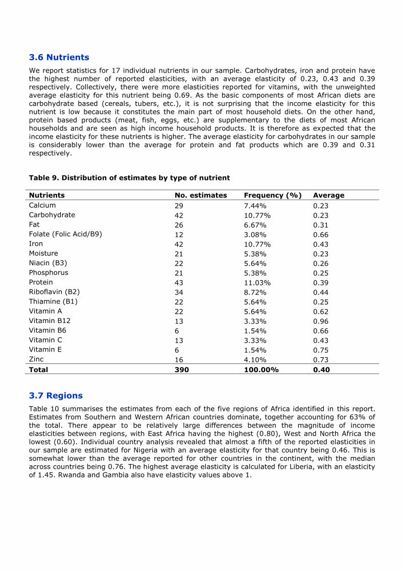
3.6 Nutrients
We report statistics for 17 individual nutrients in our sample. Carbohydrates, iron and protein have
the highest number of reported elasticities, with an average elasticity of 0.23, 0.43 and 0.39
respectively. Collectively, there were more elasticities reported for vitamins, with the unweighted
average elasticity for this nutrient being 0.69. As the basic components of most African diets are
carbohydrate based (cereals, tubers, etc.), it is not surprising that the income elasticity for this
nutrient is low because it constitutes the main part of most household diets. On the other hand,
protein based products (meat, fish, eggs, etc.) are supplementary to the diets of most African
households and are seen as high income household products. It is therefore as expected that the
income elasticity for these nutrients is higher. The average elasticity for carbohydrates in our sample
is considerably lower than the average for protein and fat products which are 0.39 and 0.31
respectively.
Table 9. Distribution of estimates by type of nutrient
Nutrients No. estimates Frequency (%) Average
Calcium 29 7.44% 0.23
Carbohydrate 42 10.77% 0.23
Fat 26 6.67% 0.31
Folate (Folic Acid/B9) 12 3.08% 0.66
Iron 42 10.77% 0.43
Moisture 21 5.38% 0.23
Niacin (B3) 22 5.64% 0.26
Phosphorus 21 5.38% 0.25
Protein 43 11.03% 0.39
Riboflavin (B2) 34 8.72% 0.44
Thiamine (B1) 22 5.64% 0.25
Vitamin A 22 5.64% 0.62
Vitamin B12 13 3.33% 0.96
Vitamin B6 6 1.54% 0.66
Vitamin C 13 3.33% 0.43
Vitamin E 6 1.54% 0.75
Zinc 16 4.10% 0.73
Total 390 100.00% 0.40
3.7 Regions
Table 10 summarises the estimates from each of the five regions of Africa identified in this report.
Estimates from Southern and Western African countries dominate, together accounting for 63% of
the total. There appear to be relatively large differences between the magnitude of income
elasticities between regions, with East Africa having the highest (0.80), West and North Africa the
lowest (0.60). Individual country analysis revealed that almost a fifth of the reported elasticities in
our sample are estimated for Nigeria with an average elasticity for that country being 0.46. This is
somewhat lower than the average reported for other countries in the continent, with the median
across countries being 0.76. The highest average elasticity is calculated for Liberia, with an elasticity
of 1.45. Rwanda and Gambia also have elasticity values above 1.
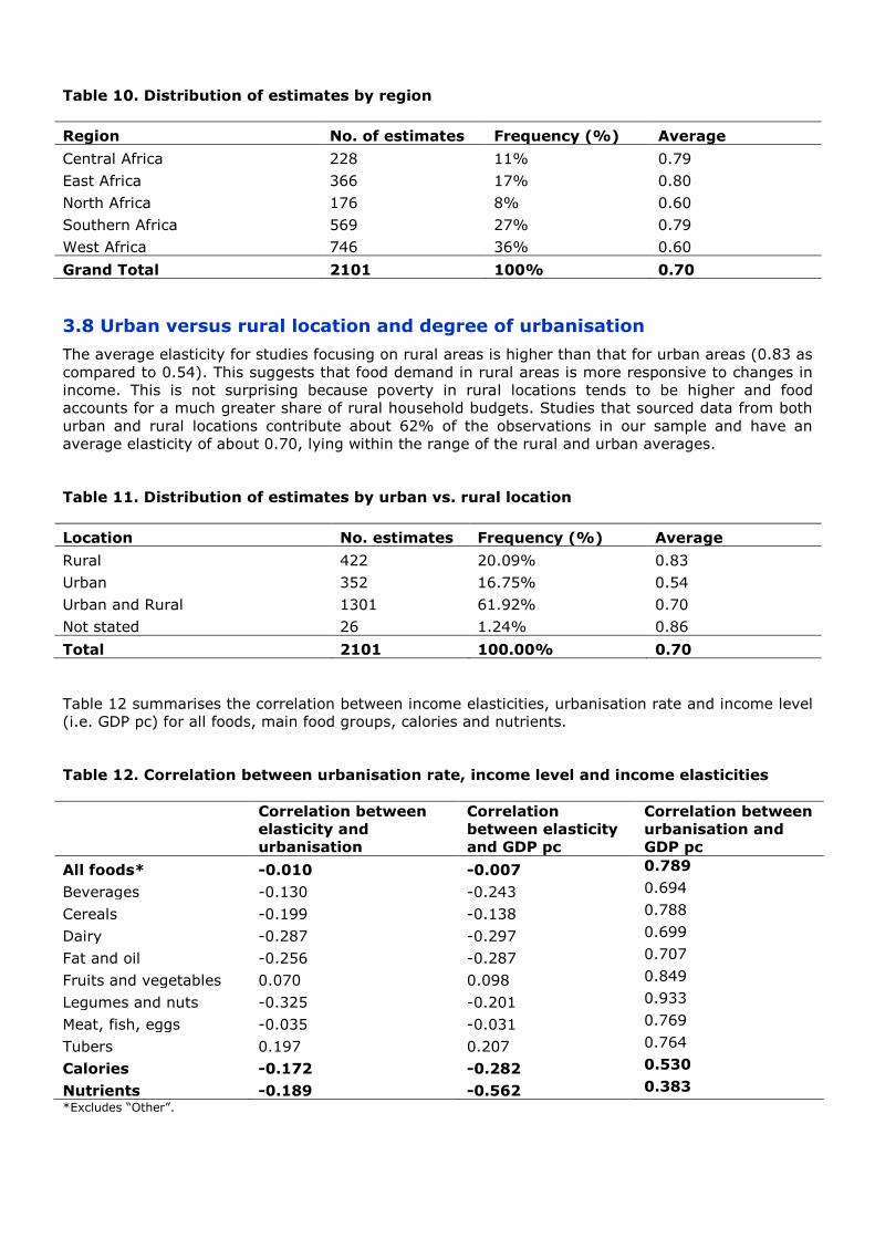
Table 10. Distribution of estimates by region
Region No. of estimates Frequency (%) Average
Central Africa 228 11% 0.79
East Africa 366 17% 0.80
North Africa 176 8% 0.60
Southern Africa 569 27% 0.79
West Africa 746 36% 0.60
Grand Total 2101 100% 0.70
3.8 Urban versus rural location and degree of urbanisation
The average elasticity for studies focusing on rural areas is higher than that for urban areas (0.83 as
compared to 0.54). This suggests that food demand in rural areas is more responsive to changes in
income. This is not surprising because poverty in rural locations tends to be higher and food
accounts for a much greater share of rural household budgets. Studies that sourced data from both
urban and rural locations contribute about 62% of the observations in our sample and have an
average elasticity of about 0.70, lying within the range of the rural and urban averages.
Table 11. Distribution of estimates by urban vs. rural location
Location No. estimates Frequency (%) Average
Rural 422 20.09% 0.83
Urban 352 16.75% 0.54
Urban and Rural 1301 61.92% 0.70
Not stated 26 1.24% 0.86
Total 2101 100.00% 0.70
Table 12 summarises the correlation between income elasticities, urbanisation rate and income level
(i.e. GDP pc) for all foods, main food groups, calories and nutrients.
Table 12. Correlation between urbanisation rate, income level and income elasticities
Correlation between
elasticity and
urbanisation
Correlation
between elasticity
and GDP pc
Correlation between
urbanisation and
GDP pc
All foods* -0.010 -0.007 0.789
Beverages -0.130 -0.243 0.694
Cereals -0.199 -0.138 0.788
Dairy -0.287 -0.297 0.699
Fat and oil -0.256 -0.287 0.707
Fruits and vegetables 0.070 0.098 0.849
Legumes and nuts -0.325 -0.201 0.933
Meat, fish, eggs -0.035 -0.031 0.769
Tubers 0.197 0.207 0.764
Calories -0.172 -0.282 0.530
Nutrients -0.189 -0.562 0.383
*Excludes “Other”.
Overall, the coefficients indicate that increased urbanisation (measured as the share of the country’s
population living in urben areas) is associated with lower income elasticities (with only few
exceptions); increased levels of income (in terms of GDP per capita) also tend to be associated with
lower income elasticities (with only few exceptions), and that there is a positive association between
country’s urbanisation rate and income level.
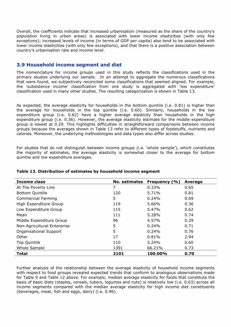
3.9 Household income segment and diet
The nomenclature for income groups used in this study reflects the classifications used in the
primary studies underlying our sample. In an attempt to aggregate the numerous classifications
that were found, we subjectively reconciled some classifications that seemed aligned. For example,
the ‘subsistence income’ classification from one study is aggregated with ‘low expenditure’
classification used in many other studies. The resulting categorization is shown in Table 13.
As expected, the average elasticity for households in the bottom quintile (i.e. 0.81) is higher than
the average for households in the top quintile (i.e. 0.60). Similarly, households in the low
expenditure group (i.e. 0.62) have a higher average elasticity than households in the high
expenditure group (i.e. 0.36). However, the average elasticity estimate for the middle expenditure
group is lowest at 0.29. This highlights difficulties in straightforward comparisons between income
groups because the averages shown in Table 13 refer to different types of foodstuffs, nutrients and
calories. Moreover, the underlying methodologies and data types also differ across studies.
For studies that do not distinguish between income groups (i.e. ‘whole sample’), which constitutes
the majority of estimates, the average elasticity is somewhat closer to the average for bottom
quintile and low expenditure averages.
Table 13. Distribution of estimates by household income segment
Income class No. estimates Frequency (%) Average
At The Poverty Line 7 0.33% 0.65
Bottom Quintile 120 5.71% 0.81
Commercial Farming 5 0.24% 0.69
High Expenditure Group 119 5.66% 0.36
Low Expenditure Group 115 5.47% 0.62
Mean 111 5.28% 0.74
Middle Expenditure Group 96 4.57% 0.29
Non-Agricultural Enterprise 5 0.24% 0.71
Organisational Support 5 0.24% 0.76
Other 17 0.81% 2.94
Top Quintile 110 5.24% 0.60
Whole Sample 1391 66.21% 0.73
Total 2101 100.00% 0.70
Further analysis of the relationship between the average elasticity of household income segments
with respect to food groups revealed expected trends that conform to analogous observations made
for Table 9 and Table 12 above. For example, median average elasticity for foods that constitute the
basis of basic diets (staples, cereals, tubers, legumes and nuts) is relatively low (i.e. 0.63) across all
income segments compared with the median average elasticity for high income diet constituents
(beverages, meat, fish and eggs, dairy) (i.e. 0.96).
With regards differentiation in the income elasticity of foods that constitute basic diets, poorer
households have higher median responses (i.e. 0.55) than wealthier households (i.e. 0.39).
Similarly, for higher end food products, median elasticity of poorer households is higher (i.e. 1.13)
than for wealthier households (i.e.0.92). Again this trend conforms to the observations made
previously and is consistent with broader observations of dietary convergence as income levels rise.
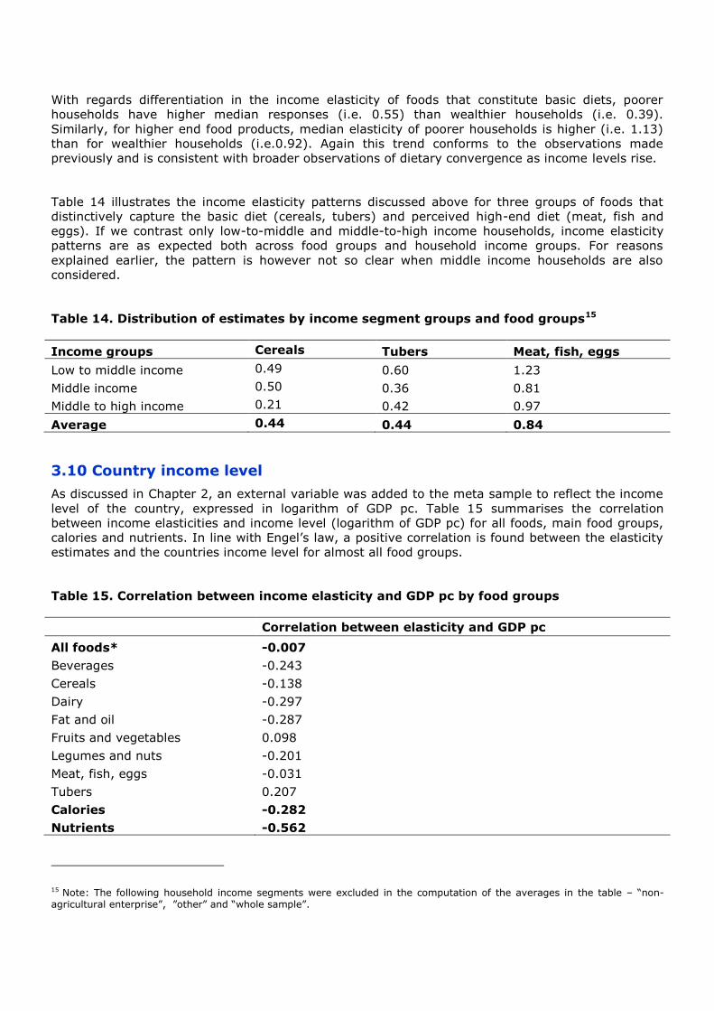
Table 14 illustrates the income elasticity patterns discussed above for three groups of foods that
distinctively capture the basic diet (cereals, tubers) and perceived high-end diet (meat, fish and
eggs). If we contrast only low-to-middle and middle-to-high income households, income elasticity
patterns are as expected both across food groups and household income groups. For reasons
explained earlier, the pattern is however not so clear when middle income households are also
considered.
Table 14. Distribution of estimates by income segment groups and food groups15
Income groups Cereals Tubers Meat, fish, eggs
Low to middle income 0.49 0.60 1.23
Middle income 0.50 0.36 0.81
Middle to high income 0.21 0.42 0.97
Average 0.44 0.44 0.84
3.10 Country income level
As discussed in Chapter 2, an external variable was added to the meta sample to reflect the income
level of the country, expressed in logarithm of GDP pc. Table 15 summarises the correlation
between income elasticities and income level (logarithm of GDP pc) for all foods, main food groups,
calories and nutrients. In line with Engel’s law, a positive correlation is found between the elasticity
estimates and the countries income level for almost all food groups.
Table 15. Correlation between income elasticity and GDP pc by food groups
Correlation between elasticity and GDP pc
All foods* -0.007
Beverages -0.243
Cereals -0.138
Dairy -0.297
Fat and oil -0.287
Fruits and vegetables 0.098
Legumes and nuts -0.201
Meat, fish, eggs -0.031
Tubers 0.207
Calories -0.282
Nutrients -0.562
15 Note: The following household income segments were excluded in the computation of the averages in the table – “non-agricultural enterprise”, ”other” and “whole sample”.
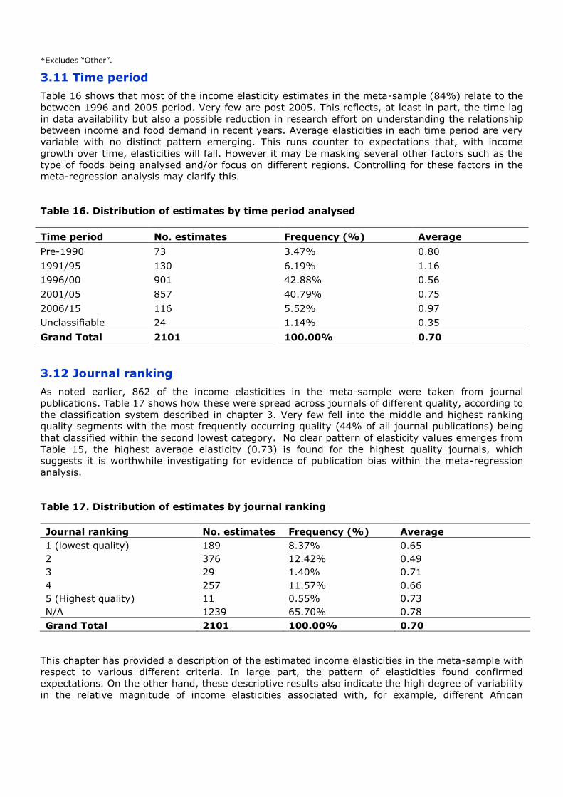
*Excludes “Other”.
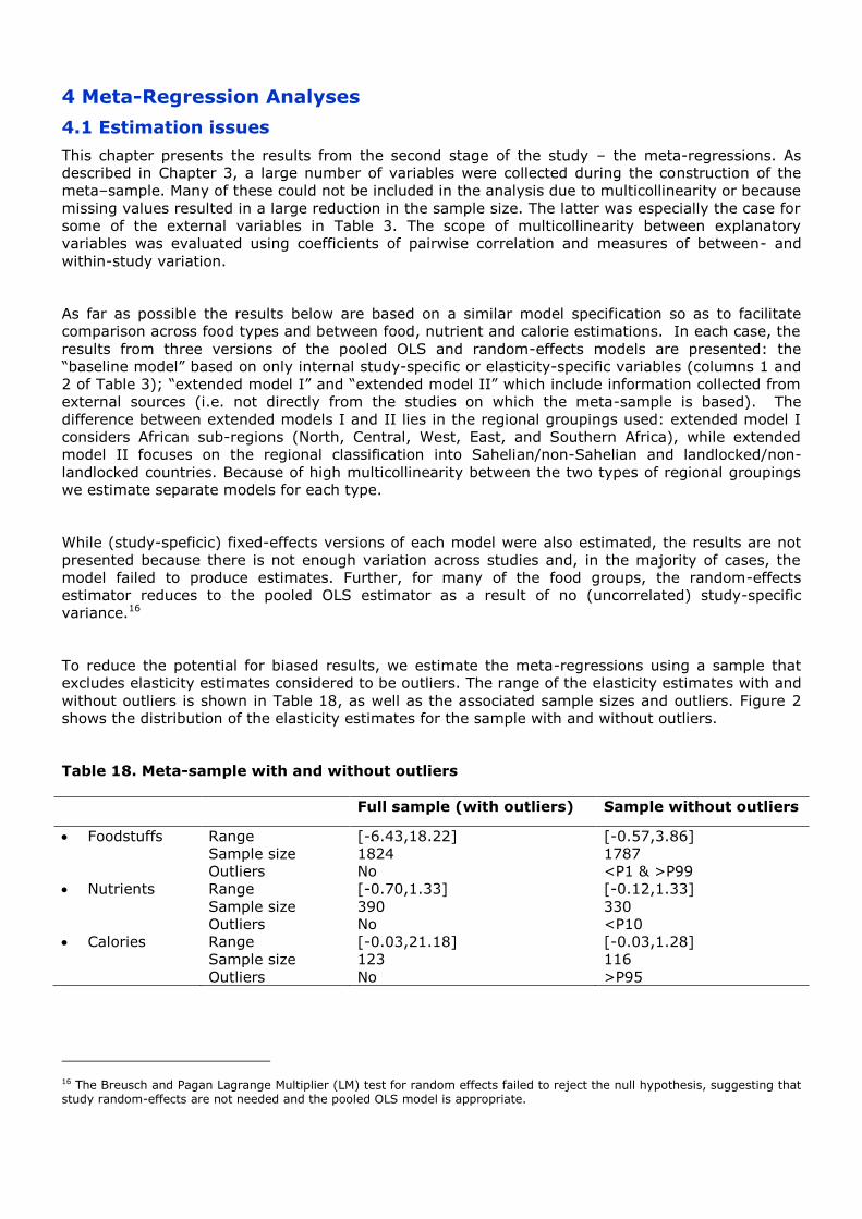
3.11 Time period
Table 16 shows that most of the income elasticity estimates in the meta-sample (84%) relate to the
between 1996 and 2005 period. Very few are post 2005. This reflects, at least in part, the time lag
in data availability but also a possible reduction in research effort on understanding the relationship
between income and food demand in recent years. Average elasticities in each time period are very
variable with no distinct pattern emerging. This runs counter to expectations that, with income
growth over time, elasticities will fall. However it may be masking several other factors such as the
type of foods being analysed and/or focus on different regions. Controlling for these factors in the
meta-regression analysis may clarify this.
Table 16. Distribution of estimates by time period analysed
Time period No. estimates Frequency (%) Average
Pre-1990 73 3.47% 0.80
1991/95 130 6.19% 1.16
1996/00 901 42.88% 0.56
2001/05 857 40.79% 0.75
2006/15 116 5.52% 0.97
Unclassifiable 24 1.14% 0.35
Grand Total 2101 100.00% 0.70
3.12 Journal ranking
As noted earlier, 862 of the income elasticities in the meta-sample were taken from journal
publications. Table 17 shows how these were spread across journals of different quality, according to
the classification system described in chapter 3. Very few fell into the middle and highest ranking
quality segments with the most frequently occurring quality (44% of all journal publications) being
that classified within the second lowest category. No clear pattern of elasticity values emerges from
Table 15, the highest average elasticity (0.73) is found for the highest quality journals, which
suggests it is worthwhile investigating for evidence of publication bias within the meta-regression
analysis.
Table 17. Distribution of estimates by journal ranking
Journal ranking No. estimates Frequency (%) Average
1 (lowest quality) 189 8.37% 0.65
2 376 12.42% 0.49
3 29 1.40% 0.71
4 257 11.57% 0.66
5 (Highest quality) 11 0.55% 0.73
N/A 1239 65.70% 0.78
Grand Total 2101 100.00% 0.70
This chapter has provided a description of the estimated income elasticities in the meta-sample with
respect to various different criteria. In large part, the pattern of elasticities found confirmed
expectations. On the other hand, these descriptive results also indicate the high degree of variability
in the relative magnitude of income elasticities associated with, for example, different African

countries and different household income groups. The next chapter explains how these findings were
used to inform the meta-regression stage of analysis.
4 Meta-Regression Analyses
4.1 Estimation issues
This chapter presents the results from the second stage of the study – the meta-regressions. As
described in Chapter 3, a large number of variables were collected during the construction of the
meta–sample. Many of these could not be included in the analysis due to multicollinearity or because
missing values resulted in a large reduction in the sample size. The latter was especially the case for
some of the external variables in Table 3. The scope of multicollinearity between explanatory
variables was evaluated using coefficients of pairwise correlation and measures of between- and
within-study variation.
As far as possible the results below are based on a similar model specification so as to facilitate
comparison across food types and between food, nutrient and calorie estimations. In each case, the
results from three versions of the pooled OLS and random-effects models are presented: the
“baseline model” based on only internal study-specific or elasticity-specific variables (columns 1 and
2 of Table 3); “extended model I” and “extended model II” which include information collected from
external sources (i.e. not directly from the studies on which the meta-sample is based). The
difference between extended models I and II lies in the regional groupings used: extended model I
considers African sub-regions (North, Central, West, East, and Southern Africa), while extended
model II focuses on the regional classification into Sahelian/non-Sahelian and landlocked/non-
landlocked countries. Because of high multicollinearity between the two types of regional groupings
we estimate separate models for each type.
While (study-speficic) fixed-effects versions of each model were also estimated, the results are not
presented because there is not enough variation across studies and, in the majority of cases, the
model failed to produce estimates. Further, for many of the food groups, the random-effects
estimator reduces to the pooled OLS estimator as a result of no (uncorrelated) study-specific
variance.16
To reduce the potential for biased results, we estimate the meta-regressions using a sample that
excludes elasticity estimates considered to be outliers. The range of the elasticity estimates with and
without outliers is shown in Table 18, as well as the associated sample sizes and outliers. Figure 2
shows the distribution of the elasticity estimates for the sample with and without outliers.
Table 18. Meta-sample with and without outliers
Full sample (with outliers) Sample without outliers
Foodstuffs Range
Sample size
Outliers
[-6.43,18.22]
1824
No
[-0.57,3.86]
1787
<P1 & >P99
Nutrients Range
Sample size
Outliers
[-0.70,1.33]
390
No
[-0.12,1.33]
330
<P10
Calories Range
Sample size
Outliers
[-0.03,21.18]
123
No
[-0.03,1.28]
116
>P95
16 The Breusch and Pagan Lagrange Multiplier (LM) test for random effects failed to reject the null hypothesis, suggesting that study random-effects are not needed and the pooled OLS model is appropriate.
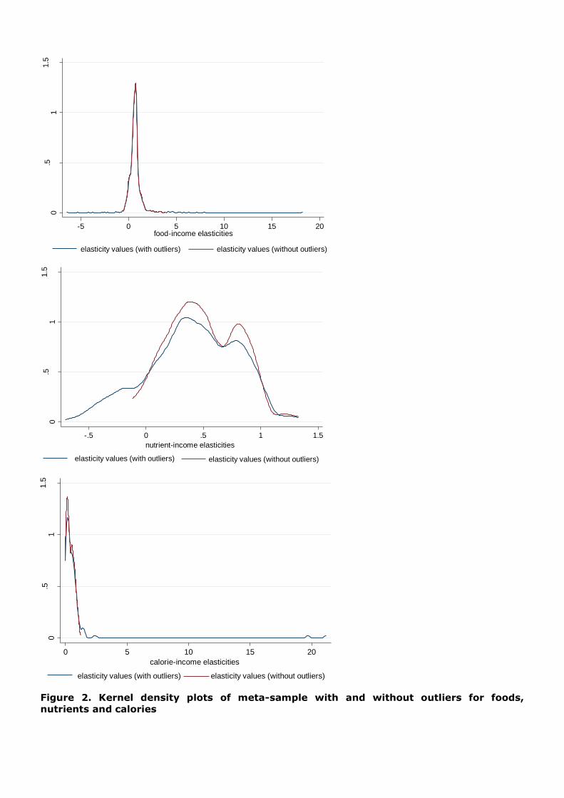
Figure 2. Kernel density plots of meta-sample with and without outliers for foods,
nutrients and calories
0.5
11.5
kdensity
-5 0 5 10 15 20food-income elasticities
elasticity values (with outliers) elasticity values (without outliers)
0.5
11.5
kdensity
-.5 0 .5 1 1.5
nutrient-income elasticities
elasticity values (with outliers) elasticity values (without outliers)
0.5
11.5
kdensity
0 5 10 15 20
calorie-income elasticities
elasticity values (with outliers) elasticity values (without outliers)
We estimate meta-regressions for foods (section 4.2.), nutrients (section 4.3.), and calories (section
4.4). In all cases, the coefficients of the meta-regressions measure the deviation (in percentage
points) from the elasticity value predicted by the models.
4.2 Foods
4.2.1 All foods
Table 19 presents the results for all foods pooled together. The baseline model uses 1,768 estimates
of income elasticities from 37 studies, while the extended models use 1,754 estimates of income
elasticities from 34 studies. Although the magnitude of some of the coefficients differ, qualitatively
the baseline and extended versions of the model produce similar results. Extending the model to
include country-specific external variables leads only to a marginal increase in the models’
explanatory power. Between-study variation contributes more to the explanatory power of the
models than within-study variation, which is in line with our expectations since differences across
elasticity estimates are likely to be larger between rather than within studies.
The bullet points below provide a summary of the main findings:
Working papers have significantly higher income elasticities compared to peer reviewed
journal studies. On the other hand, there is no clear difference between income elasticities
obtained from international organisations (i.e. reports) and peer reviewed journals.
Food demand is more responsive to changes in income for beverages, meat, fish and eggs,
compared to foods that tend to constitute basic diets (e.g. cereals, legumes and nuts, fruit
and vegetables and fats and oils, tubers). The trends across food groups are generally in line
with our expectations and reflect the nature of demand for stable products versus more
luxury food items.
Time series studies appear to produce significantly lower estimates than cross sectional and
panel data studies, after controlling for other study and estimate attributes, and external
variables.
In relation to the separate time periods, the period between 1996 and 2005 was a period of
income growth across Africa. The finding that elasticities estimated during this period are
significantly lower than those estimated for the early 1990s in the baseline model is therefore
as expected. However, there is no evidence that the trend of decreasing elasticities has
continued after 2005.
The coefficient on the GDP per capita variable suggests that as income increases the income
elasticity of demand for food falls: demands becomes less responsive to changes in income.
Again as expected, studies focusing on urban populations find significantly lower elasticities
than those looking at rural populations, or rural and urban populations jointly, even after
having controlled for the other study, elasticity and country attributes.
In line with other studies (Strauss and Thomas (1990) and Ogundari and Abdulai (2013)),
estimated elsticities are lower when using household expenditures as a proxy for income.
The type of demand model (single equation versus demand system) produced limited
differences. However, the type of estimator used appears to significantly affect the income
elasticity estimates although the direction of influence is inconclusive. For example, the
baseline model suggests LS and ML methods significantly estimate higher elasticities than IV
methods whilst the extended models suggest the opposite.
Income elasticities of demand for food in countries with greater degree of urbanisation are
lower. This conforms with our expectations.
There is some evidence of differences in the magnitude of food demand elasticities across the
sub-regions of Africa. On average, the income elasticity is higher for countries in Central
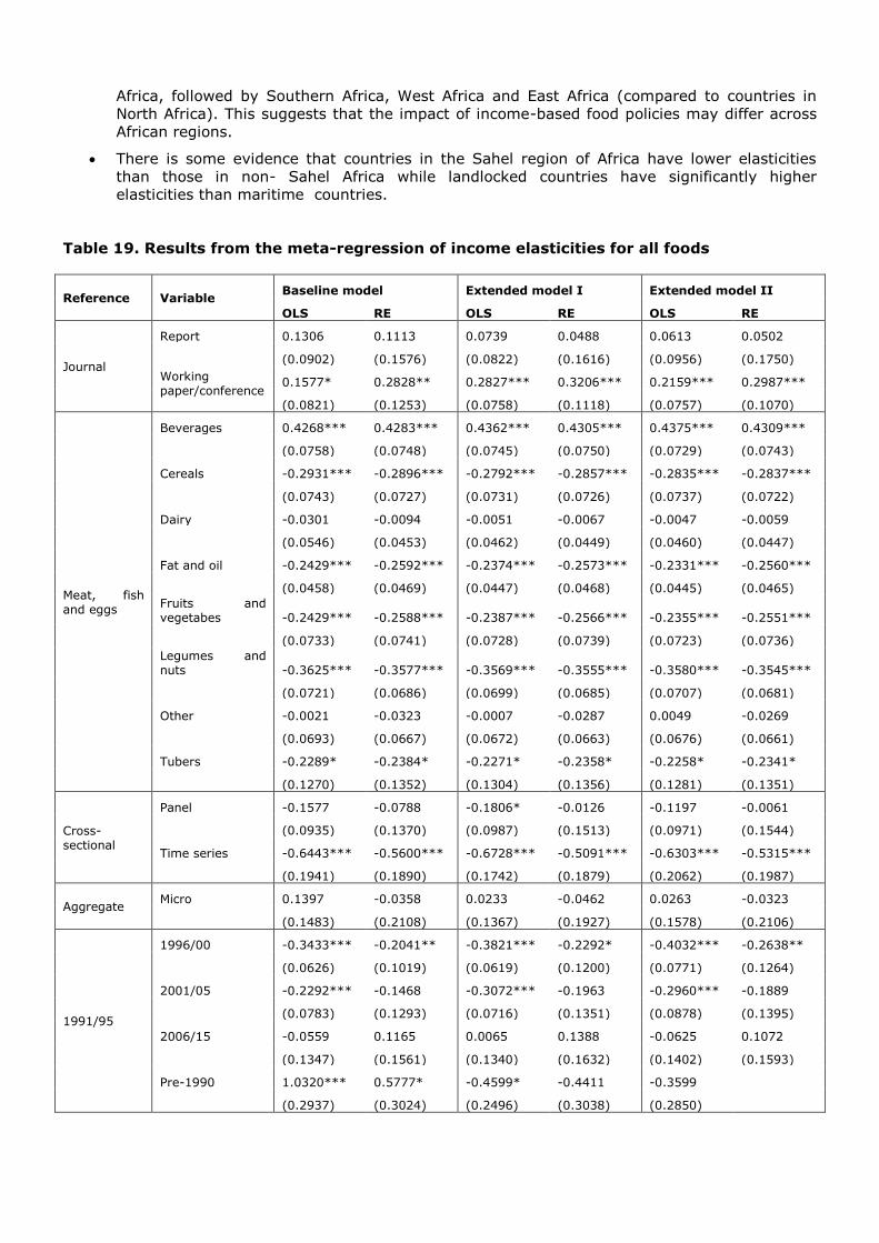
Africa, followed by Southern Africa, West Africa and East Africa (compared to countries in
North Africa). This suggests that the impact of income-based food policies may differ across
African regions.
There is some evidence that countries in the Sahel region of Africa have lower elasticities
than those in non- Sahel Africa while landlocked countries have significantly higher
elasticities than maritime countries.
Table 19. Results from the meta-regression of income elasticities for all foods
Reference Variable Baseline model Extended model I Extended model II
OLS RE OLS RE OLS RE
Journal
Report 0.1306 0.1113 0.0739 0.0488 0.0613 0.0502
(0.0902) (0.1576) (0.0822) (0.1616) (0.0956) (0.1750)
Working paper/conference
0.1577* 0.2828** 0.2827*** 0.3206*** 0.2159*** 0.2987***
(0.0821) (0.1253) (0.0758) (0.1118) (0.0757) (0.1070)
Meat, fish and eggs
Beverages 0.4268*** 0.4283*** 0.4362*** 0.4305*** 0.4375*** 0.4309***
(0.0758) (0.0748) (0.0745) (0.0750) (0.0729) (0.0743)
Cereals -0.2931*** -0.2896*** -0.2792*** -0.2857*** -0.2835*** -0.2837***
(0.0743) (0.0727) (0.0731) (0.0726) (0.0737) (0.0722)
Dairy -0.0301 -0.0094 -0.0051 -0.0067 -0.0047 -0.0059
(0.0546) (0.0453) (0.0462) (0.0449) (0.0460) (0.0447)
Fat and oil -0.2429*** -0.2592*** -0.2374*** -0.2573*** -0.2331*** -0.2560***
(0.0458) (0.0469) (0.0447) (0.0468) (0.0445) (0.0465)
Fruits and vegetabes -0.2429*** -0.2588*** -0.2387*** -0.2566*** -0.2355*** -0.2551***
(0.0733) (0.0741) (0.0728) (0.0739) (0.0723) (0.0736)
Legumes and nuts -0.3625*** -0.3577*** -0.3569*** -0.3555*** -0.3580*** -0.3545***
(0.0721) (0.0686) (0.0699) (0.0685) (0.0707) (0.0681)
Other -0.0021 -0.0323 -0.0007 -0.0287 0.0049 -0.0269
(0.0693) (0.0667) (0.0672) (0.0663) (0.0676) (0.0661)
Tubers -0.2289* -0.2384* -0.2271* -0.2358* -0.2258* -0.2341*
(0.1270) (0.1352) (0.1304) (0.1356) (0.1281) (0.1351)
Cross-sectional
Panel -0.1577 -0.0788 -0.1806* -0.0126 -0.1197 -0.0061
(0.0935) (0.1370) (0.0987) (0.1513) (0.0971) (0.1544)
Time series -0.6443*** -0.5600*** -0.6728*** -0.5091*** -0.6303*** -0.5315***
(0.1941) (0.1890) (0.1742) (0.1879) (0.2062) (0.1987)
Aggregate Micro 0.1397 -0.0358 0.0233 -0.0462 0.0263 -0.0323
(0.1483) (0.2108) (0.1367) (0.1927) (0.1578) (0.2106)
1991/95
1996/00 -0.3433*** -0.2041** -0.3821*** -0.2292* -0.4032*** -0.2638**
(0.0626) (0.1019) (0.0619) (0.1200) (0.0771) (0.1264)
2001/05 -0.2292*** -0.1468 -0.3072*** -0.1963 -0.2960*** -0.1889
(0.0783) (0.1293) (0.0716) (0.1351) (0.0878) (0.1395)
2006/15 -0.0559 0.1165 0.0065 0.1388 -0.0625 0.1072
(0.1347) (0.1561) (0.1340) (0.1632) (0.1402) (0.1593)
Pre-1990 1.0320*** 0.5777* -0.4599* -0.4411 -0.3599
(0.2937) (0.3024) (0.2496) (0.3038) (0.2850)
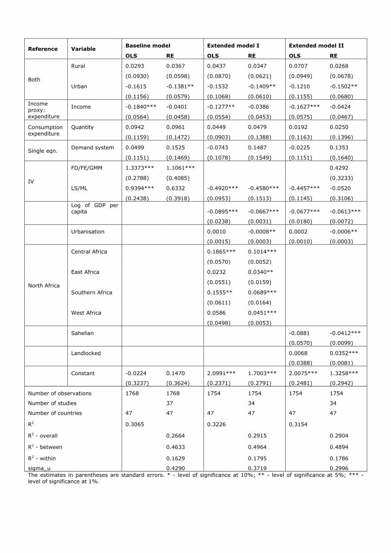
Reference Variable Baseline model Extended model I Extended model II
OLS RE OLS RE OLS RE
Both
Rural 0.0293 0.0367 0.0437 0.0347 0.0707 0.0268
(0.0930) (0.0598) (0.0870) (0.0621) (0.0949) (0.0678)
Urban -0.1615 -0.1381** -0.1532 -0.1409** -0.1210 -0.1502**
(0.1156) (0.0579) (0.1068) (0.0610) (0.1155) (0.0680)
Income proxy: expenditure
Income -0.1840*** -0.0401 -0.1277** -0.0386 -0.1627*** -0.0424
(0.0564) (0.0458) (0.0554) (0.0453) (0.0575) (0.0467)
Consumption expenditure
Quantity 0.0942 0.0961 0.0449 0.0479 0.0192 0.0250
(0.1159) (0.1472) (0.0903) (0.1388) (0.1163) (0.1396)
Single eqn. Demand system 0.0499 0.1525 -0.0743 0.1487 -0.0225 0.1353
(0.1151) (0.1469) (0.1078) (0.1549) (0.1151) (0.1640)
IV
FD/FE/GMM 1.3373*** 1.1061*** 0.4292
(0.2788) (0.4085)
(0.3233)
LS/ML 0.9394*** 0.6332 -0.4920*** -0.4580*** -0.4457*** -0.0520
(0.2438) (0.3918) (0.0953) (0.1513) (0.1145) (0.3106)
Log of GDP per capita -0.0895*** -0.0667*** -0.0677*** -0.0613***
(0.0238) (0.0031) (0.0180) (0.0072)
Urbanisation 0.0010 -0.0008** 0.0002 -0.0006**
(0.0015) (0.0003) (0.0010) (0.0003)
North Africa
Central Africa 0.1865*** 0.1014***
(0.0570) (0.0052)
East Africa
0.0232 0.0340**
(0.0551) (0.0159)
Southern Africa
0.1555** 0.0689***
(0.0611) (0.0164)
West Africa
0.0586 0.0451***
(0.0498) (0.0053)
Sahelian -0.0881 -0.0412***
(0.0570) (0.0099)
Landlocked 0.0068 0.0352***
(0.0388) (0.0081)
Constant -0.0224 0.1470 2.0991*** 1.7003*** 2.0075*** 1.3258***
(0.3237) (0.3624) (0.2371) (0.2791) (0.2481) (0.2942)
Number of observations 1768 1768 1754 1754 1754 1754
Number of studies
37
34
34
Number of countries 47 47 47 47 47 47
R2 0.3065
0.3226
0.3154
R2 - overall
0.2664
0.2915
0.2904
R2 - between
0.4633
0.4964
0.4894
R2 - within
0.1629
0.1795
0.1786
sigma_u 0.4290 0.3719 0.2996
The estimates in parentheses are standard errors. * - level of significance at 10%; ** - level of significance at 5%; *** - level of significance at 1%.
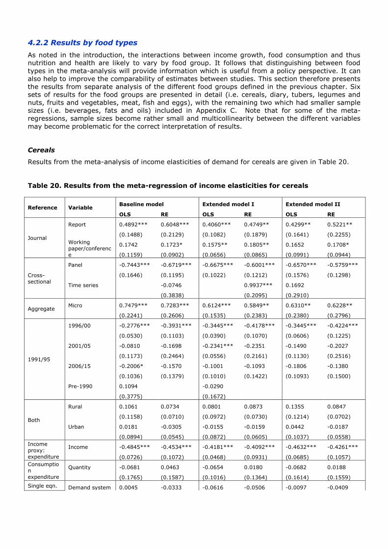
4.2.2 Results by food types
As noted in the introduction, the interactions between income growth, food consumption and thus
nutrition and health are likely to vary by food group. It follows that distinguishing between food
types in the meta-analysis will provide information which is useful from a policy perspective. It can
also help to improve the comparability of estimates between studies. This section therefore presents
the results from separate analysis of the different food groups defined in the previous chapter. Six
sets of results for the food groups are presented in detail (i.e. cereals, diary, tubers, legumes and
nuts, fruits and vegetables, meat, fish and eggs), with the remaining two which had smaller sample
sizes (i.e. beverages, fats and oils) included in Appendix C. Note that for some of the meta-
regressions, sample sizes become rather small and multicollinearity between the different variables
may become problematic for the correct interpretation of results.
Cereals
Results from the meta-analysis of income elasticities of demand for cereals are given in Table 20.
Table 20. Results from the meta-regression of income elasticities for cereals
Reference Variable Baseline model Extended model I Extended model II
OLS RE OLS RE OLS RE
Journal
Report 0.4892*** 0.6048*** 0.4060*** 0.4749** 0.4299** 0.5221**
(0.1488) (0.2129) (0.1082) (0.1879) (0.1641) (0.2255)
Working paper/conference
0.1742 0.1723* 0.1575** 0.1805** 0.1652 0.1708*
(0.1159) (0.0902) (0.0656) (0.0865) (0.0991) (0.0944)
Cross-sectional
Panel -0.7443*** -0.6719*** -0.6675*** -0.6001*** -0.6570*** -0.5759***
(0.1646) (0.1195) (0.1022) (0.1212) (0.1576) (0.1298)
Time series -0.0746 0.9937*** 0.1692
(0.3838) (0.2095) (0.2910)
Aggregate Micro 0.7479*** 0.7283*** 0.6124*** 0.5849** 0.6310** 0.6228**
(0.2241) (0.2606) (0.1535) (0.2383) (0.2380) (0.2796)
1991/95
1996/00 -0.2776*** -0.3931*** -0.3445*** -0.4178*** -0.3445*** -0.4224***
(0.0530) (0.1103) (0.0390) (0.1070) (0.0606) (0.1225)
2001/05 -0.0810 -0.1698 -0.2341*** -0.2351 -0.1490 -0.2027
(0.1173) (0.2464) (0.0556) (0.2161) (0.1130) (0.2516)
2006/15 -0.2006* -0.1570 -0.1001 -0.1093 -0.1806 -0.1380
(0.1036) (0.1379) (0.1010) (0.1422) (0.1093) (0.1500)
Pre-1990 0.1094 -0.0290
(0.3775) (0.1672)
Both
Rural 0.1061 0.0734 0.0801 0.0873 0.1355 0.0847
(0.1158) (0.0710) (0.0972) (0.0730) (0.1214) (0.0702)
Urban 0.0181 -0.0305 -0.0155 -0.0159 0.0442 -0.0187
(0.0894) (0.0545) (0.0872) (0.0605) (0.1037) (0.0558)
Income proxy: expenditure
Income -0.4845*** -0.4534*** -0.4181*** -0.4092*** -0.4632*** -0.4261***
(0.0726) (0.1072) (0.0468) (0.0931) (0.0685) (0.1057)
Consumption expenditure
Quantity -0.0681 0.0463 -0.0654 0.0180 -0.0682 0.0188
(0.1765) (0.1587) (0.1016) (0.1364) (0.1614) (0.1559)
Single eqn. Demand system 0.0045 -0.0333 -0.0616 -0.0506 -0.0097 -0.0409
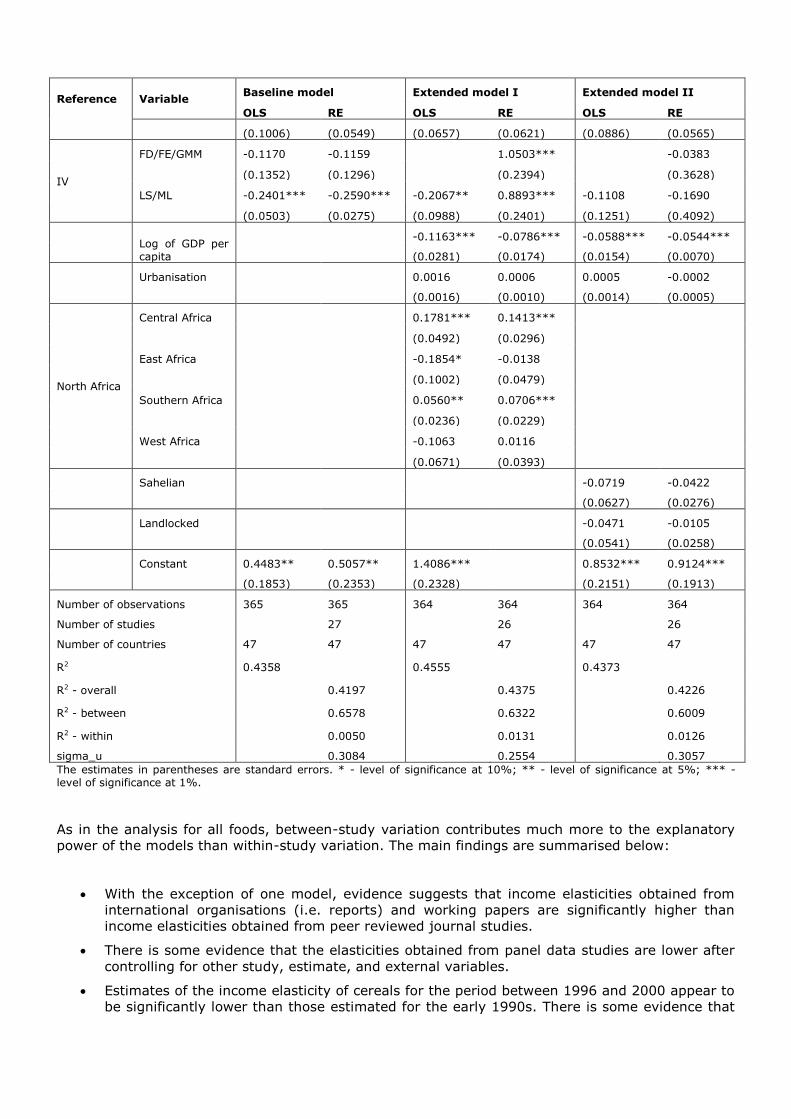
Reference Variable Baseline model Extended model I Extended model II
OLS RE OLS RE OLS RE
(0.1006) (0.0549) (0.0657) (0.0621) (0.0886) (0.0565)
IV
FD/FE/GMM -0.1170 -0.1159 1.0503***
-0.0383
(0.1352) (0.1296) (0.2394)
(0.3628)
LS/ML -0.2401*** -0.2590*** -0.2067** 0.8893*** -0.1108 -0.1690
(0.0503) (0.0275) (0.0988) (0.2401) (0.1251) (0.4092)
Log of GDP per capita
-0.1163*** -0.0786*** -0.0588*** -0.0544***
(0.0281) (0.0174) (0.0154) (0.0070)
Urbanisation 0.0016 0.0006 0.0005 -0.0002
(0.0016) (0.0010) (0.0014) (0.0005)
North Africa
Central Africa 0.1781*** 0.1413***
(0.0492) (0.0296)
East Africa -0.1854* -0.0138
(0.1002) (0.0479)
Southern Africa 0.0560** 0.0706***
(0.0236) (0.0229)
West Africa -0.1063 0.0116
(0.0671) (0.0393)
Sahelian -0.0719 -0.0422
(0.0627) (0.0276)
Landlocked -0.0471 -0.0105
(0.0541) (0.0258)
Constant 0.4483** 0.5057** 1.4086*** 0.8532*** 0.9124***
(0.1853) (0.2353) (0.2328) (0.2151) (0.1913)
Number of observations 365 365 364 364 364 364
Number of studies 27 26
26
Number of countries 47 47 47 47 47 47
R2 0.4358 0.4555 0.4373
R2 - overall 0.4197 0.4375
0.4226
R2 - between 0.6578 0.6322
0.6009
R2 - within 0.0050 0.0131
0.0126
sigma_u 0.3084 0.2554 0.3057
The estimates in parentheses are standard errors. * - level of significance at 10%; ** - level of significance at 5%; *** - level of significance at 1%.
As in the analysis for all foods, between-study variation contributes much more to the explanatory
power of the models than within-study variation. The main findings are summarised below:
With the exception of one model, evidence suggests that income elasticities obtained from
international organisations (i.e. reports) and working papers are significantly higher than
income elasticities obtained from peer reviewed journal studies.
There is some evidence that the elasticities obtained from panel data studies are lower after
controlling for other study, estimate, and external variables.
Estimates of the income elasticity of cereals for the period between 1996 and 2000 appear to
be significantly lower than those estimated for the early 1990s. There is some evidence that
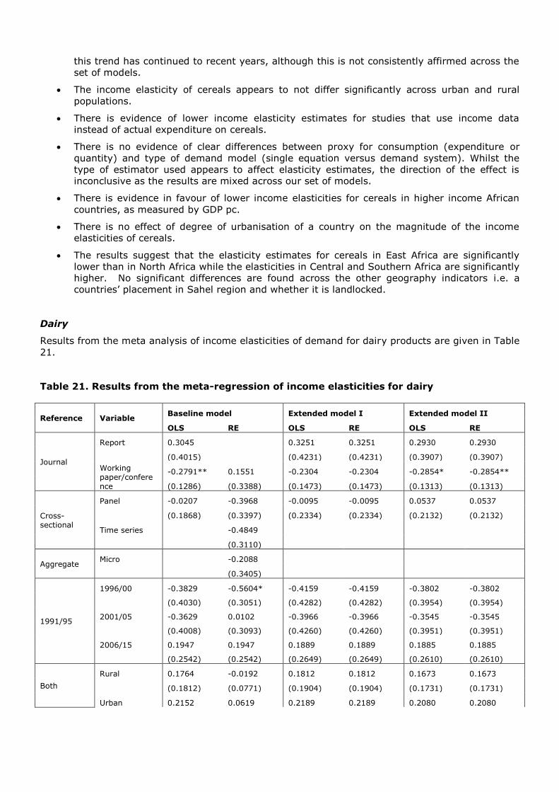
this trend has continued to recent years, although this is not consistently affirmed across the
set of models.
The income elasticity of cereals appears to not differ significantly across urban and rural
populations.
There is evidence of lower income elasticity estimates for studies that use income data
instead of actual expenditure on cereals.
There is no evidence of clear differences between proxy for consumption (expenditure or
quantity) and type of demand model (single equation versus demand system). Whilst the
type of estimator used appears to affect elasticity estimates, the direction of the effect is
inconclusive as the results are mixed across our set of models.
There is evidence in favour of lower income elasticities for cereals in higher income African
countries, as measured by GDP pc.
There is no effect of degree of urbanisation of a country on the magnitude of the income
elasticities of cereals.
The results suggest that the elasticity estimates for cereals in East Africa are significantly
lower than in North Africa while the elasticities in Central and Southern Africa are significantly
higher. No significant differences are found across the other geography indicators i.e. a
countries’ placement in Sahel region and whether it is landlocked.
Dairy
Results from the meta analysis of income elasticities of demand for dairy products are given in Table
21.
Table 21. Results from the meta-regression of income elasticities for dairy
Reference Variable Baseline model Extended model I Extended model II
OLS RE OLS RE OLS RE
Journal
Report 0.3045 0.3251 0.3251 0.2930 0.2930
(0.4015) (0.4231) (0.4231) (0.3907) (0.3907)
Working paper/conference
-0.2791** 0.1551 -0.2304 -0.2304 -0.2854* -0.2854**
(0.1286) (0.3388) (0.1473) (0.1473) (0.1313) (0.1313)
Cross-sectional
Panel -0.0207 -0.3968 -0.0095 -0.0095 0.0537 0.0537
(0.1868) (0.3397) (0.2334) (0.2334) (0.2132) (0.2132)
Time series -0.4849
(0.3110)
Aggregate Micro -0.2088
(0.3405)
1991/95
1996/00 -0.3829 -0.5604* -0.4159 -0.4159 -0.3802 -0.3802
(0.4030) (0.3051) (0.4282) (0.4282) (0.3954) (0.3954)
2001/05 -0.3629 0.0102 -0.3966 -0.3966 -0.3545 -0.3545
(0.4008) (0.3093) (0.4260) (0.4260) (0.3951) (0.3951)
2006/15 0.1947 0.1947 0.1889 0.1889 0.1885 0.1885
(0.2542) (0.2542) (0.2649) (0.2649) (0.2610) (0.2610)
Both
Rural 0.1764 -0.0192 0.1812 0.1812 0.1673 0.1673
(0.1812) (0.0771) (0.1904) (0.1904) (0.1731) (0.1731)
Urban 0.2152 0.0619 0.2189 0.2189 0.2080 0.2080
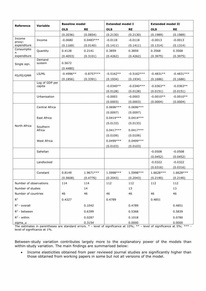
Reference Variable Baseline model Extended model I Extended model II
OLS RE OLS RE OLS RE
(0.2036) (0.0854) (0.2130) (0.2130) (0.1989) (0.1989)
Income proxy: expenditure
Income -0.0680 0.0483*** -0.0118 -0.0118 -0.0013 -0.0013
(0.1169) (0.0140) (0.1411) (0.1411) (0.1314) (0.1314)
Consumption expenditure
Quantity 0.4128 0.2141 0.3859 0.3859 0.3568 0.3568
(0.4053) (0.3101) (0.4262) (0.4262) (0.3975) (0.3975)
Single eqn.
Demand system 0.5672
(0.4480)
FD/FE/GMM LS/ML -0.4996** -0.8757*** -0.5162** -0.5162*** -0.4831** -0.4831***
(0.1856) (0.3391) (0.1934) (0.1934) (0.1686) (0.1686)
Log of GDP per capita -0.0340** -0.0340*** -0.0363** -0.0363**
(0.0128) (0.0128) (0.0151) (0.0151)
Urbanisation -0.0003 -0.0003 -0.0010** -0.0010**
(0.0003) (0.0003) (0.0004) (0.0004)
North Africa
Central Africa 0.0696*** 0.0696***
(0.0097) (0.0097)
East Africa 0.0414*** 0.0414***
(0.0133) (0.0133)
Southern Africa 0.0417*** 0.0417***
(0.0109) (0.0109)
West Africa 0.0499*** 0.0499***
(0.0103) (0.0103)
Sahelian -0.0508 -0.0508
(0.0452) (0.0452)
Landlocked -0.0322 -0.0322
(0.0316) (0.0316)
Constant 0.8149 1.9671*** 1.5998*** 1.5998*** 1.6628*** 1.6628***
(0.5608) (0.4776) (0.2043) (0.2043) (0.2190) (0.2190)
Number of observations 114 114 112 112 112 112
Number of studies 14 13
13
Number of countries 46 46 46 46 46 46
R2 0.4327 0.4789 0.4851
R2 - overall 0.1042 0.4789
0.4851
R2 - between 0.6399 0.5368
0.5839
R2 - within 0.0287 0.1018
0.0780
sigma_u 0.3154 0.0000 0.0000
The estimates in parentheses are standard errors. * - level of significance at 10%; ** - level of significance at 5%; *** - level of significance at 1%.
Between-study variation contributes largely more to the explanatory power of the models than
within-study variation. The main findings are summarised below:
Income elasticities obtained from peer reviewed journal studies are significantly higher than
those obtained from working papers in some but not all versions of the model.
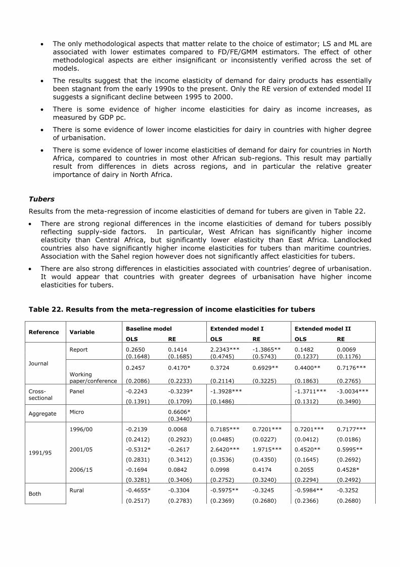
The only methodological aspects that matter relate to the choice of estimator; LS and ML are
associated with lower estimates compared to FD/FE/GMM estimators. The effect of other
methodological aspects are either insignificant or inconsistently verified across the set of
models.
The results suggest that the income elasticity of demand for dairy products has essentially
been stagnant from the early 1990s to the present. Only the RE version of extended model II
suggests a significant decline between 1995 to 2000.
There is some evidence of higher income elasticities for dairy as income increases, as
measured by GDP pc.
There is some evidence of lower income elasticities for dairy in countries with higher degree
of urbanisation.
There is some evidence of lower income elasticities of demand for dairy for countries in North
Africa, compared to countries in most other African sub-regions. This result may partially
result from differences in diets across regions, and in particular the relative greater
importance of dairy in North Africa.
Tubers
Results from the meta-regression of income elasticities of demand for tubers are given in Table 22.
There are strong regional differences in the income elasticities of demand for tubers possibly
reflecting supply-side factors. In particular, West African has significantly higher income
elasticity than Central Africa, but significantly lower elasticity than East Africa. Landlocked
countries also have significantly higher income elasticities for tubers than maritime countries.
Association with the Sahel region however does not significantly affect elasticities for tubers.
There are also strong differences in elasticities associated with countries’ degree of urbanisation.
It would appear that countries with greater degrees of urbanisation have higher income
elasticities for tubers.
Table 22. Results from the meta-regression of income elasticities for tubers
Reference Variable Baseline model Extended model I Extended model II
OLS RE OLS RE OLS RE
Journal
Report 0.2650 0.1414 2.2343*** -1.3865** 0.1482 0.0069
(0.1648) (0.1685) (0.4745) (0.5743) (0.1237) (0.1176)
Working paper/conference
0.2457 0.4170* 0.3724 0.6929** 0.4400** 0.7176***
(0.2086) (0.2233) (0.2114) (0.3225) (0.1863) (0.2765)
Cross-sectional
Panel -0.2243 -0.3239* -1.3928*** -1.3711*** -3.0034***
(0.1391) (0.1709) (0.1486) (0.1312) (0.3490)
Aggregate Micro 0.6606*
(0.3440)
1991/95
1996/00 -0.2139 0.0068 0.7185*** 0.7201*** 0.7201*** 0.7177***
(0.2412) (0.2923) (0.0485) (0.0227) (0.0412) (0.0186)
2001/05 -0.5312* -0.2617 2.6420*** 1.9715*** 0.4520** 0.5995**
(0.2831) (0.3412) (0.3536) (0.4350) (0.1645) (0.2692)
2006/15 -0.1694 0.0842 0.0998 0.4174 0.2055 0.4528*
(0.3281) (0.3406) (0.2752) (0.3240) (0.2294) (0.2492)
Both Rural -0.4655* -0.3304 -0.5975** -0.3245 -0.5984** -0.3252
(0.2517) (0.2783) (0.2369) (0.2680) (0.2366) (0.2680)
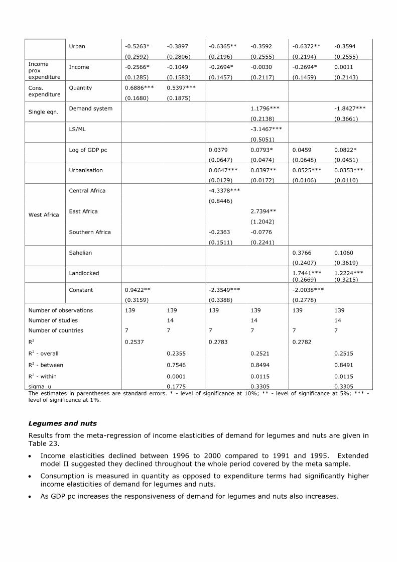
Urban -0.5263* -0.3897 -0.6365** -0.3592 -0.6372** -0.3594
(0.2592) (0.2806) (0.2196) (0.2555) (0.2194) (0.2555)
Income prox expenditure
Income -0.2566* -0.1049 -0.2694* -0.0030 -0.2694* 0.0011
(0.1285) (0.1583) (0.1457) (0.2117) (0.1459) (0.2143)
Cons. expenditure
Quantity 0.6886*** 0.5397***
(0.1680) (0.1875)
Single eqn. Demand system 1.1796*** -1.8427***
(0.2138) (0.3661)
LS/ML -3.1467***
(0.5051)
Log of GDP pc 0.0379 0.0793* 0.0459 0.0822*
(0.0647) (0.0474) (0.0648) (0.0451)
Urbanisation 0.0647*** 0.0397** 0.0525*** 0.0353***
(0.0129) (0.0172) (0.0106) (0.0110)
West Africa
Central Africa -4.3378***
(0.8446)
East Africa 2.7394**
(1.2042)
Southern Africa -0.2363 -0.0776
(0.1511) (0.2241)
Sahelian 0.3766 0.1060
(0.2407) (0.3619)
Landlocked 1.7441*** 1.2224*** (0.2669) (0.3215)
Constant 0.9422** -2.3549*** -2.0038***
(0.3159) (0.3388) (0.2778)
Number of observations 139 139 139 139 139 139
Number of studies 14 14 14
Number of countries 7 7 7 7 7 7
R2 0.2537 0.2783 0.2782
R2 - overall 0.2355 0.2521 0.2515
R2 - between 0.7546 0.8494 0.8491
R2 - within 0.0001 0.0115 0.0115
sigma_u 0.1775 0.3305 0.3305
The estimates in parentheses are standard errors. * - level of significance at 10%; ** - level of significance at 5%; *** - level of significance at 1%.
Legumes and nuts
Results from the meta-regression of income elasticities of demand for legumes and nuts are given in
Table 23.
Income elasticities declined between 1996 to 2000 compared to 1991 and 1995. Extended
model II suggested they declined throughout the whole period covered by the meta sample.
Consumption is measured in quantity as opposed to expenditure terms had significantly higher
income elasticities of demand for legumes and nuts.
As GDP pc increases the responsiveness of demand for legumes and nuts also increases.
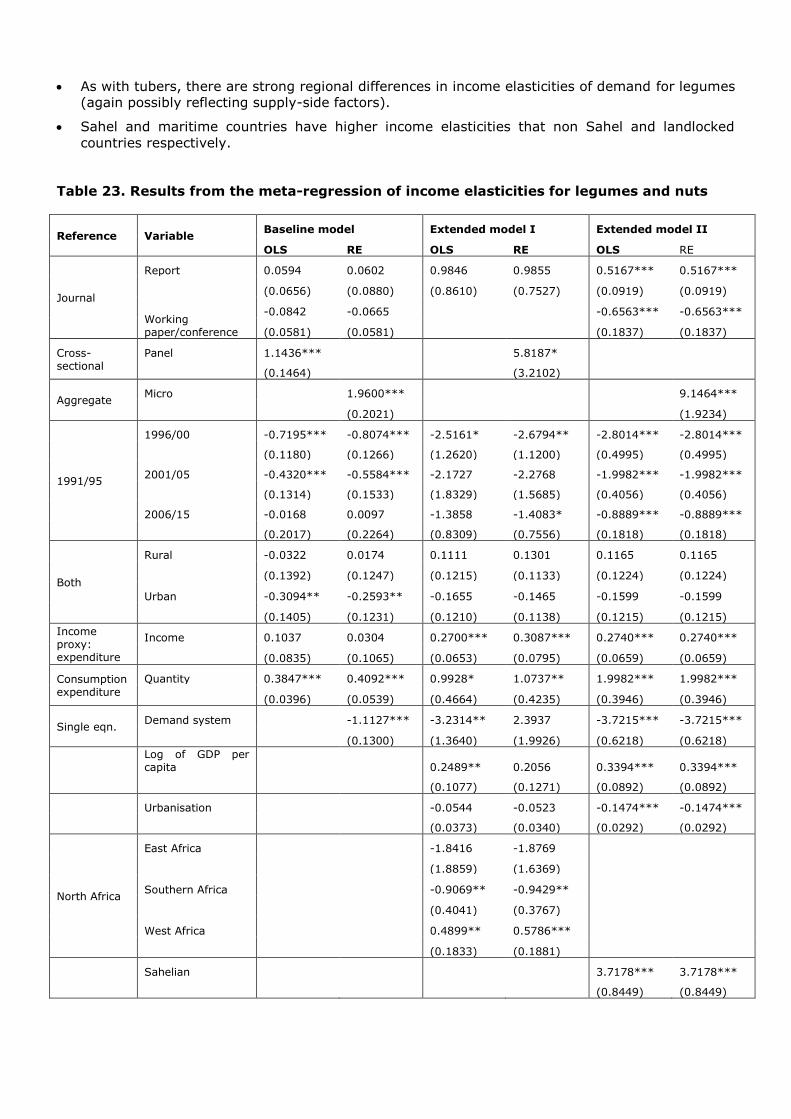
As with tubers, there are strong regional differences in income elasticities of demand for legumes
(again possibly reflecting supply-side factors).
Sahel and maritime countries have higher income elasticities that non Sahel and landlocked
countries respectively.
Table 23. Results from the meta-regression of income elasticities for legumes and nuts
Reference Variable Baseline model Extended model I Extended model II
OLS RE OLS RE OLS RE
Journal
Report 0.0594 0.0602 0.9846 0.9855 0.5167*** 0.5167***
(0.0656) (0.0880) (0.8610) (0.7527) (0.0919) (0.0919)
Working paper/conference
-0.0842 -0.0665 -0.6563*** -0.6563***
(0.0581) (0.0581) (0.1837) (0.1837)
Cross-sectional
Panel 1.1436*** 5.8187*
(0.1464) (3.2102)
Aggregate Micro 1.9600*** 9.1464***
(0.2021) (1.9234)
1991/95
1996/00 -0.7195*** -0.8074*** -2.5161* -2.6794** -2.8014*** -2.8014***
(0.1180) (0.1266) (1.2620) (1.1200) (0.4995) (0.4995)
2001/05 -0.4320*** -0.5584*** -2.1727 -2.2768 -1.9982*** -1.9982***
(0.1314) (0.1533) (1.8329) (1.5685) (0.4056) (0.4056)
2006/15 -0.0168 0.0097 -1.3858 -1.4083* -0.8889*** -0.8889***
(0.2017) (0.2264) (0.8309) (0.7556) (0.1818) (0.1818)
Both
Rural -0.0322 0.0174 0.1111 0.1301 0.1165 0.1165
(0.1392) (0.1247) (0.1215) (0.1133) (0.1224) (0.1224)
Urban -0.3094** -0.2593** -0.1655 -0.1465 -0.1599 -0.1599
(0.1405) (0.1231) (0.1210) (0.1138) (0.1215) (0.1215)
Income proxy: expenditure
Income 0.1037 0.0304 0.2700*** 0.3087*** 0.2740*** 0.2740***
(0.0835) (0.1065) (0.0653) (0.0795) (0.0659) (0.0659)
Consumption expenditure
Quantity 0.3847*** 0.4092*** 0.9928* 1.0737** 1.9982*** 1.9982***
(0.0396) (0.0539) (0.4664) (0.4235) (0.3946) (0.3946)
Single eqn. Demand system -1.1127*** -3.2314** 2.3937 -3.7215*** -3.7215***
(0.1300) (1.3640) (1.9926) (0.6218) (0.6218)
Log of GDP per capita 0.2489** 0.2056 0.3394*** 0.3394***
(0.1077) (0.1271) (0.0892) (0.0892)
Urbanisation -0.0544 -0.0523 -0.1474*** -0.1474***
(0.0373) (0.0340) (0.0292) (0.0292)
North Africa
East Africa -1.8416 -1.8769
(1.8859) (1.6369)
Southern Africa -0.9069** -0.9429**
(0.4041) (0.3767)
West Africa 0.4899** 0.5786***
(0.1833) (0.1881)
Sahelian 3.7178*** 3.7178***
(0.8449) (0.8449)
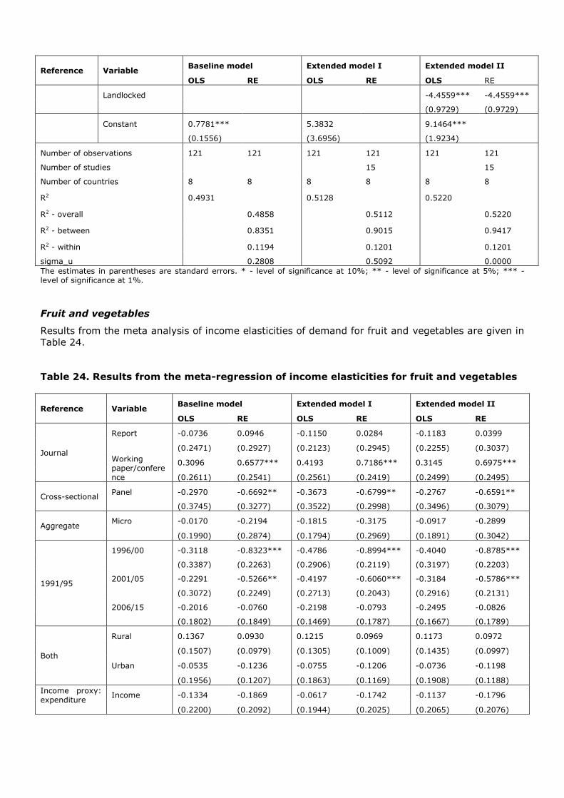
Reference Variable Baseline model Extended model I Extended model II
OLS RE OLS RE OLS RE
Landlocked -4.4559*** -4.4559***
(0.9729) (0.9729)
Constant 0.7781*** 5.3832 9.1464***
(0.1556) (3.6956) (1.9234)
Number of observations 121 121 121 121 121 121
Number of studies
15 15
Number of countries 8 8 8 8 8 8
R2 0.4931 0.5128 0.5220
R2 - overall 0.4858 0.5112 0.5220
R2 - between 0.8351 0.9015 0.9417
R2 - within 0.1194 0.1201 0.1201
sigma_u 0.2808 0.5092 0.0000
The estimates in parentheses are standard errors. * - level of significance at 10%; ** - level of significance at 5%; *** - level of significance at 1%.
Fruit and vegetables
Results from the meta analysis of income elasticities of demand for fruit and vegetables are given in
Table 24.
Table 24. Results from the meta-regression of income elasticities for fruit and vegetables
Reference Variable Baseline model Extended model I Extended model II
OLS RE OLS RE OLS RE
Journal
Report -0.0736 0.0946 -0.1150 0.0284 -0.1183 0.0399
(0.2471) (0.2927) (0.2123) (0.2945) (0.2255) (0.3037)
Working paper/conference
0.3096 0.6577*** 0.4193 0.7186*** 0.3145 0.6975***
(0.2611) (0.2541) (0.2561) (0.2419) (0.2499) (0.2495)
Cross-sectional Panel -0.2970 -0.6692** -0.3673 -0.6799** -0.2767 -0.6591**
(0.3745) (0.3277) (0.3522) (0.2998) (0.3496) (0.3079)
Aggregate Micro -0.0170 -0.2194 -0.1815 -0.3175 -0.0917 -0.2899
(0.1990) (0.2874) (0.1794) (0.2969) (0.1891) (0.3042)
1991/95
1996/00 -0.3118 -0.8323*** -0.4786 -0.8994*** -0.4040 -0.8785***
(0.3387) (0.2263) (0.2906) (0.2119) (0.3197) (0.2203)
2001/05 -0.2291 -0.5266** -0.4197 -0.6060*** -0.3184 -0.5786***
(0.3072) (0.2249) (0.2713) (0.2043) (0.2916) (0.2131)
2006/15 -0.2016 -0.0760 -0.2198 -0.0793 -0.2495 -0.0826
(0.1802) (0.1849) (0.1469) (0.1787) (0.1667) (0.1789)
Both
Rural 0.1367 0.0930 0.1215 0.0969 0.1173 0.0972
(0.1507) (0.0979) (0.1305) (0.1009) (0.1435) (0.0997)
Urban -0.0535 -0.1236 -0.0755 -0.1206 -0.0736 -0.1198
(0.1956) (0.1207) (0.1863) (0.1169) (0.1908) (0.1188)
Income proxy: expenditure
Income -0.1334 -0.1869 -0.0617 -0.1742 -0.1137 -0.1796
(0.2200) (0.2092) (0.1944) (0.2025) (0.2065) (0.2076)
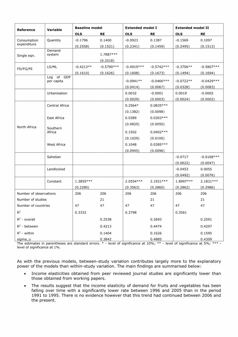
Reference Variable Baseline model Extended model I Extended model II
OLS RE OLS RE OLS RE
Consumption expenditure
Quantity -0.1796 0.1400 -0.0923 0.1387 -0.1569 0.1097
(0.2558) (0.1521) (0.2341) (0.1459) (0.2495) (0.1513)
Single eqn.
Demand system 1.7887***
(0.2518)
FD/FG/FE LS/ML -0.4213** -0.5790*** -0.4919*** -0.5742*** -0.3706** -0.5807***
(0.1610) (0.1626) (0.1608) (0.1673) (0.1494) (0.1694)
Log of GDP per capita -0.0941** -0.0466*** -0.0722** -0.0429***
(0.0414) (0.0067) (0.0328) (0.0083)
Urbanisation 0.0032 -0.0001 0.0019 -0.0002
(0.0029) (0.0003) (0.0024) (0.0002)
North Africa
Central Africa 0.2564* 0.0835***
(0.1382) (0.0098)
East Africa 0.0389 0.0303***
(0.0825) (0.0050)
Southern Africa 0.1502 0.0402***
(0.1029) (0.0100)
West Africa 0.1048 0.0385***
(0.0945) (0.0096)
Sahelian -0.0717 -0.0168***
(0.0622) (0.0047)
Landlocked -0.0453 0.0055
(0.0492) (0.0076)
Constant 1.3855*** 2.0554*** 2.1921*** 1.8997*** 2.1831***
(0.2280) (0.3563) (0.2860) (0.2862) (0.2986)
Number of observations 206 206 206 206 206 206
Number of studies 21 21
21
Number of countries 47 47 47 47 47 47
R2 0.3332 0.3798 0.3561
R2 - overall 0.2538 0.2693
0.2591
R2 - between 0.4213 0.4474
0.4297
R2 - within 0.1404 0.1626
0.1595
sigma_u 0.3842 0.4885 0.4309
The estimates in parentheses are standard errors. * - level of significance at 10%; ** - level of significance at 5%; *** - level of significance at 1%.
As with the previous models, between-study variation contributes largely more to the explanatory
power of the models than within-study variation. The main findings are summarised below:
Income elasticities obtained from peer reviewed journal studies are significantly lower than
those obtained from working papers.
The results suggest that the income elasticity of demand for fruits and vegetables has been
falling over time with a significantly lower rate between 1996 and 2005 than in the period
1991 to 1995. There is no evidence however that this trend had continued between 2006 and
the present.
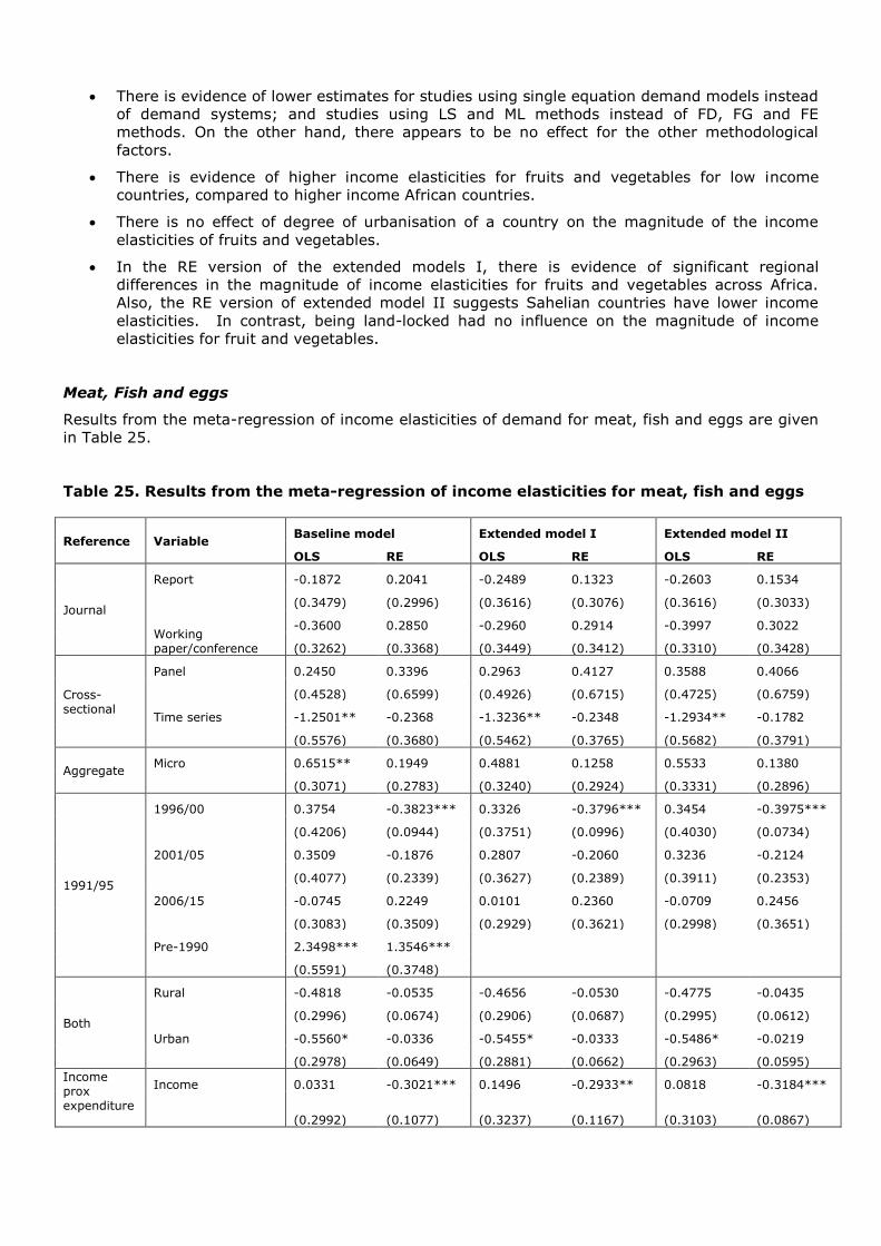
There is evidence of lower estimates for studies using single equation demand models instead
of demand systems; and studies using LS and ML methods instead of FD, FG and FE
methods. On the other hand, there appears to be no effect for the other methodological
factors.
There is evidence of higher income elasticities for fruits and vegetables for low income
countries, compared to higher income African countries.
There is no effect of degree of urbanisation of a country on the magnitude of the income
elasticities of fruits and vegetables.
In the RE version of the extended models I, there is evidence of significant regional
differences in the magnitude of income elasticities for fruits and vegetables across Africa.
Also, the RE version of extended model II suggests Sahelian countries have lower income
elasticities. In contrast, being land-locked had no influence on the magnitude of income
elasticities for fruit and vegetables.
Meat, Fish and eggs
Results from the meta-regression of income elasticities of demand for meat, fish and eggs are given
in Table 25.
Table 25. Results from the meta-regression of income elasticities for meat, fish and eggs
Reference Variable Baseline model Extended model I Extended model II
OLS RE OLS RE OLS RE
Journal
Report -0.1872 0.2041 -0.2489 0.1323 -0.2603 0.1534
(0.3479) (0.2996) (0.3616) (0.3076) (0.3616) (0.3033)
Working paper/conference
-0.3600 0.2850 -0.2960 0.2914 -0.3997 0.3022
(0.3262) (0.3368) (0.3449) (0.3412) (0.3310) (0.3428)
Cross-sectional
Panel 0.2450 0.3396 0.2963 0.4127 0.3588 0.4066
(0.4528) (0.6599) (0.4926) (0.6715) (0.4725) (0.6759)
Time series -1.2501** -0.2368 -1.3236** -0.2348 -1.2934** -0.1782
(0.5576) (0.3680) (0.5462) (0.3765) (0.5682) (0.3791)
Aggregate Micro 0.6515** 0.1949 0.4881 0.1258 0.5533 0.1380
(0.3071) (0.2783) (0.3240) (0.2924) (0.3331) (0.2896)
1991/95
1996/00 0.3754 -0.3823*** 0.3326 -0.3796*** 0.3454 -0.3975***
(0.4206) (0.0944) (0.3751) (0.0996) (0.4030) (0.0734)
2001/05 0.3509 -0.1876 0.2807 -0.2060 0.3236 -0.2124
(0.4077) (0.2339) (0.3627) (0.2389) (0.3911) (0.2353)
2006/15 -0.0745 0.2249 0.0101 0.2360 -0.0709 0.2456
(0.3083) (0.3509) (0.2929) (0.3621) (0.2998) (0.3651)
Pre-1990 2.3498*** 1.3546***
(0.5591) (0.3748)
Both
Rural -0.4818 -0.0535 -0.4656 -0.0530 -0.4775 -0.0435
(0.2996) (0.0674) (0.2906) (0.0687) (0.2995) (0.0612)
Urban -0.5560* -0.0336 -0.5455* -0.0333 -0.5486* -0.0219
(0.2978) (0.0649) (0.2881) (0.0662) (0.2963) (0.0595)
Income prox expenditure
Income 0.0331 -0.3021*** 0.1496 -0.2933** 0.0818 -0.3184***
(0.2992) (0.1077) (0.3237) (0.1167) (0.3103) (0.0867)
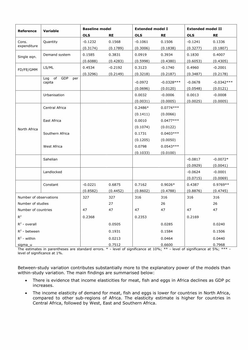
Reference Variable Baseline model Extended model I Extended model II
OLS RE OLS RE OLS RE
Cons. expenditure
Quantity -0.1232 0.1568 -0.1061 0.1506 -0.1241 0.1336
(0.3174) (0.1789) (0.3006) (0.1838) (0.3277) (0.1807)
Single eqn. Demand system 0.1585 0.3831 0.0919 0.3934 0.1830 0.4007
(0.6088) (0.4283) (0.5998) (0.4380) (0.6053) (0.4305)
FD/FE/GMM LS/ML 0.4534 -0.2192 0.3123 -0.1740 0.4960 -0.2001
(0.3296) (0.2149) (0.3218) (0.2187) (0.3487) (0.2178)
Log of GDP per capita -0.0972 -0.0328*** -0.0678 -0.0342***
(0.0696) (0.0120) (0.0548) (0.0121)
Urbanisation 0.0032 -0.0006 0.0013 -0.0008
(0.0031) (0.0005) (0.0025) (0.0005)
North Africa
Central Africa 0.2486* 0.0774***
(0.1411) (0.0066)
East Africa 0.0010 0.0477***
(0.1074) (0.0122)
Southern Africa 0.1731 0.0403***
(0.1205) (0.0050)
West Africa 0.0798 0.0543***
(0.1033) (0.0100)
Sahelian -0.0817 -0.0072*
(0.0929) (0.0041)
Landlocked -0.0624 -0.0001
(0.0715) (0.0069)
Constant -0.0221 0.6875 0.7162 0.9026* 0.4387 0.9769**
(0.8582) (0.4452) (0.8602) (0.4788) (0.8876) (0.4745)
Number of observations 327 327 316 316 316 316
Number of studies 27 26
26
Number of countries 47 47 47 47 47 47
R2 0.2368 0.2353 0.2169
R2 - overall 0.0505 0.0285
0.0240
R2 - between 0.1931 0.1584
0.1506
R2 - within 0.0213 0.0464
0.0440
sigma_u 0.7512 0.6600 0.7968
The estimates in parentheses are standard errors. * - level of significance at 10%; ** - level of significance at 5%; *** - level of significance at 1%.
Between-study variation contributes substantially more to the explanatory power of the models than
within-study variation. The main findings are summarised below:
There is evidence that income elasticities for meat, fish and eggs in Africa declines as GDP pc
increases.
The income elasticity of demand for meat, fish and eggs is lower for countries in North Africa,
compared to other sub-regions of Africa. The elasticity estimate is higher for countries in
Central Africa, followed by West, East and Southern Africa.
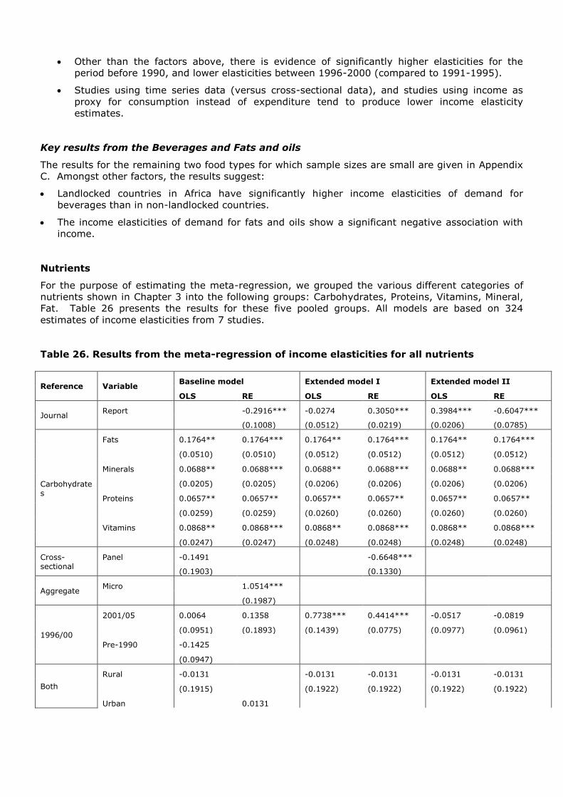
Other than the factors above, there is evidence of significantly higher elasticities for the
period before 1990, and lower elasticities between 1996-2000 (compared to 1991-1995).
Studies using time series data (versus cross-sectional data), and studies using income as
proxy for consumption instead of expenditure tend to produce lower income elasticity
estimates.
Key results from the Beverages and Fats and oils
The results for the remaining two food types for which sample sizes are small are given in Appendix
C. Amongst other factors, the results suggest:
Landlocked countries in Africa have significantly higher income elasticities of demand for
beverages than in non-landlocked countries.
The income elasticities of demand for fats and oils show a significant negative association with
income.
Nutrients
For the purpose of estimating the meta-regression, we grouped the various different categories of
nutrients shown in Chapter 3 into the following groups: Carbohydrates, Proteins, Vitamins, Mineral,
Fat. Table 26 presents the results for these five pooled groups. All models are based on 324
estimates of income elasticities from 7 studies.
Table 26. Results from the meta-regression of income elasticities for all nutrients
Reference Variable Baseline model Extended model I Extended model II
OLS RE OLS RE OLS RE
Journal Report -0.2916*** -0.0274 0.3050*** 0.3984*** -0.6047***
(0.1008) (0.0512) (0.0219) (0.0206) (0.0785)
Carbohydrates
Fats 0.1764** 0.1764*** 0.1764** 0.1764*** 0.1764** 0.1764***
(0.0510) (0.0510) (0.0512) (0.0512) (0.0512) (0.0512)
Minerals 0.0688** 0.0688*** 0.0688** 0.0688*** 0.0688** 0.0688***
(0.0205) (0.0205) (0.0206) (0.0206) (0.0206) (0.0206)
Proteins 0.0657** 0.0657** 0.0657** 0.0657** 0.0657** 0.0657**
(0.0259) (0.0259) (0.0260) (0.0260) (0.0260) (0.0260)
Vitamins 0.0868** 0.0868*** 0.0868** 0.0868*** 0.0868** 0.0868***
(0.0247) (0.0247) (0.0248) (0.0248) (0.0248) (0.0248)
Cross-sectional
Panel -0.1491 -0.6648***
(0.1903) (0.1330)
Aggregate Micro 1.0514***
(0.1987)
1996/00
2001/05 0.0064 0.1358 0.7738*** 0.4414*** -0.0517 -0.0819
(0.0951) (0.1893) (0.1439) (0.0775) (0.0977) (0.0961)
Pre-1990 -0.1425
(0.0947)
Both
Rural -0.0131 -0.0131 -0.0131 -0.0131 -0.0131
(0.1915) (0.1922) (0.1922) (0.1922) (0.1922)
Urban 0.0131
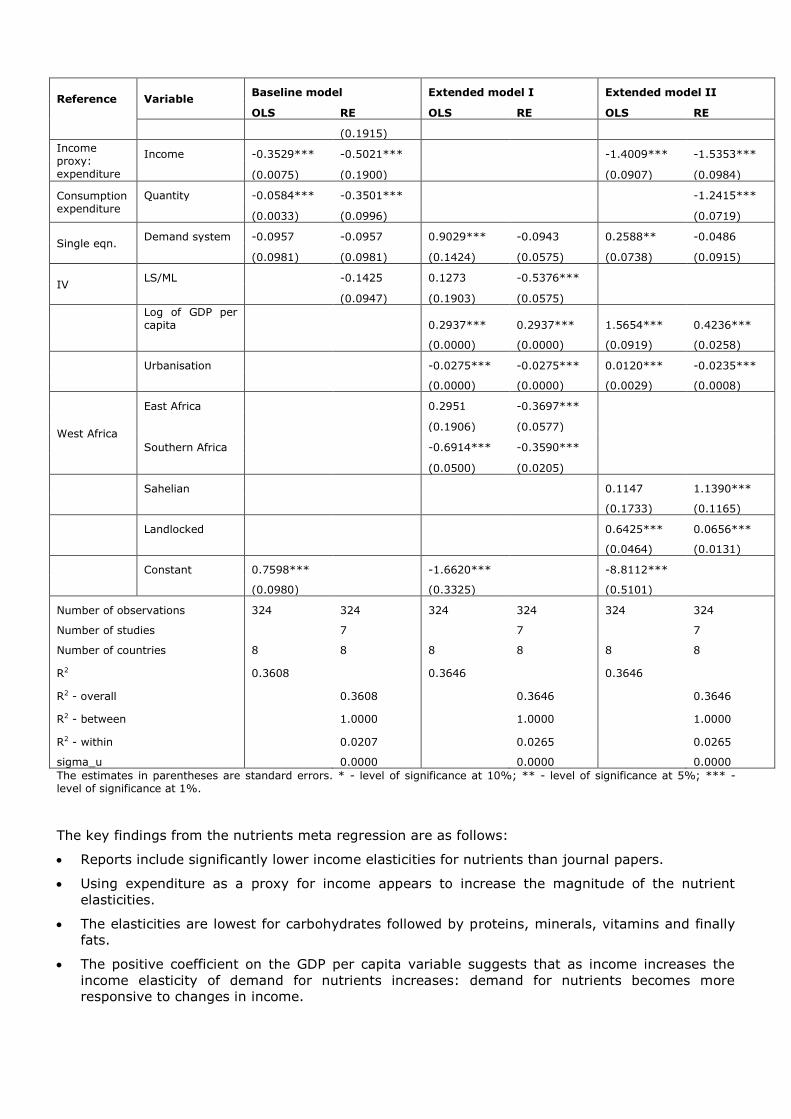
Reference Variable Baseline model Extended model I Extended model II
OLS RE OLS RE OLS RE
(0.1915)
Income proxy: expenditure
Income -0.3529*** -0.5021*** -1.4009*** -1.5353***
(0.0075) (0.1900) (0.0907) (0.0984)
Consumption expenditure
Quantity -0.0584*** -0.3501*** -1.2415***
(0.0033) (0.0996) (0.0719)
Single eqn. Demand system -0.0957 -0.0957 0.9029*** -0.0943 0.2588** -0.0486
(0.0981) (0.0981) (0.1424) (0.0575) (0.0738) (0.0915)
IV LS/ML -0.1425 0.1273 -0.5376***
(0.0947) (0.1903) (0.0575)
Log of GDP per capita 0.2937*** 0.2937*** 1.5654*** 0.4236***
(0.0000) (0.0000) (0.0919) (0.0258)
Urbanisation -0.0275*** -0.0275*** 0.0120*** -0.0235***
(0.0000) (0.0000) (0.0029) (0.0008)
West Africa
East Africa 0.2951 -0.3697***
(0.1906) (0.0577)
Southern Africa -0.6914*** -0.3590***
(0.0500) (0.0205)
Sahelian 0.1147 1.1390***
(0.1733) (0.1165)
Landlocked 0.6425*** 0.0656***
(0.0464) (0.0131)
Constant 0.7598*** -1.6620*** -8.8112***
(0.0980) (0.3325) (0.5101)
Number of observations 324 324 324 324 324 324
Number of studies 7 7 7
Number of countries 8 8 8 8 8 8
R2 0.3608 0.3646 0.3646
R2 - overall 0.3608 0.3646 0.3646
R2 - between 1.0000 1.0000 1.0000
R2 - within 0.0207 0.0265 0.0265
sigma_u 0.0000 0.0000 0.0000
The estimates in parentheses are standard errors. * - level of significance at 10%; ** - level of significance at 5%; *** - level of significance at 1%.
The key findings from the nutrients meta regression are as follows:
Reports include significantly lower income elasticities for nutrients than journal papers.
Using expenditure as a proxy for income appears to increase the magnitude of the nutrient
elasticities.
The elasticities are lowest for carbohydrates followed by proteins, minerals, vitamins and finally
fats.
The positive coefficient on the GDP per capita variable suggests that as income increases the
income elasticity of demand for nutrients increases: demand for nutrients becomes more
responsive to changes in income.
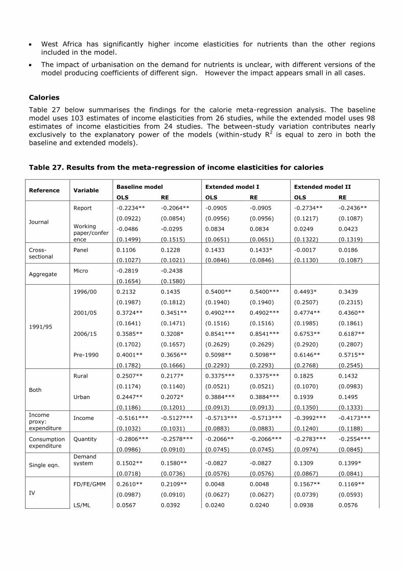
West Africa has significantly higher income elasticities for nutrients than the other regions
included in the model.
The impact of urbanisation on the demand for nutrients is unclear, with different versions of the
model producing coefficients of different sign. However the impact appears small in all cases.
Calories
Table 27 below summarises the findings for the calorie meta-regression analysis. The baseline
model uses 103 estimates of income elasticities from 26 studies, while the extended model uses 98
estimates of income elasticities from 24 studies. The between-study variation contributes nearly
exclusively to the explanatory power of the models (within-study R2 is equal to zero in both the
baseline and extended models).
Table 27. Results from the meta-regression of income elasticities for calories
Reference Variable Baseline model Extended model I Extended model II
OLS RE OLS RE OLS RE
Journal
Report -0.2234** -0.2064** -0.0905 -0.0905 -0.2734** -0.2436**
(0.0922) (0.0854) (0.0956) (0.0956) (0.1217) (0.1087)
Working paper/conference
-0.0486 -0.0295 0.0834 0.0834 0.0249 0.0423
(0.1499) (0.1515) (0.0651) (0.0651) (0.1322) (0.1319)
Cross-sectional
Panel 0.1106 0.1228 0.1433 0.1433* -0.0017 0.0186
(0.1027) (0.1021) (0.0846) (0.0846) (0.1130) (0.1087)
Aggregate Micro -0.2819 -0.2438
(0.1654) (0.1580)
1991/95
1996/00 0.2132 0.1435 0.5400** 0.5400*** 0.4493* 0.3439
(0.1987) (0.1812) (0.1940) (0.1940) (0.2507) (0.2315)
2001/05 0.3724** 0.3451** 0.4902*** 0.4902*** 0.4774** 0.4360**
(0.1641) (0.1471) (0.1516) (0.1516) (0.1985) (0.1861)
2006/15 0.3585** 0.3208* 0.8541*** 0.8541*** 0.6753** 0.6187**
(0.1702) (0.1657) (0.2629) (0.2629) (0.2920) (0.2807)
Pre-1990 0.4001** 0.3656** 0.5098** 0.5098** 0.6146** 0.5715**
(0.1782) (0.1666) (0.2293) (0.2293) (0.2768) (0.2545)
Both
Rural 0.2507** 0.2177* 0.3375*** 0.3375*** 0.1825 0.1432
(0.1174) (0.1140) (0.0521) (0.0521) (0.1070) (0.0983)
Urban 0.2447** 0.2072* 0.3884*** 0.3884*** 0.1939 0.1495
(0.1186) (0.1201) (0.0913) (0.0913) (0.1350) (0.1333)
Income proxy: expenditure
Income -0.5161*** -0.5127*** -0.5713*** -0.5713*** -0.3992*** -0.4173***
(0.1032) (0.1031) (0.0883) (0.0883) (0.1240) (0.1188)
Consumption expenditure
Quantity -0.2806*** -0.2578*** -0.2066** -0.2066*** -0.2783*** -0.2554***
(0.0986) (0.0910) (0.0745) (0.0745) (0.0974) (0.0845)
Single eqn.
Demand system 0.1502** 0.1580** -0.0827 -0.0827 0.1309 0.1399*
(0.0718) (0.0736) (0.0576) (0.0576) (0.0867) (0.0841)
IV
FD/FE/GMM 0.2610** 0.2109** 0.0048 0.0048 0.1567** 0.1169**
(0.0987) (0.0910) (0.0627) (0.0627) (0.0739) (0.0593)
LS/ML 0.0567 0.0392 0.0240 0.0240 0.0938 0.0576
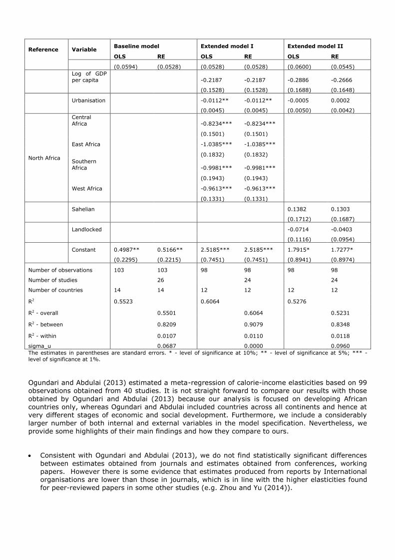
Reference Variable Baseline model Extended model I Extended model II
OLS RE OLS RE OLS RE
(0.0594) (0.0528) (0.0528) (0.0528) (0.0600) (0.0545)
Log of GDP per capita -0.2187 -0.2187 -0.2886 -0.2666
(0.1528) (0.1528) (0.1688) (0.1648)
Urbanisation -0.0112** -0.0112** -0.0005 0.0002
(0.0045) (0.0045) (0.0050) (0.0042)
North Africa
Central Africa -0.8234*** -0.8234***
(0.1501) (0.1501)
East Africa -1.0385*** -1.0385***
(0.1832) (0.1832)
Southern Africa -0.9981*** -0.9981***
(0.1943) (0.1943)
West Africa -0.9613*** -0.9613***
(0.1331) (0.1331)
Sahelian 0.1382 0.1303
(0.1712) (0.1687)
Landlocked -0.0714 -0.0403
(0.1116) (0.0954)
Constant 0.4987** 0.5166** 2.5185*** 2.5185*** 1.7915* 1.7277*
(0.2295) (0.2215) (0.7451) (0.7451) (0.8941) (0.8974)
Number of observations 103 103 98 98 98 98
Number of studies 26 24 24
Number of countries 14 14 12 12 12 12
R2 0.5523 0.6064 0.5276
R2 - overall 0.5501 0.6064 0.5231
R2 - between 0.8209 0.9079 0.8348
R2 - within 0.0107 0.0110 0.0118
sigma_u 0.0687 0.0000 0.0960
The estimates in parentheses are standard errors. * - level of significance at 10%; ** - level of significance at 5%; *** - level of significance at 1%.
Ogundari and Abdulai (2013) estimated a meta-regression of calorie-income elasticities based on 99
observations obtained from 40 studies. It is not straight forward to compare our results with those
obtained by Ogundari and Abdulai (2013) because our analysis is focused on developing African
countries only, whereas Ogundari and Abdulai included countries across all continents and hence at
very different stages of economic and social development. Furthermore, we include a considerably
larger number of both internal and external variables in the model specification. Nevertheless, we
provide some highlights of their main findings and how they compare to ours.
Consistent with Ogundari and Abdulai (2013), we do not find statistically significant differences
between estimates obtained from journals and estimates obtained from conferences, working
papers. However there is some evidence that estimates produced from reports by International
organisations are lower than those in journals, which is in line with the higher elasticities found
for peer-reviewed papers in some other studies (e.g. Zhou and Yu (2014)).
Ogundari and Abdulai find evidence in favour of higher calorie-income elasticities for studies
based on panel data and time series data, compared to cross-sectional data. They also find that
the year of the primary study and the number of years of primary data affect (reduce) the
magnitude of the calorie-income elasticity. However, they do not find any significant effect for
the use of IV type estimators nor the number of regressors used in the primary study.
Compared to their analysis, methodological factors do not appear to play an important role in
explaining the variation across income elasticities in our study. The baseline model suggests that
demand systems produce higher income elasticities than single equation models but this
difference is not evident in the extended versions of the model. Our findins also confirm that
using expenditure as a proxy for income results in higher calorie-income elasticity estimates.
While Ogundari and Abdulai (2013) find evidence of significant differences in the calorie-income
elasticity between Europe, North America and South America (but not between Europe, Africa,
Asia and Oceania): calorie-income elasticities in Europe are found to be higher (lower) than in
North America (South America). Our analysis considers only African countries and suggests that
countries in East and South Africa have lower calorie income elasticities than countries in North
Africa.
Other findings include:
There is evidence that between 1990 and 1995, calorie elasticities fell but then increased in
later periods. It is difficult to reconcile these results to those obtained for all foods and the
more limited sample size might be influencing the robustness of these findings.
There is no effect of GDP per capita on the magnitude of the calorie-income elasticities.
There is evidence that the degree of urbanisation of a country negatively affects the
magnitude of the calorie-income elasticities with calorie income elasticities smaller for more
urbanised economies, all other factors being the same.
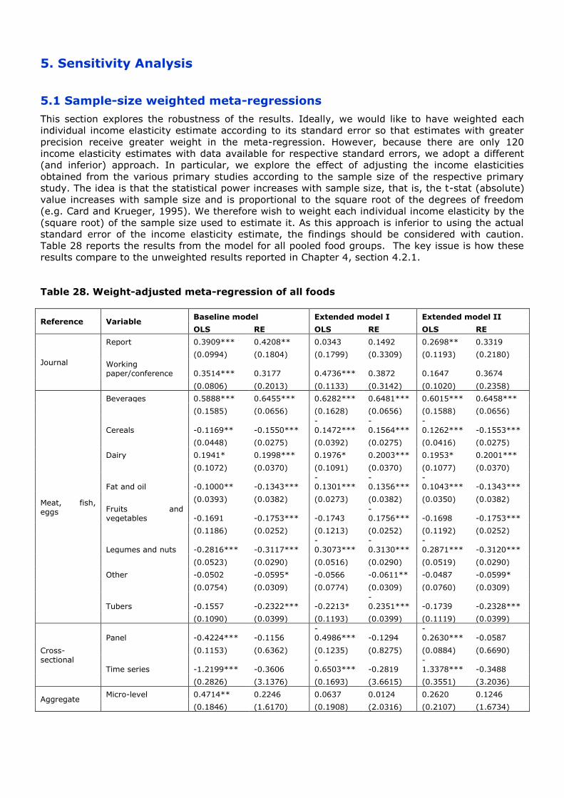
5. Sensitivity Analysis
5.1 Sample-size weighted meta-regressions
This section explores the robustness of the results. Ideally, we would like to have weighted each
individual income elasticity estimate according to its standard error so that estimates with greater
precision receive greater weight in the meta-regression. However, because there are only 120
income elasticity estimates with data available for respective standard errors, we adopt a different
(and inferior) approach. In particular, we explore the effect of adjusting the income elasticities
obtained from the various primary studies according to the sample size of the respective primary
study. The idea is that the statistical power increases with sample size, that is, the t-stat (absolute)
value increases with sample size and is proportional to the square root of the degrees of freedom
(e.g. Card and Krueger, 1995). We therefore wish to weight each individual income elasticity by the
(square root) of the sample size used to estimate it. As this approach is inferior to using the actual
standard error of the income elasticity estimate, the findings should be considered with caution.
Table 28 reports the results from the model for all pooled food groups. The key issue is how these
results compare to the unweighted results reported in Chapter 4, section 4.2.1.
Table 28. Weight-adjusted meta-regression of all foods
Reference Variable Baseline model Extended model I Extended model II
OLS RE OLS RE OLS RE
Journal
Report 0.3909*** 0.4208** 0.0343 0.1492 0.2698** 0.3319
(0.0994) (0.1804) (0.1799) (0.3309) (0.1193) (0.2180)
Working paper/conference 0.3514*** 0.3177 0.4736*** 0.3872 0.1647 0.3674
(0.0806) (0.2013) (0.1133) (0.3142) (0.1020) (0.2358)
Meat, fish, eggs
Beverages 0.5888*** 0.6455*** 0.6282*** 0.6481*** 0.6015*** 0.6458***
(0.1585) (0.0656) (0.1628) (0.0656) (0.1588) (0.0656)
Cereals -0.1169** -0.1550*** -0.1472***
-0.1564***
-0.1262*** -0.1553***
(0.0448) (0.0275) (0.0392) (0.0275) (0.0416) (0.0275)
Dairy 0.1941* 0.1998*** 0.1976* 0.2003*** 0.1953* 0.2001***
(0.1072) (0.0370) (0.1091) (0.0370) (0.1077) (0.0370)
Fat and oil -0.1000** -0.1343*** -0.1301***
-0.1356***
-0.1043*** -0.1343***
(0.0393) (0.0382) (0.0273) (0.0382) (0.0350) (0.0382)
Fruits and vegetables -0.1691 -0.1753*** -0.1743
-0.1756*** -0.1698 -0.1753***
(0.1186) (0.0252) (0.1213) (0.0252) (0.1192) (0.0252)
Legumes and nuts -0.2816*** -0.3117*** -0.3073***
-0.3130***
-0.2871*** -0.3120***
(0.0523) (0.0290) (0.0516) (0.0290) (0.0519) (0.0290)
Other -0.0502 -0.0595* -0.0566 -0.0611** -0.0487 -0.0599*
(0.0754) (0.0309) (0.0774) (0.0309) (0.0760) (0.0309)
Tubers -0.1557 -0.2322*** -0.2213* -0.2351*** -0.1739 -0.2328***
(0.1090) (0.0399) (0.1193) (0.0399) (0.1119) (0.0399)
Cross-sectional
Panel -0.4224*** -0.1156 -0.4986*** -0.1294
-0.2630*** -0.0587
(0.1153) (0.6362) (0.1235) (0.8275) (0.0884) (0.6690)
Time series -1.2199*** -0.3606 -0.6503*** -0.2819
-1.3378*** -0.3488
(0.2826) (3.1376) (0.1693) (3.6615) (0.3551) (3.2036)
Aggregate Micro-level 0.4714** 0.2246 0.0637 0.0124 0.2620 0.1246
(0.1846) (1.6170) (0.1908) (2.0316) (0.2107) (1.6734)
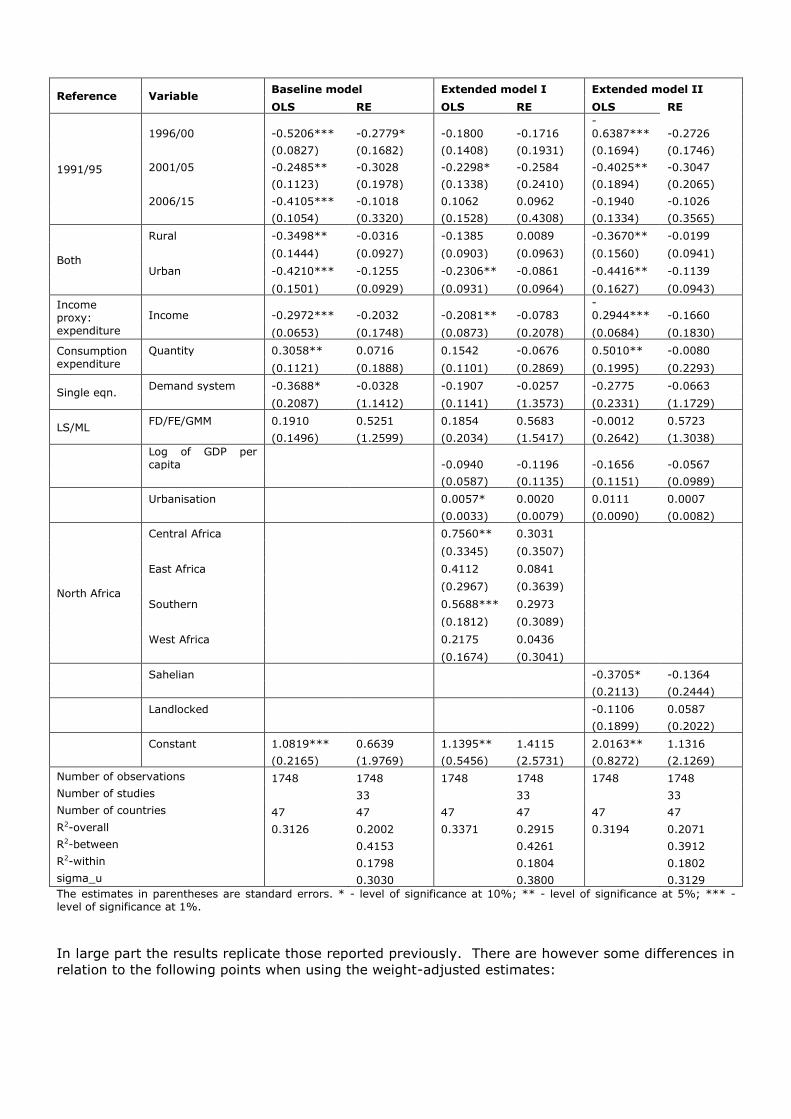
Reference Variable Baseline model Extended model I Extended model II
OLS RE OLS RE OLS RE
1991/95
1996/00 -0.5206*** -0.2779* -0.1800 -0.1716 -0.6387*** -0.2726
(0.0827) (0.1682) (0.1408) (0.1931) (0.1694) (0.1746)
2001/05 -0.2485** -0.3028 -0.2298* -0.2584 -0.4025** -0.3047
(0.1123) (0.1978) (0.1338) (0.2410) (0.1894) (0.2065)
2006/15 -0.4105*** -0.1018 0.1062 0.0962 -0.1940 -0.1026
(0.1054) (0.3320) (0.1528) (0.4308) (0.1334) (0.3565)
Both
Rural -0.3498** -0.0316 -0.1385 0.0089 -0.3670** -0.0199
(0.1444) (0.0927) (0.0903) (0.0963) (0.1560) (0.0941)
Urban -0.4210*** -0.1255 -0.2306** -0.0861 -0.4416** -0.1139
(0.1501) (0.0929) (0.0931) (0.0964) (0.1627) (0.0943)
Income proxy: expenditure
Income -0.2972*** -0.2032 -0.2081** -0.0783 -0.2944*** -0.1660
(0.0653) (0.1748) (0.0873) (0.2078) (0.0684) (0.1830)
Consumption expenditure
Quantity 0.3058** 0.0716 0.1542 -0.0676 0.5010** -0.0080
(0.1121) (0.1888) (0.1101) (0.2869) (0.1995) (0.2293)
Single eqn. Demand system -0.3688* -0.0328 -0.1907 -0.0257 -0.2775 -0.0663
(0.2087) (1.1412) (0.1141) (1.3573) (0.2331) (1.1729)
LS/ML FD/FE/GMM 0.1910 0.5251 0.1854 0.5683 -0.0012 0.5723
(0.1496) (1.2599) (0.2034) (1.5417) (0.2642) (1.3038)
Log of GDP per capita -0.0940 -0.1196 -0.1656 -0.0567
(0.0587) (0.1135) (0.1151) (0.0989)
Urbanisation 0.0057* 0.0020 0.0111 0.0007
(0.0033) (0.0079) (0.0090) (0.0082)
North Africa
Central Africa 0.7560** 0.3031
(0.3345) (0.3507)
East Africa 0.4112 0.0841
(0.2967) (0.3639)
Southern 0.5688*** 0.2973
(0.1812) (0.3089)
West Africa 0.2175 0.0436
(0.1674) (0.3041)
Sahelian -0.3705* -0.1364
(0.2113) (0.2444)
Landlocked -0.1106 0.0587
(0.1899) (0.2022)
Constant 1.0819*** 0.6639 1.1395** 1.4115 2.0163** 1.1316
(0.2165) (1.9769) (0.5456) (2.5731) (0.8272) (2.1269)
Number of observations 1748 1748 1748 1748 1748 1748
Number of studies 33 33 33
Number of countries 47 47 47 47 47 47
R2-overall 0.3126 0.2002 0.3371 0.2915 0.3194 0.2071
R2-between 0.4153 0.4261 0.3912
R2-within 0.1798 0.1804 0.1802
sigma_u 0.3030 0.3800 0.3129
The estimates in parentheses are standard errors. * - level of significance at 10%; ** - level of significance at 5%; *** - level of significance at 1%.
In large part the results replicate those reported previously. There are however some differences in
relation to the following points when using the weight-adjusted estimates:
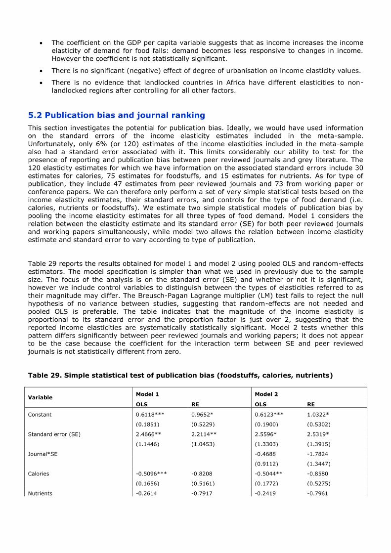
The coefficient on the GDP per capita variable suggests that as income increases the income
elasticity of demand for food falls: demand becomes less responsive to changes in income.
However the coefficient is not statistically significant.
There is no significant (negative) effect of degree of urbanisation on income elasticity values.
There is no evidence that landlocked countries in Africa have different elasticities to non-
landlocked regions after controlling for all other factors.
5.2 Publication bias and journal ranking
This section investigates the potential for publication bias. Ideally, we would have used information
on the standard errors of the income elasticity estimates included in the meta-sample.
Unfortunately, only 6% (or 120) estimates of the income elasticities included in the meta-sample
also had a standard error associated with it. This limits considerably our ability to test for the
presence of reporting and publication bias between peer reviewed journals and grey literature. The
120 elasticity estimates for which we have information on the associated standard errors include 30
estimates for calories, 75 estimates for foodstuffs, and 15 estimates for nutrients. As for type of
publication, they include 47 estimates from peer reviewed journals and 73 from working paper or
conference papers. We can therefore only perform a set of very simple statistical tests based on the
income elasticity estimates, their standard errors, and controls for the type of food demand (i.e.
calories, nutrients or foodstuffs). We estimate two simple statistical models of publication bias by
pooling the income elasticity estimates for all three types of food demand. Model 1 considers the
relation between the elasticity estimate and its standard error (SE) for both peer reviewed journals
and working papers simultaneously, while model two allows the relation between income elasticity
estimate and standard error to vary according to type of publication.
Table 29 reports the results obtained for model 1 and model 2 using pooled OLS and random-effects
estimators. The model specification is simpler than what we used in previously due to the sample
size. The focus of the analysis is on the standard error (SE) and whether or not it is significant,
however we include control variables to distinguish between the types of elasticities referred to as
their magnitude may differ. The Breusch-Pagan Lagrange multiplier (LM) test fails to reject the null
hypothesis of no variance between studies, suggesting that random-effects are not needed and
pooled OLS is preferable. The table indicates that the magnitude of the income elasticity is
proportional to its standard error and the proportion factor is just over 2, suggesting that the
reported income elasticities are systematically statistically significant. Model 2 tests whether this
pattern differs significantly between peer reviewed journals and working papers; it does not appear
to be the case because the coefficient for the interaction term between SE and peer reviewed
journals is not statistically different from zero.
Table 29. Simple statistical test of publication bias (foodstuffs, calories, nutrients)
Variable Model 1 Model 2
OLS RE OLS RE
Constant 0.6118*** 0.9652* 0.6123*** 1.0322*
(0.1851) (0.5229) (0.1900) (0.5302)
Standard error (SE) 2.4666** 2.2114** 2.5596* 2.5319*
(1.1446) (1.0453) (1.3303) (1.3915)
Journal*SE -0.4688 -1.7824
(0.9112) (1.3447)
Calories -0.5096*** -0.8208 -0.5044** -0.8580
(0.1656) (0.5161) (0.1772) (0.5275)
Nutrients -0.2614 -0.7917 -0.2419 -0.7961
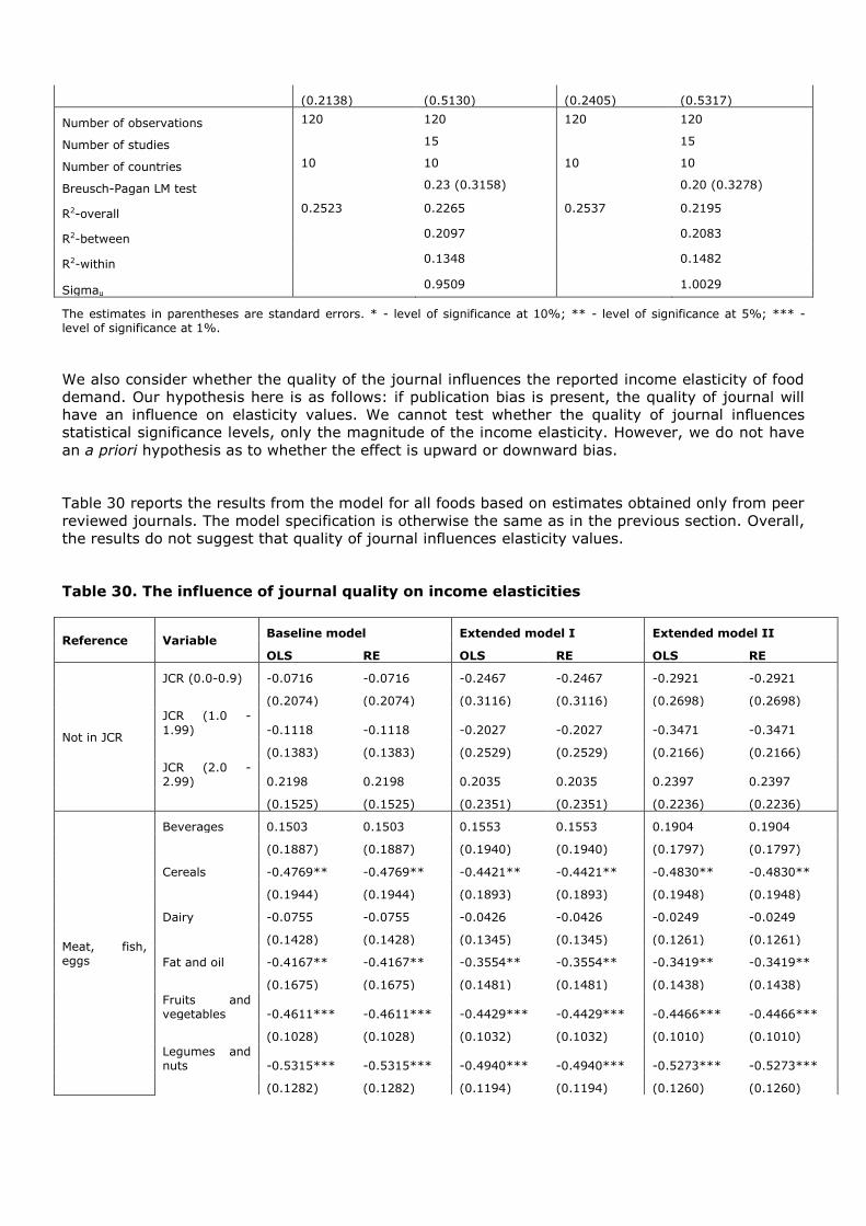
(0.2138) (0.5130) (0.2405) (0.5317)
Number of observations 120 120 120 120
Number of studies 15
15
Number of countries 10 10 10 10
Breusch-Pagan LM test 0.23 (0.3158)
0.20 (0.3278)
R2-overall 0.2523 0.2265 0.2537 0.2195
R2-between 0.2097
0.2083
R2-within 0.1348
0.1482
Sigmau 0.9509 1.0029
The estimates in parentheses are standard errors. * - level of significance at 10%; ** - level of significance at 5%; *** - level of significance at 1%.
We also consider whether the quality of the journal influences the reported income elasticity of food
demand. Our hypothesis here is as follows: if publication bias is present, the quality of journal will
have an influence on elasticity values. We cannot test whether the quality of journal influences
statistical significance levels, only the magnitude of the income elasticity. However, we do not have
an a priori hypothesis as to whether the effect is upward or downward bias.
Table 30 reports the results from the model for all foods based on estimates obtained only from peer
reviewed journals. The model specification is otherwise the same as in the previous section. Overall,
the results do not suggest that quality of journal influences elasticity values.
Table 30. The influence of journal quality on income elasticities
Reference Variable Baseline model Extended model I Extended model II
OLS RE OLS RE OLS RE
Not in JCR
JCR (0.0-0.9) -0.0716 -0.0716 -0.2467 -0.2467 -0.2921 -0.2921
(0.2074) (0.2074) (0.3116) (0.3116) (0.2698) (0.2698)
JCR (1.0 -
1.99) -0.1118 -0.1118 -0.2027 -0.2027 -0.3471 -0.3471
(0.1383) (0.1383) (0.2529) (0.2529) (0.2166) (0.2166)
JCR (2.0 - 2.99) 0.2198 0.2198 0.2035 0.2035 0.2397 0.2397
(0.1525) (0.1525) (0.2351) (0.2351) (0.2236) (0.2236)
Meat, fish, eggs
Beverages 0.1503 0.1503 0.1553 0.1553 0.1904 0.1904
(0.1887) (0.1887) (0.1940) (0.1940) (0.1797) (0.1797)
Cereals -0.4769** -0.4769** -0.4421** -0.4421** -0.4830** -0.4830**
(0.1944) (0.1944) (0.1893) (0.1893) (0.1948) (0.1948)
Dairy -0.0755 -0.0755 -0.0426 -0.0426 -0.0249 -0.0249
(0.1428) (0.1428) (0.1345) (0.1345) (0.1261) (0.1261)
Fat and oil -0.4167** -0.4167** -0.3554** -0.3554** -0.3419** -0.3419**
(0.1675) (0.1675) (0.1481) (0.1481) (0.1438) (0.1438)
Fruits and vegetables -0.4611*** -0.4611*** -0.4429*** -0.4429*** -0.4466*** -0.4466***
(0.1028) (0.1028) (0.1032) (0.1032) (0.1010) (0.1010)
Legumes and nuts -0.5315*** -0.5315*** -0.4940*** -0.4940*** -0.5273*** -0.5273***
(0.1282) (0.1282) (0.1194) (0.1194) (0.1260) (0.1260)
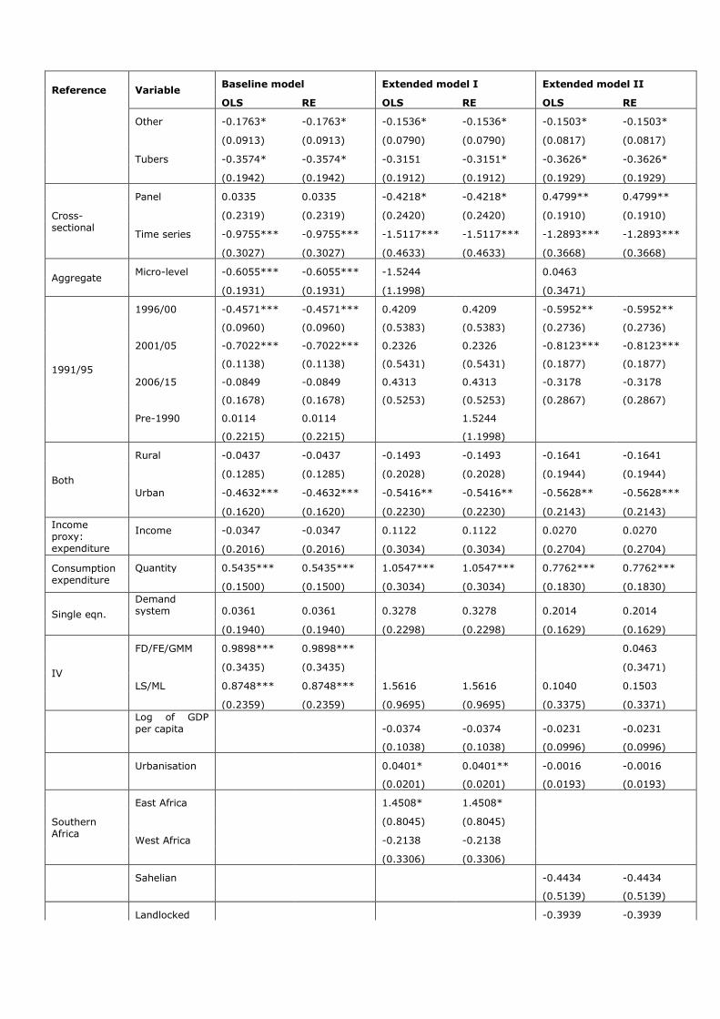
Reference Variable Baseline model Extended model I Extended model II
OLS RE OLS RE OLS RE
Other -0.1763* -0.1763* -0.1536* -0.1536* -0.1503* -0.1503*
(0.0913) (0.0913) (0.0790) (0.0790) (0.0817) (0.0817)
Tubers -0.3574* -0.3574* -0.3151 -0.3151* -0.3626* -0.3626*
(0.1942) (0.1942) (0.1912) (0.1912) (0.1929) (0.1929)
Cross-sectional
Panel 0.0335 0.0335 -0.4218* -0.4218* 0.4799** 0.4799**
(0.2319) (0.2319) (0.2420) (0.2420) (0.1910) (0.1910)
Time series -0.9755*** -0.9755*** -1.5117*** -1.5117*** -1.2893*** -1.2893***
(0.3027) (0.3027) (0.4633) (0.4633) (0.3668) (0.3668)
Aggregate Micro-level -0.6055*** -0.6055*** -1.5244 0.0463
(0.1931) (0.1931) (1.1998) (0.3471)
1991/95
1996/00 -0.4571*** -0.4571*** 0.4209 0.4209 -0.5952** -0.5952**
(0.0960) (0.0960) (0.5383) (0.5383) (0.2736) (0.2736)
2001/05 -0.7022*** -0.7022*** 0.2326 0.2326 -0.8123*** -0.8123***
(0.1138) (0.1138) (0.5431) (0.5431) (0.1877) (0.1877)
2006/15 -0.0849 -0.0849 0.4313 0.4313 -0.3178 -0.3178
(0.1678) (0.1678) (0.5253) (0.5253) (0.2867) (0.2867)
Pre-1990 0.0114 0.0114 1.5244
(0.2215) (0.2215) (1.1998)
Both
Rural -0.0437 -0.0437 -0.1493 -0.1493 -0.1641 -0.1641
(0.1285) (0.1285) (0.2028) (0.2028) (0.1944) (0.1944)
Urban -0.4632*** -0.4632*** -0.5416** -0.5416** -0.5628** -0.5628***
(0.1620) (0.1620) (0.2230) (0.2230) (0.2143) (0.2143)
Income proxy: expenditure
Income -0.0347 -0.0347 0.1122 0.1122 0.0270 0.0270
(0.2016) (0.2016) (0.3034) (0.3034) (0.2704) (0.2704)
Consumption expenditure
Quantity 0.5435*** 0.5435*** 1.0547*** 1.0547*** 0.7762*** 0.7762***
(0.1500) (0.1500) (0.3034) (0.3034) (0.1830) (0.1830)
Single eqn.
Demand system 0.0361 0.0361 0.3278 0.3278 0.2014 0.2014
(0.1940) (0.1940) (0.2298) (0.2298) (0.1629) (0.1629)
IV
FD/FE/GMM 0.9898*** 0.9898*** 0.0463
(0.3435) (0.3435)
(0.3471)
LS/ML 0.8748*** 0.8748*** 1.5616 1.5616 0.1040 0.1503
(0.2359) (0.2359) (0.9695) (0.9695) (0.3375) (0.3371)
Log of GDP per capita -0.0374 -0.0374 -0.0231 -0.0231
(0.1038) (0.1038) (0.0996) (0.0996)
Urbanisation 0.0401* 0.0401** -0.0016 -0.0016
(0.0201) (0.0201) (0.0193) (0.0193)
Southern Africa
East Africa 1.4508* 1.4508*
(0.8045) (0.8045)
West Africa -0.2138 -0.2138
(0.3306) (0.3306)
Sahelian -0.4434 -0.4434
(0.5139) (0.5139)
Landlocked -0.3939 -0.3939
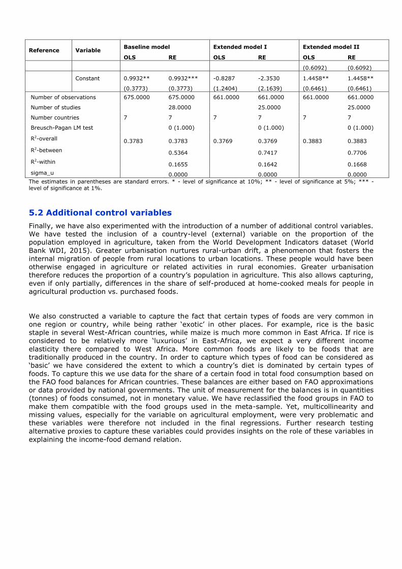
Reference Variable Baseline model Extended model I Extended model II
OLS RE OLS RE OLS RE
(0.6092) (0.6092)
Constant 0.9932** 0.9932*** -0.8287 -2.3530 1.4458** 1.4458**
(0.3773) (0.3773) (1.2404) (2.1639) (0.6461) (0.6461)
Number of observations 675.0000 675.0000 661.0000 661.0000 661.0000 661.0000
Number of studies 28.0000 25.0000 25.0000
Number countries 7 7 7 7 7 7
Breusch-Pagan LM test 0 (1.000) 0 (1.000) 0 (1.000)
R2-overall 0.3783 0.3783 0.3769 0.3769 0.3883 0.3883
R2-between 0.5364 0.7417 0.7706
R2-within 0.1655 0.1642 0.1668
sigma_u 0.0000 0.0000 0.0000
The estimates in parentheses are standard errors. * - level of significance at 10%; ** - level of significance at 5%; *** - level of significance at 1%.
5.2 Additional control variables
Finally, we have also experimented with the introduction of a number of additional control variables.
We have tested the inclusion of a country-level (external) variable on the proportion of the
population employed in agriculture, taken from the World Development Indicators dataset (World
Bank WDI, 2015). Greater urbanisation nurtures rural-urban drift, a phenomenon that fosters the
internal migration of people from rural locations to urban locations. These people would have been
otherwise engaged in agriculture or related activities in rural economies. Greater urbanisation
therefore reduces the proportion of a country’s population in agriculture. This also allows capturing,
even if only partially, differences in the share of self-produced at home-cooked meals for people in
agricultural production vs. purchased foods.
We also constructed a variable to capture the fact that certain types of foods are very common in
one region or country, while being rather ‘exotic’ in other places. For example, rice is the basic
staple in several West-African countries, while maize is much more common in East Africa. If rice is
considered to be relatively more ‘luxurious’ in East-Africa, we expect a very different income
elasticity there compared to West Africa. More common foods are likely to be foods that are
traditionally produced in the country. In order to capture which types of food can be considered as
‘basic’ we have considered the extent to which a country’s diet is dominated by certain types of
foods. To capture this we use data for the share of a certain food in total food consumption based on
the FAO food balances for African countries. These balances are either based on FAO approximations
or data provided by national governments. The unit of measurement for the balances is in quantities
(tonnes) of foods consumed, not in monetary value. We have reclassified the food groups in FAO to
make them compatible with the food groups used in the meta-sample. Yet, multicollinearity and
missing values, especially for the variable on agricultural employment, were very problematic and
these variables were therefore not included in the final regressions. Further research testing
alternative proxies to capture these variables could provides insights on the role of these variables in
explaining the income-food demand relation.

6. Conclusion
The aim of this report was to identify the factors underlying differences in estimates of food income
elasticities within and between developing countries in Africa and, in doing so, to provide greater
understanding of the relationship between income level and the demand of different types of food
and nutrients in the region. This will help in understanding how demand for food, and more
specifically for different types of food and nutrients, can be expected to evolve in the future and
understanding what policies can be used in the fight against malnutrition.
A meta-sample has been constructed including both attributes of the primary studies and external
country-level factors thought to influence the income elasticities. Based on this meta-sample, meta-
regression analyses have been conducted for food-income elasticities (for all foods and separate
types of foods), nutrients, and calorie-income elasticities. The study contributes to previous meta-
analyses of food/calorie demand by focusing entirely on African countries.
A major contribution of the study is associated with the creation of a database of primary studies,
the meta-sample, that can be used (and improved) by other researchers. The meta-sample contains
2,101 elasticity estimates drawn from 66 studies. This study improves upon existing review studies
in a number of ways. First of all, our meta-sample focuses specifically on Africa. Forty-eight out of
54 African countries are represented in the sample. Second, besides demand for calories, we include
elasticity estimates for a whole list of food categories and nutrient types. One of the innovative
features of the study is the inclusion of several “external” variables thought to potentially explain
the heterogeneity across estimated income elasticities. In line with other studies we therefore
include the income level, but we also include the country’s urbanisation rate and three geographical
identifiers. We also control for the potential methodological sources of heterogeneity in estimates.
Unfortunately, it has not been possible to develop comprehensive tests for the presence of
publication bias due to insufficient data for the standard errors of the income elasticities included in
the meta-sample. However, we do explore differences in the income elasticities between studies
according to journal quality.
As expected, the descriptive results indicate that food demand is more responsive to changes in
income (income elasticities are higher) for beverages, meat, fish and eggs and dairy, compared to
foods that tend to constitute basic diets (e.g. cereals, legumes and nuts, fruit and vegetables, and
fats and oils, tubers). Also, the relative magnitude of the different nutrient elasticities was as
expected with higher values for proteins.
Although not all results are fully consistent or significant across the whole set of meta-regressions, a
number of general conclusions can be derived and are in line with our expectations. There is no
strong evidence of major methodological and data-related differences across studies although some
tendencies can be identified. In line with the earlier literature (Bouis and Haddad, 1992), the use of
cross-sectional data tends to result in higher elasticities. The use of household expenditures as a
proxy for income generally results in lower income elasticities, which corresponds to the findings by
Ogundari and Abdulai (2013) and Zhou and Yu (2015) and may relate to the fact that total
expenditure is considered a more reliable proxy than reported income (Deaton, 1997). The use of a
demand system tends to provide higher income elasticities than single equation estimates, which
confirms the findings of Behrman and Deolalikar (1987) and Zhou and Yu (2015).
External factors relating to country income level, time period of primary data, degree of country
urbanisation, and country sub-region have been found to explain heterogeneity in many of the food-
income elasticities. The evolution of the income elasticities with the level of income provides some
interesting results. For calorie demand and food demand in general, we find that in countries with a
higher income level, elasticities are lower. For nutrient demand, we find instead that elasticities are
higher in richer countries. This could potentially indicate that as countries grow richer, households

tend to spend more on food with a more nutritious value. Further analysis would be needed to
investigate this in more detail. Regarding the time period of the study, it is difficult to draw general
conclusions. With respect to the urbanization level, elasticities tend to be lower in urban areas or in
countries with a larger share of urban population. In terms of geographical heterogeneity, elasticities
tend to be consistently higher in North African countries, which is somewhat counter-intuitive given
the higher income level in those countries, after controlling for other expected sources of variability
in the income elasticities. The considerable regional differences in food-income elasticities across
African sub-regions suggests that the impact of food and nutrition policy in Africa is likely to differ by
region. Further research could usefully explore in greater detail some of the patterns identified and,
in doing so, contribute to the design of policies aimed at addressing malnutrition.
7. References
ANDREYEVA, T., LONG, M. W. & BROWNELL, K. D. (2010) The Impact of Food Prices on
Consumption: A Systematic Review of Research on the Price Elasticity of Demand for Food.
American Journal of Public Health, 100(2), 216–222.
ASHENFELTER, O., HARMON, C. & OOSTERBEEK, H. (1999) A Review of Estimates of the
Schooling/Earnings Relationship, with Tests for Publication Bias. Labour Economics, 6(4), 453-470.
BEAUDRY, C. & SCHIFFAUEROVA, A. (2009) Who's Right, Marshall or Jacobs? The Localization
Versus Urbanization Debate. Research Policy, 38, 318-337.
BEHRMAN, J.R. & DEOLALIKAR, A.B. (1987) Will developing country nutrition improve with income?
A case study for rural south India. Journal of Political Economy 95(3): 492-507.
BOUIS, H.E. & HADDAD, L.J. (1992) Are estimates of calorie-income elasticities too high? A
recalibration of the plausible range. Journal of Development Economics, 39(2): 333-364.
CARD, D. & KRUEGER, A. B. (1995) Time-Series Minimum-Wage Studies: A Meta-Analysis. The
American Economic Review, 85(2), 238-243.
CLARK & LINZER (2014) Should I Use Fixed or Random Effects? Political Science Research and
Methods, pp 1 – 10.
DEATON, A. (1997). The Analysis of Household Surveys. A Microeconometric Approach to
Development Policy. Baltimore, MD: Published for the World Bank [by] Johns Hopkins University
Press.
DE GROOT, H. L. F., POOT, J. & SMIT, M. J. (2009) Agglomeration, Innovation and Regional
Development: Theoretical Perspectives and Meta-Analysis. In: CAPELLO, R. & NIJKAMP, P. (eds.)
Handbook of Regional Growth and Development Theories. Cheltenham: Edward Elgar.
DE GROOT, H. L., ABREU, M. & FLORAX, R. J. G. M. (2005) A Meta Analysis of the Effect of Common
Currencies on International Trade. Journal of Economic Surveys, 19, 389-420.
DISDIER, A.-C. & HEAD, K. (2008) The Puzzling Persistence of the Distance Effect on Bilateral Trade.
The Review of Economics and Statistics, 90(1), 37-48.
FAO, IFAD and WFP (2015). The State of Food Insecurity in the World 2015.Meeting the 2015
international hunger targets: taking stock of uneven progress. Rome, FAO.
FABIOSA, J.F. (2011) Globalisation and trends in food consumption. Chapter 23 in The Oxford
Handbook of The Economics of Food Consumption and Politics. Ed Lusk, Roosen and Shorgren.
Oxford Uiversity Press. ISBN 0199681325.
FLORAX, R. J. C. M. (2001) Methodological Pitfalls in Meta-Analysis: Publication Bias. Research
Memorandum 2001-28, Free University Amsterdam.
FLORAX, R. J. C. M. (2002) Accounting for Dependence Among Study Results in Meta-Analysis:
Methodology and Applications to the Valuation and Use of Natural Resources. Research
Memorandum 2002, 5. Free University, Amsterdam.
GREEN, R., CORNELSEN, L., DANGOUR, A. D., TURNER, R., SHANKAR, B., MAZZOCCHI, M. SMITH,
R. D. (2013) The Effect of Rising Food Prices on Food Consumption: Systematic Review with Meta-
Regression. British Medical Journal, 346, 1-9.
GREEN, W.H. (2008) Econometric analysis. 6th ed.Upper Saddle River, N.J.: Prentice Hall
REGMI, A., DEEPAK, M. S., SEALE, J. L. Jr., BERNSTEIN, J. (2001). Cross-Country Analysis of Food
Consumption Patterns. Changing Structure of Global Food Consumption and Trade. Washington,
D.C.: Economic Research Service/USDA.
JENSEN, R. T. & MILLER, N. H. (2011) Do Consumer Price Subsidies Really Improve Nutrition?
Review of Economics and Statistics, 93(4), 1205-1223.
KNELL, M. & STIX, H. (2005) The Income Elasticity of Money Demand: A Meta Analysis of Empirical
Results. Journal of Economic Surveys, 19, 513-533.
LONGHI, S., NIJKAMP, P. & POOT, J. (2005) A Meta Analytic Assessment of the Effect of Immigration
on Wages. Journal of Economic Surveys, 19, 451-477.
MELO, P. C., GRAHAM, D. J. & NOLAND, R. B. (2009) A Meta-Analysis of Estimates of Urban
Agglomeration Economies. Regional Science and Urban Economics, 39, 332-342.
MELO, P.C., GRAHAM, D.J., and BRAGE-ARDAO, R. (2013) The Productivity of Transport
Infrastructure Investment: A Meta-Analysis of Empirical Evidence. Regional Science and Urban
Economics, 43, 695-706.
MUHAMMAD, A., SEALE, J. L. Jr., MEADE, B., and REGMI, A. (2011). International evidence on food
consumption patterns: an update using 2005 International Comparison Program Data, TB-1929, U.
S. Department of Agriculture (USDA), Economic Research Service. March 2011, Revised February
2013, pp. 59.
MURTAUGH, P,A, (2002). Journal quality, effect size, and publication bias in meta-
analysis. Ecology, 83(4), 1162-1166.
NELSON, J. P. & KENNEDY, P. E. (2009) The Use (and Abuse) of Meta-Analysis in Environmental and
Natural Resource Economics: An Assessment, Environmental & Resource Economics, 42 (3), 345-
377.
NIJKAMP, P. & POOT, J. (2005) The Last Word on the Wage Curve? Journal of Economic Surveys,
19, 421-450.
OGUNDARI, K. & ABDULAI, A. (2013) Examining the Heterogeneity in Calorie–Income Elasticities: A
Meta-Analysis. Food Policy, 40, 119-128.
POPKIN, B.M. (1994). The nutrition transition in low-income countries: an emerging crisis. Nutrition
Reviews, 52(9): 285-298.
ROSE, A. K. & STANLEY, T. D. (2005) A Meta Analysis of the Effect of Common Currencies on
International Trade. Journal of Economic Surveys, 19, 347-365.
SALOIS, M. J., TIFFIN, R. & BALCOMBE, K.G. (2012) Impact of Income on Nutrient Intakes:
Implications for Undernourishment and Obesity. Journal of Development Studies, 48(12), 1716-
1730.
SKOUFIAS, E., DI MARO, V., GONZÁLEZ-COSSÍO, T., RAMIREZ, S. R. (2011) Food Quality, Calories
and Household Income. Applied Economics, 42(28), 4331-4342.
STANLEY, T. D. (2001) Wheat from Chaff: Meta-Analysis as Quantitative Literature Review. The
Journal of Economic Perspectives, 15, 131-150.
STANLEY, T. D. (2005) Beyond Publication Bias. Journal of Economic Surveys, 19, 309-345.
STANLEY, T. D. & JARRELL, S. B. (2005) Meta Regression Analysis: A Quantitative Method of
Literature Surveys. Journal of Economic Surveys, 19, 299-308.
STRAUSS, J. & THOMAS, D. (1990) The shape of the calorie-expenditure curve, Center Discussion
Paper No. 595, Economic Growth Center, Yale University.
UNPD - United Nations, Department of Economic and Social Affaires, Population Division (2015).
World Population Prospects: The 2015 Revision, Key Findings and Advance Tables. Working Paper
No., ESA/P/WP/241
WEICHSELBAUMER, D. & WINTER-EBMER, R. (2005) A Meta Analysis of the International Gender
Wage Gap. Journal of Economic Surveys, 19, 479-511.
WORLD BANK (2015) Global Economic Prospects, June 2015: The Global Economy in Transition,
Chapter 2: Sub-Saharan Africa, Washington, DC. World Bank.
WoS JCR (2014). Web of Science - Journal Citation Report 2014. http://admin-
apps.webofknowledge.com/JCR/static_html/notices/notices.htm
ZHOU, D. & YU, X. (2014) Calorie Elasticities with Income Dynamics: Evidence from the Literature.
Global Food Discussion papers, No. 35.
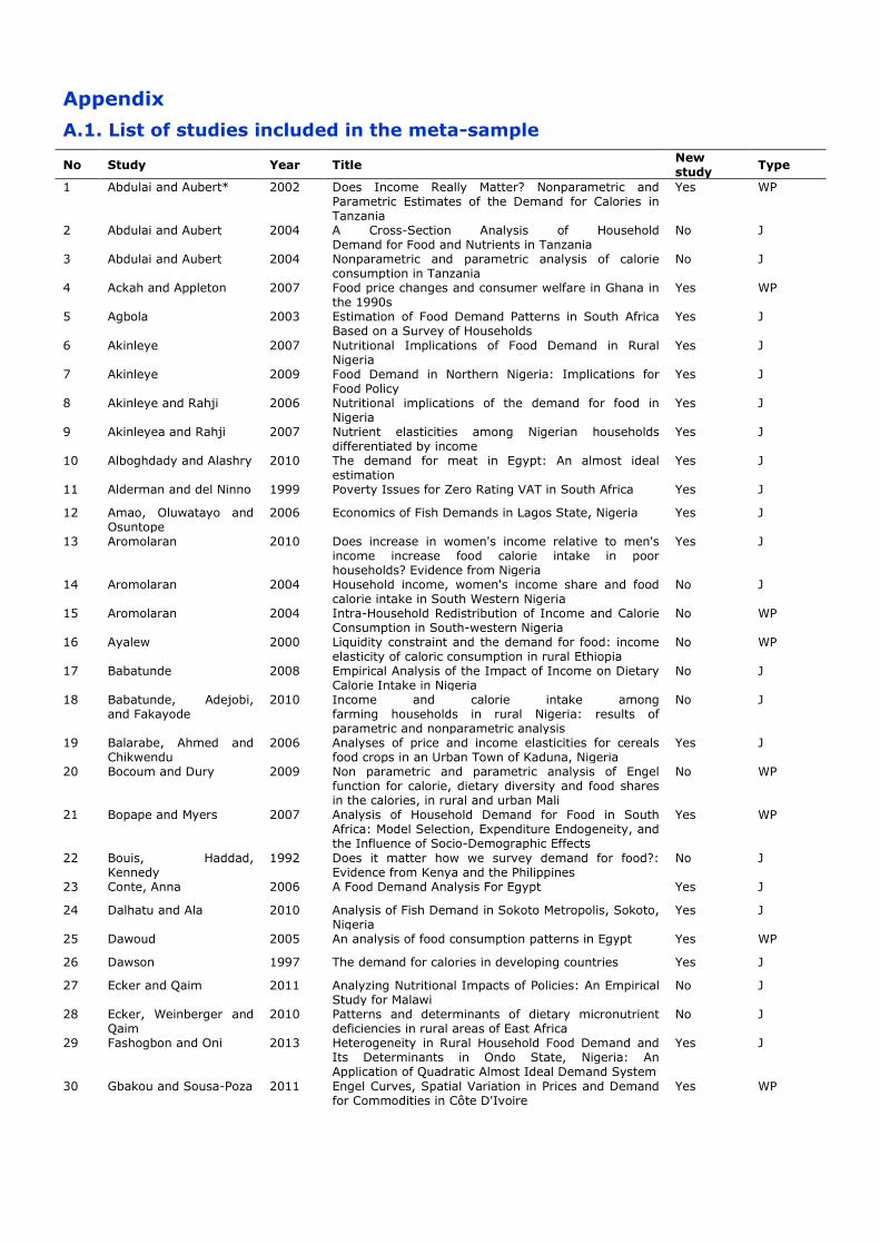
Appendix
A.1. List of studies included in the meta-sample
No Study Year Title New study
Type
1 Abdulai and Aubert* 2002 Does Income Really Matter? Nonparametric and Parametric Estimates of the Demand for Calories in Tanzania
Yes WP
2 Abdulai and Aubert 2004 A Cross-Section Analysis of Household Demand for Food and Nutrients in Tanzania
No J
3 Abdulai and Aubert 2004 Nonparametric and parametric analysis of calorie consumption in Tanzania
No J
4 Ackah and Appleton 2007 Food price changes and consumer welfare in Ghana in the 1990s
Yes WP
5 Agbola 2003 Estimation of Food Demand Patterns in South Africa Based on a Survey of Households
Yes J
6 Akinleye 2007 Nutritional Implications of Food Demand in Rural Nigeria
Yes J
7 Akinleye 2009 Food Demand in Northern Nigeria: Implications for Food Policy
Yes J
8 Akinleye and Rahji 2006 Nutritional implications of the demand for food in Nigeria
Yes J
9 Akinleyea and Rahji 2007 Nutrient elasticities among Nigerian households differentiated by income
Yes J
10 Alboghdady and Alashry 2010 The demand for meat in Egypt: An almost ideal estimation
Yes J
11 Alderman and del Ninno 1999 Poverty Issues for Zero Rating VAT in South Africa Yes J
12 Amao, Oluwatayo and Osuntope
2006 Economics of Fish Demands in Lagos State, Nigeria Yes J
13 Aromolaran 2010 Does increase in women's income relative to men's income increase food calorie intake in poor households? Evidence from Nigeria
Yes J
14 Aromolaran 2004 Household income, women's income share and food calorie intake in South Western Nigeria
No J
15 Aromolaran 2004 Intra-Household Redistribution of Income and Calorie Consumption in South-western Nigeria
No WP
16 Ayalew 2000 Liquidity constraint and the demand for food: income elasticity of caloric consumption in rural Ethiopia
No WP
17 Babatunde 2008 Empirical Analysis of the Impact of Income on Dietary Calorie Intake in Nigeria
No J
18 Babatunde, Adejobi, and Fakayode
2010 Income and calorie intake among farming households in rural Nigeria: results of parametric and nonparametric analysis
No J
19 Balarabe, Ahmed and Chikwendu
2006 Analyses of price and income elasticities for cereals food crops in an Urban Town of Kaduna, Nigeria
Yes J
20 Bocoum and Dury 2009 Non parametric and parametric analysis of Engel function for calorie, dietary diversity and food shares in the calories, in rural and urban Mali
No WP
21 Bopape and Myers 2007 Analysis of Household Demand for Food in South Africa: Model Selection, Expenditure Endogeneity, and the Influence of Socio-Demographic Effects
Yes WP
22 Bouis, Haddad, Kennedy
1992 Does it matter how we survey demand for food?: Evidence from Kenya and the Philippines
No J
23 Conte, Anna 2006 A Food Demand Analysis For Egypt Yes J
24 Dalhatu and Ala 2010 Analysis of Fish Demand in Sokoto Metropolis, Sokoto, Nigeria
Yes J
25 Dawoud 2005 An analysis of food consumption patterns in Egypt Yes WP
26 Dawson 1997 The demand for calories in developing countries Yes J
27 Ecker and Qaim 2011 Analyzing Nutritional Impacts of Policies: An Empirical Study for Malawi
No J
28 Ecker, Weinberger and Qaim
2010 Patterns and determinants of dietary micronutrient deficiencies in rural areas of East Africa
No J
29 Fashogbon and Oni 2013 Heterogeneity in Rural Household Food Demand and Its Determinants in Ondo State, Nigeria: An Application of Quadratic Almost Ideal Demand System
Yes J
30 Gbakou and Sousa-Poza 2011 Engel Curves, Spatial Variation in Prices and Demand for Commodities in Côte D'Ivoire
Yes WP
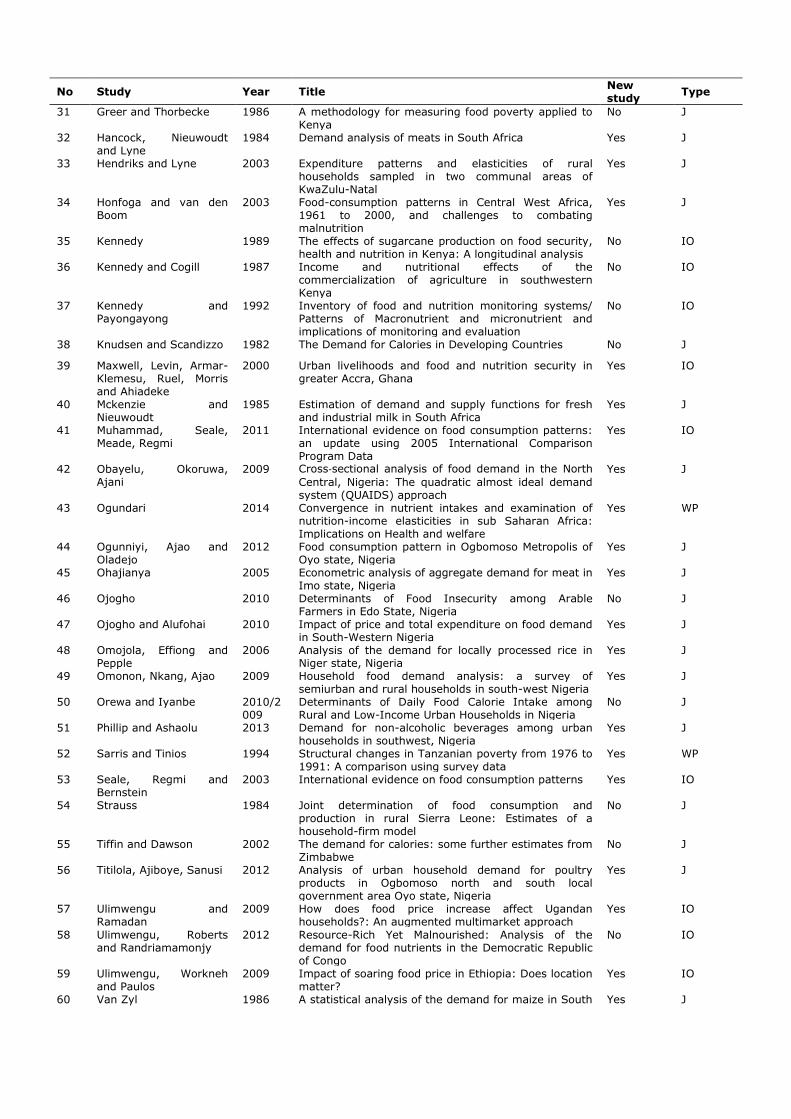
No Study Year Title New study
Type
31 Greer and Thorbecke 1986 A methodology for measuring food poverty applied to Kenya
No J
32 Hancock, Nieuwoudt and Lyne
1984 Demand analysis of meats in South Africa Yes J
33 Hendriks and Lyne 2003 Expenditure patterns and elasticities of rural households sampled in two communal areas of KwaZulu-Natal
Yes J
34 Honfoga and van den Boom
2003 Food-consumption patterns in Central West Africa, 1961 to 2000, and challenges to combating malnutrition
Yes J
35 Kennedy 1989 The effects of sugarcane production on food security, health and nutrition in Kenya: A longitudinal analysis
No IO
36 Kennedy and Cogill 1987 Income and nutritional effects of the commercialization of agriculture in southwestern Kenya
No IO
37 Kennedy and Payongayong
1992 Inventory of food and nutrition monitoring systems/ Patterns of Macronutrient and micronutrient and implications of monitoring and evaluation
No IO
38 Knudsen and Scandizzo 1982 The Demand for Calories in Developing Countries No J
39 Maxwell, Levin, Armar-Klemesu, Ruel, Morris and Ahiadeke
2000 Urban livelihoods and food and nutrition security in greater Accra, Ghana
Yes IO
40 Mckenzie and Nieuwoudt
1985 Estimation of demand and supply functions for fresh and industrial milk in South Africa
Yes J
41 Muhammad, Seale, Meade, Regmi
2011 International evidence on food consumption patterns: an update using 2005 International Comparison Program Data
Yes IO
42 Obayelu, Okoruwa, Ajani
2009 Cross‐sectional analysis of food demand in the North
Central, Nigeria: The quadratic almost ideal demand system (QUAIDS) approach
Yes J
43 Ogundari 2014 Convergence in nutrient intakes and examination of nutrition-income elasticities in sub Saharan Africa: Implications on Health and welfare
Yes WP
44 Ogunniyi, Ajao and Oladejo
2012 Food consumption pattern in Ogbomoso Metropolis of Oyo state, Nigeria
Yes J
45 Ohajianya 2005 Econometric analysis of aggregate demand for meat in Imo state, Nigeria
Yes J
46 Ojogho 2010 Determinants of Food Insecurity among Arable Farmers in Edo State, Nigeria
No J
47 Ojogho and Alufohai 2010 Impact of price and total expenditure on food demand in South-Western Nigeria
Yes J
48 Omojola, Effiong and Pepple
2006 Analysis of the demand for locally processed rice in Niger state, Nigeria
Yes J
49 Omonon, Nkang, Ajao 2009 Household food demand analysis: a survey of semiurban and rural households in south-west Nigeria
Yes J
50 Orewa and Iyanbe 2010/2009
Determinants of Daily Food Calorie Intake among Rural and Low-Income Urban Households in Nigeria
No J
51 Phillip and Ashaolu 2013 Demand for non-alcoholic beverages among urban households in southwest, Nigeria
Yes J
52 Sarris and Tinios 1994 Structural changes in Tanzanian poverty from 1976 to 1991: A comparison using survey data
Yes WP
53 Seale, Regmi and Bernstein
2003 International evidence on food consumption patterns Yes IO
54 Strauss 1984 Joint determination of food consumption and production in rural Sierra Leone: Estimates of a household-firm model
No J
55 Tiffin and Dawson 2002 The demand for calories: some further estimates from Zimbabwe
No J
56 Titilola, Ajiboye, Sanusi 2012 Analysis of urban household demand for poultry products in Ogbomoso north and south local government area Oyo state, Nigeria
Yes J
57 Ulimwengu and Ramadan
2009 How does food price increase affect Ugandan households?: An augmented multimarket approach
Yes IO
58 Ulimwengu, Roberts and Randriamamonjy
2012 Resource-Rich Yet Malnourished: Analysis of the demand for food nutrients in the Democratic Republic of Congo
No IO
59 Ulimwengu, Workneh and Paulos
2009 Impact of soaring food price in Ethiopia: Does location matter?
Yes IO
60 Van Zyl 1986 A statistical analysis of the demand for maize in South Yes J

No Study Year Title New study
Type
Africa
61 von Bach and van Zyl 1994 Human carbohydrate demand in South Africa Yes J
62 von Braun, de Haen, and Blanken
1991 Commercialization of agriculture under population pressure: Effects on production, consumption, and nutrition in Rwanda
No IO
63 von Braun, Puetz, and Webb
1989 Irrigation technology and commercialization of rice in the Gambia: Effects on income and nutririon
No IO
64 Weliwita, Nyange, and Tsujii
2003 Food demand patterns in Tanzania: A censored Regression Analysis of Microdata
Yes J
65 Yusuf 2012 A System Analysis of the Demand for Animal Protein in Rural and Urban Nigeria: A Case Study of Ibadan Metropolis
Yes J
66 Camara 2013 Seasonal price variability and the effective demand for nutrients: Evidence from cereals markets in Mali
Yes J
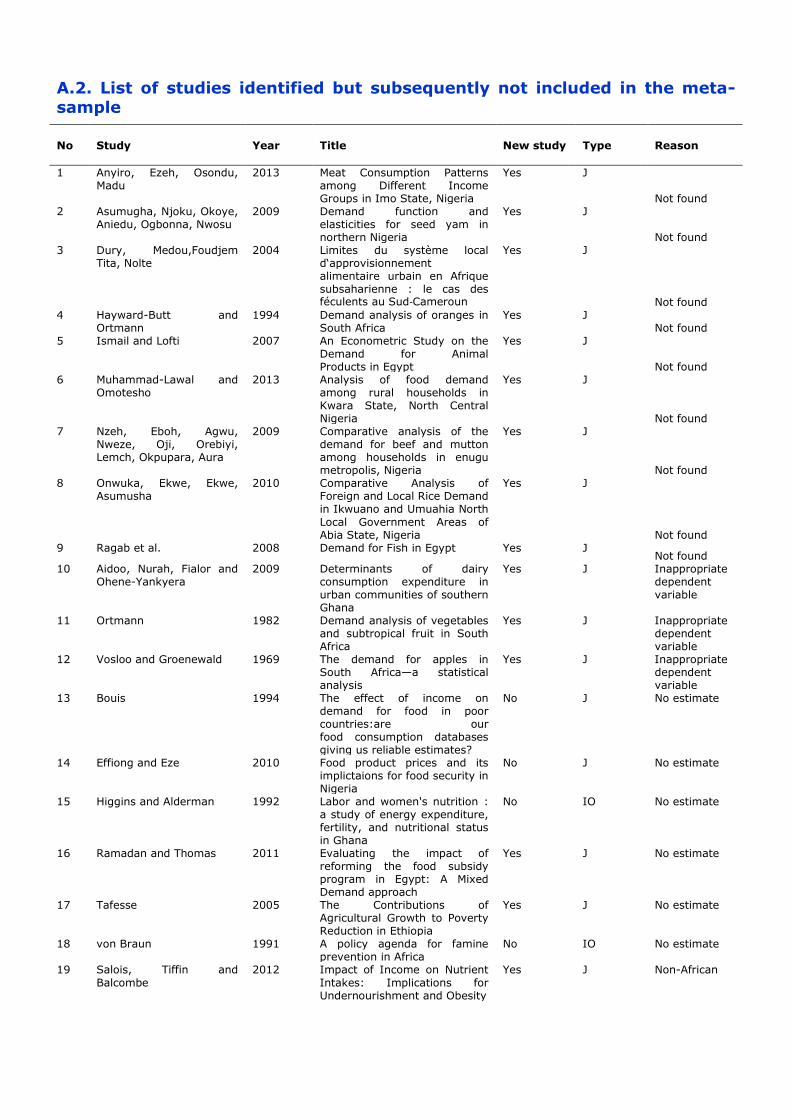
A.2. List of studies identified but subsequently not included in the meta-sample
No Study Year Title New study Type Reason
1 Anyiro, Ezeh, Osondu, Madu
2013 Meat Consumption Patterns among Different Income Groups in Imo State, Nigeria
Yes J
Not found 2 Asumugha, Njoku, Okoye,
Aniedu, Ogbonna, Nwosu 2009 Demand function and
elasticities for seed yam in northern Nigeria
Yes J
Not found 3 Dury, Medou,Foudjem
Tita, Nolte 2004 Limites du système local
d‘approvisionnement alimentaire urbain en Afrique subsaharienne : le cas des féculents au Sud‐Cameroun
Yes J
Not found 4 Hayward-Butt and
Ortmann 1994 Demand analysis of oranges in
South Africa Yes J
Not found 5 Ismail and Lofti 2007 An Econometric Study on the
Demand for Animal Products in Egypt
Yes J
Not found 6 Muhammad-Lawal and
Omotesho 2013 Analysis of food demand
among rural households in Kwara State, North Central Nigeria
Yes J
Not found 7 Nzeh, Eboh, Agwu,
Nweze, Oji, Orebiyi, Lemch, Okpupara, Aura
2009 Comparative analysis of the demand for beef and mutton among households in enugu metropolis, Nigeria
Yes J
Not found 8 Onwuka, Ekwe, Ekwe,
Asumusha 2010 Comparative Analysis of
Foreign and Local Rice Demand in Ikwuano and Umuahia North
Local Government Areas of Abia State, Nigeria
Yes J
Not found 9 Ragab et al. 2008 Demand for Fish in Egypt Yes J
Not found 10 Aidoo, Nurah, Fialor and
Ohene-Yankyera 2009 Determinants of dairy
consumption expenditure in urban communities of southern Ghana
Yes J Inappropriate dependent variable
11 Ortmann 1982 Demand analysis of vegetables and subtropical fruit in South Africa
Yes J Inappropriate dependent variable
12 Vosloo and Groenewald 1969 The demand for apples in South Africa—a statistical analysis
Yes J Inappropriate dependent variable
13 Bouis 1994 The effect of income on demand for food in poor countries:are our food consumption databases giving us reliable estimates?
No J No estimate
14 Effiong and Eze 2010 Food product prices and its implictaions for food security in Nigeria
No J No estimate
15 Higgins and Alderman 1992 Labor and women's nutrition : a study of energy expenditure, fertility, and nutritional status in Ghana
No IO No estimate
16 Ramadan and Thomas 2011 Evaluating the impact of reforming the food subsidy program in Egypt: A Mixed Demand approach
Yes J No estimate
17 Tafesse 2005 The Contributions of Agricultural Growth to Poverty Reduction in Ethiopia
Yes J No estimate
18 von Braun 1991 A policy agenda for famine prevention in Africa
No IO No estimate
19 Salois, Tiffin and
Balcombe
2012 Impact of Income on Nutrient
Intakes: Implications for Undernourishment and Obesity
Yes J Non-African

No Study Year Title New study Type Reason
20 Babatunde 2008 Income Inequality in Rural Nigeria: Evidence from Farming Households Survey Data
Yes J Different subject matter
21 Ojo, Salami and Mohammed
2008 Profitability, inputs elasticities and resource-use efficiency in small scale cowpea production in Niger state, Nigeria
Yes J Different subject matter
22 Onoja and Unaeze 2008 Socio-economic determinants of productivity and income of rice farmers in Udenu local government areas, Enugu state, Nigeria
Yes J Different subject matter
23 Tsue, Lawal, Ayuba 2012 Profit efficiency among catfish farmers in Benue state, Nigeria
Yes J Different subject matter
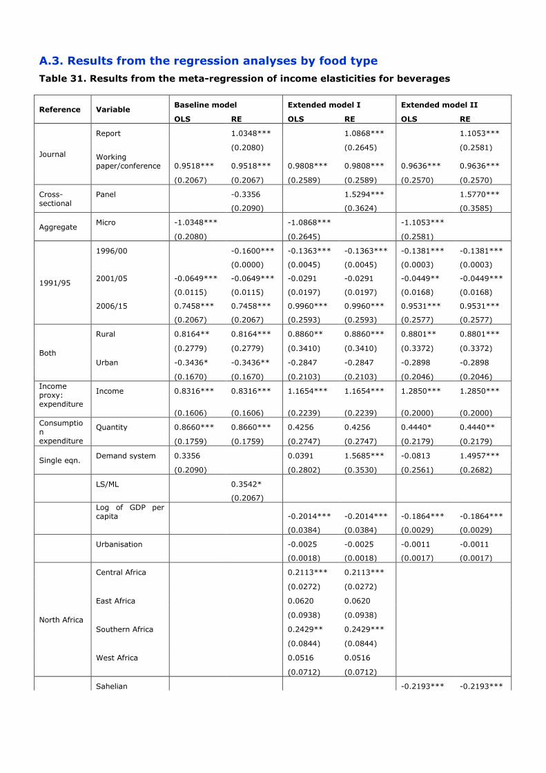
A.3. Results from the regression analyses by food type
Table 31. Results from the meta-regression of income elasticities for beverages
Reference Variable Baseline model Extended model I Extended model II
OLS RE OLS RE OLS RE
Journal
Report 1.0348*** 1.0868*** 1.1053***
(0.2080) (0.2645)
(0.2581)
Working paper/conference 0.9518*** 0.9518*** 0.9808*** 0.9808*** 0.9636*** 0.9636***
(0.2067) (0.2067) (0.2589) (0.2589) (0.2570) (0.2570)
Cross-sectional
Panel -0.3356 1.5294*** 1.5770***
(0.2090) (0.3624)
(0.3585)
Aggregate Micro -1.0348*** -1.0868*** -1.1053***
(0.2080) (0.2645) (0.2581)
1991/95
1996/00 -0.1600*** -0.1363*** -0.1363*** -0.1381*** -0.1381***
(0.0000) (0.0045) (0.0045) (0.0003) (0.0003)
2001/05 -0.0649*** -0.0649*** -0.0291 -0.0291 -0.0449** -0.0449***
(0.0115) (0.0115) (0.0197) (0.0197) (0.0168) (0.0168)
2006/15 0.7458*** 0.7458*** 0.9960*** 0.9960*** 0.9531*** 0.9531***
(0.2067) (0.2067) (0.2593) (0.2593) (0.2577) (0.2577)
Both
Rural 0.8164** 0.8164*** 0.8860** 0.8860*** 0.8801** 0.8801***
(0.2779) (0.2779) (0.3410) (0.3410) (0.3372) (0.3372)
Urban -0.3436* -0.3436** -0.2847 -0.2847 -0.2898 -0.2898
(0.1670) (0.1670) (0.2103) (0.2103) (0.2046) (0.2046)
Income proxy: expenditure
Income 0.8316*** 0.8316*** 1.1654*** 1.1654*** 1.2850*** 1.2850***
(0.1606) (0.1606) (0.2239) (0.2239) (0.2000) (0.2000)
Consumption expenditure
Quantity 0.8660*** 0.8660*** 0.4256 0.4256 0.4440* 0.4440**
(0.1759) (0.1759) (0.2747) (0.2747) (0.2179) (0.2179)
Single eqn. Demand system 0.3356 0.0391 1.5685*** -0.0813 1.4957***
(0.2090) (0.2802) (0.3530) (0.2561) (0.2682)
LS/ML 0.3542*
(0.2067)
Log of GDP per capita -0.2014*** -0.2014*** -0.1864*** -0.1864***
(0.0384) (0.0384) (0.0029) (0.0029)
Urbanisation -0.0025 -0.0025 -0.0011 -0.0011
(0.0018) (0.0018) (0.0017) (0.0017)
North Africa
Central Africa 0.2113*** 0.2113***
(0.0272) (0.0272)
East Africa 0.0620 0.0620
(0.0938) (0.0938)
Southern Africa 0.2429** 0.2429***
(0.0844) (0.0844)
West Africa 0.0516 0.0516
(0.0712) (0.0712)
Sahelian -0.2193*** -0.2193***
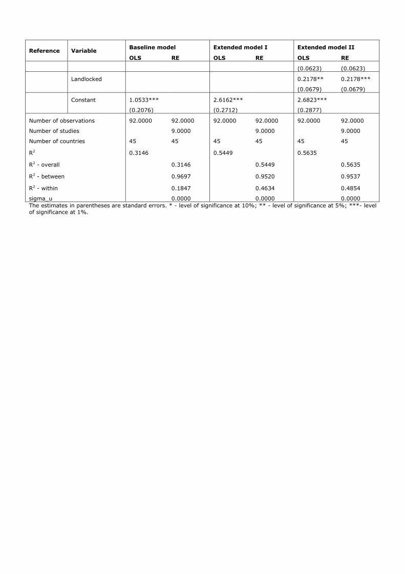
Reference Variable Baseline model Extended model I Extended model II
OLS RE OLS RE OLS RE
(0.0623) (0.0623)
Landlocked 0.2178** 0.2178***
(0.0679) (0.0679)
Constant 1.0533*** 2.6162*** 2.6823***
(0.2076) (0.2712) (0.2877)
Number of observations 92.0000 92.0000 92.0000 92.0000 92.0000 92.0000
Number of studies 9.0000 9.0000
9.0000
Number of countries 45 45 45 45 45 45
R2 0.3146 0.5449 0.5635
R2 - overall 0.3146 0.5449
0.5635
R2 - between 0.9697 0.9520
0.9537
R2 - within 0.1847 0.4634
0.4854
sigma_u 0.0000 0.0000 0.0000
The estimates in parentheses are standard errors. * - level of significance at 10%; ** - level of significance at 5%; ***- level of significance at 1%.
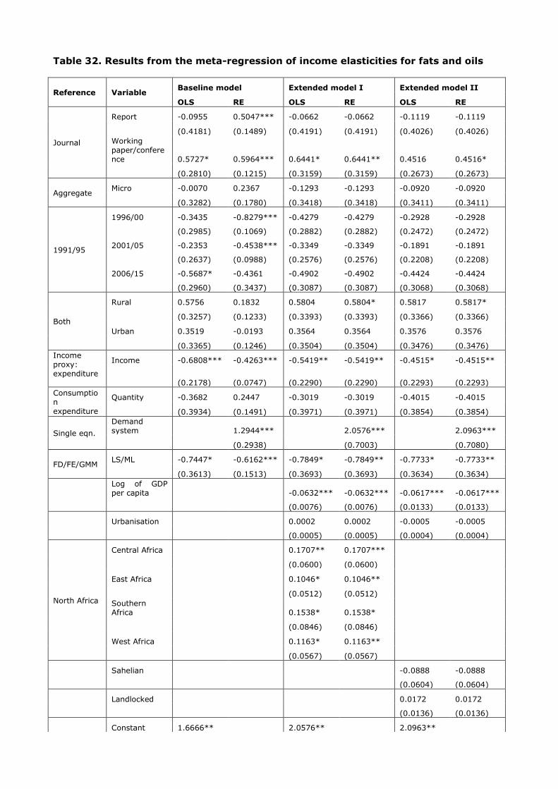
Table 32. Results from the meta-regression of income elasticities for fats and oils
Reference Variable Baseline model Extended model I Extended model II
OLS RE OLS RE OLS RE
Journal
Report -0.0955 0.5047*** -0.0662 -0.0662 -0.1119 -0.1119
(0.4181) (0.1489) (0.4191) (0.4191) (0.4026) (0.4026)
Working paper/conference 0.5727* 0.5964*** 0.6441* 0.6441** 0.4516 0.4516*
(0.2810) (0.1215) (0.3159) (0.3159) (0.2673) (0.2673)
Aggregate Micro -0.0070 0.2367 -0.1293 -0.1293 -0.0920 -0.0920
(0.3282) (0.1780) (0.3418) (0.3418) (0.3411) (0.3411)
1991/95
1996/00 -0.3435 -0.8279*** -0.4279 -0.4279 -0.2928 -0.2928
(0.2985) (0.1069) (0.2882) (0.2882) (0.2472) (0.2472)
2001/05 -0.2353 -0.4538*** -0.3349 -0.3349 -0.1891 -0.1891
(0.2637) (0.0988) (0.2576) (0.2576) (0.2208) (0.2208)
2006/15 -0.5687* -0.4361 -0.4902 -0.4902 -0.4424 -0.4424
(0.2960) (0.3437) (0.3087) (0.3087) (0.3068) (0.3068)
Both
Rural 0.5756 0.1832 0.5804 0.5804* 0.5817 0.5817*
(0.3257) (0.1233) (0.3393) (0.3393) (0.3366) (0.3366)
Urban 0.3519 -0.0193 0.3564 0.3564 0.3576 0.3576
(0.3365) (0.1246) (0.3504) (0.3504) (0.3476) (0.3476)
Income proxy: expenditure
Income -0.6808*** -0.4263*** -0.5419** -0.5419** -0.4515* -0.4515**
(0.2178) (0.0747) (0.2290) (0.2290) (0.2293) (0.2293)
Consumption expenditure
Quantity -0.3682 0.2447 -0.3019 -0.3019 -0.4015 -0.4015
(0.3934) (0.1491) (0.3971) (0.3971) (0.3854) (0.3854)
Single eqn.
Demand system 1.2944*** 2.0576*** 2.0963***
(0.2938) (0.7003) (0.7080)
FD/FE/GMM LS/ML -0.7447* -0.6162*** -0.7849* -0.7849** -0.7733* -0.7733**
(0.3613) (0.1513) (0.3693) (0.3693) (0.3634) (0.3634)
Log of GDP per capita -0.0632*** -0.0632*** -0.0617*** -0.0617***
(0.0076) (0.0076) (0.0133) (0.0133)
Urbanisation 0.0002 0.0002 -0.0005 -0.0005
(0.0005) (0.0005) (0.0004) (0.0004)
North Africa
Central Africa 0.1707** 0.1707***
(0.0600) (0.0600)
East Africa 0.1046* 0.1046**
(0.0512) (0.0512)
Southern Africa 0.1538* 0.1538*
(0.0846) (0.0846)
West Africa 0.1163* 0.1163**
(0.0567) (0.0567)
Sahelian -0.0888 -0.0888
(0.0604) (0.0604)
Landlocked 0.0172 0.0172
(0.0136) (0.0136)
Constant 1.6666** 2.0576** 2.0963**
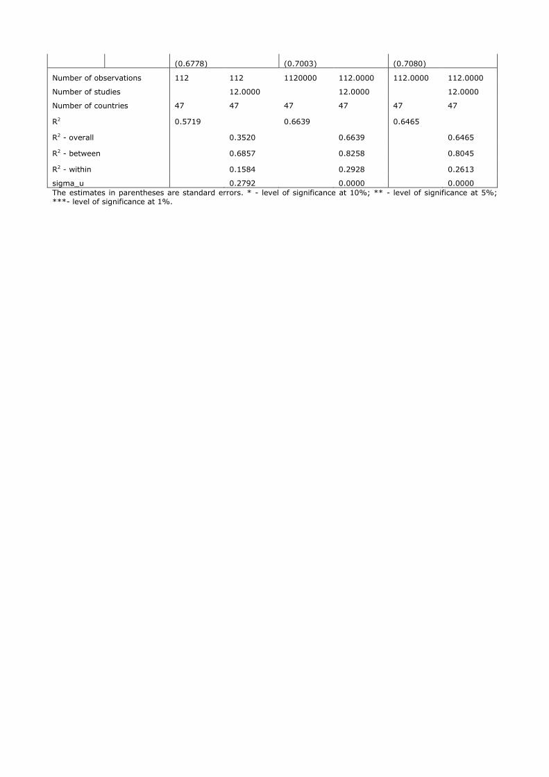
(0.6778) (0.7003) (0.7080)
Number of observations 112 112 1120000 112.0000 112.0000 112.0000
Number of studies
12.0000
12.0000 12.0000
Number of countries 47 47 47 47 47 47
R2 0.5719
0.6639 0.6465
R2 - overall
0.3520
0.6639 0.6465
R2 - between
0.6857
0.8258 0.8045
R2 - within
0.1584
0.2928 0.2613
sigma_u 0.2792 0.0000 0.0000
The estimates in parentheses are standard errors. * - level of significance at 10%; ** - level of significance at 5%; ***- level of significance at 1%.

List of figures
Figure 1. Map of Africa showing grouping of countries in the meta-sample into five sub
regions .............................................................................................................. 14
Figure 2. Kernel density plots of meta-sample with and without outliers for foods,
nutrients and calories .......................................................................................... 31
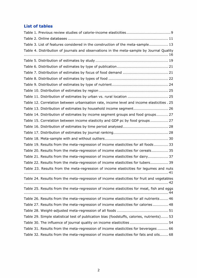
2
List of tables
Table 1. Previous review studies of calorie-income elasticities ..................................... 9
Table 2. Online databases .................................................................................... 11
Table 3. List of features considered in the construction of the meta-sample ................ 13
Table 4. Distribution of journals and observations in the meta-sample by Journal Quality
......................................................................................................................... 16
Table 5. Distribution of estimates by study ............................................................. 19
Table 6. Distribution of estimates by type of publication ........................................... 21
Table 7. Distribution of estimates by focus of food demand ...................................... 21
Table 8. Distribution of estimates by types of food .................................................. 22
Table 9. Distribution of estimates by type of nutrient ............................................... 24
Table 10. Distribution of estimates by region .......................................................... 25
Table 11. Distribution of estimates by urban vs. rural location .................................. 25
Table 12. Correlation between urbanisation rate, income level and income elasticities . 25
Table 13. Distribution of estimates by household income segment ............................. 26
Table 14. Distribution of estimates by income segment groups and food groups .......... 27
Table 15. Correlation between income elasticity and GDP pc by food groups ............... 27
Table 16. Distribution of estimates by time period analysed ...................................... 28
Table 17. Distribution of estimates by journal ranking .............................................. 28
Table 18. Meta-sample with and without outliers ..................................................... 30
Table 19. Results from the meta-regression of income elasticities for all foods ............ 33
Table 20. Results from the meta-regression of income elasticities for cereals .............. 35
Table 21. Results from the meta-regression of income elasticities for dairy................. 37
Table 22. Results from the meta-regression of income elasticities for tubers ............... 39
Table 23. Results from the meta-regression of income elasticities for legumes and nuts
......................................................................................................................... 41
Table 24. Results from the meta-regression of income elasticities for fruit and vegetables
......................................................................................................................... 42
Table 25. Results from the meta-regression of income elasticities for meat, fish and eggs
......................................................................................................................... 44
Table 26. Results from the meta-regression of income elasticities for all nutrients ....... 46
Table 27. Results from the meta-regression of income elasticities for calories ............. 48
Table 28. Weight-adjusted meta-regression of all foods ........................................... 51
Table 29. Simple statistical test of publication bias (foodstuffs, calories, nutrients) ...... 53
Table 30. The influence of journal quality on income elasticities ................................ 54
Table 31. Results from the meta-regression of income elasticities for beverages ......... 66
Table 32. Results from the meta-regression of income elasticities for fats and oils ....... 68
How to obtain EU publications
Our publications are available from EU Bookshop (http://publications.europa.eu/howto/index_en.htm),
where you can place an order with the sales agent of your choice.
The Publications Office has a worldwide network of sales agents.
You can obtain their contact details by sending a fax to (352) 29 29-42758.
Europe Direct is a service to help you find answers to your questions about the European Union
Free phone number (*): 00 800 6 7 8 9 10 11
(*) Certain mobile telephone operators do not allow access to 00 800 numbers or these calls may be billed.
A great deal of additional information on the European Union is available on the Internet.
It can be accessed through the Europa server http://europa.eu

2
doi:10.2791/661366
ISBN 978-92-79-54182-7
LF-N
A-27650
-EN
-N
JRC Mission
As the Commission’s
in-house science service,
the Joint Research Centre’s
mission is to provide EU
policies with independent,
evidence-based scientific
and technical support
throughout the whole
policy cycle.
Working in close
cooperation with policy
Directorates-General,
the JRC addresses key
societal challenges while
stimulating innovation
through developing
new methods, tools
and standards, and sharing
its know-how with
the Member States,
the scientific community
and international partners.
Serving society Stimulating innovation Supporting legislation