»STATISTIGAL INQUIRIES«Issued by »The Statistical Department«, Denmark

Income- enditure

Relations of Danish Wage

and Salary Earners

DrTDEPAR

By Erling Jørgensen

Published by »The Statistical Departmentein Collaboration with »The Institute of Statisticse

and »The Institute of Economics«of the University of Copenhagen

KØB E N HAVN

1965

PRINTED IN DENMARK BY AARHUUS STIFTSMOGTRYKKERIE A-S

CONTENTSList of tables VIIList of figures VIIIPrefaceChapter I. Background and main results

Ia. Background of the study 3Ib. Main results of the analysis 4Ic. The report 10

Chapter II. Review of the survey materiallia. Introductory remarks 12lIb. Concepts and methods of the survey 12

Collecting the information 12

Income and expenditure concept; unit of analysis 13

Period of the survey 15

Method of selection 15lic. Estimating mean values and their standard errors.

Accuracy of survey results 18

Processing of the material 19

Chapter III. Objectives of the analysis. Engel functionslila. Introductory remarks 22IlIb. Choice of model

Determinants of expenditure 22Engel curves and household survey data 23What, then can the results be used for 28

hIc. Use of estimated Engel curves on the macro level 29

Chapter IV. Methods of analysishVa. Introductory remarks 31IVb. Choice of Engel functions and specification of the variables

Criteria of selecting Engel functions 31Description of the functions selected 32Specification of the variables 33Zero-observations 36Grouping problems 38

IVc. Variance assumptionsGeneral remarks 40Testing the hypothesis V = 2 2 42

IVd. Calculation of estimates of parametersFour linear functions 45The log-normal distribution function 46

VI

IVe. Tests for goodness of fitThe tests used 48Test for number of runs and for length of run; the d-test 49The F-test 50The X2-test 52The coefficient of correlation 52

JVf. Planning the computation programme and carrying out the computation 52

Chapter V. Main resultsVa. Introductory remarks 56Vb. Examination of test-results 57

Coefficient of correlation, between calculated and observed values 57The X2-test 60The F-test 64The test for number of runs and for the longest run; the d-test 71

Summary of test-results 77Vc. Analysis of estimates of the parameters

Regression analysis versus two-way cross-tabulation 77Interpretation of main results 80Interpretation of the estimates of the slope of the regression line 81Are the Engel curves for different social groups identical? 85An important reservation 86Conclusions 88

Chapter VI. Further analysis. The concept of unit-consumers, multiple regressionanalyses, etc.

VIa. The unit-consumer concept 90VIb. Multiple regression analyses 100

Danish summary 111

Literature 117Index 119

Appendix A. Main results 123

Appendix B. Correlation coefficient between residuals of different expenditure items 174Appendix C. The basic material 181

Appendic D. Detailed list of expenditures separately for each of 13 main expenditureitems. 240

LIST OF TABLES1,1 Income elasticities for 13 expenditure items; average values for 12 groups of wage and

salary earners 7

II,! Average income, saving and expenditures in 1955 in kroner per household 20IV,! Values of income elasticity, e, and marginal propensity to consume, m, for five Engel

functions 33IV,2 Average coefficient of variation, separately for 13 expenditure items within each of 12

groups of wage and salary earners 44IV,3 x2-test for constancy of coefficients of variation 46IV,4 Parameter estimates in the three-parameter case of the function

log i = log x + log I + fi log y);. Higher public servants and salaried employeesin the Capital 55

V, i Correlation coefficients (R x 100) between observed and calculated expenditures 58V,2 x2-test 62V,3 F-test for linearity (ratio between variances "around" the regression and variances within

groups) 66V,4 N-test for number of runs 68V,5 1-test for the longest run 73

V,6 d-test for size and direction of deviations from the regression 74V,7 Number of significant test results among 12 groups of wage and salary earners. Signifi-

cance level 95% (x2, F, 1) and 5% (N, d) 76V,8 Gain of regression. Standard errors in the distribution of expenditures and in the distribu-

tion of deviations from the double logarithmic Engel function, log y a + b (log xlog x) 79V,9 F-test for parallelism of Engel curves 83

10 Calculated income elasticities for 13 expenditure items for each of 12 groups of wage andsalary earners 85

V,!! Average income elasticities for 13 expenditure items 89VI,! a Average expenditure per person on dwelling in certain income groups separately for

different types of household 93lb Average expenditure per person on fuel and light in certain income groups separately

for different types of household 93VI,! c Average expenditure per person on food in certain income groups separately for different

types of household 94VI,ld Average expenditure per person on tobacco in certain income groups separately for diffe-

rent types of household 94VI,! e Average expenditure per person on clothing in certain income groups separately for

different types of household 95VI,lf Average expenditure per person on footwear in certain income groups separately for

different types of household 95VI,!g Average expenditure per person on washing and cleaning in certain income groups

separately for different types of household 96VI,!h Average expenditure per person on durables, excl, vehicles, in certain income groups

separately for different types of household 96

VI,! i Average expenditure per person on personal hygiene in certain income groups separatelyfor different types of household 97

VI,lj Average expenditure per person on books, newspapers, etc. in certain income groupsseparately for different types of household 97

VI,lk Average expenditure per person on sports, holidays, hobbies in certain income groupsseparately for different types of household 98

VI,ll Average expenditure per person on transport incl, own car in certain income groupsseparately for different types of household 98

VI,! m Average expenditure per person on union fees, subscriptions etc. in certain income groupsseparately for different types of household 99

VI,ln Average »expenditure« per person on savings in certain income groups separately fordifferent types of household 99

VI,2 Correlation between each two of thirteen expenditure items 104

VI,3 The biggest positive and negative correlation coefficient separately for each group ofwage and salary earners 106

VI,4 The highest and lowest values of the correlation coefficient of deviations, separately foreach social group 108

VI,5 Unexplained variance in the regression analysis 110

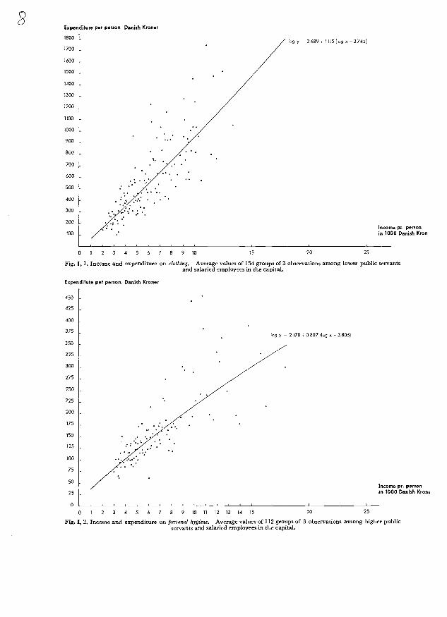
LIST OF FIGURES1,1 Income per person and expenditure on clothing. Average values of 154 groups of 3 ob-

servations among lower public servants and salaried employees in the capital 8

1,2 Income per person and expenditure on personal hygiene. Average values of 112 groupsof 3 observations among higher public servants and salaried employees in the capital 8

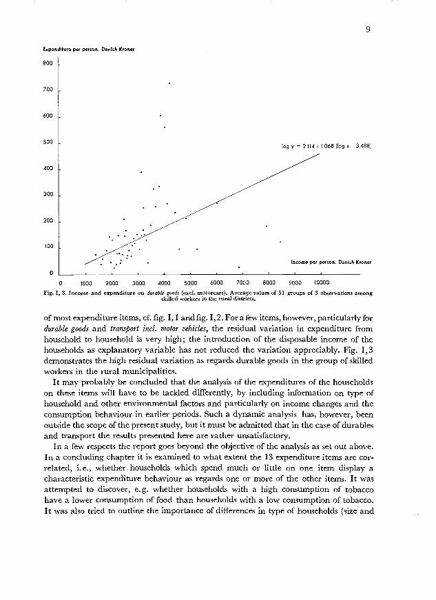
1,3 Income per person and expenditure on durable goods (excl, motorcars). Average values of51 groups of 3 observations among skilled workers in the rural districts 9

111,1 Expenditure on theatre and cinema 27

IV,! Two groups of expenditures on tobacco 37

IV,2 The variance of the expenditure on clothing plotted against the square of this expenditure 41

IV,3a Type of systematic deviations which will be revealed by the run tests, and may be not byother tests 50

IV,3b Type of systematic deviations which will be revealed by the F-test, but may be not bythe run tests 50

V, la Untransformed expenditure observations plotted against log x 64

lb Logarithmically transformed expenditure observations plotted against log x 64

V,2a Frequency of expenditure for given income 65

V,2b Frequency of log expenditure for given income 65

V,3 Five Engel functions. Income and expenditure on food. Skilled workers in the provincialtowns 81

V,4a Mean points for the twelve Engel curves for expenditures on books, newspapers etc 87

V,4b Mean points for the twelve Engel curves for expenditures on sports, holidays etc 87

1 Income and expenditure on sport, holidays and hobbies for four different types of house-holds 101

VI,2 Income and expenditure on food per person for four different types of households 101

PREFACEThe present analysis of the expenditure behaviour of Danish households of wage andsalary earners is essentially based on the model used by Prais and Houthakker in theiranalysis of a similar English material (The Analysis of Family Budgets, Cambridge,1955).

The scope of the analysis was determined by the Statistical Department, the Instituteof Statistics of the University of Copenhagen and the Institute of Economics of the Uni-versity of Copenhagen in concert. Mr. Kjeld Bjerke, lecturer, chief of division, the Sta-tistical Department, and the heads of the two institutes, Professor Anders Hald, dr. phil.,and Professor P. Nørregaard Rasmussen, dr. polit., having met regularly to discussproblems arising in the course of the work; this committee has also gone through thefinal report.

The day-to-day work was directed by Mr. Erling Jørgensen, cand, polit., The StatisticalDepartment, assisted for a brief period by Mr. Abling Thomsen, cand, polit., the StatisticalDepartment. Mr. Erling Jørgensen has also prepared the manuscript of the presentreport. Computations have been carried out by The Danish Institute of ComputingMachinery, the staff of which has rendered valuable assistance in the programmingprocess. Mrs. Lis Taxøe Jensen, the Statistical Department, has displayed great skilland care in preparing the many tabulations and examples to be used in the analysis.

The Translator of the Statistical Department, Mr. Vagn K. Sandberg, has translatedthe draft manuscript into English, and Mr. Niels Thygesen, cand, polit., has carriedout a terminological revision of this manuscript.

The expenditure in connection with the computations carried out by The DanishInstitute of Computing Machinery has been covered by a grant from the Danish StateResearch Foundation, and a grant has been received from the Rask-ørsted Foundationto cover the cost of the terminological revision of the manuscript. The expenditureincidental to the publishing of the book has been defrayed by the Statistical Department.

The analysis was started in the summer of 1959 and was concluded with a provisionalreport at the end of 1962.

Copenhagen 1964.

Chapter L

BACKGROUND OF THE STUDY ANDTHE MAIN RESULTS

I a. Background of the study.

The survey of income, consumption and saving patterns in 1955 of households of Danishwage and salary earners which was carried through at the beginning of 1956 is the mostcomprehensive and the most detailed of the consumption surveys undertaken by theDanish Statistical Department since it started making this kind of surveys in 1897').The primary object of the surveys was originally to procure information of the "Con-ditions of life in the different classes of society, including nutrition and consumption"2),but after the system of adjusting salaries, wages, benefits and other payments in accord-ance with a price index became generally adopted, the consumption surveys were pri-marily undertaken in order to provide the basic material for constructing a system ofweights to be used in the calculation of price indices. During recent years, however, thegenerally descriptive purpose, which was the primary one in the first consumption sur-veys, seems to be gaining ground again. One of the reasons for this development is thefact that it has been realized that the basic material which is obtained by means of aconsumption survey carefully planned and carried outin this connection the sub-stantial advances in survey techniques of the last decades should be borne in mind-provides information on essential economic relationships, particularly in connectionwith spending in relation to income, which cannot be illustrated so completely in anyother way3).

The Danish consumption survey for 1955 has, in fact, been subject to a more detailedprocessing than any of the previous surveys. Thanks to the scope and quality of the1955 survey it has been possible, through this detailed processing, to arrive at resultswhich are of direct interest to private institutions and persons as well as to public authori-ties.

A general outline of the 1955 survey, its planning and main results, was given in Sta-tistiske Efterretninger in 19574). Food consumption was dealt with separately in an article

')A complete list of publications on Danish consumption surveys will be found p. 118.Act concerning the Central Statistical Bureau 1895.Cf. I.L.O. (II).Statistiske Efterretninger 1957, No. 83.

4

in Statistiske Efterretninger in i 958). The data collected concerning the saving and personalwealth of the households of wage and salary earners were subject to a special analysis,the results of which were given in a volume of the series of Statistiske Undersøgelser in19606). Two volumes in the same series dealt with the data collected on the distributionand composition of the wage and salary incomes7).

The greater part of the information obtained from the households of wage and salaryearners concerned their consumption expenditure in the year 1955, and it was decidedto subject the consumption behaviour of these households to a more detailed analysis.It is the results of this study which are contained in the present publication.

I b. Main results of the analysis.

The analysis aimed at giving a precise description of the relationship between the dis-posable income of the Danish households of wage and salary earners and their expen-diture on some essential items in the year 1955. This relationship between disposableincome and the expenditure on given items is undoubtedly of considerable importancein helping to explain differences in consumption behaviour from one household toanother, although, of course, many other factors must be included if all such differencesare to be explained, such as type of household, residential and social classification, etc.However, the income-expenditure relationship is of great importance in another con-nection, namely for forecasting the development of consumption in response to givenchanges in income, for one household or group of households or for all households as awhole8).

The analytical work thus consisted mainly in deriving the best possible descriptionof the income-expenditure relationships. Such income-expenditure relationships oftengo by the name of Engel curves after the German economist and statistician, ErnstEngel9). More specifically, the work in connection with the analysis has consisted incalculating estimates of the parameters of five types of functions selected in advance andthen comparing these functions by means of a number of tests for goodness of fit inorder to find the Engel function most suitable for each expenditure item.

This is on the whole the same type of analysis as was adopted by J. S. Prais and H. S.Houthakker in their study of British family budgets from 195510). In fact, in many re-spects the present inquiry may be considered an application to Danish data of the ana-lytical tools which Prais and Houthakker present and discuss in their work.

Statistiske Efterretninger 1958, No. 46.Opsparing i lønmodtagerhusstandene 1955, Statistiske Undersøgelser, No. 3, Copenhagen 1960. (Sum-mary in English).Lønmodtagerindkomster, Fordeling og sammensætning, Statistiske Undersøgelser, No. 6, Copenhagen1962 and An Analysis of the Personal Income Distribution for Wage and Salary Earners in 1955.Statistical Inquiries, 1964.Cf. chapter III, p. 28, and Erling Jorgensen (10), pp. 54-61.Cf. Ernst Engel (10)PraisJ. S. and Houthakker H. S. (10)

5

Prais and Houthakker's study contains a discussion of alternative approaches to ana-lyses of budget data as well as a list of literature dealing with family budget studies11).These background problems, therefore, will not be elaborated here.

As regards the main lines of the present study a few points deserve mention in thissummary of methods and results.

To eliminate the most disturbing influences deriving from differences in the size ofthe households interviewed, all expenditure and income amounts were converted intoamounts per person for each of the 3100 households for which data were obtained.

The income concept used, which is the independent variable of the Engel curve, wasthen determined as disposable income (all cash receipts less paid personal taxes) perperson, and Engel functions were derived for 13 main expenditure items. In the appendixwill be found a detailed classification of these expenditures which together amount to85 per cent of total consumption expenditures for all households of wage and salaryearners. The 13 main items were the following:

DwellingFuel and lightingFood (incl, regular eating out, beer, wine, and liquor within the usual householdconsumption)TobaccoClothingFootwearWashing and cleaningDurable goods (excl, motor vehicles)Personal hygieneBooks, newspapers, etc.Sports, holidays, hobbies, etc. (incl, visits to restaurants, theatres, cinemas, andbeer, wine, and liquor outside the usual household consumption)Transport (incl, motor vehicles)Subscriptions, union fees, insurance premiums, etc. (excl, life and pension insurance)

The calculations were carried out separately for 12 groups of wage and salary earners,namely four social groups within each of the three regions of the country.

The three regions were the followingThe capital incl, suburbsThe provincial towns incl, suburbsUrban districts in the rural municipalities

In regions I and 2 the following social grouping was usedHigher public servants and salaried employeesLower public servants and salaried employeesSkilled workersUnskilled workers

11) Prais J. S. and Houthakker H. S. (10) p. 169.

6

In region 3, the urban districts in the rural municipalities, separate calculations werealso carried out for the social group of Agricultural workers. In this region no calculationswere carried out for the group of Higher public servants and salaried employees.

The five types of functions used were the following, x denoting disposable income perperson and y the expenditure per person on the item in question:

(1,1) log i = a + (log y - log ),(1,2) log=a+(v-'_i),(1,3) =a+,9(logvÏ),(1,4) = a + (v-1

(1,5) log = log x + log [1 (a + log y)]

a bar denoting average value and J (t) denoting the cumulative distribution functiont2

of the normal distribution (t)I

lV2

Considerable parts of the report on the analysis are devoted to a discussion of the esti-mation procedure so that it may be said that an evaluation of the methods of analysis wasanother main objective of the analytical work besides the calculation of the results of theanalysis.

The tests applied showed almost consistently that the double-logarithmic function (1,1)gave the best description of the Engel curve for all 13 expenditure items as a whole. Thisresult is in a way surprising because it implies that the income elasticity12) of the house-holds in their demand for each of the 13 commodity groups is constant over the incomerange (for given social group, since the calculations have, as mentioned, been carriedout separately for 12 groups of wage and salary earners). It might have been expectedthat commodity groups which are considered necessities in the higher income groupswould be regarded as luxuries in the lower income groups. This, however, is not con-firmed by the estimates of the income elasticities.

It might then be thought that this constancy of the income elasticity would hold goodonly in the case of the individual groups of wage and salary earners, which do not eachof them cover any wide income interval, but that the matter would be different if ailhouseholds were grouped together, in other words, that the estimates of should bedifferent for the different groups. However, there proves13) to be a remarkable stabilityas regards the mentioned estimate of , when we move from one group of wage andsalary earners to another. In the case of six expenditure items a hypothesis of constantincome elasticity through all 12 household groups can be maintained, and in the caseof the remaining 7 items the deviations, though statistically significant, are not verygreat. The demonstration of this stability in the income elasticity of the households in

Note that the income elasticity is identical with the parameter 1 in the double-logarithmic Engelfunction (I, 1).Cf. chapter V p. 83.

their expenditure on the most important items is one of the most conspicuous results ofthe analysis'4)

This stability renders it justifiable to calculate the average income elasticity for the12 groups of wage and salary earners for each of the 13 expenditure items. These averageelasticities are shown in table 1,1, where the expenditure items have been arrangedby size of the average income elasticity.

Table 1,1.Income elasticities for 13 expenditure items; average values for

12 groups of wage and salary earners.

7

It will be seen from this table that the expenditure items fall into three clearly definedgroups:

A group, which might be called necessities, in which the elasticity is just over 0.5,consisting of three items, food, footwear, fuel and lighting.

A second group, which might be called neutral commodities, with an elasticityclose to unity. This group includes 8 items, among which the two important items ofdwelling and clothing.

Finally, there is the third group, which might be called luxuries, in which theelasticity is significantly higher than unity; this group consists of the two items of transport(incl, motor vehicles) on the one hand and sports, holidays, hobbies, etc. on the other

As already mentioned, the main objective of the analysis has been to give a descrip-tion of the relationship between the income of the households of wage and salary earnersand their expenditures on important items. The analytical method employed, whichconsists chiefly in linear regression analysis, seems to yield satisfactory results in the case

14) This result invites the postulate that the income elasticities found for the population of wage andsalary earners have general validity for all population groups. Concerning the consequences of thispostulate, see Erling Jørgensen (12).

Item Average incomeelasticity

Fuel and lightingFootwearFood

0.510.560.61

Subscriptions, union fees, etc. 0.82Personal hygiene 0.86Washing and cleaning 0.86Dwelling 0.89Books, newspapers, etc. 0.98Tobacco 0.98Durable goods (excl, motor vehicles) 0.99Clothing 1.04

Transport (incl, motor vehicles) 1.39Sports, holidays, hobbies, etc 1.50

Expenditure per person. Danish Kroner

1800

1700

1600

1500

1400

1300

1200

1100

1000

900

800

700

600

500

400

300

200

100

log y = 2.689 . 1.115 (log o - 3.745)

0 1 2345678910 15 20 25

Fig. I, 1. Income and expenditure on clothing. Average values of 154 groups of 3 observations among lower public servantsand salaried employees in the capital.

Expenditure per person. Danish Kroner

log y -- 2178 0807 (log o -.3806)

0 1 2 3 4 5 6 7 8 9101112131415 20 25

Fig. 1,2. Income and expenditure on personal hygiene. Average values of 112 groups of 3 observations among higher publicservants and salaried employees in the capital.

Income Pr. personin 1000 Danish Kren

Income pr. personin 1000 Danish Krone

450

425

400

375

350

325

300

275

250

225

200

175

150

125

100

75

50

25

o

Expenditure per person. Dar'ish Kroner

9

log y = 2.114 -V 1.068 (log x - 3.488)

Income per person. Danish Kroner

0 1000 2000 3000 4000 5000 6000 7000 8000 9000 10000

Fig. I, 3. Income and expenditure on durable goods (excl, motorcars). Average values of 51 groups of 3 observations amongskilled workers in the rural districts.

of most expenditure items, cf. fig. I, i and fig. 1,2. For a few items, however, particularly fordurable goods and transport incl, motor vehicles, the residual variation in expenditure fromhousehold to household is very high; the introduction of the disposable income of thehouseholds as explanatory variable has not reduced the variation appreciably. Fig. 1,3demonstrates the high residual variation as regards durable goods in the group of skilledworkers in the rural municipalities.

It may probably be concluded that the analysis of the expenditures of the householdson these items will have to be tackled differently, by including information on type ofhousehold and other environmental factors and particularly on income changes and theconsumption behaviour in earlier periods. Such a dynamic analysis has, however, beenoutside the scope of the present study, but it must be admitted that in the case of durablesand transport the results presented here are rather unsatisfactory.

In a few respects the report goes beyond the objective of the analysis as set out above.In a concluding chapter it is examined to what extent the 13 expenditure items are cor-related, i.e., whether households which spend much or little on one item display acharacteristic expenditure behaviour as regards one or more of the other items. It wasattempted to discover, e.g. whether households with a high consumption of tobaccohave a lower consumption of food than households with a low consumption of tobacco.It was also tried to outline the importance of differences in type of households (size and

800

700

600

500

400

300

200

100

o

10

composition of household) to the consumption behaviour of households for given in-come classes.

As regards the first problemthe interrelationships of the 13 expenditure itemsthecalculations show only a slight correlation. Only in the case of the two items of dwellingand fuel and lighting was there a significant (positive) correlation. This result is a con-sequence of the design of the analysis, since the grouping of the many goods and servicesfor which information was obtained into a moderate number of main expenditure itemsaimed precisely at a grouping with only a slight positive or negative correlation betweenthe individual groups. This attempt to arrive at stable relationships between income anda few groups of expenditures at the same time ruled out a description of the consumptionbehaviour of the households towards individual goods and services; if such a descriptionwere to be attempted, the expenditure on other closely related goods and services wouldundoubtedly have to be taken into account.

As regards the importance of type and size of the household to the consumption be-haviour of the households, the examinations show that the size (i.e. number of persons)of the household was the dominant factor, and that the conversion into amountsper person from amounts per household eliminated the greater part of this "disturbing"influence. In the case of certain expenditure items, among them dwelling and tobacco,other influences made themselves felt; a general influence, as was to be expected, wasthe "economies of scale" effect, i.e. the expenditure per person falls as the number ofpersons per household rises.

I e. The report.

After this introductory survey of the background and plan of the analysis and of someof its main results, chapter II will present a review of the basic material. This review con-sists of a description of the practical work of carrying through the survey of consumptionand saving, i.e. the collection and processing of the basic material, and also a descriptionof the inaccuracy attaching to the figures derived from the basic material. Chapter IIalso contains a brief summary of average expenditure per household on the main expen-diture items. In chapter III the aim of the analysis will be defined, various models for ananalysis of the expenditure behaviour of the households being discussed, a discussionwhich concludes in a statement of the reasons for choosing the Engel curve approach asthe main subject of the analysis. Chapter IV contains a detailed discussion of the methodsof analysis. What types of functions are to be chosen as a basis for deriving Engel curvesfor the different expenditure items? How are the variables to be specified? How is thesuitability of the functions employed in the description of the income-expenditure rela-tionship to be tested?

In chapter V the results of the analysis are presented. The double-logarithmic Engelcurve was, according to the test made, found to be the "best" of the 5 types of functiontested.

Finally, chapter VI suggests examples of some further calculations which should make itpossible to achieve a more exhaustive description of the consumption behaviour of the

11

households than has been possible with the main tool of the present analysis, the Engelcurve. In order to explain the variations observed in the expenditures of the householdson a given item, differences in the size and composition of the households will be discussedas well as the expenditures of the households on one or more other items.

An appendix to the report contains partly the basic material and a detailed descriptionof the expenditure items comprised by each of the 13 main items and partly tablesshowing the results of the computations. These tables fall into two parts, the results ofthe main analysis, cf. chapter V and the results of the further calculations, cf. chapter VI.

A list of the literature used will be found on pages 117-118.

') Cf. references p. 118.

Chapter II.

REVIEW OF THE SURVEY MATERIAL

lia. Introductory remarks.

The pt esent analysis of the consumption patterns of Danish wage and salary earners in1955 is based on the family budget survey of households of Danish wage and salaryearners undertaken in 19561).

This survey comprised a total of 3100 households, selected by stratified samplingamong all households of wage and salary earners; the sampling procedure is decribedbelow.

The questionnaire used in the survey was very detailed as it was desirable to collectinformation on household expenditures for a large number of consumer goods cf. thedetailed list in the appendix p. 240. For the purpose of the present analysis, however, onlymain expenditure items are of interest as the emphasis of the analysis is on the consump-tion pattern as a whole rather than on consumption of individual commodities.

JIb. Concepts and methods of the survey.

1. Collecting the information.

The consumer survey has been carried through by personal interviews. This method hasbeen chosen in preference to the far cheaper one of mailing questionnaires to the house-holds for two reasons. Firstly because some of the questions were so complicatedthat the interpretation of an interviewer was considered necessary in order to ensurethat the households would understand them, and secondly to reduce the non-responserate to a minimum. Both as regards the quality of the information collected and asregards the response rate, gratifying results were achieved. Only 61 questionnaires outof a total of 3161 had to be rejected owing to unsatisfactory completion, and only 473households, or less than 12 per cent of all households approached, refused to cooperate.(Besides, 345 other households could not be contacted because of illness, change ofaddress, etc.).

The survey comprised income and assets of the household as well as its expendituresand savings during 1955, the expenditure being broken down into various items, andsaving being distributed by the various forms of saving.

13

Total saving, defined as net change in assets, was calculated on the basis of the figu-res for changes in debts payable and receivable in the course of the year. The interviewerchecked the figures against the difference between income and total consumption. Whereappreciable discrepancies were found, the household was contacted again, and sub-stantial errors in the figures for saving as well as in the various consumption items wereeliminated. On the whole, it may perhaps be concluded that both the interview methodand the fact that the total budget of the household was included in the survey havehelped in keeping what might be called errors of measurement at a minimum in thedata collected for consumption, saving and personal wealth.

2. Income and expenditure concepts; unit of analysis.

The purpose of the 1955 consumer survey was to illustrate expenditures and savings inhouseholds of wage and salary earners. Hence it follows directly that it is the householdwhich is the relevant unit of analysis both as regards consumption and saving. Thisgives rise to the problem of defining the household concept on which the survey was tobe based.

In drawing up such a definition there are two considerations to keep in mind. Firstly,the household should be defined in such a way that it contains thoseand only those-persons who behave as a unit both in relation to the earning of income (income unit)and to the spending of income (spending unit). Secondly, the household unit adoptedshould be practical for the purpose of selecting, collecting and processing the surveymaterial.

Without going into detailed definitional problems it should be emphasized that thesetwo considerations may in fact be irreconcilable. The consideration that the personsincluded in the household should act as one income and spending unit might lead to theselection of a household concept which will prove to be impractical in the selection ofthe sample or in the collection and processing of the material. Moreover, even if weinsist only on the point that the household should act as one income and spending unitwe are not assured of an unambiguous definition. Thus with regard to board and lodg-ing, domestic servants take part in the consumption of the household, but their incomesare not included in the joint income of the household. On the contrary, they are paidout of this income; domestic servants in some respects form part of the spending unit,but not of the income unit. If it is desired, e.g., to inquire into the relationship betweenthe income of the household and its food consumption, information supplied by thehouseholds in which there are domestic servants will give misleading results.

Further, it may be mentioned that the household concept which would be mostrelevant in an analysis of consumption, will not necessarily be the one that is mostrelevant in an analysis of saving, since it may very well be imagined that persons whoact as one unit as regards consumption will not make their saving decisions in common;examples are: households in which there are boarders and/or older children living athome who pay a certain amount towards the joint consumption of the household, butotherwise dispose independently of the rest of their income.

14

The household concept actually used was the following: those persons (and onlythose) who take part in the joint consumption, i.e., husband, wife, and children withoutan income of their own are included; also included were children living at home whohad incomes of their own and others who stayed permanently with the household,provided that these persons did not spend more than 50 per cent of their incomes outsidethe households.

As regards income, consumption and saving the following concepts were used:

Income:

Cash wages and salaries.Contributions to pension schemes withheld out of the salariesof public servants and salaried employees.Interest and Dividends.Pension, incl.old-age pension.Disablement pension.Contributions from separated or divorcedspouse.Unemployment relief.Contributions to housekeeping made by children andrelatives.Payment by lodgers for board and lodging.Amounts received under in-surance policies.Gifts.Inheritance, scholarships.Sales of motor car, moped, bi-cycle, furniture, clothing, etc.2) .Savings certificates received3).

Consumption expenditure:

Expenditures on purchases of all consumer goods, including all expenditures in con-nection with purchases of durable consumer goods (motor cars, motor cycles, furniture,household appliances, radio and television sets2), etc.), i.e. both initial payments ondurable consumer goods acquired in the course of the year and instalments on hire-purchase debt relating to acquisitions in this or previous years; taxes, subscriptions, etc.-Also cash contributions to relatives and gifts.

Saving:

Amounts spent on increasing, or received by reducing, the below-mentioned items:Cashin--hand.--Bank and savings bank deposits.Bonds and shares.Premium

bonds.Private mortgage deeds.Compulsory saving and savings certificates.-Value of real property.Business assets.Other assets.Life and deferred annuityinsurance (incl, contributions of public servants to pension funds).

Amounts spent on reducing, or received by increasing, the below-mentioned items:Debt to bank and savings bank not secured by mortgage in real property.Mortgage

debt in real property.Other debt apart from hire-purchase debt, etc.Only a few comments are necessary in connection with these definitions. As mentioned

above, saving was calculated also as the difference between income and consumptionin the course of the year. Since this method of calculation must, of course, give the sameresult as the calculation according to the above definition4)if the figures are correct

In the case of purchases of motor vehicles, the value of any motor vehicle traded in has been setoff against the value of the new vehicle.In connection with the imposing of new indirect taxes in 1955 saving bonds were issued to all per-sons with assessed income of kr. 4000 or more. The face value of the bonds was increasing with in-creasing income of the persons concerned.Cf. Statistiske Undersøgelser, No. 3, Opsparing i Lønmodtagerhusstandene. 1955, Copenhagen1960, pp. 11-16.

15

the interviewers were able to get a good check on the data collected by comparingthe amounts of saving resulting from the two definitions.

Besides, it should be emphasized that the definitions used are based on a "cash pointof view". Income comprises all cash payments to the household, incl, gifts and amountsreceived under insurance policies. On the other hand, consumption contains, as a generalrule, all amounts actually paid by the household; this involved, for instance, that inthe case of purchases of durable goods, only the initial cash payment and any instalmentspaid during the survey period were included.

Period of the survey.

In the choice of survey period two conflicting considerations have to be taken into account.Firstly, it is desirable that the households interviewed should be able to remember, atthe time of the interview, the size of their income during the survey period and, in parti-cular, how they have spent this income. For this reason, it would be desirable to haveas brief a survey period as possible. On the other hand, however, it is desirable thataccidental fluctuations should not be allowed to have too much influence on the results,neither as regards the income earned nor as regards the spending of it. If both the earningof the income and the consumption took place at a regular rate, this consideration wouldnot give rise to any problems, but since particularly some consumption expendituresoccur irregularly, it would be reasonable to make the survey period so long that theseirregularities will be smoothed out. Since seasonal factors must be presumed to play adominant part in these fluctuations, it was found reasonable to use the year as the sur-vey period.

Especially as regards income earned experience shows that most households will havea precise idea of it only for a period of one year and only once a year, namely when theyfill in their income tax returns. Therefore the survey was carried out immediately afterthe date for delivering of the income tax returns, viz, the 1st of February.

Method of selection.

The selection of a sample of basic sampling units on the basis of probability theory (i.e.,in such a way that it becomes possible to calculate the standard error of the results)requires, firstly, a specification of the population from which the sample is to be drawn(setting up a frame for the selection), and secondly, the choice of a sampling design basedon random selection (i.e., a selection by which all the elements of the population havea specified probability of being selected).

As regards the setting up of a frame for the consumer survey, the population census onthe 1st October, 1955, provided a complete "list" of all households in Denmark. In view ofthe main object of the survey, which was an analysis of the consumption patterns ofhouseholds of wage and salary earners, it was decided to exclude from the frame allrural municipalities without urban areas because there are very few wage and salaryearners in those municipalities. The few wage and salary earners who were to be foundthere were considered to be represented by the households of wage and salary earners

16

selected in the rural minicipalities with urban areas. The frame was accordingly thosehouseholds in the whole of Denmark, except in the "purely" rural municipalities,which were recorded in the population census schedules as having a wage or salaryearner as head of household.

The choice of sampling design was influenced by a number of factors, the most importantof which will now be briefly discussed.

The guiding principle in the considerations which preceded the choice of samplingdesign was that the standard error of the estimates calculated on the basis of the sampledrawn should be below a certain limit, and that the costs of the survey should be heldat a minimum given this maximum standard error5).

However, the sampling design which gives the lowest standard error for one of theestimates, e.g. for total food consumption expenditure per household, will not always at thesame time give the lowest standard error for all the other estimates. As soon as a surveyis to form the basis of a calculation of several estimates, it is therefore necessary to specifyone of the quantities which it is desired to estimate on the basis of the sample as thedecisive one in the choice of sampling design. One may then hope that this design willalso be favourable as regards the other quantities to be estimated. Alternatively, all thequantities to be estimated must be arranged by order of priority and an overall evalua-tion must be made for the purpose of arriving at a design which minimizes the sum ofthe standard errors for all the quantities estimated, the individual standard errors beingassigned weights corresponding to their order of priority.

One of the objects of the 1955 survey was to provide the basis for calculating a systemof weights for the Danish price index. Therefore the estimation of average expenditureon the main items of goods and services which are covered by the price index wereassigned a high priority. As estimates made on the basis of preceding consumer survey(1948) showed that there was a high correlation between the total expenditure of ahousehold and expenditures on certain main items, the desired end was assumed to beattained by fixing certain limits of the standard error for the total expenditures perhousehold for each of twelve groups of wage and salary earners6).

Ina following section an account will be given of the calculation of these standard errors.With the mentioned point of departure (that the survey should be planned with a

view to minimizing the standard error for the total consumption expenditure), the sampl-ing design was otherwise determined by a number of practical and theoretical considera-tions.

Firstly, already the choice of method of enumeration places certain restrictions onthe sampling procedure. The decision to carry through the survey by means of inter-viewers who are to call on each sample household up to six times, makes it natural toassign to each interviewer as many households as he is able to call on within the periodof the survey. This procedure ensures that interviewers gain a maximum of experiencein taking interviews. It may also be mentioned that the possibilities of supervision forthe central authorities will be considerably reduced if there are too many interviewers.

See E. Lykke-Jensen: (13), pp. 16-18.Viz, four social status groups separately within three district categories; cf. below p. 34.

17

Consequently, it was desirable that the households should be selected in clusterswithin geographical areas, whereby the transport costs of the interviewers would beconsiderably reduced. Each cluster corresponds to the capacity of one interviewer, inthis survey approximately twenty households.

Besides, the very form of the frame will play a part in the considerations concerningthe method of selection. In this case, as already mentioned, the schedules from the 1955population census provided the frame from which the sample was drawn, and as theseschedules are arranged by municipalities (in Copenhagen by "roder" (tax collectiondistricts), in Frederiksberg and Gentofte by parishes), it seemed natural to base thesampling on whole municipalities (parishes or "roder"). As it was possible to groupthese municipalities in accordance with the criteria which were considered relevant tothis inquiry, viz, distribution by industry and degree of urbanization, it was foundreasonable to use stratified sampling. Finally, the desirability of illustrating the con-sumption patterns of the individual social status groups separately within each of thethree district categories, (the capital, provincial towns with suburbs, and rural muni-cipalities 'with urban areas) made it natural to conduct the survey in such a way thatit would be possible to calculate separate estimates for each status group within thesethree district categories.

The result of these considerations was accordingly that the sampling was made intwo stages within each of the three mentioned district categories. At the first stage muni-cipalities ("roder", parishes) were drawn by random selection from strata of uniformmunicipalities already formed, the probability of selection of each municipality ("rode",parish) being proportionate to the number of households in the municipality. Actually,the selection ought to have been made in proportion to the number of households ofwage and salary earners, but this number was unknown. As the households of wage andsalary earners constituted a more or less constant share of the total number of house-holds within each stratum of municipalities this procedure seems permissible. At thesecond stage households of wage and salary earners (basic sampling units) were drawnfrom each municipality in the first stage sample of municipalities, households belong-ing to different status groups7) drawn with different probability.

In the capital 16 first stage units were selected, comprising about 36000 householdsof wage and salary earners, from which were drawn 1262 second stage or final units,i.e. individual households. In the provincial towns the numbers of first and secondstage units were 17 and 920 respectively, the sample of first stage units comprising about85000 households. In the rural districts the numbers were 26, 918 and about 4000 re-spectively. Whereas the final sample of 3100 basic sampling units comprised only about0.45 per cent of all households of wage and salary earners, the number of such house-holds in the first stage sample of municipalities comprised about 18 per cent of the totalnumber8).

Finally, it should be mentioned that the definition adopted of the basic unit of ana-lysisall members of the expenditure unitdid not quite correspond to the units

Higher salaried, lower salaried, skilled and unskilled, cf. p. 5.A similar approach was used in the Danish labor force surveys in 1951 and 1952, cf. The DanishLabor Force Surveys. Statistical Review, New-Series vol. 2, No. 7, pp. 259-267.

18

selected at the second stage (the sampling units), as these units had been determinedby the choice of the frame of the survey, namely the schedules from the 1955 populationcensus. Since, according to the definition used in the population census, the householdcomprises all persons staying permanently in the household, with the exception oflodgers providing their own food, whereas in the consumer survey the household com-prises only the persons who contribute at least fifty per cent of their income towardsthe consumption of the household9), the population census household will in some casescomprise more persons than the basic sampling unit of the consumer survey. This factleads to certain complications in estimating averages for the whole country and alsoin estimating the true standard errors of these averages, but in the following this hasnot been taken into account as we have assumed that the inaccuracy introduced hereby isinsignificant compared with the inaccuracies which arises in the course of the collectionand processing of the questionnaires

lic. Estimating mean values and their standard errors.

1. Accuracy of the results of the survey.

The estimates based on the 1955 consumer survey are subject to a ceitain degree ofinaccuracy. This inaccuracy consists of two components. The first originates in the col-lection and processing of the material, i.e., wrong or inadequate information, errors incoding and punching, etc. The errors of this type are often called systematic errors(bias), cp. the following section. The other component is called sampling error, and itoccurs because only a sample of households and not the entire population is observed.

As the sample of households of wage and salary earners has been selected by strati-fied two-stage sampling, the sampling error of the estimates for each of the twelve groupsof wage and salary earners will consist of two elements; firstly, the error due to thevariation, within strata, among the sampling units at the first stage, municipalities,and secondly the error which is due to the variation among the sampling units at thesecond stage, i.e., among the individual households within municipalities.

While it is impossible to arrive at more precise estimates of the systematic errors, thesampling method adopted makes it possible to form estimates of the two elements ofthe sampling error10).

The calculation have shown that the error element due to variation among individualhouseholds within municipalities is dominant.

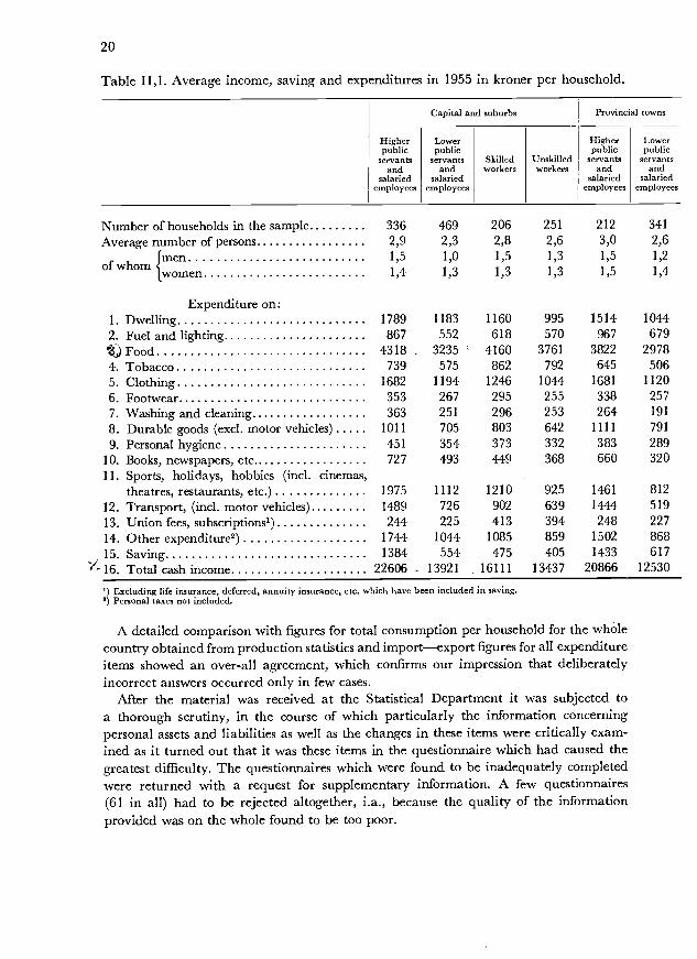
Table 11,1 shows estimates of average expenditure per household for 14 expendi-ture groups; the table shows also the average saving and cash income per householdfor each of the twelve groups of wage and salary earners. The standard sampling errorof the estimated total expenditure per household is estimated at kr. 140 or approximatelyi per cent of the total expenditure; 70 per cent of the standard error is due to variationbetween households within first-stage sampling units.

S) Cfr. the exact definition, p. 14 above.10) Cf. Statistiske Undersøgelser No. 3, Opsparing i lønmodtagerhusstandene 1955, Copenhagen 1960,

pp. 3-4.

") Cf. Prais S. J. and Houthakker H. S. (10) p. 42.

19

In the regression analyses which form the greater part of the present inquiry the ob-servations for each of the twelve groups of wage and salary earners into which the 3100households observed have been divided, have been treated as deriving from a simplerandom selection. The estimates of the standard errors of the parameter estimates willtherefore become a little too high since the stratification effect is ignored, and besides,some bias may be expected to occur in the estimation of the parameters because thedeviation of the observations from the regression line is evaluated on an assumption ofsimple random selection, whereas the actual procedure is two-stage stratified sampling,cf. chapter 3, page 23. Howewer, this bias must be considered insignificant in relationto the total variance in the distribution of the deviations from the regression line of theobservations.

2. Processing of the material.

The inaccuracy of the estimates, discussed above, refers only to the sampling error, i.e.,the error which will inevitably occur when estimates for the whole population are tobe made on the basis of a sample of the population. With a given standard deviationin the distribution of the elements of the population the sampling error depends on thesize of the sample and the sampling methods; it has been attempted, within the givencost framework, to make this sampling error as small as possible.

However, the estimates can also be subject to another type of error, which also occursin complete enumerations, namely the so-called systematic errors, i.e., errors causedby wrong or inadequate completion of questionnaires and from the processing of thematerial, that is, errors in the scrutiny, coding and punching of the material received.

In the paragraph above on the enumeration method it was mentioned that the sur-vey was conducted through interviews, partly to induce the sample households to co-operate, and partly to reduce the number of wrong answers. The 160 interviewers hadreceived thorough instruction concerning the survey through letters and at speciallessons at which officers from the Statistical Department went through the problemsin connection with the completion of the questionnaires A provisional scrutiny of theanswers could therefore be made by the interviewers themselves at the time of the inter-view, the interviewers making a rough comparison of incomes and expenditures. Incases of discrepancy the interviewer was to take care that the household interviewedprovided, whereever possible, the necessary supplementary information. There is reasonto believe that thereby more correct figures have been obtained for the size of incomeand for items of expenditure which people might otherwise fail to state correctly.

It is obviously extremely difficult to indicate, even with rough approximation, themagnitude of errors which have arisen owing to people giving wrong answers to theinterviewer. Experience from similar surveys abroad supports a belief that such incor-rect statements are particularly frequent within the field which is often designated con-spicuous consumption, i.e., such items as tobacco, liquor, consumption in restaurants,etc").

20

Table 11,1. Average income, saving and expenditures in 1955 in kroner per household.

S) Excluding life insurance, deferred, annuity insurance, etc. which have been included in saving.) Personal taxes not included.

A detailed comparison with figures for total consumption per household for the wholecountry obtained from production statistics and importexport figures for all expenditureitems showed an over-all agreement, which confirms our impression that deliberatelyincorrect answers occurred only in few cases.

After the material was received at the Statistical Department it was subjected toa thorough scrutiny, in the course of which particularly the information concerningpersonal assets and liabilities as well as the changes in these items were critically exam-ined as it turned out that it was these items in the questionnaire which had caused thegreatest difficulty. The questionnaires which were found to be inadequately completedwere returned with a request for supplementary information. A few questionnaires(61 in all) had to be rejected altogether, i.a., because the quality of the informationprovided was on the whole found to be too poor.

Higherpublic

servantsand

salariedemployees

Lowerpublic

servantsand

salariedemployees

Skilledworkers

Unskilledworkers

Higherpublic

Servantsand

salariedemployees

Lowerpublic

Servantsand

salariedemployees

Number of households in the sample 336 469 206 251 212 341

Average number of persons 2,9 2,3 2,8 2,6 3,0 2,6Imen 1,5 1,0 1,5 1,3 1,5 1,2

of whomIwomen 1,4 1,3 1,3 1,3 1,5 1,4

Expenditure on:1. Dwelling 1789 1183 1160 995 1514 1044

2. Fuel and lighting 867 552 618 570 967 679()Food 4318 3235 4160 3761 3822 29784. Tobacco 739 575 862 792 645 506

5. Clothing 1682 1194 1246 1044 1681 1120

6. Footwear 353 267 295 255 338 2577. Washing and cleaning 363 251 296 253 264 191

8. Durable goods (excl, motor vehicles) 1011 705 803 642 1111 791

9. Personal hygiene 451 354 373 332 383 28910. Books, newspapers, etc 727 493 449 368 660 32011. Sports, holidays, hobbies (incl. cinemas,

theatres, restaurants, etc.) 1975 1112 1210 925 1461 812

12. Transport, (incl, motor vehicles) 1489 726 902 639 1444 519

13. Union fees, subscriptions') 244 225 413 394 248 227

14. Other expenditure2) 1744 1044 1085 859 1502 868

15. Saving 1384 554 475 405 1433 617

"16, Total cash income 22606 13921 16111 13437 20866 12530

Capital and suburbs Provincial towns

21

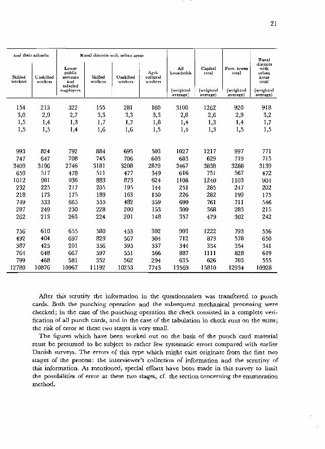
After this scrutity the information in the questionnaires was transferred to punchcards. Both the punching operation and the subsequent mechanical processing werechecked; in the case of the punching operation the check consisted in a complete veri-fication of all punch cards, and in the case of the tabulation in check runs on the sums;the risk of error at these two stages is very small.

The figures which have been worked out on the basis of the punch card materialmust be presumed to be subject to rather few systematic errors compared with earlierDanish surveys. The errors of this type which might exist originate from the first twostages of the process: the interviewer's collection of information and the scrutiny ofthis information. As mentioned, special efforts have been made in this survey to limitthe possibilities of error at these two stages, cf. the section concerning the enumerationmethod.

and their suburbs Rural districts with urban areas

All Capital Prov. towns

Ruraldistricts

withLowerpublic Agri- households total total urban

Skilled Unskilled servants Skilled Unskilled cultural areasworkers workers and

salariedemployees

workers workers workers

(weightedaverage)

(weightedaverage)

(weightedaverage)

total

(weightedaverage)

154 213 322 155 281 160 3100 1262 920 9183,0 2,9 2,7 3,3 3,3 3,3 2,8 2,6 2,9 3,21,5 1,4 1,3 1,7 1,7 1,8 1,4 1,3 1,4 1,71,5 1,5 1,4 1,6 1,6 1,5 1,4 1,3 1,5 1,5

993 824 792 884 695 503 1027 1217 997 771747 647 708 745 706 603 683 629 719 715

3409 3196 2746 3181 3208 2879 3467 3838 3288 3139659 517 478 511 477 349 616 751 567 472

1012 981 936 883 873 624 1108 1240 1103 904232 225 217 205 195 144 251 285 247 202218 173 175 189 163 150 226 282 199 175749 533 665 555 482 359 690 761 711 546287 249 230 228 200 153 300 368 283 215262 213 263 224 201 148 357 479 302 242

756 610 655 580 453 302 903 1222 793 556492 404 697 829 567 304 712 873 578 650387 425 201 356 395 337 344 334 354 341764 648 667 597 551 366 887 1111 828 619799 468 581 352 562 294 635 626 703 555

12780 10876 10967 11192 10253 7743 13569 15810 12934 10928

Chapter III.

OBJECTIVES OF THE ANALYSIS. ENGEL FUNCTIONS

lila. Introductory remarks.

The basic material available from the 1955 consumer survey is, as mentioned above,very comprehensive. For each of the 3100 households included in the survey approx-imately fifty punch cards (80 columns) were prepared. A complete description of thismaterial, including an analysis of the relationships among the many quantities of whichit is made up, is naturally out of the question. In order to keep the analytical workwithin reasonable limits, it is necessary to concentrate on some essential, well-definedproblems. More precisely: among the many possible models which could be tested bymeans of this material, a few are to be selected which are of substantial interest fromthe points of view of economic theory, social policy, etc. The analysis then consists inconfronting these models with the information collected.

From the point of view of economic theory, interest would focus on a model capableof explaining the consumption expenditures of households as a function of quantitiesfamiliar from economic theory as determinants of consumer behaviour. Hereby it might bepossible to evaluate consumption, once information on those quantities to which it isfunctionally related becomes available. If the quantities in question may be more con-fidently predicted than consumption itself, such functional relationships will be usefulin predicting consumption.

From the point of view of statistical theory the greatest interest will attach to esti-mation procedures; how are the best estimates of the parameters in the chosen modelsto be computed? What tests are applicable for purposes of comparing the estimates?

The computional work involved in the analysis has been carried out on an elec-tronic computer. Accordingly it has been possible to choose more labour-consumingmodels and methods of calculation than if only the traditional calculating facilities hadbeen available.

IlIb. Choice of model.

1. Determinants of expenditure.

According to traditional economic theory the expenditure of a household on a givencommodity is determined primarily by the income of the household and by the priceof the item in question. Prices of other commodities, expenditure of the household onother commodities as well as expenditure of other households on this and other commodi-

23

ties may also appear as important arguments. Other factors are of course, the compositionof the household, its geographical location and social status. Also previous income andincome change of the household as well as its assets might play an important role indetermining the consumption behaviour.

As the present analysis is based upon a consumer survey relating to a given point oftime and a given market, prices may be considered constant, independent of othervariables as e.g. income and expenditure. All other variables mentioned above, however,can be found in the basic material of this inquiry, and if it was possible to set up a simplemodel of the relationships of these variables the parameters of such a model might beestimated.

However, there is no presumption that the relationships between the variables aresimple at all. If the analysis is to be practicable, a relatively simple type of functionmust be chosen and the number of variables must be further reduced. Of the quantitiesmentioned above there is a strong presumption that household income is dominant inthe determination of the expenditure pattern, while the household expenditure on othercommodities plays a less prominent part, cf. chapter VI, p. 110. Therefore, it we furtherdisregard income changes and assets as well as household expenditure on other commo-dities (and the consumption pattern of other households), a relationship remains withingiven social groups of households containing solely the two variables expenditure of thehousehold and its income.

In a discussion of the relationship between these two quantities it is natural to startby emphasizing that expenditure is in the nature of a dependent variable to income,while income may reasonably be considered an independent or a determining variablecf. Prais & Houthakker (10) p. 80. It is quite obvious, however, that very often there isan influence the other way round, planned or incurred expenditures determining tosome extent the income-earning behaviour of the household. On the whole this influencemay be considered weak as compared to the influence of income on expenditure andespecially as regards households of wage and salary earners as their possibilities forincreasing income in the short run are rather limited.

Assuming that all households (household size and composition, social and geographicalgroup held constant) show identical income-expenditure relationships except for randomvariation, a description of the "average" household of wage and salary earners will beof the form

(111,1) y = f (x) +

where y denotes household expenditure on a given item, x the household income andL the effects on y from omitted determining variables plus random effects.

2. Engel curves and household survey data.

Formula (111,1) is the general expression of the Engel curve for a given expenditureitem indicating the relationship between a household's income and its expenditure onthat item. It was decided to place the Engel curve in the centre of the analysis, and thegreater part of this and the following chapter is therefore devoted to a discussion of

24

methods of determining parameters in Engel functions by means of a household budgetsurvey material.

Before discussing the question of the type of Engel functions a few remarks shouldbe made in connection with the general approach of the analysis, which is indicatedby the choice of the Engel curve as the main object of investigation.

Is it at all possible conceptually to estimate Engel curves on the basis of householdbudget surveys? Or stated more precisely: Assuming that all information in a surveyprovides reliable measurements of the incomes and expenditures of a number of indi-vidual households in the population group investigated, is it then possible to estimatetrue Engel curves based on that survey? Obviously, the degree of interest which wouldattach to the analysis from the point of view of economic theory depends very muchon the answer to this question.

It is important to realize from the outset that our basic material does not allow ofany direct testing of an Engel function relating to an individual household. For a givenhousehold only one set of income and expenditures is known, whereas several differentsets of such observations would be necessary to enable us to test any hypothesis concerningthe income-expenditure relationships of this household.

However, it may be possible to make up for this defect by inserting observations ofthe expenditures of other households on the commodity, these other households beingselected in such a way that the relevant values of the income scale will be represented.Thus, instead of studying each household's expenditure reaction to various income levels,the relationship between the expenditures and incomes of many different householdsfor one period is studied and it is postulated that by doing so the Engel curve of the"average" household in 1955 as written in (111,1) above will be obtained.

On the face of it, this postulated Engel curve is merely a description of the incomesand expenditures of various households. Such a description is, of course, valuable initself since it enables us to make a statement of the following form: in the Danish popu-lation of wage and salary earners in 1955, households with an income of x1 kr. spent anaverage of fj (x1) kr. on the i'th commodity, and households with an income of x2 kr.spent fj (x2) kr. apart from random deviations. Obviously the significance of the ana-lysis as seen from the viewpoint of economic theory will be higher if this description ofthe income and the expenditure on certain commodities or groups of commodities of3100 households will be a useful approximation to the Engel curves for the Danishpopulation of wage and salary earners in 1955.

The Engel function, as defined in (111,1), is static, i.e., it gives an expression for theexpenditure behaviour which the "typical" household will display, ceteris paribus, atalternative levels of income after any initial adjustment processes have been completed.This function, accordingly, entirely disregards the time factor and also the processwhereby the households passes from one income level to the other. More concretelythis process might be exemplified as follows: a household whose income rises will notadjust its expenditure behaviour to the new income level until some time has passed;hereby the saving of this household may temporarily be higher than the average forhouseholds whose incomes are permanently on this higher level. Conversely, a house-hold which passes from a higher to a lower income will try to maintain consumption-

25

thereby reducing savingthan the average for households whose incomes are permanentlyon this lower level. Furthermore, the related 'more general' question arises whether thereaction of an individual household to changes in income will depend on income andconsumption changes in neighbouring households').

These and other dynamic elements in the consumption behaviour of the householdshave been left out of account in the Engel functions of the type shown in (111,1)butthey are included in the estimates of the income-expenditure curve which can be madefrom the observations of the 3100 households in the basic material, and probably insuch a way that the estimates are influenced systematically. It is thus highly probablethat among the high-income households in the survey there will be relatively manywho have experienced an appreciable increase in income since the immediately pre-ceding period, while, conversely, there will be relatively many households withdeclining incomes at the lower end of the scale. The consumption expenditures observedfor the high income groups will therefore tend to understate the "true" (static) propen-sity to consume, while among the low income groups the "true" propensity to consumewill be lower than the observed expenditures, i.e., the Engel curve which is estimatedwill rise more slowly than a "true", static Engel curve.

The postulate: that the observed relationships between income and expenditure forthe 3100 households in 1955 are identical with the Engel curves as defined by (111,1)has, however, other weaknesses.

It does not allow for the dependence of the individual household on the consumptionbehaviour of other households. That such interdependence among the consumptionexpenditures of the individual households exists has long be recognized in demandtheory2). The Engel curve is based on a ceteris paribus assumption and answers ques-tions of the type: what amount would a household spend on the i'th commodity if itsincome rises by kr. 1000, kr. 2000, etc., assuming that the other factors in the household situ-ation are unchanged? The most important factors here are: household size, residence,social status and the relative income position of the household in relation to its "neigh-bours". The curves we can estimate from the available observation material, however,refer to households with, frequently, highly deviating environmental factors, and inobservations of expenditures for households at different income levels it is thereforeimpossible to maintain the mentioned ceteris paribus assumption. We may assume thatexpenditures on durable goods are highly susceptible to the influence of environmentalfactors, whereas, e.g., the expenditure on typical necessaries is less dependent on theconsumption behaviour of other households.

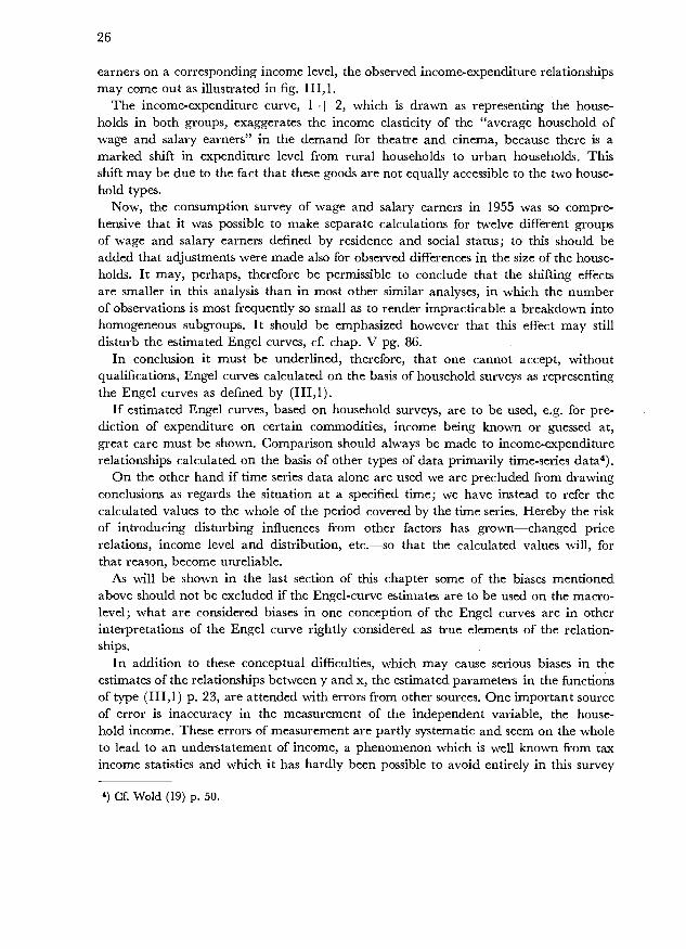
The so-called layereffect3), may also lead to a wrong evaluation of the "true" Engelcurve. If, e.g., we imagine that wage and salary earners in the rural districts, who are onan average at a lower income level than wage and salary earners in the towns, have aconsiderably lower expenditure on theatre and cinema than urban wage and salary

Cf. Duesenberry, J (3), Friedman, M. (7), Modigliani, F. (15) for a theoretical discussion of thisaspect of the consumption pattern; Danish empirical studies on the subject are found in Opsparing ilønmodtagerhusstandene 1955, Copenhagen 1960.Cf. Duesenberry, J. (3), Friedman, M. (7), Stone, R. (17).

2) Cf. WoId (19) p. 68.

26

earners on a corresponding income level, the observed income-expenditure relationshipsmay come out as illustrated in fig. 111,1.

The income-expenditure curve, I + 2, which is drawn as representing the house-holds in both groups, exaggerates the income elasticity of the "average household ofwage and salary earners" in the demand for theatre and cinema, because there is amarked shift in expenditure level from rural households to urban households. Thisshift may be due to the fact that these goods are not equally accessible to the two house-hold types.

Now, the consumption survey of wage and salary earners in 1955 was so compre-hensive that it was possible to make separate calculations for twelve different groupsof wage and salary earners defined by residence and social status; to this should beadded that adjustments were made also for observed differences in the size of the house-holds. It may, perhaps, therefore be permissible to conclude that the shifting effectsare smaller in this analysis than in most other similar analyses, in which the numberof observations is most frequently so small as to render impracticable a breakdown intohomogeneous subgroups. It should be emphasized however that this effect may stilldisturb the estimated Engel curves, cf. chap. V pg. 86.

In conclusion it must be underlined, therefore, that one cannot accept, withoutqualifications, Engel curves calculated on the basis of household surveys as representingthe Engel curves as defined by (111,1).

If estimated Engel curves, based on household surveys, are to be used, e.g. for pre-diction of expenditure on certain commodities, income being known or guessed at,great care must be shown. Comparison should always be made to income-expenditurerelationships calculated on the basis of other types of data primarily time-series data4).

On the other hand if time series data alone are used we are precluded from drawingconclusions as regards the situation at a specified time; we have instead to refer thecalculated values to the whole of the period covered by the time series. Hereby the riskof introducing disturbing influences from other factors has grownchanged pricerelations, income level and distribution, etc.so that the calculated values will, forthat reason, become unreliable.

As will be shown in the last section of this chapter some of the biases mentionedabove should not be excluded if the Engel-curve estimates are to be used on the macro-level; what are considered biases in one conception of the Engel curves are in otherinterpretations of the Engel curve rightly considered as true elements of the relation-ships.

In addition to these conceptual difficulties, which may cause serious biases in theestimates of the relationships between y and x, the estimated parameters in the functionsof type (111,1) p. 23, are attended with errors from other sources. One important sourceof error is inaccuracy in the measurement of the independent variable, the house-hold income. These errors of measurement are partly systematic and seem on the wholeto lead to an understatement of income, a phenomenon which is well known from taxincome statistics and which it has hardly been possible to avoid entirely in this survey

4) Cf. Wold (19) p. 50.

Expenditure

2. rural households

Fig. III, 1. Expenditure on theatre and cinema.

either5). The occurence of inaccuracy in the independent variable even if there is nosystematic error of measurement, leads to a systematic error in the evaluation of theslope of the regression lines. If the amount of inaccuracy can be estimated, it will bepossible to adjust for it in the evaluation of the slope6), but this is not possible in ourcase, and the mentioned adjustment therefore cannot be made.

One of the requirements for determining unbiased estimates of the parameters of anEngel function of the form (111,1) by means of the regression analysiswhich will bethe main tool in the followingis that this function is specified in such a way that e isindependent of x. This involves either (1) that x is a quantity given in advance andaccordingly not subject to variation in our experimental set-up, or (2) that any variationin x is independent of e, which is an expression of the unexplained variation in y.

The observed x values do not fulfil the requirement mentioned under (1), alreadybecause x is subject to a considerable error of measurement, cf. above. On the otherhand, it is not quite clear whether the variations in x are of such a nature that not eventhe requirement under (2) is fulfilled. The variation in x due to errors of measurementmay perhaps to a great extent be presumed to be independent of e, but it is possible

1. urban households

27

It turns out, indeed, that on an average for all households observed the sum of expenditures andsavings exceeds the recorded incomes by kr. 145, or slightly over one per cent of the average re-corded income.Cf. Hald, A. (8) p. 615 and Stone, R. (17) p. 296.

Income

28

that there are some causes of income variations which also affect yor which have theirorigin in y. If, for instance, a household's purchases of a motor car or other durablesinfluence the "income-earning" behaviour of this household, there will be a risk of bias7).

In an evaluation of the conclusions which can safely be drawn from the estimatedEngel curves, it is important to take the above-mentioned considerations into account.The fact is that it is not the "true" Engel curves we arrive at, and therefore care mustbe shown if the results are to be utilized in drawing further conclusions. Or, in otherwords, the validity of the analysis depends on the interpretation of the estimates.

3. What, then, can the results be used for?

Firstly, the estimated Engel curves give a more precise description of the income-expen-diture relationships of the households of wage and salary earners in the year 1955 thanwould be possible by the mere presentation of summary averages of expenditures atdifferent income levels. As the computations are made separately for twelve residentialand social status groups, this description will give, in addition, useful illustration ofexisting differences in expenditure behaviour among these twelve groups.

Such a description of the expenditure pattern of the households of wage and salaryearners is obviously of interest in many respects; questions concerning the marketingconditions of certain commodities or groups of commodities in the different parts ofthe country, and questions in connection with differences of the consumption patternsof the different social status groups and income gruops seen in relation to existing orcontemplated excise duties are two important fields. More generally, it may be mentionedthat the official Danish statistics concerning the disposal of national income are con-siderably less developed than statistics concerning the formation of national income, forwhich reason any supplementing description of the kind mentioned here will be veryuseful. However, it is true of all the fields where the results could be applied that theywould be substantially more valuable if they covered the whole population, whereasthis survey, as already mentioned, covers only households of wage and salary earners.

From the point of view of economic theory, however, it is quite as interesting toascertain whether the estimates are of any value except from a purely descriptive pointof view. Are they of value in the analysis of demand at the microlevel? And can theybe used as a basis for forecasts of total consumption at the macro level?

The conclusion of the considerations stated above concerning this problem is thatthe estimates shown in the following chaptersand estimates from other similar familybudget surveysform a very valuable supplement to the existing empirical basis ofdemand theory. The results are primarily applicable at the micro level, i.e., in ananalysis where the point of view is that of the individual household or group of households,whereas it would be more questionable to draw inferences for the analysis of the demandof the total population for the different groups of commodities.

By definition, Engel curves are expressions of the behaviour of individual householdsat alternative income levels and, subject to the above reservations as regards the inter-

7) Cf. Wallander, Jan (18) p. 52.

29

pretation of the estimates of Engel curves calculated here, the results can thereforedirectly only say something about the conditions of an individual household, or groupof households, under alternative assumptions as regards the income of the household orgroup of households. These reservations, as will be remembered, involved especiallyfour problems:

The estimates of the Engel curves were to a certain extent influenced by dynamicadjustment processes, whereas the "true" Engel curves are static.

The estimates were influenced by the fact that for some groups of commoditiesconsumer behaviour was to a considerable degree determined by environmental factors(the interdependence effect), whereas the "true" Engel curves are based on the usualceteris paribus assumption.

The layer effect.The inaccuracy introduced by any errors of measurement.

With these reservations in mind the estimates should, however, be useful as a basisfor conclusions concerning the consumption behaviour of individual households. How-ever, it should be emphasized that the estimates refer to the year 1955 so that statementsconcerning consumption in any subsequent period will be attended with a furtherunknown error. The applicability of the Engel curve estimates on the macro level willbe discussed in the final section of this chapter.

hIc. Use of estimated Engel curves on the macro level.When it is attemptedon the basis of the estimates of Engel curves concerning theconsumption behaviour of individual householdsto draw conclusions as regards the con-sumption of all households, i.e., total national consumption expenditure, the problem ofthe environmental influence on consumption is again brought to the fore. In estimatingEngel curves of the type of formula (111,1) above, one of the main problems is how toavoid too much disturbing influence from the behaviour of other households. The objectis to estimate independent income-expenditure relationships for individual house-holds. But the relationships between total income and total expenditure, i.e. a functionor curve illustrating alternative values of income and expenditure of all households,must necessarily take into account the effects on expenditure of the j'th householdbrought about by a change in the income of other households. Or in other words, on themacro-level a possible interdependence effect must be taken into account. A curveexpressing the relationship between the whole population's total consumption of certaincommodities and its total income will therefore be biased if it is formed by simple aggrega-tion of the Engel curves of individual households.

The occurrence of interdependence among the consumption behaviour of the indi-vidual households naturally makes it difficult to say anything about the developmentof total consumption under alternative assumptions as to the development in total in-come on the basis of knowledge of Engel curves for individual households. For distinctnecessaries, where the interdependence effect is probably moderate, this drawbackmay not be of decisive importance.

30

An expression of the magnitude of the interdependence effect can be estimated undervery simplified assumptions8), and in such cases we might be able to arrive at a betterestimate of the "macro Engel curve". No such estimate of the interdependence effect hasbeen made in this survey.

Assuming that a satisfactory estimate had been calculated of the "true" relation betweenthe population's total income and its total expenditure on various commodities, thisestimate would still be subject to the limitation that it would be valid only for the surveyperiod, viz, the year 1955. Such an estimate would not be directly applicable as a basisfor a calculation of a consumption forecast, because it does not, of course, contain anyelements of shifts in the trend of consumption owing to changes in fashion, taste, etc.These trend factors, which are often of great importance, are, on the other hand, con-tained in the time series covering the development, over long periods, in total consump-tion, total income, etc., which are the usual basis of forecasts. However, it must berealized that such trend factors can be extremely unstable, and as they appear oniyimplicitly in the relationships an adjustment for structural change is impossible.

If time series data concerning total income and total consumption of certain groupsof commodities were supplemented with Engel curves for all groups of the population,based on household survey material and estimated with due regard to the above-men-tioned reservationsand preferably estimated for several consecutive survey periods-then forecasts on consumption expenditures could be improved considerably.

8) Cf. PraisJ. S. and Houthaker, H. S. (10) p. 18.

METHODS OF ANALYSIS

TVa. Introductory remarks.

The income-expenditure relation = f (r), is the main object of the present analysis;j denoting household expenditure on a given expenditure item and r household income.The question is now how this relation is to be estimated on the basis of the availableobservations.

In this situation it might be imagined that the form of the Engel function of a givencommodity was given in advance or had been arrived at on the basis of, e.g., studies ofthe "expenditure process". The task would then "merely" consist in determining theparameters of this function, and the results of the analysis -would then be of the follow-ing type: in the Danish population of wage and salary earners in the year 1955 the para-meters of the Engel function for the expenditure on the i'th commodity assumed thefollowing values

However, no such "true" Engel function is given in advance. This is so because amore general theory on the basis of which a specific function could be derived does notexist. The first step of the present analysis therefore consists in selecting a functionalform. Next comes the comparison of the different functions selected by means of suitabletests for goodness of fit.

In short it may be said that the analysis consists of three stages: 1) the selection ofa number of functions, 2) the estimation of parameters of the selected functions, and 3) acomparison of these functions and the data by means of various tests for goodness of fit.

IVb. Choice of Engel functions and specification of the variables.

1. Criteria for selecting Engel functions.

In selecting Engel functions one may adopt two different points of view. Firstly, onthe basis of the existing theory of consumer behaviour, try to set up, for each expenditureitem, a model which fulfils the theoretical requirements to the greatest possible extent.Or secondly, on the basis of the available observations, select one or more functionsshowing a satisfactory goodness of fit, whether or not these functions can be justifiedby the theory of consumer behaviour.

Of course, it would be most satisfactory to choose the former approach, but it mustbe acknowledged that the theory of consumer behaviour does not at present offer suf-ficient guidance for the selection of "true" Engel functions. But economic theory cantell that the "true" Engel curve for a given commodity has certain characteristics. This

32

information can then be utilized as a supplementary criterion for selecting among al-ternative functions. This criterion being a supplement to the selection by means ofdifferent tests for goodness of fit.

If a given type of function deviates from the characteristics of the true Engel curvefor extreme values of income, whereas the function otherwise "behaves" satisfactorily,this, however, should not exclude the use of the function in question.

Moreover, it is to be observed that computational problems in connection with thedetermination of the parameters of the function should not be too complicated, and thisrequirement naturally limits the types of functions which can be used.

2. Description of the functions selected.

In the present survey the following five functions were selected, in which y is the house-hold income, the expenditure on a given expenditure item, and a, fi and are para-meters:

logi= a+fi(logv_i)log = a + fi (

I)

=a+fi ('ogriogv)

= a + fi ( -log i = log x + log [cP (a + fi log r)J

Functions (IV, 1) to (IV, 4) find little justification in economic theory, whereas func-tion (IV, 5) to a somewhat greater extent can be justified on the basis of studies of the"consumption process".

Functions (IV, I) to (IV, 4) are two-parameter functions, which are linear in the twovariables or in simple transformations of these variables. This means that we can usethe computationally very convenient techniques of linear regression analysis. Thesefunctions represent to some extent alternative hypotheses as regards the income elasti-

city of the expenditure, e = or the marginal propensity to consume m =dv i dr

and can thus be used for testing those hypotheses concerning the characteristics of the"true" Engel curves which are related to e and m as suggested by economic theory.

Table IV, I show the values of e and m for the five functions.According to function (IV, 1) the income elasticity is a constant, being identical

with the parameter fi. According to function (IV, 2), e is inversely proportional to in-come, whereas according to function (IV, 3), e is inversely proportional to expenditureitself. If one considers the marginal propensity to consume, m, it will be found that ac-cording to function (IV, 3) m is inversely proportional to income and according to func-tion (IV, 4) inversely proportional to the square of income. Among other characteristics

log17= a+ p (log y logy)

Il ilog 17 = a + P I - - -\v V

?7=a+p(logv_logv)

= a + fi ( - D

log 17 = log x + log [ (a + log y)]

33

Table IV, 1.Values of income elasticity, e, and marginal propensity to consume, m, for five Engel functions.

of functions (IV, 1) to (IV, 4) which are interesting from the point of view of economictheory may be mentioned that functions (IV, 1) and (IV, 2) reflect one feature of trueEngel curves: that expenditure can never be negative, while functions (IV, 2), (IV, 4)and (IV, 5) reflect a theoretically desirable property of Engel curves of certain commod-ities, viz, that expenditure asymptotically tends towards a saturation expenditure. Con-cerning function (IV, 5), it should be mentioned firstly that it contains many of thequalities which can be said to be characteristic of the "true" Engel curves. Expenditurecan never be negative; the income elasticity is falling with rising income, and the mar-ginal propensity to consume is first rising and then falling. Secondly, the use of function(IV, 5) as model for the consumption behaviour can be justified by analogy to certainbiological experiments2).

In the actual estimation procedure it was decided to fix the parameter p at a givenvalue inter aha because the 3-parameter estimation met with serious difficulties, cfr.chap. IV, p. 55.

3. Spec jfication of the variables.

After the functions have been chosen, the observations must be put into a form suitablefor computation, and here a number of problems arise. The following deserve specialattention: 1) the precise specification of the two variables, y and 17, the household in-come and the expenditure on a given commodity or group of commodities, and 2) pro-blems concerning the grouping of commodities and households. In the foregoing theinterpretation of the Engel functions and the selection of certain functions have been

2) Aitchison and Brown (1), page 128, and the same authors in The Review of Economic Studies,No. 57, 1955.

Function e m

P

V V2

17 V

P P

V17 V2

(a + log y) 17[cp(a-]--logv)](a + log y) y [(a+ logy)]

34

discussed on the assumption that all variables other than income and expenditure,were "under control" (p. 23). Accordingly it has been assumed that the parameters ofthe functions selected were valid only for households in a certain area with that parti-cular social status, of given size, etc.

Now, it is obvious that in real life one cannot estimate the parameters under suchrestricted assumptions. In this field it is impossible to make laboratory experiments inwhich all variables other than those examined are kept under control. It is thereforeonly with rough approximation that one can isolate and measure the influences due tothe factors which are of interest in any given inquiry.

In the present survey of the income and expenditure in 1955 of households of wageand salary earners the factors which may be expected to influence the expenditure be-haviour of households apart from the dynamic factors discussed above (p. 25) will espe-cially be residential differences (whether the household lives in a rural district or in aprovincial town or in the capital), differences as to social status (whether the householdbelongs to, for instance, the group of higher salaried employees or the group of unskilledworkers), and differences in size and types of households.

The available basic material is so comprehensive that it is possible to make separatecalculations for several subgroups of wage and salary earners, and by using domicileand social status as criteria in this subgrouping the greater part of the variation in ex-penditure attributable to differences in these two respects will be eliminated. The fol-lowing subdivision was used in the survey:

Higher public servants and salaried employees in the Capital.Lower public servants and salaried employees in the Capital.Skilled workers in the Capital.Unskilled workers in the Capital.Higher public servants and salaried employees in the Provincial towns.Lower public servants and salaried employees in the Provincial towns.Skilled workers in the Provincial towns.Unskilled workers in the Provincial towns.Lower public servants and salaried employees in the Rural districts.Skilled workers in the Rural districts.Unskilled workers in the Rural districts.Farm workers in the Rural districts.

By a further subdivision into subgroups by e.g. the size and composition of households,the number of observations would be so small in many subgroups that in spite of thesubgroups being more homogeneous it would not be possible to calculate the parameterswith reasonable accuracy3).

The size of household may, however, be taken into account, if for all households yand i represent income per person and expenditure per person, respectively4). Differences in

S) This in fact is the same thing as to say that no criteria for further subdividing are of "significant"importance for the stability of the relations in question.

4) Cf. S. J. Prais and H. S. Houthakker (10) pp. 88-93.

5) S. J. Prais and H. S. Houthakker, (10) p. 80.

35

type of household will probably still make themselves felt, but this influence can now,with good approximation, be considered as being of a random nature.

In a following part of this chapter the stochastic element of the model, will be takenup for discussion in greater detail (cf. p. 40), and the discussion at this point can thereforebe finished with a few further remarks concerning the definition of and y, the dependentand the independent variable of the Engel functions.

The dependent variable, i, the expenditure per person on a given commodity group,is defined as the value of the goods (and services) in this commodity group which thehousehold has bought during the survey period; there is one important exception to thisrule, viz, with regard to goods bought on the hire purchase system. In the case of thesegoods (particularly certain durable goods, furniture, radios, refrigerators and not leastown means of transport, motor-cars, motor-cycles, etc.) i is defined as the amount spent bythe household during the survey period in connection with the purchase of these goods,i.e., down-payment plus any instalments.

The independent variable, y, is defined as household disposable income per person,i.e., income earned less personal taxes paid.

The use of disposable income as the independent variable rather than total income is ofvarying importance for the different household types. An examination of all groups ofwage and salary earners as regards the taxes paid as a percentage of total income incertain income groups, separately for 5 household types, showed that this percentagefalls for a given total income with growing size of household (allowances for dependentsand children).

For a given household type the tax percentage naturally increases with rising incomeowing to the taxation system.

These facts must be borne in mind when reading the discussion of the income-ex-penditure relationship in the following chapter.

Disposable income and total income are thus strongly correlated, but differences inhousehold type, and income level and changes in income give rise to systematic devia-tions between the two income concepts.

In the present survey well-founded estimates of the incomes of the individual 'house-holds in the survey period have been obtained by checking information on income withinformation on expenditure + savings, see chapter II; it was therefore decided to usethis estimate of household income (less personal taxes paid) as the independent variable,cf. what has been said above concerning the importance of errors in the measurementof the independent variable (p. 27). In the corresponding British inquiry, householdincome could not be used as the independent variable because information about thesize of this income had been collected only for part of the material; instead the sum of allrecorded expenditures was used as the independent variable5).

In their arguments to justify this procedure, however, Prais and Houthakker tend toconclude that the sum of expenditures actually is a "better" independent variable thanthe income concept defined above because it enables them to arrive at more stablerelationships:

36

"The true determinants of the expenditure pattern of a household in a dynamicsituation are a complicated function of past, present and expected incomes, and thoughthis function can analytically be formulated in a precise way it is of little help here. Thesuccess of an empirical analysis must depend on the choice of some simple, readily ob-tainable, measure which substantially represents the facts. ... The use of total expenditureas the determining variable in the Engel curve can be justified on the assumption thatwhile total expenditure may depend in a complicated way on income expectations andthe like, the distribution of expenditures among the various commodities depends onlyon the level of total expenditure"6).

A priori the greatest interest seems, however, to attach to an elucidation of the rela-tionship between income and expenditure rather than the relationship between the sumof all expenditures and components of this sum (cf. the discussion of the uses of the Engelcurve functions on page 22).

If in many cases the use of total expenditure as the independent variable leads tobetter goodness of fit than the use of income, an important reason, of course, is the dif-ference in saving behaviour of the households. It is obvious that differences in savingbehaviour "disturb" the functional relationship between income and expenditure,but this does not mean that income is a bad independent variable. It means thatone should explain both saving and consumption in the same model.

Any satisfactory model illustrating the relationship between income, expenditureson the different commodity groups, and saving would naturally also have to takeincome changes into account. This has not been done in the present survey, and there-fore the relationship between y and will to a certain extent be less stable than if theavailable information on the influence of income changes had been utilized7). In Appen-dix D, which presents some of the basic material, information is given on saving as wellas on income changes of households from 1953 to 1954 and from 1954 to 1955.

4. Zero-observations.

Three of the functions selected (IV,l), (IV,2) and (IV,5) namely the functions in whichthe dependent variable is the logarithmic transformation of expenditure, s, are only de-fined for s > O. Therefore a problem arises if zero observations of s are found in thebasic material (assuming that negative values cannot occur). The occurrence of zeroobservations not only creates a purely computational problem, but also raises thefundamental question of whether the functions selected can be used at all in the de-scription of the observed relationship between income and expenditures on variouscommodity groups.

Assuming that zero observations occur with the same frequency in all income inter-vals, one may get a picture as shown in figure IV, 1.

) S. J. Prais and H. S. Houthakker, (10) p. 81.?) Cf. Opsparing i lenmodiagerhussiandene, Det Statistiske Departement, København, 1960, p. 31, where

it is shown that households with increasing incomes save significantly more than households withfalling incomes.

Expenditure

on tobucco

8) S. J. Prais and H. S. Houthakker (10) p. 50.

Income

Fig. IV, 1. Two groups of Expenditures on tobacco.

Here it is evident that "true" zero observations exist and that it is therefore necessaryto split the observation material into two groups before it is possible to give a satisfactorydescription of the relationship between u and i.

In one group, which contains all non-smokers (or rather all who do not buy tobacco)the function = O applies and for the remainder group one can then try to use thefunctions selected.

However, it turned out that a hypothesis concerning the occurrence of "true" zeroobservations can only be confirmed in exceptional cases. For most commodity groupsthe occurrence of zero observations is limited to the lowest income intervals, and it isperhaps then permissible to assume that the zero observations may be due to randomdeviations from the true values. If this is the case, it will not be justified to split up thematerial; instead it is necessary to work out a computational technique which permitsthe occurrence of zero observations. Here several possibilities seem open.

Firstly, one can assign an arbitrarily low value to the zero observation households,e.g., as suggested by Prais and Houthakker8) it = 0.25 m, m being the unit of measure-

37

38

ment. Assuming that all observations of rj <0.5 have been recorded as 0, and assuminga rectangular distribution of these observations their mean value will then be 0.25 m.This method leads to biases in the estimates of the parameters; especially a log y willbe too big (compared with the corresponding uncorrected estimates in the other 3 Engelfunctions).

Even if, by means of suitable reductions of all > 0.5, one might be able to avoid asystematic bias of the expenditure average, this method would nevertheless introduce aconsiderable element of arbitrariness into the calculation of the parameters of the func-tions and would therefore not be very satisfactory.

Another way out would be to try to estimate parameters direct from the functions,of which (IV, 1) and (IV, 2) have been formed by logarithmic transformation, i.e., inthe functions

The parameters a* and fi can be estimated by an iterative process, where each stageof the iteration is a linear regression.

An examination of several examples showed that in the successive stages of iterationthe estimates of a* and fi did not converge; the result of changes in one parameter seemedexactly to offset the result of the changes in the other parameter so that the results ofthe computations showed a continued oscillation. This method was therefore abandonedand instead it was decided not to use individual observations but to follow the methodadopted in the British inquiry: to carry out the calculations on the basis of a groupedmaterial. This, however, raises the problem of how to group the observations9).

5. Grouping problems.

In the grouping of the households the zero expenditure observations will in most casesbe grouped together with positive i values, and the group averages will therefore, exceptin very few cases, be higher than zero.

In the present inquiry the observations have been grouped in the following way:Within a given social group (see the list of social groups above p. 34) the households

are arranged according to size of income per person. The households are then grouped inthrees so that the one or two excess households (if the number of households is notdivisible by three) are rejected "from the middle" of the income range as it must beconsidered valuable to fully utilize the relatively few observations at the outer limits ofthe field of observation. The values of y and which are accordingly included in thecalculations are always the arithmetical average of the three household values observed

) Cf. S. J. Prais and H. S. Houthakker (10) pp. 50-51, and concerning the computational conse-quences of grouping, pp. 59-62.

39

for each group. Hereby it is achieved that transformations into logarithms or reciprocalvalues can be confined to the group averages.

In the very few cases where a group value of becomes equal to zero, it is rejected.Also rejected are a few individual households where the expenditure on certain

necessities (food and dwelling) was extraordinarily low, namely households with an ob-served expenditure on food of zero or households whose expenditure on food was belowkr. 300 at the same time as their expenditure on dwelling was kr. 0. In the case of thesehouseholds (most often households of single persons who receive board and lodging aspart of their remuneration), there were so severe errors of measurement that their ex-clusion from the observation material was deemed unavoidable.

However, the material is also grouped in another way: the several hundred individualcommodities and services are grouped into main commodities or commodity groups,so that only expenditure on these commodity groups are considered. Unlike the above-mentioned grouping of the individual households, this grouping of commodities is in-dispensable, if an overall description of the expenditure pattern is aimed at. The problemin this connection is not, therefore, whether a grouping is to be undertaken, but how thematerial is to be grouped and how far this grouping is to be carried.

Here, there are several, more or less conflicting, points of view to be considered. Adetailed classification of commodities will be desirable if the principal interest attachesto the marketing possibilities of the individual commodity. If the main interestas in thisanalysisattaches to an overall picture of the relationship between income and con-sumption expenditures, rather few groups should be considered. Another point has tobe made; in order to arrive at a stable functional relationship between r and it wouldbe desirable to group the material into groups which are felt by the households to be"natural", i.e., that in spending their income the households think in terms of and ac-tually distinguish among these categories of consumption expenditures. The breakdowninto "natural" budget items which should contribute to stability in the consumptionfunctions is, at the same time well in line with the aim of obtaining an overall descrip-tion of the consumption behaviour. On the other hand, it must be borne in mind thatthis procedure may group together commodities with different income elasticities,although from other points of view a grouping which leads to a higher degree ofhomogeneity within the individual expenditure groups might be desirable.

In the present analysis the following grouping has been used:

I. Dwelling.Fuel and lighting.Food.Tobacco.ClothingFootwear.Washing and cleaning.Durable goods (excl, motor vehicles).Personal hygiene.Books, newspapers, etc.

40

Sports, holidays, hobbies, etc.Transport (incl, motor vehicle).Subscriptions, union fees, etc.

For all households together these groups comprise close to 90 per cent. of total con-sumption expenditures. The items which have been excluded are, inter aha, expenditureson education, domestic servants, gifts and charities. A detailed description of the 13expenditure items will be found in the appendix.

IVc. Variance assumptions.

1. General remarks.

Now the actual calculation of the estimates of the parameters of the Engel curves is insight. The alternative Engel functions have been set up; the dependent and the inde-pendent variables of these functions have been defined, and finally the problems relatingto the grouping of commodities and households have been dealt with (whereby one alsoarrived at a workable procedure as regards the treatment of zero observations).

Before the calculation of parameter estimates of the Engel functions can be made itmust be specified how the stochastic element enters. As mentioned above, the Engelfunctions which were chosen are of the form = f (y) where f (y) is characterized by meansof the parameters a and j9 (and further of x for the log-normal distribution function); cf. p.32 above. However, inserting in the model the actual income and expenditure observationsx and y for y and , f(x) does not exhaustively describe a given household's expenditureon a given commodity group; each expenditure observation contains a stochastic elementand it is necessary to specify the properties of this stochastic element, r.

The simplest approach is to assume r to be independent of x and normally distributedwith mean value O and variance V { r = a2 = V yx . If these assumptions are ac-cepted, efficient estimates of the parameters of the five models will appear from a simpleleast-squares regression analysis10).

1f on the other hand, these simple assumptions are not fulfilledand this they arenot always in this analysisthen estimation of parameters carried out on these errone-ous assumptions as to the distribution of the stochastic element will involve a loss in theefficiency of the parameter estimates; these estimates will accordingly have an unneces-sarily high standard error. Moreover, an estimation on erroneous assumptions as regardsthe variance of the distribution of e will make it difficult to apply the proposed tests forgoodness of fit. If one accepts theinefficientparameter estimates obtained in thisway, one may all the same be able to use the different tests for goodness of fit if certaincorrections in the variance estimates are made"). Prais and Houthakker, in theiranalysis of the material of the British family budget surveys, have disregarded thesecomplications and have everywhere estimated on the variance assumption mentionedabovealso in cases where this assumption obviously does not hold good.

10) The homoscedastic case of J. Aitchison and J. A. C. Brown (1), p. 46 and S. J. Prais and H. S.Houthakker (10), p. 78.

") Cf. S. J. Prais and H. S. Houthakker (10) p. 57 and p. 96.

41

However, it seems to be a more satisfactory alternative to try to specify the model insuch a way that the least-squares regression estimator becomes the efficient estimator;thereby a correction to the testing procedure is, at the same time, avoided.

The efficient, least-squares regression estimate of the parameters will be achieved byweighting all y for given x values by the reciprocal value of their variance V y xObservations to which a high degree of variability attaches will then be included in thecalculations with less weight than observations where V y x is small. If, therefore,we know the true value of V y x for all x, such a weighted calculation of the esti-mates will give the desired result. Now, this true value is unknown, and the problemthen becomes to form suitable estimates of V y x for all x.

When plotting estimates of V x against y2 it was found in a number of casesthat there seemed to be reason to assume that V y x i.e., that the varianceof y for given x increases proportionally to the square of the dependent variable, cf. fig.IV,2.

If this assumption could be maintained, it would mean that the residual variance inthe functions in which the logarithm of y is used as a dependent variable would be-come constant. This can be shown in the following way. The variance assumptionVy j x = i22 means that e is included multiplicatively in the Engel function, i.e.,that a given sample of expenditure observations can be described by a function of theform y = f (x) (1 + e). If, now, both sides of the equation are transformed logarithmi-

Fig. IV,2.The variance of the expenditure on clothing (per person) within groups often households,arranged by the size of income per person, plotted against the square of this expenditure.

Higher salaried employees and civil servants in provincial towns.

42

cally, the result will be a function of the form log y = log f (x) + log (1 + s). Thestochastic element of this quantity, log (1 + s), will then be independent of y and xand the simple least squares regression estimator is efficient and unbiased. As will beshown later rather simple efficient and unbiased estimators can be devised for the re-maining Engel functions in this case, too.

It is evident that this convenient property of the hypothesis concerning the distributionof the stochastic element will further increase the interest in having the hypothesistested, and it was therefore decided to examine this problem in greater detail.

2. Testing the hypotesis V = a2 i2.

Assuming V yx = a2 2, it follows that the coefficient of variation, y, in the distrib-ution of y for given x is constant since

V yx

In other words, the hypothesis can be tested by means of a test for the constancy ofthe coefficient of variation. If a test for such constancy does not show significant resultsfor too many expenditure items, it would seem justified to maintain the hypothesis.

As mentioned above, the observations have everywhere been grouped in threes. Foreach group an estimate, c, of y has been calculated, the c-value for group number mbeing calculated by the formula

S

cm =Ym

A test for the constancy of ' can be developed if one can construct a theoretical c-dis-tribution derived from groups of three observations which are known beforehand tofollow the variance hypothesis being tested and compare the observed c-values withthis theoretical distribution.

In an article Hendricks'2) has derived an approximation formula for the distributionof c, assuming yto be normally distributed and the number of observations per group = n.

Assuming n = 3, Hendricks formula can be developed into the following expression'3

(IV, 8) p cF dc

c2

(i + 2 (1+ c2)) exp { 2 (3+2 c2)} dc

and by integrating one obtains

(IV, 9) P cH 13 +*c2

exp { 2

2.3c2c2)}

P c and p c dc denote the cumulative distribution function and the distributionfunction respectively for c, denote the mean value of y and a2 the mean value of 52

') Hendricks (9), cf. also Mc. Kay (14).13) Karl Vind, cand, polit., the Statistical Institute of the University of Copenhagen, has derived

(IV, 8) and (IV, 9) and has taken part in the preparation of section IV, b, 2.

(IV, 8) and (IV, 9) are approximative, a good approximation depending on

(_-i/if) and ( \ being small, where (u) denotes the cumulative

a aj/32c2Jnormal distribution function. Not least the second of these assumptions is critical, sinceit implies that y, i.e. the true c-value in a given expenditure group, must not be higher

than about 0.5. For y = -- = 0.5, 1 (u) will fluctuate around6

V3 + 2.0,520.0006, where u . For y = 0.6, (u) will fluctuate around 0.005. For y

y V3 + 2 e2higher than 0.6, (u) will grow steeply.

If now y is assumed equal to the observed average of the c-values from all groups ofthree, the test hypothesis that the observed c- values are distributed around the truevalue as indicated by the distribution function (IV, 8) above can be tested. By groupingthe observed c-values in suitable intervals and calculating the expected number in thesame intervals according to the theoretical distribution function shown above (formula(IV, 8)), the hypothesis can be tested by means of a z2 - test.

Before starting these calculations it is necessary to ascertain whether the assumptionsunder which the distribution function (IV, 8) was derived can be considered fulfilledin the present case. As mentioned, the assumptions of formula (IV, 8) and (IV,9) impliedthat y, the "true" value of c should not be higher than approx. 0.5. A glance at theobserved average c-values, cf. table IV,2, page 45, will show that this assumption in severalcases cannot be considered fulfilled. What then? Is the approximation in formula (IV, 8)above nevertheless satisfactory or must the attempt to test the hypothesis be abandonedin those cases where > 0.5? This problem has been investigated experimentally. Bymeans of random sampling numbers were formed distributions of c-values with given yand then it was tested whether the theoretical c-distribution (IV, 8) differs systemati-cally from the experimental c-distributions.

In the present case c-distributions were constructed from 100 groups of normally dis-tributed random sampling numbers each group consisting of three numbers. For eachgroup an estimate of was calculated by means of two of the three numbers; the third oneis then taken as an independent estimate of . By choosing a suitable mean of the randomsampling numbers a series of c-quantities with given y was produced. In the presentcase c-distributions were formed with y = 0.25, 0.33, 0.50, 0.67 and 1.0. These c-dis-tributions with known y-values were then compared with the distributions calculatedon the basis of the theoretical distribution (IV, 9) to ascertain the degree of approxima-tion.

It turned out that the distribution formulas (IV, 8) and (IV, 9) produced c-distri-butions which did not differ significantly from the empirically derived "true" c-distri-butions even for y = 0.67. However, it should be mentioned that this result is basedon only one series of 100 groups, so that it cannot without hesitation be consideredgenerally valid.

When y tends towards 1.0 (IV, 8) and (IV, 9) is clearly useless.

43

44

Table IV,2. Average coefficient of variation, separately for 13

The validity of the theoretical c-distribution formula for practically all items havingthus been substantiated, the Z2-test for the postulated variance assumption can now becarried out in the way mentioned above. These test calculations were carried out forall expenditure items separately for each of the 12 social groups into which the materailhas been divided.

Table (IV,3) shows the result of these calculations. The table indicates the calculatedx2-values; in brackets after each x2-value has been given the number of degrees of free-dom. All values which are outside the interval

X2 <X2<X2.525 .975

have been italicized. It wi]l be seen that most of x2-values fall within this interval, butthe table shows that the items of durable goods and transport display many signi-ficant x2-values, which seems to indicate that the c-values for these items cannot beconsidered distributed at random with a constant true value.

Also among the other expenditure items are there some significant x2-values (tobacco,sports, holidays and hobbies), especially in the group of lower salaried employees.

In this group special factors make themselves felt as regards the distribution by house-hold type which causes a higher variation in the amounts of expenditure on the variouscommodity groups. The many households consisting of single, often relatively young,employees, have in many cases special arrangements as regards their consumption offood and dwelling, and this again leads to an anomalous behaviour as regards theirexpenditure on other items.

Income Dwelling Fuel & ight Food Tobacco Clothing

The capital:Higher salaried employees 0.0100558 0.4118768 0.3580842 0.1916989 0.6973217 0.4142853Lower salaried employees 0.0099754 0.4138525 0.5104255 0.2391395 0.8289576 0.4674581Skilled workers 0.0105403 0.4640940 0.3941377 0.1949627 0.5843378 0.4060097Unskilled workers 0.0118760 0.4802885 0.4158627 0.2 140957 0.6281060 0.5241140

Provincial towns:Higher salaried employees 0.0229228 0.4123087 0.4247304 0.2288049 0.6666245 0.4061404Lower salaried employees 0.0105639 0.4859840 0.5399429 0.2534217 0.7225977 0.4221963Skilled workers 0.0148521 0.4074703 0.4089206 0.1767807 0.6510627 0.4185785Unskilled workers 0.0115769 0.4168361 0.3582310 0.2310122 0.6795800 0.4349383

Rural districts:Lower salaried employees 0.0085254 0.5753355 0.5261609 0.3213999 0.7005913 0.5041757Skilled workees 0.0149660 0.4184816 0.3557065 0.1971511 0.6123814 0.4990967Unskilled workers 0.0086862 0.45 13609 0.3595431 0.2094953 0.608437 1 0.4006761Agricultural workers 0.0138114 0.5993484 0.3452973 0.2153365 0.6443781 0.4770866

expenditure items within each of 12 groups of wage and salary earners.

As mentioned above, page 39, it was deemed necessary, before starting the maincomputation programme, to reject the households in which the expenditures on foodand dwelling were near zero. 29 households out of a total of 39 households rejected be-longed to the group of "lower employees and public servants", and of these 29 house-holds, 25 belonged to the above-mentioned household type of one person. The f-valuesin the table were calculated before the 39 households were rejected.

lyd. Calculation of Estimates of Parameters.

1. Four linear functions.

Maximum-likelihood estimates of the parameters of the four linear relations can nowbe calculated in a simple manner, assuming that the above-mentioned variance as-sumptions are valid. As regards the type of function log y = f (x) + e, in which V ylx

.

is assumed constant, maximum-likelihood estimates of the parameters can be ob-tained by means of a simple, unweighted least squares estimation14). For the othertype of function y = f (x) (1 + e) the maximum-likelihood estimate can be obtainedby means of an iterative calculation. As mentioned above page 41, it is a prerequisitefor obtaining the efficient estimate of the parameters that the observations (x, y) shouldbe weighted by the reciprocal value of the variance V yx .

14) Cf., e.g., A. Hald, (8) § 18,3, p. 528.

45

Footwear Washing &cleaning

Durablesexcl.

vehicles

Personalhygiene

Books,newspapers

etc.

Sports,holidays,hobbies

Transportincl, own car

Union fees,subscriptions

etc.

0.4112018 0.4458214 0.7144320 0.3626326 0.4883780 0.4814214 0.7731124 0.39640750.4372635 0.4506974 0.8814987 0.3819749 0.5080054 0.5579195 0.6946542 0.43510820.3462304 0.4120135 0.7127083 0.3624174 0.4516408 0.4951017 0.7926875 0.32059710.4440553 0.4946532 0.8143076 0.4150490 0.5411231 0.6219904 0.8325174 0.4192661

0.3602831 0.4769174 0.8262957 0.3476057 0.5117822 0.5397854 0.9513031 0.23637460.4233208 0.5308037 0.8837792 0.3897127 0.5188425 0.5658513 0.8252526 0.34844790.3699763 0.4177406 0.7241689 0.3894987 0.4751481 0.5430097 0.8953278 0.30668530.3959437 0.4723487 0.8089104 0.3510550 0.4778457 0.5694717 0.8622860 0.3109550

0.4252238 0.5500041 0.8916780 0.4078307 0.5945628 0.6114558 0.9503679 0.35851700.4358140 0.4724081 0.7867449 0.3860195 0.4983964 0.6142276 0.8669539 0.35109810.4227025 0.4618598 0.7643399 0.3981474 0.5260356 0.631437 0.8663685 0.29879650.4169857 0.4591317 0.7869866 0.3807334 0.5176211 0.6789559 0.7583866 0.4023374

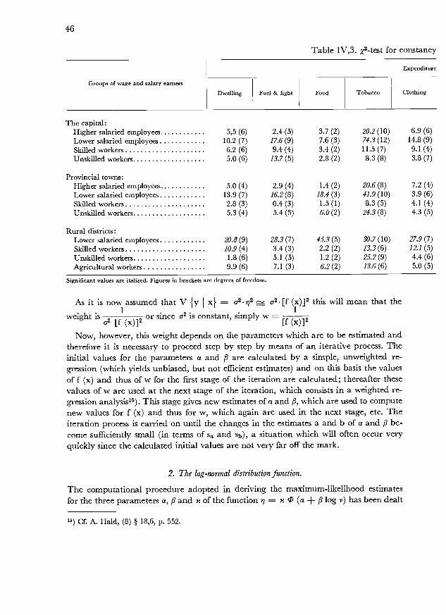
46

Significant values are italized. Figures in brackets are degrees of freedom.

As it is now assumed that V ' x = u2.rj2 i2. [f (x)]2 this will mean that the

weight is2 2

or since u2 is constant, simply w - 2u [f (x)] [f (x)]

Now, however, this weight depends on the parameters which are to be estimated andtherefore it is necessary to proceed step by step by means of an iterative process. Theinitial values for the parameters a and are calculated by a simple, unweighted re-gression (which yields unbiased, but not efficient estimates) and on this basis the valuesof f (x) and thus of w for the first stage of the iteration are calculated; thereafter thesevalues of w are used at the next stage of the iteration, which consists in a weighted re-gression analysis15). This stage gives new estimates of a and , which are used to computenew values for f (x) and thus for w, which again are used in the next stage, etc. Theiteration process is carried on until the changes in the estimates a and b of a and be-come sufficiently small (in terms of Sa and sb), a situation which will often occur veryquickly since the calculated initial values are not very far off the mark.

2. The log-normal distribution function.

The computational procedure adopted in deriving the maximum-likelihood estimatesfor the three parameters a, and x of the function s = (a + log r) has been dealt

15) Cf. A. Hald, (8) § 18,6, P. 552.

Table IV,3. X2-test for constancy

Groups of wage and salary earners

Expenditure

Dwelling Fuel & light Food Tobacco Clothing

The capital:Higher salaried employees 5,5 (6) 2.4 (5) 3.7 (2) 20.2(10) 6.9 (6)Lower salaried employees 10.2 (7) 17.6(9) 7.6 (3) 74.3 (12) 14.8 (9)Skilled workers 6.2 (6) 9.4 (4) 3.4 (2) 11.5 (7) 9.1 (4)Unskilled workers 5.0 (6) 13.7 (5) 2.8 (2) 8.3 (8) 3.8 (7)

Provincial towns:Higher salaried employees 5.0 (4) 2.9 (4) 1.4 (2) 20.6(8) 7.2 (4)Lower salaried employees 13.9 (7) 16.2(8) 18.4 (3) 41.9(10) 3.9 (6)Skilled workers 2.8 (3) 0.4 (3) 1.5 (1) 8.3 (5) 4.1 (4)Unskilled workers 5.3 (4) 5.4 (5) 6.0 (2) 24.3(8) 4.3 (5)

Rural districts:Lower salaried employees 20.8(9) 28.3(7) 45.3(5) 30.7(10) 27.9 (7)

Skilled workers 10.9 (4) 3.4 (3) 2.2 (2) 13.3(6) 12.1 (5)

Unskilled workers 1.8 (6) 5.1 (5) 1.2 (2) 25.2(9) 4.4 (6)Agricultural workers 9.9 (6) 7.1(3) 6.2 (2) 13.6(6) 5.0 (5)

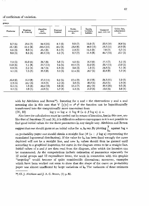
of coefficients of variation.

groups

1) Cf. J. Aitchison and J. A. C. Brown, (1) p. 82.

47

with by Aitchison and Brown16). Inserting for ii and r the observations y and x andassuming also in this case that V y[x = ci2 2 the function can be logarithmicallytransformed into the computionally more convenient form(IV, 10) log y = log + log 'P (a + log x) + g

Also here the calculations must be carried Out by means of iteration, but in this case, un-like that of functions (3) and (4), it is difficult to achieve convergence as it is not possible tofind good initial values for the three parameters in any simple way. Aitchison and Brown

suggest that one should guess at an initial value for ic, k0 say. By plotting against log x

on probability paper one should obtain a straight line ( (a + log x) representing thecumulated log-normal distribution). If the value for k0 has been fixed wrongly the curvedepicted will not be a straight line, and new k0 values should then be guessed untilaccording to a graphical inspection the curve in the diagram seems to be a straight line.Initial values of a and are then read from the diagram, after which the iteration canbe commenced. As the computations include estimation of parameters separately for12 social groups and 13 expenditure items, the work in connection with this graphic"targeting" would become of quite considerable dimensions; moreover, exampleswhich have been worked out seem to show that the shape of the curve on probabilitypaper was almost unaffected by large variations of ko The variances of these estimates

Footwear Washing& cleaning

Durablesexcl.

vehicles

Personalhygiene

Books,newspapers

etc.

Sports,holidays,hobbies

Transportincl, own car

Union fees,subscription

etc.

8.7(6) 23.6(7) 34.5(10) 8.7(6) 9.9(7) 10.9(7) 55.8(10) 14,4(6)18.1 (8) 15.2 (8) 100.0 (11) 14.2 (6) 23.0 (9) 44.9(11) 23.5(11) 20.9 (8)6.6 (5) 8.9 (4) 20.1(8) 8.4 (5) 2.3 (5) 12.5 (6) 7.8 (7) 0,7 (4)8.8 (5) 8.3 (6) 40.5(10) 4.2 (5) 8.7 (7) 11.3 (8) 40.7 (10) 15.7(5)

7.0 (5) 10.9 (6) 34.7(8) 5.8 (5) 4.0 (6) 16.5(6) 17.2(7) 5.2 (4)11.8(6) 7.1 (8) 52.7(11) 7.6(6) 10.5(7) 32.8(9) 53.7(11) 13.9(5)0.9 (3) 2.2 (4) 14.7 (5) 6.3 (3) 5.8 (5) 5.3 (5) 24.8 (5) 5.1(3)4.1 (4) 7.5 (5) 35.5(8) 5.0 (5) 12.4 (6) 24.7(6) 52.9(8) 5.7 (4)

16.0(6) 16.5(8) 57.5(11) 9.2 (6) 27.4(9) 37.5(9) 84.3(11) 7.9 (5)2.3 (4) 14.1 (5) 15.5(5) 4.2 (3) 5.9 (5) 30.3(6) 26.0 (5) 2.3 (3)6.1 (4) 1.9 (6) 44.0 (10) 3.8 (6) 12.5 (7) 48.2 (9) 59.3(10) 9.5 (3)4.1(4) 4.9 (5) 15.9(5) 4.7 (3) 4.5 (5) 21.9(6) 15.6(6) 3.6 (4)

48

of initial parameter values are thus very big and it was therefore deemed desirable towork out a method of estimation by which the initial values could be computed me-chanically.

As initial value for k war chosen ymax = the highest average value observed for y inthe groups of three households into which the basic material had been grouped.

Then initial values for a and were calculated by linear regression since (IV, 5)

implies that u = a + log x, where di (u) =

As a result of the method of calculation adopted the whole computation programmefor function (IV, 5) became "automatic". Naturally, there was no guarantee that theiteration would always converge; there was no possibility of ensuring in advance thatthe initial parameter estimates a0, b0 and k0 would fall within the region of conver-gence'7). It turned out in fact that in some cases (19 out of 156) the iteration processdiverged. As will be shown later in this chapter it also turned out that a fixed value ofthe parameter j3 had to be chosen to ensure workability of the estimation procedure.

All estimates of the parameters have been shown in appendix A; extracts of the resultsare shown and commented upon in chapter V.

IVe. Tests for Goodness of Fit.

Cf. J. Aitchison and J. A. C. Brown (1) p. 75.Cf. Durbin and Watson: (4).

1. The tests used.

One of the purposes of the present analysis was, as already mentioned, to find that oneof the chosen relations which according to the available observations would showforeach expenditure itemthe best goodness of fit. On the basis of such an investigationit would be possible to conclude that among the five given types of Engel curves, onetype gives the best fit if we consider the i'th expenditure item; in the case of the j'thexpenditure item it may be another function type which gives the best fit, and so on.To be able to draw such a conclusion one must test the goodness of fit of the five func-tions. These tests consist in various comparisons of the calculated function values, f (x),with the observed values of household expenditures y. The function which passes mostof these tests can then be said to give the best description of the relationship betweeny and i from the point of view of the available observations x and y.

In the present analysis the following tests have been used in evaluating the chosenfunctions:

Test for number of runs above and below the curve and test for length of run.Durbin and Watson's d-test'8).F-test for the ratio between the variance in the distribution of deviations from thecurve and the variance within groups,x2-test for normality of residuals.

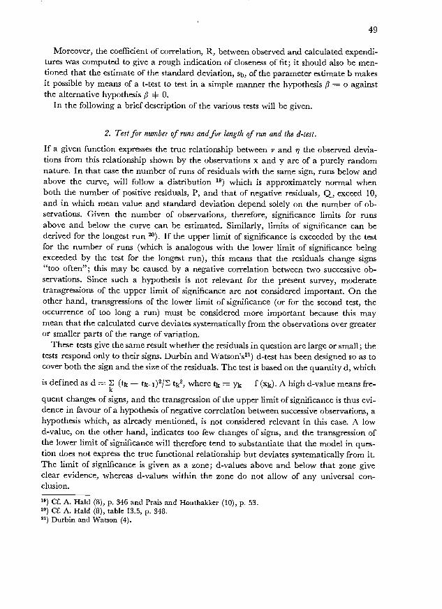
1) Cf. A. Hald (8), p. 346 and Prais and Houthakker (10), p. 53.2O) Cf. A. Hald (8), table 13.5, p. 348.21) Durbin and Watson (4).

49

Moreover, the coefficient of correlation, R, between observed and calculated expendi-tures was computed to give a rough indication of closeness of fit; it should also be men-tioned that the estimate of the standard deviation, sj, of the parameter estimate b makesit possible by means of a t-test to test in a simple manner the hypothesis = o againstthe alternative hypothesis fi 0.

In the following a brief description of the various tests will be given.

2. Test for number of runs and for length of run and the d-test.

If a given function expresses the true relationship between r and i the observed devia-tions from this relationship shown by the observations x and y are of a purely randomnature. In that case the number of runs of residuals with the same sign, runs below andabove the curve, will follow a distribution 19) which is approximately normal whenboth the number of positive residuals, P, and that of negative residuals, Q, exceed 10,and in which mean value and standard deviation depend solely on the number of ob-servations. Given the number of observations, therefore, significance limits for runsabove and below the curve can be estimated. Similarly, limits of significance can bederived for the longest run 20). If the upper limit of significance is exceeded by the testfor the number of runs (which is analogous with the lower limit of significance beingexceeded by the test for the longest run), this means that the residuals change signs"too often"; this may be caused by a negative correlation between two successive ob-servations. Since such a hypothesis is not relevant for the present survey, moderatetransgressions of the upper limit of significance are not considered important. On theother hand, transgressions of the lower limit of significance (or for the second test, theoccurrence of too long a run) must be considered more important because this maymean that the calculated curve deviates systematically from the observations over greateror smaller parts of the range of variation.

These tests give the same result whether the residuals in question are large or small; thetests respond only to their signs. Durbin and Watson's21) d-test has been designed so as tocover both the sign and the size of the residuals. The test is based on the quantity d, which

is defined as d = (tk - tk4)2/E tk2, where tk = yk - f (xk). A high d-value means fre-

quent changes of signs, and the transgression of the upper limit of significance is thus evi-dence in favour of a hypothesis of negative correlation between successive observations, ahypothesis which, as already mentioned, is not considered relevant in this case. A lowd-value, on the other hand, indicates too few changes of signs, and the transgression ofthe lower limit of significance will therefore tend to substantiate that the model in ques-tion does not express the true functional relationship but deviates systematically from it.The limit of significance is given as a zone; d-values above and below that zone giveclear evidence, whereas d-values within the zone do not allow of any universal con-clusion.

50

The tests for runs and the d-test will, of course, point in the same direction since theyaim at the same alternative hypothesis.

3. The F-test.

The F-test which compares the variance in the distribution of the residuals, y - f (x),y being the average in the groups of three observations, with the average variancewithin the groups, is suitable as a test of different alternative hypotheses although in thiscase, too, only one limit of significance (the upper one) is relevant.

The test hypothesis is here again that the chosen model = f (r) expresses the truerelationship between y and x and that the residuals, y - f (x), are everywhere distributedwith mean value O and variance ci2 = V yx . If the test hypothesis is correct, theestimate, s22, of the variance of the residuals will have the same true value as the estimate,

of the variance within groups, and the ratio between the two variances F = will

follow a F-distribution.

y

X

Figure IV, 3a. Type of systematic deviations which will berevealed by the run tests, and may be not by other tests.

y

X

Figure IV, 3b. Type of systematic deviations which will berevealed by the F-test, but may be not by the run tests.

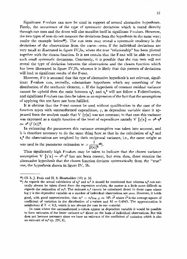
51

Significant F-values can now be cited in support of several alternative hypotheses.Firstly, the occurrence of the type of systematic deviations which is tested directlythrough run tests and the d-test will also manifest itself in significant F-values. However,the two types of tests do not measure the deviations from the hypothesis in the same way;confer the example below22). The run tests may reveal a systematic tendency in thedeviations of the observations from the curveeven if the individual deviations arevery small as illustrated in figure IV,3a, where the true "relationship" has been plottedtogether with the chosen function. It is not certain that the F-test will be able to revealsuch small systematic deviations. Conversely, it is possible that the run tests will notreveal the type of deviation between the observations and the chosen function whichhas been illustrated in figure IV,3b, whereas it is likely that this pattern of deviationswill lead to significant results of the F-test.

However, if it is assumed that this type of alternative hypothesis is not relevant, signif-icant F-values can, secondly, substantiate hypotheses which say something of thedistribution of the stochastic element, e. If the hypothesis of constant residual variancecannot be upheld then the ratio between s22, and s12 will not follow a F-distribution,and significant F-values can then be taken as an expression of the fact that the assumptionsof applying this test have not been fulfilled.

It is obvious that the F-test cannot be used without qualification in the case of thefunction types with untransformed expenditure, y, as dependent variable since it ap-peared from the analysis made that V yjx was not constant; in that case this variancewas expressed as a simple function of the level of expenditure namely V yx = a2

-' a2 [f (x)]2.In estimating the parameters this variance assumption was taken into account, and

it is therefore necessary to do the same thing here so that in the calculation of s22 andthe observations are weighted by their reciprocal variance, i.e., the same weight as

was used in the parameter estimation w 1 23).[f(x)]2

Thus significantly high F-values may be taken to indicate that the chosen varianceassumption V yjx = a2 n2 has not been correct, but even then, there remains thealternative hypothesis that the chosen function deviates systematically from the "true"one, the hypothesis shown in figure IV, 3b.

22) Cf. S. J. Prais and H. S. Houthakker (10) p. 52.52) As regards the actual calculation of and si2 it should be mentioned that whereas s can nat-

urally always be taken direct from the regression analysis, the matter is a little more difficult asregards the estimation of ai2. The estimate si2 cannot be calculated direct in those cases wherelog y is the dependent variable as a number of individual observations are zero. However, it holdsgood, with good approximation, that sj = 5i2(log ) M2. c2 where c2 is the average square ofcoefficient of variation in the distribution of y-values and M = 0.4343. The approximation issatisfactory if < 0.3, which is not always the case in our material.

In cases where the untransformed y-values appear as dependent variable it would be possibleto form estimates of the inner variance si2 direct on the basis of individual observations. But thisdoes not become necessary since we have an estimate of the coefficient of variation which is alsoan estimate of ai2 cp. (IV, 6).

52

4. The 2 -test.

To test the hypothesis that the residuals are normally distributed the f-test has beenused. The observed deviations are grouped, and by comparing this grouped distributionof deviations with a normal distribution with the same mean value (0) and variance isit possible to calculate a x2-quantity24). Also in this case it will, of course, be necessaryto insert the variance assumption used in the parameter estimation. Significantly highf-values support the alternative hypothesis that the deviations of the observations fromthe function are not normally distributed. Assuming that the tests referred to above havegiven insignificant results, it has, prior to the f-test, been possible to substantiate the fol-lowing hypothesis: The relationship suggested by the observations does not deviate system-atically from the proposed functional relationship (test for number of runs and size oflongest run, d-test and F-test), and the deviations of the observations from this functionhave everywhere a variance which is of the same magnitude as the variance withingroups (F-test). A significant f-value will then indicate that the residuals are not nor-mally distributed.

This alternative hypothesis can be further specified in the present case. For if it istrueas the test calculations seem to showthat the residuals are normally distributedin the case of the functions where the dependent variable is a logarithmic transformationof the expenditure, then the deviations from the function in the cases where the depen-dent variable is the untransformed value of expenditure will be log-normally distributed.And this is true even if one uses the weighted calculation method in the parameter estim-ation. Use of weights in the calculation influences the magnitude of the residuals, butnot the form of their distribution. One can thereforewith good support in the otherresults of the test calculationsadvance the assertion that significant f-values supportthe alternative hypothesis that the residuals are log-normally distributed25).

A comparison of the calculated values of the coefficient of correlation for the differentfunctions gives an impression of which of the five functions has the closest fit for eachexpenditure item in each group of wage and salary earners. However, such a directcomparison will only be possible if the residuals are at the same level, i.e., if the varianceassumption used in the parameter estimation, V yx = a2 [f (x)]2, is also used here asa basis for assigning weights. In the following chapter the results of this calculation aswell as of all the test calculations referred to above will be shown.

IV. f. Planning the Computation Programme and CarryingOut The Computations.

After specifying the five functional relationships and the procedure to be used in theirestimation the practical part of the analysis can be started. This part comprises work-ing out a detailed computation programme and the corresponding code for feeding it

Chapter V, p. 60.Chapter V, p. 64.

5. The coefficient of correlation.

i. e. DAnsk Sekvens Kalkulator.Cf. J. Aitchison and J. A. C. Brown (1) p. 82, and above p. 47.

53

into DASK26) and (at length) computation and printing of parameter estimates and theirstandard errors and of test resultsaccording to the tests referred to above.

It will be understood from what has been mentioned above that the computationprogramme is rather comprehensive. For each of the twelve groups of wage and salaryearners into which the basic material has been divided, parameter estimates and theirstandard errors are to be calculated separately for five Engel functions for a total of 13expenditure items. This gives a total of 12 x 5 x 13 = 780 sets of calculations; thesame number of tests have to be made. Coding the programme, therefore, was boundto require a great amount of work, and the fact that part of the computation programme(especially the part concerning the log-normal distribution and the regression analysiswith the above-mentioned special variance assumptions and some of the test calculations)had not previously been performed on the DASK rendered the coding even more difficult.

In planning the computation programme it was, of course, necessary to consider howthe individual operations were to be performed on the DASK, so that the computationprogramme could as far as possible be adapted to the capacity of that electronic com-puter. During the greater part of the analysis a very useful contact was established withthe division concerned at the Danish Institute of Computing Machinery.

In the present investigation it had been attempted to guard against "unforeseen"difficulties by working out in advance, at the consumer survey section of The StatisticalDepartement, examples of all the computing operations which were to be performedaccording to the computation programme.

In the course of this preliminary work several sources of error were traced, and severalcorrections had to be made in the computation programme and in the input tapebutnevertheless the performance of the computation programme on the DASK presentedseveral unpleasant surprises, two of which deserve to be mentioned because they seemto be of a certain theoretical interest.

The code for the computation programme was made so flexible that the compu-tation process could be stopped at all "vital" points and any necessary corrections bemade without re-running the whole programme. As a control measure which could beexpected to be very effective an inspection was introduced after all computations hadbeen run for the first of the twelve groups of wage and salary earners. Hereby it wasexpected that the weak spots which might have excaped the attention during the cal-culations of the examples mentioned above would be revealed.

This inspection of the results of the computations for the first group of wage and salaryearners showed that as regards function type (IV, 5) log ij = log x + log '2 (a + j log y)the computation programme did not work in five cases out of the thirteen expenditureitems comprised by the programme because the iterative process for the calculation of est-imates of x, a and did not converge27). This made essential changes in the programmenecessary, see below. For the other four functions the programme performance seemedfully satisfactory. Thanks to the flexibility of the code worked out for the computationprogramme the computations could be continued for these four functions, where the

54

results for the first group of wage and salary earners had been found satisfactory, whilethe corrections to the programme for the fifth function type were considered. But in thecourse of the continued run of the accepted programme for the four linear functionsit proved impossible in several cases as regards, functions (IV, 3) and (IV, 4), to obtainconvergence in the estimation of the parameters.

The reason for the lack of convergence in the case of function (IV, 5), must be foundin the fact that the variance V y Ix F in the distribution of the observed expenditurevalues is so big that the functional relationship between x and y can be satisfactorilydescribed by means of two parameters. Or in other words: With the given variancein the distribution of the observations one of the three parameters can be selectedarbitrarily within a wide interval, and the other two parameters can be estimatedconditioned by this arbitrarily selected parameter value without this causing any appre-ciable rise in the unexplained variance of y. The iterative procedure for determiningthe three parameter estimates becomes highly unstable, and in several cases convergencewill consequently not be obtained. And equally regrettable: in the cases where the itera-tion process did converge the standard deviations of the parameter estimates were sogreat that the estimates had to be considered almost useless, cf. table IV,4, whichshows the result of the computations for eight expenditure items in the group of higherpublic servants and salaried employees in the capital.

The table emphatically demonstrates that the results obtained are not very useful;the standard deviation of the estimates, apart from the food item, are of the same orderas the estimates themselves.

The "solution" chosen to this problem consisted in arbitrarily fixing in advance aconvenient value of the parameter , namely unity; it should be added that unity doesnot significantly deviate from any of the calculated j3-values in the three-parametercalculation, cf. table IV,4. This solution was also chosen by Aitchison and Brownin their analysis of British household budgets28). However, it does not appear from theirreport whether they had previously experienced just as disappointing results in thethree parameter estimation as was the case in the present analysis.

The reason for the cases of lacking convergence which occurred in the iterative cal-culation of parameter estimates in functions

(IV,3) = a--(logvlogv)and

(IV, 4)

was to be found in an unfortunate property of the estimation procedure adopted. Asmentioned above, p. 44, it was found that it applied to the functions in which the un-transformed value y was the dependent variable that V yx

F= a2 2 for which reason

it was decided to carry through the regression analysis with2

as weights; the test[f(x)]

calculations were carried through in accordance with the same principle in ordei to

) Cf. J. Aitchison and J. A. C. Brown (1) p. 130.

Table IV,4. Parameter estimates in the three-parameter case of the function

55

obtain everywhere as efficient estimators as practically possible. If, however f (x) assumesvery low values, in the extreme case zero, the weight factor for the value or values inquestion will completely dominate the calculation, and the iteration process, which wasmentioned on p. 46, will become quite unstable. If the initial parameter estimates orone of the subsequent estimates in the iteration process results in such low values off (x), there will be a risk that the iteration will stop. The reason why the group of wageand salary earners which was computed first, viz, higher public servants and salariedemployees, passed through without any stop as the only one of all the groups, is thatthe x-values in this group are rather large so that no f (x) values came close to zero.

The correction which was made in the computation programme to enable calculationsof parameter estimates to be made in the 41 cases (out of a total of 143) in the other 11groups of wage and salary earners in which the iteration process did not converge con-sisted in rejecting the special variance assumption and estimating on the assumptionof constant variance, i.e. applying the estimation procedure from the function types inwhich the logarithmically transformed expenditure, log y, is the dependent variable.The parameter values and test values thus estimated are not efficient, but this estimationprocedure were preferred rather than rejecting observations or omitting estimation29).

29) As mentioned p. 40, Prais and Houthakker, in their analysis, have everywhere used this estimationprocedure.

log = log x + log [ (a + log r)]. Higher public servants and salaried employeesin the Capital.

Expenditure item k 'k a 'a b Sb

Dwelling convergence not obtainedFuel and light 7600 63000 4.796 1.1 0.793 1.4Food 2900 950 6.192 2.0 1.62 0.64Tobacco 6700 820 7.517 5.3 1.87 1.7Clothing 3200 5600 6.431 2.6 1.44 1.0Foot wear 230 220 5.084 4.8 1.34 1.6Washing and cleaning 380 320 7.414 3.3 1.84 1.1Durables convergence not obtainedPersonal hygiene 1500 4800 5.460 2.2 1.10 1.1

Books, newspapers etc. convergence not obtainedSports, holidays, hobbies 13000 30000 7.834 2.3 1.63 0.93Transport (incl, own car) convergence not obtainedUnion fees, subscriptions etc. 660 2100 4.861 3.0 1.03 1.4

Chapter V.

MAIN RESULTS.

Va. Introductory remarks.

In this chapter some of the main results of the Engel curve analysis will be discussed.In the next chapter some results of certain further calculations will be put forward,but as already mentioned the main object of this inquiry has been the Engel curveanalysis.

In the appendix is shown, separately for each of the twelve groups of wage and salaryearners, parameter estimates and test results for five Engel functions (1,1) to (1,5) of thethirteen expenditure items.

However, it may perhaps be natural to try to boil down the somewhat overwhelmingabundance of figures in these tables.1) How can the result of the analysis be summed up?

In doing so the point of departure will be taken in the description of the object ofthe analysis which was given in chapter IV, p. 31, where the object was characterizedby the following two steps:

I) calculation of parameter estimates in the selected models and2) testing these models by various tests for goodness of fit.It will first be examined whether the tests for goodness of fit point in the same direction

or, in other words, whether it is possible to classify the selected Engel functions on thisbasis. Then follows an interpretation of the calculated parameter values.

The following tests were used (cf. p. 48 above):The coefficient of correlation between calculated and observed values (no proper

test, but the size of the coefficient of correlation can be taken as a measure of the"closeness of fit" of the relations proposed.2)

Test for number of runs.Test for longest run (where a run is defined as a series of positive or negative de-

viations between calculated and observed values).The d-test, in which both the signs and the numerical values of the deviations enter.The F-test, the ratio of the variance within groups and the variance of the residuals.The x2-test for the normality of the distribution of the residuals.

The proper tests fall into three categories. 10. The x2-test is concerned with the formof the distribution of the deviations between the calculated and the observed values,the test hypothesis being that these deviations are normally distributed. 2°. The variance-

More specifically 5 (models) x 12 (groups of wage and salary earners) X 13 (expenditure items) =780 less 19 cases in which the estimation procedure failed (model (1,5)) = 761 sets of parameterestimates and corresponding test results.Cf. Prais & Houthakker, (10), p. 95.

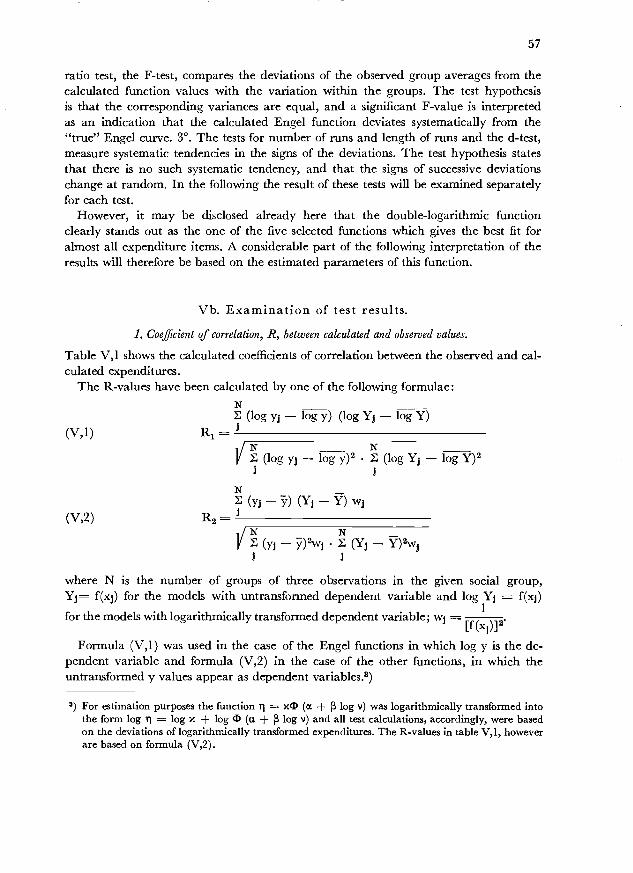
N

V (logy1 logy)2. (logY1 - logY)2i I

N(y - ) (Y - Y) wj

(V,2) R2IN N(yj - w1 (Y1 - Y)2w1

where N is the number of groups of three observations in the given social group,Y1= f(xj) for the models with untransformed dependent variable and log Yj = f(xj)

for the models with logarithmically transformed dependent variable; wj= [f( )]2

Formula (V, 1) was used in the case of the Engel functions in which log y is the de-pendent variable and formula (V,2) in the case of the other functions, in which theuntransformed y values appear as dependent variables.3)

57

ratio test, the F-test, compares the deviations of the observed group averages from thecalculated function values with the variation within the groups. The test hypothesisis that the corresponding variances are equal, and a significant F-value is interpretedas an indication that the calculated Engel function deviates systematically from the"true" Engel curve. 3°. The tests for number of runs and length of runs and the d-test,measure systematic tendencies in the signs of the deviations. The test hypothesis statesthat there is no such systematic tendency, and that the signs of successive deviationschange at random. In the following the result of these tests will be examined separatelyfor each test.

However, it may be disclosed already here that the double-logarithmic functionclearly stands out as the one of the five selected functions which gives the best fit foralmost all expenditure items. A considerable part of the following interpretation of theresults will therefore be based on the estimated parameters of this function.

Vb. Examination of test results.

1. Coefficient of correlation, R, between calculated and observed values.

Table V, i shows the calculated coefficients of correlation between the observed and cal-culated expenditures.

The R-values have been calculated by one of the following formulae:N

(log y - log y) (log Y1 - log Y)(V,l) R1=1

8) For estimation purposes the function t = xD (c + 3 log y) was logarithmically transformed intothe form log i log x + log I (a + 3 log y) and all test calculations, accordingly, were basedon the deviations of logarithmically transformed expenditures. The R-values in table V, 1, howeverare based on formula (V,2).

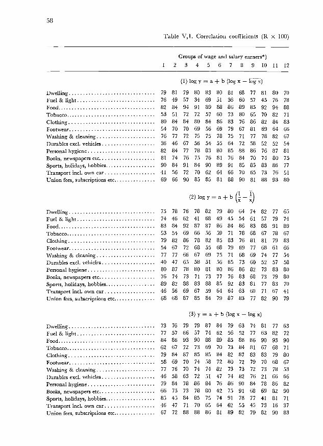
58

Table V,l. Correlation coefficients (R X 100)

1 2

Groups of wage and salary earners*)

3 4 5 6 7 8 9 10 il 12

(l)logy=a+b(logxlogx)Dwelling 79 81 79 80 83 80 81 68 77 81 80 70

Fuel & light 76 49 57 34 69 51 36 60 57 45 76 78

Food 82 84 94 91 89 88 86 89 85 92 94 88Tobacco 53 51 72 72 57 60 73 80 65 70 82 71

Clothing 80 84 84 80 84 86 83 76 86 82 84 83Footwear 54 70 70 69 56 69 79 67 81 69 64 66

Washing & cleaning 76 77 72 75 75 78 75 71 77 78 82 67

Durables excl, vehicles 36 46 67 56 54 55 64 72 58 52 52 54Personal hygiene 82 84 77 78 83 80 85 88 86 76 87 81

Books, newspapers etc. 81 74 76 75 76 81 76 84 70 74 80 75

Sports, holidays, hobbies 90 84 91 84 90 89 91 85 85 83 86 77Transport incl, own car 41 56 72 70 62 64 66 70 65 73 76 51

Union fees, subscriptions etc 69 66 90 85 85 81 88 90 81 88 93 80

(2)logy=a+b (!_)

Dwelling 75 78 76 78 82 79 80 64 74 82 77 65

Fuel & light 74 46 62 41 68 49 45 54 61 57 79 74

Food 83 84 92 87 87 86 84 86 83 88 91 89Tobacco 53 54 69 66 56 59 71 78 68 67 78 67

Clothing 79 82 86 78 82 85 83 76 81 81 79 83

Footwear 54 67 72 68 55 68 79 69 77 68 61 66Washing & cleaning 77 77 66 67 69 75 71 68 69 74 77 54Durables excl, vehicles 40 47 65 58 51 56 65 73 60 52 57 58

Personal hygiene 80 87 78 80 01 80 86 86 82 73 83 80

Books, newspapers etc 76 74 73 71 73 77 76 83 68 73 79 80Sports, holidays, hobbies 89 82 88 83 88 85 92 83 81 77 83 70

Transport incl, own car 46 56 69 67 59 64 64 63 60 71 67 41

Union fees, subscriptions etc 68 68 87 85 84 79 87 83 77 82 90 79

(3) y = a + b (log x - i- ;)

Dwelling 73 76 79 79 87 84 79 63 74 81 77 63

Fuel & light 77 57 66 57 74 62 56 52 77 63 82 72

Food 84 86 93 90 88 89 85 88 86 90 93 90

Tobacco 62 67 72 73 69 70 73 84 81 67 68 71

Clothing 79 84 87 85 85 84 82 87 83 83 79 80

Footwear 58 69 70 74 58 72 80 72 79 70 68 67

Washing & cleaning 77 76 70 74 74 82 73 73 72 73 78 53

Durables excl, vehicles 46 58 63 72 51 47 74 82 76 21 66 66

Personal hygiene 79 84 78 86 84 76 86 90 84 78 86 82

Books, newspapers etc. 66 75 73 78 80 42 75 91 68 69 82 90Sports, holidays, hobbies 85 45 84 85 75 74 91 78 77 41 81 71

Transport incl, own car 46 47 71 70 65 64 62 55 45 73 16 37

Union fees, subscriptions etc. 67 72 88 88 86 81 89 82 79 82 90 83

between observed and calculated expenditures.

59

Groups of wage and salary earners*)

1 2 3 4 5 6 7 8 9 10 11 12

Il l\-Dwelling 70 67 76 78 85 81 73 50 66 79 67 64Fuel & light 73 53 69 53 69 56 60 42 73 66 80 71Food 81 83 89 84 79 83 80 79 79 84 87 87Tobacco 62 72 67 60 63 67 69 78 74 64 73 66Clothing 74 68 84 83 80 80 78 86 76 77 69 72Footwear 57 66 73 75 60 72 78 79 71 71 66 64Washing & cleaning 75 72 65 67 70 76 69 71 66 65 73 46Durables excl, vehicles 47 62 60 71 48 52 73 77 76 42 68 66Personal hygiene 75 78 79 88 79 73 85 84 79 73 80 76Books, newspapers etc 56 70 68 70 76 41 73 85 67 66 75 88Sports, holidays, hobbies 79 69 77 81 69 65 84 71 74 50 52 64Transport incl, own car 54 42 67 66 60 58 24 52 46 65 45 29Union fees, subscriptions etc 63 67 81 86 83 74 84 78 86 72 88 78

(5) log y log k + log D (a + log x)

Dwelling 72 78 78 79 83 81 80 65 76 27 75 59Fuel & light 76 56 64 55 73 62 53 53 74 59 80 71Food 84 85 94 - 88 89 85 89 86 - 94 90Tobacco 62 65 72 - 68 68 70 79 76 66 47 70Clothing 79 - 84 82 - 84 82 76 61 - 82 82Footwear 58 69 69 73 58 71 79 68 81 68 68 67Washing & cleaning 77 76 71 76 72 79 71 69 73 76 79 52Durables excl, vehicles 43 50 66 68 48 46 - 74 58 59 59 60Personal hygiene 79 83 76 81 82 76 84 88 86 78 86 83Books, newspapers etc. 70 75 73 79 72 79 74 - 71 21 82 84Sports, holidays, hobbies 64 55 67 - - 65 89 - - 56 58 -Transport incl, own car 34 43 42 66 55 - - - 30 - - 34Union fees, subscriptions etc 67 72 49 61 84 82 89 62 80 86 - 82

(4) y = a + b

*) 1, Higher public servants and salaried employees. The capital. 2. Lower public servants and salaried employees.The capital. 3. Skilled workers. The capital. 4. Unskilled workers, The capital. 5. Higher public servants andsalaried employees. Provincial towns. 6. Lower public servants and salaried employees. Provincial towns. 7. Skilledworkers. Provincial towns. 8. Unskilled workers. Provincial towns. 9. Lower public servants and salaried employees.Rural districts. 10. Skilled workers. Rural districts. 11. Unskilled workers. Rural districts. 12. Agriculturalworkers. Rural districts.

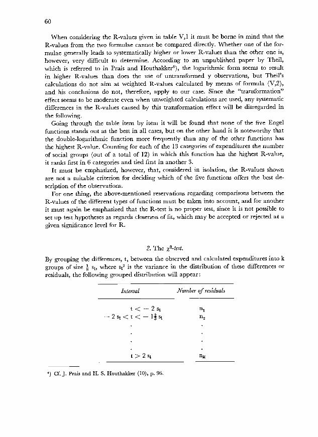
60

When considering the R-values given in table V, i it must be borne in mind that theR-values from the two formulae cannot be compared directly. Whether one of the for-mulae generally leads to systematically higher or lower R-values than the other one is,however, very difficult to determine. According to an unpublished paper by Theil,which is referred to in Prais and Houthakker4), the logarithmic form seems to resultin higher R-values than does the use of untransformed y observations, but Thejl'scalculations do not aim at weighted R-values calculated by means of formula (V,2),and his conclusions do not, therefore, apply to our case. Since the "transformation"effect seems to be moderate even when unweighted calculations are used, any systematicdifferences in the R-values caused by this transformation effect will be disregarded inthe following.

Going through the table item by item it will be found that none of the five Engelfunctions stands out as the best in all cases, but on the other hand it is noteworthy thatthe double-logarithmic function more frequently than any of the other functions hasthe highest R-value. Counting for each of the 13 categories of expenditures the numberof social groups (Out of a total of 12) in which this function has the highest R-value,it ranks first in 6 categories and tied first in another 3.

It must be emphasized, however, that, considered in isolation, the R-values shownare not a suitable criterion for deciding which of the five functions offers the best de-scription of the observations.

For one thing, the above-mentioned reservations regarding comparisons between theR-values of the different types of functions must be taken into account, and for anotherit must again be emphasized that the R-test is no proper test, since it is not possible toset up test hypotheses as regards closeness of fit, which may be accepted or rejected at agiven significance level for R.

2. The 2 -test.

By grouping the differences, t, between the observed and calculated expenditures into kgroups of size s, where st2 is the variance in the distribution of these differences orresiduals, the following grouped distribution will appear:

4) Cf. J. Prais and H. S. Houthakker (10), p. 96.

Interval Number of residuals

t < - 2 St n'- 2 St < t < - lIst n2

t>2st

61

This distribution is then compared with a similarly grouped, normal distribution withthe same mean and variance and with the same number of elements as the empirical

distribution, L = n3.

For each group in the distribution of the residuals is calculated the difference(nj - L 1) between number of elements in the empirical and in the theoretical, normaldistribution, e3 denoting the expected frequency in the j'the group. The quantity

(n - Lej)2/Lej

will then be approximately 2-distributed with k-m-1 degrees of freedom if the testhypotesis concerning the normality of the residuals is correct; m is the number of para-meters in the given Engel function, and k is the number of groups after it has been ensured,through a suitable merging of too small groups, that everywhere

L ej> 5

The 2-values have been shown in table V,2.It holds good for all expenditure items, with the exception of the expenditure on tobacco,

that the functions in which log y is the dependent variable, show the fewest significantx2-values.

In the case of several expenditure items there is only one social group out of twelvewhich has significant 2-values for these two functions.

It thus seems evident that this test points to one of the logarithmically transformedEngel functions as being the bestwhich of them must be left open until further evidencecan be put forward as they do almost equally well.

In the case of the types of function in which the untransformed value, y, appears asthe dependent variable it does not seem possible, however, to accept the hypothesisthat t is normally distributed. It has been taken into account, in connection with theparameter estimation and subsequent tests for these two functions, that the varianceof y (for given x) increases with the value of y. According to the investigations madethis relationship could be described with good approximation by the formula

V y x = 2 [f(x)]2 s2 [f(x)]2

wherefore the tests have been based on the quantity:

f(x) - yf(x)

Hereby was obtained that the variance in the distribution of t could be consideredconstant and independent of x. On the other hand, as the x2-tests show, the distributionsobtained are evidently not normal.

It will be found, however, that the results achieved correspond closely to what wasto be expected from the discussion on this subject in chapter IV, p. 52. It was concluded

62

Table V,2.

1 2 3 4

Groups of wage and salary earners*)5 6 7 8 9 10 11 12

(l)logy=a+b(logx-logx)Dwelling 9.9 5.2 4.5 4.1 5.4 9.4 7.0 4.6 5.0 0.6 3.8 6.6Fuel & light 6.3 25.5 10.8 8.0 3.8 15.0 6.5 3.1 23.4 2.3 17.7 8.6Food 8.9 10.2 1.4 8.5 7.1 5.8 3.9 2.8 2.8 9.4 9.0 5.8Tobacco 21.5 30.4 6.1 14.6 9.0 32.0 5.8 4.9 11.1 5.9 11.7 1.6Clothing 8.4 8.5 8.7 13.3 6.4 6.1 2.1 6.3 5.5 3.0 3.6 3.2Footwear 10.0 9.4 9.8 7.3 5.0 10.9 2.8 1.6 6.7 8.6 8.9 2.4Washing & cleaning 12.4 13.8 5.0 9.0 3.8 5.6 0.7 7.8 3.7 1.1 9.0 8.8Durables excl, vehicles 3.9 8.2 12.8 9.7 14.6 12.6 2.2 3.2 6.8 3.7 7.3 1.3Personal hygiene 5.1 9.1 6.6 5.0 6.8 7.0 3.7 7.0 14.9 11.5 3.8 5.6Books, newspapers etc 10.6 9.9 0.9 3.4 7.4 12.6 4.3 2.8 8.3 1.5 5.2 6.1Sports, holidays, hobbies. . 6.0 3.9 4.5 3.3 10.2 8.5 5.0 14.0 4.6 7.1 5.2 1.8Transport incl, own car. . 25.7 40.3 3.8 5.1 6.7 7.1 0.5 4.6 5.7 4.9 4.0 9.7Union fees, subscriptions etc. 3.3 10.2 5.0 8.0 4.1 6.4 13.0 4.9 8.1 6.6 10.6 3.595% significance level 14.1 16.9 11.1 14.1 11.1 14.1 7.8 11.1 14.1 7.8 14.1 7.8Degrees of freedom 7 9 5 7 5 7 3 5 7 3 7 3

(I i(2) log y = a + b x

Dwelling 5.9 4.8 3.3 9.9 4.6 3.9 5.3 3.2 7.7 4.1 7.4 2.6Fuel & light 7.4 16.7 4.5 13.7 6.0 9.6 9.6 3.2 20.7 2.9 8.2 4.7Food 8.8 10.9 0.9 7.3 14.0 4.3 0.9 1.8 2.4 2.2 2.9 1.8Tobacco 12.9 38.8 1.1 14.6 10.6 18.9 6.4 9.7 13.4 3.7 10.6 0.6Clothing 9.2 3.2 6.6 19.7 5.4 7.7 3.2 9.4 4.5 6.2 1.5 6.3Footwear 6.5 5.8 3.6 7.0 3.0 15.5 5.4 1.9 9.0 3.7 11.7 2.9Washing & cleaning 8.6 7.8 5.0 9.8 13.5 5.8 1.2 1.4 3.5 3.2 10.5 1.7Durables excl, vehicles 11.5 9.1 5.5 15.0 10.6 17.6 0.1 3.0 2.9 2.6 7.8 1.1Personal hygiene 6.6 7.0 8.4 8.8 4.5 10.4 2.7 2.9 6.2 10.6 14.1 5.3Books, newspapers etc 11.6 6.7 3.0 9.0 6.7 15.2 4.1 3.3 8.1 1.3 8.8 3.3Sports, holidays, hobbies. . . 4.6 5.0 4.0 2.2 3.0 2.5 0.4 4.2 6.7 2.3 4.9 6.6Transport incl, own car 16.9 34.0 5.1 7.6 11.8 8.7 1.2 3.4 5.5 2.0 4.5 8.1Union fees, subscriptions etc. 6.9 8.2 4.2 10.2 11.9 7.0 7.8 3.1 10.8 2.2 9.4 3.495% significance level 14.1 16.9 11.1 14.1 11.1 14.1 7.8 11.1 14.1 7.8 14.1 7.8Degrees of freedom 7 9 5 7 5 7 3 5 7 3 7 3

(3) y = a + b (log x - log x)Dwelling 17.2 18.9 2.7 12.9 12.6 13.5 2.5 12.9 9.5 5.4 11.3 4.9Fuel & light 14.8 22.0 8.0 8.8 3.6 3.8 6.9 12.0 8.1 3.3 17.7 20.2Food 13.1 10.7 7.1 3.5 12.5 4.0 1.4 1.5 8.9 3.4 5.9 0.8Tobacco 3.6 11.6 6.9 10.7 6.5 6.0 6.9 3.8 12.5 5.4 - 3.2Clothing 4.3 13.2 2.4 9.0 7.1 11.9 2.6 9.0 19.4 0.5 15.2 2.1Footwear 8.6 13.8 18.9 2.2 3.1 21.5 2.7 4.7 13.9 4.0 5.1 8.5Washing & cleaning 10.4 25.1 13.5 14.7 8.0 14.3 1.3 11.1 14.0 7.0 31.4 3.2Durables excl. vehicles 39.6 60.0 3.9 5.4 31.9 91.1 9.3 10.4 38.8 - 26.2 2.7Personal hygiene 17.7 36.9 1.8 13.9 13.8 36.9 4.8 7.9 18.6 4.5 27.4 3.6

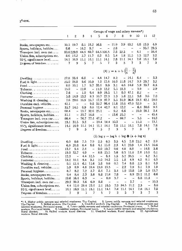
Z2-test.

63

*) 1. Higher public servants and salaried employees. The Capital. 2. Lower public servants and salaried employees.The Capital. 3. Skilled workers. The Capital. 4. Unskilled workers. The Capital. 5. Higher public servants andsalaried employees. Provincial towns. 6. Lower public servants and salaried employees. Provincial towns. 7. Skilledworkers. Provincial towns. 8. Unskilled workers. Provincial towns. 9. Lower public servants and salaried employees.Rural districts. 10. Skilled workers. Rural districts. 11. Unskilled workers. Rural districts. 12. Agriculturalworkers. Rural districts.

1 2 3

Groups of wage and salary earners*)4 5 6 7 8 9 10 11 12

Books, newspapers etc 50.5 19.7 8.1 18.2 16.8 - 11.0 3.9 43.2 4.8 13.9 4.0Sports, holidays, hobbies. . . 8.6 - 14.2 9.7 - - 2.8 - - - 35.7 29.5Transport incl. own car 80.6 229.8 44.3 60.7 64.5 100.5 7.8 52.5 - 4.1 - 34.4Union fees, subscriptions etc. 8.6 14.2 2.7 11.7 8.3 8.5 5.4 1.8 11.5 1.5 12.7 3.295% significance level 14.1 16.9 11.1 14.1 11.1 14.1 7.8 11.1 14.1 7.8 14.1 7.8

Degrees of freedom 7 9 5 7 5 7 3 5 7 3 7 3

(4) y = a + b (!_ I)

Dwelling 27.8 33.4 6.8 - 4.8 14.7 8.2 - 14.1 8.4 - 3.3Fuel & light 25.0 34.8 9.6 10.9 1.2 12.4 10.3 11.8 14.7 3.3 20.7 3.2Food 8.0 10.1 1.7 9.7 33.4 9.0 3.1 4.6 14.8 5.9 33.7 8.3Tobacco 15.0 - 12.8 - 11.9 12.2 5.5 18.3 - 3.9 - 2.9Clothing 7.6 - 1.0 9.4 9.9 19.5 1.1 8.0 47.1 8.2 - -Footwear 5.8 14.9 13.3 8.3 10.7 27.3 1.3 5.8 22.1 3.8 3.6 7.0Washing & cleaning 7.6 29.6 16.9 16.7 17.9 37.7 5.5 31.9 36.8 19.3 42.1 10.0

Durables excl, vehicles 42.1 - - 9.8 32.7 98.4 11.8 19.6 47.0 52.0 - 5.1

Personal hygiene 35.7 54.5 6.9 8.6 12.4 42.7 8.1 12.2 - 6.4 30.6 9.3Books, newspapers etc 68.4 - 13.7 32.6 25.1 - 9.2 6.6 - 10.0 28.1 2.4Sports, holidays, hobbies. . . 35.1 - 20.7 16.8 - - 13.6 25.2 - - - 45.4Transport incl, own car. 86.4 - 56.7 77.4 47.2 - - 88.7 - 5.5 - 44.3Union fees, subscriptions etc. 23.1 31.5 3.3 - 23.4 18.4 10.3 - -. 11.0 - 13.195% significance level 14.1 16.9 11.1 14.1 11.1 14.1 7.8 11.1 14.1 7.8 14.1 7.8

Degrees of freedom 7 9 5 7 5 7 3 5 7 3 7 3

(5) log y = log k + log C1 (a + log x)

Dwelling 6.0 6.6 7.5 7.9 2.5 6.5 3.5 4.5 2.8 25.2 4.2 2.9Fuel & light 6.3 20.8 8.4 8.8 4.1 15.0 2.3 4.1 20.9 1.4 14.5 10.6Food 13.7 9.4 2.4 - 9.0 10.7 0.6 4.8 8.9 - 14.8 3.6Tobacco 19.0 32.7 4.9 - 8.8 25.5 5.6 8.5 11.0 2.8 14.0 0.1

Clothing 12.3 - 4.4 12.5 8.4 1.5 5.2 34.5 - 4.2 3.1

Footwear 13.2 10.1 9.4 9.1 2.0 14.2 5.5 1.8 4.9 4.2 9.1 4.0Washing & cleaning 9.1 12.4 6.1 11.6 5.8 9.6 0.5 7.4 8.8 2.5 8.1 4.9Durables excl, vehicles 5.9 8.9 4.8 10.4 13.0 13.5 - 2.2 7.9 3.1 7.9 1.9

Personal hygiene 8.7 8.2 7.2 2.7 8.4 7.1 3.4 1.9 13.8 5.9 5.0 13.7

Books, newspapers etc 9.4 8.4 2.3 3.6 9.8 11.8 7.8 - 8.9 23.2 11.2 6.6Sports, holidays, hobbies. . . 19.6 16.4 6.3 - - 8.0 3.7 - - 8.8 11.3

Transport incl, own car 29.3 39.3 3.6 6.0 8.8 - - - 3.7 - - 10.3Union fees, subscriptions etc. 4.4 12.0 29.4 23.4 2.1 10.5 7.9 34.5 11.2 2.3 - 3.095% significance level 14.1 16.9 11.1 14.1 11.1 14.1 7.8 11.1 14.1 7.8 14.1 7.8Degrees of freedom 7 9 5 7 5 7 3 5 7 3 7 3

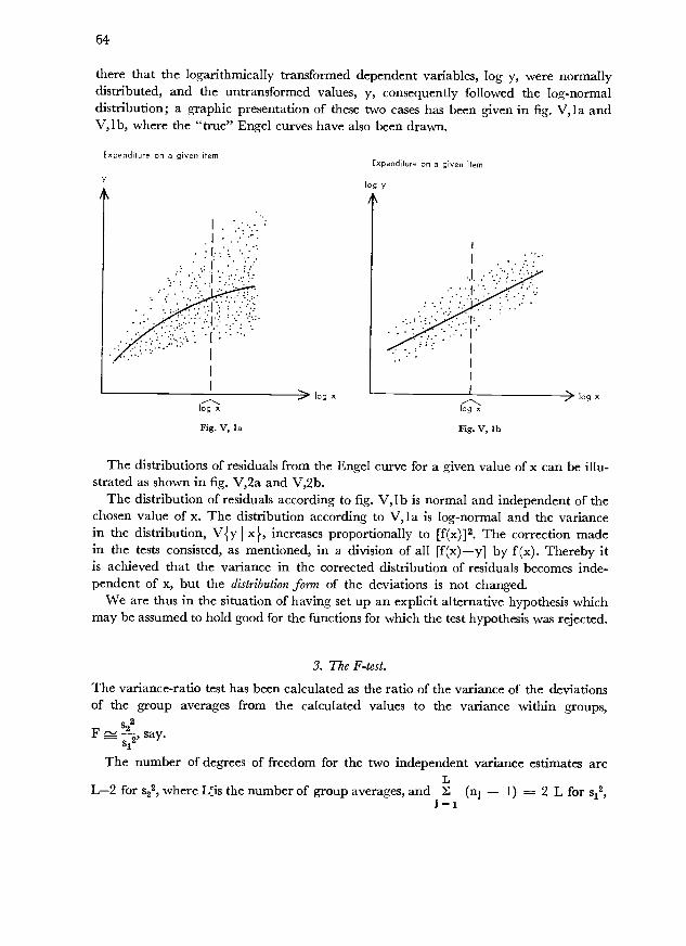
64

there that the logarithmically transformed dependent variables, log y, were normallydistributed, and the untransformed values, y, consequently followed the log-normaldistribution; a graphic presentation of these two cases has been given in fig. V,la andV, lb, where the "true" Engel curves have also been drawn.

Expenditure on a given Item

y

log x

Expenditure on a given item

log y

log x

Fig. V, lb

log x

The distributions of residuals from the Engel curve for a given value of x can be illu-strated as shown in fig. V,2a and V,2b.

The distribution of residuals according to fig. V, lb is normal and independent of thechosen value of x. The distribution according to V, I a is log-normal and the variancein the distribution, V y x , increases proportionally to [f(x)]2. The correction madein the tests consisted, as mentioned, in a division of all {f(x) _y] by f(x). Thereby itis achieved that the variance in the corrected distribution of residuals becomes inde-pendent of x, but the distribution form of the deviations is not changed.

We are thus in the situation of having set up an explicit alternative hypothesis whichmay be assumed to hold good for the functions for which the test hypothesis was rejected.

3. The F-test.

The variance-ratio test has been calculated as the ratio of the variance of the deviationsof the group averages from the calculated values to the variance within groups,

F 2' say.

The number of degrees of freedom for the two independent variance estimates areL

L-2 for s22, where Lis the number of group averages, and E (nj - I) = 2 L for s12,J 1

yFig. V, 2a Frequency of expenditure for given income

og yFig. V, 2b Frequency of log expenditure for given income

y

log y

65

66

Table V,3. F-test for linearity (ratio between

1 2 3

Groups of wage and salary earners*)4 5 6 7 8 9 10 11 12

(1) log y = a + b (log x - log x)

Dwelling 1.45 1.24 1.05 1.14 0.73 1.09 0.83 1.38 0.92 0.95 1.31 1.31

Fuel & light 1.30 1.31 0.78 1.92 0.96 1.00 1.21 1.12 1.25 1.30 1.04 1.36

Food 1.59 1.19 0.67 1.02 0.78 1.20 1.67 0.83 1.12 1.17 0.85 1.21

Tobacco 1.57 1.43 1.27 1.32 1.45 1.56 1.07 0.86 1.60 0.81 1.22 1.56

Clothing 1.20 1.14 1.23 1.06 1.07 1.10 1.25 1.84 0.95 0.99 1.47 1.54

Footwear 1.19 0.99 0.96 0.92 1.34 1.10 0.79 1.46 0.79 0.89 1.25 0.87Washing & cleaning 1.10 1.02 1.27 1.11 1.29 1.22 1.52 1.21 1.08 0.99 0.91 2.07Durables excl, vehicles 2.16 1.89 1.76 1.80 2.10 1.97 2.88 1.33 1.85 2.41 1.75 1.39

Personal hygiene 1.05 1.37 1.25 1.30 0.89 1.47 0.68 1.01 0.94 1.48 0.94 0.94Books, newspapers etc. 0.97 1.46 0.91 1.39 1.48 1.14 1.04 0.90 1.37 1.20 0.96 1.54Sports, holidays, hobbies 0.91 1.20 0.86 1.14 0.95 1.28 0.87 1.20 1.55 1.51 1.23 1.54

Transport incl, own car 2.84 2.50 2.04 1.36 2.97 2.24 1.92 1.85 2.05 1.91 1.54 2.20Union fees, subscriptions etc.. . 1.17 1.29 0.77 1.28 0.95 1.50 0.66 0.91 1.38 1.05 0.79 1.27

95% significance level 1.31 1.26 1.36 1.41 1.40 1.31 1.48 1.40 1.32 1.48 1.34 1.47

f1 110 152 81 66 68 109 49 68 100 49 91 51

f0 224 308 166 136 140 222 102 140 204 102 186 106

(2) logy = a + b ( - I)

Dwelling 1.69 1.43 1.16 1.21 0.76 1.15 0.89 1.55 1.02 0.91 1.51 1.47

Fuel & light 1.37 1.36 0.70 1.81 0.99 1.04 1.10 1.25 1.18 1.11 0.93 1.58

Food 1.53 1.18 0.87 1.48 0.93 1.40 1.86 1.03 1.22 1.66 1.20 1.17Tobacco 1.56 1.38 1.38 1.54 1.48 1.60 1.15 0.94 1.51 0.87 1.43 1.74

Clothing 1.26 1.26 1.14 1.13 1.16 1.23 1.29 1.82 1.32 1.05 1.85 1.55

Footwear 1.19 1.07 0.90 0.96 1.36 1.13 0.82 1.42 0.95 0.92 1.33 0.88Washing & cleaning 1.09 1.04 1.47 1.38 1.53 1.38 1.71 1.29 1.38 1.13 1.13 2.65Durables excl, vehicles 2.08 1.88 1.86 1.73 2.19 1.92 2.78 1.30 1.80 2.38 1.61 1.31

Personal hygiene 1.14 1.37 1.18 1.22 1.00 1.49 0.63 1.10 1.18 1.64 1.20 0.95Books, newspapers etc. 1.21 1.45 1.01 1.59 1.65 1.39 1.03 0.95 1.47 1.21 1.01 1.25

Sports, holidays, hobbies 0.98 1.35 1.16 1.21 1.09 1.63 0.85 1.34 1.92 1.99 1.53 1.91

Transport incl, own car 2.70 2.50 2.20 1.47 3.15 2.25 1.99 2.18 2.30 2.03 2.02 2.47Union fees, subscriptions etc.. . 1.20 1.24 0.98 1.32 1.06 1.60 0.75 1.47 1.69 1.47 1.13 1.33

95% significance level 1.31 1.26 1.36 1.41 1.40 1.31 1.48 1.40 1.32 1.48 1.34 1.47

f1 110 152 81 66 68 169 49 68 100 49 91 51

fe 224 308 166 136 140 222 102 140 204 102 186 106

(3) y = a + b (log x - lï)Dwelling 1.63 1.61 1.03 1.30 0.64 1.07 0.87 1.65 1.04 1.02 1.58 1.63

Fuel & light 1.18 1.11 0.68 1.18 0.84 0.75 0.87 1.40 0.74 1.03 0.91 1.72

Food 1.38 1.10 0.75 1.23 0.92 1.21 1.81 0.94 1.15 1.35 0.94 1.09Tobacco 0.96 0.83 1.29 1.26 1.00 1.10 1.12 0.89 1.21 0.98 - 1.72Clothing 1.11 1.25 1.09 0.95 1.07 1.46 1.24 1.74 1.39 0.84 2.02 1.78

Footwear 1.07 1.00 1.03 0.81 1.32 1.09 0.76 1.38 0.94 0.78 1.02 0.91Washing & cleaning 1.00 1.10 1.43 1.19 1.61 1.33 1.73 1.72 1.47 1.37 1.21 3.24

Durables excl, vehicles 2.16 1.96 1.71 1.24 2.75 2.60 2.57 1.33 1.96 - 1.77 1.24

Personal hygiene 1.21 1.66 1.23 1.21 0.99 2.09 0.66 1.22 1.36 1.34 1.17 1.00

Books, newspapers etc. 1.77 1.42 1.12 1.64 1.74 - 1.29 0.88 2.38 1.39 1.14 1.15

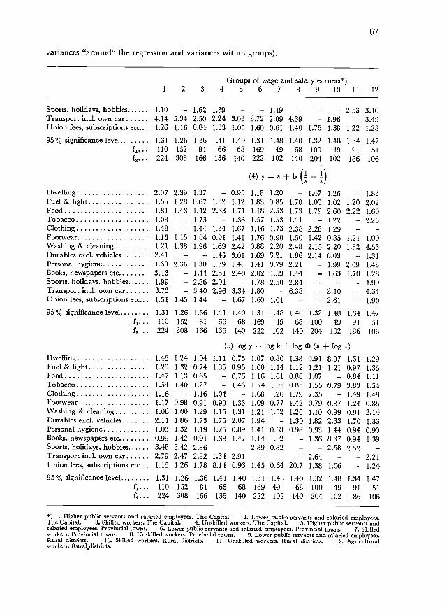
variances "around" the regression and variances within groups).

67

*) 1. Higher public servants and salaried employees. The Capital. 2. Lower public servants and salaried employees.The Capital. 3. Skilled workers. The Capital. 4. Unskilled workers. The Capital. 5. Higher public servants andsalaried employees. Provincial towns. 6. Lower public servants and salaried employees. Provincial towns. 7. Skilledworkers. Provincial towns. 8. Unskilled workers. Provincial towns. 9. Lower public servants and salaried employees.Rural districts. 10. Skilled workers. Rural districts. II. Unskilled workers. Rural districts. 12. Agriculturalworkers. Rural districts.

1 2 3 4Groups of wage and salary earners*)

5 6 7 8 9 10 11 12

Sports, holidays, hobbies 1.10 - 1.62 1.39 - - 1.19 - - - 2.53 3.10Transport incl, own car 4.14 5.34 2.50 2.24 3.03 3.72 2.09 4.39 - 1.96 - 3.49Union fees, subscriptions etc 1.26 1.16 0.84 1.33 1.05 1.60 0.61 1.40 1.76 1.38 1.22 1.28

95% significance level 1.31 1.26 1.36 1.41 1.40 1.31 1.48 1.40 1.32 1.48 1.34 1.47f1 110 152 81 66 68 169 49 68 100 49 91 51f2 224 308 166 136 140 222 102 140 204 102 186 106

(4) y = a + b ( - 1)

Dwelling 2.07 2.39 1.37 - 0.95 1.18 1.20 - 1.47 1.26 - 1.83Fuel & light 1.55 1.28 0.67 1.32 1.12 1.83 0.85 1.70 1.00 1.02 1.20 2.02Food 1.81 1.43 1.42 2.33 1.71 1.18 2.53 1.73 1.79 2.60 2.22 1.60Tobacco 1.08 - 1.73 - 1.36 1.57 1.53 1.41 - 1.22 - 2.25Clothing 1.48 - 1.44 1.34 1.67 1.16 1.73 2.38 2.28 1.29 - -Footwear 1.15 1.15 1.04 0.91 1.41 1.76 0.90 1.50 1.42 0.85 1.21 1.00Washing & cleaning 1.21 1.38 1.96 1.69 2.42 0.88 2.20 2.48 2.15 2.20 1.82 4.53Durables excl, vehicles 2.41 - -. 1.45 3.01 1.69 3.21 1.86 2.14 6.03 -. 1.31Personal hygiene 1.60 2.36 1.30 1.39 1.48 1.41 0.79 2.21 - 1.99 2.09 1.43Books, newspapers etc. 3.13 - 1.44 2.51 2.40 2.02 1.59 1.44 -. 1.63 1.70 1.28Sports, holidays, hobbies 1.99 - 2.86 2.01 - 1.78 2.50 2.84 - - - 4.99Transport incl, own car 3.73 - 3.40 2.96 3.34 1.80 - 6.38 - 3.10 - 4.34Union fees, subscriptions etc.. . 1.51 1.45 1.44 - 1.67 1.60 1.01 - - 2.61 - 1.9095% significance level 1.31 1.26 1.36 1.41 1.40 1.31 1.48 1.40 1.32 1.48 1.34 1.47

f1 110 152 81 66 68 169 49 68 100 49 91 51f5 224 308 166 136 140 222 102 140 204 102 186 106

(5) log y = log k + log t (a + log x)Dwelling 1.45 1.24 1.04 1.11 0.75 1.07 0.80 1.38 0.91 8.07 1.31 1.29Fuel & light 1.29 1.32 0.74 1.85 0.95 1.00 1.14 1.12 1.21 1.21 0.97 1.35Food 1.47 1.13 0.65 0.76 1.16 1.61 0.80 1.07 - 0.84 1.11Tobacco 1.54 1.40 1.27 1.43 1.54 1.05 0.85 1.55 0.79 3.83 1.54Clothing 1.16 - 1.16 1.04 - 1.08 1.20 1.79 7.35 - 1.49 1.49Footwear 1.17 0.98 0.91 0.90 1.33 1.09 0.77 1.42 0.79 0.87 1.24 0.85Washing & cleaning 1.06 1.00 1.29 1.15 1.31 1.21 1.52 1.20 1.10 0.99 0.91 2.14Durables excl, vehicles 2.11 1.86 1.73 1.75 2.07 1.94 - 1.30 1.82 2.33 1.70 1.33Personal hygiene 1.03 1.32 1.19 1.25 0.89 1.41 0.63 0.98 0.93 1.44 0.94 0.90Books, newspapers etc. 0.99 1.42 0.91 1.38 1.47 1.14 1.02 - 1.36 8.37 0.94 1.39Sports, holidays, hobbies 3.48 3.42 2.86 - - 2.89 0.82 - - 2.58 2.52 -Transport incl, own car 2.79 2.47 2.82 1.34 2.91 - - - 2.64 - - 2.21Union fees, subscriptions etc 1.15 1.26 1.78 8.14 0.93 1.45 0.64 20.7 1.38 1.06 1.24

95% significance level .. 1.31 1.26 1.36 1.41 1.40 1.31 1.48 1.40 1.32 1.48 1.34 1.47f1... 110 152 81 66 68 169 49 68 100 49 91 51f2... 224 308 166 136 140 222 102 140 204 102 186 106

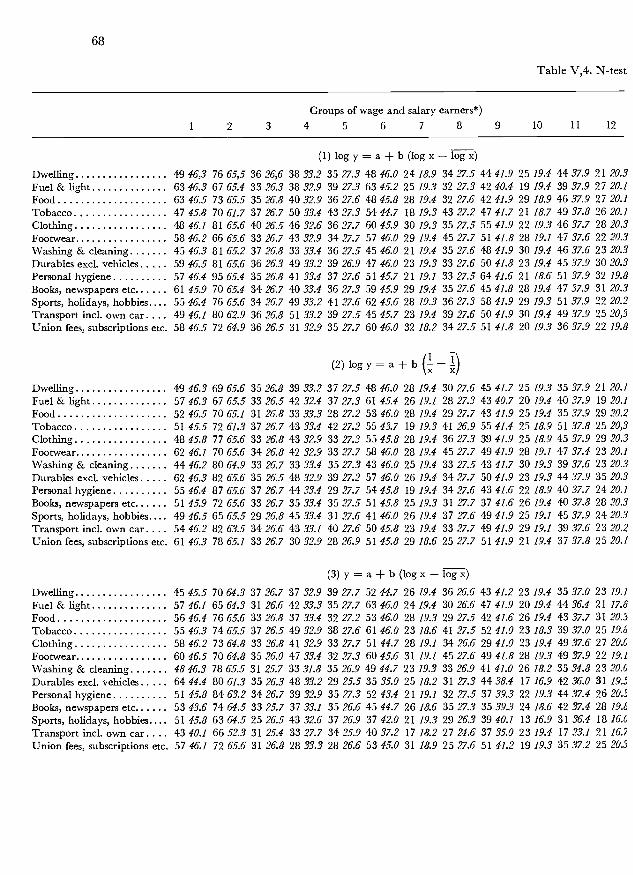
68

Table V,4. N-test

Groups of wage and salary earners*)1 2 3 4 5 6 7 8 9 10 11 12

(1) log y = a + b (log x - log x)

Dwelling 49 46,3 76 65,5 36 26,6 38 33.2 35 27.3 48 46.0 24 18.9 34 27.5 44 41.9 25 19.4 44 37.9 21 20.3Fuel & light 63 46.3 67 65.4 33 26.3 38 32.9 39 27.3 63 45.2 25 19.3 32 27.3 42 40.4 19 19.4 39 37.9 27 20.1Food 63 46.5 73 65.5 35 26.8 40 32.9 36 27.6 48 45.8 28 19.4 32 27.6 42 41.9 29 18.9 46 37.9 27 20.1Tobacco 47 45.8 70 61.7 37 26.7 50 33.4 43 27.3 54 44.7 18 19.3 43 27.2 47 41.7 21 18.7 49 37.8 26 20.1Clothing 48 46.1 81 65.6 40 26.5 46 32.6 36 27.7 60 45.9 30 19.3 35 27.5 55 41.9 22 19.3 46 37.7 28 20.3Footwear 58 46.2 66 65.6 33 26.7 43 32.9 34 27.7 57 46.0 29 19.4 45 27.7 51 41.8 28 19.1 47 37.6 22 20.3Washing & cleaning 45 46.3 81 65.2 37 26.8 33 33.4 36 27.5 45 46.0 21 19.4 35 27.6 48 41.9 30 19.4 46 37.6 23 20.3Durables excl, vehicles 59 46.5 81 65.6 36 26.3 49 33.2 39 26.9 47 46.0 23 19.3 33 27.6 50 41.8 23 19.4 45 37.9 30 20.3Personal hygiene 57 46.4 95 65.4 35 26.8 41 33.4 37 27.6 51 45.7 2119.1 33 27.5 6441.6 21 18.6 51 37.9 32 19.8Books, newspapers etc 61 45.9 70 65.4 34 26.7 40 33.4 36 27.3 59 45.9 29 19.4 35 27.6 45 41.8 28 19.4 47 37.9 31 20.3Sports, holidays, hobbies 55 46.4 76 65.6 34 26.7 49 33.2 41 27.6 62 45.6 28 19.3 36 27.3 58 41.9 29 19.3 51 37.9 22 20.2Transport incl, own car. . 49 46.1 80 62.9 3626.8 51 33.2 3927.5 45 45.7 23 19.4 39 27.6 50 41.9 30 19.4 49 37.9 25 20,3Union fees, subscriptions etc 58 46.5 72 64.9 36 26.5 31 32.9 35 27.7 60 46.0 32 18.2 34 27.5 51 41.8 20 19.3 36 37.9 22 19.8

(2) logy = a + b ( - I)

Dwelling 49 46.3 69 65.6 35 26.8 39 33.2 37 27.5 48 46.0 28 19.4 30 27.6 45 41.7 25 19.3 35 37.9 21 20.1Fuel & light 57 46.3 67 65.5 33 26.5 42 32.4 37 27.3 61 45.4 26 19.1 28 27.3 43 40.7 20 19.4 40 37.9 19 20.1Food 52 46.5 70 65.1 31 26.8 33 33.3 28 27.2 53 46.0 28 19.4 29 27.7 43 41.9 25 19.4 35 37.9 29 20.2Tobacco 51 45.5 72 61.3 37 26.7 43 33.4 42 27.2 55 43.7 19 19.3 41 26.9 55 41.4 25 18.9 51 37.8 25 20,3Clothing 48 45.8 77 65.6 33 26.8 43 32.9 33 27.3 55 45.8 28 19.4 36 27.3 39 41.9 25 18.9 45 37.9 29 20.3Footwear 62 46.1 70 65.6 34 26.8 42 32.9 33 27.7 58 46.0 28 19.4 45 27.7 49 41.9 28 19.1 47 37.4 23 20.1Washing & cleaning 44 46.2 80 64.9 33 26.7 33 33.4 35 27.3 43 46.0 25 19.4 33 27.5 43 41.7 30 19.3 39 37.6 23 20.3Durables excl, vehicles 62 46.3 82 65.6 35 26.5 48 32.9 39 27.2 57 46.0 26 19.4 34 27.7 50 41.9 23 19.3 44 37.9 35 20.3Personal hygiene 55 46.4 87 65.6 37 26.7 44 33.4 29 27.7 54 45.8 19 19.4 34 27.6 43 41.6 22 18.9 40 37.7 24 20.1Books, newspapers etc. 51 45.9 72 65.6 33 26.7 35 33.4 35 27.5 51 45.8 25 19.3 31 27.7 37 41.6 26 19.4 40 37.8 28 20.3Sports, holidays, hobbies 49 46.5 65 65.5 29 26.8 45 33.4 31 27.6 41 46.0 26 19.4 37 27.6 49 41.9 25 19.1 45 37.9 24 20.3Transport incl, own car. . 5446.2 82 63.5 3426.6 43 33.1 4027.6 5045.8 23 19.4 33 27.7 4941.9 29 19.1 39 37.6 23 20.2Union fees, subscriptions etc 61 46.3 78 65.1 33 26.7 30 32.9 28 26.9 51 45.8 29 18.6 25 27.7 51 41.9 21 19.4 37 37.8 25 20.1

(3)y=a+ b(logx-logx)Dwelling 45 455 70 64.3 37 26.7 37 32.9 39 27.7 52 44.7 26 19.4 36 26.6 43 41.2 23 19.4 35 37.0 23 19.1Fuel & light 57 46.1 65 64.3 31 26.6 42 33.3 35 27.7 63 46.0 24 19.4 30 26.6 47 41.9 20 19.4 4436.4 2117.8Food 56 46.4 76 65.6 33 26.8 37 33,4 32 27.2 53 46.0 28 19.3 29 27.5 42 41.6 26 19.4 43 37.7 31 20.3Tobacco 55 46.3 74 65.5 37 26.5 49 32.9 38 27.6 61 46.0 23 18.6 41 27.5 52 41.0 23 18.3 39 37.0 25 19.6Clothing 58 46.2 73 64.8 33 26.8 41 32.9 33 27.7 51 44.7 28 19.1 34 26.6 29 41.0 23 19.4 49 37.6 27 20.6Footwear 60 46.5 70 64.8 35 26.0 47 33.4 32 27.3 60 45.6 31 19.1 45 27.6 49 41.8 28 19.3 49 37.9 22 19.1Washing & cleaning 4846.3 78 65.5 31 25.7 33 31.8 35 26.9 49 44.7 23 19.3 33 26.9 41 41.0 26 18.2 35 34.8 23 20.6Durables excl. vehicles 64 44.4 80 61.3 35 26.3 48 33.2 29 255 35 350 25 18.2 31 27.3 44 38.4 17 16.9 42 36.0 31 19.3Personal hygiene 51 458 84 63.2 3426.7 39 32.9 35 27.3 52 43.4 2119.1 32 27.5 37 39.3 22 19.3 4437.4 26 20.1Books, newspapers etc. 53 43.6 74 64.5 33 257 37 33.1 35 26.6 45 44.7 26 18.6 35 27.3 35 39.3 24 18.6 42 37.4 28 19.6Sports, holidays, hobbies 51 45.8 63 64.5 25 26.5 43 32.6 37 26.9 37 42.0 2119.3 29 26.3 39 40.1 13 16.9 31 36.4 18 16.6Transport incl, own car. . 43 40.1 6652.3 31 254 33 27.7 34259 40 37.2 17 18.2 27 24.6 37 350 23 19.4 17 23.1 21 16.2Union fees, subscriptions etc. 57 46.1 72 656 31 26.8 28 33.3 28 26.6 53 450 31 18.9 25 27.6 51 41.2 19 19.3 3537.2 25 20.

br number of runs.*)

Groups of wage and salary earners*)1 2 3 4 5 6 7 8 9 10 11 12

(4) y = a + b -)welling 43 45.3 55 63.2 27 26.5 37 32.4 27 27.5 39 44.7 24 18.2?uel & light 49 44.0 61 63.5 36 26.6 36 33.3 33 27.5 63 45.0 24 19.4ood 50 45.8 60 65.4 19 26.8 19 33.3 20 23.4 35 45.2 21 18.6

['obacco 61 45.9 72 65.4 31 25.4 37 31.8 30 25.9 49 44.7 23 19.11othing 49 46.2 61 63.5 29 26.8 33 33.4 25 27.2 43 43.7 21 19.3ootwear 58 46.5 65 64.9 34 26.3 39 33.4 35 27.6 55 45.0 29 19.3

ATashing & cleaning 46 46.2 61 64.8 31 26.0 29 31.4 29 25.5 35 42.5 19 18.2)urables excl, vehicles 62 43.6 71 61.7 31 25.0 42 32.9 27 25.1 36 37.2 23 17.8ersona1 hygiene 37 43.2 57 59.9 35 26.6 35 32.6 27 26.9 39 42.0 17 19.3

3ooks, newspapers etc 49 43.6 74 62.4 25 24.6 37 32.4 21 259 31 37.2 23 19.1;ports, holidays, hobbies 39 44.7 55 61.7 15 26.3 31 33.2 33 26.3 33 38.0 19 18.2L'ransport incl, own car. 45 41.2 5851.5 2925.0 29 27.7 28 24.6 3635.0 17 15.7Jnion fees, subscriptions etc 51 46.1 74 65.1 23 26.6 26 33.2 29 25.9 47 45.2 27 19.4

28 25121 26.927 27.531 26.331 26.637 26.632 26.321 26.921 27.227 26.927 25.123 25.121 26.6

69

31 37.040 35.727 35.439 35.437 33.845 37.931 34.342 35431 37.035 37.027 30.719 24.129 357

23 19.517 19.823 19.521 19.523 18.821 19.521 19.133 19.516 19.127 19.817 17.317 16.023 19.1

) The italicized figures denotes the lower 5 per cent significance level. I. Higher public servants and salaried employees. The Capital. 2. Lower publicervants and salaried employees. The Capital. 3. Skilled workers. The Capital. 4. Unskilled workers, The Capital. 5. Higher public servantsnd salaried employees. Provincial towns. 6. Lower public servants and salaried employees. Provincial towns. 7. Skilled workers. Provincial towns,

Unskilled workers. Provincial towns. 9. Lower public servants and salaried employees. Rural districts, 10 Skilled workers. Rural districts.1. Unskilled workers. Rural districts. 12, Agricultural workers. Rural districts.

(5) log y = log k + log (a + log x))welling 53 46.1 78 656 37 26.5 38 33.2 34 27.3 48 46.0 26 19.1 32 27.5 44 41.9 1118.6 44 37.9 21 20.3ue1 & light 61 46.1 67 65.1 33 26.5 38 33.1 37 27.5 65 450 25 19.3 32 27.3 42 40.4 19 19.4 41 37.7 27 20.1

?ood 63 46.4 75 65.4 34 26.8 - - 34 27.7 53 46.0 28 19.4 34 27.5 44 41.9 - - 46 37.8 2920.3Fobacco 49 45.9 70 62.1 37 26.7 - - 43 27.2 54 44.1 18 19.3 44 26.9 51 41.4 25 19.0 33 37.9 28 20.3lothing 50 46.3 - - 40 26.5 48 32.9 - - 60 459 30 19.3 38 27.5 31 40.1 - - 46 37.8 28 20.2

?Ootwear 60 46.2 66 65.6 33 26.7 41 32.9 34 27.7 58 46.0 29 19.4 45 27.7 49 41.9 28 19.1 47 37.4 22 20.3?Vashing & cleaning 46 46.2 82 651 37 26.8 31 33.2 36 27.6 46 46.0 21 19.4 35 27.6 47 41.9 30 19.4 48 37.7 23 20.3)urables excl, vehicles 61 46.5 81 65.6 36 26.3 49 33.2 39 27.2 47 46.0 - - 33 27.7 52 41.6 23 19.4 45 37.9 30 20.2ersonal hygiene 55 46.4 94 65.5 36 26.7 41 33.4 39 27.7 49 46.0 23 19.4 33 27.6 62 41.6 21 18.6 47 37.9 32 19.8ooks, newspapers etc 59 45.9 70 655 34 26.7 38 33.4 36 27.3 55 46.0 29 19.4 - 42 41.8 15 19.4 49 37.9 31 20.3ports, holidays, hobbies 33 46.1 51 656 29 26.8 - - - - 45 46.0 28 19.4 - - - 27 19.4 33 37.8L'ransport incl, own car. 51 46.2 82 62.8 37 26.8 51 33.2 39 27.5 ------42 41.9 - - - - 25 20.3Jnion fees, subscriptions etc. 63 46.5 76 64.3 15 26.6 25 32.9 35 27.6 62 46.0 34 18.6 19 27.5 53 41.8 22 19.4 - - 24 20.1

35 40.7 17 18.233 41.0 24 19.133 41.0 17 19.453 40.7 25 18.023 39.7 19 18.943 41.0 25 19.437 39.3 17 16.941 37.9 15 16.333 38.9 2119.435 36.3 24 19.133 357 15 16.327 31.4 2118.939 40.1 15 18.2

i (y) =

The F-values thus calculated have been shown in table V,3.Can any conclusions be drawn from the F-test as regards the determination of the

"best" algebraic formulation(s) of the Engel curve? Does the F-test point in the samedirection as the X2-test and as the more dubious evidence from the correlation coefficients,i.e. to one of those functions in which the dependent variable is the logarithmicallytransformed expenditure, log y?

As mentioned above there are several reservations to be made. For expenditureitems where > 0.5 the F-test fades away as regards functions (1,1), (1,2), and (1,5). Asregards functions (1,3) and (1,4), parameter estimation has failed in some cases, cf.chapter IV, p. 54, and, accordingly, no testing is possible. These cases coincide with theinvalidation due to high a-values of the F-test performed on functions (1,1) and (1,2).Despite these substantial reservations concerning the results shown in the table, itnevertheless seems justified to draw the general conclusion that the F-test confirms theconclusion of the 2-test to the effect that the logarithmic functions pass the testsmore easily than the functions in which the expenditure enters untransformed.

For all expenditure items (except footwear) there are significant F-values for all fivetypes of functions in one ore more of the twelve social groups, but in the case of functions(1,1) and (1,2) frequently only one of the social groups gives significance. For the double-logarithmic function (1,1) the items of dwelling and footwear and fuel and lighting thus show

70

where ni = 3 is the number of observations in the j'th group. s22 has been calculated

direct on the basis of [log y - f(x)] and (Y ), respectively for the two types of

functions.As regards s2 it has not been possible to use the individual observations in those

cases where log Y was the dependent variable since several observations of Y were zero.This zero-observation problem, which was apparently solved by the grouping of theobservations, cf. the discussion in chapter IV, p. 36, thus crops up again here in a new

form. However, for moderate values of the average coefficient of variation = 8y12

si2, may be found with good approximation as (log y) M2 . , where M = 0.4343.This approximation is not very good in those cases where > 0.5, which must be

borne in mind when the F-tests are examined below. For the three items durable goods,transport and sports, holidays and hobbies several of the calculated c-values are very high,and the F-test in the case of these items must be considered dubious as regards the twofunctions in which log y is the dependent variable.

As regards the functions in which y is the dependent variable, s2 has everywhere beenconsidered equal to , since

71

only one significant F-value, food, house-cleaning and washing, two significant values, andclothing, personal hygiene, sports, holidays and hobbies, and subscriptions, etc. three significantvalues. The semi-logarithmic function (1,2) displays somewhat poorer results. For theremaining functions the number of significant results are much higher.

4. The test for number of runs and for the longest run; the d-test.

The last category of tests for goodness of fit tests the hypothesis that the observationsare distributed at random around the Engel curve determined by the calculated para-meter estimates.

The two runs test consist of a simple count of the number of changes of signs (testfor number of runs, here called N-test) and of the number of elements in the longestrun (test for longest run, here called l-test). A run is accordingly defined as a series ofsuccessive deviations with the same sign, cf. e.g. A. Hald, (8), p. 342, and Prais andHouthakker, (10), pp. 53-55. If the number of positive and negative deviations, P andQ, respectively are greater than about ten, D is approximately normally distributed

with mean M D F i + 2 PQ

2PQ(2PQN)and variance V DF N2 (N - 1)where D is number of runs and N the number of observations.

If the test hypothesis is rejected in favour of an alternative hypothesis because thecalculated Engel curve "misses the mark" in a greater or smaller area of the field ofobservation, then the number of runs will be too small.

The limit of significance can be chosen as

M{D.-2VV{DFIn table V,4 the number of runs, D, and the limit of significance thus found has been

shown.The test for the longest run, the l-test, which is not, of course, unrelated to the N-test,

is derived from the knowledge of the distribution function for the number of runs of agiven length.

In table V,6 all the longest runs have been shown, and for each set of calculationshas been given the 5 per cent significance limit.

A glance at table V,4 and table V,5 will show how the results of the two tests of runscorrespond so that they should rightly be considered as one test. The conclusion ofthis combined test points in the same direction as the previous tests: among the fiverelations tested the two in which the dependent variable is a logarithmic transformationof the expenditure performs better than the other three functions, and as indicated alsoby the F-test, the double-logarithmic function seems to do best.

The final test, the d-test, is based on the following quantity, cf. Prais and Houthakker(10), page 53

d = E (tk tk )2/E tk2

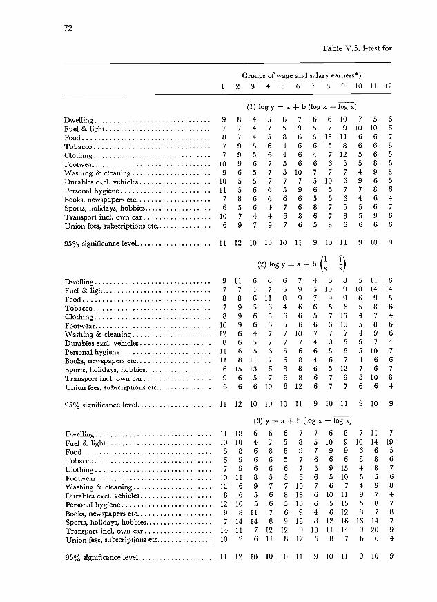
72

Table V,5. l-test for

1 2

Groups of wage and salary earners*)3 4 5 6 7 8 9 10 11 12

(1)logy=a+ b(logxlogx)Dwelling 9845676610756FueI&light 77475957910106Food 8 7 4 5 8 6 5 13 11 6 6 7

Tobacco 7 9 5 6 4 6 6 5 8 6 6 8Clothing 7956464712565Footwear 10 9 6 7 5 6 6 6 5 5 8 5

Washing & cleaning 9 6 5 7 5 10 7 7 7 4 9 8Durables excl, vehicles 10 5 5 7 7 7 5 10 6 9 6 5

Personal hygiene 11 5 6 6 5 9 6 5 7 7 8 6

Books, newspapers etc. 7 8 6 6 6 6 5 5 6 4 6 4Sports, holidays, hobbies 6 5 6 4 7 6 8 7 5 5 6 7

Transport incl, own car 10 7 4 4 6 8 6 7 8 5 9 6

Union fees, subscriptions etc. 6 9 7 9 7 6 5 8 6 6 6 6

95% significance level 11 12 10 10 10 11 9 10 11 9 10 9

(2) logy = a + b ( -Dwelling 9 11 6 6 6 7 4 6 8 5 11 6

Fuel&light 7747595109101414Food 8 8 6 11 8 9 7 9 9 6 9 5

Tobacco 7 9 5 6 4 6 6 5 6 5 8 6

Clothing 8965665715474Footwear 10966566610586Washing & cleaning 12 6 4 7 7 10 7 7 7 4 9 6

Durables excl, vehicles 8 6 5 7 7 7 4 10 5 9 7 4

Personal hygiene 11 6 5 6 5 6 6 5 8 5 10 7

Books, newspapers etc 11 8 11 7 6 8 4 6 7 4 6 6

Sports, holidays, hobbies 6 15 13 6 8 8 6 5 12 7 6 7

Transport incl, own car 9 6 5 7 6 8 6 7 9 5 10 8

Union fees, subscriptions etc. 6 6 6 10 8 12 6 7 7 6 6 4

95% significance level 11 12 10 10 10 11 9 10 11 9 10 9

(3) y = a + b (log x - log x)

Dwelling 11 18 6 6 6 7 7 6 8 7 11 7

Fuel & light 10 10 4 7 5 8 5 10 9 10 14 19

Food 886889799665Tobacco 6 9 6 6 5 7 6 6 6 8 8 6

Clothing 7966675915487Footwear 10 11 8 5 5 6 6 5 10 5 5 6

Washing & cleaning 12 6 9 7 7 10 7 6 7 4 9 8Durables excl, vehicles 8 6 5 6 8 13 6 10 11 9 7 4Personal hygiene 12 10 5 6 5 10 6 5 15 5 8 7

Books, newspapers etc. 9 8 11 7 6 9 4 6 12 8 7 8

Sports, holidays, hobbies 7 14 14 8 9 13 8 12 16 16 14 7

Transport incl, own car 14 11 7 12 12 9 10 11 14 9 20 9

Union fees, subscriptions etc. 10 9 6 11 8 12 5 8 7 6 6 4

95% significance level 11 12 10 10 10 11 9 10 11 9 10 9

the longest run.

73

*) 1. Higher public servants and salaried employees. The Capital. 2. Lower public servants and salaried employees.The Capital. 3. Skilled workers. The Capital. 4. Unskilled workers. The Capital. 5. Higher public servants andsalaried employees. Provincial towns. 6. Lower public servants and salaried employees. Provincial towns. 7. Skilledworkers. Provincial towns. 8. Unskilled workers. Provincial towns. 9. Lower public servants and salaried employees.Rural districts. 10. Skilled workers. Rural districts. Il. Unskilled workers. Rural districts. 12. Agriculturalworkers. Rural districts.

Groups of wage and salary earners*)1 2 3 4 5 6 7 8 9 10 11 12

(4) y = a + b ( - I)

Dwelling 11 21 11 6 12 11 7 7 14 12 11 9Fuel & light 10 11 4 10 8 11 6 16 19 9 15 19Food 8 20 13 17 26 21 16 10 23 13 17 10Tobacco 6 9 9 10 10 11 6 8 8 9 10 10Clothing 12 17 7 10 13 18 7 11 24 9 9 7Footwear 101687556614696Washing & cleaning 12 15 9 15 13 17 7 10 10 7 13 8Durables excl, vehicles 8 9 8 9 13 13 7 11 11 11 7 4Personal hygiene 15 31 6 9 10 18 7 17 15 6 12 19Books, newspapers etc. 10 8 11 7 11 17 5 10 13 8 14 8Sports, holidays, hobbies 11 14 20 11 9 15 8 10 15 16 14 7Transport incl, own car 14 13 7 14 13 9 10 11 14 12 22 12

Union fees, subscriptions etc. 10 8 15 11 8 16 6 14 14 15 15 8

95% significance level 11 12 10 10 10 11 9 10 11 9 10 9

(5) log y = log k + log (a + log x)

Dwelling 98456746102456Fuel&light 7 7 4 7 5 9 5 7 9 10 11 6Food 876-875910-65Tobacco 795-466585184Clothing 7-55-64717-65Footwear 10 9 6 7 5 6 6 6 9 5 8 5Washing & cleaning 9 6 5 10 5 10 7 7 7 4 9 8Durables excl, vehicles 6 5 5 7 7 7 - 10 5 9 6 5Personal hygiene 11 5 6 6 5 5 6 5 7 7 8 6Books, newspapers etc 7 8 6 7 6 6 5 - 6 14 6 4Sports, holidays, hobbies 21 23 13 - - 12 8 - - 7 19 -Transport incl, own car 9 7 5 4 6 - - - 11 - - 6Union fees, subscriptions etc. 6 9 17 18 7 5 5 20 6 6 - 4

95% significance level 11 12 10 10 10 11 9 10 11 9 10 9

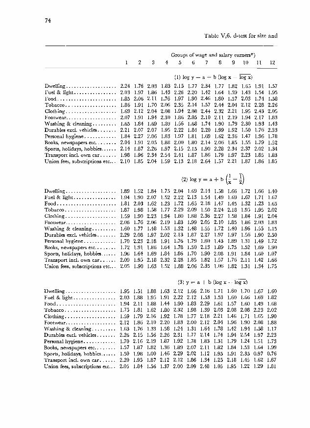
74

Table V,6. d-test for size and

1 2 3 4Groups of wage and salary earners*)

5 6 7 8 9 10 11 12

(1) log y a + b (log x - log x)Dwelling 2.24 1.76 2.03 1.83 2.15 1.77 2.34 1.77 1.82 1.65 1.91 1.57Fuel & light 2.03 1.97 1.86 1.43 2.26 2.20 1.42 1.64 1.59 1.43 1.54 1.95Food 1.85 2.06 2.11 1.76 1.97 1.90 2.46 1.80 1.57 2.03 1.74 1.58Tobacco 1.86 1.91 1.70 2.06 2.35 2.14 1.57 2.44 2.04 2.12 2.28 2.26Clothing 1.69 2.12 2.04 2.08 1.94 2.08 2.44 2.32 2.21 1.95 2.43 2.05Footwear 2.07 1.91 1.94 2.30 1.86 2.05 2.10 2.11 2.19 1.94 2.17 1.83Washing & cleaning 1.65 1.84 1.69 1.89 1.56 1.68 1.74 1.90 1.79 2.30 1.93 1.43Durables excl, vehicles 2.21 2.07 2.07 1.95 2.22 1.84 2.20 1.99 1.92 1.50 1.76 2.33Personal hygiene 1.84 2.27 2.06 1.83 1.97 1.81 1.69 1.62 2.36 1.47 1.96 1.78Books, newspapers etc. 2.04 1.91 2.05 1.88 2.00 1.80 2.14 2.06 1.85 1.55 1.79 1.52Sports, holidays, hobbies 2.14 1.87 2.26 1.97 2.15 2.15 1.90 2.28 2.34 2.37 2.02 1.34Transport incl, own car 1.98 1.96 2.34 2.54 2.41 1.87 1.86 1.79 1.97 2.23 1.85 1.83Union fees, subscriptions etc.. . 2.10 1.85 2.04 1.59 2.13 2.18 2.64 1.57 2.21 1.87 1.86 1.85

(1 1(2) log y = a + b ii

Dwelling 1.89 1.52 1.84 1.75 2.04 1.69 2.14 1.58 1.66 1.72 1.66 1.40Fuel & light 1.94 1.90 2.07 1.52 2.22 2.13 1.54 1.49 1.69 1.67 1.71 1.67Food 1.81 2.03 1.62 1.23 1.72 1.65 2.18 1.47 1.45 1.32 1.23 1.65Tobacco 1.87 1.98 1.58 1.77 2.29 2.09 1.50 2.24 2.18 1.95 1.95 2.02Clothing 1.59 1.90 2.23 1.94 1.80 1.88 2.36 2.27 1.58 1.84 1.91 2.04Footwear 2.06 1.76 2.06 2.19 1.83 1.99 2.05 2.10 1.85 1.86 2.03 1.83Washing & cleaning 1.60 1.77 1.48 1.53 1.32 1.48 1.55 1.72 1.40 1.96 1.55 1.15Durables excl, vehicles 2.29 2.08 1.97 2.02 2.13 1.87 2.27 1.97 1.97 1.56 1.90 2.50Personal hygiene 1.70 2.23 2.18 1.91 1.76 1.79 1.80 1.43 1.89 1.31 1.49 1.72Books, newspapers etc. 1.72 1.91 1.86 1.64 1.78 1.50 2.13 1.89 1.75 1.52 1.69 1.90Sports, holidays, hobbies 1.96 1.64 1.69 1.84 1.86 1.70 1.90 2.08 1.91 1.84 1.60 1.07Transport incl, own car 2.09 1.95 2.18 2.32 2.28 1.85 1.82 1.57 1.76 2.11 1.42 1.66Union fees, subscriptions etc.. . 2.05 1.90 1.63 1.52 1.88 2.06 2.35 1.06 1.82 1.31 1.34 1.75

(3)y==a+b(logx-logxDwelling 1.95 1.51 1.88 1.63 2.12 1.66 2.16 1.71 1.60 1.70 1.67 1.60Fuel & light 2.03 1.88 1.95 1.91 2.22 2.12 1.53 1.53 1.60 1.66 1.69 1.82Food 1.94 2.11 1.88 1.44 1.90 1.83 2.29 1.61 1.57 1.60 1.49 1.68Tobacco 1.75 1.81 1.62 1.80 2.32 1.98 1.39 2.03 2.08 2.08 2.23 2.02Clothing 1.59 1.79 2.16 1.92 1.78 1.77 2.18 2.21 1.46 1.71 1.65 1.90Footwear 2.12 1.86 2.10 2.20 1.83 2.00 2.12 2.04 1.96 1.90 2.08 1.88Washing & cleaning 1.63 1.76 1.33 1.58 1.24 1.31 1.64 1.78 1.42 1.94 1.58 1.17Durables excl, vehicles 2.26 2.15 1.56 2.26 2.31 1.77 2.14 1.74 1.94 2.54 1.97 2.23Personal hygiene 1.70 2.16 2.19 1.87 1.92 1.78 1.83 1.31 1.79 1.24 1.51 1.73Books, newspapers etc. 1.57 1.87 1.82 1.36 1.89 2.07 2.11 1.82 1.84 1.53 1.64 1.99Sports, holidays, hobbies 1.50 1.98 1.00 1.46 2.29 2.02 1.12 1.95 1.91 2.35 0.97 0.76Transport incl, own car 2.20 1.95 1.87 2.12 2.12 1.86 1.34 1.25 2.18 1.45 1.62 1.67Union fees, subscriptions etc.. . 2.05 1.84 1.56 1.37 2.00 2.09 2.48 1.05 1.95 1.22 1.29 1.81

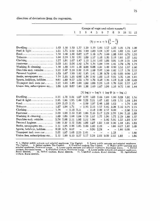
direction of deviations from the regression.

75

Groups of wage and salary earners*)1 2 3 4 5 6 7 8 9 10 11 12

(4) y = a + b ( -Dwelling 1.43 1.18 1.53 1.77 1.50 1.18 1.66 1.57 1.22 1.31 1.73 1.39Fuel & light 1.61 1.75 2.02 1.86 1.90 1.83 1.64 1.37 1.41 1.82 1.35 1.47Food 1.50 1.68 1.02 0.82 1.27 1.18 1.71 1.00 1.08 0.81 0.70 1.20Tobacco 1.64 2.20 1.32 1.91 1.89 1.57 1.18 1.35 2.14 1.81 1.37 1.65Clothing 1.22 1.91 1.67 1.47 1.13 1.16 1.63 1.86 0.91 1.19 2.31 1.94Footwear 2.03 1.61 2.06 1.92 1.74 1.76 1.88 1.94 1.41 1.70 1.78 1.73Washing & cleaning 1.34 1.39 1.01 1.18 0.89 0.88 1.31 1.49 0.99 1.51 1.07 1.00Durables excl, vehicles 2.22 2.07 2.10 2.02 2.16 1.69 2.02 1.50 1.82 1.17 1.78 2.12Personal hygiene 1.35 1.67 1.99 1.62 1.35 1.41 1.58 0.79 1.45 0.85 0.90 1.37Books, newspapers etc. 1.16 2.35 1.55 0.98 1.34 2.02 1.83 1.13 2.01 1.35 1.28 1.85Sports, holidays, hobbies 0.81 1.99 0.57 1.05 1.73 1.78 0.53 1.36 1.23 2.19 1.38 0.49Transport incl. own car 2.22 1.66 1.49 1.84 1.98 1.80 2.24 1.10 1.78 0.91 2.27 1.47Union fees, subscriptions etc.. 1.86 1.56 0.87 1.86 1.38 1.60 1.67 1.94 1.54 0.72 1.66 1.44

(5) log y = log k + log I1 (a ± log x)Dwelling 2.21 1.78 2.01 1.87 2.22 1.83 2.45 1.80 1.90 0.29 1.92 1.56Fuel & light 2.05 1.96 1.95 1.48 2.28 2.21 1.47 1.82 1.63 1.51 1.64 1.94Food 1.93 2.13 2.15 - 2.09 1.97 2.48 1.88 1.65 - 1.74 1.69Tobacco 1.87 1.94 1.71 - 2.35 2.15 1.57 2.45 2.09 2.10 0.75 2.25Clothing 1.74 - 2.13 2.11 - 2.13 2.49 2.57 0.30 - 2.38 2.15Footwear 2.09 1.90 2.10 2.33 1.86 2.10 2.17 2.29 2.20 1.96 2.18 1.89Washing & cleaning 1.69 1.86 1.64 1.84 1.53 1.67 1.72 1.96 1.72 2.29 1.88 1.37Durables excl, vehicles 2.24 2.08 2.11 1.98 2.22 1.96 - 2.05 2.05 1.52 1.80 2.37Personal hygiene 1.86 2.32 2.12 2.06 1.98 1.87 1.82 1.69 2.36 1.44 1.95 1.83Books, newspapers etc. 2.11 1.95 2.06 1.85 2.00 1.80 2.19 - 1.86 0.27 1.82 1.69Sports, holidays, hobbies 0.59 0.71 0.67 - - 0.96 2.29 - - 1.46 0.98 -Transport incl, own car 2.02 1.97 1.68 2.55 2.41 - - - 1.53 - - 1.88Union fees, subscriptions etc.. 2.12 1.90 0.10 0.27 2.17 2.24 2.65 0.09 2.22 1.83 - 1.86

*) 1. Higher public servants and salaried employees. The Capital. 2. Lower public servants and salaried employeesThe Capital. 3. Skilled workers. The Capital. 4. Unskilled workers. The Capital. 5. Higher public servants andsalaried employees. Provincial towns. 6. Lower public servants and salaried employees. Provincial towns. 7. Skilledworkers. Provincial towns. 8. Unskilled workers. Provincial towns. 9. Lower public servants and salaried employees.Rural districts. 10. Skilled workers. Rural districts. 11. Unskilled workers. Rural districts. 12. Agriculturalworkers. Rural districts.

Table V,7. Number of significant test results among 12 groups of wage and salary earners. Significance level 95% (y,', F2, 1) and5% (N, d.)

only li test results. only 10 test results. only 9 test results. only 8 test results, only 7 test results. only 6 test results.

logy=a+b(logxlogx)

x' F N x2

logy=a+bQ)

F N 1 d

y=a+b(logxlogx)

' F N

y=a+b()

x2 F N 1

logy=logk+log(a+logx)

d x' F N 1 d1 d I d

Dwelling 0 1 0 0 0 0 5 1 1 2 5 5 2 3 2 6 6' 8 9 8 1 2 1 1 2

Fuel&light 5 1 3 2 5 2 3 4 4 2 5 2 4 4 1 6 4 4 5 4 5 2 2 2 5

Food 1 2 1 2 1 1 5 2 1 5 1 3 2 0 3 4 12 9 11 10 12 22 02 02 12

Tobacco 4 6 1 0 0 3 9 1 0 1 0' 1' 0 0 134 54 2 4 6 31 71 2' 1' 2'

Clothing 1 3 0 0 0 1 4 2 1 2 2 5 2 1 2 33 6' 7 8 6 l 43 l 1' 1'Footwear 1 0 2 0 0 1 0 0 0 0 3 0 0 0 0 2 4 1 2 2 1 1 0 0 0

Washing&cleaning 1 2 2 0 1 1 6 3 2 8 5 7 3 1 8 10 11 8 7 11 0 2 0 0 3

Durables excl, vehicles 1 10 0 2 0 2 10 0 2 0 7' 9' 2 4 173 8 6 5 2 1' 91 0' 0' 1'

Personalhygiene 2 3 0 1 0 2 3 1 2 3 6 3 1 2 3 8' 7' 9 8 8 1 2 0 0 1

Books, newspapers etc 0 4 0 0 0 1 5 2 2 1 6' 51 3 2 2 6 8' 6 6 7 2' 4' 1' 1 1

Sports, holidays, hobbies. . . 1 3 0 0 1 0 6 3 3 3 3 3 5 7 6 66 66 10 10 8 2' 6' 55 55 6

Transport incl, own car 3 11 1 0 0 4 12 0 1 1 82 10' 8 9 3 6 75 10 10 4 3 6 0 0 1

Union fees, subscriptions etc 1 3 1 0 0 1 3 3 2 4 1 3 5 2 5 74 74 6 7 7 31 5 3 3 3

77

where tk is the deviation of the observed from the calculated expenditure on a givenexpenditure item for the k'th group of observations, where the observations are arrangedby increasing values of income.

As in the z2-test it is always the weighted residuals, which are used in the tests forthe two relations in which the untransformed value of the expenditure, y, is the de-pendent variable.

In their article5) Durbin and Watson have examined the distribution function for dand have calculated significance zones for this quantity under alternative assump-tions as regards number of observations (L) and number of parameters in the functionon the basis of which the residuals have been calculated (in this case 2). Durbin andWatson's tables do not allow of any precise delimitation of the level of significance sinced-values within the calculated significance zones do not permit any conclusion as regardsrejection or acceptance of the test hypothesis.

It will be seen from table V,6 and table V,7 that the d-test permits a more preciseconclusion than the run tests. While both function (1,1) and (1,2) pass the N- and l-testsfairly well, the double-logarithmic function getting on the whole the best marks, thed-test reveals the difference between these two functions more clearly.

In a number of cases the semi-logai ithmic function gives d-values which are clearlybeyond the significance zone presumably because the size of the residuals in the firstand in the last run is in certain cases larger than permissibleeven where the numberof elements in these runs (as determined by the shifts of sign) may not be significant.

5. Summary of test results.

In table V,7 a summary of the tests has been given. For each item of expenditure thenumber of significant test results among the twelve social groups has been counted separa-tely for each of the five Engel functions. Bearing in mind the reservations mentionedabove as regards the validity of the different tests, this summary clearly emphasizesthe conclusion which has gradually emerged in the course of the discussion of the indi-vidual tests. The double-logarithmic Engel function gives the best goodness of fit amongthe five functions tested. This does not, of course, mean that the "true" Engel curvefunction have thus been found, but the selection of the double-logarithmic functionas the "best" may, nevertheless, justify a further analysis of the result of the parameterestimation for this function.

Vc. Analysis of estimates of the parameters.

1. Regression analysis versus two-way cross-tabulation.

Table V,8 shows estimates of the standard deviation in the distribution of log y forall 13 expenditure items, separately for each of the 12 social groups. To make it possibleto assess the effect of the introduction of the disposable income x as explanatory variable,estimates of the standard deviation in the distribution of the residuals from the calculated

5) Cf. Durbin and Watson (4).

78

double-logarithmic Engel function have been shown too. It will be seen that the un-explained part of the variation in expenditures, is reduced by 10 to 60 per cent as onegoes from the simple mean value description to the Engel function. The table showsthat the gain is fairly constant from one social group to another for the same expenditureitemwhereas there are great variations among the expenditure items. The size of thegain depends partly on the slope of the Engel curve and partly on the size of the variancewithin groups. If this variance is small, the gain from the regression analysis will, ceterisparibus, be relatively great, and if the regression line is steep, the gain will, ceteris pari bus,also be great.

The food group has a small variance, and even if the slope of the regression line ismoderate a considerable gain is nevertheless achieved through the regression. The itemsports, holidays, hobbies etc., has a relatively high variance, but since the regression linesare rather steep, the gain is also in this case considerable. Expenditures on fuel, light andfootwear rise slowly with income and the variance is substantial; the regression gain isinsignificant. This is also the case of the item of durable goods, where the extremelyhigh variance almost completely counteracts the effect of the fairly steep regressionline.

Another measure of this regression gain is obtained by calculating the ratio of theestimates of the slopes to their estimated standard errors. This is at the same time atest for the hypothesis fi = O, since this hypothesis can be tested by a t-test. The

quantityb O

follows the t-distribution with N-2 degrees of freedom, where N

is the number of group averages included in the calculation of b. The t-values thuscalculated show that the hypothesis = O, i.e. that the slope of the regression line iszero, cannot be accepted in one single case.

It thus seems justified to conclude that the description of the consumption behaviourof the household has gained considerably in precision by the inclusion of the disposablehousehold income as explanatory variable.

By arranging the observations of expenditures in cross-tables where each household isplaced in a cell according to its disposable income, it is often attempted to includedisposable income as an explanatory variable. The frequent use of this type of tables inpublications dealing with household-surveys is often explained by the wish to presentthe material in a clear manner without adopting a definite hypothesis concerning the

form of the relationship between the two variable expenditure and income.The method used here for the description of the expenditure-income relationships,

however, has obvious advantages over this frequently used grouping method. As shownby Amundsen6), information is lost to a considerable extent when the basic materialis split up into the many cells of such a table since only the observations of the individualcell is used in the calculation of the average expenditure figure of this cell.

The parameter estimates have thus made it possible to give a more precise descriptionof the observations than the usual description by averagesbe they overall averagesor "cell averages" in a cross table.

6) Amundsen (2).

Table V,8. Gain of regression. Standard errors in the distribution of expenditures and in the distribution of deviations from thedouble logarithmic Engel function, log y = a + b (log x -

Fuel Washing Durables Peonal Books, Sports, Trans- UnionGroup of wage and salary earners Dwelling &

lightFood Tobacco Clothing Footwear &

cleaningexcl.

vehicleshygiene newspa-

pers etc.holidays,hobbies

port incl.own car

fees,sub-scription

The capitalHigher public servants Slog y 0.23 0.18 0.12 0.29 0.21 0.15 0.20 0.31 0.19 0.24 0.30 0.40 0.17and salaried employees Slog y Ix 0.14 0.12 0.069 0.25 0.13 0.13 0.13 0.29 0.11 0.14 0.13 0.36 0.13

Lower public servants Slog y 0.22 0.20 0.12 0.32 0.25 0.17 0.22 0.36 0.23 0.25 0.31 0.37 0.19

and salaried employees 5log y x. 0.13 0.17 0.067 0.27 0.14 0.12 0.13 0.32 0.12 0.17 0.17 0.31 0.14

Skilled workers Slog y 0.22 0.14 0.14 0.25 0.24 0.14 0.19 0.35 0.17 0.20 0.32 0.43 0.20

Slog y x 0.13 0.12 0.050 0.18 0.13 0.10 0.14 0.26 0.11 0.13 0.13 0.30 0.086

Unskilled workers Slog y . 0.23 0.18 0.15 0.29 0.26 0.17 0.21 0.35 0.21 0.28 0.34 0.38 0.25

Slog y Ix. . 0.14 0.17 0.062 0.20 0.16 0.13 0.14 0.29 0.13 0.18 0.19 0.27 0.13

Provincial towns.Higher public servants 5iog y 0.19 0.16 0.12 0.27 0.22 0.14 0.22 0.37 0.18 0.27 0.33 0.54 0.17

and salaried employees Slog y x 0.11 0.12 0.056 0.22 0.12 0.11 0.15 0.32 0.097 0.17 0.14 0.43 0.093

Lower public servants Slog y 0.23 0.18 0.15 0.32 0.25 0.17 0.27 0.41 0.23 0.29 0.38 0.46 0.21

and salaried employees Slog y I x. . 0.14 0.16 0.072 0.25 0.13 0.13 0.17 0.34 0.14 0.17 0.18 0.35 0.12

Skilled workers 5log y 0.17 0.14 0.13 0.27 0.25 0.16 0.22 0.44 0.17 0.21 0.34 0.34 0.17

Slog I . . 0.10 0.14 0.067 0.19 0.14 0.096 0.15 0.34 0.090 0.14 0.14 0.34 0.079

Unskilled workers Slog y 0.20 0.14 0.13 0.28 0.25 0.18 0.21 0.36 0.21 0.24 0.34 0.44 0.19

5log y x . 0.14 0.11 0.060 0.17 0.17 0.13 0.15 0.25 0.10 0.13 0.18 0.32 0.086

Rural districtsLower public servants 5logy 0.22 0.19 0.14 0.33 0.26 0.18 0.25 0.39 0.23 0.27 0.38 0.48 0.20

and salaried employees Slog y Ix . 0.14 0.16 0.074 0.25 0.13 0.11 0.16 0.32 0.12 0.19 0.20 0.36 0.12

Skilled workers 5log y 0.21 0.13 0.13 0.23 0.23 0.17 0.21 0.39 0.20 0.22 0.36 0.50 0.20

Slog y x . 0.12 0.12 0.052 0.17 0.13 0.12 0.13 0.33 0.13 0.15 0.20 0.35 0.096

Unskilled workers Slog y 0.25 0.18 0.15 0.32 0.25 0.16 0.23 0.32 0.21 0.25 0.38 0.45 0.21

Slog y z 0.15 0.12 0.052 0.19 0.14 0.12 0.13 0.27 0.10 0.14 0.19 0.29 0.076

Agricultural workers sj y 0.27 0.19 0.14 0.31 0.29 0.14 0.25 0.31 0.18 0.29 0.37 0.36 0.21

Slog y x. . 0.19 0.12 0.068 0.22 0.17 0.11 0.19 0.26 0.11 0.19 0.24 0.31 0.13

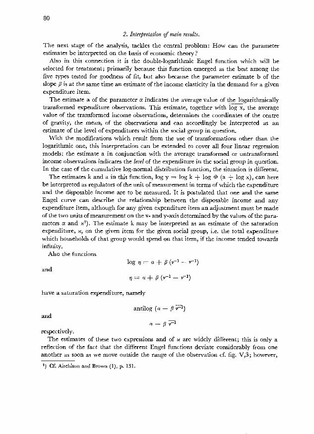
80

2. Interpretation of main results.

The next stage of the analysis, tackles the central problem: How can the parameterestimates be interpreted on the basis of economic theory?

Also in this connection it is the double-logarithmic Engel function which will beselected for treatment; primarily because this function emerged as the best among thefive types tested for goodness of fit, but also because the parameter estimate b of theslope is at the same time an estimate of the income elasticity in the demand for a givenexpenditure item.

The estimate a of the parameter indicates the average value of the logarithmicallytransformed expenditure observations. This estimate, together with log x, the averagevalue of the transformed income observations, determines the coordinates of the centreof gravity, the mean, of the observations and can accordingly be interpreted as anestimate of the level of expenditures within the social group in question.

With the modifications which result from the use of transformations other than thelogarithmic one, this interpretation can be extended to cover all four linear regressionmodels: the estimate a in conjunction with the average transformed or untransformedincome observations indicates the level of the expenditure in the social group in question.In the case of the cumulative log-normal distribution function, the situation is different.

The estimates k and a in this function, log y == log k + log cl (a + log x), can herebe interpreted as regulators of the unit of measurement in terms of which the expenditureand the disposable income are to be measured. It is postulated that one and the sameEngel curve can describe the relationship between the disposable income and anyexpenditure item, although for any given expenditure item an adjustment must be madeof the two units of measurement on the x- and y-axis determined by the values of the para-meters and 7). The estimate k may be interpreted as an estimate of the saturationexpenditure, , on the given item for the given social group, i.e. the total expenditurewhich households of that group would spend on that item, if the income tended towardsinfinity.

Also the functionslog = a + (v' - v1)

and= a + 1 (v' - ir1)

have a saturation expenditure, namely

antilog (a -and

a - fi v1respectively.

The estimates of these two expressions and of are widely different; this is only areflection of the fact that the different Engel functions deviate considerably from oneanother as soon as we move outside the range of the observation cf. fig. V,3; however,7) Cf. Aitchison and Brown (1), p. 131.

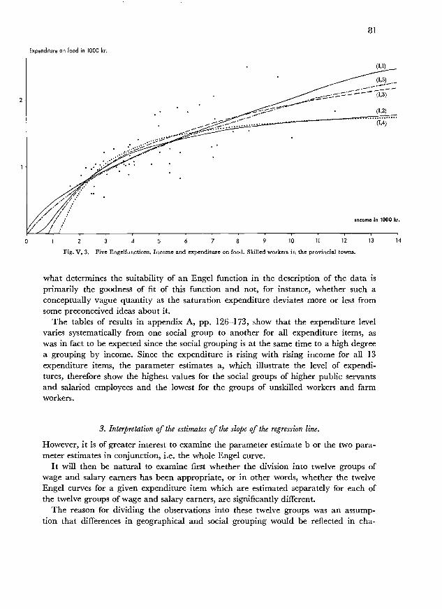
Expenduure on food in 1000 kr.

(1,1)

(")_._--3)-

81

income in 1000 kr.

1 2 3 4 5 6 7 8 9 10 11 12 13 14

Fig. V, 3. Five Engelfunctions. Income and expenditure on food. Skilled workers in the provincial towns.

what determines the suitability of an Engel function in the description of the data isprimarily the goodness of fit of this function and not, for instance, whether such aconceptually vague quantity as the saturation expenditure deviates more or less fromsome preconceived ideas about it.

The tables of results in appendix A, pp. 126-173, show that the expenditure levelvaries systematically from one social group to another for all expenditure items, aswas in fact to be expected since the social grouping is at the same time to a high degreea grouping by income. Since the expenditure is rising with rising income for all 13expenditure items, the parameter estimates a, which illustrate the level of expendi-tures, therefore show the highest values for the social groups of higher public servantsand salaried employees and the lowest for the groups of unskilled workers and farmworkers.

3. Interpretation of the estimates of the slope of the regression line.

However, it is of greater interest to examine the parameter estimate b or the two para-meter estimates in conjunction, i.e. the whole Engel curve.

It will then be natural to examine first whether the division into twelve groups ofwage and salary earners has been appropriate, or in other words, whether the twelveEngel curves for a given expenditure item which are estimated separately for each ofthe twelve groups of wage and salary earners, are significantly different.

The reason for dividing the observations into these twelve groups was an assump-tion that differences in geographical and social grouping would be reflected in cha-

82

racteristic differences in consumption behaviour. To the extent that this geographicaland social grouping is at the same time a grouping by income levels, this will naturallyinfluence the level of the consumption expenditure as shown by the estimate a. Butthe question is whether this grouping is anything more than a grouping by income.May we consider the twelve Engel curves as being generated by the same consumptionprocess, i.e. be considered estimates of the same Engel curve?

This problem can be examined by comparing the twelve regression lines for eachexpenditure item, a comparison which, like the calculation of the parameter estimates,is a standard feature of the regression analysis8).

Such a comparison has been made in the case of the double-logarithmic functionfor all 13 expenditure items.

First, it is examined whether the estimates of the slope b1, b2, ... b12 calculated fora given expenditure item can be considered as estimates of the same "true" slope ,

and if this hypothesis can be upheld, it is examined whether the parallel Engel curvescan be considered as estimates of one single Engel curve. The former test is a test forthe parallelism of the Engel curves, and the latter a test for their identity.

The test for the parallelism of the Engel curves is performed as an F-test, in which avariance calculated on the basis of the variation among the 12 estimated b-values is com-pared with an expression of the inner variance:

s22. 12

Ff2, fi - -i, [f1 = (n - 1) and f2 = 12 - 1]1

12 -s22 = (b - b)2 (log x - log xk)2

11 i

Cf. for instance, A. Hald (8), pp. 579-584.Cf. A. Hald (8), p. 580.

12E(nk-2) s2jogyjx

S2= 112

(nk - 2)i

In these relations log xk and log yk are the coordinates of the mean of the observationsof the k'th group of wage and salary earners; k is the number of observations in thisgroup.

The average slope 1 for a given expenditure item has been calculated as a weightedaverage of the twelve individual slopes 9)

12E (logx - log xk)2

12E E (logx - log xk)21

where

and

83

If the hypothesis is correct (concerning the parallelism of the Engel curves) it will betrue that 15 is normally distributed around fi with the variance

2alogy X= 12

(log xk - log Xk)2i

and the 12 x 13 calculated slopes b have been shown in table V, 10.Table V,9 shows that in 6 out of 13 cases the hypothesis concerning the parallelism

of the Engel curves cannot be rejected, whereas it must be rejected in the 7 remainingcases.

Bearing in mind that the estimate b of the slope in the double-logarithmic Engelcurve is also an estimate of the income elasticity of the expenditure on a given item,it seems to be a reasonable a priori hypothesis that fi varies from the higher to the lowersocial groups because these groups are at different income levels. If y is observed overa sufficiently wide income interval, the income elasticity, i.e. the relative increase inthe expenditure in proportion to a given relative increase in income, must be expectedto be decreasing with increasing income.

Actually it is rather strange that the double logarithmic function, according to whichthe income elasticity is assumed to be constant, should, as far as can be seen from thetests made, turn out to be the "best" of the five types of functions within each of thetwelve social groups, since each social group after all spans an income interval of severalthousand kroner. But if we go further and cover the whole scale from agriculturallabourers and unskilled workers to higher public servants and salaried employees, ahypothesis of constant income elasticity seems to be contrary to all sensible a prioriassumptions.

It is this property of which is utilized in forming the estimate s22.The F-tests appear from table (V,9).

Table V,9. F-test for parallelism of Engel curves.

Dwelling 1.32Fuel and light 4.22Food 3.46Tobacco 2.38Clothing 1.72Footwear 2.40Washing and cleaning 1.06Durables 3.72Personal hygiene 2.89Books, newspapers etc. 1.45Sports, holidays, etc 1.30Transport 6.09Union fees etc 1.89

F.95 1.89

84

Nevertheless, table V,9 shows, as mentioned, that for the six expenditure items:dwelling, clothing, washing and cleaning, books and newspapers, etc., sport and holidays, andfinally uni on fees, etc., such a hypothesis of common slope, i.e. constant income elasticity,cannot be rejected.

It will not be attempted here to explainor rather to explain awaythis phenomenon.As will be remembered, the purpose of the present inquiry has been laid down as anattempt to describe the observations of incomes and expenditures, since an attempt toexplain the consumption behaviour of the households must for the time being be con-sidered unduly ambitious10).

It should be mentioned, however, that the very rough grouping of the almost endlessnumber of goods and services into only 13 items is undoubtedly one of the decisivecauses of the stability found in the income elasticity between social groups. If, instead,sharply defined individual commodities and services had been considered, lounge suitsof a particular quality, flats of a given size and quality, etc. the income elasticity ofdemand for these goods and services would undoubtedly have been falling with risingdisposable income.

However, the six expenditure items with constant income elasticity are not suchheterogenous items in which have been included many different types of goods andservices. The items dwelling, washing and cleaning, clothing, and partly the item sportand holidays, etc. correspond to rather well defined parts of the budget of any household,and it is actually very interesting that the income elasticity for these items is so stableas shown by table V,9. The need for shelter, clothing, for entertainment, etc. naturallymakes itself felt at all income levels, but the interesting thing is that at any place in the in-come scale the same relative increase in the expenditure is produced by a given relative risein income. Not least in the expenditure on the item sport, holidays, etc. does the incomeelasticity seem to be remarkably constant at a very high level around 1.5. Of coursethe goods and services demandedrestaurants, theatres, cinemas, holiday trips, hobbiesand sportvary widely over the different income classes, social groups and age groups,but for all groups there seems to be a very long, still unfulfilled list of demand in thisfield.

For the seven items for which the hypothesis of the parallelism of the regression lineshad to be rejected table V, 10 confirms that as a general rule this is precisely due to thefact that the income elasticity is falling as the income level increases, cf. the items offood, tobacco and footwear. However, this is not the whole explanationindeed, intwo cases the explanation seems to be the opposite, namely that the income elasticityrises with the income, cf. the items offuel and lighting, and transport (incl, expenditure onmotor vehicles), where b in several cases rises as one moves from a lower social groupto a higher one within the same geographical area. In the case of these seven items thereis also another interesting phenomenon which emerges clearly, viz, the significantinfluence of the social grouping on the income elasticity. If, e.g., one takes the largeitem of food, table V, 10 shows that the wage-earning groups in the capital have a con-siderably higher income elasticity in their demand for food than the groups of salaried em-

'°) Cf. E. Jorgensen (12).

85

ployees, 0.69 and 0.70 respectively compared with 0.52 and 0.53. There is also a markeddifference in the level of b in the case offootwear as we move from wage-earners to salariedemployees.

The item of personal hygiene also exhibits significant differences in the b-values forthe two social groups, but here the groups of salaried employees are at the highestlevel. The breakdown into social groups, and particularly the distinction between salariedemployees and manual workers, thus seems to correspond to a real difference in be-haviour in the case of several important items of consumption. The geographical break-down, on the other hand, seems to be justifiable on the basis of existing differences inexpenditure behaviour only as far as the items of dwelling and fuel and lighting are con-cerned.

4. Are the Engel curves for djfferent social groups identical?

For six expenditure items the hypothesis of parallel regression lines for the twelve socialgroups could not be rejected. In these cases it was subsequently examined whether theseparallel curves could be considered as identical (test for identity). This identity test isperformed in two stages; at the first stage it is examined, by means of an ordinary F-testfor linearity, whether the twelve mean points (log xk, ak) can be considered as beingon a straight line-which, of course, they must if the test hypothesis is correct. If this

Table V, 10. Calculated income elasticities for 13 expenditure items for each of 12 groupsof wage and salary earners.

I. Higher public servants and salaried employees. 2. Lower public servants and salaried employees. 3. Skilled workers4. Unskilled workers. 5. Agricultural workers.

The capital Provincial towns Rural districts

2 3 4 2 3 4 2 3 4 5

Dwelling 0.96 0.93 0.87 0.94 0.80 0.86 0.75 0.70 0.84 0.93 0.98 0.96Fuel & light 0.73 0.50 0.40 0.31 0.57 0.44 0.28 0.43 0.55 0.32 0.64 0.76Food 0.52 0.53 0.69 0.70 0.55 0.64 0.60 0.62 0.58 0.65 0.67 0.65Tobacco 0.80 0.84 0.93 1.07 0.76 0.90 1.07 1.17 1.06 0.93 1.28 1.13Clothing 0.89 1.12 1.02 1.05 0.91 1.02 1.10 1.01 1.12 1.02 0.99 1.24Footwear 0.43 0.62 0.50 0.61 0.38 0.57 0.67 0.63 0.71 0.62 0.50 0.49Washing & cleaning 0.80 0.85 0.70 0.81 0.82 0.98 0.90 0.77 0.94 0.88 0.89 0.87Durables excl, vehicles 0.57 0.89 1.21 0.98 1.01 1.04 1.50 1.37 1.10 1.07 0.79 0.85Personal hygiene 0.81 1.00 0.68 0.83 0.73 0.87 0.77 0.97 0.95 0.81 0.87 0.73Books, newspapers etc. 1.02 0.95 0.77 1.05 1.02 1.11 0.86 1.04 0.93 0.86 0.91 1.10Sports, holidays, hobbies 1.39 1.37 1.51 1.46 1.46 1.56 1.68 1.54 1.59 1.61 1.57 1.43Transport incl, own car 0.86 1.09 1.56 1.34 1.68 1.39 1.58 1.62 1.53 1.96 1.66 0.92Union fees, subscriptions etc 0.63 0.66 0.90 1.10 0.76 0.79 0.80 0.91 0.82 0.94 0.94 0.88

3.81 3.75 3.71 3.67 3.75 3.66 3.58 3.53 3.49 3,49 3.47 3.36k5c

86

proves to be the case, it is finally examined, by means of a t-test, whether the slopeF of the line formed by the twelve mean points is identical with the weighted averageof the twelve individual slopes.

It turns out that none of the six expenditure items pass this test for identity. Theitem of sport, holidays, etc. passes the first stage of the test (concerning the linearity of thetwelve mean points), but shows significance for the second stage of the test; the otherfive items show significance already for the linearity test, see fig. V,4a and fig. V,4b,where the twelve mean points have been plotted for the items of books, newspapers,etc. and sport, holidays, etc. together with the twelve individual Engel functions.

Now, what does this result mean? The immediate interpretation is, of course, thatwe are here confronted with the "layer effect" described by Wolcl11) and commentedon page 25 above. The twelve social groups have the same income elasticity for the sixexpenditure items, but there is a difference in the level of the actual expenditure amongthe social groups. This may be due to differences in environment, in upbringing and inhabits of life, or it may be due to differences in the accessibility of the goods in question,for instance, owing to differences in distance from places where the goods are available.Thus restaurants, cinemas and other forms of entertainment are more easily availablein the towns, cf. the instance of this mentioned on page 26.

If this theory of the layer effect holds good, it may be concluded that the sub-division of the material into geographical andparticularlysocial groups correspondsto a real difference in consumption behaviour not only for the seven items with differentincome elasticities, but also for the six items where the twelve social groups could beconsidered as having the same income elasticity; in the case of the latter items the exist-ence of the layer effect should then be the explanation of the difference in the expenditurelevel from social group to social group'2).

If this interpretation of the results is accepted, the conclusion must be that by sub-division of the data into relevant groups it is possible to derive estimates of the income-expenditure relationships which are less biased than those relationships which could bederived for the total sample

If this subdivision had not been undertaken, the income elasticities for the two itemsof books, newspapers, etc. and sport, holidays, etc., to mention two examples, would havebeen considerably higher than the average of the elasticities of the twelve subgroups(viz. 1.28 against 0.98 and 2.00 against 1.50), cf. fig. V,4a and fig. V,4b, on page 87.

5. An important reservation.

As regards this interpretation of the results it is, however, necessary to make an importantreservation. All the results analysed so far are derived from linear regression analyses.In chapter III and IV the assumptions of the inquiry was discussed and it was foundthat this form of analysis was a suitable analytical tool if due regard is paid to problems

Cf. Wold (19), P. 68.Such layer effects may, of course, also be imagined to exist for the seven items for which theEngel curves of the individual social groups are not parallel.

1,4

log y

The capital xThe provincial towns oThe rural districts A

87

3,3 3,4 3,5 3,6 3,7 3,8 og x

Fig. V, 4a. Mean points for the twelve Engel curves for expenditures on books, newspapers etc. For each of the threeparts of the country the capital (X), the provincial towns (0) and the rural districts (e,,) the four Engel curves may be

considered identical. The average Engel curve for whole country deviates significantly.

og y

2,8

2,7

2,6

2,5

2,4

2.3

2,2

2,1

2,0

1,9

The capital x

The provincial towns oThe rural districts 4

3,3 3,4 3,5 3,6 3,7 3,8 log xFig. V, 4b. Mean points for the twelve Engel curves for expenditures on sports, holidays etc. In three cases only oneEngel curve may be considered identical to another one. The average Engel curve for the whole country deviates

significantly.

88

concerning zero observations and variance assumptions. However, it will probably beuseful to point Out that when we choose a given method, we also choose, to some extent,the results. If, for instance, the independent variable of the regression analysis, thedisposable income per person (or transformations hereof), cannot be considered fullyindependent in relation to the dependent variables, there will be bias in the estimates.

Now, considering again fig. V,4b, which shows the Engel curves of the twelve socialgroups with corresponding mean points for the expenditure item of sport, holidays,etc., it may very well be imagined that the line through the twelve mean pointsandnot the twelve single Engel curves deviating systematically from this mean point re-gression linerepresented the "true" relationship between log x and log y. It is worthnoting in this connection that the weighted average of the b for the twelve social groupswas appreciable lower than the estimate of the slope of the regression line through thetwelve mean points in the case of five out of the six expenditure items that had passedthe test for parallelism'3); i.e. displayed the same type of bias as may exist for sports,holidays etc.

On the whole, we are led to conclude that the immediate interpretation of the resultsof the calculations, namely that the subdivision into special groups seems to correspondto real differences in expenditure behaviour is upheld. This is so especially in the caseof the expenditure items where the Engel curves of the social groups showed significantdifferences both in slope and level; but it must be borne in mind that purely technicalfactorshere the choice of the regression technique as analytical toolcan exercisesome influence which would involve modifications of the conclusions drawn.

6. Conclzesions.

If the results for the double-logarithmic Engel function are to be summarized in a singletable, the average income elasticity can be shown for each expenditure item. It is truethat it was found above that these social groups differed systematically as regards theirexpenditures, but this applied primarily to the level of the calculated Engel curves andnot to their slope. In the case of the six items for which the calculated Engel curves couldbe considered parallel the calculation of such averages is natural, and although theelasticities differ significantly for the remaining seven items it is nevertheless charac-teristic that this difference between expenditure items within each social group is morepronounced than the difference between the individual social groups for the sameexpenditure item, so that also here it does make sense to calculate an average b-value.In table V, 11 have been shown the 13 average values for each of the 12 income elasticitiescalculated as a weighted average of the twelve b-values for each item, the weights beingthe sum of the squared deviations from the mean income, cf. above p. 82.

18) The item of union fees, etc. is influenced by the great expenditures of the wage-earning groups onunion fees, so that the line through the mean points of the twelve social groups for this item willhave less slope than the average of the slopes of the twelve individual lines.

Table V, 11. Average income elasticities for 13expenditure items.

I Fuel & light 0.512 Footwear 0.563 Food 0.614 Union fees, subscriptions etc. 0.825 Personal hygiene 0.866 Washing & cleaning 0.867 Dwelling 0.898 Books, newspapers etc. 0.989 Tobacco 0.98

10 Durables excl, vehicles 0.9911 Clothing 1.0412 Transport incl, own car 1.3913 Sports, holoidays, hobbies 1.50

89

In the table the b-values have been arranged by order of magnitude, and it will beseen how the slopes of the Engel curves, i.e. the income elasticities, of the 13 expenditureitems fall into three clearly distinguishable groups: 3 items which could be called neces-sities ranging from 0.51 to 0.61; 8 items which may be labelled neutral goods rangefrom 0,82 to 1.04; and 2 items belonging in the category of luxury goods with 1.39and 1,5014). Reverting to table V,l0, where all b-values have been shown, it will beseen that this ordering by size of average income elasticities comes very close to theordering by size within each of the 12 social groups, so that stability in the incomeelasticity of the main groups of expenditure items seems to be a general feature.

In the discussion of the usefulness of the Engel curve analysis in the description ofthe relationship between x and y, it was found that some expenditure items were not"explained" much more adequately by the inclusion of the disposable income as anexplanatory variablein particular the items of durable goods and transport (incl.transport by own motor vehicle). Now it is found that the estimated parameter valuesfor these items show wide fluctuations of a random nature from social group to socialgroup. The estimate b range from 0.86 to 1.96 for the item of transport and from 0.57to 1.50 for durable goods.

However, the remaining items seem to show such a high degree of stability that thecalculated average income elasticities should be of value also in a wider context, e.g.in the description of the expenditures of the whole population or groups of the populationon these items15).

1) Cf. E. Jørgensen (12).15) Cf. E. Jørgensen (12), where it has been attempted to utilize the results in such a wider context.

AverageExpenditure item income

elasticity

Chapter VI.

FURTHER ANALYSES.THE CONCEPT OF UNIT CONSUMERS, MULTIPLE

REGRESSION ANALYSES, ETC.

VIa. The unit-consumer concept.

The two variables of the Engel function the dependent variable y, i.e. the expenditureon a given item, and the explanatory variable x, i.e. the disposable income, have beendefined (p. 23, chapter III) as expenditure and income per person in the individualhouseholds. The argument in favour of adopting this definition of x and y was, of course,that differences in the size of households (number of persons per household) are re-flected very clearly in the consumption behaviour of the households. When x and yare measured as income and expenditure per person, most of the effects of this sourceof variation in the income-expenditure relationships will be eliminated, particularly inthe case of such main items as food, clothing and footwear depending primarily on thenumber of persons in the household. As far as items such as dwelling, durable goods,sports, holidays and hobbies are concerned, it may be doubtful how much the unex-plained part of the variation in y according to the Engel curve adopted will be reduced.

It is natural to raise the more general question: Is it possible to set up a model for theEngel curve in which x and y are specified in such a way that the effect from differencesnot alone in size of household but also in the type of persons will be eliminated? Or lessambitiously: Can x and y be specified in a way which provides a better approximationto this ideal than the specification used in this analysis (income and expenditure perperson)? This is the approach adopted by Prais and Houthakker in their attempt tocalculate unit-consumer scales separately for each expenditure item, where the scaleindicates, for each type of person, the weight at which the person in question is to beincluded in the specification of x and y for the individual households.

In a household consisting of a man, aged 47, a wife aged 43, a girl of il and a boyof 8, the specification of x and y according to the method adopted in this inquiry wouldsimply consist in dividing the total disposable income of the household and its totalexpenditure on the given commodity group by the number of persons in the household.The unit-consumer scale, as set up by Prais and Houthakker, indicates for each commod-ity or commodity group how these four persons are to be measured to arrive at the divisorwhich gives the desired specification of x and y. The idea is thus that a standard measure is

(VI, 2) y =k,.ni+k2.n2+...+kt.ntf(m)

(VI, 2) is a multiple regression equation, and by ordinary regression analysis k1, k2 . . ,ktmay be determined if y/f (m) is known. It will be seen from the above that the methodis based on ari assumption that the Engel function originally selected is the correct one,also after the observed values have been converted into consumption and income units,and also on an assumption that the effects from the "scale values" of the t types of per-sons enter linearly, since otherwise it will be extremely difficult to solve (VI, 1).

It is easy to point to defects in this approach: the requirement of a priori knowledgeof the "best" type of function and, be it noted, the best one after the consumption unitadjustment, the requirement that the contributions of the individual types of personsto the total income of a given household and total expenditure on a given commoditygroup enter linearly, etc. And it is difficult to see how these defects could be overcome2).But jf such scales could be determined, it would not only be possible to reduce the re-sidual variance, but also to have scales by which it would be possible to answer suchquestions as: How much extra expenditure for a household on a given item wouldbe caused by a ten-year-old boy? etc.

Cf. Houthakker, H. S. and Prais, J. S. (10), p. 133.Cf. Forsyth. (6).

91

introduced, so that for the household mentioned the value on the income scale may be e.g.1.9 units and on the scale for expenditure on food 3.2 units, etc., the unit chosen being theaverage income and average food expenditure, respectively, of one adult male. Prais andHouthakker suggest a method for calculating estimates of such scales'), which may bebriefly described as follows:

By means of the tests the best Engel function is selected. This function is now assumedto give the best description of the relationship between income and expenditure (on agiven commodity in a given population group).

It it is now imagined that all persons in a household are converted into income units(unit e.g. = average income for one married man between 30 and 40 years of age)and consumption units (average consumption for one married man between 30 and 40years of age), the Engel curve chosen wonid then apply to the relationship between in-come per income unit and consumption per consumption unit. If one distinguishes amongt types of persons, the following relationship will apply

(VI, 1) y ' x

k1. ni k01. ni

where Uj is the number of persons in the household of type i, k1 is this type of person'svalue on the consumption unit scale for the given expenditure item, and k01 this type

person's value on the income unit scale. Denotingx bym

E k01. flj

(VI, 1) can be formulated in the following way:

92

Such a tool would be highly relevant in the design of social welfare policy and taxation.But even if it may, on the face of it seem extremely interesting to obtain replies to such

very general questions as the one mentioned above, it seems that questions of this type aretoo general; they cannot be answered satisfactorily since the consumer scale values ofgiven types of persons depend very much on their income level and on the householdtype to which they belong. And if one tries to include these two factors in the consumerscale calculations, these calculations would, for one thing, become enormously compli-cated and for another the result of the calculations would be very difficult to interpret.

These considerations naturally lead up to an attempt to illustrate the influence of thehousehold type in another way. It seems evident that household type and income levelwill have to be taken into account if the objectiveachieving realistic descriptionsisto be fulfilled.

It seems as if this objective could be more satisfactorily fulfilled by calculating income-expenditure relationships separately for the different household types.

In that case one must abandon the idea of a general model describing the observa-tions. The method suggested is more primitive and moderate in its approach, but throughcareful comparison between the Engel curves of different household types, it will prob-ably be possible to achieve a more realistic description. This "method" of treating theinfluence of the household type corresponds completely to the method used in treatingthe residence and social status effect, i.e., separate calculations for each subgroup andcomparison of the results. However, the method presupposes that there is a sufficientnumber of observations for an adequate description of each of the subgroups to be given.In the present study the material has been divided into 12 groups taking into accountdifferences in residence and social status. A further breakdown of each of these 12 groupsinto a large number of subgroups according to household type would not leave a suffi-cient number of observations in each subgroup. It would therefore be necessary toabandon the original grouping and this in turn would necessitate a correction for theobserved differences among the 12 residential and social groups. Such comprehensivecorrection and regrouping have been outside the scope of the present study, and there-fore these calculations have not been made.

In order to get some idea of the influence of the household type, tables VI,la to VI,lnhave been set up. The tables show for the thirteen expenditure items included in the sur-vey and for savings the average expenditure per person for certain income bracketsfor all social groups as a whole, separately for different household types. In the calcu-lation of averages for the whole country of the expenditures of the 12 groups of wageand salary earners the shares of the individual groups in the total population of wageand salary earners have been used as weights. In brackets after each expenditure averagehas been shown the number of observations on the basis of which the average has beencalculated.

In interpreting the tables the weaknesses of such a tabular description must naturallybe borne in mind, confer the remarks on this subject in chapter V, p. 78.

Thus the number of observations in many of the cells of the table is so small that theaverages are subject to so great inaccuracy that their usefulness is rather limited.

Despite the weaknesses of the table, it is still possible to draw some important con-

Table VI, lb. Average expenditure per person on fuel and light in certain income groupsseparately for different types of household.

93

Table VI, la. Average expenditure per person on dwelling in certain income groupsseparately for different types of household.

Type of household

Disposable income per penon

o-1,999

2,000-3,999

4,000-5,999

6,000-7,999

8,000-9,999

10,000-14,999

15,000and above

I Singleman 5(1) 123(5) 200(52) 197(51) 215(68) 270(49) 612(10)2 Single woman 423 (3) 162 (25) 273 (42) 295 (99) 359 (69) 469 (44) 548 (8)3 Couples without

children 235 (4) 289 (84) 347 (234) 340 (172) 384 (99) 456 (45) 530 (2)4 Couples with 1 child 207 (9) 223 (314) 246 (251) 279 (62) 310 (7) 471 (4)5 Coupleswith2children 170 (43) 187 (438) 222 (144) 279 (16) 237 (3) 220 (2)6 Couples with 3 children 145 (58) 171 (146) 190 (34) 185 (3) 214 (1)7 Couples with 4 or more

children 121 (72) 148(40)8 Single man with I or

more children 93 (2) 207 (2) 188 (5) 432 (3) 278 (2) 313 (1)9 Single woman with I

or more children. . 160 (7) 233 (36) 259 (33) 343 (71) 243 (3) 630 (1)10 Other types 132 (18) 188 (88) 281 (49) 325 (12) 508 (5) 634 (1)

Type of household

Disposable income per person

o-1,999

2,000-3,999

4,000-5,999

6,000-7.999

8,000-9,999

10,000-14,999

15,000and above

i Single man 360 (1) 290 509 (6) 560 (51) 820 (69) 950 (49) 1715 (10)2 Single woman 361 (4) 336 (25) 645 (42) 734 (99) 961 (69) 1129 (44) 1410 (8)3 Couples without

children 203 (4) 319 (84) 431 (233) 564 (172) 754 (99) 1042 (45) 1075 (12)4 Couples with 1 child 143 (9) 297 (314) 431 (251) 518 (61) 685 (7) 1176(4)5 Couples with 2 children 172 (43) 261 (438) 386 (144) 534 (16) 737 (3) 305 (2)6 Coupleswith3children 124(58) 234 (146) 356 (34) 428 (3) 278(11)7 Couples with 4 or more

children 116(72) 199(40)8 Single man with 1 or

more children 216 (2) 109 (2) 356 (5) 690 (3) 525 (2) 160 (1)9 Single woman with 1

or more children. . 195 (7) 343 (36) 420 (33) 440 (7) 515 (3) 1364 (1)10 Other types 150 (18) 233 (88) 415 (49) 434 (12) 1076 (5) 918 (1)

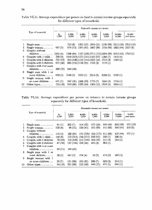
94

Table VI, Ic. Average expenditure per person on food in certain income groups separatelyfor different types of household.

Table VI,ld. Average expenditure per person on tobacco in certain income groupsseparately for different types of household.

Type of household

Disposable income per person

0-1,999

2,000-3,999

4,000-5,999

6,000-7,999

8,000-9,999

10,000-14,999

15,000and above

1 Single man 91(1) 362 (7) 414 (52) 472 (50) 646 (68) 802 (49) 672 (10)2 Single woman 228 (8) 98 (25) 220 (42) 335 (99) 315 (68) 300 (44) 319 (8)3 Couples without

children 116 (4) 188 (84) 272 (234) 405 (172) 411 (99) 452 (44) 357 (1)4 Couples with 1 child 148 (9) 173 (314) 258 (251) 326 (62) 286 (7) 298 (4)5 Coupleswith2 children 78(43) 150 (438) 212 (144) 263 (16) 311 (3) 264 (2)6 Couples with 3 children 87 (58) 137 (146) 206 (34) 405 (3) 364 (1)7 Couples with 4 or more

children 64(71) 144(40)8 Single man with 1 or

more children 28(2) 431 (2) 254 (4) 24(2) 453 (2) 430 (1)9 Single woman with 1

or more children. 18(7) 121 (36) 195 (32) 299 (7) 263 (3) 314 (1)10 Other types 64 (18) 131 (88) 253 (49) 440 (12) 471 (5) 900 (1)

Type of household

Disposable income per person

0-1,999

2,000-3,999

4,000-5,999

6,000-7,999

8,000-9,999

10,000-14,999

15,000and above

i Single man 720(6) 1392(52) 1944(51) 2136(69) 2515(50) 2310(10)2 Single woman 647 (5) 674 (25) 1201 (42) 1687 (99) 1750 (69) 1882 (44) 2027 (8)3 Couples without

children 1056 (4) 1208 (84) 1537 (234)1711 (172)1894 (99) 2053 (45) 1743 (2)4 Couples with I child 799 (9) 1050 (324) 1272 (251)1502 (67) 1588 (7) 1455 (4)5 Couples with 2 children 722 (43) 940(438)1122 (144)1322 (16) 1214(3) 1560(2)6 Couples with 3 children 672(58) 896(146)1156(34) 1518(3) 1174(1)7 Couples with 4 or more

children 599 (72) 849 (40)8 Single man with 1 or

more children 839(2) 1048(2) 1622(5) 2014(3) 2039(2) 2100(1)9 Single woman with 1

or more children. 631 (7) 997 (36) 1368 (33) 1773 (7) 1366 (3) 1724(1)10 Other types 723 (18) 919 (88) 1292 (49) 1585 (12) 1353 (5) 2840 (1)

95

Table VI,le. Average expenditure per person on clothing in certain income groupsseparately for different types of household.

Table VI,lf. Average expenditure per person on footwear in certain income groupsseparately for different types of household.

Type of household

Disposable income per person

0-1,999

2,000-3,999

4,000-5,999

6,000-7,999

8,000-9,999

10,000-14,999

15,000and above

1 Single man 131 (1) 453 (7) 433(52) 530 (51) 657 (69) 1005 (50) 1267 (10)2 Single woman 211 (11) 457 (25) 530 (42) 760 (99) 959 (69) 1152 (44) 1240 (8)3 Couples without

children 274(4) 215 (84) 403 (234) 572 (172) 753 (99) 937 (45) 2489 (2)4 Couples with 1 child 80 (9) 258 (314) 437 (251) 569 (62) 863 (7) 926 (4)

5 Couples with 2 children 136 (43) 259 (438) 464 (144) 827 (16) 592 (3) 336 (2)

6 Couples with 3 children 171 (58) 244 (146) 446 (34) 581 (3) 1064 (1)

7 Couples with 4 or morechildren 124 (72) 297 (40)

8 Single man with 1 ormore children 94(2) 355 (2) 411 (5) 574 (3) 1167 (2) 680 (1)

9 Single woman with 1 ormore children 103 (7) 322 (36) 473 (33) 539 (7) 1052 (3) 636 (1)

10 Other types 123 (18) 251 (88) 359 (49) 578 (12) 551 (5) 971 (1)

Type of household

Disposable income per person

0-1,999

2,000-3,999

4,000-5,999

6,000-7,999

8,000-9,999

10,000-14,999

15,000and above

1 Singleman 35(1) 81(7) 87(52) 118(51) 125(69) 151(50) 144(10)2 Single woman 85 (7) 117 (25) 125 (42) 159 (99) 184 (69) 193 (44) 202 (8)3 Couples without

children 38(4) 48(84) 87(234) 111 (172) 136 (99) 156(45) 259 (2)4 Couples with 1 child. 36 (9) 68 (314) 97 (251) 127 (62) 109 (7) 104(4)5 Coupleswith2 children 43(43) 74(438) 107 (144) 165 (16) 144 (3) 111 (2)6 Couples with 3 children 52 (58) 73 (146) 118 (34) 104 (3) 110 (1)7 Couples with 4 or more

children 41(72) 76 (40)8 Single man with 1 or

more children 52 (2) 94(2) 81(5) 158 (3) 227 (2) 136 (1)9 Single woman with 1

ormorechildren.. 58(7) 104(36) 133(33) 117(7) 167(3) 175(1)10 Other types 41(18) 60(88) 78(49) 115(12) 118(5) 178(1)

96

Table VI, Ig. Average expenditure per person on washing and cleaning in certainincome groups separately for different types of household.

Table VI,lh. Average expenditure per person on durables excl, vehicles in certainincome groups separately for different types of household.

Type of household

Disposable income per person

0-1,999

2,000-3,999

4,000-5,999

6,000-7,999

8,000-9,999

10,000-14,999

15,000and above

1 Single man 53(7) 75(48) 219 (51) 268 (67) 548 (50) 1179 (10)2 Single woman 22 (9) 99 (25) 335 (42) 406 (99) 682 (69) 653 (44) 344 (8)3 Couples without

children 82 (4) 140 (84) 343 (234) 599 (172) 511 (99) 592 (45) 504 (2)4 Couples with 1 child 54(9) 193 (314) 306 (251) 320 (62) 398 (17) 905 (4)5 Couples with 2 children 74(43) 167 (438) 296 (144) 501 (16) 130 (3) 622 (2)6 Couples with 3 children 91(58) 131 (146) 262 (34) 196 (3) 438 (1)7 Couples with 4 or more

children 66 (72) 150 (40)8 Single man with 1 or

more children 32 (2) 80 (2) 138 (5) 244 (3) 502 (2) 222 (i)9 Single woman with 1 or

more children 123 (7) 99 (36) 300 (33) 291 (7) 305 (3) 428 (1)10 Other types 39 (18) 147 (88) 281 (49) 244 (12) 269 (5) 329 (1)

Type of household

Disposable income per person

0-1,999

2,000-3,999

4,000-5,999

6,000-7,999

8,000-9,999

10,000-14,999

15,000and above

1 Single man (1) 107 (7) 150 (52) 180 (51) 213 (69) 297 (48) 247 (10)2 Single woman 24 (6) 38 (25) 92 (42) 147 (99) 165 (69) 199 (44) 207 (8)3 Couples without

children 44(4) 60(84) 88(234) 115 (172) 154 (99) 199 (45) 176 (2)4 Couples with i child 40(9) 63(314) 96(251) 114 (62) 84(7) 103 (4)5 Couples with 2 children 34 (43) 59 (438) 81(144) 120 (16) 99 (3) 81(2)6 Couples with 3 children 36 (58) 53 (146) 79 (34) 41(3) 47 (1)7 Couples with 4 or more

children 32 (72) 49 (40)8 Single man with 1 or

more children 31(2) 86 (2) 133 (5) 123 (3) 135 (2) 65 (1)9 Single woman with i or

more children 59 (7) 74 (35) 101 (33) 124 (7) 95 (3) 256 (1)10 Other types 29 (18) 53 (88) 80 (49) 150 (12) 176 (5) 89 (1)

97

Table VI,li. Average expenditure per person on personal hygiene in certain incomegroups separately for different types of household.

Table VI,lj. Average expenditure per person on books, newspapers, etc. in certainincome groups separately for different types of household.

Type of household

Disposable income per person

0-1,999

2,000-3,999

4,000-5,999

6,000-7,999

8,000-9,999

10,000-14,999

15,000and above

I Single man 113 (1) 105 (7) 129 (52) 159 (51) 162 (69) 206 (48) 219 (16)2 Single woman 99 (6) 146 (25) 185 (42) 302 (99) 296 (69) 320 (44) 413 (8)3 Couples without

children 27(4) 64(84) 117 (234) 170 (172) 214 (99) 243 (45) 142 (2)4 Couples with i child 37(9) 83(314) 124 (251) 155 (62) 121 (7) 169 (4)5 Couples with 2 children 42 (43) 79(438) 122 (144) 164 (16) 244 (3) 120 (2)6 Couples with 3 children 43 (58) 70(146) 114 (34) 75 (3) 173 (1)7 Couples with 4 or more

children 32 (72) 66 (40)8 Single man with 1 or

more children 27 (2) 71(2) 107 (5) 131 (3) 196 (2) 196 (1)9 Single woman with i or

more children 46 (7) 99 (35) 148 (33) 186 (7) 306 (3) 363 (1)10 Othertypes 33(18) 66(88) 120(49) 153(12) 133(5) 207(1)

Type of household

Disposable income per person

Q-1,999

2,000-3,999

4,000-5,999

6,000-7,999

8,000-9,999

10,000-14,999

15,000and above

1 Single man (1) 63 (7) 85 (52) 112 (51) 148 (69) 233 (48) 280 (10)2 Single woman 53 (6) 70 (25) 87 (42) 136 (99) 164 (69) 220 (44) 334 (8)3 Couples without

children 40(4) 55(84) 84(234) 111 (172) 142 (99) 160 (45) 71(2)4 Couples with 1 child 24(9) 46(314) 76(251) 90(62) 120 (7) 97(4)5 Couples with 2 children 25 (43) 45 (438) 71(144) 86 (16) 63 (3) 56 (2)6 Couples with 3 children 24(58) 44 (146) 58 (34) 55 (3) 32 (1)7 Couples with 4 or more

children 18 (72) 44 (40)8 Single man with 1 or

more children 20 (2) 65 (2) 52 (5) 79 (3) 60 (2) 273 (1)9 Single woman with i or

more children 18 (7) 41(35) 81(32) 130 (7) 248 (3) 297 (1)10 Other types 24(18) 40(88) 74(49) 83(12) 119(15) 240(1)

98

Table VI,lk. Average expenditure per person on sports, holidays, hobbies in certainincome groups separately for different types of household.

Table VI,ll. Average expenditure per person on transport incl, own car in certainincome groups separately for different types of household.

Type of household

Disposable income per person

0-1,999

2,000-3,999

4,000.-5,999

6,000-7,999

8,000-9,999

10,000-14,999

15,000and above

I Single man 104(1) 199 (7) 324 (52) 889 (51) 762 (69) 1116 (50) 897 (10)2 Single woman 61(10) 126 (25) 219 (42) 379 (99) 432 (69) 518 (44) 520 (8)3 Couples without

children 42 (4) 105 (84) 227 (234) 429 (172) 750 (99) 1446 (45) 674 (2)4 Couples with 1 child 44 (9) 157 (314) 359 (251) 490 (62) 542 (7) 1609 (4)5 Coupleswith2 children 48 (43) 137 (438) 359 (144) 659 (16) 1359 (3) 3406 (2)6 Couples with 3 children 40 (58) 128 (146) 407 (34) 392 (3) 212 (1)7 Couples with 4 or more

children 54 (72) 206 (40)8 Single man with i or

more children 171 (2) 19 (2) 319 (4) 940 (3) 71(2) 992 (1)9 Single woman with 1 or

more children 50 (7) 86 (36) 144 (33) 297 (7) 336 (3) 264 (1)10 Other types 64 (18) 164 (88) 247 (49) 866 (12) 161 (5) 16 (1)

Type of household

Disposable income per person

0-1,999

2,000-3,999

4,000-5,999

6,000-7,999

8,000-9,999

10,000-14,999

15,000and above

i Single man 851 (1) 305 (7) 574 (52) 730 (51) 1122 (69) 1430 (50) 2774 (10)2 Single women 74(11) 172 (25) 311 (42) 602 (99) 880 (69) 1463 (44) 2061 (8)3 Couples without

children 36 (4) 123 (84) 330 (234) 596 (172) 839 (99) 1288 (45) 1969 (2)4 Couples with i child 52 (9) 189 (314) 360 (251) 741 (62) 1189 (7) 940 (4)5 Couples with 2 children 54(43) 177 (438) 468 (144) 826 (16) 846 (3) 1068 (2)6 Couples with 3 children 62 (58) 165 (146) 397 (34) 760 (3) 1430 (1)7 Couples with 4 or more

children 47 (72) 204 (40)8 Single man with 1 or

more children 33 (2) 285 (2) 367 (4) 399 (3) 547 (2) 1303 (1)9 Single woman with I or

more children 64 (7) 153 (36) 421 (33) 646 (7) 955 (3) 987 (1)10 Other types 66 (18) 169 (88) 352 (49) 705 (12) 571 (5) 1266 (1)

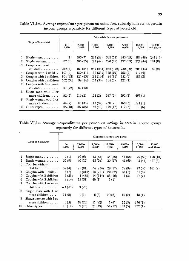
Table VI, ln. Average »expenditure« per person on savings in certain income groupsseparately for different types of household.

99

Table VI, 1m. Average expenditure per person on union fees, subscriptions etc. in certainincome groups separately for different types of household.

Type of household

Disposable income per person

0-1,999

2,000-3,999

4,000-5,999

6,000-7,999

8,000-9,999

10,000-14,999

15,000and above

1 Single man (1) 106 (7) 234 (52) 365 (51) 345 (69) 384 (48) 248 (10)2 Single woman 87 (5) 105 (25) 197 (42) 220 (99) 197 (69) 227 (44) 194 (8)3 Couples without

children 209 (4) 189 (84) 247 (234) 262 (172) 230 (99) 208 (45) 85 (2)4 Couples with 1 child 101 (9) 150 (314) 155 (251) 179 (62) 193 (7) 119 (4)5 Coupleswith2 children 104 (43) 125 (438) 131 (144) 94(16) 132 (3) 187 (2)6 Coupleswith3children 102 (58) 99(146) 117 (34) 164(3) 121 (1)7 Couples with 4 or more

children 67 (72) 87 (40)8 Single man with 1 or

more children 92(2) 114 (2) 134 (2) 197 (3) 292 (2) 467 (1)9 Single woman with 1 or

more children 44(7) 83(35) 111 (32) 238 (7) 168 (3) 124(1)10 Other types 65(18) 107 (88) 146 (49) 179 (12) 112 (5) 78(6)

Type of household

Disposable income per person

0-1,999

2,000-3,999

4,000-5,999

6,000-7,999

8,000-9,999

10,000-14,999

15,000and above

1 Single man 2 (1) 10 (6) 43 (52) 54 (50) 43 (68) 29 (50) 158 (10)2 Single woman 30 (9) 40 (25) 43 (39) 30 (97) 49 (69) 95 (44) 407 (8)3 Couples without

children 52 (4) 25 (84) 34 (234) 29 (172) 72 (99) 77 (45) 181 (2)4 Couples with I child 6 (7) 7 (314) 13 (251) 20 (62) 62 (7) 31(4)5 Couples with2 children 4(38) 4(438) 14 (144) 85(16) 4(3) 47(2)6 Couples with 3 children 2 (14) 12 (34) 40 (3) 1(1)7 Couples with 4 or more

children 1(49) 3 (29)8 Single man with 1 or

11 (2) 1(1) 6(3) 20(2) 10(2) 18(1)more children9 Single woman with 1 or

more children 6 (5) 18 (26) 11(32) 1(6) 25 (3) 170 (1)10 Othertypes 16(10) 9(75) 21(49) 54(12) 197(5) 252(1)

100

clusions from the averages shown. In general it may be said that even if the conversionof all expenditure and income figures from amounts per household into amounts perperson has undoubtedly eliminated also a substantial part of influence of the house-hold type, there still remain systematic effects on the income-expenditure relationshiparising from differences in household type among the observed households. This con-clusion leads to the observation that the existing differences between the residentialand social groups may to some extent be caused by systematic differences in householdtypes between these groups.

Figures VI, 1 and VI,2 show income and expenditure on the items of food and of sports,holidays and hobbies, the most typical necessity item and luxury item, respectively ac-cording to the figures in the tables. For the necessity item the diagram shows that theexpenditure per person for given income per person falls appreciably with the numberof persons (children) in the household. With a given income (per person) the largehouseholds spend a smaller share of their income on food than households with fewpersons. The expenditure items of dwelling and tobacco show the same picture. How-ever, in the case of sports, holidays and hobbies the figure shows an equally appreciableshift in the opposite direction: for a given income per person the expenditure (per per-son) rises with the size of household. The items of clothing and transport present thesame picture, if not quite so markedly.

The conclusion of these results compared with the results of the residential and socialgrouping effect referred to in chapter V above is that future analyses of consumptionsurvey data should presumably place more emphasis on the household type effect and lesson differences in residential and social grouping.

If in the present survey the observations had been divided into only four groups byresidence and social grouping (one group of salary earners and one of wage earners inthe two areas Copenhagen and the rest of Denmark) it should have been possible toundertake Engel curve analyses separately for three household types within each ofthese four groups of wage and salary earners and have the same number of observationsavailable in each Engel curve analysis as in the present survey. Judging from the resultsshown above it seems that such a breakdown of the observations would have givengreater homogeneity in the individual subgroups, and thus presumably more stableEngel curves (i.e. less residual variation) and consequently a more precise descriptionof the observed income-expenditure relationships.

VI.b. Multiple Regression Analyses.

As the main tool in the description of the expenditure behaviour of households of wageand salary earners in this analysis the Engel function has been chosen, in which thedisposable income of the household has been included as the only explanatory variable.A decisive reason for this choice was, of course, that for several purposes it is of interestto know possible expenditure reactions to changes in disposable income.

The object of the analysis has thus been shifted slightly away from the general oneof providing a description of consumption behaviour towards an attempt to show theeffect of income on expenditure. Accordingly it has been attempted to isolate this effect

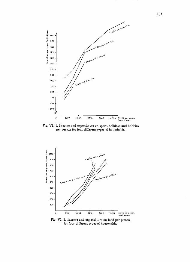
1800

1700

i 1600

1500

140(5

1300

1200

1100

1000

900

800

700

600

500

2000 4000 6000 8000 10,000 Ineorre per personDan(sh Kroner

Fig. VI, 1. Income and expenditure on sport, holidays and hobbiesper person for four different types of households.

10.000 Innorre per perron.Danish Kroner

Fig. VI, 2. Income and expenditure on food per personfor four different types of households.

0 2000 4000 6000 8000

101

1000 -

O 900-o

800

700 -

- 600-

500-

400 -

300 -

200

100 -

102

by careful specification of the two variables and by a subdivision into residential andsocial grouping.

However, if in an attempt to arrive at a good description of the expenditure behaviourof the households one does not wish to be constrained by the considerations that ledto placing the main emphasis on the influence of income and thereby to the preoccu-pation with the Engel curve, it seems natural to try to make the description more com-plete by introducing more explanatory variables in the expenditure functions in addi-tion to disposable income.

Among such variables which may be imagined to influence the expenditures of thehouseholds on the different expenditure items there are a great many about which thebasic material gives no information. There are the prices of the commodities, but alsopast or expected changes in these prices as well as variables reflecting plans or expec-tions in the households.

However, the observations do contain additional information which might be in-cluded in the description of household expenditures on the different commodity groups;presumably the residual variation of y could be reduced thereby. The information re-ferred to concerns expenditures on one or more other commodity groups, the personalwealth of the households, their saving during the survey period and finally the income changesexperienced by the households during the preceding two-year period. Information onthe year of establishment of the households should be valuable as a supplementary variablein the case of certain commodity groups (dwelling, durable goods).

Appendix C gives data on the expenditures of the individual households on all the13 items, so that in the analysis of one expenditure item it would be very simple to includeinformation on the expenditure of the individual households on the other items; theappendix moreover contains information which makes it possible to include all the otherexplanatory variables suggested above.

The present chapter only takes up the expenditure on one of the other commoditygroups for further discussion. This is not because it is thought that this supplementaryinformation necessarily gives the greatest contribution to reducing the residual variationof y, but becauseas a byproduct of the main analysisit is possible to ascertain foreach expenditure item y1 the expenditure item yt which will give the greatest effect ifadded as supplementary explanatory variable.

The more comprehensive analysis introducing one or more of the data shown in theappendix (income changes, personal wealth, etc.) with a view to providing a moreadequate description or explanation of the expenditure behaviour of the households,therefore still remains. In this connection it should be mentioned that in a separate studyof the saving pattern of households it was found that particularly income changes seemedto have great effect3). Households with rising incomes recorded considerably highersavings than households who had experienced a fall in income. Moreover, differencesin personal wealth were reflected in significant differences in saving (for given incomelevel), households whose personal wealth was around zero saving less than householdswith considerable psoitive or negative wealth4). It is, perhaps, not unreasonable toexpect that these variables would also have an effect in the explanation of the expendi-ture on some of the commodity groups (particularly durable goods).

103

In choosing an expenditure item, y, as supplementary explanatory variable for theexpenditure yj, the criterion for selecting Yh must be some expression of the correlationbetween yj and y. However, this expression must naturally be adjusted for the in-fluence of income, on both variables. The problem is this: If a household with a givenincome, residence, social grouping, household type, etc., has a higher expenditure onitem i than expected according to the "best" Engel function, can this be ascribed to anyappreciable extent to this household's expenditure on item h?

It is here necessary to point out that every expenditure item yj can be described or"explained" exhaustively by means of the income and all other m - I expenditureitems including savings on the basis of the budget relation

(VI, 3) = i1 y

It is obvious that a given household's expenditure on commodity group No. i is uni-quely determined if the disposable income and all other uses of that income are in-cluded in the explanation. There will then be so many constraints on the variablesthat there simply are no more degrees of freedom left. According to the budget relation(VI, 3) the following identity exists

(VI, 4) yj=x h'1

Thepositive or negativecorrelation between the residuals in the relations de-scribing household expenditures on items i and h will determine whether it will beuseful to include yh in the description of yj. It is evident that such a correlation willbe most marked in the case of commodities which are close substitutes or complementsin the consumption of the households. Abnormally high consumption of butter willthus, probably, occur at the same time as abnormally low consumption of margarine,high values for expenditure on petrol will often occur together with high values forexpenditure on purchases of motor cars, etc.

In the breakdown of expenditure items which has been undertaken in the presentanalysis it has been attempted to place commodities which, in the opinion of thehousehold are closely related to one another in the same group, cf. chapter IV, p. 38;the 13 expenditure items represent as far as possible 13 "unrelated" commodity cate-gories, and the mentionedpositive or negativecorrelation cannot therefore be ex-pected to have any high value.

If now the best of the Engel functions studied is taken and for each of the expenditureitems in question are calculated the residuals for the individual households from theexpected expenditure, a table of the correlation between these deviations for each item canbe set up. Such a correlation table for the group of skilled workers in the capital has beengiven in table VI,2. Inthe appendix will be found such tables for all twelve groups of wage

Opsparing i lønmodtagerhusstandene 1955, Statistiske Undersøgelser, No. 3, Copenhagen 1960, p. 31.Same as above, pp. 31-32.

Table VI,2. Correlation between each two of thirteen expenditure items.

Skilled workers. The Capital.

1. Dwelling. 2. Fuel and light. 3. Food. 4. Tobacco. 5. Clothing. 6. Footwear. 7. Washing and cleaning. 8. Durable goods. 9. Personal hygiene. 10. Books, news-papers etc. 11. Sports, holidays, etc. 12. Transportation. 13. Union fees and subscriptions.

1 2 3 4 5 6 7 8 9 10 11 12 13

- 0.369 -0.117 0.003 -0.324 -0.283 -0.046 0.054 -0.047 0.155 0.025 0.017 0.1622 - - 0.110 -0.057 -0.185 -0.146 -0.126 0.015 -0.038 0.205 -0.066 -0.124 0.2253 - - - -0.017 -0.193 -0.037 0.267 -0.165 0.065 0.079 0.048 -0.340 0.1974 - - - - -0.127 -0.089 0.244 0.085 0.102 0.034 0.171 -0.185 -0.0315 - - - - - 0.480 -0.176 0.112 0.265 0.061 0.110 0.010 -0.2076 - - - - - - -0.132 0.056 0.120 -0.077 0.074 -0.077 -0.1227 - - - - - - - -0.055 0.018 0.099 0.204 -0.035 0.0868 - - - - - - - - 0.076 0.152 0.109 -0.182 -0.0399 - - - - - - - - - 0.173 0.116 0.018 -0.055

10 - - - - - - - - - - 0.165 -0.110 0.064il - - - - - - - - - - - -0.219 -0.22712 - - - - - - - - - - - --0.09713 - - - - - - - - - - - - -

Unskilled workers. The Capital.

1 2 3 4 5 6 7 8 9 10 11 12 13

1 - 0.336 -0.097 0.024 0.161 0.122 0.151 0.067 0.169 0.074 0.034 -0.167 -0.0162 - - -0.166 -0.034 -0.171 -0.123 -0.073 0.133 0.079 -0.031 -0.049 0.020 0.1273 - - - 0.133 0.025 -0.086 0.275 -0.143 0.014 0.114 0.049 -0.032 0.1864 - - - - -0.100 -0.030 0.186 -0.104 0.025 0.069 0.024 0.041 0.1295 - - - - - 0.532 0.172 0.196 0.338 0.126 0.182 -0.187 0.0346 - - - - - - 0.265 0.099 0.300 0.053 0.092 -0.032 -0.0667 - - - - - - - -0.034 0.121 0.180 -0.049 -0.026 -0.0298 - - - - - - - - 0.111 -0.023 -0.053 -0.161 0.0409 - - - - - - - - - 0.110 0.083 -0.012 0.114

10 - - - - - - - - - - 0.102 -0.171 0.19011 - - - - - - - - - - - -0.164 0.18612 - - - - - - - - - - - ---0.01613 - - - - - - - - - - - - -

andN

SSDh= E(Yh,Jyh,J)2

r= S P D,, h

s s D1. S S Db

N N

where E (Y1, j - y', j) E (Yh, j - yb, j)N

j jSPDI,b=E(Y,,jyj,j)(Yh,jyb,J)N

and2

IN t

N (E(Yj,j_yj,j))/

N'N 2

(E (Yh, j - Yb,'jN

105

and salary earners, cf. appendix B, p. 174. Table VI,2 shows for each of the 13 expendi-ture items the correlation between the deviations of the individual households from theexpected expenditure on this item and the deviation from the expected expenditure oneach of the other 12 expenditure itemswhere the expected expenditure has been cal-culated according to the double logarithmic Engel function.

An estimate of the correlation between the deviations of the observed values of twoexpenditure items from the calculated values according to the double logarithmic func-tion should be based on the logarithmically transformed expenditures. However, since,i.a. for technical reasons, correlations had to be computed on the basis of the individualhouseholds and not on the basis of the deviations of expenditures of groups of households,the zero observation problem again arose, cf. p. 36 above, and it was therefore decidedto base the calculations on the deviations of the untransformed, observed expendituresfrom the antilogarithm of the calculated value f (x) = a + b (log x - log x). Forexpenditure items No. i and h the estimate of the correlation coefficient, r, is accordinglyobtained in the following way

where Y1, j = antilog f1 (xj) and Yb, j = antilog fh (xj)

Since it is expenditures rather than logarithms of expenditures which are used, theexpenditure deviations will, in the case of the high income brackets, be included withtoo much weight a consequence of which is a certain bias. The primary aim in computingthe correlations has been to find the sets of expenditure items which were "closest" or"farthest", and not to measure how close or how far. In other words the computationsoffer a qualitative rather than a quantitative impression; it has not, accordingly, beenattempted to introduce any correction for the bias in the correlation coefficients andthe tables must therefore be read with this reservation in mind.

It must also be borne in mind that the budget relation (VI, 3) brings about a slightnegative correlation between the expenditure residuals in the equations explaining the in-

106

Table VI,3. The biggest positive and negative correlationcoefficiertt

dividual items. A household with au expenditure considerably above the expected ex-penditure ou au item which weighs heavily in the budget must necessarily display ne-gative deviations from the expected expenditure on one or more of the other items.However, this cannot be seen from the correlation tables, partly because the incomeconcept used, disposable income, is not precisely equal to the sum of the 13 expenditureitems studied, as some small items (domestic help, gifts and charity, etc.) are left out,which is also the case for the part of the disposable income used for saving, and partlybecause of the above-mentioned bias in the correlation estimates.

Only very few of these correlation estimates exceed a level as moderate as 0.5, whichis some sort of a confirmation of the impression that the commodity classification hasbeen reasonable, cf. above. Even if very high correlation values do not occur, there isstill, in the case of some items, a considerable correlation between the deviations of thehouseholds from the expected expenditure behaviour. Consequently the description ofthe expenditure behaviour of the households with regard to these commodity groupswill evidently become more satisfactory (resulting in a lower residual variance of the

Expenditure item

Group of wage

2 3 4

1 Dwelling positive 2 0.309 2 0.395 2 0.369 2 0.336negative 13 -0.100 4 -0.055 5 -0.324 12 -0.167

2 Fuel and light positive 1 0.309 1 0.395 1 0.369 1 0.336negative 11-0.385 11 -0.144 5-0.185 5-0.171

3 Food positive 7 0.365 4 0.262 7 0.267 7 0.275negative 8 -0.045 12 -0.261 12 -0.340 2 -0.166

4 Tobacco positive 3 0.288 3 0.262 7 0.244 7 0.186negative 13 -0.156 6 -0.064 12 -0.185 8 -0.104

5 Clothing positive 6 0.578 6 0.469 6 0.480 5 0.532negative 2 -0.240 2 -0.125 1 -0.324 12 -0.187

6 Footwear positive 5 0.578 5 0.469 5 0.480 5 0.532negative 12 -0.112 2 -0.075 1 -0.283 2 -0.132

7 Washing and cleaning . positive 3 0.365 9 0.236 3 0.267 3 0.275negative 12- 0.027 8 -0.043 5 -0.176 2 -0.073

8 Durable goods positive 1 0.176 6 0.148 10 0.152 5 0.196negative 10 -0.139 12 -0.054 12 -0.182 12 -0.161

9 Personal hygiene positive 5 0.485 5 0.365 5 0.265 5 0.338negative 2 -0.145 2 -0.139 13 -0.055 12 -0.012

10 Books, newspapers etc. positive 9 0.381 13 0.347 2 0.205 13 0.190negative 2-0.181 12 -0.116 12 -0.110 12 -0.171

11 Sports, holidays etc positive 5 0.359 4 0.102 7 0.204 13 0.186negative 2 -0.385 10-0.116 13 -0.227 12 -0.167

12 Transportation positive 13 0.065 4 0.102 9 0.018 4 0.041negative 6-0.114 10-0.116 3-0.340 5-0.187

13 Union fees and subscriptions positive 11 0.141 10 0.347 2 0.225 10 0.190negative 2 -0.156 6-0.006 11 -0.227 6-0.066

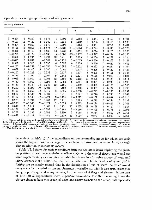
separately for each group of wage and salary earners.

and salary earners*)

*) 1. Higher public servants and s3. Skilled workers, the Capital; 4towns; 6. Lower public servantsworkers, provincical towns; 9. Lil. Unskilled workers, rural districts

107

alaried employees, the Capital; 2. Lower public servants and salaried employees, the Capital;Unskilled workers, the Capital; 5. Higher public servants and salaried employees, the provincical

and salaried employees, provincical towns; 7. Skilled workers, provincical towns; 8. Unskilledower public servants and salaried employees, rural districts; 10. Skilled workers, rural districts

12. Farm workers, rural districts.

dependent variable y) if the expenditure on the commodity group for which the tableshows the highest positive or negative correlation is introduced as an explanatory vari-able in addition to disposable income.

Table VI, 3 shows for each expenditure item the two other items displaying the great-est positive or negative correlation coefficient. Only in the case of three items would thesame supplementary determining variable be chosen in all twelve groups of wage andsalary earners if this table were used as the criterion. The items of dwelling and fuel &lighting are so closely related that in the description of one of them the other wouldeverywhere be included as the supplementary variable yi. This is also true, except forone group of wage and salary earners, for the items of clothing and footwear. In the caseof both sets of expenditures there is positive correlation. For the remaining items thepicture changes from one group of wage and salary earners to the other, and especially

5 6 7 8 9 10 11 12

2 0.294 2 0.250 2 0.278 2 0.292 2 0.183 2 0.341 2 0.191 2 0.49112 -0.122 11 -0.160 4-0.302 11 -0.335 8 -0.199 6 -0.205 3-0.174 11 -0.233

1 0.294 1 0.250 1 0.278 1 0.292 1 0.183 1 0.341 10 0.296 1 0.4915-0.192 9 -0.252 11 -0.274 12 -0.288 11 -0.263 11 -0.224 11-0.447 11-0.2282 0.338 13 0.159 13 0.288 13 0.260 11 0.174 13 0.214 7 0.165 10 0.2205 -0.235 8-0.132 8 -0.236 5 -0.388 13 -0.172 8 -0.327 1 -0.174 1 -0.1909 0.368 7 0.204 7 0.293 10 0.211 11 0.315 2 0.254 9 0.228 7 0.2208 -0.095 8 -0.094 1 -0.302 8 -0.135 2 -0.099 8 -0.234 2 -0.253 8-0.1249 0.507 6 0.510 6 0.596 6 0.590 6 0.428 6 0.496 6 0.447 6 0.4583 -0.235 2 -0.252 12 -0.396 3 -0.388 2 -0.222 8 -0.292 13 -0.230 12 -0.1955 0.469 5 0.510 5 0.596 5 0.590 5 0.428 5 0.496 5 0.447 5 0.4583 -0.200 2 -0.223 12 -0.336 3 -0.327 2 -0.227 1 -0.205 3 -0.101 2 -0.146

13 0.371 4 0.204 11 0.467 9 0.482 9 0.291 5 0.429 13 0.210 11 0.33312 -0.093 8 -0.044 2 -0.202 12 -0.196 11 -0.152 12 -0.305 1 -0.125 8 -0.2145 0.130 9 0.052 5 0.191 6 0.088 5 0.251 11 0.054 9 0.240 9 0.290

11 -0.130 3 -0.132 13 -0.242 12 -0.191 1 -0.199 3 -0.327 13 -0.175 11 -0.2455 0.507 6 0.397 10 0.309 7 0.482 6 0.360 7 0.384 6 0.402 5 0.2992-0.182 2 -0.252 12 -0.045 3 -0.326 2 -0.248 8 -0.229 2 -0.146 3 -0.153

11 0.282 11 0.182 9 0.309 4 0.211 7 0.171 9 0.276 2 0.296 7 0.26212 -0.162 1 -0.130 12 -0.223 8 -0.174 1 -0.112 8 -0.188 11-0.091 8-0.1159 0.323 4 0.191 7 0.467 12 0.411 4 0.315 6 0.216 6 0.254 7 0.3333 -0.206 2 -0.165 2 -0.274 1 -0.335 2 -0.263 2 -0.224 2 -0.447 8 -0.242

13 0.049 7 0.014 1 0.062 11 0.411 10 0.130 11 0.136 1 0.122 7 0.32211 -0.182 2 -0.167 5 -0.396 2 -0.288 2 -0.186 7 -0.305 3 -0.173 5-0.1957 0.371 3 0.159 3 0.288 3 0.260 7 0.110 3 0.314 7 0.210 10 0.2428 -0.072 12 -0.139 8-0.242 9 -0.200 11 -0.180 8-0.270 5 -0.230 5 -0.162

108

Table VI,4. The highest and lowest values of the correlationcoefficient of deviations,separately for each social group

S) I. Dwelling. 2. Fuel and light. 3. Food. 4. Tobacco. 5. Clothing 6. Footwear. 7. Washing and cleaning.8. Durables excl, own car, 9. Personal hygiene. 10. Books, newspapers etc.. I I - Sports, holidays, hobbies, etc. 12. Trans-port, incl, own car. 13. Union fees, subscriptions etc.

in the case of the negatively correlated items such typically interrelated expendituresets are lacking.

Table VI,4 gives the five highest coefficients of correlation of each category (positiveand negative) for each of the twelve groups of wage and salary earners. Also here especi-

Social groups

Highest Lowest

Expendituregroup*) Coefficients Expenditure

group*) Coefficient

1 5-6 0.578 2-11 -0.385Higher public servants and salaried 5-9 0.485 2-5 -0.240employees, the Capital 6-9 0.432 2-10 -0.181

9-10 0.381 2-13 -0.15610-11 0.378 4-13 -0.156

2 5-6 0.469 2-11 -0.144Lower public servants and salaried 1-2 0.395 2-9 -0.139employees, the Capital 6-9 0.370 2-5 -0.125

5-9 0.365 10-12 -0.11610-13 0.347 2-6 -0.075

3 5-6 0.480 3-12 -0.340Skilled workers, the Capital 1-2 0.369 1-5 -0.324

3-7 0.267 l-6 -0.2835-9 0.265 11-13 -0.2274-7 0.244 11-12 -0.219

4 5-6 0.532 5-12 -0.187Unskilled workers, the Capital 5-9 0.338 5-2 -0.171

1-2 0.336 10-12 -0.1716-9 0.300 1-12 -0.1673-7 0.275 2-3 -0.167

5 5-9 0.507 3-5 -0.235Higher public servants and salaried 5-6 0.469 3-11 -0.206

employees, provincial towns 6-9 0.423 3-6 -0.2007-13 0.371 2-5 -0.1924-9 0.368 2-9 -0.182

6 5-6 0.510 2-5 -0.252Lower public servants and salaried 6-9 0.397 2-9 -0.252employees, provincial towns 5-9 0.390 2-6 -0.223

1-2 0.250 2-12 -0.1674-7 0.204 2-11 -0.165

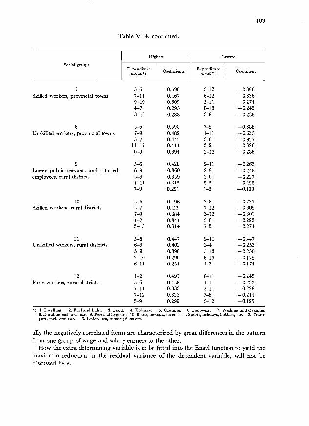
Social groups

7Skilled workers, provincial towns

8Unskilled workers, provincial towns

10Skilled workers, rural districts

11

Unskilled workers, rural districts

12

Farm workers, rural districts

Table VI,4. continued.

Expendituregroup*)

Highest

Coefficients Expendituregroup')

Lowest

Coefficient

5-6 0.596 5-12 -0.3967-11 0.467 6-12 -0.3369-10 0.309 2-11 -0.2744-7 0.293 8-13 -0.2423-13 0.288 3-8 -0.236

5-6 0.590 3-5 -0.3887-9 0.482 1-11 -0.3355-7 0.445 3-6 -0.327

11-12 0.411 3-9 -0.3266-9 0.394 2-12 -0.288

9 5-6 0.428 2-11 -0.263Lower public servants and salaried 6-9 0.360 2-9 -0.248employees, rural districts 5-9 0.359 2-6 -0.227

4-11 0.315 2-5 -0.2227-9 0.291 1-8 -0.199

5-6 0.496 3-8 -0.2 375-7 0.429 7-12 -0.3057-9 0.384 3-12 -0.3011-2 0.341 5-8 -0.2923-13 0.314 7-8 -0.274

5-6 0.447 2-11 -0.4476-9 0.402 2-4 -0.2535-9 0.398 5-13 -0.2302-10 0.296 8-13 -0.1756-11 0.254 1-3 -0.174

1-2 0.491 8-11 -0.2455-6 0.458 1-11 -0.2337-11 0.333 2-11 -0.2287-12 0.322 7-8 -0.2145-9 0.299 5-12 -0.195

109

*) 1. Dwelling. 2. Fuel and light. 3. Food. 4. Tobacco. 5. Clothing. 6. Footwear. 7. Washing and cleaning.8. Durables excl, own car. 9. Personal hygiene. 10. Books, newspapers etc. il. Sports, holidays, hobbies, etc. 12. Trans-port, incl, own car. 13. Union fees, subscriptions etc.

ally the negatively correlated items are characterized by great differences in the patternfrom one group of wage and salary earners to the other.

How the extra determining variable is to be fitted into the Engel function to yield themaximum reduction in the residual variance of the dependent variable, will not bediscussed here.

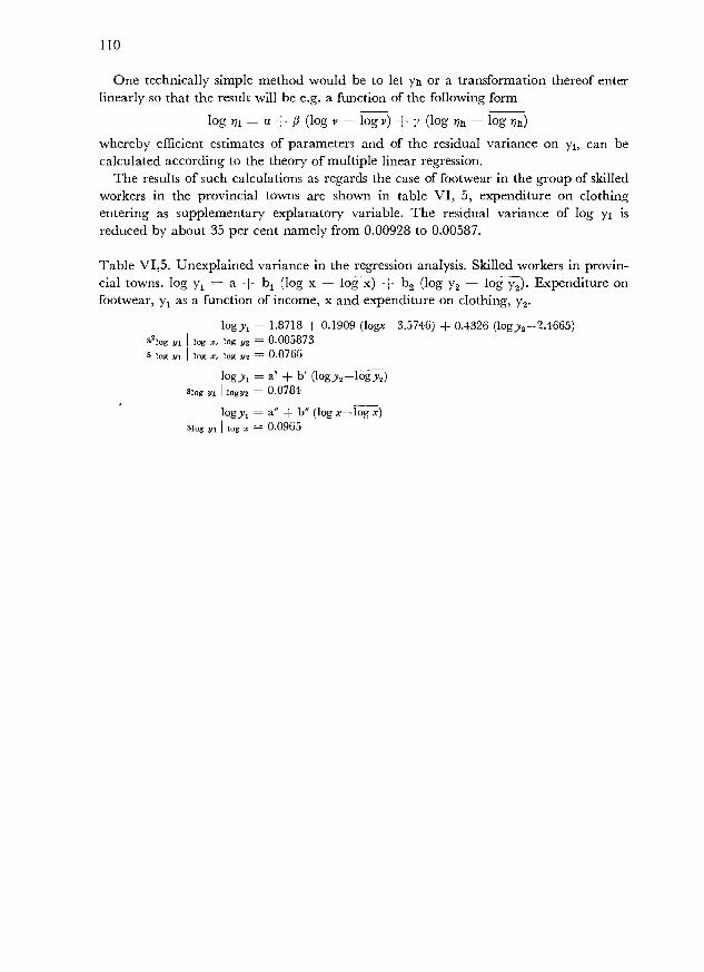
110

One technically simple method would be to let y or a transformation thereof enterlinearly so that the result will be e.g. a function of the following form

log j = a + fi (log y - log r) + (log h - log 17h)

whereby efficient estimates of parameters and of the residual variance on y, can becalculated according to the theory of multiple linear regression.

The results of such calculations as regards the case of footwear in the group of skilledworkers in the provincial towns are shown in table VI, 5, expenditure on clothingentering as supplementary explanatory variable. The residual variance of log yj isreduced by about 35 per cent namely from 0.00928 to 0.00587.

Table VI,5. Unexplained variance in the regression analysis. Skilled workers in provin-cial towns, log y1 = a + b1 (log x - log x) + b2 (log y2 - log y2). Expenditure onfootwear, y1 as a function of income, x and expenditure on clothing, y2.

logy1 = 1.8718 + 0.1909 (Iogx-3.5746) + 0.4326 (logy2-2.4665)S2log i log z, log 112 = 0.005873S log iii log z, log Y2 = 0.0766

logy1 = a' + b' (logy2logy2)Slog 111 logyz = 0.0784

logy1 = a" + b" (log xlog x)Slog yi log z = 0.0965

DANSK RESUMÉ

Undersøgelsen af danske lønmodtagerhusstandes indkomst-, forbrugs- og opsparingsforholdfor året 1955, som gennemførtes i begyndelsen af året 1956, er den største og mestdetaillerede af de forbrugsundersøgelser, Det statistiske Departement har foretaget, sidenman i 1897 påbegyndte denne art af undersøgelser. Forbrugsundersøgelsernes primæreformål var oprindelig at fremskaffe oplysning om »Livsvilkår i de forskellige samfundslag,derunder ernærings- og forbrugsforhold,1) men efter at pristalsreguleringen af lønningerog ydelser og tilskud af forskellig art vandt stærkt frem, har de foretagne forbrugsunder-søgelser her som i mange andre vesteuropæiske lande i første række skullet tjene som red-skab til opstilling af vægte ved prisindeksberegningerne. I de seneste år synes imidlertiddet alment beskrivende, som var det primære sigte med de første forbrugsundersøgelser,atter at komme i første række. Dette skyldes bl.a., at man har erkendt, at det grund-materiale, som tilvejebringes ved en omhyggelig planlagt og udført forbrugsundersøgelse- i denne forbindelse må de senere års betydelige fremskridt indenfor undersøgelsesteknik-ken haves i erindring - rummer oplysninger om væsentlige økonomiske sammenhænge isærvedrørende anvendelsen af den indtjente indkomst, der ikke, eller kun mangelfuldt,kan belyses ad anden vej.2)

Forbrugsundersøgelsen for året 1955 har da også været genstand for en mere omfat-tende bearbejdelse end nogen af de foregående undersøgelser.

En almindelig oversigt over 1955-undersøgelsen, dens tilrettelæggelse og dens hoved-resultater er givet i Statistiske Efterretninger i l957.) Fødevareforbruget blev særskiltbehandlet i en artikel i Statistiske Efterretninger i l958.) De indhentede oplysningervedrørende lønmodtagerhusstandenes opsparings- og formueforhold blev gjort til gen-stand for en særskilt analyse, hvis resultater meddeltes i et hæfte i serien Statistiske Under-søgelser i l96O.) I samme serie behandledes de indhentede oplysninger om lønindkom-sternes fordeling og sammensætning6).

Hovedparten af de indhentede oplysninger fra de adspurgte lønmodtagerhusstandevedrørte disses husstandes forbrugsudgifter i året 1955, og man besluttede derfor atunderkaste lønmodtagernes forbrugsadfærd en mere indgående analyse. Det er resul-taterne fra denne analyse, der indeholdes i nærværende publikation.

1) Lov om Statens statistiske Bureau 1895.2)Jfr. I. L. 0. (11).

Statistiske Efterretninger 1957, nr. 83.Statistiske Efterretninger 1958, nr. 46.Opsparing i lønmodtagerhusstandene 1955, Statistiske Undersøgelser nr. 3, Kbh. 1960.Lønmodtagerindkomster, Fordeling og sammensætning, Statistiske Undersøgelser nr. 6, Kbh. 1962.

112

2. Analysens hovedresultater.

Analysen tilsigtede at give en præcis beskrivelse af sammenhængen mellem de danskelønmodtagerhusstandes disponible indkomst og udgiften til nogle væsentlige udgifts-poster i året 1955. Denne sammenhæng mellem disponibel indkomst og udgiften tilgivne udgiftsposter er utvivlsomt af væsentlig betydning, hvis man vil prove at forklareforskelle i forbrugsadfærd fra den ene husstand til den anden, selvom naturligvis mangeandre forhold spiller ind såsom husstandstype, bopæls- og socialgruppering m.v. Ind-komst-udgiftsrelationen er imidlertid tillige af væsentlig betydning, hvis man vil for-søge at foretage skøn over forbrugets sandsynlige udvikling ved givne, alternative ind-komstforskydninger, hvad enten dette nu drejer sig om den enkelte husstand eller hus-standsgruppe, eller det drejer sig om alle husstande under eet.7)

Hovedvægten i analysen blev derfor lagt på udledning af de indkomst-udgiftsrelationer,som ifølge det foreliggende grundmateriale gav den bedste beskrivelse af sammenhængen.De nævnte indkomst-udgiftsrelationer går ofte under betegnelsen Engelfunktioner efterden tyske økonom og statistiker, Ernst Engel, og det konkrete analysearbejde har be-stået i at beregne skøn over parametrene i fem på forhånd udvalgte funktionstyper ogderefter ved et antal test at sammenligne disse funktionstyper for at finde frem til denfor hver udgiftspost bedst egnede Engelkurve.

For at eliminere de væsentligste forstyrrende påvirkninger hidrorende fra forskelle ihusstandsstørrelse i de undersøgte husstande omregnedes alle udgifts- og indkomstbeløbfor hver af de 3100 husstande til beløb pr. person.

Engel funktionens uafhængigt variable fastlagdes som disponibel indkomst (samtligekontantindtægter minus betalte personlige skatter) pr. person, og der blev udledt Engel-funktioner for følgende 13 udgiftsposter, der tilsammen udgør 85 pct. af totalforbrugetfor samtlige lønmodtagerhusstande.

Bolig.Brændsel og belysning.Fødevarer (incl, regelmæssig fortæring ude og ø1, vin og spiritus indenfor detsædvanlige husholdningsforbrug).Tobak.Beklædning.Fodtøj.Vask og rengøring.Varige goder (excl. motorkøretøjer).Personlig pleje.Bøger, aviser m.v.Sport, ferie, fritid m.v. (incl. restaurationsbesøg, teater, biograf og øl, vin ogspiritus uden for det sædvanlige husholdningsforbrug).Transport (incl. motorkøretøjer).Kontingent og forsikringer m.v. (excl, livs- og pensionsforsikringer).

Beregningerne udførtes særskilt for 12 lønmodtagergrupper, nemlig 4 socialgrupperindenfor hver af 3 landsdele, jfr. resultattabellen i bilag A. De 5 funktionstyper, hvis7) Jfr. Erling Jorgensen (12), side 54-61.

113

parametre man dannede skøn over, var følgende, hvor y betegner den disponible indkomstog s udgiften til en given udgiftspost:

(1) logi = a+ fi(logv logy)

(2)log=a+fi( -i = a + fi (log y - log )

i=a+fi(! -log i = log + log [ (a + log y)]

Væsentlige dele af analyserapporten behandler estimationsproblemer, således atman kan sige, at udredningen af analysemetoderne var et andet hovedformål ved analyse-arbejdet ved siden af selve beregningen af analyseresultaterne.

De foretagne testberegninger viste næsten samstemmende, at funktionstype (1), dendobbeltlogaritmiske funktion, for samtlige 13 udgiftsposter gav den bedste fremstillingaf Engelrelationen. Dette resultat er i en vis forstand overraskende, fordi det indebærer,at indkomstelasticiteten i de pågældende husstandes efterspørgsel efter de 13 udgiftsposterer konstant (for given socialgruppe, idet beregningerne som nævnt er udført særki1t for12 lønmodtagergrupper) og altså uafhængig af indkomstniveauet. Dette følger af, atindkomstelasticiteten er identisk med parameteren i den dobbeltlogaritmiske Engel-funktion. Man måtte vel på forhånd vente, at varegrupper, der i de højeste indkomst-grupper betragtes som nødvendighedsvarer (lav indkornstelasticitet), i de lavere ind-komstgrupper ville gå over til at blive betragtet som luksusvarer (høj indkomstelasticitet).Imidlertid viser det sig8), at der er en bemærkelsesværdig stabilitet til stede, også nårvi går fra lønmodtagergruppe til lønmodtagergruppe for så vidt angår det nævnteparameterskøn over fi, skønnet over indkomstelasticiteten. For 6 udgiftsposters vedkom-mende kan en hypotese om konstant indkomstelasticitet alle 12 lønmodtagergrupperigennem opretholdes, og for de resterende 7 posters vedkommende er afvigelserne omendstatistisk signifikante dog ikke særligt store. Konstateringen af denne stabilitet i lønmod-tagerhusstandenes indkomstelasticitet i udgiften til de væsentligste udgiftsposter er et alde mest iøjnefaldende resultater af analysearbejdet9).

Denne stabilitet gør det forsvarligt at beregne gennemsnit af de 12 lønmodtagergrup-pers indkomstelasticiteter for hver de 13 udgiftsposter. Disse gennemsnitselasticiteter ervist i nedenstående oversigt, hvor udgiftsposterne er ordnet efter gennemsnitsindkomst-elasticitetens størrelse.

Man ser umiddelbart af denne tabel, at de beregnede gennemsnitselasticiteter falderi tre klart afgrænsede størrelsesgrupper:

1. En gruppe, man kunne kalde nødvendighedsvarer, hvor elasticiteten ligger pågodt 0.5, bestående af de tre poster, fødevarer, fodtøj og brændsel og belysning.

Jfr. kap. V, side 83.Dette resultat frister til at postulere, at de fundne indkomstelasticiteter for lønmodtagerbefolkningenhar generel gyldighed for alle befolkningsgrupper. Om konsekvenserne heraf se Erling Jørgensen,(12).

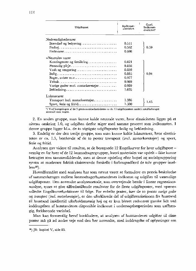
114

10) Jfr. kapitel V, side 85.

J

') Ved beregningen af de 3 gennemsnitselasticiteter er de 13 udgiftsposters andel i totalforbrugetanvendt som vægte.

En anden gruppe, man kunne kalde neutrale varer, hvor elasticiteten ligger på etniveau omkring 1.0, og udgiften derfor stiger med samme procent som indkomsten. Idenne gruppe ligger bl.a. de to vigtigste udgiftsposter bolig og beklædning.

Endelig er der den tredje gruppe, som man kunne kalde luksusvarer, hvor elastici-teten er ca. 1.5, bestående af de to poster transport (incl. motorkøretøjer) og sport,ferie og fritid.

Analysen gav videre til resultat, at de beregnede 12 Engelkurver for hver udgiftspost -nemlig en for hver af de 12 lønmodtagergrupper, hvori materialet var opdelt - ikke kunnebetragtes som sammenfaldende, men at denne opdeling efter bopæl og socialgrupperingsyntes at modsvare faktisk eksisterende forskelle i forbrugsadfærd de tolv grupper imel-lem'0).

Hovedformålet med analysen har som nævnt været at formulere en præcis beskrivelseaf sammenhængen mellem lønmodtagerhusstandenes indkomst og udgifter til væsentligeudgiftsposter. Den anvendte analysemetode, som overvejende består i lineær regressions-analyse, synes at give tilfredsstillende resultater for de fleste udgiftsposter, med »pæne<udledte Engelkurvefunktioner til følge. For enkelte poster, især de to poster varige goderog transport (incl. motorkoretojer), er den uforklarede del af udgiftsvariationen fra husstandtil husstand imidlertid uforholdsmæssig høj og er kun blevet reduceret ganske lidt vedinddragelsen af husstandenes disponible indkomst i undersøgelsesperioden som uafhæn-gig, forklarende variabel.

Man kan formentlig heraf konkludere, at analysen af husstandenes udgifter til disseposter må gå ad andre veje end den her anvendte, med inddragelse of oplysninger om

Udgiftspost Indkomst-elasticitet

NødvendighedsvarerBrændsel og belysning 0.511Fodtøj 0.562Fødevarer 0.608

»Neutrale« varerKontingenter og forsikring 0.821Personlig pleje 0.856Vask og rengøring 0.859Bolig 0.885Bøger, aviser m.v. 0.977Tobak 0.980Varige goder excl. motorkøretøjer 0.989Beklædning 1.035

LuksusvarerTransport incl. motorkøretøjer 1.386Sport, ferie og fritid 1.500

Gnstl.Indkomst-elasticitet'

}

0.59

0.94

115

husstandstype og øvrige milieubetingede faktorer samt ikke mindst af oplysninger ved-rørende indkomstændringer og tidligere perioders forbrugsadfærd. En sådan dynamiskanalyse har imidlertid ligget uden for rammerne af dette arbejde, men det må erkendes,at de her repræsenterede resultater for disse posters vedkommende er utilfredsstillende.

På et par punkter er man gået ud over det ovenfor afgrænsede analyseformål, idet mani et afsluttende kapitel har undersøgt dels, i hvilket omfang de 13 udgiftsposter er korre-lercde, d.v.s. om husstande, der giver meget eller lidt ud til een bestemt udgiftspost udviser,en karaktcrisk udgiftsadfærd med hensyn til een eller flere af dc øvrige poster (har hus-stande med et højt tobaksforbrug et mindre fødevareforbrug end husstande med lavtforbrug af tobak? etc.); dels har man forsøgt at skitsere, hvilken betydning forskelle ihusstandstype (husstandens størrelse og sammensætning) har for husstandenes forbrugs-adfærd i de forskellige indkomstklasser.

Hvad det første problem angår - korrelationen mellem de 13 udgiftsposter - viste deforetagne beregninger, at der kun i ringe grad kunne påvises en sådan korrelation.Kun for så vidt angår de to poster bolig og brændselbelysning fandtes en stærk (positiv)korrelation. Dette resultat falder godt i tråd med hele oplægget til analysen, idet grup-peringen af de mangfoldige varer og tjenester, hvorom oplysninger indhentedes, i etbeskedent antal hovedudgiftsposter netop sigtede mod en gruppering, hvor der kun varen ringe positiv eller negativ korrelation mellem de enkelte grupper. Herved ville mansøge at nå frem til stabile inclkomstudgiftsrelationer, men måtte naturligvis samtidig giveafkald på at beskrive husstandenes forbrugsadfærd overfor enkeltvarer og tjenester.

Med hensyn til husstandstypens betydning for husstandenes forbrugsadfærd viste deforetagne undersøgelser, at selve husstandsstørrelsen var den dominerende faktor, og atman ved den foretagne omregning til beløb pr. person fik elimineret størsteparten afdenne »forstyrrende« påvirkning. For visse udgiftsposter, bl.a. bolig ogfritidsudgjfler, varder imidlertid stadig mærkbare påvirkninger at spore udover persontalseffekten, oggenerelt gjaldt det, som man vel også på forhånd ville vente, at der består economies ofscale, d.v.s., at udgiften pr. person til en given udgiftspost er faldende med persontalletpr. husstand.

Rapportens kapitel I indeholder en oversigt over arbejdets baggrund og tilrettelæggelsesamt over nogle af analysens hovedresultater. Kapitel II er en gennemgang af det an-vendte grundmateriale. Denne gennemgang indeholder dels en beskrivelse af forbrugs-og opsparingsundersøgelsens praktiske udførelse, d.v.s. grundmaterialets indsamling ogbearbejdelse, og dels en udledning af den statistiske usikkerhed, som de fra undersøgelses-materialet udllede tal er behæftet med. I kapitel III afgrænses analyseopgaven, idet for-skellige modeller til beskrivelse af de adspurge husstandes udgiftsadfærd diskuteres, endiskussion der munder ud i en motivering for valget af Engelkurveproblematikken somanalysens hovedemne. Kapitel IV indeholder en detailleret gennemgang af analyse-metoderne. Hvilke funktionstyper skal lægges til grund ved udledningen afEngelkurvcr forde forskellige udgiftsposter? Hvorledes skal de i Engelfunktionen indgående variablenærmere afgrænses? Og ikke mindst, hvorledes skal de anvendte funktionstypers egnethedved beskrivelsen af indkomstudgiftsrelationerne afprøves?

Herefter følger i kapitel V rapportens hovedafsnit, nemlig gennemgangen af analyse-resultaterne, hvorunder især den dobbeltlogaritmiske Engelkurvefunktion, som efter de

116

udførte test for goodness of fit fandtes at være den »bedste« af de 5 afprøvede funktions-typer, kommenteres.

Endelig er der i det afsluttende kapitel VI anført nogle eksempler på nærliggendevideregående beregninger, der skønnes at kunne bidrage til en yderligere præcision i be-skrivelsen af husstandenes forbrugsadfærd, end nærværende analyses hovedredskab,Engelkurven, muliggør. Til »forklaring« af de observerede forskelle i husstandenes ud-gifter til en given udgiftspost fremdrages dels forskelle i husstandenes størrelse og sammen-sætning og dels husstandenes udgifter til een eller flere andre udgiftsposter.

I bilag til rapporten er anført dels en samlet oversigt over analyseresultaterne, derfalder i to afsnit, hovedanalysens resultater, jfr. kap. V og resultater af de videregåendeberegninger jfr. kap. VI, dels det ved analysen benyttede grundmateriale suppleret medvisse yderligere oplysninger, der vil kunne inddrages i eventuelle supplerende analyser.

En liste over den benyttede litteratur er anført side 117-118.

LIST OF LITERATURE

Aitchison, J. and Brown,J. A. C.: The Lognormal Distribution, Cambridge University Press, 1957.

la. Same: "A synthesis of Engel Curve Theory", Review of Economic Studies, vol. XXII, no. 57,1955.

Amundsen, A.: Metoder i Analysen av Forbruksdata, Statistisk Sentralbyrå, Oslo, 1960.

Duesenberry, J.: Income, Saving and the Theory of Consumer Behaviour, Cambridge, 1949.

Durbin and Watson: "Testing for Serial Correlation in Least-Squares Regression", Biometrika37 and 38.

Engel, Ernst: "Die Produktions- und Consumtionsverhaltnisse des Königreichs Sachsen", Zeit-schrift des statistischen Bureau des Koniglich Sachsischen Ministeriums des Innern, 1857.

Forsyth: "The Relationship between Family Size and Family Expenditure", Journal of theRoyal Statistical Society, series A, vol. 123, part 4, 1960.

Friedman, M.: A Theory of the Consumption Function, Princeton, 1957.

Hald, A.: Statistical Theory with Engineering Applications, New York, 1952.

Hendricks, W.: "An Approximation to "Students" Distribution". The Annals of MathematicalStatistics, 1936.

Houthakker, H. S. and Prais, J. S.: The Analysis of Family Budgets With an Application toTwo British Surveys Conducted in 1937-39 and Their Detailed Results. Cambridge UniversityPress, 1955.

I.L.O.: Family Living Studies, A Symposium, Geneva, 1961.

Jørgensen, Erling: "Husholdningsbudgetundersogelser af forbrugsforhold", NationaløkonomiskTidsskrift 1962, 1-2.

Lykke Jensen, E.: Repræsentative undersogelsers teori og metode I. Simpel tilfældig udvælgelse,Copenhagen 1957.

Mc Kay, A. T.: "The Distribution of the Difference between the Extreme Observations and theSample Mean in Samples of n from a Normal Universe". Biometrika, 1935.

Modigliani, F.: Fluctuations in the saving-income Ratio: A Problem in Economic Forecasting.Studies in Income and Wealth, vol. 11, New York, 1949.

Statistical Review, New-Series vol. 2, No. 7.

Statistisk Department (cf. below).

Stone, R.: Measurement of Consumers Expenditure and Behaviour in The United Kingdom1920-38, vol. I, Cambridge, 1954.

Wallander, Jan: Studier i bilismens ekonomi, Uppsala 1958.

Wold, H.: Efterfrågan på jordbruksprodukter och dess kanslighet for pris- och indkomst-forandringer, S.O.U. 1940 : 16, Stockholm, 1940.

«9-

118

Det Statistiske Department:

Statistiske Meddelelser, 4.6.6 Danske Arbejderfamiliers Forbrug, 1. Afdeling, Byarbejdere, Copen-hagen, 1900.

- - 4.11.2 Danske Arbejderfamiliers Forbrug, 2. Afdeling: Landarbejdere,Copenhagen, 1901.

- - 4.40.1 Danske Husholdningsregnskaber, I. Afdeling, Byarbejdere, Copen-hagen, 1912.

- - 4.40.2 Danske Husholdningsregnskaber, 2. Afdeling, Arbejdere og Haand-værkere på Landet, Copenhagen, 1913.

- - 4.40.3 Danske Husholdningsregnskaber, 3. Afdeling, Husmænd og Gaard-mænd, Copenhagen, 1914.

- - 4.54.4 Husholdningsregnskaber for Tjenestemandsfamilier M. Fi., Copen-hagen, 1918.

- - 4.69.5 Husholdningsregnskaber for 1922, Copenhagen, 1925.

- - 4.100.1 Husholdningsregnskaber 1931, Copenhagen, 1936.

- - 4.122.1 Husholdningsregnskaber I Aaret 1/4 1939-29/3 1940 Og i 4 UgersPerioden 11/4-8/5 1942, Copenhagen, 1944.

Statistiske Efterretninger 1915 (no. 24), 1916 (no. 20), 1942 (no. 17), 1949 (no. 58), 1957 (no. 83),and 1958 (no. 46).

Statistiske Undersøgelser, no. 3, Opsparing i Lønmodtagerhusstandene 1955, Copenhagen, 1962.

Statistiske Undersøgelser, no. 6, Lønmodtagerindkomster, Fordeling og Sammensætning, Copenhagen,1962.

Statistical Inquiries, An Analysis of the Personal Income Distribution for Wage and Salary Earners in1955, Copenhagen, 1964.

INDEX

Average expenditure 20, 21 Groups of wage and salary earners 4

Budget relation 103

Calculation of estimates of parameters 45Clothing, expenditure on 8

Coefficient of correlation 52, 57Coefficient of variation 42

constancy of 42average value of 44

Computation programme 52Consumption surveys 3

Correlation between deviations 105

Danish Statistical Department 3

Dansk Sekvens Kalkulator 53Disposable income 35Double-logarithmic function 5Durable goods, expenditure on 9

d-test 49, 71

Elasticity of income 5, 33Engel curves 23Engel functions 23

use of 28variables of 33

Error in the independent variable 27Estimator, efficient 41

Expenditure, average per item 20, 21for different types of household 93 if.

Expenditure concept 14

Expenditure items 4, 7

Frame of the selection 15

F-test 50, 64

Grouping of the observations 38of the expenditures 39

Hendricks, W. 42Houthakker, H. S., and Prais, i. S. 4

Income concept 14

Income elasticity 5

average values of 89Interdependence among households in their

expenditure 25

Layer-effect 25Log-normal distribution 46

transformation of 47

3-parameter case 55

Macro level, Engel curve used on 29Multiple regression analyses 100

Personal hygiene, expenditure on 8

Prais, I. S., and Houthakker, H. S. 4Processing of the material 19

Propensity to consume 33

Regression analysis, versus cross-tabulation 7

modification of 88Regression lines, slopes of 81Response rate 12

Sampling errors 18

Sampling method 15

Saturation expenditure 80Saving concept 14

Social groups 4, 34Statistical Department 3

Survey of income, consumption and saving pat-terns 1955 3

Survey period 15

Systematic errors 18

120

Test, for goodness of fit 48

for identity of regression lines 85

for length of run 49, 71for number of runs 49, 71for parallelism of regression lines 82

Time series versus cross-sectional analysisT-test for

1= 0 78

Types of functions 5

Unit-consumers concept 90

Unit of analysis 13

Variance assumptions 40

x2-test, for constancy of variation 47

26 for normality of deviations 52, 60

Zero-observations 36

APPENDICES

Appendix A. Results of regression analysis.

The results comprise the estimates a, k and b for the five Engel functions

i logy = a + b (logx - gx)

2logy=a+b(3 y=a+b(logxlogx)

Ii i4 y=a±b - -

'X X5 log y = log k + log (a + log x),

x denoting disposable income per person and y denoting expenditure per person on a

given item. Also included are the averages of the dependent variable, log x or and

estimates of the standard errors of a and b, 5a and sj as well as the estimates s and s2denoting the square roots of the variance in the distribution of y within groups and ofthe variance in the distribution of residuals respectively. The tables of result finallycontain the results of the following tests: the correlation coefficient, R, between observedand calculated expenditures, N-test for number of runs and 1-test for number of elementsin the longest run, d-test for size and sign of the residuals, F-test, and x2-test for normalityof the residuals.

The limits of significance (5 or 95 per cent) are given in the following table, separatelyfor each of the twelve groups of wage and salary earners1).

123

1) This table do not include the limits of significance for the N-test the test for number of runs, asthese limits differ from expenditure item to expenditure item within each group of wage and salaryearners, cfr. table V,5.

Limits of significance.

125

Group of wage andsalary earners

Numberof

groupsof 3

house-holds

z -test d-test F-test

l-testdegrees

offreedom

X as

degreesof

freedomd,5

degreesof

freedomF,55

1. Higher sal.public servantsand empl., thecapital 112 7 14.1 110 1.64 111.224 1.31 11

2. Lower publicservants andsal. empi., thecapital 154 9 16.9 512 1.67 153.308 1.26 12

3. Skilled work-ers, the capital 83 7 14.1 81 1.59 82.166 1.36 10

4. Unskilledworkers, thecapital 68 5 11.1 66 1.54 67.136 1.41 10

5. Higher publicservants andsal. empi 70 5 11.1 68 1.55 69.140 1.40 10

6. Lower publicservants andsal. empl 111 7 14.1 109 1.64 110.222 1.31 11

7. Skilled work-ers provincialtowns 51 3 7.8 49 1.46 50.102 1.48 9

8. Unskilledworkers, pro-vincial towns 70 5 11,1 68 1.55 69.140 1.40 10

9. Lower publicservants andsal. empl., ru-raldistr 102 7 14.1 100 1.63 101.204 1.32 11

10. Skilled work-ers, rural di-stricts 51 3 7.8 49 1.46 50.102 1.48 9

11. Unskilledworkers, ruraldistricts 93 7 14.1 91 1.61 92.186 1.34 10

12. Agric. workers,rural distr. . 53 3 7.8 51 1.46 52.106 1.47 9

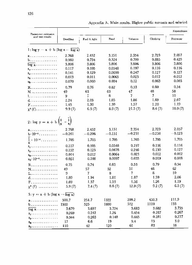
126

Appendix A. Main results. Higher public servants and salaried

Parameter estimatesand test results

Expenditure

Dwelling Fuel & light Food Tobacco Clothing Footwear

1:logy = a + b (1ogx-ij)a 2.768 2.452 3.151 2.354 2.723 2.057b 0.960 0.734 0.524 0.799 0.885 0.429

3.806 3.806 3.806 3.806 3.806 3.806

s1 0.117 0.105 0.0548 0.197 0.116 0.116

s2 0.141 0.120 0.0690 0.247 0.127 0.1270.013 0.011 0.0065 0.023 0.012 0.012

sb 0.070 0.060 0.034 0.12 0.063 0.063

R 0.79 0.76 0.82 0.53 0.80 0.54

N 49 63 63 47 48 58

9 7 8 7 7 10

d 2.24 2.03 1.85 1.86 1.69 2.07F 1.45 1.30 1.59 1.57 1.20 1.192 (f) 9.9 (7) 6.3 (7) 8.9 (7) 21.5 (7) 8.4 (7) 10.0 (7)

2: log y = a + b ( -a 2.768 2.452 3.151 2.354 2.723 2.057b104 -0.261 -0.206 -0.151 -0.231 -0.250 -0.123

1 i0- 1.705 1.705 1.705 1.705 1.705 1.705X

si 0.117 0.105 0.0548 0.197 0.116 0.1160.152 0.123 0.0678 0.246 0.130 0.127

Sa 0.014 0.012 0.0064 0.023 0.012 0.012

Sb 10 0.022 0.108 0.0097 0.035 0.019 0.018

R 0.75 0.74 0.83 0.53 0.79 0.54

N 49 57 52 51 48 62

L 9 7 8 7 8 10

d 1.89 1.94 1.81 1.87 1.59 2.06F. 1.69 1.37 1.53 1.56 1.26 1.19

x2 (f) 5.9 (7) 7.4 (7) 8.8 (7) 12.9 (7) 9.2 (7) 6.5 (7)

3:y = a + b(1ogx-J)a 500.7 251.7 1322 209.2 450.3 111.9

b 1300 525 1880 512 1110 133

log x 3.679 3.697 3.724 3.683 3.682 3.735

s1 0.269 0.242 1.26 0.454 0.267 0.2670.344 0.263 0.148 0.445 0.281 0.277

sa 17 6.6 19 9.4 13 3.0

Sb 110 42 120 61 83 18

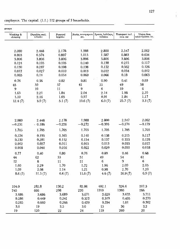
employees. The capital. (1.1.) 112 groups of 3 households.

127

459

5910

5711

61

9

556

4910

586

1.65 2.21 1.84 2.04 2.14 1.98 2.101.10 2.16 1.05 0.97 0.91 2.84 1.17

12.4 (7) 3.9 (7) 5.1 (7) 10.6 (7) 6.0 (7) 25.7 (7) 3.3 (7)

2.080 2.448 2.178 1.988 2.800 2.547 2.062-0.231 -0.186 -0.226 -0.272 -0.393 -0.274 -0.179

1.705 1.705 1.705 1.705 1.705 1.705 1.705

0.124 0.195 0.105 0.140 0.138 0.215 0.1170.130 0.281 0.112 0.154 0.137 0.353 0.1280.012 0.027 0.011 0.015 0.013 0.033 0.0120.018 0.040 0.016 0.022 0.020 0.050 0.018

0.77 0.40 0.80 0.76 0.89 0.46 0.684412

1.601.098.6

104.0245

(7)

628

2.292.08

11.5

282.8666

(7)

5511

1.701.146.6

130.2298

(7)

5111

1.721.21

11.6 (7)

82.06220

4961.960.984.6

402.11910

(7)

5492.092.70

16.9

326.61390

(7)

616

2.051.206.9

107.3186

(7)

groups

Washing &cleaning

Durables excl.vehicles

Personalhygiene

Books, newspapersetc.

Sports, holidays,hobbies

Transport incl.own car

Union fees,subscriptions etc.

2.080 2.448 2.178 1.988 2.800 2.547 2.0620.803 0.574 0.807 1.015 1.387 0.863 0.6343.806 3.806 3.806 3.806 3.806 3.806 3.8060.124 0.195 0.105 0.140 0.138 0.215 0.1170.130 0.287 0.108 0.138 0.132 0.362 0.1260.012 0.027 0.010 0.013 0.012 0.034 0.0120.065 0.14 0.054 0.069 0.066 0.18 0.063

0.76 0.36 0.82 0.81 0.90 0.41 0.69

3.686 3.686 3.689 3.671 3.620 3.635 3.7110.286 0.449 0.241 0.323 0.319 0.495 0.2700.285 0.660 0.266 0.429 0.334 1.01 0.3023.0 19 3.5 3.6 15 36 3.2

19 120 22 24 110 260 20

128

Appendix A. Main results (continued). Higher public servants and

RNidF2 (f)

4: y = a + b (1X

ab10

0.7345II1.951.63

17.2

- X

508.7-290

(7)

0.775710

2.031.18

14.8

253.9-119

(7)

0.845681.941.38

13.1

1328-448

(7)

0.6255

61.750.963.6

209.7-116

(7)

0.7958

7

1.591.1143

456.0-244

(7)

0.586010

2.121.078.6

112.1326

(7)

Sk

RN1

dFz2 (f)

12000

0.7253

92.211.456.05 (9)

1300

0.7661

7

2.051.296.35 (9)

1000

0.846381.931.47

13.70 (9)

2800

0.6249

7

1.871.54

18.97 (9)

6600

0.7950

7

1.741.16

12.26 (9)

110

0.586010

2.091.17

13.15 (9)

I io+ 2.234 2.152 2.021 2.224 2.223 1.977X

si 0.269 0.242 0.126 0.454 0.267 0.2670.388 0.301 0.170 0.472 0.324 0.287

Sa.. 20 7.6 22 10 15 3.1

Sb1O4 28 11 31 14 21 4.5

a -5.687 -5.075 -4.466 -5.258 -5.490 -4.160k 19870 2813 5646 3132 11650 319.8s1 0.117 0.105 0.0548 0.197 0.116 0.116s2 0.141 0.119 0.0664 0.245 0.125 0.125

0.29 0.28 0.16 0.51 0.29 0.36

R 0.70 0.73 0.81 0.62 0.74 0.57N 43 49 50 61 49 581 11 10 8 6 12 10d 1.43 1.61 1.50 1.64 1.22 2.03F. 2.07 1.55 1.81 1.08 1.48 1.15x2 (f) 27.8 (8) 25.0 (7) 8.0 (7) 15.0 (7) 7.6 (7) 5.8 (7)

5: logy = Iogk + 1og (a + logx)

ExpenditureParameter estimates

and test resultsDwelling Fuel & light Food Tobacco Clothing Footwear

salaried employees. The capital. (1.1.) 112 groups of 3 households.

groups

7.6 (7) 42.1 (7) 35.7 (7) 68.4 (7) 35.1 (7) 86.4 (7) 23.1 (7)

129

0.77 0.43 0.79 0.70 0.64 0.34 0.6746 61 55 59 33 51 639 6 11 7 21 9 6

0.774812

1.631.00

10.4

104,4-55.1

(7)

0.4664

82.2621.6

39.6

277.9-154

(7)

0.795112

1.701.21

17.7

131.1-67.0

(7)

0.6653

91.571.77

50.5 (7)

85.26-45.0

0.8551

7

1.501.108.6

398.8-394

(7)

0.464314

2.204.14

80.6

272.0-295

(7)

0.675710

2.051.268.6

109.0-42.8

(7)

1.691.069.13 (9)

2.242.115.93 (9)

1.861.038.73 (9)

2.110.999.41 (9)

0.593.48

19.55 (9)

2.022.79

29.28 (9)

2.121.154.47 (9)

2.207 2.228 2.194 2.281 2.586 2.616 2.067

0.286 0.449 0.241 0.323 0.319 0.495 0.2700.315 0.697 0.305 0.571 0.449 0.956 0.3323.3 20 4.0 4.8 21 31 3.54.6 28 5.6 6.7 29 44 5.0

-5.272 -4.636 -5.278 -5.829 -9.705 -5.440 -4.7891713 1400 2171 4587 2381.108 7003 719.0

0.124 0.195 0.105 0.140 0.138 0.215 0.1170.128 0.283 0.107 1.139 0.257 0.359 0.1250.32 0.55 0.27 0.34 0.051 0.54 0.32

960 990 1000 3500 50.108 7200 320

0.75 0.47 0.75 0.56 0.79 0.54 0.6346 62 37 49 39 45 51

12 8 15 10 11 14 10

1.34 2.22 1.35 1.16 0.81 2.22 1.861.21 2.41 1.60 3.13 1.99 3.73 1.51

Washing & Durables excl. Personal Books, newspapers Sports, holidays, Transport incl. Union fees,cleaning vehicles hygiene etc. bobbies own car subscriptions etc.

130

log y = a + b (

ab10

X

SbiO4RN 69 67 70 72 77 70L 11 7 8 9 9 9dFz2 (f)

Appendix A. Main results (continued). Lower public servants and salaried

ExpenditureParameter estimates

and test resultsDwelling Fuel & light Food Tobacco Clothing Footwear

1: log y = a + b (log x - log x)ablogxSj

RN1

dFx2 (f)

y = a + b (log xablog xs1

s2

sb

768

677

737

709

819

669

1.76 1.97 2.06 1.91 2.12 1.91

1.24 1.31 1.19 1.43 1.14 0.995.2 (9) 25.5 (9) 10.2 (9) 30.4 (9) 8.5 (9) 9.4 (9)

-2.735 2.368 3.152 2.344 2.689 2.063

-0.198 -0.104 -0.118 -0.197 -0.242 -0.132

1.975 1.975 1.975 1.975 1.975 1.975

0.116 0.149 0.0613 0.228 0.129 0.1230.139 0.174 0.0666 0.267 0.145 0.1270.011 0.014 0.0054 0.022 0.012 0.0100.013 0.016 0.0060 0.025 0.014 0.012

0.78 0.46 0.84 0.54 0.82 0.67

2.735 2.368 3.152 2.344 2.689 2.0630.931 0.498 0.533 0.838 1.115 0.6233.745 3.745 3.745 3.745 3.745 3.7450.116 0.149 0.0613 0.228 0.129 0.1230.129 0.171 0.0670 0.273 0.138 0.1220.010 0.014 0.0054 0.022 0.011 0.00980.055 0.073 0.028 0.12 0.059 0.052

0.81 0.49 0.84 0.51 0.84 0.70

1.521.434.8 (9)

1.901.36

16.7

228.0311

(9)

2.031.18

10.9

13121765

(9)

1.981.38

38.8

193.0487

(9)

1.901.263.2

348.61080

(9)

1.761.075.8

107.7161

(9)

- i)453.3

10403.596 3.651 3.652 3.580 3.549 3.6420.268 0.344 0.141 0.525 0.298 0.2820.340 0.362 0.148 0.478 0.333 0.281

13 6.9 16 8.2 11 2.572 37 87 44 58 14

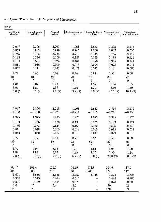
employees. The capital. 1.2 154 groups of 3 households.

131

816

815

955

708

765

807

729

1.84 2.07 2.27 1.91 1.87 1.96 1.851.02 1.89 1.37 1.46 1.20 2.50 1.29

13.8 (9) 8.2 (9) 9.1 (9) 9.9 (9) 3.9 (9) 40.3 (9) 10.2 (9)

2.047 2.396 2.203 1.961 2.653 2.393 2.115-0.188 -0.198 -0.221 -0.211 -0.295 -0.241 -0.150

1.975 1.975 1.975 1.975 1.975 1.975 1.975

0.133 0.236 0.106 0.138 0.155 0.193 0.1240.136 0.323 0.124 0.166 0.180 0.305 0.1380.011 0.026 0.010 0.013 0.015 0.025 0.0110.013 0.030 0.012 0.016 0.017 0.029 0.013

0.77 0.47 0.84 0.74 0.82 0.56 0.688061.771.047.8 (9)

94.10204

8262.081.889.1

204.4686

(9)

8762.231.377.0

119.7333

(9)

7281.911.456.7 (9)

74.49188

6515

1.641.355.0

571.81700

(9)

8261.952.50

34.0

204.9722

(9)

7861.901.248.2

117.0212

(9)

groups

Washing &cleaning

Durables excl.vehicles

Personalhygiene

Books, newspapersetc.

Sports, holidays,hobbies

Transport incl.own car

Union fees,subscriptions etc.

2.047 2.396 2.203 1.961 2.653 2.393 2.1150.853 0.885 0.999 0.946 1.366 1.087 0.6563.745 3.745 3.745 3.745 3.745 3.745 3.7450.133 0.236 0.106 0.138 0.155 0.193 0.1240.134 0.324 0.124 0.167 0.170 0.305 0.1410.011 0.026 0.010 0.013 0.014 0.025 0.0110.057 0.14 0.053 0.071 0.072 0.13 0.060

0.77 0.46 0.84 0.74 0.84 0.56 0.66

3.601 3.536 3.565 3.582 3.745 3.523 3.6230.306 0.543 0.244 0.3 18 - 0.445 0.2860.321 0.759 0.314 0.379 - 1.028 0.3082.6 15 3.4 2.5 - 20 72

14 79 18 13 - 110 9

132

Appendix A. Main results (continued). Lower public servants and salaried

Parameter estimatesand test results

Expenditure

Dwelling Fuel & lightI

Food Tobacco Clothing Footwear

R 0.76 0.57 0.86 0.67 0.84 0.69N 70 65 76 74 73 70

1 18 10 8 9 9 11

d 1.51 1.88 2.11 1.81 1.79 1.86

F 1.61 1.11 1.10 0.83 1.25 1.00

z2 (f) 18.9 (9) 22.0 (9) 10.7 (9) 11.6 (9) 13.2 (9) 13.8 (9)

4:y= a+ b(I_I\x X

a 487.1 230.8 131.9 275.4 576.3 109.9bio_a -167 -54.0 -315 -ill -291 -27.8

1 i0 2.677 2.449 2.452 1.975 1.975 2.471X

0.268 0.344 0.141 - - 0.2820.414 0.389 0.169 - - 0.302

17 7.4 19 - - 2.8

sb'l04 15 7.0 17 - - 2.6

R 0.67 0.53 0.83 0.72 0.68 0.66N 55 61 60 72 61 65

i 21 11 20 9 17 16

d 1.18 1.75 1.68 2.20 1.91 1.61

F 2.39 1.28 1.43 - - 1.15

z2 (f) 33.4 (9) 34.8 (9) 10.1 (9) - - 14.9 (9)

5: log y = log k + log (a + log x)

a -5.496 -4.251 -4.375 -5.257 - -4.639k 13810 772.5 5447 3440 - 631.9

0.116 0.149 0.0613 0.228 - 0.1230.129 0.171 0.0562 0.270 - 0.122

sa 0.25 0.38 0.15 0.49 - 0.296800 310 940 3100 - 240

R 0.78 0.56 0.85 0.65 - 0.69

N 78 67 75 70 - 66

1 8 7 7 9 - 9

d 1.78 1.96 2.13 1.94 - 1.90

F 1.24 1.32 1.13 1.40 - 0.98

z2 (f) 6.66 (11) 20.84 (11) 9.45 (li) 32.74 (li) - 10.14 (11)

employees. The capital. 1.2 154 groups of 3 households.

groups

61 71 57 74 55 58 7415 9 31 8 14 13 8

133

0.76786

0.5880

6

0.838410

0.75748

0.456314

0.476611

0.72729

1.76 2.15 2.16 1.87 1.98 1.95 1.841.10 1.96 1.66 1.42 - 5.34 1.16

25.1 (9) 60.0 (9) 36.9 (9) 19.7 (9) - 229.8 (9) 14.2 (9)

95.79 351.2 122.6 106.6 571.8 374.0 118.7-32.2 -161 -50.4 -46.7 -339 -185 -34.3

2.795 1.975 3.048 1.975 1.975 1.975 2.639

0.306 - 0.244 - - - 0.2860.360 - 0.375 - - - 0.3453.0 - 4.2 - - - 3.52.5 - 3.3 - - - 3.0

0.72 0.62 0.78 0.70 0.69 0.42 0.67

1.39 2.07 1.67 2.35 1.99 1.66 1.561.38 - 2.36 - - - 1.45

29.6 (9) - 54.5 (9) - - - 31.5 (9)

-5.290 -5.376 -5.678 -5.540 -9.633 -5.906 -4.7481849 4920 6099 2558 1564.108 16390 838.4

0.133 0.236 0.106 0.138 0.155 0.193 0.1240.133 0.322 0.122 0.164 0.287 0.303 0.1390.29 0.51 0.22 0.29 0.046 0.40 0.29

970 4700 2900 1500 29.108 15000 340

0.76 0.50 0.83 0.75 0.55 0.43 0.7282 81 94 70 51 82 76

6 5 5 8 23 7 91.86 2.08 2.32 1.95 0.71 1.97 1.901.00 1.86 1.32 1.42 3.42 2.47 1.26

12.40(11) 8.92(11) 8.28(11) 8.48(11) 16.43(11) 39.25(11) 11.95(11)

Washing & Durables excl. Personal Books, newspapers Sports, holidays, Transport incl. Union fees,cleaning vehicles hygiene etc. hobbies own car subscriptions etc.

134

Appendix A. Main results (continued). Skilled workers.

Parameter estimatesand test results

Expenditure

Dwelling Fuel & light Food Tobacco Clothing Footwear

log y = a + b (log x - log x)a 2.616 2.333 3.166 2.450 2.586 1.999b 0.868 0.402 0.685 0.931 1.020 0.502log x 3.705 3.705 3.705 3.705 3.705 3.705s 0.132 0.131 0.0603 0.156 0.116 0.103

0.135 0.116 0.0495 0.176 0.129 0.1010.016 0.014 0.0060 0.021 0.016 0.012

sj 0.084 0.072 0.031 0.11 0.080 0.063

R 0.79 0.57 0.94 0.72 0.84 0.70N 36 33 35 37 40 331 4 4 4 5 5 6d 2.03 1.86 2.11 1.70 2.04 1.94F 1.05 0.78 0.67 1.27 1.23 0.96z2 (f) 4.5 (5) 10.8 (5) 1.4 (5) 6.1 (5) 8.7 (5) 9.8 (5)

2: log y = a + b ( IX

a 2.616 2.333 3.166 2.450 2.586 1.999b104 -0.172 -0.091 -0.138 -0.183 -0.213 -0.106i 10+ 2.171 2.171 2.171 2.171 2.171 2.171X

si 0.132 0.131 0.0603 0.156 0.116 0.103s2 0.142 0.110 0.0563 0.184 0.124 0.0973

0.017 0.013 0.0068 0.022 0.015 0.01251,10 0.018 0.014 0.0072 0.023 0.016 0.012

R 0.76 0.62 0.92 0.69 0.86 0.72N 35 33 31 37 33 341 6 4 6 5 6 6d 1.84 2.07 1.62 1.58 2.23 2.06F 1.16 0.70 0.87 1.38 1.14 0.90z2 (f) 3.3 (5) 4.5 (5) 0.9 (5) 1.1 (5) 6.6 (5) 3.6 (5)

3: y = a + b (log x-i3)a 341.5 207.3 1276 230.9 279.2 94.47b 794 243 2220 593 850 119

log x 3.555 3.624 3.587 3.540 3.521 3.617si 0.304 0.302 0.139 0.360 0.267 0.237sa 0.309 0.249 0.120 0.408 0.278 0.240

14 6.4 20 13 11 2.876 34 110 70 60 15

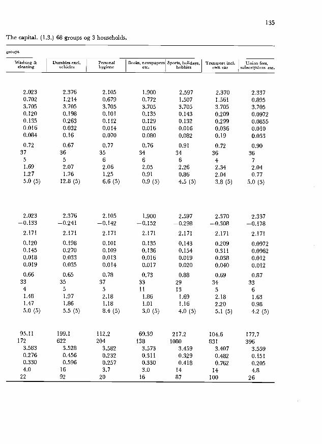
The capital. (1.3.) 68 groups og 3 households.

135

375

365

356

346

346

364

367

1.69 2.07 2.06 2.05 2.26 2.34 2.041.27 1.76 1.25 0.91 0.86 2.04 0.775.0 (5) 12.8 (5) 6.6 (5) 0.9 (5) 4.5 (5) 3.8 (5) 5.0 (5)

2.023 2.376 2.105 1.900 2.597 2.370 2.337-0.133 -0.241 -0.142 -0.152 -0.298 -0.308 -0.178

2.171 2.171 2.171 2.171 2.171 2.171 2.171

0.120 0.198 0.101 0.135 0.143 0.209 0.09720.145 0.270 0.109 0.136 0.154 0.311 0.09620.018 0.033 0.013 0.016 0.019 0.038 0.0120.019 0.035 0.014 0.017 0.020 0.040 0.012

0.66 0.65 0.78 0.73 0.88 0.69 0.873341.481.475.0

95.11172

(5)

3551.971.865.5

199.1622

(5)

3752.181.188.4

112.2204

(5)

3311

1.861.013.0 (5)

69.39138

2913

1.691.164.0

217.21080

(5)

345

2.182.205.1

104.6831

(5)

3361.630.984.2

177.7396

(5)

groups

Washing &cleaning

Durables excl.vehicles

Personalhygiene

Books, newspapersetc.

Sports, holidays,hobbies

Transport inCl.own car

Union fees,subscriptions etc.

2.023 2.376 2.105 1.900 2.597 2.370 2.3370.702 1.214 0.679 0.772 1.507 1.561 0.8953.705 3.705 3.705 3.705 3.705 3.705 3.7050.120 0.198 0.101 0.135 0.143 0.209 0.09720.135 0.263 0.112 0.129 0.132 0.299 0.08550.016 0.032 0.014 0.016 0.016 0.036 0.0100.084 0.16 0.070 0.080 0.082 0.19 0.053

0.72 0.67 0.77 0.76 0.91 0.72 0.90

3.583 3.528 3.582 3.573 3.459 3.407 3.5590.276 0.456 0.232 0.311 0.329 0.482 0.1510.330 0.596 0.257 0.330 0.418 0.762 0.2054.0 16 3.7 3.0 14 14 4.8

22 92 20 16 87 100 26

136

Appendix A. Main results (continued). Skilled workers.

logy = log k + log 1 (a + log x)

RN1

dFz2 (f)

5700

0.783742.011.047.51 (7)

250

0.643341.950.748.49 (7)

3200

0.943462.150.652.46 (7)

6900

0.7237

5

1.71

1.274.95 (7)

13000

0.8440

52.131.164.48 (7)

140

0.6933

62.100.919.49 (7)

Parameter estimatesand test results

Expenditure

Dwelling Fuel & light Food Tobacco Clothing Footwear

R 0.79 0.66 0.93 0.72 0.87 0.70N 37 31 33 37 33 35

1 6 4 6 6 6 8

d 1.88 1.95 1.88 1.62 2.16 2.10F 1.03 0.68 0.75 1.29 1.09 1.03

x2 (f) 2.7 (5) 8.0 (5) 7.1 (5) 6.9 (5) 2.4 (5) 18.9 (5)

4: y = a + b (i iX

a 436.1 204.9 1285 237.4 286.7 93.00biO-4 -126 -44.3 -362 -89.5 -129 -21.8

1 i0X

s1

s2

3.062

0.3040.355

2.660

0.3020.247

2.850

0.1390.165

3.162

0.3600.473

3.281

0.2670.319

2.712

0.2370.242

16 6.3 27 15 13 2.813 5.7 23 12 10 2.5

R 0.76 0.69 0.89 0.67 0.84 0.73

N 27 36 19 31 29 34

1 11 4 13 9 7 8

d 1.53 2.02 1.02 1.32 1.67 2.06F 1.37 0.67 1.42 1.73 1.44 1.04

x2 (f) 6.8 (5) 9.6 (5) 1.7 (5) 12.8 (5) 1.0 (5) 13.3 (5)

a -5.290 -3.934 -4.787 -5.457 -5.697 -4.246k 7424 532.8 10640 7180 16910 343.7

si 0.132 0.131 0.0603 0.156 0.116 0.103

2 0.135 0.113 0.0486 0.176 0.125 0.0311

Sa 0.42 0.52 0.20 0.49 0.35 0.38

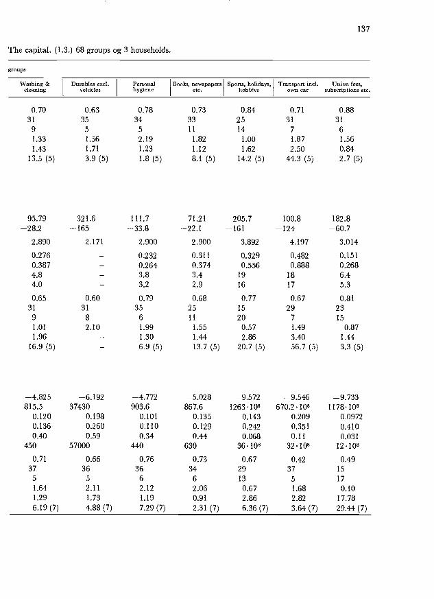
The capital. (1.3.) 68 groups og 3 households.

groups

Washing &cleaning

Durables excl.vehicles

Personalhygiene

Books, newspapersetc.

Sports, holidays,hobbies

Transport incl.own Car

Union fees,subscriptions etc.

137

0.71 0.66 0.76 0.73 0.67 0.42 0.4937 36 36 34 29 37 15

5 5 6 6 13 5 17

1.641.296.19 (7)

2.111.734.88 (7)

2.121.197.29 (7)

2.060.912.31 (7)

0.672.866.36 (7)

1.682.823.64 (7)

0.1017.7829.44 (7)

0.7031

91.331.43

13.5 (5)

95.79-28.2

0.633551.561.713.9 (5)

321.6-165

0.7834

52.191.231.8

111.7-33.8

(5)

0.733311

1.821.128.1 (5)

71.21-22.1

0.8425141.001.62

14.2

205.7-161

(5)

0.7131

7

1.872.50

44.3

100.8124

(5)

0.8831

61.560.842.7

182.8-60.7

(5)

2.890 2.171 2.900 2.900 3.892 4.197 3.014

0.276 - 0.232 0.311 0.329 0.482 0.1510.387 - 0.264 0.374 0.556 0.888 0.2684.8 - 3.8 3.4 19 18 6.44.0 - 3.2 2.9 16 17 5.3

0.65 0.60 0.79 0.68 0.77 0.67 0.81

-4.825 -6.192 -4.772 -5.028 -9.572 -9.546 -9.733815.5 37430 903.6 867.6 1263.108 670.210 117810

0.120 0.198 0.101 0.135 0.143 0.209 0.09720.136 0.260 0.110 0.129 0.242 0.351 0.4100.40 0.59 0.34 0.44 0.068 0.11 0.031

450 57000 440 630 36.108 32.108 12.108

31 31 35 25 15 29 239 8 6 11 20 7 151.01 2.10 1.99 1.55 0.57 1.49 0.871.96 - 1.30 1.44 2.86 3.40 1.44

16.9 (5) - 6.9 (5) 13.7 (5) 20.7 (5) 56.7 (5) 3.3 (5)

138

Appendix A. Main results (continued). Unskilled workers.

Parameter estimatesand test results

Expenditure

Dwelling Fuel & light Food Tobacco Clothing Footwear

log y = a + b (log x - i)a 2.602 2.328 3.157 2.449 2.551 1.968b 0.940 0.312 0.702 1.074 1.047 0.613

3.672 3.672 3.672 3.672 3.672 3.672

si 0.133 0.124 0.0615 0.178 0.152 0.1310.142 0.172 0.0620 0.204 0.156 0.125

s 0.016 0.019 0.0068 0.022 0.017 0.0140.080 0.096 0.035 0.11 0.088 0.070

R 0.80 0.34 0.91 0.72 0.80 0.69N 38 38 40 50 46 431 5 7 5 6 6 7

d 1.83 1.43 1.76 2.06 2.08 2.30F 1.14 1.92 1.02 1.32 1.06 0.92x2 (f) 4.1 (7) 8.0 (7) 8.5 (8) 14.6 (7) 13.3 (7) 7.3 (7)

2: logy = a + b ( i)

a 2.602 2.328 3.157 2.449 2.551 1.968b l0- -0.158 -0.0644 -0.115 -0.170 -0.176 -0.103

2.359 2.359 2.359 2.359 2.359 2.359X

si 0.133 0.124 0.0615 0.178 0.152 0.1310.146 0.167 0.0749 0.221 0.161 0.1280.016 0.018 0.0082 0.024 0.018 0.014

Sbl04 0.014 0.016 0.0072 0.021 0.016 0.012

R 0.78 0.41 0.87 0.66 0.78 0.68N 39 42 33 43 43 421 6 7 11 6 5 6

d 1.75 1.52 1.23 1.77 1.94 2.19F 1.21 1.81 1.48 1.54 1.13 0.96X2 (f) 9.9 (7) 13.7 (7) 7.3 (7) 14.6 (7) 19.7 (7) 7.0 (7)

3: y = a + b (log xa 308.1 211.2 1237 223.7 239.1 85.06b 707 222 2010 551 696000 122

3.473 3.586 3.535 3.467 3.431 3.552

si 0.306 0.286 0.142 0.409 0.350 0.3010.349 0.310 0.157 0.459 0.341 0.271

sa 13 7.4 23 13 11 2.6

Sb 60 36 110 58 48 12

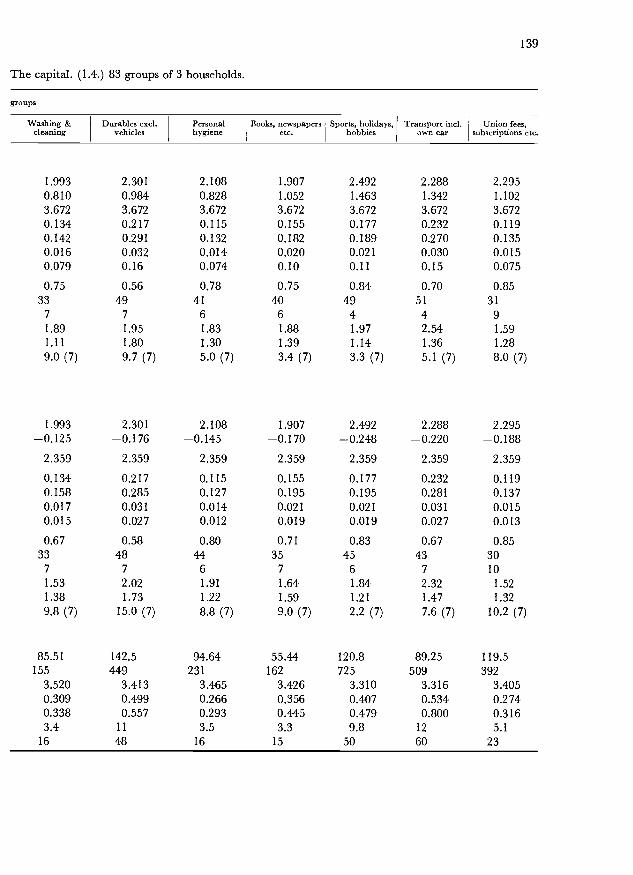
The capital. (1.4.) 83 groups of 3 households.

groups

139

337

497

416

406

494

514

31

9

1.89 1.95 1.83 1.88 1.97 2.54 1.591.11 1.80 1.30 1.39 1.14 1.36 1.289.0 (7) 9.7 (7) 5.0 (7) 3.4 (7) 3.3 (7) 5.1 (7) 8.0 (7)

1.993 2.301 2.108 1.907 2.492 2.288 2.295-0.125 -0.176 -0.145 -0.170 -0.248 -0.220 -0.188

2.359 2.359 2.359 2.359 2.359 2.359 2.359

0.134 0.217 0.115 0.155 0.177 0.232 0.1190.158 0.285 0.127 0.195 0.195 0.281 0.1370.017 0.031 0.014 0.021 0.021 0.031 0.0150.015 0.027 0.012 0.019 0.019 0.027 0.013

0.67 0.58 0.80 0.71 0.83 0.67 0.8533

7

1.531.389.8 (7)

85.51155

487

2.021.73

15.0

142.5449

(7)

4461.911.228.8 (7)

94.64231

357

1.641.599.0 (7)

55.44162

4561.841.212.2 (7)

120.8725

437

2.321.477.6 (7)

89.25509

3010

1.521.32

10.2 (7)

119.5392

1.993 2.301 2.108 1.907 2.492 2.288 2.2950.810 0.984 0.828 1.052 1.463 1.342 1.1023.672 3.672 3.672 3.672 3.672 3.672 3.6720.134 0.217 0.115 0.155 0.177 0.232 0.1190.142 0.291 0.132 0.182 0.189 0.270 0.1350.016 0.032 0.014 0.020 0.021 0.030 0.0150.079 0.16 0.074 0.10 0.11 0.15 0.075

0.75 0.56 0.78 0.75 0.84 0.70 0.85

3.520 3.413 3.465 3.426 3.310 3.316 3.4050.309 0.499 0.266 0.356 0.407 0.534 0.2 740.338 0.557 0.293 0.445 0.479 0.800 0.3 163.4 11 3.5 3.3 9.8 12 5.1

16 48 16 15 50 60 23

Washing & Durables excl. Personal Books, newspapers Sports, holidays, Transport incl. Union fees,cleaning vehicles hygiene etc. hobbies own car subscriptions etc.

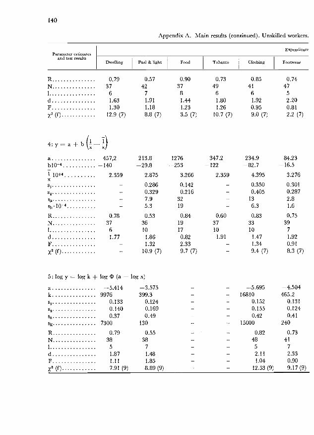
140

Appendix A. Main results (continued). Unskilled workers.

log y = log k + log 1 (a + log x)

Parameter estimatesand test results

Expenditure

Dwelling Fuel & light Food Tobacco Clothing Footwear

R 0.79 0.57 0.90 0.73 0.85 0.74N 37 42 37 49 41 471 6 7 8 6 6 5

d 1.63 1.91 1.44 1.80 1.92 2.20F 1.30 1.18 1.23 1.26 0.95 0.81

x2 (f) 12.9 (7) 8.8 (7) 3.5 (7) 10.7 (7) 9.0 (7) 2.2 (7)

4: y = a + b ( -a 457,2 213.8 1276 347.2 234.9 84.23b104 -140 -29.8 -253 -122 -82.7 -16.5

I 10+ 2.359 2.875 3.266 2.359 4.395 3.276X

St - 0.286 0.142 - 0.350 0.301- 0.329 0.2 16 - 0.405 0.287- 7.9 32 - 13 2.8

b104 - 5.3 19 - 6.3 1.6

R 0.78 0.53 0.84 0.60 0.83 0.75N 37 36 19 37 33 391 6 10 17 10 10 7

d 1.77 1.86 0.82 1.91 1.47 1.92F - 1.32 2.33 - 1.34 0.91

x2 (f) - 10.9 (7) 9.7 (7) - 9.4 (7) 8.3 (7)

RN1

dFz2 (f)

7300

0.7938

51.871.11

7.91 (9)

130

0.5538

7

1.481.858.89

------

(9) -

- 15000

- 0.82- 48- 5- 2.11- 1.04- 12.53 (9)

240

0.7341

7

2.330.909.17 (9)

a -5.414 -3.575 - - -5.695 -4.504k 9976 399.3 - - 16810 465.2

0.133 0.124 - - 0.152 0.131s2 0.140 0.169 - - 0.155 0.124Sa 0.37 0.49 - - 0.42 0.41

The capital. (1.4.) 83 groups of 3 households.

groups

Washing &cleaning

Durables excl.vehicles

Personalhygiene

Books, newspapersetc.

Sports, holidays,hobbies

Transport incl.own car

141

Union fees,subscriptions etc.

0.76 0.68 0.81 0.79 - 0.66 0.6131 49 41 38 - 51 2510 7 6 7 - 4 18

0.7433

7

1.581.19

14.7

87.41-18.6

(7)

0.724862.261.245.4

150.8-52.6

(7)

0.863961.871.21

13.9 (7)

81.23-28.7

0.7837

7

1.361.64

18.2 (7)

55.60-19.0

0.8543

81.461.399.7

121.9-84.3

(7)

0.703312

2.122.24

60.7

85.23-59.8

(7)

0.882811

1.371.33

11.7

230.8-81.0

(7)

1.841.15

11.60 (9)

1.981.75

10.42 (9)

2.061.252.71 (9)

1.851.383.67 (9)

- 2.55- 1.34- 6.06 (9)

0.278.14

23.40 (9)

3.511 4.341 4.420 4.440 5.467 5.483 2.359

0.309 0.499 0.266 0.356 0.407 0.534 -0.402 0.602 0.313 0.564 0.577 0.918 -4.1 12 3.4 4.2 12 14 -2.3 6.0 1.7 2.1 6.8 7.7 -0.67 0.71 0.88 0.70 0.81 0.66 0.86

29 42 35 37 31 29 2615 9 9 7 11 14 11

-5.057 -5.537 -5.118 -5.703 - -6.443 -9.6181204 6530 1758 3877 - 70590 836.8.108

0.134 0.217 0.115 0.155 - 0.232 0.1190.144 0.287 0.128 0.182 - 0.269 0.3390.39 0.60 0.33 0.42 - 0.61 0.039

800 8200 1000 3600 - 120000 130.108

1.18 2.02 1.62 0.98 1.05 1.84 1.861.69 1.45 1.39 2.51 2.01 2.96 -

16.7 (7) 9.8 (7) 8.6 (7) 32.6 (7) 16.8 (7) 77.4 (7) -

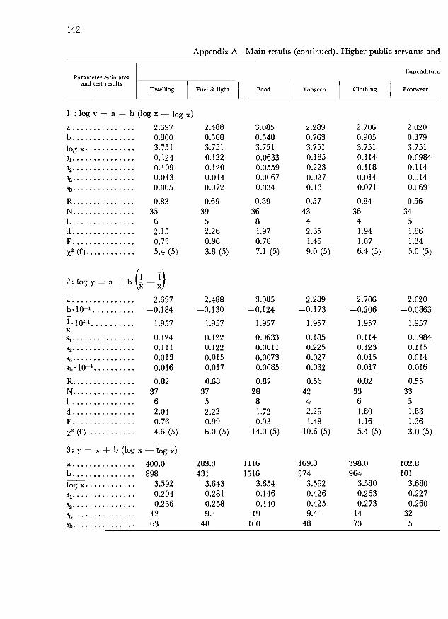
142

Appendix A. Main results (continued). Higher public servants and

ExpenditureParameter estimates

and test resultsDwelling Fuel & light Food Tobacco Clothing Footwear

1: log y = a + b (log x - log x)ab

s1

Sa

Sb

RN 351 6

d 2.15F 0.73

x2 (f) 5.4 (5)

log y = a + b - f)

a 2.697b10-4 -0.1841. 10-l-4 1.957Xs1 0.124

0.1110.013

Sj 10 0.016

R 0.82N 37 37 28 42 33 331 6 5 8 4 6 5

d 2.04 2.22 1.72 2.29 1.80 1.83F. 0.76 0.99 0.93 1.48 1.16 1.36

x2 (f) 4.6 (5) 6.0 (5) 14.0 (5) 10.6 (5) 5.4 (5) 3.0 (5)

y = a + b (log x -Ï)a 400.0 283.3 1116 169.8 398.0 102.8b 898 431 1516 374 964 101

log x 3.592 3.643 3.654 3.592 3.580 3.680Sl 0.294 0.281 0.146 0.426 0.263 0.227

2 0.236 0.258 0.140 0.425 0.273 0.260Sa 12 9.1 19 9.4 14 32

Sb 63 48 100 48 73 5

2.697 2.488 3.085 2.289 2.706 2.0200.800 0.568 0.548 0.763 0.905 0.3793.751 3.751 3.751 3.751 3.751 3.7510.124 0.122 0.0633 0.185 0.114 0.09840.109 0.120 0.0559 0.223 0.118 0.1140.013 0.014 0.0067 0.027 0.014 0.0140.065 0.072 0.034 0.13 0.071 0.069

0.83 0.69 0.89 0.57 0.84 0.5639

5

368

434

364

345

2.26 1.97 2.35 1.94 1.860.96 0.78 1.45 1.07 1.343.8 (5) 7.1 (5) 9.0 (5) 6.4 (5) 5.0 (5)

2.488 3.085 2.289 2.706 2.020-0.130 -0.124 -0.173 -0.206 -0.0863

1.957 1.957 1.957 1.957 1.957

0.122 0.0633 0.185 0.114 0.09840.122 0.0611 0.225 0.123 0.1150.015 0.0073 0.027 0.015 0.0140.017 0.0085 0.032 0.017 0.016

0.68 0.87 0.56 0.82 0.55

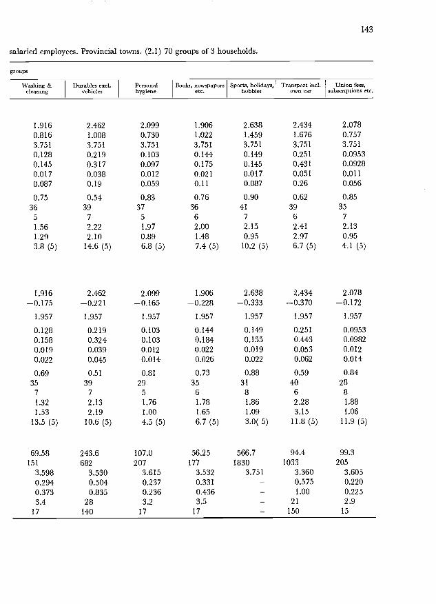
salaried employees. Provincial towns. (2.1) 70 groups of 3 households.

143

365

397

375

366

41

7

396

357

1.56 2.22 1.97 2.00 2.15 2.41 2.131.29 2.10 0.89 1.48 0.95 2.97 0.953.8 (5) 14.6 (5) 6.8 (5) 7.4 (5) 10.2 (5) 6.7 (5) 4.1 (5)

1.916 2.462 2.099 1.906 2.638 2.434 2.078-0.175 -0.221 -0.165 -0.228 -0.333 -0.370 -0.172

1.957 1.957 1.957 1.957 1.957 1.957 1.957

0.128 0.219 0.103 0.144 0.149 0.251 0.09530.158 0.324 0.103 0.184 0.155 0.443 0.09820.019 0.039 0.012 0.022 0.019 0.053 0.0120.022 0.045 0.014 0.026 0.022 0.062 0.014

0.69 0.51 0.81 0.73 0.88 0.59 0.8435

7

1.321.53

13.5 (5)

69.58151

397

2.132.19

10.6

243.6682

(5)

2951.761.004.5

107.0207

(5)

3561.781.656.7 (5)

56.25177

31

81.861.093.0( 5)

566.71830

4062.283.15

11.8

94.41033

(5)

2881.881.06

11.9

99.3205

(5)

groups

Washing &cleaning

Durables excl.vehicles

Personalhygiene

Books, newspapersetc.

Sports, holidays,hobbies

Transport incl.Own car

Union fees,subscriptions etc.

1.916 2.462 2.099 1.906 2.638 2.434 2.0780.816 1.008 0.730 1.022 1.459 1.676 0.7573.751 3.751 3.751 3.751 3.751 3.751 3.7510.128 0.219 0.103 0.144 0.149 0.251 0.09530.145 0.317 0.097 0.175 0.145 0.431 0.09280.017 0.038 0.012 0.021 0.017 0.051 0.0110.087 0.19 0.059 0.11 0.087 0.26 0.056

0.75 0.54 0.83 0.76 0.90 0.62 0.85

3.598 3.530 3.615 3.532 3.751 3.360 3.6050.294 0.504 0.237 0.331 - 0.575 0.2200.373 0.835 0.236 0.436 - 1.00 0.2253.4 28 3.2 3.5 - 21 2.9

17 140 17 17 - 150 15

144

Appendix A. Main results (continued). Higher public servants and

Parameter estimatesand test results

Expenditure

Dwelling Fuel & light Food Tobacco Clothing Footwear

R 0.87 0.74 0.88 0.69 0.85 0.58N 39 35 32 38 33 321 6 5 8 5 6 5

d 2.12 2.22 1.90 2.32 1.78 1.83F 0.64 0.84 0.92 1.00 1.07 1.32

x2 (f) 12.6 (5) 3.6 (5) 12.5 (5) 6.5 (5) 7.l( 5) 3.1 (5)

4:y= a+ b()a 393.3 290.2 1144 169.7 396.2 102.4biO-4 -140 -71.9 -256 -56.0 -143 -19.5llo+. .. 2.972 2.483 2.400 2.987 3.074 2.336X

s1 0.294 0.281 0.146 0.426 0.263 0.2272 0.286 0.298 0.190 0.496 0.340 0.269

sa 15 11 26 11 18 3.4Sb l0- 11 9.3 24 7.9 13 3.2

R 0.85 0.69 0.79 0.63 0.80 0.60N 27 33 20 30 25 351 12 8 26 10 13 5

d 1.50 1.90 1.27 1.89 1.13 1.74F 0.95 1.12 1.71 1.36 1.67 1.41

x2 (f) 4.8 (5) 1.2 (5) 33.4 (5) 11.9 (5) 9.9 (5) 10.7 (5)

5: logy = log k + log (a + log x)

a -5.163 -4.500 -4.439 -5.063 - -3.884k 6390 1375 5023 2081 - 237.2

0.124 0.122 0.0633 0.185 - 0.094s2 0.107 0.119 0.0551 0.221 - 0.114S5 0.40 0.42 0.22 0.58 - 0.39Sk 4400 710 1300 2000 - 77

R 0.83 0.73 0.88 0.68 - 0.58N 34 37 34 43 - 341 6 5 8 4 - 5

d 2.22 2.28 2.09 2.35 - 1.86F 0.75 0.95 0.76 1.43 - 1.33x2 (f) 2.53 (7) 4.12 (7) 9.05 (7) 8.82 (7) - 2.01 (7)

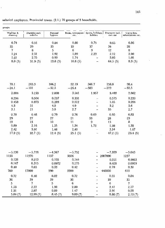
salaried employees. Provincial towns. (2.1.) 70 groups of 3 households.

groups

145

-5.198 -5.718 -4.967 -5.752 - -7.399 -5.043

780 17000 590 3300 - 440000 610

0.72 0.48 0.82 0.72 - 0.55 0.84

1.531.31

5.84 (7)

2.222.07

12.99 (7)

1.980.898.45 (7)

2.001.479.89 (7)

- 2.41- 2.91- 8.86 (7)

2.170.932.13 (7)

0.7435

7

1.241.61

8.0 (5)

70.1-24.1

0.5129

82.312.75

31.9

263.9-101

(5)

0.8435

5

1.920.99

13.8

106.2-32.5

(5)

0.8035

61.891.74

16.8 (5)

52.19-26.4

0.7537

92.29

--

566.7-383

0.653412

2.123.03

64.5

158.0-219

(5)

0.8628

82.001.058.3

98.4-32.5

(5)

2.884 3.233 2.808 3.541 1.957 3.493 2.862

0.294 0.504 0.237 0.331 - 0.575 0.2200.458 0.873 0.289 0.512 - 1.05 0.2844.3 31 4.0 4.0 - 3.2 3.63.1 21 3.0 2.7 - 35 2.7

0.70 0.48 0.79 0.76 0.69 0.60 0.8329 27 27 21 33 28 2913 13 10 11 9 13 8

36 39 39 36 - 39 355 7 5 6 - 6 7

1133 11970 1137 3606 - 2087000 12370.128 0.219 0.103 0.144 - 0.251 0.09530.147 0.315 0.0972 0.175 - 0.428 0.09190.40 0.65 0.33 0.42 - 0.70 0.30

0.89 2.16 1.35 1.34 1.73 1.98 1.382.42 3.01 1.48 2.40 - 3.34 1.67

17.9 (5) 32.7 (5) 12.4 (5) 25.1 (5) - 47.2 (5) 23.4 (5)

Washing & Durables excl. Personal Books, newspapers Sports, holidays, Transport incl. Union fees,cleaning vehicles hygiene etc. hobbies Own car subscriptions etc.

146

Appendix A. Main results (continued). Lower public servants and

Parameter estimatesand test results

Expenditure

Dwelling Fuel & light Food Tobacco Clothing Footwear

log y = a + b (log x - j)a 2.619 2.405 3.071 2.259 2.628 2.002b 0.856 0.440 0.640 0.896 1.017 0.567

log x 3.656 3.656 3.656 3.656 3.656 3.6560.131 0.157 0.0660 0.203 0.121 0.1200.137 0.157 0.0723 0.253 0.127 0.1260.013 0.015 0.0069 0.024 0.012 0.0120.061 0.070 0.032 0.11 0.057 0.056

R 0.80 0.51 0.88 0.60 0.86 0.69N 48 63 48 54- 60 571 7 9 6 6 6 6d 1.77 2.20 1.90 2.14 2.08 2.05F 1.09 1.00 1.20 1.56 1.10 1.10

x2 (f) 9.4 (7) 15.0 (7) 5.8 (7) 32.0 (7) 6.1 (7) 10.9 (7)

2: logy = a + b

a(

2.619 2.405 3.071 2.259 2.628 2.002bl04 -0.146 -0.0720 -0.108 -0.151 -0.173 -0.9671. l0 2.484 2.484 2.484 2.484 2.484 2.484X

s 0.131 0.157 0.0660 0.203 0.121 0.120

sa 0.140 0.160 0.0781 0.257 0.134 0.1280.013 0.015 0.0074 0.024 0.013 0.012

b104 0.011 0.012 0.0060 0.020 0.010 0.0099

R 0.79 0.49 0.86 0.59 0.85 0.68N 48 61 53 55 55 581 7 9 9 6 6 6d 1.69 2.13 1.65 2.09 1.88 1.99

F 1.15 1.04 1.40 1.60 1.23 1.13

x2 (f) 3.9 (7) 9.6 (7) 4.3 (7) 18.9 (7) 7.7 (7) 15.5 (7)

3:y = a + b(logx-logx)a 311.3 245.3 1021 149.0 294.7 91.32b 755 292 1610 365 813 134

3.448 3.550 3.517 3.447 3.424 3.5270.302 0.362 0.152 0.466 0.280 0.277

s2 0.312 0.313 0.167 0.490 0.338 0.290sa 10 7.5 17 7.9 11 2.6

48 35 80 36 50 12

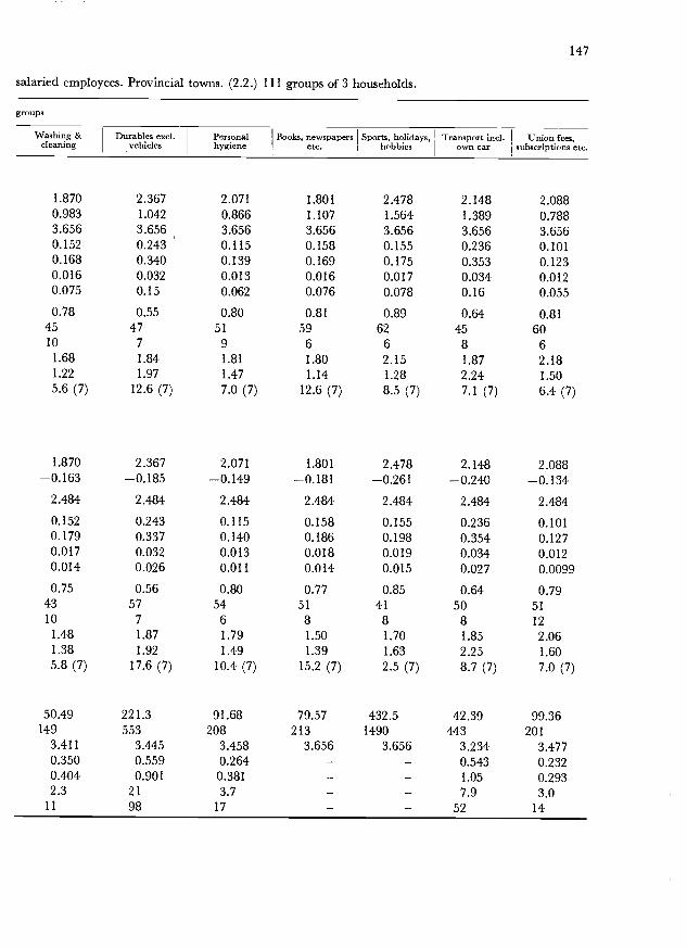
salaried employees. Provincial towns. (2.2.) 111 groups of 3 households.

147

4510

477

51

959

662

645

860

61.68 1.84 1.81 1.80 2.15 1.87 2.181.22 1.97 1.47 1.14 1.28 2.24 1.505.6 (7) 12.6 (7) 7.0 (7) 12.6 (7) 8.5 (7) 7.1 (7) 6.4 (7)

1.870 2.367 2.071 1.801 2.478 2.148 2.088-0.163 -0.185 -0.149 -0.181 -0.261 -0.240 -0.134

2.484 2.484 2.484 2.484 2.484 2.484 2.484

0.152 0.243 0.115 0.158 0.155 0.236 0.1010.179 0.337 0.140 0.186 0.198 0.354 0.1270.017 0.032 0.013 0.018 0.019 0.034 0.0120.014 0.026 0.011 0.014 0.015 0.027 0.0099

0.75 0.56 0.80 0.77 0.85 0.64 0.794310

1.481.385.8 (7)

50.49149

577

1.871.92

17.6

221.3553

(7)

5461.791.49

10.4

91.68208

(7)

51

81.501.39

15.2

79.57213

(7)

41

81.701.632.5

432.51490

(7)

5081.852.258.7 (7)

42.39443

51

12

2.061.607.0 (7)

99.36201

groups

Washing &cleaning

Durables excl.vehicles

Personalhygiene

Books, newspapersetc.

Sports, holidays, Transport incl.hobbies own car

Union fees,subscriptions etc.

1.870 2.367 2.071 1.801 2.478 2.148 2.0880.983 1.042 0.866 1.107 1.564 1.389 0.7883.656 3.656 3.656 3.656 3.656 3.656 3.6560.152 0.243 0.115 0.158 0.155 0.236 0.1010.168 0.340 0.139 0.169 0.175 0.353 0.1230.016 0.032 0.013 0.016 0.017 0.034 0.0120.075 0.15 0.062 0.076 0.078 0.16 0.055

0.78 0.55 0.80 0.81 0.89 0.64 0.81

3.411 3.445 3.458 3.656 3.656 3.234 3.4770.350 0.559 0.264 - - 0.543 0.2320.404 0.901 0.381 - - 1.05 0.2932.3 21 3.7 - - 7.9 3.0

11 98 17 - - 52 14

148

log y = log k + log cD (a + log x)

Appendix A. Main results (continued). Lower public servants and

Parameter estimatesand test results

Expenditure

Dwelling Fuel & light Food Tobacco Clothing Footwear

R 0.84 0.62 0.89 0.70 0.84 0.72

N 52 63 53 61 51 60

1 7 8 9 7 7 6

d 1.66 2.12 1.83 1.98 1.77 2.00

F 1.07 0.75 1.21 1.10 1.46 1.09

x2 (f) 13.5 (7) 3.8 (7) 4.0 (7) 6.0 (7) 11.9 (7) 21.5 (7)

(1 i4: y = a + bX

a 298.9 248.6 1039 155.9 287.1 91.01

b104 -89.4 -37.2 -197 -43.1 -93.8 -17.5

10 4.3 16 3.198 3.474 4.055 4.523 3.450X

s1 0.302 0.362 0.152 0.466 0.280 0.277

s2 0.372 0.355 0.219 0.555 0.417 0.317

sa 12 8.6 23 9.4 14 2.9

sb 10-t 6.1 5.2 13 4.7 6.7 1.6

R 0.81 0.56 0.83 0.67 0.80 0.72

N 39 63 35 49 43 55

1 11 11 21 11 18 5

d 1.18 1.83 1.18 1.57 1.16 1.76

F 1.52 0.96 2.08 1.41 2.22 1.31

x2 (f) 14.7 (7) 12.4 (7) 9.0 (7) 12.2 (7) 19.5 (7) 27.3 (7)

RN1

dFZ2 (f)

3800

0.8148

7

1.831.076.57 (9)

280

0.6265

92.211.00

15.03 (9)

1500

0.8953

7

1.971.16

10.73 (9)

3300

0.685462.151.54

25.49 (9)

10000

0.8460

6

2.131.088.41 (9)

160

0.7158

6

2.101.09

14.15 (9)

a -5.200 -3.971 -4.595 -5.307 -5.625 -4.379k 6918 685.4 6896 3753 17720 435.3

0.131 0.157 0.0660 0.203 0.121 0.1200.136 0.157 0.0711 0.252 0.126 0.1250.30 0.44 0.16 0.46 0.27 0.31

groups

Washing &cleaning

Durables excl.vehicles

Personalhygiene

salaried employees. Provincial towns. (2.2.) 111 groups of 3 households.

Books, newspapersetc.

Sports, holidays,hobbies

Transport incl.Own car

Union fees,subscriptions etc.

0.88 1.69 1.41 2.02 1.78 1.80 1.601.98 2.83 2.69 - - - 2.35

37.7 (7) 98.4 (7) 42.7 (7) - - - 18.4 (7)

149

1800 14000 1000 3700 2000.108 - 560

1.671.219.69 (9)

1.961.94

13.51 (9)

1.871.417.16 (9)

1.801.14

11.85 (9)

0.962.898.00 (9)

- 2.24- 1.45- 10.51 (9)

0.824910

1.311.33

14.3 (7)

48.56-17.1

0.473513

1.772.60

91.1

199.0-66.8

(7)

0.765210

1.782.09

B6.9

91.60-24.5

(7)

0.4245

9

2.07--

79.57-31.7

0.743713

2.02--

432.5-218

0.6440

9

1.863.72

100.5

246.0-107

(7)

0.815312

2.091.608.5

105.5-23.7

(7)

4.683 4.541 4.110 2.484 2.484 2.484 3.689

0.350 0.559 0.264 - - - 0.2320.492 0.941 0.432 - - - 0.3552.8 22 4.3 - - - 3.81.4 10 2.1 - - - 2.1

0.76 0.52 0.73 0.41 0.65 0.58 0.7435 36 39 31 33 36 4717 13 18 17 15 9 16

0.79 0.46 0.76 0.79 0.65 - 0.8246 47 49 55 45 - 6210 7 5 6 12 - 5

-5.535 -5.694 -5.230 -5.855 -9.450 - -5.0162508 11440 2077 4643 677.4.108 - 1437

0.152 0.243 0.115 0.158 0.155 - 0.1010.167 0.339 0.136 0.159 0.263 - 0.1220.34 0.53 0.26 0.34 0.69 - 0.23

150

Appendix A. Main results (continued). Skilled workers.

Parameter estimatesand test results

Expenditure

Dwelling Fuel & light Food Tobacco Clothing Footwear

log y = a + b (log x Ïj)a 2.504 2.368 3.045 2.313 2.467 1.872

b 0.750 0.276 0.601 1.068 1.103 0.670

log x 3.575 3.575 3.575 3.575 3.575 3.575

si 0.112 0.123 0.0521 0.181 0.123 0.108

s2 0.102 0.135 0.0673 0.187 0.137 0.09650.014 0.019 0.0094 0.026 0.019 0.0140.077 0.10 0.051 0.14 0.10 0.073

R 0.81 0.36 0.86 0.73 0.83 0.79

N 24 25 28 18 30 29

1 6 5 5 6 4 6

d 2.34 1.42 2.46 1.57 2.44 2.10

F 0.83 1.21 1.67 1.07 1.25 0.79

x2 (f) 7.0 (3) 6.5 (3) 3.9 (3) 5.8 (3) 2.1 (3) 2.8 (3)

2: log y = a + b ( -a 2.504 2.368 3.045 2.313 2.467 1.872

b104 -0.117 -0.0550 -0.0933 - 0.164 -0.173 -0.105

2.901 2.901 2.901 2.901 2.901 2.901X

s1 0.112 0.123 0.0521 0.181 0.123 0.1080.106 0.129 0.0711 0.194 0.139 0.09780.015 0.018 0.0099 0.027 0.020 0.014

5b l0 0.013 0.016 0.0085 0.023 0.017 0.012

R 0.80 0.45 0.84 0.71 0.83 0.79

N 28 26 28 19 28 28

4 5 7 6 5 6

d 2.14 1.54 2.18 1.50 2.36 2.05

F 0.89 1.10 1.86 1.15 1.29 0.82

x2 (f) 5.3 (3) 9.6 (3) 0.9 (3) 6.4 (3) 3.2 (3) 5.4 (3)

3: y = a + b (log x - log x)a 282.9 232.1 1016 161.0 222.8 67.45b 545 236 1560 515 693 116

log x 3.465 3.512 3.483 3.411 3.414 3.474s1 0.259 0.252 0.120 0.417 0.282 0.249

0.242 0.264 0.162 0.442 0.314 0.21810 8.7 24 11 11 2.1

60 50 140 70 68 13

Provincial towns. (2.3.) 51 groups of 3 households.

151

21

7

235

216

295

288

236

325

1.74 2.20 1.69 2.14 1.90 1.86 2.641.52 2.88 0.68 1.04 0.87 1.92 0.660.7 (3) 2.2 (3) 3.7 (3) 4.3 (3) 5.0 (3) 0.5 (3) 13.0 (3)

1.846 2.230 1.963 1.703 2.345 2.055 2.285-0.135 -0.244 -0.123 -0.136 -0.266 -0.243 -0.124

2.901 2.901 2.901 2.901 2.901 2.901 2.901

0.121 0.203 0.110 0.135 0.151 0.244 0.09770.159 0.338 0.087 0.138 0.140 0.345 0.08490.022 0.047 0.012 0.019 0.020 0.048 0.0120.019 0.041 0.010 0.017 0.017 0.041 0.010

0.71 0.65 0.86 0.76 0.92 0.64 0.8725

726

419

6

254

266

236

296

1.55 2.27 1.80 2.13 1.90 1.82 2.351.71 2.78 0.63 1.03 0.85 1.99 0.751.2 (3) 0.1 (3) 2.7 (3) 4.1 (3) 0.4 (3) 1.2 (3) 7.8 (3)

59.67 61.87 78.30 41.84 67.65 72.2 163.8147 695 169 107 731 414 353

groups

Washing &cleaning

Durables excl.vehicles

Personalhygiene

Books, newspapersetc.

Sports, holidays,hobbies

Transport incl.own car

Union fees,subscriptions etc.

1.846 2.230 1.963 1.703 2.345 2.055 2.2850.898 1.501 0.767 0.858 1.679 1.576 0.7993.575 3.575 3.575 3.575 3.575 3.575 3.5750.121 0.203 0.110 0.135 0.151 0.244 0.09770.149 0.344 0.0905 0.138 0.141 0.338 0.07940.021 0.048 0.013 0.019 0.020 0.047 0.0110.11 0.26 0.069 0.10 0.11 0.26 0.60

0.75 0.64 0.85 0.76 0.91 0.66 0.88

3.441 3.287 3.454 3.436 3.290 3.332 3.4540.279 0.466 0.252 0.312 0.348 0.563 0.2250.367 0.748 0.205 0.354 0.380 0.813 0.1763.3 11 2.4 2.2 5.8 10 4.3

20 92 14 14 50 74 26

152

Appendix A. Main results (continued). Skilled workers.

logy = log k + log I (a + log x)

RN1

dFx2 (f)

2300

0.8026

42.450.803.56 (5)

180

0.5325

5

1.471.142.39 (5)

1600

0.8528

52.481.610.61 (5)

19000

0.701861.571.055.64 (5)

24000

0.823042.491.201.55 (5)

330

0.792962.170.775.57 (5)

Parameter estimatesand test results

Expenditure

Dwelling Fuel & light Food Tobacco Clothing Footwear

R 0.79 0.56 0.85 0.73 0.82 0.80N 26 24 28 23 28 31

1 7 5 7 6 5 6d 2.16 1.53 2.29 1.39 2.18 2.12F 0.87 0.87 1.81 1.12 1.24 0.76x2 (f) 2.5 (3) 6.9 (3) 1.4 (3) 6.9 (3) 2.6 (3) 2.7 (3)

4: y = a + b ( -a 290.4 229.8 1026 159.2 232.7 67.47bb-4 -67.8 -34.7 -202 -61.1 -83.1 -15.2I l0+ 3.650 3.373 3.535 4.265 4.085 3.645X

s 0.259 0.252 0.120 0.417 0.282 0.249

2 0.283 0.261 0.191 0.515 0.371 0.23612 8.6 28 13 14 2.3

sjybO4 8.9 6.6 26 9.1 9.5 1.7

R 0.73 0.60 0.80 0.69 0.78 0.78N 24 24 21 23 21 291 7 6 16 6 7 6d 1.66 1.64 1.71 1.18 1.63 1.88F 1.20 0.85 2.53 1.53 1.73 0.90x2 (f) 8.2 (3) 10.3 (3) 3.1 (3) 5.5 (3) 1.1 (3) 1.3 (3)

a -4.855 -3.399 -4.428 -5.701 -5.797 -4.629k 3229 414.1 5711 12470 22650 517.4s1 0.112 0.123 0.0521 0.181 0.123 0.108

2 0.100 0.131 0.0661 0.185 0.135 0.09480.45 0.69 0.22 0.67 0.45 0.44

Provincial towns. (2.3.) 51 groups of 3 households.

153

1400 - 730 870 3400000 - 1600

groups

Washing &cleaning

Durables excl.vehicles

Personalhygiene

Books, newspapersetc.

Sports, holidays,hobbies

Transport incl.own car

Union fees,subscriptions etc.

0.73 0.74 0.86 0.75 0.91 0.62 0.8923 25 21 26 21 17 31

7 6 6 4 8 10 5

1.64 2.14 1.83 2.11 1.12 1.34 2.481.73 2.57 0.66 1.29 1.19 2.09 0.611.3 (3) 9.3 (3) 4.8 (3) 11.0 (3) 2.8 (3) 7.8 (3) 5.4 (3)

61.01 41.89 77.42 41.42 57.15 193.4 164.0-18.3 -79.4 -21.6 -13.2 -83.0 -113 -44.3

3.888 5.608 3.847 4.014 5.491 2.901 3.827

0.279 0.466 0.252 0.312 0.348 - 0.2250.414 0.836 0.224 0.394 0.550 - 0.2263.9 9.8 2.6 2.5 7.9 - 5.52.8 11 1.9 1.8 7.7 - 4.0

0.69 0.73 0.85 0.73 0.84 0.24 0.84

1.721.520.56 (5)

- 1.82- 0.63- 3.48 (5)

2.191.027.86 (5)

2.290.823.77 (5)

- 2.65- 0.64- 7.93 (5)

19 23 17 23 19 17 277 7 7 5 8 10 61.31 2.02 1.58 1.83 0.53 2.24 1.672.20 3.21 0.79 1.59 2.50 - 1.015.5 (3) 11.8 (3) 8.1 (3) 9.2 (3) 13.6 (3) - 10.3 (3)

0.71 - 0.84 0.74 0.89 - 0.8921 - 23 29 28 - 34

7 - 6 5 8 - 5

-5.255 - -4.906 -5.154 -7.231 - -4.9911531 - 1016 895.9 1758000 - 2492

0.121 - 0.110 0.135 0.151 - 0.09770.149 - 0.0873 0.136 0.137 - 0.07820.46 - 0.43 0.52 0.54 - 0.38

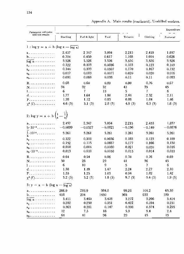
154

Parameter estimatesand test results

Appendix A. Main results (continued). Unskilled workers.

Expenditure

x)

2 347 3.034 2.215 2.453 1.8570.430 0.617 1.168 1.014 0.6263.526 3.526 3.526 3.526 3.526

2 (f) 4.6 (5)

2: logy = a + b (-)a 2.457b l0 -0.0899

1. l0+ 3.261X

s1 0.122s2 0.152

0.0180.013

R 0.64N 30 281 6 10

dFy2 (f)

3: y = a + b (log x - log x)a 266.0 219.9b 418 204log x 3.411

si 0.2820.363

12

sb 64

327

3213

435

357

456

1.64 1.80 2.44 2.32 2.111.12 0.83 0.86 1.84 1.463.1 (5) 2.8 (5) 4.9 (5) 6.3 (5) 1.6 (5)

2.347 3.034 2.215 2.453 1.857-0.0527 -0.0821 -0.156 -0.140 -0.0876

3.261 3.261 3.261 3.261 3.261

0.103 0.0656 0.183 0.123 0.1090.115 0.0667 0.177 0.166 0.1300.014 0.0080 0.021 0.020 0.0160.010 0.0058 0.015 0.014 0.011

0.54 0.86 0.78 0.76 0.69

0.183 0.123 0.1090.109 0.0597 0.170 0.167 0.1320.013 0.0071 0.020 0.020 0.0160.069 0.038 0.11 0.11 0.083

0.60 0.89 0.80 0.76 0.67

1.58 1.491.55 1.253.2 (5) 3.2 (5)

299

1.471.031.8

984.01450

(5)

415

2.240.949.7 (5)

99.26365

367

2.271.829.4

164.2633

(5)

456

2.101.421.9 (5)

65.59109

Dwelling

log y = a + b (log x log

a 2.457b 0.704log x 3.526si 0.122

0.1440.017

sb 0.091

R 0.68N 341 6d 1.77F 1.38

3.460 3.428 3.272 3.266 3.4140.238 0.151 0.422 0.284 0.2510.281 0.147 0.398 0.374 0.2957.5 18 5.9 9.4 2.4

41 96 29 45 13

Fuel & light Food Tobacco Clothing Footwear

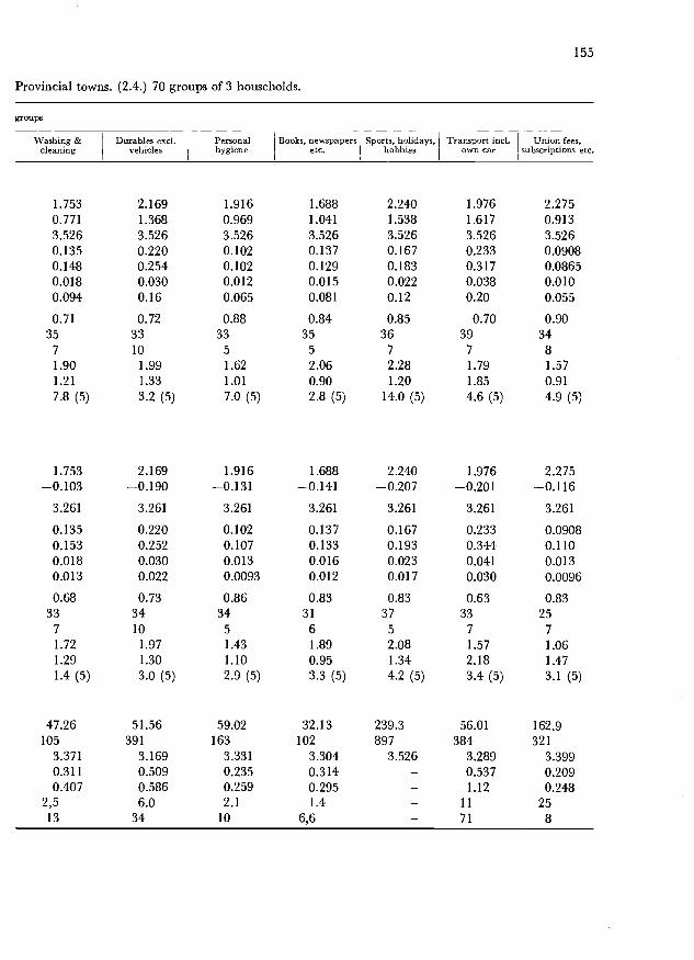
Provincial towns. (2.4.) 70 groups of 3 households.

155

357

3310

335

355

367

397

348

1.90 1.99 1.62 2.06 2.28 1.79 1.571.21 1.33 1.01 0.90 1.20 1.85 0.917.8 (5) 3.2 (5) 7.0 (5) 2.8 (5) 14.0 (5) 4.6 (5) 4.9 (5)

1.753 2.169 1.916 1.688 2.240 1.976 2.275-0.103 -0.190 -0.131 -0.141 -0.207 -0.201 -0.116

3.261 3.261 3.261 3.261 3.261 3.261 3.261

0.135 0.220 0.102 0.137 0.167 0.233 0.09080.153 0.252 0.107 0.133 0.193 0.344 0.1100.018 0.030 0.013 0.016 0.023 0.041 0.0130.013 0.022 0.0093 0.012 0.017 0.030 0.0096

0.68 0.73 0.86 0.83 0.83 0.63 0.8333

7

1.721.291.4 (5)

47.26105

34101.971.303.0 (5)

51.56391

3451.431.102.9

59.02163

(5)

31

61.890.953.3 (5)

32.13102

3752.081.344.2

239.3897

(5)

3371.572.183.4

56.01384

(5)

2571.061.473.1

162.9321

(5)

groups

Washing &cleaning

Durables excl.vehicles

Personalhygiene

Books, newspapersetc.

Sports, holidays,hobbies

Transport incl.own car

Union fees,subscriptions etc.

1.753 2.169 1.916 1.688 2.240 1.976 2.2750.771 1.368 0.969 1.041 1.538 1,617 0.9133.526 3.526 3.526 3.526 3.526 3.526 3.5260.135 0.220 0.102 0.137 0.167 0.233 0.09080.148 0.254 0.102 0.129 0.183 0.317 0.08650.018 0.030 0.012 0.015 0.022 0.038 0.0100.094 0.16 0.065 0.081 0.12 0.20 0.055

0.71 0.72 0.88 0.84 0.85 0.70 0.90

3.371 3.169 3.331 3.304 3.526 3.289 3.3990.311 0.509 0.235 0.314 - 0.537 0.2090.407 0.586 0.259 0.295 - 1.12 0.248

2,5 6.0 2.1 1.4 - 11 2513 34 10 6,6 - 71 8

156

Appendix A. Main results (continued). Unskilled workers.

log y = log k + log 1' (a + log x)

RN1

dFx2 (f)

1400

0.6532

61.801.384.55 (7)

230

0.5332

7

1.821.124.19 (7)

1800

0.8934

91.880.804.87 (7)

27000

0.7944

52.450.858.51 (7)

10000

0.7638

7

2.571.795.25 (7)

210

0.684562.291.421.81 (7)

Parameter estimatesand test results

Expenditure

Dwelling Fuel & light Food Tobacco Clothing Footwear

R 0.63 0.52 0.88 0.84 0.87 0.72N 36 30 29 41 34 451 6 10 9 6 9 5

d 1.71 1.53 1.61 2.03 2.21 2.04F 1.65 1.40 0.94 0.89 1.74 1.38

x2 (f) 12.9 (5) 12.0 (5) 1.5 (5) 3.8 (5) 9.0 (5) 4.7 (5)

4: y = a + b (X

a 318.8 225.0 1014 98.77 134.5 60.73b10 -70.2 -16.9 -140 -31.6 -55.5 -11.4

10 3.261 3.721 4.023 6.179 6.658 4.719X

- 0.238 0.151 0.422 0.284 0.251- 0.310 0.199 0.501 0.438 0.308- 8.5 25 7.6 10 2.4- 5.1 13 3.0 4.1 1.1

R 0.50 0.42 0.79 0.78 0.86 0.79N 28 21 27 31 31 371 7 16 10 8 11 6

d 1.57 1.37 1.00 1.35 1.86 1.94F - 1.70 1.73 1.41 2.38 1.50

x2 (f) - 11.8 (5) 4.6 (5) 18.3 (5) 8.0 (5) 5.8 (5)

a -4.667 -3.831 -4.422 -5.905 -5.513 -4.451k 2290 592.6 5920 19230 12270 410.7

0.122 0.103 0.0656 0.183 0.123 0.1090.143 0.109 0.0587 0.169 0.165 0.1300.41 0.41 0.23 0.56 0.38 0.38

Provincial towns. (2.4.) 70 groups of 3 households.

groups

157

0.7333

61.781.72

0.823110

1.741.33

0.9032

51.311.22

0.913561.820.88

0.782912

1.95-

0.552711

1.254.39

0.822581.051.40

11.1 (5) 10.4 (5) 7.9 (5) 3.9 (5) - 52.5 (5) 1.8 (5)

43.22 49.65 57.45 30.38 113.6 44.56 208.6-9.90 -33.9 -14.3 -8.91 -57.8 -45.4 -56.7

5.271 7.420 5.527 5.928 4.991 5.665 3.261

0.311 0.509 0.235 0.314 0.385 0.5370.489 0.694 0.349 0.377 0.649 1.362.9 7.2 2.8 1.7 11 12

1.2 3.4 1.1 0.67 7.1 9.3

0.71 0.77 0.84 0.85 0.71 0.52 0.78

1.961.207.45 (7)

2.051.302.23 (7)

1.690.981.94

--

(7) -

- - 0.09- - 20.71- - 34.51 (7)

32 21 21 27 27 23 2110 11 17 10 10 11 141.492.48

31.9 (5)

1.501.86

19.6 (5)

0.792.21

12.2 (5)

1.131.446.6 (5)

1.362.84

25.2 (5)

1.106.38

88.7 (5)

1.94

0.69 0.74 0.88 - - - 0.6235 33 33 - - - 19

7 10 5 - - - 20

-4.858 -6.414 -5.394 - - - -9.571628.2 77220 2714 - - - 1080-10e

0.135 0.220 0.102 - - - 0.09080.148 0.251 0.101 - - - 0.4140.45 0.66 0.32 - - - 0.028

460 150000 1800 - - - 100.108

Washing & Durables excl. Personal Books, newspapers Sports, holidays, Transport incl. Union fees,cleaning vehicles hygiene etc. hobbies own car subscriptions etc.

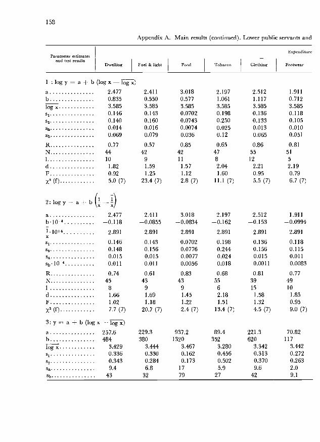
158

Appendix A. Main results (continued). Lower public servants and

dF

1.820.92

1.591.25

1.571.12

2.041.60

2.210.95

2.190.79

x2 (f) 5.0 (7) 23.4 (7) 2.8 (7) 11.1 (7) 5.5 (7) 6.7 (7)

2: log y = a + b -a 2.477 2.411 3.018 2.197 2.512 1.911

-0.118 -0.0855 -0.0834 -0.162 -0.153 -0.09941.10+4 2.891 2.891 2.891 2.891 2.891 2.891X

si 0.146 0.143 0.0702 0.198 0.136 0.1180.148 0.156 0.0776 0.244 0.156 0.1150.015 0.015 0.0077 0.024 0.015 0.0110.011 0.011 0.0056 0.018 0.0011 0.0083

R 0.74 0.61 0.83 0.68 0.81 0.77N 45 43 43 55 39 491 8 9 9 6 15 10

d 1.66 1.69 1.45 2.18 1.58 1.85F 1.02 1.18 1.22 1.51 1.32 0.95x2 (f) 7.7 (7) 20.7 (7) 2.4 (7) 13.4 (7) 4.5 (7) 9.0 (7)

3:y= a + b(logx-logx)a 257.6 229.3 937.2 89.4 221.3 70.82b 484 380 1320 352 620 117

log x 3.429 3.444 3.467 3.280 3.342 3.4420.336 0.330 0.162 0.456 0.313 0.2720.343 0.284 0.173 0.502 0.370 0.2639.4 6.8 17 5.9 9.6 2.0

sa 43 32 79 27 42 9.1

Parameter estimatesand test results

Expenditure

Dwelling Fuel & light Food Tobacco Clothing Footwear

log y = a + b (log x log x)

a 2.477 2.411 3.018 2.197 2.512 1.911b 0.835 0.550 0.577 1.061 1.117 0.712log x 3.585 3.585 3.585 3.585 3.585 3.585s1 0.146 0.143 0.0702 0.198 0.136 0.118

0.140 0.160 0.0743 0.250 0.133 0.1050.014 0.016 0.0074 0.025 0.013 0.0100.069 0.079 0.036 0.12 0.065 0.051

R 0.77 0.57 0.85 0.65 0.86 0.81N 44 42 42 47 55 51

10 9 lI 8 12 5

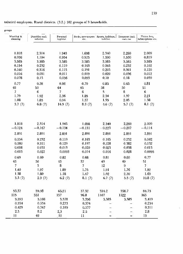
salaried employees. Rural districts. (3.2.) 102 groups of 3 households.

48 50 64 45 58 50 517 6 7 6 5 8 6

159

1.79 1.92 2.36 1.85 2.34 1.97 2.211.08 1.85 0.94 1.37 1.55 2.05 1.383.7 (7) 6.8 (7) 14.9 (7) 8.3 (7) 4.6 (7) 5.7 (7) 8.1 (7)

1.818 2.314 1.943 1.698 2.340 2.260 2.009-0.124 -0.167 -0.134 -0.131 -0.223 -0.207 -0.114

2.891 2.891 2.891 2.891 2.891 2.891 2.891

0.154 0.232 0.119 0.163 0.165 0.252 0.1020.180 0.311 0.129 0.197 0.228 0.382 0.1320.018 0.031 0.013 0.020 0.023 0.038 0.0130.013 0.022 0.0093 0.014 0.016 0.028 0.0095

0.69 0.60 0.82 0.68 0.81 0.60 0.7743

7

1.401.383.5 (7)

53.37115

5051.971.802.9 (7)

59.98551

4381.891.186.2

65.21157

(7)

377

1.751.478.1 (7)

37.3296.8

4912

1.911.926.7

314.21107

(7)

4991.762.305.5

358.71522

(7)

517

1.821.69

10.8 (7)

84.73165

groups

Washing &cleaning

Durables excl.vehicles

Personalhygiene

Books, newspapersetc.

Sports, holidays,hobbies

Transport incl.own car

Union fees,subscriptions etc.

1.818 2.314 1.943 1.698 2.340 2.260 2.0090.936 1.104 0.954 0.925 1.590 1.530 0.8193.585 3.585 3.585 3.585 3.585 3.585 3.5850.154 0.232 0.119 0.163 0.165 0.252 0.1020.160 0.316 0.115 0.191 0.205 0.361 0.1200.016 0.031 0.011 0.019 0.020 0.036 0.0120.078 0.15 0.056 0.093 0.10 0.18 0.059

0.77 0.58 0.86 0.70 0.85 0.65 0.81

3.393 3.166 3.378 3.356 3.585 3.585 3.4190.354 0.534 0.273 0.374 - - 0.2340.429 0.747 0.319 0.577 - - 0.3112.5 8.2 2,3 2.5 - - 2.8

11 49 10 11 - - 13

160

Appendix A. Main results (continued). Lower public servants and

5: log y = log k + log '1 (a + log x)

Parameter estimatesand test results

Expenditure

Dwelling Fuel & light Food Tobacco Clothing Footwear

R 0.74 0.77 0.86 0.81 0.83 0.79N 43 47 42 52 29 491 8 9 9 6 15 10

d 1.60 1.60 1.57 2.08 1.46 1.96F 1.04 0.74 1.15 1.21 1.39 0.94

x2 (f) 9.5 (7) 8.1 (7) 8.9 (7) 12.5 (7) 19.4 (7) 13.9 (7)

4: y = a + b (

a 275.0 230.9 962.7 204.0 226.1 74.86bl0 -46.5 -38.3 -136 -64.1 -59.2 -11.9

ak

-5.0754481

-4.2741067

-4.3464738

-5.6798851

-9.573l573l0

-4.734660.3

s1 0.146 0.143 0.0702 0.198 0.136 0.1180.139 0.157 0.0726 0.247 0.369 0.1100.37 0.40 0.19 0.47 0.038 0.31

2900 510 1100 9500 220l0 310

R 0.76 0.74 0.86 0.76 0.61 0.81N 44 42 44 51 31 491 10 9 10 8 17 9d 1.90 1.63 1.65 2.09 0.30 2.20F 0.91 1.21 1.07 1.55 7.35 0.79

z2 (f) 2.89 (9) 20.85 (9) 8.98 (9) 11.00 (9) 34.47 (9) 4.92 (9)

l0-- 4.109 4.179 3.797 2.891 5.379 3.943X

s1 0.336 0.330 0.162 - 0.313 0.272s2 0.407 0.330 0.2 16 - 0.473 0.324sa 12 8.0 21 - 13 2.5

5.3 3.6 11 - 5.0 1.2

R 0.66 0.73 0.79 0.74 0.76 0.71N 35 33 33 53 23 431 14 19 23 8 24 14

d 1.22 1.41 1.08 2.14 0.91 1.41F 1.47 1.00 1.79 - 2.28 1.42

x2 (f) 14.1 (7) 14.7 (7) 14.8 (7) - 47.1 (7) 22.1 (7)

salaried employees. Rural districts. (3.2.) 102 groups of 3 households.

groups

161

0.99 1.82 1.45 2.01 1.23 1.78 1.542.15 2.14 - - - - -

36.8 (7) 47.0 (7) - - - -

1300 20000 1500 960 - 230.108 620

1.721.108.81 (9)

2.051.827.93 (9)

2.360.93

13.83 (9)

1.861.368.91 (9)

- 1.52- 2.64- 3.78 (9)

2.221.38

11.22 (9)

0.7241

7

1.421.47

14.0 (7)

56.40-11.5

0.764411

1.941.96

38.8 (7)

33.37-51.3

0.843715

1.791.36

18.6

100.6-28.9

(7)

0.683512

1.842.38

43.2 (7)

61.7-18.7

0.773916

1.91

--

314.2-137

0.4537142.18

--

358.7-174

0.7951

7

1.951.76

11.5

114.2-28.7

(7)

37 41 33 35 33 27 3910 11 15 13 15 14 14

0.73 0.58 0.86 0.71 - 0.30 0.8047 52 62 42 - 42 53

7 5 7 6 - 11 6

-5.340 -5.790 -5.395 -5.317 - -9.377 -5.0301688 15290 2538 1219 - 409.8.108 1397

0.154 0.232 0.119 0.163 - 0.252 0.1020.162 0.313 0.115 0.190 - 0.410 0.1200.38 0.55 0.29 0.40 - 0.13 0.26

4.578 7.814 2.891 2.891 2.891 2.891 2.891

0.354 0.534 - - -0.519 0.780 - .- -3.2 6.3 - - -1.3 4.3 - - -0.66 0.76 0.79 0.67 0.74 0.46 0.86

Washing & Durables excl. Personal Books, newspapers Sports, holidays, Transport incl. Union fees,cleaning vehicles hygiene etc. hobbies Own car subscriptions etc.

162

Appendix A. Main results (continued). Skilled workers.

ExpenditureParameter estimates

and test results

R 0.81 0.45 0.92 0.70 0.82 0.69N 25 19 29 21 22 28

7 10 6 6 5 5

Dwelling Fuel & light Food Tobacco Clothing Footwear

log y = a + b (log x log x)

a 2.409 2.336 2.982 2.168 2.366 1.769

b 0.926 0.322 0.649 0.933 1.021 0.617log x 3.488 3.488 3.488 3.488 3.488 3.488

s1 0.126 0.105 0.0481 0.185 0.134 0.129

s2 0.123 0.120 0.0520 0.166 0.134 0.1220.017 0.017 0.0073 0.023 0.019 0.0170.095 0.091 0.040 0.14 0.10 0.093

dFx2 (f)

1.650.950.6 (3)

1.431.302.3 (3)

2.031.179.4 (3)

2.120.815.9 (3)

1.950.993.0 (3)

1.940.898.6 (3)

-2.409 2.336 2.982 2.168 2.366 1.769

-0.126 -0.0565 -0.0870 -0.118 -0.141 -0.0843

3.523 3.523 3.523 3.523 3.523 3.523

0.126 0.105 0.0481 0.185 0.134 0.1290.120 0.111 0.0618 0.173 0.137 0.1240.017 0.016 0.0087 0.024 0.019 0.0170.013 0.012 0.0066 0.019 0.015 0.013

0.82 0.57 0.88 0.67 0.81 0.6825

5

1.720.914.1 (3)

2010

1.671.112.9 (3)

2561.321.662.2 (3)

2551.950.873.7 (3)

2541.841.056.2 (3)

2851.860.923.7 (3)

- log x)207.1 211.2 870.1 128.8 187.5 55.23555 254 1450 331 526 88.6

3.349 3.426 3.404 3.364 3.354 3.4070.291 0.243 0.111 0.425 0.309 0.2980.293 0.247 0.128 0.420 0.283 0.2639.3 7.5 16 8.3 8.1 2.1

57 45 100 53 51 13

log y = a + b (

ab101 . .X

s2

Sa

sylO4RN

dFX2 (f)

y = a + b (log xab

s,s2

Sa

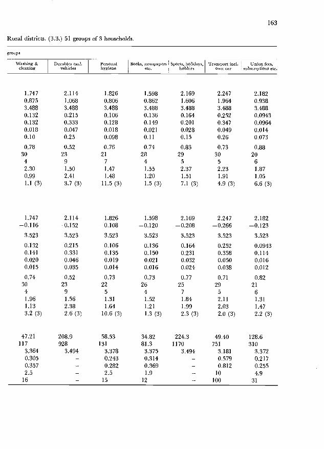
Rural districts. (3.3.) 51 groups of 3 households.

163

304

239

217

284

295

305

206

2.30 1.50 1.47 1.55 2.37 2.23 1.870.99 2.41 1.48 1.20 1.51 1.91 1.051.1 (3) 3.7 (3) 11.5 (3) 1.5 (3) 7.1 (3) 4.9 (3) 6.6 (3)

1.747 2.114 1.826 1.598 2.169 2.247 2.182-0.116 -0.152 -0.108 -0.120 -0.208 -0.266 -0.123

3.523 3.523 3.523 3.523 3.523 3.523 3.523

0.132 0.215 0.106 0.136 0.164 0.252 0.09430.141 0.331 0.135 0.150 0.231 0.358 0.1140.020 0.046 0.019 0.021 0.032 0.050 0.0160.015 0.035 0.014 0.016 0.024 0.038 0.012

0.74 0.52 0.73 0.73 0.77 0.71 0.823041.961.13

2391.562.38

2251.311.64

2641.521.21

257

1.841.99

2952.112.03

21

61.311.47

3.2 (3) 2.6 (3) 10.6 (3) 1.3 (3) 2.3 (3) 2.0 (3) 2.2 (3)

47.21 208.9 58.53 34.82 224.3 49.40 128.6117 928 131 81.3 1170 751 310

3.364 3.494 3.378 3.375 3.494 3.181 3.3720.305 - 0.243 0.314 - 0.579 0.2170.357 - 0.282 0.369 - 0.812 0.2552.5 - 2.5 1.9 - 10 4.9

16 - 15 12 - 100 31

groups

Washing &cleaning

Durables excl.vehicles

Personalhygiene

Books, newspapersetc.

Sports, holidays,hobbies

Transport incl.own car

Union fees,subscriptions etc.

1.747 2.114 1.826 1.598 2.169 2.247 2.1820.875 1.068 0.806 0.862 1.606 1.964 0.9383.488 3.488 3.488 3.488 3.488 3.488 3.4880.132 0.215 0.106 0.136 0.164 0.252 0.09430.132 0.333 0.128 0.149 0.201 0.347 0.09640.018 0.047 0.018 0.021 0.028 0.049 0.0140.10 0.25 0.098 0.11 0.15 0.26 0.073

0.78 0.52 0.76 0.74 0.83 0.73 0.88

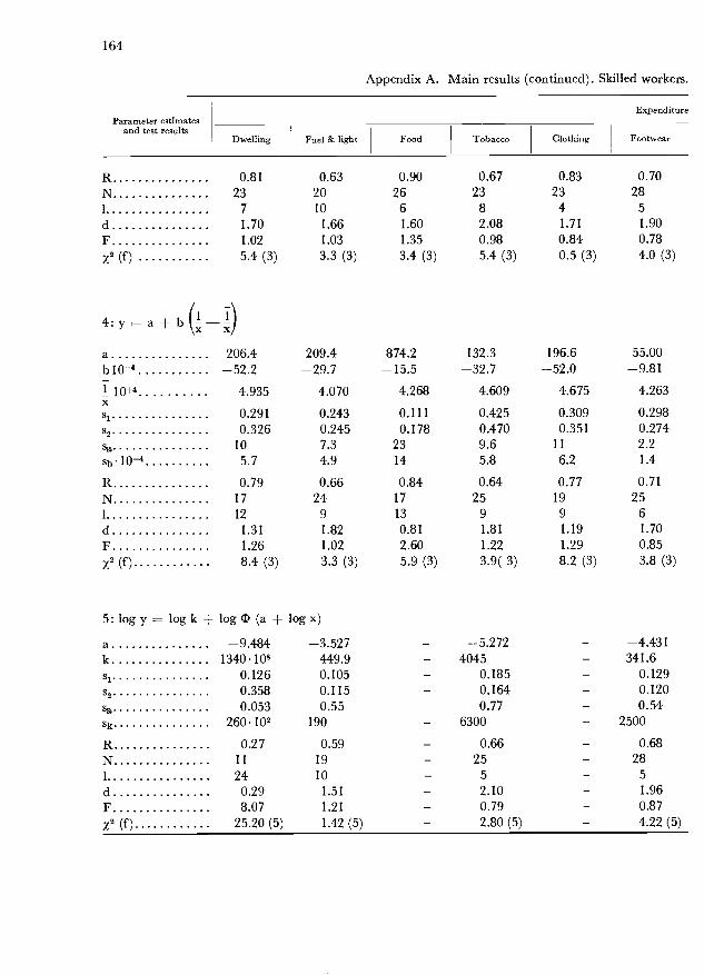
164

Appendix A. Main results (continued). Skilled workers.

ExpenditureParameter estimates

and test results

5: log y = log k + log D (a + log x)

Dwelling Fuel & light Food Tobacco Clothing Footwear

RN

dF

0.8123

7

1.701.02

0.632010

1.661.03

0.9026

61.601.35

0.6723

82.080.98

0.8323

41.710.84

0.7028

51.900.78

x2 (f) 5.4 (3) 3.3 (3) 3.4 (3) 5.4 (3) 0.5 (3) 4.0 (3)

4: y = a + b (

a 206.4 209.4 874.2 132.3 196.6 55.00b10-4 -52.2 -29.7 -15.5 -32.7 -52.0 -9.81

I 10+ 4.935 4.070 4.268 4.609 4.675 4.263X

si 0.291 0.243 0.111 0.425 0.309 0.2980.326 0.245 0.178 0.470 0.351 0.274

sa 10 7.3 23 9.6 11 2.2

SbiO4 5.7 4.9 14 5.8 6.2 1.4

R 0.79 0.66 0.84 0.64 0.77 0.71

N 17 24 17 25 19 251 12 9 13 9 9 6

d 1.31 1.82 0.81 1.81 1.19 1.70

F 1.26 1.02 2.60 1.22 1.29 0.85(f) 8.4 (3) 3.3 (3) 5.9 (3) 3.9( 3) 8.2 (3) 3.8 (3)

ak

-9.484134010

-3.527449.9

- -5.272- 4045

- -4.431- 341.6

s1 0.126 0.105 - 0.185 - 0.129s2 0.358 0.115 - 0.164 - 0.120

0.053 0.55 - 0.77 - 0.54Sk 260.102 190 - 6300 - 2500

R 0.27 0.59 - 0.66 - 0.68N 11 19 - 25 - 281 24 10 - 5 - 5

d 0.29 1.51 - 2.10 - 1.96F 8.07 1.21 - 0.79 - 0.87

z2 (f) 25.20 (5) 1.42 (5) - 2.80 (5) - 4.22 (5)

Rural districts. (3.3.) 51 groups of 3 households.

groups

Washing &cleaning

Durables excl.vehicles

Personalhygiene

Books, newspapersetc.

Sports, holidays,hobbies

Transport incl.Own car

Union fees,subscriptions etc.

165

0.76 0.59 0.78 0.21 0.56 - 0.8630 23 21 15 27 - 224 9 7 14 7 - 62.290.992.51 (5)

1.522.333.16 (5)

1.441.445.95 (5)

0.278.37

23.25 (5)

1.462.588.84 (5)

- 1.83- 1.06- 2.36 (5)

0.73264

0.2117

9

0.7822

5

0.6924

8

0.4113

16

0.73239

0.82196

1.94 2.54 1.24 1.53 2.35 1.45 1.221.37 - 1.34 1.39 - 1.96 1.387.0 (3) - 4.5 (3) 4.8 (3) - 4.1 (3) 1.5 (3)

50.09 109.5 59.15 35.22 224.3 52.37 129.9-12.1 -37.1 -13.5 -7.60 -133 -72.4 -29.6

4.496 5.628 4.530 4.622 3.479 6.782 4.675

0.305 0.494 0.243 0.314 - 0.579 0.2170.452 1.21 0.343 0.401 - 1.02 0.3513.5 20 3.0 2.1 - 15 6.82.1 11 1.8 1.2 - 12 4.0

0.65 0.42 0.73 0.66 0.50 0.65 0.7217 15 21 24 15 21 15

7 11 6 8 16 12 15

-5.151 -5.664 -4.963 -9.510 -9.384 - -5.3181161 8798 959.2 220.3.108 548.108 - 4529

0.132 0.215 0.106 0.136 0.164 - 0.09430.131 0.327 0.127 0.394 0.263 - 0.09710.51 0.80 0.41 0.054 0.099 - 0.36

1100 16000 700 42.108 230.108 - 3300

1.51 1.17 0.85 1.35 2.19 0.91 0.722.20 6.03 1.99 1.63 - 3.10 2.61

19.3 (3) 52.0 (3) 6.4 (3) 10.0 (3) - 5.5 (3) 11.0 (3)

166

Appendix A. Main results (continued). Unskilled workers.

ExpenditureParameter estimates

and test resultsDwelling Fuel & light Food Tobacco Clothing Footwear

log y = a + b (log x - log x)a.blog x

2

Sb

RN 44 391 5 10

d 1.91 1.54F 1.31 1.04

x2 (f) 3.8 (7) 17.7 (7)

2: log y = a + b (X X

a 2.321 2.336b104 -0.112 -0.0795

3: y = a + b (log x - log x)a 163.1 184.7b 416 350

1 . 10 3.788 3.788X

s1 0.133 0.114s2 0.164 0.110

0.017 0.011

5b 10 0.0097 0.0065

R 0.77 0.79N 35 401 11 14

d 1.66 1.71F 1.51 0.93x2 (f) 7.4 (7) 8.2 (7)

2.321 2.336 2.984 2.121 2.366 1.7430.981 0.642 0.665 1.275 0.993 0.4983.468 3.468 3.468 3.468 3.468 3.4680.133 0.114 0.0565 0.169 0.112 0.1120.152 0.116 0.0520 0.187 0.136 0.1250.016 0.012 0.0054 0.019 0.014 0.0130.076 0.058 0.026 0.093 0.068 0.063

0.80 0.76 0.94 0.82 0.84 0.6446

649

646

6

478

1.74 2.28 2.43 2.170.85 1.22 1.47 1.259.0 (7) 11.7 (7) 3.6 (7) 8.9 (7)

2.984 2.121 2.366 1.743-0.0768 -0.145 -0.111 -0.0565

3.788 3.788 3.788 3.788

0.0565 0.169 0.112 0.1120.0619 0.202 0.153 0.1290.0064 0.021 0.016 0.0130.0037 0.012 0.0091 0.0077

0.91 0.78 0.79 0.613591.231.20

51

8

1.951.43

457

1.911.85

478

2.031.33

2.9 (7) 10.6 (7) 1.5 (7) 11.7 (7)

827.9 172.9 173.7 52.661420 531 461 65.7

3.336 3.468 3.269 3.3700.130 - 0.259 0.2580.126 - 0.367 0.260

11 - 7.5 1.558 - 37 7.4

s1

3.2810.306

3.3240.262

s2 0.385 0.2497.3 5.1

Sb 36 26

Rural districts. (3.4.) 93 groups of 3 households.

groups

167

469

456

51

847

651

649

9366

1.93 1.76 1.96 1.79 2.02 1.85 1.860.91 1.75 0.94 0.96 1.23 1.54 0.799.0 (7) 7.3 (7) 3.8 (7) 5.2 (7) 5.2 (7) 4.0 (7) 10.6 (7)

1.696 2.068 1.775 1.556 2.073 2.057 2.180-0.0993 -0.104 -0.0990 -0.107 -0.179 -0.174 -0.108

3.788 3.788 3.788 3.788 3.788 3.788 3.788

0.136 0.207 0.108 0.146 0.173 0.236 0.08570.144 0.264 0.118 0.146 0.214 0.336 0.09110.015 0.027 0.012 0.015 0.022 0.035 0.00950.0086 0.016 0.0070 0.0087 0.013 0.020 0.0054

0.77 0.57 0.83 0.79 0.83 0.67 0.9039

944

7

4010

406

456

3910

376

1.55 1.90 1.49 1.69 1.60 1.42 1.341.13 1.61 1.20 1.01 1.53 2.02 1.13

10.5 (7) 7.8 (7) 14.1 (7) 8.8 (7) 4.9 (7) 4.5 (7) 9.4 (7)

39.87 89.28 46.16 27.16 33.27 219.7 114.592.5 279 110 71.5 322 1060 282

3.295 3.246 3.290 3.274 3.090 3.468 3.2870.313 0.477 0.248 0.335 0.398 - 0.1970.344 0.636 0.268 0.358 0.634 - 0.2 181.6 7.0 1.4 1.1 3.8 - 2.97.8 35 7.1 5.7 26 - 14

Washing & Durables excl. Personalcleaning vehicles hygiene

Books, newspapersetc.

Sports, holidays,hobbies

Transport incl.own car

Union fees,subscriptions etc.

1.696 2.068 1.775 1.556 2.073 2.057 2.1800.888 0.791 0.872 0.914 1.571 1.659 0.9353.468 3.468 3.468 3.468 3.468 3.468 3.4680.136 0.207 0.108 0.146 0.173 0.236 0.08570.129 0.275 0.104 0.143 0.192 0.294 0.07600.013 0.028 0.011 0.015 0.020 0.030 0.00790.065 0.14 0.052 0.071 0.096 0.15 0.038

0.82 0.52 0.87 0.80 0.86 0.76 0.93

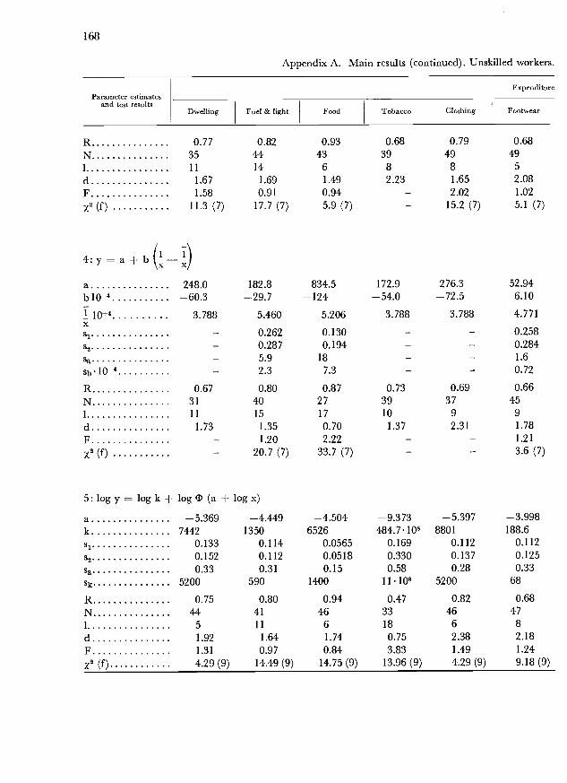
168

Appendix A. Main results (continued). Unskilled workers.

log y = log k + log 1) (a + log x)

Parameter estimatesand test results

Expenditure

Dwelling Fuel & light Food Tobacco Clothing Footwear

R 0.77 0.82 0.93 0.68 0.79 0.68N 35 44 43 39 49 491 11 14 6 8 8 5

d 1.67 1.69 1.49 2.23 1.65 2.08F 1.58 0.91 0.94 - 2.02 1.02

x2 (f) 11.3 (7) 17.7 (7) 5.9 (7) - 15.2 (7) 5.1 (7)

4: y = a + b ( -a 248.0 182.8 834.5 172.9 276.3 52.94bl04 -60.3 -29.7 -124 -54.0 -72.5 -6.10

I 10 3.788 5.460 5.206 3.788 3.788 4.771X

s1 - 0.262 0.130 - - 0.258- 0.287 0.194 - - 0.284- 5.9 18 - - 1.6

s 10 - 2.3 7.3 - - 0.72

R 0.67 0.80 0.87 0.73 0.69 0.66N 31 40 27 39 37 451 11 15 17 10 9 9

d 1.73 1.35 0.70 1.37 2.31 1.78

F - 1.20 2.22 - - 1.21

x2 (f) - 20.7 (7) 33.7 (7) - - 3.6 (7)

RN1

dFx2 (f)

0.7544

51.921.31

4.29 (9)

0.804111

1.640.97

14.49 (9)

0.9446

61.740.84

14.75 (9)

0.473318

0.753.83

13.96 (9)

0.8246

6

2.381.494.29 (9)

0.6847

82.181.249.18 (9)

a -5.369 -4.449 -4.504 -9.373 -5.397 -3.998k. 7442 1350 6526 484.7.108 8801 188.6

1 0.133 0.114 0.0565 0.169 0.112 0.112

0.152 0.112 0.0518 0.330 0.137 0.1250.33 0.31 0.15 0.58 0.28 0.33

5200 590 1400 11.108 5200 68

Rural districts. (3.4.) 93 groups of 3 households.

groups

670 1400 580 620 11010

0.79 0.59 0.86 0.82 0.58

169

1.07 1.78 0.90 1.28 1.38 2.27 1.661.82 - 2.09 1.70 - - -

42.1 (7) - 30.6 (7) 28.1 (7) -

1.880.918.19 (9)

1.801.707.93 (9)

1.950.945.01 (9)

1.820.94

11.25 (9)

0.982.52

11.29 (9)

0.7835

91.581.21

0.6642

7

1.971.77

0.864481.511.17

0.8242

7

1.641.14

0.8131

14

0.972.53

0.1617

201.62

-

0.903561.291.22

31.4 (7) 26.2 (7) 27.4 (7) 13.9 (7) 35.7 (7) - 12.7 (7)

41.69 152.7 45.17 26.93 175.9 219.7 169.9-7.63 -33.7 -9.03 -5.62 -68.7 -99.9 -40.1

5.619 3.788 6.025 6.204 3.788 3.788 3.788

0.313 - 0.248 0.3350.422 - 0.358 0.4362.0 - 1.9 1.40.78 - 0.71 0.51

0.73 0.68 0.80 0.75 0.52 0.45 0.8831 42 31 35 27 19 2913 7 12 14 14 22 15

48 45 47 49 339 6 8 6 19

-5.118 -4.876 -5.077 -5.195 -9.3061022 1497 1127 868.9 327.710

0.136 0.207 0.108 0.146 0.1730.130 0.270 0.105 0.141 0.2750.34 0.54 0.27 0.37 0.075

Washing & Durables excl. Personal Books, newspapers Sports, holidays, Transport incl. Union fees,cleaning vehicles hygiene etc. hobbies own car subscriptions etc.

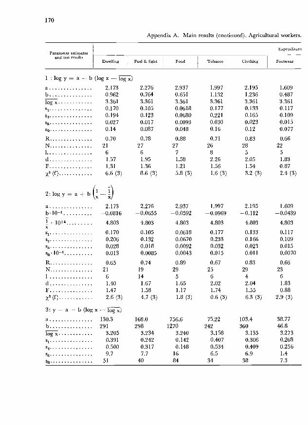
170

Appendix A. Main results (continued). Agricultural workers.

ExpenditureParameter estimates

and test resultsDwelling Fuel & light Food Tobacco Clothing Footwear

log y = a + b (log x - i)ablog x

s2

s

RN1

dFx2 (f)

2: log y = a + b (

ab1041 . 10X

s

RN1

dFx2 (f)

3: y = a + b (log xablog xsis2

s

21

6276

277

268

285

225

1.57 1.95 1.58 2.26 2.05 1.831.31 1.36 1.21 1.56 1.54 0.876.6 (3) 8.6 (3) 5.8 (3) 1.6 (3) 3.2 (3) 2.4 (3)

2.173 2.276 2.937 1.997 2.195 1.609-0.0816 -0.0655 -0.0592 -0.0969 -0.112 -0.0439

4.803 4.803 4.803 4.803 4.803 4.803

0.170 0.105 0.0618 0.177 0.133 0.1170.206 0.132 0.0670 0.233 0.166 0.1090.028 0.018 0.0092 0.032 0.023 0.0150.013 0.0085 0.0043 0.015 0.011 0.0070

0.65 0.74 0.89 0.67 0.83 0.66

2.173 2.276 2.937 1.997 2.195 1.6090.962 0.764 0.651 1.132 1.236 0.4873.361 3.361 3.361 3.361 3.361 3.3610.170 0.105 0.0618 0.177 0.133 0.1170.194 0.123 0.0680 0.221 0.165 0.1090.027 0.017 0.0093 0.030 0.023 0.0150.14 0.087 0.048 0.16 0.12 0.077

0.70 0.78 0.88 0.71 0.83 0.66

216

19

1429

5

256

294

236

1.40 1.67 1.65 2.02 2.04 1.831.47 1.58 1.17 1.74 1.55 0.882.6 (3) 4.7 (3) 1.8 (3) 0.6 (3) 6.3 (3) 2.9 (3)

- log x)130.3 168.0 756.6 75.22 103.4 38.77291 298 1270 242 360 46.8

3.205 3.234 3.240 3.158 3.135 3.2730.391 0.242 0.142 0.407 0.306 0.2680.500 0.3 17 0.148 0.534 0.409 0.2569.7 7.7 16 6.5 6.9 1.4

51 40 84 34 38 7.3

Rural districts. (3.5.) 53 groups of 3 households.

171

238

305

326

314

227

256

226

1.43 2.33 1.78 1.52 1.34 1.83 1.852.07 1.39 0.94 1.54 1.54 2.20 1.278.8 (3) 1.3 (3) 5.6 (3) 6.1 (3) 1.8 (3) 9.7 (3) 3.5 (3)

1.660 1.953 1.655 1.464 1.900 1.846 2.080-0.0634 -0.0823 -0.0656 -0.106 -0.118 -0.0677 -0.0782

4.803 4.803 4.803 4.803 4.803 4.803 4.803

0.132 0.220 0.109 0.153 0.191 0.208 0.1150.214 0.252 0.106 0.172 0.265 0.327 0.1330.029 0.035 0.015 0.024 0.036 0.045 0.0180.014 0.016 0.0068 0.011 0.017 0.021 0.0085

0.54 0.58 0.80 0.80 0.70 0.41 0.7923

6

354

247

286

247

238

254

1.15 2.50 1.72 1.90 1.07 1.66 1.752.65 1.31 0.95 1.25 1.91 2.47 1.331.7(3) 1.1 (3) 5.3 (3) 3.3 (3) 6.6 (3) 8.1 (3) 3.4 (3)

43.69 72.85 38.63 14.84 37.47 76.44 93.5883.5 210 74.6 74.7 244 136 2373.237 3.169 3.224 3.092 3.062 3.214 3.1880.303 0.507 0.251 0.354 0.441 0.479 0.2650.546 0.564 0.251 0.380 0.776 0.894 0.3003.5 6.4 1.4 1.0 5.7 9.7 4.3

18 34 7.4 6.0 36 51 22

groups

Washing &cleaning

Durables excl.vehicles

Personalhygiene

Books, newspapersetc.

Sports, holidays,hobbies

Transport incl.own car

Union fees,subscriptions etc.

1.660 1.953 1.655 1.464 1.900 1.846 2.0800.865 0.847 0.727 1.096 1.429 0.922 0.8753.361 3.361 3.361 3.361 3.361 3.361 3.3610.132 0.220 0.109 0.153 0.191 0.208 0.1150.189 0.260 0.105 0.191 0.237 0.309 0.1300.026 0.036 0.014 0.026 0.033 0.042 0.0180.13 0.18 0.075 0.13 0.17 0.22 0.092

0.67 0.54 0.81 0.75 0.77 0.51 0.80

172

Appendix A. Main results (continued). Agricultural workers.

5: log y = log k + log I (a + log x)

Parameter estimatesand test results

Expenditure

Dwelling Fuel & light Food Tobacco Clothing Footwear

R 0.63 0.72 0.90 0.71 0.80 0.67N 23 21 31 25 27 221 7 19 5 6 7 6d 1.60 1.82 1.68 2.02 1.90 1.88F 1.63 1.72 1.09 1.72 1.78 0.91

(f) 4.9 (3) 20.2 (3) 0.8 (3) 3.2 (3) 2.1 (3) 8.5 (3)

4:y= a+ b(_)a 128.8 169.3 759.5 75.24 192.6 39.22b10 -20.6 -21.3 -90.3 -15.6 -41.8 -3.39

ak

-5.1934530

-4.6571965

-4.3235381

-5.6358802

-5.90328920

-3.849131.7

si 0.170 0.105 0.0618 0.177 0.133 0.1170.193 0.122 0.0651 0.220 0.162 0.1080.60 0.39 0.24 0.60 0.45 0.49

5600 1200 1800 13000 34000 68

R 0.59 0.71 0.90 0.70 0.82 0.67N 21 27 29 28 28 221 6 6 5 4 5 5

d 1.56 1.94 1.69 2.25 2.15 1.89

F 12.9 1.35 1.11 1.54 1.49 0.85

z2 (f) 2.90 (5) 10.64 (5) 3.69 (5) 0.05 (5) 3.16 (5) 4.00 (5)

I 10+ 7.083 6.497 6.400 7.905 4.803 5.840X

s1 0.391 0.242 0.142 0.407 - 0.268s2 0.529 0.344 0.180 0.611 - 0.269sa 10 8.5 20 7.4 - 1.5

3.5 3.0 7.1 2.5 - 0.57

R 0.64 0.71 0.87 0.66 0.72 0.64N 23 17 23 21 23 21

1 9 19 10 10 7 6d 1.39 1.47 1.20 1.65 1.94 1.73

F 1.83 2.02 1.60 2.25 - 1.00

x2 (f) 3.3 (3) 3.2 (3) 8.3 (3) 2.9 (3) - 7.0 (3)

Rural districts. (3.5.) 53 groups of 3 households.

groups

173

680 2100 250 2500 - 2400 1700

45.74 72.83 39.47 12.30 28.90 84.90 94.73-579 -14.0 -5.15 4.84 -16.6 -10.3 -16.1

6.339 7.524 6.558 9.269 9.861 6.176 7.203

0.303 0.507 0.251 0.354 0.441 0.479 0.2650.646 0.580 0.299 0.400 0.986 0.998 0.3664.3 6.7 1.7 1.0 6.6 12 5.31.6 2.2 0.61 0.37 2.8 4.6 1.8

0.46 0.66 0.76 0.88 0.64 0.29 0.78

0.5223

81.372.144.91 (5)

0.6030

5

23.71.331.98 (5)

0.8332

61.830.90

13.66 (5)

0.8431

41.691.396.66 (5)

- 0.34- 25- 6- 1.88- 2.21- 10.29 (5)

0.822441.861.243.03 (5)

21 33 16 27 17 17 238 4 19 8 7 12 8

0.53 0.66 0.82 0.90 0.71 0.37 0.8323 31 26 28 18 21 25

8 4 7 8 7 9 41.17 2.23 1.73 1.99 0.76 1.67 1.81

3.24 1.24 1.00 1.15 3.10 3.49 1.28

3.2 (3) 2.7 (3) 3.6 (3) 4.0 (3) 29.5 (3) 34.4 (3) 3.2 (3)

1.00 2.12 1.37 1.85 0.49 1.47 1.444.53 1.31 1.43 1.28 4.99 4.34 1.90

10.0 (3) 5.1 (3) 9.3 (3) 2.4 (3) 45.4 (3) 44.3 (3) 13.1 (3)

-4.918 -4.898 -4.562 -5.549 - -5.072 -4.964778.2 1467 399.4 2066 - 1638 2244

0.132 0.220 0.109 0.153 - 0.208 0.1150.193 0.254 0.103 0.180 - 0.309 0.1280.47 0.79 0.41 0.53 - 0.74 0.41

Washing & Durables excl. Personal Books, newspapers Sports, holidays, Transport incl. Union fees,cleaning vehicles hygiene etc. hobbies own car subscriptions etc.

174

Appendix B.

The tables show the correlation coefficient') between the residuals of the differentexpenditure items, where the calculated expenditures are calculated from the functionlog y = a + b (log x - log x). The tables are shown separately for each of the twelvegroups of wage and salary earners cf. the heads of the tables.

The numbers 1-13 in the head and the front column of the tables denote the differentexpenditure items according to the following code:

Dwelling.Full and light.Food.Tobacco.Clothing.Footwear.Washing and cleaning.Durables (excl, own car).Personal hygiene.Books, newspapers etc.Sports, holidays, hobbies.Transport incl, own car.Union fees, subscriptions etc.

) Cf. chapter VI, p. 105.

1.1 Higher public servants and salaried employees. The capital.

1 2 3 4 5 6 7 8 9 10 11 12 13

- 0.309 0.076 0.045 -0.093 -0.043 0.161 0.176 0.067 -0.096 0.023 0.057 -0.1002 - - 0.017 -0.053 -0.240 -0.081 -0.002 0.099 -0.145 -0.181 -0.385 -0.060 -0.1563 - - - 0.288 0.290 0.102 0.365 -0.045 0.145 -0.032 0.176 0.004 0.0334 - - - - 0.163 0.055 0.176 -0.116 0.233 0.160 0.122 0.032 -0.1565 - - - - - 0.578 0.319 -0.052 0.485 0.141 0.359 0.003 0.1006 - - - - - - 0.191 0.060 0.432 0.116 0.127 -0.114 -0.0227 - - - - - - - -0.011 0.338 0.020 0.258 -0.027 0.0778 - - - - - - - - 0.017 -0.139 -0.030 -0.043 0.041g - - - - - - - - - 0.381 0.342 -0.028 0.044

10 - - - - - - - - - - 0.378 0.053 0.08111 - - - - - - - - - - - 0.065 0.14112 - - - - - - - - - - - - 0.08013 - - - - - - - - - - - - -

1.2 Lower public servants and salaried employees. The capital.

1 2 3 4 5 6 7 8 9 10 11 12 13

1 - 0.395 0.082 -0.055 -0.046 0.122 0.154 0.039 0.02 1 0 077 0.074 -0.028 0.0212 - - 0.076 -0.055 -0.125 -0.075 0.073 -0.016 -0.139 0.014 -0.144 -0.070 0.0063 - - - 0.262 0.013 0.004 0.204 0.048 0.053 0.166 0.073 -0.061 0.1524 - - - - 0.013 -0.064 0.128 -0.011 0.042 0.158 0.067 0.102 0.1875 - - - - - 0.469 0.199 0.099 0.365 0.124 0.302 -0.046 0.0216 - - - - - - 0.132 0.148 0.370 0.078 0.172 -0.073 -0.0067 - - - - - - - 0.043 0.235 0.114 0.185 0.095 0.0558 - - - - - - - - 0.094 0.146 -0.024 -0.054 0.1229 - - - - - - - - - 0.222 0.207 -0.041 0.061

10 - - - - - - - - - - 0.109 -0.116 0.34711 - - - - - - - - - - - 0.051 0.00412 - - - - - - - - - - - - 0.08213 - - - - - - - - - - - - -

1.3 Skilled workers. The capital.

1 2 3 4 5 6 7 8 9 10 11 12 13

1 - 0.369 -0.117 0.003 -0.324 -0.283 -0.046 0.054 -0.047 0.155 0.025 0.017 0.162

2 - - 0.110 -0.057 -0.185 -0.146 -0.126 0.015 -0.038 0.205 -0.066 -0.124 0.2253 - - - -0.017 -0.193 -0.037 0.267 -0.165 0.065 0.079 0.048 -0.340 0.1974 - - - - -0.127 -0.089 0.244 0.085 0.120 0.034 0.171 -0.185 -0.0315 - - - - - 0.480 -0.176 0.112 0.265 0.061 0.110 0.010 -0.2076 - - - - - - -0.132 0.056 0.120 -0.077 0.074 -0.077 -0.1227 - - - - - - - -0.055 0.018 0.099 0.204 -0.035 0.0868 - - - - - - - - 0.076 0.152 0.109 -0.182 -0.0399 - - - - - - - - - 0.173 0.116 0.018 -0.055

10 - - - - - - - - - - 0.165 -0.110 0.06411 - - - - - - - - - - - -0.219 -0.22712 - - - - - - - - - - - - -0.09713 - - - - - - - - - - - - -

1.4 Unskilled workers. The capital.

1 2 3 4 5 6 7 8 9 10 11 12 13

1 - 0.336 -0.097 0.024 0.161 0.122 0.151 0.067 0.169 0.074 0.034 -0.167 -0.0162 - - -0.166 -0.034 -0.171 -0.123 -0.073 0.133 0.079 -0.031 -0.049 0.020 0.127

3 - - - 0.133 0.025 -0.086 0.265 -0.143 0.014 0.114 0.049 -0.032 0.186

4 - - - - -0.100 -0.030 0.186 -0.104 0.025 0.069 0.024 0.041 0.129

5 - - - - - 0.532 0.172 0.196 0.338 0.126 0.182 -0.187 0.034

6 - - - - - - 0.265 0.099 0.300 0.053 0.092 -0.032 -0.0667 - - - - - - - -0.034 0.121 0.180 -0.049 -0.026 -0.0298 - - - - - - - - 0.111 -0.023 -0.053 -0.161 0.040

9 - - - - - - - - - 0.110 0.083 -0.012 0.114

10 - - - - - - - - - - 0.102 -0.171 0.190

11 - - - - - - - - - - - -0.164 0.186

12 - - - - - - - - - - - - -0.01613 - - - - - - - - - - - - -

2.1 Higher public servants and salaried employees. Provincial towns.

1 2 3 4 5 6 7 8 9 10 11 12 13

- 0.294 0.129 0.076 -0.052 -0.102 0.119 0.115 0.054 0.114 -0.053 -0.122 0.2402 - - 0.338 -0.026 -0.192 -0.131 0.050 -0.075 -0.182 0.044 -0.078 -0.086 0.0473 - - - 0.016 -0.235 -0.200 0.087 -0.108 -0.071 -0.039 -0.206 -0.093 0.1354 - - - - 0.282 0.088 0.307 -0.095 0.368 0.072 0.288 -0.070 0.2435 - - - - - 0.469 0.252 0.130 0.507 0.121 0.237 -0.062 0.0876 - - - - - - 0.060 0.001 0.423 0.078 0.268 -0.115 -0.0507 - - - - - - - -0.048 0.366 0.2 14 0.032 -0.093 0.37 1

8 - - - - - - - - -0.024 -0.096 -0.130 -0.122 -0.0729 - - - - - - - - - 0.210 0.323 -0.114 0.311

10 - - - - - - - - - - 0.282 -0.162 0.06611 - - - - - - - - - - - -0.182 0.06612 - - - - - - - - - - - --0.04913

2.2 Lower public servants and salaried employees. Provincial towns.

1 2 3 4 5 6 7 8 9 10 11 12 13

1 - 0.250 0.001 0.023 -0.066 -0.109 0.124 -0.010 -0.101 -0.130 -0.160 -0.054 -0.0072 - - 0.127 -0.040 -0.252 -0.223 0.029 -0.075 -0.252 -0.045 -0.165 -0.167 0.1133 - - - 0.009 -0.045 0.073 0.028 -0.132 -0.090 -0.076 -0.117 -0.112 0.1594 - - - - 0.018 -0.053 0.204 -0.094 -0.026 0.084 0.191 -0.055 0.1295 - - - - - 0.510 0.080 0.020 0.390 0.065 0.111 -0.075 0.0266 - - - - - - 0.024 -0.008 0.397 0.167 0.138 -0.042 0.0287 - - - - - - - -0.044 0.098 0.157 0.104 0.014 0.0198 - - - - - - - - 0.052 0.002 - 0.116 -0.042 -0.1079 - - - - - - - - - 0.162 0.172 -0.029 -0.050

10 - - - - - - - - - - 0.182 -0.032 0.07811 - - - - - - - - - - - -0.148 0.05812 - - - - - - - - - - - - -0.13913 - - - - - - - - - - - - -

2.3 Skilled workers. Provincial towns.

2.4 Unskilled workers. Provincial towns.

2 3 4 5 6 7 8 9 10 11 12 13

- 0.278 0.026 -0.032 0.046 -0.104 -0.013 -0.064 0.000 -0.089 -0.013 0.062 -0.0342 - - 0.149 -0.135 -0.125 -0.109 -0.202 0.097 0.128 0.216 -0.274 -0.129 0.1353 - - - -0.077 0.061 0.024 -0.034 -0.236 -0.035 0.239 -0.101 -0.138 0.2884 - - - - -0.034 0.097 0.293 -0.038 -0.009 0.085 0.255 -0.158 0.0935 - - - - - 0.596 0 179 0.191 0.136 0.000 0.191 -0.396 -0.1236 - - - - - - 0.122 0.174 0.148 0.144 0.127 -0.336 -0.0487 - - - - - - - -0.098 0.156 0.061 0.467 -0.070 0.1308 - - - - - - - - 0.164 0.004 -0.141 -0.224 -0.2429 - - - - - - - - - 0.309 0.086 -0.045 0.028

10 - - - - - - - - - - 0.014 -0.223 0.25111 - - - - - - - - - - - -0.186 0.26912 - - - - - - - - - - - - -0.09113

2 3 4 5 6 7 8 9 10 11 12 13

- 0.292 -0.065 -0.104 -0.066 -0.119 0.120 -0.122 0.012 -0.075 -0.035 -0.232 0.0362 - - 0.217 0.009 -00l3 -0.059 0.099 -0.040 -0.128 0.105 -0.174 -0.288 0.1083 - - - 0.042 -0.388 -0.327 -0.111 -0.183 -0.326 0.193 -0.209 -0.208 0.2604 - - - - -0.032 -0.078 0.073 -0.135 0.017 0.211 -0.063 0.009 0.061

5 - - - - - 0.590 0.445 0.086 0.373 0.028 -0.006 -0.135 -0.1986 - - - - - - 0.307 0,088 0.394 0.019 0.149 -0.109 -0.1157 - - - - - - - -0.088 0.482 0.137 -0.096 -0.196 0.0678 - - - - - - - - 0.015 -0.174 -0.101 -0.191 -0.0179 - - - - - - - - - 0.073 0.101 -0.081 -0.200

10 - - - - - - - - - - 0.085 -0.151 0.09911 - - - - - - - - - - - 0.411 -0.04312 - - - - - - - - - - - - -0.01113

3.2 Lower public servants and salaried employees. Rural districts.

3.3 Skilled workers. Rural districts.

1 2 3 4 5 6 7 8 9 10 11 12 13

- 0.183 0.036 -0.005 -0.112 -0.079 -0.044 -0.199 -0.037 -0.112 -0.114 -0.061 -0.0112 - - -0.024 -0.099 -0.222 -0.227 -0.123 -0.087 -0.248 0.011 -0.263 -0.186 -0.0243 - - - 0.046 0.001 -0.042 -0.016 -0.014 -0.047 0.085 0.124 0.037 -0.1724 - - - - 0.157 0.028 0.195 0.010 0.192 0.017 0.315 -0.066 0.0605 - - - - - 0.428 0.152 0.251 0.359 0.042 0.090 -0.068 0.0696 - - - - - - 0.220 0.092 0.360 0.041 0.032 -0.032 -0.0567 - - - - - - - -0.044 0.291 0.171 -0.152 0.038 0.1108 - - - - - - - - 0.097 -0.076 -0.004 -0.149 -0.0119 - - - - - - - - - 0.085 0.178 -0.071 -0.111

10 - - - - - - - - - - -0.081 0.130 0.05211 - - - - - - - - - - - -0.022 -0.18012 - - - - - - - - - - - - -0.02113 - - - - - - - - - - - - -

1 2 3 4 5 6 7 8 9 10 11 12 13

I - 0.341 0.005 0.021 -0.097 -0.205 0.109 -0.102 -0.004 0.062 -0.149 -0.167 0.0352 - - 0.093 0.254 0.036 -0.144 0.087 -0.197 -0.154 0.251 -0.224 0.002 0.0143 - - - 0.231 0.145 -0.118 0.196 -0.327 -0.035 0.009 -0.096 -0.301 0.3144 - - - - 0.092 0.040 0.251 -0.234 -0.015 0.230 -0.010 -0.207 0.1655 - - - - - 0.496 0.429 -0.292 0.082 0.057 0.084 -0.124 -0.0256 - - - - - - 0.052 -0.098 0.255 0.104 0.216 0.068 -0.0257 - - - - - - - -0.274 0.384 0.058 0.198 -0.305 0.0278 - - - - - - - - -0.229 -0.188 -0.054 -0.265 -0.2709 - - - - - - - - - 0.276 0.199 0.024 0.103

10. - - - - - - - - - - 0.087 -0.017 0.07611 - - - - - - - - - - - 0.136 0.04112 - - - - - - - - - - - - -0.09513 - - - - - - - - - - - - -

3.4 Unskilled workers. Rural districts.

1 2 3 4 5 6 7 8 9 10 11 12 13

- 0.191 -0.174 -0.067 -0.109 0.013 -0.125 -0.083 0.075 0.066 -0.132 0.122 0.036

2 - - 0.108 -0.253 -0.097 -0.027 0.080 0.095 -0.146 0.296 -0.447 -0.033 -0.0113 - - - -0.018 0.040 -0.101 0.165 -0.134 0.017 -0.058 -0.048 -0.173 0.060

4 - - - - -0.020 0.003 0.163 -0.045 0.228 0.098 0.052 0.020 0.083

5 - - - - - 0.447 0.043 0.096 0.398 -0.006 0.224 -0.062 -0.2306 - - - - - - 0.147 0.065 0.402 0.066 0.254 0.036 -0.0667 - - - - - - - 0.026 0.152 0.090 0.193 -0.004 0.210

8 - - - - - - - - 0.240 0.103 -0.057 -0.158 -0.1759 - - - - - - - - - 0.087 0.216 -0.074 -0.083

10 - - - - - - - - - - -0.091 0.096 0.149

11 - - - - - - - - - - - -0.003 0.007

12 - - - - - - - - - - - - 0.092

13 - - - - - - - - - - - - -

3.5 Agricultural workers. Rural districts.

1 2 3 4 5 6 7 8 9 10 11 12 13

1 - 0.491 -0.190 0.031 0.051 0.015 0.116 -0.076 0.076 -0.062 -0.233 -0.079 -0.0842 - - 0.056 -0.050 0.014 -0.146 0.127 -0.123 -0.090 0.250 -0.228 -0.092 0.136

3 - - - -0.060 0.046 -0.136 0.003 -0.186 -0.153 0.220 0.120 -0.165 0.045

4 - - - - 0.055 -0.052 0.222 -0.124 0.220 0.060 0.015 0.073 -0.0135 - - - - - 0.458 -0.061 0.170 0.299 -0.041 0.025 -0.195 -0.1626 - - - - - - 0.035 0.134 0.149 -0.070 0.165 -0.117 -0.1247 - - - - - - - -0.214 -0.013 0.262 0.333 0.322 0.990

8 - - - - - - - - 0.290 -0.115 -0.245 0.070 -0.0969 - - - - - - - - - -0.080 -0.048 -0.104 -0.026

10 - - - - - - - - - - -0.101 -0.030 0.240

il - - - - - - - - - - - -0.008 0.123

12 - - - - - - - - - - - - -0.00913 - - - - - - - - - - - - -

181

Appendix C. The basic material.

Disposable income, expenditures on 13 items, savings, assets and some other informationseparately for each of 3098 households of wage and salary earners in the year 1955.

All amounts are in Danish kroner, (respectively 100 Danish kroner). The amountsgiven in columns 3-16 are in kroner per person, all other informations are per household.The columns l-22 contains the following information separately for each household.

Column Informationno.

1 Household number within the socialgroup in question.

2 Size of household measured in number of persons.

3 Disposable income per person of the household (i.e. total money income less paid personaltaxes).

4 Expenditure per person on dwelling.

5 Expenditure per person on fuel and light.

6 Expenditure per person on food.

7 Expenditure per person on tobacco.

8 Expenditure per person on clothing.

9 Expenditure per person on footwear.

10 Expenditure per person on washing and cleaning.

Il Expenditure per person on durables (excl. own car).

12 Expenditure per person on personal hygiene.

13 Expenditure per person on books, newspapers, etc.

14 Expenditure per person on sports, holidays, hobbies.

15 Expenditure per person on transport (incl, own car).

16 Expenditure per person on union fees, subscriptions, etc.

17 Savings (net changes in assests and debts).

18 Income changes in the period 1953-55 according to the following code:Rising through the whole period 1953 / 1954 / 1955.Constant - - - - 1953 = 1954 = 1955.Decreasing - - - 1953 \ 1954 \ 1955.Unknown 1953-1954, rising 1954-1955.Unknown 1953-1954, constant 1954-1955.Unknown 1953-1954, decreasing 1954-1955.

9. No information.

19 Type of household according to the following code:Single men.Single women.

182

Couples without children.Couples with one child.Couples with two children.Couples with three children.Couples with four or more children.Single men with one child or more.Single women with one child or more.

O. Other types of household.

20 Net assets in 100 kr.

21 Wage- and salary income in per cent of total income.

22 Year of establishment of the household (60 denotes no information).

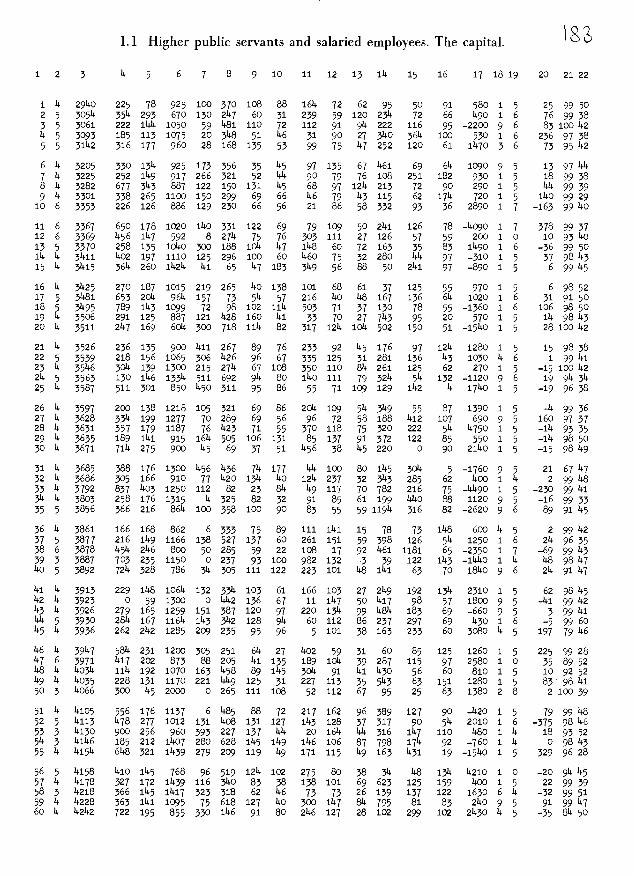
I1!dqj s Aojdm p.nps pu SjUAJS ijqnd JqIj

çîOsjZç6ot

æt.g

66ztg

Z0T9Zç6L19

LZT9tiZLi1Tooç

09169liT0çç6TZZLOtiLZT9T9Lç6oTTs1Tç9ç

ZsZ1l9i

1109s16ç

î9 O9TZZTLT6cT9ZLL91Z98TÇÇLT11T5îT99ç9TZ5îççT00116TZTZ969TOt 9T99O19tt 6çTzLtL9L111iLOOTZsîs1Çtgtj1ç9ç09LZZOTsjat6Tç9699!çs110Th9ÇTIIç9ç

çTOit- 61TÇI1ç9T6sçtTLT6116116oZ6LZ6çslT1ZÇ919h1çT11

11t09LZ6slLt96LL99019tit611TshiT9Z9o9LotitZTZ9T91111111ç

s091jOTTL11T9t1111si9TOZ11t1LtLZZ0969çZ 006oçTl1c9tOTOZ506LTçLç9ZTçs1TLZITTScsitçTZtotLLZ9L11dth çToZsj-06LZt69d96Z91LIZZL819LdTT9LT90Tiî11t9ZO9çtç9çz6L9ZTTZ901TTTç9ZO000ZÇs1ood99011çoçç09Z1TtÇ9ç11çççdTTLzz1çZT6iTZZOLTTTdt9ZZçç011sj6sçT0TS099çoç11111t6oçç11t6ggçd9TOLotZ6tTT11dOti11811oTOgçZL61tL9Z6dhot69T15joZ99dLgZOZLT11TL69LsçO9Ztç909t6çZOLZ1191Z ç0çOOZT TZ s1gçL116d11911

ç11080ç09ççZç91gçTOTç96ç6çç6oZç9ZTZ5jZZ9Z9d6çç19T0ç1169L6ZLZ 99ZTT091169ZTZ1jdç11t11911L9T118Zoç6çç11ï

6099-69çgt9sI66ijÇtOZZL6oZtLgç TT 6ztç916)39Z6ç11ç11

ç6008TL96p1oL11TL99çtZtTil00ç16çodZ6d11Z11çToTZ11çtZ6T611ZLzçot99T19doT11ççZdT11901911T6ZZç16çs1111

96O+9TOLç9Tslt911TOtZZZZ1ITTç0çijd99LgZd11ZLZ69Çc011

11tO1tTçsiTZZT6dçZ960016LdzooçtTçççoLqçç6dLToççz-ç91811t911Z6LT901ZZ6ç9Zoç g11ç11gLgd9TOZT11ç9Z186ç6çt19Z09LdTLZ9dT991T611T91ZLL8dçççsloo9L9Lçt1111ItT68ç!ççç9Z9999T99199ç119ç

960Z9ZZ99Td1161T 6çççç806OOTgççOOT119891Z99ç9ç9ççççç6OZTT99ot11166TT9ç816ZdZ9ççTT 9LtgçZço9ç11t1çIO6trtl-L9TZZ9LOLLIT611119dZZ9ZTToçZTç011LdgZ6Lcsçç1110011Z9ç9Zdt1çZçLÇZ11ZToçTOZLLoT6991çoc989ç11Zd ç6o9LT-çj10çç11109OCTiLLTtiL9119ç11ooçT9LTggçç99ç11Td

çO11TZ060OZZç11gç9ç11TçL69ç11006LZsltLTL9dhççççgZZTZLç16LT ç9TT 901 çç119T16p11691çç9ç116ZçToçL1111çZZZoZdçLoçççTLçZ119!L9TT6LTççTç9ç118Zç6069LOTZ11198T9çZL969ç6969zOLLLZT66Thc9Z9ççTo6çtL9çç6s1c11ç6othioZ9969 lZççoTg1ZTgçTooZL6ç119Z

çIoslLt11Z11T6ZT60TILçç986Tt0ç110ç9oç11çL996OZTT- ZT11ç

11Zd6LTTT011Tog116Z69tt11ççt911TOdTç9ççç11ZçOLZZ9çZTT9Z5j9Ott0ççSOTL911LZTZ ooct 6Ts10ç911çç11dZ911odolç119çTt9ZtZTçççL9969Z5j9odç9Ot9çTSTZççççZZçTO9ZT11Z1L69Ltç11Z6çç9!69L9Zt111006çç19dZ9ZççsjTZ

çTo11çt-ço1Zot11Z1itçZ91ITT9TLoo1i0969TL11ZlTççsiOZçToLOZ6çL LZo!ççT110919Z11TZTL88ZTt6Z90çç11619to9ç-çç9LoTLILçoçTTZot96ZL6601ç11t6gLÇ6s1Çç91

tOZOT1199çTL9191iosi91Zç11ççLT 11961-oZçç9T911ççLIçToL6ççZ1Ld1999tOTgçtOsç9Z6TZTOTLgT0LZçZ11çî9T

ç1069-L6T11Z0ç9ç611çd9TL11ç911111Z11T09Z119çTt1Tç1çToTd-L61111OSZZdç!09110900196ZZTOTTtL6tZ011TTç11siT

9To611tçgççd9TZL099111L11t1OT891oodOlOTçç19çZoLçççdTOTooZ6çL9ZTLZTITdod9LçjsiLZ8Z6L11T9ç1169çç9ZtL106011-gL9ZT1hZ0ç6016L69ZZ1Idd0111oæt 9LT0ç9L9çç9TT

L1o6gZ9çç6çç9ç99TZ9çOdZ6Z19999ZT9ZZçççç9OTçtOZ!tiLlZ9ç11d116!911996966ZoçtOOTTç9Z9ççTodc116

Io6Z06ZLçTZ11ZTL689ç11TçT0çTZZTL99cçLL9Z9Zd119çToc6Z91T?9019L6L061111ZçTZd99?LT66111ZZçç11L

ç6o6oT11969t911L9çç1ç11çç9çççLIçZ611çloççoZ119

ç0L11T19OZTZZLs1ç!66çççç19919Z096LLT9TdZ111dççtoçç001119fot1ÇLZ06Tç911T911dOZçLoTdITçgIç6oçç11

96ooZZ-69tTZZZ11616ZtTZ!OTTT8IT6çoçolttTZZZT90dçç9To61199ZLI1ÇZOZT6ç6cZtd09L11Z0çT0L9ç6Z11çç11ç0çççT09çT6oç6?9?L119T99oLc oatZ69!cz0116Z11T

6T 9TLI91çT11tdTZTTT0169L9çiçZT

O5j9-L5î66T6

66ZÇ666ZZçs1 116OZ-

ç966Zç1g60Zç Ç6T

95j g6çLç-9i 666L

6d 001 Z11196çgZçZ6O1

69çç9Z 66çZZ

911 6LL6109 66ç-T5T 66çZ11 66111-ç11 96Z9

Ls1 t611Z

L11 8691ç11 6669-çç 9611Z

Z1166Z

ç11 166gçç 6691-T11 66OçZ-91i66ZL11 L9TZ

611g6çT-oç 9611T-çç6111-Lç L60919ç66tr-gç 966T-11ç 1166TZ11 OOT ç1-11166Tgç 96çT

Z11001 8Zç11 g6hT0ç 969010ç T6çZç 969

ç11 6691196Lç

oç 669ç-os1 ç6oTLç 669LÇ

o66ç9t-6Z 6601116Ç66i-tgç 669111L6ç1

Z116dLgç L69çZ11 001 ç8gç669Lo66çZ

ZZ IZOZ

Çt Ç6ÇÇTOt11-OT9tOTTOTt1619îTLi6T691 OT oz6TiiÇ90toT0609t?9iOTT9t?TTLLTT69L1t69TTL6669t111-tflç6TTL6LLTT06TÇ6T9ÇOTÇ90T oLi8T99T996oi1oÇt9T1

L6T0L9TÇTTÇT9TT6i 6T OTL 9T 69TÇ91Çco11LTT86Tot6c61cç811L9601OT99OT L9 Oo9T 999920Ç9TT

9Ç 66119-iT 09Tt?TTT9Ç18L19T696990ToSLoT999tTTOTT

9t?69oIe-ot1o6TT11T99ÇTL999LÇi1Ç12tTt-t996i111ITT*Ç6Ç6 0996o06t?9L966T*Lo9ÇÇtI9TT0Tt96t1t1TT

9OL09T099T991Toet1LeiiL99t?6TÇÇ9t?96t?11TT66To6Ç-11TL6*919T9t96999T O9T696t1Ç

09 001 L9-Ç9oi6oLi 66!TOijiT996ooL1 ooL9cÇ6i1OTTL6-*T0t909T69LTI96Ot?686OTTT9ÇÇ6o

6T6T0T6î909T9tT19OT11T199TLTToT901L16i-To*oÇT0109oT9TL9LT90tT9O1tj9Ti'6t?ÇLOTL669T-T0TT6î99T6Ç9698160t?1166îTfOT11TTTLj6t190T

c ooi T9T096eÇTL6T99ÇLÇ!T 6LTLTT OT o6oOT9IÇo6*tt?66ToT69861t?T6tÇî19t?ÇTT6oT0Too6t?oT

Tg6o6o6TLTOt?T99!69!Çt69TÇ9O0t1t?ÇcoT096L!909-0TT9TT 9611TILT9121 L9 69T ÇTT9tT9911ÇOT9Ç 96i9TO9-T9t9Tt?9T 6TT 99Ç996T9TTL9169O91TO

Ot?L6T0T999T90!9T09LT 0TT9T0TLtLt?Ç6L9it?OOT

911 66t?otjÇ9118T9619i1LOTT9L99111T96T6iL91166L69LOijT16ÇiTTTÇT LT9ÇT6Ç!fjOTÇT99t?t186

96T9tioÇT-TL6T91ÇÇ11LT9T9T 96tTTi1iÇÇLtIgt1L6669Ç6 oÇ69oL919991Ç9T 99oo6O6LLi1t196

L6LLioT6- TTLoTÇT69ijT90011Ot11*6T9LL11Ç

6T 9!TL1oo6i9999699L9*9961i oi oÇÇi9996t1ÇLLI1t1166i 9611ÇioLLe-OTL9LTLLLOTt106ocLTi9LToTLLtc6

COT o116000- 811ZOTTTIEt?TOO991.9LOTÇtoioiÇÇ)i1Ç666Lc-9ToLOTCoil099LTT96g090*TT9T69LÇL11cT6

6T0991T9oiTLL99it1LL1i6O10TOOTO9OLt106661iT-910t?T9TL*OÇ0999luiT9LL09OOliT619LÇÇ99j169

911 96LoTÇT011L9699LgL9999*69T 9LTT9T99i1199969L11OT0TOLL9TLcILTiT9996119TT 61OTT9t?L96h Ç6TITÇ*oI001*066661iOL9i

Çoo6æcT09t11199

T.Ç 96911*o9tT- LOTgLL9L66çI6ijiTOILL91T oL091T91 o*696006-6L6tLTt19T6T6ÇTOTTO0tIOÇTLTÇÇÇOL111ti9669ToT90TLL6i9T BOT9Tg6611999O9TT9Li1991

09 66TÇToi9T669TTÇ0T tÇ999Çi1

9i T6-6 oÇ-99ÇT ÇÇ 9T0TTiL6961tj*90T9T11T9

11 6699T-OTo6L9tjLT09TO18LT161oiTOOi612O9t909T96t1ÇTii oæ99961i6*9T99Ti11LTTÇ9ÇÇtÇ6L

L696-9TO1ît1T96TT1LLLT91!COT OOTt1i9L6TT olT-TLoTc96TO1j9oT6t1oT6cçoLL

TÇ 96Tt1ToLTOT9T9LL96!lOLOT9oLLoÇ96991111Ç9L

Lt?66Lt1i oTT- L1ii1cLT9Ç966TOPj9191TOT9Çt1tj19LLT11081-T969TT09T9ÇoÇLÇi19OÇ.T99T6oco66909TO6ÇT-0691199Ç3tOT11101001116Ç96).0OT L?290IÇi1i1cL

916O9*oLLÇ8Ç9TT9T6T cci 6L 0T T6LTcLi6TLi1OT099T-6iLTo1i166L9L919Çoi1118TL

tt L609-ÇT099Tt19LT9ILT69TT9t1i99T669TTot1ijOL96iI oLÇ9TIÇIOLLIToL6TiITTT9Li19Çi169

9Ç 669o6Ç9oÇ9t11L9!OTOt?99oo1 TT T1TLt999t? 661ÇTo69TLOI1198ÇÇ6969TITL9OLTT 9Tc OOT 6T6ocTTO01it1TITT Ç96066690T 66occc199

09 669T069tiLOTTLLL9TTO96T69TTT1TOi

t?669609T6oÇ9TIL9T6tT6OT9T6ooo6Çti119

Ifl T66tÇ11OTLi1TT996*oo6oOT9OÇÇiÇLoÇ1it1Ç99t1 001 9T-To66TÇÇÇTtiO8ïLT69Lcc oo6LTLotiOO1111

001 T-O091LT 9TL66o69Ç9L96TT991999i19

To6T 9TLT9TTtT1TTTOT68L9ÇtT

jtudiqj so1duj puqis pu SU1AJS qqndi

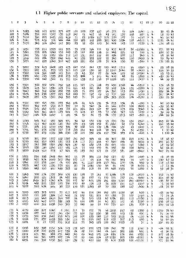
1uiidqj siojdui pnps put S1UAJS zqndiqij j

lit1 99LLT4100101901cocc91trÇ9ZT1ociL46c0?9469ZTZ6cTIL1Ç3911OIÇ66li6I111010?-6c149?6oI 91114196966ZLTtiltL8148Z1194199O39c6LI6c6LOTOIoÇ9iliii9L44Ç9 tn 401cc69c8t11461641L9Z0Z949L1

Ç 66Z-111o4t8199094i9911191.199t9644L991Z90?80?00?9CLLTT2611g-46090T6119L?iaolcLTo4491ZLI9L1i?Ç?44T86?c112619Z9L1

ÇÇ 46 9TÇTOL9?c6IIL1190014Z1Ç11Ç4LI1Z1646?L9411901919114LIÇ66?1110991ZLacZL9?oIL9?46?444T19ccc9IL4?IL?99191LIt111961191111OÇT-1199411Ç9LOIT21114T4019014Lti84?L911194?0cc64T94L109 664?IjT0096414914699404??IL001LLI0494111L9IIlilliL9994T9c?LI611 9L6441460441Z9LI??9?1 944LL4?6LII?1001001101Lo?61196Lo911TLT

cl Z666?4104?44109T6LLoIT1966911T4469469L9491114009oLo9?OLT1196 94?06064446L9I444119?98191194461?440001L6tiZT114?0946914c L6444410414OITOZ?11Ç?TLtic4T664?L116L0L04401111011111644109T991111 46Li.111o69TZ91OL049o610?1?4Z41IL9911L4i11941 æ1190T09cL9I6116699-41OLti969991491?11I4ti19L?911LoILT9LL0??I4?44?96664Ij991

04 9LtiT-4110011-LII811144LOL2941101IZI901?4404496tioti0T69L64t149101166460411LII0419L99LZIT9410904190L4?TL44146??911ti464c119TL? L9 4I111o6LoZ- 011?o6L469911116914Lti?1LIT664tiLtiO11LTL9c6111191164c491?4 9641?4104ti414T?IL19L61149L4I24601Lctiti6?0414?I96?Lti64i?9TLti 4LZ4I111oLo?-?01961t$?1 941tTLL9?10419L4004L4LItiL?004cti64191

14 9664Ij904?IOL49418Z1144691?42?TcZcÇÇtj006061c*?tT0624c091114 19L-ÇI0LI118L941181104164014L02491OL?cccIo6TL1cL9c6Ç1oT 46911116Octi11?I001111104?114?LIII144111061119964144?46991194494109 Lti04166oL4OLccco4LcÇo169011L9I611?L9c090?11L11LZti9Ç24cL4144 968-c100010111L9L?934?1416949L44L6tiIti?O11Tocc942I?9Ç?94T

49L9tiI01114-9?119494?18L?ILtiIc9149IZ11LI4L90T46Z4?O?94c4419? 1169114104911001399461964109TLL411T24LLT9111106134?9194111141911 669111101191L6109141908?91Z6LT ÇZi3i?16I99ÇLtTÇL194ÇL4 46I66 ooÇ19i490OLÇLII1111494cd19010I00969L411

Ld 8691tji0401ççLo46999iCLItiTL6oi ?91 L1 96I094L4

11d 001 1111009-90?489ÇLL4114? 841Idtodt1i1469416L?L9494LÇ041?11 66141ocdl-o1i6849016ocIIÇtiI9TLLZLLIdL1Z11ILti61114? 664T91OOIIT61944tj9 1I 6010?T01941164I60LTILl119?1ZL4c9111

t1 46961ÇIOtiltidT691I 19341 94Ç9c91011L0I 0011L11ÇLT9tTILÇ1111L6?tjT 093OdI1Ç9oL944601691?tj041L4d?4 L691tii1i19111

9Ç 66i1i1099-L3I99I LI8L1964ti461oLtTIIti1111Z01L9Ij4ti166664ti90L9116TL89L8L940149T9tc9I 0OI 46d90ti311

66111-1110114ç6oeLI0611LL9161?9? 40T101 4I L9tTT6oti 466C-IjI0?t9019L11tt1i119116011Ç?LocLd L130464616tÇo?4?t16h 66oIl41061-ti611ÇTÇ49t1411111119t1QT911d9? II 4tt064ooc4111111

646 o49T0812tOT9L6?49cIIÇ?9919Lo!666461130041LI98?961144otiL11116L14460914901664?LIcc69L61OL6111?TccLLcI9c3c11L114ti6I 11Ç 1166?41O9I903dIl964116L919L3IL4614L3636?T?4011dLtrtTÇ119c10?6?944ti09?-çdItidæ66111?I91116199L0c41old409ÇotÇ11LI6869L19Io1Ç4-*99L1OÇtjc20T4LIL314L1464?41d31440916494T

44 66ii1ÇToLtiIIII4I9311 OL941T?94141L41ooI3111991o64ti

6T 6664-lT09T19j00119114919OOIcL3?o3ÇÇ41d9ot69c4ccTotjo6Lo141111169L9?dÇ11Ç9o4c49189096ÇtiTI94LcdT

6d 66911Ç101116989ti9d091T L4960913014T199d4?TL9IT L9Z44It1?dI9? 86 d?i10689466ILI31ti63TL4II1941L11TL93T90111clti6LdL634çIcI

cc 001 IcI9TOoÇ-L90411111iOL99T949O?TLI109d011019099IL?4cOdT?11 6961160611?OI4011011c?L??Tccc4Ioi4oti9118?6I118e69969?ÇÇ 6T9t 16914iotjdLIT99?tj?949?1I91?141L91IL 6T ?8?6?Tc?cIti?4i2?T6d L699TIooL4Ç3d**99O1O31014?I999OÇ0iT40? 84I1ÇtL31cti 22IL?iI 0TI 98916tiLI1dlII1161?LI6L444IIIcccI6134L9d?Çc9I

869LTiI0L4??TI49T90ti9Ç0I1d9çL91011?T119oL14911 l91411ÇIoLc11-9ItÇ00611039??9136111119tt11190L6L11404ItiIctitZI

9611ti6o4T-9LLOIOL44oTLII6801Ç9IL6x11Ç9ÇiTI4oe96Ç91IÇdÇ?Tti 66tI o6911LI104cIlccLI1119LIIT9144T L94T99? 94toÇ4

tid 96?c41ot4II169ILcOLI601101Lo94LÇ o?T49T?9do4tiII

? I?oe6T 91LT91IIjiIZIII0169L9ÇdZI

21 L9 o49Ç6o6TL9tÇÇT669T 90TTLi9216hIT191LT2141L49904o?9L?090O? L69644606?460906TTTTL?1oL98?80TLo4Lo?218?449649909L?64?099049L4TOTL964LLT94496L4T69?tr?894949?T964L84LLI8429? 664?49o+L?6T99+6t?4L4240414601 ti9?9442Lo4969092144 9664904696?616TTT 44TTLI216Ltr901009990042 iÇ 6æT9TLL?94?

49 6664Ç60444-621?L949ÇT L9o046TT9i094OTIOO8Tt911?L9449L?44?96L008109090991181l9 9TT94TL99420426t494?T4TTT4o4ÇL49Lh94?69 001 ?TÇ1046T?40?211966194L69T?T?060T T?9OL9T944T9L429L44294 664?61001TTI09189444TT41LÇlITT600021L4246?T944gL9946??4?T? 66906Ç904?-?LT099106842T461to444860904??48TT11t1669?L4LT4?

9? 99TOT4To49- 99T9449906099?T?LT949L664ÇLr?o6T921942944L?04?9166 94T099ÇOTÇ?4T216T4294?942T44?T44oT 044094T90494L?4L6??9196T?4T000469T4oT4690649T884L44441214TL94?9T?4cL09L99L?80004 46814T040?OLT004?96OOT?91044æc 9042442000?490?4L49L?21?4 66I49OT?69144?L94OTTI99T900t0984r8?L9T8904TTT949L900

09 66T9441099LOT4619901 90146069LT6480414o9T0T94891?1LI44 66446OL?96146121990009?999166T46T46LTo?994T99009609L90094 6681-4T0090L9181T6641 091TILT190?19IL64449?0499LT442oLÇL?9? 069?99T021909T?00904L69694?9L164o649TLT46499021400?c4 96949019-9?4242014TÇ-r644 994426L9190060041964L49?942L

6? 9644?4TO?O?69?049T4889??ÇL444461 LL 44?944T944LT946?LI O?41 c6164IT09?9?90618L814LT8114616L84L9T4o404191?L46T?666991T069-64?462114OT 0964T9OT49TL94?? 64 449TT94gÇL4?L481?9? 66ÇÇT006149T9T?994ITT461T9?9606TOL0694?LT??4L6?961LLT

968169490919149TT69 96T4T844T4T6oTL49CII649L94994I6TL?9T?

494644T1T09T?90100?4L9444?6TITÇ44ÇTTT94O004T969441T9TL44T09 66?44o-i44T8418691 90T?9T 9164?8614LLo86?T4T4948OTLI9T44 001 0T60049??444O4T 4LT4?1Ç?0?Lo?1669T9 3O?421098?40LT4T?446!9999TO990T44T46941-ti9944T9?9?06994604L49TLT41499OL4

I? 69?CT49C??T0406684TT99119T49618T1T 411004T444LL449oL?TI?

9? 666T4TCOOT4?099001?OTTLT944L44210401 9400919L6?494069CT?t-t66o44TOT9T46OLT19I499O0099819419484L9419T6L4664L40L960??4 L944?16o66L4L001490T?09T6816914OTI49TO4TT4912186669490?9996969T009498044ÇÇOT 9T14L16ThOT?9T1940044T44I101?L69Loe49 L9094IT04044T4LT90?699646?TLTT9?6L14T46LT91198911TÇ69490?

T9 4694?1TOO?46I949TTOT 1994?96TO?4?T40118411L99469169440?69664TT49CO429?T?1I???9?O?14T994LT491844oL4T94?4L9T6914 9690T099499T6g460T 94O966LL9T9IT8LL994Ç4OTTTTL42016994o?4 4646o4oL991161T4OT 6L401964?T ?4T?49L6T42?T1414?4?699964 664911T04T9998T4T4L61T00942T69T404L6TIT944099?L99ÇTO?

44 66?t6O?IÇ44T9L040188400 T?99?669646TLL?TL9T?640999400?4? L6L9T0999944TLL9T 199694L144LT21144?T96T99?T8L9466T9966 464T046499ÇTT46L6T?44T41661211694??4OTT?4446469699gET09 96994909894419469L0819998619TT94TI?OO8T44246449L9?L6T94 L6L9T1606644T64906944?L98LT4o094LT44LToL4009LTL9496T

T? 969214T01900?L908T11 ?IITLO?LO?T4T901019?TT099T6?4L14TTL9?46T44 6644-1T0?904141?900T ?996L0T6LT?94LT OT ?4TT44?421999496T14 4640?9TO1-6oT991L944L46T000146648T?6414091T0000414999446TT96o?4TOI9T941001T9444T9?T064L9T89T214091429TT9?0041299?6T49 L60911T OLTV211099469??900o6T40141900909914

4? 4694?ÇIo6L191L9o1L?L42T6o99tL96649OT006199L690449?06T4 66491T00944TT00409664?8T491194444L9000TL6014699946814 66 4-6044199T?616?40644084T9T?O?I99T4T9L64?O9OT9699488T

4? 6664-Ç1O8118TTT4 61T9014?4OOT?499o644611904999T999?L9TI4 964-4TOI9ILTLT464L464OT? 9966919i T9T9?TT9L?L69T94998T

L169 ?T-9T01916g9L?9L4901ITTTOI666I44444091L9T4OT?94944g9T96901IT09699LT??99699TT691LIT?L091TL4960041?I?6T01494901146Ç490401-ÇITT6TI6014469T88161T91T109099L8ITÇÇT6L014949T

Ç 06ÇttoiL-88L8go44L4ÇÇ491TTLLtiLÇ6191?tl18?T69?949IÇÇ 68??9TO94TTT614LL?T LIOL9LLL8699T99?44TL6T86ÇÇ9g9ÇT8T

00T?O61 9TLT9T4TIT41TTTOT69L944T

I!dqjo1dmPn1pui 'IU1AJS Jflqndi j

9999TT09494T6T

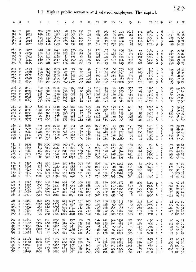
jiiidqj s'o1dui pups pu STUiAJS znqndj

44 OCT LT1109T3LT29IÇt1949T901911To4TOCT)26994029T9OoljT6iTTTootiÇ 469cÇTo3669363O0ÇÇ 201933lj6T94398f11891029TÇL3069T3TT66T4 OCT 119TT09909T9OÇT119Ç3 ooÇ0939Ç9934TÇ3Ç4J 04).0961Ç9096T96209 L6o2zTo1Ttz3Ç6L49z 34133oLO3TO9OT 8011066L6119111391TTTL6zÇ4 96LzÇTOÇIIT39TÇ9603 O9T4Ç LL49113).0ÇÇ4Ç ÇÇ 049T993962T1131113963

61196LLÇT049L09T494TL9T 40T9LTTt2tT92TTo64t90041L9LTIT9960Tz462T4 43eL-ÇT ooz9944t6toT 069348TLo1ÇÇ39LTT coL4TTÇoTt9TÇT499013163i666oiLTT4!otiz061939ÇOTLL60119096T92T11ÇToÇ90T6z12 Ç9 TÇ6TOC6112Tfl93L86L6zÇ9Ç92l9434LT9Ç9I1TÇ13tT0Ç99ÇTÇ990T2262L66oÇÇoOLTIIoo1L934T 119gT6TltjTIL09L621160433923T04049013162

09 001 0Tfl0023T9L924TT 003TL1iTTO9Ç96T9t9T 092T 00L234202).6T90TT063ot 662-ÇT0998T3QÇL9LT LÇ.230).89!63 T63T8TT 09119119TTL9T9T640T3692ti4 6639ÇT0992883ÇÇ9iÇI9619L3193293TTLT 6611t902031j9t96ÇoT2992T2 366LÇT01169-1j3209996O9314LTOCTÇ6t6094LL3oÇto63T99110T2L9209 OCT 9T-ÇT OT22T2Ç14TTooflL113003LÇTt69T Ç31169TÇ11019T9110T2993

6i 66231-Ç110861T11o6991 641169231t911963TL2T T1119032006Ç94oLoT392611693ÇToÇ9ÇÇÇ343Ç41829226319ÇT99!61366T6116113T1190013118303 994oToLLT11T333Ç9LT 04163T).Ç60T11o1193Ç4o6941L96L663Ç92L2 66193Ç

1106611j36T169T1 61TL936T99T921Ç949119oÇÇ369!00966329292 963ÇÇT0113T039LLLTT 903693IÇÇ99T99).19116961999 9TT11662T93

4 669-ÇTo6233TL6Ç49Çi633ÇÇTc2LT299LI40).o69T44Ç900T0L96309331 001 0ÇToÇÇoÇ61112 4139LToÇ61T4T6Ço1 941009T661 oÇ63Ç9636LLT L6941ÇT0609OtT432Lol96T3T4o496998911L4LL9T ÇÇ 90611T9629)213 999tTÇT0LI960TTOT8oÇÇ939933f3LÇ989 23 0803 OLI22930962LL2iL6T03ÇT0Ç9Ç-L9413902T 4LTT11L909t1-tjÇ611991 o9Ç11913094I9o6L639)2

6Ç 1669ÇT061T6t3Ç949Ç94310411012toc3TT34OT 09TL99T9340099L9624L3911 96491Ç0092LITT2114ÇT 9111TIT2960623 L941322I4TLT3ÇT9L9631L2t96131ÇTOÇL69T43231061t9L9LT60T6930032TLT013091119463Lz23 L61911T011TÇi1TT0Ç9ILT ÇÇ3L946319i939ILÇ32024911TT9466Ç3L2Tl 669)2ÇI Oç44T091406Ç9T611308Loe903TILT 04400130001 3994Ç4631L2

63 6!9LÇTT0991214409T2 4909T41412401OL!0ootÇÇ00910936Totz6Ç ILÇÇ9TOT09112TT46TILOITLOT4913Ç12ITL1169L1 O9ÇTL9Ç6LLzcT6Ç692114 969ÇTO92T00391L!!313419494LTLLTTL939Ç ozz 94Ç19LT09063893i6644ÇTooL9TT49311T9T 493o6T021114242TL4119TÇT2fl29OTÇÇ062L9332 6603ÇTOL9T643TLT066Ç61420329929Lt1Ç94909L3363Ç6949692992

01 L69Ç11oL2z90299Çsi06403911zo8T39T9Ç99Ç30361oÇ14221L6924926T t44ÇÇT044111919L3448OIT90193ÇTÇ9T LT L9444TOLLTT34110942693119292 66031090t1139904TÇÇ1293T6110109L3LLT0444Ç9T09!9ILL4L92Ç93z4 664TÇT0129TTT91j4L4 TT 9tÇ9t19cLT16T12643Ç9L9TÇ911tjOOT36992393Ç4 66ÇÇ10902L1T191492T 4LTÇ321101491TOT9911o4L91j9TLL3928OT992T93

o4 66LIÇTO6Ç1-411111191149424L3T493TT29Ç89861L92T4Ç104!3i9209263 66361ÇT0961OT2flÇL99OTT94T9611299L12190903916T361z6Ç9264223 6611-Ç9OÇTTTÇÇ414TT 69T2139001Li1Ç499084320LLT19Çz4469Ç83943l L63T-ÇT0161491OLTÇ3ÇOLT6!69243Ç001tz9440991Lo4L9TT6tÇ83t4z

011 6696ÇTOtITTÇ3TL4Ç0621 964614T0TÇ411249!Lo400122620411Ç9Ç83 9332 664I6 0266L3449002 ÇÇT3LT11i133126oT 004ÇÇ4L03Ç3114ÇÇ8Ç443TÇ 664014T00Ç9-4ljT66696o!6TTLTT9014Ç61911314ÇI1T 1T 0139629I112111 8611LÇT0t3-924iiL0194T39TT66T94T00124!11t14L2662Ç993Ç383Ç434Ç 969!ÇTOL9T091941LOT 00962T9TT4111099L4L9493319044o6T933429Ç 964611ÇTOTL901jOLT OCT2939TÇl6902339ILl4Ç9TÇI! 1L6LT93T43

L2 66 961j09TTOT991T 943T024T &T L99T Lç9834299T9104209 66962116 OI4L696968t6T2TL31oçT03104!292LTTLÇ0991219612011 863LTo9ÇTOTLT9Ç9119TOT93399T6ÇL9Ç9TLT94092609Çj3L2 6669T0t02810916i1ÇL62 3T TT L39301Pil3326993LTTT99Ç6Ç09ÇLI291 663ÇI o636116Ç6969LLT11L29L4ToÇL469L69134Çor.LÇ0929113

3 96 9666 oLoÇQ3LI9063424î.tITÇ366013411 0Ç6cT9416gt1LÇO93 691i-ÇT0T0991L4Ç1199OOT121û4ÇtITt2936LfTIT929699T093iig

6Lz116o4o6lITLÇ319t1190T690021211LÇÇ3O11T 3T31Li6LÇÇ11311ÇiLLÇi4T04411LLT9TTOT 4L19TT93314LTo69L1L92T09T191Ç99L11

Ç Ç699101112ILT9T6I019T I49L19Ç8LLÇ3o3ÇÇ999T29LTi3

32 T2026i 91LT9TTTT2TTTOT69L94Ç2T

Pl!dlqj so1dui pnps puI STUIAJS qqnd iqij

0944941T6 o6tÇT1oo44oitIllo4T0916019194oL40T6191L19L11I9ÇÇ

1111 L66919o6cTtL149 9061 4i64991i40601 0011 09914491L9T91061T46Ç44 L6LI1T6 oo94Ç409411101111 t9LLL4L94964016114110411410011tÇÇ

94 6661-Ti0LL1911096104 o49T11L1T0618849OLT 01901191004919116TIccc0916 4-TT0t9c191411144 09144141914961994141011911TL4Lo44T9LTT144ot 46tiLT1T0144406o4LL9T 94T4T111L1z44LLo440491 49 c6i1699TTTcc

114 66LITT01611690401919? o44618114116409101 091060009196491T0cc94 OOT 99-T90191-L91641To46T 44LLI919441TIll1LLTT90119411 61L14L19T161464 001 tT0191911tTLÇ444e Lt4L1oi0ccL914611 01666T4o4L00941091T 94ÇI1 16i41T00111111L41L691 L611119116499141T 049601094116L116661TL?6411 6L4491T0111-991811499T 491114011041L4TL691 0011 01T66114991911941T916

01 461L16009L414L9444T 00144411091OL4641 0404619446490044TT41446 669L1TO1OT4664414111 ti19114411940t1444LT OLLL199904T14404111c0166 19T110191L149490111 01141DOl18149144110449918L4119ÇLLt1T1Ç491 064416106199914L16064L11611L6114T6114T141 OIL0081tro49041T661T1114

46911-ÇT011409996T4491 L6611T994641400114040411o4L4ILT401111116

till T69161T0609L99L111IT 611TIl491T1IIÇTITTOT 444061414LLo1996ÇT60l09 L669TTOLI-9609104L1 09ToLI019649L11460011 4L949941941l49cTT61414 16066610444641166411OT 1414LT9411911L66964119L196491TT4cT 19Tc1 L649TT091T-141L11966L1 iLl14194644i911lcLI 4990946o4LOTT196961TLT4

1166491161091L416601Lo60614LT1149o4T0441 00609011999O4TT064611916

Li 6601T1011119100011161 6641040T19449114Th0440110010001969h1Tdc14 96t1o1T69T406L61Tt!19T419L91TIll4TTT1461i1114T4991161 66 L4-111o4o9T LiL41i9069L6T0614TIITI461T 111L911961T441trtlglT09 L96941T09199L1991c 119T9419T99T9111 0T9ooLT449T111 I1T644 OUT 01T6014T9Ç1969T104T 9LTLlL9OhT oÇ lOTI 001L94hc9006ti841TT1T

1L64ÇI0t4aoL196h64o9OilOLÇ69 066990T119gL49cic10140499011TOCTIT6o644T 4oT6ç19T1L+1199h919T aoLo44LT09LThT T6o

6T44LTT660061-O1T91.149T OIlI1919111Tl 4T+coiÇ ?LL119T9c111h90409 001 44TT091?66149Th1t91 c1999to6Ç9111 61L000e4091190T11ILocT6L4c00918T4oh 0401 611l96TL4lT911194lT4o1LT4olT190

6I 6661T0611T11LI9111619O4LT96L91966901LtiÇlo6goat91161TI4 L6iTTc6otioLtITÇ9119841TLL16916T416T94h t c44L11TT11991T1110Ç

91 19Oh6TOTIIT1666LT0T6T 961T6LTTTL494L1odllTo4Ç41LTTIl4oT661TOO00141T6TTT11h069t11119h9T91 OO0tl9Ç469L9T1196619ZtiOÇIlI1I6144iLTl001T961119hL11 0410011114409919»T104

TlOl61 91LT9T11TcT1TTT016L91411

1.2 Lower public servants and salaried employees. The capital.

1 2 3 4 5 6 7 8 9 10 11 12 13 14 15 16 17 1819 20 2122

1 1 828 0 0 0 0 290 201 0 0 71 29 42 6 75 60 9 2 0 90 552 4 1936 729 232 910 124 160 72 34 19 57 44 87 145 75 -3880 6 5 11 89 403 6 1989 94 88 775 67 59 71 79 36 67 30 156 6o 36 500 9 7 -11 98 504 6 2189 193 157 625 213 212 75 20 129 41 61 2143 45 109 870 9 7 -1 98 1414

5 5 2305 176 121 815 87 110 71 75 71 106 35 1141 32 70 560 6 6 -5 89 148

6 5 2313 1914 1142 823 88 1453 132 44 13 109 30 268 93 67 550 9 6 3 98 467 14 2317 192 120 851 107 449 24 205 189 544 614 36 446 162 120 6 5 3 971468 5 23141 231 118 710 85 65 58 23 5 47 7 219 2544 80 15440 1 6 1 q8 389 6 2375 227 136 844 37 170 51 106 183 36 t42 118 112 56 960 1 7 77 99 40

105 2391 268201 841 023791671075833163 42 83 39016 1963711 5 21401 2145 197 976 160 266 52 87 97 78 1#3 944 202 70 380 1 6 -26 99 44112 7 21433 216 192 8814 69 200 71 30 38 514 46 157 96 38 24460 1 0 66 87 35133 21457 24021441600 33664836 407936107 274 65-3130644 0622414 5 2547 206 126 795 0 277 90 314 112 95 65 3448 51 69 940 1 6 -6 984615 1 2552 0 0 0 72 233 106 40 0 346 0 21 109 147 240 2 2 714 100144

16 3 2566 358 185 1000 0 319 91 22 22 68 9 167 84 56 280 3 9 11 73 3917 5 2573 326 129 918 744 280 68 544 64 27 35 239 10 75 1860 1 6 501 833818 14 2634 432 199 980 111 271 55 69 28 58 52 233 19 53 700 1 5 11 98 5019 14 2678 259 183 970 166 392 65 68 242 77 39 222 214 85 -2400 1 5 5 93 4620 5 2681 338 181 712 171 125 59 72 3149 117 97 205 25 46 620 1 6 1 96 49

21 14 2688 206 1140 802 50 143 57 106 267 77 5 175 35 87 660 2 5 3 99 51224 2716 247167 836 21223946197351365878122-42095 13994823 5 2732 643 199 860 70 4495 151 33 1142 714 33 17 11 30 -4480 1 6 12 98 43245 2737 165 111 10140 246 190 71 29 171 66 71 108 56 87 41046 -4964725 44 2745 262 132 1034 155 232 81 35 80 1014 99 239 120 106 660 9 5 -6 9540

26 44 2770 4485 363 791 0 12 83 46 13 89 29 139 27 96 1480 1 5 79 93 4927 5 2775 164 112 8744 70 173 47 65 188 73 61 45 139 121 -260 6 6 -22 76 4128 3 2860 281 66 1073 363 222 93 22 140 82 90 277 133 33 160 1 44 0 98 5329 1 2860 336 356 1200 0 50 149 28 5 75 185 124 80 113 0 9 2 27 100 2330 5 2887 2044 149 985 102 458 108 87 2414 99 47 191 70 44 -20 1 0 17 84 51

31 5 2896 415 200 1055 195 371 120 92 31# 101 314 105 102 32 120 14 6 12 993732 14 2913 229 219 1113 47 76 128 59 54 123 40 106 69 92 1110 1 5 14 984133 5 2920 282 113 908 248 139 95 36 277 82 33 221 101 29 200 1 6 -31 99 4134 5 2922 328 173 820 127 290 102 64 306 83 74 132 70 70 900 6 6 -38 92 4535 14 2924 33 197 51#7 163 142 56 23 211 57 30 280 82 78 1150 1 5 -12 99 51#

36 44 2927 315 186 877 128 151 108 84 39 914 35 192 80 73 600 1 0 19 79 5337 3 2935 312 171 1387 269 269 91 23 12 97 58 46 99 86 370 1 44 2 98 4238 5 2938 2044 106 911 87 185 41 56 92 51 19 265 4435 53 620 1 6 7 93 4339 14 2940 349 248 1210 201 224 100 59 93 59 48 3314 135 50 -2090 1 5 196 91 1#o40 14 2956 427 199 750 30 245 118 110 93 114 47 156 27 32 -100 5 9 16 2142

41 1 2960 5445 2 1456 366 218 65 20 0 36 0 9 63 105 0 9 2 0 100 21442 14 2979 175 152 975 146 391 64 127 139 84 38 361 81 99 240 9 5 -15 98 5143 44 3001 829 116 654 300 101 76 43 219 64 61 247 58 49 -120 1 5 44 84 148144 4 3092 356 187 750 91 3440 109 62 21 105 52 165 66 133 1750 44 5 9 99 3945 14 3095 640 227 697 154 68 19 27 285 72 38 195 71 90 330 1 5 -235 79 47

46 3 3099 397 177 1175 300 2814 135 77 111 143 84 130 180 93 -1540 6 14 16 57 3947 44 3120 257 179 971 125 3147 90 78 94 98 25 90 153 51 820 44 5 -6 93 5048 14 3129 314 150 1116 136 117 63 99 289 81 53 88 50 914 1140 1 5 64 974149 5 i48 232 185 1277 0 522 60 48 46 54 44 93 124 77 300 1 6 8 99 3750 14 3158 180 125 1243 242 168 60 53 462 169 47 280 58 96 -850 1 5 914 9645

51 5 3166 293 178 880 60 218 93 25 41 107 142 3814 1440 76 1010 1 6 337 90 3352 1 3173 210 142 1100 0 373 99 135 401 106 46 271 65 73 -510 1 5 -19 98 4453 14 3219 4459 164 925 147 576 145 31# 744 1448 53 230 233 52 -1200 1 5 -11 99 3954 3 3233 4497 2443 13148 117 8 22 44 1144 60 60 31 4o 168 370 1 14 13 99 2355 3 3277 301# 230 1431 122 170 119 50 67 49 64 218 123 38 200 1 9 0 81 1#8

56 3 3295 3145 166 1200 42 113 67 98 714 41 90 180 57 130 200 1 44 1 98 457 3 3298 308 152 1173 239 130 89 103 110 110 111 1142 48 187 -790 1 44 3 985258 44 3308 342 193 1054 137 1438 89 43 1766 4i 60 112 128 76 -5340 1 5 173 964359 3 3321 5146 311 1107 0 112 18 127 133 24 18 58 12 40 1300 9 9 76 4726601 3332 0 028817564122465 10282108188470 97 36012 119653

jijidqjsojdrn piups puu SIUIAJS z!Jqnd JM&oJ

99094ij0449L3?9334*jtiL60404LL6tiii911030104109tLg6Ç1O3TtgL1119044-L9403g4ggzi TgTLoÇTo6z4ÇiÇT613o?L496ÇÇ6TT

OT L6T4To4t-49L494149464949116ti9L409oo4tLIT9Ç4096Ç4t L6o4iOTTLI?9g1T4g936i9444T4ÇZ13094T6o3gç411643LITL4 4g oæ1110491OtIT469140419IiÇti04664Loll6tii94Çs644911

gi1 IL41-LTo4oILL494644011t*6091gL3L99413994646494119*1 116411TI9oLt199TT94144LT6104i43t096L39L60410949364ÇfilT

66 i-4T003941913go4LITo4L9941144049011113430164i4119Ç L6Ç-61039-0fl9919T4o19TLo9i9L6L49T000o69499694394 96091110T6Z-16L4LL9914Lzz49491TT440310966011IZZI1694ÇTIT

66L4T06t99TjijTL939L941TL4z4691tjt41400314o3919o6gÇIOTT4316 44Ç6901106oL441334L1141LI9To04166g144L49*19946o166T111094LÇ9LII9446t9169Ti13991L16L4To1Ço9gÇÇ90114 661ToLl191401LLT*36900406LzL9T94T90T1999Çl4g4LoTOl 9T94TOL6TIL6LTÇÇ9Ç4LztiLLLL910019L6LIT334Ig4fi90T

L4 9g69LT0t194641LLTT164LOT0946T36g041191310116gÇ1g490T04 g6911 0T931*10109404L91ÇÇÇT609g6T4ozo4zTL61LT4oIgÇ4101I g6Ifl11049-4LaLlLÇ1L9T4z401L11110914911T161 1ÇzogÇÇoT

61 6691TOijO9TTÇITL4349L444g09lilT4i*196Ç931tjL6LÇoTi1i1 4640T013L9LÇ91cL04196T99TOT jÇ 90166Loi9?9LÇ4TOT

9*1 L6694O3TT431911144L919L4g64OOT64394T39TTTT944gLÇI00144963110L6393901400199034ti404o?zt10c000ITtiTo?Ç4LÇ466 1111 COT 16-oT0611*1999943i1s14L1960109161011 0369133T1LTL44960166 114TOTT46*131g4L4L11111931LoI40T09*1043ZOOT441CT?4TL41L644 9631TOTTIlTL9104T64431Lg4hOTÇ6*114L99111L?190L4496

11664*11100*1IÇT9*146TLIT06941L4LL6140140341o4TIII3OLÇ4694 4641T03190T3111L911L999949999IT?4g?00319T344Ç169Ç4116II 963449OOT?96109?91336494043TT061410449001L??TÇIL99Ç1664 g644ToL491109313614g643liiiLOT41116LTL941Çg144?199Çt136411664-49CoLg46TT14114901 LT346LTIl9404019913LÇ419Çi16

LI 96Ç1110T4-001LTL9999L1394Lti191T?4OL?9Ç1T443164o9Ç4o61 96TI-ÇT04199L3TOTZL41TÇ4T0943193ÇL43 6æ136TQL?6394*16g

04 16646106g6014914L146g1193114199Ç41L46g6iLILT?94Ç9g9196 9311T044T?OTL609T3111966Ol001go4g4iOO?16??610394ÇL904 3904?99o*j4-64149039304L9694tiLL9T30o4t99?99L6194499

14 669141013-01109313363*1TÇLÇ14146119?III6gTI0316L3LT944g116604t016?L44Lo1LL9TT961946gg44040111411106?3094118

011 g69-*1T069994T100394999LOTTL4LL?001O3OT91?L44164444gT496?1T09996g033411194TTTO?TTtlilIgI?9ÇTOÇT34Çig4443g 9136 LIII019T-TOT9049114996T1614901164ITT4011361T040944419

94 o4961 00?6441T961061996*190?4910911T149?969L4441099Ç 001 166o04491TT44961143361141644LIT331134?9611944446Lti4 66oÇ-16091646L?4944L1316991694L4Ç6?TL9OT99LL?144Ç49L61 OCT 43T11I0609-699OÇT 6oT 4L01T19T491903110964101699?0(Jtj91144ÇLL34 66tIll1160111-L93TTL444L*10194T344?T44400?0031?T33$I44449L

149911-06044lIT903L99l031333OL?9131L139ThL416L1oLt1444LIii 96911-41OTITL9934oz T91611i1401349011369119334L?44*1411tiLLti 39961COT4t41TOTT09LTI34lIT691gL4oLT66L309Lo444L9*1 469441O64T19TOT116091134lOT4319Ç1119*1901oLTILT4ÇÇ*1ZLOl 86TT410911191TÇ9Ç9ÇÇ3199T619TLiTÇ91 44013119IL31Ç1

41 969ÇT0L3TLQ9LT1I9116z3TcXT T?ÇTLo6106619t1Ç11OL4 6664TotiÇOTI43961Ic98L3T144111TT191 OOI1649ZiiÇ169Ifl6I11041OTT*1TÇÇ3L366L496991TÇ301L96?T1O?LotÇ29 666tÇÇI oL16LoÇo3L396T64L0T39L01 92 16o6IL964 L66iT01g-66T1LI4491TL1L499Bt4330T ILlÇÇÇ1199

LI 6641-Ç60343L9Ç10394911L6o96396ThT9L411

Pi661191T O9tiL9349994tig6O9o4T69OLT94Ç19iji1 66T4To4Lh-09IIÇ31IL69ÇÇ09T3o006ciT9919oj60911109Ç1ÇT6LTLT Q499Ç13019ÇT?61 0O16T991LtÇÇ4ti 666TÇ10399T99616LT916OTI 93 Ç919119?Ttrt144T9

?3 13036T 9TLI914TtiT4131TTOT69L91Ç31

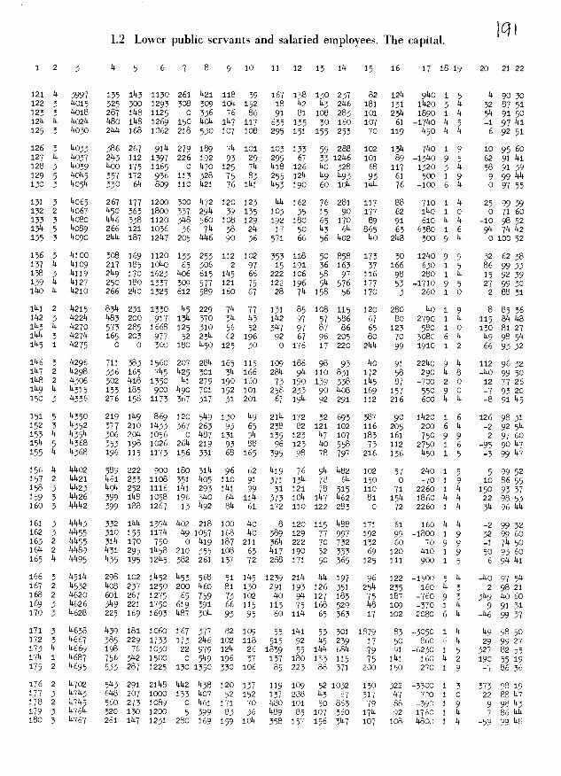
916664-09801LoIL% 9411111 98Lt1IoL169L1094LoI496661064-996L49806L981?01ooLL61%LI4961 964L44ico%Ç-8040411401 ?4

9499L-6iOL?08100?1L4996i 44061190911914L4114%T

44 ?9 L%4T0419-166L999991L? 666?Ii909904LI6%?4

0496 611o4o4-496L9110%44

L4 6699-99090?lOILI4944914 166iioL4-601996z499109 Oh6ti446096-L9I4L491LzT1196?4909144?94?1449114 L6 o-4oo4i-11196L6I1111

19694T00611141149%0409 46046101901169444ic04 9L1-66OL09141?4LOL09 6614610091-66161L66LL14 661-11909119ILl9994ii

99 96ti9109??iL049?ill 4461?11i099194119199L9IL4 460419109??iL0114148L44 98016TOL-0041999L14 6644109?L4lOI18116

L9 664-4To4i94191?L6L8LL0646-91o4L?lIT4L944o11

09 L6166o4L191491LoIL

i4 ?6z-11900?40?911lOIIlT14 86911910111106L446914

4169-111100991?iII16??60146L-06044L41691909069? LL?T0iOOL-L949194464104 66oi-81106?84?LT14901114 96?1T6090?16094686

?44699?T01616699?0??LI949669119o90OL0940196

I0944114999L9Io6L?09L9994L4

T0909?0?T4ii801

T09?40LT944T60ILI-44LL9L4i4109?96911L6941049991L44919460911044LI94904

600499?0919994T0949494999941901916690LI491091?9LLT0641IOIL98LIT18?9L

9001-9L99190109I004194646ti64O?4ILIT999?40960941-69TOI9911 441090941lOI99?64

11o4611OL44?44110901-19LOT09104T0691u-14?TOT49?90140i1I141191911?41T o690119L4?041

69108?14116644ooi199o6901Lo441000941i1911991?

0441 o4T418064 000416L6?Z040199?4LI44L1LL4L910901

9044691164619046164L494611099001 04119944ti1491

19?194491144%01?94916190o4LL4oI6ti9L1191?1099641

16941L9?Ioti%961940146?19191114o1448011t194081006

1449414L1161?99?9101L80940149?L94449164 011699

LI4L948111bL 069 0066L?190441b04111411L

1i8?Lo?0941

o41108100494114LL60144119991oL41141L166??40441

6941194141LL4604L4%I419909819190449090144?44i0111

9994ozL90I9L9494010949940?IT96?L4%00911L11004OO?I

I?90116099?4411946oLti04911?6I9??L6416916L?916

04491?1901909041691194404?IT6049044611I?91910411

91LI91419141lIII0169L9

L9119?L9L114091041O?4119L1146L14L?0944LLo?9994L4LL16?8t4æLtz961

L9?4444699?4L1?liÇ94LL999I9L196961699994LT680494L999Ç?LI1816484994ILT

69148081994oLI1?? 6%9199469169?1090199i991L4?909?449zL9IlOT96?91494991

461 4i46t49146?1496891ii9910LI9144499?49144101444i4191991144Çt1+1t14191

8816641991409199166491994641?4?11094z*Ç94144?199119111L411??69410999941

4ii9619949t441961444994941i4190?904441144101?LL4144941416i 61?o444141

9419L?9449404148144T4149116919191049049181114919449619iL1T494IlL96?94991

004Li141114014919L?9Çt1t1T49?414oL?9949000?60i11111419114?9494I?9?191

09?99?01199091091o4iL1T91164iOLT611?611114941491LI?60199L4169190400194941

L9199?o6oti4481T?I99?69011494184499909094441494 o41L909??4TLLIL9149094141

990444o4041?LTL444tioti46114LI00964o4901?II49?L4oh*L?IL9?99444o49?I

99199?0499441191110911910111111118111L9?9TOlj40044z4410941114111441L664uT?I

4u4?T

L41944t1016414699%48101099OLILT980L4Tz4I4

601611L4i080

4??49901044091L41L%9614464919?t1

16414911lOI111446ci18

11110946464Lcil41199609lOI4L

46116?o4i1991?641149114

ILl99??LL41061L149801li?99411?L9I61169409991011909001

OIT1LI199990141%91199IiIT4661914iTL416011

9L6191996

864644918941196994641144196T411894?4946?LI91?611041

961L910?1%44?94?1011410614L09106111699?9919%

991601411491

9L10044?TL91696119L6L11c1494L61111419449141LLL

909?L90919618014LIll901???9949116141L6?911444lOT111

99IL49406o4LI9?94091?616119014440144i64191998110?I

0614i1919L

144?494L9119199L811L946?6?46441401TOI1L

14146?901LoT441449LITLuI1816989L1991141901941L9T64811

L? 1904199994I94 499

14991

011

6

004 66L?4

64 ?64111

4466 994

84 19146

14 i 0?lj i1L6914 9601-11

09 ILOO

64664?9

44 L609ii 666664 1694919 16?94

09 46016

14 1611

19 L61-404 16tiu

14 L14904 0694

1? T?0?61

WIpwdi(ojdut pis puiiTUuiAJS qqnd ioj g

1ujidtzqj(o1diu p!JIs pui jUtAJS zqqnd JMO'JL)

çç 96ço99?6ÇL? 166T64099916699644919?c?Pj4644ot931940T6104931493?1108hd34dTL6ÇLt1o4o4LI49c11c4164436d?811 9L9L6T09cc-L99cçoçL6991OTT40?9Ç16dh04?81191096oo6?L4439d?9Ç 08o6L11ToLo?11939L?6L91ç369Ç908T09981Ç43119T9ç11ct1ccçLcç11 4990T00?-ccTLTT39011*tl}1OT0446 4 06916111L9ç01443

961çIo9iT?TL99dol1646TT4L?IIT09? 03?9O99t3044334 1199ÇIj00?T?lj96TIt4L6oeo9L1119i9Ç119Ço11LlToctp419tT4Zt13tc 66Çi-cIloc9Tçç?IÇ03104341cL11L111911144hioo099TL9119909143cc91 963ÇI060T-913616LT64T961?TTÇ69413011 OLI010?oçç1L11L91143

9? 964106119T?46909I40T4011LL9640119911ç011Tc61ÇÇ4Ç41j43Tc?

9c66 o6Tc0611811Tot496Dol094LLI931946c00400011114T

T4Lc9TocTI-96cc0LT04091oC06OL00060011?9c100901114T633811 LL11911T011L11LOT93T91ff1L996T43?1jI3619c94T399011113690L64Ç933

9611çoooe61119166oTIL466ILc9c96110941c3?o3L09cc3L3Tc 9661-IIT0891968ccT9L6ç9ç999499ç193c9oT dc 316cccç

cc 96341119o4c949cc 9661L9?L9c49ccc4LÇo4TI19çc969ccç3d 961p111101469OLçc1194IcIL9co6T0LT6311LT?ççclLdl31?1111ccç11?303 369T3dIooIoLI9LTLçdL911?T00999tOT9LTT43441LL36L99ççc03 964çT091146T31TdL913893101199LT1L0361I?dLo430d4333?114 11691110ç11çÇT3693139LTOT1149664911c9L9?cczTLLI06116934çT??

011 66c1110096939c1ccc66ThIç111910400Ç603cc9I34?6tç893cç03311cc6?-160043409L04TT0o6ço?I4LL00?0o?10901190934161?09 9696T909dc9104943 9963T006?OIT9930601 000911?19131? 001 11T39O3TO11TIL?461?cT6311ocdL9T38LhI04969LçTzTLz3cTLTZcd 969110TOLcli401L6I?c4Lh138?11doLocL891ç9c999LT?4391?

9d 966911109111631119oddT T4L?T30?Lcl40190cOÇT9I69T1TO119614dcl?h 001 113111096TOT119LL?69986TT99oLIL9cL11c00311193h3cc9Tcç111?

09 d6T41ç11o11cT-d6çç3986119LTT916T901439LTL039190d?9dOLTc3cTz6L604?90044010406001L60911001Oc?04096911?0699TT4T3T?611 8611611ToTTc6T1d?1cçL9d6L1611699L10611cITd9lT36199d9014cIT?

9ç 661t13011T119C9Td?11941111T9c461119c63?c111Zc?C?11160cd01?L? 969ç60301691L11?9c911011Tdl0116iL?01?44LIco39Lc990436036i 66T-111oec031601464L1891LIP1T81oc9ccc?ç93Tcd?9690904d803c3 66OL?dT08-IT?ITt9144T?TtrillidL3913?0113OOZTT3L319LL043Lo?LT6Ic03o3c99TLc111111LdIL?T091119111ccoc11g?OcOTT91106116904c90?

6c6?1110ç1199oc?LIZoIT960114L96d?L99 ooT 4cc9390cç4o61 99?TIçiOIL9L39L44?03?L9T39LLco?ocT0691i6c696çi1oc31103694L?-4T0901OCT30c6Ld?cL9139c46coIc90T639c10913cC0110c11co?31 369O11o9cI?I1OTTccçoc9cT?I99OT9tjoT14609?1L119?Oc330?911 OLij-I?oI0L91O?T333111L9411Lc??3?66L3?1499Doc oo1c?o43To?

1196991o*r64c?0?do11?T?114dT9T1Och oc?03919?d?96Ioc300?311 39 dd9od6d-30?84c?LI?6c90? oLz9?T09?9T0011ccLItic?O11d1661136616? 6601960193ThI6116c09?LTdT6t1101I?3L39O190364?c96t1Ç96TI9603c-ço6t-991çT69 949oTc63I3O1IcTc3o1IO1zL610116113L6Tcc 66Ç66o6L49LI99?c9T9c1I1T16963LL?cLZILZ?9611oÇ6t?961

o?9c?T6OL???10?1O?c0691198ÇLdI0T1100TL94O?6T4T61I?669119o6ti09TdcÇLIL9L1O9916d16L9LO?L94TdjO6Ç116T

cLtz?oIoc9T499c9?ITt16Ç66IÇ?9109c?1Id9c69c99911Çc6TÇ4 99 PIç11OTL311810?L9949c310199L6Ic0401?LT9Li13?616t1 Ç9Ç1111old4dT6?d1L9?IId11LLIÇÇItjI1Ç11oOILtÇ09hLc911çI6T

099Ic?61ocT6-31110cc019cO?L9?999?T??L13 ?OT L16c90L6?L6ti9t061111 661ç1109TIT??c?99001L6LT311t1LÇc10691coi01146t116914 06o603ct1oI6LL939LtjT9cc9119664 99ZT6T?LÇ11ÇtjÇ991ti1 66ÇÇcTo9L3-116Li696LcOTccl493016?Tc9c90901O9TLIc6tL9T

11 6601c60119601191169?çcltTliIT9160T11ccL61L0T361L9119?91111991

6h969111110t9?1101t1T9?99991646LiT494L6T?IhdI11?11Çd919tj ?69c?11TOÇdI-991od339T?1961 ozc6L919163ccL?ITTLI666Tc1191911 OO11T?1100014LOOT96czT?dcc?O1?T99ooe0??t1094oTc919d 66?11cToÇ?9dT94?ÇTOT1TTI179611Lf90631cIT9966Li?9T09 ?6L?6To?909LocLcI o?66?T9LdL9d1c130011L8L11ç191

? 1?0361 91LI9Tci1I31IIOT69L9dt1Ç3T

oT Ç6zzcToo6T96?T11T11?T611TÇÇT?T?LL911T09T tt1Ç6LT099zooÇÇ 6611T0?T1?T0911z???91T016oÇÇL9ÇT99OT 00T6o110?TT999?66?

6? 969-116o6L-?IT?IT11TTÇÇ?TT0911169690TTL11oL9b'T09??691Ç9Ç96?0961ÇT0999?T?T?99?0TÇ91ÇÇ6oT01111io6?T Ço6Tz0t?9zL6zT9 Ç9LTT0110?1T 0T9L?9Ç0911TÇtÇ?T99ÇÇ?990?99? 09990Ç9z96?

o666?tTO9OT-990?T91?T ÇÇTTO?6999TÇ11T8TL9119ÇTL6TO9Ç9t19

09660?TOITTLz0111? 90909O1ÇÇ11Ç11TÇ9LOO9OOO6Lt19T116?z66o?T011L9T00?1?6T119966TÇ9?LÇ99O911?OO9119T6? 911969TTÇ109699TZOT9?9L19T99?O1TT0111ÇL99LLÇz11izo1i099tl19??6?LI 9L91ÇTo6TiTtTo6916Ç69T 99Ç9911?TT9119?T???T19?OTÇTt9zT6?

TÇ 66T-çTo6Ç?LÇ9T?996011L9?LT06OTTÇ116?9ÇO0T6Lz 6?96Ç9?06?tÇT6ÇÇ11To?oÇ-?ITT69Ç1L9T811199TTIT?ÇL9T11L9?111000169?9Ç6Ç6Ç9Ç69?

1160?TOT6ozoL9Ç991TÇI1TLLT9L?T?ITTÇ0T91900991Ç9T98?1169?T011?99T6L9L6 09zÇ611011T6t1? Ç6OT?fÇL0Ç9TL9?L6TiTÇ9ooLÇ-ÇÇ??9I?TÇT 06Ç0Ç Ç9ÇÇOLT099L? L?1 LLTL9ÇÇ6?9Z99?

? L96T11TT0T9118ÇTT?O?9119T6Ç996zO?11Ç11ÇOT 9L16zT6?9Ç9?IT?OL??11T08ÇLTLTÇ9?LLOITTL96IT9T?OTÇTÇ6???90?01?i10Ç9L?9Ç119?

001 0?ToLLz09T91T1190T9??Ç6zÇ611OO?9?011oo99?9TÇ9?t66??10111911?11ÇÇT?Ç9Ç011

111OTTT198ÇT OOL000T9ÇOÇ??9T?9?TÇ 660?T01196ÇÇ91OT11Ç??9991T?69tlT OOT6919TÇÇ??9T19?

Ç?OOT OzTO96TÇ9TÇÇÇoT11T?9ÇOTTTOT9?991119Çt1?9OÇ9Ç9ÇO?9T09?911 6611T011911To?T?T9ÇTÇÇ916L111Ç1099ÇÇOT 99111?TLo9Ço?9T6Lz611 Ç91166011?Ç9T6TOLÇ991? 6L??T?11110T OO?91?T?9Ç?O?9?9L??11 96LzTO9-611T9L10619TÇ??60T9?9OT9oL9000?69110116116T9TLLz116o1Ç9OÇOT911?991T919T6z?L911OTT?96L9LIO11?T6??Ç9Ç9LT9z9L?

119611?T09?Ç11?Çi1ÇtTLT?Ç?6OTO9T9LT?c?Ot1O?LT9ÇÇ9L6ÇLI9ILzÇ11 66T?6oÇto?T96ÇÇÇ9?I?9ÇTTOLO9T9ÇLo9Ç 96L?91100699T9T11L?09 960?101661ozÇzÇ96TL?jÇÇ?OT66T?LL11TÇO0T 6096O9T9TL?966?T?T0T6-LzoooL11061OL?09L99Ç0919T11Ç9ÇOLLTÇ9Ç6L??T9I?L?11Ç99Ç110Ç9?ÇL9L?O9ÇLLT06L11T11ÇLOT o6?611Lc?TLTOL11119?IL?

zÇ 661-ToÇ?L9LÇÇITÇII9610Ç119LTt111TLÇ009 06TLo? ??10T9?OL?ÇÇ 96??116O91?T11LT?Ç9ÇL9TÇ9OT?TTOÇT6?6L11?O??TLzTT6909Ç69?9? z611?61oc?ÇzzTTO9TT 6?Ç11?L9TÇLz6Ç9Ç?LT9TÇÇo9Ç?O9z99?ÇÇ 960?909??TO11LT 116?9Ç?TÇ699L?L9zT Ç9?0000009TL9zL? ?9?iillÇTO?TL6Ç11TL??Ç91Ç9TTO?L9L9L11O?11?09?08Ç?66?99?

91 ?96ÇTOOÇ-96?Li9Ç6611?9T9ÇÇ09ÇL06?o6Ç?ÇOt?O086Ç?Ç9

911 1166Ç61OT9??11OL6ÇÇ?6?TT9?T?ILTT1f9Ç?006LÇ9?OT?119?Ç? 66L?660?To?09ÇÇÇ116L?60?999L1Ç6900111?T??9?9ÇÇÇzÇ9?11Ç Ç89Ç11110999-6199ÇÇL9ÇoÇ6900?9019ÇÇ9oz 66T011???fLo6Ç?9?ÇÇ 096o6O9T96L9911?60T991OTL99TT 99LL6Ç?Ç6fjÇ969Ç?T9?

o? 6LÇ9ÇTotÇÇÇzLT19LÇ96?T 1TOT?T119o?O6T OL?ÇÇ9L9Çz09?Ç? 666ÇT0cITÇÇÇÇ99??? 6T??T?9T IÇLLt119LTÇ? oz?L9Ç? 6z Ç6-t0?T69OOTz9Çtt9LILÇ910910ÇÇ oLT 091atrgÇÇ9ÇT96T 96L9ÇT0119LiTjÇÇTTT80T9ïÇ9TTTt1IÇoOO0T OPT169+9Çz Lz Çz 669-116066LLT6T0111TT 9T?TÇ119t191 9L 9T96Tcz61t1Çz9Ç9Çz

6T 9LoÇiToLLÇo66oL9oz6T6Çotz9? 6o? o8Ç oo6ÇT9ÇzÇÇ

1166tÇ-111oLz?Ç119TT?z6i 9T 9T6L1Ç9T9ITtO0?T89T9096L1Çz

6611?-ÇT069zz99t9L960996ÇILÇOTL9Çi1i1TTÇ11Ç9LÇÇÇ

ÇÇ Ç9oO09TLT??TL11c6T9zÇÇTT61oLT9f1?6LL69LÇ???Ç11 OCT091iT6oTzt19991L6LIT9T1109LÇ96119T ooT L? 9TtÇLÇc

zÇ 66ÇTTo6990611ÇLT ÇÇT9LTÇ9Ç90OTOÇIT01009ÇLT0?Ç? 96Ç11tI 0%Ç9911e911091L911gzi?919011eLt1 9??zÇz?LÇ6911 969T-ÇToL9116191Ç9L6T99116TILT0996ÇTt11966oL?Ç6LOTTOOT?009O966T9LT?LI?61L90iTÇ 09T11tt6996oLzLiii1 96?ÇToÇ11-08Ti0? 6Tt99L1zÇOTLz116ÇoLt9L?L0LÇ69Ç911?

ÇÇ Ç6zciÇ9o6?-T6Lo?LLTL9I66T119T09T6TTL096ot9OÇÇÇT69?Çj666Çz11o6TtO?9ijÇL611zLÇ9I9ÇÇof1TLT1ÇiLz?119Çi1tj?11? 69ÇToo6LTÇzTT69TOT9??1199TL0T9ÇÇ11?

611L6z-TT001111TTtÇ80900?OT01000TLozL69ÇT11?11Ç 66L-90?OLTÇÇ9Çi1tj6119T 09006660ÇÇOCTI 9?T?9?Tt

zT?0?61 9TLT91ITI0168L9ÇÇzT

1udqj sAojdm p'p pu SU1UAJS i1qnd iato'-j

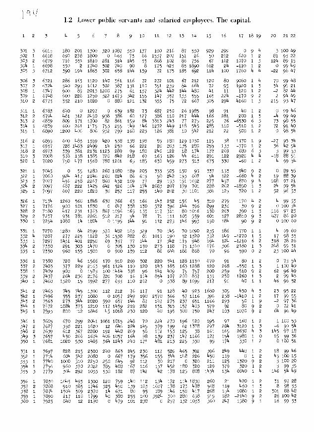
44 669TT6o94TLl096440T ?4164?O94?ToT6610o6T??TOt94?6LT094?t 001 9?6OIIT?-?8T414949O9094 t6Ç 00144?ogÇot166LiOTTLI?o69LT644811 89104?T090TILT99?LIII94191T69T4609TL9iloLc?694IOLTIiL9LT94444 9694T091161T9949Lti4LT961L09140T64To4t4?4911LT496016999LL449? L6T4?TO?tT?09?0491 ITT?LTt161?TTOtIT646O?TOO4T46114t1010496T944

6iti9t1T11T01109114T141T909?T9LTt1?ITL99To.44401tjoÇ6LLL444644 6641 o46L66?1O?09T?41iL4T9TTL9T801149L??O?oL409694LLI0001 66 O?T4?ITTo6 oLT04?TT?6411904? O4?0T4000ToiLL144441 OCT 411Io61TO4t9?2901tll44T9446LTL99O090?t411091TLLT?4Ç911 669T?1011116i964649119?4LTT04?4ti499O+? 004?4T?9?9L69LIT44

14 001 0?IO4tILT460464ÇT?T911LLT01?4iT1194911044OTT99LT04494 6641010961141L?T99T1LiTL4?64T961191L401 9011IIL9T99041L49L46t69T L64111411049?49TT9T944?T44T?L19469?911-tI?6109e?L94?196492?ti6694TO?T4110?26?9L4T ?966T6L%4111I9119?TO?9TT??944L?9L?Li444 OOT T?T09TL646T0?961OL?i??OL9i?4TOT T9OT 110?66?0294092T9t4

611 96119?6OLOTcoiLo4L00646T011O?I 02 9TOT 411918T?T009464LTÇtiÇ

Ti ?Lo?609?66L4°tiL4T414T41?9?6T?6411T LTIOT?T4L41180T?LLLTiiÇ94 26?-6To446?99TTT49L4?4L?kiilL9tililL49064O?o?ii4L?4942?ÇtiÇ44 66Li?TOTIT-9429649TTT L4994oL4?o6T611?L4OT 00901LÇ44496+LT?1

464?4t0411404089T4?6oti9?TT6LIT9L?T??TT004T41L4iL491L?1114

?4 96911TT0196LT?6691 699440?9?OTT449LL?66T41O?4IO91LTOIIÇ

i 66?41O9?1OL?44TL4900?LOT4919T9T90Lo?L9LT?94?119?L4tiL?6446ti 96?9?60TL64?00?L4LLL601TiT969L4IT1T OOTLLLI00066oiL19446i 001 TÇ1044-99?O?T99?I 491491Ç11T0?TOTT11?TT T9649T?6LL4ÇotiL?L44

iLLo?T08T6oL9OLIT 9?IPIo???o469?0T6oLI994T91O?L094LT944

1111001 4??006496OL999991 t9 99?TI64T0060OOLTLLT096oL4LT446T4 6691?4T09T?9069L9094T LL9TT4L?041o6T4040OL1T404T6?o44L?9? 96914?9OT?T-1?T16T906LTI?tiÇLThiTLLL446904??TOtITÇITL6?LTccc44 96LILTOL?I-61T?44O?4T ?40614T0TT9?9?944T 949?TT4LLL9?Lt1?ÇÇ096611TT0LL99T44?060T OLL11TOL6?Çoi?91oL466T?11909?IOL?LTT44

09 001 0?6061191OLT466911TLL??TTT6h1iTL6TT 011081iT0801114?LT0440? 99L9046019?L?I1096444OTITTTL9LiLT??TLT9??T9LT46L4?L?6?44? L69IT4I06449?04T910108TT4LTT44T49T960T L9949LI14?LT1091L?9?ciOOT O?6oc94?669964liT964?L4o4T944LtOOÇ9TTOT0069LTLTL?444 66?t10LI66?014i941?L?Ç1T9914999L049819109409?TII4TLT9?4

44 96?4?TO?L4?T994TOTT 04?O?011144?LITL4?04O?9TO??Lo9L60LTL?4ti6611?4ToL9T-?9?9??bL 6LiLo?499?iLT19T9?4?194?II???L99L60L?I?cI? L690T116oL9LLiLL??LOT TLT44T6?LL601?411099L9??94?911LL0L464 9961?11099-??TtiLo946T?1?044T999t1?909?91T?LT1ti?6O9OLT??444 6o?6oti644TL444604T404ÇÇ440?69T080T 09?09?I44o4IOLTT?c

ti66I?T09-0444L94T44L?64i04949T49IO?T O9LO94TLLio4Lo?oLTO?4T4 9991-11IO?6???IT6?TI9tl9?T49T6981??190?L494T94T864900246T64 6644909969?9LTiLl81??T01?O9T6669?4?TT TT? T946444L69?914i?194?I0LL-44T44?08?44T4oO????9964?iT6611?c90T 9?LL469TLT4

i46L?-6TOLTT94LTTO4OT 6?TO9T49861941944O?i64419i0094699?9T4

tÇ 960?Too??T??114OT194 9T09T662909901 0OT0689TT4

011 T6LTOTL-OTT494t4TT6ti1L?T9IT611T44?44L4LITT9?0096499T11T4

ÇL 96L4904499L4?4LLL4t414418641T99?9OOLTTLT6086489?T46ti 66i-4TO0T8?99T11ttLT?OTT98L?I09994946041?I4T1t1629911660?T011169649619?04?L99L649oL6?TO01948L9TITÇ

Li1 464T?4TO9Ttit16?L99?L4L444?TT?T098 00?OTOT?44)19?0146ti 16?60LT-1?9T4L44cTL44L11T441tiÇ4L91 ??40?T9??0068129T604

?9??T 0TTTT110911 tTt1?L41T9LL?OO?TTO?49oo6L11L9T804T66tc4To?6T46L19911964?ILOITT4TL9?04T9T46?01411?L9Lo4

66OL11T090690T?TL9101?L??L9TTT94OIITO?TT49T99T?L949oÇ

Lti 96??,t09L1OoTtTT?6948TcLT?L641 tT 9L9499T1161064?TL94o4611660?T01111??990691 494?lLLTg06otiL?040IILT?0449699TtoÇLI 6gti?T4TOLOT?9TL994L98?0T994441T1114T9?OT9T6L9TL6L99?404?? 46T9?IO9?9?049?TLTLO?L44T99L4911000918L?0699T99I?06iiooÇt6o66?6?6044Lg9T?OOTL41o4cL90T o4 O0T TO09TI994104

? T?0?6T 9ELE914TII41?TITOT69L944?T

Ifl!duqjjz(1di PJ!JIUS puuujqnd JaoJ

piidiq1ojdm p.Itjs putt S1UAJS MjqndMo'J gI

t4 6691i094991011049941L4998t1-t14911OT 01009144i1o4L06461olti09lI11o6îT4iLtjT4LL 1TT999449lotIi9094161019T9146î6Tt104 96611OTL091001049 Oî 0040OLo4aoL001 00914TL09010146î9îtt1i1 t66011609018164L9161 iiI19199091T10046oL49t10ThL4ohL96i6TLit11 OUT 9hÇ1004o4i9iit1149091191L948061014099OUT19h6L449t16h9Tt1

ot 96t1b1001-L9î1119119T tiÇi0014401441811T901 oæi 41LT9Çti9191L16T4ittjÇ 96i9hTalL-091041bLOT oÇr6LÇTIbOT9L19444Li009T914*1401oUtI61111181 16ÇITh9009-9110bL9LT U41 c4 4LibITThI6901 019 OOtb49Loa4î19161Çit1111 96911-b60*181-69L94664I ilT9999401IlT994099000111401 9T941T1611111111 66LI9i09019614LTL941 LL4or416hoIlOIl9hhT 1949T01499o4Ltiol6bTTq

99 1901b6090191140196906091T4T1L4i0911464004T9111194646101t*14 6910411049146014I1TI 06LOTL0909141*1179469999110091014616otiI 664111019OUT4919411 44TTbh0h09176690T1 00409616h940Tæ96T9017

44 66016ooL1T9661 099 OL91LLT16191T06169Lt1t19419649916TLoIOb 1619hbT006L440441141 091104L9Tbl99149109OtlTLL19h4199161901

14 001 4i4T04118L611941 041911194LI4Ç*Ib4611 1111100419091*141916b4014h 961719T0161994LtzTIL9TTL14174L441ILTLTOT 09901014919941416b101714 46T919T09b411i1t4T9L911TTIl499OIl49T99LLo604610191111191161901Li 96T44T09019t1TL4176T9961L61014IlT949ÇIIT TIl11619194001o4b6bbolOb 611464T09646914LT1941TTIlT19469T6699qLb9191i40991116b101

bI 99Ot46ab4l-194bT9ll961T 118104191061916946ob041141191114T6b001t1l1 669bI091ILTI4L194OObILT411996616I9T 09L9bbt14L0*1494161664Li 644L949099T-9909444bT999TT14ÇtÇ94914T 09L9611LLbtiti6i16b969T4 001 oIi09141oLo401609TIT004140161769I9LLT0h09L9116TL6491 1614bîOÇLi-LT1L644b9ObTI4410b9b610919L01 0o4bb94b0999016T964

1 964bT091TOT199141911861191L4h6Lb1T999094T449194T4906T469T4 6649bT04119110416001 4Th1411494*111419ITT OLI9T14h6196906T164Ol 16 o4b9o8941199b6L9149LTÇTtITTOI111999'i9941L14t19t1t106h46444 9616b104919h4919oLL4b 094ITL09144T4ToI ObL00Th96191916691164Lti664111016L491199Lb9T4L1L4bL4TtITI9410410414691t1O41968T164

04 001 0T9019-991094oL6094910041091OTOT 0091 4b4441O9L0199To6444 9619T9T041bL9491941T L4TL1b44TL6b41T999Lt49IbLil OTI4099b69444 6609bT0414919Ib94T 14T9L1TOtI9Lb44199L4994bLT0100119LL9199444 664ZT06914LI06464b41o4b90191144TL9oî 00161LTZ01994L9IL8991 96oz6 09499449b94101h44b64TT499060640199691LLi6LOTO1L8T994

94 001 9TTI O9T19h9491 oU9h9b1OT6lOb90699946bTO009b499T994at1 696T-bI0111144494149T1 199444991b6b611Ol004149104116191*19401 1696bTO9LT9T4OTI1041 1901hT6L6699TLb4oO4TT°ti0ti49919T49494 96OUTbT090194140990990bL4bhTLTT1L19ITT 891001119h 0194919119491 4L694140414ILTT149T0641T909417499T0140961L8LT96Lo19bT94

9T L44114ToL6L99106OIlILbol919bT0449101o69T0L170449949b09409 4690TbIOLLCo?*711401*7L9904oIT4LTOObLLTI 44o44T409416149I6L404 *16L-9T041091LO6TLII96191919TOT64161068Oq9bITb4996149b9L491 OOT 61bI044T41196116T99hL114LlITLLTLLo4179T0IT1OT40491LL409 6644I6 o6LTIT919Ob9T OCT4LT494L194T914T 4149941*1619094Ub949L4

o9bLbblOT099194Obb4b404h019T?b49OUtilLb416199b9T4L4I964141o49bIb4LOb9460441104990T4oTL4L1T940T19410*1114419b17L9a4 176Ib4a4LI170T9149601 4LI1*117TThbh6TT449*7114blOb6Th109T419b4L46T 0914T011LI014oL9041441L61L919119bU1444LLT90*7641T1918b1L490 0019Tb1041-ILT001OLOUT19404900141106900?9b 004b4TT1h19T1L4

L1 9691T1009alT9IL911101911114TThIL9TL891L9bb4l69006ObT9ToL444 66949io4ÇTlIT4L09Th 4h61444L6b06h4t14I o*IÇ9TL4z0044609b69409 160bI0914419oLb4ob909094zT4LjL990017a4bT0499U60909199404 19oTTOtoL9449TTT9b4911619L16T4TT644blI044401740116409bL94L4 9649Tb600418Tb90417941 T414917441bL9*7149900011Tbo4to9T994

Çi1 464ÇI06?ÇT1L946gi9b196ÇLOT 4T 6166Ç9996ii1 Ç911L4o9b49Ç44 66I4TOijtb4LitTÇ49LT 491j11T98T49T9bbLioT 8T404hbL44T009bt19bl 66T-T0944604bbob01164TIlliT*191T9L9tT9199L91TIb40t11L6Ub994t14 T9891b9Oi1bTbZ91?64ObTTbb9ÇoLT91TIbb004 OILT069a9ITgi6LTb9l001-b4099-00109?4660069?09*1oo4b6T 099008To09Lb6L199

bl TlOl6TtLI9T4T1T411TTIOT6L94179bT

4Loo4ot46t4iL6Ç9o011 4464oL6i0444Lo44L404 o4i30I1909f119f1?2 09104 49921ooLLLiLLf1904 f191

L492ioLOtjI2129L44 49104 661Ç90TL264499e449091i4L2ii0441406402f1941oL 19Ç6044490240912L29f1Ç 4Lil-210461-64oi4i4of141 09

92 990Til091024bLf1ILI 9L1444641-TioL26449tj0911 Lf149f1 66f1121092201f19214T f16109 L6426ooe0L20241992 09104 f194ioL4612ooe699211

6604Tof1L1941494949412f1 iL4144ioL4219429f1L4912119642il024364294004i4 669T2T09110109196L1 9414f1 46ILl210111420926991 414

0f1 L691121

09 L66L2604 001 121

66L21

44 666f122

4f1001 62T

09 96219Lf1 66L2644 L6OT2f1

9f1 6632TT

2f1 001 L22T

LI 6L6044104 96 9T-T104 669LTf1

f14 664TI

09 462121Lf1 99142f1

6f1 964f1T41

Tf1 66941T

92 49LoI61

0f1 964iLf1 664oT206t 66L946166oÇ-21Lf1 T9091T

9903i1

92986421s4 001 02f1

44 9621o4 Ç62I11

22 120261 91

I'T!d'JqjsojdmJEUS pui S1UUA1Si1qndi

9944t491401Lt94119L0Tf11494L9ÇT691jL164i904694 L44 oi Lt1t19L96lo99f1214f1L,rLf14Lf1241 o4oo41o2t141i Lt099Lf1Tf161402L6L1 09L41i144OLL420f1iI99f1

442oL1112912222 o944e9i44t14144641T49f1L63409443t1129919L46614111126L1019411191149149004T4240111 4690694t144002149441149t114440444141j1L911 0041491æt1L49904412Oof16942091L9944f1940042 9T æL14Lo41119f1

6z46926919429913 O4T 00214t14oo609921T09f14412848f148f1492111 oot4449641f14421iT2 90169269244410109f12944921o621T94111f129461940644600690420440491141211L4f1669110144290124L04f1Lf1If11f11299L61TT94f1

6o4992141212294f11 4L00f1299f1f14119L91TI44L6r411L4Of1TL6L0294t124Lf1041114911f14f14429224L1412LIT4o4L9144449111144f141449L9614916Lf11 o00064114111z46of14Lf1oil0424f161 120491L4496614TTT14f1

2Tf144f1f1669221 941919199f1ILL190111o4f104206T9011f111902 42461929001iLLolT61ftl444i0649419tjO00112 622 6l4of1LoT19tf169444219618812911 09f1026191402114f1401T

L92004f1TIiL1144f11949T06444119440119f1f1

2424444f11496299TL004290f10L92040114trtî662009420261T T9L09426910201964011lrtlll644LL44tc6490614641966f1144201T4t1i1

9LT0091494f11Tf19601004196f149696101T2tt11

262049211036921 00f18242 441029991011Tf1f1

L4tjo002OITTOOT o4Loo00414910110f1f1911001L9f1f12TL02f16f16r211112011L41o1i6Çt0610416046616942222103491004194101194f19221f1194f140429f1TT 4L94t4911141Li001011L4f193421L942f1194919Ç4923f16202L49001194f1

94449919414429001 1160341lf1811666144t49f142904442Lo61 002094Tf1f1f19921f1966111411

4L44912146164rT Lil4f1f110644L419266244f14010914124499ooLL64224142L2oL96I24f192404f1ttj161loTi 62f140f1l24226f1Lf196414f1

9614021f1LTL6L22T 09400f12Lf14096ti61o4f1992212222619961 291Of1fll44f191019496162102 244861Of1T9*I1 19100414oIOT9c9629f102202918809196LÇ94f1222691'4i169L6TLit1

2I002f1Ç349T014044f142244L9LL6I92t

O29190Çf1L2t41T 4001 009126LiLd6zL6T4iiÇ4194429t1914L601OIrtI1020231f1iL6Tf12f1

T03696119L214Ç900902140f1l0921O96TÇ2t1L149901 11 96190f11 Ç14 &L191f1901096I2f1

LOT2290TLII4620O2 4090146461Tfl

TII0169L94iT

042041022241 9f1ToLIL12oT4404291004f191104492f1OT

099l464L20I 09f1oLoi261L624992 621

0f12121f1444201 042002120f1404L641 4410461L91604L6f1l 4f1TOLT2L614621o61120L4T9f12Of1L0041 OL

0040414294291 044oIo4042692994L902-9L204426091 9L20294-004404oiLo6iOLIf19494f126L061

oLl4L126444ci 242000194102224f1f13T

006f164144T4f19190122T29L226f11 4010444L3I4041041 L12

021-411f1926911 091042-L42LLf109L1 911f1olLi6Ti2T 6ooL269100440409424L1f16L991 2L4

0f1T4Tof14L69Of11

0If124214L20094

0126910406010L44211L2LL 02106111tÇI0914910

Li9141t141

1.3 Skilled workers. The capital.

1 2 3 4 5 6 7 8 9 10 11 12 13 114 15 16 17 18 19 20 21 22

1 6 20214 194 120 732 356 1344 344 58 51 69 38 16 53 78 200 1 0 3 89 23 2 II 2081 223 126 780 41 132 45 33 2914 68 73 105 28 125 160 14 5 -19 96 53 3 5 21214 131 96 8142 105 210 141 82 944 65 35 113 21 157 260 1 6 0 96 148 14 9 2152 1614 91 693 69 111 52 314 168 141 23 331 137 58 0 1 0 -21 6330 5 5 2168 132 136 8111 118 116 214 56 117 56 443 35 944 152 530 1 6 3 90 116

652282 203138701101415714852 3011 2538103 35 95 141016 -109352 7 5 2297 196 92 993 1147 1140 514 59 91 55 111 177 145 1142 -120 9 6 114 97140 8 14 2300 332 296 585 250 35 50 59 20 611 32 1414 20 191 530 9 5 3 98 45 9 5 2398 281 135 780 2 125 81 30 145 85 44j 252 2146 1111 -320 1 6 9 90140 10 7 21409 93 118 833 1844 iI44 69 121 195 103 56 237 92 165 14o 1 7 0 95145

11 14 21473 201 122 975 159 323 176 66 88 115 141 944 42 3 2140 1 5 -6 100143 12 5 2526 218 136 783 201 2044 1214 68 78 86 95 122 20 132 350 1 6 0 99 La4

13 5 26014 257 162 986 2044 113 58 67 7 71 36 89 166 106 1680 44 6 -16 99 44 ill II 2606 223 139 1312 6 250 78 87 110 67 7 62 5 186 370 2 5 6 96 32 15 3 2611 250 177 1081 1110 133 87 106 4414 1014 61 61 28 68 130 9 9 1 73 36

16 14 2683 232 152 1207 329 60 83 71 1114 416 53 80 66 1141 -190 14 5 7 814 33 17 44 27044 293 217 935 170 231 119 93 449 118 1143 69 30 126 270 1 5 -3 99 50 18 44 2711 217 1914 982 449 92 447 32 26 86 57 277 65 163 180 1 5 -1 99111 19 II 2756 158 171 712 1714 264 117 128 292 123 51 272 90 157 -770 6 5 19 9839 20 5 2786 2014 115 871 68 3111 14o 67 172 744 52 2146 1142 126 1400 1 6 2 92 143

21 11 2870 205 118 875 70 3144 87 844 265 97 60 351 83 152 -1100 6 5 144 51 14o

22 11 2872 150 126 1300 326 202 78 138 121 117 96 2214 62 0 200 1 5 -2 98147 23 II 2880 252 150 885 137 187 96 49 2148 443 21 97 288 121 230 1 5 9 95146 24 5 2975 389 123 1050 130 118 514 129 26 60 38 138 83 80 290 1 6 5 88 442 25 14 2990 332 156 910 180 107 55 110 270 36 107 2814 100 101 690 1 0 11 98 53

26 14 3006 387 198 870 142 299 122 107 443 121 71 180 167 138 500 1 5 1 98 51 27 44 30446 256 83 11014 260 1744 56 86 39 90 142 126 391 128 750 1 5 20 91139 28 14 3067 2148 1344 11149 144 210 51 86 325 66 142 171 24 109 1630 1 5 17 98 50 29 44 3160 1480 2014 910 196 113 73 79 52 81 59 379 107 183 610 1 5 51 99 I1

30 14 3169 591 165 937 76 109 77 39 2447 73 11 85 72 177 1200 1 5 514 98 14-44

31 5 3197 2514 1142 12714 178 65 90 57 82 29 52 213 259 141 200 1 6 9 8 441 32 14 3209 833 2143 814 Q 253 97 442 170 102 143 158 1014 171 -130 1 5 -96 99 I1

33 14 32145 5145 227 975 225 208 82 30 2140 75 102 80 23 113 2980 6 5 7 98 142 344 44 3252 228 58 1105 107 2814 56 69 1148 80 145 253 320 1147 -750 1 5 82 100 344 35 44 3309 14414 158 11014 1145 159 90 30 93 78 614 97 263 131 900 1 5 19 96 449

36533449 168133991260201147661007155238 82 93220016 5097143 37 14 3365 215 3044 1125 277 1409 76 1147 1146 115 50 180 20 113 14140 1 5 -1 98 53 38 14 3381 381 168 9442 92 136 62 106 302 135 57 295 86 195 6140 1 5 -6 97 1414

39 3 3381 251 125 1805 260 391 62 39 50 239 81 165 2214 120 -3500 6 0 53 91 28 440 5 31412 139 185 1136 379 353 76 56 1144 105 71 226 171 111 4480 1 6 1 99142

141 3 31425 511 330 1527 298 130 50 449 7 39 14 70 85 223 -1150 44 44 158 79 5 442 3 344447 367 262 965 513 283 31 115 1430 449 92 447 36 131 160 44 0 -19 8621 443 44 34479 1114 102 1637 150 14146 132 844 225 511 31 3514 90 85 180 1 5 -11 99 53 444 44 31486 299 131 1076 383 1400 1h14 82 136 115 51 325 185 118 1520 1 5 -7 99 142 145 7 31498 0 93 703 269 4449 80 83 1311 139 78 6148 102 76 1510 9 0 1114 944 144

446 3 3507 335 282 1462 133 2149 78 109 169 78 70 117 441 189 -370 1 44 18 98 148 147 44 3513 181 58 1155 155 589 78 149 7140 59 17 62 8 644 2140 1 5 1 98 51 148 44 3520 313 171 1220 275 298 123 1344 87 105 91 256 544 160 -120 44 5 2 99140 449 44 35142 4434 1844 980 2514 332 101 544 67 70 56 86 919 181 4420 6 5 -28 97 149 50 11 35142 265 153 903 0 319 118 100 844 97 614 328 85 181 15140 1 5 59 98 147

51 3 3605 227 183 953 166 106 96 107 280 153 714 133 32 202 1830 44 14 5 98 53 52 14 3616 1406 271 11142 2147 3141 81 119 190 112 70 376 156 314 14490 1 5 121 98446 53 44 3690 252 193 1201 269 313 81 75 29 96 25 4472 1244 260 4480 1 5 16 99 140 544 5 3733 290 205 869 167 513 113 39 147 90 36 223 123 162 1710 9 6 215 96 344

44 37147 44944 175 14455 4406 217 65 100 55 78 32 209 12 218 300 9 5 173 92 314

56 3 3787 312 172 1693 225 1440 122 62 61 237 65 81 32 159 -190 1 44 7 95 37 57 3 3806 350 273 11400 62 331 101 187 118 91 50 89 121 168 4490 1 44 23 98 52 58 3 3816 1407 261 919 97 520 97 119 126 88 63 573 80 152 200 1 44 1 9925 593 3833 22019013003771414110957 5761110278 85 80 1140114 39950 60 5 3835 180 167 12148 122 593 101 102 86 193 6 3443 1530 166 -51150 1 0 70 92 60

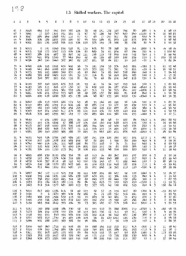
6ti 96 LÇ Ç o cc 113 161 9c1 ÇÇ3 99 991 IcI 936 091 13 ÇL3 9Çt1 3cc 3 031 ii1 6 I t1 t1 oct1 oc3 gÇ cÇL ÇT 611 cLI 96 LtiI ÇÇ9 Lc çc cç ccc ç 611

c 6 LT c 1 0961 913 06 L96 cL 6Tj 99 6 ccti 1 c9lT 903 LÇ9 icc 0 86 11 Ç t1 oiL- Çc3 1c3 t1 col o6L 611 coi tÇ 6gg 3tiLl ooÇ t1oc 9TÇ 3 LIT ot 96 i Ç ooc- Iti L1 3L3 311 1t11 9ti9 6 Ç9 90ti 16 91L1 ût1Ç 09c ooÇc 3 911

99 0 ti 1 06- LoI coT 96 L 6L t19cj ti6 66 98Ç Ç8Ç L90T 933 19ti titi3 Ç cIT ÇÇ ti6 3 6 6 ooL 6Çg 931 LT3T o- 19 oi t1c c93 c ocLi 013 c9ti 113c g tilT

L6 ci o 6 09Ç 3T L99 31ti 9Ç 913 361 931 601 ti9ti 9T 019 TÇ3 ccc 36Ic t1 cIl Ç 66 - 0cc lIc 06 Çlc 19 9Ç1 o6 ccl 99 cc 011 90L1 613 cL1 Ç 311

c 96 gt- ti ogLg- 6T 9903 9t13 L OcT cic 19 36 ti81 3611 393 09L LcIc Ç TIT

cc 66 ti o6Ç 013 tioc tiL L9 ctiI 3Ç L 6 ti61 ccc 61tiI 99Ç ctiti cîc Ç OIT t1i 66 o ti 6 0ti3 9ti3 c3I ?3c L ocl 361 ccl 331 3L8 6oti c9ç1 cÇ 960c Ç 601 03 L6 9 Ç J 003 6cg 16 199 Oti 3L Ç83 oL 96 cLI gcti 99c1 99ti O9oc 3 901 cc 66 0 Ç 9 033 193 9Lc L9c 901 IL tic 991 39 30ti 09Ç OLtiT 9 0 99oc 3 LOI oc c9 6c- t1 ti 0001 08 Lo9 9cl L Lc 39 cIl g 3L titi tiÇÇT 693 L18 Icoc Ç 901

91 99 9c1 Ç 063 Ç3Ç 303 991 c3I LL Ç9 ccl o 19ti LLcI tiIÇ 3T9 ctoc g col cc 66 cl c T ooci- oc3 c6l o9c L c cc ti9 69 dli 091 ÇItiI 981 6T3 ccoc ti tiol cc L9 L o T oo 69g 3d 9thI 39 LLI 6ti3 39 96 39Ç g3 o6cl 6c3 9cc cc6ti c oT 6ti 66 0 ti ti Ot9 ccl TOT ti8 Ç9 col oLti 811 9ÇT ti9ti 911 lÇtil 9ti1 cc go6ti Ç 301

L ti6 31 c 6 Oti91 EOT 36 L9ti 98 163 9ti ITT 66 cc coc 0111 LoT LtiÇ L99ti ti 101

93 86 8Ç g ti o6c- 031 013 c9c 9L 9ti Lo 6 OL 09ti 003 0031 9i 119 1199ti 1 001 cti 66 c- ti T oIL 903 c9T 91ti 611 ÇÇ3 001 69 c91 coti 191 OLd 361 g6g t1L9ti Ç 66 61 86 33 Ç 1 091 9fi11 393 cl L6 ctiI 6l ocT cti 6i 99 31T3 cc 90ti gL9ti 3 96 o 66 cg ti T 039 LT3 cc 90Ç OtiT 9tiT LT3 39 331 3T 9cti tiLÇT 1ti3 LIc 3c9ti c L6

91 o6 c 003 Lo3 093 Lt1Ç 08 tic ccl 99 9L 9cc 9cg 00T3 0Ç3 99g 6gt g 96

6ti g6 TT t1 I 0 03 003 96d 9 ÇÇT 6I 901 9L ctiç ÇL3 OclI 661 11 T9Lti c c6 i 66 0 I 09T d9Ç oog c9 t cil 0T t1I 069 Od OctiT 30ti tc ccLti c 66 9 t1 T 09ti L63 cL t1L 0 911 LLL 68 9g1 83ti 101 TtiOl tlg oi 6tLt c 6 cc 66 9 ti o6t OO 09 6c c 631 09 9 9d3 96 ooc 90T 9l Lo ooLt c 36 Tc L6 9- 1 0131 103 L61 c 6T tid TtiT 8Ç1 L9 69c gTT coT 3l 9ti lÇ9ti 16

1i1 66 t3 1 9 0633- 9ti 909 IL 031 Çtt 6 d3 OL 98Ç c9c odg 061 o9L l9d 1 06 3Ç 66 dil d 1 0091 9 Lcl c cL T iÇ 911 IL Lo cIL 99ti 331 9tÇ cLti 69 Ic 66 3 ti 1 093 991 061 00ti 36 6i 6ti1 c 001 cÇc cog 0001 9cg L93 Çccti c 89 9 66 9L 9 0 9Ç ÇLti 9ti 0I 0tI 9ti1 col LOI LÇ 903T tiLl c6 coc t Lg

oc 89 0ti3 i1 I o6o 68 LOI .d 9 99 L 911 I cc 613 L9ÇI Tc o 6Ç Ç 98

IÇ L6 3 ti Ç 03g- c3 191 oc lIT 931 oT LL ÇT LIT cccl cg 6L tot Ç d9 cc 66 9 t1 i O9j 193 011 ccti 09 tT oo 001 69 tiL3 LIti 09c1 I0 coc c9ct Ç 9 gc 66 9 i I 09Ç 391 g Ç93 IT 6IT jT ti1 ÇtiT 9cg gti Lti91 061 I1 cc c Ç9 9i 66 L- d 0c9 3Çg Ç6 LOI oc LT 93 96 931 96ti 613 6col g Ç9g 6lÇt1 ti 9

Tc c9 0 0 6 091 ti61 99 961 9 9til c 96 Çti 6LT 939 999T cl ti9l Ojgt 9 19

ÇÇ 96 ot1 ti I 0ti63- 6Ç1 OdOl 9g ÇÇi Lti ti91 9cT iÇg 9cc co3T 9Lti 00g t1gi1 Ç 09 66 1 ti T otig 913 19 69g 9 LT c3 39 96 3ti ccc OccT T0 tOj T3 Ç 6L

9Ç 96 01 9 1 0091- L9T It3 9Ç IL ÇÇ L3T tigl Çcc I8c TOcT L9l cLti L9l c 8L 9i1 66 6L d I 0Tt3- 9tiT tilcT L91 ti6 OT gcti 9L L6 OcT oL3 909 cLT cgc ÇTti t1 LL

c 19 c d I ooc 191 cI L6 td 9). 19 Ç IT ccc 9Lti cggl 061 Lo 61Tt1 ti 9L

c6I- tiI0ÇL 6d 9tic 9O99 9 9L 9 19 dcTc63c36 L9c06c 960ti ÇdL 6Ç cc Ç 9 091 9I co o6 9d 19 tilT 001 6Ç 191 ocT 6gt1 39 T 9°ti g tiL cti ti6 L 9 9 o 6ti3 8Tc 093 c 6L Ot13 o 6 I o9Ç 0331 d9I co cLOti cL

L 96 6T ti 9 0 113 IL 19c IL c6T oLc coi 86 99 0T3 ooI 6ti3 Lt 69oti Ç 3L

9 c6 c9 c Ç oL- T3 ti1 t1Lc cc 6T 131 6L 96 g6ti 9cti 3911 c61 O9 9oti ti IL

tic c ti I OL- c9T OT LIg ti9 99 133 LcT 39 LI1Ç Loc OttiT 061 otÇ tÇo OL

91 9L 6c3 c T oLl 613 9ÇÇ 0cc 99 63T Ç9 39 6tt 6titl LL OocT 603 T6t oÇoti g 69 6ti 66 g c I o6 0T 606 6T1 9I TT 36 L6 9c L96 9cc ti8Ç 030ti ti 89 ti 001 T c ti oTc 6ti1 09 6og 19 9L 69ti 09 tiÇT ti09 cI LooT dLT d cTo L9 tic 86 ti ti T 0031 It1T gÇ 96c 9L 09 0ti 601 1g gg 9Ç3 oticl T91 O cloti Ç 99

gç 66 6 ii il o 9Ç c 99 gL c1 061 OI 6Q ti6Ç 9col 6l 0g 00j 8ti 96 9 c ti oo cLg g ccg 19 t?9T 66 c L6 061 cc ccT 69T oÇ t196c 9Ç 66 ç ti ti 0cc 901 gg Lo LcI LL Ç9 Ld Ld 611 Lc 9991 6g c9g 196c c 13 g6 91 t1 9 o1I- 0ti3 03ti Ot1L 3ti 631 Lti Lti IL 131 IcI I6T o LT Iti6c d 96 9 ti I 09g 09 9ti1 091 301 IcI g6 9L ti3I Lgc od3 dti6 9ti9 gI6Ç Ç 19

T og 61 91 LT 9T cl tiT Ç T TI 01 6 g L 9 ti c I

jujrdu SJJ)pOM PIIPIS SI

pTLdtqjJ4)fJOM P1IP1ST

tÇ 6Lo9 OT6i499LT ?6?LIT9LL00?L99t1OT 9011TITI4400419969T091LI 694111?I009-404??TO? 4?I09119011969oc?9691 o4 4LLI0969T6Li?4 66II?-4T0099499??1TIL461441ti1409140?LIL641 0? 9L4t141T1999?9LT94 6601-TT09991006LILT 611ot49061961TOT966494600? 009oÇL9iLLT64 L641T0691IL?9111?09099010?914?4?46419?999OT?L9I9L1

0966614109???94994966601911Lo909?OIL194L9091?L9?969TIL9?4L194 9604406?406Lo41949?TL6T96?0969O4?1 04??914i449?949?9LT99464-T1048-1964114941 09??19LL?09T?IoLTO?L4T496469410969T4LI04 66441049?661L69091LO?LLTL99691491469I?019199??499049?LTLI 96999T014669?L4L9?Li68L44996969?9L46LL9T941?46L?94ILT

9996 994T0911-??94L?9L94699L?09?T411611446?144L6i404499oÇ?9?OLT44 4664049164?491T4L401tRI999091691?46oL91?09O?4196919? L6III4T0041619L91O?66961?419?41TIT?1t1?61941?09?999oo6L?99161 66014T06?90909??09904461916L9TL9TIi4L194O4LT?T?L496o9L?L9T1996L??6O?T9-99?Lt?LT ?4T64?9T?4LII?? 116Lo449611649449ÇLL991

99960110494Lo9001L490L41440? 41?Ç?904gLioo699L14910996I9100?06?6LT 0114L1410466ILT194044tR66949L64L99141 L9oo(6T099?4?444?O9 LLL646999?tli44?O?409916L4994994L?4910? 664-41046-04?L41?4L001T4?1919T9It1Lt19111 946199919L99L?9T0? L61494O0T- 944991194L99qÇT194914199LL9?9?O?90L?L6IL9L?191

44 4L9?I010994L?499919?991?990??964944tt9991LI?99L99L1109144 1699T000?41?9419911 94149066119?T1911 T?1966149?L44949L46416i L69L4T094-6641148941 9?161644L169?9t?90461649?6L644L?9414? 96?T91oL6I919?4?L9L9919L?941991199044699119??9Lo44L4L404069.-49006I?4969999999?4L69L994644?4?991oLÇ966?LL?941

44 664446064104?49149699?T40619?09994004?61?L14004LIL?4414400101104?94oLI64L9L49196044?6L6L6L?44g4010?669194114669t1T014-49449L10L96991 I?4L161L9TOIL94I04109449694441T? 96?9410491L?44?004041891LT9499??9%?9?9L169LL49969??4T911118619109896?ILT9964610910?IL9TtiLl949996tioÇT4??09?94694141

T? L6491909L19691918484T?L919996T6L?1??4094?019L9T?691041L4 6641-6 0044110416ILI 4?191149644i41166949?00411??t109LÇL946ti41 L660149O9t4440?414?I10?44?L?64191L?904410??49916?99?9914? 064941oL9949991??9990911494Li 4I1L90?96?4IL?991?9L49Lt966%L410091-L??L?64L1 14104T196941L4494949LI94?9L466?9?991

09 g6c oi6L?L99B9?TIl'??49Ç?9L?4?o46TT?I11ÇL?9B1t609L494Ç991L9TIT44i999Ç60169 OI 0991991 O?4?9q9166-109TB61OtI?96LL4?It1III9?9L96691IO9T9T?9

46611oL16?9Ç9L9i4L1191??6O*9L?BL9qI09119?9619?T 09aL?4taLTcic646446t19T461ÇTI91199ZBÇ oL14044001Ço9191

ï4 66ÇÇ100446TLT?04iiOL1i694i414o46Ttt?649?090ILL99t10994-69199TOOT99L1?41Ç1144144L449LT4L?I9?O94641LI 460109911614101464994L?LO1 ?Z491116i409t1664Ç9Ç1tL6B1110?9Ç9?4ÇÇ4Ç1914L? T41946iLg LL9041oio464ÇL166619Ç?006L6199109?9964o9I 191949BT009e9900491

664ÇTooÇ4?i0Ç91101O? O909194t1LÇiL9LIÇ944i694? 4T?4 66LL4609BÇ90?IIÇ?9946191BL11IL9964L6TT?91941?6TL9B4t1iI 1? 964)2T019110?11TÇL9L99LcT?9?L?TLi46LirT1IL994?4T9? 4691Ç9 o44?TO?914o!1909?I16t19? L6T14?949cg4??16LL94*10091IL?44ci9T16?TLii16994Lo61911IILLÇç TI99 ?66ÇOLtr9696644oil?1?oL?IT99L9404 09T 4?94oL4oç9196T4-çToL9??19?4Ç964g1611Ç6L40?ÇLÇIÇÇ406946?16669?9T 09T09?491L99LT Ç4oT4i99Ç1111?BLI O? 99?699ÇÇ

1? 669?410OoÇL?96B9964?694Bo69TZIÇLo4tIB9Çit1 6!9ÇToLÇ-11'44?L446Ofl1449?19?699T441Ç190?L9?tB9Ç9?1

19869?-t1OOI94496!ÇB6TT 9194416LI9 L0LL441 9? 09?p994c4?TÇL609T0106916i96??L9?LLL111161409Ç i61 96109Ç964gÇt1?114 66?LÇIo4LI?061L491.1!199Ç169Ç94004619TL991144T16L9196o6T06?o4 09964?69L9114 O?99911910Ç?T4ç

?Ç9OI?099?1ott4 igL1110991?9g4ç9L1 091 99O?OTI9ÇÇIT?I

T?o6i 91LI91iIT?ITTOi69L99?I

/

1

r(')

2 3 5 6 7

1.3

8

Skilled workers. The capital.

9 10 11 12 13 114 15 16 17 18 19 20 21 22

181 1 8990 5140 1147 1685 1062 1208 167 158 376 312 55 1327 880 336 530 1 1 1 100 52182 2 9067 660 572 2378 1001 414Q 1140 130 332 281 112 592 1190 318 610 6 3 1 914 143

183 1 9066 968 562 2118 1100 190 107 360 20 73 75 755 220 318 1160 1 1 143 95 181814 2 9120 353 192 3021 973 361 101 138 917 3146 170 10814 321 287 430 1 3 -11 99 53185 2 9280 512 187 1560 210 1330 199 135 565 290 97 1292 3510 2914 -2630 1 3 325 93141

186 2 9350 1466 21414 1993 659 8314 2149 66 811 210 108 833 230 379 1990 1 3 72 99 31187 2 9353 2017 620 1560 1457 515 55 147 668 160 87 503 42 593 5970 14 3 182 9267188 1 93514 9148 560 21466 6214 797 122 97 714 161 236 863 370 399 160 3 1 7 9927189 2 9361 766 233 1865 372 1288 270 1140 672 1402 169 817 180 303 510 1 3 140 99 51190 2 91425 1423 228 2780 310 1432 127 81 31 120 1147 506 272 392 5560 1 3 110 99 38

191 2 9588 522 161 2217 5314 6142 60 208 1114 231 125 976 229 600 14380 9 3 2314 97 32192 2 9876 612 232 25142 786 768 2214 121 110 210 78 1008 173 1427 520 1 3 33 991414

193 2 9937 778 230 1998 181 697 77 101 33 2914 106 3149 3519 336 6Go 1 3 -12 99 511914 1 10076 780 120 3032 1266 272 143 230 885 200 1146 906 212 377 980 1 1 78 99 146195 2 1014148 9814 148 1668 279 675 66 131 1177 125 256 357 3722 273 2140 1 3 _143 99148

196 1 10825 1020 63 2791 1250 1078 152 252 860 157 288 2028 388 1466 -1770 14 1 -7 90 145

197 2 11123 710 85 1905 6514 757 11414 321 16143 155 23 11140 155 337 230 1 5 9 10055198 1 11220 375 17 850 1480 501 86 190 390 87 72 985 2585 336 1350 1 2 -17 100 514199 1 11260 800 0 2600 11448 668 8 609 1001 273 0 1039 1330 5114 -850 1 1 9 100514200 1 11273 660 146t 14200 566 367 86 319 12 124 126 12114 210 5114 80 1 1 2 99314

201 1 12262 830 162 23914 321 987 291 1142 9514 186 120 11420 1112 569 1130 1 1 2 97 60202 1 12928 1287 3148 2695 3140 1499 115 158 190 62 1014 553 143 599 6320 1 1 26 82 35203 1 13116 906 1493 3570 637 751 152 585 579 305 14283116 178 1423 360 14 1 14 99 52

2014 1 114178 1512 566 3168 11450 902 1140 390 1097 125 21626214 508 676 -60 14 1 210 92 20205 1 114220 1320 15 2290 1000 1457 115 1470 85 1514 120 1686 14871 788 -1300 3 1 -65 100 52

206 1 15952 810 53 23140 1235 1508 207 298 12141 379 132 5698 2180 1149 1280 1 1 11410038

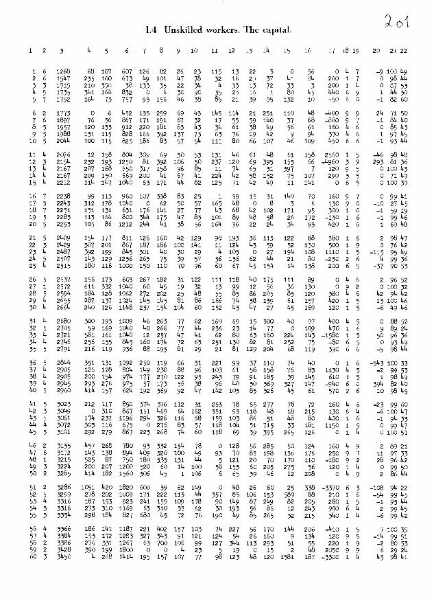
1.4 Unskilled workers. The capital.

1 2 3 14 5 6 7 8 9 10 11 12 13 114 15 16 17 18 19 20 21 22

1 6 1268 68 107 607 126 82 26 23 115 13 22 3 0 56 0 14 7 -9 100492 £ 15147 235 100 673 149 101 147 78 32 16 2 37 4l 814 200 1 7 0 98 1443 3 1715 210 350 38 133 35 22 344 14 33 13 72 33 3 200 1 14 0 87 5314 5 1735 3141 1614 832 0 6 30 90 35 23 16 1 80 145 144o 6 9 1 114 30571752 1614737579315614638 85213995 132 10 -5060 -182606 2 1773 0 6 1452 135 259 69 43 1145 1114 21 251 110 148 -1400 9 9 214 71 507 6 1897 76 6 867 171 191 67 32 17 55 59 1440 37 68 -880 9 7 -1 84 408 5 1957 120 133 912 220 181 83 143 314 61 38 149 56 61 160 14 6 0 851439 5 1988 131 115 828 166 392 137 73 63 76 19 142 9 914 370 14 6 1 97 445

10 5 20144 100 115 823 186 83 57 544 111 80 66 107 146 109 1450 6 6 -1 93 144

11 14 2076 12 158 8014 309 69 30 53 131 146 61 148 61. 158 2560 1 5 -146 9814812 3 21514 232 193 1250 81 392 106 50 237 120 69 395 155 66 -14960 3 9 293 81 3613 44 2167 207 168 650 317 158 96 85 11 714 65 31 397 7 120 9 5 0100143114 14 2167 209 150 669 200 141 67 141 2214 142 58 152 75 107 290 3 5 0 71 44915 14 2212 1114 1.147 10140 63 171 144 82 125 71 142 149 11 1141 0 6 5 010039

16 7 2238 99 113 960 107 338 83 25 1 59 15 31 1.140 70 160 9 7 0 99 14117 5 22143 312 178 10140 0 62 50 57 165 148 0 8 3 6 130 9 0 -10 27 14518 7 2251 151 131 631 176 1141 27 77 143 68 142 102 171 95 300 1 0 -1 59 1919 5 2283 113 1614 800 34414 175 147 83 101 89 14.8 58 26 172 -130 1 6 -1 99 14620 5 2293 105 86 1212 2144 141 38 56 1614 36 22 214 314 93 1420 1 6 1 69 148

21 5 21409 i14 177 811 126 160 142 129 98 193 36 113 122 88 380 1 6 2 98 14722 3 214.29 307 201 867 187 186 100 1141 11 1214. 143 59 52 130 500 1 9 0 76 14223 14 21487 392 1.99 8145 301 40 30 29 14 105 0 27 1914 108 1110 1 5 -115 95 1421452507 11431291236263753957 5613662 144 21 80-23026 14993625 14 2515 180 116 1000 150 110 70 96 60 67 115 1514 114 138 200 6 5 -37 90 53

26 5 2537 156 173 603 267 182 31. 122 111 118 140 175 111 89 0 14 6 2 96 5227 1 2572 611 332 1040 60 445 19 32 13 99 12 56 36 130 0 9 2 0 100 3228 5 25914 1814 128 1062 272 202 25 148 55 85 86 205 85 120 380 14 6 142 914 14229 14 2655 287 1.37 10214 i4 1145 81 86 166 714 38 139 61 157 1420 1 5 13 100 14630 14 26614 214.0 126 11148 237 1514. 1014 60 152 143 147 27 145 169 120 1 5 -6 149146

31 14 2680 300 193 1009 146 263 77 62 160 69 15 300 140 97 1400 14 5 0 88 5232 5 2705 59 169 10140 14o 266 77 144 236 23 114 77 0 109 4o 1 6 9 89 21433 14 2721 581 161 10140 12 257 147 41 62 80 63 160 2214 1143 -1580 1 5 50 96 36344 14 27146 256 155 814 160 1714 72 63 251 130 82 81 252 75 -80 6 5 0 93 4935 5 2791 216 119 936 88 195 81 29 21 81 129 2014 68 119 390 6 6 -5 98144

36 5 2814.14 351 131 1092 250 119 66 31 221 99 37 110 714 140 0 1 6 _51#3 100 3337 14 2905 126 128 8014 1149 230 88 96 103 61 58 158 76 83 1130 14 5 -2 99 5338 14 2905 200 i14 9714 177 270 122 95 2143 79 91 185 39 1145 610 1 5 1 98 14939 44 29145 293 276 975 57 173 56 38 96 40 30 369 327 1147 _9140 6 0 3914 82 14040 5 2960 4114 157 6214 192 369 92 47 1142 103 85 326 145 61 570 2 6 10 98 145

141. 5 3023 212 117 850 3714 376 112 31 263 78 65 277 78 72 160 14 6 -23 99 60142 3 30449 0 310 867 151 1469 614 162 351 93 118 48 18 215 130 6 14 -6 100 147143 5 3061 1714 237 1196 2914 326 116 68 159 103 86 51 148 80 1400 1 6 -1 91433144 14 3072 303 116 675 0 276 83 57 118 1014 51 715 33 181 1150 1 5 0 99147145 3 3101 292 279 867 223 268 714 60 118 69 39 395 265 126 0 1 14 0 100 51

146 2 3135 1457 268 780 93 332 1514 78 0 128 56 285 50 1214 160 14 9 2 89 211#7 6 3172 1143 138 8914 1409 320 100 49 93 70 85 198 136 176 250 9 7 11 97 33148 1 3215 525 87 750 180 535 131 144 5 121 20 70 170 110 -180 9 2 28 96 142149 3 32214. 200 207 1200 520 60 114 100 8 153 60 205 275 56 120 1 14 0 99 5050 2 3285 4114 182 1560 306 145 1 106 6 65 39 146 12 208 0 14 9 2 86 44

51 2 3286 1051 420 1820 600 39 62 1149 0 148 26 60 25 338 -3370 6 -108 914 2252 5 3299 278 202 1009 171 222 113 1414 357 85 106 153 589 88 210 1 6 _514 99 453 14 3316 187 153 923 2141 159 109 178 90 1149 87 2149 82 205 280 1 5 1 95 144

3 3316 273 310 1169 63 310 35 62 30 193 56 86 12 2143 900 6 14 2 99 14555 3 33544 298 1814 827 680 45 72 76 190 49 8 265 32 215 3140 1 14 -6 99 42

56 14 3366 186 1141 1187 221 1402 157 103 714 227 56 170 1144 206 -1410 1 5 7 100 3557 14 3384 153 172 1283 327 3143 91 121 124 514 26 160 9 1314 120 9 5 _i1# 99 5158 2 3386 276 331 1267 63 700 106 99 127 31414 113 293 51 55 220 1 9 -2 80 5359 2 31428 390 199 1800 0 0 14 23 5 19 0 15 2 48 2050 9 9 6 29 21460 3 31450 14 268 1414 195 157 107 77 98 123 48 120 1581 187 _3300 1 14 145 98 41

iE1!dI7 qL sialpoM VT

) ()

4498 9 0 Il 00? 69? 041 4t 44 L 60? 61T 6). 999 009 0981 69? 44i 11649 4 LT 96 4- 4 o6? T4 44T 411 L9 99 IL o4 64 114 90LI 1:0? 94? 9LÇt1 611 9T L9 41- o 6 o4 44 06? 49L 941 9111 94T 94 09 6Lt1 69? LITI 94? 994 694t1 Ç 9 6t1 6L 9- 9 T 094 9? 4o4 66? o4 ?I ot 4 96 49 699 1190 9911 999 60411 4 LTI

9996 9- 1 T O 9L? 9?? ?T9 44T TIT 699 49 o4 9611 904 4941 4 099 8L1I9 T 911

9396 41- 4 1 o9L- 4 09 94? 99 191 964 96 TL I4 TLT 9961 19? 664 91911 9 44 oo It 6 0491- 9119 01 099 94 LO? 000? 1194 990 9411 08 0 ÇTÇ 906 0199 1 911

4946 6 4 6 009 99T 601 994 1111 411 L4? 49 860 8811 91T 4460 460 44 40911 11

4466 0 4 0TL- 90? 160 9oT 4). 699 06? 04 L4T 999 604 444T 91? 84? 9L49 9 1111 9396 9 4 4 09T L6? 94 ?TT IlT 941 06? 6). ?9 6L1 1198 04?T 44? 1189 0949 9 ITT

94 66 - 9 T 094 991 609 401: 09 9TT 064 OOT ITT 469 991: 449T 30? 494 4349 4 OTT 59 96 ?91 9 9 019 491 44 94? L9 ÇLI 69 L4 49 469 44T 4141 44? 649 6149 4 601 04 66 41: 9 T 044 81? 90? 999 OT? 90T oL4 T9 o4 L9I L99 4491 ?6T 804 9999 4 90T

4496 6?- 9 9 099 60 44? 991 oc 06 194 49T 99 904 994 9401 09? 1169 4499 4 Lot 09 ?L 6 6 0 9 L4 69 94 404 46 4oT 09? ?9T 090? 694 994 49119 9 901

L? 66 ?T 4 T 0960 941 4T4 994 T4 191 OTT 69 44 049 409 8119 L4T 444 TO?9 9 401 9394 Ç 6 0 1141 L9? O T4 OTT ?T 88 ?L 0 0119 9ITTT 409 O?OT 9619 1 901

9T 66 991 9 T 089 94T 4119 L? T9T OL 9? 44 34 60 901 L?IT 4L4 499 9419 4 4ot 99 06 41 9 T o4 o4T 96 9L4 T9 1:9 49? TOT 601: 9191 104 9116 ?4T 999 4Lt 4 901 4? 49 T O T 08 69 441 91 041 lOT 644 94 44 69 09 046T 044 314 9419 11 TOT

6946 o4 4 T 0494- L?2 6?T 696 9L 9L ?LT 16 90T 449 949 IL4I 441 9?? 91119 9 001 44 46 LI- 9 1 001 TÇT o9 LL 90T 091 i44 99 49 9T9 Lo? 0901 19? 489 9?Tfl 4 66 60 OOT 0 11 6 o 04 0? 0 41 0 09 3? 0 04 0941 4119 1i?4T O?T9 T 96 93 96 9- 4 T 094 444 o4 6oT T9T 691: 91? 94 99 69 909 0049 99? 194 6609 3 L6 94 4 4 4 T ot4- 1191: 39 Tfl? 001 49? 494 9L 960 1194 oo4 096 ?L? 09? 9609 9 96

04 96 1 9 1 0191 L8T 946 L6 99 46 049 oL 98 94? 64? 946 ?9T 969 L4o9 4 46 04 L9 9? 0 1 061- 699 941 ITT 94 060 4L9 4 3L 604 1? 0491 LLÇ 194 8409 3 96 99 L6 4- 4 T 091 9?? 94 Lo4 69 T41 6T4 96 ??T 449 41? 609 ?L1 61? 9409 46

9996 4? 4 T 0009- 46? OTT 9116 T4T 60 409 6L 98 444 991 4Th 941 L).? 6909 9 36 T4 66 04 4 6 09L ÇLT 901: 416 46 9L 99 49 411 0?? 491 0409 90? 094 6T09 9 16

44 66 4 4 T 0191 TO? 88? 9411 14 4?T L9I 14 991 994 99 991T 04T 94? 8664 9 06 94 L6 1 9 6 049 ?9T 904 494 94 46 ?L L). 9 T?9 909 0601: 6LT 944 8464 4 6 49 96 4? 4 T o49T- 461 09? 094 T9 99T 494 49 66 699 36 949T 69T 99? 9464 11 88

9449 44 0 T 04? 90 460 1144 9 44 9 64 961 96 4991 141 461 9694 4 60 44 66 4 T 014 9?? 09? 04? 69 901 444 ?? 2.6 91? 949 81199 44T 94? 9984 11 99

9? 66 611 4 T 08 lIT ?T 96T 96 001 90 099 99 TL? 44T 0691 TT? 949 9184 9 49 49 96 4 4 9 o4 4111 ?6 OL? 99 14? 44 0LT 461 409 ?T? 0909 L4T 969 1644 9 99

09160 4T0LT 94144 T4 9 089446). T? LT?o41oT6 61? 409 9944 948 39 9L 41 4 I o60- T8T 61:9 994 04 191 949 49 69 369 89T 368 991 99? T?L4 9 99

6449 99 4 00090 941 449 o4 44 44T 094 911 44 004 9L? 4601 09? 919 9TL4 4 T8

04 49 4 L T 00).- T6 9L 044 09 69 094 69 68 994 1141 ?T9T 6T9 OLT 4144 9 09 94 66 o 4 6 099 499 601 494 09 TL 414 941 96 40? 604 1011 ?9 01? 6694 64

9966 99- 4 1 090T 1191 44T 91:? L?T 441 941 94 96 89? 994 146 48T 644 9894 11 8L 4494? 0609 96 o4 9999946 449 69199 9940T4004T 909161 6494 9LL

6946 94 o 6 0961 9LI 69 64? 69 T9 L6T 6 ??11 64 946 641 1194 9494 4 94

44 60 TOT 9 4 0441 69 44 91? 6? 94 171 6). 4TT 460 o 446 069 949 604 Ç Ç). 04 00T 0 ? I O?T TIl 9T1 00? OLT ??4 0 94 OIT 946 4?? O?1 0 0 9494 1 60 04 96 ? 4 1 094 691 1:94 941 3? 94 T). 19 99 64? 909 94?1 991 181 9494 60

996 ? 6 1 04? 60 04 699 0 L). T4T ITT 990 469 0 086 091 49? 9?94 4 60 9446 ? L 6 09T 99T T6 914 94 ITT 41? 94 OOT 649 L?1 481T 119T 94? 6194 9 IL

39 96 99 11 9 06? 909 44 ?T? 94 46 599 941 44 681 00? 0OT 0 0 9094 4 OL

61 18 991 11 o46- 691 814 6?T 94 99 69 ?L TL 144 609 9TT 104 4601 9094 4 6 34 66 11 4 9 00? 1141 09 99? 84 441 46T 0111 T6 699 494 940T 94T *91? 9944 11 99 84 66 4 9 T 06? 44? 99 99? 89 99 99 93 66 094 60 0*911 641 6?? 604 4 L9 09 L6 1). 9 T o44 231 4 4 09 ?9 *911 84 44 604 4TT 0090 TO? 914 9944 4 99

4 96 4 9 9 606 461 44 444 04 60 699 99 60 hOT 49 L?I1 991 L4? 4944 4 49 49 66 6- 4 oL4 961 L T9? 99 49 ÇTÇ 96 94 949 1911 9441 60? ?OT 4944 9 99 44 66 ? 4 T 004 T81 T?T 66 *91 96 06 94 ?9 644 L61 0991 191 089 9944 9

4996 T?- 9 6 039 941 401 TT? 94 ?6 01 49 48 960 161 9601 441 L 9694 4 99 09 L4 o o 1 091 99 4oT 999 L9 69 4L9 991 111 999 LI 6991 TEl 6L9 4994 4 19

60 T3 03 6T 9T 49 91 60 91 60 ?T IT OT 6 9 1. 9 4 t C t

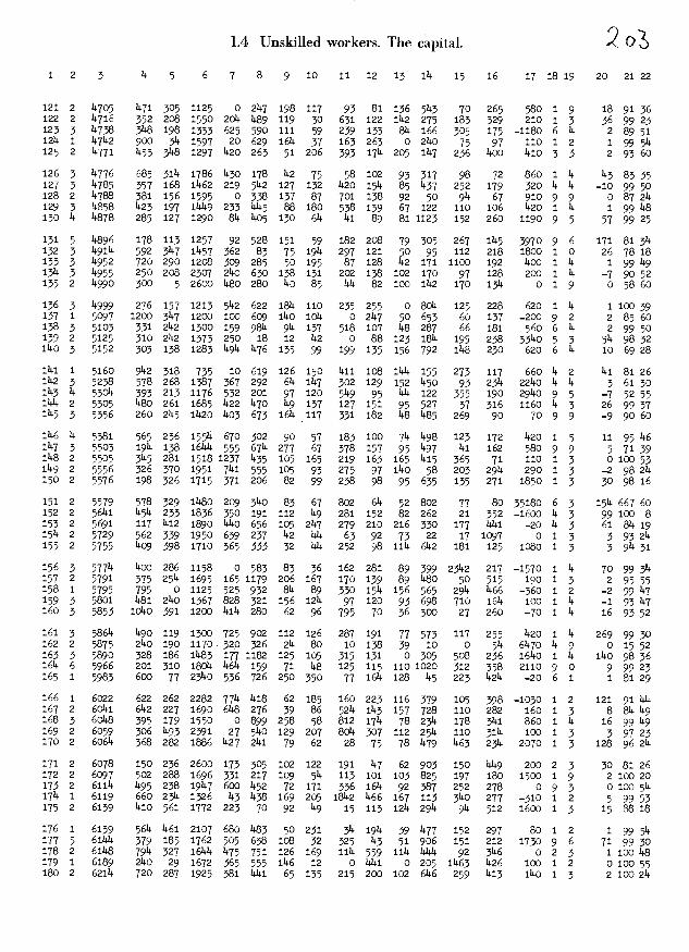
piidizqj sio pjjpsuI

13 OCT 34T0114T1j6491193010024T244T49T198Ç426TL93 03L11292O9T44 OOT 02TCOT931j491T4030TIlh0319liTG4943L9T63o168T9T6L12tj COT T43O913611ttjITT64ITT69193TT4L4Li119TLgÇi6L9111938LT04 66TL96 OLT3T314T906T44iGOT 89 40439LT49T6L1T11194LLTI66T3109L63341LLi6c16T1T4304Ç911099LCT3T9111946419T9LT

8T 994TT009T3T4161631314T1416136OL3LLT1940Th6Ç1934LT44 6643To14LL3oi4ÇTTL9T9911719140369T941jÇ1197T1j470996TT9ThILTICOT O46o8L3L943619T9ILT3L341i009L161 93 46i11T974LT03 OCT 76T004T08TL613840TTOTTT60TLT3T44969T993204L93L193 19Oc003611T04T40629LI16T7713014044LT0093943O4T9L093TLT

113 9683T41oLo3tÇ39I6L18L4L93396LT1jL7198913978941190970LT4L644TCOT114OTT1473TTLo4 1O9Lo363T014L7T64346190464093691611669T1T099TIÇ9Lit3 8LILT3T884943669oC44T6LT46491109489T61 11994109T393OTT83LL41cIT1?499649L39190691L7331j9111093L9T11t1 16T317TC4OT-96440T6L49TT42309T491399T1j1LL39373933393309199T

63 T9TT907-171133I83119TLL044 04392L9440sÇ7LL0094964149Tcg 666o6OTT79443T4O3OT OTT4TT43T911T!64T119111091014TC39964919T94 96OITII01j9T9439044040T414T440T43T791T LLI491iT99T934o694449134 4To61oLI91OOT6494T010813924034 OLTIo6T0134L243391o6669311T03144gLIT4L4LLT6TL9793T311 æ6 43L00416TT06119844T91

34 469TITCL-093L300494OL46L963908311110031164OIOT44944O9TLI 46T-11COT191OIL96946O3TL6131941T24939L94T013T9t1T084c64TLI 663-31094-99116349494T14T0446819346434431To46L46L4T94T44 464T06T4T404ogsi6964ToLiL919036LTT 49T469T 13 4L4T6L47L4T1166CLII0L4T-LT33114366469T9279194484940941T993CO1ILLÇ494T

T4 1644T090142TT8T319ITTT963431974ccc494OTLT96460144L4344T13 4644ToL6oTLI734L36491931L47649o46i6439463L4314T61 119T941C7-T19LLT0449T30T36L3L11g4oT949C19 06917ThLTTT694344T9COT 6641CO9T344T33973974TT97613TTT61044949T447 1IT194734T09 L99 1414909T4409LL3093419309L949014603081T6348L46L443T4T

91 860441o49i1L744T44946969436679907TLÇ4TLT9748619L443o4T12 967-4T06311674079401I1L64L2464o1444TILT461oL4974944436IT44 COT OÇTOTTiL494'i49T49T6T249140T 41 L42T 9T4T19241144044791T64 IL46609479TTIL6146L419L4L9LL71L9444119T94T16T40444LIT91 46IT4T0317L1431961ILOCT49TLG06304oL9144T94349419441191T

09 06 6-66CL06697918.179T144LIT19T4L94oi C3IT411209394444L4 6693IO9TT914L4L3446T41L7TL4T61oL1331499TT9709114o4471fT444L-460162o6T44473T19466114C3TL61027449LTT4T3 464ioÇ4IcIT04 T941101771424604124T63T204LIT19267L94 LT 9979L4943441T97 T9T171099LIT4L?44TluiTGOTTT1104193T619CT44L914316C9T4TTIT

93 69CT19039043GIIT26L94T44T661664419Ltj161 483T94T4043414401T34 86144014494246T19T471990312T9To4L4T711g0T44T4g64T04 66Z1909T9199L9391LOT2T4L4T16i6 64T004T217T44coT449cT094976003L4T0949 OL12Ji10101T609OOT007TLIc003TL6OTLcT64 OaT TIT079824T1i0904424OTTtl9T3792IT71 LT 9L266614 9I099406ToTOLTITOCT79tt4901 070ioo9g4oo066174I 4 06L-1100787TL6oLi70T841207T4T94T 09 O1Lo4290704744611T61 66T1T001761OOTTTLT2181 L946T04226o90T 06707L746142T 9L9OT009T8T7ZTT6oT2TL621614L42394L4IITLIÇ761T6141T9TLI96oL6441TL94046Lo29T6T4T976L47T4TT8LT968t14IÇT

66L446061109GT2TT T969TI190410I12o6I LTÇ99L91iI 911 66T1107190TOTT3T1364T944OT4+i6*tjTL6TÇ71948t1Ç 6T12L8066oT6L916069ÇTTOLL9L41 94406I9TT9Ç89L193To66OT-IIO6LT42LÇI491T 0gÇTL713I6T9IT99T L449L1Ç

48IIT0993L86LT460T94LI8LT041199LT1TÇ4999LLI497T

09 462440T100194LIT407ILT90gT49031L67T9IIÇTLLII7t4 661TOTTL6L0130Ç949TL41916g9oL64T1oo6711L1TT6219O2TT-4LT99T1184T6TIT0647944T96191494L1447 669Ç410T3674c2TLz1iT7T149046T16ioo4T 907449TL194 T69T6T02449OL41494TT946LTT96TLo7TTo4TLI4oLI7TgT

77 T3O?6T 2TLI9TTITTTTTOT69L9414T

09 860T90016149464911 L9ç014il10t1144191kL690446TozL164610111

till L6lI110901-9P4991szLT ToI69190906108169L11940041ÇÇ4991616cz114 66 1-Ç604).LL199111641L4ÇÇIT4611Ç1L91 11010461194L41T4Lz6186141 66ç1909491111Lz44441 11119410496Lo969o8L09410440991099TLcl44 661190191949946146166116L9444911911 011441L461919L91961

09861114T009411L914ç66100111660191LIlT 4L9011141696111999146194 66L-1106499110989441101919841661oo9141409LI).Lz99T114161 66TT9099646164111614L1191ZTtill4994911 40910119L094914c1Il 461LI04616994L191L81L61919110116L1O99L1119181111448T14101 681146o11Lz9L494).1901 691TIl44419OfT9L904404014910T99149Z14?

99 001 19-T4o6T9T494944otOt60091lOT16606001109101469991o4z94 f6f-11011419OL19611 IL1111149199L14409).091116101014099T6119T L6141Z9o4-46161119900419L911191119L0991 411.114LL11188T8181104 660110994491L641 89169T011901IL419119119411496006IIIT8TLll11 001 Ll41019964401996T 94149T91666TL004149L19149T914f6191911

46 6691Z1019T- 69Lf11L4o1 111116169916iiLL191111 914Loll6149069409T411f4 199111101991LT4t4619994696).L9941?4t9194101994414496f6911Il 669T410611L4446lilT491691191141LllT 91.46411964944496).141161 1146 619000flLo94194449LlT9099101149181116141 0491644699oz6LT11194 09L-110019444o49lIT11141L10119610001461L4649).TIll94 66oIT09994014669T 991141644091IlT999944019196194916LLT01109 IL011110914991909199999994oLIT19091011404109494LL161144 001 91110911-Lo4T8ÇfloT 11111611101L1T9114401 41foIl616906699L19T104 96044T0111-961t1L9464661616941911111949o6L9L61691LtL999).1LIz94 664-4T0114196loT6001 6119T144T494919161994111L6zÇLli949LZ911

f496 Il41091-LLti04TLo91419610961149969L0414zfT6fT104199L1411i4 960441004404011991441ILT614OLT96199IlT46T1491oo40T9L1911

t1Ç 001 111019841104L44411191Otil14TlIf4ToL46T1449644I4LT4116946LI4T01L44L1916496699T1096t1090491L499111444Tz449fZ11144691-49014044991zoL001Lo44446L499t9490441012094TTIiL1IT1

çt 66111 o41419OT44L919L9Ill691.0991+1O0l9694L60111fTOIlL9 OOT 4949oii6499T191014449119014ZT19094049119Z49914o9L16oz

661941099-t1191499IT t0T94164191L9T9999L4001041 19TL1Lzoz91 66611099T491T119111 4TT1LI99To640?L990140tOl1169ÇTZLZLo91 66TT6T09461+10IITZ691414991641041I114LCOOl1419Z4L0TLZ901

9186TZT0146LI49116LofT11T94fLOT1919i +49TZ16411Ç916OLI0Z94 661460611114L11z46L11Ç1allOT6f041446tIl1010141801zi06 661104164140011Ol6449T141169T199961096L491T1+iL0LI114 664TT011lOT11944904ç4t09190449OltOLT 041ozLI0f11016996-4ott-4640011149491 tI 0044919L9Th11949I9Z f44410L1TO

91 99411109L69010019114019111L64ot4L0660041TOl4996991oa?i46o11091L914i94Z14L9 oo0LT11TIILÇI ooLoft1l91Too6999661

64 f611TT01f-Tt49161II9L1416L19fT119T60990191994049999T6T

94969116T099441469194111TL664T1LT641.44LI4Ç9T0l9T461L9ZL6T

0496611091-Ç9t401Lo4999 944146+9011664991TII6T1?11999991961

996-49oL6919+IT49961991641zL4TZL49t4410111Zt9LZ69916T111 661tIO914419011091 94L614699lOTL194z909l99T941Ç99696144 66oTIo1901)2691491640181TIT46101L04o0141199T46114 961(9000T001664o4ii9T14019f16I 961419469LIz 001916969Z16T94 001 060411111Lf1194L6LZ19104L14961901f 9600640Çt6Ç949T161

96 T61110ft-994L19f14694f911.91lii9014499TLT199944949T06191 66990414040909l6Tt?Çl69199tOI1Z4o469c6c9446Ls9T691IT6L64ÇIo6tj004T4109901L4944111061+11110991!MII11IL8649Z98T41 t966-4t0Z96LL669T44119T1f4T69L44oT664L4TZTZTZ9g94696491L91tÇ 66411091-LOIL14L6LL9z441oL49Ç99T1499Ç000T9ZIOOTTL49991

cl 9616To4TL61tlI0t1ÇOT164T9L9lOI946cz91L991914691l9Z

Ll 66t11091o69600109l 0T91Ç911TI6oc4 oL09 lLII9I99T44 660190t11194094i4oLI001191911 oT O01L44Iz9Ç9ZoT

IL6t1Io4lT4f4ÇLIII941hifI911961191966I11L490110QoLÇ64z9ÇZ9T14 OOT 611o4z-L611iI44f41911019919911110911ÇÇ19Z dOlO1QT191

11 11Ol61ILI91419141lI110169L9494ZT

1ijidiqj SJJ)1JOM PJjpSUfl VI

1.4 Unskilled workers. The capital.

1 2 3 5 6 7 8 9 10 11 12 13 14 15 16 17 18 19 20 21 22

214 2 9131 371 325 1500 l09 891 212 93 912 267 150 1332 171 38 21190 1 3 121 98 502112 1 9t35 1080 1105 2500 1200 255 t5 290 50 100 liO 1700 135 382 250 1 1 3 96 3823 1 9720 960 112 2653 829 1036 171 195 37 268 200 1801 493 497 160 9 1 1 90 132114 1 9869 1116 608 656 625 1015 156 139 569 81 590 t76 110 1148 i1O 1 1 7 98 19215 i 101407 830 338 3100 914 1058 189 269 680 173 185 1195 1662 590 -660 1 1 16 98 35

2146 i 10856 900 814 3106 146 1259 122 362 2148 253 207 1455 138 1481 1730 14 1 -114 100 122147 14 111400 190 175 1625 259 1714 110 31 2814 110 73 86 5033 232 101140 1 5 126 27 332148 1 11703 814.0 56 3186 1506 7149 1140 390 130 299 14140 13142 170 586 260 1 1 14 914 145

2149 1 12061 11456 0 31445 669 1967 217 350 65 3140 1058 1270 100 51414 380 1 1 1 78 148250 1 12683 360 55 3120 18714 832 119 300 36 205 107 775 1235 214 140 9 1 0 100 53

251 1 161489 780 6 18814 80 528 110 155 136 1140 102 517 2140 136 0 9 2 82 914 1#8

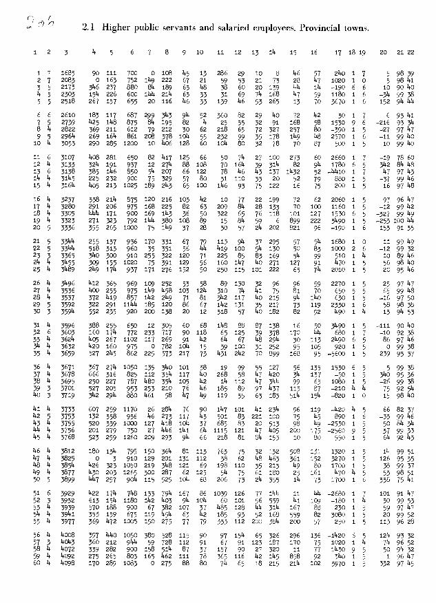
L63ccToL6cæi1113-39c911LogggcLlocgol69OtT96ot1Ij09Lt1 96TcTOt3689Çt113119TTc9c9Liii3911c9TÇogc93cLl3601ikl6

c 116o6octLkiloc Ll06LciLcL9t1i.c9ci006lg6ccLoi11gcl96t1L111OEOTct0LTL9TT6L9i690k6111161T109ccilo11cLcc c6icOl1T-9c196393c9c-L606l-91cogcocoi01111L690011119c

g96ciicTOtc003t1gcooec.c6kLLL3ocicooi1L1169ÇTLL6iiccc 66ocio9oc396c99Tcc6cTc9t1Çt16T1cL96cTccc1116c11IIÇ

Lt1 L66ccoc9gL91111cthI931cgt1LLoT19cL9oo6991otc6c6ciccc6 66cct091-601n169cTOT0911OT116cot131110911IIÇTcT9lc6cczcL1116lOTLi0991f111TT+1111LL91T6cci99L9T116kccT911!liLT6z6c9Ic

TIL9cc91cOLTcLccck90399IIOTdccil1i06LczLi1t1669Çcodid g6cc110L11T9109119Lidl 39L81oocc9zTcoloÇ11LLBcï611L66gccTooki09611cIlOIT96T69T1T9tÇ6T1ocoi9ll11Ç9cicc691TcToklclcT19cc911913991TTTcTTol631016çoccïLilTd 66111dToldTÇTgodldTcdLc9LcIlT9119cOcTd6L11ÇT091ZT9Çt911

ci1 36119Tod09OTcc119T99T199116c61603091T6dz dcg9Lc11dlicc 66Lc6c9cl-dLTooeco11L11131cTII119111191111klocL6L11039L11i11

11c 1i9odciocdl-61196dc 03cgcg9LdhOT9T11L1T000T6ddolcddLd11c11911 66cc-i06g11L001cgiocc11LITcLl9119c69ccldTcccc311Ld 39c110311-6cr9611c3111lOTL111069L119?93OLTT6d1L09cctc11111

011 96clO1039-11d111TccgTc9cc611611L11gcT911099116311c6TLcc01111d 36L11110T3kgcTlkd11L66gdgi9119LOT1cczdd6dolLlcToLdc6cgc 6691-c10901c966itcL111TT111311coi11cc0911kgLL33 ozc69c119Ç9c c6ct1ÇcToc-ci11c0311L11gc993011LTT11cc1TIclg9Tc999gL9d11tcgc 66ccoccTcci9cL3Tcc666TgcTOTot1cccTodoT11L3L9cTL9d119c

Ld66c3ci009c-d69916690k3111TdlidLtIlctcdl?399ckllLzc6c9c11ççgc66ocio6colc63clTc i6cdlIiOT39LOL6O9T0lf3d9i1tÇ911 L699c06113cTToc1163911L91191i16693LTTlollL91cokl1119ciccgc 36OT-L10891111OLTgLc6ddl c99TT06LTLcdZLL11LT09Tco9c9lc011 06ITT-cIo6t1doc9Tgciiggi8909coc31o9cclggc96cc11Tc

cc116cT11106113638381011tcgic3103gcT003036ccl3cc116cccoc gc 96gc9TOccl611cLLI3ccTdTlilTL999031cgl 1TT T61llc16cc63oc L69Tcioc90111116cIl011LIT311cT9IL6113lliTLcg6111lLctccc1193gi1 66c9ccoc9OLT9ct11111koickllTcolgc11611TL6ccl00119cccik11 L6clciOkll69696lcOcT6ggÇcc3d696c9c?T119611Ç1193

911 d603cTOTO311Lc9333TOTciiocloczcT9LlILT L611LT61136911c11

011 969cci0L1116thILl011L1110919c631T6ccL0301ccl60cccklc11113

91168oi11iolc6611c691cgcgdlILOITlzcccloi6oodoklcc9ccÇczlc 663T-93cOOTc9odocTkldOOT6111trtl9c1cccc096dc 81ctddç611 661101099111Lc6lLd116cIT6).L91ccotT9c6LcTccl1111cccIlcc i6cci9o6T-96T3830311cocgtc611Tct0001c91ccc9ccccoz

001 cd-cio6klc33366g96118ci6g90Togc11Tl6LczcILldcc116T61166Lld-coccTL3TTOT91T9Lc9llcoc9cciT691006ILTtt111cocc119T311 6631-cTO9TTOOTOLcci8311860?c939czz991L6903163ogzd11LT

kil 96L6cT0903393k6613?LkOT311oT913OITctg111?gcdLczc1191

811 L691cTcclL9T331kc6911T001c9ckll69TcloTcTlcoi119Tc11cT911 66Ld-c10986L3dOlccOTTT09tc6zcct006zczczzciTc11liTcli L6L11LTOTl-3dlc11TLcTckl9119k33199tallicocg9111cgcgcicci911 118311dd9O9LT1161glicc1191OL90Tg11L3liL6161113cccTc11IT09 2k61-L1099309cL?OcTk?11koc99dITLT1139oc91839011Loid9TT

0116601cToocL9OL9k3d091101099319011010031cgl063ccoc1101011 66TT-9ToLd3go61118LTcc66ldlcctIOTgLc903199119169311963c6L11 L6kl-cTo6d-ogLdzklchtd991339oc3136L319TT?69c339319kldc69T?-96odd9d991163ddddl11zgd6T119dL990T1116cLzcL

11169LToc3113k0116339o9c3d116dklÇ66zL99LTTc91019?99

1111 116lcT9ToL9cOLdTc93cc9116c1cc91191103dd9LdiL9391d3cc9d66lid-9109TT6cLi99111L69cccd911131111100993?11d1ccclcil 011 06OT99061-liT11116cTOl099c911c96gT119098Lcl911cdk13ccT11 86doTO?OTkil93dLT?cd6dTZL93336111zcLd91OdgOlL36d 96cLT0113Ld9119OT6?99?dld11901000kITT06d991LT

33 13036T 91LT9TcT111dT1TTT0169L9c11c3T

sUMO ppu1AoJso1dui pJiqis pui SU1AJS DqqndTJ

SUA&O1 11DAOJd s(o1dui pnnps pui SjU1AJS zn1qnd I

ic 66 4L Ç 6 oqÇL- tj9 olq Ttj 4L ILl 646 001 LoT cloT 06 0461 mq o LTL4 1 011 09 66 6 q i oq 411 LL 94q 64 09 tjT9 401 66i 44L L94 ooLT L91 LLi L4 Ç 6u 46 86 60i 4 1 006 08 1401 Loq ou LT Lo6 06 L4i 096 q04 L90 61 0 9994 q 811 14 49 801- 9 1 0191 96 49 49q 6q 491 LL 60 601 L94 661 L911 6oq iLL 9044 6 LIT 9q q9 1i41 4 1 oOTq L9 æ 604 q6 991 19 6 tju L96 941 04h 604 4 1L44 9 911

4666 4L q i o9i 960 6ii 491 98 101 44 60 o4i 096 8 ooql L90 991 44 Ç 4u 66 01 tj i 0101 q6i L4 L4g 19 411 19 911 99 199 691 LL4i 44q ooq 6o44 6 0446 94 9 T 0664- 6m ogu 194 49 411 181 811 19 iq4 o41 009 944 1LL L9q4 Ç cii

Ll L6 q 4 T cou- TOI 91T 4L 41 44 91 041 41 181 041 LÇqT Ttj4 161 9qq4 q 111 4q 16 L91 q T 009 98 91 906 44 86 14L 9L 9L 994 991 1101 Lqq L9L 4Çq4 Ç ITT

q4 66 69- 9 1 0901 OL 66 096 qLT 401 104 9 06 qq 961 4qm ILl 496 0644 Ç OTT 09 69 414 9 T 0611 qÇi 181 096 941 101 069 461 901 101 011 0411 091 991 9LÇ4 4 6m o4 96 96- q T 091 401 666 944 4L 941 441 qc 09 L94 49 646 994 ooq L914 4 901 91 t6 161 0 9 0961 IlT L6I 94q LIT 611 841 14 401 111 691 o441 144 49q 9414 4 Loi 16 66 tj9T 9 1 0411 011 4i4 Tq4 64 19 941 94 141 194 191 4911 109 16q 4914 4 901

4Ç001 q6i 4 oÇ9L- 911 8991 649 L9 91? 994 L4 IlT 149 091 4901 411 960 6604 9 4m 9? 66 499 4 1 oiq4- lIT 9L1 L41 94 09 119 901 19 IlT 011 0011 699 t1091 9914 q 901 96 66 901 9 q 049- 401 4q4 oLq q4 401 LL1 69 491 0L9 91 1441 911 0 4914 4 401 91 66 o6 9 i 0641 011 14 oL4i OL 6m q4 LoT 901 91q 909 9901 981 99? 91114 4 loI 09 66 66 q 1 018? 911 4 901 6LT 611 904 66 1? 009 994 0101 LqÇ 144 46o4 4 101

6? 66 q 4 T 094 qq o 4401 601 461 Ll 401 491 964 9 616 oil 091 9904 q 001 84 46 411 4 i 0491- 16 Çqi 194 16 q6 649 9 46 6oq 04 0011 914 9ijq o4o4 q 66 9q 66 91 q 1 0911 111 L4 qLl 441 loT 461 6L 9L 914 0 L9ÇI 4L1 L6l q104 4 96 46 66 9L1 4 1 0111 401 06 669 411 66 oÇq 49 oLI TL9 11 199 Lgtj 611 696q q L6 14 96 4 4 q otjÇl- 66 L1L tjO 441 46 q94 401 001 184 904 6141 611 4q9 4L6q tj 96

4496 64 4 T 0LÇÇ 441 911 LL1 9 98 114 i4 961 494 001 o4oi 901 L14 6o6q q 46 lq 66 09 9 1 o44q OL 4691 966 14 001 909 101 Ill lOt1 191 916 161 4q9 T48q 4 q6 44 96 LIT q I OqIl f9T i6 6L 19 46 IqI L9 64 4i4 44 0411 01? 999 tjl9q 4 46 4? 46 L4 tj 1 041- lOT LL 941 9? 09 94q 1LT 14 49q 001 lILT 194 o6q 4969 4 16 66 19 649 4 1 0111 L9 19 666 89 66 9qT qci 99 cq4 004 016 414 99 l4Lq q 16

14 46 ooi- q i oqLÇ 19 04 161 14 19 911 q4 9q 911 491 4L1I 114 044 0169 6 06 04 66 LI- q 1 0096 i6 6i 111 L4 6L Lcl t19 011 499 001 0011 411 Ç9q 9ILq 4 6 9q 66 q t1 T oq6l 09 66 1lt 69 L4T lI 061 OTT 4cc 0I LqlI 191 qiq 9oLq 4 99 14 96 411 tj i 016? IT 91 66q 4ci TT 421 l q9 4oq 14 0001 ILT 9tf1 9699 Ç L9 q4 L6 TOT 0 6 oL9l oLl 9911 491 91 44i 141 q oil qLT 4oq 4oTI TIl 16? 1999 q 99

qq 66 4T 4 1 0941 941 0 164 199 L6 4q4 46 T4 66i 4i 0401 L9? 66L 0099 q 49 4q 06 6- q T 0186 911 9 691 18 49 94 4q 46 qÇT 491 000T q64 oqL L64q 4 qg 64 66 4- 9 6 0161 09 94 066 46 OTT 191 6q 911 199 411 4901 OT4 cqq 6L4q 4 49 44 66 91- 9 T Oql 99 9011 901 91 q4 44 qL 16 L14 4L 1191 6Li 641 9T4q 4 19 9q 66 8- q I OLOI 6oT O? Ol 4L LIT 04 t19 46 q44 ooq 0941 914 Lo4 44qq 4 i8

4q96 1 4 1 0991 6L 901 L14 lIT 911 941 coI 601 114 161 446 414 949 99t19 q 09 4106 16? 0 T 0949 4?T T9 464 14 06 4?L 91 III i64 191 111 lI L9 4qqq 4 6L

04001 99 4 1 011T 09 944 64q ci LIT i4i q4 491 u4 441 449 191 004 11119 q 8L 14 66 4 q 1 099 q41 09 qIÇ L9 q4 401 66 49 61? 01 4Lqi OL? ooq 80119 4 LL

1466 6L 4 1 o4L q9 q49 99T 4? 011 411 99 lIT 61L 091 199 941 6i4 194q q 9L

01 99 491- 4 q o9qs 94T 11 941 4g L6 æc Ill 064 T6 0901 L14 Ç6oi 646q q 4L 44 96 601- 9 1 o9q4 LL 041 641 09 49 494 qÇ 9L LL4 091 0901 91? 1L4 0949 4 qL 44 66 o q T oq LqI L91 94q 14 q6 141 9 qL q94 461 096 441 094 644q 4 4L

9186 911 0 T O?l 411 4q ILL 44 99 49 6l Ll o?? 161 oq4T 141 494 6919 4 ?L 94 66 19 4 1 0966 06 09 1L4 141 06 19 96 911 991 9T? 199 Lo? i64 L919 tj IL

19 66 Ol 4 9 0LL L q4 061 14 o6i 4oq 69 441 LqL 491 4L6 141 644 l9lq q OL

qq 96 91- q 1 0901 4L 01 9LT 66 641 4L L9 691 9t9 Ol? 0011 9Ll 914 9Llf1 4 69 44 66 4?- q 1 014 66 44 OL 911 9LT 996 l6 91T 611 09? 0001 19? 914 9911j 4 99 44 66 LI- t1 q 0111 14 941 16 LI 991 466 09 4g L49 414 406 Oh 990 6919 4 L9

9486 691 4 T 0141 16 4h Lq4 14 T9 18 14 OTT 949 19h 419 604 004 f1019 q 99

iq L6 99 9 T 0044 94 9111 994 LI 49 4T1 64 491 949 901 499 qLT 6L1 1619 4 4 94 66 4L- 4 1 01191- 19 04 q94 09 09 641 iL 091 99L LL1 99Ç1 LIq 194 9819 q 9 44 96 911- 9 6 o66q 4q 14 191 Lq 49 4L1 001 9L 6i4 8qT 0h01 691 184 LLI9 4 49 i4 66 L4I- 4 1 0119- 4g 0491 4oq 4L 4L 91 49 Lq 60? f1?T 49 4L1 104 oLiq q 19

qqo6 b 4 1 oTq4 191 44 44? 99 ThI 41q 96 L41 4q4 LLT 46L 161 6q4 L4T9 q 19

lI Il 01 6191 LI 71 41 qi 61 hT TI 01 6 g L 9 4 q 4 1 1

SUMOj J1U!AOJJi(ojdm pnnqpuUAJcjqnd4!H j

09 66oi60649c111016411 09108116890494i0041 3+L0091009944æ1I0919i 9641ot6oT49TL46îL414630419014L9t1930043 99 64LLoloI36L139099941019kIl04194 64400106LkL4T049009o4Li9669694110139L1c66c4o3tÇ4916LTL9443139393141693cc4304333t14ç6kT1i6LL43 66c46094-LoT8kT49949909941144649649944L3T31k9L1T494639kT

44 86o03L3T64944T604Ic934131301ko63999491043L494614Lik9 664941069106134339601 4634619t631669940990041919304944639L134 99114910966181kL99490313kL6661100k00144)2oL3oo99446ç4Li93 394109111914194931 001ILT191ç41499k90614341999L94961633k11i4 6694-41o6L4001k9349L331969k4T9996443300414399011cLi63IkT

44 46T310191691461499L43193TIL699310911 6614061994936T6116TokT49 16kl-690Ç993691409046k839L4631okT4610994)20341o444L49906369109 66LI-39046OTT3910461 Lo3639999310419991 0031 0490099)2T89143 66LI41096013499994916L6491334T0640434L9334649664993k91496 4914T00998330936L344913ok3TLcT0434944o003149999966493991

44 4646901O3L4191TOT9411 IL91109T14491OIL0090091L699999049349T94 k9L9946036446109TL99Lo4T61OTT9999k43L991L4403014939399144 990634T0L499431849440661949909611094034190444439393491oc 6669T06931314130491 344LT649L96919901 9949)219136)29808639161 L66)2490911T934094oi9419LT00148080914o40944808919111083191

99 36901tT0666IL393306*9441914OTT641 099 64300019L40401L96k409149883334To39c6k99349k94493349TL9T1614031 390063436901496k964114 461614T04111639419L11 001LL3946019111460k939140904k998L394169 66413T019981oL46991 093094431619416960030091403k9k9kTk4169 6k6-91049139469911401 3439kk3311LL949991096893994919k4941

04 66064T0091991TT0131 64196L430934k4k9994909109964k64Lk344144 963346094-391446943k4ki349401999Lok94100416L1139ookk394134 001 413T014091099494081913491136633416044441911094699kT44143 48kT94041406911194o48019914k94994040491649Lo9399k334194 66t-4T0L4T3LTL91909LLTL9T9119k4986484k3003694419L49k3141

96 66691-0906039311314944kL69414696998049OOLT664ok9T639L404161 L6k64T016343300196914k3391440010460040061399L99309L369194 9694410499-991099-900010414LT0349138L99440041444099944k399103 364934T06434kT4LT99138001419096990010841369ok93L3L3L9T83 Lk3k99o4ttT91100819649934193L949904IL003TL49499691k4991

43 66039T09116139438303 L9093041914146k8033941L993649LOL449146 t64L1OT06644L91943909ILTk6961899930040903k93004940k999144 001 9834T099189401941446kL9TT4903L8493049193469014ioL349194 66 o41039496001L9603913009439991 04304k4k444ok69339139 9603-40669kT6)21948094139186191444k40031LL344k34693191

13 66444T08969106339964896k469TOTk9L94996k16k31t11194693091cc 69944T0904-931ILT4090966916443k3T9011 94134014L31649189364139 k61k4104441910499491LITo4c93k94910640041k960694699394104 6664410664-001TOTLL91304194k433110199k4936k3T44346939993L4164 961039T0109969L4L9L4kLk90T9kOTTk99004T9OT96T919T999494T

63 3934301039199919399119L96639499L30010066939940949964T69 6694-69039449T3LT993699999906994411okIT9036440149994109 6694T0993T4TL4T3494tiL4T441LB99314949343313996L4ok39344164 k649T9T043663L4)21 06633okT41199169996400913449999619434193964LT410963330414901T9TLooTL69410411060031Lo96463kT93141

99 968090T004309T041969TTk3T6916419910649994L6144k436909904169 96okT9T03819114091949414113606941L360034L3T1434949909463144 66kl60LLT491031k4314001603399019341196L9TL4409440094931L9 49TTT4T0944-06163349499L696444601944113030140901444649k319496 9649104640313440434Lk9T6LT1990194L94441604k4494644931

93 46BT-990949999LT9L34k0919669969999446)2L394999696443199969314T09936L4T93L93994k441L4Tk094391006313394108499319496 8896091-343646411 901161)299691949k9oT99T96464)2443194 9999101O3O49619k44199L9T9L9144464049194k9IL99949T64k6433Tk4 48893910393331449049L93119149491919693003190309994)24131

33 T3036191LI9141914131TTOT69k94943T

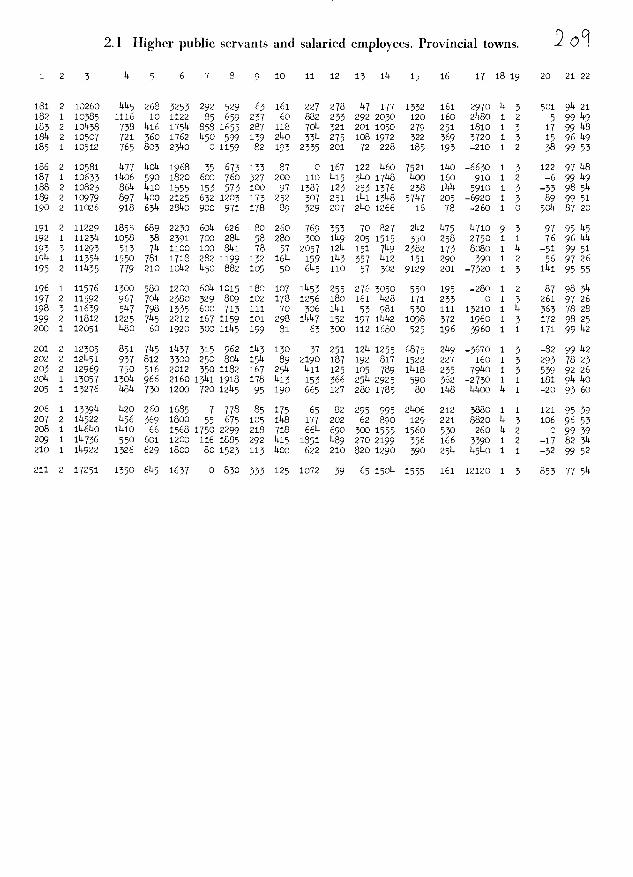
Qsut&oj pzu1Aoiojdupnjis pu SjUAiSjqndj

i4 LL46T01111T9144Tt04T 49661LOT4444o4oL6914t90441TcL1TIl

6616-TTotÇi1ti6064o6lT 0190119ooll411 44T o90091619914T61TToIlLI-1i06449919466611 oLl68114914Th161499T 91100111090469ÇL11TI6

64 66011091o40941444T 0040691999TL66æ O4LT 994199OIIT0119111T90144 969oT4o9i6i06919101LLIT4014L94oo9T6949Çtl4tI1Lol64 46IlTIT099411190l46646119494L149LLL4991091olIl1644TT901

09 46 o-oo9110949L1 091L1T699o6i464IT olL0011o4Lt91.14114ooil 16T8TIio4Ll-1960644161 1419964414119LT9161 1161 0911996104TL4oÇTT10191 166646T0161.441911T691.4oi411TIl1141L91191T 0441101914o4L69611160141 9L4614T0911.111141L19161L91o6Tl69114T108 041oc44119L66T411111101lI 669-6ToL94-61114L994411 1111141L6oÇi4111196414L411141L1494041T1101

li 66ILTIT09649614140991 1TT0046919661411T1 oo40161090911T4O1TToel41 961LT41096111.4860111thL611411.11111961lOT641T 1.9111114iL411T1T911166T91 9L49411T01141ITT044196441111904OLTIl611.009444i96LLi466911696191 L61916i0641ILl911119109194119LTlOT60961409411101.1.96164111L6i14 961.91T091-46i0440404 9L144164111LoT0914101 t1O9COlT09400419L4TTT961

44 46TiT4T014L-10161161041.4011119440119904111010116LL44111146191 L694110640611411111.4441164119T1416611 1919TLI191.04411144111116114 66T4-1T090941.11941611L14111111.401L49L1119001OOITilL41446111446i1111969LIT04L19410444i4T 401611100609194191OOL164194940T1141111161i 461.6460TLI4L1111111.19OL444691.09109919110904116994491611111T61

Ol L9iioÇOT091-91.919911 01111.01616698LTTL6oo601911Ç99T69101T106114 66694T0169-401LiL481141 TilT1411.0414141.14011 14941T10011.696L6oT169Tl9644-610T64t11l9619L4T 4416111.9411.600161.4641444101119941OT1 9T61 6691T01609T0011811.1 014411011001L14091.009019106490111449oT11.91911 1.611T410499-01TT14L0911111L9T01.944T41.9449961101LLI194011991

44 66941TOT1-46149T9111LTOl4441461196411 00114140949k1T401149161 964T4T011.46941141L61 90141.11440111641664o4i19LT094T1L1.04011118181 66LiIOT9TI16L10OT TOl10k811Lel91 9L19Tt4L9Çt1OT6t 661TO9tl0910T0401 1614l l939LÇ6991TT 01911194O1T191Il i6104ÇioL6T9T1T LLTLi19)2LllT9T96l161l4991O9I 1T1

IOl61lLI9141iT411TTT016L91T

I2.2 Lower public servants and salaried employees. Provincial towns.

2 3 14 5 6 7 8 9 10 11 12 13 114 15 16 17 1819 20 2122

1 5 1339 120 375 1408 145 83 26 18 114 145 29 147 12 61 110 1 6 27 98 1492 14 11461 90 130 600 90 160 52 19 11 27 17 17 214 81 80 14 5 0 99147381553 6149882014141462216 62829149 9 145 102010 2148532

14 2 1560 227 99 800 21 1114 614 7 951 146 25 63 5 514 -2000 9 9 30 1414 314

5 7 1617 129 155 653 91 173 87 27 69 314 31 86 114 28 -1700 1 7 66 98142

661629 27389147791143233133713311414 27 143-52017 -398507 6 1669 191 200 1433 77 258 58 28 78 147 17 20 86 53 2140 9 7 13 98 1468 6 1678 235 190 500 82 260 81 10 2714 28 19 59 141 29 1120 1 7 -146 981414

9 1 171414 0 0 180 320 617 148 0 145 329 70 100 36 82 -150 1 2 2 92 147101 1760 0 0 7851402009020 51114022563 57 99-141062 314950

11 3 1808 127 167 1400 o 233 179 97 5 148 0 131 78 514 1410 6 9 8 71 3912 6 181414 197 1914 660 38 1714 142 35 514 60 26 36 29 614 9140 6 7 39 96 14013 5 1862 160 151 7114 0 103 82 5 714 15 214 52 23 110 670 1 6 -148 9914611461879 151413175065177756141155319147 28 146 148017 114995115 6 1910 220 170 776 62 107 38 27 55 28 9 30 11 1414 1890 1 7 61 95149

16 6 1950 260 138 1433 106 61 16 27 148 38 11 217 114 57 1830 1 7 -145 9814617 2 1989 213 1314 7114 0 112 59 142 5 146 100 170 142 66 310 1 0 9 88 6018 2 2016 1416 306 780 92 20 13 17 3 11 15 37 0 93 -300 14 3 01002219 3 2029 253 151 11140 210 221 59 141 14o 39 20 11 12 141 -950 5 9 5 56 5020 7 2069 165 1714 857 66 318 78 25 98 55 19 114-14 19 36 500 1 7 9 914 140

21 5 2116 132 168 1060 1142 89 147 19 16 14o 114 101 20 101 14140 9 6 19 9814622 14 2161 216 223 715 219 121 3 614 162 78 28 95 62 110 -9140 6 5 11 974.823 6 2217 258 183 800 107 1214 65 28 95 55 39 191 141 914 14o 1 7 -18 99 39214 14 2220 150 220 600 150 296 147 50 171 95 8 70 19 814 510 6 5 17 97 51425 7 2251 39 129 9143 73 14o 66 714 68 88 9 119 6 143 14o 1 7 59 99 39

26 5 2293 156 1149 990 89 178 81 149 258 50 29 59 15 67 210 1 6 -25 99 14.827 14 2320 520 200 801 106 50 142 119 105 62 22 95 183 71 -1500 1 5 0 9814728 1 2331 0 0 0 120 535 59 10 0 161 36 311 235 78 570 6 2 117 6351429 14 23145 1403 258 720 175 130 72 92 1142 57 35 35 1414 1414 390 1 5 92 98 5330 14 21403 350 206 1200 39 215 82 53 83 11.3 16 72 261 66 9140 1 -141 98146

3114214014 175152675963151005233146725814 56 58 57095 0985232 7 21429 218 133 571 105 225 90 20 82 72 22 2143 36 58 2950 9 7 -140 99 6033 14 214149 185 296 970 75 207 98 35 125 57 148 111 141 68 1460 1 5 225 9637314 6 21459 389 220 653 17 175 62 39 131 91 27 187 141 39 2200 1 7 -169 91411.3

35 14 214614 0 73 919 714 198 140 61 231 69 149 262 1393 77 -5030 1 5 59 88 142

36 5 2513 310 215 690 150 377 66 314 50 73 25 514 258 50 600 1 0 18 914142

37 3 2529 108 135 910 59 333 115 65 111 138 149 137 149 39 0 9 9 0 25 1414

814 25140 14145521780122817529231552191 14 63-66015 109614739 14 2560 196 178 975 0 283 95 17 230 70 28 65 56 25 180 1 9 -6 7737140 3 2593 207 253 825 100 102 32 714 128 55 614 272 108 131 310 6 14 2 97 14

141 14 2607 172 1714 900 168 91 69 147 714 76 16 1147 37 614 860 1 5 28 97 147142 2 2609 3141 1412 780 238 129 32 53 22 66 37 100 68 89 -140 3 3 -38 97 30143 l 26114 2145 210 725 83 3142 63 37 20 140 13 714 79 78 2170 1 0 -111 86 201414 3 26314 376 216 10140 90 162 39 139 91 119 38 29 0 72 -830 1 9 18 83 60145526141 2732869314223387729 787139107 52 514 73016 2399141.

146 14 26145 1614 219 975 187 271 92 17 32 85 146 117 99 122 360 1 5 38 92 36147 14 2702 515 267 8140 156 128 85 514 189 76 53 55 157 70 530 1 5 5 981414148 5 27214 500 196 600 16 317 77 60 143 59 28 140 32 147 2820 1 6 -217 69 1414

149 14 2738 183 21414 650 236 232 69 60 322 Ql4 39 148 1143 118 650 1 5 8 98 5150 14 27147 201 227 880 125 302 97 56 268 ii14 76 197 59 60 -1500 1 5 2914 98 38

51 6 2767 14114 250 800 126 228 78 142 379 36 53 69 189 52 1430 1 0 168 56 2852 14 2775 129 363 612 262 139 914 110 96 73 31 171 514 136 850 1 5 7 90 5253 14 28014 575 152 1000 69 318 96 12 1466 60 27 129 126 148 -750 1 5 -2 98143

14 5 2810 502 158 866 80 286 82 75 31 38 19 112 789 35 -330 1 0 14i 781465511.2825 2762697501271226783 9197 655 55 591145015 899860

56 14 2825 309 2146 8145 120 14214 122 52 11 128 50 2149 214 102 330 1 5 12 99 1414

57 14 2859 290 136 900 182 511.1 77 32 83 51 55 89 51 72 1300 1 5 -23 99 14558 3 2862 539 305 1000 35 277 77 140 178 55 52 119 13 100 1480 1 14 2 98 5159 14 28914 253 201 1159 530 505 132 1414 1228 115 141 182 7 96 -7000 9 5 120 97 3960 5 2896 86 192 7146 6 229 148 51 128 140 12 2914 140 1414 90 1 6 -75 98 148

UMOj 1uM so1duiPMfl1US puI S1UIAJW qqnd JMOJ

01 060409g4o601IL66104Liii94491llt0041 l4 1T410941 0T LL6911T09t11TT991464419L9rtLL9449L1LT69010994466T1Tt COT 11rrocclITL149L1911991TlT61LoIT1941441009944I911

6616-iT0496aoil1gL19r614L9614T941144996L196L4ooTL9To49Tt1L9L4446911194441 4610191199449TT

999914016L494TOT661L66T4901641061o466914.4944gi4111119119ToL9l1916o*6064L1g46L1OLO9L4L1oL4I444 in 011 96 pÇoi66TT9iL9ot164oLOT0041L1961011Ç014c}61114 869IOt99116TIlT9199o6L4961609694Ç6644111ct 69IL4104616g199t11lOT191OTT94161911884916111LgiÇITT

9f1 L6Lol-9T04L11649Tg644TOTILLTTOT49ÇgI09699941L9Ç4OTT96gi14Too96gL9oocL4801l91168LOl6LT O8gT 41oÇ*60T

ÇL9Ç69OO9-119641 49669lLI44LicTltLTL64oÇtÇ 4oT 04 69TT4T0911L4T4OL41LL4L499T11OOT046641616i6cLOT4446ot6olTcc46919L119141 099410Ç4Ç441411994gÇ9o1i64411T-9toL4iLLOlILT1T66Tl19096L11419L901111161LL6444o61 4691119oLoTL9T9LÇ4449996999ÇL9O0O919L1101Ç49 9-9oLoool48L4L984918444L9T00999To44oT91 T6 1T41099T1T446TcLL9T99T9116LT41gT9811ÇÇ10T09 96t6Ç061-011?tT1 T94L9L16T91 LT L9TT999TL9lccTOI

cc 096cTT06T916L91LLL961IllLlLIT94L6L994cL44Ç0019t 66 9-41O918864Ç2OlÇ9T91L4119491690490cççç166o60T OOTÇ966449O0OTT9c4LT499addl41cc196

694Ç0161161L4tOuT199OOTT16T001LIIddTL64 66111aT194LTg6i4ll6Iii6l Ç9OT OOI000969Ç196

Ç4 tgLTo60T19L901OOT9Tl46LgO0ÇÇ891ooII6949609 69910LL69lcTÇQT6916LL9lg89T01111Lo6Ç1ldc 66TotÇ4601lu160TL61TT969911ÇIoi69416I4T4160t 86T061T64L11g466949901I400I Ol94114616+i16T4T0401LtT149016LlT66691141016L*41T4

lg0tl-OI009TLt9401l9OL44LoT9Ç6al006T6T09l0406L6604T09LL6t1iLT1011416L94LT4910161ccc6T68jÇ 96Ço6 oTG-LT9194141T4L6TÇÇ99L94LLT 66641T6T99

t1i1 g6It9O1TT94T6TÇ06Lt9gci6T496L9T1O9T49T46Ltt 66T44 oi- L46941cgo6iioc:oio401111819LI1198

0996t1-1014c8I166LLgOTT9l001og6o6LTÇ4giÇ g691-T0LTLLoTTL6i40149L66l9t11666ldol141cc84g69-110119LTI1ÇLg664T91L19149T oLÇ6TLcÇæTÇ49

14 L6TlTOIl6o9T4LL461TOIg91LioL141 L4960664 46T11TO1TLL4606LIT09z6L4111OOL91.Ç).O9Ç9oÇdT9

666LI41OTTT49Z4LTOL9LI4L94To4L4oLoLo61108cc g6 c-11T0969199L11TTTLL0611o64oT9LTG9OÇÇ6).ot1 66ii410440g19T09oLI694I1L9LT00694T001190ÇugL66649TOT96919840TLl6dLoi ol 84t6oÇT99140ÇLL

04gcT0Tt6tdoTLoiL9T001949094TL496LT1lÇiod119L

T1166041-990484899494L6Lto16LLLT8cot16o644L6T9960g1l40LI64L10169011 T6O4coTæl91l04f1Lo66111-41oogTO6ol 49866oIp46ÇcI o4Lgii90O046TT9OO9491o461614oi6h614iiLc00641LL961i1L94 66L41099019981TtOLT11L1811LL*4i69Ttl0L61TL

Çt g6doaOLÇ14TT4loTL6i6999i6Too64ci8I9961t1OLOOTI+i1110916TT994lgLÇTTOl4oL99o894oigo9961169 4g6L-111oii6-60TciiT94644TctgdTOI68o4TI6911d996

09 46oo-ooTL6TTL90406994oL46IL909 666T4To6L1191l06916tL96000TT04o644611199

4t6oc69ç6OL96901cLT91169991916149t666T-1T0l+i98T996616164oo9l04o4119lILTOOTl61904 86Tl-4T o6L9LlLdo4T691966Td4L64Ll9OtTt16

149To6Lg4LI961O91T99119T6Lg6g89T 0l946e1909 86t4To6LTT41l99419Tl6lT996i oOEr1610T6t119

11o6T 9TLT9141T61ITT0169L94411

1 2 3

2.2

14

Lower public servants and salaried employees. Provincial towns.

5 6 7 8 9 10 11 12 13 114 15 16 17 1819 20 21 22

121 1 5605 1480 33 720 0 758 139 0 430 119 30 110 50 75 0 1 2 010055122 14 3615 1145 211 958 326 313 73 72 53 98 58 190 21 223 1980 1 5 -38 99 48123 3 3626 871 257 11114 1455 1147 141 66 814 77 33 0 42 169 1770 1 14 89 9262126 3 3662 632 301 1167 0 497 126 60 390 112 27 266 165 151 -1610 14 14 141 98 50125 3 3666 382 176 900 169 663 75 62 260 56 68 11148 12 119 100 1 14 15 99 52

126 3 3655 680 166 867 55 3149 88 67 63 914 13 19 1766 80 -1960 1 14 33 99 51127 3 3656 0 191 1250 667 352 135 78 156 137 147 298 362 82 600 1 14 -25 9167128 14 3673 779 382 1050 39 168 76 22 262 36 58 99 609 121 2350 1 0 212 88 67129 5 3682 328 186 1600 105 616 169 145 665 128 117 150 33 85 -1520 9 4 0 92 56130 2 3696 360 2144 1200 620 360 136 65 0 181 37 221 350 36 80 2 0 5 714 50

131 14 3696 605 196 16814 191 1446 115 106 21 106 70 110 298 76 180 1 5 -125 9832132 3 3697 283 128 851 7 3145 105 56 72 132 52 507 6i 137 1880 1 14 1145 93 l4133 3 3702 322 266 1200 0 6314 101 70 286 118 52 165 78 88 720 1 14 129 67 1431314 3 3703 308 166 1217 92 6614 79 52 1657 125 143 669 50 95 -5160 1 14 227 91 26135 14 3709 325 196 975 100 582 914 55 607 61 60 186 17 1146 570 1 5 19 914 50

136 14 3710 392 300 900 120 225 1414 914 137 914 38 236 102 82 -90 2 5 -98 99 52137 4 3715 327 592 1000 257 102 58 141 15 814 59 3614 6 73 2630 1 5 60 71439138 14 3732 3014 185 975 600 626 65 97 336 75 60 190 27 99 80 9 0 -6 914 33139 3 3756 112 168 1037 1141 107 6 35 32 114 25 79 10 91 5130 1 14 3149 86 37i6o 14 3771 155 193 1250 1148 358 89 145 1314 90 32 370 57 128 1360 1 0 14 87 21

1141 3 3783 230 300 1033 8 615 95 38 199 120 1142 308 75 185 250 1 14 11 96681142 3 3791 183 393 10140 120 5314 63 85 2314 101 83 280 217 79 600 6 14 10 98 531143 2 3860 900 31414 600 387 17 50 120 9 27 514 14o 125 83 6140 14 3 -27 96271144 14 3865 239 237 1265 96 631 914 87 1140 101 26 69 67 113 360 9 5 1 100 32i6 5 3918 336 153 1020 216 1443 86 53 26 96 67 115 16 101 2850 9 0 l4 961414

1146 2 3930 198 3147 1300 130 395 179 125 62 178 65 165 77 614 120 1 9 0 99 351147 2 3933 0 3 1000 0 3143 314 80 652 195 72 53 0 1014 2180 1 3 3145 82 5141148 14 3967 3146 206 1087 225 512 133 35 209 85 28 150 986 1514 -1230 1 5 39 99 381149 3 3989 331 1437 1300 318 31414 87 214 68 116 35 91 151 111 550 1 14 97 98141150 14 993 305 175 910 209 812 217 35 375 151 72 271 12 1141 6140 9 5 -12 96 60

151 14 #011 360 1914 1080 89 5142 129 30 2614 99 51 1419 78 175 14140 9 5 22 99 60152 3 14018 77 13 1150 4140 1056 229 81 1499 1145 96 1091 58 117 -2620 1 14 81 981414153 14 4028 92 187 1312 303 6014 90 62 133 177 21 3714 19 165 530 9 5 17 99311514 3 14031 151 227 9145 12 201 82 52 148 72 27 6114 5 96 5110 1 14 277 72 145155 3 14055 1433 292 114140 59 3814 73 152 255 152 58 177 80 51 19140 1 9 -145 91 36

156 5 6061 269 2141 960 103 237 50 714 207 66 22 8 310 161 6160 6 0 78 98 68157 3 140714 6148 328 1027 399 268 101 82 122 70 145 1149 91 100 1580 1 14 -178 98 50158 3 141014 6214 322 1320 133 262 51 80 272 52 88 110 2142 138 _590 1 14 -90 95 14

159 3 6151 338 188 11417 1214 138 101 37 53 63 62 310 279 2814 15140 14 14 709 76214160 14 6167 506 3614 11147 153 1428 62 33 108 91 144 226 17 87 1830 1 5 -I#8 99 36

161 1 6178 530 79 1125 181 727 1214 65 14o 217 51 265 125 9)4 50 1 2 3 95 6162 14 4260 392 223 1020 16i 1429 161 35 68 111 65 330 2158 162 -65140 1 5 -132 72 38163 5 14266 725 253 867 526 530 112 78 21 116 93 176 67 111 1520 9 14 147 97 501614 2 145149 756 221 1060 1450 1423 51 89 0 175 70 167 30 167 350 6 3 9 9825165 3 6393 187 1426 255 3)40 146 196 332 116 83 23 521 112 1520 1 14 -13 74 5)4

166 3 #610 535 277 1000 367 566 129 75 8 110 77 298 31 165 590 1 14 14 7833167 4 14423 337 168 1050 318 253 9)4 21 21 27 61 878 105 2145 -310 1 5 25 99 30168 2 61438 1411 655 6145 260 1488 1214 179 5140 179 96 533 1147 1145 70 1 9 -8 76 146169 3 141448 272 231 1850 267 253 71 1114 I7 60 67 1420 191 163 so 14 14 5 99 56170 14 14699 2714 161 929 1482 657 81 107 1614 118 30 559 56 190 1470 2 5 18 8831

171 2 14i14 7145 1462 1710 0 5145 107 614 78 80 92 32 90 158 1380 9 3 53 9827172 3 14525 389 2145 1053 222 711# 101 69 214 150 60 383 152 i#E 590 14 14 14o 95 29173 2 14569 315 297 1338 52 14514 102 10)# 236 95 69 177 150 97 510 1 9 -12 921491714 14557 167 2014 11460 3147 2148 I7 32 28 107 35 133 15 1145 11400 1 14 0 80 26175 3 14563 756 3141 1153 375 317 79 73 97 io14 65 si6 66 1214 1760 1 14 -63 99142

176 14 14565 1457 222 1222 202 588 129 61 2152 198 39 08 57 101 -5270 1 5 181 Q7 55177 2 14587 762 520 1712 505 15 125 67 266 110 59 228 14 1147 -1120 1 3 210 95 22178 3 14600 402 228 882 222 311 66 141 5333 116 25 270 13 101 -5080 6 14 12)4 99 514179 1 14610 600 130 1799 14140 5145 514 2 0 115 150 505 1714 170 50 1 1 -1 05 55180 1 14656 0 0 100 20 292 259 25 14i 114g 0 140 10 150 630 1 2 68 100 60

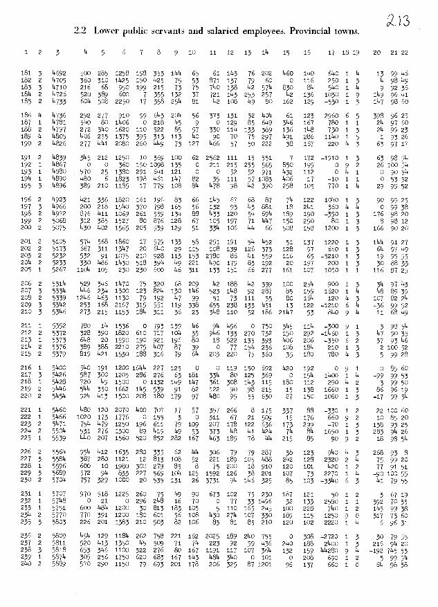
SUA%O1 JrnzrnLAOJd s(ojduiput S1u1AiS qqnd JMOj

ç 96990I099L4T96TO1L9z490z9L1TOz4696Lo4io6oL6699Çotzc664zi0699O0TOI0Ottj9tj61 L91499 O9 04L194o4tL94T64z

4cL z61-6oi1i1641zci994LoILIT1611L91099)2zz400119ti44499T4494oz t69T4T00hz9910*94964z64zzt1LIL44o44r4ItoITzL4zcc 6Lo44ozLz-gocoLotz691zozZ91izz94Lz9z6z6094z94z

14 969TozzzoTO1OIz4918499019404OT494IIOz9?24094c44z09 4LLi06o6469i044LOIt1Lz04990194109091 OOTi640LL0LL4zh1Çz9466ctziotjL0014i1z691011440169161906oozil9ji009I4L4T44z66 OLz64TT094z661z496t11 46LLoOL91996zoizo9L4Tz4z61 L94z104TTL9Io4z4Lzol4L9o66t14Lo9zczzI916oL6L0L4T

64 6Li490t4440149czc9111t1614L49141646oz00016z4L4LloL4zo4z44 001 06-11ToL?24LLOT10949z1z6414z1101694L?4496zL469944614LLzI 09TOTozi01691ooz4L9496)20040961010099644izzoz 666Lizozcz9z1z'1z99t1coi691Izzz4901419TIzIT09zL8499644Lzz94699490964z184L9z6L6L904z9644O94491I9946194zzz

94 9691z60669dz9t19L491499L9I zz z4goz40941LozotTsj6444T4zz91669z4T0491999L99 19994L4446t6196900419Lzi44t1OÇÇzzzcz 469414iOL-66zciT949z1 9L1Loz6o16L119961o4zT6L96L1L94z4zzoz 49orz60999L141604TL911404441o9LLI4L1OzOT9916109 001 zzzio4489L444LI999L64LdLIL0L001oLozozl09909141Tzz

96 66LI-4T0901o4TLz0494446ot1L66LI091900041411iz69494zozz61 96994T09919414iciz9606zzl916646491Z991044iffiÇ9994z6Iz04 664zo6zzii091411491904194L91691z411 0004169ozLgztiçT9I44 6666-1100911410694dzl09944191499Lz994ozI004L949z944 Lz 09 49oT6oz61oz9z69041611oocziLzz9191 OOzT16109400941iz

gz 66449o9L091440944Lozzcoz96L9149910441 T9 6196L44z41zzc ooi z4Toiz98180194z941LLo64L9L094Lzolzz8846849L44z9T946L4z9044-90z909464441zz491099611z60610641oz9994L44T4Tz44 o6L9410991-z6z041z4LoLz44199644ioiLTL019 0910648z4zL44zzzi96Ç16004-911494o6LO949i69964146L094419109Lz644Tliz6999TTti609846L9Iz991z4oTT9944z94114181441141z4Lz914g4z4 6694-t19oizi-zzl4114944194z449944611144414L91z89144zz94446oz9z Z9LOT4ozi1910944TIT4Li466L6i6L041T49191T664oz64 69t1T 09T6i49L69*IIz4991041i8 czI0041*49lÇ4ÇLoz4i L641oo611COTz8T6oe9oÇLoLT914 6dTc90

L99111T0401Loi191LL99TTTTc99009o4o40I1011L96Tcc04T00L6To?61486LTo6*Tz6*16681Ç049199044Ç44

46614T0T991T619909LÇÇT611 96 oz ÇLoT16z44zczz4oz69 L694T099L6gzl4L4 9T 6I 8014116z0t9oLt1411T4L99LTæzLz i6 ITiozIL414idT6T14z9444T6LdLI09T994*LdoToz

O06991Ioozi8T9099I901i4416T 644oz4941zoo4t6Lo4ooi 964o4OTLti1TLL610IL98T 9L908)2dT94z149904z66T

o69L14ToÇ4-06168T969tozi4Ç*9t4T969oTTTt9L9zL6t1z96184 660t9 O9TI9118996ÇI9449T96LoLcO1ÇT91zooz9961çL61z 6606TotoiTtjLL99L94tT9949961T91O?T944T1iÇ?61961

z4 666z910LL4oT8z0646t80T6LLLiÇ9TToTz69694461zÇÇoT101-Li909Ç9OT LITTd6L199961 4gI9099o6Tt6i9c 060T90zITÇtTL6zooTTT9916zo9ÇT4oL4099*I461t4 oo9z6o661o8494cd4TTO4T 8601 o6T09ÇooL98ti1869410T61LTL144dl1119z9OOT69401o4Ii464z161

LI L6Ç.ÇioL9194zoL499*LzTL6909Z090?T91LL99o6T9Ç6II0f11198169L6zLOLo6096h41464LÇi90*O9i6r4z 66ici oL17I941684cci111 ocL44æc 0110z91094zLzL6Lt1o9L61zTTOLL9I9f14619486z106Izo90t1109O9T8L12.81z 96964Ç

9096e6119tO9z41614L49t1O41966016LLzz69LI981

096L91cTo4-6z1z91o6iI9Ç4LIozt0944L9zgIï 966t11610601941zL6cdctT TLL44IÇ46L00964 ozÇ9zLt198T

946611Totgo49Lzi9T oLLL66T o6991o1L*4c6i 86lÇI09110096LLT 1L9c4L1 OT 4tT 0T09oL1zBT9* 664191019091091æz 9L4tiT1991TlT44861 94I6900469ti19T

zzoz6i 9TLI91TtT411TT016L9T

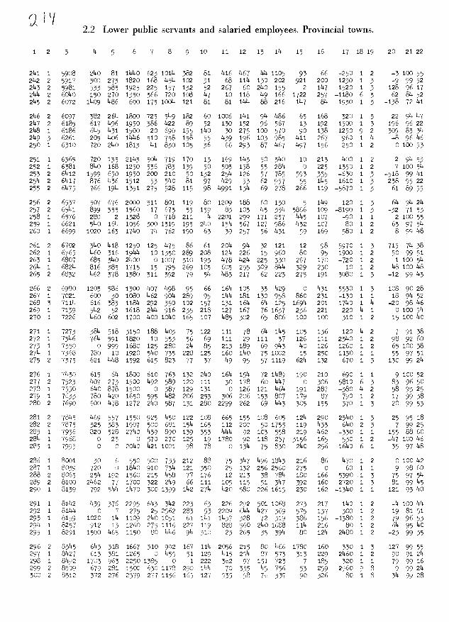
SUMOT IIfl!A01d (o1dm p.Iq1s pull STLIIIAJW Dqqnd iMO

9T 66 96 c9 T 09 9T4 06 666 L 6 446 )2T 691 94T1 LLT 6L6T 9kT TLL T169 T 006 66 6 9 6 0961 661 64 94L 4h 464 oL 991 COT 9kTT 049 0061 190 6L9 6069 T 661

91 66 6k T T 0T6 491 k 61k ILT 66 T96 TTT I O 494T OLTT 696 LCLT T699 I 96T 91 T6 06 T T 0991 6TT 416 464 L9 96E ÇIt 611 14 649 0 4911 196 419 LT99 T L6T 44 66 LTT L T 066 091 O9LT 99t7 09 LIT 9401 t1IT L91 T66 014 k991 914 4t19 4949 T 961

46 66 41- T T 0991 911 09 966 44 691 61 014 96 999 09 0411 499 004T 1619 T 46T o+ 46 t19 T T 09 911 91T 9991 091 094 9l9 611 LTT 911T LLT 0911 4C TT6 L419 T 961 64 96 6L T 1 0941- 94T 996 614 1k 914 k6t11 T9T 19 1401 090 60TT 91 0101 64T9 T 46T 14 19 61 T T 004 LLI 4L4 696 LT9 9-99 COlT 44 491 T91T 61 4kT L O 6918 T T6T

99 001 1j T 1 091 LIT 6)2 9901 104 111 9T1 69 6TT 196 699 4611 9L6 669 T918 1 161

09 46 ITT T I 0t161 191 041 LI9T 9TT 084 019 9LT 191 6661 004 oL9I 994 T6L 66T9 T 061 4966 T9 6 1 olLl 091 164 L96 14 ÇTT LOT ITT 99 691 116 O0LT LL T9hiT 0019 T 681

94 L6 4L 6 1 0664 991 090 99L 94 901 TT 9LT Lk 949 LIT 094T T6T 941 4909 T 991 0996 6 T 1 09 0 4LT 0941 941 141 41 044 Th 946 0T6 0991 0 01k 6609 T L9T

190010 T I oL9 99 911 6991 969 k94 6k 99 TTT 46L 004 044 9 cL 1009 T 981

9 L6 44 1 9 0991 941 091 049 6k 1161 0 9k 96 1001 119 0901 0 0 666k T 491 99001 L9- T T 044 491 9414 L41 911 16 o9LT 6T LTT okT ok4 0 61 0 996k T 991

09 88 44T 1 1 046- 199 611 844 601 16 999 444 64T 068 649 09k1 814 019 946L T 491 4166 k 4 T 099 649 6TT 44kT 04 OOT TIT 491 941 189 004 ko6T 494 414 4k9L T 191

9T 46 41 6 I 0941 061 911 609 90T 441 499 901 TTT 049 416 0441 L44 699 499k T T9T

64 66 Ol 6 T oL6 441 404 699 69 191 66T1 091 141 L94 091 TklT 9L9 009 069k T 091 96 66 kl T I 06k k8 6ki ko9 441 90T 904 641 901 189 464 0491 019 09k 669k T 661

4h46 94 T 9 094- L9T 161 999 IlT 9TT 0 141 611 L96 O 0041 8L9 099 044k T 8kT 04 96 49 4 9 0194 906 0 L99 09 9kI 06 TIT OTT 694 169 0090 4LT ko9 614k T kkT

14001 6 1 I 069 OIT o6T 6991 1k 94T 99T OIIT T41 69L 019 0091 99 909 049k T 9LT

9h 66 061 4 1 oL9 161 919 6TIT L4 46 69 kL kL 6T9 419 1641 899 119 4L6k T 42.1 14 k6 44 1 1 0411 041 4T TOOT 6k O9T 091 41T 811 46k 094 0T6T Ol 09k 996k T 9kT 94 OOT 49 T I 091T 911 09 496 69 681 411 48 9T 091 4TT 0991 666 0 oL4L I 4kT 09 T6 86 T T 0961 ITT 9TT kL IlT 6T lIT 69 94 644 OT 0191 164 99L 996k T TkT 84 16 k T 9 OTT 961 401 491 99 9k III 111 6k 609 991 0416 914 996 6)2k T IkT

09 001 41 T 1 016 001 001 909 49 106 499 LOT 49T 0901 009 ookl 109 099 9TTk I okT 940010 I 9 OTT ITT 961 kÇ9I 9k k91 LTT 811 441 916 t9T 9T9T 14 T94 64Tk T 691

9986 OT 9 1 O9LI TOT 9691 901 99 991 T6T L4l TOI 044 T6T 9011 696 9T9 9ITk 4 99T T4 96 91 1 1 06T 16h 099 946 061 191 991 46 691 906 T99 0901 06 009 TTOL I L9T

9T06 901 6 T 0644 149 0 619 66 401 991 99 46 969 ko9 0041 994 LOTI 0869 T 991

4966 TT- 4 1 0904 161 LkT 411 19 kTT 699 94 6k T64 114 0961 9k4 T99 T699 T 491 89001 89 T T OT 06T 6T6 998 604 490 409 401 69T 66k 41 LILT 496 919 9199 1 991

94 001 1 T T OTk oLI k9T 046 4Tl 909 9k9 66T 016 kool 0 0091 094 499 ko99 1 491 14 66 04 T 1 0061 46 09 096 41 9TT 9T1 801 69T 044101 9961 914 099 49L9 T 191 94 9k 4TL 6 1 ok64 96 TT ITT T6 96 90T T9 99 4k9 4TT 04T1 9Ttj 096 TOk9 T T9T

9 66 9 T 1 094 69T 64 149 94 L4T 66 69 061 19k 9k o9kT 691 0101 6699 1 O9T 94 k6 69 T T 09 kol 169 996 kTT k94 941 09T 461 6141 006 9401 991 094 IT99 T 641 44 001 T T T 06- koT 4 k4T IkI 661 IOTT 9 lIT 91k 0 8T4T T 091 9L49 I 94T 64 Tk 16- 4 1 0619- 601 9994 944 49 LOT 49 64i 44 6k9 kl 0941 444 669 1949 T k4T 9T 16 99 6 T 011 691 4 061 09 991 6011 09 6TT 109 114 0001 9k9 ko4 k449 T 941

44 69 19 6 1 o)24- 6TT 99T 9kT 69 961 1669 96 4TT 9T4 LkT 1441 96T 99L 4k99 T 44T TT 46 94T 6 1 OT9T 4iT 44 k46 19 64 619 L6 19 094 44 TILl 949 9k9 k199 T 94T

1966 9T4 6 T 069- 446 664 48k kL 9TT 941 161 04 OIT OOT 0461 049 6641 TT99 T 441 94001 k T 1 0441 411 0 99T 44 941 404 04 64T 49L 964 o4TI 991 099 1969 T 141

44 96 T T 1 009 LIT OT 096 04 69T 691 6T okT 61k 904 69TT 461 01k 4969 1 141

64 0010 T I O4T 94T k69 k99 k9 46T 99 96 4oT 049 19 6191 091 OTk 0149 I 041 9996 9- 9 1 096 k9T 119 496 601 961 669 44 941 96k 0T4 9991 909 4oT T9T9 4 6iT

96 69 604 T 6 04TT 941 06 ok4 OOT 4LT 04 091 441 069 OT 0041 149 499 9919 1 990 TT 96 96T 4 T OO4T 161 61 k94 96 141 041 14 69 119 994 o46T 969 k19 4919 T LtT k9 96 TT 4 1 014 99T 49 989 96 111 9001 09 191 694 41k 0091 991 T96 k609 T 991

19 1k 941- 4 1 0661 i9 kiT 911 99 991 19 T9 ITT 9001 4kI 009 999 6ot Tk09 T 491 14 98 19 6 9 0811- k4T TTLI 991 69 811 Ol k9 901 OTL 994 0441 okT 041 0909 T 9I1T kl 96 911 4 T 0141 k9l T 441 091 09 L9T TL 141 k4I 4TT 4T6I 494 664 1964 T 49T T4 66 6- 4 1 0411 001 116 TOT 04T 911 99 14 TOI 949 991 OT9T 6kT coL LT64 T 191 44 001 6- T T 041- 99 66 40T1 r'1 k99 919 19 194 11101 619 0991 19 091 9064 1 19T

TT IT OT 61 91 LI 91 41 91 41 TI Il 01 6 9 L 9 4 9 4 T I

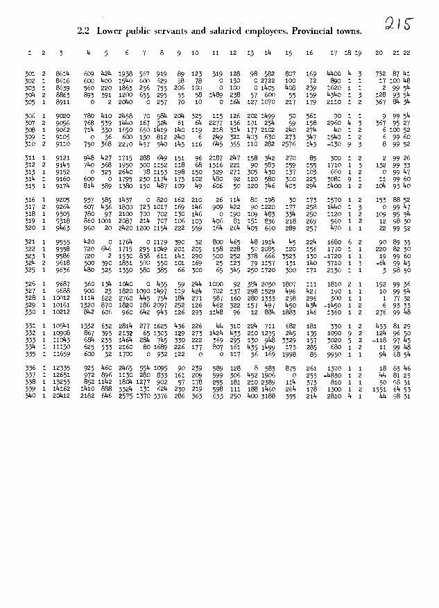
i4 96lfTij0193I1T34449914 00110434494949939L44 0L4T 4L42911928T3lTIjOII01j444 11914413T00419LT119309111 99TITT964612043119141tilÇ4899OT11T291111T64414 96o4TToig4L4tITI6943 0131914439LTL4106LL2T 11091211T1 3494424TT94443 19ii3T0491r4410906T 21 90466460119144908204119691L614921TL44911 49911ioLd1914L9494993T69464206460T 1i44491130911426444211944

114 99116TT046649966169194LITOOlIT3460GOLT240096491TT444911 66TTZT099493dLi66111 441191Lo9LLT9236991 0809T2446429O4TTTTi4Ç411 L6811-40304L4T63448116041463694332odd411L1193119111443I99dtjOTTT44404 96113136o6oi44141134431 013ddtI1131114LI6314O4T 49I4TI464L9890601Tcc63 1931odd191399TIL1123old11119339d11429T LLI111823493441Tt40T1Idd

911 669L331094191114991119931969111146393T41163119096909311911101TOdd44 4693T04111-0411L61L4I334911921343L6o3 9910291oL90341T9TOTT643d LLITT004961963dddl 091091L94TLI191114L11109L333911TTTlIcolî934t14 6601IT061L31196116361 963LdT bL1131f611L6111 0601 0391dl0069996TLzd94 66341T30191TITLo910403 10436000T1111364d1O0t10T1141094L996T934

04 964I10413ILT004OZLI 0431d4900499494094O4dT41409119496T434411 66194TOIL40111IdiL411 6LdlT43691TOT04400414910640069196313d09 66611IolLI-04143449999L414100406111111199d904413olL9946T434cd 19011TTOLLT9410114803 o493394T4031036tfOT 4634TLT9119OIL9446T3344d 690639099111331111161 9149110093do6d6LTT O119LT003114446T134

34 66lTToLlL436930994011119111916443321411 0031 0312030964916TOldod 9631T094693913949I4T199011401901L0L11T1L901TOOT 0999146T614114466013T0311043lddd816oT0610911041bL ooL0013L6o9L4od6T914L116604T0t111T943LLTOZZT 063316069111691LI0T dlL009T9d1L09119363LTd34 9944TzTOL4T4LI0496109III93013391029 0L411T494Ld64036T914

01 6611013I001111163401191L031o490961160iL91104109d169411T911LT6T41409 66TTT6090443300409403136OloT4LT11LTT 04346LT00090916T111dL11 66031099401LdI041404ILl63404196Td411 9L0119343403416T41444 66bdTÇTOTLT44164148406T339T4T899113411 004o46T994011L41T6ZlTd93 6633Tood49oL941LiZL9TI9614161199934TLTL211613T6T1T4

34 66946041-4119L43393OTT44411991T41110114L411OL2Z994o4LoTT63014096693101141LldÇLI0494011TZd61139013319OdT0099dO4oT6160424 GOT 93T0111L201133012 LLTlTd9T361101161111 04904914dilL3906T90dLb 46L94d1109639416411l161941LL33119T9IldL9T01111164499L94063Lod114 666TT06T940466111 3039314T14241101194OL911l011109L0306T904

ii9 L9d3101136LTLIZOLOTLZT119TOOTOLL43 001101301169T404114 d6931dT01141164144009L48db6911194444634490021T6d4694999ZtIOd11663TT029164390114011 0001000190344L943d99T0330946499Tdod911 GOT LITT0692L0012ZL3 0CdTO8L946390090114100110099198T304111L9I4Ldi001111691Lo939496831614dlI696T6L94946111311609111983lOd

23 120261 91LI9141111dT21TT0168L961143T

-s1SUM0TpuiAoJd(o1dui puiqstflZ STU1ZAJS Jjqnd .IMo'[ gg

2.3 Skilled workers. Provincial towns.

1 2 3 14 5 6 7 8 9 10 11 12 13 114 15 16 17 18 19 20 21 22

i 14 1639 267 1714 6 139 82 37 211. 15 11.3 23 22 10 86 170 3 5 Z4 7 1442 14 1650 331 1142 715 101 77 19 35 0 17 114 314 loi 111 20860 2 5 7 81363 7 17314 99 192 780 6 217 145 149 27 148 26 12 17 87 600 i 7 -7 79 14314 5 1819 113 122 780 57 121 39 25 71 141 11.5 52 17 105 550 1 6 10 9914145 6 18914 232 118 589 0 2147 82 29 306 68 15 79 26 105 11420 11. 7 35 91 45

6 6 1911 118 139 832 252 72 35 142 15 65 29 65 14 30 2140 3 7 0 98 607 5 1911 86 1614 7514 106 101 38 28 181 51 0 102 5 160 7140 1 6 -14 98 1448 6 1967 101 183 833 58 1433 101 148 123 90 38 101 17 135 200 1 7 0 61 1469 6 1985 306 86 910 149 80 63 314 15 25 16 29 339 93 -50 9 8 -161 86 36

10 5 2038 173 110 767 133 120 144 28 83 149 30 105 147 1140 290 1 6 -3 99 141

11 5 20147 232 268 872 140 108 140 149 23 13 25 88 14 139 850 1 6 iZ4 91 3512520914 2631140686526014333166606799 13 97 14io14o 39145213 5 21114 116 161 816 112 1114 50 28 33 Z4 21 120 38 117 10140 1 6 22 914146114 14 21148 2914 222 910 10 95 614 145 11 140 11 35 30 152 260 6 5 21 98 14915 5 2160 182 226 705 200 173 51 26 31 57 26 314 208 92 360 14 6 9 911. 147

16 14 2167 100 1914 625 300 139 29 50 129 61 51 252 0 156 160 1 5 2 96 5117 11. 2172 814 161 562 25 75 27 63 62 511. 27 210 229 123 1470 1 5 5 98 5218 14 2180 211-8 1814 780 159 152 95 66 8 35 7 7 19 128 730 1 5 -32 96 143193 2218 321433352720028179111 281152897 12 22 099 01415120 14 2220 172 79 997 318 207 36 142 10 57 26 13 6 228 300 9 5 0 69 60

21 14 2290 367 2145 780 86 217 58 39 61 83 27 614 15 i114 -1410 1 5 61 98 14322 14 23514 327 1214 910 132 149 214 614 61 105 58 81 23 iZ4 820 14 5 -160 9514523142363 22618890010512239146 83735146 731149101015 9095145214 14 2367 150 199 935 3014 67 30 140 35 147 73 83 25 153 350 14 5 -7 9114625 5 214514 202 181 8214 16 195 51 144 153 147 57 52 15 911. 1590 1 6 ._144 96 146

26 14 21473 362 309 975 23 85 32 28 119 87 149 77 23 1145 770 1 5 -188 96 50271421481 190151750107351471456165852142314 514 145 -9015 8985228 14 214814 159 226 9142 92 320 614 53 77 92 26 1314 32 1141 180 1 5 3 99 14i29 6 21486 3142 157 603 167 193 59 35 171 103 141 614 714 106 370 1 7 139 95 31430 14 25214 267 172 8Z4 0 181 73 33 31 83 9 129 170 196 1880 6 5 153 9835

31 14 2525 195 2014 600 181 162 28 37 1465 146 37 119 9 132 1470 1 5 -21 9851432 3 2535 140 2149 710 137 165 69 75 148 126 143 252 0 173 1260 1 14 118 99 6033 14 25142 301 238 997 1114 178 78 55 538 81 14i 71 190 i14 -2260 3 5 99 98 149311. 11. 2556 1149 158 10140 130 2142 56 50 39 59 27 122 90 1214 390 3 5 0 89 14935 3 2596 259 168 1010 223 263 77 1149 23 137 51 1145 33 139 180 1 14 0 66 36

36 14 2639 269 230 101414 814 236 85 23 1.45 36 149 1145 29 132 1100 1 5 66 91431437 5 2703 250 173 9149 270 282 87 147 68 78 75 70 12 96 380 1 6 10 914 14138 3 2783 182 2614 1020 88 206 83 140 96 56 37 136 30 203 1410 14 14 -19 99 1439 3 2801 328 190 965 170 129 142 142 108 146 311. 93 52 223 1100 14 14 11.14 98 148140 3 2860 1432 282 997 123 198 38 53 2014 117 145 152 125 150 0 1 14 -21 79 60

141 2 2872 2140 103 780 32 116 144 19 351 145 21 221 232 255 1010 14 3 93 8 26142 14 2877 337 187 101+0 628 1114 31 29 150 146 147 3614 7 129 _15140 9 0 37 81 19143 14 2899 126 222 975 318 1149 140 14 115 103 32 250 67 109 1420 1 5 0 99 514144 2 2921 5144 350 558 1145 1497 68 195 298 61 146 12 312 158 110 3 3 99 36 30145 11. 2923 197 2814 910 121 280 61 16 165 514 2E 1014 32 127 1190 14 5 155 98141

146 14 2933 208 206 1097 7 115 68 25 229 62 145 1142 62 157 610 1 5 5 914 52147 2 29314 188 395 800 871 0 114 61 36 93 73 32 25 188 250 9 3 0 314 53148 3 2958 217 187 1213 158 200 148 52 111 29 61 80 113 176 1400 1 14 3 9852149 14 2990 237 3214 923 120 152 148 67 178 95 35 126 3144 186 610 1 5 147 93 14850 3 3010 3147 335 893 2140 198 146 78 133 38 31 227 6 100 -260 5 1+ 0 98 53

51 14 3061 3114 1140 935 614 2114 86 61 75 71- 14 111 573 170 550 1 5 39 96 6052 5 3061 2814 251 953 77 14s 121 32 1143 65 142 70 26 179 570 1 14 157 79 2353 3 3075 14514 362 10140 175 2142 67 149 108 69 35 1145 17 225 520 i 14 -192 99143514 7 3079 178 201 1151 175 3114 66 28 100 58 514 391 50 17C 550 9 7 -3 933355 3 31147 510 3 700 178 537 57 142 162 1146 85 3148 iL4 221 1590 6 14 -3 93 514

56 5 31149 310 2014 12214 10 266 39 70 814 52 27 1145 70 155 1160 1 0 -20 802857 3 3155 235 2143 1127 208 200 71 92 21 110 142 190 13 1614 390 1 14 3 98 3958 3 3232 323 1409 1023 222 119 1+8 56 1460 66 58 130 80 169 1410 9 14 2 975059 3 3252 202 207 101+0 115 231 98 105 356 73 60 169 14i 166 620 6 14 3 99 5360 3 3277 208 220 1267 160 302 147 614 90 116 28 140 2 171 600 1 14 14 98 53

SUMOEI PU!Aod sJ)1JoM pIIp1S

tiÇ4L?-41o6t1411911144LZT4L9ZL0946?89149L9966999014OZ'9669-tII04469Tf1014401 4L41140?14TZT919004 o4ZlL6TL14to4461114 46119?ç6 o+-91Z99166ITlffTLi91IZTILl4946141199?t194904Z911114 g64-46OTI19?ZIT940419?T T691149196lIZ4ZZITÇLt4go4ZIii09 464o141009TTZÇIII?94994999494otL91491OZ9T811116LZi1iO4Z911

4 9644T09T19?001191ZL98T1L419i6iZ444ZZ66?LLZ6Zo4LT 96491çI094?Z6Z949L4 01466644L491911OT9T99?1149661Z111144 66o11T0Zæog911LiT4444?09?19T91111109 049Li494Z69611ç4T16i 96OZ4T0011oL4).g0644).Z4T099Z94iZc 4911L94o9liL4811ZZIT4666Z419444L1LTIZ414Z46Li1?96Z640649441OLZ4949LLIt1ITT

9Z 9600141094L9ZZ411LZ19190994g004L44Z6164Z911949L11ZOTT4? 119Z9io44T864o9ZL4oçTLiZ9L4).4964Z0Ç9T9411Z4T11111ç6oi911 6901010Z46T414?oZ4i49906z4ZL9Z404ZL46491Z191491190TOlj 6ZZ99To4Z689oZ6099ZTt991LI1890ZOZIZOL44Tço4ç6414LOT66 461166otr16?ç11T816998441Z11ç911Z1998ZZ94400?99411Z901

6T9L4ç9oZ9Tç190111166984ZL99çL91cc111T11ç99L9tt1?40TL4 L6ITTT01991?9Z+îT94Z4LI141446Z114466ÇZTLIZçIZ644i411014Z 996114T0094LZ81194LT14LOT11?64Z9o6T09?4L4TZ9Z9444111Z401OZ 69i6Ç909çZ4Z41ZI?ZZT9LZLI09401Z949LT0411664Z41i6iZZOTi 66Z+j108999144LtOZI891491T649TTZL9Z6941TLZ411Z99Z114TOT

LZ L6TiTOOZ461ZZ9OZIi06L966cc414946444011199TL6T4TZI4OCT9T 06ZL4ti0144hZILT6o449LLZ94i4IL4T490Z0941 i411911Z66i4 896Z-çTOZT06?Z9ZZ).Z9ZOZ81496401i9Z14916194? oL494111Z96911 96ZI09ç691oIl40411019819i460181694LLZ94014TZLZZçIiçL6Zc 1164T-41040146?01141Z1011T96494664Z49LT1189LZZZ4Z001111196

911 66Z11T094Z9ZZ+jT01114ZZ6914Z40649ZOZ?OZOILIZ0Z469011446Z4 4641-4TOIT-911f4LZT441LoT4LZloT1141ç11ç4LZç9oT60169Z99011Z11644 19L4oIL4L916Z9199OZT6T4hLoT9TTOLZ4L6691L4TOZOI1146i4 660iTOZT191aLTTZZZI949901L99604491T96oIT44?i6644Z6011160111101144ZZ6196hZ069L110L6LZL4t1Ç4441 Loio6i4Z6416Z4 464-6 og4991664ZZT44401414Z016Z1944ZZT0110194Z91499944060946996O9L461TIllLZ49444Z4T964LLt494LT196I899L94468 9T 9409ç1oLLL4ZZTITZ4LOIT911146L491640041L44Z44Zt94Z9909 LI69-11TO4TT-9116i66Z1969441944iILTTZT1991OZZ111111944L944491?6o9T1ILZ44146ZI106Z9111109411604O6IIÇLT4LZ6ogç499911 96LI1110Z9-0419ZL064Z916Z9T969444L44096L6T0Z4oLL444904 98T-4108TZIIZlIZt1LI0441T90Z4gcL0111T9OZOI104981144L4111904 Z9ti4o601611191IT9t1Ç4449OZT9119146ZLZT8T4464ÇTZ969444944 961-fIjOZOT40Z4L1T4916ZL1664ttliÇ11?ZZZT98Z96Z0694çZ9L? 169?11T004119?94LZTZL46ITZ911Z4T4T90?4601LLZZ6ZZ994419

04 9691111oL484?41LL4i41T94Z44T4L4oi944LOT90100119944096i 9641-11904L?-181Z66L11911469Z96oT46ç094Z110110114Z66cLL9çç6161 9991TTOTOZ191094ZZI194L616T411T0011499Z6Z4oLZL9çcti4 19 1IIO9ZTO?19ZLZZI996oe4448191L940411L990T14944ILZ4 1694T04-Z618LZ116?91?6111ZZ4111101911Z0049Lo444i909449L

ZI 96IZ4109114Z16?44i96Ç11TZ4Z4i1019Z1j161994944Z9L4411414Z196L41109i1Ç4oÇ619LL49ZT4i901044Z9T0441 99Z04ZZL4ÇZ+jL9? 46o116oiT-IT?991OZT01194LTLTZL901LZOI Z4L44?6ZZ444444LZ4 4644109?iLT41111ZZ64+11I9ZT94TiTL64444i464oT11ZZ4444tZL04 96 04111O1ZT?4TZ440441494104141111491j9T4Z0IIZZ66444c4IL

9419091014T94Z4011Z9LiLOT66944LttjOOOT9I4L914410109440110IT104161141Z99461696L1190111109009116911ç16? Z4 001 ZT-101?ZIZ4L01?o444194TiTT0604Z ZT OtOIILTT91111Ç499ic 1161TT008OLT6LT46O1o?I811T9Lî4Li90T?61?996ti4iL4 666-4I0649L1641og0696L4611TL9114tiliZ4?gILT OT211ti99

911 96419OOT-LZ99114?4L441661191494?41801691ZL616611494 469LTgIoI?I999tITZIjZOTLLoiL949Z14æ 0001ZÇÇ4g?o64419189L1110?ZI9L1IL911??+j?i9Iti999104LI?ollI?11Ç9LI16IiiIO01ZL?O09801j6i189ÇÇ1g?8O1 1Z446cÇiq 964104h911OI9I199619T6LiZ6LZ01406?ÇiT9

??o61 91LI9141111T?III0169L9t4?T

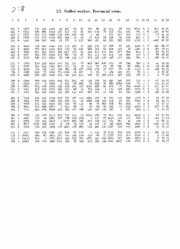
SUMOSi»iOMNIIPtS¶J

4'i o6Ç11oTLT91699641IOT OCT99T6i*LTOT 4991006006T11TiI4T14 g6OTIoÇTti14LT6L9T 6T 661O11T091 841 66 409T 019100904911164T4h 661TTOT6T919191L4LI 4Ltgo6041 9144LTL9611i1Ut?o1646oOTI14TIl194it1o6L9611o4OLIT 9LITT0961i6gt1oti014oi4TÇ10099T46IT41

06 66046T0991L4ti091L14T 111109119t16116LT641T oU1611606g4490491041ti4 6606,-4T01161tp1Ç69619661940T6T60166999044T9911664T4Ti1611ti4 6g1-1T0011114111iL4LTTlt1TL4g49T441LL4I 06611lt?T006146gT91109 L6TT-T10914L49940191 LgL4T0641g4TgLLLL9Lhi9100999091Lt144 7641Ç60911-111164ti4t1L99TlTd694TT9TL4Lti464ig91 64gLLL1911

44 666110914110049OTT19T091goe LT4i1.16996t11Ill 099494LI411T

ti4 996L14L01161g419966i4g9699IL186419019114ti1411411L1111114 66L4TT04909011ggÇ1961L94'iTT4g6041140161T04T44g4lLT41141 66414TolLl114664111619110149TIT9196649141L91TL4TIlL1111114 L601611064-9410414110441T1991101LiTogL8011ITLT111911111TL1TIT

14 4616-4T09411141911196611T11101104TLti4914L1TTotiti06gUtioU1011144 06CT410LUL0914gT4L1o6019U4lI91044191004T411LT4TOOL164TLti L6LTT41ogti4-614LL4L99g811T904UtiI4gT9490440011tiLti4ti41999194114 i661-1T0190f191T1Lg44446141OIl4gT4'i001910O'i41199TL4141 6611T4TOTLLll011Ud1994116T96441TL9919O16TT4100401491941

14 LLo46oL46g4L14400, 4tiîTg994Tal41T6g49L10041641co49119144T09 660TT094L1419994o4gO00199400T o4L01914401199091ti444 6614-010441oLiL4LL9164LT961TLIl1941141L4Llg9041L96Tg4444T91996101 01069i1444g41IL9411L4494L1 01101014614tg4L4414T14 666-410149449t16L1L4tiL1416f1LLOTT6440910191194044olL41T4T

09 4690T4TotiL994LOT999tOT4114L1LoIlOT9449L06919944441TL4104T9196119410949114469114lOT104L914Lt44109411L4T9Lt44161144 96li4To4'i6111111194001Lol491969LTL9o1 9614L11T61OL1611141911Il L66gT160I4Tg49TT11118144TII111g664910166411111444911144L1TLl 19T91410941014L9991L444T4946411T4L464101101L1i1999OT141911

L4 L9L11I-4TOOLT9114g401441411'o'iLIIOLLL16906661 bL0644141T0416L4T001941141449g6T4LI06CL911 69 l4O4461L441'ilT69L)T10L944L6TL9TL910Ç9LiT0116OOoe4LooLd6T41T6i 66 9T-i1C9L49TTL4LlL6010461816L1L111411T4ti11166oÇ111Il 911IOTL1194T9Ç4TTodrt01414119Lo419010196T 0l1161T1T

11 TlOl6191It9T4TfITdT1TTTCT68L96111T

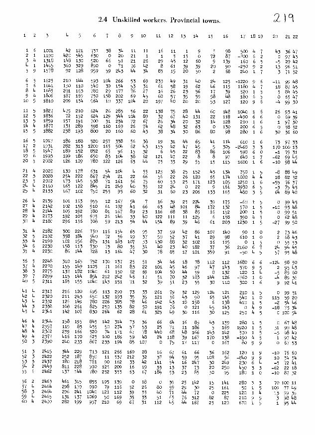
2120 21 22

53 36 470 97 53

-5 29 4213 96 51

3 71 32

11 9914818 87 145

5 85 1450 65 147

- 9930

26 93 Si0 69 391 97 3005852

30 36 60

739733170 100 13-1 79 31

-62 99 145-10 98 144

-8 88 5918 82 52

-55 76 37-3 75 14561489140

0 99 145-10 9358

0 99 51062148

-2799502 731462 68 5305553

25 944 45

5795148

-1214 98 502 95143

-5 85 60-48936

9 92 141

0 99 51115 59 20-2 514 56

-18 75 3140100514

0 67 5831 90 58-3 98 59

1 97 5206753

-10 76 60103555-5 72 51

-622218-10873270 100 11

109 77 5139935

3 98 58195145

31 14 2182 300 226 750 116 1514 65 95 37 59 52 86 107 1140 90 1 032 5 2192 358 1814 5l40 72 56 19 37 50 52 37 Si 29 98 610 1 033142199 102156875131183107331308832102 16115 015344 6 2230 158 113 730 73 80 35 31 So 23 140 182 37 36 2160 6 735142230 86114472813161414730 788517101359 91 -504536 5 2258 310 165 752 170 137 25 51 314 56 18 78 112 112 1680 6 637 14 2270 155 1149 1105 71 161 83 22 101 55 56 97 57 1143 570 9 538 3 2275 137 182 1050 61 150 62 69 1014 50 144 59 0 132 120 1 14397 2299 1151144 854212214214617 517032103 1144 126 -76010So 5 2311 185 155 10140 1143 151 71 32 39 51 23 55 30 110 300 1 6

51 14 2317 216 120 695 113 299 73 33 261 79 32 129 1214 121 210 1 552 14 2320 211 2t43 650 132 193 35 35 121 56 53 90 65 1145 5140 1 053 14 2332 126 1149 780 226 385 78 56 1142 43 10 158 6 138 1410 1 5144 3 2338 108 261 825 250 135 82 50 191 76 0 121 55 1143 0 14 955 14 23141 1142 107 830 2614 62 28 61 325 59 30 116 30 125 250 14 5

56 14 231i4 158 195 8145 1142 3114 73 36 66 65 16 85 53 139 280 1 557 4 2357 119 83 1455 50 2714 57 53 25 71 11 186 5 169 1920 1 558 14 2362 239 166 520 714 171 67 78 145o 68 58 166 1143 1142 570 1 559 14 2377 1416 170 625 100 186 59 58 214 118 39 167 170 138 -190 14 5503 2390 2140233 867233195 85107 07517117 0167 809951 3 2515 31411. 229 713 121 266 169 28 16 67 61 66 36 162 120 1 9523 21422 2521878501153721232 379145995108 56-8409953 3 2537 180 218 781 90 162 33 52 114i 514 16 2147 30 2149 230 6 14

514221449 8112289101252091619 33133773 20250 55033556 21462 1371547802523536367185532385 50 95 1801056 2 2563 1461 315 855 195 139 0 18 0 39 25 1142 15 1141 280 3 357 14 24465 298 179 910 79 116 52 26 80 59 29 30 25 161 50 1 55832465 29624110501211123935 50715472 0225 1201559 4 2565 131 137 1069 50 169 35 33 51 65 76 312 82 87 210 9 56042570 2821999372106967311125554167 25120 67015

2.4 Unskilled workers. Provincial towns.

1 2 3 14 5 6 7 8 9 10 11 12 13 114 15 16 17 18 19

1 6 1001 142 121. 737 38 34 11 11 16 11 1 9 5 98 500 14 72 1 1.190 1420 5145 630 0 20 21 1 1 5 1.5 0 72 87 -700 6 23 14 1318 1.48 130 520 66 51 21 26 29 145 12 60 9 139 160 6 514 i 11465 360 329 890 0 71 76 52 8 61 39 39 20 90 -250 9 25 9 1578 92 128 959 59 2143 1414 314 85 15 20 50 2 68 2140 1 7

651625 2101545931014266536923314931 140 214 125-1220967 6 16141 130 110 s5o 39 1514 53 31 61 58 19 62 56 115 1180 14 78 14 1685 201 163 780 29 177 76 27 16 26 23 56 17 39 520 1 59 14 1806 187 169 750 158 202 69 145 60 57 35 59 58 148 180 6 5105 1810 2091314 9614 103371014 20 197 50 20 20 53 127 12096

11 5 1827 475 210 6214 26 283 56 22 138 75 28 144 6o 1148 ioSo 1 612 5 1836 72 152 6214 129 31i4 ioS 89 32 67 140 131 22 118 _t490 6 613 5 1859 157 191 700 31 2314 72 67 26 314 20 32 114 128 210 1 611414 1877 1.312895981.601692675 621483263 0130 2006515 5 1882 238 193 800 20 160 60 143 38 314 30 86 80 98 280 1 6

165 1917 1861885202573385638 1931 444 65 4i ilS 6101617 2 1931 282 313 1200 165 5014 62 53 155 52 147 55 5 305 -2560 3 318 5 1957 189 152 852 65 96 15 32 6 45 22 83 86 106 590 6 019 6 1993 199 186 650 83 iO4 38 62 121 147 22 8 8 97 6140 1 720 5 2002 126 109 780 122 126 63 144 75 33 29 55 15 115 1600 1 6

21 14 2020 130 178 631 514 1014 14 55 123 38 25 152 143 1314 750 1 522 3 2028 2514 222 867 2514 21 22 66 56 22 26 120 65 1714 1000 14 14

23 5 2072 173 1145 538 71 161 56 75 6o 53 25 171 123 105 1250 1 624 14 2110 165 122 8145 21 2149 14 35 12 25 0 22 9 161 3930 6 525142133 167102750255956032 316023206133165 14803526 14 2139 101 163 955 12 167 544 7 16 39 25 2214 39 175 -60 1. 527 14 21142 102 158 910 61 192 141 66 63 58 101 85 172 132 570 1 528 14 21145 105 192 780 81 167 89 23 116 68 38 85 16 152 200 1 529142173 1921059752611463314012211111125 6158 39014530142180 2961567085921351414415148939146 61203123015

66041910661914011401 t19OLLL93649914LL9964T49964 oi83 9L 6r6T0LT3-4L391oT 64L64499r6096 o69T9439963611636iLI 001 4-36o64OTOT44T9014811664h091943093100110449394181191 4949t1ioL6660T9644466L9L9TOT964901L96643 4i39Ç4ÇL

44 96 0999OLTT403901031990934TOL6499t134090TL34L4t1TLÇÇ4911

64 66991otiL06164L033119999149964Lti34TT9OT103L0399666

LT648TT6109649OT994409694943LTT9T090TIr93O4TT694431111LI 960310919TT461433L99919441400341T49 0694444161161 1901-99oL64914T9334349493Lti311LO300969064c693443T1

94 96Ttibti44433TooeLti4T199TL6966T4L9T4401409394344111

96 001 066o643316oToo6643TT 003 43044 o4L04343OTT

c3 469ÇT03L-496994t*0464ti1itILI9ÇTO46T4o6490Ç360104 36L4tiOtiTTÇ9TL64T4Lt1Ç464TTt1901494990164T339T4614ti90T39 9913090143139LILT4916TOTL340139114LT 666330439cjÇtiLOT

4 99L410399414636L6094L3o996649T3190614L34914ti901

6iotj6OLTtuT61149T8909L663969Lti9113I0T60366TL3146401

99 969ti 9L4TOCT9114499666L663963003T4433431L04tOT311 66t-4603986T46913999t6Ç99946T344139TT99T96T9904Ii4OT

6ool ctT09194T963L639TtiTI9696634091090196T963oçocÇlOT

99 09-4110939193T196L911T3T43T39994461969961OLT9T049TOT

4 3L9T6o9TT634L6TOT6LT34T919LT0440444L94T30T3110630014901O9044931OTT941T64L611L4T946T990001991L33646e666

L4 LL9T9909316LTOL9Ç4Ç469LT94098IIT8TT03016034LTT6634960996319406490311L44ti06LI8994411 L9T090T333644L3634L649LOOT091991464494660916tiççL9143T093T603603L363996

34 969T11c009-L43494441931319114413463OI1OT461T039262Ç4604 L66t6080191T969T993999611449T39913L99T43T3363644 96oTt94109T3LT4L4TITT03TT034ILTT066619633T63446

49 4-66o44-16144993T469T6649409963L9030194T46116343684 16c4i013-3919016oTL8949L99949443T4L4T603o4TT693ti16

64 199TOTOL3TOLT4960939091996t063ti33tiIITI941161999340643 1146 9339009-981193OL6t3TT9LLT9T006019L40096993T699T 3L49oToT363199ILT398999394131696969666111931669311999663T-4T0113199T441L4T430934994tt06T6L49003993LT939L9

06 963311T0LL6LT931699TL4091039344TL9T49LLo36969093499

499OL96091069030LT69L4LL460169600962T6416LL3449046699109L6363T4993TT4T6LT639114TT99T3L94916033LL36996646 o4T096-441L999TLT949T9666949616901ILT93T99L3ti4909 36303-9T0046046933T34999306L9o4136696919T249L343893 TL3-6T0491639L434694194L69344TL3TT36394TT4L3419

64 COT 09I0191099L44L91094L469L63L9981100144L34094L941090911T4TT399049403838çLIT4LLL3T0330663L3116L

69 969t-40466LT39041136946Tt149TIT4010499439L49TL3119L3966 04TOT99T94o6T3ç9TT964L9943041946932ILT969311LL

L9 36634T09900199OLTo49L4L411994T40410043331996993119L

29 91133-LTOTOT401949196499L393L494TLOT0T64914oi699394L

4914 0460949339940994LIT99930948004193339239933tiL44 66444T oo49LT4346940946139944T393TLL4T4T3L49311

09 09444TOOtr431L4494936961944i494T4L49L461934349393L

094693TOLÇL444r9449LT990034T39TTT0991004393TIL

L4 96 99tiT091-69TLT99419941LL39OL0T34L109L4436934093ÇOL

39 OOT TtI04T44939991449943L4996T44TL999430933643469496L-49o43319L8LT4499LOT64T463tioTT449TT39T30943t19994L6039003-9LT43 03630360334 09T64L034TT0O4L43TL9049604I0LT903LL4TT99L464ç689943994406 69TTIT9i9909 9669T-9i09114T40419469166g60T6T09399T 9931I69

6 L61IO9tj991OT911Li1ÇÇ89T4L98TTOTT L9TTTo449944 L9oÇt1OL99Ç9TOT911t1u19I0966TOTOT8966lç9

46TÇ609T90T4%94IL91499969T36TOtOT99T9tjT96tj393949 969LT60996TT3TOL941hT61tillT8T40309L961999919

Tgoe6T 9TLT9141tiTTTTT0169L94t4T

SUMOE1PU!A0Jd sJaIJoM PIIPN'11 I?Q :' f

S11MO jiI»JLAOJJ1J0M pjjDjSUfl

cIoIL9TtjTÇ96ç66Li8TT111111T9OT TOT0l0Ç08TÇ6OITT9906Çi1ÇOCT9TL69Lçci1OT TIIÇ96Ç9Ç6LTTij0i119ÇOTTTLT69O6iyt000TOO9LcI8LT

6oeij-i9OTTc96T0011oooo6069tOTLLTiooc1LL1191LT11I1jILT1j9L9T11t196119ij10111Ç9L1

6o611t1Oi1TTÇ11gÇL9116ÇIÇTooTÇÇT69Ço99o1TLTcîoco6o6c11 LoTL9996o6c88T h1T901goTct1LTÇTo6-0ThTL19T91jTLT6L99hOTILTÇLÇ l9+1Ç611LIÇioÇoÇ-69LITLi1c6cT91 69I OIT90TL9OOT1j1T6coÇ6hiLT

011oÇ0111cLI oT O09669OT6T OLTT00611611iILT

liTOT9TOZIIZZ169cT999ccTTIIÇLZILZTTZ9ZLZI8L9t1cOLT

Ç9o8Lt11101ZL1c6LTc9ZoT1Zli9liçO9cT11occç6691111oilÇ9TZ9ÇL9011Çl L6o119L6coc89LZTT0111Z1j91lÇ99111ToÇ9T-9I89TL9991li1996898T11IZT9Ç11LÇL91ÇT0ocÇc6TcÇ9T8cZcLLL911ZooToZL9hZ991

ÇToZT- 6IcoeZ699T1ZTcolTLÇZIioLÇ6T69OZZT611Z9T

11T09188190111116LoTLt9TÇI1 o91 T9Z Li811Ç119T

11TOT8TL6ZioZo8TTTLT01j9c1Zo6 o9000To6Zli8liÇ9ThoZI99cL0TZL96li6699119 Z0To8oZOZÇO11ZZ9T

116OT9ZoZLoT09OLli116ZLZTT6ÇZIL8T 9TZ11011TO1119T

ÇIoTTL9Z.Z9Z89961198c119T6T000TÇTli91ZL8ZO9T1oZZ116ZOTZ199LL011T998191III9ZOZ 9Ç98ZZZI1t1Z6ÇT

Ç906119Zccocli811111116g866c6o1OIjZTLolidli9T$jljZgdT9O1TT9Z69109Ç96199d11119cdicgc9hZÇLZTcL9z901111ZLdi

Ç11OOZ-LdZ09Lt1699ÇÇZ099ZTZ09dZO69TLdÇÇ9ÇTLÇIIZ9d1

99oLc9dZc9161clidgIiocIL°1196d9TZcdT119Z9TcljZccldiocZTZZZdIIITLoddOT00109OdTdoc9ZTodlilIZZdOZ96Z111dId10911dZd89gdd9Ç966d09911o6ZLZ11cLciT6Z TZ06111cciÇ9ocliodZ6iLd9ddd01dZTdZ918dZ OOTT9ZZ oZdg111ZZdI

119o6c'idId'ildd09L!IT69ÇL96T d6LITtITd6ToZd19111ÇIdI

c6odZT8ZZ9'icccgLOT180019L'i6Z1191OdZTIci9iiT69111'iocl11ZO190Z0960ZdZZI99Z911Ç8ZZ'iL8LZTT8TZOZZddTlid611TT6od0Th6Z1dÇ 9018d1O9ÇT001L'iT0191ZZ0ZLOdIli19111

odZd9Z6ZLdol11901110116gÇÇ 8LLdZZil96Z69011ZLIITÇT0LZ11LZT8Z9Zc9ZL11I911dLddZ0011OIIIIT6011dddidoliZ9111

11T0ZZT-89Tcctcc11118L1cc6Z9ZÇÇ99cÇ9ÇT'iZZo6cÇli0'icdliIcîooc09Zli1111119d986Id9ÇcolL6TocdIL8ZoocZtl0'iZijIil'ioo6dZd91L9TL9OOT18gd9dL9cL9çd6odTd8ZZZO11cÇIIIliIo9Ç9OZ991Oliddd66oL'i06OçliTdZcLZTlIdt809696ÇcZ11IdIOZITLZZOZhIT886LcccZLilLLIZ9d1O9d1Z8ZOljZZ'i6cZI1II

6T09Z6d10116TZdLiLOTOZIcZIodOdli1Z90LIT IZ 6LZdo6dZ0111111Old90Z99dLZ odL99LIcI68Ld9T1L9dT6019ÇTîo6ÇÇ 6TZTOTd1101dlZLT0119801LT1101dliZcLIT0981IÇdd9dI9dTdIOLZZddZ111ddT8Ç061jTddlidg6TZL11TTd9IliliZ6d9Ç11LdI1110911ddZ9LddlZ999L6I9LTLZLZLOZL0ZIodZ091j119Ç9dT

'iTo9dI-L969L9911dZltd001LTZ11LclIL9'ilLdZ9LZdd9ÇÇ dI'iTOZ061Z11dZ09ZZTZTd9LT6di1i1L9ddZZI11ÇZL9cZÇ9ÇclidT11106119oZd'iZcc111169d9LL91119T1111O8dT911?d8Z8T8dÇÇÇTO'i09T16'iT9dZ191199d9ÇZ91ZZIo11ÇccoLlild91ZLZ68Ld11

ÇIO8dd9ZZLZdgl89119-EdTIdhOTd6d11ÇIÇ'iZITZZ9dZ6lILc'iIdI

i1099dO?998108dZT011Liidzl116d9OZO9d161119TZ9ZLcdodÇIOdli66ZZOTdgl901T9OTTT8GOTold 09?ocZId9d91dZ0LdZ6ZTÇIoLd-d61OZIILddZ986ccLLLIZ9d99ZI6hd?TZd6Z9d'i991liTO9hiId96Ç119101199119Z06Ç11ZZ9dL?18T?LZZOZ9ddL?To60110?11hZ9?1GOhL9096G991dZd9dTZI6111L9dO09dÇ9Z1

cTOOZZill8LcccccdOT11ZI11?611dThZI?Z699L16oT-Eccc'idZT

'ioILciTLTI86Ldddld9lL9Ç90ccL9dL8IIZLZ9od911ccÇ11ZTÇ9099LL?89T9ZcLLL96?LL6Tccc6'iÇTd91116ZoIcÇ11d?TdTodddZ91OZILT6119860ZIdZ6ÇGdliTocLd61cZ?Z911d11ZZT

11Io6dT66T61TlitILLOTTL9?L?TLI6Z99T0L8dLl01111811ÇdTZT

61 81LI91dl111dlZIITOT69L9G11dZT

iÇ 96 L-o6oeLÇt1Ç 6-09 66616h 96

09861oc 966-66L1Tic96ÇÇ

Ç668-

66gcToi1ÇLÇc

L6ÇoT-t111 L96T66

96oT09 66L

9Ç 99 1-TccLc011611

LZ96Oo6Z6Z 66ZIc 66hTdl L6dd

c6T

idgcZc g6111111i1 ZL1111

-Ed Z8ZT-

LZ 116Zhl

dlid6O09 001 0OZ 119d9TZ ogLcT

oc L89L'iZ660d8c c6 08Zdd 66ZT

liZ 1169

09 9LZ

'ic69ZI-dÇ 96OZILd 96IZZ111 ZLÇ9

L11 116gd-9Ç 968dZT8dZId 66'idI11Ç 868d

od 66d-L? 6666liii 69911-LddgTill dL66

cc 661?-IZ 116LOT

6d 966d-dli 08 6-911 96ZT

ZZ T?0?

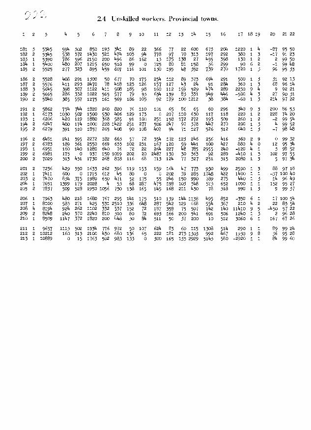
09 66tgTTo?6?-ogcl1Tc6?6? ÇcTc9Tooc0cdcg6?0cc9LTcT06990TTcT?gc69dg6oc6TL911?66cocL?T9T???99cT099oci1001?cTc09T?T?OT??T?i6669TT06?t1TcgodTcTT09cg1?9LoToc?L69LL11c6ToccTrLc96TTT?

9? L9L9TT9090Ç?OToa?LdocTic1goc9111100?o?9T?LcLIITT6ocgTOT?9? 96?dTOli?T90c169Ti00?991c69?Log0TÇoTgosl??oLc011?91j?9?60??? Loctrc6OTIITTOsiT?1iTLoccLgccL9T?L?cTLcc?cc?OTT?9?li?6si6Tgigo?ilcg??11oT?L9999 6T ?1cLg?91199cc oTc? Tccc?11TL?cgc00T9TLa?1OOT LTT90cc-cgc6i19dTT 11T6dToTccLTTIiTc6?L9L099T9T?0911c96LT90?

Ld 666dT066gic8LocilTT?99TsliTc91gdTocL9cOT Oc6Tg?c60cLcgL?co?L?6?cTTT0601?c9cLcgi1cdoTg6TcLi1Lg?99cc119?0?6LT66dTTc9LT110?611 96111dT01111cL?6gL066ocT911?cLTicTL110c90961Ldcg0L11L?co?o1 ooLc-TTOOIIT??119IILTcg?6dæ? 0009ci1?T9cTLT0009TT11LT?0?9T L69gco6c6611oc6dLLL11119T6cTccT6TT96c?9?cc9T0cc6?il9c?L?TO?

td L6cdT090?cTcTc?L?cLL11?TcTL999TT9L9 99?odLT TtcTc6?OL? 00?c L6?OTcTOTtr6g??6c9cococTL911?0??O?6TOT OcTLd6ocLTT969?66T

?c 96cT110?T-011?cc6?cgL9iL??119????L9L011909?TO11T09TTc69Tg6Tid6?T011099L?tOCTTilh6c0?TL9TTc??OTcc9699 od? 19d6gTcgL9?L6i?d 66o6?09c9Tlj9c?911?d?T?LT11cc?LLÇ99?9T?L??6dTt?19119?96T

911 g6L-cT0119?Tc9?cL?TTL116Loti90T 069011c9?Lc9ToTcT6c6L?9?c6T?c 6611cT00?OL?L11t19LL6Lil?90cLL?Tc???11T 9??0001lILT0911L11?9?1161ilc 66?-?T09?6occ6T?L??LTgcTTc?001T6cgcg9d09916TT0?il90?9Tc6TO? ilL9???T0??9TTLTToc9OTTLO?ocLT6?T9011occ o0T æc ocoTcLT9T?6Tccg00?c6oljd96?09c999c9TOTOTT9L0?9 09?0?9T1111LlIcL?9gc?T6T

?? L6ilT?cT09119c9Ç?T?T 0016LT?6coi99T6919TcL?TLcccgcOilgc?o6Tic 06L?c11ooc-911416ti6icccg6dTtÇ9d66LLLc9c??OT?cc99?99?6gTT? ?66116Oc??69?11L116?c6cT?TT09Tg6cgTgocITu??TTLoc96ccil9cÇ99TilT 9699dT09dlig?T611?ilL?TLcT9?Tc?T9111gLoLil?d6?TTII9Lcc?L9TcT ?6ccToocT6?1169dLd6g?TTuc?cLTOLLL9ooocT16?9011g?cc?99T

cc c96ÇTo?LTOL?6dL?ccgi1c6TocTTOT9TTLo96c11c6gd?dLL?c?cc?cgTgi1 66T-?90666?9cgcTT909c?L066gToc9cT?TLO?0911°O11T1191oc 66??TOdTg6cccilL?gdlLTcT?9199961100?ocT?96c9gL06ccTcgTd? T6LT-dTogd?6?L6TcTcOLL69LL116coi11L11T?cocilT?Ld9cccucc??9Toc cLg-11To??T110?dL9009??LL99d??69T11cc61ocg?odh6ccucccT9T

?? T?0?6T 9TLT9TclilTT?TTTOT69L9clic?T

SUO jt!DU!AOJf»P°PI1PP11f1,-1''

19518314 2121142530114142146 057 676518145 10101 1140146 05514720 3 1889 120 70 667 3 370 58 65 14o 63 11 57 75 146 1410 14 14 11 9729

21 5 1898 85 132 660 66 1148 66 39 165 149 108 76 20 90 1430 1 6 1 98 14922 5 1916 89 1144 936 79 201 142 16 99 30 28 148 192 23 -1410 14 0 10 93 14o23 1 1967 0 0 0 315 501 160 30 0 219 10 1814 3144 70 0 6 2 010053214 6 2030 175 168 800 181 1486 162 32 179 96 148 75 30 60 -3960 1 7 60 98 3825 5 20144 113 118 780 160 2148 39 29 18 143 12 12 63 77 1020 1 6 7 99 36

265 2051 10816562141131771451431181491330 36 148 52010 0985127142068 159114581218127076149 39372871100 65 21095 0991472814 2081 125185101403018970142 2151 717 214101 -14015 61498382952093 211162 520 0208781281614140140328 88 57 92016 18145030142116 58137671422215170145 63714761314 79 69-26015 799147

31 5 2190 213 151 780 52 207 37 15 83 37 114 17 80 145 910 14 0 70 99 5032 5 2200 111 1514 8140 147 125 26 21 96 514 9 814 151 148 12140 1 6 -99 99 133 14 2223 135 196 600 50 238 714 26 1439 56 141 61 2 126 380 6 5 -16 98 149314 14 2236 135 170 7514 51 238 55 35 52 79 39 206 145 97 11440 1 5 59 98 14835 5 2260 78 97 600 10 3147 109 25 186 56 8 92 1314 55 8140 1 6 214 98 142

36 14 2263 207 1140 650 325 57 30 0 35 2 21 1114 257 76 2170 1 5 -142 98 5237 14 2283 279 190 700 714 176 1414 29 52 65 39 90 6 71 -360 9 5 -176 97 5038 5 2320 155 171 7140 101 98 714 60 79 71 35 311 332 1014 670 1 6 -62 814 14739 14 23514 255 168 630 65 273 63 148 188 68 8 126 60 614 1170 1 5 -75 91 145140 6 2355 14014 209 6145 66 101 147 19 0 50 20 1143 12 63 1870 1 7 -78 92 145

141 14 2386 360 250 600 100 161 65 26 122 52 29 199 66 1614 330 1 5 3 98 148142 4 2392 182 138 900 139 236 69 144 266 50 73 17 1149 814 230 1 5 0 97 52143 5 21403 0 2514 1000 0 301 60 103 1995 88 1143 111 133 144 -10880 1 0 110 69 55144 6 21418 1142 136 620 100 219 71 56 155 144 28 1140 26 66 2110 5 7 -29 99147145 3 21421 328 1426 780 82 105 30 56 3814 59 143 55 200 105 270 1 14 -51 98 514

1461421436 2005090012323081149 936014191101 14o 29015 09539147 14 214144 158 221 575 237 1149 140 66 217 92 59 271 5 108 30 9 5 59 92 37148 14 21451 305 276 750 111 12 147 33 1148 38 51 122 60 53 -1310 6 5 161 98 50149 3 21458 13 190 607 71 290 78 91 263 59 14o 227 52 62 1140 1 14 145 97 150 3 21471 187 251 627 153 241 37 103 186 108 214 1148 27 75 350 1 14 1 90 55

51 3 21499 192 87 827 65 96 614 20 1497 145 27 189 117 80 140 i 14 0 100 5552 5 2505 128 160 8814 103 251 59 Ill 1146 68 29 82 279 51 580 6 6 59 81 14553 14 2516 200 220 715 56 251 76 20 140 144 20 36 167 14i 1090 9 5 -38 99 1514 14 2521 130 209 1050 82 11 11 514 144 140 15 514 22 80 2350 9 5 9 99 14255 14 2525 130 196 875 jQl4 366 72 23 335 53 35 105 1142 126 280 1 5 0 98148

56 14 2529 220 227 900 1514 355 142 38 17 59 37 121 37 60 260 9 5 -92 93 2957 5 2535 305 191 850 158 509 58 38 147 514 35 38 56 67 60 1 6 10 99 658 7 25514 118 1014 1429 199 595 61 32 105 1143 114 251 1514 814 1160 9 7 37 97 2659 14 2562 272 207 936 216 258 514 37 28 148 36 55 914 65 1020 1 5 57 914 14660 14 2575 62 2214 900 117 197 76 58 503 68 30 205 144 96 -360 1 5 370 91 14o

1 2 3

3.2

14

Lower public servants and salaried employees. Rural districts.

5 6 7 8 9 10 11 12 13 114 15 16 17 1819

1 6 1137 190 117 667 38 166 70 30 17 145 19 86 0 36 -3880 6 02 5 1183 252 78 610 0 20 12 0 0 5 19 72 20 29 580 1 03 3 1298 1140 109 533 53 147 149 33 11 39 9 36 145 91 150 1 14

14 8 13014 1147 107 3145 32 179 39 214 1144 20 3 14 35 27 5140 1 75 5 1319 14 159 500 58 230 60 19 141 14Q 21 31 12 32 200 1 6

61413314 0120637519814126 23303327 60 143 120157 5 1360 188 121 1480 37 26 13 23 122 16 0 814 120 27 1120 1 68 6 11426 137 167 600 3 112 145 53 7 141 25 146 5 52 1490 1 99 1 1509 0 0 0 225 269 130 0 12 21414 15 1143 37 57 -50 3 2

10 6 1512 300 198 520 20 109 29 100 1714 514 142 2 52 214 -2770 9 7

11 6 1592 255 158 607 27 52 32 142 214 36 5 11 21 141 1150 1 712 6 1680 89 120 520 14 136 55 39 31 27 17 114 199 26 2510 1 713 1 1687 0 0 0 50 2149 158 5 5 1514 2 179 1420 68 0 6 2114 5 1716 120 112 6214 162 113 149 141 126 214 31 217 16 32 290 1 615 1 1728 0 3 0 365 5140 135 130 0 136 60 96 25 65 0 1 2

16 14 1777 109 131 892 28 275 147 20 56 33 13 73 17 130 -80 3 517 14 1781 209 1814 550 22 13 19 78 19 33 7 29 25 714 11480 1 518 6 1785 193 1149 563 21 82 27 15 314 14 7 ii 148 38 2260 9 7

2 3

20 21 22

1408 79 14716 86 600 100 530 98 1420 98 149

010050-60 914 50-76 149 37

1 87 60-25 72 144

-36 99143268 99 148

9 71 530 98148010060

0 So 20-97 98 52

-175 95 1

20 21 22

3 96 1471140 98 30-2 99 145

781 72 36-12 88 42

269 99 146289914930 98 536932788 18753

-11. 9137

999501014 59 145

3 82 1431 97 148

-153 9550

153 97 146-141 99 14325682114

791427914 120198829822825126 67662977180 70163095 -899914280 14 2795 190 198 900 101 186 714 58 197 147 16 239 2 70 930 1 5 14 98 146

81 14 2803 332 228 750 215 266 69 63 275 814 33 2014 189 38 590 1 5 114 98 5282 14 2811 316 162 8145 99 160 88 149 1143 714 39 111 79 77 1500 1 5 38 87 14383 3 2818 1470 232 833 148 261 33 32 2144 62 148 33 33 51 730 1 14 -26 99 52814 14 2821 225 2146 985 117 206 88 148 138 141 149 1514 85 78 770 1 5 50 98 14885 3 2822 210 222 800 28 1614 214 62 1142 148 21 143 93 65 -30 1 14 135 85 23

86 1 28214 300 3 0 63 6214 2143 6 39 218 65 218 362 56 70 1 2 14 98 514

875 2833 797621411421.1462821 8627 01682146 605520146 -366146088 14 2833 129 183 1050 37 14o 96 65 172 57 14i 161 87 38 770 1 5 98 97 3089 3 28140 6314 383 1250 0 51 22 62 116 57 514 215 603 27 -2700 1 9 661 33 5390 3 28140 222 220 880 148 3114 133 51 57 63 17 113 1013 1714 -1820 1 14 72 98 38

91 3 28144 389 77 953 87 19 67 79 138 83 0 68 138 81 1220 1 14 -201 98 14892 3 2853 200 2714 6148 250 206 86 30 72 67 143 129 1251 105 -2820 14 14 3 96 51493 14 2862 215 256 700 5 260 39 314 163 53 28 1214 87 137 2150 1 5 1146 86 141914 14 2906 1450 814 1170 0 395 115 32 170 76 0 130 90 57 -f40 1 5 3 86 14995 3 2909 1140 272 833 107 2143 70 55 172 78 714 191 5 118 830 6 14 -2 98 147

96 14 2920 109 301 960 179 2149 119 143 229 53 86 269 90 72 -110 1 5 10 98 14097 14 2973 359 186 915 1144 229 106 27 155 73 88 239 91 91 570 1 5 3 98 14298 3 2977 309 252 750 2142 189 28 135 100 52 65 386 123 63 230 1 14 8 100 5299 3 2978 50 65 1387 78 376 67 30 176 814 51 278 97 86 210 1 14 5 97 h4

100 3 29814 201 2014 10147 102 2146 86 63 209 102 257 14.4 113 102 210 14 0 13 98 147

101 1 29814 600 0 11400 148 282 55 71 10 88 0 759 8 65 -600 9 2 29 100 114102 3 3001 260 2140 750 120 26 314 106 3114 88 37 1814 2514 83 1480 1 14 -6 98 531033 3022 31321880091171106 144 500922296200 7211140214 82971491014 2 30146 300 365 1260 77 1914 614 33 58 55 53 68 136 253 -110 1 3 8 9926105 14 3057 170 173 975 202 1114 146 72 92 55 97 305 15 111 2100 1 5 -11 98 52

106 3 3057 3714 14114 1251 2214 50 63 614 252 55 13 37 570 71 1610 6 14 2 91452107 3 3069 158 135 900 206 3714 76 85 187 119 68 297 96 89 710 1 14 2 98 52108 3 3069 275 283 607 72 177 65 35 80 18 0 63 67 76 31400 1 14 -145 914 53109 2 3070 683 290 10140 1450 1442 31 140 181 53 137 100 159 81 -1000 14 3 10 99 144110 14 3076 3114 220 910 138 191 63 103 17 214 68 98 30 113 2080 6 5 -3 89 39

1113 3098 318 335 986 267 14147 98 87 611.149 38180 136 96 300114 09851112 2 3105 0 0 14 0 14714 56 19 12 75 98 1151 117 90 11420 5 9 1 99 60113 14 3111 105 1914 1102 167 218 71 14i 60 78 27 123 26 148 1510 1 5 -13 93 14i1114 5 3135 211 211 528 3714 191 143 914 6 67 32 293 275 56 3820 1 6 -50 Bo 37115 14 31145 536 2714 8140 135 361 56 140 103 61 22 514 327 60 220 1 5 -111 92 143

116 3 31145 10 135 1000 83 138 53 0 310 12 82 128 1688 75 -2060 14 14 0 98 53117 3 31149 670 2147 607 110 169 57 147 136 72 26 26 67 83 2030 1 14 -12 98 52118 14 3151 550 236 913 125 250 39 36 327 78 28 2314 105 93 -220 1 5 2142 99 '44119 14 3157 12 130 900 212 317 100 21 239 65 27 3014 185 914 1600 1 5 -9 99 115120 14 3169 6714 1714 8145 81 112 146 28 97 32 114 131 0 83 11480 1 0 1614 77148

3.2 Lower public servants and salaried employees. Rural districts.

14 5 6 7 8 9 10 11 12 13 i'4 15 16 17 18 19

3214 261 837 63 167 59 31. 53 38 15 162 2145 80 1090 1 5178 201. 913 165 299 714 143 1438 1014 141 275 122 127 -2670 6 14

225 261 900 157 162 214 147 1145 56 314 206 170 76 330 1 5395 227 936 144 325 53 23 21 147 314 61 2535 35 -101470 1 0219 10 600 172 125 149 147 3145 814 38 1514 123 171 120 14 14

0 124 750 37 2146 514 7 83 62 51 81 253 72 21450 1 52371937508319092 1414 80575119 2148 141151015382 192 1000 0 63 80 70 1140 314 22 81 17 76 103 1 14

280231 900 251599360 395132129117 68 220 141062565201.53278888156751451479 80 149 770352552929561141114997147 1h14 863141314102 95 214015209 211 10140 102 2614 38 314 96 143 28 18 300 145 1930 1 0192 251 5140 1114 14014 92 52 106 103 59 77 0 69 2090 14 5216 237 512 291 1014 32 88 121 66 514 177 286 71 8140 1 5327 282 675 276 128 50 52 130 72 23 150 17 81 1170 1 5

309 231 510 101 1514 70 65 132 142 33 149 76 93 3730 1 5283 238 607 172 321 72 36 52 85 29 67 67 56 18140 14 14

350366 630102355 71713150147514 145 90 1450143

1 2 3

61 14 258862 3 263663 14 26149614 5 265265 3 2667

66 14 26786714 27014

68 3 27014

7014 2711

7114 271272 5 271573 14 2729714 14 273175 14 27140

76 14 27145

77 3 2780782 2783

ç9çi09TL91çl9iLO009TtTO11TOGT99L9.9OTT9tl991OOTT 9i 8LLço116Li6l ToeLci OTTT 90T089oT0601Ç2Ç91100119L1Lf).T9T9119Loi1119Ç9tlfoç1001111LLiç186Lucçç1lcTtTOTL1l91cooTf6ç9L1

li01%ç8T6111OLi8i1911o9ç616cçLTlç1LLçcclITocooL199ç111L18Ç 69çL9L6LIÇ6919oÇiIll09T1199ÇLT911ILIT196911991091ILOTiL0099911LI

9Tç11T001911101LLÇT111191ooeT911T81ILT

L6696909ILl 6i OOITÇ0916o9ç1OLT991o1L96Lt1çç o1 11ll6L1691

GL11111169o06Ç6ç9006çlççç11oLL99TLLT668T1161L9Tgi061ççgoLllIToLLçL91ç9911aL910T 91lOTÇlÇ69dcLTLc991

91Tçç9LTOITççç1991OO1TLç9T1T8166çç1L6ILl001 0066li6Tç99ç111191199619L11ç11cç01010196ço6T8119çç9T

T69cL91LiIL9LToio9L091Toi119919T9çiTTLioLLlçLTTI96109ç99ççT91

9L1191119).LiLloTog6T iz L9z6T9ç11091OiT61OTTOTTTiL0LT001 0lOTc111oLlo9ç 6T Tl9T116L919ç16oT66L69916L69t91 Lç1166lI6LIGooç9ç69L1101LT6911Gg69Li61cç OlT 9616L1111ççi 9T

8çç8118L099çi911111TLZTT8119lç11ççITc9iLç9L91Logçi0111961ç11ç11T

011ç9ç16011901 69 6090oollTçcoLl9Ttj0lilT91TOTGo9çc11oc1lOTLi9L99Li9916T090966109i0çç TTç11ç66çTL1169çççççijgço9ç10çoT çj1199L69L90981119T O9il99g6iÇ1611TL811Ol9L611æl Lcioo1 d609TLL11Ç811 ç0çL611Ç9ccL111LlTLT6TTLçLiTL11TLOT99çoT6L9166ol LOTL91-19iT

91L9)2OOT96TILT109L911 091L91cçiT8109Th1ç6L9i1OOITLilcil911ç 1l 091186118LL19111108T 9l t$JTLtttÇ

f91TcifTT8111I1ITOT69lL6161iÇli1T9I çç01119169T l9111Çç111çTT

TLÇLL110119L9LL9100Ç0LTT LloT6oc11OtlT118ç11L60001it086T9Tc01168c1L11To+cc6T ç918TLTOT1919LL2ooçc6TLcçgc-011116T11L8iT91.LT9O1TIQIcc19ççç LT

Tcç96611001-Il6TiOLçl90T91OTO60691i1ççooÇT9çcI9cT9i 669).-TocT11611L1Iiii96TlOTTIT09ço96L081iTif66çT09690T98OT TT11ç1811Tl6TT116ççTTTT1fçT

661TtT019-1Lç9TLtÇ9LTl9T119gOT 00116L1i9occcçç1966T-111066116çL61ciT911TTL0696Loo1TLliÇocçi66111oie-I999TtT699LcLiL006TIÇo118TT

11Ç966119O9ÇT9LolO9L6L19TOT1TT0OOTOlLll9ÇÇoÇI911 9661fi-TOÇT19LL9T199TLLol 9069TLT6i9I11611968 11111oi1oÇ9L99T9iOT9119T11OLOj991101191lç91TiTtl 69OI91O19O9OLL19i0119TT6Lbl690t196iTIlççLI 911 96i1-to6i6LLTiTLi68919T1610001 9T9l911

Li L6l1Ç091OLLT9118l 016T9911°OOL11819T6ClT1TlL611911io6l61LToçct69L11T*998L8dTOÇ1111L11 6L90TTo6L6TTLLOlÇ

116T96TT10tO1LgI ÇÇcgTcliÇl1l06LlTO96Çt08t1998L6111TT olT 9l 9t1911111lL6lIT-l10911T6096LTT61Ç11ll9Ç O1T0891l 66ToLTT1T

TlO6191LI91TTlI110169L9çIT

S1ZTi1SLp P}10Tdfflpui S1UAJQ zqqnd iMO'J

ti969TTOçIIIi9L1T0901-oT8LTTL6c608-L9106

9ç 6691-6O9TTOTTl9tÇ L6z-116019-6LLoe

Ç609116oe696ZGc L).19Tci oiLL001il 96911111600001191LzL2ÇT096LO

ç11 116191011Ii19

çL6911ToLç-89LL1o96ocTo9tT16Tg6o-ç9oç6i961L9

86iii O9TL6oi9iTo69T08çTT

1ç 969111T09996ccc9ç ç991T0çç1199

8L1T116019ILiT911 LçL-OT0991ç8lçç L6811ooi8lçç ç991io6L91116L116901-11TO9116881911 9611-i o6901LIL66L11T0911-ITT98).811 f68ç-T01111691G

91 96T-tiOitIL99c11ç6911iOlcTLL911 66TTT09ç6991c1 tLçTzçToç8z-8919OLT

0986il116o11Tci

0966611110916IoOL61-ç6OL1TT1Tl

0116611T0T6L9o011 9Liioot1lT811 ceç-cT0L11TL001

i6611190919).ÇÇ

Il66tiT O9l89l8Ti 69OTIOCT-Q6611

i 86T009L9T111Z111 66991TT09hT

09669-T0O11T

86T911ç O9*-6911Ç 666-111OToo6LT111oLI-9Ç

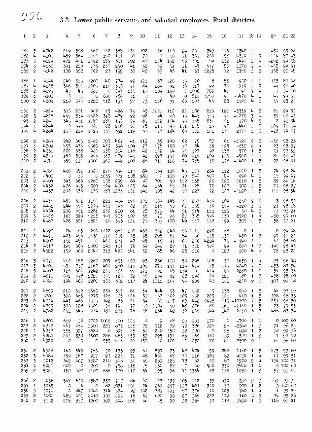
1 2 5 14 5 6 7 8 9 10 11 12 15 114 15 16 17 18 19 20 21 22

181 5 140142 219 358 667 162 388 156 102 15E 110 214 201 3149 115 13140 1 II _5( 95 26 182 14 14103 1489 3614 1050 150 131 60 70 0 56 11 353 200 58 14310 1 5 1114 87143 183 3 14129 1472 1401 1092 185 331 102 147 1714 132 56 301 59 132 11490 1 14 -202 99 38 1814 3 14133 391 219 773 237 250 141 32 59 51 11 148 577 80 1170 9 14 -68 99 51 185 2 141142 138 363 762 27 159 53 116 65 118 141 33 1298 72 1380 1 3 158 90148

186 1 1411414 2140 315 1200 140 7714 92 121 37 126 55 20 8 85 950 1 1 153 86 146

187 14 14168 366 300 1205 210 336 91 814 289 92 36 317 99 76 930 1 5 -9 96 140

1882 14195 140 143 690 06147175 10 109 109 01096 766 140 9099 35960 189 1 14200 0 0 0 600 768 71 0 0 149 0 815 3750 97 -31470 14 1 145 99 55 190 2 14209 219 375 1200 118 153 97 73 166 91 66 193 145 88 1520 14 5 35 9825

191 2 142214 300 201 962 13 1428 75 14 2620 112 22 166 219 121 -3350 14 5 21 99 55 192 3 14228 1455 3511 1522 315 1479 92 92 911 90 15 14145 515 944 -1270 5 14 39 96 145

193 2 142140 3145 14i 1080 180 156 29 85 122 1044 95 338 831 51 170 14 3 2 91 514

1914 3 142144 0 3914 760 88 260 66 78 215 95 151 208 15 97 114140 1 0 109 70 514

195 14 142814 130 2114 1025 537 552 119 37 77 1614 63 501 101 150 2370 1 5 -28 71457

196 2 14289 2110 365 11460 793 1467 141 115 35 1140 62 75 87 61 -1720 6 5 -36 9823 197 3 14302 1458 1435 1560 1465 358 1014 77 178 120 97 814 16 128 -650 6 14 23 98 37 198 2 14i 202 558 960 130 2114 118 142 152 6k 91 327 92 158 370 1 5 51 99 52 199 3 143514 180 33 j67 579 1145 142 693 151 60 215 109 116 -500 1 14 86 96145 200 2 14576 585 216 1500 167 1498 105 86 711 116 7k 788 30 178 -11400 1 3 72 98 51

201 2 14386 1406 382 1560 270 5514 110 8k 3514 106 145 177 2614 112 1060 1 3 714 98214 202 1 141403 0 10 0 1035 571 108 180 0 103 79 8140 500 8k 690 14 1 15 99 k 203 2 1440k 3143 566 1260 156 259 814 90 701 59 112 158 20 126 1010 1 5 89 814 114

2014 2 141452 1476 ki 1500 129 koe 125 8k i14 85 21 128 70 107 500 1 5 77 9827 205 2 144433 202 536 1175 387 1233 161 1141 508 92 30 227 72 127 -1120 1 3 111 98 314

206 2 14456 1485 511 1150 221 kk 196 101 369 1148 50 257 1435 109 250 9 3 3 98 52 207 2 144141 2144 550 1275 k 593 62 65 215 50 67 158 30 1514 -120 1 3 21 98 18 208 2 1414614 256 1451 1281 23E 200 81 28 579 614 51 5114 111 115 30 14 3 73 9521 209 14466 167 520 1215 1145 205 107 56 70 96 27 358 59k 139 2520 1 14 -30 99 60 210 2 141487 1426 501 1821 90 393 121 71 559 100 149 117 112 99 300 1 3 58 97 21

211 1 141490 2k 63 250 1622 885 150 352 2140 55 1115 290 68 0 1 1 0 99148 212 2 141491 ko k6 1630 110 239 78 68 298 81 8k 50 113 130 ko 1 3 97 9622 213 1 14507 152 1481 0 1466 271 147 98 16 97 60 206 1422k 75 -13ko 6 1 66 98 60 2114 2 14517 195 365 1300 1143 131 76 59 2149 29 71 302 590 99 850 1 3 1146 98146 215 2 14522 159 366 20147 513 1426 1141 52 88 146 98 116 0 128 160 14 5 78 98 22

216 3 14571 klo 188 1267 205 633 120 93 256 110 50 298 108 57 1650 1 1 25 96148 217 5 14601 531 737 1167 1406 260 115 105 275 131 1114 1419 15 115 142ko 1 0 -53 87 k 218 5 14607 126 361 12142 265 566 99 171 91 65 139 91 1419 86 2280 1 0 314 95 56 219 2 14671 602 598 1820 555 125 72 56 239 92 68 196 66 121 580 1 5 -38 98 60

220 2 14680 1914 1460 1200 163 302 117 2k 1511 107 914 209 145 161 -260 9 5 107 99 18

221 2 14699 210 312 1560 2514 515 81 314 1414k 53 147 1142 5 158 9140 1 3 1414 97 19 222 2 14701 590 665 1275 126 505 126 59 157 102 105 158 225 121 klo 1 5 108 9823 223 2 1472k 1447 k6 1515 1142 83 21 514 53 117 69 14142 51498 115 -10500 1 5 251 96 50 2214 2 14755 300 228 1500 26 195 77 50 2509 50 148 276 80 161 -1160 1 3 25 79 55 225 2 14782 251 5145 9514 186 255 78 58 23k 142 32 205 514k iko 2650 6 3 1488 83 sk

226 1 14800 659 36 1762 1066 500 123 0 9 68 15 953 170 0 -703 1 1 0 100 60 227 2 14852 1461 147k 1500 221 875 155 78 912 79 72 386 326 96 -23140 1 5 71 9825 228 1 14857 555 397 1620 0 395 145 51 2140 150 32 180 0 95 890 1 2 50 9938 229 2 148814 281 s8 1500 288 k6 159 59 295 131 65 169 160 139 320 1 5 1 98 50 230 1 14920 0 0 0 555 1416 20 150 0 102 10 232 170 81 2500 9 1 66 96 60

231 2 14928 160 5149 765 50 135 93 61 597 75 148 14014 55 288 1160 1 5 275 93 60

232 3 149814 589 187 917 97 225 71 148 146e 68 70 116 505 82 14950 1 14 17 99 51 233 3 5012 362 1467 1587 210 503 51 65 259 125 78 32 68 87 1920 9 14 1314 10051

23141 5020 600 0200 0758115 75 15087 0140 50025021414011 810060 235 2 5021 150 1407 1100 686 570 117 514 195 96 72 i6k 62 115 1030 1 5 57 99 k

236 2 5056 567 610 1380 350 717 86 ko 127 139 105 112 39 350 350 9 3 -149 99 514

257 1 5065 0 6 0 821031 151 2k 269 257 197 1421 310 70 900 1 2 31000 238 3 5071 0 6147 10140 3114 5k 92 1142 789 191 57 376 10 103 780 1 14 1 99 514

239 2 5100 1485 1401 2010 103 295 18 61 690 99 27 165 222 119 160 14 3 76 9528 2140 2 51142 215 517 1200 192 208 105 66 k 52 55 556 57 118 51490 1 5 118 99 21

n /) f 3.2 Lower public servants and salaried employees. Rural districts.

sz.i1s!p punJ s(o1dui pzuiqs pull SjU11AJOS zqqnd iato

ZT Ot39gLzccT99cTLLZtgLLLtzooc0003119TOOZT09091oocTTOZTT99zTcoÇg93L63T6ToLlz6zLIITT 0096100911c9OgT66331 0303L).c636T911313ZTOZhOTcITccccLic6cTcz001ccogig6zTT01111133cczLTd9188363cgT96zg 6Li1zLT3do9ct166LTL6zTToL99111goc6igT 196L0010Idz6c009czgiicc6LLoi6L1963

TTodLT-9c369LcgL6ToZL6z011itjdILTdg9ocZLI91ocTÇ9Lic6zçToTc9091L0ccz).LTTLcOTT91TgIL9gdtj6OTcgcÇi1t1L19Lz163z016T9gc66119T9699ZL111LcT90c1 cc009ogc3339911LTd6316oodcg1111gcodOciLcz19odi083960T 091 cdl Od19otLIz6zTT03T3366Lid6gcz6zoLz6oTccz930T czLi93009OO1LT163

31odldLLOTOLTT dg911099zd6L1d09ozLoocT6cz9d1ilgdLIo6zcTod?903003zLc6g9c3czz991ciT16cLTcodLT1d9903oddLz6g?cToLi1-'13ddoz99L1 gccdczcc6c1 dz oldIccc9d3LIILzggzzTo6dIcilcgz9001 969LI0036999TTdlcddcljZc009c369L9Zz9o6ccg901d61LzczIdz089?T9LLT ozczL1008c393069T983

dTo6tLdTTtjd631ddTdT903T9301LLLgc0166Ld9L38189zdgzdIoiL1-10d69cdzd96ITTzdTIocTccT3990190091icz9TiLZL9z193Çocz931czz606T93TT?66i1Çoo009oc9TzdL9113L699zdgzd10691L8TLdLcg131td19ciccOTz6T600919ccdt1900993393zT096-631ooddzTT o6TdTzcocTLTd61dL66LzcgLizid0096gc91183

ZTOOT?ÇIlclTocgtlliTLizOiz09czl6d6oooooLd91093ÇI003ccT39009oLIITT10390319998czzc9TTzLdldz1L19z6Lz1ToLccL9TdilL81 39iLdod61gz6cT6d0011LTdOT919çgLzz6OOT1130190110001 dIT 6gLd13900011cccoldd1119TLLzzTOIITI1801gzzddLocc6LT6d1OoocTgdZToO9Tcc9I9)2

ÇTOTZ-LLT6odol 9c1cI16608LL9cZTZo9cITod69g110d9zcLzZTOidLzz0900?01OcTT16zTZTT 0ccOdzI1LTogc6z9TilL?T019T- 0T9lzzIZTT dzcoloiTTITTLoiocTcOL?ZT099higz9TdLzcIOL1ILdT0?T9dT9LicIIdIdLog6zg09000?L6dzLd199z?LZd60)23zdTocLL9z19Ld9139c9Lzlll0011g9l?1Ldz9ZTLZ

çI09c16c1Tdd991116IcTcLcdoT19Ticc1110031zcdcc93919zOL?çLO9d?cc961cccTT631dgl6g19T9LigdOocI3111T6cT1T93693T6o9dLZT9g?dITild6cT916TLT6dTIczT coil063199cg?6119T99?cTogcicilcilzcdLci?LI0110119idILlcLz0031zoczccOT9zL9zd6oc9goeLdoz9198?O1?8163919gd0?dT6Td0161cgo9399?

Iood-6611ogd061181IdIc191zc01196gL69o?d6L?ccl1909Id9?zT01109cLtjLzd0?901L96c9ccz1d6090600099co9I19?zIoz-d6?dolzcTczzcdlT9d6LIT001lcd011999g9od9L6dTc9?dTO9TT6cTcc031199L?T88Lc??3dLoiTo?cL?Tcci 991Ld6d?39?zToldZTZoc?CITIdIz6?lOLl/21dzT190T O9odTid? igcccT19?

ZIood09889cccocLoc31OL?Oil0ccOo?dI0091c6gcT09?T0011g1Tccz0391 gcd6c6Tccl9gTill i6oî ogLgzc6LgcT6czÇTo6cz631913gggdL9601?6cdLd9?Lci0031d?l ozd6dgczgc?çToigz611lgdogdO9ggodTzicgTzclOTcz6cc?0??66Lc?Lczz6ocilOOzccoLlgLcgzL6d011L6z01IOI i9d0L1T0009LzLdT9/2

1T090?T6OL691gildI06619111091913990116d9gg9cçdczdTOTtjIddz61Tg??d9ccicd?901l19909ddLdTgzi0096c9cZid?160101911Z?TITc9ddoT161ccd6911gLdz 006ddzdodgiccdcczoiogzg96d9L3111LT08991gd901169dol/2966101?93ccilzczd6o9d-odiccT9d9399lid?czdgl gg 813dIT0/2LII13cc?Ic?

160/2OzTOL?1TLocdTT88136g9TTT 9L99TLIL91006dIldIod?TO09019dTLlzgIldd1910Ldz996/261?dLgI9Toilcdiçd1611?o60901L6TTITTddZTTg66Lidoc09?dgdcgol96?6og9?ddd81?d109L99To6zizdzdg6o?d08dITdoizdloodT6ddTOI1?dd?Li?ITO?LgLz9LTogiLz3d001903gLL901ozdzoozioodd191?

dTOTddLCOTdLTdLgLL?d9/2i?TT9d991009T6zd139g6?dZd?d60166dT01dzlodLgddlidcgidddoeOT1TL99/29i??c?90?TIOd91OoLi1d?TLTd?TIogTdTo9o?LoodTo009OT?dIci? T6 OIIILT091zodccpz dLd6ddcio?Ldd99LLddocodldT?l?ÇTO9OT-ddT9dldÇTgLd01zgtdddgzodzididIdLdlTdZTi

6T giLI9Tdl11dT31TT016gL9dild3T

09 19oc6i 66çÇc z69018i L661id 66oc

ic 66cc?L6oi91 i66cTzc d60ild 6631-

dd 66009 96dzLz d6911gz L6dd8i 96Lgz

dz cgcodic 166-1? L8Igt 666z-LI g6Ti

1c66661 OOT1111 T6dT

1OOT 9Tdg6 9L1

Li 061101-61 66T

oc ooi Lc13 z6czz91 OL01

11 666d-id 66czTcc cco91d6 gdcc CLtIT

dd OCT LTc 6601?d c9c69dl 66TITTd 66z

09 66ii6i 66zIc 6L6zcc ogzgîTc g6g

od 1gÇgz6d g6c?6z 86IL31 cg90dcc 0010

09 16oId 9669di 66It-dz 1696i d6o

61 d8L691 d6oco9zgodd og911dz g69T

zz 13Oz

( ()j -(

2 3

3.2

4

Lower public servants and salaried employees. Rural districts.

5 6 7 8 9 10 11 12 13 114 15 16 17 18 19 20 21 22

301 1 8105 600 18 1617 Ii-82 816 196 0 375 169 114 1257 1000 207 520 1 1 40 99 60302 1 8230 480 120 1540 0 737 93 34 52 87 0 859 9824 201 -6060 1 1 -29 98 54303 1 8318 571 777 2650 81 887 167 816 1475 29 160 309 2140 188 590 4 2 50 99 3143014 1 8368 1086 594 1700 21 837 121 183 1421 201 70 939 180 188 270 1 2 14 98 146305 2 8407 2141 732 1050 620 625 178 81 11 107 45 760 321 183 2810 1 3 -98 94 58

306 1 8565 0 0 2224 706 1778 149 64 2559 309 18 3177 1495 75 -4020 14 1 71 100 60307 1 8587 569 4814 1500 893 1188 151 628 70 314 186 400 1188 415 -1450 14 2 -62 100 47308 1 8992 7147 898 960 38 290 71 89 1014 98 192 503 95 150 4690 1 1 _314 78 60309 1 9077 420 250 2310 400 824 180 196 0 124 675 760 2703 522 -800 1 1 914 96 47310 1 9191 300 1458 2026 814 1231 196 122 595 283 472 993 483 139 1410 4 2 159 98 45

311 2 9216 369 310 1300 375 771 60 150 1858 1445 325 703 1830 169 1250 1 3 218 85 514312 1 9325 576 65 1815 530 878 190 120 28 183 50 20614 780 213 1310 9 1 20 86 60313 1 9326 588 121 2012 1261 902 111 295 0 168 8 1147 263 5314 790 1 1 20 99 603114 2 9335 425 856 1788 527 721 84 110 69 236 37 1910 0 232 1100 6 3 7 9932315 1 93140 14140 350 1800 10140 1975 210 350 8205 205 10 865 520 200 -2650 9 1 30 89 55

316 1 96814 723 1400 1092 20 688 65 152 285 40 66 355 21443 166 3050 9 2 3143 86 35317 1 10289 1037 8147 11440 1435 769 28 86 35 167 202 502 136 235 2020 1 2 137 92 38318 1 101447 360 0 2220 530 11498 228 277 325 193 555 1006 6298 200 -2190 1 1 50 100 514319 1 10913 1480 120 364 o 1498 187 1450 0 2114 58 398 1080 1436 2820 6 1 81 98 146520 1 11079 936 898 1960 7146 717 228 396 272 1814 62 148 5666 218 160 9 1 314 100 89

321 1 11782 602 1164 1200 260 375 181 296 1362 166 68 732 2140 220 3690 1 2 79 95 60322 1 13498 360 3614 1800 70 16149 2145 68 1026 209 196 1511 21425 1428 1810 1 2 208 89 142

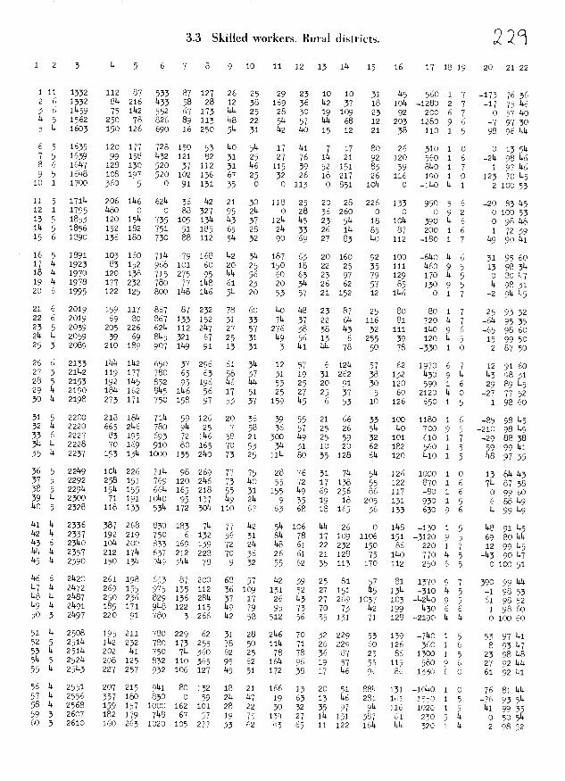
2 2920 21 22

-173 76 36-1775146

0 57 t47 973098 96 1414

0 13 514214 98 t#6

1 97146123 70 t#5

210053

20 83 450 1005309814817239

149 90141

31 95 6013 983140 80 1474 98 31

2 914 145

25 9332614953565 98 60159950

2 87 50

12 91 6014 983129 89145277752

1 98 60

85 98 1#5210 98 14929 88 38

59 99141148 97 35

13 814 143714 87 38

0 99 606 88 14914 99 149

148 91 14569 8014412 99 1i

l43 901470100 51

390 99 1441 98 5361 98 521 98 600 10060

53 971418 93147

23 9814827 92 14461 92 141

76 8114476 93 514

141 99 350 5051429852

3.3 Skilled workers. Rural districts.

1 2 3 14 5 6 7 8 9 10 11 12 13 114 15 16 17 18 19

1 11 1332 112 87 533 87 127 26 25 29 23 10 10 31 145 560 1 726 1332 814216 t#33 582812381693614237 18 1014_1280273 6 11459 75 1142 552 67 173 ti14 25 28 30 19 109 23 92 200 6 714 5 1562 250 78 826 89 113 148 22 514 57 144 68 12 203 1280 9 65 14 1603 150 126 690 16 250 514 31 142 140 15 12 21 38 110 1 5

6 5 1635 120 177 728 150 53 t#0 514 17 41 7 17 80 26 310 1 07 5 1639 99 158 1432 121 82 31 25 27 76 114 21 92 120 560 1 68 6 16147 128 130 520 37 112 31 t6 115 39 52 151 83 39 8140 1 79 5 1614-8 108 197 520 102 136 67 25 32 26 18 217 26 116 190 1 0101 1700 360 5 0 91131 35 0 0113 0851 1014 0 _it#Olil

11 5 17114 206 1146 62t# 36 t#2 21 30 118 25 20 28 226 133 950 5 612 1 1795 1i80 0 0 88 327 95 214 0 28 36 260 0 0 0 9 2135 1853 1201514735105131414337 12t# 14523514 181014 39014611451856 152182751511856528 2143326114 85 87 2001615 6 1890 136 180 730 88 112 514 32 90 69 27 83 140 112 180 1 7

16 5 1891 103 160 7114 79 168 142 314 187 63 20 160 92 100 6140 Ii 617 14 1923 83 152 968 101 60 20 25 150 18 22 25 35 111 1460 9 518 14 1970 120 138 715 275 95 144 56 60 63 23 97 79 129 170 14 519 14 1978 177 232 780 77 i148 61 23 20 314 26 62 57 85 130 9 520 6 1995 122 125 800 1148 1146 514 20 53 57 21 152 12 1146 0 1 7

21 6 2019 159 117 867 87 232 78 60 140 148 23 87 25 80 80 1 7226 2019 69808671331523133 7143722614116 81 72014723 5 2039 205 226 6214 112 2147 27 57 276 38 38 143 32 111 1140 9 6214142059 39698145321672531 1495613 6255 39 12014525 3 2089 210 189 907 1149 91 13 31 3 141 144 78 50 78 330 1 0

26 6 2133 1144 1142 650 37 296 61 314 12 57 6 1214 57 62 1970 6 727 3 21142 119 177 780 65 63 58 37 31 19 31 262 38 132 1430 9 14

28 5 2153 192 1145 832 95 196 146 144 53 25 20 91 30 120 590 1 629142190 181416281451146561751 25272537 5 60212014030 Ii 2198 273 171 750 158 97 53 37 159 li-s 6 53 10 126 650 1 5

31 5 2200 218 1814 7114 59 126 20 36 39 55 21 66 33 100 1180 1 632 14 2220 665 2146 780 914 25 7 58 36 57 25 26 514 140 700 9 533 6 2227 83 195 693 72 1146 58 21 300 149 25 59 32 101 610 1 7314 Ii 2228 70 169 910 80 165 70 53 314 31 10 20 62 182 560 1 535 14 2237 153 1314 1000 135 2140 73 25 1114 80 35 128 614 120 1#1O 1 5

36 5 22149 1014 226 7114 98 269 77 75 28 76 31 714 514 126 1000 1 037 5 2292 258 151 769 120 2146 73 140 55 72 17 138 55 122 870 1 638 5 22914 1514 155 6614 165 218 55 31 155 149 69 256 86 117 80 1 639 14 2300 71 191 10140 95 137 149 214 9 35 19 18 205 131 930 1 5140 5 2328 118 133 531# 172 3014 110 67 63 68 18 165 36 133 630 9 6

Iii 14 2336 387 268 830 183 714 77 142 514 106 144 26 0 i148 -130 1 5142 14 2337 192 219 750 6 132 56 31 814 78 17 109 1106 151 3120 9 5143 6 23140 1014 200 533 169 139 72 214 148 61 22 232 150 86 220 1 71i4 li 2357 212 1714 637 212 228 70 36 26 61 21 128 75 i14o 770 14 5145 14 2390 150 1314 o1 1414 78 9 32 55 62 35 113 170 112 250 6 5

146 6 21420 261 198 653 87 200 68 57 142 39 25 81 57 81 1370 9 7147 14 21472 269 155 975 135 112 36 109 131 52 27 151 5 1314 310 14 5148 14 21487 250 236 829 136 2814 37 17 26 143 27 269 1037 103 142140 9 5149 14 21491 185 171 9148 122 115 149 79 95 73 70 73 142 199 1430 6 650 3 21497 220 91 780 3 26E 142 58 512 56 35 131 71 128 2190 14 14

51 14 2508 195 211 780 229 62 31 28 2146 70 32 229 53 139 7140 1 552 5 25114 1142 232 780 173 255 78 50 ills 71 26 229 60 126 360 1 653 14 25114 202 si 750 714 360 62 25 78 78 36 87 25 86 1300 1 5514 5 25214 208 125 832 110 365 95 62 1614 96 19 57 55 115 580 9 655 14 25143 227 257 932 106 127 145 51 172 38 17 146 9 8 1330 6 0

56 14 2551 207 215 9141 80 132 18 21 166 13 20 51 8814 131 10s0 1 057 14 2556 357 180 830 0 59 21s 147 19 63 13 146 281 11 1550 1 558 1 2568 159 157 1000 162 101 28 22 30 32 35 97 914 116 1020 1 559 3 2607 182 179 7148 67 37 19 75 1314 27 114 131 387 11 230 5 ls603 2610 16026310201052773362 14365111221614 144 320 il#

3LJ'nLp jtJfl}J iJOM PIIPIS

oc L6lt1T0911t1IT00610Ç9L914L9L0LÇL9ÇL?99?6999?6ÇÇ0?I:o4 L6 6-99016?o9044LÇ0949116ool9j1Ç46Çot1OloÇÇ468ÇÇ6114c L841T04601- 99T9169064o14?TiL6944.ÇL98991?L969ÇÇ91194 969111ot??619911?109LL9Tt16419ÇLÇ491LoTI19?104498ÇcLIT11 Ç694TÇIOL?19??41c.40Ç99499969409414Çt1L4849Ç1911

4?999?T4T0619609169Ç999Ç6Ç691691001649?T?t1919Ç14T19Ç 96991t11009?8TL41991I0016L?ÇÇ001019ÇIÇ4Ç94Ç96?9ÇLÇÇ9119? 9L9?0ToL64419ÇÇOT0?6609911l4460001Lo4691T0LÇÇTT

69 161t1I O?4IIT181Ç88ILo1161414?11100119oÇo699ÇÇ11119 Ç64Ç41064?191L99011994441OLIllT44Lo9L49?Ç91099ÇtITT

99 46aT1601144TÇ44469?6499T461194Ç691T?T101LLTLÇ9ÇÇ01144 069ÇTÇTo?L-66?090???9001Ç0L94L6949OÇI0901919091?Ç9Ç?6014? 141-01OLOÇ99L4ÇoÇ011?90?41Ç14?1Ç090110??44?444190194 96t?99OL9Ç91691L94119?Lt1i1L?TT?10001ÇÇ?a6îo94ÇÇLOT

T4 L69-9ToLÇ60?0691:??L99991649L941090196??Ç4ÇÇÇÇ901

ÇÇ T964Ç006Ç9?0??9L0999901o446?441?O119Ç1Ç?401iÇ 669Ç96000Ç-46TÇ6o1Ic?o404??1?T414?09?4TTT19140TÇo9Ç49016946 Ç99T009?4410?LIT8?184LLÇ4L61ÇLITL9L99199??09ÇÇÇoT

49 66001-4909966L9L94141949?046ÇL6ToL610449Ç69ÇÇt1or?4 99?4t o-8Ç?90461Ç88949964TI?94?L09T4?L19Ç9ÇÇÇTOT

T9 L488-0TOÇÇIllÇ90ÇÇ?TTo480149?900?09?OLLÇÇ?044L?444OOT

?Ç 9Lt144T0999+IT1Ç?6TIL46o?L641111041694??9ÇTÇÇt66ÇÇ 46Ç6-9o9LI-LÇIo4LÇÇÇ?961199919919L?ITÇ1ÇL9ÇI19?ÇÇ96Ç1 994tÇ44-L4i419Ç90?469Ç60660?L91L?ITÇTÇ40?94?Ç44614 46OL99064?-6l411L9?ÇÇ9LLTÇLOT499L?99?Ç69141049O9?ÇÇ96

14 961?-t099LiÇ1LÇÇ?180T94ÇÇ994T9ÇT?LT6LI?44?9Ç?ÇÇ4649660990199??49?Ç4L999?9?9Ç?9Ç??4tiL9899?9???4Ç96T4 96TT009L416690T14Ç9L91949L16ÇÇL9964?OL?4I?Ç4604 6601-41o1ÇITT11949?L098?091419Ç99494LT?66?9O?Ç?6T4 16TttoÇ994TLL9OL60?9119?9L6?6ÇT966L99911?L9Ç4014ÇT6

L4 660??-96066194190119?ÇÇo4441T09T?69T6?9941449Ço?Ç40614 964L-96089?944601?99804TL494LO?ÇÇlL1TI94?9?Ç9LIÇÇ699096 L?604Ç0919L96?9L991OLI0800199?69?09011419LTO9TÇÇ88LÇ 66144o41ILT94694??9?ITL??4ÇÇ ?I466Çt1Ç969LÇiÇt4949 9969?910LÇÇ091ÇÇ?9T8?9494?9?4TO?1?To?L141Lo?6ITÇÇ99

0986 99T08-191ÇÇ001?449oL49966914L??Ç49Ç9Ç10?9ITÇÇ494496019109?191L?691964614Li1?4LÇ?LÇTL996??o6?9TIÇÇt19 961?440914919?4191901T669961?49TÇo4oTO?ÇOL?T6O9Ç9

14 96001-4099Ç1T01?494?99199L04491Ç?1L99099994o9oÇÇ?994 968Ç9TO4?Ç-9111691991?4LL9ÇT91969Ç 4ÇÇ11969T091ÇÇ0ÇÇ19

99 96494To4L9011T?91Çi4T916Ç9?IL4?06644?sioL?66?9094166 Ç1Ç90OÇ9L1?T90149L?9L?4?9L?0410LTI11ÇOÇT066?16L

?4 66oTT0L4L-11141OL??94?69Ç44?Lo4L19TL9?L96?99L94 96999 094190?99TT01OLL4hL096I ooi901LLI6Ç61ÇLL

Çt1 6LO?-410099T1199?TIOTL666116L006191094I9?i9L

0996491oL4?9TO80TLOLi6LIT T41?L994L1Oh?4?4 964014T049- æTI191 01 91199914iÇ0?T9900691 Ç9iÇL8?9L

9Ç99-410O1T4LÇi1oI66?4L16looz46ItilT??9??ÇL

14 6694T-ti609T1L91L14L?Ç19?9???9909LT9?T690???L94 66?9T01?9TLL?L99t1i1LOL?99?Lo4i0101lii?o0Lo91TL

L11 96oÇ41094411ÇÇo4i?4Li10?04L4Ll6?L696T91T9L?oLi699410LTI9640?8I6Ç??99919ct111166?OOoÇÇÇÇ4L?69LI 166160LcOl0?449106LTTT9Ç1ILt??461??q6191L1Ç

999Ç 6601T0T911?T?l44?941T69i1Ç4?69ÇÇj04hGt3011L?qL9466o90L60?TI9649901trtl?99LT??Ç0ilLELILTi96996 8-496cTL?TL419190Tth99L9To1ILÇILT069?t4

996O190?L910499Il094T999966 9LTO9L994?8999eÇi96c 9g4T069-?ITLL169T401ti469?49L4Loi6l4?0Ç39?li9ÇÇ 069?9906?T914?91T91ÇÇÇ964491001L9114119?9?94

04 66IlT-Io4T61110LT?tI199ilITÇ9T)OTl?T009??9ÇT9?i19

?? T?0?61 9TLI9TI91cl1T11OT69L9443T

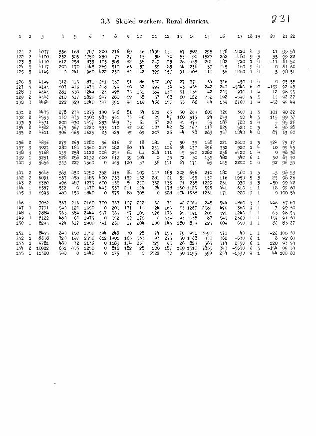
S13J1S!P iJfl}J sJI3poM PIIP1S

09 ool 1111 T 6 oÇÇ- tT4 66 4611 oÇ OL z249 o 66 4L1 O 011T O 0116 0lTT T 441

ti 66 i4i- Ç 9 oÇ9Ç- Ç14 498L oi4T 601 L9T 001 91 191 119 0 041T 401i 1Ç9 60T 1 11 6 011 T 9 o44 1114 496 i9 9 Ç6 ÇÇ 091 1101 Ç8TI o 9Çi L o9s T8L6 ÇÇj

09 16 9 T 9 0Ç9- 19Ç 041 990T o4 Ll Ç6 ÇÇÇ Ç9 10111 119 94Ç1 L61 olL 9499 T 14T 09 cOT 91 I T 011 oL4 o61Ç 146 6L ÇÇ 11L 9 OL 91 t16Ç o4LI 001 0111 44t9 T 141

Ll Ç9 98 T T 049 609 411 i8 091 1I 001 1101 LI 091 T6 0061 L19 i6 4ti T 041 09 16 6T 1 T 09Ç1 Çi4 L9 949 46 icÇ O 9L1 19 ÇÇ o 4L61 09 0911 1119 T 6111

Ç4 96 49 T T OI11T T6 901 161 46 9L1 914 401 L9 494 L44 ffjll t19Ç 96 1-199L T 8111

09 66 L T 6 o9Ç 9611 T9Ç L9i 44 49T tl 91 ILT Çol 0 0491 011 oic TLLL T L11T

09 L9 91111 T Ç 098- tjI4 41I1 1901 111 IL 04 Loi L9L ooL 0911 911 L9Ç 190L T 9111

i4 001 0 T 6 o ILT 1911 9941 f101 81Ç o o4 4L4 0 01191 041 o Ç669 T 41I 09 66 91 1 T 019 lIlli 464 4111 091 9L1 tl filT Ill LÇ4 4t1t1 oLlT o l44 L849 T 11t11

66 04- 4 T o6 T91 6T ÇÇ1 IL ÇÇ g9Ç o4 i 4T 009 GL1T L91 961 0849 1 ÇflT

91 96 6 Ç 4 o46T 911 041 Ç411 14 T6 191 141 14T ÇÇ 0011 4911 81 LÇ9 T609 1 liT 4 96 Ç- Ç 1 096 081 OIl 949 101 Çp L91 6oT 18 9111 lÇÇ O4lT o4 Ç9Ç 919g 1 TIlT

ÇÇ 96 16 11 T 0011 491 Ç8 ILT L9 TIT 8Ç LÇ 011 911 O 094T l Ç4Ç 911 Ç 0111 04 49 0 T 9 oÇ 191 ÇÇ oÇ L ÇÇ o flOT 66 119 009 lÇTl 841 814 1414 T 6T 94 96 0 11 1 olfi- 8Çg 1811 o9Ç 4i ITT Ill 11 119 141 901 llTT 941 641 9914 Ç 8Ç1

Ç 66 01 i T 016 1ÇÇ 969 LT 1Ç 911 141 111 09 191 Lfll o9Çi 1181 091 1104 Ç LcT LI 6L tll4 Ç T 0191 Ill 991 6Ç oÇ L 191 81 1 9T9 94 0911 Ç9l 6Ll 949fl 1 9ÇT

09 Ç9 L9 0 11 OliOT L9Ç Ç9l 9L flfj 91 Lol 69 6 4t1 Ç 4191 91 9O 1T91 1 9196 11 Ç T 014 dl LTT L9r 19 111 L91 001 li OTT 464 011T LÇ 4L9 19411 1 t1ÇT

91 46 6 fi T cOL L91 Ç4 iLl 1 Ol L9 19 4L 6tt ÇÇ L411T oÇ 001 1L4 Ç ÇÇT

L 66 611 Ç 11 OT Ç111 Ill 4TÇ 091 LI dl 911 9L 19Ç 496 0041 ÇL 091 T o6 101 Ç T 004 ol 009 191 04 49 TOT i 19 911 061 dLlI fiLl 8L1 dLt 1 TÇT

6 66 14- I 09L1 641 fl1ï 99 94 041 991 611 116 T6 L4 OtIOT 6l 111 19111 Ç oT Ll 16 di Ç 6 064- 161 ldL 111 09 89 LÇ 9Ç 69 091 Lil 0191 L14 oIl 91Ç11 T 611 44 96 TT t1 oL6 Çol lfl 9Çi 14 0T 694 T4T dL 961 ÇTT 6flT1 ÇÇ 181 Ç1Ç11 Ç 811 i T6 641- 0 9 O1OÇ- 0fT 1111 9611 Ç1 64 666 19 09 66T 911 ÇLflT 9111 Lo9 Ç6T11 Ç L1T

44 46 0 11 T 04- 914 119 ILÇ Ll LOT 109 99 14 ÇÇ 191 TL8 4TT lT 611111 Ç 911

id 96 Ç 11 T 0991 94 TIT 8011 16 L4T 66 TIlT 19 041 111 096 Ill 0 611111 Ç 4TT

09 19 0 1 6 091 411 64 941 11i1 Ç9 64T 6Ç 99 014 691 41111 OLT 001 LTT1 Ç ill 04 19 II- 11 T 0TL 191 ToT Ç911 81 Ç6 611 44 19 49Ç Çoi ÇÇ8 941 lT9 0111 Ç lT

1166 ÇÇ Ç 6 09fr 191 L14T 06 44 OL oÇ dl 12 LL 041 O4LT do 141 00111 1 111 tid 66 TT Ç 11 0101- 9LT 461 104 L9 1141 06111 99 69 911 001 L8L 991 9ÇÇ LLO1 T T1T

11 Il Ol 61 9T LT 91 4T 11 T lT TT OT 6 9 L 9 4 Ç 1 T

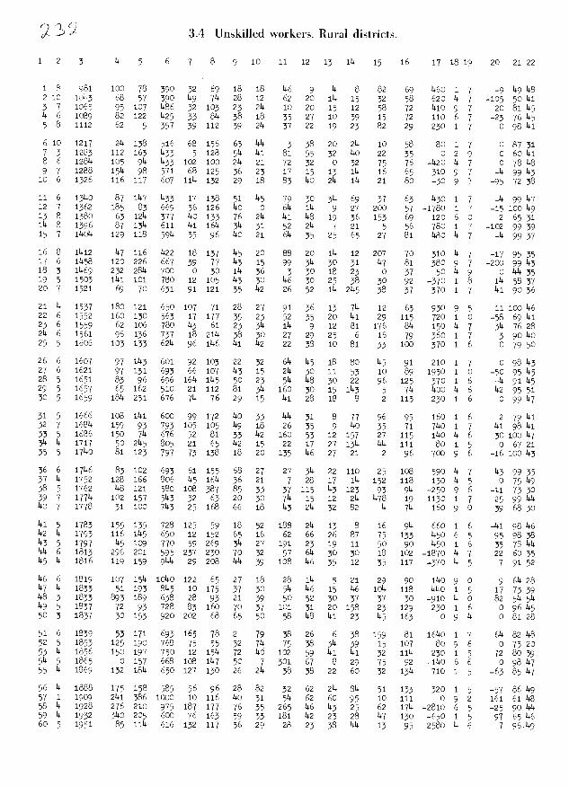
1 2 3

3.4 Unskilled workers. Rural districts.

14- 5 6 7 8 9 10 11 12 13 114 15 16 17 1819 20 2122

1 8 981 100 78 390 32 69 18 18 146 9 14 8 82 69 1460 1 7 -9 149 1482 10 10143 68 57 390 1#9 714 28 12 62 20 14 15 32 58 620 4 7 -105 50 1413 7 1065 95 107 1486 32 103 23 24 10 20 15 12 58 72 1410 9 7 20 81 14514 6 1089 82 122 1425 33 814 38 18 35 27 10 39 15 72 110 6 7 -23 76 1455 8 1112 62 5 357 39 112 39 214 37 22 19 23 82 29 230 1 7 0 98 141

6 10 1217 214 138 516 68 156 63 1414 3 38 20 214 10 58 80 1 7 0 87317 3 1283 112 163 433 5 128 514 14i 81 55 32 140 22 35 0 2 9 0 601418 6 12814 105 914 433 102 100 214 21 72 32 0 32 75 76 1420 14 7 0 78 1489 7 1288 1514 98 571 68 125 36 23 17 15 13 114 16 65 310 9 7 _14 9943106 1326 116117 6071114132 2918 83140214114 21 80 -3097 -957238

ii 6 13140 87 1147 1433 17 138 51 145 79 30 314 69 37 63 430 1 7 .14 99 14712 7 1362 185 83 669 36 126 140 0 614 114 9 27 200 57 -1780 1 7 -15 10014913 8 1380 63 1214 377 14o 133 76 214 141 148 19 36 153 69 120 6 0 2 65 31i14-8 1396 8713146111411614 314 31 52214 721 5 56 78017 -102993915 7 114014 129 118 5914 35 96 140 21 614 35 25 65 27 81 1480 14 7 14 99 37

16811412 14711614221813714520 882011412207 70 310147 -17953517 6 11458 120 226 667 39 77 143 15 99 314 30 31 147 81 380 9 7 -200 9914318 3 11469 232 2814 700 0 30 114 36 3 30 18 23 0 37 50 14 9 0 1414 3519 5 1503 1141 101 780 12 105 143 30 146 30 25 38 30 92 -370 1 8 114 58 3720 7 1521 69 70 631 91 121 35 142 26 52 114 2145 38 37 370 1 7 141 9036

21 14 1537 180 121 650 107 71 28 27 91 36 13 714 12 63 930 9 5 11 10014622 6 1552 160 130 563 17 177 35 23 52 35 20 141 29 115 720 1 0 -58 69 141236 1559 621067801436123314 114 91281176 814 150147 3147628214 6 1561 96 136 737 18 2114 38 30 27 29 25 6 16 79 360 1 7 3 9014025 5 1606 103 133 6214 96 1146 141 142 22 38 10 81 33 100 370 1 6 0 79 50

26 6 1607 97 1143 601 92 103 22 32 614 145 18 oo 145 91 210 1 7 0 9814327 6 1621 97 131 693 66 107 143 15 214 30 11 53 10 89 1930 1 0 -50 9514528 5 1651 83 96 696 1614 1145 50 23 514 148 30 22 96 125 370 1 6 -14 91145295 1657 65162510211128131416030151143 5 714 1400146 142955130 5 1659 1814 231 676 714 76 29 15 141 28 18 8 2 113 230 1 6 0 99147

31 5 1666 108 1141 600 99 172 140 33 144 31 8 77 96 95 160 1 6 2 79 14i32 7 16814 159 93 793 105 105 149 18 26 35 9 140 35 71 7140 1 7 141 98 14133 5 1686 150 714 676 52 81 33 142 160 53 12 157 27 115 1140 14 6 30 100 147314 4 1717 50 2145 805 21 65 142 15 22 17 27 1314 1414 111 80 1 5 0 67 2135 5 17140 81 123 797 73 138 18 20 135 146 27 21 2 96 700 9 6 -16 100143

36 6 17146 83 102 693 61 155 68 27 27 314 22 110 25 108 590 14 7 143 993537 4 1752 128 166 806 145 1614 36 21 7 28 17 114 152 118 130 14 5 0 75 14938 5 1762 148 121 580 108 387 85 33 37 115 143 123 93 914 -250 9 6 -11 73 3039 7 17714 102 157 5143 32 63 20 30 714 15 12 214 1478 19 1130 1 7 25 99 144140 7 1778 31 100 7143 25 168 66 18 143 214 32 82 14 714 160 9 0 39 68 30

141 5 1783 155 135 728 125 59 18 52 188 214 13 8 16 914 660 1 6 -141 98 146142 14 1793 116 1145 650 12 152 65 16 62 66 26 87 75 133 14o 6 5 95 98 38143 5 1797 14 109 770 59 269 314 27 191 23 19 11 50 90 14o 1 6 35 781414144 6 1813 296 201 595 237 230 70 32 57 614 30 30 18 102 -1870 14 7 22 60 35145141816 11915991414292081414391081463512 35117-370145 79152146 6 1819 107 1514 10140 122 65 27 18 28 114 5 21 29 90 1140 9 0 9 61428147 14 1833 51 193 8145 10 175 37 30 514 146 15 146 1014 118 1140 1 5 17 73 39148 3 1833 893 189 638 28 93 21 39 50 52 30 37 37 30 -910 14 0 82 514 514

149 5 1837 72 93 728 83 160 70 37 101 31 20 158 23 129 230 1 6 0 9614550 3 1837 30 153 920 202 68 65 50 58 148 141 23 145 163 0 9 14 0 81 28

51 6 1839 53 171 693 165 78 2 79 38 26 6 38 159 81 16140 1 7 614 82 14852 5 1853 125 190 768 75 55 32 714 75 38 314 39 15 107 80 9 6 0 73 2053 14 1856 150 197 750 12 i14 72 1414 102 59 141 141 32 111k 230 1 5 72 8039514 5 1865 0 157 668 108 1147 50 7 301 67 8 29 75 92 -1140 6 6 0 9814755 14 1869 132 1814 650 127 130 26 214 38 38 22 60 32 1314 710 1 5 -63 85147

56 14 1888 175 158 585 56 96 28 82 32 62 214 814 51 133 320 1 5 -57 8614957 1 1909 2141 386 1000 10 116 140 31 514 62 60 95 10 111 0 9 2 161 61 14858 14 1928 276 210 975 187 177 76 35 265 146 143 25 62 1714 -2810 6 5 -25 90141459 14 1932 3140 205 600 76 163 59 33 181 142 23 28 147 130 -650 1 5 97 65 14660 5 1951 85 1114 616 132 117 36 29 28 23 38 114 13 95 2580 14 6 7 96149

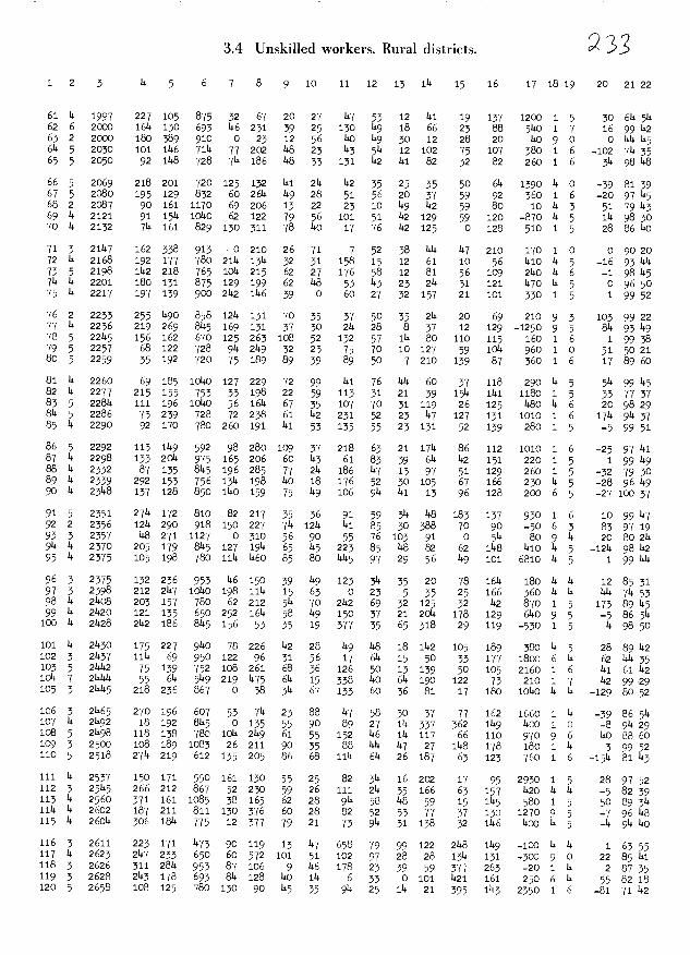
1 2 3

3.4 Unskilled workers. Rural districts.

14 5 6 7 8 9 10 11 12 13 114 15 16 17 1.819

61111997 22710587532672027 147 5312 l4 19 137 12001562 6 2000 1614 130 693 116 231. 39 25 1.30 149 18 66 23 88 5110 1 763 2 2000 180 389 910 0 23 12 56 140 149 30 12 28 20 140 9 0614 5 2030 101 1.146 7114 77 202 148 23 143 514 12 102 75 107 380 1 665 5 2050 92 1118 728 714 186 118 33 131 142 141 82 32 82 260 1 6

66 5 2069 218 201. 720 125 1.32 l4 214 142 35 25 35 50 614 1390 14 067 5 2080 195 129 832 60 2611 119 28 51 56 20 37 59 92 360 1 6682 2087 901611170692061322 2310119112 59 80 1011369 14 2121 91 1511 10110 62 122 79 56 101 51 142 129 59 120 -870 14 570 14 2132 711 161 829 130 311 78 140 17 76 142 125 0 128 510 1 5

71 3 21117 162 338 913 0 210 26 71 7 52 38 144 147 210 170 1 072 14 2168 192 177 780 2111 1311 32 31 158 15 12 61 10 56 1110 14 573 5 2198 1.142 218 765 1014 215 62 27 176 58 12 81 56 109 2110 14 6711112201 18013187512919962 148 5311323211 31.121 117011575112217 1971399002112111639 0 602732157 21101 3301576 2 2233 255 1190 858 1214 131 70 35 37 50 35 214 20 69 210 9 377 14 2236 219 269 8115 169 131 37 30 214 28 8 37 12 129 -1250 9 578 5 22115 156 162 670 125 263 108 52 132 57 114 80 110 115 160 1 679 5 2257 68 122 728 914 2149 32 23 75 70 10 127 59 1014 960 1 0805 2259 35192720751898939 8950 7210 139 87 3601681112260 69185101101272297299 1117614460 37118 29011582 14 2277 215 155 753 33 198 22 59 113 31 21 39 1514 1141 1180 1 583 5 22814 111 196 10140 56 1611 67 35 107 70 31 119 26 125 1480 11 6814 5 2286 73 239 728 72 238 61 142 231 52 23 147 127 131 1010 1 685 14 2290 92 170 780 260 191 141 53 135 55 23 131 52 139 280 1 5

86 5 2292 113 1119 592 98 280 109 37 218 63 21 1711 86 112 1010 1 687 14 2298 133 2014 975 165 206 60 143 61 83 39 614 142 151 220 1 588112332 871358115196285772111861171397 51129 2601589 14 2339 292 153 756 1311 198 14o 18 176 52 30 105 67 166 230 14 590 14 23118 137 128 850 1140 159 75 1 106 914 141 13 96 128 200 6 5

91 5 2351 2711 172 810 82 217 35 36 91 59 314 148 183 137 930 1 692 2 2356 1211 290 918 150 227 714 1214 14i 85 30 388 70 90 -50 6 393 3 2357 148 271 1127 0 310 56 90 55 76 103 91 0 514 80 9 14

914 14 2370 205 179 8145 127 1911 65 115 223 85 148 82 62 1148 1410 14 595 14 2375 105 198 780 1114 1160 85 80 1445 97 29 56 119 101 6810 14 5

963 2375 132236953116150391191233113520 781611 180111197 3 2398 212 2117 10140 198 ii11 15 63 0 23 5 35 25 166 360 14 14

98 14 21408 203 157 780 62 212 514 70 2112 69 32 125 32 112 870 1 599 14 21420 121 135 650 252 1614 58 119 150 37 21 2014 178 129 6110 9 5

100 14 21428 2142 186 8145 156 53 35 19 377 35 65 318 29 119 -530 1 5

101 14 21430 175 227 9140 78 226 142 28 119 148 18 1142 105 189 380 14 5102 3 21137 1114 69 950 122 96 31 56 17 614 15 50 33 177 1800 6 11

103 5 21442 75 139 752 108 261 68 36 126 50 13 139 50 105 2160 1 61011 7 214144 55 611 5149 219 1475 614 15 338 140 614 190 122 73 210 1 7105 3 21445 218 236 867 0 38 314 67 133 60 36 81 17 180 10140 14 14

106 3 21465 270 196 607 53 714 23 88 147 58 30 37 77 162 1660 1 14

107 14 21192 18 192 8145 0 135 55 90 89 27 i14 337 562 1149 1100 1 0108 5 21498 118 138 780 1011 2149 6i 55 152 116 i14 117 66 110 970 9 6109 3 2500 108 189 1083 26 211 90 35 88 144 117 27 1148 178 180 1 14

110 5 2518 2714 219 612 135 205 86 68 i111 614 26 187 6 123 760 1 6

iii 14 2537 150 171 550 161 130 55 25 82 314 16 202 17 95 2930 1 5112 3 25145 266 212 867 52 230 59 26 111 214 35 166 63 157 1420 14 14

113 14 2560 371 161 1085 38 165 62 28 914 58 148 59 15 1145 8o 1 51111 14 2602 187 211 811 130 376 60 28 82 52 53 77 37 130 1270 9 5115 14 26044 306 1844 775 12 377 79 21 73 914 31 138 32 1146 1400 11 5

116 3 2611 223 171 1473 90 119 13 147 658 79 99 122 2148 1449 -100 11 11

117 14 2623 2147 233 650 60 572 101 51 102 97 28 28 i314 131 -300 9 0118 3 2626 311 2814 953 87 106 9 146 178 23 39 59 377 263 -20 1 1

1193 2628 2143178693814128140114 633 01011421161 250614120 5 2658 108 125 780 130 90 145 35 914 25 114 21 395 1143 2350 1 6

2 3

20 2122

3061451416 99 1420 1414 145

-102 714 35314 98 118

-39 81 39-20 97 1455179113114 98 3028 86 140

0 90 20-16 93 144-1 98 145096501 9952

103 99 22814 93 149

1 99 3851 5021.1789605149914533 77 3720 98 29

1711 914 37-5 99 51

-25 971411 99 149

-327930-28 96 149-27 100 37

10 9914783 97 1920 80211

_1214 98 1121 99 144

128531144 714 53

173 89 145-5 86 514

14 98 50

28 89 14262 1414 35111 61 142112 99 .29

-129 80 52

-39 86 514-8 944 29140 88 60

3 99 52-1514 81143

28 97 52-5 82 3950 89 314-7 96118_14 914 140

1 63 5522 85 141

2 87 35558218

-81 71 112

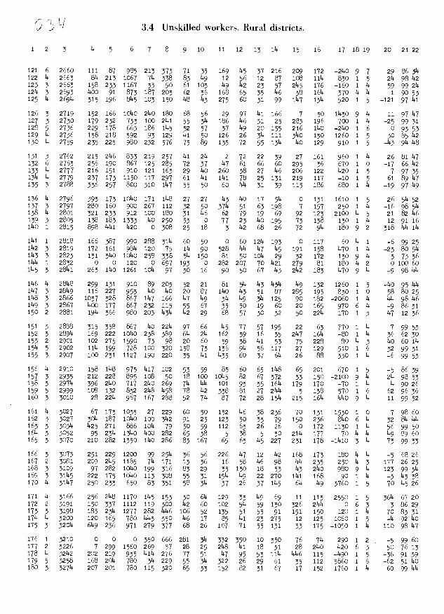
3.4 Unskilled workers. Rural districts.

114112818 16638799028831146050 0601214193 0117 60141 -699251142 3 2819 172 161 9814 120 75 114 90 528 t4 147 145 191 158 1470 1 14 -23 80 5141143 3 2823 131 3140 10140 258 338 514 150 81 50 1014 29 32 172 130 9 14 3 73 361114 1 2832 0 0 120 0 697 193 0 282 207 70 1421 279 81 180 14 2 0 100 601145 3 28141 263 1140 1261 1014 97 30 16 90 50 67 143 2142 183 1470 9 14 -9 98144

1146 14 28148 299 131 910 89 203 52 21 81 514 143 14314 149 132 1260 1 5 -140 95 1441147 3 28149 116 227 953 140 14c 20 87 1140 143 51 87 285 195 830 1 0 58 80 251148 3 2866 1037 328 867 1147 166 147 149 314 149 314 125 90 182 -2060 1 14 144 98 1461149 3 2867 1400 177 867 232 115 55 67 35 50 19 60 20 165 970 6 14 -9 8631150 2 2881 1914 366 980 203 14314 142 29 68 57 30 32 50 2214 170 1 3 147 12 36

151 3 2888 315 358 867 140 2214 97 66 145 77 57 195 22 63 770 1 14 7 99 53152 3 28914 169 222 10140 238 389 614 214 162 39 16 35 2147 1614 -80 1 14 36 62 30153 2 2901 102 275 1590 73 98 20 60 59 38 141 53 75 228 80 14 140 60 1141514 5 2902 1114 199 728 100 320 158 73 136 914 56 117 27 129 510 1 6 32 9931155 3 2907 100 231 1127 190 220 35 141 14 60 37 614 26 88 330 1 14 -6 99 53

156 14 2910 158 1148 975 1417 102 53 59 85 60 65 1148 65 201 670 1 5 -5 86 39157 3 2935 212 228 895 108 50 18 100 104-45 82 67 372 33 150 -2100 9 14 214 98 53158 3 29714 396 2140 717 2140 269 714 1414 101 93 35 1614 179 170 -70 1 14 14 9026159 5 2999 108 132 832 2148 1458 78 142 338 81 27 21414 5 138 570 1 6 62 96 36160 3 3010 28 2214 967 167 288 52 714 87 72 28 1514 215 1614 1440 9 14 11 99 52

161 14 3027 67 173 1035 27 229 60 50 152 146 38 236 70 131 1530 1 0 7 9860162 3 3027 3014 187 1O4C 100 3142 91 25 123 50 33 79 150 236 8140 6 14 32 814 1i4163 3 30314 1425 271 886 1014 79 50 59 112 6 26 26 0 172 1130 1 14 56 99 501614 3 3052 95 2314 i314o 1400 282 65 38 5 38 5 30 2114 177 70 14 14 149 89 60165 3 3070 210 282 1350 1140 286 83 167 65 63 145 227 231 178 -11410 3 14 73 9933

166 3 3073 251 229 1200 99 2514 36 56 226 147 12 142 168 173 180 14 14 -5 682616723081 209214511857141711336 165814698 144235 250143 1772625168 3 3109 97 282 10140 199 316 83 29 35 130 18 5 143 2140 980 9 14 123 99 314169 3 31145 222 175 10140 113 308 55 31 1514 149 22 270 1141 168 90 1 14 -3 14 38170 14 31147 250 233 650 8 351 58 314 37 26 37 1145 614 149 3760 1 5 70 14526

171 14 3166 256 2148 1170 1145 153 30 614 129 33 149 69 11 113 2550 1 5 3614 67 20172 2 3191 150 337 1112 119 300 142 60 102 514 59 130 326 2144 0 6 3 3 8629173 3 3198 185 2314 1277 282 1446 106 52 135 51 55 91 151 150 120 1 14 70 83 311714 14 3203 120 165 780 4-443 350 146 17 85 141 23 275 12 125 1060 1 5 _14 92 140175 3 32014 6149 236 971 279 377 68 26 107 71 55 131 33 175 -1050 1 14 110 98147

176 1 3210 0 0 0 350 666 281 314 332 350 10 350 76 714 290 1 2 -5 99 60177 2 3226 7 299 1560 269 57 28 25 2148 141 18 31 28 2140 1420 6 3 50 76 13178 L1 32112 202 219 935 14114 276 77 51 147 95 53 1114 1146 115 -4-490 1 5 -36 91 39179 5 3258 168 204-4 780 314 229 55 314 322 26 29 61 35 112 5860 1 6 -62 51 140180 3 32714 207 201 780 115 320 65 33 152 82 31 67 17 152 1760 1 14 60 991414

1 2 3 14 5 6 7 8 9 10 11 12 13 114 15 16 17 18 19 20 21 22

121 6 2660 111 87 985 213 373 71 35 169 145 37 216 209 172 -2140 9 7 29 86 314122 1 2963 84 215 1067 714 338 83 119 12 56 12 87 108 1114 830 1 5 214 98 42123 3 2663 158 233 1167 33 50 61 103 149 142 23 57 2145 176 -160 1 4 59 9921412143 2693 14009187318720362361686535146 381614 3701414 19053125 4 26914 315 196 814 103 150 148 143 275 60 31 99 1147 1314 520 1 5 -121 97 141

126 3 2719 152 166 10140 2140 180 68 56 29 97 41 166 7 50 11430 9 14 11 97147127 3 2730 179 232 733 100 2141 55 314 186 146 31 25 283 196 700 1 4 -25 99 31128 5 2736 229 178 663 186 1145 52 57 37 149 20 155 216 1140 -2140 1 6 0 93 53129 14 2736 158 218 592 93 129 141 50 126 26 314 111 3140 130 1260 1 5 30 85 42130 14 2759 235 225 980 232 576 75 89 135 72 55 1314 14o 129 910 1 5 -143 914 148

131 3 2762 215 2146 833 219 257 14i 214 2 72 22 39 27 161 960 1 14 26 81 147132 6 2763 256 190 867 125 285 72 37 147 61 66 60 295 36 670 1 0 -17 66142133 14 2777 216 151 910 121 163 29 140 260 38 27 146 206 122 1420 1 5 7 97 351314 14 2779 237 173 1150 117 297 61 141 1141 78 25 131 219 117 -10 1 5 61 89147135 3 2788 336 257 800 310 1147 55 50 60 144 31 39 115 186 680 1 14 -19 97 149

136 14 2796 393 173 10140 171 1148 27 27 14 140 17 514 0 131 1610 1 5 26 514 52137 3 2797 280 160 900 267 112 32 50 3714 51 63 198 7 157 250 1 14 -i6 98 514138 14 2801 321 233 912 100 180 31 146 62 79 19 69 92 123 2100 14 5 21 82 146139 3 2805 138 183 1333 140 250 53 0 77 23 14o 195 73 138 130 1 14 12 91 161140 1 2815 898 14141 1420 0 308 25 18 3 142 68 26 72 914 180 9 2 318 1414114

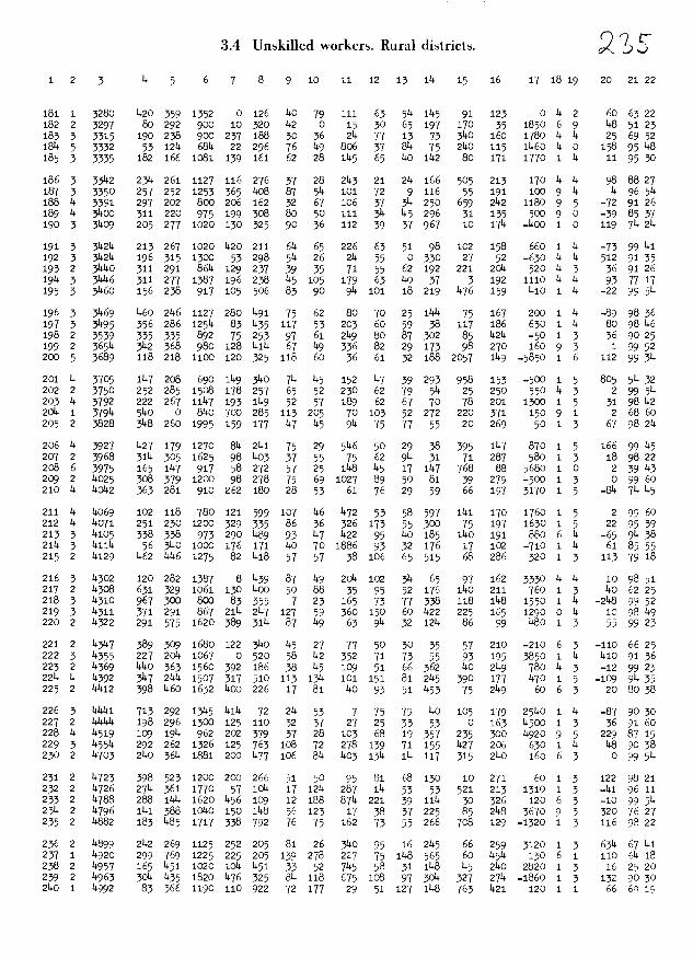
3.4 Unskilled workers. Rural districts.

1 2 3 14 5 6 7 8 9 10 11 12 13 114 15 16 17 18 19 20 21 22

1811 3280 14203591352 012614079111635141145 91123 0142 606322182 2 3297 80 292 900 10 320 142 0 15 30 65 197 170 35 1850 6 9 148 51 23183 3 3315 190 238 900 237 188 30 36 24. 77 13 73 3140 160 1780 14 14. 25 69 521814 5 3332 53 124 6814 22 296 76 149 806 37 814 75 2140 115 11460 14 0 158 9514.9

185 3 3335 182 166 1081 139 161 62 28 145 65 40 114.2 80 171 1770 1 14. 11 95 30

186 3 33112 2314. 261 1127 116 276 37 28 214.3 21 214 166 505 213 170 14 14 98 88 271873 3350 257252125336514.0887 514 10172 9116 55191 100914 14.96514188 14 3391 297 202 800 206 162 32 67 106 37 314. 250 659 214.2 1180 9 5 -72 91 261891431400 3112209751993088050111314145296 31135 50090 -398537190 3 3409 205 277 1020 130 325 90 36 112 39 37 967 10 1714 -400 1 0 119 714 214

191 3 314214 213 267 1020 1420 211 614 65 226 63 51 98 102 158 660 1 14 -73 99 41192 3 314214 196 315 1300 53 298 514 26 214 55 0 330 27 52 -630 14 14 512 91 35193 2 34140 311 291 8614 129 237 39 35 71 55 62 192 221 2014 520 14 3 36 91 261914 3 31446 311 277 1387 196 238 145 105 179 63 40 37 3 192 1110 t4 14 93 77 17195 3 31460 156 238 917 105 506 83 90 914 101 18 219 476 159 14io 1 14 -22 99 514

196 3 31469 1460 2146 1127 280 491 75 62 80 70 25 1144 75 167 200 1 14 -89 98 36197 3 3495 356 286 12514 83 1435 117 53 203 60 59 38 117 186 630 1 14 80 98 146198 2 3539 335 335 892 75 253 97 61 2149 80 87 302 85 14214 -50 1 3 36 90 25199 2 36514 3142 368 980 128 14th 67 149 336 82 29 173 98 270 160 9 3 1 99 52200 5 3689 118 218 1100 120 325 118 60 36 61 32 188 2057 1149 -5850 1 6 112 99 314

201 14 3705 1147 208 690 1149 340 714 145 152 47 39 293 958 153 -.500 1 5 805 514 32202 2 3750 252 285 io8 178 257 65 52 230 62 79 514 25 250 550 14 3 2 99 514203 14 3792 222 267 1147 193 1149 52 57 189 62 67 70 78 201 1300 1 5 31 98 14220141 37914 5140 0 8140700285113205 70103 52272 220 371 15091 26860205 2 3828 3148 260 1995 159 177 47 45 914 75 77 55 20 269 50 1 3 67 98 214

206 14 3927 1427 179 1270 814 2141 75 29 546 50 29 38 395 1147 870 1 5 166 99 14207 2 3968 i14 305 1625 98 1403 37 55 75 62 914. 31 71 287 580 1 3 18 98 22208 6 3975 165 1147 917 58 272 57 25 114.8 145 17 1147 768 88 5680 1 0 2 39 143209214025 30837912009827875691027895081 39279-50013 09960210 4 140142 363 281 910 262 180 28 53 61 76 29 59 66 197 3170 1 5 -814 74145

211 14 14069 102 118 780 121 599 107 146 1472 53 58 597 1141 170 1760 1 5 2 99 60212 4 14071 251 230 1200 329 335 86 36 326 173 55 300 75 197 1630 1 5 22 95 39213 3 1410 338 338 973 290 1489 93 147 422 95 40 185 1140 191 880 6 14 -65 94 382114 3 41114 56 3140 1000 176 171 140 70 1886 93 32 176 17 102 -710 1 4 61 85 55215 2 14129 462 446 1275 82 1418 57 57 38 106 65 515 68 286 320 1 3 113 79 18

216 3 14302 120 282 1387 8 439 87 149 2014 102 34 65 97 162 3330 14 14 10 98 51217 2 14308 631 329 1061 130 1400 50 88 35 95 52 176 1140 211 760 1 3 14o 62 25218 3 14310 967 300 800 83 355 7 23 165 73 77 338 118 1148 1550 1 14 -2148 99 52219 3 14311 371 291 867 2114 247 127 59 360 150 60 1422 225 165 1290 0 14 10 98 49220 2 4322 291 575 1620 389 3114 87 149 63 914 32 1214 86 99 1480 1 3 55 99 23

221 2 143147 389 309 1680 122 340 145 27 77 50 30 35 57 210 -210 6 3 -110 66 25222 3 14355 227 2014 1067 0 520 58 142 352 71 73 55 93 195 3850 1 4 1410 91 36223 2 4369 1140 363 1560 392 186 38 145 109 51 66 362 140 2149 780 14 3 -12 99 23224 14 14392 347 2114 1507 317 510 113 1314 101 151 81 245 390 177 1470 1 5 -109 914 35225 2 14412 398 1460 1632 400 226 17 8i 140 93 51 453 75 2149 60 6 3 20 80 38

226 3 14441 713 292 1345 14114 72 24 53 7 75 79 14o 105 179 25140 1 14 -87 90 30227 2 1414144 198 296 1300 125 110 32 37 27 25 33 53 0 163 14500 1 3 36 91 60228 14 4519 109 194 962 202 379 37 28 103 68 19 357 235 300 14920 9 5 229 87 15229 3 45514 292 262 1326 125 763 108 72 278 139 71 155 1427 206 630 1 14 148 90 38230 2 14703 240 3614 1881 200 1477 106 814 1403 1314 i14 117 315 2140 160 6 3 0 99 514

231 2 14723 398 523 1200 200 266 51 50 95 81 68 130 10 271 60 1 3 122 9821232 2 4726 2714 361 1770 57 1014 17 1214 287 14 53 53 521 213 1310 1 3 _141 96 11233 2 4788 288 11414 1620 1456 109 12 188 874 221 39 1114 30 326 120 6 3 -10 99 54234 2 4796 1141 388 io14o 150 1148 56 123 17 38 37 225 85 248 3670 9 3 320 76 27235 2 4882 183 1485 1717 338 792 76 75 162 73 55 266 708 129 -1320 1 3 116 98 22

236 2 4899 2142 269 1125 252 205 81 26 3140 95 16 2145 66 259 3120 1 3 634 67 141237 1 4920 299 769 1225 225 205 139 278 227 75 1148 565 60 14514 130 6 1 110 614 18238 2 14957 165 1451 1020 1014. 451 33 52 745 58 31 148 145 2140 2820 1 3 16 25 20239 2 4963 304 435 1820 476 325 814 118 675 108 97 3014 327 2714 -1860 1 3 132 90 302140 1 4992 83 366 1190 110 922 72 177 29 51 127 148 763 1421 120 1 1 66 69 19

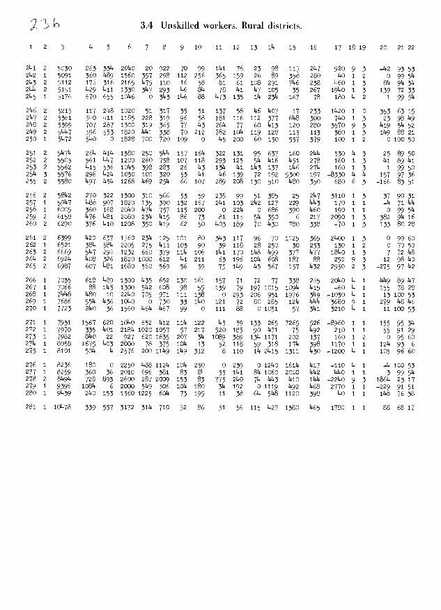
Li g9 T i o9L1 49t1 o96T L?t1 411 94 T6 99 oL 11T LT6 L44 644 9LIiOT T 19?

96 9L 9111 1 T Olj 966 0T 94 t19 96 TT 461 6L t109 0941 64T o 661i6 i og T4 T6 6æ- I T 0LL? 9911 611 6TT o 6T f 091 110T 906 6 000? 9 1190T 9666 1 6L LT 4? t1i c 6 O11?- ffiT 0T11 6i L 4LL 6g 64T 600? L9? 009? 669 9?L 11611g ? 9L?

66 6 T T 0t1l ?t111 000? 090T 119 TiT c4 t9 49 T96 969 010? 96 096 64g T LL? 64 OOT t1- 1 OTT LTI1 11T9T Ot??T 0 66? 0 0 1101 11?TT 8811 o4? 0 09T 96?9 I 9L?

09 96 401 T 11 C)0?T 0611 TI6T 4111? tIT OTT g ?16 611T 611T1 00? 9L4? 11 1104 1019 T 4L? 9 66 11?I T T OLTT 966 11LT gTÇ 64 8TT 4 61 11OT 4L6 9L 000 6o 4L9T 9608 1

09 46 0 ? T 09T L61 ?0? TLTT IIÇT 696 6901 11 Lo 4Ç91 0?9 L6 O19 ?96L T 6L 6? T6 44 1 T 01? ?611 4L TL11 06 49T o4 LT? L4 L4oi o?0T 1191? 1ot 4Ç6 0L6L I ?L

11 46 44T I T 0969- 9?4 49L 49 4T 64 411 ?T IITT ?T11 49 O1OT 09 L94T T46L I TL

64 OOT TT T 11 0T?6 TIiÇ L4 T4OT 0 99 ITT 0 66 L911 11911 0941 94 O* 6?LL i oL 911 811 6L? i 6 0996 1Tt111 11T 49 09 L IiI 011T 66 o6L o 01101 911 114g 999L i 69 64 COT 4T 1 11 060T 6t16 9L6T T46 90? 66? 0 96T ITT IL6 4oL 011?? OT 0911 9t1i1L 1 99? 9 9L 441 1 11 09- 4111 11601 4TOT L6T 6L 66T 44 86 909 ?t4 oo4i Ç11T 99 990L T L9?

Li 68 6t i 11 O11O 49? 966 LL ?L TL L4i T9T OT ?49 Ç6t1 oo4T 6911 9T9 4coL T 99

t1 L6 4)2- 6 o46 ?6t1 L4i L94 411 611T 6L 64 94 694 094 099T T Lo9 L969 49 011 96 ?T 4 6 o4 99 L9T 909 1101 96T 69 TT? T11 T9 000T O?9T 9?6 8011 11?69 ? 119e 811 L L 6 T 0118T LL11 LL6 6611 9111 OLT lIlT 90T 11TT 6L6 099 Ç1 96 L114 6999 69? 04 OL O T 06T 44 06 o4 9 9TT 66 06 60T TT11 4L? 4o 1i94 119f T49 T

09 66 0 6 T 0011? 496 4?TT OL 96 LIT 09 TOT 4?T 116? 0961 L69 0?11 6669 ? T9?

8 09 T OL- 96Ç o9L oÇt1 OL 69T Çot1 0 ?9 6111 o4 90T OI 9L o6?9 09? 9T 116 g6 Ç I o6oe LT? 9 o4 t14 ÇTI 19 6L 99 4T11 tÇ 09 1911 9L11 94T9 ? 6? tÇ 66 0 o6T 0911 066 999 0 hæ O OO 4TT LL tLt oo 99T 096 4009 1 8?

+111 TL r I T 0LT Çti 6? L?T ?j? 601 T11 L9T 4T o6 41 O9T Lo6 99i L116 T L2 T 06 L Ç 1 OTT6 L? 4 Ç9Ç 66 4c 6 6Ç 994 OT4 6T ?Ç oL ?118Ç 3 9

T 6g 99V Ç 9 089 046 0911 0T 04T 90? 69? LOT 99 t1? 69t1 99?T ct L611 0944 94 L6 L4 t oÇÇ- L6 0064 ?6T L 66i 911 111 Ç O?6 001 0601 t11 96 9L4 4 04 66 T Ç I 09T 11L? 911T L4T Ç11T T11 iT Çt 9 6 96Ç ÇtoT 964 4Tt ?944 TIl 68 111 4 1 09T 9)2 9T11 t1 4T 6? 9T1 LOT 9L 09 OOT Lt 194 4044 04 6g 4 4 t o4 111Z 09T L49 46 T6T ?6 t9T LT 1iliÇ o4 096T tTj t19 tL114 ? T

O OOT O I OoT 6L6 L4 OT 09 ooe o 6oT OL ooL 9?91 O 0i L11Ç I o T 99 6111 6 ogÇ TT 4TT 9?T 6TT 1OT gL ZT? OL 9Ç6 T111 O9i 64 96 Lt1i ? 611?

114 6T 6 6 oL6 09? O?T ÇTt1 09 LL Ii9 11 LL 94 6T6 OOÇT L9? L0L 66 3 9t? 61186 ? T OjL oo 8119 LL6 TT 9TT T9T 94 96 6Tc 9 49TT TTt Oi I9ÇÇ

I 69 Ç44 o I 011T 6 LT Lo11 911 94 L4T T Ç LT4 T4 0?OI 9i LTT ÇT? 9t?

t66T ?O91 9L L9T Z11T ÇÇTÇLII 9 911T61140 91lOT49OL9 9LT T11? 66 L 66T T 0116T L9 ÇÇ 4oT L11 Tj 9L t 9 L116 o46i ThI 6j Ti i6 116 9 4 1 09t 9? 9jL T6 OT 19 19 9 91 0Th Lj 49 91Ç 9LT ?IT 114 66 o ? I Oj 09? g4Ç 68 9? 6T 49Ç 9 T1 86? L4 094T 096 T604 T 44 66 - 6 o?6 L? 4TT 96 9L T111 66 OL ?6 0? Ot1O I1ÇÇ Ç93 o6o ? Tt?

T O 6T 91 LI 91 I 11T 61 ?T TT OT 6 9 L 9 T

SZLflSip 1Jfl}J SJJOM P1IP1f1 V

3.5 Agricultural workers. Rural districts. 2 R1 2 5 4 5 6 7 8 9 10 11 12 13 14 15 16 17 18 19 20 21 22

1 10 872 7 65 522 23 88 29 314 36 34 7 5 14 51 150 1 7 20 60 412 9 907 514 80 1404 15 82 53 16 140 21 5 6 42 75 5140 6 7 -119 53 1455 9 918 97 81 1404 7 148 34 24 51 17 5 17 194 18 420 5 7 0 98 814 9 967 130 88 549 19 20 22 26 7 15 0 6 91 55 220 2 7 21 75 575 5 985 37 1144 572 97 6 13 50 3 24 0 9 17 141 -160 5 6 -5 76 44

6 9 1000 28 91 289 21 85 50 28 414 19 8 90 22 143 220 14 7 1 99 417 5 1009 98 77 2140 24 71 34 51 53 42 0 50 73 83 250 1 6 67 67368 14 1075 18 108 440 156 85 26 27 5 50 14 86 10 5 70 14 5 -10 95 519 6 1097 170 105 435 15 58 18 22 6 10 17 50 24 26 710 1 7 22 55 40

10 2 1124 547 552 845 52 53 26 157 157 36 35 52 430 35 -3960 3 0 320 74 52

11 6 1127 191 129 14ss 3 26 13 47 100 39 15 9 5 92 520 1 7 0 76 4512 5 1142 73 106 624 144 25 14 15 17 15 10 6 10 75 0 14 6 ..5o 63 28156 1155 558452890572550 29412128 17 96 19017 34675514 6 1170 100 171 433 7 31 i14 57 41 22 56 15 62 76 260 1 7 -14 55 4815 7 1262 69 4 557 37 21 45 57 17 25 14 128 14 714 590 14 7 0 84 60

16 5 1288 96 102 510 87 91 51 21 25 59 20 63 40 1i4 80 9 6 0 74 42177 1295 77100624741515528 62201731 50 72-90047 -107232182 1317 2502877804382 757 22124129181 66-18504 5 517051419 6 1383 116 110 533 40 70 14 27 3 50 19 10 226 80 370 1 7 -8 98 5120 4 1401 0 90 s85 61 50 30 32 597 57 20 159 60 37 -630 1 5 9 100 60

21 5 1405 103 151 696 5 76 26 35 68 41 20 11 26 91 60 4 6 -14 65 4922 5 1408 117 214 552 55 62 50 44 70 26 8 38 21 102 120 1 6 17 52 4525 6 1415 0 162 6o 44 27 17 38 74 29 5 50 22 76 220 9 7 -7 99 4824 5 14114 212 252 515 76 i4 22 49 28 54 16 57 42 100 -420 1 6 -5 28 4255 1420 4810178042581425 26515250 19 95 8046 0712226 5 1477 118 1140 852 209 125 49 29 15 29 26 35 18 86 490 1 6 0 98 4727 5 1479 67 95 596 129 69 57 15 167 27 16 59 0 120 -2420 1 6 20 994528 2 1482 13 86 910 56 27 19 11 0 15 21 50 61 74 -150 4 3 12 51 5229 5 1488 914 124 572 52 55 24 16 42 33 12 61 10 97 470 9 6 0 98 4730 5 1515 80 1314 624 50 100 31 56 84 51 11 19 20 97 270 1 6 0 98 52

51 4 1545 81 175 910 50 169 56 45 84 45 54 65 70 95 -1580 2 5 80 76 14325 1575 012892811 6 5117 42216064 0 58 16036 0985155 6 1622 42 88 7814 117 150 48 56 41 50 26 52 70 56 -160 6 0 -15 965834 14 1630 63 166 780 80 164 12 51 105 38 7 12 57 116 60 4 5 -2 755355 6 1655 88 io4 695 131 98 42 514 74 42 26 66 11 78 560 1 7 -6 98 60

64 1682 127215 390 0136564717028 816 67 36154045 -4875537 6 1684 89 145 600 52 174 51 59 66 45 114 78 55 78 100 1 7 -36 75 38385 1686 173182867159731874 3281189 7169-65064 0945559 5 1688 60 166 6214 187 72 53 4 84 50 28 154 51 85 120 6 6 0 65 5040 4 1691 152 1814 530 0 2514 47 45 135 40 22 127 37 117 _40 1 5 42 97 54

4141709 186145650771051537 70391653 82144 35045 1975042 14 1714 116 150 1416 12 296 41 37 170 52 25 55 51 116 850 1 5 18 994643 2 1734 106 95 10140 59 15 15 70 5 10 56 22 0 196 160 14 3 50 50 2444 5 1745 145 64 520 58 512 65 6 79 26 20 25 56 105 620 1 6 11 96 4i4 5 1771 154 104 458 32 158 68 31 507 4o 20 151 24 31 570 1 6 -15 9948

46 5 1782 171 97 728 86 65 25 58 19 4 18 64 26 124 410 9 6 -55 7514t47 3 1799 2146 203 800 56 86 25 21 4 20 35 69 150 185 -400 14 4 L 62 604841800 123148845511556541 42642753 17110 13015 098514951808 18281468 016576362025218157141109-24046 355714150 5 1825 8 47 624 84 102 44 19 15 46 23 59 225 89 650 1 6 4 76 42

51418314 1551506251006233 9194312457 82 140 50095 -3975352 5 1861 87 162 7314 81 179 31 20 21 17 146 152 146 76 150 1 6 -3 98 5153 4 1883 1 i1 775 87 258 45 19 98 5 147 70 90 88 490 14 5 14 98 146514 4 1912 96 106 910 125 88 39 20 13 15 22 118 52 139 -90 14 5 328 84414553 1919 5517272816035 4 743375220214 30 56 160144 15995156141920 271826501321052175 80613011 42144123055 195054573 1930 215161867408425012 7255550 18118-540614 705852

14 19149 400 165 650 17 161 28 3 63 50 15 35 33 107 2720 1 5 0 98 4559 14 1968 156 187 910 96 62 35 22 172 36 62 40 36 122 100 9 5 0 773260 4 1992 223 182 1072 80 100 49 18 59 1444 46 46 14o 135 650 9 5 -3 84 42

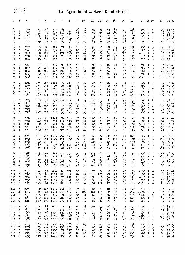
20 21 22

-20 831438 90 52

15 86119-29938326752

119 47 14132 86 42138530

1 87 511-19918

3 90 148_3 975166 76 26

0 99 531978742

09831-28938814 11611534 33 113-8 49 30

1 98 4170 93 42-9 100 5135 69 44114 50 43

496441346127

88142408 100131600543124737165352752 40130311095 668741

119 2 30811 2114 307 10110 9 99 28 43 190 32 40 102 43 247 440 1 3 148 711 23120 2 3095 210 261 1423 284 71 40 6 17 4 66 66 235 256 120 6 3 0 74141

89 14 2414 232 136 1040 41 186 48 74 87 82 23 86 76 122 810 14 5 -58 783590 14 21444 150 187 861 323 129 24 44 97 4 41 37 186 114 320 1 5 -4 92 53

91 3 21490 133 193 1105 200 128 31 25 61 30 42 173 123 205 120 1 14 0 87 4592 14 2556 192 1144 1105 1144 180 30 36 105 41 1i4 114 354 30 -220 9 5 147 54 2093 3 2561 320 191 1127 33 914 25 25 108 67 12 77 45 160 180 6 14 0 99 3594 1 2563 180 13 549 161 266 117 158 33 19 614 159 1714 81 230 3 1 36 956095 2 2568 213 333 780 25 120 71 18 3 15 33 70 72 92 830 9 3 143 99 60

96 6 2582 233 1514 818 102 372 90 33 315 82 17 140 118 56 -1490 14 7 -152 96 3797 5 2585 167 142 936 41 149 68 25 1446 36 26 22 288 107 520 1 6 -83 87 4098 3 2587 219 195 1103 105 191 51 43 105 29 34 108 53 169 5110 1 14 6 92 4599 2 2627 220 252 1040 475 62 25 0 75 32 42 40 15 85 550 9 3 0 60 32

100 14 2636 19 170 765 175 338 57 38 261 106 4i 368 97 92 40 14 5 48 84 28

101 5 2638 142 155 864 45 221 50 18 72 32 0 32 43 53 2660 1 0 73 5641102 3 2645 100 146 1253 101 102 24 69 111 105 48 192 52 133 60 1 14 1 90 25103 3 2654 268 231 1127 73 219 41 62 138 60 36 67 37 171 -110 1 14 1 75 114104 1 2656 80 250 1105 138 142 20 56 81 69 50 711 55 121 770 1 5 52 99 27105 3 2685 178 1014 1387 106 501 63 67 554 121 17 159 85 169 -1650 9 14 20 97 36

1063 2694 90223133315175 738 82781012 23170 380411 -38152107 2 2711 378 362 1560 215 462 61 100 464 103 72 177 190 258 -3110 14 3 97 9921108 3 2719 198 252 953 94 142 52 61 69 8 36 98 24 191 11440 14 14 37 54 24109 3 2746 140 213 1127 226 192 17 52 71 81 32 23 41 166 800 1 14 41 97 52110 2 2825 180 259 1170 276 248 6o 37 88 42 25 58 45 266 120 6 3 0 98 48

111428314 45889547633260282045736130 92173103045 88335112 2 2871 166 26 845 373 352 50 22 1 87 37 42 1149 214 360 1 3 63 89 221132 2885 2025815602311205337 19748577 60 914 18023 099111114 14 29114 2 170 145o 87 388 71 614 98 81 33 45 134 59 1380 9 5 116 98 38115 2 2987 210 293 1300 190 153 29 59 176 56 30 35 799 243 -1620 2 3 42 72 20

1163 3017 16020713001333887047 79954567100174 26094 37435117 2 3024 135 1414 1139 250 506 58 28 6o 41 36 514 59 96 80 14 3 670 61 2411823080 156111113002732763124 69253415 24165 44043 389955

3.5 Agricultural workers. Rural districts.

1 2 3 14 5 6 7 8 9 10 11 12 13 14 15 16 17 18 19

61 3 1995 ill 186 867 67 164 28 18 81 41 33 45 27 154 350 14 14

62 5 1999 82 133 819 119 262 32 35 69 43 12 1149 6 25 120 3 0634 2000 105151 765 502022720 5521550 32 140 790156144 2017 0114787515613911878 9636 16104 35124 22015653 2020 149119104095943363 11511238118 76 55 606466 2 2026 80 168 825 77 78 21 26 156 30 48 25 33 254 200 1 367 5 2041 148 98 759 118 153 40 17 130 33 37 111 38 1014 11140 1 668142066 50181 650171223 12 12 119 314 3660220 87 -8809569 3 2094 100 191 953 76 105 25 27 33 35 22 90 21 173 0 1 14

703 2102 115218 907 01233331 71391028 52107 38011471 7 2103 7 76 929 96 461 63 16 88 52 19 61 67 45 250 1 572 11 2115 25 128 875 71 195 57 75 189 69 211 66 111 101 260 3 573 2 2116 311 211 800 100 86 31 31 1514 36 56 16 12 80 20 6 374 3 2134 0 175 833 1148 85 115 30 80 60 14 1611 42 51 810 1 14

75112138 7511378053112117111 1930 620 45 14262095763 2181 155188121390211111327 273916 0 3 46 i2011773 2193 2331146600261163637114935621482147173 260111478 3 2205 17 175 935 17 111 16 19 0 19 13 515 7 193 140 2 079 14 2239 307 181 325 52 167 92 57 143 55 18 26 316 1113 900 j 580 2 2240 180 225 805 132 191 44 62 231 714 25 35 100 253 -390 9 3

81 3 2273 240 131 693 121 206 28 33 129 27 24 11 139 175 160 6 14

82 14 2276 219 232 650 0 120 43 10 107 81 25 1140 18 180 1180 1 583 3 2296 294 200 867 0 159 48 24 11 39 25 12 10 167 1250 9 14

84 3 2305 181 341 693 59 398 127 10 2 30 57 28 6 190 430 14 085 2 2323 247 377 780 95 146 36 35 55 28 11 52 13 59 400 14 0

865 2392 781961040872033329163563197 36 71 65016872 2399 3423997501172104799 69272212136 68 12013

666çTToiloi9?TTTT Çi1T99??cL9LilT99?90?o9çilOT9T09T iLi6c-çt occTccT6i1oji1T?6gc699ç9L?L?T99Tl?9T900?66TL?6cToc cTiloilç-gcçcToc?T6c?9l?cg?9cooogccççgçLÇ9T gT ? cgççilOcT-T??g?6T609ill?9TL6?LoLilgoço?6TTocTT??LcT91j 66?T9hOT0ThL6?cLoL009TLgil9ccc6cgj1ç6TccT 9T0969ilTcoo?99ilc?T669c6LT6).ç9cho?ilo?6TcilTT6cc TccT 9h1 66LT-Tilot1L?cTO?occccc9?L9il?cTcg9?).ç9ç0?cgocgOTcTilcT 09 OOT OTTTOOT90To?T9L6 ocL?TO?co?TOTTo6LT9?TcTTocT6æcTccT09 Lil66TT?oL9-09?1jccTTLTc9Tch1Tgcï0cc000c?L ogcggiT?cTil? gL oc6oLoT?c?06OcTci99??c9gçoci1ocoO?T 099 o?6i1119i1?TcT

?11 c9ilLTTT06TTLL??Lc6il99691?LOL6L?T?6?gL?T99Til9Til9ilTocT9? TocT66oLgTcc?OcTT99çLç996igçco?9c?ocTTi1i1ÇhT9cgcil?6h11c? 96ccTo9c?9?il?T?T6coi gcLilc9il69LO?oocToLOL?Tcs?9ilT9ilL9?T?0?9ilcil?OTcil?c6?cç0çOTT6?ccOOToogc?ilsçccTLiii9? cc6hT9OT0T8çL6To?6o?9cLTil??99c?9?T096Lcil?ilToccilT9ilT

09 ?c O?T?O90Tc6T?6c9il?T090cc?cç6T669ogL9??119Lt1oÇs1Tchi c? c9gçciococ??TLcLoTcciliTcT0?96co9cOLTTcTc96T9L011?hilT9T L6TcçToilL60TTil9Tç?cT9cc?OilL?oil90?i1ccTcc?To?ilcoil?çilT09 99T90il96LLccTOh?9118OOT9OTT9?c?Til9cT6c??Lil911011T?hT09119hOTTço6??9??0TggcilLÇ9?699189 g6ccoilcThç6TccTohTTIIT

6i g6coTçoL699T?h69?6hT?TLilLc96?ilTO9T ???LO?TOOil?0hTL?ilT0h16Lc?110?TT?ocil?TL6Oilcgc9?oc?o?oT cc Toc?LLc?6cT91100TTçTOh1gc9??98Til?Tco?8ç09?LO?8TL6?Oil?699f9cTLT 669?çilo6i99oUT?T??c99o?611ilcTc?c?? cdTgiL9cT9ç? LT 9cL96diloccil?8L9TT?c96Ldi110Th?il9T09TOOilTT8çh9??9cç?9cTLi6coccTcx)c11t1?ocLTT?cic6LiloocT9Tccç000TL9ç9Lç??cc?ccT L99i1Togç0??c99ciiTcccccL99L09ilLTTod66ToiçcijdiL? i19çci06Til?ocTccilTL?ccLc9cT?9?LOI1OT110?6d?çgcç?ccT9cT9OTT11T0hcTiL?c?ilild9ocilL?Lcil?ç9cT?TLcTO9c6?cc?cT c? L8cTililo?Lcç?occ?8TiLc9TT?cc9c?TilLo66gic99?9?ccTcT

911?c1rcOOilT0?T9LOTL?6?686icoc?ilcLil090199T9111c9?ci1OcTL?986Tchog?99TLililLil99?9il9TcTTco9cicch6cc911?ç?6?T cc L9TT-ilT06?091c?T60Til?ilL99?090?Tciç ocL9g99cgc?oil?dç9?T8? 96L6çilO?hT?LcT6oTL?6cTcL9c?Tc?ToodiL??oc?c??c?L?TL? 96Tç09969cc6c61?OTTcTc9ilT?oçilT601109c6Tc?9?T

ilc96 ociloci?o??LTTT96ilcLL9cTilo6cildiLoi9ch?LTg9Td?c?T?c ?6cilTilT09-il9T99ilL?9L6c066?go??1161cT?T6cTT919?Tcçh?T gTL6oc9occ06c??cTL9L9ci?cil?il?cTocT000To?cLç???Tc?c?T çç 66oçil089??OcT61il9ccT?8cLicc8d0T61111?OTgTTç???Tc? 69?cooT-c6T99cocccc?ic9?c9i1ocoocTo?cc9TcoTc?T?T

?? T?O?6T 9TLT9TciilTcT?TTTOT6gL9c1c?T

b2STMi1Sip 111fl}I SJapOM jEJflTjflLI

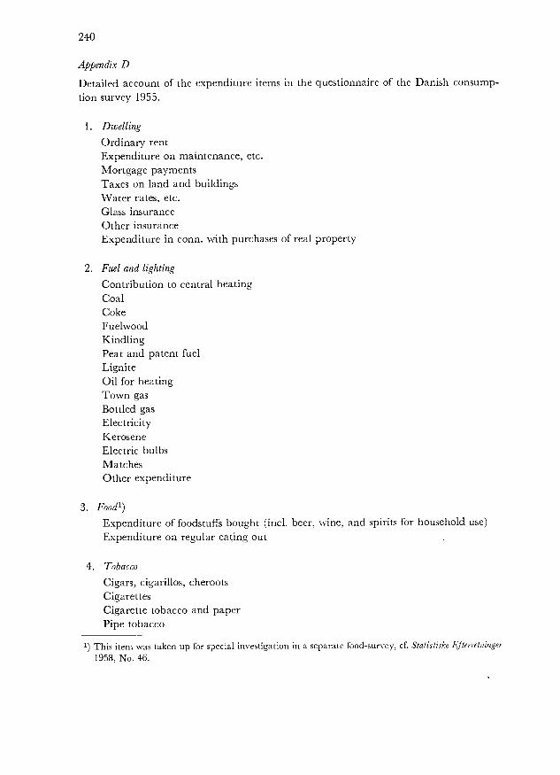
240

Appendix D

Detailed account of the expenditure items in the questionnaire of the Danish consumption survey 1955.

Dwelling

Ordinary rentExpenditure on maintenance, etc.Mortgage paymentsTaxes on land and buildingsWater rates, etc.Glass insuranceOther insuranceExpenditure in conn. with purchases of real property

Fuel and lighting

Contribution to central heatingCoalCokeFuelwoodKindlingPeat and patent fuelLigniteOil for heatingTown gasBottled gasElectricityKeroseneElectric bulbsMatchesOther expenditure

Food')

Expenditure of foodstuffs bought (incl, beer, vine, and spirits for household use)Expenditure on regular eating out

Tobacco

Cigars, cigarillos, cherootsCigarettesCigarette tobacco and paperPipe tobacco

1) This item was taken up for special investigation in a separate food-survey, cf. Statistiske Efterretninger1958, No. 46.

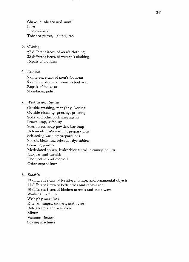
Chewing tobacco and snuffPipesPipe cleanersTobacco purses, lighters, etc.

Clothing

27 different items of men's clothing25 different items of women's clothingRepair of clothing

Footwear

5 different items of men's footwear5 different items of women's footwearRepair of footwearShoe-laces, polish

Washing and cleaning

Outside washing, mangling, ironingOutside cleaning, pressing, proofingSoda and other softening agentsBrown soap, soft soapSoap flakes, soap powder, bar-soapDetergents, dish-washing preparationsSelf-acting washing preparationsStarch, bleaching solution, dye tabletsScouring powderMethylated spirits, hydrochloric acid, cleaning liquidsLacquer and varnishFloor polish and mop-oilOther expenditure

Durables

13 different items of furniture, lamps, and ornamental objects11 different items of bedclothes and table-linen10 different items of kitchen utensils and table wareWashing machinesWringing machinesKitchen ranges, cookers, and ovensRefrigerators and ice-boxesMixersVacuum-cleanersSewing machines

241

242

PerambulatorsBrushesBuckets, tubsIronsTools and implements (excl, those for professional use, hobby, and garden)Other acquisitions apart from transport equipmentRepair of durables

Personal hygiene

Bath, pedicure, ultra-violet ray treatmentHairdresser and beauty cultureHand soap, bathing soap, shaving soapHair-washing preparationsToothpasteNail brushes, sponges, face chothsCombs, hairbrushes, hairpinsRazor, shaversToothbrushes and tooth glassesHair-lotion, brilliantine, cream, perfume, lipstick, powder, nail-polish, and other

cosmetic articlesOther expenditure on personal hygiene

Books, newspapers, etc.

BooksNewspapersWeekly and monthly magazinesPeriodicals

Sports, hobbies

Consumption at restaurantsBeer, wine, and spirits outside the usual household consumptionRadio and televisionGramophoneMusical instrumentsTheatre, cinema, and concertsOther entertainment (sports games, etc.)Holiday dwellingOther holiday expenditure, incl, holiday transportGarden and domestic animalsSports, subscriptions, and accessoriesOther recreation

Transport

Public transport facilitiesTaxiAcquisition and maintenance of bicycleAcquisition and maintenance of motor-assisted bicycleAcquisition and maintenance of motor-car and motor-cyclePetrol and ailTaxes and insuranceOther transport expenditure

Union fees and subscriptions

Unemployment insuranceFire and burglary insuranceHealth insuranceOther insurance (excl, life and superannuation insurance)Fees and subscriptions to trade and professional associationsOther fees and subscriptions (excl, sports and motor associations)

243