incorporating gene networks into statistical tests for genomic

Research Report , 1–25

Incorporating Gene Networks into Statistical Tests for Genomic Data via a

Spatially Correlated Mixture Model

Peng Wei∗ and Wei Pan∗∗

Division of Biostatistics, School of Public Health

University of Minnesota, A460 Mayo Building (MMC 303), Minneapolis, MN 55455-0378, USA

Phone number: (612)626-2705

Fax:(612)626-0660

*email: [email protected]

**email: [email protected]

Summary: It is a common task in genomic studies to identify a subset of the genes satisfying

certain conditions, such as differentially expressed genes or regulatory target genes of a transcription

factor (TF). This can be formulated as a statistical hypothesis testing problem. Most existing

approaches treat the genes as having an identical and independent distribution a priori, testing

each gene independently or testing some subsets of the genes one by one. On the other hand, it is

known that the genes work coordinately as dictated by gene networks. Treating genes equally and

independently ignores the important information contained in gene networks, leading to inefficient

analysis and reduced power. We propose incorporating gene network information into statistical

analysis of genomic data. Specifically, rather than treating the genes equally and independently a

priori in a standard mixture model, we assume that gene-specific prior probabilities are correlated

as induced by a gene network: while the genes are allowed to have different prior probabilities, those

neighboring ones in the network have similar prior probabilities, reflecting their shared biological

functions. We applied the two approaches to a real ChIP-chip dataset (and simulated data) to identify

the transcriptional target genes of TF GCN4. The new method was found to be more powerful in

discovering the target genes.

Key words: ChIP-chip; Conditional autoregression model; Markov random field; Transcription

factor.

1

Gene Networks in Analysis of Genomic Data 1

1. Introduction

High-throughput microarray technologies have been widely used in genomic studies. For

example, cDNA and Affymetrix arrays are used to monitor genome-wide gene expression,

while ChIP-chip, a hybrid of chromatin immunoprecipitation and microarray technologies,

has been used to quantify occupancy of genomic promoter regions by a transcription factor

(TF). A common task in analyzing microarray data is to identify a subset of the genes satis-

fying certain user-specified requirements, for example, the genes with differential expression

between two experimental conditions or between tumors and normal tissues, or the genes

that are regulatory targets of a TF. The problem can be formulated as statistical hypothesis

testing: a null hypothesis, such as equal expression (EE) or non-target of a TF, and an

alternative one, usually the opposite of the null hypothesis, are specified for each gene;

statistical hypothesis testing is conducted on each gene. Many statistical methods have been

proposed for such a purpose, including SAM (Tusher et al. 2001), Empirical Bayes (EB)

methods (Efron et al. 2001, Newton et al. 2001), and Normal mixture models (Pan et al.

2002, McLachlan et al. 2006). Most methods, including all the above cited, treat the genes

equally and independently a priori. In particular, they ignore biological knowledge about gene

functions and biological pathways. There have been increasing efforts recently to incorporate

biological knowledge into statistical analysis of microarray data to gain statistical efficiency.

For example, Pan (2005, 2006) proposed a stratified mixture model to incorporate gene

functions as annotated in the Gene Ontology (GO) database (Ashburner et al. 2000); Xiao

et al (2005) developed a Hidden Markov Model to incorporate genomic location information

into analysis, accounting for spatial patterns of gene co-expression. Another class of emerging

methods is to analyze gene sets, rather than individual genes; the gene sets are formed based

on biological pathways or gene functional groups (Subramanian et al 2005; Tian et al 2005;

Efron et al 2007; Newton et al 2007). Nevertheless, each of the gene-set methods treats the

2

genes equally and independently a priori, and the results depend on the specification of gene

sets: a too large or too small gene set may lead to reduced statistical power; in fact, each

gene set can be regarded as a gene subnetwork. As biological knowledge accumulates rapidly,

genome-wide gene networks represented by undirected graphs with genes as nodes and gene-

gene interactions as edges have been constructed; see Lee et al. (2004) for a probabilistic

approach to constructing functional networks for the yeast genome and Franke et al (2006)

for a human protein-protein interaction network. However, there has been very limited work

attempting to incorporate genome-wide gene network information into statistical analysis

of microarray data. An exception goes to the recent work by Wei and Li (2007) (see also

references therein), who proposed integrating KEGG pathways or other gene networks into

analysis of differential gene expression via a Markov Random Field (MRF) model.

Unlike directly modeling the state of each gene via a MRF (Wei and Li 2007), we propose

modeling some latent variables related to the prior probability of each gene’s being in a state

via MRFs, leading to a spatially correlated mixture model. The spatial mixture model was

first proposed by Fernandez and Green (2002) in spatial statistics, and applied to analyze

comparative genomic hybridization (CGH) data by Broet et al (2006). This is in contrast to

standard mixture models. For example, McLachlan et al. (2006) proposed using a standard

two-component normal mixture model to identify differentially expressed genes; although

promising results have been obtained, one key assumption of the standard normal mixture

model is that all genes share the same prior probability of coming from a component of the

normal mixture without regard to their biological functions. In the context of CGH data

analysis, Broet et al. (2006) proposed using a spatially correlated normal mixture model to

introduce gene-specific prior probabilities and allow those prior probabilities to be correlated

among neighboring genes on a chromosome, and gained more power to identify gene copy

number changes. Extending the work of Broet et al from one-dimensional chromosome


locations to two-dimensional gene networks, we propose using the spatially correlated normal

mixture model to improve power in identifying differentially expressed genes (for cDNA,

Affymetrix or any other expression arrays) or target genes of a TF (for ChIP-chip data). A

key difference from Broet et al is our utilizing existing biological knowledge databases, such

as KEGG pathways (Kanehisa and Goto 2000), or computationally predicted gene networks

from integrated analysis (Lee et al. 2004), to construct gene functional neighborhoods and

incorporating them into a spatially correlated normal mixture model. The basic rationale

underlying the proposed model is that functionally linked genes tend to be co-regulated and

co-expressed, which is thus incorporated into analysis.

The rest of this paper is organized as follows. We first review the standard normal mixture

model, then propose the spatially correlated normal mixture model. For illustration, we apply

and compare the two methods using a ChIP-chip dataset to identify the target genes of TF

GCN4. A simulated data set is also used to demonstrate the advantage of the proposed

method over the standard mixture model. Finally, we summarize our results and outline

some future work.

2. Methods

2.1 Problem

The goal of analysis is to identify which genes satisfy a certain condition, such as being

differentially expressed (DE) or being a TF’s transcriptional targets. It can be formulated as

a formal or informal hypothesis testing problem: for each gene i, we test for a null hypothesis

H0,i against an alternative hypothesis H1,i, usually the opposite of H0,i. For example, H0,i is

that “gene i is equally expressed (EE)” for expression data, or that “gene i is not a target

of the TF” for ChIP-chip data, while H1,i is the opposite of H0,i.

We assume that the data have been summarized as measurement Zi for each gene i, i =

4

1, . . . , G; for example, Zi can be a test statistic measuring the relative abundance of mRNA

(or TF), or the statistical significance level for rejecting H0,i. Define Ti = I(H0,i is false);

that is, Ti = 1 or Ti = 0 corresponds to that H1,i or H0,i holds respectively.

For our real data, we extracted a p-value for each gene, then transformed it to a z-score

and subsequently model the z-scores (McLachlan et al 2006). The transformation is given

by zi = Φ−1(1−Pi), where Φ is the cumulative distribution function of the standard Normal

distribution N(0, 1), and Pi is the p-value for gene i. If Pi is properly calculated as a genuine

p-value, then the null distribution of zi is exactly the standard normal. In addition, the

non-null distribution may model the right-tail of the z-score distribution. The resulting two-

component normal mixture model is

f(zi) = π0φ(zi; 0, 1) + π1φ(zi; µ1, σ21),

where φ(·; µ, σ2) is the probability density function of N(µ, σ2). However, sometimes the

null distribution of the z-scores is not standard normal due to approximate p-values (e.g.,

resulting from possible correlations among the genes, in contrary to the adopted indepen-

dence assumption). In this situation, we need to estimate the null distribution N(µ0, σ20).

We call N(0, 1) theoretical null and φ(µ̂0, σ̂02) empirical null. Furthermore, more than two

components may be needed for f .

2.2 Gene networks

The types of gene networks that can be used here are not restrictive; it can be any network as

long as the basic assumption holds: based on a gene network, two neighboring genes (i.e. two

genes with an edge between them) are more likely to satisfy H0,i or H1,i at the same time

than two non-neighboring genes. As stated before, a gene network can be extracted from

existing biological databases, such as KEGG pathways, or any computationally predicted

gene network, possibly resulting from integrated analysis of multiple sources of genomic data.

In this paper, we use the functional linkage network of yeast genes constructed by Lee et al


(2004) as an example. Lee et al applied a naive Bayes method to assign a score to each possible

gene pair by integrating a variety of genomic data, including mRNA co-expressions, gene

co-citations, protein-protein interactions, gene fusions and phylogenetic profiles. Two genes

with a score high enough are linked, suggesting that it is highly likely that they share some

biological function. They obtained a gene network called ’ConfidentNet’ with high credibility.

Represented by an undirected graph, the ’ConfidentNet’ consists of 4,681 nodes (genes) and

34,000 edges (gene-gene functional linkages). A summary of the distribution of the number

of direct neighbors is: minimum=1, 25th-percentile=2, median=6, 75th-percentile=13 and

maximum=188. We will use this yeast gene network in our real data example.

2.3 Standard Normal Mixture Model

Suppose that the distribution functions of the data (e.g. z-scores) for the genes with Ti = 1

and Ti = 0 are f1 and f0, respectively. Assuming that a priori all the genes have an identical

and independent distribution (iid), we have a marginal distribution of Zi as a standard

mixture model:

f(zi) = π0f0(zi) + (1 − π0)f1(zi), (1)

where π0 is the prior probability that H0,i holds. It is worth noting that the prior probabilities

are the same for all genes. The standard mixture model has been widely used in microarray

data analysis (e.g. Efron et al 2001; Newton et al 2001; Pan et al 2002; Broet et al 2006;

McLachlan et al 2006).

The null and non-null distributions f0 and f1 can be approximated by finite normal

mixtures: f0 =∑K0

k0=1 π0k0φ(µk0

, σ2k0

) and f1 =∑K1

k1=1 π1k1φ(µk1

, σ2k1

), where φ(µ, σ2) is the

density function for a Normal distribution with mean µ and variance σ2. For z-scores, using

Kj = 1 often suffices (McLachlan et al 2006). In our real data example, we found that K0 = 2

and K1 = 1 worked well.

The standard mixture model can be fitted via maximum likelihood with the EM algorithm

6

(McLachlan and Peel 2000). Once the parameter estimates are obtained, statistical inference

is based on the posterior probability that H1,i holds: Pr(Ti = 1|zi) = π1f1(zi)/f(zi). Because

the spatially correlated mixture model is fitted in a Bayesian framework while it is unclear

how to fit it in a frequentist approach, to facilitate comparison, we fitted the standard mixture

model in a similar Bayesian framework; see below for prior specifications.

2.4 Spatial Normal Mixture Model

In a spatial normal mixture model, we introduce gene-specific prior probabilities πi,j =

Pr(Ti = j) for i = 1, . . . , G and j = 0, 1. Hence, the marginal distribution of zi is

f(zi) = πi,0f0(zi) + πi,1f1(zi). (2)

Note that the prior probability specification in a stratified mixture model (Pan 2005, 2006,

2006b) is a special case of (2): a group of the genes with the same function share a common

prior probability while different groups have possibly varying prior probabilities; in fact, a

partition of the genes by their functions can be regarded as a special gene network.

Based on a gene network, we relate the prior probabilities πi,j to two latent Markov random

fields xj = {xi,j ; i = 1, ..., G} by a logistic transformation:

πi,j = exp(xi,j)/[exp(xi,0) + exp(xi,1)].

Each of the G-dimensional latent vectors xj is distributed according to an intrinsic Gaussian

conditional autoregression model (ICAR) (Besag and Kooperberg 1995). One key feature of

ICAR is the Markovian interpretation of the latent variables’ conditional distributions: the

distribution of each spatial latent variable xi,j, conditional on x(−i),j = {xk,j; k 6= i}, depends

only on its direct neighbors. More specifically, we have

xi,j |x(−i),j ∼ N

1

mi

∑

l∈δi

xl,j,σ2

Cj

mi

,

where δi is the set of indices for the neighbors of gene i, and mi is the corresponding number

of neighbors. To allow identifiability, we impose∑

i xij = 0 for j = 0, 1. In this model, the


parameter σ2Cj acts as a smoothing prior for the spatial field and consequently controls the

degree of dependency among the prior probabilities of the genes across the genome: the

smaller σ2Cj induces more similar πi,j ’s for those genes that are neighbors in the network.

In summary, it is biologically reasonable to assume that the neighboring genes in a network

are more likely to share biological functions and thus to participate in the same biological

processes. Hence they should have similar prior probabilities of being DE or being targets of

a TF at the same time.

2.5 Prior distributions

We largely followed Broet et al’s prior specifications. For either mixture model, we use

vague or noninformative prior distributions: µ0 = 0, µ1 ∼ N(0, 106)I(a, 0), a truncated

normal distribution between a = mini zi and 0; µ2 ∼ N(0, 106)I(0, b) and b = maxi zi. The

two truncated normals are constructed to ensure unique labeling of the normal mixture

components. In addition, we have σ2j ∼ Inverse Gamma(0.1, 0.1) for j = 0, 1, 2. See section

3.2.3 for discussions on selection of hyperparameters in the Inverse Gamma distrubution.

For the standard mixture model, (π0, π1, π2) ∼ Dirichlet(1, 1, 1). For the spatial mixture

model, σ2Cj ∼ Inverse Gamma(0.01, 0.01) for j = 0, 1, 2. Notice that the precision parameter,

τCj = 1/σ2Cj, has Gamma(0.01, 0.01) with mean 1 and variance 100.

For completeness, the details of the model specifications for both spatial and standard

normal mixture models are given in the Appendix.

2.6 Inference

Each of the above mixture models can be readily implemented in WinBUGS (Spiegelhalter

et al, 2003). The posterior mean of any parameter based on Markov Chain Monte Carlo

(MCMC) samples is used as its point estimate. In particular, based on whether the point

estimate P̂ r(H0,i|data) is smaller than a threshold c, we determine whether to reject H0.

There is a correspondence between c and false discovery rate (FDR), which can be estimated

8

based on P̂ r(H0,i|data). In this paper, we consider varying c, leading to various sensitivities

and specificities and thus yielding an ROC plot.

3. Results

3.1 Real data

3.1.1 Data. To evaluate the performance of our proposed method, we applied the two

methods - standard normal mixture model, denoted as Independence model, and spatial

normal mixture model, denoted as Spatial model - to a ChIP-chip data set for transcrip-

tion factor GCN4. A TF is a protein that binds to the promoter regions of its regulatory

target genes and participates in the recruitment of RNA polymerase, thus regulating the

transcription of its target genes into messenger RNA. ChIP-chip is a hybrid of chromatin-

immunoprecipitation (ChIP) and microarray technology that is used to quantify the occu-

pancy of genome-wide promoter regions by a TF. A typical ChIP-chip data set contains log

binding ratios measuring the relative abundances of the TF bound to the genes, and possibly

inferred statistical significance levels (p-values) for rejecting the null hypothesis that each

of the genes is not bound by the TF. As a TF, GCN4 is involved in response to amino

acid starvation in yeast. Lee et al. (2002) did ChIP-chip experiments for GCN4 with three

replicates. Log binding ratios and p-values for 6,181 yeast genes were provided. Pokholok

et al. (2005) constructed a set of 80 genes that are very likely to be the binding targets

of GCN4 from multiple sources of data (including another set of more accurate ChIP-chip

experiments based on a new generation of microarrays, a gene expression data set, and DNA

motif analyses), as well as a set of 900 genes that are unlikely to be regulated by GCN4.

Treating the positive and negative control sets as the true positives and true negatives, we

used them to evaluate the performance of the two methods; that is, sensitivity and specificity

were calculated based on the two control sets. In addition, for the spatial normal mixture


model, we used the yeast gene network constructed by Lee et al. (2004) to specify gene

neighborhoods. After merging the ChIP-chip data set and the gene network, we ended up

with a 4616-node network with 33,432 edges. We extracted those 4,616 genes’ binding p-

values and obtained their z-scores for final analysis; correspondingly, there were 66 and 770

genes in the positive and negative control sets respectively.

[Figure 1 about here.]

For illustration, a subnetwork consisting of only the positive and negative control genes

is shown in Figure 1, where dark nodes represent the target genes (positive controls) while

blank ones as non-targets (negative controls). Several features are noticeable. First, there is a

cluster of positive control genes in the upper-right corner, and there are quite a few clusters

of negative control genes. Second, positive control genes can be connected with negative

control genes. Third, although there are many singletons (i.e. isolated genes without edges

to other genes) in the subnetwork, they are not necessarily singletons in the whole network

because they may be connected to other genes outside the control sets. We used the full

network.

3.1.2 Model fitting. WinBUGS (Spiegelhalter et al. 2004) was used to implement the

Bayesian models. Posterior means of the parameters were computed based on 4,000 MCMC

samples after 6,000 burn-ins. First, a standard two-component normal mixture model with

an empirical null distribution (i.e. its mean and variance parameters were unknown and

needed to be estimated) was fitted; lack-of-fit of the mixture model against the data was

observed (results not shown). To achieve better model fit, a third normal component with

mean imposed to be negative was added into f0; the fitted mixture model was

f̂(zi) = 0.91φ(zi; 0, .802) + 0.037φ(zi;−1.98, .402) +

0.058φ(zi; 1.67, 1.942),

10

where the first two components with zero and negative means were treated as f̂0 and the

third one with postive mean as f̂1. A visual examination revealed improved goodness-of-fit

except at the peak of the data distribution (Figure 2). Similarly, a three-component spatial

normal mixture model with an empirical null was fitted, yielding

f̂(zi) = π̂i,0,1φ(zi; 0, .632) + π̂i,0,2φ(zi;−0.38, 1.022) +

π̂i,1,1φ(zi; 0.75, 1.532)

with the averages of π̂i,0,1, π̂i,0,2 and π̂i,1,1 as 0.500, 0.314 and 0.186. The fitted marginal and

component-wise distributions are displayed in Figure 2. We used different initial values to

look at the convergence of the MCMC simulations. Trace plots showed good convergence for

all the models (Figure 3).



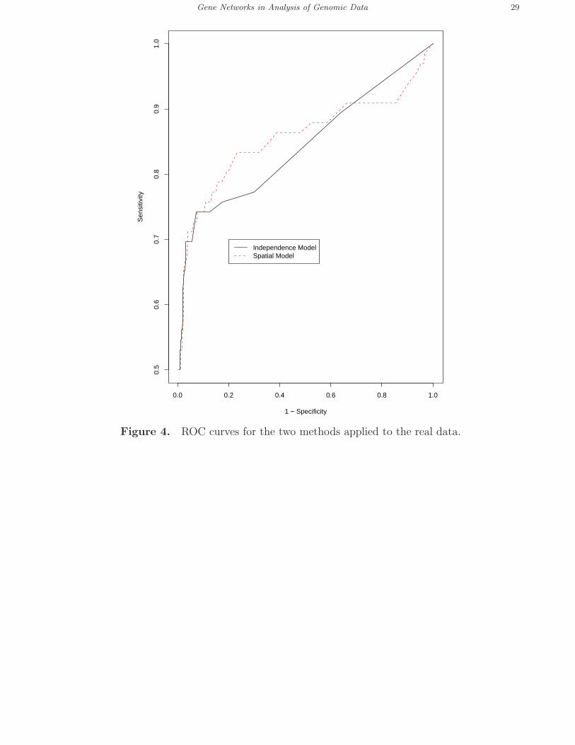
3.1.3 Statistical power. The ROC curves were constructed for the two methods based on

the positive and negative control sets. As shown in Figure 4, when the specificity ranged from

0.9 to 0.4, as desired in practice, the spatial normal mixture model gave a higher sensitivity

than that of the standard normal mixture model. Hence, at a high specificity (e.g. above 0.5

as usually desired), by taking use of biological knowledge embedded in a gene network, the

spatial normal mixture model had higher statistical power to detect the targets than did the

standard mixture model that ignored biological knowledge.

In addition, we compared the positive control genes’ ranks by the posterior probabilies from

the spatial model and the original binding p-values. As shown in Figure 5(b), most of the

positive control genes were ranked in the top 100 by both methods, while the spatial model

boosted a few more genes’ ranks from moderate (ranked between 200 - 400) to relatively high


(ranked between 100 - 200). There were about equally many positive control genes ranked

low by either method, as illustrated by the upper-right part of Figure 5(a).



3.1.4 Representative gene evaluations. We examined several individual genes to gain

more biological insights. First, for ARG8 (YOL140W), a gene in the positive control set,

its posterior probability of being a target was estimated to be 0.728 by the spatial model

and 0.023 by the independence model. The binding ratio for this gene in Lee et al.’s rich

medium ChIP-chip experiment was 1.02. However, Harbison et al.(2004) did more ChIP-chip

experiments on GCN4 in amino acid starvation and nutrition deprivation conditions besides

rich medium, and the binding ratio for ARG8 was 5.0 with p-value 10−11. Because GCN4

is a transcriptional activator of amino acid biosynthetic genes in response to amino acid

starvation, it is expected that genes involved in amino acid biosynthetic process are likely to

be binding targets of GCN4. In fact, ARG8 is known to be involved in arginine and ornithine

biosynthetic processes (Pauwel et al. 2003, Jauniaux et al. 1978), and is annotated in GO

Biological Process: amino acid biosynthetic process (GO ID:0008652). Note that ARG8,

located in the upper-right cluster of positive control genes in Figure 1, is a direct neighbor of

four other positive control genes but none of the negative control genes. We conjecture that

its positive neighbors explain why ARG8’s gene specific prior probability of being a target

was estimated to be 0.733 by the spatial model, in contrast to 0.058 by the independence

model; the high prior probability boosted its posterior probability of being a target. Second,

TRP5 (YGL026C) is a gene in neither control set, but it is a direct neighbor of ARG8. Its

gene specific prior probability of being a target was estimated to be 0.716 by the spatial

model, as compared to 0.058 by the independence model, and the posterior probability was

estimated to be 0.723 by the spatial model and to be 0.032 by the independence model. The

12

binding ratios for this gene were 1.15 and 1.21 in Lee et al’s and Harbison et al’s experiments

respectively. However, Beyer et al. (2006) computationally predicted TRP5 to be a binding

target of GCN4 with a high confidence level by integrating multiple data sources. In addition,

TRP5 is known to participate in trytophan biosynthetic process (Elion et al. 1991, Toyn et

al. 2000), and also annotated in GO Biological Process: amino acid biosynthetic process (GO

ID:0008652). Hence, it is a likely target of GCN4. Finally, we looked at a positive control

gene, ICY2 (YPL250C). It has six direct neighbors in the network: two of them are in the

negative control set and none of them are in the postive control set. Its prior and posterior

probabilities of being a target were estimated to be 0.668 and 0.836 respectively by the

spatial model; in contrast, the independence model gave estimates of the prior and posterior

probabilities to be 0.058 and 0.548 respectively. Two of its direct neighbors are negative

control genes, ADY2 (YCR010C) and CRS5 (YOR031W), whose prior probabilities of being

a target were estimated to be 0.08 and 0.12 respectively by the spatial model, as compared to

0.058 for both by the independence model; their posterior probabilities of being a target were

0.06, 0.09 respectively by the spatial model, and 0.02, 0.02 respectively by the independence

model. Therefore, although ICY2 is surrounded by non-target genes in the network, it was

still identified as a binding target by the spatial model, while its neighboring negative control

genes were not identified as false positives. In summary, by taking use of biological knowledge

embedded in a gene network, the spatial normal mixture model had higher statistical power

to detect the targets than did the standard mixture model while maintaining a reasonable

specificity.

3.2 Simulated data

3.2.1 Simulation set-up. To further investigate the property of our proposed method, we

conducted a simulation study that mimicked real data: we simulated a gene network similar

to the one used for the real data, and used data-generating distributions similar to the ones


fitted to the real data. We used Wei and Li’s discrete local MRF model to generate the true

binding (or differential expression) states for simulated data. Suppose for a network of G

genes, we have the binding state vector y = (y1, y2, . . . , yG), which is modeled by a MRF

with parameter Φ = (γ0, γ1, β). More specifically, we have

p(y; Φ) ∝ exp(γ0n0 + γ1n1 − βn01),

where n0 =∑G

i (1− yi) is the number of genes at state 0 with Hi,0 holding, n1 =∑G

i yi is the

number of genes at state 1 with Hi,1 holding, and n01 is the number of the network edges

linking two genes at two different states. It follows that the conditional probability of gene

i at state j given all the states of other genes is

pi(j|.) ∝ exp(γj − βui(1 − j)), (3)

where ui(1 − j) is the number of the neighbors of gene i that have state (1 − j), j = 0, 1.

To generate simulated data, for simplicity we first removed 7 singletons from the yeast gene

network and ended up with a 4609-node and 33,432-edge network. Second, to simulate y,

the latent binding states, we initialized the 66 genes in the positive control set to be binding

targets and the rest of genes to be non-targets, giving an initial y. Then we iterated the states

20 times based on Equation (3), with γ0 = 1, γ1 = 1, β = 2. It turned out that the number of

binding targets became stable at about 170 after ten iterations, and we chose the states to be

the ones right after the 10th iteration, giving 183 binding targets. Hence, the generated true

state vector y was only an approximation to a MRF, lending the opportunity to investigate

the robustness of the spatial mixture model. Note that our spatial mixture model assumes

an exact MRF for the latent variables x related to prior probabilities, not a MRF for the

latent binding states y, giving our model another source of model mis-specification. Next,

given y, we simulated the z-scores according to the fitted spatial mixture model from the

real data; for simplicity, we only used the null and positive components, i.e., φ(0, 0.632) and

φ(0.75, 1.532).

14


3.2.2 Simulation results. We simulated 5 data sets according to the above procedure, and

fitted the two-component spatial mixture model and standard mixture model as described

in the previous section. To compare their performance, we plotted the ROC curves for these

two methods as shown in Figure 4. Curves in the same color (or gray level) are for the

same simulated dataset. Note that for each pair, the spatial mixture model won for any

given specificity ranging from 10% to 95%. The average gain of sensitivity was about 10% at

specificity 80%, while the average gain could reach 20% at specificity 50%. It was confirmed

that again the spatial mixture model gave a much higher sensitivity at a given specificity as

compared to the standard independence mixture model.

3.2.3 Sensitivity analysis. Because of imcomplete biological knowledge, it is likely that

a gene network contains false positive edges while missing some true ones. To evaluate the

impact of misspecified network, we perturbed the network generated in the simulation. More

specifically, we perturbed the network in three ways. In scenario 1, we randomly removed

5% (1672) edges from the original 33,432-edge network, and it resulted in 46 singletons.

We eliminated those singletons by randomly connecting each of them to another gene and

ended up with a 31,806-edge network. In scenario 2, we randomly added 1672 edges to the

original network, and thus had a 33,432-edge new network. Third, we removed the same set

of 1672 edges as in scenario 1 from, then added the same set of 1672 edges as in scenario 2

to the original network; further more, we eliminated 20 singletons by randomly connecting

each of them of another gene, ending up with a 33,452-edge network. We applied the three

perturbed networks as well as the true network to one of the aforementioned simulated data

sets, and constructed the corresponding ROCs as shown in Figure 7. We see that removing

a small percentage of edges did not seem to affect the results much (first scenario), while

adding a small percentage of edges affected the results a bit more (second scenario). When


the network contains both false negative and false positive edges as in the third scenario,

the results seemed to be affected most substantially. Nevertheless, even in the third scenario

the spatial model performed no worse than the independence model. Consequently, based

on our simulation study we conclude that our proposed spatial model is reasonably robust

to misspecified networks.

We also investigated how different hyperparameters of the prior distributions might influ-

ence the analysis results. In our current hyperparameter set-up, we imposed a moderately

informative prior on the variance/precision parameters of the normal mixture components,

i.e., the precision parameters had Gamma(0.1, 0.1) prior distribution with mean 1 and

variance 10, while other parameters had almost flat priors. We tried an almost noninformative

prior distribution, Gamma(0.0001, 0.0001), on the precision parameters as an alternative.

This Gamma distribution has mean 1 and variance 1000. Congdon (2001) pointed out

that if p(τ) ∼ Gamma(0.0001, 0.0001), the prior of τ will be approximately p(τ) ∼ 1/τ ,

which is known as Jeffrey’s prior and is a form of ‘reference prior’ intended to reflect our

ignorance about the parameter. We fitted the spatial model with these two hyperparameter

set-ups, Gamma(0.1, 0.1) and Gamma(0.0001, 0.0001), to the same simulated dataset as used

in the previous paragraph. The ROC curves are shown in Figure 8. We see that the two

independence model curves are tied together all the way, while the two spatial model curves

are first coupled with each other and then separated a little. either of the two curves from the

spatial model is well above those from the independence model. In addition, the posterior

distributions of the key parameters were also compared between the two spatial models and

they were all very close (Tables 1 & 2).



[Table 1 about here.]

16

[Table 2 about here.]

4. Discussion

In this paper, in contrast to the standard mixture model that treats the genes equally

and independently a priori, we have proposed a spatially correlated mixture model that

allows incorporating gene network information into statistical modeling of complex inter-

relationships among the genes. As expected, by borrowing information from a gene network

to account for coordinated functioning of the genes, the new method has potential to improve

statistical power for new discoveries with high-throughput genomic data. An application to

a ChIP-chip data set and simulated data demonstrated the utility and advantage of the

proposed method.

The proposed approach is in line with current efforts in integrating biological knowledge

and multiple types of data (Dopazo 2006): the gene network being used can be extracted

directly from existing biological databases, e.g. KEGG pathways, or can be computationally

predicted by integrative analysis of multiple types of data, as the gene function network

constructed by Lee et al (2004) and used in our example. In addition, the proposed method

covers the prior probability specification in a stratified mixture model used to incorporate

gene functional annotations (Pan 2005, 2006, 2006b) as a special case; in the latter, a

corresponding gene network may be regarded as the follows: each functional group is a

subnetwork consisting of the genes fully connected to each other, while there is no connection

between any two functional groups, and the smoothing parameter σCj in the ICAR model

is small enough (e.g. σCj = 0) to induce a constant prior probability for the genes within

the same functional group. Of course, the special case may be too restrictive: for example,

first, the genes within the same functional group may play different roles, not necessarily

sharing the same prior probability; second, different gene functional groups may interact to

each other, possibly through some genes with multiple functions. On the other hand, our


idea differs from existing approaches to using gene networks (Wei and Li 2007, and references

therein). For example, although there is a conceptual similarity between ours and that of

Wei and Li (2007) in the use of MRF to account for correlations among the genes, we model

the prior probabilities of genes’ being in a certain state, in contrast to the underlying true

states as modeled by Wei and Li, via a MRF. As a consequence, by the general result of the

consistency of the posterior probability relative to a specified prior distribution, we expect

that our method is more robust to misspecified gene networks than that of Wei and Li,

which may be more efficient if the gene network is correctly specified; due to incomplete

biological knowledge and prediction errors, it seems unlikely that a gene network can be

specified completely correctly. In addition, we use a Normal distribution for each component

of the mixture model while Wei and Li adopted the Gamma-Gamma model, although other

parametric models in either can be adopted; we use the Gaussian MRF for the latent variables

related to prior probabilities, in contrast to the binary MRF for the latent gene binding or DE

states. They have implications on the resulting estimation procedures: ours is fully Bayesian

while Wei and Li used a pseudo-likelihood method, the iterative conditional mode (ICM)

algorithm (Besag 1986). Further studies to investigate the operating characteristics of our

proposal, including comparing its performance with others, and to extend our proposal to

more complex settings (e.g. Lewin et al 2006) will be interesting.

Acknowledgement

This research was partially supported by NIH grant HL65462 and a UM AHC Faculty

Research Development grant. The authors thank Stuart Levine and Rick Young for sharing

the binding data. The authors thank the reviewers for helpful and constructive comments.

18

5. Appedix

5.1 Model specifications

5.1.1 Model specification for a three-component standard normal mixture model. For i =

1, . . . , G; j = 0, 1, 2,

(Zi|Ti = j) ∼ N(µj , σ2j ),

P r(Ti = j) = πj ,

µ0 = 0; µ1 ∼ N(0, 106)I(a, 0), a = mini

zi,

µ2 ∼ N(0, 106)I(0, b), b = maxi

zi,

σ2j ∼ Inverse Gamma(0.1, 0.1), τj = 1/σ2

j ,

(π0, π1, π2) ∼ Dirichlet(1, 1, 1).

A two-component mixture model can be specified by dropping the negative component, as

used in the simulation.

5.1.2 Model specification for a three-component spatial normal mixture model. For i =

1, . . . , G; j = 0, 1, 2,

(Zi|Ti = j) ∼ N(µj , σ2j ),

P r(Ti = j) = πi,j = exp(xi,j)/[exp(xi,0) + exp(xi,1) + exp(xi,2)],

xi,j |x(−i),j ∼ N

1

mi

∑

l∈δi

xl,j ,σ2

Cj

mi

,

µ0 = 0; µ1 ∼ N(0, 106)I(a, 0), a = mini

zi,

µ2 ∼ N(0, 106)I(0, b), b = maxi

zi,

σ2j ∼ Inverse Gamma(0.1, 0.1), τj = 1/σ2

j ,

σ2Cj ∼ Inverse Gamma(0.01, 0.01), τCj = 1/σ2

Cj,


where∑

i xij = 0, for j = 0, 1, 2; δi is the set of indices for the neighbors of gene i, and mi =

|δi|. A two-component mixture model can be specified by dropping the negative component,

as used in the simulation.

5.2 WinBUGS codes for implementing the two methods

5.2.1 For a three-component standard normal mixture model.

model

{

for( i in 1:N ) {

Z[i] ~dnorm(muR[i], tauR[i]) # z-scores

muR[i] <- mu[T[i]]

tauR[i] <- tau[T[i]]

T[i] ~dcat(pi[ ]) # latent variable (zero/negative/postive components)

T1[i] <-equals(T[i],1) ;T2[i] <-equals(T[i],2); T3[i]<-equals(T[i],3);

}

# prior for mixing proportions

pi[1:3] ~ ddirch(alpha[])

# priors (means of normal mixture components)

mu[1] <- 0 # zero component

mu[2] ~dnorm(0, 1.0E-6)I(a, 0.0) #negative component

mu[3] ~dnorm(0, 1.0E-6)I(0.0, b) #positive component

# priors (precision/variance of normal mixture components)

tau[1]~dgamma(0.1, 0.1)

tau[2]~dgamma(0.1, 0.1)

tau[3]~dgamma(0.1, 0.1)

sigma2[1] <-1/tau[1]

20



}

5.2.2 For a three-component spatial normal mixture model.

model

{

for( i in 1:N ) {

Z[i] ~dnorm(muR[i], tauR[i]) # z-scores

muR[i] <- mu[T[i]]

tauR[i] <- tau[T[i]]

# logistic transformation

pi[i,1] <-1/(1+exp(x2[i]-x1[i])+exp(x3[i]-x1[i]))



T[i] ~dcat(pi[i,1:3]) # latent variable (zero/negative/postive components)

T1[i] <-equals(T[i],1) ;T2[i] <-equals(T[i],2); T3[i] <-equals(T[i],3)

}

# Random Fields specification

x1[1:N] ~car.normal(adj[], weights[], num[], tauC[1])



# weights specification

for(k in 1:sumNumNeigh) { weights[k] <- 1 }

# priors (precision/variance for MRF)


tauC[1] ~dgamma(0.01, 0.01)I(0.0001,)

tauC[2] ~dgamma(0.01, 0.01)I(0.0001,)

tauC[3] ~dgamma(0.01, 0.01)I(0.0001,)

sigma2C[1] <- 1/tauC[1]



# priors (means of normal mixture components)

mu[1] <- 0 # zero component

mu[2] ~dnorm(0, 1.0E-6)I(a,0.0) # negative component

mu[3] ~dnorm(0, 1.0E-6)I(0.0,b) # positive component

# priors (precision/variance of normal mixture components)

tau[1]~dgamma(0.1, 0.1)

tau[2]~dgamma(0.1, 0.1)

tau[3]~dgamma(0.1, 0.1)

sigma2[1] <- 1/tau[1]

sigma2[2] <- 1/tau[2]

sigma2[3] <- 1/tau[3]

}

References

Ashburner, M., et al. (2000) Gene ontology: tool for the unification of biology. The Gene

Ontology Consortium. Nature Genetics, 25, 25-29

Beyer, A., Workman, et al. (2006) Integrated assessment and prediction of transcription

factor binding. PLoS Computational Biology, 2:e70.

22

Besag, J. (1986) On the statistical analysis of dirty pictures. Journal of the Royal Statistical

Society: Series B, 48, 259-302.

Besag, J. and Kooperberg, C. (1995) On conditional and intrinsic autoregressions.

Biometrika, 82, 733-746.

Broet, P., Richardson, S. (2006) Detection of gene copy number changes in CGH microarrays

using a spatially correlated mixture model. Bioinformatics, 22, 911-918.

Congdon, P. (2001) Bayesian Statistical Modelling. Wiley, Chichester

Dopazo, J. (2006) Functional Interpretation of Microarray Experiments. OMICS: A Journal

of Integrative Biology, 10, 398-410.

Efron, B., et al. (2001) Empirical Bayes analysis of a microarray experiment. Journal of the

American Statistical Association, 96, 1151-1160.

Efron, B. and Tibshirani, R. (2007) On testing the significance of sets of genes. Annals of

Applied Statistics, 1, 107-129.

Elion, E.A., Brill, J.A., Fink, G.R. (1991) FUS3 represses CLN1 and CLN2 and in concert

with KSS1 promotes signal transduction. Proceedings of National Academy of Science,

88, 9392-6.

Fernandez, C. and Green, P. (2002) Modelling spatially correlated data via mixtures: a

Bayesian approach. Journal of the Royal Statistical Society: Series B, 64, 805-826.

Franke, L., van Bakel, H. (2006) Reconstruction of a Functional Human Gene Network, with

an Application for Prioritizing Positional Candidate Genes. The American Journal of

Human Genetics, 78, 1011-1025.

Harbison, C.T., Gordon, D.B. et al. (2004) Transcriptional Regulatory Code of a Eukaryotic

Genome. Nature, 431, 99-104

Jauniaux, J.C., Urrestarazu, L.A., Wiame, J.M. (1978) Arginine metabolism in Saccha-

romyces cerevisiae: subcellular localization of the enzymes. Journal of Bacteriology, 133,


1096-1107.

Kanehisa, M and Goto, S. (2000) Kegg: Kyoto encyclopedia of genes and genomes. Nucleic

Acids Res, 28, 27-30.

Lee, I., Date, S.V., Adai, A.T., Marcotte, E.M. (2004) Probabilistic Functional Network of

Yeast Genes. Science, 306, 1555 - 1558.

Lee, T.I., Rinaldi, N.J., Robert, F., Odom, D.T., Bar-Joseph, Z., Gerber, G.K., Hannett,

N.M., Harbison, C.T., Thompson, C.M., Simon, I. et al. (2002) Transcriptional regulatory

networks in Saccharomyces cerevisiae. Science, 298, 799-804.

Lewin A, Richardson S, Marshall C, Glazier A, Aitman T. (2006) Bayesian modeling of

differential gene expression. Biometrics, 62, 1-9.

McLachlan, G.J., Bean, R.W., Ben-Tovim Jones, L. (2006) A simple implementation of

a normal mixture approach to differential gene expression in multiclass microarrays.

Bioinformatics, 22, 1608-1615.

McLachlan, G.J., Peel, D. (2000) Finite Mixture Models. Wiley, New York

Newton, M.A., et al. (2001) On differential variability of expression ratios: improving

statistical inference about gene expression changes from microarray data. Journal of

Computational Biology, 8, 37-52.

Newton, M.A., Quintana, F.A., den Boon, J.A., Sengupta, S. and Ahlquist, P. (2007)

Random-set methods identify distinct aspects of the enrichment signal in gene-set

analysis. Annals of Applied Statistics, 1, 85-106.

Pan, W., Lin, J., Le, C. (2002) Model-Based Cluster Analysis of Microarray Gene Expression

Data. Genome Biology, 3, research0009.1-8.

Pan, W. (2005) Incorporating Biological Information as a Prior in an Empirical Bayes Ap-

proach to Analyzing Microarray Data. Statistical Applications in Genetics and Molecular

Biology, 4, Article 12.

24

Pan, W. (2006) Incorporating gene functional annotations in detecting differential gene

expression. Applied Statistics, 55, 301-316.

Pan, W. (2006b) Incorporating gene functions as priors in model-based clustering of microar-

ray gene expression data. Bioinformatics, 22, 795-801.

Pauwels, K., Abadjieva, A., Hilven, P., Stankiewicz, A., Crabeel, M. (2003) The N-

acetylglutamate synthase/N-acetylglutamate kinase metabolon of Saccharomyces cere-

visiae allows co-ordinated feedback regulation of the first two steps in arginine biosyn-

thesis. European Journal of Biochemistry, 270, 1014-24.

Pokholok, D.K., Harbison, C.T. et al. (2005) Genome-wide Map of Nucleosome Acetylation

and Methylation in Yeast. Cell. 122, 517-27.

Spiegelhalter, D., Thomas, A., Best, N., Lunn, D. (2003) WinBUGS User Manual, Version

1.4. Available at http://www.mrc-bsu.cam.ac.uk/bugs/winbugs/manual14.pdf

Subramanian, A. et al. (2005) Gene set enrichment analysis: a knowledge-based approach

for interpreting genome-wide expression profiles. Proceedings of National Academy of

Science, 102, 15545-15550.

Tian L, Greenberg SA, Kong SW, Altschuler J, Kohane IS, Park PJ. (2005) Discovering

statistically significant pathways in expression profiling studies. Proceedings of National

Academy of Science, 102, 13544-13549.

Toyn,J.H., Gunyuzlu, P.L., White, W.H., Thompson, L.A., Hollis, G.F.(2000) A counters-

election for the tryptophan pathway in yeast: 5-fluoroanthranilic acid resistance. Yeast,

16, 553-60.

Tusher, V.G., et al. (2001) Significance analysis of microarrays applied to the ionizing

radiation response. Proceedings of National Academy of Science, 98, 5116-5121.

Wei, Z., Li, H. (2007) A Markov Random Field Model for Network-based Analysis of Genomic

Data. Bioinformatics, 23, 1537-1544.


Xiao, G., Reilly, C., Martinez-Vaz, B., Pan, W., Khodursky, A.B. (2005) Improved de-

tection of differentially expressed genes through incorporation of gene locations. Re-

search Report 2005-028, Division of Biostatistics, University of Minnesota. Available at

http://www.biostat.umn.edu/rrs.php

November, 2007

26

p1

p2

p3

p4

p5

p6

p7

p8

p9

p10

p11

p12

p13

p14

p15

p16

p17

p18

p19

p20

p21

p22

p23

p24

p25

p26

p27

p28

p29

p30p31p32

p33

p34

p35

p36 p37

p38

p39

p40

p41

p42

p43

p44

p45

p46

p47

p48

p49

p50

p51

p52

p53

p54

p55

p56

p57

p58

p59

p60

p61

p62

p63

p64

p65

p66

n1

n2

n3

n4

n5

n6

n7n8

n9

n10

n11

n12

n13

n14

n15n16

n17

n18

n19

n20

n21

n22

n23

n24

n25

n26

n27

n28

n29

n30

n31

n32

n33n34

n35

n36

n37

n38

n39

n40

n41

n42

n43

n44

n45

n46

n47

n48

n49

n50

n51

n52n53

n54

n55

n56

n57

n58

n59

n60

n61

n62

n63

n64

n65

n66

n67

n68

n69

n70

n71

n72

n73

n74

n75

n76

n77

n78

n79

n80

n81

n82

n83

n84

n85

n86

n87n88

n89

n90

n91

n92

n93

n94

n95

n96

n97

n98

n99

n100

n101

n102

n103

n104

n105

n106

n107

n108

n109

n110

n111

n112

n113

n114

n115

n116

n117

n118

n119

n120

n121

n122

n123

n124n125

n126

n127

n128

n129

n130

n131

n132

n133

n134

n135

n136

n137

n138

n139

n140

n141

n142 n143

n144

n145

n146

n147

n148

n149

n150

n151

n152

n153

n154

n155

n156

n157

n158

n159

n160

n161

n162

n163

n164

n165

n166

n167

n168

n169

n170

n171

n172

n173

n174

n175

n176

n177

n178

n179

n180

n181

n182

n183

n184

n185

n186

n187

n188

n189

n190

n191

n192

n193n194

n195

n196

n197

n198

n199

n200

n201

n202

n203

n204

n205

n206

n207

n208

n209

n210

n211

n212

n213n214

n215

n216

n217

n218

n219

n220

n221

n222

n223n224

n225

n226

n227

n228

n229

n230

n231

n232

n233

n234

n235

n236

n237

n238

n239

n240

n241

n242

n243

n244

n245

n246

n247

n248

n249

n250n251

n252

n253

n254

n255

n256

n257

n258

n259

n260

n261

n262

n263

n264

n265

n266

n267

n268

n269

n270

n271

n272

n273

n274

n275

n276

n277

n278

n279

n280

n281

n282

n283

n284

n285

n286

n287

n288

n289

n290

n291

n292

n293

n294

n295

n296

n297

n298

n299

n300

n301

n302

n303

n304n305

n306

n307

n308

n309

n310n311n312

n313

n314

n315n316

n317

n318n319

n320

n321n322

n323n324

n325

n326

n327

n328

n329

n330

n331

n332

n333

n334

n335

n336

n337

n338

n339

n340n341

n342

n343

n344

n345

n346

n347 n348

n349

n350

n351n352

n353

n354

n355

n356

n357

n358

n359

n360

n361

n362

n363

n364

n365

n366

n367

n368

n369

n370

n371

n372

n373

n374

n375

n376 n377

n378

n379

n380

n381

n382

n383

n384

n385

n386

n387

n388

n389

n390n391n392

n393

n394

n395

n396

n397

n398n399

n400

n401

n402

n403

n404

n405

n406

n407

n408

n409

n410

n411

n412

n413n414

n415n416

n417

n418

n419

n420

n421

n422

n423

n424

n425

n426

n427

n428

n429

n430

n431

n432

n433

n434

n435

n436

n437

n438

n439n440

n441

n442

n443

n444

n445

n446

n447

n448

n449

n450

n451

n452

n453

n454

n455

n456

n457

n458

n459

n460

n461 n462

n463

n464

n465

n466

n467

n468

n469

n470

n471

n472

n473

n474

n475

n476

n477

n478

n479

n480

n481

n482

n483

n484

n485

n486

n487

n488

n489

n490

n491

n492

n493

n494

n495

n496

n497

n498

n499

n500

n501

n502

n503

n504

n505

n506

n507

n508

n509

n510

n511

n512

n513

n514

n515

n516

n517

n518

n519

n520

n521

n522

n523

n524

n525 n526

n527

n528

n529

n530

n531

n532 n533 n534

n535

n536

n537

n538n539n540

n541

n542

n543

n544

n545

n546n547n548n549n550n551

n552

n553

n554

n555

n556

n557

n558

n559

n560

n561

n562

n563

n564

n565

n566

n567

n568

n569

n570

n571

n572

n573

n574

n575

n576

n577

n578

n579

n580

n581

n582

n583

n584

n585

n586

n587

n588

n589

n590

n591

n592

n593

n594

n595

n596

n597

n598

n599

n600

n601n602n603

n604

n605

n606n607

n608

n609

n610

n611

n612

n613

n614

n615

n616

n617

n618 n619 n620

n621

n622

n623

n624

n625

n626

n627

n628

n629

n630

n631

n632

n633

n634

n635

n636

n637

n638

n639

n640

n641

n642

n643

n644

n645

n646

n647

n648

n649

n650 n651

n652

n653

n654

n655

n656

n657

n658

n659

n660

n661

n662

n663

n664

n665

n666

n667

n668

n669

n670n671

n672

n673

n674n675

n676

n677

n678

n679

n680n681n682n683

n684

n685

n686n687

n688

n689n690

n691

n692

n693

n694

n695

n696

n697

n698

n699

n700n701n702

n703

n704

n705

n706

n707

n708

n709

n710

n711

n712

n713

n714

n715

n716

n717

n718

n719

n720

n721

n722

n723

n724

n725

n726

n727

n728

n729

n730

n731

n732

n733

n734

n735

n736

n737

n738

n739

n740

n741

n742

n743

n744

n745 n746

n747

n748

n749 n750

n751

n752

n753

n754

n755

n756

n757

n758

n759

n760

n761

n762

n763

n764

n765

n766

n767

n768

n769

n770

Figure 1. Subnetwork consisting of positive control genes (dark ones) and negative controlgenes (black ones).


Independence Model

z−score

Den

sity

−4 −2 0 2 4 6

0.0

0.1

0.2

0.3

0.4

0.5

Spatial Model

z−score

Den

sity

−4 −2 0 2 4 6

0.0

0.1

0.2

0.3

0.4

0.5

Figure 2. Fitted mixture models: on each panel, the dashed line is for themarginal/mixture distribution while the three solid lines are for the three components.

28

0 5000 10000 15000

1.0

2.0

3.0

4.0

Spatial: τ0 = 1 σ02

Iterations

0 5000 10000 15000

0.0

0.5

1.0

1.5

2.0

2.5


Iterations

0 5000 10000 15000

0.2

0.4

0.6

0.8

1.0


Iterations

0 5000 10000 15000

−3

−2

−1

0

Spatial: µ1

Iterations

0 5000 10000 150000.

01.

02.

03.

0

Spatial: µ2

Iterations

0 5000 10000 15000

1.0

1.2

1.4

1.6

1.8

Independence: τ0 = 1 σ02

Iterations

0 5000 10000 15000

010

2030

4050

60


Iterations

0 5000 10000 15000

0.2

0.4

0.6

0.8


Iterations

0 5000 10000 15000−

4−

3−

2−

1

Independence: µ1

Iterations

0 5000 10000 15000

1.0

2.0

3.0

4.0

Independence: µ2

Iterations

0 5000 10000 15000

0.85

0.90

0.95

Independence: π0

Iterations

0 5000 10000 15000

0.00

0.02

0.04

0.06

Independence: π1

Iterations

Figure 3. Convergence check.


0.0 0.2 0.4 0.6 0.8 1.0

0.5

0.6

0.7

0.8

0.9

1.0

1 − Specificity

Sen

sitiv

ity

Independence ModelSpatial Model

Figure 4. ROC curves for the two methods applied to the real data.

30

0 200 400 600 800 1000

020

040

060

080

010

00

(a)

ranks by posterior probabilities from spatial model

rank

s by

orig

inal

bin

ding

p−

valu

es

0 100 200 300 400 500

010

020

030

040

050

0

(b)

ranks by posterior probabilities from spatial model

rank

s by

orig

inal

bin

ding

p−

valu

es

Figure 5. Comparison of positive control gene ranks by the posterior probabilities fromspatial model and the original binding p-values. Dotted diagonal is the identity line. (a) allthe positive control genes; (b) zoomed-in version of panel (a).


0.0 0.2 0.4 0.6 0.8 1.0

0.0

0.2

0.4

0.6

0.8

1.0

1−Specificity

Sen

sitiv

ity

Independence ModelSpatial Model

Figure 6. ROC curves for the two methods applied to five simulated data sets. Dashedlines are for the spatial model; solid lines are for the independence model.

32

0.0 0.2 0.4 0.6 0.8 1.0

0.0

0.2

0.4

0.6

0.8

1.0

1−Specificity

Sen

sitiv

ity

Spatial (true)Spatial (remove 5% edges)Spatial (add 5% edges)Spatial (remove and add 5%)Independence

Figure 7. ROC curves for misspecified network structures.


0.0 0.2 0.4 0.6 0.8 1.0

0.0

0.2

0.4

0.6

0.8

1.0

1−Specificity

Sen

sitiv

ity

Spatial, G(.1,.1)Spatial, G(.0001,.0001)Independence, G(.1,.1)Independence, G(.0001,.0001)

Figure 8. ROC curves for sensitivity analysis (two different priors for the precisionparameters of the normal mixture components).

34

Table 1

Posterior distributions of key parameters in the spatial model when using two different Gamma priors for theprecision parameters.

Parameter Prior Mean SD 2.5% Median 97.5%

µ2 G(.1,.1) 0.14 0.05 0.05 0.13 0.26

G(.0001,.0001) 0.11 0.04 0.04 0.11 0.18

τ1 G(.1,.1) 3.03 0.16 2.75 3.02 3.33

G(.0001,.0001) 3.08 0.11 2.88 3.08 3.30

τ2 G(.1,.1) 1.03 0.12 0.80 1.04 1.22

G(.0001,.0001) 1.06 0.06 0.94 1.06 1.18

τC1 G(.1,.1) 0.52 0.28 0.18 0.42 1.11

G(.0001,.0001) 0.80 0.34 0.31 0.72 1.49

τC2 G(.1,.1) 1.16 0.62 0.53 0.95 3.06

G(.0001,.0001) 1.22 0.49 0.38 1.21 2.24


Table 2

Posterior distributions of key parameters in the independence model when using two different Gamma priors for theprecision parameters.

Parameter Prior Mean SD 2.5% Median 97.5%

µ2 G(.1,.1) 0.53 0.21 0.20 0.49 1.05

G(.0001,.0001) 0.53 0.23 0.19 0.50 1.08

τ1 G(.1,.1) 2.50 0.09 2.33 2.49 2.67

G(.0001,.0001) 2.49 0.09 2.33 2.49 2.68

τ2 G(.1,.1) 0.55 0.10 0.36 0.55 0.75

G(.0001,.0001) 0.55 0.10 0.36 0.54 0.77

π1 G(.1,.1) 0.95 0.02 0.92 0.96 0.98

G(.0001,.0001) 0.95 0.02 0.91 0.96 0.98

π2 G(.1,.1) 0.05 0.02 0.02 0.04 0.08

G(.0001,.0001) 0.05 0.02 0.02 0.04 0.09

incorporating gene networks into statistical tests for genomic

Documents