ECINEQ WP 2017 - 438

Working Paper Series

Incorporating spatial price adjustments in

U.S. public policy analysis

John A. Bishop

Jonathan M. Lee

Lester A. Zeager

ECINEQ 2017 - 438May 2017

www.ecineq.org

Incorporating spatial price adjustments

in U.S. public policy analysis

John A. Bishop†

Jonathan M. Lee

Lester A. Zeager

East Carolina University, U.S.A.

Abstract

The U.S. Bureau of Economic Analysis has recently released regional price parities (RPPs)for the 325 Standard Metropolitan Statistical Areas and the 50 state nonmetropolitan areas.We consider the effects of RPP adjustments on four public policy issues: poverty rates, familyincome inequality, tax progressivity, and metropolitan-size premiums. We demonstrate thatRPP adjustments strongly affect the spatial distribution of U.S. poverty, have an equalizingeffect on income inequality (equivalent to a $1,500 cash transfer to each U.S. family), and alsoincrease effective federal tax progressivity by more than 25 percent. Income premiums for themajor metropolitan areas largely disappear after adjusting for spatial prices and controllingfor the characteristics of family heads. Metro-size premiums also depend on whether we ad-just incomes by the overall RPPs or a narrower housing-price index (as in earlier research).We conjecture that other public policy findings are sensitive to adjustments for spatial pricedifferences.

Keywords: regional price parities, poverty, inequality, tax progressivity, metro-size premiums.

JEL Classification: D31, H23, I32, R32.

†Contact details: all authors are at the Department of Economics East Carolina University, Greenville,NC 27858, USA. Emails: bishopj@ecu.edu (J.A. Bishop, corresponding author); leejo@ecu.edu (J.M. Lee) andzeagerl@ecu.edu (L.A. Zeager).

2

“National and international statistical systems are strangely reticent on differences in price

levels within countries. Nations as diverse as India and the United States publish inflation rates

for different areas, but provide nothing that allows comparison across places at a point in time.

The International Comparison Project, which at each round collects prices and calculates price

indexes for most of the countries of the world, publishes nothing on within country differences,

and in some important cases including China, Brazil, and India, rural prices are either not

collected or are underrepresented…" (Deaton and Dupriez 2011, 1)

Introduction

Nobel Prize winner Angus Deaton and the prestigious National Academy Panel on

Poverty and Family Assistance (Citro and Michael 1995) have called for the incorporation of

spatial price adjustments in public policy analysis. Albouy (2009, 636) also points out that the

U.S. federal tax code does not take into account variation in the cost of living across cities and

that, “Unlike local tax differences, federal tax differences of this kind are not compensated with

higher levels of local spending and may therefore affect location choices.” Deaton and Dupriez

(2011, 4) surmise that “the lack of these [spatial price] indexes more likely reflects the difficulty

and cost of producing them” rather than a lack of usefulness for policy purposes. In the United

States, these obstacles were recently overcome when the Bureau of Economic Analysis (BEA)

and the U.S. Census Bureau, working with the Bureau of Labor Statistics (BLS), released the

first official regional price parities (RPPs) for all U.S. metropolitan areas and state-level,

nonmetropolitan areas.1

We investigate the effects of spatial price adjustments on four public policy issues:

poverty rates, the degree of income inequality and tax progressivity, and metro-size premiums.

ECINEQ WP 2017 - 438 May 2017

3

As Deaton and Dupriez (2011, 1) observe, “… for the same reasons that we expect price levels to

be lower in poor countries—the Balassa-Samuelson theorem—we would expect prices to be

lower in poorer areas within countries, at least if people are not completely mobile across space.”

Comparing living standards across regions in the U.S. has much in common with comparing

poverty and inequality across countries in the world, but is less complicated, because in the

global comparisons the wider variation in consumption patterns makes it harder to estimate

relative prices. Deaton (2016, 1226) captures the dilemma,

On the one hand, we need to compare like with like, using only goods and

services that are close to identical in different countries. On the other hand, we

also wish to capture what people actually spend, so that we want to use goods and

services that are widely consumed and representative of actual purchases. These

two requirements often stand in sharp opposition; in the extreme case where

consumption bundles have nothing in common, there is no basis for comparisons

of living standards.

Deaton (2010) argues that comparisons are more meaningful for broadly similar countries and,

we add, still more so for regions within the same country.

For each of our policy issues (poverty, inequality, tax progressivity, and metro-size

premiums), we find significant changes after adjusting for spatial price differences. The RPP

adjustment has little effect on mean family money income, but has substantial effects on regional

poverty rates and virtually eliminates the difference in metro and nonmetro poverty rates.2 When

we take into account the tendency for high-income families to live in high-price areas, inequality

falls and effective federal tax progressivity increases by twenty-five percent. After adjusting for

ECINEQ WP 2017 - 438 May 2017

4

RPPs and controlling for family head characteristics, the higher family incomes found in major

metropolitan areas largely, but not completely, disappear.

Section 2 reviews the BEA procedures for generating the new RPP measures and

describes the resulting regional price differences. Section 3 shows how RPP adjustments affect

poverty, income inequality, and tax progressivity for U.S. primary families. Section 4 examines

the effect of RPP adjustments on urban size premiums. Section 5 reports the main findings and

suggests opportunities for future research.

Background and Data

As background for our analysis, we review some important steps leading to the

appearance of the official RPP indices. Three Budgets for an Urban Family of Four Persons

(Bureau of Labor Statistics 1979) was an early attempt by the BLS to measure regional living

costs. This measure was estimated for 25 metropolitan areas and for the nonmetro areas of the

four Census regions. Bishop, Formby, and Thistle (1992, 1994) used this series to study regional

income convergence in the U.S. and to create regional living cost indices for 1969 and 1979.

Unfortunately, the series was discontinued in the early 1980s.

Another important study, Measuring Poverty: A New Approach (Citro and Michael,

1995) by the National Academy Panel on Poverty and Family Assistance, raised the issue of

differences in prices across regions. It proposed using housing price indices to approximate the

regional price levels. As Deaton and Dupriez (2011, 4) have observed, “This proposal generated

a substantial subsequent research effort within federal statistical agencies,” particularly in regard

to the creation of a Supplemental Poverty Measure.3 Among all this research, the most important

ECINEQ WP 2017 - 438 May 2017

5

piece for our purposes is Aten, Figueroa, and Martin (2011), which is the primary source for

understanding the RPPs used in our analysis.

The New Regional Price Parities

This section provides an overview of the construction of the new RPP indices.4 We then

summarize the RPP data across metropolitan and nonmetropolitan areas, Census regions, and

divisions using the combined BEA and CPS datasets.

Beginning in 2003-2004, the BEA estimated U.S. regional price parities for the 38

metropolitan and urban areas that the BLS uses to generate the CPI, which contained about 87

percent of the U.S. population at that time.5 The procedure was based upon price information in

the CPI (covering hundreds of consumer goods and services) and used hedonic methods to adjust

for differences in product characteristics (type of outlet selling a good or service, packaging, etc.)

for the 75 most important item categories, representing about 85 percent of all expenditures. For

the remaining categories, a method roughly equivalent to a weighted geometric mean of prices in

each item category generated relative price levels. The estimation results were then checked for

outliers using methods similar to those developed for comparing relative prices across countries

in the Income Comparison Project.

The BEA extended the analysis beyond areas covered by the CPI in 2005-06, using

housing data from the American Community Survey (ACS). Housing is the key factor in the

cost of living; rents and owners’ equivalent rents are the most important consumer expenditure

category by far, accounting for 30 percent of the total. Once again, hedonic regression methods

allow adjustments for differences in housing characteristics (the number of rooms and bedrooms;

the age and type of housing unit). For all remaining goods and services, price levels for non-CPI

ECINEQ WP 2017 - 438 May 2017

6

areas are equated to the average for that region (e.g., the Midwest). The BEA released its official

real, per capita incomes for states and metropolitan statistical areas in April 2014, adjusted with

RPPs, i.e., percent differences in regional average prices from the national average (Aten and

Figueroa, 2014).

U.S. Price Level Differences

By construction, the national average price level is 100, and the RPPs for comparison

areas are expressed as percentages of the national average. Thus, the ratio RPP/100 gives the

relative price level for a comparison area. In 2012, the state metro areas with the highest RPPs

were Hawaii (122.7), the District of Columbia (118.7), New York (117.5), New Jersey (114.4),

and California (113.6). Arkansas (89), Alabama (89), Missouri (89.5), and West Virginia (90.1)

had the lowest metro RPPs among the states. The weighted-average price level in New Jersey is

about 14 percent higher (114.4/100) than the national average, and the price level in the District

of Columbia is about 33 percent higher than in Arkansas or Alabama (118.7/89 = 1.334). Aten,

Figeuroa, and Martin (2011) note that price levels across regions vary more for services (which

account for two-thirds of total consumer expenditures) than for goods. They report that, among

expenditure categories, housing rents vary the most and transportation costs (e.g., new and used

vehicle purchases) vary the least. Finally, they find that lower overall price levels in rural areas

are due primarily to lower housing and fuel prices.

Table 1 presents average RPP indices by metro status (plus the five SMSAs with the

highest and lowest overall price levels), region, race, age, and family money income, estimated

with 2012 BEA metro-level and state-level, nonmetro RPP indices and the 2013 CPS data (2012

incomes).6 The mean RPP for primary families is slightly less than 100 (99.7). The RPP index

ECINEQ WP 2017 - 438 May 2017

7

varies by metro status (nonmetro areas are the least expensive locations with an RPP of 87.9 on

average) and size (from 95.0, on average, for small metro areas to 109.3 for large metro areas).

The Northeast is the highest RPP region (108.8), followed by the West (106.0). The Midwest

(93.3) – not the traditionally poor South (95.5) – has the lowest population- weighted average

price level among regions. The comparisons by race show that Asians live in more expensive

areas (109.0) than whites (98.2), an 11 percent difference. Hispanics (103.7) also live is areas

slightly more expensive than whites. RPPs vary little by the age of the family heads, but they

increase with income, from 98.5 for families with incomes below $25,000 to 104.1 for families

with incomes above $150,000. Families identified by the U.S. Census Bureau as “poor” face

price levels (98.8) slightly below the U.S. average.

[place Table 1 about here]

U.S. Poverty and Inequality with RPP Adjustments

We begin by comparing the mean incomes, poverty rates, and Gini coefficients

constructed from the CPS microdata to those published by the U.S. Census. The attempt to

match the published figures gives us insight into the degree to which top-coding of incomes in

the public-use CPS files influences our findings. We make the comparisons with family money

income, the standard used in the published U.S. Census figures, which we construct from March

2013 CPS data. These figures provide a benchmark for assessing the effects of RPP adjustments.

Census family money income includes wages and salaries, self-employment income, dividends,

rent, interest, cash transfers (Social Security and Unemployment Insurance), and other cash

income, but it excludes the market value of in-kind transfers, the earned income tax credit, and

ECINEQ WP 2017 - 438 May 2017

8

all taxes. In spite of its shortcomings, Census money income is the basis for the most frequently

cited U.S. poverty and inequality statistics.7

Table 2 reports the mean family money income, the percentage of families below the

poverty level (with standard errors using Bishop, Formby and Zheng 1997), and the Ginis for

family money income (with standard errors using Bishop, Formby and Zheng 1998) in the U.S

overall, in metro areas, and in nonmetro areas. The figures in column (1), labeled “Census,” are

taken from the P-60 Series, “Income and Poverty in the United States, 2013,” Document FINC-

01, “Selected Characteristics of Families by Total Money Income, 2012”, and (for the regional

poverty statistics) from the Census Bureau’s “Table-Creator” website. Columns (2) and (3) in

Table 2 are generated by the authors. Column (2), labeled “Microdata,” presents some statistics

calculated from the March 2013 Annual Demographic File, based on data for 2012 family money

incomes. Column (3), labeled “RPP-Adjusted,” presents statistics generated by combining the

CPS microdata with the BEA’s RPP adjustments for price-level differences.

From columns (1) and (2) in Table 2, we see that the summary statistics for the CPS

public-use microdata match the Census figures quite closely for the U.S. overall. A comparison

of columns (2) and (3) in Table 2 shows that the RPP adjustments have little effect on the overall

U.S. mean income, as expected. The overall U.S. poverty rate declines slightly from 11.8 to 11.6,

which we anticipated from Table 1, as poor families have RPPs less than 100 on average. The

U.S. family income Gini also declines slightly from 0.450 to 0.443.8

Turning to the breakdowns by Standard Statistical Metropolitan Area (SMSA) status in

Table 2, we can again match the mean incomes and Gini coefficients quite well (poverty rates by

SMSA status are not published). Here the effect of RPP adjustments is more dramatic; the gap

between the metro and non-metro incomes falls from $11,192 to $2,512. While we find that the

ECINEQ WP 2017 - 438 May 2017

9

metro poverty rate changes only slightly (11.4 to 11.6), the nonmetro poverty rate falls by a full

two percentage points (13.7 to 11.7), virtually eliminating the poverty rate disparity between the

metro and nonmetro regions.9

Regional Poverty and Inequality

Table 3 is structured like Table 2 above, where we compare our estimates of mean

income, poverty, and inequality to those reported by the U.S. Census Bureau, but it focuses on

the four Census regions. Our estimates for regional mean income (column 2) are very close to

those published by the Census (column 1), our poverty rates are an exact match, and our Gini

estimates deviate by no more than 0.002.

Adjusting for RPPs (column 3) results in both a convergence in income levels among

regions and the emergence of the Midwest as the highest income region. Before RPP adjustment

the mean income in the Northeast was greater than in the South by $16,925; after adjustment the

gap between the highest income region (Midwest) and the South falls to $9,880.

Relative poverty rates are also affected by RPP adjustment. Before adjustment, the

Northeast and Midwest have similar poverty rates (10.5 and 10.2) but after the adjustment the

increase in poverty in the Northeast and the decline in poverty in the Midwest widens the gap to

2.9 percentage points. Southern poverty falls by 1.1 percentage points and Western poverty rises

by 0.9. In sum, regional poverty rates largely converge with the exception of the low-poverty

Midwest region.

The bottom of Table 3 reports the regional Gini coefficients. The reductions in the

regional Gini coefficients are slightly smaller than the 0.008 reduction in the U.S. Gini (see

ECINEQ WP 2017 - 438 May 2017

10

Table 2). It appears that, within each region, higher-income families live in higher-price areas.

There is no change, however, in the regional inequality rankings after the RPP adjustments.

Vertical Equity, Tax Progressivity, and Regional Price Parities

The previous section showed that the effect of RPP adjustment is to reduce income

inequality, which is explained by our observation that high-income families tend to live in high-

price areas. Albouy (2009, 635) notes that the failure to address price differences leads to an

“unequal geographical burden of federal taxation.” All of this suggests that without RPP

adjustments, we may understate actual federal tax progressivity.

RPP adjustments shift the distribution of income, which we designate as the pre-

adjustment and post-adjustment distributions. RPP adjustments lower some family incomes

(where price levels are high) and raise others (where price levels are low), creating re-rankings of

households. Researchers in public finance have long recognized that the re-rankings mask some

of the distributional impact of taxes and transfers and have devised methods that isolate the true

vertical impact of fiscal policy changes.10 We can adapt these methods to measure the vertical

impact of RPP adjustments and compare it to those from taxes and transfers.

Lambert (1989, 182) provides a useful expression for capturing the distributional effect

of the tax system, which we can apply to RPP adjustments as well. It involves comparison of the

pre-adjustment (𝑥) and post-adjustment (𝑦) income distributions, represented here by their Gini

coefficients (𝐺𝑥 and 𝐺𝑦) and the concentration index (𝐶𝑦), computed from the concentration

curve (the post-adjustment income vector sorted by pre-adjustment income):

𝐺𝑥 − 𝐺𝑦 = (𝐺𝑥 − 𝐶𝑦) + (𝐶𝑦 − 𝐺𝑦). (1)

ECINEQ WP 2017 - 438 May 2017

11

In expression (1), we call 𝐺𝑥 − 𝐺𝑦 the total effect of RPP adjustments, 𝐺𝑥 − 𝐶𝑦 the vertical

effect, and 𝐶𝑦 − 𝐺𝑦 the re-ranking correction. Note that 𝐶𝑦 − 𝐺𝑦 ≤ 0, so a naively calculated

total effect would understate the vertical effect when the sign is negative. In the absence of re-

rankings, 𝐶𝑦 = 𝐺𝑦 and the correction term vanishes.11 From Table 2 we find a total effect of

𝐺𝑥 − 𝐺𝑦 = 0.4504 − 0.4428 = 0.0076. Our calculations of the vertical effect with standard

errors (Bishop, Formby and Zheng 1998) are as follows:

𝐺𝑥 − 𝐶𝑦 = 0.4504 − 0.4395 = 0.0109∗. (2)

(0.0009)

Thus, the total effect of RPP adjustments, 0.0076, understates the vertical effect of RPP

adjustment due to income re-rankings.

To gauge the economic importance of the RPP effect, we compare it to the vertical effect

of the U.S. federal tax system. Let Cat be post-federal-tax family money income, then

𝐺𝑥 − 𝐶𝑎𝑡 = 0.4504 − 0.4095 = 0.0409∗. (3)

(0.0004)

When we compare the Gini coefficient of gross family money income to the concentration index

of post-federal-tax income – from CPS simulations, which include all tax credits: child care, the

earned income tax credit, etc. – we find a vertical effect of 0.0409. Therefore, our RPP vertical

effect is about one-quarter of the federal tax system effect (0.0109/0.0409 = 0.2665).

Next we examine the change in the vertical effect of combining both federal taxes and

RPP adjustment. Let 𝐶𝑎𝑡𝑦be post-RPP, post-tax concentration index, then

𝐺𝑥 − 𝐶𝑎𝑡𝑦 = 0.4504 − 0.3986 = 0.0518∗. (4)

(0.0005)

ECINEQ WP 2017 - 438 May 2017

12

Taking into consideration the insight from Table 1, that high-income families live in high-price

regions, we find that the RPP-adjusted vertical effect of federal taxes is nearly 27 percent larger

(0.0518/0.0409 = 1.2665) than the vertical effect unadjusted for price levels.12

The tax literature also measures redistributive effects by calculating an equivalent lump-

sum transfer that generates the same reduction in inequality. Deaton (2010, 10), citing Atkinson

(2003), takes a similar approach to measuring the effects of revisions in purchasing power parity

on global inequality. For our estimated total inequality effect (a reduction in the Gini coefficient

by 0.0079), the equivalent lump-sum transfer is approximately $1,500 for each primary family in

the United States, while the pure vertical effect (a reduction in the Gini coefficient by 0.0109) is

equivalent to approximately $2,000. To reduce the after-tax Gini in a manner equivalent to the

unadjusted tax effect would require a lump-sum transfer of $8,500. To reach the RPP-adjusted

tax effect would require an additional $2,500, or $11,000 in total. Thus, we conclude that the

effect of adjusting for price level changes on measured vertical equity is substantial.

Metro Size Premiums and Regional Price Parities

The theory of agglomeration economies implies that greater urban population density

leads to higher productivity and that the productivity gains should be reflected in higher earnings

and rents (e.g., Glaeser and Gottlieb 2009, Glaeser and Resseger 2010, Puga 2010). Glaeser and

Mare (2001, 328), who use measures of spatial prices from the American Chamber of Commerce

Research Association (ACCRA) despite their shortcomings, summarize the choices faced by

researchers before the release of the official RPPs by the BEA:

ECINEQ WP 2017 - 438 May 2017

13

Ideally, we would examine the difference between urban and nonurban prices

more thoroughly, but standard price indices are not available for spatial

comparisons. We know of no generally available set of local price indices that are

more reliable than the ACCRA price indices. Housing prices are available, and

they are a more reliable means of examining the urban wage premium but are

only a fraction of the total budget and cannot tell us the complete picture about

local price levels.

Analyses of the relationship between population density and incomes are further

complicated by the possibility of omitted variable biases associated with unobserved worker

productivity characteristics and city amenity or disamenity levels (e.g., Roback 1982; Combes,

Gilles, and Gobillon 2008). Endogenous sorting of high-skill workers into larger cities should

lead to higher real and nominal incomes there. Disamenities (congestion, pollution, crime, etc.)

would have the same effect, while amenities (better access to fine dining, entertainment, and the

arts) would have the opposite effect. These complications have proved difficult to sort out in the

empirical literature, but the BEA’s RPPs provide a more accurate and comprehensive measure of

spatial price differences than was available to earlier researchers.

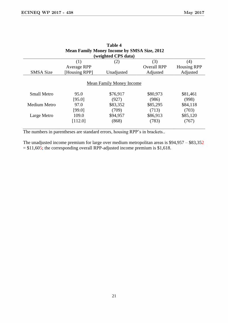
Before we begin our formal analysis, consider Table 4, where we compare the

unconditional, unadjusted family income means by metro size (column 2) to the corresponding

unconditional means adjusted by the overall RPP (column 3) and adjusted by housing prices only

(column 4). To appreciate the effect of overall RPP adjustment, note that the difference in means

between large and medium SMSAs drops from $11,604 to $1,618 after correcting for the overall

spatial price differences. If we adjust for housing prices only, the difference between the small

ECINEQ WP 2017 - 438 May 2017

14

metro and large metro areas is more compressed: $3659 in column (4) versus $5940 in column

(3).

We use the following OLS specification, which is patterned after equation (2) in Glaeser

and Mare (2001, 328),13 to formally test for agglomeration benefits:

ln(𝐼𝑛𝑐𝑜𝑚𝑒)𝑗,𝑐 = (𝐹𝐶𝑗)𝛽 + (𝑀𝑆𝑐)𝛤 + 𝜀𝑗,𝑐, (5)

where the log of money income of family j in geographical location c is a function of a vector of

family characteristics, 𝐹𝐶𝑗, that includes the number of children and characteristics of the family

head (age, sex, race, education, and previous years of full- and part-time experience). Equation

(5) also includes a vector of indicator variables, 𝑀𝑆𝑐, that measures the metro size of location c.

Specifically, equation (5) controls for metropolitan areas between 100,000 and 500,000 persons

(Small), metro areas between 500,000 and 2.5 million persons (Medium), and areas with more

than 2.5 million persons (Large). As such, the estimated vector of coefficients on metropolitan

size, 𝛤, contains the key coefficients of interest, measuring the capitalization of agglomeration

benefits into family income relative to the omitted nonmetropolitan areas.

Results for the vector of coefficients measuring metropolitan density effects from the

estimation of equation (5) are presented in Table 5.14 Column 1 of Table 5 presents results for

the nominal earnings equation and indicates that families in the smallest metropolitan areas earn

8.8 percent (with a 95 percent confidence interval of 6.2 percent to 11.3 percent) more than their

nonmetropolitan counterparts annually.15 Likewise, the families living in the Middle and Large

metropolitan areas earn 14.3 percent (95 percent confidence interval of 11.9 percent to 16.8

percent) and 25.0 percent (95 percent confidence interval of 22.1 percent to 27.9 percent) annual

income premiums relative to nonmetropolitan families, respectively. These results imply that a

nonmetropolitan family moving to the Reno, NV, Pittsburgh, PA, or Chicago, IL metropolitan

ECINEQ WP 2017 - 438 May 2017

15

statistical areas could expect an 8.8 percent, 14.3 percent, or 25.0 percent increase in family

income, respectively, on average.

Our results are largely consistent with metro-size premiums that are capitalized into

family money incomes. Specifically, the families in all the metropolitan areas are estimated to

have significantly higher incomes than the nonmetropolitan families, and the differentials are

increasing with metropolitan population density. Furthermore, formal F-tests also reject the null

hypothesis of homogeneous earnings differentials across each of the pairwise metropolitan size

categories at the 1% level, suggesting that the estimated income differentials by metropolitan

size are significantly different from one another.

Column 2 of Table 7 presents results from a similar specification using the log of real

(RPP-adjusted) family money income as the dependent variable in equation (5). Note that the

impact of metropolitan location has a positive and statistically significant impact on real income

across all metropolitan population density classifications. Our estimates imply that the families

in Metro 1 areas have 3.0% higher real incomes (95% confidence interval of 0.7% to 5.5%) and

the families in Metro 2 areas earn 5.9% more on average (95% confidence interval of 3.6% to

8.2%) than the nonmetropolitan families. These results are consistent with either agglomeration

economies or a positive sorting equilibrium, one in which workers who have higher unobserved

levels of productivity choose to live in the more densely populated areas. F-tests also reject the

null hypothesis of homogenous metropolitan effects at the 5% level.

Interestingly, however, the real income premium for the largest metropolitan

classification is estimated to be 3.6% (roughly two percentage points less than the Medium

premium).16 In terms of real income potential, a nonmetropolitan family is likely to experience

the largest gains in income, on average, by moving to a medium-sized city like Pittsburgh, PA,

ECINEQ WP 2017 - 438 May 2017

16

rather than to a small city like Reno, NV, or to a large city like Chicago, IL. These results could

reflect two effects – an agglomeration effect raising incomes and amenities reducing incomes –

working in opposite directions, with the agglomeration effect being larger when a family moves

between Small and Medium cities and smaller when it moves from Medium to Large cities.

Alternatively, there could be a worker-sorting process that is nonlinear in terms of the

unobserved productivity drivers.

Finally, Table 5 (column 3) allows us to compare a housing-price adjustment to the

overall RPP adjustment.17 With only a housing-price adjustment, small and large metro areas

offer no income premium over the nonmetro areas. Like the overall RPP adjustment, medium-

size cites provide the largest premium over the nonmetro areas, but the overall RPP premium is

about twice the housing-only premium (5.7 percent vs. 2.7 percent). These findings demonstrate

the importance of including a broader set of prices for goods and services when making spatial

price adjustments.

Conclusion

Calls for the use of spatial price indices in public policy analysis have come from such

notables as Nobel Prize winner Angus Deaton and the prestigious National Academy Panel on

Poverty and Family Assistance. The U.S. government recently produced the first-ever, official

regional price parities (RPPs) for all the metro and nonmetro areas in the country. Using these

measures, we investigate the impact of RPP adjustments on four important public policy issues:

overall and regional poverty rates, income inequality, vertical equity and tax progressivity, and

urban agglomeration premiums.

ECINEQ WP 2017 - 438 May 2017

17

We find that RPP adjustments bring regional mean incomes closer together, reduce

overall headcount poverty rates slightly (poverty rates increase in the Northeast and West, but

are offset by reductions in poverty rates in the South and Midwest), and most notably eliminate

the metro versus nonmetro poverty rate difference. They do not alter regional income inequality

rankings (higher-income families tend to live in the higher-price areas in each region); however,

the adjustments affect both overall inequality and effective federal tax progressivity. Inequality,

measured by the Gini coefficient, declines by an amount equivalent to a $1,500 cash transfer to

each U.S. primary family. Correcting for local prices increases effective tax progressivity by

more than 25 percent, or the equivalent of a $2,500 per family cash transfer.

Additionally, we use the RPPs to revisit the income premiums associated with

metropolitan areas. We find that, after adjusting for RPPs and controlling for the family head’s

characteristics, the higher family incomes found in major metropolitan areas largely, though not

completely, disappear.

ECINEQ WP 2017 - 438 May 2017

18

Table 1

Average Regional Price Parities for Selected Groups, 2012

Group RPP

U.S. Index 100.0

U.S. Primary Family Average 99.7

All Metro Area Average 101.9

Small Metro Area Average 95. 0

Medium Metro Area Average 97.4

Large Metro Area Average 109.3

Non-Metro Area Average 87.9

Honolulu Index

122.9

New York-Newark-Jersey City Index 122.2

San Jose-Sunnyvale-Santa Clara Index 122.0

Bridgeport-Stamford-Norwalk Index 121.5

Santa Cruz-Watsonville Index 121.4

Danville, VA Index 79.4

Jefferson City, MO Index 80.8

Jackson, TN Index 81.5

Jonesboro, AR Index 81.7

Rome, GA Index 82.2

Head ≥ 65 Average

99.0

Head < 65 Average 100.0

Poor Average 98.8

Income < $25,000 Average 98.5

$25,000 ≤ Income < $75,000 Average 98.6

$75,000 ≤ Income < $150,000 Average 100.3

Income ≥ $150,000 Average

104.1

Note: All RPP indices are for primary families using weighted CPS data

ECINEQ WP 2017 - 438 May 2017

19

Table 2

Summary Statistics for Income, Poverty, and Inequality by Metro Status, 2012

(weighted CPS data)

(1) (2) (3)

Geographical Area Census CPS Microdata RPP Adjusted

Mean Family Money Income

U.S. $82,843 $82,799 $82,719

(322) (403) (394)

Metro $86,892 $86,993 $81,501

($1,106) ($812) ($734)

Nonmetro $75,726 $75,801 $78,989

($838) ($640) ($654)

Poverty Rate

U.S. 0.118 0.118 0.116

(na) (0.003) (0.003)

Metro na 0.137 0.117

(0.003) (0.003)

Nonmetro na 0.114 0.116

(0.002) (0.002)

Gini Coefficient

U.S. 0.451 0.450 0.443

(0.0025) (0.0020) (0.0020)

Metro 0.453 0.452 0.447

(0.0028) (0.0023) (0.0022)

Nonmetro 0.412 0.411 0.410

(0.0050) (0.0045) (0.0043)

The numbers in parentheses are standard errors, calculated using: for weighted mean family

money incomes (SAS Proc Means), poverty rates (Bishop, Formby Zheng, 1997), and Gini

coefficients (Bishop, Formby, Zheng, 1998).

ECINEQ WP 2017 - 438 May 2017

20

Table 3

Summary Statistics for Income, Poverty, and Inequality by U.S. Census Region, 2012

(weighted CPS data)

(1) (2) (3)

Region Census CPS Microdata RPP Adjusted

Mean Family Money Income

Northeast $92,651 $92,324 $84,850

($1,498) ($1,034) ($929)

Midwest $83,194 $83,017 $88,869

($1,115) ($861) ($905)

South $75,726 $75,801 $78,989

($838) ($640) ($654)

West $86,892 $86,993 $81,501

($1,106) ($812) ($734)

Poverty Rate

Northeast 0.105 0.105 0.121

(na) (0.003) (0.003)

Midwest 0.102 0.102 0.092

(na) (0.003) (0.003)

South 0.132 0.132 0.121

(na) (0.003) (0.002)

West 0.119 0.119 0.128

(na) (0.003) (0.003)

Gini Coefficient

Northeast 0.455 0.453 0.448

(0.0062) (0.0047) (0.0046)

Midwest 0.438 0.437 0.432

(0.0059) (0.0046) (0.0046)

South 0.449 0.449 0.442

(0.0045) (0.0036) (0.0034)

West 0.454 0.455 0.449

(0.0047) (0.0034) (0.0035)

The numbers in parentheses are standard errors.

ECINEQ WP 2017 - 438 May 2017

21

Table 4

Mean Family Money Income by SMSA Size, 2012

(weighted CPS data)

(1) (2) (3) (4)

SMSA Size

Average RPP

[Housing RPP]

Unadjusted

Overall RPP

Adjusted

Housing RPP

Adjusted

Mean Family Money Income

Small Metro 95.0 $76,917 $80,973 $81,461

[95.0] (927) (986) (998)

Medium Metro 97.0 $83,352 $85,295 $84,118

[99.0] (709) (713) (703)

Large Metro 109.0 $94,957 $86,913 $85,120

[112.0] (868) (783) (767)

The numbers in parentheses are standard errors, housing RPP’s in brackets..

The unadjusted income premium for large over medium metropolitan areas is $94,957 – $83,352

= $11,605; the corresponding overall RPP-adjusted income premium is $1,618.

ECINEQ WP 2017 - 438 May 2017

22

Table 5

OLS Estimates of Agglomeration Benefits by Metro Classification

(weighted CPS data)

Estimated Coefficients

(1) (2) (3)

VARIABLES Ln(Income) Ln(RPP-

Adjusted

Income)

Ln(Housing-

Adjusted

Income)

Small Metro 0.084*** 0.030** 0.019

(0.012) (0.012) (0.012)

Medium Metro 0.134*** 0.057*** 0.027**

(0.011) (0.011) (0.011)

Large Metro 0.223*** 0.035*** -0.0006

(0.012) (0.012) (0.012)

Observations 52,041 52,041 52,041

R-squared 0.334 0.326 0.324

The numbers in parentheses are standard areas

*** p < 0.01, ** p < 0.05

ECINEQ WP 2017 - 438 May 2017

23

Table A1

Lorenz and Concentration Ordinates for U.S. Family Incomes, 2012

(weighted CPS data)

(1) (2) (3) (4) (5) (6) (7) (8) (9)

Decile 𝐿𝑥 𝐿𝑦 (2) – (1) 𝐶𝑦 (4) – (1) 𝐶𝑎𝑡 (6) – (1) Caty (8) – (1)

1 0.0105 0.0106 0.0001 0.0108 0.0003* 0.0135 0.0030* 0.0139 0.0034*

(0.0001) (0.000) (0.0001) (.0002)

2 0.0375 0.0381 0.0006* 0.0386 0.0011* 0.0464 0.0089* 0.0476 0.0101*

(0.0002) (0.0002) (0.0002) (.0003)

3 0.0770 0.0785 0.0015* 0.0794 0.0024* 0.0918 0.0148* .0944 0.0174*

(0.0002) (0.0003) (0.0002) (.0005)

4 0.1298 0.1323 0.0025* 0.1337 0.0039* 0.1499 0.0202* 0.1542 0.0244*

(0.0003) (0.0004) (0.0003) (.0006)

5 0.1970 0.2009 0.0039* 0.2027 0.0057* 0.2218 0.0248* 0.2278 0.0308*

(0.0004) (0.0005) (0.0003) (.0007)

6 0.2806 0.2861 0.0055* 0.2885 0.0079* 0.3093 0.0287* 0.3173 0.0367*

(0.0004) (0.0006) (0.0003) (.0007)

7 0.3834 0.3904 0.0069* 0.3933 0.0099* 0.4152 0.0318* 0.4251 0.0417*

(0.0005) (0.0007) (0.0004) (.0010)

8 0.5112 0.5192 0.0080* 0.5223 0.0111* 0.5442 0.0329* 0.5550 0.0437*

(0.0005) (0.0007) (0.0005) (.0011)

9 0.7777 0.6853 0.0076 0.6880 0.0103* 0.7085 0.0308* 0.7182 0.0405*

(0.0041) (0.0049) (0.0045) (.0050)

Note: 𝐿𝑥 is the Lorenz curve for family incomes, 𝐿𝑦 is the Lorenz curve for RPP-adjusted

incomes, 𝐶𝑦 is the concentration curve for RPP-adjusted incomes ordered by unadjusted incomes

(𝑥), 𝐶𝑎𝑡 is the concentration curve for (family income – federal taxes) ordered by 𝑥, and 𝐶𝑎𝑡𝑦 is

the concentration curve for (family income – federal taxes)/ RPP ordered by 𝑥.

Standard errors are from Bishop, Chow, and Formby (1994).

ECINEQ WP 2017 - 438 May 2017

24

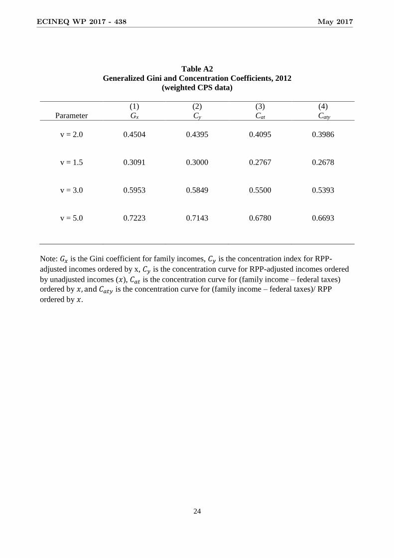
Table A2

Generalized Gini and Concentration Coefficients, 2012

(weighted CPS data)

(1) (2) (3) (4)

Parameter Gx Cy Cat Caty

v = 2.0

0.4504

0.4395

0.4095

0.3986

v = 1.5 0.3091 0.3000 0.2767 0.2678

v = 3.0 0.5953 0.5849 0.5500 0.5393

v = 5.0 0.7223 0.7143 0.6780 0.6693

Note: 𝐺𝑥 is the Gini coefficient for family incomes, 𝐶𝑦 is the concentration index for RPP-

adjusted incomes ordered by x, 𝐶𝑦 is the concentration curve for RPP-adjusted incomes ordered

by unadjusted incomes (𝑥), 𝐶𝑎𝑡 is the concentration curve for (family income – federal taxes)

ordered by 𝑥, and 𝐶𝑎𝑡𝑦 is the concentration curve for (family income – federal taxes)/ RPP

ordered by 𝑥.

ECINEQ WP 2017 - 438 May 2017

25

Table A3

Full Summary Statistics and OLS Estimates for the Agglomeration Analysis

(weighted CPS data)

Estimated Coeff. (Std. Error)

(1) (2) (3) (4)

VARIABLES Summary Statistics

(Std. Dev.)

Ln(Income) Ln(RPP Adj.

Income)

Ln(Housing Adj.

Income)

Small Metro 0.173 0.084*** 0.030** 0.019

(0.378) (0.012) (0.012) (0.012)

Medium Metro 0.270 0.134*** 0.057*** 0.027**

(0.444) (0.011) (0.011) (0.011)

Large Metro 0.359 0.223*** 0.035*** -0.001

(0.480) (0.012) (0.012) (0.012)

Number of Children 1.066 0.006* 0.005 0.005

(1.181) (0.004) (0.004) (0.004)

Age 49.330 0.011*** 0.011*** 0.010***

(15.661) (0.000) (0.000) (0.000)

Full-time Experience 28.017 0.016*** 0.016*** 0.016***

(24.647) (0.000) (0.000) (0.000)

Part-time 4.733 0.009*** 0.008*** 0.008***

Experience (13.996) (0.000) (0.000) (0.000)

Male 0.527 0.085*** 0.087*** 0.087***

(0.499) (0.008) (0.008) (0.008)

High School Grad. 0.464 0.332*** 0.328*** 0.327***

(0.499) (0.015) (0.015) (0.015)

Associates Degree 0.104 0.505*** 0.499*** 0.494***

(0.306) (0.018) (0.018) (0.018)

Bachelors Degree 0.202 0.793*** 0.780*** 0.775***

(0.402) (0.016) (0.016) (0.016)

Masters/Ph.D. 0.122 0.967*** 0.948*** 0.942***

(0.327) (0.018) (0.018) (0.018)

Hispanic 0.146 -0.266*** -0.286*** -0.295***

(0.353) (0.012) (0.012) (0.012)

Black 0.120 -0.392*** -0.386*** -0.382***

(0.324) (0.013) (0.013) (0.013)

Asian 0.051 -0.100*** -0.146*** -0.162***

(0.220) (0.019) (0.019) (0.019)

Other Race 0.028 -0.198*** -0.212*** -0.218***

(0.164) (0.027) (0.027) (0.027)

Constant 9.376*** 9.506*** 9.530***

(0.028) (0.028) (0.028)

Observations 52,041 52,041 52,041

R-squared 0.334 0.326 0.324

Standard errors in parentheses

*** p<0.01, ** p<0.05, * p<0.1

ECINEQ WP 2017 - 438 May 2017

26

Endnotes

1 Carrillo, Early, and Olsen (2014) have also published unofficial price indices covering all

produced goods and services in all areas of the U.S. (metro and nonmetro) that extend back to

1982.

2 For previous studies of the consequences of spatial price adjustments for U.S. poverty, see

Nelson and Short (2003), Nelson (2004), Dalaker (2005), Jolliffe (2006), Beth Curran, et al.

(2006), Renwick (2009), and Early and Olsen (2012). Most of these studies compare poverty

rates across the four Census regions, the 50 U.S. states, or the 98 central cities with adjustments

for housing prices. Only the last study considers variation in other prices, and it finds little

difference in poverty rates by metropolitan status. To our knowledge, our paper is the first to

examine the consequences of spatial price adjustment for income inequality and tax

progressivity.

3 The Supplemental Poverty Measure (Short 2015) corrects for differences in housing costs only.

Renwick et al. (2014) and Bishop, Lee, and Zeager (2017) replace housing costs with RPPs in

the construction of the Supplemental Poverty Measure.

4 To show the importance the U.S. Census placed on the new RPPs, U.S. Secretary of

Commerce, Penny Pritzker (Bureau of Economic Analysis 2014, 1) said, “For the first time,

Americans looking to move or take a job anywhere in the country can compare inflation-adjusted

incomes across the states and metropolitan areas to better understand how their personal income

may be affected by a job change or move…”.

5 Aten, Figueroa, and Martin (2011) and Aten and Figueroa (2014) provide a detailed overview

of the BEA’s newly constructed RPPs. Except where otherwise noted, this discussion relies

heavily on their documentation.

ECINEQ WP 2017 - 438 May 2017

27

6 Table 1 also provides the RPPs for the five lowest and five highest SMSAs.

7 We replicated much of the analysis with adult equivalent comprehensive household income

(including taxes and in-kind transfers such as food stamps) and obtained essentially the same

results as reported below. See Bishop, Formby and Zheng (1998) for a definition of adult

equivalent comprehensive household income.

8 Appendix Table A1, columns (1) and (2), provide the family money income Lorenz ordinates

by decile, before and after RPP adjustment.

9 We also made similar adjustments in poverty rates for racial minorities. Recall from Table 1

that the RPPs for Asians and Hispanics are above the U.S. average. RPP adjustments increase

the Hispanic poverty rate from 23.4 percent to 24.3 percent and the Asian poverty rate from 9.3

percent to 10.3 percent.

10 For a standard treatment of these issues, including tax progressivity, see Lambert (1989). The

following analysis is based on the standard Gini coefficients, however, we report the underlying

decile Lorenz and concentration ordinates in Appendix Table A1 and some generalized Gini

coefficients in Table A2.

11 We obtain a re-ranking effect of 𝐶𝑦 − 𝐺𝑦 = 0.4395 − 0.4128 = 0.0267.

12 The change in vertical equity in the federal tax system due to RPP adjustment is similar in

magnitude to the effect of tax noncompliance; see Bishop, Formby, and Lambert (2000).

13 We adapt their specification by using incomes in places of wages and dropping the time

dimension and the fixed-effects term, which we cannot estimate with CPS data. Many of their

results also constrain this term to be zero (Glaeser and Mare 2001, 328).

14 The full set of results, along with summary statistics from the estimation of equation (5), are

provided in Appendix Table A3.

ECINEQ WP 2017 - 438 May 2017

28

15 We calculate the percentage earnings differentials using the method of Holversen and

Palmquist (1980).

16 F-tests for the equality of the coefficients on Metro 1 and Metro 3 fail to reject the null

hypothesis that these coefficients are statistically indistinguishable at any conventional level of

significance.

17 The housing index (𝑅𝑃𝑃𝐻) is constructed as 𝑅𝑃𝑃𝐻 = (0.41)𝐵𝐸𝐴𝐻 + (0.59)100, where

𝐵𝐸𝐴𝐻 is the housing component of the BEA’s overall RPP. The weights 0.41 and .059 come

from the 2013 CPI weights for housing and other goods, respectively. That is, we are assuming

for this particular exercise that only housing prices differ across regions; all other prices are at

the national average (100).

References

Albouy, David. 2009. The unequal geographic burden of federal taxation. Journal of Political

Economy 117 (4): 635-67.

Aten, Bettina H., Eric B. Figueroa, Troy M. Martin. 2011. Regional price parities by expenditure

class for 2005-2009. Survey of Current Business 91 (May), 73–87.

Aten, Bettina H., and Eric B. Figueroa. 2014. Real personal income and regional price parities

for states and metropolitan areas 2008-2012. Survey of Current Business 94 (June): 1–9.

Atkinson, Anthony B. 2003. Income inequality in OECD countries: Data and explanations.

CESifo Economic Studies 49 (4): 479-513.

Beth Curran, Leah, Harold Wolman, Edward W. Hill, and Kimberly Furdell. 2006. Economic

well-being and where we live: Accounting for geographical cost-of-living differences in

the U.S. Urban Studies 43 (13): 2443-2466.

ECINEQ WP 2017 - 438 May 2017

29

Bishop, John A. K. Victor Chow, and John P. Formby. 1994. Testing for marginal changes in

income distributions with Lorenz and concentration curves. International Economic

Review 35 (2): 479-488.

Bishop, John A., John P. Formby, and Peter Lambert. 2000. Redistribution through the income

tax: The vertical and horizontal effects of noncompliance and tax evasion. Public

Finance Review 28 (4): 335-350.

Bishop, John A., John P. Formby, and Paul D. Thistle. 1992. Convergence of the South and non-

South income distributions 1969-1979. American Economic Review 82 (1): 262-272.

Bishop, John A., John P. Formby, and Paul D. Thistle. 1994. Convergence and divergence of

regional income distributions and welfare. Review of Economics and Statistics 76 (2):

228-235.

Bishop, John .A., John P. Formby, and Buhong Zheng. 1997. Statistical inference and the Sen

index of poverty. International Economic Review 38 (2): 381-387.

Bishop, John A., John P. Formby, and Buhong Zheng. 1998. Distribution sensitive measures of

poverty in the United States. Review of Social Economy 57 (3): 306-343.

Bishop, John A., Jonathan Lee, and Lester A. Zeager. 2017. Improving the supplemental poverty

measure: Two proposals. Society for the Study of Economic Inequality (ECINEQ)

Working Paper 2017-429.

Bureau of Economic Analysis. 2014. News Release, U.S. Department of Commerce, April 24.

Bureau of Labor Statistics. 1979. Three Budgets for an Urban Family of Four Persons, 1969-70.

Washington, DC: U.S. Government Printing Office.

Carrillo, Paul E., Dirk W. Early, and Edgar O. Olsen. 2014. A panel of interarea price indices for

all areas of the United States 1982-2012. Journal of Housing Economics 26 (C), 81-93.

ECINEQ WP 2017 - 438 May 2017

30

Citro, Constance.F., and Robert T. Michael, ed. 1995. Measuring Poverty: A New Approach.

National Academy Press, Washington, DC.

Combes, Pierre-Phillippe, Duranton Gilles, and Laurent Gobillon. 2008. Spatial wage disparities:

Sorting matters! Journal of Urban Economics 63 (2): 723-742.

Dalaker, Joe. 2005. Alternative poverty estimates in the United States: 2003. Current Population

Reports, June, 1-22.

Deaton, Angus. 2010. Price indexes, inequality, and the measurement of world poverty.

American Economic Review 100 (1): 3-34.

Deaton, Angus. 2016. Measuring and understanding behavior, welfare, and poverty. American

Economic Review 106 (6): 1221-1243.

Deaton, Angus., and Dupriez, O. 2011. Spatial price differences within large countries.

Unpublished Paper, June.

Early, Dirk W., and Edgar O. Olsen. 2012. Geographical price variation, housing assistance and

poverty, In The Oxford Handbook of the Economics of Poverty, Jefferson Philip N. ed.

380-424. Oxford: Oxford University Press.

Glaeser, Eward L., and Joshua D. Gottlieb. 2009. The wealth of cities: Agglomeration economies

and spatial equilibrium in the United States, Journal of Economic Literature 47 (4): 983-

1028.

Glaeser, Edward L., and David C. Mare. 2001. Cities and skills, Journal of Labor Economics 19

(2): 316-342.

Glaeser, Edward L., and Matthew G. Resseger. 2010. The complementarity between cities and

skills. Journal of Regional Science 50 (1): 221-244.

ECINEQ WP 2017 - 438 May 2017

31

Holverson, Robert, and Raymond Palmquist. 1980. The interpretation of dummy variables in

semilogarithmic equations. American Economic Review 70 (3): 474-5.

Jolliffe, Dean. 2006. Poverty, prices, and place: How sensitive is the spatial distribution of

poverty to cost of living adjustments? Economic Inquiry 44 (2): 296-310.

Lambert, Peter J. 1989. The Distribution and Redistribution of Income – A Mathematical

Analysis. Oxford, England: Basil Blackwell.

Nelson, Charles. 2004. Geographic Adjustments in Poverty Thresholds. Washington, DC:

Census Bureau, http://citeseerx.ist.psu.edu/viewdoc/summary?doi=10.1.1.207.4251.

Nelson, Charles, and Kathleen Short, 2003. The Distributional Implications of Geographic

Adjustment of Poverty Thresholds, Washington, DC: Census Bureau,

https://www.census.gov/hhes/povmeas/publications/povthres/geopaper.pdf.

Puga, Diego. 2010. The magnitude and causes of agglomeration economies. Journal of Regional

Science 50 (1): 203-219.

Renwick, Trudi. 2009. Alternative geographic adjustments of U.S. poverty thresholds: Impact on

state poverty rates. Washington, DC: Census Bureau.

Renwick, Trudi, Bettina Aten, Eric Figueroa, and Troy Martin. 2014. Supplemental poverty

measure: A comparison of geographic adjustments with regional price parities vs. median

rents from the American Community Survey. Washington, DC: Census Bureau, Social,

Economic and Housing Statistics Division Working Paper No. 2014-22.

Roback, Jennifer. 1982. Wages, rents, and the quality of life. The Journal of Political Economy

90 (6): 1257-1278.

Short, Kathleen. 2015. The supplemental poverty measure: 2014, Washington. DC. Census

Bureau, Current Population Reports, P60-254.

ECINEQ WP 2017 - 438 May 2017