Incorporating Topological Constraints within Interactive Segmentation andContour Completion via Discrete Calculus∗

Jia Xu Maxwell D. Collins Vikas SinghUniversity of Wisconsin-Madison

http://pages.cs.wisc.edu/˜jiaxu/projects/euler-seg/

Abstract

We study the problem of interactive segmentation andcontour completion for multiple objects. The form of con-straints our model incorporates are those coming from userscribbles (interior or exterior constraints) as well as infor-mation regarding the topology of the 2-D space after par-titioning (number of closed contours desired). We discusshow concepts from discrete calculus and a simple identityusing the Euler characteristic of a planar graph can be uti-lized to derive a practical algorithm for this problem. Wealso present specialized branch and bound methods for thecase of single contour completion under such constraints.On an extensive dataset of ∼ 1000 images, our experi-ments suggest that a small amount of side knowledge cangive strong improvements over fully unsupervised contourcompletion methods. We show that by interpreting user in-dications topologically, user effort is substantially reduced.

1. Introduction

This paper is focused on developing optimizationmodels for the problem of multiple contour comple-tion/segmentation subject to side constraints. The type ofconstraints our algorithm incorporates are (a) those relatingto inside (or outside) seed indications given via user scrib-bles; (b) global constraints on the topology, i.e., informationwhich reflects the number of unique closed contours a useris looking for. Given the output from a boundary detec-tor (e.g., Probability of Boundary or Pb [25]), we obtain alarge set of weighted locally-based contours (or edgelets) asshown in Fig. 1. The objective then is to find k closed “le-gal” contour cycles with desirable properties (e.g., curvilin-ear continuity, strong edge gradient, small curvature), wherelegal solutions are those that satisfy the side constraints,shown in Fig. 1. The basic primitives in our constructionare contour fragments, not pixels. The motivation for thischoice is similar to most works on contour detection for im-

∗This is a extended-CVPR version, dated May 1, 2013, with detailedoptimization schemes and more experimental results.

age segmentation – by moving from predominantly region-based terms to a function that utilizes strength of edges, weseek to partly mitigate the dependence of the final segmen-tation on the homogeneity of the regions alone and the num-ber of seeds. Additionally, in at least some circumstances,one expects benefits in terms of running time by utilizing afew hundred edges instead of a million pixels in the image.Our high level goal is the design of practical contour com-pletion algorithms that take advice – which in a sense paral-lels a powerful suite of methods that have recently demon-strated how global knowledge can be incorporated withinpopular region-based image segmentation methods [26].

Figure 1: Left to right: input images, edgelets or contours withseed indications, and final contour. Foreground is marked in green;background is marked in red; boundrary is marked in white. Bestviewed in color.Related Work. The study of methods for detection ofsalient edges and object boundaries from images has a longhistory in computer vision [37]. The associated body ofliterature is vast – methods range from performing edge de-tection at the level of local patches [32], to taking the conti-nuity of edge contours into account [37, 29], to incorporat-ing high-level cues [36] such as those derived from shapeand/or appearance [25]. While the appropriateness of a spe-cific contour detector is governed by the downstream appli-cation, developments in recent years have given a numberof powerful methods that yield high quality boundary detec-tion on a large variety of images and perform well on estab-lished benchmarks [25]. Broadly, this class of methods useslocal measurements to estimate the likelihood of a boundaryat a pixel location. To do this, the conventional approachwas to identify discontinuities in the brightness channel,

1

where as newer methods exploit significantly more infor-mation. For instance, [27] suggests a logistic regression onbrightness, color, and texture, and [9, 24] learns a classifierby operating on a large number of features derived from im-age patches or filter responses at multiple orientations. Con-temporary to this line of research, there are also a variety ofexisting algorithms that integrate (or group) local edge in-formation into a globally salient contour. Since one expectsthe global contour to be smooth, the well known Snakes for-mulation introduced an objective function based on first andsecond derivative of the curve. Others have proposed utiliz-ing the ratio of two line integrals [18], incorporating curva-ture [31, 10], joining pre-extracted line segments [40, 35],and using CRFs to ensure the continuity of contours [30].Note that despite similarities, contour detection on its ownis not the same as image segmentation. In fact, even whenformalized under contour completion, an algorithm may notalways produce a closed contour. Nonetheless, from most“edge-based” methods one can obtain a partition of the im-age into object and background regions. Without gettinginto the merits of edges versus regions, one can view edge-based contours as a viable alternative to “region-based” im-age segmentation methods in many applications.

The success of the above developments notwithstanding,the applicability of these methods has been somewhat lim-ited by their inability to successfully discriminate betweencontours of different classes of objects. To address this lim-itation, there has been a noticeable shift recently towardsthe incorporation of additional information within the con-tour completion process. In particular, several groups havepresented frameworks that leverage category specific (or se-mantic) information into the process of obtaining closed ob-ject boundaries. Specific examples of this line of work in-clude semantic contours [16], the hierarchical ultrametriccontour map [2], and particle filtering based object detec-tion via edges [23]. The basic idea here is to achieve abalance between bottom up edge/boundary detection andtop-down supervision, for simultaneous image segmenta-tion and recognition. While semantic knowledge based con-tour completion is quite powerful, its performance invari-ably depends on the richness of the underlying training cor-pus. Indeed, if the shape epitomes do not reflect the objectof interest accurately enough (significant pose variations),if there is clutter/occlusion, or when a novel class is notwell represented in the training data, the results may beunsatisfactory. In these circumstances, it seems natural toendow the contour completion models with the capabilityto leverage some form of user supervision (foreground andbackground seeds) [15]. Further, knowledge provided in theform of the number of closed contours a user requires, canbe a powerful form of user guidance as well. Notice thatthe adoption of Grabcut type methods suggests that a nom-inal amount of “interactive scribbles” is readily available in

many applications, and may significantly improve the qual-ity of solutions. While there are many mechanisms whichincorporate such constraints in region based segmentation,only a few methods take such information explicitly intoaccount for edge-based contour completion. In this work,we leverage a discrete calculus based toolset to incorpo-rate such topological and seed indications type supervisionwithin a practical contour completion algorithm.

The primary contributions of the this paper are: (i) Wepresent a unified optimization model for multiple con-tour completion/segmentation which incorporates topologi-cal constraints as well as inclusion/exclusion of foregroundand background seeds. The topological knowledge is in-cluded by using the Euler characteristic of the edgeletgraph where as inclusion/exclusion constraints utilize con-cepts from discrete calculus. (ii) For an extensive dataset,we provide strong evidence that with a small amount ofuser interaction, one can obtain high quality segmentationsbased on edge contours information alone. We give aneasy to use implementation, as well as user scribble datacorresponding to varying levels of interaction on this large(∼ 1000) set of images.

2. PreliminariesThe tools of discrete calculus provide a powerful formal-

ism to represent the topological information in an image[14, 20, 7]. We use conventions of discrete calculus to de-scribe our problem of finding multiple contour closures. Inthis section, we introduce the idea of cell complices whichare the fundamental building blocks of our construction.The following text also introduces the necessary notations,which will be used thoughout the rest of the text.

2.1. Discrete Calculus

The domain of an image is decomposed into a set ofcells. If the decomposition is such that (i) the interiors ofthe cells are disjoint and (ii) the boundary between any twop-dimensional cells is a (p − 1)-dimensional cell then wehave a cell complex. As an example, consider a planar graphG = 〈V,E, F 〉with vertices V , edgesE, and faces F . Sucha graph has incidence relationship between each face andits bounding edges, and between each edge and its endpointvertices. Similarly, each vertex is incident on two or moreedges and each edge is incident on two faces. Notice thatthe interior of a pair of faces is disjoint, and the boundarybetween any two faces gives an edge, where the dimensionis reduced by one. As a consequence, we get a 2D cellcomplex for a planar graph, and also a set of incidence rela-tionships among simplices of different dimensions.

A cell complex may be oriented such that we can de-scribe directions on each cell relative to its orientation, seeFig. 2(a). Each type of cell has a corresponding pair ofpossible orientations: a vertex (0-cell) is either a source or

Vertex Edge Face Coherent Anti-coherent

(a) (b)Figure 2: Visualization of the orientations on cells of different dimen-sionalities (a). In (b) we show in the left column p-cells with all of theirboundary (p − 1)-cells coherently oriented, and all boundary cells anti-coherently oriented in the right column.

Node Edge Face

Primal

Dual

Figure 3: Duality relationships between 2D cell complices.

a sink while an edge (1-cell) may be directed toward eitherendpoint. Further, each cell induces a corresponding ori-entation on incident cells; for example, a directed edge hasa source endpoint vertex at one end and sink at the other.The orientations of a cell and a member of its boundary arecoherent if the induced orientations agree, an example isshown in Fig. 2(b).

We may represent the two-dimensional image as an ori-ented complex. All faces are given the same orientation,while edges and vertices are given arbitrary orientations.After enumerating its constituent vertices, edges and faces,a selection of some subset of faces is specified with an in-dicator vector x ∈ {0, 1}|F |. xi = 1 denotes the candidateface Fi ∈ F is in the foreground, and xi = 0 otherwise.Similarly, we represent the edge and vertex configuration ofG by indicator vectors y ∈ {0, 1}|E| and z ∈ {0, 1}|V | re-spectively. We require that the indicator vectors x,y, z oneach level of cell consistently describe a segmentation. Thekey relationship is consistency between the labels on theincident cells. These relationships can be expressed alge-braically using the notion of a dimension-appropriate inci-dence matrix. The edge-face incidence matrix (also calledthe boundary operator) C1 ∈ {−1, 0, 1}|E|×|F | is definedby

C1;ij =

1 if edge i is incident to face j and coherently oriented;−1 if edge i is incident to face j and anti-coherently oriented;0 otherwise.

(1)

Here, C1;ij refers to entry (i, j) in C1. Similarly,by discarding orientation information, we can define theedge-face corresponding matrix C2 ∈ {0, 1}|E|×|F | whichlabels which edges are incident to which face. It canbe calculated as the element-wise absolute value of C1,

such that C2;ij = |C1;ij |. The node-edge incident ma-trix A1 ∈ {−1, 0, 1}|V |×|E| is defined analogously to (1),where A1;ij = 1 iff node i is incident to edge j. Aswith C2, we define the node-edge corresponding matrixA2 = |A1| ∈ {0, 1}|V |×|E|. We further use a node-edge de-gree matrix A3 ∈ R|V |×|E|, where A3;ij = A2;ij/di wheredi denotes the degree of node i.

Discrete calculus describes the notion of duality betweencell complices. In a p-complex, each q-cell will have a cor-responding dual (p−q)-cell (say, q ≤ p). For any given cellcomplex, we can construct its dual in a way that preservesincidence relationships between cells, see Fig. 3. Usingthese concepts, in the following sections, we will formalizethe required constraints within a contour completion objec-tive function.

3. Problem FormulationAs described in Section 2.1, our model works with se-

lections of the cells constituting the foreground. Since thenotion of foreground for a face is self-evident, we will de-scribe the labeling of vertices and edges, starting from a facelabeling x. We enforce the following condition:

Condition 1. A p-cell is in the foreground if and only if itis incident to a (p+ 1)-cell in the foreground.

This condition ensures that each connected componentof the foreground is itself a cell complex, a property we willuse shortly.

First, we introduce an auxiliary indicator variable w ∈{0, 1}|E| which selects the boundary edges. These edgesare those which are incident to both a foreground and abackground face. W.l.o.g., consider edge 1 incident to faces1 and 2 respectively, then w1 = |x1 − x2| = I(x1 6= x2).Taken together, the full set of boundary edges precisely rep-resent the contour of the selected foreground. We can nowuse the boundary operator from Section 2.1 to derive theidentity

w = |C1x| (2)

Observe that each edge is incident to exactly two faces,and we specified that all faces have identical orientation. Itfollows that an edge must be coherent with one face andanti-coherent with the other. Therefore, for all internaledges (non-boundary edges in the foreground) the C1 oper-ator when multiplied with x, cancels the contribution fromthese two faces, leaving non-zero values only for the bound-ary edges. The internal edges (which are incident to fore-ground faces on both sides) can still be computed in a dif-ferent manner. The vector C2x will count the inside edgestwice and the boundary edges once, as we discard orienta-tion (and thus sign information). In the preceding, w.l.o.g.(C2x)1 = x1 + x2. Thus, Condition 1 will be satisfied ifthe following identity holds:

2y = w + C2x (3)

Figure 4: A superpixel-based segmentation with the foreground subgraphconsistent under condition 1. Selected faces are shaded, foreground edgesare bold and foreground vertices highlighted in yellow. Internal edgesyi 6= wi = 0 are bold/black, boundary edges yi = wi = 1 are red.

We use the matrices A2, A3 for a pair of linear inequali-ties which are equivalent to Condition 1 for vertices. Ob-serve that the vector A2y will be the number of foregroundedges incident to each foreground vertex (or node), where(A2y)i is the number of foreground edges incident to ver-tex (or node) i. Similarily, when scaled by the degree diof vertex i, (A3y)i ∈ [0, 1] will be the proportion of edgesincident to i which are in foreground. Enforcing condition1 is equivalent to:

A3y ≤ z ≤ A2y (4)

Since zi ∈ {0, 1}, the condition, zi ≥ (A3y)i, will be trueonly for zi = 1 if any edge incident to i is in foreground.Conversely, if no edge incident to i is selected in the solu-tion, then (A2y)i = (A3y)i = 0 and (4) is satisfied onlyfor zi = 0.

The expressions introduced above allow the identifica-tion of whether a user provided seed falls “inside” or “out-side” the contour completion given by w, and will serveas constraints for our multiple contour completion model.Fig. 4 shows an illustrative example for an image, wherethe input to the contour completion are edgelets (or edgels)obtained from boundaries of a globalPb derived superpixels.

Euler Characteristic. Our final requirement is to beable to specify the number of closed contours desired. Theexisting literature on region based image segmentation pro-vides some ideas on how this can be accomplished for ran-dom field based models – in the form of so-called connect-edness constraints. TopologyCuts is an extension of graph-cuts and utilizes certain levelset ideas to preserve topology[41]. The DijkstraGC [38] finds a segmentation where twomanually indicated seed points are connected via the fore-ground where as Nowozin [28] makes use of a LP relax-ation. Very recently, [8] proposed selectively perturbingthe energy function to ensure topological properties. Here,we show how a much simpler form can capture the desiredtopological properties, as described next.

For any graph we can define the Euler characteristic as

χ = |V | − |E|+ |F |, (5)

where χ = 2 for any planar embedding of a graph. Ifwe explicitly constrain that the Euler characteristic of an in-duced subgraph created by selecting any given foreground

is exactly two, this will give a foreground region that isconnected and simple in a geometric sense. For multipleconnected regions, we can use the generalized form of thisformula for arbitrary planar graphs:

|F |+ |V | − |E| = n+ 1 (6)

where n is the number of connected components.)

Lemma 3.1. Let x,y, z denote indicator vectors for the se-lection of faces, edges, and vertices for planar graph G.The selected subgraph will satisfy (6) if∑

i

xi +∑k

zk −∑j

yj = n (7)

Proof. (Sketch) The left-hand side of this formula countseach relevant quantity for the Euler characteristic of the se-lected subgraph, but it neglects to count the “outside” face.Subtract one from the RHS and derive the equality.

This will not count the extra outside faces correspondingto any “holes”. This was not a problem in our experiments,but can be explicitly avoided by requiring the backgroundbe connected using the spanning tree constraints of [33].Using (7) as a constraint in our model will guarantee thatwe recover n simply connected foregrounds.

3.1. Optimization Model

Before we introduce the contour completion model, webriefly describe the procedure for deriving the componentsof the graph from an image. This process follows exist-ing algorithms for contour and boundary detection. First,we run the globalPb detector on an image which providesthe probability of boundary for each image pixel. Next, wegenerate a set of superpixels from the image using the glob-alPb output in conjunction with TurboPixels (which useslocal information and compactness). Each superpixel cor-responds to a face, and the boundary of the superpixel cor-responds to edges in the graph (these are the basic primi-tives of the closed contours we will derive). If two edgesare connected, we introduce a node in the graph. With thisconstruction, the problem of finding multiple contour clo-sures reduces to finding multiple cycles in the graph. To se-lect the cycles for the strongest contours, we want to weightthe edges appropriately. For this purpose, we calculate twotypes of weight measures following [21]. The first, denotedby N, measures the “goodness” of edges. The better edge iis, the smaller Ni will be. The second, denoted by D, is thecount of all the pixels on the superpixel boundary. We usean objective function which is the ratio of these quantities,N(w)D(w) . This ends up being the portion of contour w.r.t arc-length which does not lie on a true image edge. Minimizingthis quantity has been shown to provide a contour that hasstrong edge support in the image.

Finally, the user indictations are represented in terms ofindicator vectors x0,x1, where x0;i = 1 if face i contains

a background seed. With the basic components (or con-straints) in hand, we now have the main optimization model.

minw,x,y,z

NTw

DTw,

s.t. w = |C1x|, 2y = w + C2x, (8a,b)

A3y ≤ z ≤ A2y, 1Tx+ 1T z− 1Ty = n, (8c,d)

x1 ≤ x ≤ 1− x0, w,x,y, z ∈ {0, 1}. (8e,f)

3.2. Optimizing Ratio Objective

Since the objective in (8) of the main paper is in ratioform, we transform it into a linear function with a free vari-able, t. Our linear ratio cost objective function is solvedby minimizing f(t,u) = (N − tD)Tu, over admissible ufor a sequence of chosen values of t. Here, u denotes theconcatenated vector of all indicator variables in the model.Assume D ≥ 0 and DTu 6= 0. For an initial finitebounding interval [tl, tu], let t0 be the initial value. Letu = arg minu f(t0,u), the procedure proceeds as follows:

• f(t0, u) = 0: NT u/DT u = t0, stop with solution t0

• f(t0, u) < 0: NT u/DT u < t0, tu ← NT u/DT u

• f(t0, u) > 0: NT u/DT u > t0, tl ← t0

Each iteration is easily solved in a few seconds using theCPLEX IP solver on a standard workstation.

3.3. Spanning Tree Constraint

In Section 3 of the main paper, we stated that the∑

i xiterm in (7) will not count the “outside” faces. In addition, itdoes not count faces introduced due to holes in the selectedforeground. If we denote the number of such holes by H ,then the actual number of faces of the foreground subgraphis∑

i xi + H + 1. Modifying the expression to match (6),this takes the form(∑

i

xi +H + 1

)+∑k

zk −∑j

yj = C + 1

∑i

xi +∑k

zk −∑j

yj = C −H(9)

where C is the number of connected components. Thereremains a small ambiguity in the constraint, such that intro-ducing a new connected component along with a new holewill maintain the equality. This can be easily eliminatedeither via a choice of objective which favors minimum arclength (and thus will avoid holes), or by explicitly restrictingH = 0.

If the background faces form one connected component,there are no holes inside the selected foreground cycles,This is acchievable with the constraints of [33] to requirethe existence of a spanning tree on the dual graph of unse-lected faces.

Denote x = 1 − x as the faces we did not select inour solution. We introduce auxiliary variables for a face-simultaneous-selection matrix S, and variable T indicatingwhich dual edges are in the spanning tree.

Sij =

{1 if xi = xj = 1, faces i and j adjacent;0 otherwise.

(10)

The spanning tree is constructed from S using the followingconstraints.

First, if Sij = 0, this cannot be an edge in the tree.

Tij ≤ Sij ∀ i, j (11)

Second, if xi = 1, there must be at least one edge incidenton face i ∑

j∼iTij ≥ xi ∀i (12)

All the background faces should form a tree. A graph is atree only if it has one fewer edge than faces∑

i∼jTij =

∑i

xi − 1 (13)

Finally, one eliminates cycles by ensuring all subsets offaces are no more connected than a tree∑

i∼j;i,j∈STij ≤

∑i∈S

xi − 1 ∀ S ⊂ F (14)

this is enforced for all subsets S of faces. If a feasible Texists, then the background must be connected and thereare no holes in the foreground. We do not use (14) in oursolver, and present it for theoretical completeness. Instead,we rely in practice on the tendency of our model’s objectiveto prefer short, simple boundaries which do not introduceunnecessary holes.

4. Beyond Superpixel-derived EdgeletsRecall that the model in Section 3.1 constructs a cell

complex using a superpixel decomposition of the image do-main. While fast algorithms for finding this decompositionare available [22], it is known that superpixels are not ro-bust for all types of images. Occlusion or weak boundariesgive cases where the set of superpixel boundary primitives(the input to our optimization) do not include some validedgelets (ones which have not been picked up by either thecontour detector or superpixel method). The natural solu-tion to this is to supplement the basic set of edgelet prim-itives with additional contour pieces that bridge the ‘gaps’and allow a more accurate contour closure even in the pres-ence of very weak signal variations. Next, we present suchan extension to find completions using a base set of discon-nected edgelets. But introducing completions between all

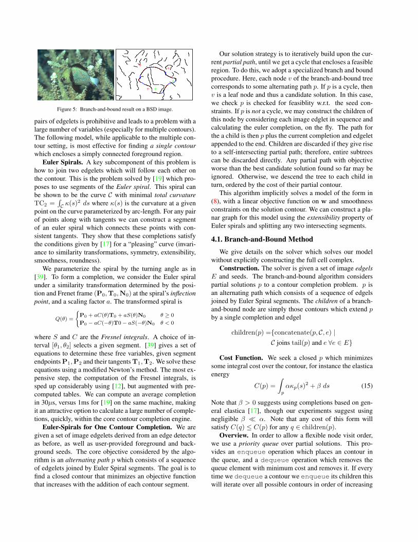
Figure 5: Branch-and-bound result on a BSD image.

pairs of edgelets is prohibitive and leads to a problem with alarge number of variables (especially for multiple contours).The following model, while applicable to the multiple con-tour setting, is most effective for finding a single contourwhich encloses a simply connected foreground region.

Euler Spirals. A key subcomponent of this problem ishow to join two edgelets which will follow each other onthe contour. This is the problem solved by [19] which pro-poses to use segments of the Euler spiral. This spiral canbe shown to be the curve C with minimal total curvatureTC2 =

∫C κ(s)2 ds where κ(s) is the curvature at a given

point on the curve parameterized by arc-length. For any pairof points along with tangents we can construct a segmentof an euler spiral which connects these points with con-sistent tangents. They show that these completions satisfythe conditions given by [17] for a “pleasing” curve (invari-ance to similarity transformations, symmetry, extensibility,smoothness, roundness).

We parameterize the spiral by the turning angle as in[39]. To form a completion, we consider the Euler spiralunder a similarity transformation determined by the posi-tion and Frenet frame (P0,T0,N0) at the spiral’s inflectionpoint, and a scaling factor a. The transformed spiral is

Q(θ) =

{P0 + aC(θ)T0 + aS(θ)N0 θ ≥ 0

P0 − aC(−θ)T0− aS(−θ)N0 θ < 0

where S and C are the Fresnel integrals. A choice of in-terval [θ1, θ2] selects a given segment. [39] gives a set ofequations to determine these free variables, given segmentendpoints P1,P2 and their tangents T1,T2. We solve theseequations using a modified Newton’s method. The most ex-pensive step, the computation of the Fresnel integrals, issped up considerably using [12], but augmented with pre-computed tables. We can compute an average completionin 30µs, versus 1ms for [19] on the same machine, makingit an attractive option to calculate a large number of comple-tions, quickly, within the core contour completion engine.

Euler-Spirals for One Contour Completion. We aregiven a set of image edgelets derived from an edge detectoras before, as well as user-provided foreground and back-ground seeds. The core objective considered by the algo-rithm is an alternating path p which consists of a sequenceof edgelets joined by Euler Spiral segments. The goal is tofind a closed contour that minimizes an objective functionthat increases with the addition of each contour segment.

Our solution strategy is to iteratively build upon the cur-rent partial path, until we get a cycle that encloses a feasibleregion. To do this, we adopt a specialized branch and boundprocedure. Here, each node v of the branch-and-bound treecorresponds to some alternating path p. If p is a cycle, thenv is a leaf node and thus a candidate solution. In this case,we check p is checked for feasiblity w.r.t. the seed con-straints. If p is not a cycle, we may construct the children ofthis node by considering each image edglet in sequence andcalculating the euler completion, on the fly. The path forthe a child is then p plus the current completion and edgeletappended to the end. Children are discarded if they give riseto a self-intersecting partial path; therefore, entire subtreescan be discarded directly. Any partial path with objectiveworse than the best candidate solution found so far may beignored. Otherwise, we descend the tree to each child inturn, ordered by the cost of their partial contour.

This algorithm implicitly solves a model of the form in(8), with a linear objective function on w and smoothnessconstraints on the solution contour. We can construct a pla-nar graph for this model using the extensibility property ofEuler spirals and splitting any two intersecting segments.

4.1. Branch-and-Bound Method

We give details on the solver which solves our modelwithout explicitly constructing the full cell complex.

Construction. The solver is given a set of image edgelsE and seeds. The branch-and-bound algorithm considerspartial solutions p to a contour completion problem. p isan alternating path which consists of a sequence of edgelsjoined by Euler Spiral segments. The children of a branch-and-bound node are simply those contours which extend pby a single completion and edgel

children(p) ={concatenate(p, C, e) |C joins tail(p) and e ∀e ∈ E}

Cost Function. We seek a closed p which minimizessome integral cost over the contour, for instance the elasticaenergy

C(p) =

∫p

ακp(s)2 + β ds (15)

Note that β > 0 suggests using completions based on gen-eral elastica [17], though our experiments suggest usingnegligible β � α. Note that any cost of this form willsatisfy C(q) ≤ C(p) for any q ∈ children(p).

Overview. In order to allow a flexible node visit order,we use a priority queue over partial solutions. This pro-vides an enqueue operation which places an contour inthe queue, and a dequeue operation which removes thequeue element with minimum cost and removes it. If everytime we dequeue a contour we enqueue its children thiswill iterate over all possible contours in order of increasing

Figure 6: Additional results for the branch-and-bound algorithm for images from the Berkeley Segmentation Dataset. The input edgelsare shown in black, euler completions in blue. The red segments are input edgels, smoothed for accurate derivative estimation.

cost. As soon as we find a feasible closed contour this is thesolution.

4.2. Pseudocode

function expandnode(p, E, seeds) {if p is self-intersecting then

return ∅end

if p is closed thenif p is feasible for seeds then

return p as the solutionend

elsefor q ∈ children(p) do enqueue(q)

end

return ∅}

function contour(E, seeds) {; Enqueue root nodesfor e ∈ E do enqueue(e)

; Main Loopwhile queue non-empty dop← dequeue()p← expandnode(p,E, seeds)if p 6= ∅ then

return pend

end while

return ∅}The contour function will return the minimum-cost

contour for a given set of edgels and seed points. Note thatthis is a highly parallelizable algorithm: a set of threads can

all be running the main loop independently with their onlyinteraction through the node queue.

There is a natural extension of this method to multiplecontours. Each node handles multiple partial contours, andeach child of that node appends an edgel to one of the in-complete contours. However, the branching factor of thistree may become large.

5. Experiments

5.1. Dataset and Experiments Setting

We first provide evaluations of the model from Section3 on images from the Weizmann Horse Database (WHD)[5], the Weizmann Segmentation Database (WSD) [1], andthe Berkeley Segmentation Data Set (BSDS500) [3]. Wethen continue to experiments with a robot user on the ISEGdataset. These experiments will show that the combinationof interaction with a contour-based method can achieve highlevels of accuracy with a minimum of user effort.

We compare our approach (which we refer as EulerSeg)with three other contour grouping methods: (i) Ratio Re-gion Cut (RRC) from [34], (ii) Superpixel Closure (SC)from [21], and an adaptive grouping method (EJ) [11]. Wenote that these are unsupervised whereas our algorithm in-corporates user interaction, but SC and EJ produce multiplesegmentations of which we select the most favorable. Wecompute the F-measure by the region overlapping and re-port quantitative results in Fig. 10.

The cell complex is generated from superpixels via [22]and the same number of superpixels as SC in all our exper-iment. We typically indicate 1 ∼ 2 interior seeds for thesought objects, but in the presence of ≥ 2 objects, we mayneed 3− 7 points including both interior and exterior seeds.The indicated seeds are shown in the images: green marksare foreground and red marks are background.

RRC was run using the default parameters λ = 0, α =1. That method has an additional parameter to indicate anarbitrary number of objects. However, it frequently fails

to get a second boundary even when the image includes 2objects. For SC, we use their reported best parameters withthe number of superpixels set to 200 and Te = 0.05. Thatalgorithm generates K = 10 possible solutions, here wereport results for the best one.

5.2. Qualitative Evaluation on Contour Completion

WHD Results: WHD consists of 328 side-view imagesof horses, with exactly one horse in each image. Fig. 7shows both RRC and SC select large regions of ground be-tween the horses’ legs due to their large-region bias. As theexamples show, our objective function minimizes gaps inthe closure and leverages user seeds to handle slender ob-jects better and outperforms both with ≤ 5 seeds.

RRC SC EulerSeg RRC SC EulerSeg

Figure 7: Sample results from WHD. Best viewed in color.

WSD Results: WSD contains 200 images and is dividedinto 2 subsets of images with one or two foreground objects.As shown in Fig. 8, our algorithm is comparable to RRCand SC when there is one object with only one seed. How-ever, when the image contains 2 objects, our Euler charac-teristic constraint fires in and we correctly segment both ob-jects of interest, while RRC and SC either selects one of theobjects or segments one large region which includes both.

BSDS500 Results: Compared with WSD and WHD, im-ages in this dataset are more complicated. We note that insome images of BSDS500, there are no salient objects or

RRC SC EulerSeg RRC SC EulerSeg

Figure 8: Sample results from WSD. Best viewed in color.

0

0.2

0.4

0.6

0.8

1

WHD WSD (1 obj) WSD (2 obj) BSD500

F-m

easu

re

Region Accuracy

RWRRC

EJSC

EulerSeg

Figure 10: F-measure scores on datasets described in Section 5.

closed contours (e.g., images of sky or street). In these casesour algorithm cannot find a meaningful closed contour, butwhere one is present our model performs at least as wellas any of the compared methods. However, another chal-lenging class of images in BSD are those that depict a largenumber of foreground objects, here our algorithm signifi-cantly improves upon previous results with a small amountof user guideline and the topological constraint. An exam-ple of this can be seen in the bottom row of Fig. 9, whereRRC and SC fail whereas our method is able to find thecorrect solution easily.

5.3. Quantitative Evaluation on Contour Comple-tion

For a region A from an algorithm and a region B fromthe ground truth, we define the precision as the ratio of truepoints on A:

P =|Matched(A,B)|

|A|(16)

and recall as the proportion of detected points on B:

R =|Matched(B,A)|

|B|(17)

where |Matched(A,B)| is the intersected pixels of the seg-mented region and ground truth. We define our F-Measureas

F =2PR

P +R(18)

The average performance of the four algorithms (RRC,EJ, SC, and ours) is shown in Fig. fig:accuracy. In theBSD500 truth, as the images are parsed into a few numberof regions (≥ 5), we use our seed points to extract a binaryground truth, with any regions marked with a foregroundseed placed in the foreground. We also compare here to abasic supervised method from the region/graph-based set-ting, Random Walker (RW) [13] using the same seeds. Fig.10 shows EulerSeg (our algorithm) performs comparablywith SC on the WSD with one object while on the WHD ,WSD with 2 objects and BSD500, our algorithm performssignificantly better than the four baseline algorithms.

RRC SC EulerSeg RRC SC EulerSeg

Figure 9: Sample results from BSDS500. Best viewed in color.

Figure 11: Example of multiple closures

5.4. Multiple Closures

As mentioned in [34], the authors attempt to solve mul-tiple contour closures by removing all the edges associatedwith the detected one and repeating their single-detectionmethod. However, this approach is problematic as shown inFig. 11. If the single-detection method select two closuresat the very beginning (shown in the middle of Fig. 11) andremoves all the edges related to these two, It is not possibleto get these two closures back in subsequent step of their al-gorithm. However, our algorithm can select all five closuresin one shot as shown on the right of Fig. 11.

5.5. Results on Interactive Segmentation

ISEG Results: We compare our algorithm with thestate-of-art interactive segmentation methods on the ISEGdataset[15]. These include Boykov & Jolly (BJ) with noshape constraints [6], shortest paths method (SP) [4], Ran-dom Walker (RW) [13], and Geodesic Star Convexity se-quential system (GSCseq) [15]. We measure the effects ofuser interactions using a robot user setting. All the algo-rithms are set up with the default setting using the robotengine from [15]. The question we ask is how much userinteraction is required to get a region F-measure score of0.95 for the ISEG dataset (restricted to cases where all al-gorithms can achieve F=0.95 within 20 strokes). Table 1

demonstrates that EulerSeg requires the fewest stokes toreach a reasonable segmentation. On the other hand, asISEG already provides a good initialization, which bene-fits the rest methods for building up an appearance model,the extra effort needed for a good segmentation is reduced.It is important to note that seeds in EulerSeg act as a puregeometric role and enable segmentation with fewer strokedpixels. These results are shown in Fig. 12.

Table 1: Average interaction efforts required to reach an F=0.95Method BJ RW SP GSCseq EulerSegAvg. Effort 5.51 6.48 4.54 2.30 2.06

ISEG Results without Initialization: As ISEG alreadyprovides a good initialization, which benefits the othermethods for building up an appearance model, the extra ef-fort needed for a good segmentation is reduced. It is im-portant to note that seeds in EulerSeg act as a pure geomet-ric role and enable segmentation with fewer stroked pix-els. When starting with no initialization, EulerSeg is stillable to segment the object(s). Here we provide additionalresults on our algorithm without initialization ( which werefer as EulerSeg-0). In EulerSeg-0, we start our segmenta-tion without any seeds, then we use the robot engine to addseed points iteratively.

Fig. 12 shows the first segmentation found by the robotuser which has a region F-Measure of at least 0.95. Thevarying number of strokes seen between different algo-rithms on the same image shows the amount of additionalinput necessary to achieve this level of accuracy. Fig. 12along with Table 1 in the main paper demonstrates that byinterpreting the seeds topologically, the user interactionsneeded to get high-accuracy segmentation can be signifi-cantly reduced.

Running Time The preprocessing to generate super-

pixels is the primary computational cost, and is the onlyresolution-dependent component of our method. The totalnumber of variables in our ILP typically is about 2000 (withresiduals); on a 3GHz i7 CPU, each iteration of the linearratio objective solver takes < 1s. Given superpixels, ourimplementation creates a segmentation usually within 15 it-erations, though for some exceptionally textured images orthose with a large number of components our algorithm maytake more than 1 minute to solve.

6. Discussion

We present a framework based on discrete calculuswhich unifies the contour completion and segmentation set-tings. This is augmented with a Euler characteristic con-straint which allows us to specify the topology of the seg-mented foreground. Our model easily accommodates userindications and multiple foreground regions. Two solversspecialized toward different aspects of the problem are de-rived, one based on an ILP over superpixels and the othera branch-and-bound using completions with spirals to joinedgelets. We demonstrate our model finds salient con-tours across a large dataset, showing significant improve-ment over similar methods.

Acknowledgments: This work is funded via grants NIHR01 AG040396 and NSF RI 1116584. Partial support wasprovided by UW-ICTR and Wisconsin ADRC. Collins wassupported by a CIBM fellowship (NLM 5T15LM007359).

References[1] S. Alpert, M. Galun, R. Basri, and A. Brandt. Image segmentation by

probabilistic bottom-up aggregation and cue integration. In CVPR,2007. 7

[2] P. Arbelaez, M. Maire, C. Fowlkes, and J. Malik. From contours toregions: An empirical evaluation. In CVPR, 2009. 2

[3] P. Arbelaez, M. Maire, C. Fowlkes, and J. Malik. Contour detectionand hierarchical image segmentation. PAMI, 33(5):898–916, 2011.7

[4] X. Bai and G. Sapiro. Geodesic matting: A framework for fast inter-active image and video segmentation and matting. IJCV, 82(2):113–132, 2009. 9

[5] E. Borenstein and S. Ullman. Class-specific, top-down segmentation.In ECCV, 2002. 7

[6] Y. Boykov and M. Jolly. Interactive graph cuts for optimal boundaryand region segmentation of objects in N-D images. In ICCV, 2001.9

[7] A.-L. Chauve, P. Labatut, and J.-P. Pons. Robust piecewise-planar3d reconstruction and completion from large-scale unstructured pointdata. In CVPR, 2010. 2

[8] C. Chen, D. Freedman, and C. Lampert. Enforcing topological con-straints in random field image segmentation. In CVPR, 2011. 4

[9] P. Dollar, Z. Tu, and S. Belongie. Supervised learning of edges andobject boundaries. In CVPR, 2006. 2

[10] N. Y. El-Zehiry and L. Grady. Fast global optimization of curvature.In CVPR, 2010. 2

[11] F. J. Estrada and A. D. Jepson. Robust boundary detetion with adap-tive grouping. In POCV, 2006. 7

[12] O. L. Fleckner. A method for the computation of the fresnel integralsand related functions. Mathematics of Computation, 22(103):635–640, 1968. 6

[13] L. Grady. Random walks for image segmentation. PAMI,28(11):1768–1783, 2006. 8, 9

[14] L. Grady and J. R. Polimeni. Discrete Calculus: Applied Analysis onGraphs for Computational Science. Springer, 2010. 2

[15] V. Gulshan, C. Rother, A. Criminisi, A. Blake, and A. Zisserman.Geodesic star convexity for interactive image segmentation. InCVPR, 2010. 2, 9, 12

[16] B. Hariharan, P. Arbelaez, L. Bourdev, S. Maji, and J. Malik. Seman-tic contours from inverse detectors. In ICCV, 2011. 2

[17] B. Horn. The curve of least energy. ACM Trans. Math. Soft.,9(4):441–460, 1983. 6

[18] I. Jermyn and H. Ishikawa. Globally optimal regions and boundariesas minimum ratio weight cycles. PAMI, 23(10):1075–1088, 2001. 2

[19] B. B. Kimia, I. Frankel, and A.-M. Popescu. Euler spiral for shapecompletion. IJCV, 54(1-3):159–182, 2003. 6

[20] V. A. Kovalevsky. Finite topology as applied to image analysis. Com-puter Vision, Graphics, Image Processing, 46(2):141–161, 1989. 2

[21] A. Levinshtein, C. Sminchisescu, and S. Dickinson. Optimal contourclosure by superpixel grouping. In ECCV, 2010. 4, 7

[22] A. Levinshtein, A. Stere, K. Kutulakos, D. Fleet, S. Dickinson, andK. Siddiqi. Turbopixels: Fast superpixels using geometric flows.PAMI, 31(12):2290–2297, 2009. 5, 7

[23] C. Lu, L. Latecki, N. Adluru, X. Yang, and H. Ling. Shape guidedcontour grouping with particle filters. In ICCV, 2009. 2

[24] J. Mairal, M. Leordeanu, F. Bach, M. Hebert, et al. Discriminativesparse image models for class-specific edge detection and image in-terpretation. In ECCV, 2008. 2

[25] M. Maire, P. Arbelaez, C. Fowlkes, and J. Malik. Using contours todetect and localize junctions in natural images. In CVPR, 2008. 1

[26] S. Maji, N. Vishnoi, and J. Malik. Biased normalized cuts. In CVPR,2011. 1

[27] D. R. Martin, C. Fowlkes, and J. Malik. Learning to detect natu-ral image boundaries using local brightness, color, and texture cues.PAMI, 26(5):530–549, 2004. 2

[28] S. Nowozin and C. Lampert. Global interactions in random fieldmodels: A potential function ensuring connectedness. SIAM J. Imag.Sci., 3(4):1048–1074, 2010. 4

[29] P. Parent and S. Zucker. Trace inference, curvature consistency, andcurve detection. PAMI, 11(8):823–839, 1989. 1

[30] X. Ren, C. Fowlkes, and J. Malik. Scale-invariant contour comple-tion using conditional random fields. In ICCV, 2005. 2

[31] T. Schoenemann and D. Cremers. Introducing curvature into glob-ally optimal image segmentation: Minimum ratio cycles on productgraphs. In ICCV, 2007. 2

[32] J. Shotton, A. Blake, and R. Cipolla. Contour-based learning forobject detection. In ICCV, 2005. 1

[33] M. Singh and L. C. Lau. Approximating minimum bounded degreespanning trees to within one of optimal. In STOC, 2007. 4, 5

[34] J. S. Stahl and S. Wang. Edge grouping combining boundary andregion information. TIP, 16(10):2590–2606, 2007. 7, 9

[35] J. S. Stahl and S. Wang. Globally optimal grouping for symmetricclosed boundaries by combining boundary and region information.PAMI, 30(3):395–411, 2008. 2

[36] Z. Tu, X. Chen, A. Yuille, and S. Zhu. Image parsing: Unifying seg-mentation, detection, and recognition. IJCV, 63(2):113–140, 2005.1

[37] S. Ullman and A. Shaashua. Structural saliency: The detection ofglobally salient structures using a locally connected network. Tech-nical report, MIT, 1988. 1

[38] S. Vicente, V. Kolmogorov, and C. Rother. Graph cut based imagesegmentation with connectivity priors. In CVPR, 2008. 4

[39] D. J. Walton and D. S. Meek. G1 interpolation with a single cornuspiral segment. Journal of Computational and Applied Mathematics,223(1):86–96, 2009. 6

[40] S. Wang, T. Kubota, J. M. Siskind, and J. Wang. Salient closedboundary extraction with ratio contour. PAMI, 27(4):546–561, 2005.2

[41] Y. Zeng, D. Samaras, W. Chen, et al. Topology cuts: A novelmin-cut/max-flow algorithm for topology preserving segmentation.CVIU, 112:81–90, 2008. 4

Original Image Ground Truth BJ SP RW GSCseq EulerSeg EulerSeg-0

Figure 12: Sample results from ISEG. Red strokes are background seeds while green strokes are foreground seeds. Strokes for column 3-7 are the defaultsetting in the robot engine [15] with brush radius equal to 8 pixels, while strokes feed in EulerSeg-0 are simple point seeds, whose radius is one pixel. Wemarked seeds for EulerSeg-0 as crosses just for noticeability. Best viewed in color.