incorporation of 3-d mixing in long-term production scheduling optimization for block ... · block...
TRANSCRIPT
Incorporation of 3-D Mixing in Long-term
Production Scheduling Optimization for Block
Caving Mines
by
Firouz Khodayari
A thesis submitted in partial fulfillment of the requirements for the degree of
DOCTOR OF PHILOSOPHY
in
Mining Engineering
Department of Civil and Environmental Engineering
University of Alberta
©Firouz Khodayari, 2018

ii
Abstract
As open-pit mines go deeper, because of the massive amount of waste removal which is
required to extract the ore as well as high operational costs per tonne, underground mining has
become more attractive. Block caving is the only underground mining method that its production
rates and operating costs are comparable to open-pit mining. Therefore, block-cave mining has
become more popular in the last few years, and the trend is expected to continue.Long periods
of development and the resulting high capital cost is one of the main challenges of this
method; therefore, a practical production schedule with the possibility of generating higher
revenues earlier in the project can significantly improve the cash flow by increasing the net
present value of the project and change a deep low-grade ore resource to a valuable ore reserve.
In block caving, production scheduling is the decision of the amount of caved rock to extract
from drawpoints in different periods. Relying only on manual planning methods or computer
software based on heuristic algorithms will lead us to mine schedules that are not necessarily the
optimal global solution. Instead, the mathematical programming can guarantee the optimality, or
give us an estimation of how close the answer is to the optimal solution in case of integer
programming.
This study presents a stochastic optimization model that aims to maximize the net
present value of block caving operations. Technical constraints such as mining capacity,
production grade, number of active drawpoints, continuous mining during the life of the mine,
mine reserve, draw rate, draw life, precedence of extraction among slices, and mining direction
are included in the model. One of the main differences between block caving and other mining
methods is the influence of the material flow on production and draw control in general. Some
production scheduling optimization models for block caving exist in the literature; however, few
of them consider the material flow and resulting dilution within the production schedule.
In this research, to achieve more reliable production schedules, a 3-D mixing methodology
is proposed to be incorporated in the production scheduling optimization model; a model
that maximizes the net present value of the mining project while taking different scenarios of
mixing into consideration. The scenarios are generated based on the particles that fall into a cone
of movement, CoM, to capture horizontal and vertical mixing. The mathematical

Abstract
iii
programming formulation is a stochastic mixed integer linear programming model where
decision variables are associated with individual slices and draw columns, the output production
schedule determines which slices are extracted from each drawpoint in each period. The
objective function maximizes the net present value of the project during the life of the mine
and minimizes deviations of production grades and tonnages from the defined targets for all
probable scenarios resulting from the movements of the fragmented rock between drawpoints.
This feature provides a flexible tool for mine planners to control the draw based on the
company’sgoalsduringthe life of the mine.
The model was tested on different real-case block caving mines in different steps
of development. The last version of the model is a block caving scheduling optimizer, BCSO,
which includes mixing in the production scheduling optimization. The BCSO was verified on a
block caving mine with 424 drawpoints; also, a number of production schedules were generated
for the same mine using GEOVIA PCBC software. Based on the features of the BCSO and
PCBC, three different cases were tested: without draw rate constraint and mixing, with draw
rate constraint and without mixing, and with draw rate constraint and mixing. In each case,
the BCSO was validated against three different scheduling methods that exist in PCBC:
AUTO, SMOOTH, and COMBO. The resulting production schedules show that the BCSO can
improve the NPV of the project by 2% to 4% compared to the best case generated by PCBC. In
all cases, the precedence among drawpoints, which is traditionally decided manually, was
determined by the mining direction finder embedded in BCSO and used for PCBC as well.
Application of this feature of BCSO into production scheduling improves the profitability of
block caving mines. Due to the limitations of PCBC, not all of the constraints that BCSO is
capable to model were used for the comparison purposes. However, an additional case was run
by BCSO to test the target grade option and it was shown that the desired target grade of 1%
copper can be achieved for all periods during the life of the mine when the processing plant
operates only by a certain grade. In addition, other constraints such as draw life and number of
active drawpoints can be implemented in the BCSO based on the technical and economic
limitations of the mine.
The major novelties of this thesis are: determination of the best mining direction in the block
caving layout and defining precedence of drawpoints accordingly, NPV maximization for block
caving mines using mathematical programming where technical constraints of the operations are

Abstract
iv
satisfied, minimization of deviations of production tonnages and grades from the company’s
targets, and incorporation of caving flow and its uncertainties in the production scheduling
optimization model.

v
Preface
This thesis is an original work by Firouz Khodayari. All or parts of chapters 2 to 5 have been
published as peer-reviewed papers or submitted for peer review and publication. I have been
responsible for model development, computer programming, writing, and editing of these papers.
Dr. Yashar Pourrahimian is the supervisory author and was involved with the guidance of
concept formation and manuscript composition.
Chapter 2 of this work has been published as Khodayari F, Pourrahimian Y. 2015.
Mathematical programming applications in block-caving scheduling: a review of models and
algorithms. International Journal of Mining and Mineral Engineering (IJMME). 6(3): 234-257.
Chapter 3 of this work has been published as Khodayari F, Pourrahimian Y. 2017. Production
scheduling in block caving with consideration of material flow. Aspects in Mining and Mineral
Science (AMMS). 1(1).
Chapter 4 of this work has been submitted (under review) as Khodayari F, Pourrahimian Y.,
Liu V. 2018. Production scheduling with horizontal mixing simulation in block-cave mining,
Journal of Mining Science.
Chapter 5 of this work has been submitted (under review) as Khodayari F, Pourrahimian Y.
2018. Long-term production scheduling optimisation and 3-D material mixing analysis for block
caving mines, Mining Technology (TIMM A).

vi
Dedication
This Thesis is Dedicated to:
My first and best teachers, my lovely parents:
Aliasgar and Khadijeh,
my amazing siblings:
Sedigheh, Behrooz, Jamshid, Derakhshan, Nowrooz, Roudabeh, and Arman,
my wonderful mother and siblings-in-law:
Molouk , Parvin, Somayeh, Maliheh, Shahriar, Kiumars, and Ali,
and my sweet nieces and nephews:
Kowsar, Mahdis, Nazanin, Armita, Mehrsa, Panisa, Mohammad, Amirali, and Hossein,
and my cousin Naser.

vii
Acknowledgment
First and foremost, I would like to thank my supervisor, Dr. Yashar Pourrahimian, for
giving me the opportunity to join his research group and for his great support. He has always
been there to help as a supervisor, mentor, colleague, and as a good friend. I have enjoyed
working with him and I appreciate the wonderful relationship that we have had during this
journey.
I also want to thank Dr. Hooman Askari-Nasab for helping and supporting me during
my Ph.D., I have learned a lot from him during different stages of my program and his inputs
to my thesis have been very helpful. In addition, I would like to thank Dr. Wei Victor Liu as
a member of my supervisory committee, his inputs have always guided me in the right direction.
I would like to express appreciation to my senior colleagues Dr. Mohammad Tabesh and Dr.
Shiv Upadhyay for their help and support in different stages of my program. During the problem
definition stage of my research, Dr. Tony Diering and Dr. Nelson Morales provided great
insights and support to me. I would like to recognize the rest of my incredible colleagues for
their support during my program: Ali M., Zeinab, Shahrokh, Saha, Roberto, Magreth, Enrique,
Luisa, Eduardo, Hongshuo, Amir, Vahid, Farshad, and Ali Y.
I am grateful for the amazing friends that I have met in Edmonton during my Ph.D. journey:
Alireza T, Fahimeh, Fereshteh, Reza, Amanda, Aya, Danoush, Arina, Elizabeth, Behnaz, Arash,
Nasim, Sasan, Ali K, Mahsa, Tannaz, Mahmoudreza, Mehdi, Amir, Hossein, Teddy, Alireza,
Bahman, Farshad, Mehdi, Ramiar, Jenifer, Masoud, Shahed, Behnam, Fariba, Atefeh, Ahura,
Maryam, Sarah, Sasha, Lorena, Susie, Yuliya, Janita, Mahsa, Amin, Mohammad PMB, Maria,
and Katherine. Also, special thanks to my wonderful roommates: Ramin, Reza, and Saeidreza.
I am also thankful for my amazing friends from all over the world who have been supporting me:
Amin, Hossein, Mohammad, Mehdi, Mohsen, Franziska, Karim, Hamed, Margarita, Saeid,
Bahman, Arash, Keyvan, Saeid, Mojtaba, Samad, Sepehr, Ebrahim, Pourya, Sajad, and my
friends from a House in Navab, a House in Naft, and a House in Lashgar.
I had the honor of serving students as the Vice-President Academic for Graduate
Students’ Association at the University of Alberta for two consecutive terms (2016-2018).
Nothing pleases me more than serving my family and my community; for the past few

Acknowledgment
viii
years, University of Alberta has been not only my community but also my second family and
this position fulfilled my ambitions. It was a wonderful experience representing more than
7,000 master and Ph.D. students, working alongside students, faculty, and staff trying hard
to improve the experience of students at this university. I would like to thank all of those students
who put their trust in me to represent them in different levels of governance at the University. I
am also grateful to all of my colleagues who helped me in this role to improve the quality of
academic life of graduate students at this university. It was indeed a tough, delightful, and
invaluable experience for me.
My academic achievements would not have been possible without the support of my lovely
family, my father who has always supported me as a mentor and a friend, my mother who taught
me love, my sisters and brothers who have always been my best friends.
Finally, I want to acknowledge and express appreciation for the funding organizations at the
University of Alberta that put their trust in me and provided me the opportunity to
receive scholarships and awards during my Ph.D.
Firouz Khodayari
September 2018

Table of Content
ix
Table of Content
Abstract ..................................................................................................................................................... ii
Preface ...................................................................................................................................................... v
Dedication ................................................................................................................................................ vi
Acknowledgment .................................................................................................................................... vii
Table of Content ...................................................................................................................................... ix
List of Tables .......................................................................................................................................... xii
List of Figures ........................................................................................................................................ xiii
List of Abbreviations .............................................................................................................................. xv
List of Nomenclatures ............................................................................................................................ xvi
Chapter 1 General Introduction ................................................................................................................ 1
1.1. Overview ............................................................................................................................................ 2
1.1.1. Block Caving .............................................................................................................................. 2
1.1.2. Production Scheduling in Underground Mining ......................................................................... 6
1.1.3. Mathematical Programming Methods ......................................................................................... 8
1.1.4. Stochastic Optimization .............................................................................................................. 9
1.1.5. Caving Flow ................................................................................................................................ 9
1.2. Research Motivation ........................................................................................................................ 11
1.3. Research Objectives ......................................................................................................................... 11
1.4. Organization of Thesis ..................................................................................................................... 11
Chapter 2 Literature Review ................................................................................................................... 13
2.1. Production Scheduling Optimization in Block-cave Mining ........................................................... 14
2.2. Material Flow ................................................................................................................................... 28
2.3. Summary .......................................................................................................................................... 30
Chapter 3 Optimization of Production Scheduling in Block Caving Operations with Consideration
of Grade Targets ....................................................................................................................................... 32
3.1. Introduction ...................................................................................................................................... 33
3.2. Methodology .................................................................................................................................... 33
3.2.1. Notation ..................................................................................................................................... 34
3.2.2. Objective Function .................................................................................................................... 37
3.2.3. Constraints ................................................................................................................................ 37
3.2.4. Mining direction (mining advancement) determination............................................................ 40
3.3. Solving the Optimization Problem ................................................................................................... 44
3.4. Case Study ....................................................................................................................................... 44
3.5. Summary .......................................................................................................................................... 50

Table of Content
x
Chapter 4 Production Scheduling with Horizontal Mixing Consideration in Block-cave Mining .... 51
4.1. Introduction ...................................................................................................................................... 52
4.2. Problem Statement and Formulation ................................................................................................ 53
4.2.1. Notation ..................................................................................................................................... 53
4.2.2. Preliminaries ............................................................................................................................. 56
4.2.3. Objective Function .................................................................................................................... 58
4.2.4. Constraints ................................................................................................................................ 58
4.3. Solving the Optimization Model ...................................................................................................... 61
4.4. Numerical Results ............................................................................................................................ 62
4.5. Summary .......................................................................................................................................... 69
Chapter 5 Long-term Production Scheduling Optimization and 3-D Material Mixing Analysis for
Block Caving Mines .................................................................................................................................. 71
5.1. Introduction ...................................................................................................................................... 72
5.2. Methodology .................................................................................................................................... 73
5.2.1. 3-D Mixing ................................................................................................................................ 73
5.2.2. Optimization Model .................................................................................................................. 76
5.2.3. Model Structure and Programming Tools ................................................................................. 82
5.3. Verification and Validation .............................................................................................................. 82
5.4. Summary .......................................................................................................................................... 91
Chapter 6 Conclusions and Recommendations ...................................................................................... 92
6.1. Conclusions ...................................................................................................................................... 93
6.2. Recommendations ............................................................................................................................ 94
References .................................................................................................................................................. 96
Appendix A: MATLAB Codes ............................................................................................................... 101
Programming Description ..................................................................................................................... 102
A1. A_Import_Param ....................................................................................................................... 105
A2. B_Import_Drawpoints .............................................................................................................. 107
A3. C_Import_Slices ....................................................................................................................... 108
A4. E_ScenarioGenerator_HVConeMixing .................................................................................... 110
A5. F_MiningDirectionEvaluation .................................................................................................. 114
A6. ObjectiveFunction_MILP_Stoch .............................................................................................. 115
A7. Const_ActiveDrawpoints .......................................................................................................... 118
A8. Const_Binary_Slc ..................................................................................................................... 120
A9. Const_ContinuousMining ......................................................................................................... 124
A10. Const_DrawLife ........................................................................................................................ 126
A11. Const_Grade ............................................................................................................................. 128
A12. Const_DrawRate ....................................................................................................................... 130
Table of Content
xi
A13. Const_LowerandUpperBounds ................................................................................................. 132
A14. Const_MiningCapacity ............................................................................................................. 134
A15. Const_Precedence_Polygon_DPs ............................................................................................. 136
A16. Const_ProdTar .......................................................................................................................... 142
A17. Const_Precedence_VShaped_DPs ............................................................................................ 144
A18. Const_Precedence_Slc .............................................................................................................. 150
A19. Const_Reserve .......................................................................................................................... 152
A20. Run_MILP ................................................................................................................................ 153
A21. Exporting_Results ..................................................................................................................... 156
A22. Plot_ActivePerPeriod ................................................................................................................ 160
A23. Plot_BHOD ............................................................................................................................... 161
A24. Plot_ ProductionPerPeriod ........................................................................................................ 163
A25. Plot_ DrawRate_All .................................................................................................................. 164
A26. Plot_ DrawRate_Slc .................................................................................................................. 166
A27. Plot_ DrawRate_Slc_Seq .......................................................................................................... 168
A28. Plot_ GradePerPeriod ................................................................................................................ 170
A29. Plot_ MiningDirection_DPS ..................................................................................................... 172
A30. Plot_ PB_DEV .......................................................................................................................... 173
A31. Plot_ ProductionPerPeriod ........................................................................................................ 175
A32. Plot_ Slc_Seq_Height ............................................................................................................... 177
A33. Plot_ PlotDCs ............................................................................................................................ 179
A34. Plot_ PlotDPs ............................................................................................................................ 180
A35. Plotdps_Active .......................................................................................................................... 181
A36. Plotdps_Life .............................................................................................................................. 182
A37. Plotdps_StartingPeriods ............................................................................................................ 183
A38. allfitdist ..................................................................................................................................... 185
A39. Neighb_numel ........................................................................................................................... 194
A40. ThousandSep ............................................................................................................................. 195
A41. ProjectPoint ............................................................................................................................... 196
List of Tables
xii
List of Tables
Table 1.1. Some real cases for different block-caving methods (Song 1989; Julin 1992; Bergen et al.
2009; Inc. 2012) ............................................................................................................................................ 4 Table 2.1. Summary of applied MP models in block-caving production scheduling ................................. 22 Table 2.2. Advantages and disadvantages of applied mathematical methodologies in block-caving
production scheduling ................................................................................................................................. 28 Table 3.1. Scheduling parameters for the case study .................................................................................. 45 Table 3.2. Comparing the original model with the results of deterministic and stochastic models ............ 50 Table 4.1. An example of creating a population and generating 15 scenarios ........................................... 57
Table 4.2. Testing the model based on two sets of penalties for the case study ......................................... 64
Table 4.3. Scheduling parameters for the case study .................................................................................. 65 Table 5.1. The set of grades for the candidate slices in the CoM (illustrative example) ............................ 75
Table 5.2. The generated scenarios (illustrative example) .......................................................................... 76 Table 5.3. Scheduling parameters for the case study .................................................................................. 86 Table 5.4. Comparison of the results .......................................................................................................... 88

List of Figures
xiii
List of Figures
Figure 1.1. Block-cave Mining (Khodayari and Pourrahimian 2015b) ........................................................ 3
Figure 1.2. Typical offset Herringbone layout (after Brown, 2007) ............................................................. 5 Figure 1.3. Typical El Teniente layout (after Brown 2007) .......................................................................... 5 Figure 1.4. Different types of fragmentation in caving operations (after Sun et al. 2018) ......................... 10 Figure 1.5. Particle movement within the draw columns (after Pierce 2010) ............................................. 10 Figure 3.1. Material flow and its impact on the production grade .............................................................. 34
Figure 3.2. Example of mining direction for a block caving layout ........................................................... 41 Figure 3.3. Adjacent drawpoints for the considered drawpoint with the adjacent radius of R (small circles
represent the drawpoints) ............................................................................................................................ 42 Figure 3.4. Mining direction determination based on the PBEV concept................................................... 43
Figure 3.5. Drawpoint layout (circles represent drawpoints) ...................................................................... 44 Figure 3.6. A conceptual view of the draw columns................................................................................... 44
Figure 3.7. Average production grade resulting from stochastic and deterministic models ....................... 46 Figure 3.8. Ore production during the life of the mine (stochastic model) ................................................. 46
Figure 3.9. Ore production during the life of the mine (deterministic model) ............................................ 47 Figure 3.10. Sequence of extraction for drawpoints resulting from the stochastic model (2D precedence) .................................................................................................................................................................... 47 Figure 3.11. Sequence of extraction for drawpoints resulting from the deterministic model (2D
precedence) ................................................................................................................................................. 48 Figure 3.12. Sequence of extraction for slices in draw column associated with drawpoint 75 (numbers
represent ID of slices in the draw column) ................................................................................................. 48
Figure 3.13. Active and new opened drawpoints for the stochastic model ................................................. 49 Figure 3.14. Active and new opened drawpoints for the deterministic model ............................................ 49
Figure 4.1. Slice model ............................................................................................................................... 52 Figure 4.2. Horizontal mixing and its impact on production: below HIZ (left figure) and above HIZ (right
figure) .......................................................................................................................................................... 53 Figure 4.3. Adjacency concept: adjacent drawpoints (left figure) and adjacent slices (right figure); in the
plan view, the black circles represent drawpoints with the cross sign as their center point, the red circle is
considered as neighborhood for the orange-colored drawpoint in the center ............................................. 56
Figure 4.4. Layout of the drawpoints .......................................................................................................... 62 Figure 4.5. Histogram of copper grade for the slice model ........................................................................ 63 Figure 4.6. Histogram of tonnage for the slice model................................................................................. 63 Figure 4.7. Distribution of economic value of ore in the mining layout ..................................................... 64 Figure 4.8. Ore production during the life of the mine (case A) ................................................................. 66
Figure 4.9. Production grade compared to the target grade (case A) .......................................................... 66
Figure 4.10. Production grade compared to the target grade (case B) ........................................................ 67
Figure 4.11. Ore production during the life of the mine (case B) ............................................................... 68 Figure 4.12. Sequence of extraction for drawpoints based on the defined mining direction ...................... 68 Figure 4.13. Number of active drawpoints during the life of the mine ....................................................... 69 Figure 4.14. Height of draw columns after extraction compared to their initial height .............................. 69 Figure 5.1. Block model (on the left), drawpoints and slice model (on the right) ...................................... 72
Figure 5.2. Cone of Movement (CoM) and the overlap between CoMs in the same neighborhood .......... 74 Figure 5.3. Candidate slices that are located in the CoM (yellow balls)..................................................... 75 Figure 5.4. Layout of drawpoints ................................................................................................................ 83

List of Figures
xiv
Figure A. 1. Flowchart of the optimization model (MATLAB functions) ............................................... 102
Figure 5.5. The created slice model in PCBC (Scale: 1:5000) ................................................................... 84
Figure 5.6. Distribution of copper grade for slices in the slice model ........................................................ 84 Figure 5.7. Distribution of tonnage for slices in the slice model ................................................................ 85 Figure 5.8. Desired mining direction in the drawpoint layout .................................................................... 85
Figure 5.9. Production tonnages and grades for case (1) ............................................................................ 89 Figure 5.10. Production tonnages and grades for case (2) .......................................................................... 89 Figure 5.11. Production tonnages and grades for case (3) .......................................................................... 90 Figure 5.12. Resulting BCSO production grade based on a target copper grade of 1% for 10 scenarios ... 90

List of Abbreviations
xv
List of Abbreviations
BCSO Block Caving Scheduling Optimizer
BHOD Best Height of Draw
CoM Cone of Movement
DEM Discrete Element Method
FEM Finite Element Methods
FlowSim Flow Simulation
HIZ Height of Interaction Zone
IP Integer Programming
LP Linear Programming
MILP Mixed Integer Linear Programming
MIP Mixed Integer Programming
MIQP Mixed Integer Quadratic Programming
PCBC Personal Computer Block Caving
PFC Particle Flow Code
QP Quadratic Programming
REBOP Rapid Emulator Based On PFC

List of Nomenclatures
xvi
List of Nomenclatures
The notations used in this study are described in each chapter with the formulations.
1
Chapter 1
General Introduction
Chapter 1 gives a general introduction about block-cave mining and its different methods
of operations, production scheduling in underground mining, mathematical programming, and
caving flow. It also elaborates on research motivation, objectives, and the organization of this
document.
Chapter 1 Introduction
2
1.1. Overview
These days, most surface mines work in a higher stripping ratio than in the past. In the
following conditions, a surface mine can be less attractive to operate and underground mining is
used instead. These conditions are (i) too much waste has to be removed in order to access the
ore (high stripping ratio), (ii) waste storage space is limited, (iii) pit walls fail, or (iv)
environmental considerations are more important than exploitation profits (Newman et al. 2010).
Among underground mining methods, block-cave mining, because of its high production rate
and low operating cost, could be considered an appropriate alternative. Mining companies are
looking for an underground method with a high rate of production, similar to that of open-pit
mining. Therefore, there is an increased interest in using block-cave mining to access deep and
low-grade ore bodies.
Production scheduling is one of the most important steps in the block-caving design process.
Optimum production schedules could add significant value to a mining project. The goal of long-
term mine production scheduling is to determine the mining sequence, which optimizes the
company’s strategic objectives while honoring the operational limitations over the mine life. The
production schedule defines the management investment strategy. An optimal plan in mining
projects will reduce costs; increase equipment use; and lead to the optimum recovery of marginal
ores, steady production rates, and consistent product quality (Dagdelen and Johnson 1986;
Chanda 1990; Wooller 1992; Chanda and Dagdelen 1995; Winkler 1996). Although manual
planning methods or computer software based on heuristic algorithms are generally used to
generate a good solution in a reasonable time, they cannot guarantee mine schedules that are the
optimal global solution.
Mathematical programming with exact solution methods is considered a practical tool to
model block-caving production scheduling problems; this tool makes it possible to search for the
optimum values while considering all of the constraints involved in the operation. Solving these
models with exact solution methodologies results in solutions within known limits of optimality.
1.1.1. Block Caving
Generally speaking, underground mining methods can be classified in three categories: (i)
caving methods such as block caving, sublevel caving, and longwall mining; (ii) stoping methods

Chapter 1 Introduction
3
such as room-and-pillar, sublevel stoping, and shrinkage; and (iii) other methods such as
postpillar cut-and-fill, and Avoca (Carter 2011).
Block caving is usually appropriate for low grade and massive ore bodies in which natural
caving could occur after an undercut layer is created under the ore-body. Laubscher (1994) refers
blockcaving“toallminingoperationsinwhichtheore-body caves naturally after undercutting
itsbase.Thecavedmaterialisrecoveredusingdrawpoints.”
Depending on the ore-body dimensions, inclination, and rock characteristics, block caving
could be implemented as block caving, panel caving, inclined drawpoint caving, and front
caving. The low-cost operation could be understood from the natural caving. In other words,
during the extraction period, there is no cost for caving unless some small blasting is needed to
deal with hang-ups. In block caving (Figure 1.1), the pre-development period can last for more
than five years. This is a significant period of time with no cash back. But when the production
starts, the extraction network can be used for the life of drawpoints, so the operating cost is low
and the production rate can be remarkable. To sum up, block caving has the lowest operating
cost of all underground mining methods and in some cases, its cost is comparable to that of open-
pit mining.
Figure 1.1. Block-cave Mining (Khodayari and Pourrahimian 2015b)

Chapter 1 Introduction
4
There are three methods of block caving. In the grizzly or gravity system, the ore from the
drawpoints flows directly to the transfer raises after sizing at the grizzly, and then is gravity-
loaded into ore cars. In the slusher system, slusher scrapers are used for the main production unit.
In the load-haul-dump (LHD) system, rubber tired equipment are used for ore handling in
production level (Hustrulid 2001). Table 1.1 shows some examples for each method. Caterpillar
jointly with the Chilean mining company Codelco has developed a continuous haulage
technology for block caving operation. In this method, the LHD at the drawpoint is replaced by a
rock feeder. This device pushes the rock into the haulage access, where it drops onto a hard rock
production conveyor.
The size of the caved material, the mine site location, availability of labor, and economics are
some aspects which determine the block-caving system (Julin 1992). Factors that have to be
considered in block caving include caveability, fragmentation, draw patterns for different types
of ore, drawpoint or draw zone spacing, layout design, undercutting sequence, and support
design (Laubscher 2011). Some large-scale open-pit mines will be transferred to underground
mining as they go deeper; they need to produce in a similar rate to open-pit mines to provide
their processing plants with feed, so block caving with a high production rate could be an
attractive alternative. Around the world, more than 60 mines have been closed, are operating or
are planned to be mined by block caving (Woo et al. 2009).
Table 1.1. Some real cases for different block-caving methods (Song 1989; Julin 1992; Bergen et al. 2009; Inc.
2012)
Method Mine Ore Type Location
Gravity (Grizzly) San Manuel Copper Arizona
Andina Copper Chile
Slusher Climax Molybdenum Colorado
Tong Kuang Yu Copper China
LHD
Henderson Molybdenum Colorado
Ertsberg Copper Indonesia
El Teniente Copper Chile
New Afton Copper-Gold Canada
Laubscher (2000) identified 10 different horizontal LHD layouts as having been used in block
caving mines, Figure 1.2 and Figure 1.3 present two of them. Figure 1.2 shows offset
Herringbone in which the drawpoints on opposite sides of a production drift are offset. This

Chapter 1 Introduction
5
helps to improve both the stability conditions and the operational efficiency. This layout was
used initially at the Henderson Mine, USA, and Bell Mine, Canada. Figure 1.3 shows the layout
developed at the El Teniente Mine, Chile. In this layout, the drawpoint drifts are developed in
straight lines oriented at 60 degrees to the production drift (Brown 2003).
Figure 1.2. Typical offset Herringbone layout (after Brown, 2007)
Figure 1.3. Typical El Teniente layout (after Brown 2007)
One of the most critical processes in block-cave mining is undercutting. The undercutting
strategy can have a significant influence on cave propagation and on the stresses induced in, and
the performance of the extraction level installations (Brown 2003, 2007). The three mostly used
undercutting strategies are post, pre, and advanced undercutting. In the post-undercutting
strategy, undercut drilling and blasting takes place after the production level has been developed.
In the pre-undercutting method, no development or construction takes place on the production
level before the undercut has been blasted. In the advanced-undercutting strategy, the production
Chapter 1 Introduction
6
level is developed in advance of the blasting of the undercut. This method was introduced to
reducethedrawpoints’exposuretotheabutmentstresszones,whichwereinducedasaresult of
the undercutting process.
Generally speaking, confronting future challenges in block-cave mining can be divided into
two categories: (i) operational and (ii) economic. Block caving is known as a low-cost mining
method which makes it possible to mine the low-grade ore-bodies, therefore, an optimal
production schedule with lower cost is required. Block-cave mining is one of the best solutions
for continuing the operation after shutting down the mine in deep open-pit mines. The new
operation (block caving) has to feed the processing plant which used to be fed by the open-pit
mine. Therefore, the production rate in the block-cave operation has to be as high as the open-pit
mining. Although some semi-auto mining equipment has been introduced for block caving, it is
just the starting point to reach the full automated operations. Also, making decisions about the
geometry of drawpoints, the best height of draw, undercut level, and the production level are
critical and challenging. Block-cave mining usually requires much more development compared
to other mining methods which need a long period of time before starting the production, so the
high capital cost is needed to run the project. High capital cost increases the risk of the project.
The operational costs of block cave mining are low but if the rock mass caveability is not
achieved as it expected, the costs for additional drilling and blasting can be definitely
challenging.
1.1.2. Production Scheduling in Underground Mining
Production scheduling in mining operations is the decision of which blocks to extract and the
time of their extraction during the life of the mine while considering geomechanical, operational,
economic, and environmental constraints. Production scheduling for any mining system has an
enormous effect on the operation’s economics. Some of the benefits expected from better
production schedules include increased equipment use, optimum recovery of marginal ores,
reduced costs, steady production rates, and consistent product quality (Dagdelen and Johnson
1986; Chanda 1990; Wooller 1992; Chanda and Dagdelen 1995; Winkler 1996).
There are three time horizons for production scheduling: long-, medium-, and short-term.
Long-term mine-production scheduling provides a strategic plan for mining operations, whereas
medium-term scheduling provides a monthly operational scheme for mining while tracking the

Chapter 1 Introduction
7
strategic plan. Medium-term schedules include more detailed information that allows for a more
accurate design of ore extraction from a special area of the mine, or information that allows for
necessary equipment substitution or the purchase of necessary equipment and machinery. The
medium-term schedule is also divided into short-term periods (Osanloo et al. 2008).
The majority of scheduling publications to date have been concerned with open-pit mining
applications. As a result, the software development for underground operations has been delayed
and many of the scheduling concepts and algorithms developed for surface mining have found
their way into underground mining. Underground mining methods are characterized by complex
decision combinations, conflicting goals, and interaction between production constraints.
Current practice in underground-mine scheduling has tended toward using simulation and
heuristic software to determine feasible, rather than optimal, schedules. A compromise between
schedule quality and problem size has forced the use of mine design and planning models, which
incorporate the essential characteristics of the mining system while remaining mathematically
tractable. Different types of methods have been applied to underground mine scheduling. Similar
to open-pit mines, production scheduling algorithms and formulations in literature can be divided
into two main research areas: (i) heuristic methods and (ii) exact solution methods for
optimization. Heuristic methods are generally used to generate a good solution in a reasonable
amount of time. These methods are used when there is no known method to find an optimal
solution under the given constraints. Despite shortcomings such as frequently required
intervention and the lack of a way to prove optimality, simulation and heuristics are able to
handle non-linear relationships as part of the scheduling procedure (Pourrahimian 2013).
In addition to these categories, other methods such as queuing theory, network analysis, and
dynamic programming have been used to schedule production and/or material transport. In
block-cave mining, production schedule determines the amount of material which should be
mined from each drawpoint in each period of production, the number of new drawpoints that
need to be constructed, and their sequence during the life of mine (Pourrahimian 2013). The
same concerns in deep open-pit mining can be applied to block-cave mining; the possibility of
value changes of the project through scheduling is remarkable.

Chapter 1 Introduction
8
1.1.3. Mathematical Programming Methods
Mathematical programming (MP) is the use of mathematical models, particularly optimization
models, to assist in making decisions. An MP model comprises an objective function that should
be maximized or minimized while meeting some constraints which determine the solution space
and a set of decision variables whose values are to be determined. Objectives and constraints are
functions of the variables and problem data. Mathematically, an MP problem can be stated as,
0 0Minimize ( , )f a x
(1.1)
Subject to
0 ( , ) 0, 1,...,i ff a x i m (1.2)
0 ( , ) 0, 1,..., i gg a x i m
(1.3)
0 .x D
(1.4)
Where 0 0 0( , )f f a x is the objective function, 0( , ), 1,..., i i ff f a x i m and
0( , ), 1,..., i i gg g a x i m are the constraint functions, 1 2( , ... ) T r
rx x x x R is control vector, and
1 2( , ... ) T v
va a a a R is vector of parameters (Marti 2015).
The modeling process in mathematical programming has eight steps (Eiselt and Sandblom
2010): problem recognition, authorization to model, model building and data collection, model
solution, model validation, model presentation, implementation, and monitoring and control. The
mathematical programming models which are considered for production scheduling are linear
programming (LP), mixed-integer linear programming (MILP), non-linear programming (NLP),
dynamic programming (DP), multi-criteria optimization, network optimization, and stochastic
programming (Shapiro 1993). In an LP problem, when all or some of the variables must be
integers, the problem is called pure integer (IP) and mixed-integer programming (MIP, MILP)
respectively. A linearly constrained optimization problem with a quadratic objective function is
called a quadratic program (QP) and it is called mixed integer quadratic programming (MIQP) if
there are integer decision variables in the model. Caving flow is one of the unique characteristics
of block caving that distinguishes it from other mining methods and it can directly influence the

Chapter 1 Introduction
9
production schedule and increase its uncertainties. Next section briefly introduces stochastic
optimization as a tool that can model caving operations and its uncertainties.
1.1.4. Stochastic Optimization
In equation (1.1), the optimization model is called deterministic if vector 1 2( , ... ) T
va a a a is a
given fixed quantity and it is stochastic when the model parameters is not a fixed quantity (Marti
2015). In many real-world problems, model parameters are often unknown and stochastic models
can be used in order to optimize such systems. In the case of production scheduling in block
caving mines, because of the uncertainties of caving flow, parameters such as grade and tonnage
are not fixed quantities. Therefore, in this research, stochastic optimization is used to model such
a problem. The caving flow, as the main source of uncertainties in caving operations is described
in the next section of this chapter.
1.1.5. Caving Flow
Fragmentation in caving operations can be divided into three categories (Eadie (2002); Pierce
(2010); Dorador et al. (2014)): (i) in-situ fragmentation, this is the natural fractures and
discontinuities that exist within the rock mass; (ii) primary fragmentation, which occurs when the
particles detach from the cave back as the undercut is created and the caving begins; (iii)
secondary fragmentation, this happens when the detached particles move within the draw
columns in the caving zone (Figure 1.4).
For the fragmented rock in the caving zone, particles do not necessarily move down to the
drawpoints located below them, they can move between different draw columns before extracted
from a drawpoint. This usually happens because of the size and velocity difference among
particles (Figure 1.5).
The movement of particles within the caving zone results in material mixing in and
uncertainties in the production as the extraction continues from drawpoints. Therefore, mixing is
an important part of caving operations and should be included in the production scheduling. j
The uncertainties of material flow can change the outputs of the production in a block cave
mining operations; unlike open-pit mining, the production grades and tonnages can vary from the
expected values from the mine plan. In such a situation, any strategic decision should be made
with the consideration of movements of the fragmented rock within the caving area and resulting

Chapter 1 Introduction
10
mixing. Stochastic optimization can play a critical role to model material movements and its
uncertainties during the production. In this research, a strategy for block cave mining is proposed
in which the material flow and its uncertainties are modeled within the mine plan.
Figure 1.4. Different types of fragmentation in caving operations (after Sun et al. 2018)
Figure 1.5. Particle movement within the draw columns (after Pierce 2010)

Chapter 1 Introduction
11
1.2. Research Motivation
There are several existing models to optimize the production schedule for block caving mines
without consideration of the caving flow and its impact on the production. Also, some models
and tools exist for simulation of the material flow that are not capable of scheduling. Considering
these two aspects of block caving at the same time can lead us to more reliable production
schedules.
In this research, a material mixing methodology, called Cone of Movement (CoM), is
introduced and then stochastic optimization is used to incorporate mixing into the production
scheduling optimization. The aim is to develop an optimization model that maximizes the net
present value of block caving mines and minimizes the deviations from target production grades
and tonnages during the life of the mine while captures the material mixing and its uncertainties.
The production scheduling model should also include operational constraints into optimization in
order to result in practical mine plans for block caving. Such a model should guarantee the
optimality of its results and report the gap from the optimum solution.
1.3. Research Objectives
This research has three-fold objectives:
to develop a model that optimizes production scheduling in block caving mines.
to include technical constraints of the caving operations in the production scheduling
optimization model.
to incorporate 3-D material mixing and its impact into the production scheduling.
1.4. Organization of Thesis
This work is divided into six chapters, all of which (except parts of the first chapter and the last
chapter) have been published as peer-reviewed journal papers or are under review for
publication. As a result, there might be some repetition of text, figures, or tables in the chapters.
Chapter 1 gives a general introduction about block-cave mining and its different methods of
operations, production scheduling in underground mining, mathematical programming, and
caving flow. It also elaborates on the research motivation, the objectives, and the organization of
this thesis.

Chapter 1 Introduction
12
Chapter 2 presents the literature review of the application of mathematical programming in
production scheduling of block caving; this chapter has been published as a peer-reviewed paper
in 2015. Also, recent models and publications have been added to this chapter and the presented
literature review is up-to-date. In addition, because of the importance of material flow and its
role in the proposed model in this research, a review of the literature on this topic has been
included in this chapter.
Chapter 3 and 4 describe two optimization models that maximize the NPV of caving
operations while minimizing deviations from the company’s targets. In chapter 3, targets are
only for production grades and the mixing occurs within draw columns in a big scale; however,
both production grades and tonnages are included in chapter 4 and the mixing is assumed to be
horizontal and within slices.
Chapter 5 describes the block caving production scheduling optimizer, BCSO, in which the
NPV is maximized and deviations from target grades and tonnages are minimized for all
scenarios during the life of the mine. Cone of Movement, CoM, is introduced in order to take
horizontal and vertical mixing into consideration for production scheduling optimization. The
BCSO is tested for a block caving mine and then the results have been validated against
GEOVIA PCBC software.
Chapter 6 provides key conclusions from this research and some recommendations for future
studies.
The references from all chapters are combined and presented after chapter 6. Also, the
MATLAB codes are presented in appendix A.

13
Chapter 2
Literature Review
Chapter 2 presents the literature review of the application of mathematical programming
in production scheduling of block caving. A version of this chapter has been published in the
International Journal of Mining and Mineral Engineering (IJMME) in 2015. Also, recent models
and publications have been added to this chapter and the presented literature review is up-to-
date. In addition, because of the importance of material flow and its role in the proposed model
in this research, a review of the literature on this topic has been included in this chapter.
Khodayari F, Pourrahimian Y. 2015. Mathematical programming applications in block-
caving scheduling: a review of models and algorithms. International Journal of Mining and
Mineral Engineering (IJMME). 6(3): 234-257.

Chapter 2 Mathematical Programming in Block-Caving Scheduling
14
2.1. Production Scheduling Optimization in Block-cave Mining
Using mathematical programming optimization with exact solution methods to solve the long-
term production planning problem has proved to be robust and results in answers within known
limits of optimality (Pourrahimian 2013). Lerchs and Grossmann (1965) applied mathematical
programming in mine planning (open-pit mining) for the first time. Since the 1960’s,
considerable research has been done in mine planning using mathematical programming, both in
open-pit and underground mining. Newman et al. (2010) and Osanloo et al. (2008) have
mentioned many of the studies related to open-pit mining. Alford (1995) listed problems which
have the potential of being considered optimization problems in underground mining. These
problems are: (i) primary development (shaft and decline location); (ii) selection from alternative
mining methods; (iii) mine layout (i.e., sublevel location and spacing, stope envelope); (iv)
production sequencing; (v) product quality control (material blending); (vi) mine ventilation; and
(vii) production scheduling (ore transportation and activity scheduling).
Among these problems, product quality control and production scheduling have received the
greatest consideration for optimization (Rahal 2008). Production scheduling optimization is so
important because its impact on a project’s net present value (NPV) is critical. Therefore, it
should be updated periodically. Scheduling underground mining operations is primarily
characterized by discrete decisions regarding mine blocks of ore, along with complex sequencing
relationships between blocks. To optimize block-caving scheduling, most researchers have used
mathematical programming, LP (Winkler 1996; Guest et al. 2000; Hannweg and Van Hout
2001), MILP (Song 1989; Chanda 1990; Winkler 1996; Guest et al. 2000; Rubio 2002; Rahal et
al. 2003; Rubio and Diering 2004; Rahal 2008; Rahal et al. 2008; Weintraub et al. 2008;
Smoljanovic et al. 2011; Epstein et al. 2012; Parkinson 2012; Pourrahimian 2013; Alonso-Ayuso
et al. 2014; Khodayari and Pourrahimian 2014, 2017; Malaki et al. 2017;
Nezhadshahmohammad et al. 2017) QP (Rubio and Diering 2004; Diering 2012), and MIQP
(Khodayari and Pourrahimian 2016). LP is the simplest method for modeling and solving. Since
LP models cannot capture the discrete decisions required for scheduling, MIP is generally the
appropriate MP approach for scheduling (Pourrahimian 2013). Solving an MILP problem can be
difficult when the production system is large, but MILP is a useful methodology for underground
Chapter 2 Mathematical Programming in Block-Caving Scheduling
15
scheduling (Rahal 2008). This section includes reviews of MP applications in block-caving
scheduling and some features for each methodology.
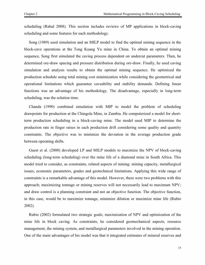
Song (1989) used simulation and an MILP model to find the optimal mining sequence in the
block-cave operations at the Tong Kuang Yu mine in China. To obtain an optimal mining
sequence, Song first simulated the caving process dependent on undercut parameters. Then, he
determined ore-draw spacing and pressure distribution during ore-draw. Finally, he used caving
simulation and analysis results to obtain the optimal mining sequence. He optimized the
production schedule using total mining cost minimization while considering the geometrical and
operational limitations which guarantee caveability and stability demands. Defining linear
functions was an advantage of his methodology. The disadvantage, especially in long-term
scheduling, was the solution time.
Chanda (1990) combined simulation with MIP to model the problem of scheduling
drawpoints for production at the Chingola Mine, in Zambia. He computerized a model for short-
term production scheduling in a block-caving mine. The model used MIP to determine the
production rate in finger raises in each production drift considering some quality and quantity
constraints. The objective was to minimize the deviation in the average production grade
between operating shifts.
Guest et al. (2000) developed LP and MILP models to maximize the NPV of block-caving
scheduling (long-term scheduling) over the mine life of a diamond mine in South Africa. This
model tried to consider, as constraints, related aspects of mining: mining capacity, metallurgical
issues, economic parameters, grades and geotechnical limitations. Applying this wide range of
constraints is a remarkable advantage of this model. However, there were two problems with this
approach; maximizing tonnage or mining reserves will not necessarily lead to maximum NPV;
and draw control is a planning constraint and not an objective function. The objective function,
in this case, would be to maximize tonnage, minimize dilution or maximize mine life (Rubio
2002).
Rubio (2002) formulated two strategic goals; maximization of NPV and optimization of the
mine life in block caving. As constraints, he considered geomechanical aspects, resource
management, the mining system, and metallurgical parameters involved in the mining operation.
One of the main advantages of his model was that it integrated estimates of mineral reserves and

Chapter 2 Mathematical Programming in Block-Caving Scheduling
16
the development rate that resulted from the production scheduling. Traditionally these
parameters were computed independent of production scheduling. Rubio also formulated a
relationship between the draw control factor and the angle of draw. This relationship was built
into the actual draw function to compute schedules with high performance in draw control.
Opportunity cost in block caving was defined as the financial cost of delaying production from
newer drawpoints; a drawpoint will stay active at any given period of the schedule, if it has
enough remaining value to pay the financial cost of delaying production from newer drawpoints
that may have a higher remaining value.
Rahal et al. (2003) described an MILP goal program with dual objectives of minimizing
deviation from the ideal draw profile while achieving a production target. They performed a
schedule optimization using a-life-of-mine approach in which all production periods were
optimized simultaneously. They assumed that material mixing in the short-term has a minimal
effectonthepanel’s long-termstate.Themodel’sconstraintsweredeviation from ideal practice,
panel state, material flow conservation, production quality, material flow capacity, and
production control. They applied the model to De Beers kimberlite mine. The results showed
how different production control constraints regulate production from individual drawpoints, as
well as recovery of the ideal panel profile by implementing an optimized draw schedule.
Diering (2004) described the basic problem in block-caving scheduling as trying to determine
the best tonnages to extract from a number of drawpoints for various periods of time. Those
periods could range from a day to the life of the mine. Diering singled out NPV as the overall
objective to maximize, subject to some constraints: minimum tonnage per period, maximum
tonnage per period, maximum total tonnage per drawpoint, maximum total tonnage per period,
ratio of tonnage from current drawpoint compared with neighbors, height of draw of current
drawpoint with respect to neighbors, percentage drawn for current drawpoint with respect to
neighbors, and maximum tonnage from selected groups of drawpoints in a period (usually the
groups of drawpoints are referred to as production blocks or panels). Diering emphasized that it
would be better to formulate the problem as an LP instead of NLP because of solution time and
the size of problems. He applied a multi-step non-linear optimization model to minimize the
deviation between a current draw profile and a defined target. It was shown that this algorithm
could also be used to link the short-term plan with the long-term plan.

Chapter 2 Mathematical Programming in Block-Caving Scheduling
17
Rubio and Diering (2004) applied MP to maximize the NPV, optimize the draw profile and
minimize the gap between long- and short-term planning. They integrated the opportunity cost
into GEOVIA PCBC for computing the best height of draw in a dynamic manner. To solve their
problem, they used different mathematical techniques such as direct iterative methods, LP, a
golden section search technique, and integer programming. In their formulation, mining reserves
were not part of the set of constraints; the mining reserves were computed as a result of the
optimal production schedule. They also used QP to minimize the differences between actual
heights of draw versus a desired target.
Rahal (2008) presented a draw control model that indirectly increases resource value by
controlling production based on geotechnical constraints. He used MILP to formulate a goal
programming model with two strategic targets: total monthly production tonnage and cave shape.
This approach increased value by ensuring that reserves are not lost due to poor draw practice.
Themodel’sadvantagewasthatitallowsanynumberofprocessingplantstofeedfrom multiple
sources (caves, stockpiles, and dumps). There were three main production control constraints in
the MILP: the draw maturity rules, minimum draw rate, and relative draw rate (RDR). Rahal
used MILP to quantify production changes caused by varying geotechnical constraints, limiting
haulage capacity, and reversing mining direction. He showed that tightening the RDR constraint
decreases total cave production. He applied his model for three case studies and illustrated how
the MILP can be used by a draw control engineer to analyze production data and develop long-
term production targets both before and after a cave is brought into full production.
Rahal et al. (2008) used MILP to develop an optimized production schedule for Northparkes
E48 mine. They described the system constraints as minimum and maximum draw tonnage, the
permissible relative draw rate difference between adjacent drawpoints, drawpoint availability,
and the capacity of the materials handling system. The impact of different production constraints
on total cave capacity was examined. It was shown that the strength of using MILP lies in its
ability to generate realistic production schedules that require little manual manipulation.
Weintraub et al. (2008) developed an approach to aggregate the reduced models (which have
been derived from a global model) using the original data for an MIP mine planning model in a
large block-caving mine. The aggregation was based on clustering analysis. The MIP model was
developed to support decisions for planning extraction of blocks and the decisions of exact
Chapter 2 Mathematical Programming in Block-Caving Scheduling
18
timing for each block in the extraction columns. The final model was developed to integrate all
mines for corporate decisions, to determine extraction from each sector, in each mine, for each
period (for a five-year horizon). Weintraub et al. used two types of aggregation: Priori
aggregation and Posteriori approach. Comparing the original model with the disaggregation, the
first approach reduced execution time by 74% and the model dimension by 90%. The second
approach reduced solution time by 88% and the model dimension by 15%.
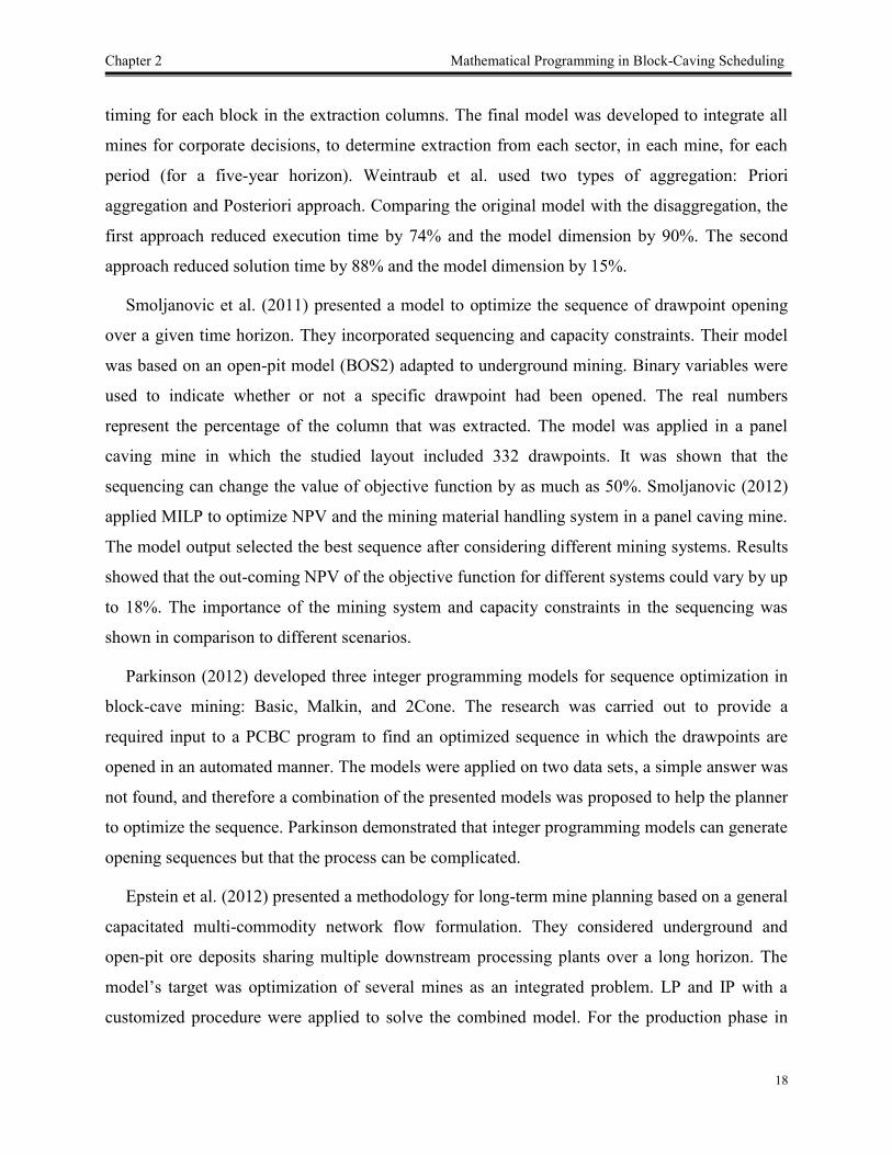
Smoljanovic et al. (2011) presented a model to optimize the sequence of drawpoint opening
over a given time horizon. They incorporated sequencing and capacity constraints. Their model
was based on an open-pit model (BOS2) adapted to underground mining. Binary variables were
used to indicate whether or not a specific drawpoint had been opened. The real numbers
represent the percentage of the column that was extracted. The model was applied in a panel
caving mine in which the studied layout included 332 drawpoints. It was shown that the
sequencing can change the value of objective function by as much as 50%. Smoljanovic (2012)
applied MILP to optimize NPV and the mining material handling system in a panel caving mine.
The model output selected the best sequence after considering different mining systems. Results
showed that the out-coming NPV of the objective function for different systems could vary by up
to 18%. The importance of the mining system and capacity constraints in the sequencing was
shown in comparison to different scenarios.
Parkinson (2012) developed three integer programming models for sequence optimization in
block-cave mining: Basic, Malkin, and 2Cone. The research was carried out to provide a
required input to a PCBC program to find an optimized sequence in which the drawpoints are
opened in an automated manner. The models were applied on two data sets, a simple answer was
not found, and therefore a combination of the presented models was proposed to help the planner
to optimize the sequence. Parkinson demonstrated that integer programming models can generate
opening sequences but that the process can be complicated.
Epstein et al. (2012) presented a methodology for long-term mine planning based on a general
capacitated multi-commodity network flow formulation. They considered underground and
open-pit ore deposits sharing multiple downstream processing plants over a long horizon. The
model’s targetwas optimization of severalmines as an integratedproblem.LP and IPwith a
customized procedure were applied to solve the combined model. For the production phase in

Chapter 2 Mathematical Programming in Block-Caving Scheduling
19
underground mine, which it was block caving, constraints were production per sector, product
and period, production cost, extraction times for each block (at most once), block and period
priority, minimum blocks for each column, order of drawpoints, maximum duration of a
drawpoint, extraction rate of each column, the column in each period, similarity of heights in
neighboring columns, bounds on the area, extracted rock per period, and each sector extraction
within its time window. The model developed by Epstein et al. has been implemented at
Codelco, production plans for a single mine and integrating multiple mines increased the NPV.
Diering (2012) used QP techniques for block-caving production scheduling, focusing on
single-period formulations. He explained that the block caving process is non-linear (the tons
which you mine in later periods will depend on the tons mined in earlier periods), so it would not
be appropriate to use LP for production scheduling in block caving. The objective function was
the shape of the cave. Three sets of constraints were applied in the model: mandatory, modifying,
and grade-related. This formulation omitted the sequence of drawpoint development (interaction
between neighboring drawpoints) as a constraint.
Pourrahimian et al. (2012) presented two MILP formulations at two different levels of
resolution: (i) drawpoint level, and (ii) aggregated drawpoints (cluster level). The objective
function was to maximize the NPV. They usedPCBC’sslicefileasaninputintotheirmodel,but
their models treat the problem in the drawpoint or cluster level as a strategic long-term plan, and
the slices are not used in the presented formulations. To reduce the number of binary variables,
Pourrahimian et al. used Fuzzy c-means clustering to aggregate the drawpoints into clusters
based on similarities between draw columns and the physical location of the drawpoint and its
tonnage. They used same data for both models and solved the problem for four different
advancement directions. The execution time for aggregated drawpoints was reduced by more
than 99%.
Pourrahimian et al. (2013) developed a theoretical optimization framework based on a MILP
model for block-cave long-term production scheduling. The objective function was to maximize
the NPV. They formulated three MILP models for three levels of problem resolution: cluster
level, drawpoint level, and drawpoint-and-slice level. They showed that the formulations can be
used in both the single-step method, in which each of the formulations is used independently;
and as a multi-step method, in which the solution of each step is used to reduce the number of

Chapter 2 Mathematical Programming in Block-Caving Scheduling
20
variables in the next level and consequently to generate a practical block-cave schedule in a
reasonable amount of CPU runtime for large-scale problems. They considered mining capacity,
grade blending, the maximum number of active clusters or drawpoints, the number of new
clusters or drawpoints, continuous mining, mining precedence, reserves, and the draw rate as
constraints which were involved in all three levels of resolutions. Using such a flexible
formulation is very helpful because depending on the level of studies — prefeasibility studies
(PFS), feasibility studies (FS) or detailed feasibility studies (DFS) — a mine planner can use the
appropriate level of solution and the related runtime. They developed and tested their
methodology in a prototype open-source software application with the graphical user interface
DSBC (Drawpoint Scheduling in Block-Caving).
Alonso-Ayuso et al. (2014) considered uncertainty in copper prices along with a given time
horizon (five years) using a multistage scenario tree to maximize the NPV of a block-cave mine
in Chile, then the stochastic model was converted into a MIP model. They applied the stochastic
model in both risk-neutral and risk-averse environments. Results showed the advantage of using
the risk-neutral strategy over the traditional deterministic approach, as well as the advantage of
using any risk-averse strategy over the risk-neutral one.
Rubio (2014) introduced the concept of portfolio optimization for block caving. In this
method, every decision related to mine design and mine planning could be a component of a set
that defines a feasible portfolio. This set is optimized for different production targets to
maximize the return subject to a given level of reliability. Using this approach, a frontier
efficient is proposed as a boundary to display different strategic designs and planning options for
the set of variables under study. By this method, decision makers can define a point along the
frontier efficient where they want to place a given project.
Khodayari and Pourrahimian (2014) proposed a model in which the best height of draw
(BHOD) is determined as part of the sequence optimization in block caving. In other words, the
mining reserve was an output of the optimization, not an input. In another paper, they presented a
methodology to find the best mining direction in the block caving layout (Khodayari and
Pourrahimian 2015a). Total dollar values of draw columns located in different neighborhoods
were used to determine the direction and then the precedence of extraction among drawpoints.
Khodayari and Pourrahimian (2016) also proposed a mixed integer quadratic programming
Chapter 2 Mathematical Programming in Block-Caving Scheduling
21
(MIQP) model for production scheduling, the goal was to achieve a uniform extraction profile in
order to reduce the potential dilutions in the production. They also presented an MILP model to
optimize the production schedule during the life of the mine while taking the material flow into
account (Khodayari and Pourrahimian 2017). Their stochastic optimization model was based on
a mixing environment that includes a set of draw columns that are located in the same
neighborhood. Using this methodology, the resulting schedule is more reliable as it is closer to
what happens in the real-world operations, it was recommended to develop the objective function
and the mixing approach.
Nezhadshahmohammad et al. (2017) proposed an MILP model to maximize the NPV with
consideration of draw rate curve as a geotechnical constraint. Nezhadshahmohammad et al.
(2017) used a clustering model to optimize a long-term production schedule for block caving
operations. They also used a draw control system within the neighborhood while maximizing the
NPV of the project. Malaki et al. (2017) applied sequential Gaussian simulation and MILP to
find the best level of extraction in block caving while considering the grade estimation
uncertainties.
Sepúlveda et al. (2018) used a multi-objective optimization approach to maximize the
economic return of block-cave mining operations while minimizing the risk associated with
geometallurgical uncertainty. It was shown that the combination of maximization of economic
values and minimization of deviations from production targets results in lower risks in an
uncertain environment. They recommended the incorporation of caving flow into the production
schedule for future research. Another stochastic optimization model was proposed by Dirkx et al.
(2018) to include the uncertainty of grade and resulting delays from hang-ups into the production
schedule. Testing the model for a low-grade copper deposit showed an improvement in the NPV
compared to deterministic models. Table 2.1 shows the summary of the aforementioned MP
applications in block-caving scheduling.
GEOVIA PCBC is the most used commercial software in block caving mines. The program is
integrated into a general purpose geological modeling and mine planning system so that it can be
used for studies ranging from pre-feasibility to daily draw control. The simulation of mixing is
an important part of the program. PCBC simulates the extraction from each active drawpoint

Chapter 2 Mathematical Programming in Block-Caving Scheduling
22
period-by-period subject to a range of constraints and inputs (Diering 2000). More details about
GEOVIA PCBC is presented in section 5.1 where it is used for validation of the BCSO.
Table 2.1. Summary of applied MP models in block-caving production scheduling
Author Model Model objective(s) Constraint(s)
Song (1989) Simulation
and MILP
Minimization of total mining
cost
Geometrical limitations
Operational limitations
Chanda (1990) Simulation
and MIP
Minimization of the deviation in
the average production grade
between operating shifts
Maximum allowable output per shift
Maximum allowable number of working
drawpoints per shift
Declaration of exhaustion for exhausted
drawpoints
Required grade for each shift (equality)
Tonnage of blended ore in each shift
Guest et al.
(2000) LP and MILP Maximization of NPV
Geotechnical constraints
Column draw rates
Precedence of accumulated tons drawn
Limits in differences of accumulated tons
drawn between columns within time
horizons
Limits in ratios of tons drawn between
columns (neighbors) within time horizons
Mining constraints
Ore flow constraints (tunnels, ore passes,
haulage, underground accumulation areas,
shaft systems)
Metallurgical constraints
Treatment plant (capacities per period)
Economic constraints (revenue, costs)
Geological constraints (grade, size)
Rubio (2002) MILP and
NLP
Two models (a) maximization of
NPV and (b) optimization of the
mine life
Development rate
Undercut sequence
Drawpoint status
Maximum opened production area
Draw rate
Period constraints
Mining reserves
Rubio and
Diering (2004) MILP and QP
Maximization of NPV,
optimization of draw profile, and
minimization of the gap between
long- and short-term planning
Development rate
Undercut sequence
Maximum opened production area
Draw rate
Draw ratio
Period constraints

Chapter 2 Mathematical Programming in Block-Caving Scheduling
23
Table 2.1. Summary of applied MP models in block-caving production scheduling (continued)
Author Model Model objective (s) Constraint(s)
Diering (2004) NLP
Maximizing NPV for M periods
and minimization of the
deviation between a current
draw profile and a defined target
Minimum and maximum tonnage per period
Maximum total tonnage per drawpoint and
per period
Ratio of tonnage from current drawpoint
compared with neighbors.
Height of draw of current drawpoint with
respect to neighbors
Percentage drawn for current drawpoint
with respect to neighbors
Maximum tonnage from selected groups of
drawpoints in a period
Rahal (2008) MILGP
Minimizing deviation from the
ideal draw profile while
achieving a production target
Deviation From Ideal Plan
Ideal depletion
Panel production rate
Production from external sources
Contents of material sources
Material flow conservation (blocks, tunnels,
ore pass, haulage, accumulation, shaft,
plant)
Material flow and capacity (source flow,
block, externals, ore pass, haulage,
accumulation, shaft, plant)
Production Control
Block available for draw
Relative draw rate
Block flow bounds
Draw maturity rules (Lower Depletion
Bound/Upper Production Bound)
Product quality and quantity
Economics
Weintraub et
al. (2008) MIP Maximization of profit
Each cluster can be extracted only once
Sequence of extractions
The allowable speed
Capacity of extraction
Conservation of flows and logical
relationships between variables
Smoljanovic
et al. (2011) MILP
Optimization of NPV and
mining material handling system
Production Constraints
Max and min amount of tonnage to be
extracted per time period
The overall mine capacity

Chapter 2 Mathematical Programming in Block-Caving Scheduling
24
Table 2.1. Summary of applied MP models in block-caving production scheduling (continued)
Author Model Model objective(s) Constraint(s)
Smoljanovic
et al. (2011)
(continued)
MILP Optimization of NPV and
mining material handling system
Total number of drawpoints to be opened at
each time period
Capacity per drawpoint
Min percent of extraction for each
drawpoint
Lifetime of a drawpoint
Capacity of haulage system
Geometric constraints
Connectivity and shape constraints
Epstein et al.
(2012) MIP Maximization of NPV
Production per sector (product and period)
Production cost
Extraction times for each block
Block and period priority
Minimum blocks for each column
Order of drawpoints
Maximum duration of a drawpoint
Extraction rate of each column
The column in each period
Neighboring columns heights similarity
Bounds on the area
Extracted rock per period
Each sector extraction within its time
window
Parkinson
(2012)
IP Finding an optimal opening
sequence in an automated
manner
Each drawpoint starts once
Global capacity (processing plant capacity)
Tunnel development
Additional constraints:
Within-tunnel contiguity
Across-tunnel contiguity
Diering (2012) QP
Objective tonnage
(to optimize the shape of the
cave)
Mandatory constraints
Production capacity
A maximum tonnage for each drawpoint
based on the drawpoint maturity curve
A minimum tonnage for each drawpoint.
Modifying constraints
Maximum tonnage from production tunnels
Maximum tonnage from an orepass or
crusher
Maximum tonnage from an entire sector
Grade-related constraints

Chapter 2 Mathematical Programming in Block-Caving Scheduling
25
Table 2.1. Summary of applied MP models in block-caving production scheduling (continued)
Author Model Model objective(s) Constraint
Pourrahimian et
al. (2013) MILP Maximization of NPV
Mining capacity
Grade blending
Maximum number of active clusters or
drawpoints (according to the model
resolution)
Number of new clusters or drawpoints
(according to the model resolution)
Continuous mining
Mining precedence
Slice
Drawpoint
Cluster
Reserves
Draw rate
Draw column
Cluster
Alonso-Ayuso et
al. (2014) MILP
Maximization of NPV while
considering uncertainty in
copper price
Each cluster is processed at most once
If a cluster is processed at a given period
then all predecessor clusters are also
processed by that period
The clusters in each set would be extracted
simultaneously in each sector
Number of tons processed in each sector at
each period
Flow conservation constraints for the
processing stream
Number of tons processed in each period
Upper and lower bounds for the total area
processed in each sector
Number of tons processed in each period
Upper bound due to the capacity of
processing stream
The maximum increase and decrease of tons
in each sector in each period
Khodayari and
Pourrahimian
(2014)
MILP Maximization of NPV and
finding the BHOD
Mining capacity
Production grade
Number of active drawpoints
Continuous mining
Mining precedence
Reserves
Draw rate
Khodayari and
Pourrahimian
(2015a)
LP Finding the best mining
direction -

Chapter 2 Mathematical Programming in Block-Caving Scheduling
26
Table 2.1. Summary of applied MP models in block-caving production scheduling (continued)
Author Model Model objective(s) Constraint
Khodayari and
Pourrahimian
(2016)
MIQP Achieving smoother caving
shape to reduce the dilution
Mining capacity
Production grade
Number of active drawpoints
Continuous mining
Mining precedence
Reserves
Khodayari and
Pourrahimian
(2017)
MILP
(Stochastic)
Maximization of NPV and
incorporation of material flow
in the optimization model
Mining capacity
Production grade
Number of active drawpoints
Continuous mining
Drawpoint precedence
Slice precedence
Reserves
Draw rate
Draw life
Grade deviations
Nezhadshahmoha
mmad et al.
(2017)
MILP Maximization of NPV
Mining capacity
Production grade
Number of active drawpoints
Continuous mining
Mining precedence
Reserves
Draw rate
Number of new drawpoints
Nezhadshahmoha
mmad et al.
(2017)
MILP Maximization of NPV
Mining capacity
Production grade
Number of active drawpoints
Continuous mining
Mining precedence
Reserves
Draw rate
Draw life
Number of new drawpoints
Malaki et al.
(2017) MILP
Finding the best level of
extraction while considering the
grade estimation uncertainties
Mining capacity
Production grade
Continuous mining
Mining precedence
Reserves
Number of new big blocks

Chapter 2 Mathematical Programming in Block-Caving Scheduling
27
Table 2.1. Summary of applied MP models in block-caving production scheduling (continued)
Author Model Model objective(s) Constraint
Sepúlveda et al.
(2018)
MILP
(Stochastic)
Maximization of the net smelter
return and reducing
geometallurgical uncertainty
Mining capacity
Grade blending
Maximum number of active drawpoints
Continuous mining
Mining precedence
Reserves
Draw rate
Draw life
Number of new draw-points
Dirkx et al.
(2018)
MILP
(Stochastic)
Maximization of NPV and
minimizing deviations from
targets
Extraction capacity
Drawpoint precedence
Slice precedence
Continuous mining
Ratio of extraction between adjacent
drawpoints
Deviations of hang-up delays
Tonnage deviations
Grade deviations
Bottleneck constraints
Reserve
In mathematical programming, we look for values of variables which are allowed and do not
violate the constraints. This defines what is called a solution space, in which the edges of this
space are the constraints. In case of an LP formulation, the solution must be on a boundary of
this space. In the case of block-cave scheduling, an LP formulation will always seek to take the
maximum tons from the highest value drawpoints and the least tons from the lower valued
drawpoints (Diering 2012). As a result, this kind of scheduling may result in high levels of
horizontal mixing between drawpoints because the draw columns have different heights. This is
a potential disadvantage of LP application in block-caving scheduling. Table 2.2 summarizes the
advantages and disadvantages of methodologies examined in previous studies.

Chapter 2 Mathematical Programming in Block-Caving Scheduling
28
Table 2.2. Advantages and disadvantages of applied mathematical methodologies in block-caving production
scheduling
Methodology Features
LP
Advantage LP method has been used most extensively (Rahal 2008)
It can provide a mathematically provable optimum schedule (Rahal, 2008)
Disadvantage
Straight LP lacks the flexibility to directly model complex underground
operations which require integer decision variables (Winkler 1996)
Mine scheduling is too complex to model using LP and the only possible
approach is to use some combination of theoretical and heuristic methods to
ensure a good, if not optimal schedule (Scheck et al. 1988)
MILP
Advantage
Computational ease in solving a MIP problem (and MILP) is dependent upon the
formulation structure (Williams 1974)
MILP could be used to provide a series of schedules which are marginally inferior
to a provable optimum (Hajdasinski 2001)
MILP is superior to simulation when used to generate sub-optimal schedules,
because the gap between the MILP feasible solution and the relaxed LP solution
provides a measure of solution quality (Rahal 2008)
MILP can provide a mathematically provable optimum schedule (Rahal 2008)
Disadvantage
It is often difficult to optimize large production systems using the branch-and-
bound search method (Rahal 2008)
The block-caving process is non-linear (the tons which you mine in later periods
will depend on the tons mined in earlier periods), so it would not be appropriate to
use LP for production scheduling in block caving (Diering 2012)
QP (MIQP)
Advantage
Since the block-caving process is non-linear, QP could be an appropriate option to
model it
It can find solutions in the interior of the solution space, which results in an even
height of drawpoints as well as lower horizontal mixing between drawpoints
(Diering 2012)
Disadvantage Solving this kind of problem could be a challenge. It must be changed to LP and
then be solved, to ensure conversion errors
Stochastic
Optimization Advantages
It can capture the uncertainties of the caving operations such as: material flow,
hang-ups, production grades, and production tonnages
Disadvantage The solution time is usually more than deterministic models
2.2. Material Flow
The literature on material flow can be divided into three categories: numerical models, pilot
tests, and full-scale experiments. As part of the development of FlowSim software, Castro R et
al. (2009) used numerical methods to simulate the gravity flow of caved rock. They calibrated
the proposed model with real data from two mining operations in Chile. Another numerical
model was developed by Pierce (2010), he used discrete element method to identify different
zones of movement (or isolations) in the caved material.

Chapter 2 Mathematical Programming in Block-Caving Scheduling
29
A stochastic approach was proposed by Gibson (2014) to study the material flow in block-
cave operations. He used Pascal cone theory to assess the probabilities of material that move
within their neighborhood when an empty space is created because of extraction from
drawpoints. He found it useful to use stochastic models instead of Finite Element methods
although it needs a certain amount of information about the rock mass. The cell size was one of
themaincriteriaintheGibosn’smodel, and any changes can remarkably affect the results.
Castro RL et al. (2014) designed a test setup to study the flow mechanisms of cohesionless
material when extracting from a single drawpoint. It was shown that the fragmentation size, the
diameter of the opening, and the vertical load (the amount of material above a drawpoint) are the
factors that affect the material flow. Jin et al. (2017) studied the shape of the ellipsoid draw by
some pilot tests; they proposed a new methodology to predict the extraction and movement zone
shapes and their change trends. Brunton et al. (2016) performed a full-scale experiment in
Ridgeway Deeps and Cadia East block caving mines in Australia. They used markers to quantify
and assess the development and shape of the extraction zone and find the mechanisms that
control the flow behavior. It was shown that marker experiments can provide a good
understanding about development of the extraction zone during undercutting and production
stages.
Garcés et al. (2016) applied smart marker technology in block 2 of Esmeralda mine, El
Teniente to study the gravity flow. The main objectives were to check the interaction between
extraction zones, estimate the mining recovery, evaluate the flow characteristics of caved rock,
and develop a model for flow. Results showed that the extraction zone mainly depends on the
fragmentation condition and the mine plan which means these two are interconnected. It was also
observed that the horizontal mixing is higher in the case of a non-concurrent draw. Using particle
flow code (PFC), Sun et al. (2018) developed a material flow simulation model that takes into
account the effects of particle bond strength on the secondary fragmentation and isolated zones
in the caving. They tested the model against experimental results; it was shown that the isolated
zones are wider in the case of weaker rock when the secondary fragmentation results in smaller
average fragment size and more fines.

Chapter 2 Mathematical Programming in Block-Caving Scheduling
30
2.3. Summary
Increasing the use of block caving in new-world mining environments has led many
researchers to focus on this area to make mining operations as optimal as possible. Production
scheduling in block caving, becauseof its significant impact on the project’s profitability and
feasibility, has been considered a key issue to be improved. The problem is complex, unique for
each case, and large-scale. Researchers have applied different methods to model production
scheduling in block caving, for short-term and long-term periods of mining, some for real case
studies as industry projects and others as academic research projects.
Most of the researchers have applied MILP to model production scheduling; it can be useful
because both the integer variables (whether a block, slice, or draw column should be extracted)
and continues variables (the constraints and mining operation details) can be modeled so that the
optimal values can be achieved while considering the system’sconstraints.
As computer based algorithms are improved, we expect to see the development of more
detailed models with more complexity, models that try to be more practical and include all
aspects of mining systems with new algorithms for faster solutions. In block-caving operations,
decisions about current actions are often based on how those actions affect the next steps in the
operations.
There are some uncertainties in block-cave mining that should be involved in production
scheduling. Grade uncertainty is one of the most common, because of the nature of ore-body, but
in block-caving operations grade uncertainty is more critical and complicated, due to the vertical
and horizontal mixing which occurs during the caving and production. Once the rock is
fragmented, particles flow towards the production level in different ways depending on the
fragmentation profile and distribution.
In summary, a significant amount of research exists in production scheduling optimization
and material flow; however, both concepts have been investigated separately, and there is a gap
of optimizing the mine plan with the material flow consideration. An optimized mine plan will
provide a guide towards a successful operation, and a material flow simulation model can give us
a valuable understanding of the caving process; however, these two will not be helpful enough if
they are not studied simultaneously. The goal of this research is to take into consideration the
material flow uncertainties as part of the production scheduling optimization; in other words, to

Chapter 2 Mathematical Programming in Block-Caving Scheduling
31
have an optimum production schedule in which not only the technical constraints are satisfied
but also the material mixing is incorporated into the optimization. This approach results in
achieving more reliable mine plans for block caving mines.

32
Chapter 3 Optimization of Production Scheduling in Block Caving
Operations with Consideration of Grade Targets
Chapter 3 describes an optimization model that maximizes the NPV of caving operations
while minimizing deviations from grade targets. In this model, the mixing occurs within draw
columns on a big scale. First, the methodology is presented and then the model is tested on a
real block caving mine. A version of this chapter has been published in Aspects of Mining and
Mineral Science, in 2017.
Khodayari F, Pourrahimian Y. 2017. Production scheduling in block caving with consideration
of material flow. Aspects in Mining and Mineral Science (AMMS). 1(1).

Chapter 3 Production Scheduling with Consideration of Material Flow
33
3.1. Introduction
Any planning and financial analysis in a mining project depends on the production schedule
in which the amount of ore and waste removal in each period of time is determined. An optimum
reliable production schedule can significantly improve the overall practicality and profitability of
the project. Block-cave mining operation is involved with uncertainties that should not be
ignored in the production scheduling; while the caving is occurring, the flow of material (which
happens because of the gravity) can be unpredictable. This will result in grade and tonnage
uncertainties in the production during the life of the mine. Numerical methods are useful tools to
model the material flow and using stochastic optimization, it is possible to capture the
uncertainty of material flow while optimizing the production schedule.
Production schedule in a block-cave mine can be investigated from different levels of
resolutions: cluster level, drawpoint level, or slice level (Pourrahimian et al. 2013). In this
research, the slices are the decision units. The output of the production schedule at this level
would be the periods in which each of the slices within a draw column is extracted and sent to
the processing plant. These decisions are made based on the defined goal(s) in the objective
function while considering the limitations of the operations as the constraints of the model. The
proposed production scheduling model is a stochastic optimization model in which the net
present value of the project is maximized during the life of the mine while the deviations from
target production grade(s) are minimized. Different scenarios of grade for the slice model are
generated to capture the uncertainty of the production grade that exists in the material flow
during production.
3.2. Methodology
The proposed model maximizes the NPV of the mining project during the life of mine while
minimizing the deviations of production grade from target grade(s). To be able to capture the
uncertainty of production in block-cave mining, the model is a stochastic optimization in which
different scenarios of grade mixing are considered. The formulation of the objective function was
inspired by a stochastic optimization model which was used by MacNeil and Dimitrakopoulos
(2017) for determining the optimal depth of transition from open-pit to underground mining. The
scenarios are defined based on the grade distribution in the mineral reserve. Each scenario
represents one circumstance that can happen during the production based on the flow of the

Chapter 3 Production Scheduling with Consideration of Material Flow
34
material. Figure 3.1 shows the flow of material between draw columns and how it can impact the
production.
Figure 3.1. Material flow and its impact on the production grade
While extracting from a drawpoint (DP8), material can move not only from the column above
(DC8) but also from the columns located in its neighborhood (DC1…DC7) into the intended
drawpoint (DP8). This material movement during the caving is the main source of the
uncertainties in the operations. A production schedule would be more reliable if these
uncertainties are captured. As it was mentioned, the decision units for the proposed model in this
paper are the slices; the slice model is built based on the resource block model, the column above
each drawpoint is divided into slices. In this section, the mathematical programming model is
presented in details.
3.2.1. Notation
Indices
{1,..., }t T Index for scheduling periods.
{1,..., }sl Sl Index for individual slices.

Chapter 3 Production Scheduling with Consideration of Material Flow
35
{1,..., }dp Dp Index for individual drawpoints.
{1,..., }s S Index for individual scenarios.
{1,..., }a A Index for the adjacent drawpoints.
{1,..., }j J Index for individual production blocks.
Variables
t
slX Binary decision variable that determines if slice " "sl is extracted in
period " "t ( 1t
slX ) or not ( 0t
slX ).
t
dpY Binary decision variable which determines whether drawpoint " "dp in
period " "t is active ( 1t
dpY ) or not ( 0t
dpY ).
t
dpZ Binary decision variable which determines whether drawpoint dp at
period " "t (periods 1, 2,..,t) has started its extraction ( 1t
dpZ ) or not (
0t
dpZ ).
[0, ] t
usd Continuous decision variable representing excessive amount from the
target grade (the metal content).
[0, ] t
lsd Continuous decision variable representing deficient amount from the
target grade (the metal content).
Model Parameters
slg Copper (Cu) grade of slice " "sl .
Eslg Expected (average) copper grade for slice " "sl based on all scenarios.
slton Ore tonnage of slice " "sl .
ct Current period.
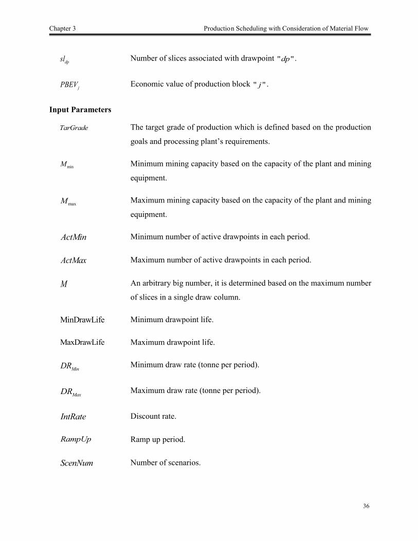
Chapter 3 Production Scheduling with Consideration of Material Flow
36
dpsl Number of slices associated with drawpoint " "dp .
jPBEV Economic value of production block " "j .
Input Parameters
TarGrade The target grade of production which is defined based on the production
goalsandprocessingplant’srequirements.
minM Minimum mining capacity based on the capacity of the plant and mining
equipment.
maxM Maximum mining capacity based on the capacity of the plant and mining
equipment.
ActMin Minimum number of active drawpoints in each period.
ActMax Maximum number of active drawpoints in each period.
M An arbitrary big number, it is determined based on the maximum number
of slices in a single draw column.
MinDrawLife Minimum drawpoint life.
MaxDrawLife Maximum drawpoint life.
MinDR Minimum draw rate (tonne per period).
MaxDR Maximum draw rate (tonne per period).
IntRate Discount rate.
RampUp Ramp up period.
ScenNum Number of scenarios.

Chapter 3 Production Scheduling with Consideration of Material Flow
37
ct
dpDP Drawpoint depletion percentage which is the portion of draw column dp
which has been extracted from drawpoint " "dp till period " "ct .
Price Copper price ($/tonne).
Cost Operating costs ($/tonne).
uC Cost (penalty) for excessive amount ($).
lC Cost (penalty) for deficient amount ($).
Rec Recovery of the processing plant (%)
3.2.2. Objective Function
The objective function is defined as follows:
1 1 1 1
{( )} { }
T Sl T S
t t t
sl sl s
t sl t s
Maximize E NPV X Grade deviations
1 1
1 1
( ( /100)) ( os )
(1 )
1( )
(1 )
T SltEsl sl slslt
t sl
t tT Sls l us u
tt s
Price Rec g ton C t tonX
IntRate
d c d c
S IntRate
(3.1)
The first part of the objective function maximizes the NPV of the project during the life of the
mine by finding the optimum sequence of extraction for the slices in the mineral reserve. The
second part minimizes deviations of the production grades from the targets in different scenarios
during the life of the mine, this is done by allocating penalties to the deviations in different
scenarios.
3.2.3. Constraints
Operational and technical constraints of block-cave mining are considered to control the
practicality of the production schedule. Total number of decision variables depends on the
number of drawpoints, the number of slices in each drawpoint, and the production timeline.

Chapter 3 Production Scheduling with Consideration of Material Flow
38
Logical constraints
There are two extra sets of binary decision variables in the proposed model which will be
required for defining different constraints (" , "Y Z ). Logical constraints connect the main
decision variables (" "X ) to the new decision variables (" , "Y Z ), each set contains two
inequality equations:
[0,1],
t
dp
dp DpY
t T
1
{1,..., } {1,..., } 0&
dpsl
t t
dp sl
sl
t T dp Dp Y M X (3.2)
1
{1,..., } {1,..., } * 0&
dpsl
t t
sl dp
sl
t T dp Dp X M Y (3.3)
[0,1],
t
dp
dp DpZ
t T
1
{1,..., }
c
c
tt t
dp dp
t
dp Dp DP Y (3.4)
{1,..., } {1,..., } * 0& ct t
dp dpt T dp Dp DP M Z (3.5)
{1,..., } {1,..., } * 0& ctt
dp dpt T dp Dp Z M DP (3.6)
Mining Capacity
Mining capacity is limited based on the production goals and availability of equipment.
maxmin1
{1,..., }
Sl
tsl sl
sl
t T M ton X M (3.7)
Production grade
This constraint ensures that the production grade is as close as possible to the target grade in
different scenarios.

Chapter 3 Production Scheduling with Consideration of Material Flow
39
Deviations from the target grade for all scenarios in different periods of production during the
life of the mine are considered for this constraint.
1
{1,..., } {1,..., } ) 0& (
l u
Slt
tarsl sl slsl
t T S d ds g G ton X (3.8)
Reserve
This constraint makes sure that not more than the existing mineral resources can be extracted,
the output of the model would be the mineral reserve.
1
{1,..., } 1
T
tsl
t
sl Sl X (3.9)
Active drawpoints
A limited number of drawpoints can be in operation at each period of time; the mining layout,
equipment availability, and geotechnical parameters can determine this constraint.
1
{1,..., }
Dp
t
dp
dp
t T ActMin Y ActMax (3.10)
Mining precedence (horizontal)
The precedence is defined based on the mining direction in the layout. Production from each
drawpoint can be started only if the drawpoints in its neighborhood which are located ahead
(based on the mining direction) have already been opened. Equation (3.12) presents this
constraint.
1
{1,..., } {1,..., } *&
A
t t
dp a
a
t T dp Dp A Z Z (3.11)
Where " "A is the number of drawpoints in the neighborhood of drawpoint " "dp which are
located ahead (based on the defined advancement direction) and " "Z is the second set of binary
variables. Advancement direction is the direction of mining among drawpoints in which, the
horizontal precedence among drawpoints is defined based on.
Mining precedence (vertical)

Chapter 3 Production Scheduling with Consideration of Material Flow
40
The precedence of extraction between slices within draw columns during the life of mine is
defined by this constraint.
1
1
{1,..., } {1,..., } {1,..., }& &
ct
t t
sl sl
t
t T dp Dp sl Sl X X (3.12)
This equation ensures that in each period of " "t , slice " "sl (in the draw column associated
with drawpoint " "dp ) is extracted only if slice " 1"sl located beneath is already extracted in
the periods before or at the same period (" "ct ).
Continuous mining
This constraint guarantees a continuous production for each of drawpoints during the life of
the mine. In other words, if a drawpoint is opened, it is active in consecutive years (with at least
the minimum draw rate of " "MinDR ) untill it is closed.
1{1,..., } {1,..., } (1 )& t t t
dp dp dpt T dp Dp Y Y Z (3.13)
Draw rate
The total production of each drawpoint in each period is limited to a minimum and maximum
amount of draw rate.
1
{1,..., } {1,..., }&
dpsl
t t
Min dp sl sl Max
sl
t T dp Dp DR Y ton X DR (3.14)
Draw life
Drawpoints can be in production during a certain time which is called draw life. The draw life
is limited to the minimum and maximum years of operations by the following equation:
1
{1,..., }
T
t
dp
t
dp Dp MinDrawLife Y MaxDrawLife (3.15)
3.2.4. Mining direction (mining advancement) determination
A more detailed version of this section was presented in the 5th International Symposium of
Mineral Resources and Mine Development by the authorof this research (Khodayari and
Pourrahimian 2015a).

Chapter 3 Production Scheduling with Consideration of Material Flow
41
In block-cave mining, production starts from one part of the ore-body and then inadirection
continues to the other side (s) of mining layout. For example, Figure 3.2 shows a mining
direction in which the drawpoints are opened from the north-east side of the layout and then the
extraction continues towards south-west (from A to B). Mining direction is determined based
on different factors such as geotechnical parameters of the ore-body and overburden, grade
distribution in different parts of the ore-body, commodity price, and equipment availability.
Figure 3.2. Example of mining direction for a block caving layout
The direction can be defined as a straight line (s), curve (s), or triangles. Based on the
proposed methodology in this research, at the first step, adjacent drawpoints are defined using
the distance between drawpoints so that combination of each drawpoint with its adjacent
drawpoints is called a production block (PB). Based on the locations of drawpoints in the
production layout, each drawpoint can appear in several production blocks with its different sets
of adjacent drawpoints. Therefore, in a layout with “n” drawpoints, there are “n” production
blocks. Figure 3.3 shows the schematic view of this methodology. In this figure, for the
considered drawpoint (the circle in the centre of the hatched block), the adjacent drawpoints are
determined using the defined adjacent radius of “R”. Depending on the geometry of the
production layout, there might be some production blocks with smaller number of drawpoints

Chapter 3 Production Scheduling with Consideration of Material Flow
42
compared to the other production blocks (this situation happens in the boundaries of the layout).
The adjacent radius is imported to the model as an input parameter and then the adjacent
drawpoints for each drawpoint is determined. The adjacent radius depends on different factors,
such as geotechnical parameters of the ore-body and its host rock (s), mining equipment, and
operational constraints.
Figure 3.3. Adjacent drawpoints for the considered drawpoint with the adjacent radius of R (small circles
represent the drawpoints)
In the input model, the draw economic value (DEV) for each draw column is calculated based
on the ore tonnages and grades of the slices. Using draw economic values, the summation of
DEV for each production block is calculated, and then the production block economic value
(PBEV) profile is created.
1 1 1
(Price Rec /100) ( )
A A Sl
j a sl sl sl
a a sl
PBEV DEV ton g Cost ton (3.16)
The adjacent drawpoints for each drawpoint are determined based on X and Y coordinates of
the drawpoints and then the production block economic values are calculated. In the next step,
the production block with the highest economic value is selected as the starting area. The
production is started from the neighbourhood with the maximum economic value and then it
continues to the areas with lower economic values. During the production periods, the economic

Chapter 3 Production Scheduling with Consideration of Material Flow
43
value of the current production block is equal or less than the previous one and greater or equal
than the next one.
For verification purposes, the methodology has been applied for a real case block-cave mining
project with 941 drawpoints (Figure 3.2). In total, 941 production blocks are defined for the
production layout based on the 25 meter adjacent radius. The results show that the central area of
the production layout is the best choice for starting the caving operation. Based on the
proposed methodology, two major directions are suggested for moving from the central part of
the ore-body to the boundaries. The mining directions are from the center to the east (direction 1)
and to the south (direction 2) of the layout (Figure 3.4).
Figure 3.4. Mining direction determination based on the PBEV concept
This methodology has been used to determine the mining direction and the horizontal
precedence in the other models presented in this research.

Chapter 3 Production Scheduling with Consideration of Material Flow
44
3.3. Solving the Optimization Problem
The proposed stochastic model has been developed in MATLAB (TheMathWorksInc. 2017),
and is solved in the CPLEX environment (IBM 2017). CPLEX uses branch-and-cut search for
solving the problem to achieve a solution within the defined mip gap (or the closest lower gap).
3.4. Case Study
The proposed model was tested on a block-cave mining operation with 102 drawpoints. It was
a copper-gold deposit with the total ore of 22.5 million tonnes and the weighted average grade of
0.85% copper. The draw column heights vary from 320 to 351 meters. Figure 3.5 and Figure 3.6
show the drawpoints layout (2D) and a conceptual view of the draw columns (3D). Each draw
column consists of a number of slices with the height of 10 meters (33 to 36 slices for each draw
column). In total, the model was built based on 3,470 slices. The goal is to produce a maximum
of 2 million tonnes of ore per year during 10 years of operations. The details of the input
parameters for the case study are presented in Table 3.1.
Figure 3.5. Drawpoint layout (circles represent
drawpoints)
Figure 3.6. A conceptual view of the draw columns
In this case study, different scenarios were created by generating random numbers in
MATLAB; a linear function was defined based on the original grades of the slices to produce
different scenarios. Also, the problem was solved as a deterministic model in which there were
no penalties for deviation from defined target grades, which means that the second part of the

Chapter 3 Production Scheduling with Consideration of Material Flow
45
objective function was not used. Production grades in different scenarios of the stochastic model
and the production grade resulting from the deterministic model are shown in Figure 3.7.
Table 3.1. Scheduling parameters for the case study
Parameter Value Unit Description
T 10 Year Number of periods (life of the mine)
Gmin 0.5 % Minimum average grade for Cu per each period
Gmax 1.6 % Maximum average grade for Cu per each period
GTar 1.3 % Target production grade (Cu)
Mmin 0 Mt Minimum mining capacity per period
Mst 0.5 Mt Mining capacity in the first year of production
Mmax 2 Mt Maximum mining capacity per period
Ramp-up 3 Year The time in which the production is increased from starting amount to the
full capacity
ActMin 0 - Minimum number of active drawpoints per period
ActMax 70 - Maximum number of active drawpoints per period
MIPgap 5 % Relative tolerance on the gap between the best integer objective and the
objective of the best node remaining
Radius 8.2 m The radius of the drawpoints
Density 2.7 t/m3 The average density of the material
M 100 - Arbitrary big number
MinDrawLife 0 Year Minimum life of drawpoints
MaxDrawLife 4 Year Maximum life of drawpoints
DRMin 13,000 Tonne/year Minimum draw rate
DRMax 75,000 Tonne/year Maximum draw rate
Recovery 85 % Recovery of the processing plant
Price 5,000 $/tonne Copper price per tonne of copper
Cost 15 $/tonne Operating costs per tonne of ore (Mining+Processing)
IntRate 10 % Discount rate
S 50 - Number of scenarios
It can be seen that for the stochastic model, production grades for all scenarios are as close as
possible to the defined target grade during the life of the mine. The deterministic model

Chapter 3 Production Scheduling with Consideration of Material Flow
46
maximizes the NPV and as a result the higher-grade ore is extracted earlier and then the lower
grades later during the life of the mine. The mining capacity constraint regulates ore production
and the ramp-up and ramp-down are almost achieved in both stochastic and deterministic models
(Figure 3.8 and Figure 3.9).
Figure 3.7. Average production grade resulting from stochastic and deterministic models
Figure 3.8. Ore production during the life of the mine (stochastic model)
Horizontal precedence, which is the precedence of extraction between drawpoints, was
achieved for both of models based on the defined V-shaped mining direction (Figure 3.10 and
Figure 3.11). Vertical precedence determines the precedence of extraction between slices in each
of draw columns.

Chapter 3 Production Scheduling with Consideration of Material Flow
47
Figure 3.9. Ore production during the life of the mine (deterministic model)
Figure 3.12 shows the resulted sequence of extraction among slices in draw column with ID
number of 75. Extraction from this drawpoint starts from year 5 and ends at year 8; the sequence
of extraction is from bottom to top and the production is continuous which means both the
vertical precedence and continuous mining constraints are satisfied.
Figure 3.10. Sequence of extraction for drawpoints resulting from the stochastic model (2D precedence)
The original height of draw column number 75 is 330.1 meters with the total ore of 212,397
tonnes which contains 34 slices. Based on the optimization results (Figure 3.12), the optimum

Chapter 3 Production Scheduling with Consideration of Material Flow
48
height of draw or BHD (Best Height of Draw) is 260 meters with the optimum draw tonnage of
168,650; this means that 26 out of 34 slices are extracted during the life of mine.
Figure 3.11. Sequence of extraction for drawpoints resulting from the deterministic model (2D precedence)
Number of active drawpoints and number of new drawpoints that are opened in each year for
both models are presented in Figure 3.13 and Figure 3.14. Comparing the new drawpoints to be
opened in each year for two models, the stochastic model does not suggest big changes from one
year to another while the deterministic model shows such a pattern. In other words, the results of
the stochastic model are more practical than the deterministic model.
Figure 3.12. Sequence of extraction for slices in draw column associated with drawpoint 75 (numbers represent ID
of slices in the draw column)

Chapter 3 Production Scheduling with Consideration of Material Flow
49
A brief comparison among the original ore resource model, the results of the deterministic
model, and the results of the stochastic model is presented in Table 3.2. For this case study, the
mining reserve and the NPV of the project for both models are almost the same (2% difference in
ore reserve and 0.7% difference in NPV). The stochastic model takes longer to solve, mainly
because of the required number of decision variables and constraints for each model.
Figure 3.13. Active and new opened drawpoints for the stochastic model
Figure 3.14. Active and new opened drawpoints for the deterministic model

Chapter 3 Production Scheduling with Consideration of Material Flow
50
Table 3.2. Comparing the original model with the results of deterministic and stochastic models
Comparison item
Original Model
(Mineral
resource)
Mineral reserve
Deterministic
Model Stochastic Model
Ore tonnage (Mt) 22.5 14 13.7
Number of slices 3,470 2,160 2,106
Average weighted grade (%) 0.85 1.28 1.3
Height of draw in individual draw columns 320-351 30-320 30-310
Number of slices in individual draw columns 33-36 3-32 3-31
NPV (M$) - 357.1 359.7
Solution time (Seconds) - 5,292 55,601
3.5. Summary
Production scheduling for block-cave mining operations could be challenging because of the
material flow uncertainties. In this chapter, a stochastic optimization model was proposed to
maximize the NPV of the project while minimizing the production grade deviations from the
target grades. Results show that stochastic models can be effective in production scheduling for
block-cave mining: the production goals are achieved, the constraints of the mining project are
satisfied, the uncertainty of the material flow is captured, the optimum height of draw (best
height of draw) is calculated as part of the optimization, and the net present value of the project
is maximized. Unlike deterministic models that do not consider the uncertainty of the material
flow, stochastic models can maximize the profitability of the project while taking mixing into
account for production scheduling. In the next chapters, consideration of both grade and tonnage
uncertainties in the production schedule as well as developing the methodology of generating
scenarios are discussed.

51
Chapter 4 Production Scheduling with Horizontal Mixing
Consideration in Block-cave Mining
Chapter 4 presents an optimization model to maximize the NPV and minimize deviations of
production grades and tonnages from the targets. Horizontal mixing is considered within slices
that are located in the same neighborhood. The model is introduced and implemented on a real-
case caving operation, and then the results are discussed.
A version of this chapter has been submitted to Journal of Mining Science and it is under review:
Khodayari F, Pourrahimian Y., Liu V. 2018. Production scheduling with horizontal mixing simulation in
block-cave mining. Journal of Mining Science, © Springer, (under review, 20 pages, June 2018).

Chapter 4 Production Scheduling with Horizontal Mixing
52
4.1. Introduction
Gravity is the main driver in block-cave mining: an undercut is developed beneath the
orebody, the rock fractures because of the created empty space, the caved material is extracted
using the designed drawpoints, and finally, the ore is transported to the surface for processing.
For scheduling purposes, the resulting block model from the resource estimation is used to create
a slice model where each slice is an aggregation of several blocks (Figure 4.1). Similar to blocks
in block model, each slice is represented by its grade, density, volume, and a decision variable
(for the mathematical modeling) in the slice model. Production scheduling for this type of
operation determines the mining direction in the layout as well as the amount of material to
extract from each drawpoint in each period.
Figure 4.1. Slice model
Similar to open-pit mining, production scheduling has significant impacts on the feasibility of
a mining project as it directly controls the cash flow. However, in block caving, because of the
uncertainties involved in the flow of the caved material, material movement influences the
production. As a result, the production scheduling optimization is more complicated, and an
optimum mine plan without consideration of the material flow can be impractical.
In this chapter, a stochastic optimization model is presented that aims to take some of the
uncertainties involved in material flow into production scheduling. To do this, the Height of
Interaction Zone (HIZ) is used to study theparticles’movements in theflow(Figure 4.2). The
slices that are located within the HIZ are directly extracted from their associated drawpoint
which means no horizontal mixing occurs.

Chapter 4 Production Scheduling with Horizontal Mixing
53
Figure 4.2. Horizontal mixing and its impact on production: below HIZ (left figure) and above HIZ (right figure)
Different scenarios are generated to simulate the potential horizontal movements of the
material within an adjacency radius from each slice. The aim is to achieve production targets and
maximize the net present value (NPV) of the mining project as well as consider the horizontal
mixing between draw columns as the caved rock is extracted from drawpoints. Integer and
continuous decision variables in the stochastic mixed-integer optimization model represent
slices, drawpoints, and deviations from targets. In addition, the best height of draw (BHOD) is
calculated as part of the optimization, which means that this part of optimization is also included
in the production scheduling.
4.2. Problem Statement and Formulation
In this section, formulations of the proposed model are presented. The model includes
technical constraints that are common among block caving operations.
4.2.1. Notation
Indices
{1,..., }t T Index for scheduling periods.
{1,..., }s S Index for individual slices.
{1,..., }d D Index for individual drawpoints.
{1,..., }n N Index for individual scenarios.

Chapter 4 Production Scheduling with Horizontal Mixing
54
{1,..., }a A
Index for adjacent drawpoints, " "A is number of slices that are located in
the same neighborhood.
Variables
,s tx
Binary decision variable that determines if slice " "s is extracted in period
" "t (, 1s tx ) or not (
, 0s tx ).
,d ty
Binary decision variable which determines whether drawpoint " "d in
period " "t is active (, 1d ty ) or not (
, 0d ty ).
,d tz
Binary decision variable which determines whether drawpoint " "d at
period " "t has started its extraction (, 1d tz ) or not (
, 0d tz ).
, [0, ) uo
n tdev
Continuous decision variable representing excessive amount from the
target production ore in scenario " "n at period " "t .
, [0, ) lo
n tdev
Continuous decision variable representing deficient amount from the target
production ore in scenario " "n at period " "t .
g
, [0, ) u
n tdev
Continuous decision variable representing excessive amount from the
target production grade (the metal content) in scenario " "n at period " "t .
g
, [0, ) l
n tdev
Continuous decision variable representing deficient amount from the target
production grade (the metal content) in scenario " "n at period " "t .
Model Parameters
e
sg Grade of element " "e for slice " "s .
s
eEg Expected grade of element " "e for slice " "s based on all scenarios.
s Density of slice " "s (t/m3).
sE Expected density of slice s (t/m3) based on all scenarios.
sV Volume of slice " "s (m3).
t Current period, used for defining decision variable " "z .

Chapter 4 Production Scheduling with Horizontal Mixing
55
SdN Number of slices associated with drawpoint " "d .
pd
ID for a drawpoint that should be opened before drawpoint " "d based on
the defined mining direction, related to the precedence constraint.
ps Slice which is located below slice " "s and must be extracted before " "s .
Input Parameters
ˆ e
tg
The target grade of production for element " "e in period " "t , which is
defined based on production goals and processing requirements.
,s to The ore production resulting from extraction of slice " "s in period " "t .
ˆto
The target ore production in period " "t which is defined based on the
production goals and processing requirements.
min tAct Minimum number of active drawpoints in period " "t .
max tAct Maximum number of active drawpoints in period " "t .
M
A big number, this is chosen based on the maximum number of slices in
draw columns.
minDL Minimum drawpoint life.
maxDL Maximum drawpoint life.
minDR Minimum draw rate (tonne per period).
maxDR Maximum draw rate (tonne per period).
i Discount rate.
Ramp up Ramp-up time.
ScenNum Number of scenarios.
,d tDP Drawpoint depletion percentage: the portion of draw column associated
with drawpoint " "d that has been extracted during periods " 1"t to " "t
ep Price of element " "e ($/tonne).
c Operating costs ($/tonne).

Chapter 4 Production Scheduling with Horizontal Mixing
56
loc Cost (penalty) for deficient amount of ore production from targets ($).
uoc Cost (penalty) for excessive ore production from targets ($).
lgc Cost (penalty) for deficient production grade from targets ($).
ugc Cost (penalty) for excessive production grade from targets ($).
er Recovery of the processing plant for element " "e (%).
R Adjacency radius.
4.2.2. Preliminaries
Mixing scenarios are generated based on the neighborhood concept within the caved material.
For each slice, a horizontal neighborhood is defined using a radius (adjacency radius) from the
center of the slice; all of the slices that are located in that neighborhood (meaning that the
distance from their center to the center of slice " "s is less than or equal to R) are called adjacent
slices for that slice (Figure 4.3). Therefore, a population (Ps) is created for slice " "s that includes
slice " "s and all of its adjacent slices. In the next step, random samples are generated from this
population representing different scenarios of horizontal movement while extracting from
drawpoints during the caving operations.
Figure 4.3. Adjacency concept: adjacent drawpoints (left figure) and adjacent slices (right figure); in the plan view,
the black circles represent drawpoints with the cross sign as their center point, the red circle is considered as
neighborhood for the orange-colored drawpoint in the center
In this research, only horizontal mixing is considered as the neighborhood is defined in two
dimensions (2-D). The ore tonnage (Ps,o) and grade (Ps,g) populations for each slice are defined
based on the adjacent slices, and then the scenarios are generated by sampling from those
populations. The following equations present the procedure:

Chapter 4 Production Scheduling with Horizontal Mixing
57
, 1= ,..., 1,...,s o Ao oP s S (4.1)
, , ( ) 1,..., , 1,..., s n s oSample Po n N s S (4.2)
, 1= ,..., 1,...,s g Ag gP s S (4.3)
, , ( ) 1,..., , 1,..., s n s gSample Pg n N s S (4.4)
As an example, for slice " "s with an original grade of 0.51% and considering the closest 19
slices that are located in its adjacency (based on the adjacency radius), the population is defined
as a set of the original grades of all adjacent slices including " "s . In the next step, the scenarios,
in this case 15 scenarios, are generated (Table 4.1).
Table 4.1. An example of creating a population and generating 15 scenarios
Population ID Grade (%) Scenarios Grade (%)
1 0.51 1 0.45
2 0.71 2 0.51
3 0.61 3 0.64
4 0.71 4 0.51
5 0.6 5 0.71
6 0.64 6 0.44
7 0.56 7 0.47
8 0.41 8 0.56
9 0.49 9 0.43
10 0.41 10 0.51
11 0.46 11 0.49
12 0.44 12 0.41
13 0.45 13 0.49
14 0.47 14 0.49
15 0.45 15 0.71
16 0.49
17 0.44
18 0.49
19 0.44
20 0.43

Chapter 4 Production Scheduling with Horizontal Mixing
58
As shown in Figure 4.2 and Figure 4.3, this model assumes that in each draw column, the
material located in the interaction zone is extracted from the same drawpoint (the drawpoint
associated with that draw column); in other words, horizontal mixing will not occur for the slices
that are located within the HIZ. HIZ can be calculated based on the curve that was presented by
Laubscher (1994).
4.2.3. Objective Function
The objective function is defined as follows:
, , , ,
1 1 1 1 1 1
{( )} { } { }
T S T N T N
s t s t n t n t
t s t n t n
Maximize E NPV x Ore deviations Grade deviations
,
1 1
lg lg g
n, , n, ,
1 1 1 1
(1 )
1 1
(1 ) (1 )
e e eT S
s s s
s ttt s
lo lo uo uo ug uT N T Nt n t t n t
t tt n t n
p r Eg c E Vx
i
c dev c dev c dev c dev
N i N i
(4.5)
The first part of equation (4.5) maximizes the NPV of the project; this is calculated based on
the units of production, which are the slices. Decision variable ," "s tx is a member of the first set
of decision variables and represents slice " "s in period " "t ; it is 1 if slice " "s is extracted in
period " "t or zero if it is not. The second and third parts minimize deviations of production from
target tonnages and grades, respectively. The expected values of tonnage and grade are
considered for calculation of NPV and both the revenue and cost of deviations are discounted by
the discount rate. Four penalties control the deviations in the objective function: two for
excessive and deficient amounts of ore tonnage (clo
, cuo
) and two for excessive and deficient
amounts of grade (clg
, cug
) from the targets.
4.2.4. Constraints
Two types of constraints, logical and technical constraints, are defined and discussed in this
section.
Logical constraints
Logical constraints connect the decision variables. The first set of decision variables, ," "s tx , is

Chapter 4 Production Scheduling with Horizontal Mixing
59
associated with the slices and the second set, ," "s ty , is associated with the drawpoints. The
following equations show the logic:
, ,
1
0 1,..., , 1,...,SdN
d t s t
s
y M x d D t T
(4.6)
, ,
1
0 1,..., , 1,...,SdN
s t d t
s
x M y d D t T
(4.7)
The third set of decision variables is used to define the continuous mining and the precedence
constraints. This set is defined using the draw percentage; ," "s tz represents drawpoint " "d in
period " "t , which is 0 if draw percentage of drawpoint is zero and 1 if not; equations (4.8) to
(4.10) connect the second and third set of decision variables.
, ,
1
1,..., , 1,...,
t
d t d t
t
DP y d D t T (4.8)
, , 1,..., , 1,..., d t d tDP M z d D t T (4.9)
, , 1,..., , 1,..., d t d tz M DP d D t T (4.10)
where " "t is the current period and the constraints must be satisfied for all periods (
' 1,...,t T ). Technical constraints model the practical restrictions of the operations and are as
follows:
Production targets
Production tonnage is limited by the mining equipment, requirements of the processing plant,
the market demand, and the goals of the management team. This constraint ensures that
production in different scenarios is as close as possible to the targets during the life of the mine.
,,1
ˆ 0 1,..., , 1,...,
lo uo
s s t t n n
S
s ns
V x o dev dev n N t T (4.11)
Grade targets
Production grade is limited by the requirements of the processing plant and it is unique in case
of block-cave mining because of the material flow uncertainties. This constraint ensures that
production grade for element " "e is as close as possible to the target grade in different scenarios
during the life of the mine.

Chapter 4 Production Scheduling with Horizontal Mixing
60
lg
,, ,1
) 0 1,..., , 1,...,ˆ(
e ug
t s s t n n
S
s n s ns
V x dev dev n N t Tg g (4.12)
Reserve
This is a control constraint that ensures the model does not extract more than the existing
mineral resource. It can also force the model to extract the whole resource (in case of equality) if
maximum ore extraction is the goal.
,1
1,...,1
T
s tt
Sx s (4.13)
Active drawpoints
Because of operational considerations, only a certain number of drawpoints can be extracted
(active) at the same time.
,
1
min max 1,...,
D
t d t t
d
Act y Act t T (4.14)
Mining direction
The decision of the starting point and the mining direction within the designed layout of
block-cave drives the development and operational priorities during the life of the mine. The
mining direction, which is the horizontal sequence of extraction among drawpoints, can be
chosen based on economic or geotechnical criteria. If there are no geotechnical limitations that
dictate the direction, the economic value of the draw columns is the main driver of the starting
point and the direction. Khodayari and Pourrahimian (2015a) proposed a methodology to find the
optimum mining direction based on the economic value of draw columns. This methodology is
used in this chapter to find the best starting point and mining direction, and then sequence of
extractions between drawpoints in the given layout is defined. Equation (4.15) ensures that
sequence of extraction is achieved in the production schedule.
, , 1,..., , 1,..., pd t d tz y d D t T (4.15)
Slice sequence (vertical)
This constraint controls sequence of extraction between the slices in draw columns during the
life of the mine. Equation (4.16) ensures that in each period of " "t , slice " "s (located in draw

Chapter 4 Production Scheduling with Horizontal Mixing
61
column associated with drawpoint " "d ) is extracted only if slice " "ps , which is located beneath
it, is extracted in the periods before or at the same period " "t .
, ,
1
1,..., , 1,...,
p
t
s t s t
t
x x d D t T (4.16)
Continuous mining
In block-cave mining, when a drawpoint is opened, its extraction must be continued until the
end of its life. Any discontinuation can cause compaction and necessity of blasting or losing of
the remaining ore in the draw column. In other words, if a drawpoint is opened, it is active in
consecutive years with at least a minimum draw rate of min" "DR until it is closed.
, , 1 ,(1 ) 1,..., , 1,..., d t d t d ty y z d D t T (4.17)
Draw rate
Draw rate, which is the total extraction from each drawpoint in each period, is limited to a
minimum and maximum amount. Geomechanical parameters, geometry of drawpoints and ore
passes, mining equipment, and production targets dictate this constraint. This constraint keeps
the draw rate of each drawpoint within a defined range; however, it is possible to consider a
production rate curve.
, ,
1
1,..., , 1,...,
ds
min d t s s s t max
s
DR y V x DR d D t T (4.18)
Draw life
Drawpoints can be open during a certain time which is called draw life. Draw life is
determined based on geomechanical, operational, and economic parameters. This constraint
ensures that each drawpoint is active for a certain time period.
min , max
1
1,...,
T
d t
t
DL y DL d D (4.19)
4.3. Solving the Optimization Model
MATLAB R2017a (2017) was used to build the model based on the mentioned objective
function and the constraints. Then CPLEX IBM 12.7.1 is used to solve the model. CPLEX uses
branch-and-cut algorithm to solve the MILP problem. In this algorithm, a search tree consisting

Chapter 4 Production Scheduling with Horizontal Mixing
62
of nodes is created; the nodes represent LP subproblems to be solved and analyzed further.
Nodes are processed until either no more active nodes are available or some limit has been
reached. Creation of two nodes from a parent is called a branch. A cut is a constraint added to the
model in order to reduce the size of the solution domain (IBM 2017).
4.4. Numerical Results
The proposed model was applied on a block-cave mining project with a production layout of
640 drawpoints (Figure 4.4). According to the designed layout, each draw column above a
drawpoint is divided into a number of slices, and the total number of slices is 5,260. For the first
set of decision variables, one decision variable has to be assigned to each slice in each period.
Figure 4.5 and Figure 4.6 show the distribution of grade and tonnage in the slice model,
respectively. The mine life is 15 years with a starting production of 3 million tonnes and a ramp-
up period of 3 years to reach the full production of 7 million tonnes per year as the target. The
“datasample”functioninMATLABisusedtogenerate15mixingscenarios.
Figure 4.4. Layout of the drawpoints

Chapter 4 Production Scheduling with Horizontal Mixing
63
Figure 4.5. Histogram of copper grade for the slice model
Figure 4.6. Histogram of tonnage for the slice model

Chapter 4 Production Scheduling with Horizontal Mixing
64
Mining precedence between drawpoints was defined using the methodology described in
section 4.2.4; in this case study, material with higher economic value is located in the northwest
of the layout (the red area in Figure 4.7). Also, a V-shape mining advancement was considered to
have a concave face for the undercut level which provides better control of major structures and
more secure undercut (Laubscher DA 2000). Therefore, the extraction starts from location A
(x=1962, y=1434) and moves towards southeast and northwest by two V-shapes at the same time
(Figure 4.7).
Figure 4.7. Distribution of economic value of ore in the mining layout
The penalties for deviations are set based on the target grades and tonnages. For the current
caving operations, based on the targets, two different sets of penalties (case A and B) were tested
to study the impact of the penalties on the results (Table 4.2). Table 4.3 presents more detail about
the input parameters.
Table 4.2. Testing the model based on two sets of penalties for the case study
Case/Penalties Deviations from grade ($) Deviations from tonnage ($)
A 10 10
B 50 10

Chapter 4 Production Scheduling with Horizontal Mixing
65
Table 4.3. Scheduling parameters for the case study
Parameter Value Unit Description
T 15 Year Production schedule timeline (the life of the mine)
ˆ cu
tg 0.52 % Target production grade for copper (Cu) 1,..., t T
1o 3 Mt The ore target at the first year of production
2o 5 Mt The ore target at the second year of production
ˆto 7 Mt The ore target 3,..., t T
Ramp-up
time 3 Year
The time in which the production is increased from starting amount
to the full capacity
minAct 70 - Minimum number of active drawpoints per period
maxAct 200 - Maximum number of active drawpoints per period
MIPgap 5 % Relative tolerance on the gap between the best integer objective and
the objective of the best node remaining
DLmin 0 Year Minimum life of drawpoints
DLmax 6 Year Maximum life of drawpoints
DRmin 30,000 Tonne/year Minimum draw rate
DRmax 50,000 Tonne/year Maximum draw rate
pcu
5,000 $/tonne Copper price
c 15 $/tonne Operating costs per tonne of ore (Mining+Processing)
i 10 % Discount rate
rcu
85 % Recovery of the processing plant for copper (cu)
N 15 - Number of scenarios
R 50 meter Adjacency radius
HIZ 76 meter Height of Interaction Zone
Production tonnages for the 15 generated scenarios follow the target production line
with minor deviations in some periods (Figure 4.8). However, compared to tonnage deviations,
the resulting production grade shows visible deviations in some periods (Figure 4.9); this is
mainly because of the grade distribution in the orebody and the defined mining direction. In
other words, the extraction starts from high-grade area of the orebody, which has high
economic values and then moves to the low-grade area. Therefore, the production grade is higher
than the target in the first few years and lower in the last few years of production. The model is
defined in a way that the penalties control the deviations; a reduction in the deviations is
expected by increasing the penalties although the NPV might decrease.

Chapter 4 Production Scheduling with Horizontal Mixing
66
The case study was solved with CPLEX 12.7.1 (Academic license) in a
MATLAB environment on a computer with two Intel Xeon CPU E5-2630 version 0 @ 2.3 GHz
processors and 64 GB RAM. The results show that both production tonnages and grades are as
close as possible to the defined targets with the NPV of 473 M$ for the project (considering the
first part of the objective function).
Figure 4.8. Ore production during the life of the mine (case A)
Figure 4.9. Production grade compared to the target grade (case A)
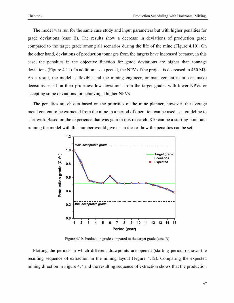
Chapter 4 Production Scheduling with Horizontal Mixing
67
The model was run for the same case study and input parameters but with higher penalties for
grade deviations (case B). The results show a decrease in deviations of production grade
compared to the target grade among all scenarios during the life of the mine (Figure 4.10). On
the other hand, deviations of production tonnages from the targets have increased because, in this
case, the penalties in the objective function for grade deviations are higher than tonnage
deviations (Figure 4.11). In addition, as expected, the NPV of the project is decreased to 450 M$.
As a result, the model is flexible and the mining engineer, or management team, can make
decisions based on their priorities: low deviations from the target grades with lower NPVs or
accepting some deviations for achieving a higher NPVs.
The penalties are chosen based on the priorities of the mine planner, however, the average
metal content to be extracted from the mine in a period of operation can be used as a guideline to
start with. Based on the experience that was gain in this research, $10 can be a starting point and
running the model with this number would give us an idea of how the penalties can be set.
Figure 4.10. Production grade compared to the target grade (case B)
Plotting the periods in which different drawpoints are opened (starting periods) shows the
resulting sequence of extraction in the mining layout (Figure 4.12). Comparing the expected
mining direction in Figure 4.7 and the resulting sequence of extraction shows that the production

Chapter 4 Production Scheduling with Horizontal Mixing
68
schedule follows the desired mining direction in addition to satisfying the number of active
drawpoints constraint (Figure 4.13). The BHOD and as a result, the mining reserve is calculated
as one of the outputs of the production schedule. Figure 4.14 shows the BHOD for draw columns
compared to their initial heights. Additionally, the mineral reserve can be determined according
to the BHODs as an output of the production scheduling optimization.
Figure 4.11. Ore production during the life of the mine (case B)
Figure 4.12. Sequence of extraction for drawpoints based on the defined mining direction

Chapter 4 Production Scheduling with Horizontal Mixing
69
Figure 4.13. Number of active drawpoints during the life of the mine
Figure 4.14. Height of draw columns after extraction compared to their initial height
4.5. Summary
Despite its significant impact on production scheduling, material flow and its uncertainties
have not been part of production scheduling models. These uncertainties can cause gaps between
the production goals and actual operations resulting in an inefficient mine to mill system. In this

Chapter 4 Production Scheduling with Horizontal Mixing
70
chapter, using stochastic optimization, an MILP model was proposed to capture the horizontal
mixing that occurs in material flow when extracting from drawpoints in block-cave mining.
Adjacent slices located in the same neighborhood were used to generate scenarios in order to
simulatethehorizontalmovementsofmaterial.Toaddresstheprocessingplant’sobjectives,in
addition to technical and operational constraints, the model was built based on two production
targets: tonnage and grade. For the presented case study, the resulting tonnages show only minor
deviations from the targets in all scenarios and there are visible deviations between the target
grade and the resulting production grade which is mainly because of the defined mining
direction. The BHOD calculation was also brought into the optimization, which means that the
mineral reserve is the output of the production scheduling and not an input; this takes us one step
closer towards overall optimization. The model was run for two different sets of penalties for
grade deviations and it was shown that increasing the penalties will provide us with closer results
to the targets but most probably lower NPVs. As a result, mine planners can use the proposed
stochastic optimization model as a flexible tool by setting the penalties for deviations of
production from their specified targets based on their priorities: higher penalties will result in
low deviations from the targets but probably lower NPVs, and vice versa. In the next chapter, the
model is more developed to include both vertical and horizontal mixing in the production
scheduling and then it is validated against a commercial software.

71
Chapter 5 Long-term Production Scheduling Optimization and 3-D
Material Mixing Analysis for Block Caving Mines
Chapter 5 presents block caving production scheduling optimizer, BCSO, in which the NPV is
maximized and deviations from target grades and tonnages are minimized for all scenarios
during the life of the mine. Cone of Movement, CoM, is introduced in order to take horizontal
and vertical mixing into consideration for production scheduling optimization. The BCSO is
tested for a block caving mine and then the results have been validated against GEOVIA PCBC
software.
A version of this chapter has been submitted to Mining Technology (TIMM A) and it is under review:
Khodayari F, Pourrahimian Y. 2018. Long-term production scheduling optimisation and 3-D material
mixing analysis for block caving mines. Mining Technology (TIMM A), © IOM3, (Under review, 18
pages, July 2018).

Chapter 5 Long-term Production Scheduling with 3D Material Mixing
72
5.1. Introduction
For production planning purposes, similar to blocks in open-pit mining, ‘slices’ are the
decision units in block caving; the height of a slice is usually equal to the height of one block in
the block model, and its area depends on the geometry of drawpoints in the layout (Figure 5.1).
Similar to a block, each slice is represented by its grade, density, volume, and other properties
as needed.
Figure 5.1. Block model (on the left), drawpoints and slice model (on the right)
Since the rock is fractured and moved into drawpoints by gravity, operating cost in block
caving is lower than other underground mining methods. However, long periods of development
requires high capital costs and this is one of the main challenges of this method; therefore, a
practical production schedule with the possibility of generating higher revenues earlier in the
project can significantly improve the cash flow of the project and change a deep low-grade ore
resource to a valuable ore reserve.
As the caved rock flows down into drawpoints, different types of mixing occur mainly
because of the diverse sizes and velocities of particles. This mixing can result in dilution and
changes in the grades and tonnages extracting from drawpoints, drawpoint must be shut down if

Chapter 5 Long-term Production Scheduling with 3D Material Mixing
73
dilution is more than the acceptable limit. Therefore, production scheduling in block caving
should take into account the material mixing and its impact on the production as a whole.
Although very useful, most of the current optimization models do not incorporate the
material flow, the mixing that occurs in the caved material within the draw columns, and its
uncertainties in the production schedule. Khodayari and Pourrahimian (2017) used stochastic
optimization to include horizontal mixing in the production scheduling model. In their
methodology, the model generates a series of scenarios based on the grade distribution in
each draw column and the slices in the neighborhood of each drawpoint. In this chapter, the
new version of this optimization model is presented in which 3-D mixing, including vertical and
horizontal movements, of caved rock within drawpoints is considered. Scenarios are defined for
both production grades and tonnages to analyze the impact of mixing on the production schedule
and propose more reliable plans compared to the existing models.
PCBC (Personal Computer for Block Caving) software is used almost by all mining
companies working in block caving across the world (DassaultSystèmes 2018). Constructing the
slice model, calculation of the best height of draw (BHOD) for drawpoints, implementation of
mixing algorithms, finding a footprint, and production schedule optimization are the main
features of this software. The software has been in use for more than 30 years, it was developed
by Gemcom Software International Inc. and now is owned by Dassault Systèmes (Diering 2013).
Because of the reputation of GEOVIA PCBC, it was chosen for validation of BCSO.
In the following sections, first the methodology that is used for developing the BCSO is
explained and formulations of the mathematical programming model are presented, then a real
block caving mine is used to test the proposed prototype. In the next step, 3 cases are considered
to run the BCSO as well as to generate production schedules using PCBC. Additionally, another
case is run by the BCSO to test the target grade option as one of its features, this case is not
compared with PCBC because it does not offer this application. Finally, the results are discussed.
5.2. Methodology
5.2.1. 3-D Mixing
The goal is to generate a series of scenarios that can provide us with an understanding
of movements of caved rock within a draw column and its neighbors based on the slice model, as

Chapter 5 Long-term Production Scheduling with 3D Material Mixing
74
the material is extracted from drawpoints. For each step of draw from a drawpoint, when a slice
is extracted, an open space is available that can be filled by the slices above and in the
neighborhood. These candidate slices fall into a three-dimensional space called Cone of
Movement (CoM). Based on the geometry of drawpoints and the caving propagation, the shape
is a cone (Laubscher 1994). To understand the scale in which particles can move within the
caved area, researchers have used theoretical, experimental (pilot and full-scale), and numerical
analysis (Sun et al. 2018).
As a numerical example, Pierce (2010) developed a model to study the gravity flow; he
proposed some formulations to predict the particle movements and resulting dilution.
Application of these equations requires a lot of information about rock properties and caving
operations and is limited to certain conditions. On the other hand, in a full-scale experiment at
the El Teniente block caving mine, Alvial (1992, as cited in Laubscher (2000)) concluded that
horizontal displacement (HD) can range between 2 and 42 meters and vertical slip angle (VSA)
can vary from 60 to 80 degrees. Although this study was carried out long time ago, these ranges
can provide an invaluable guideline to include caving flow into production planning. Since the
focus of this research is optimization of long-term production schedule, the proposed ranges by
Alvial are used to define the CoM. Figure 5.2 shows an example of a single CoM and how
different CoMs located in the same neighborhood can overlap with each other. As it can be seen,
a CoM is represented by its HD and VSA.
Figure 5.2. Cone of Movement (CoM) and the overlap between CoMs in the same neighborhood
When a slice is extracted from a drawpoint, we can imagine that a void space is formed at
the entrance of the drawpoint that can be filled by the other slices located in the CoM

Chapter 5 Long-term Production Scheduling with 3D Material Mixing
75
(Figure 5.3). Although the probabilities to fill the void space for each of those slices in the CoM
are different, it is almost impossible to calculate the exact probabilities. Instead, all of the slices
in the CoM are considered to generate a series of scenarios of grade and tonnage to be
implemented in the optimization model. Therefore, the resulting production schedule takes into
account the flow of material within the caved area, and this leads us to more reliable mine plans.
An illustrative example of how the grades of slices in the CoM are used to generate the scenarios
is presented below.
Figure 5.3. Candidate slices that are located in the CoM (yellow balls)
Equation (5.1) shows the first step where a " "Set of candidate slices that fall into the CoM is
formed, " "ag is grade for individual slices in the CoM and " "A is number of candidates (slices).
Let us suppose that for an available void space above a drawpoint, a CoM is formed that contains
20 slices and based on the resource model, the grades of these slices are used to form the set
(Table 5.1).
1 = ,..., ASet g g (5.1)
Table 5.1. The set of grades for the candidate slices in the CoM (illustrative example)
Slices 1 to 10 1.31 1.18 1.18 1.18 1.09 1.15 1.08 1.12 0.98 1.21
Slices 11 to 20 0.90 1.18 0.91 1.00 1.46 1.40 1.41 1.50 1.35 1.42

Chapter 5 Long-term Production Scheduling with 3D Material Mixing
76
Then, " "N random grades are generated based on the set of candidates as it is shown in
equation (5.2), where " "N is number of scenarios. In this example, 10 scenarios are generated
(Table 5.2).
( ) 1,..., n RandSample Setg n N (5.2)
Table 5.2. The generated scenarios (illustrative example)
Scenario # 1 2 3 4 5 6 7 8 9 10
Grade (%) 1.40 1.12 1.09 0.98 1.18 1.18 1.35 1.42 1.18 1.18
It should be noted that in this research, as the smallest units in the model, slices are considered
to generate the population and the scenarios.
5.2.2. Optimization Model
In this section, first the notations that are used in this chapter are introduced and then the
objective function and constraints of the model are discussed.
Notation
Indices
{1,..., }t T Index for scheduling periods.
{1,..., }s S Index for individual slices.
{1,..., }d D Index for individual drawpoints.
{1,..., }n N Index for individual scenarios.
{1,..., }a A Index for adjacent drawpoints, " "A is number of slices that are located in
the same neighborhood.
Variables
,s tx
Binary decision variable that determines if slice " "s is extracted in period
" "t (, 1s tx ) or not (
, 0s tx ), for each slice one decision variable is
considered.
,d ty
Binary decision variable which determines whether drawpoint " "d in
period " "t is active (, 1d ty ) or not (
, 0d ty ), one decision variable for
each drawpoint.

Chapter 5 Long-term Production Scheduling with 3D Material Mixing
77
,d tz
Binary decision variable determining whether drawpoint " "d at period " "t
has started its extraction (, 1d tz ) or not (
, 0d tz ), one decision variable
for each drawpoint.
, [0, ) uo
n tdev Continuous decision variable representing excessive amount from the
target production ore in scenario " "n at period " "t .
, [0, ) lo
n tdev Continuous decision variable representing deficient amount from the target
production ore in scenario " "n at period " "t .
g
, [0, ) u
n tdev Continuous decision variable representing excessive amount from the
target production grade (the metal content) in scenario " "n at period " "t .
g
, [0, ) l
n tdev Continuous decision variable representing deficient amount from the target
production grade (the metal content) in scenario " "n at period " "t .
Model Parameters
e
sg Grade of element " "e for slice " "s .
,n s Density of slice " "s (t/m3) for scenario " "n .
sV Volume of slice " "s (m3).
t
Current period, this notaion is used for defining ," "d tz , it represents
periods 1 up to the period that the constraint is calculating for.
SdN Number of slices in draw column" "d that are located above drawpoint" "d .
pd
Drawpoint that its extraction should be started before drawpoint " "d based
on the defined mining direction.
ps
Index for the slice that is a precedence for slice " "s , " "ps represents the
slices that are located below " "s in the same draw column and must be
extracted before slice " "s .
Input Parameters
ˆ e
tg Target production grade for element " "e in period" "t , which is defined
based on the production goals and processing requirements.

Chapter 5 Long-term Production Scheduling with 3D Material Mixing
78
,s to Ore production resulting from extraction slice " "s in period" "t .
ˆto
Target ore production in period " "t which is defined based on the
production goals and processing requirements.
min tAct Minimum number of active drawpoints in period " "t .
max tAct Maximum number of active drawpoints in period " "t .
M
A big number, this is chosen based on the maximum number of slices in
draw columns.
minDL Minimum drawpoint life.
maxDL Maximum drawpoint life.
minDR Minimum draw rate (tonne per period).
maxDR Maximum draw rate (tonne per period).
i Discount rate.
Ramp up Ramp-up time used for production goals.
ScenNum Number of scenarios.
,d tDP Drawpoint depletion percentage: the portion of draw column associated
with drawpoint " "d that has been extracted from '1 t to t t .
ep Price of element " "e ($/tonne).
c Operating costs ($/tonne). loc Cost (penalty) for deficient amount of ore production from the targets ($).
uoc Cost (penalty) for excessive ore production from the targets ($).
lgc Cost (penalty) for deficient production grade from the targets ($).
ugc Cost (penalty) for excessive production grade from the targets ($).
er Recovery of the processing plant for element " "e (%).
Objective function
The objective function is defined as follows:

Chapter 5 Long-term Production Scheduling with 3D Material Mixing
79
, , , ,
1 1 1 1 1 1
{( )} { } { }
T S T N T N
s t s t n t n t
t s t n t n
Maximize E NPV x Ore deviations Grade deviations
, ,
,
1 1 1
lg lg g
n, , n, ,
1 1 1 1
1
(1 )
1 1
(1 ) (1 )
e e eT S N
n s n s s
s ttt s n
lo lo uo uo ug uT N T Nt n t t n t
t tt n t n
p r g c Vx
N i
c dev c dev c dev c dev
N i N i
(5.3)
Equation (5.3) maximizes the NPV of the project for the life of the mine (the first part) while
minimizes the deviations of production tonnages and production grades for all mixing scenarios
(the second part). The calculated NPV is based on the generated mixing scenarios resulting from
the caving flow. The decision variables in the production scheduling model are based on slices,
and the resulting solution determines the slices to extract from each draw column and the time in
which they should be extracted. This will improve flexibility of the operations by providing the
mining engineers with a detailed plan to follow in order to achieve the production targets and the
maximum NPV for the life of the mine.
The mine planer makes the decision about the penalties (clo
, cuo
, c
lg, c
ug) for deviations from
the targets ( ˆto , ˆ e
tg ); depends on the company’s priorities, higher penalties will result in lower
deviations but potentially longer computational time and lower NPVs; also, it is expected to
achieve higher NPVs and to spend less time for solving the problem when choosing lower values
for the penalties. Number of scenarios is a factor of mixing in the caved zone above drawpoints,
for example, more mixing scenarios should be considered for a more diverse range of particles
with different sizes and as a result different velocities.
Constraints
First, we should define some relations between the decision variables that represent
drawpoints and the ones that represent slices, in other words, we need to know whether any
slices are extracted from drawpoint " "d in period " "t , which means checking the status of the
drawpoint to see if it is active or not in each period. Equation (5.4) and (5.5) present such a
relationship in which " "x and " "y decision variables are connected.

Chapter 5 Long-term Production Scheduling with 3D Material Mixing
80
, ,
1
0 1,..., , 1,...,
SdN
d t s t
s
y M x d D t T (5.4)
, ,
1
0 1,..., , 1,...,
SdN
s t d t
s
x M y d D t T (5.5)
Using these equations, we can control the number of drawpoints that can be active in each
period; this is done in equation (5.6) and helps the mine manager to plan ahead for equipment
selection and also the allocation of resources in the operations.
,
1
min max 1,...,
D
t d t t
d
Act y Act t T (5.6)
We also introduce a new set of decision variables called " "z that makes it possible to not
only implement the precedence of extraction among drawpoints within the layout but also to
maintain a continuous production during the life of the mine, as it has been shown in equations
(5.7), (5.8), and (5.9).
, ,
1
1,..., , 1,...,t
d t d t
t
DP y d D t T
(5.7)
, , 1,..., , 1,..., d t d tDP M z d D t T (5.8)
, , 1,..., , 1,..., d t d tz M DP d D t T (5.9)
where " "t is the current period that the model is monitoring and this has to be done for all
periods ( ' 1,...,t T ). In each period, ," "d tz , which is a binary decision variable, is 1 if
drawpoint " "d has been opened in periods before or at '" "t and 0 if not. Continuous
production is critical in block caving for preventing compaction and its consequences, means that
if a drawpoint starts its extraction, then it is kept open until its life is over and it will not be active
after closure. Equation (5.10) guarantees a continuous production during the life of the mine.
, , 1 ,(1 ) 1,..., , 1,..., d t d t d ty y z d D t T (5.10)

Chapter 5 Long-term Production Scheduling with 3D Material Mixing
81
To define the precedence of drawpoints, a proper mining direction within the designed layout
should be defined. Khodayari and Pourrahimian (2015a) proposed a methodology that finds the
mining direction based on the dollar values of the metal content in draw columns. When the
precedence of drawpoints is determined using this technique, equation (5.11) can implement the
precedence between drawpoints in the optimization model and makes sure that the desired
mining direction is followed during life of the mine. Since in PCBC this procedure is done
manually, the input precedence for PCBC can be provided by the BCSO for achieving higher
NPVs. This is shown in the case study later in this chapter.
, , 1,..., , 1,..., pd t d tz y d D t T (5.11)
In addition to the precedence between drawpoints, slices should be extracted based on a
precedence that is defined using their vertical locations in draw columns; in other words, a slice
cannot be extracted from a drawpoint unless all slices located below (in the same draw column)
are already extracted. This vertical precedence is formulated by equation (5.12).
, ,
1
1,..., , 1,...,p
t
s t s t
t
x x d D t T
(5.12)
Two constraints are added to minimize production deviations from targets (tonnage and
grade). Equations (5.13) and (5.14) are two soft constraints that keep the production tonnages
and production grades as close as possible to the targets in all scenarios.
,,
1
ˆ 0 1,..., , 1,...,
lo uo
s s t t n n
S
s n
s
V x o dev dev n N t T (5.13)
lg,, ,
1
) 0 1,..., , 1,...,ˆ(
e ugt s s t n n
S
s n s n
s
V x dev dev n N t Tg g (5.14)
Extraction per year from individual drawpoints or draw rate, and life of drawpoints (draw life)
are two other criteria that have to be considered for developing a practical production schedule.
These are limited by factors such as availability of mining equipment, geotechnical conditions of
the orebody and the host rock, geometry of drawpoints, and height of draw columns. Equations

Chapter 5 Long-term Production Scheduling with 3D Material Mixing
82
(5.15) and (5.16) control draw rate and draw life as two of the constraints for the optimization
model.
, ,
1
1,..., , 1,...,
ds
min d t s s s t max
s
DR y V x DR d D t T (5.15)
min , max
1
1,...,
T
d t
t
DL y DL d D (5.16)
Finally, we have to make sure that the mineral reserve, which is the total tonnage resulting
from the production schedule, is less than or equal to the mineral resource (the input model to the
production schedule). This is implemented in the model using equation (5.17).
,1
1,...,1 T
s tt
Sx s
(5.17)
5.2.3. Model Structure and Programming Tools
As it was presented above, the optimization model consists of three sets of decision variables:
(1) binary variables that represent slices, size of this set is equal to total number of slices in the
original reserve model multiplied by the scheduling periods, (2) binary variables that represent
drawpoints, size of this set is equal to number of drawpoints multiplied by periods of scheduling,
(3) continuous variables representing mixing scenarios, its size is a multiplication of number of
scenarios by the scheduling periods.
The model was coded in MATLAB (TheMathWorksInc. 2017) and is solved by calling
CPLEX solver (IBM 2017) through MATLAB. CPLEX solves the optimization problem using
branch-and-cut in which a search tree with a series of nodes is created where each node
represents an LP subproblem. Nodes are analyzed until no more active nodes are available or
some limit has been reached (IBM 2017).
5.3. Verification and Validation
To verify the BCSO, it is tested on a real case block caving mine. The mineral resource
contains 220.5 million tonnes of ore with the average grade of 0.86% copper. The mine is
planned to be operated in a layout of 424 drawpoints (Figure 5.4); the slice model is created in

Chapter 5 Long-term Production Scheduling with 3D Material Mixing
83
PCBC using the original block model with the block height of 20 meters (Figure 5.5), copper
grade and ore tonnage distributions for slices in the slice model are presented in Figure 5.6 and
Figure 5.7.
As it was already mentioned in section 5.2.2, the mining direction dictates the precedence of
extraction among drawpoints and it is chosen based on economic and geomechanical
considerations. In this case study, we assume that economic parameters are drivers for making
such a decision. Therefore, the methodology proposed by Khodayari and Pourrahimian (2015) is
used to find the mining direction. Figure 5.8 shows that the best direction would be starting from
the south side of the deposit, then moving towards the center and finishing in the north east of
the layout. As a result, a V-shape direction with the starting coordination of (100, 1050), ending
coordination of (600, 1650), and V-shape angle of 150 degrees is considered. This mining
direction and the resulting optimal precedence of extraction for drawpoints, which is generated
by the BCSO, is used as an input for this case study in PCBC. This procedure is manual in PCBC
and the precedence is given by the user. However, in this research, the precedence is generated
by the BCSO and as a result, higher NPVs are expected even for the resulting schedule from
PCBC.
Figure 5.4. Layout of drawpoints

Chapter 5 Long-term Production Scheduling with 3D Material Mixing
84
Figure 5.5. The created slice model in PCBC (Scale: 1:5000)
Figure 5.6. Distribution of copper grade for slices in the slice model

Chapter 5 Long-term Production Scheduling with 3D Material Mixing
85
Figure 5.7. Distribution of tonnage for slices in the slice model
Figure 5.8. Desired mining direction in the drawpoint layout
The input scheduling parameters are presented in Table 5.3. The target grade is only used for
the last case, where the target grade feature of BCSO is tested and will be discussed later in this
chapter.

Chapter 5 Long-term Production Scheduling with 3D Material Mixing
86
Table 5.3. Scheduling parameters for the case study
Parameter Value Unit Description
T 10 Year Production scheduling timeline (the life of the mine).
ˆ cu
tg 1 % Target production grade for copper (Cu) 1,..., t T .
1o 8 Mt Ore production target in the first year of production.
2o 16.5 Mt Ore production target in the second year of production.
ˆto 25 Mt Ore production target for operating in the full capacity 3,..., t T .
Ramp-up
time 3 Year
The time in which the production is increased from starting amount to the
full capacity.
MIP gap 1 % Relative tolerance on the gap between the best integer objective and the
objective of the best node remaining.
DRmin 0 tonne/year Minimum draw rate.
DRmax 100,000 tonne/year Maximum draw rate.
pcu
6,500 $/tonne Copper price.
c 23 $/tonne Operating costs of ore (Mining + Processing).
i 10 % Discount rate.
rcu
85 % Recovery of the processing plant for copper (Cu).
N 10 - Number of scenarios.
M 100 - M must be greater than the maximum number of slices for an individual
drawpoint (sdN ), the maximum
sdN for this case study is 36.
HD 30 meter Horizontal Displacement.
VSA 60 degree Vertical Slip Angle.
Production schedules are generated using the BCSO and PCBC. To have a thorough
comparison and discussion, different cases are considered based on the flexibility of both tools.
In all of the following cases, constraints for precedence of drawpoints, precedence of slices,
continuous mining, and reserve are included and satisfied as part of the optimization. The three
cases are as follows:
Case (1): this is the base case to see how much the ore reserve could be if there are no
limitations for the draw rate, mixing is not considered,
Case (2): a draw rate limit of 100,000 tonnes per year is added to the constraints, mixing is
not involved,
Case (3): in addition to a draw rate limit of 100,000 tonnes per year, 10 mixing scenarios are
generated using the 3-D CoM and included in the BCSO. In PCBC, the Template Mixing tool is
used in the production scheduling.
Chapter 5 Long-term Production Scheduling with 3D Material Mixing
87
For PCBC, three different scheduling methods (AUTO, SMOOTH, and COMBO) were used:
AUTO extracts the maximum tonnages allowed by the production rate curve (draw rate
constraint) for each drawpoint to achieve the required tonnage (target tonnage). The tonnages for
the remaining active drawpoints will be set to 0 and those drawpoints are flagged as idle. In case
of too many idle drawpoints in different periods, using the AUTO method is probably
inappropriate (DassaultSystèmes 2018). SMOOTH is an extension to AUTO while in this
method when idle drawpoints are encountered, the tonnage will be increased linearly between the
most newly opened drawpoints and the older ones to make sure that there are no idle drawpoints
(DassaultSystèmes 2018). COMBO takes the total requested tonnage and divides it among all
active drawpoints in the proportion of the amount of material remaining in each draw column.
Higher columns are drawn faster than columns with less material. In this method, all drawpoints
are active in all periods during the life of the mine while the maximum draw rate constraint is
satisfied (DassaultSystèmes 2018).
Table 5.4 summarizes the results for the production schedules generated by the BCSO and
different methods under PCBC. Some of the findings are explained below:
Results show that for case (1), both the BCSO and PCBC extract the whole mineral
resource (220.5 million tonnes of ore) during the life of the mine (10 years), turning the whole
mineral resource to mineral reserve. However, the BCSO can improve the NPV of the project for
the same amount of production by 4%, 6%, and 11% compared to the AUTO, SMOOTH, and
COMBO methods in (Figure 5.9). For all of these methodologies, the solution (computational)
time was less than one minute.
In case (2), adding the draw rate constraint, as it was expected, has resulted in
smaller mineral reserves and lower NPVs; a total production of 215.25 and 201.32 million tonnes
of ore are planned by the BCSO and PCBC AUTO while BCSO generates a higher NPV (+2%).
The NPV for SMOOTH is similar to that of AUTO but with higher tonnages (204.5 million
tonnes) to extract, and COMBO suggests a mineral reserve of 216 million tonnes with the lowest
NPV (Figure 5.10). Also, it took less than one minute to solve the problem using the BCSO or to
generate a production schedule in PCBC.
Case (3) includes material mixing into the production scheduling. Results show that
the total tonnage and NPV reduce for the proposed production schedule from the BCSO and

Chapter 5 Long-term Production Scheduling with 3D Material Mixing
88
the generated schedule in the PCBC. The total tonnage and NPV for the BCSO are 198.9
million tonnes and $3.4 billion while these values for PCBC AUTO are 192.4 million tonnes and
$3.27 billion (Figure 5.11). The BCSO has suggested a mine plan with a higher NPV (+ 4%)
compared to the AUTO. Similar to case (2), SMOOTH has generated the same NPV but higher
tonnage (197 Mt) compared to the AUTO method. Moreover, COMBO generates the highest
tonnage (199 Mt) but lowest NPV ($3.12 billion). Incorporation of mixing adds to complexity of
the scheduling problem and as a result, the solution time increases.
For testing the target optimizer feature in the BCSO, a target grade of 1% was set for the same
block caving mine. In this case, ten mixing scenarios were considered within the scheduling, and
the objective function’s goal was to maximize the NPV while minimizing deviations of
production grades from the desired target grade in all scenarios. A cost of $20 was assumed as
the penalty for excessive or deficient production grades from the target grade. This assumption
can change based on priorities of the mine planner; lower values for deviations and NPV is
expected for higher penalty rates, and vice versa. Figure 5.12 shows that production grades in
different scenarios are significantly close to the target grade during the life of the mine. In this
case, the ‘AverageScen’ represents the average values calculated based on all scenarios. This
case has not been compared with the PCBC because it does not offer such a feature that target
grades could be set.
Table 5.4. Comparison of the results
Description Method Total Tonnage (Mt) NPV (B$) NPV Dif.
Case (1):
No mixing
No draw rate constraint
BCSO 220.5 3.59 0%
PCBC (AUTO) 220.5 3.46 - 4%
PCBC (SMOOTH) 220.5 3.4 - 6%
PCBC (COMBO) 220.5 3.24 - 11%
Case (2):
No mixing
With draw rate constraint
BCSO 215.25 3.5 0%
PCBC (AUTO) 201.32 3.4 - 2%
PCBC (SMOOTH) 204.5 3.4 - 2%
PCBC (COMBO) 216 3.2 - 8%
Case (3):
With mixing
With draw rate constraint
BCSO 198.9 3.4 0%
PCBC (AUTO) 192.4 3.27 - 4%
PCBC (SMOOTH) 197 3.28 - 4%
PCBC (COMBO) 199 3.12 - 9%

Chapter 5 Long-term Production Scheduling with 3D Material Mixing
89
Figure 5.9. Production tonnages and grades for case (1)
Figure 5.10. Production tonnages and grades for case (2)

Chapter 5 Long-term Production Scheduling with 3D Material Mixing
90
Figure 5.11. Production tonnages and grades for case (3)
Figure 5.12. Resulting BCSO production grade based on a target copper grade of 1% for 10 scenarios

Chapter 5 Long-term Production Scheduling with 3D Material Mixing
91
5.4. Summary
In this chapter, a stochastic optimization model was presented that incorporates material
mixing in the production scheduling optimization, the prototype software application with a
graphical interface is called block caving production scheduling optimizer (BCSO). The
proposed model was tested against PCBC, as the commercial software which has been developed
and used during the past 30 years. Based on the available features of the PCBC, different cases
were studied to carry out production scheduling for a block caving mine. This chapter’saimwas
to introduce and validate the BCSO by testing this prototype against a commercial software with
a high reputation such as PCBC. For a block caving mine of 424 drawpoints, the resulted
production schedules were close; however, the BCSO generates higher NPVs for all three cases
that were studied. The solution times were reasonable and significantly close for cases (1)
and (2), but it took longer for BCSO to run case (3) when the mixing was added to the problem.
Due to the limitations of PCBC for using different constraints in the scheduling, only 6 (out of 9)
existing constraints in the BCSO were used for the comparison purposes. The prototype has
more to offer and it is flexible in terms of adding new constraints based on the specifications of
the mining project. The precedence of drawpoints based on advancement direction, which is an
input to production scheduling, is traditionally chosen manually by the user. However, in this
research, the precedence was generated by the BCSO using an automated method. Then the
obtained optimal precedence of extraction from BCSO was used as an input for scheduling in
PCBC instead of manual methods. In addition, the target grade option embedded in the BCSO
was tested for situations where the processing plant is limited to be fed by a certain ore grade. It
was shown that the desired production grade could be achieved during the life of the mine by
activating the target grade option in the BCSO. In this case, PCBC was not used for comparison
because it does not offer such a feature. Incorporating mixing and considering its impact on the
production helps us to achieve more reliable mine plans for block caving; the developed
prototype uses the CoM concept to take into account material mixing within the caving flow in
the production scheduling optimization in addition to the ability to satisfy the operational
constraints in the block-cave mining.

92
Chapter 6
Conclusions and Recommendations
Chapter 6 provides key conclusions from this research and some recommendations for future
studies.

Chapter 6 Conclusions and Recommendations
93
This study presents a mathematical programming model that optimizes the production
schedule in block caving during the life of the mine. The model was verified based on real-case
data from block caving operations and validated against the current practice in the mining
industry.
6.1. Conclusions
The key conclusions from this study can be summarized under the following points:
An optimum production schedule can significantly add to the dollar values of a mining
project. As a strong tool, mathematical programming can be used to optimize the
production schedule for block caving; it can generate practical plans by satisfying
technical constraints of the operations and determine how far the final solution is from
the optimal one by reporting the optimality gap in case of integer programming.
Caving flow and the resulting mixing impacts the production and it should be included
in the production scheduling optimization. CoM provides a good perspective about
materialflowandtheprobabilitiesofparticles’movementswithindrawcolumns.
The proposed block caving scheduling optimizer, BCSO, incorporates mixing into
production scheduling while maximizing the NPV of the project and satisfying the
technical constraints. While being capable of modeling more constraints for the caving
operations, it can offer higher NPVs compared to commercial tools such as PCBC.
Using the BCSO, different mixing scenarios can be generated to capture the probable
material flow within the caving zone. In the resulting production schedule, the target
production grades and tonnages are achieved for all scenarios during the life of the
mine while the defined limitations are satisfied.
The mixing tool in BCSO requires a minimum level of information about the caving
flow and is useful for long-term production scheduling purposes, where many
parameters are unknown. On the other hand, mixing template tool in PCBC is
dependent on input parameters that require a higher level of information that could
only be available during operations.
The precedence of drawpoints based on advancement direction, which is an input to
production scheduling, is traditionally chosen manually by the user. However, the
Chapter 6 Conclusions and Recommendations
94
precedence can be generated by the BCSO using an automated method. Then the
resulting precedence of extraction from BCSO can be used as an input for scheduling
in PCBC instead of results of manual methods.
The BCSO is a flexible scheduling tool in which more technical constraints, based on
the specifics of the mining operations, can be added to the existing constraints in the
current optimization model.
Dependingontheminingcompany’sstrategicplan,new targets with different levels
of priorities can be included in the scheduling, the BCSO uses the penalties as
prioritizing factors to minimize deviations of the final production schedule from the
targets.
6.2. Recommendations
In this study, several simplifying assumptions were made for the caving flow and mixing, the
technical limitations of the operations, the price, the cost, and production targets. To address
these limitations, the following points are recommended as possible directions for future studies.
The caving flow and its resulting mixing could be looked at in more details and a more
developed version of CoM can be used to include in the BCSO. However, it should be
noted that the caving flow could be case-specific and such level of detail is not usually
available for long-term planning unless production has started and drawpoints are
monitored for a long time.
More technical constraints can be added to the BCSO based on the specifics of the
mining project such as: geometry,equipment, company’s limitations, final product’s
market, and processing plant.
The price and cost were assumed to not change during the life of the mine, other
approaches such as variable price and cost for each year based on the forecasts can be
considered. Also, uncertainties of price and cost can be included in the model.
Only production grades and tonnages are included for targets in the current model,
othertargetsbasedonthemarketdemand,processinglimitations,andthecompany’s
strategic plan can be added to the model.

Chapter 6 Conclusions and Recommendations
95
Since the proposed model is valid for long-term production scheduling, it is
recommended to consider the short-term production scheduling for a real-case block
caving operations and study the practicality of transition from long-term to short-term
planning.
It is recommended that to investigate the possibility of consideration of uncertainties
of the caving flow in a dynamic model in which the impact of production on the flow
can simultaneously be studied.
Consideration of the total tonnages and weighted grades of draw columns for the
mining direction finder can be a limitation of this methodology; application of other
approaches can be studied to improve this feature of the model.

96
References
[1] Alonso-Ayuso A, Carvallo F, Escudero LF, Guignard M, Pi J, Puranmalka R, Weintraub
A. 2014. Medium range optimization of copper extraction planning under uncertainty in
future copper prices. European Journal of Operational Research. 233(3):711-726.
[2] Bergen D, Rennie W, Scott C. 2009. Technical Report on the New Afton Project, British
Columbia, Canada. New Gold Inc., Vancouver, British Columbia. 1416.
[3] Brown ET. 2003. Block caving geomechanics. Indooroopilly, Queensland: Julius
Kruttschnitt Mineral Researh Centre, The University of Queensland.
[4] Brown ET. 2007. Block caving geomechanics. Indooroopilly, Qld.: Julius Kruttschnitt
Mineral Research Centre, The University of Queensland.
[5] Brunton I, Lett J, Sharrock G, Thornhill T, Mobilio B. 2016. Full Scale Flow Marker
Experiments at the Ridgeway Deeps and Cadia East Block Cave Operations. Massmin
2016; May 9-11; Sydney, Australia.
[6] Carter PG. 2011. Chapter 6.3, Selection Process for hard-Rock Mining. In: Darling P,
editor. SME mining engineering handbook [electronic resource]. 3 ed. [Englewood, Colo.]
: Society for Mining, Metallurgy, and Exploration, c2011.; p. 357-376.
[7] Castro R, Gonzalez F, Arancibia E. 2009. Development of a gravity flow numerical model
for the evaluation of drawpoint spacing for block/panel caving. Journal of the Southern
African Institute of Mining and Metallurgy. 109(7):393-400. English.
[8] Castro RL, Fuenzalida MA, Lund F. 2014. Experimental study of gravity flow under
confined conditions. International Journal of Rock Mechanics and Mining Sciences.
67:164-169.
[9] Chanda E, Dagdelen K. 1995. Optimal blending of mine production using goal
programming and interactive graphics systems. International Journal of Surface Mining,
Reclamation and Environment. 9(4):203-208.
[10] Chanda ECK. 1990. An application of integer programming and simulation to production
planning for a stratiform ore body. Mining Science and Technology. 11(2):165-172.
[11] Dagdelen K, Johnson TB. 1986. Optimum open pit mine production scheduling by
lagrangian parameterization. 19th Application of Computers and Operations Research in
the Mineral Industry Proceedings; April 14 to 18; Pennsylvania, USA.
[12] DassaultSystèmes. 2018. GEOVIA PCBC Version 6.7.
[13] Diering T. 2000. PC-BC: A Block Cave Design and Draw Control System. Massmin
2000; Oct 29 to Nov 02; Brisbane, Australia.
[14] Diering T. 2004. Computational considerations for production scheduling of block cave
mines. MassMin 2004; Aug 22-25; Santiago, Chile.
[15] Diering T. 2012. Quadratic Programming applications to block cave scheduling and cave
management. Massmin 2012; June 10-14, 2012; Sudbury, Ontario, Canada.
[16] Diering T. 2013. Ore Reserve estimation for Block Cave Mines Using GEOVIA PCBC.
White Paper.

References
97
[17] Dirkx R, Dimitrakopoulos R, Kazakidis V. 2018. Stochastic optimisation of long-term
block cave scheduling with hang-up and grade uncertainty. International Journal of
Mining, Reclamation and Environment.1-18. English.
[18] Dorador L, Eberhardt E, Elmo D, Aguayo A. 2014. Influence of secondary fragmentation
and column height on block size distribution and fines migration reaching drawpoints. 3rd
International Symposium on Block and Sublevel caving (CAVING 2014); Jun 5-6;
Santiago, Chile.
[19] Eadie B. 2002. A framework for modelling fragmentation in block caving [Ph.D.]. Julius
Kruttschnitt Mineral Research Centre: The University of Queensland.
[20] Eiselt HA, Sandblom CL. 2010. Operations Research (A Model-Based Approach).
Springer Berlin Heidelberg.
[21] Epstein R, Goic M, Weintraub A, Catalán J, Santibáñez P, Urrutia R, Cancino R, Gaete S,
Aguayo A, Caro F. 2012. Optimizing Long-Term Production Plans in Underground and
Open-Pit Copper Mines. Operations Research. 60(1):4-17.
[22] Garcés D, Viera E, Castro R, Meléndez M. 2016. Gravity Flow Full‐scale Tests at
Esmeralda Mine's Block‐2, El Teniente. Massmin 2016; May 9-11; Sydney, Australia.
[23] Gibson W. 2014. Stochastic Models For Gravity Flow: Numerical Considerations. Caving
2014; Jun 5-6; Santiago, Chile.
[24] Guest AR, Van Hout GJ, Von Johannides A. 2000. An Application of Linear
Programming for Block Cave Draw Control. MassMin 2000; Oct 29- Nov 2; Brisbane,
Australia.
[25] Xie H, Wang Y, Jiang Y, editors. Suboptimal Solutions in Practical Operations-Research
Applications. 29th Computer Applications in the Minerals Industries; April 25-27 2001;
Beijing, China. A.A. Balkema.
[26] Hannweg LA, Van Hout GJ. 2001. Draw control at Koffiefontein Mine. 6th International
Symposium on Mine Mechanization and Automation May 21-24; Johannesburg, South
Africa.
[27] Hustrulid WA. 2001. Underground mining methods: engineering fundamentals and
international case studies. Society for Mining, Metallurgy, and Exploration (SME).
[28] IBM. 2017. IBM ILOG CPLEX Optimization Studio V12.7.1 New York: IBM
Corporation.
[29] Inc. NG. 2012. New Afton project. New Gold Inc.; [accessed 2014].
[30] Jin A, Sun H, Wu S, Gao Y. 2017. Confirmation of the upside-down drop shape theory in
gravity flow and development of a new empirical equation to calculate the shape.
International Journal of Rock Mechanics and Mining Sciences. 92:91-98.
[31] Julin DE. 1992. Chapter 20.3, Block Caving. In: Hartman HL, editor. Mining Engineering
Handbook. 2 ed. Littleton, Colorado: SME (Society for Mining, Metallurgy, and
Exploration, Inc.); p. 1815-1836.
[32] Khodayari F, Pourrahimian Y. 2014. Determination of the best height of draw in block
cave sequence optimization. 3rd International Symposium on Block and Sublevel caving
(CAVING 2014); Jun 5-6; Santiago, Chile.

References
98
[33] Khodayari F, Pourrahimian Y. 2015a. Determination of development precedence for
drawpoints in block-cave mining. 5th International Symposium Mineral Resources and
Mine Development (AIMS 2015); May 27-28; Aachen, Germany.
[34] Khodayari F, Pourrahimian Y. 2015b. Mathematical programming applications in block-
caving scheduling: a review of models and algorithms. International Journal of Mining
and Mineral Engineering (IJMME). 6(3):234-257.
[35] Khodayari F, Pourrahimian Y. 2016. Quadratic Programming Application in Block-cave
Mining. Presentation presented at: Mine Planning. 1st International Conference of
Underground Mining (U-Mining 2016); Oct 19-21; Santiago, Chile.
[36] Khodayari F, Pourrahimian Y. 2017. Production scheduling in block caving with
consideration of material flow. Aspects in Mining and Mineral Science (AMMS). 1(1).
[37] Laubscher DA. 1994. Cave mining-the state of the art. The Journal of The South African
Institute of Mining and Metallurgy. 94(10):279-293.
[38] Laubscher DA. 2000. A practical manual on block caving. Prepared for International
Caving Study (1997-2000).
[39] Laubscher DA. 2011. Chapter 13.7, Cave Mining. In: Darling P, editor. SME mining
engineering handbook [electronic resource] 3ed. Society for Mining, Metallurgy, and
Exploration, c2011.; p. 1385-1397.
[40] Laubscher DH. 2000. Block caving manual (prepared for International Caving Study).
JKMRC and Itasca Consulting Group, Inc: Brisbane.
[41] Lerchs H, Grossmann I. 1965. Optimum design of open-pit mines. Canadian Mining
Metallurgical Bull. 58:17-24.
[42] MacNeil JAL, Dimitrakopoulos RG. 2017. A stochastic optimization formulation for the
transition from open pit to underground mining. Optimization and Engineering.
18(3):793–813.
[43] Malaki S, Khodayari F, Pourrahimian Y, Liu WV. 2017. An application of mathematical
programming and sequencial Gaussian simulation for block-cave production scheduling.
1st International Conference on Underground Mining Technology (UMT 2017); October
11-13; Sudbury, Ontario, Canada.
[44] Marti K. 2015. Stochastic optimization methods : applications in engineering and
operations research. Third edition ed. Berlin: Springer-Verlag Berlin Heidelberg.
[45] Newman AM, Rubio E, Caro R, Weintraub A, Eurek K. 2010. A Review of Operations
Research in Mine Planning. Interfaces. 40(3):222-245.
[46] Nezhadshahmohammad F, Aghababaei H, Pourrahimian Y. 2017. Presentation and
application of a multi-index clustering technique for the mathematical programming of
block-cave production scheduling. International Journal of Mining Science and
Technology.
[47] Nezhadshahmohammad F, Khodayari F, Pourrahimian Y. 2017. Draw rate optimization in
block cave production scheduling using mathematical proframming. 1st International
Conference on Underground Mining Technology (UMT 2017); October 11-13; Sudbury,
Ontario, Canada.
[48] Nezhadshahmohammad F, Pourrahimian Y, Aghababaei H. 2017. Presentation and
application of a multi-index clustering technique for the mathematical programming of

References
99
block-cave production scheduling. International Journal of Mining Science and
Technology. https://doi.org/10.1016/j.ijmst.2017.11.005.
[49] Osanloo M, Gholamnejad J, Karimi B. 2008. Long-term open pit mine production
planning: a review of models and algorithms. International Journal of Mining,
Reclamation and Environment. 22(1):3-35.
[50] Parkinson A. 2012. Essays on Sequence Optimization in Block Cave Mining and
Inventory Policies with Two Delivery Sizes [Ph.D.]. The University Of British Columbia.
[51] Pierce ME. 2010. A Model for Gravity Flow of Fragmented Rock in Block Caving Mines
[Ph.D.]. The University of Queensland: The University of Queensland.
[52] Pourrahimian Y. 2013. Mathematical programming for sequence optimization in block
cave mining [Ph.D.]. Ann Arbor: University of Alberta (Canada).
[53] Pourrahimian Y, Askari-Nasab H, Tannant D. 2012. Mixed-Integer Linear Programming
formulation for block-cave sequence optimisation. Int J Mining and Mineral Engineering.
4, No. 1:26-49.
[54] Pourrahimian Y, Askari-Nasab H, Tannant D. 2013. A multi-step approach for block-cave
production scheduling optimization. International Journal of Mining Science and
Technology. 23(5):739-750.
[55] Rahal D. 2008. Draw Control in Block Caving Using Mixed Integer Linear Programming
[Ph.D.]. The University of Queensland.
[56] Rahal D, Dudley J, Hout Gv. 2008. Developing an optimised production forecast at
Northparkes E48 mine using MILP. 5th International Conference and Exhibition on Mass
Mining; Jun 9-11; Luleå, Sweden.
[57] Rahal D, Smith M, Van Hout G, Von Johannides A. 2003. The use of mixed integer linear
programming for long-term scheduling in block caving mines. 31st International
Symposium on Application of Computers and Operations Research in the Minerals
Industries; 14-16 May; Cape Town, South Africa.
[58] Rubio E. 2002. Long term planning of block caving operations using mathematical
programming tools [M.Sc.]. The University of British Columbia.
[59] Rubio E. 2014. Block caving strategic mine planning using Risk-Return portfilio
optimization. 3rd International Symposium on Block and Sublevel Caving (Caving 2014);
Jun 5-6; Santiago, Chile.
[60] Rubio E, Diering T. 2004. Block cave production planning using operation research tool.
Massmin 2004; Aug 22-25; Santiago, Chile.
[61] Fytas K, Collins J-L, Singhal RK, editors. Multiple resource constrained underground
mine scheduling. Computer Applications in the Mineral Industry; March 7-9 1988;
Quebec, Canada. Balkema.
[62] Sepúlveda E, Dowd PA, Xu C. 2018. The optimisation of block caving production
scheduling with geometallurgical uncertainty – a multi-objective approach. Mining
Technology: Transactions of the Institute of Mining and Metallurgy. 127(3):131-145.
English.
[63] Shapiro JF. 1993. Chapter 8 Mathematical programming models and methods for
production planning and scheduling. In: S.C Graves AHGRK, Zipkin PH, editors.
Handbooks in Operations Research and Management Science. Elsevier; p. 371-443.
References
100
[64] Smoljanovic M. 2012. Optimum sequencing of underground ore reserves for different
mining systems [M.Sc.]. University of Chile.
[65] Smoljanovic M, Rubio E, Morales N. 2011. Panel Caving Scheduling Under Precedence
Constraints Considering Mining System. 35th APCOM Symposium; Sept 24-30;
Wollongong, NSW, Australia.
[66] Song X. 1989. Caving process simulation and optimal mining sequence at Tong Kuang Yu
mine, China. 21st International Symposium on Application of Computers and Operations
Research in the Mineral Industry; 27 February-2 March; Las Vegas, USA.
[67] Sun H, Gao Y, Jin A, Wu S, Elmo D, Dorador L. 2018. A Study of Gravity Flow Based on
the Upside-Down Drop Shape Theory and Considering Rock Shape and Breakage
[Article]. Rock Mech Rock Eng. https://doi.org/10.1007/s00603-018-1514-1(1434-
453X):1-13.
[68] TheMathWorksInc. 2017. MATLAB Massachusetts, United States.
[69] Weintraub A, Pereira M, Schultz X. 2008. A Priori and A Posteriori Aggregation
Procedures to Reduce Model Size in MIP Mine Planning Models. Electronic Notes in
Discrete Mathematics 30:297–302.
[70] Williams HP. 1974. Chapter 7, Experiments in the formulation of integer programming
problems. In: Balinski ML, editor. Approaches to Integer Programming. Springer Berlin
Heidelberg; p. 180-197.
[71] Winkler BM. 1996. Using MILP to Optimize Period Fix Costs in Complex Mine
Sequencing and Scheduling Problems. Twenty sixth proceedings of the application of
computers and operations research in the minerals industry (APCOM); September 16-20;
Pennsylvania, USA.
[72] Characterization and empirical analysis of block caving induced surface subsidence and
macro deformations. the 3rd CANUS Rock Mechanics Symposium; May 9-15 2009;
Toronto, Canada.
[73] Wooller R. 1992. Production scheduling system. Transactions of the Institution of Mining
and Metallurgy, Section A, Mining Industry. 101:A47-A54.

101
Appendix A: MATLAB Codes

102
Programming Description
This appendix presents the MATLAB codes that have been developed in this research.
Functions 1 to 4 must be run in the mentioned order, function 20 must be run when functions 1 to
19 have already been run, and function 21 is used when the problem is solved by CPLEX and
function 20 has concluded. Functions 22 to 41 are used for plotting purposes and can be run after
running function 21. Figure A. 1 presents the flowchart of the optimization model and how the
functions are connected.
Figure A. 1. Flowchart of the optimization model (MATLAB functions)
The functions are presented in the following order:
A1- A_Import_Param
A2- B_Import_Drawpoints
A3- C_Import_Slices

Programming Description
103
A4- E_ScenarioGenerator_HVConeMixing
A5- F_MiningDirectionEvaluation
A6- ObjectiveFunction_MILP_Stoch
A7- Const_ActiveDrawpoints
A8- Const_Binary_Slc
A9- Const_ContinuousMining
A10- Const_DrawLife
A11- Const_DrawRate
A12- Const_Grade
A13- Const_LowerandUpperBounds
A14- Const_MiningCapacity
A15- Const_Precedence_Polygon_DPs
A16- Const_Precedence_VShaped_DPs
A17- Const_Precedence_Slc
A18- Const_ProdTar
A19- Const_Reserve
A20- Run_MILP
A21- Exporting_Results
A22- Plot_ActivePerPeriod
A23- Plot_BHOD
A24- Plot_DrawLife
A25- Plot_DrawRate_All
A26- Plot_DrawRate_Slc
A27- Plot_DrawRate_Slc_Seq

Programming Description
104
A28- Plot_GradePerPeriod
A29- Plot_MiningDirection_DPS
A30- Plot_PB_DEV
A31- Plot_ProductionPerPeriod
A32- Plot_Slc_Seq_Height
A33- PlotDCs
A34- PlotDPS
A35- Plotdps_Active
A36- Plotdps_Life
A37- Plotdps_StartingPeriods
A38- allfitdist
A39- Neighb_numel
A40- ProjectPoint
A41- ThousandSep

105
A1. A_Import_Param
0001 %============================================================%%%%%%%%%%%%%%
0002 %============================================================%%%%%%%%%%%%%%
0003 % University of Alberta %%%%%%%%%%%%%%
0004 % Department of Civil and Environmental Engineering %%%%%%%%%%%%%%
0005 % School of Mining and Petroleum Engineering %%%%%%%%%%%%%%
0006 % This program was written by: Firouz Khodayari, %%%%%%%%%%%%%%
0007 % Student ID: 1402853 %%%%%%%%%%%%%%
0008 % PhD Candidate in Mining Engineering %%%%%%%%%%%%%%
0009 %============================================================%%%%%%%%%%%%%%
0010 %============================================================%%%%%%%%%%%%%%
0011 function A_Import_Param
0012
0013 %This function is used to import the parameters, read and then save them in the
Data folder
0014
0015 %reading the directory and the name of input data
0016 [f,p] = uigetfile('*.xlsx');
0017 pf = [p,f];
0018
0019 Param.T = xlsread(pf,'Param','T'); %Number of periods (life of the mine)
0020 Param.DCF = xlsread(pf,'Param','DCF'); %Draw Control Factor in the draw rate
curve
0021 Param.Intrate = xlsread(pf,'Param','Intrate')/100; %Interest rate of return
0022 Param.Gmin = xlsread(pf,'Param','Gmin'); %Minimum allowable production average
grade for CU per each period
0023 Param.Gmax = xlsread(pf,'Param','Gmax'); %Maximum allowable production average
grade for CU per each period
0024 Param.Mmin = xlsread(pf,'Param','Mmin'); %Minimum production rate or mining
capacity
0025 Param.Mst = xlsread(pf,'Param','Mst'); %Starting production rate or mining
capacity (Production Curve)
0026 Param.Mmax = xlsread(pf,'Param','Mmax'); %Maximum production rate or mining
capacity
0027 Param.RampUpTime = xlsread(pf,'Param','RampUpTime'); %Ramp Up Time for the
Production Schedule
0028 Param.Actmin = xlsread(pf,'Param','Actmin'); %Minimum number of active
drawpoints per period
0029 Param.Actmax = xlsread(pf,'Param','Actmax'); %Maximum number of active
drawpoints per period
0030 Param.MIPgap = xlsread(pf,'Param','MIPgap'); %Sets a relative tolerance on the
gap between the best integer objective and the objective of the best node remaining
0031 Param.Radius = xlsread(pf,'Param','Radius'); %The average radius of the
drawpoints
0032 Param.Density = xlsread(pf,'Param','Density'); %The average density of the
material
0033 Param.DPRMin = xlsread(pf,'Param','DPRMin'); %Minimum draw rate for each
period
0034 Param.DPRMax = xlsread(pf,'Param','DPRMax'); %Maximum draw rate for each
period
0035 Param.DCRMin = xlsread(pf,'Param','DCRMin'); %Minimum draw column rate for
each period
0036 Param.DCRMax = xlsread(pf,'Param','DCRMax'); %Maximum draw column rate for
each period
0037 Param.M = xlsread(pf,'Param','M'); %An arbitrary big number
0038 Param.cost = xlsread(pf,'Param','cost'); %Cost of mining and processing and
selling
0039 Param.price = xlsread(pf,'Param','price'); %Price of the product
0040 Param.recovery = xlsread(pf,'Param','recovery')/100; %Recovery
0041 Param.MinDrawLife = xlsread(pf,'Param','MinDrawLife'); %Minimum life for
drawpoints

A1 A_Import_Param
106
0042 Param.MaxDrawLife = xlsread(pf,'Param','MaxDrawLife'); %Maximum life for
drawpoints
0043 Param.AdjRadius = xlsread(pf,'Param','AdjRadius'); %The Adjacent Radius to
determine the Adjacent Drawpoints (Drawcolumns) for each drawpoint
0044 Param.InvPower = xlsread(pf,'Param','InvPower'); %Inverse Distance Power for the
Probability Function
0045 Param.AdjWeight = xlsread(pf,'Param','AdjWeight'); %Weight of the Adjacent
Drawcolumns for the Probability Function
0046 Param.ClustMinTon = xlsread(pf,'Param','ClustMinTon'); %Minimum Tonnage for the
Clustering (Tonnage Simillarity Boundary)
0047 Param.ClustMaxTon = xlsread(pf,'Param','ClustMaxTon'); %Maximum Tonnage for the
Clustering (Tonnage Simillarity Boundary)
0048 Param.ScenNum = xlsread(pf,'Param','ScenNum'); %Number of Scenarios for
Stochastic Optimization
0049 Param.GradeDevCost = xlsread(pf,'Param','GradeDevCost'); %Devation Cost for
Grade in the objective function
0050 Param.TonDevCost = xlsread(pf,'Param','TonDevCost'); %Devation Cost for Grade in
the objective function
0051 Param.TarGrade = xlsread(pf,'Param','TarGrade'); %Target Grade
0052 Param.HIZ = xlsread(pf,'Param','HIZ'); %Height of Izolated Zone
0053 Param.DirStart_X = xlsread(pf,'Param','DirStart_X'); %Mining direction: X
coordination of the starting point 1
0054 Param.DirStart_Y = xlsread(pf,'Param','DirStart_Y'); %Mining direction: Y
coordination of the starting point 1
0055 Param.Dir1End_X = xlsread(pf,'Param','Dir1End_X'); %Mining direction: X
coordination of the end point 1
0056 Param.Dir1End_Y = xlsread(pf,'Param','Dir1End_Y'); %Mining direction: Y
coordination of the end point 1
0057 Param.Dir2End_X = xlsread(pf,'Param','Dir2End_X'); %Mining direction: X
coordination of the end point 2
0058 Param.Dir2End_Y = xlsread(pf,'Param','Dir2End_Y'); %Mining direction: Y
coordination of the end point 2
0059 Param.VShapeAngle = xlsread(pf,'Param','VShapeAngle'); %%Angle of the V Shape
(in degrees), this is the angle between two lines of the triangle
0060 Param.HD = xlsread(pf,'Param','HD'); %Horizontal Displacement (Mixing Parameter)
0061 Param.VSA = xlsread(pf,'Param','VSA'); %Vertical Slip Angle (Mixing Parameter)
0062
0063 save ('Data/Param','Param');
0064
0065 end
0066 %============================================================%%%%%%%%%%%%%%
0067 %============================================================%%%%%%%%%%%%%%
0068 % The End %%%%%%%%%%%%%%
0069 %============================================================%%%%%%%%%%%%%%
0070 %============================================================%%%%%%%%%%%%%%

107
A2. B_Import_Drawpoints
0001 %============================================================%%%%%%%%%%%%%%
0002 %============================================================%%%%%%%%%%%%%%
0003 % University of Alberta %%%%%%%%%%%%%%
0004 % Department of Civil and Environmental Engineering %%%%%%%%%%%%%%
0005 % School of Mining and Petroleum Engineering %%%%%%%%%%%%%%
0006 % This program was written by: Firouz Khodayari, %%%%%%%%%%%%%%
0007 % Student ID: 1402853 %%%%%%%%%%%%%%
0008 % PhD Candidate in Mining Engineering %%%%%%%%%%%%%%
0009 %============================================================%%%%%%%%%%%%%%
0010 %============================================================%%%%%%%%%%%%%%
0011
0012 function B_Import_Drawpoints
0013
0014 %This function is used to import the input data, read and then save them in the
Data folder
0015
0016 load('Data/Param.mat'); %Loading the input parameters
0017 if exist('Data/InData.mat')== 2
0018 load('Data/InData.mat');
0019
0020 else
0021 end
0022 %reading the directory and the name of input data
0023 [f,p] = uigetfile('*.xlsx');
0024 pf = [p,f];
0025 [num,txt,raw] = xlsread(pf);
0026
0027 InData.Excel.DPs.General = raw; %the whole table with everything in
it
0028 InData.Excel.DPs.record = xlsread(pf,'DPs','Record');
0029 InData.Excel.DPs.X = xlsread(pf,'DPs','Coord_X'); %x coordinate of
each drawpoint
0030 InData.Excel.DPs.Y = xlsread(pf,'DPs','Coord_Y'); %y coordinate of
each drawpoint
0031 InData.Excel.DPs.Z = xlsread(pf,'DPs','Coord_Z'); %z coordinate of
each drawpoint
0032 InData.Excel.DPs.BHOD = xlsread(pf,'DPs','BHOD');
0033 InData.Excel.DPs.DEV = xlsread(pf,'DPs','DEV');
0034 InData.Excel.DPs.dnum = xlsread(pf,'DPs','Record');
0035 InData.Excel.DPs.ton = xlsread(pf,'DPs','Tonnage'); %tonnage table for
draw columns
0036 InData.Excel.DPs.grade = xlsread(pf,'DPs','CU'); %grade table for draw
columns
0037 %========================================================================
0038 X = InData.Excel.DPs.X;
0039 N = length(X);
0040 InData.Parameters.N = N;
0041
0042 save ('Data/InData','InData');
0043
0044 end
0045 %============================================================%%%%%%%%%%%%%%
0046 %============================================================%%%%%%%%%%%%%%
0047 % The End %%%%%%%%%%%%%%
0048 %============================================================%%%%%%%%%%%%%%
0049 %============================================================%%%%%%%%%%%%%%

108
A3. C_Import_Slices
0001 %============================================================%%%%%%%%%%%%%%
0002 %============================================================%%%%%%%%%%%%%%
0003 % University of Alberta %%%%%%%%%%%%%%
0004 % Department of Civil and Environmental Engineering %%%%%%%%%%%%%%
0005 % School of Mining and Petroleum Engineering %%%%%%%%%%%%%%
0006 % This program was written by: Firouz Khodayari, %%%%%%%%%%%%%%
0007 % Student ID: 1402853 %%%%%%%%%%%%%%
0008 % PhD Candidate in Mining Engineering %%%%%%%%%%%%%%
0009 %============================================================%%%%%%%%%%%%%%
0010 %============================================================%%%%%%%%%%%%%%
0011
0012 function C_Import_Slices
0013
0014 %This function is used to import the input data, read and then save them in the
Data folder
0015
0016 load('Data/Param.mat'); %Loading the input parameters
0017 load('Data/InData.mat');
0018 N = InData.Parameters.N; %number of drawpoints(draw columns)
0019
0020 %reading the directory and the name of input data
0021 [f,p] = uigetfile('*.xlsx');
0022 pf = [p,f];
0023 [num,txt,raw] = xlsread(pf);
0024 Height = xlsread(pf,'Slice_Info','Height');
0025 Density = xlsread(pf,'Slice_Info','Density');
0026 Tons = xlsread(pf,'Slice_Info','Tons');
0027 CU = xlsread(pf,'Slice_Info','CU');
0028 % AU = xlsread(pf,'Slice_Info','AU');
0029 counter = 0;
0030 SliceNumMat = zeros(N,1);
0031 for iloop = 1:N
0032 counter = counter+1;
0033 SlNumTemp = 1;
0034 while counter <= numel(Height) & Height(counter,1) > 0
0035 if CU(counter) > 0.1
0036 DpSlHeight(iloop,SlNumTemp) = Height(counter);
0037 DpSlDensity(iloop,SlNumTemp) = Density(counter);
0038 DpSlTons(iloop,SlNumTemp) = Tons(counter);
0039 DpSlCU(iloop,SlNumTemp) = CU(counter);
0040 % DpSlAU(iloop,SlNumTemp) = AU(counter);
0041
0042 SlNumTemp = SlNumTemp + 1;
0043 else
0044 %nothing
0045 end
0046 counter = counter + 1;
0047
0048 end
0049 SliceNumMat(iloop,1) = nnz(DpSlHeight(iloop,:));
0050 end
0051 InData.Parameters.SliceNumMat = SliceNumMat;
0052 MaxNumSlices = size(DpSlHeight,2);
0053 InData.Parameters.MaxNumSlices = MaxNumSlices;
0054 InData.Excel.Slices.General = raw; %the whole slice table with
everything in it
0055 InData.Excel.Slices.DpSlHeight = DpSlHeight; %Height of slices
0056 InData.Excel.Slices.DpHeight = max(DpSlHeight,[],2);
0057 InData.Excel.Slices.DpSlDensity = DpSlDensity; %Density of slices
0058 InData.Excel.Slices.DpSlTons = DpSlTons; %Tonnages of slices
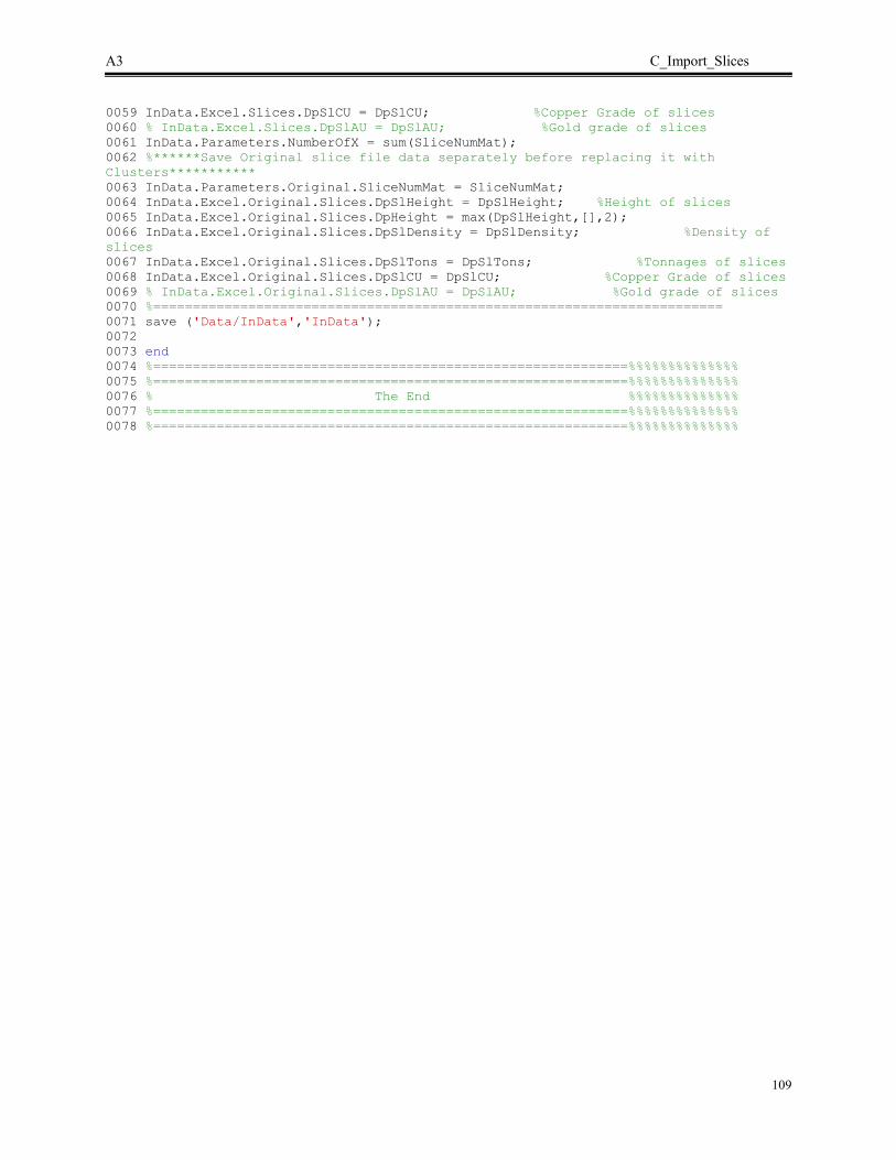
A3 C_Import_Slices
109
0059 InData.Excel.Slices.DpSlCU = DpSlCU; %Copper Grade of slices
0060 % InData.Excel.Slices.DpSlAU = DpSlAU; %Gold grade of slices
0061 InData.Parameters.NumberOfX = sum(SliceNumMat);
0062 %******Save Original slice file data separately before replacing it with
Clusters***********
0063 InData.Parameters.Original.SliceNumMat = SliceNumMat;
0064 InData.Excel.Original.Slices.DpSlHeight = DpSlHeight; %Height of slices
0065 InData.Excel.Original.Slices.DpHeight = max(DpSlHeight,[],2);
0066 InData.Excel.Original.Slices.DpSlDensity = DpSlDensity; %Density of
slices
0067 InData.Excel.Original.Slices.DpSlTons = DpSlTons; %Tonnages of slices
0068 InData.Excel.Original.Slices.DpSlCU = DpSlCU; %Copper Grade of slices
0069 % InData.Excel.Original.Slices.DpSlAU = DpSlAU; %Gold grade of slices
0070 %========================================================================
0071 save ('Data/InData','InData');
0072
0073 end
0074 %============================================================%%%%%%%%%%%%%%
0075 %============================================================%%%%%%%%%%%%%%
0076 % The End %%%%%%%%%%%%%%
0077 %============================================================%%%%%%%%%%%%%%
0078 %============================================================%%%%%%%%%%%%%%

110
A4. E_ScenarioGenerator_HVConeMixing
0001 %============================================================%%%%%%%%%%%%%%
0002 %============================================================%%%%%%%%%%%%%%
0003 % University of Alberta %%%%%%%%%%%%%%
0004 % Department of Civil and Environmental Engineering %%%%%%%%%%%%%%
0005 % School of Mining and Petroleum Engineering %%%%%%%%%%%%%%
0006 % This program was written by: Firouz Khodayari, %%%%%%%%%%%%%%
0007 % Student ID: 1402853 %%%%%%%%%%%%%%
0008 % PhD Candidate in Mining Engineering %%%%%%%%%%%%%%
0009 %============================================================%%%%%%%%%%%%%%
0010 %============================================================%%%%%%%%%%%%%%
0011
0012 function E_ScenarioGenerator_HVConeMixing
0013
0014 %This function generates both grade and tonnage scenarios by sampling form
0015 %grade and tonnage original data from drawpoints and their adjacent ones
0016 %which means both vertical and horizontal dilutions (movements) are
0017 %considered at the same time
0018 %========================================
0019 load('Data/Param.mat'); %Loading the input parameters
0020 load('Data/InData.mat');
0021 if exist('Data/ModelF.mat')== 2
0022 load('Data/ModelF.mat');
0023
0024 else
0025 end
0026 T = Param.T; %number of periods
0027 N = InData.Parameters.N; %number of drawpoints(draw columns)
0028 X_DPs = InData.Excel.DPs.X;
0029 Y_DPs = InData.Excel.DPs.Y;
0030 AdjRadius = Param.AdjRadius;
0031 NumberOfX = InData.Parameters.NumberOfX;
0032 ScenNum = Param.ScenNum;
0033 SliceNumMat = InData.Parameters.SliceNumMat; %the Matrix which shows how many
slices are in each drawcolumn
0034 Ton = InData.Excel.Slices.DpSlTons; %Height of Clusters
0035 Density = InData.Excel.Slices.DpSlDensity; %Tonnages of Clusters
0036 Grade = InData.Excel.Slices.DpSlCU; %Copper Grade of Clusters
0037 DpSlHeight = InData.Excel.Slices.DpSlHeight;
0038 HD = Param.HD; %Mixing Parameter ********************
0039 VSA = Param.VSA; %Mixing Parameter ********************
0040 X_DPs_Vvector = InData.Excel.DPs.X;
0041 Y_DPs_Vvector = InData.Excel.DPs.Y;
0042
0043 X_DPs_Hvector = X_DPs_Vvector';
0044 Y_DPs_Hvector = Y_DPs_Vvector';
0045 %*****************************************************
0046
0047 %#########################################################################
0048 %Distance Calculator (finding teh adjacent drawpoints for each drawpoint)
0049 %#########################################################################
0050
0051 %========================================= calculating distance between
drawpoints in X direction, Craete dX^2
0052 X_DPS_1 = repmat(X_DPs_Hvector,N,1);
0053 X_DPS_2 = repmat(X_DPs_Vvector,1,N);
0054
0055 dX = (X_DPS_1)-(X_DPS_2);
0056 dX_square = dX.^2;
0057

A4 E_ScenarioGenerator_HVConeMixing
111
0058 %========================================= calculating distance between
drawpoints in Y direction, Craete dY^2
0059 Y_DPS_1 = repmat(Y_DPs_Hvector,N,1);
0060 Y_DPS_2 = repmat(Y_DPs_Vvector,1,N);
0061
0062 dY = (Y_DPS_1)-(Y_DPS_2);
0063 dY_square = dY.^2;
0064
0065 %========================================= DISTANCE^2=dX^2+dY^2
0066 Distance_square = dX_square+dY_square;
0067
0068 %========================================= Distance between darwpoints
0069 Distance_DPs = sqrt(Distance_square);
0070 %#########################################################################
0071 Adjacents = [];
0072 Adjacents = cell(N,1);
0073 for iloop = 1:N
0074 temp = find(Distance_DPs(iloop,:)<=AdjRadius & Distance_DPs(iloop,:)>0);
0075 %indices(i,1:numel(temp)) = temp;
0076 temp = [iloop,temp];
0077 Adjacents{iloop,1} = temp;
0078 end
0079 %Tonnage and Grade*********************************************************
0080 SlcCnt = 0;
0081 TempMat0 = zeros(1,T*NumberOfX);
0082 SumTempGrade = zeros(size(Grade,1),size(Grade,2));
0083 SumTempTon = zeros(size(Ton,1),size(Ton,2));
0084 for dp = 1:N
0085 DpAdj = Adjacents{dp,1};
0086 for Slc = 1:SliceNumMat(dp,1);
0087 cx = X_DPs(dp,1);
0088 cy = Y_DPs(dp,1);
0089 cz = DpSlHeight(dp,Slc)-(DpSlHeight(dp,1)/2);
0090 r0 = 0;
0091 rh = HD;
0092 h = rh/tand(VSA);
0093 SlcCnt = SlcCnt + 1;
0094 SlcAdjCnt = 0;
0095 %===============================
0096 for AdjCount = 1:numel(DpAdj)
0097 Adjtemp = DpAdj(1, AdjCount);
0098 for SlcAdj = 1:SliceNumMat(Adjtemp,1);
0099 px = X_DPs(Adjtemp,1);
0100 py = Y_DPs(Adjtemp,1);
0101 pz = DpSlHeight(Adjtemp,SlcAdj)-(DpSlHeight(Adjtemp,1)/2);
0102 if (h^2)*((px-cx)^2)+(h^2)*((py-cy)^2) <= ((h-pz)*r0+pz*rh)^2
&& pz <= cz + h
0103 SlcAdjCnt = SlcAdjCnt + 1;
0104 DataGrade(SlcCnt,SlcAdjCnt) = Grade(Adjtemp,SlcAdj);
0105 DataDensity(SlcCnt,SlcAdjCnt) = Density(Adjtemp,SlcAdj);
0106 else
0107 %Nothing
0108 end
0109 end
0110 end
0111 TempGrade = datasample(DataGrade(SlcCnt,1:SlcAdjCnt),ScenNum);
0112 TempDensity =
datasample(DataDensity(SlcCnt,1:SlcAdjCnt),ScenNum);
0113 for jloop = 1:ScenNum
0114 eval(sprintf('Scenarios.Grade.GradeScen%d(dp,Slc) =
TempGrade(jloop)',jloop));
0115 eval(sprintf('Scenarios.Ton.TonScen%d(dp,Slc) =
TempDensity(jloop)*((Ton(dp,Slc))/(Density(dp,Slc)))',jloop));

A4 E_ScenarioGenerator_HVConeMixing
112
0116 SumTempGrade(dp,Slc) = SumTempGrade(dp,Slc) +
TempGrade(jloop);
0117 SumTempTon(dp,Slc) = SumTempTon(dp,Slc) +
(TempDensity(jloop)*((Ton(dp,Slc))/(Density(dp,Slc))));
0118 end
0119 end
0120 end
0121
0122 EGrade = SumTempGrade./ScenNum;
0123 ETon = SumTempTon./ScenNum;
0124 GradeVarMat = zeros(1,NumberOfX);
0125 EGradeVarMat = zeros(1,NumberOfX);
0126 TonVarMat = zeros(1,NumberOfX);
0127 ETonVarMat = zeros(1,NumberOfX);
0128 VarCount1 = 0;
0129 VarCount2 = 0;
0130 for tloop = 1:T
0131
0132 for iloop = 1:N
0133 VarCount2 = VarCount2 + SliceNumMat(iloop,1);
0134 if tloop ==1
0135 TonVarMat(1,VarCount1+1:VarCount2) =
Ton(iloop,1:SliceNumMat(iloop,1));
0136 GradeVarMat(1,VarCount1+1:VarCount2) =
Grade(iloop,1:SliceNumMat(iloop,1));
0137 EGradeVarMat(1,VarCount1+1:VarCount2) =
EGrade(iloop,1:SliceNumMat(iloop,1));
0138 ETonVarMat(1,VarCount1+1:VarCount2) =
ETon(iloop,1:SliceNumMat(iloop,1));
0139 for jloop = 1:ScenNum
0140 TempMatGrade2 =
Scenarios.Grade.(['GradeScen',num2str(jloop)])(iloop,1:SliceNumMat(iloop,1));
0141
eval(sprintf('Scenarios.Grade.GradeScenVarMat%d(1,VarCount1+1:VarCount2) =
TempMatGrade2',jloop));
0142 TempMatTon2 =
Scenarios.Ton.(['TonScen',num2str(jloop)])(iloop,1:SliceNumMat(iloop,1));
0143
eval(sprintf('Scenarios.Ton.TonScenVarMat%d(1,VarCount1+1:VarCount2) =
TempMatTon2',jloop));
0144 end
0145 else
0146 end
0147 VarCount1 = VarCount1 + SliceNumMat(iloop,1);
0148
0149 end
0150 end
0151 ModelF.Inputs.TonVarMat = TonVarMat;
0152 ModelF.Inputs.GradeVarMat = GradeVarMat;
0153 ModelF.Inputs.Scenarios.Grade.EGradeVarMat = EGradeVarMat;
0154 ModelF.Inputs.Scenarios.Ton.ETonVarMat = ETonVarMat;
0155 ModelF.Inputs.Scenarios.Grade.Scen = Scenarios.Grade;
0156 ModelF.Inputs.Scenarios.Grade.EGrade = EGrade;
0157 ModelF.Inputs.Scenarios.Ton.Scen = Scenarios.Ton;
0158 ModelF.Inputs.Scenarios.Ton.ETon = ETon;
0159 ModelF.Inputs.Scenarios.ScenNum = ScenNum;
0160 ModelF.Inputs.Adjacents = Adjacents;
0161 save ('Data/InData','InData');
0162 save('Data/ModelF','ModelF');
0163 end
0164 %============================================================%%%%%%%%%%%%%%
0165 %============================================================%%%%%%%%%%%%%%
0166 % The End %%%%%%%%%%%%%%

A4 E_ScenarioGenerator_HVConeMixing
113
0167 %============================================================%%%%%%%%%%%%%%
0168 %============================================================%%%%%%%%%%%%%%

114
A5. F_MiningDirectionEvaluation
0001 %============================================================%%%%%%%%%%%%%%
0002 %============================================================%%%%%%%%%%%%%%
0003 % University of Alberta %%%%%%%%%%%%%%
0004 % Department of Civil and Environmental Engineering %%%%%%%%%%%%%%
0005 % School of Mining and Petroleum Engineering %%%%%%%%%%%%%%
0006 % This program was written by: Firouz Khodayari, %%%%%%%%%%%%%%
0007 % Student ID: 1402853 %%%%%%%%%%%%%%
0008 % PhD Candidate in Mining Engineering %%%%%%%%%%%%%%
0009 %============================================================%%%%%%%%%%%%%%
0010 %============================================================%%%%%%%%%%%%%%
0011
0012 function F_MiningDirectionEvaluation
0013
0014 load('Data/Param.mat');
0015 load('Data/InData.mat');
0016 if exist('Data/ModelF.mat')== 2
0017 load('Data/ModelF.mat');
0018 else
0019 end
0020 T = Param.T;
0021 N = InData.Parameters.N;
0022 Adjacents = ModelF.Inputs.Adjacents;
0023 DEV = InData.Excel.DPs.DEV;
0024
0025 PB = zeros(N,1);
0026 for i = 1:N
0027
0028 PB(i,1) = sum(DEV(Adjacents{i,1}))+DEV(i,1);
0029
0030 end
0031
0032 InData.PB = PB;
0033 save('Data/ModelF','ModelF');
0034 save('Data/InData','InData');
0035 Plot_PB_DEV
0036 end
0037 %============================================================%%%%%%%%%%%%%%
0038 %============================================================%%%%%%%%%%%%%%
0039 % The End %%%%%%%%%%%%%%
0040 %============================================================%%%%%%%%%%%%%%
0041 %============================================================%%%%%%%%%%%%%%

115
A6. ObjectiveFunction_MILP_Stoch
0001 %============================================================%%%%%%%%%%%%%%
0002 %============================================================%%%%%%%%%%%%%%
0003 % University of Alberta %%%%%%%%%%%%%%
0004 % Department of Civil and Environmental Engineering %%%%%%%%%%%%%%
0005 % School of Mining and Petroleum Engineering %%%%%%%%%%%%%%
0006 % This program was written by: Firouz Khodayari, %%%%%%%%%%%%%%
0007 % Student ID: 1402853 %%%%%%%%%%%%%%
0008 % PhD Candidate in Mining Engineering %%%%%%%%%%%%%%
0009 %============================================================%%%%%%%%%%%%%%
0010 %============================================================%%%%%%%%%%%%%%
0011
0012 function ObjectiveFunction_MILP_Stoch
0013
0014 %This function is used to create the coefficient matrix of the objective
0015 %function and save it in the MATLAB structure
0016 %#########################################################
0017 % Minimize sum(sum(Absolute(tonij-ton0ij))) ===> Minimize sum(sum(Zij))
0018 % ModelF format: fval = C'*x #
0019 %#########################################################
0020 load('Data/Param.mat');
0021 load('Data/InData.mat');
0022 if exist('Data/ModelF.mat')== 2
0023 load('Data/ModelF.mat');
0024 else
0025 end
0026
0027 T = Param.T;
0028 N = InData.Parameters.N;
0029 ScenariosTon = ModelF.Inputs.Scenarios.Ton;
0030 ScenariosGrade = ModelF.Inputs.Scenarios.Grade;
0031 price = Param.price;
0032 ton = InData.Excel.Slices.DpSlTons;
0033 grade = InData.Excel.Slices.DpSlCU;
0034 rec = Param.recovery;
0035 cost = Param.cost;
0036 r = Param.Intrate;
0037 SliceNumMat = InData.Parameters.SliceNumMat;
0038 NumberOfX = InData.Parameters.NumberOfX;
0039 %Parameters
0040 MiningCapacity_st = Param.Mst*1000000; %Starting production rate or mining
capacity (based on production Curve)
0041 MiningCapacity_max = Param.Mmax*1000000; %Maximum production rate or mining
capacity
0042 RampUpTime = Param.RampUpTime; %Ramp Up time for the production schedule
0043 ScenNum = Param.ScenNum;
0044 GradeDevCost = Param.GradeDevCost;
0045 TonDevCost = Param.TonDevCost;
0046 TarGrade = Param.TarGrade;
0047 MiningCapacity_st = Param.Mst*1000000; %Starting production rate or mining
capacity (based on production Curve)
0048 MiningCapacity_max = Param.Mmax*1000000; %Maximum production rate or mining
capacity
0049 RampUpTime = Param.RampUpTime; %Ramp Up time for the production schedule
0050 %@@@@@@@@@@@
0051 TonVarMat = ModelF.Inputs.TonVarMat;
0052 GradeVarMat = ModelF.Inputs.GradeVarMat;
0053 EGradeVarMat = ModelF.Inputs.Scenarios.Grade.EGradeVarMat;
0054 ETonVarMat = ModelF.Inputs.Scenarios.Ton.ETonVarMat;
0055 ETon = ModelF.Inputs.Scenarios.Ton.ETon;
0056 EGrade = ModelF.Inputs.Scenarios.Grade.EGrade;
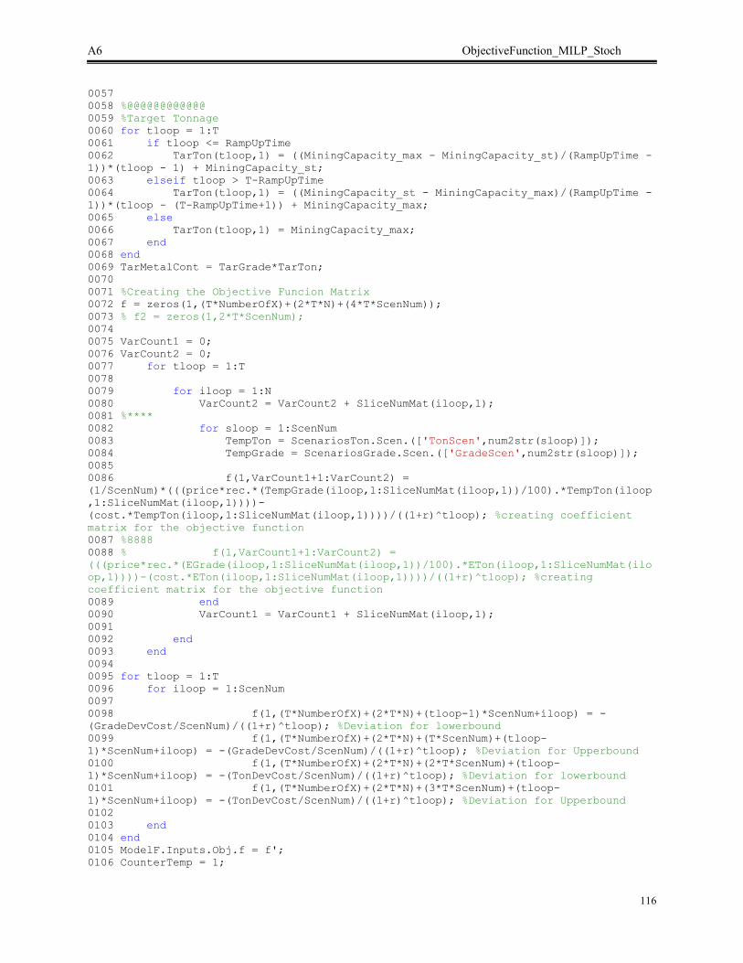
A6 ObjectiveFunction_MILP_Stoch
116
0057
0058 %@@@@@@@@@@@@
0059 %Target Tonnage
0060 for tloop = 1:T
0061 if tloop <= RampUpTime
0062 TarTon(tloop,1) = ((MiningCapacity_max - MiningCapacity_st)/(RampUpTime -
1))*(tloop - 1) + MiningCapacity_st;
0063 elseif tloop > T-RampUpTime
0064 TarTon(tloop,1) = ((MiningCapacity_st - MiningCapacity_max)/(RampUpTime -
1))*(tloop - (T-RampUpTime+1)) + MiningCapacity_max;
0065 else
0066 TarTon(tloop,1) = MiningCapacity_max;
0067 end
0068 end
0069 TarMetalCont = TarGrade*TarTon;
0070
0071 %Creating the Objective Funcion Matrix
0072 f = zeros(1,(T*NumberOfX)+(2*T*N)+(4*T*ScenNum));
0073 % f2 = zeros(1,2*T*ScenNum);
0074
0075 VarCount1 = 0;
0076 VarCount2 = 0;
0077 for tloop = 1:T
0078
0079 for iloop = 1:N
0080 VarCount2 = VarCount2 + SliceNumMat(iloop,1);
0081 %****
0082 for sloop = 1:ScenNum
0083 TempTon = ScenariosTon.Scen.(['TonScen',num2str(sloop)]);
0084 TempGrade = ScenariosGrade.Scen.(['GradeScen',num2str(sloop)]);
0085
0086 f(1,VarCount1+1:VarCount2) =
(1/ScenNum)*(((price*rec.*(TempGrade(iloop,1:SliceNumMat(iloop,1))/100).*TempTon(iloop
,1:SliceNumMat(iloop,1))))-
(cost.*TempTon(iloop,1:SliceNumMat(iloop,1))))/((1+r)^tloop); %creating coefficient
matrix for the objective function
0087 %8888
0088 % f(1,VarCount1+1:VarCount2) =
(((price*rec.*(EGrade(iloop,1:SliceNumMat(iloop,1))/100).*ETon(iloop,1:SliceNumMat(ilo
op,1))))-(cost.*ETon(iloop,1:SliceNumMat(iloop,1))))/((1+r)^tloop); %creating
coefficient matrix for the objective function
0089 end
0090 VarCount1 = VarCount1 + SliceNumMat(iloop,1);
0091
0092 end
0093 end
0094
0095 for tloop = 1:T
0096 for iloop = 1:ScenNum
0097
0098 f(1,(T*NumberOfX)+(2*T*N)+(tloop-1)*ScenNum+iloop) = -
(GradeDevCost/ScenNum)/((1+r)^tloop); %Deviation for lowerbound
0099 f(1,(T*NumberOfX)+(2*T*N)+(T*ScenNum)+(tloop-
1)*ScenNum+iloop) = -(GradeDevCost/ScenNum)/((1+r)^tloop); %Deviation for Upperbound
0100 f(1,(T*NumberOfX)+(2*T*N)+(2*T*ScenNum)+(tloop-
1)*ScenNum+iloop) = -(TonDevCost/ScenNum)/((1+r)^tloop); %Deviation for lowerbound
0101 f(1,(T*NumberOfX)+(2*T*N)+(3*T*ScenNum)+(tloop-
1)*ScenNum+iloop) = -(TonDevCost/ScenNum)/((1+r)^tloop); %Deviation for Upperbound
0102
0103 end
0104 end
0105 ModelF.Inputs.Obj.f = f';
0106 CounterTemp = 1;

A6 ObjectiveFunction_MILP_Stoch
117
0107 DrawID = zeros(N,1);
0108 for iloop = 1:N
0109 DrawID(iloop,1) = CounterTemp;
0110 CounterTemp = CounterTemp + SliceNumMat(iloop,1);
0111 end
0112 ModelF.Inputs.DrawID = DrawID;
0113 ModelF.Inputs.TarMetalCont = TarMetalCont;
0114 InData.Parameters.NumberOfX = NumberOfX;
0115 save('Data/ModelF','ModelF');
0116 save('Data/InData','InData');
0117
0118 end
0119 %============================================================%%%%%%%%%%%%%%
0120 %============================================================%%%%%%%%%%%%%%
0121 % The End %%%%%%%%%%%%%%
0122 %============================================================%%%%%%%%%%%%%%
0123 %============================================================%%%%%%%%%%%%%%

118
A7. Const_ActiveDrawpoints
0001 %============================================================%%%%%%%%%%%%%%
0002 %============================================================%%%%%%%%%%%%%%
0003 % University of Alberta %%%%%%%%%%%%%%
0004 % Department of Civil and Environmental Engineering %%%%%%%%%%%%%%
0005 % School of Mining and Petroleum Engineering %%%%%%%%%%%%%%
0006 % This program was written by: Firouz Khodayari, %%%%%%%%%%%%%%
0007 % Student ID: 1402853 %%%%%%%%%%%%%%
0008 % PhD Candidate in Mining Engineering %%%%%%%%%%%%%%
0009 %============================================================%%%%%%%%%%%%%%
0010 %============================================================%%%%%%%%%%%%%%
0011
0012 function Const_ActiveDrawpoints
0013 %This function creates the coefficient matrices for number of active
0014 %drawpoints in order to control the number of operating drawpoints for each
0015 %period
0016
0017 %############################################################
0018 % Number of Active Drawpoints #
0019 %############################################################
0020 %***********************************************************************
0021 % for each t =======> ActMin <= sum(Y1) <= ActMax
0022 %***********************************************************************
0023 load('Data/Param.mat'); %Loading the input parameters
0024 load('Data/InData.mat');
0025 if exist('Data/ModelF.mat')== 2
0026 load('Data/ModelF.mat');
0027 else
0028 end
0029
0030 T = Param.T; %number of periods
0031 N = InData.Parameters.N; %number of drawpoints(draw columns)
0032 NumberOfX = InData.Parameters.NumberOfX;
0033 DrawID = ModelF.Inputs.DrawID;
0034 ScenNum = Param.ScenNum;
0035
0036 %**********************%****
0037 %***********************%***
0038 NoOfActiveDP_min = Param.Actmin; %Minimum number of active drawpoints per
period
0039 NoOfActiveDP_max = Param.Actmax; %Maximum number of active drawpoints per
period
0040 %**********************%****
0041 %*********************%*****
0042 ModelF.Inputs.Parameters.NoOfActiveDP_min = NoOfActiveDP_min;
0043 ModelF.Inputs.Parameters.NoOfActiveDP_max = NoOfActiveDP_max;
0044 %*********************%*****
0045 DpActVar = sparse(T,T*N);
0046 for tloop = 1:T;
0047 DpActVar(tloop,(tloop-1)*N+1:tloop*N) = 1;
0048 end
0049 % aa = full(DpActVar);
0050 ModelF.Inputs.Constraints.Parameters.DpActVar = DpActVar; %Drawpoint Activation
Variable per period, if a drawpoint has extraction using it's column, then it is
active
0051
0052 Aeq_p1 = sparse(T,T*NumberOfX);
0053 Aeq_p2 = DpActVar;
0054 Aeq_p3 = sparse(T,T*N);
0055 Aeq_p4 = sparse(T,4*T*ScenNum);
0056
A7 Const_ActiveDrawpoints
119
0057 Aineq_ActiveDrawPoints = [Aeq_p1,Aeq_p2,Aeq_p3,Aeq_p4]; %Left hand side, the
maximum number of active drawpints per each period of t
0058 bineq_ActiveDrawPoints_U = NoOfActiveDP_max * ones(T,1); % right hand sidethe
maximum number of active drawpints per each period of t
0059 bineq_ActiveDrawPoints_L = NoOfActiveDP_min * ones(T,1); % right hand sidethe
maximum number of active drawpints per each period of t
0060
0061 ModelF.Inputs.Constraints.Aineq_ActiveDrawPoints = Aineq_ActiveDrawPoints; % the
left hand side matrix for the Number of Active Drawpoints constrain
0062 save('Data/ModelF','ModelF');
0063
0064 ModelF.Inputs.Constraints.bineq_ActiveDrawPoints_U = bineq_ActiveDrawPoints_U; %
the Right hand side matrix for the Number of Active Drawpoints
0065 ModelF.Inputs.Constraints.bineq_ActiveDrawPoints_L = bineq_ActiveDrawPoints_L; %
the Left hand side matrix for the Number of Active Drawpoints
0066
0067 save('Data/ModelF','ModelF');
0068
0069 end
0070 %============================================================%%%%%%%%%%%%%%
0071 %============================================================%%%%%%%%%%%%%%
0072 % The End %%%%%%%%%%%%%%
0073 %============================================================%%%%%%%%%%%%%%
74 %============================================================%%%%%%%%%%%%%%

120
A8. Const_Binary_Slc
0001 %============================================================%%%%%%%%%%%%%%
0002 %============================================================%%%%%%%%%%%%%%
0003 % University of Alberta %%%%%%%%%%%%%%
0004 % Department of Civil and Environmental Engineering %%%%%%%%%%%%%%
0005 % School of Mining and Petroleum Engineering %%%%%%%%%%%%%%
0006 % This program was written by: Firouz Khodayari, %%%%%%%%%%%%%%
0007 % Student ID: 1402853 %%%%%%%%%%%%%%
0008 % PhD Candidate in Mining Engineering %%%%%%%%%%%%%%
0009 %============================================================%%%%%%%%%%%%%%
0010 %============================================================%%%%%%%%%%%%%%
0011
0012 function Const_Binary_Slc
0013 %This function creates the coefficient matrices for the binary variables in the
model
0014 % 4 set of binary variables are defined in order to be able to define the
0015 % related constraints for the Mixed Integer Quadratic Programming (MIQP)
0016 % Model:
0017
0018 %{Y1} Set 1: variables (T*NumberOfX)+1 to (2*T*NumberOfX)
0019 %this set determines if the slice i is active in period t or not so
0020 %that if there is extraction in that (x>0) then Y1=1 and if
0021 %there is no extraction (x=0) then Y1=0
0022 %{Y2} Set 2: Variables (2*T*NumberOfX)+1 to 3*T*NumberOfX
0023 %this set determines if the drawpoint i is active in period t or not so
0024 %that if there is extraction in that (x>0) then Y2=1 and if
0025 %there is no extraction (x=0) then Y2=0
0026 %{Y3} Set 3: Variables (3*T*NumberOfX)+1 to 4*T*NumberOfX
0027 %this set determines if drawpoint i has started its production or not. In
other words the depletion percentage of drawpoint i in period t is 0 or not
0028 %if the depletion percentage is 0 (DP=0) then Y3=0 and if depletion
0029 %percentage is greater than 0 (DP>0) then Y3=1
0030 %depletion percentage (DP) is the summation of the x values for drawpoint i
from
0031 %period 1 till period t
0032
%*************************************************************************************
********************************
0033 load('Data/Param.mat'); %Loading the input parameters
0034 load('Data/InData.mat');
0035 if exist('Data/ModelF.mat')== 2
0036 load('Data/ModelF.mat');
0037 else
0038 end
0039
0040 T = Param.T; %number of periods
0041 N = InData.Parameters.N; %number of drawpoints(draw columns)
0042 NumberOfX = InData.Parameters.NumberOfX;
0043 SliceNumMat = InData.Parameters.SliceNumMat; %the Matrix which shows how many
slices are in each drawcolumn
0044 DrawID = ModelF.Inputs.DrawID;
0045 ScenNum = Param.ScenNum;
0046
0047 %*****************************************************
0048 %Parameters
0049 M = Param.M; %an arbitrary big number
0050
0051 % %############################################################
0052 % % Set 1 ===> Active Slices (Sls) #
0053 % %############################################################
0054 % %***************************************

A8 Const_Binary_Slc
121
0055 % % eq1 =======> y1-M1x <=0
0056 % % eq2 =======> x-M*y1<=0
0057 % %***************************************
0058 % %Left hand sides
0059 % Aeq_S1_eq1_p1 = (-M)*speye(T*NumberOfX); % -M*x
0060 % Aeq_S1_eq1_p2 = speye(T*NumberOfX); % y1
0061 % Aeq_S1_eq1_p3 = sparse(T*NumberOfX,T*NumberOfX);
0062 % Aeq_S1_eq1_p4 = sparse(T*NumberOfX,T*NumberOfX);
0063 % Aeq_S1_eq1_p5 = sparse(T*NumberOfX,2*T*ScenNum);
0064 %
0065 % Aeq_S1_eq2_p1 = speye(T*NumberOfX); % x
0066 % Aeq_S1_eq2_p2 = (-M)*speye(T*NumberOfX); % -M*y1
0067 % Aeq_S1_eq2_p3 = sparse(T*NumberOfX,T*NumberOfX);
0068 % Aeq_S1_eq2_p4 = sparse(T*NumberOfX,T*NumberOfX);
0069 % Aeq_S1_eq2_p5 = sparse(T*NumberOfX,2*T*ScenNum);
0070 %
0071 % %concatination
0072 % Aeq_S1_eq1 =
[Aeq_S1_eq1_p1,Aeq_S1_eq1_p2,Aeq_S1_eq1_p3,Aeq_S1_eq1_p4,Aeq_S1_eq1_p5]; % y1-Mx <=0
0073 % Aeq_S1_eq2 =
[Aeq_S1_eq2_p1,Aeq_S1_eq2_p2,Aeq_S1_eq2_p3,Aeq_S1_eq2_p4,Aeq_S1_eq2_p5]; % x-y1 <=0
0074 %
0075 % %Right hand sides
0076 % beq_S1_eq1 = sparse(T*NumberOfX,1); %right hand side matrix for the first
equation y1-Mx <=0
0077 % beq_S1_eq2 = sparse(T*NumberOfX,1); %right hand side matrix for the second
equation x-y1 <=0
0078
0079 %############################################################
0080 % Set 2 ===> Active DrawPoints (DPs) #
0081 %############################################################
0082 %***************************************
0083 % eq1 =======> y2-Mx <=0
0084 % eq2 =======> x-M*y2<=0
0085 %***************************************
0086 %############################################################
0087 % PRECALCULATIONS for the rest of the binary variables
0088 %############################################################
0089 %Defining the required matrix to calculate the Depletion Percentage for each
0090 %drawpoint at each periodDDP = sparse(T*N,T*NumberOfX); %DP = sum(x) , for t <=
ti
0091 Y3MAT = sparse(T*N,T*NumberOfX);
0092 VarCount1 = 0;
0093 VarCount2 = 0;
0094 Y2MATTemp = sparse(N,NumberOfX);
0095 DDPtemp = sparse(N,NumberOfX);
0096 for iloop = 1:N;
0097 VarCount2 = VarCount2 + SliceNumMat(iloop,1);
0098 DDPtemp(iloop,VarCount1+1:VarCount2) = 1;
0099 Y2MATTemp(iloop,VarCount1+1) = 1;
0100 VarCount1 = VarCount1 + SliceNumMat(iloop,1);
0101 end
0102 DpActTemp = eye(N);
0103 bb = eye(T);
0104 DpAct = kron(bb,DpActTemp);
0105 Y2MAT = kron(bb,Y2MATTemp);
0106 XMAT = kron(bb,DDPtemp);
0107 DDP = sparse(T*N,T*N);
0108 for tloop = 1:T
0109 a = sparse(tloop:T,1:T-tloop+1,1,T,T);
0110 dptloop = kron(a,DpActTemp);
0111 DDP = DDP + dptloop;
0112 end

A8 Const_Binary_Slc
122
0113 cc = eye(T);
0114 DpStart = kron(cc,DpActTemp);
0115 Y3MAT = kron(cc,Y2MATTemp);
0116 %*****
0117 %Left hand sides
0118 Aeq_S2_eq1_p1 = -M*XMAT; % -M1*x
0119 Aeq_S2_eq1_p2 = DpAct; % y2
0120 Aeq_S2_eq1_p3 = sparse(T*N,T*N);
0121 Aeq_S2_eq1_p4 = sparse(T*N,4*T*ScenNum);
0122
0123 Aeq_S2_eq2_p1 = XMAT; % x
0124 Aeq_S2_eq2_p2 = (-M)*DpAct; % -M*y2
0125 Aeq_S2_eq2_p3 = sparse(T*N,T*N);
0126 Aeq_S2_eq2_p4 = sparse(T*N,4*T*ScenNum);
0127
0128 %concatination
0129 Aeq_S2_eq1 = [Aeq_S2_eq1_p1,Aeq_S2_eq1_p2,Aeq_S2_eq1_p3,Aeq_S2_eq1_p4]; % y1-Mx
<=0
0130 Aeq_S2_eq2 = [Aeq_S2_eq2_p1,Aeq_S2_eq2_p2,Aeq_S2_eq2_p3,Aeq_S2_eq2_p4]; % x-y1
<=0
0131
0132 %Right hand sides
0133 beq_S2_eq1 = sparse(T*N,1); %right hand side matrix for the first equation y1-Mx
<=0
0134 beq_S2_eq2 = sparse(T*N,1); %right hand side matrix for the second equation x-y1
<=0
0135
0136 % %############################################################
0137 % Set 3 ===> Has the DP been opened? #
0138 % %############################################################
0139 % %***************************************
0140 % % DDP <= y =====> DDP - M*y3 <= 0
0141 % % y <= M*DDP =====> y3 - M*DDP <= 0
0142 % %***************************************
0143
0144 Aeq_S3_eq1_p1 = sparse(T*N,T*NumberOfX); %DPP This has to be only for drawpoints
not for columns, because we will be using that for the precedence constraint!
0145 Aeq_S3_eq1_p2 = DDP;
0146 Aeq_S3_eq1_p3 = -M*DpStart; % -y3
0147 Aeq_S3_eq1_p4 = sparse(T*N,4*T*ScenNum);
0148
0149
0150 Aeq_S3_eq2_p1 = sparse(T*N,T*NumberOfX);
0151 Aeq_S3_eq2_p2 = -M*DDP; % -(M*DDP)
0152 Aeq_S3_eq2_p3 = DpStart; % y3
0153 Aeq_S3_eq2_p4 = sparse(T*N,4*T*ScenNum);
0154
0155
0156 beq_S3_eq1 = sparse(T*N,1); %right hand side matrix for the first equation "DP -
y <=0"
0157 beq_S3_eq2 = sparse(T*N,1); %right hand side matrix for the second equation "y -
M*DP <= 0"
0158
0159 %concatination
0160 Aeq_S3_eq1 = [Aeq_S3_eq1_p1,Aeq_S3_eq1_p2,Aeq_S3_eq1_p3,Aeq_S3_eq1_p4]; % DP - y
<= DCF
0161 Aeq_S3_eq2 = [Aeq_S3_eq2_p1,Aeq_S3_eq2_p2,Aeq_S3_eq2_p3,Aeq_S3_eq2_p4]; % y - DP
<= (1-DCF)
0162
0163
%#####################################################################################
#########################
0164 %Concatinating the matrices

A8 Const_Binary_Slc
123
0165
%#####################################################################################
#########################
0166
0167 %creating the last matrix which is the concatenation of all constraints
0168 %related to the binary variables for 0 and 1 situations
0169
0170 Aineq_Binary = [Aeq_S2_eq1;Aeq_S2_eq2;Aeq_S3_eq1;Aeq_S3_eq2];
0171 bineq_Binary_U = [beq_S2_eq1;beq_S2_eq2;beq_S3_eq1;beq_S3_eq2];
0172 SizeTemp = size(bineq_Binary_U,1);
0173 bineq_Binary_L = -inf*ones(SizeTemp,1);
0174 ModelF.Inputs.Constraints.Aineq_Binary = Aineq_Binary;
0175 ModelF.Inputs.Constraints.bineq_Binary_U = bineq_Binary_U;
0176 ModelF.Inputs.Constraints.bineq_Binary_L = bineq_Binary_L;
0177
0178 %Saving
0179 save('Data/ModelF','ModelF');
0180 end
0181 %============================================================%%%%%%%%%%%%%%
0182 %============================================================%%%%%%%%%%%%%%
0183 % The End %%%%%%%%%%%%%%
0184 %============================================================%%%%%%%%%%%%%%
0185 %============================================================%%%%%%%%%%%%%%

124
A9. Const_ContinuousMining
0001 %============================================================%%%%%%%%%%%%%%
0002 %============================================================%%%%%%%%%%%%%%
0003 % University of Alberta %%%%%%%%%%%%%%
0004 % Department of Civil and Environmental Engineering %%%%%%%%%%%%%%
0005 % School of Mining and Petroleum Engineering %%%%%%%%%%%%%%
0006 % This program was written by: Firouz Khodayari, %%%%%%%%%%%%%%
0007 % Student ID: 1402853 %%%%%%%%%%%%%%
0008 % PhD Candidate in Mining Engineering %%%%%%%%%%%%%%
0009 %============================================================%%%%%%%%%%%%%%
0010 %============================================================%%%%%%%%%%%%%%
0011
0012 function Const_ContinuousMining
0013
0014 %This function is going to control the continuous mining operation for drawpoints
0015 %*******************
0016 %loading the matlab file (InData.mat) which contains the input data that we are
going to use for defining this constraint
0017 %loading the matlab file (ModelF.mat) if it exists to save the built matrixin
that.
0018 %depends on the order in which we run the constraints and objective function
functionsthis file may exist or not, so we use if function
0019 load('Data/Param.mat'); %Loading the input parameters
0020 load('Data/InData.mat');
0021 if exist('Data/ModelF.mat')== 2
0022 load('Data/ModelF.mat');
0023 else
0024 end
0025
0026 %Calling the related inputs
0027 T = Param.T; %number of periods
0028 N = InData.Parameters.N; %number of drawpoints(draw columns)
0029 NumberOfX = InData.Parameters.NumberOfX;
0030 DrawID = ModelF.Inputs.DrawID;
0031 ScenNum = Param.ScenNum;
0032
0033 %****************************************************
0034
0035 ContinMin1 = sparse((T-1)*N,T*N);
0036 ContinMin2 = sparse((T-1)*N,T*N);
0037
0038 for tloop = 1:T-1
0039 for iloop = 1:N
0040 ContinMin1((tloop-1)*N+iloop,(tloop-1)*N+iloop) = -1; %One period before
0041 ContinMin1((tloop-1)*N+iloop,(tloop-1)*N+N+iloop) = 1; %Same period
0042 ContinMin2((tloop-1)*N+iloop,(tloop-1)*N+iloop) = 1; %Same period
0043 end
0044 end
0045 temp = sparse(N,T*N);
0046 ContinMin1 = [temp;ContinMin1];
0047 ContinMin2 = [temp;ContinMin2];
0048
0049 %############################################################
0050 % Continuous Mining Constraint #
0051 %############################################################
0052 %***************************************
0053 % Y2(t) <= Y2(t-1) + (1-Y3(t)) =====> Y2(t) - Y2(t-1) + Y3(t-1)) <= 1
0054 %***************************************
0055 %Left hand sides
0056 Aeq_p1 = sparse(T*N,T*NumberOfX);
0057 Aeq_p2 = ContinMin1; % Y1(t)-Y1(t-1)

A9 Const_ContinuousMining
125
0058 Aeq_p3 = ContinMin2 ; %Y3(t-1)
0059 Aeq_p4 = sparse(T*N,4*T*ScenNum);
0060
0061 Aeq = [Aeq_p1,Aeq_p2,Aeq_p3,Aeq_p4];
0062
0063 %Right hand sides
0064 beq = ones(T*N,1);
0065
0066 %concatinating the matrices
0067 Aineq_ContinuousMining = Aeq; %left hand side matrix for Continuous Mining
Constraint
0068 bineq_ContinuousMining_U = beq; %right hand side matrix for Continuous Mining
Constraint
0069
0070 %Making it ready for saving
0071 ModelF.Inputs.Constraints.Aineq_ContinuousMining = Aineq_ContinuousMining;
0072 save('Data/ModelF','ModelF');
0073
0074 ModelF.Inputs.Constraints.bineq_ContinuousMining_U = bineq_ContinuousMining_U;
0075 SizeTemp = size(bineq_ContinuousMining_U,1);
0076 ModelF.Inputs.Constraints.bineq_ContinuousMining_L = -inf*ones(SizeTemp,1);
0077 save('Data/ModelF','ModelF');
0078
0079 end
0080 %============================================================%%%%%%%%%%%%%%
0081 %============================================================%%%%%%%%%%%%%%
0082 % The End %%%%%%%%%%%%%%
0083 %============================================================%%%%%%%%%%%%%%
0084 %============================================================%%%%%%%%%%%%%%

126
A10. Const_DrawLife
0001 %============================================================%%%%%%%%%%%%%%
0002 %============================================================%%%%%%%%%%%%%%
0003 % University of Alberta %%%%%%%%%%%%%%
0004 % Department of Civil and Environmental Engineering %%%%%%%%%%%%%%
0005 % School of Mining and Petroleum Engineering %%%%%%%%%%%%%%
0006 % This program was written by: Firouz Khodayari, %%%%%%%%%%%%%%
0007 % Student ID: 1402853 %%%%%%%%%%%%%%
0008 % PhD Candidate in Mining Engineering %%%%%%%%%%%%%%
0009 %============================================================%%%%%%%%%%%%%%
0010 %============================================================%%%%%%%%%%%%%%
0011
0012 function Const_DrawLife
0013
0014 %This function creates the coefficient matrices for constraint related to the
life of drawpoints
0015 %so that each drawpoint is extracted during a defined number of periods
0016 %(years)
0017 %the equation is simply as following:
0018 % for drawpoint n ===> SUM(Y1) <= MaxDrawLife, t = 1:T
0019 %in which Y1 is the first set of binary variables in the model which for each
drawpoint in each period is 1
0020 %if the drawpoint is ACTIVE and 0 if it is not.
0021
0022 %========================================
0023 load('Data/Param.mat'); %Loading the input parameters
0024 load('Data/InData.mat');
0025 if exist('Data/ModelF.mat')== 2
0026 load('Data/ModelF.mat');
0027
0028 else
0029 end
0030 T = Param.T; %number of periods
0031 N = InData.Parameters.N; %number of drawpoints(draw columns)
0032 NumberOfX = InData.Parameters.NumberOfX;
0033 SliceNumMat = InData.Parameters.SliceNumMat;
0034 DrawID = ModelF.Inputs.DrawID;
0035 MinDrawLife = Param.MinDrawLife;
0036 MaxDrawLife = Param.MaxDrawLife;
0037 DrawLife = sparse(N,T*N);
0038 ScenNum = Param.ScenNum;
0039
0040 Counter = 1;
0041 for iloop = 1:N
0042
0043 for tloop = 1:T
0044 DrawLife(iloop,(tloop-1)*N+iloop) = 1;
0045 end
0046 Counter = Counter + SliceNumMat(iloop,1);
0047 end
0048
0049 Aeq_p1 = sparse(N,T*NumberOfX);
0050 Aeq_p2 = DrawLife; %SUM(Y2)
0051 Aeq_p3 = sparse(N,T*N);
0052 Aeq_p4 = sparse(N,4*T*ScenNum);
0053
0054 ModelF.Inputs.Constraints.Aineq_DrawLife = [Aeq_p1,Aeq_p2,Aeq_p3,Aeq_p4];
0055 save('Data/ModelF','ModelF');
0056 bineq_DrawLife_L = -inf*ones(N,1);
0057 bineq_DrawLife_U = MaxDrawLife*ones(N,1);
0058

A10 Const_DrawLife
127
0059 ModelF.Inputs.Constraints.bineq_DrawLife_U = bineq_DrawLife_U;
0060 ModelF.Inputs.Constraints.bineq_DrawLife_L = bineq_DrawLife_L;
0061 save('Data/ModelF','ModelF');
0062
0063 end
0064 %============================================================%%%%%%%%%%%%%%
0065 %============================================================%%%%%%%%%%%%%%
0066 % The End %%%%%%%%%%%%%%
0067 %============================================================%%%%%%%%%%%%%%
0068 %============================================================%%%%%%%%%%%%%%

128
A11. Const_Grade
0001 %============================================================%%%%%%%%%%%%%%
0002 %============================================================%%%%%%%%%%%%%%
0003 % University of Alberta %%%%%%%%%%%%%%
0004 % Department of Civil and Environmental Engineering %%%%%%%%%%%%%%
0005 % School of Mining and Petroleum Engineering %%%%%%%%%%%%%%
0006 % This program was written by: Firouz Khodayari, %%%%%%%%%%%%%%
0007 % Student ID: 1402853 %%%%%%%%%%%%%%
0008 % PhD Candidate in Mining Engineering %%%%%%%%%%%%%%
0009 %============================================================%%%%%%%%%%%%%%
0010 %============================================================%%%%%%%%%%%%%%
0011
0012 %This function is used to create the grade constraint matrix
0013 %the grade constraint is the allowable average grade of production for each
period of production
0014 %it creates both the left hand side and right hand side matrices
0015
0016 function Const_Grade
0017 %loading the matlab file (InData.mat) which contains the input data that we are
going to use for defining this constraint
0018 %loading the matlab file (ModelF.mat) if it exists to save the built matrixin
that.
0019 %depends on the order in which we run the constraints and objective function
functionsthis file may exist or not, so we use if function
0020 load('Data/Param.mat'); %Loading the input parameters
0021 load('Data/InData.mat');
0022 if exist('Data/ModelF.mat')== 2
0023 load('Data/ModelF.mat');
0024 else
0025 end
0026
0027 Gmin = Param.Gmin; %minimum allowable
production average grade for CU per each period
0028 Gmax = Param.Gmax; %maximum allowable
production average grade for CU per each period
0029 InData.Parameters.G_min_CU = Gmin;
0030 InData.Parameters.G_max_CU = Gmax;
0031 TarGrade = Param.TarGrade;
0032 InData.Parameters.TarGrade = TarGrade; %Target Grade
0033 save('Data/InData','InData');
0034 Scenarios = ModelF.Inputs.Scenarios.Grade;
0035 T = Param.T; %number of periods
0036 N = InData.Parameters.N; %number of drawpoints(draw columns)
0037 TonVarMat = ModelF.Inputs.TonVarMat;
0038 NumberOfX = InData.Parameters.NumberOfX;
0039 ScenNum = Param.ScenNum;
0040 TarMetalCont = ModelF.Inputs.TarMetalCont;
0041 LandaGrade = 1;
0042
0043 TempMat0 = sparse(T,T*NumberOfX+2*T*N+4*T*ScenNum);
0044 for jloop = 1:ScenNum
0045 eval(sprintf('Scenarios.GradeConst%d = TempMat0',jloop));
0046 end
0047
0048 for tloop = 1:T
0049 for iloop = 1:ScenNum
0050 TempMat1 =
Scenarios.Scen.(['GradeScenVarMat',num2str(iloop)])(1,1:NumberOfX);
0051 TempMat2 = (TempMat1(1,1:NumberOfX)-TarGrade).*TonVarMat(1,1:NumberOfX);
0052 eval(sprintf('Scenarios.GradeConst%d(tloop,(tloop-
1)*NumberOfX+1:tloop*NumberOfX) = TempMat2',iloop));

A11 Const_Grade
129
0053 eval(sprintf('Scenarios.GradeConst%d(tloop,(T*NumberOfX)+(2*T*N)+(tloop-
1)*ScenNum+iloop) = 1*LandaGrade',iloop));
0054
eval(sprintf('Scenarios.GradeConst%d(tloop,(T*NumberOfX)+(2*T*N)+(T*ScenNum)+(tloop-
1)*ScenNum+iloop) = -1*LandaGrade',iloop));
0055 end
0056 end
0057
0058 GradeConst = [];
0059 for iloop = 1:ScenNum
0060 xx = Scenarios.(['GradeConst',num2str(iloop)]);
0061 GradeConst = [GradeConst;xx];
0062 end
0063 Aineq_GradeConst = GradeConst; %Creating the left hand side matrix by combining
the max and min left hand side matrices
0064 bineq_GradeConst = zeros(T*ScenNum,1);
0065 ModelF.Inputs.Constraints.Aineq_GradeConst = Aineq_GradeConst; % the left hand
side matrix for the grade constrain
0066 save('Data/ModelF','ModelF');
0067
0068 ModelF.Inputs.Constraints.bineq_GradeConst_U = bineq_GradeConst; % the right
hand side matrix for the grade constrain
0069 ModelF.Inputs.Constraints.bineq_GradeConst_L = bineq_GradeConst;
0070 save('Data/ModelF','ModelF');
0071 end
0072 %============================================================%%%%%%%%%%%%%%
0073 %============================================================%%%%%%%%%%%%%%
0074 % The End %%%%%%%%%%%%%%
0075 %============================================================%%%%%%%%%%%%%%
0076 %============================================================%%%%%%%%%%%%%%

130
A12. Const_DrawRate
0001 %============================================================%%%%%%%%%%%%%%
0002 %============================================================%%%%%%%%%%%%%%
0003 % University of Alberta %%%%%%%%%%%%%%
0004 % Department of Civil and Environmental Engineering %%%%%%%%%%%%%%
0005 % School of Mining and Petroleum Engineering %%%%%%%%%%%%%%
0006 % This program was written by: Firouz Khodayari, %%%%%%%%%%%%%%
0007 % Student ID: 1402853 %%%%%%%%%%%%%%
0008 % PhD Candidate in Mining Engineering %%%%%%%%%%%%%%
0009 %============================================================%%%%%%%%%%%%%%
0010 %============================================================%%%%%%%%%%%%%%
0011
0012 function Const_DrawRate
0013
0014 %This function is going to control the draw rate for each period
0015 %*******************
0016 %loading the matlab file (InData.mat) which contains the input data that we are
going to use for defining this constraint
0017 %loading the matlab file (ModelF.mat) if it exists to save the built matrixin
that.
0018 %depends on the order in which we run the constraints and objective function
functionsthis file may exist or not, so we use if function
0019 load('Data/Param.mat'); %Loading the input parameters
0020 load('Data/InData.mat');
0021 if exist('Data/ModelF.mat')== 2
0022 load('Data/ModelF.mat');
0023 else
0024 end
0025
0026 %Calling the related inputs
0027 T = Param.T; %number of periods
0028 N = InData.Parameters.N; %number of drawpoints(draw columns)
0029 DRMin = Param.DPRMin;
0030 DRMax = Param.DPRMax;
0031 NumberOfX = InData.Parameters.NumberOfX;
0032 TonVarMat = ModelF.Inputs.TonVarMat;
0033 SliceNumMat = InData.Parameters.SliceNumMat;
0034 ScenNum = Param.ScenNum;
0035
0036 %*****************************************************
0037
0038 %############################################################
0039 % PRECALCULATIONS
0040 %############################################################
0041 %Defining the required matrix to calculate the Draw Percentage for each
0042 %drawpoint at each period
0043 VarCount1 = 0;
0044 VarCount2 = 0;
0045 Y1MATTemp = sparse(N,N);
0046 DRtemp = sparse(N,NumberOfX);
0047 for iloop = 1:N;
0048 VarCount2 = VarCount2 + SliceNumMat(iloop,1);
0049 DRtemp(iloop,VarCount1+1:VarCount2) = TonVarMat(1,VarCount1+1:VarCount2);
0050 % Y1MATTemp(iloop,iloop) = 1;
0051 VarCount1 = VarCount1 + SliceNumMat(iloop,1);
0052 end
0053 Y1Temp = eye(N);
0054 cc = eye(T);
0055 DRMat = kron(cc,Y1Temp);
0056 DR = kron(cc,DRtemp);
0057 %####################################################################

A12 Const_DrawRate
131
0058 % Set 1 #
0059 %############################################################
0060 %***************************************
0061 % Y1*DRMin <= DR <= DRMax_temp====>
0062 % eq1=====> Y2*DRMin <= DR =====> Y2*DRMin-DR <= 0
0063 % eq2=====> DR <= DRMax
0064 %************************************************************
0065 %Equation 1: eq1=====> Y2*DRMin <= DR =====> Y2*DRMin-DR <= 0
0066 %************************************************************
0067 %Left hand sides
0068 Aeq_eq1_p1 = -DR; %-DR
0069 Aeq_eq1_p2 = DRMat.*DRMin; % C*DRMin
0070 Aeq_eq1_p3 = sparse(T*N,T*N);
0071 Aeq_eq1_p4 = sparse(T*N,4*T*ScenNum);
0072
0073 Aeq_eq1 = [Aeq_eq1_p1,Aeq_eq1_p2,Aeq_eq1_p3,Aeq_eq1_p4];
0074
0075 %Right hand sides
0076 beq_eq1_U = sparse(N*T,1);
0077 %************************************************************
0078 %Equation 2: % eq2=====> DR <= DRMax
0079 %************************************************************
0080 %Left hand sides
0081 Aeq_eq2_p1 = DR; %DR
0082 Aeq_eq2_p2 = sparse(T*N,T*N);
0083 Aeq_eq2_p3 = sparse(T*N,T*N);
0084 Aeq_eq2_p4 = sparse(T*N,4*T*ScenNum);
0085
0086 Aeq_eq2 = [Aeq_eq2_p1,Aeq_eq2_p2,Aeq_eq2_p3,Aeq_eq2_p4];
0087
0088 %Right hand sides
0089 beq_eq2_U = ones(N*T,1).*DRMax;
0090
0091 %concatinating the matrices
0092 Aineq_DrawRate = [Aeq_eq1;Aeq_eq2]; %left hand side matrix for drawcontrol
boundaries
0093 bineq_DrawRate_U = [beq_eq1_U;beq_eq2_U];
0094 SizeTemp = size(bineq_DrawRate_U,1);
0095 bineq_DrawRate_L = -inf*ones(SizeTemp,1);
0096
0097 %Making it ready for saving
0098 ModelF.Inputs.Constraints.Aineq_DrawRate = Aineq_DrawRate;
0099 ModelF.Inputs.Constraints.bineq_DrawRate_U = bineq_DrawRate_U;
0100 ModelF.Inputs.Constraints.bineq_DrawRate_L = bineq_DrawRate_L;
0101
0102 aa = full(DR);
0103 bb = full(DRMat);
0104
0105 %saving
0106 save('Data/ModelF','ModelF');
0107
0108 end
0109 %============================================================%%%%%%%%%%%%%%
0110 %============================================================%%%%%%%%%%%%%%
0111 % The End %%%%%%%%%%%%%%
0112 %============================================================%%%%%%%%%%%%%%
0113 %============================================================%%%%%%%%%%%%%%

132
A13. Const_LowerandUpperBounds
0001 %============================================================%%%%%%%%%%%%%%
0002 %============================================================%%%%%%%%%%%%%%
0003 % University of Alberta %%%%%%%%%%%%%%
0004 % Department of Civil and Environmental Engineering %%%%%%%%%%%%%%
0005 % School of Mining and Petroleum Engineering %%%%%%%%%%%%%%
0006 % This program was written by: Firouz Khodayari, %%%%%%%%%%%%%%
0007 % Student ID: 1402853 %%%%%%%%%%%%%%
0008 % PhD Candidate in Mining Engineering %%%%%%%%%%%%%%
0009 %============================================================%%%%%%%%%%%%%%
0010 %============================================================%%%%%%%%%%%%%%
0011
0012 %This function is used to create the upper and lower bound for the decision
variables
0013 %in this case, we have N*T continuous (variables 1:N*T) and N*T binary variables
(variables N*T+1:2*N*T), for all variables the upper bound is 1 and lower bound is 0
0014 %it creates both the left hand side and right hand side matrices
0015
0016 function Const_LowerandUpperBounds
0017
0018 %loading the matlab file (InData.mat) which contains the input data that we are
going to use for defining this constraint
0019 %loading the matlab file (ModelF.mat) if it exists to save the built matrixin
that.
0020 %depends on the order in which we run the constraints and objective function
functionsthis file may exist or not, so we use if function
0021 load('Data/Param.mat'); %Loading the input parameters
0022 load('Data/InData.mat');
0023 if exist('Data/ModelF.mat')== 2
0024 load('Data/ModelF.mat');
0025 else
0026 end
0027
0028 T = Param.T; %number of periods
0029 N = InData.Parameters.N; %number of drawpoints(draw columns)
0030 NumberOfX = InData.Parameters.NumberOfX;
0031 ScenNum = Param.ScenNum;
0032
0033 lb_1 = sparse(T*NumberOfX,1);
0034 lb_2 = sparse(T*N,1);
0035 lb_3 = sparse(T*N,1);
0036 lb_4 = sparse(4*T*ScenNum,1);
0037
0038 lb = [lb_1;lb_2;lb_3;lb_4]; %Lower bound for x(the decision variables)
0039
0040 ub_1 = ones(T*NumberOfX,1);
0041 ub_2 = ones(T*N,1);
0042 ub_3 = ones(T*N,1);
0043 ub_4 = inf.*ones(4*T*ScenNum,1);
0044
0045 ub = [ub_1;ub_2;ub_3;ub_4]; %Upper bound for x(the decision variables)
0046
0047
0048 ModelF.Inputs.Constraints.lb = lb;
0049 save('Data/ModelF','ModelF');
0050
0051 ModelF.Inputs.Constraints.ub = ub;
0052
0053 %saving created data in matlab structure
0054
0055 save('Data/ModelF','ModelF');

A13 Const_LowerandUpperBounds
133
0056
0057
0058 end
0059 %============================================================%%%%%%%%%%%%%%
0060 %============================================================%%%%%%%%%%%%%%
0061 % The End %%%%%%%%%%%%%%
0062 %============================================================%%%%%%%%%%%%%%
0063 %============================================================%%%%%%%%%%%%%%

134
A14. Const_MiningCapacity
0001 %============================================================%%%%%%%%%%%%%%
0002 %============================================================%%%%%%%%%%%%%%
0003 % University of Alberta %%%%%%%%%%%%%%
0004 % Department of Civil and Environmental Engineering %%%%%%%%%%%%%%
0005 % School of Mining and Petroleum Engineering %%%%%%%%%%%%%%
0006 % This program was written by: Firouz Khodayari, %%%%%%%%%%%%%%
0007 % Student ID: 1402853 %%%%%%%%%%%%%%
0008 % PhD Candidate in Mining Engineering %%%%%%%%%%%%%%
0009 %============================================================%%%%%%%%%%%%%%
0010 %============================================================%%%%%%%%%%%%%%
0011
0012 %This function is used to create the Mining Capacity constraint matrix
0013 %it creates both the left hand side and right hand side matrices
0014 %the grade constraint is the allowable average grade of production for each
period of production
0015
0016 function Const_MiningCapacity
0017
0018 %loading the matlab file (InData.mat) which contains the input data that we are
going to use for defining this constraint
0019 %loading the matlab file (ModelF.mat) if it exists to save the built matrixin
that.
0020 %depends on the order in which we run the constraints and objective function
functionsthis file may exist or not, so we use if function
0021 load('Data/Param.mat'); %Loading the input parameters
0022 load('Data/InData.mat');
0023 if exist('Data/ModelF.mat')== 2
0024 load('Data/ModelF.mat');
0025 else
0026 end
0027
0028
0029 %Calling the related inputs
0030 N = InData.Parameters.N; %number of drawpoints(draw columns)
0031 T = Param.T; %number of periods
0032 NumberOfX = InData.Parameters.NumberOfX;
0033 TonVarMat = ModelF.Inputs.TonVarMat;
0034 %*****************************************************
0035 %Parameters
0036 MiningCapacity_min = Param.Mmin*1000000; %Minimum production rate or mining
capacity
0037 MiningCapacity_st = Param.Mst*1000000; %Starting production rate or mining
capacity (based on production Curve)
0038 MiningCapacity_max = Param.Mmax*1000000; %Maximum production rate or mining
capacity
0039 RampUpTime = Param.RampUpTime; %Ramp Up time for the production schedule
0040 ScenNum = Param.ScenNum;
0041 Scenarios = ModelF.Inputs.Scenarios.Ton;
0042 %Creating the Production Curve which includes 3 lines
0043
0044
0045
0046 Aineq_MiningCapacity = sparse(T,(T*NumberOfX)+(2*T*N)+(2*T*ScenNum)); %Max Mining
Capacity constraint matrix (the left hand side of equation, a sub matrix of "Aineq")
0047
0048 % bineq_MiningCapacity_U = repmat(MiningCapacity_max,T,1); %the right hand side
of the grade constraint matrix, for the Maximum
0049 bineq_MiningCapacity_L_temp = repmat(MiningCapacity_min,T,1); %the right hand
side of the grade constraint matrix, for the Minimum
0050

A14 Const_MiningCapacity
135
0051 for tloop = 1:T
0052 % Aineq_MiningCapacity(tloop,(tloop-1)*NumberOfX+1:tloop*NumberOfX) =
TonVarMat(1,1:NumberOfX); %Mining Capacity Constraint(upper bound)
0053
0054 if tloop <= RampUpTime
0055 bineq_MiningCapacity_U_temp(tloop,1) = ((MiningCapacity_max -
MiningCapacity_st)/(RampUpTime - 1))*(tloop - 1) + MiningCapacity_st;
0056 elseif tloop > T-RampUpTime
0057 bineq_MiningCapacity_U_temp(tloop,1) = ((MiningCapacity_st -
MiningCapacity_max)/(RampUpTime - 1))*(tloop - (T-RampUpTime+1)) + MiningCapacity_max;
0058 else
0059 bineq_MiningCapacity_U_temp(tloop,1) = MiningCapacity_max;
0060 % bineq_MiningCapacity_U_temp(tloop,1) = inf;
0061 end
0062
0063 end
0064
0065 TempMat0 = sparse(T,(T*NumberOfX)+(2*T*N)+2*T*ScenNum+2*T*ScenNum);
0066 for jloop = 1:ScenNum
0067 eval(sprintf('Scenarios.TonConst%d = TempMat0',jloop));
0068 end
0069 Counter = 1;
0070 for tloop = 1:T
0071 for iloop = 1:ScenNum
0072 TempMat1 =
Scenarios.Scen.(['TonScenVarMat',num2str(iloop)])(1,1:NumberOfX);
0073 % TempMat2 = TempMat1(1,1:NumberOfX);
0074 eval(sprintf('Scenarios.TonConst%d(tloop,(tloop-
1)*NumberOfX+1:tloop*NumberOfX) = TempMat1',iloop));
0075 %
eval(sprintf('Scenarios.TonConst%d(tloop,(T*NumberOfX)+(2*T*N)+(2*T*ScenNum)+(tloop-
1)*ScenNum+iloop) = 1',iloop));
0076 %
eval(sprintf('Scenarios.TonConst%d(tloop,(T*NumberOfX)+(2*T*N)+(3*T*ScenNum)+(tloop-
1)*ScenNum+iloop) = -1',iloop));
0077
0078 end
0079 end
0080
0081 Aineq_MiningCapacity = [];
0082 for iloop = 1:ScenNum
0083 xx = Scenarios.(['TonConst',num2str(iloop)]);
0084 Aineq_MiningCapacity = [Aineq_MiningCapacity;xx];
0085 end
0086 bineq_MiningCapacity_U = repmat(bineq_MiningCapacity_U_temp,ScenNum,1);
0087 bineq_MiningCapacity_L = repmat(bineq_MiningCapacity_L_temp,ScenNum,1);
0088 %saving the created matrices in the matlab structure
0089 ModelF.Inputs.Constraints.Aineq_MiningCapacity = Aineq_MiningCapacity;
0090 save('Data/ModelF','ModelF');
0091 ModelF.Inputs.Constraints.bineq_MiningCapacity_U = bineq_MiningCapacity_U;
0092 ModelF.Inputs.Constraints.bineq_MiningCapacity_L = bineq_MiningCapacity_L;
0093
0094 save('Data/ModelF','ModelF');
0095 end
0096 %============================================================%%%%%%%%%%%%%%
0097 %============================================================%%%%%%%%%%%%%%
0098 % The End %%%%%%%%%%%%%%
0099 %============================================================%%%%%%%%%%%%%%
0100 %============================================================%%%%%%%%%%%%%%

136
A15. Const_Precedence_Polygon_DPs
0001 %============================================================%%%%%%%%%%%%%%
0002 %============================================================%%%%%%%%%%%%%%
0003 % University of Alberta %%%%%%%%%%%%%%
0004 % Department of Civil and Environmental Engineering %%%%%%%%%%%%%%
0005 % School of Mining and Petroleum Engineering %%%%%%%%%%%%%%
0006 % This program was written by: Firouz Khodayari, %%%%%%%%%%%%%%
0007 % Student ID: 1402853 %%%%%%%%%%%%%%
0008 % PhD Candidate in Mining Engineering %%%%%%%%%%%%%%
0009 %============================================================%%%%%%%%%%%%%%
0010 %============================================================%%%%%%%%%%%%%%
0011
0012 function Const_Precedence_Polygon_DPs
0013
0014 %This function creates the coefficient matrices for precedence constraint
0015 %so that each drawpoint is extracted if the drawpoint(s) with higher priority to
that have
0016 %been extracted
0017 %the priority is based on the sequence which has been determined in the
0018 %ImportdataAndSequence function which is based on the defined direction
0019 %in order to define this constraint, these equations have been considered
0020 %to be added to the model: (bij is the binary variable (0 or 1) assiciated with
0021 %continuous decision variable xij which is representing the portion of draw
column i
0022 %that is going to be extracted in period j)
0023 %for example for T=2 and N=3 we have to add these constraints (6 equations):
0024 %n*Y11 <= Y12+Y13+Y14
0025
0026 %========================================
0027 load('Data/Param.mat'); %Loading the input parameters
0028 load('Data/InData.mat');
0029 if exist('Data/ModelF.mat')== 2
0030 load('Data/ModelF.mat');
0031
0032 else
0033 end
0034 T = Param.T; %number of periods
0035 N = InData.Parameters.N; %number of drawpoints(draw columns)
0036 X_DPs = InData.Excel.DPs.X;
0037 Y_DPs = InData.Excel.DPs.Y;
0038 AdjRadius = Param.AdjRadius;
0039 NumberOfX = InData.Parameters.NumberOfX;
0040 DrawID = ModelF.Inputs.DrawID;
0041 ScenNum = Param.ScenNum;
0042 DirStart_X = Param.DirStart_X;
0043 DirStart_Y = Param.DirStart_Y;
0044 Dir1End_X = Param.Dir1End_X;
0045 Dir1End_Y = Param.Dir1End_Y;
0046 Dir2End_X = Param.Dir2End_X;
0047 Dir2End_Y = Param.Dir2End_Y;
0048 VShapeAngle = Param.VShapeAngle;
0049 %*****************************************************
0050 %############################################################
0051 % The Mining Direction
0052 %############################################################
0053 %############################################################
0054 Dir1 = [DirStart_X DirStart_Y;Dir1End_X Dir1End_Y]; %A-->B [Ax Ay;Bx By]
0055 Dir2 = [DirStart_X DirStart_Y;Dir2End_X Dir2End_Y]; %A-->B [Ax Ay;Bx By]
0056 VShapedAngle = VShapeAngle; %Angle of the V Shape (in degrees), this is the angle
between two lines of the triangle
0057 %############################################################

A15 Const_Precedence_Polygon_DPs
137
0058 %############################################################
0059 StPoint1 = [Dir1(1,1), Dir1(1,2)]; %Starting Point on the Mining Direction Line
0060 EnPoint1 = [Dir1(2,1), Dir1(2,2)]; %Ending Point on the Mining Direction Line
0061 StPoint2 = [Dir2(1,1), Dir2(1,2)]; %Starting Point on the Mining Direction Line
0062 EnPoint2 = [Dir2(2,1), Dir2(2,2)]; %Ending Point on the Mining Direction Line
0063 StepDis = 1; %The Step Distance in which the V Shape is going to be moved from
the starting point to end
0064 PlotStepSize = 5;
0065 PlotCounter = 0;
0066 Dir1LineSlop = (EnPoint1(2)-StPoint1(2))/(EnPoint1(1)-StPoint1(1)); %Slope of the
Direction Line
0067 Dir2LineSlop = (EnPoint2(2)-StPoint2(2))/(EnPoint2(1)-StPoint2(1)); %Slope of the
Direction Line
0068 Dir1LineLegnth = sqrt(((EnPoint1(1)-StPoint1(1))^2)+((EnPoint1(2)-
StPoint1(2))^2));
0069 Dir2LineLegnth = sqrt(((EnPoint2(1)-StPoint2(1))^2)+((EnPoint2(2)-
StPoint2(2))^2));
0070 PrecVShape = zeros(N,2);
0071 PrecVShape (1:N,1) = 1:N;
0072 PrecCounter = 1;
0073 while PrecCounter <= N
0074 for iloop = 1:N
0075
0076
0077 if StPoint1(1) == EnPoint1(1) %Vertical Direction (when X_Start == X_End)
0078 VShape1Point2 = [StPoint1(1) + StepDis*tand(VShapedAngle/2),
StPoint1(2)];
0079 VShape1Point3 = [StPoint1(1) - StepDis*tand(VShapedAngle/2),
StPoint1(2)];
0080 if StPoint1(2) < EnPoint1(2)
0081 VShape1Point1 = [StPoint1(1), StPoint1(2) + StepDis];
0082 else
0083 VShape1Point1 = [StPoint1(1), StPoint1(2)-StepDis];
0084 end
0085 elseif StPoint1(2) == EnPoint1(2) %Horizontal Direction (when Y_Start ==
Y_End)
0086 VShape1Point2 = [StPoint1(1), StPoint1(2) +
StepDis*tand(VShapedAngle/2)];
0087 VShape1Point3 = [StPoint1(1), StPoint1(2) -
StepDis*tand(VShapedAngle/2)];
0088 if StPoint1(1) < EnPoint1(1)
0089 VShape1Point1 = [StPoint1(1) + StepDis, StPoint1(2)];
0090 else
0091 VShape1Point1 = [StPoint1(1) - StepDis, StPoint1(2)];
0092 end
0093 else
0094
0095 XVpointDir1Point1 = (StepDis/sqrt(1+(Dir1LineSlop^2)))+StPoint1(1); % X
coordination of the point in whch the V shape and the Direction Line intersect (first
situation which means considering + sign for the square root calculations of the
coordinates)
0096 YVpointDir1Point1 =
Dir1LineSlop*(StepDis/sqrt(1+(Dir1LineSlop^2)))+StPoint1(2); % Y coordination of the
point in whch the V shape and the Direction Line intersect (first situation which
means considering + sign for the square root calculations of the coordinates)
0097
0098 XVpointDir2Point1 = (StepDis/sqrt(1+(Dir2LineSlop^2)))+StPoint2(1); % X
coordination of the point in whch the V shape and the Direction Line intersect (first
situation which means considering + sign for the square root calculations of the
coordinates)
0099 YVpointDir2Point1 =
Dir2LineSlop*(StepDis/sqrt(1+(Dir2LineSlop^2)))+StPoint1(2); % Y coordination of the

A15 Const_Precedence_Polygon_DPs
138
point in whch the V shape and the Direction Line intersect (first situation which
means considering + sign for the square root calculations of the coordinates)
0100
0101 XVpointDir1Point2 = -(StepDis/sqrt(1+(Dir1LineSlop^2)))+StPoint1(1); % X
coordination of the point in whch the V shape and the Direction Line intersect (second
situation which means considering - sign for the square root calculations of the
coordinates)
0102 YVpointDir1Point2 = -
Dir1LineSlop*(StepDis/sqrt(1+(Dir1LineSlop^2)))+StPoint1(2); % Y coordination of the
point in whch the V shape and the Direction Line intersect (Second situation which
means considering - sign for the square root calculations of the coordinates)
0103
0104 XVpointDir2Point2 = -(StepDis/sqrt(1+(Dir2LineSlop^2)))+StPoint2(1); % X
coordination of the point in whch the V shape and the Direction Line intersect (second
situation which means considering - sign for the square root calculations of the
coordinates)
0105 YVpointDir2Point2 = -
Dir2LineSlop*(StepDis/sqrt(1+(Dir2LineSlop^2)))+StPoint2(2); % Y coordination of the
point in whch the V shape and the Direction Line intersect (Second situation which
means considering - sign for the square root calculations of the coordinates)
0106
0107 XVpointPerLine1Point1 =
((StepDis*tand(VShapedAngle/2))/(sqrt(1+(1/(Dir1LineSlop^2)))))+StPoint1(1); % X
coordination of the point in whch the V shape and the Perpendicular line (to the
Direction Line) intersect (first point)
0108 YVpointPerLine1Point1 = (-
1/Dir1LineSlop)*(((StepDis*tand(VShapedAngle/2))/(sqrt(1+(1/(Dir1LineSlop^2))))))+StPo
int1(2); % Y coordination of the point in whch the V shape and the Perpendicular line
(to the Direction Line) intersect (first point)
0109
0110 XVpointPerLine2Point1 =
((StepDis*tand(VShapedAngle/2))/(sqrt(1+(1/(Dir2LineSlop^2)))))+StPoint2(1); % X
coordination of the point in whch the V shape and the Perpendicular line (to the
Direction Line) intersect (first point)
0111 YVpointPerLine2Point1 = (-
1/Dir2LineSlop)*(((StepDis*tand(VShapedAngle/2))/(sqrt(1+(1/(Dir2LineSlop^2))))))+StPo
int2(2); % Y coordination of the point in whch the V shape and the Perpendicular line
(to the Direction Line) intersect (first point)
0112
0113 XVpointPerLine1Point2 = -
((StepDis*tand(VShapedAngle/2))/(sqrt(1+(1/(Dir1LineSlop^2)))))+StPoint1(1); % X
coordination of the point in whch the V shape and the Perpendicular line (to the
Direction Line) intersect (second point)
0114 YVpointPerLine1Point2 = (-1/Dir1LineSlop)*(-
((StepDis*tand(VShapedAngle/2))/(sqrt(1+(1/(Dir1LineSlop^2))))))+StPoint1(2); % Y
coordination of the point in whch the V shape and the Perpendicular line (to the
Direction Line) intersect (second point)
0115
0116 XVpointPerLine2Point2 = -
((StepDis*tand(VShapedAngle/2))/(sqrt(1+(1/(Dir2LineSlop^2)))))+StPoint2(1); % X
coordination of the point in whch the V shape and the Perpendicular line (to the
Direction Line) intersect (second point)
0117 YVpointPerLine2Point2 = (-1/Dir2LineSlop)*(-
((StepDis*tand(VShapedAngle/2))/(sqrt(1+(1/(Dir2LineSlop^2))))))+StPoint2(2); % Y
coordination of the point in whch the V shape and the Perpendicular line (to the
Direction Line) intersect (second point)
0118
0119 %Distance Calculator
0120 Dis1VpointToVpoint1 = sqrt(((EnPoint1(1)-
XVpointDir1Point1)^2)+((EnPoint1(2)-YVpointDir1Point1)^2)); %Calculating the distance
between the point of intersection of V shape (and Direction Line) and end point in
first situation

A15 Const_Precedence_Polygon_DPs
139
0121 Dis1VpointToVpoint2 = sqrt(((EnPoint1(1)-
XVpointDir1Point2)^2)+((EnPoint1(2)-YVpointDir1Point2)^2)); %Calculating the distance
between the point of intersection of V shape (and Direction Line) and end point in
second situation
0122
0123 Dis2VpointToVpoint1 = sqrt(((EnPoint1(1)-
XVpointDir2Point1)^2)+((EnPoint2(2)-YVpointDir2Point1)^2)); %Calculating the distance
between the point of intersection of V shape (and Direction Line) and end point in
first situation
0124 Dis2VpointToVpoint2 = sqrt(((EnPoint1(1)-
XVpointDir2Point2)^2)+((EnPoint2(2)-YVpointDir2Point2)^2)); %Calculating the distance
between the point of intersection of V shape (and Direction Line) and end point in
second situation
0125
0126 if Dis1VpointToVpoint1 < Dis1VpointToVpoint2 %Comparing the two
distances to find the lower one and pick that as the correct point for the triangle of
the V shape
0127 VShape1Point1 = [XVpointDir1Point1,YVpointDir1Point1]; %if dis1 <
dis2 then dis1 is the correct point
0128 else
0129 VShape1Point1 = [XVpointDir1Point2,YVpointDir1Point2]; %if dis1 >
dis2 then dis2 is the correct point
0130 end
0131 VShape1Point2 = [XVpointPerLine1Point1,YVpointPerLine1Point1]; %Second
point of the V shape (triangle) which is the first intersection of the V Shape and the
Perpendicular Line (Perpendicular to the Direction Line)
0132 VShape1Point3 = [XVpointPerLine1Point2,YVpointPerLine1Point2]; %Third
point of the V shape (triangle) which is the second intersection of the V Shape and
the Perpendicular Line (Perpendicular to the Direction Line)
0133 %22222222222222222222
0134 if Dis2VpointToVpoint1 < Dis2VpointToVpoint2 %Comparing the two
distances to find the lower one and pick that as the correct point for the triangle of
the V shape
0135 VShape2Point1 = [XVpointDir2Point1,YVpointDir2Point1]; %if dis1 <
dis2 then dis1 is the correct point
0136 else
0137 VShape2Point1 = [XVpointDir2Point2,YVpointDir2Point2]; %if dis1 >
dis2 then dis2 is the correct point
0138 end
0139 VShape2Point2 = [XVpointPerLine2Point1,YVpointPerLine2Point1]; %Second
point of the V shape (triangle) which is the first intersection of the V Shape and the
Perpendicular Line (Perpendicular to the Direction Line)
0140 VShape2Point3 = [XVpointPerLine2Point2,YVpointPerLine2Point2]; %Third
point of the V shape (triangle) which is the second intersection of the V Shape and
the Perpendicular Line (Perpendicular to the Direction Line)
0141 %for plotting purposes to be used in PlotDPS_starting_Periods.m function
0142 if StepDis > (Dir1LineLegnth/15) & StepDis < (Dir1LineLegnth/10)
0143 ModelF.PlotData.Triangle1 =
[VShape1Point1;VShape1Point2;VShape1Point3];
0144 else
0145 end
0146 %222222222222222222222222222222222222
0147 if StepDis > (Dir2LineLegnth/15) & StepDis < (Dir2LineLegnth/10)
0148 ModelF.PlotData.Triangle2 =
[VShape2Point1;VShape2Point2;VShape2Point3];
0149 else
0150 end
0151 %-----------------------------
0152 end
0153 xv = [VShape1Point1(1,1), VShape1Point2(1,1), VShape1Point3(1,1),
VShape2Point1(1,1), VShape2Point2(1,1), VShape2Point3(1,1),VShape1Point1(1,1),
VShape1Point3(1,1)];

A15 Const_Precedence_Polygon_DPs
140
0154 yv = [VShape1Point1(1,2), VShape1Point2(1,2), VShape1Point3(1,2),
VShape2Point1(1,2), VShape2Point2(1,2), VShape2Point3(1,2),VShape1Point1(1,2),
VShape1Point3(1,2)];
0155 xvall(StepDis,:) = xv;
0156 yvall(StepDis,:) = yv;
0157 [in,on] = inpolygon(X_DPs(iloop,1),Y_DPs(iloop,1),xv,yv);
0158
0159 %Check if the drawpoint falls into the V shape (triangle) or not
0160 if (in==1 | on==1) && (PrecVShape(iloop, 2) == 0)
0161 PrecVShape(iloop, 2) = PrecCounter;
0162 PrecCounter = PrecCounter + 1;
0163 else
0164 end
0165 end
0166
0167 StepDis = StepDis + 1;
0168
0169 if StepDis == PlotStepSize && PlotCounter <= 10;
0170 PlotCounter = PlotCounter+1;
0171 plot(xv,yv);
0172 hold on
0173 PlotStepSize = PlotStepSize + 40;
0174 MiningDirectionPlotDataX(PlotCounter,:) = xv;
0175 MiningDirectionPlotDataY(PlotCounter,:) = yv;
0176
0177 else
0178 end
0179 end
0180 ModelF.Inputs.Seq = PrecVShape;
0181 %Plotting the 3 lines of the V shape and the Direction Line to see if it works
fine and we have the correct V shape compare to the Direction Line
0182 for dp = 1:N
0183 DpPrec = PrecVShape(dp,2);
0184 counter = 1; %Counting the predecessors of "dp"
0185
0186 for AdjCount = 1:N %Loop for the Adjacent drawpoints of "dp"....for dp 1 is 3
0187 AdjPrec = PrecVShape(AdjCount,2);
0188
0189 if (DpPrec == 1)
0190 Prec(dp,1) = dp;
0191 elseif (AdjPrec + 1 == DpPrec)
0192 Prec(dp,1) = AdjCount; %Comparing the distances of the projected
points from the starting point (A) for the adjacent drawpoints and the dp itself. The
PREDECESSORS are the ones that have a smaller distance compare to dp.
0193 counter = counter+1;
0194
0195 else
0196
0197 end
0198 end
0199
0200 end
0201 precedence = Prec;
0202 ModelF.Inputs.precedence = precedence;
0203 lhs_temp = sparse(N,N);
0204 rhs_temp = sparse(N,N);
0205 for iloop = 1:N
0206 prectemp = precedence(iloop,1);
0207 preccount = numel(prectemp);
0208 if prectemp == iloop
0209 %do nothing
0210 else
0211 lhs_temp(iloop,iloop) = preccount;

A15 Const_Precedence_Polygon_DPs
141
0212 for jloop = 1:preccount
0213 rhs_temp(iloop,prectemp(1,jloop)) = 1;
0214 end
0215 end
0216 end
0217 % a = full(lhs_temp);
0218 % b = full(rhs_temp);
0219 % [row, col] = find(isnan(rhs));
0220 % aaa = [row, col];
0221 % [row, col] = find(isnan(lhs));
0222 % bbb = [row, col];
0223 % lhsCell = repmat({lhs},1,T);
0224 % lhs = blkdiag(lhsCell{:});
0225 % rhsCell = repmat({rhs},1,T);
0226 % rhs = blkdiag(rhsCell{:});
0227 aa = eye(T);
0228 lhs = kron(aa,lhs_temp);
0229 rhs = kron(aa,rhs_temp);
0230 Aeq_p1 = sparse(T*N,T*NumberOfX);
0231 Aeq_p2 = sparse(T*N,T*N);
0232 Aeq_p3 = lhs-rhs;
0233 Aeq_p4 = sparse(T*N,4*T*ScenNum);
0234
0235 arhs = full(rhs);
0236 blhs = full(lhs);
0237 % cc = full(Aeq_p4);
0238 ModelF.Inputs.Constraints.Aineq_Precedence_DPs = [Aeq_p1,Aeq_p2,Aeq_p3,Aeq_p4];
0239 save('Data/ModelF','ModelF');
0240 bineq_Precedence_U = sparse(T*N,1);
0241 ModelF.Inputs.Constraints.bineq_Precedence_U_DPs = bineq_Precedence_U;
0242 SizeTemp = size(bineq_Precedence_U,1);
0243 ModelF.Inputs.Constraints.bineq_Precedence_L_DPs = -inf*ones(SizeTemp,1);
0244 save('Data/ModelF','ModelF');
0245
0246 end
0247 %============================================================%%%%%%%%%%%%%%
0248 %============================================================%%%%%%%%%%%%%%
0249 % The End %%%%%%%%%%%%%%
0250 %============================================================%%%%%%%%%%%%%%
0251 %============================================================%%%%%%%%%%%%%%

142
A16. Const_ProdTar
0001 %============================================================%%%%%%%%%%%%%%
0002 %============================================================%%%%%%%%%%%%%%
0003 % University of Alberta %%%%%%%%%%%%%%
0004 % Department of Civil and Environmental Engineering %%%%%%%%%%%%%%
0005 % School of Mining and Petroleum Engineering %%%%%%%%%%%%%%
0006 % This program was written by: Firouz Khodayari, %%%%%%%%%%%%%%
0007 % Student ID: 1402853 %%%%%%%%%%%%%%
0008 % PhD Candidate in Mining Engineering %%%%%%%%%%%%%%
0009 %============================================================%%%%%%%%%%%%%%
0010 %============================================================%%%%%%%%%%%%%%
0011
0012 %This function is used to create the Mining Capacity constraint matrix
0013 %it creates both the left hand side and right hand side matrices
0014 %the grade constraint is the allowable average grade of production for each
period of production
0015
0016 function Const_ProdTar
0017
0018 %loading the matlab file (InData.mat) which contains the input data that we are
going to use for defining this constraint
0019 %loading the matlab file (ModelF.mat) if it exists to save the built matrixin
that.
0020 %depends on the order in which we run the constraints and objective function
functionsthis file may exist or not, so we use if function
0021 load('Data/Param.mat'); %Loading the input parameters
0022 load('Data/InData.mat');
0023 if exist('Data/ModelF.mat')== 2
0024 load('Data/ModelF.mat');
0025 else
0026 end
0027
0028
0029 %Calling the related inputs
0030 N = InData.Parameters.N; %number of drawpoints(draw columns)
0031 T = Param.T; %number of periods
0032 NumberOfX = InData.Parameters.NumberOfX;
0033 TonVarMat = ModelF.Inputs.TonVarMat;
0034 %*****************************************************
0035 %Parameters
0036 MiningCapacity_min = Param.Mmin*1000000; %Minimum production rate or mining
capacity
0037 MiningCapacity_st = Param.Mst*1000000; %Starting production rate or mining
capacity (based on production Curve)
0038 MiningCapacity_max = Param.Mmax*1000000; %Maximum production rate or mining
capacity
0039 RampUpTime = Param.RampUpTime; %Ramp Up time for the production schedule
0040 ScenNum = Param.ScenNum;
0041 Scenarios = ModelF.Inputs.Scenarios.Ton;
0042
0043 %Creating the Production Curve which includes 3 lines
0044
0045
0046
0047 Aineq_MiningCapacity0 = sparse(T,(3*T*NumberOfX)+(2*T*ScenNum)+(2*T*ScenNum));
%Max Mining Capacity constraint matrix (the left hand side of equation, a sub matrix
of "Aineq")
0048
0049 % bineq_MiningCapacity_U = repmat(MiningCapacity_max,T,1); %the right hand side
of the grade constraint matrix, for the Maximum

A16 Const_ProdTar
143
0050 bineq_MiningCapacity_L = repmat(MiningCapacity_min,T,1); %the right hand side of
the grade constraint matrix, for the Minimum
0051
0052 for tloop = 1:T
0053 Aineq_MiningCapacity0(tloop,(tloop-1)*NumberOfX+1:tloop*NumberOfX) =
TonVarMat(1,1:NumberOfX); %Mining Capacity Constraint(upper bound)
0054
0055 if tloop <= RampUpTime
0056 TarTon(tloop,1) = ((MiningCapacity_max - MiningCapacity_st)/(RampUpTime -
1))*(tloop - 1) + MiningCapacity_st;
0057 elseif tloop > T-RampUpTime
0058 TarTon(tloop,1) = ((MiningCapacity_st - MiningCapacity_max)/(RampUpTime -
1))*(tloop - (T-RampUpTime+1)) + MiningCapacity_max;
0059 else
0060 TarTon(tloop,1) = MiningCapacity_max;
0061 end
0062
0063 end
0064 ModelF.Inputs.TarTons = TarTon;
0065 TempMat0 = sparse(T,(T*NumberOfX)+(2*T*N)+(2*T*ScenNum+2*T*ScenNum));
0066 for jloop = 1:ScenNum
0067 eval(sprintf('Scenarios.TonConst%d = TempMat0',jloop));
0068 end
0069 Counter = 1;
0070 for tloop = 1:T
0071 for iloop = 1:ScenNum
0072 TempMat1 =
Scenarios.Scen.(['TonScenVarMat',num2str(iloop)])(1,1:NumberOfX);
0073 % TempMat2 = TempMat1(1,1:NumberOfX);
0074 eval(sprintf('Scenarios.TonConst%d(tloop,(tloop-
1)*NumberOfX+1:tloop*NumberOfX) = TempMat1',iloop));
0075
eval(sprintf('Scenarios.TonConst%d(tloop,(T*NumberOfX)+(2*T*N)+(2*T*ScenNum)+(tloop-
1)*ScenNum+iloop) = 1',iloop));
0076
eval(sprintf('Scenarios.TonConst%d(tloop,(T*NumberOfX)+(2*T*N)+(3*T*ScenNum)+(tloop-
1)*ScenNum+iloop) = -1',iloop));
0077
0078 end
0079 end
0080
0081 TonConst = [];
0082 for iloop = 1:ScenNum
0083 xx = Scenarios.(['TonConst',num2str(iloop)]);
0084 TonConst = [TonConst;xx];
0085 end
0086 TarTonMat = repmat(TarTon,ScenNum,1);
0087 %saving the created matrices in the matlab structure
0088 ModelF.Inputs.Constraints.Aineq_TarTon = TonConst;
0089 save('Data/ModelF','ModelF');
0090 ModelF.Inputs.Constraints.TarTon_U = TarTonMat;
0091 ModelF.Inputs.Constraints.TarTon_L = TarTonMat;
0092 save('Data/ModelF','ModelF');
0093 end
0094 %============================================================%%%%%%%%%%%%%%
0095 %============================================================%%%%%%%%%%%%%%
0096 % The End %%%%%%%%%%%%%%
0097 %============================================================%%%%%%%%%%%%%%
0098 %============================================================%%%%%%%%%%%%%%

144
A17. Const_Precedence_VShaped_DPs
0001 %============================================================%%%%%%%%%%%%%%
0002 %============================================================%%%%%%%%%%%%%%
0003 % University of Alberta %%%%%%%%%%%%%%
0004 % Department of Civil and Environmental Engineering %%%%%%%%%%%%%%
0005 % School of Mining and Petroleum Engineering %%%%%%%%%%%%%%
0006 % This program was written by: Firouz Khodayari, %%%%%%%%%%%%%%
0007 % Student ID: 1402853 %%%%%%%%%%%%%%
0008 % PhD Candidate in Mining Engineering %%%%%%%%%%%%%%
0009 %============================================================%%%%%%%%%%%%%%
0010 %============================================================%%%%%%%%%%%%%%
0011
0012 function Const_Precedence_VShaped_DPs
0013
0014 %This function creates the coefficient matrices for precedence constraint
0015 %so that each drawpoint is extracted if the drawpoint(s) with higher priority to
that have
0016 %been extracted
0017 %the priority is based on the sequence which has been determined in the
0018 %ImportdataAndSequence function which is based on the defined direction
0019 %in order to define this constraint, these equations have been considered
0020 %to be added to the model: (bij is the binary variable (0 or 1) assiciated with
0021 %continuous decision variable xij which is representing the portion of draw
column i
0022 %that is going to be extracted in period j)
0023 %for example for T=2 and N=3 we have to add these constraints (6 equations):
0024 %n*Y11 <= Y12+Y13+Y14
0025
0026 %========================================
0027 load('Data/Param.mat'); %Loading the input parameters
0028 load('Data/InData.mat');
0029 if exist('Data/ModelF.mat')== 2
0030 load('Data/ModelF.mat');
0031
0032 else
0033 end
0034 T = Param.T; %number of periods
0035 N = InData.Parameters.N; %number of drawpoints(draw columns)
0036 X_DPs = InData.Excel.DPs.X;
0037 Y_DPs = InData.Excel.DPs.Y;
0038 AdjRadius = Param.AdjRadius;
0039 NumberOfX = InData.Parameters.NumberOfX;
0040 ScenNum = Param.ScenNum;
0041 DirStart_X = Param.DirStart_X;
0042 DirStart_Y = Param.DirStart_Y;
0043 DirEnd_X = Param.Dir1End_X;
0044 DirEnd_Y = Param.Dir1End_Y;
0045
0046 VShapeAngle = Param.VShapeAngle;
0047
0048 X_DPs_Vvector = InData.Excel.DPs.X;
0049 Y_DPs_Vvector = InData.Excel.DPs.Y;
0050
0051 X_DPs_Hvector = X_DPs_Vvector';
0052 Y_DPs_Hvector = Y_DPs_Vvector';
0053 %*****************************************************
0054 %############################################################
0055 % The Mining Direction
0056 %############################################################
0057 %############################################################
0058 Dir = [DirStart_X DirStart_Y;DirEnd_X DirEnd_Y]; %A-->B [Ax Ay;Bx By]

A17 Const_Precedence_VShaped_DPs
145
0059 VShapedAngle = VShapeAngle; %Angle of the V Shape (in degrees), this is the angle
between two lines of the triangle
0060 %############################################################
0061 ModelF.Inputs.Parameters.Direction = Dir; %A-->B [Ax Ay;Bx By]
0062
0063 %#########################################################################
0064 %Distance Calculator
0065 %#########################################################################
0066
0067 % %========================================= calculating distance between
drawpoints in X direction, Craete dX^2
0068 % X_DPS_1 = repmat(X_DPs_Hvector,N,1);
0069 % X_DPS_2 = repmat(X_DPs_Vvector,1,N);
0070 %
0071 % dX = (X_DPS_1)-(X_DPS_2);
0072 % dX_square = dX.^2;
0073 %
0074 % %========================================= calculating distance between
drawpoints in Y direction, Craete dY^2
0075 % Y_DPS_1 = repmat(Y_DPs_Hvector,N,1);
0076 % Y_DPS_2 = repmat(Y_DPs_Vvector,1,N);
0077 %
0078 % dY = (Y_DPS_1)-(Y_DPS_2);
0079 % dY_square = dY.^2;
0080 %
0081 % %========================================= DISTANCE^2=dX^2+dY^2
0082 % Distance_square = dX_square+dY_square;
0083 %
0084 % %========================================= Distance between darwpoints
0085 % Distance_DPs = sqrt(Distance_square);
0086 % InData.Distance_DPs = Distance_DPs;
0087 % ModelF.Inputs.Distance_DPs = Distance_DPs;
0088 % ModelF.Inputs.Distance_square = Distance_square;
0089 %#########################################################################
0090 %Adjacent Drawpoint Finder Based on the defined radius (maxdist)
0091 %#########################################################################
0092 StPoint = [Dir(1,1), Dir(1,2)]; %Starting Point on the Mining Direction Line
0093 EnPoint = [Dir(2,1), Dir(2,2)]; %Ending Point on the Mining Direction Line
0094 ModelF.Inputs.Parameters.VShapedAngle = VShapedAngle;
0095 StepDis = 1; %The Step Distance in which the V Shape is going to be moved from
the starting point to end
0096 DirLineSlop = (EnPoint(2)-StPoint(2))/(EnPoint(1)-StPoint(1)); %Slope of the
Direction Line
0097 DirLineLegnth = sqrt(((EnPoint(1)-StPoint(1))^2)+((EnPoint(2)-StPoint(2))^2));
0098 DirPerLineSlop = -1/DirLineSlop; %Slope of the line which is Perpendicular to the
direction line
0099 PrecVShape = zeros(N,2);
0100 PrecVShape (1:N,1) = 1:N;
0101 PrecCounter = 1;
0102 while PrecCounter <= N
0103 for iloop = 1:N
0104
0105
0106 if StPoint(1) == EnPoint(1) %Vertical Direction (when X_Start == X_End)
0107 VShapePoint2 = [StPoint(1) + StepDis*tand(VShapedAngle/2),
StPoint(2)];
0108 VShapePoint3 = [StPoint(1) - StepDis*tand(VShapedAngle/2),
StPoint(2)];
0109 if StPoint(2) < EnPoint(2)
0110 VShapePoint1 = [StPoint(1), StPoint(2) + StepDis];
0111 else
0112 VShapePoint1 = [StPoint(1), StPoint(2)-StepDis];
0113 end

A17 Const_Precedence_VShaped_DPs
146
0114 elseif StPoint(2) == EnPoint(2) %Horizontal Direction (when Y_Start ==
Y_End)
0115 VShapePoint2 = [StPoint(1), StPoint(2) +
StepDis*tand(VShapedAngle/2)];
0116 VShapePoint3 = [StPoint(1), StPoint(2) -
StepDis*tand(VShapedAngle/2)];
0117 if StPoint(1) < EnPoint(1)
0118 VShapePoint1 = [StPoint(1) + StepDis, StPoint(2)];
0119 else
0120 VShapePoint1 = [StPoint(1) - StepDis, StPoint(2)];
0121 end
0122 else
0123
0124 XVpointDirPoint1 = (StepDis/sqrt(1+(DirLineSlop^2)))+StPoint(1); % X
coordination of the point in whch the V shape and the Direction Line intersect (first
situation which means considering + sign for the square root calculations of the
coordinates)
0125 YVpointDirPoint1 =
DirLineSlop*(StepDis/sqrt(1+(DirLineSlop^2)))+StPoint(2); % Y coordination of the
point in whch the V shape and the Direction Line intersect (first situation which
means considering + sign for the square root calculations of the coordinates)
0126
0127 XVpointDirPoint2 = -(StepDis/sqrt(1+(DirLineSlop^2)))+StPoint(1); % X
coordination of the point in whch the V shape and the Direction Line intersect (second
situation which means considering - sign for the square root calculations of the
coordinates)
0128 YVpointDirPoint2 = -
DirLineSlop*(StepDis/sqrt(1+(DirLineSlop^2)))+StPoint(2); % Y coordination of the
point in whch the V shape and the Direction Line intersect (Second situation which
means considering - sign for the square root calculations of the coordinates)
0129
0130 XVpointPerLinePoint1 =
((StepDis*tand(VShapedAngle/2))/(sqrt(1+(1/(DirLineSlop^2)))))+StPoint(1); % X
coordination of the point in whch the V shape and the Perpendicular line (to the
Direction Line) intersect (first point)
0131 YVpointPerLinePoint1 = (-
1/DirLineSlop)*(((StepDis*tand(VShapedAngle/2))/(sqrt(1+(1/(DirLineSlop^2))))))+StPoin
t(2); % Y coordination of the point in whch the V shape and the Perpendicular line (to
the Direction Line) intersect (first point)
0132
0133 XVpointPerLinePoint2 = -
((StepDis*tand(VShapedAngle/2))/(sqrt(1+(1/(DirLineSlop^2)))))+StPoint(1); % X
coordination of the point in whch the V shape and the Perpendicular line (to the
Direction Line) intersect (second point)
0134 YVpointPerLinePoint2 = (-1/DirLineSlop)*(-
((StepDis*tand(VShapedAngle/2))/(sqrt(1+(1/(DirLineSlop^2))))))+StPoint(2); % Y
coordination of the point in whch the V shape and the Perpendicular line (to the
Direction Line) intersect (second point)
0135 %Distance Calculator
0136 DisVpointToVpoint1 = sqrt(((EnPoint(1)-XVpointDirPoint1)^2)+((EnPoint(2)-
YVpointDirPoint1)^2)); %Calculating the distance between the point of intersection of
V shape (and Direction Line) and end point in first situation
0137 DisVpointToVpoint2 = sqrt(((EnPoint(1)-XVpointDirPoint2)^2)+((EnPoint(2)-
YVpointDirPoint2)^2)); %Calculating the distance between the point of intersection of
V shape (and Direction Line) and end point in second situation
0138
0139 if DisVpointToVpoint1 < DisVpointToVpoint2 %Comparing the two
distances to find the lower one and pick that as the correct point for the triangle of
the V shape
0140 VShapePoint1 = [XVpointDirPoint1,YVpointDirPoint1]; %if dis1 <
dis2 then dis1 is the correct point
0141 else

A17 Const_Precedence_VShaped_DPs
147
0142 VShapePoint1 = [XVpointDirPoint2,YVpointDirPoint2]; %if dis1 >
dis2 then dis2 is the correct point
0143 end
0144 VShapePoint2 = [XVpointPerLinePoint1,YVpointPerLinePoint1]; %Second point
of the V shape (triangle) which is the first intersection of the V Shape and the
Perpendicular Line (Perpendicular to the Direction Line)
0145 VShapePoint3 = [XVpointPerLinePoint2,YVpointPerLinePoint2]; %Third point
of the V shape (triangle) which is the second intersection of the V Shape and the
Perpendicular Line (Perpendicular to the Direction Line)
0146 %for plotting purposes to be used in PlotDPS_starting_Periods.m function
0147 if StepDis > (DirLineLegnth/15) & StepDis < (DirLineLegnth/10)
0148 ModelF.PlotData.Triangle = [VShapePoint1;VShapePoint2;VShapePoint3];
0149 else
0150 end
0151 %-----------------------------
0152 end
0153 %Check if the drawpoint falls into the V shape (triangle) or not
0154 P=[X_DPs(iloop,1), Y_DPs(iloop,1)];
0155 s = det([VShapePoint1-VShapePoint2;VShapePoint3-VShapePoint1]);
0156 t = s*det([VShapePoint3-P;VShapePoint2-VShapePoint3])>=0 &
s*det([VShapePoint1-P;VShapePoint3-VShapePoint1])>=0 & s*det([VShapePoint2-
P;VShapePoint1-VShapePoint2])>=0;
0157 if t==1 && PrecVShape(iloop, 2) == 0
0158 PrecVShape(iloop, 2) = PrecCounter;
0159 PrecCounter = PrecCounter + 1;
0160 else
0161 end
0162
0163 end
0164
0165 StepDis = StepDis + 1;
0166 end
0167 %Plotting the 3 lines of the V shape and the Direction Line to see if it works
fine and we have the correct V shape compare to the Direction Line
0168 figure('units','normalized','outerposition',[0 0 1 1]);
0169 line([VShapePoint1(1), VShapePoint2(1)], [VShapePoint1(2), VShapePoint2(2)]);
0170 line([VShapePoint2(1), VShapePoint3(1)], [VShapePoint2(2), VShapePoint3(2)],
'color', 'g');
0171 line([VShapePoint3(1), VShapePoint1(1)], [VShapePoint3(2), VShapePoint1(2)]);
0172 line([StPoint(1),EnPoint(1)],[StPoint(2),EnPoint(2)], 'color', 'r');
0173
0174 %
0175 % %#########################################################################
0176 % indices = [];
0177 % indices = cell(N,1);
0178 % for iloop = 1:N
0179 % temp = find(Distance_DPs(iloop,:)<=AdjRadius & Distance_DPs(iloop,:)>0);
0180 % %indices(i,1:numel(temp)) = temp;
0181 % indices{iloop,1} = temp;
0182 % end
0183 % ModelF.Inputs.indices = indices;
0184 % Neigbs = indices;
0185 for dp = 1:N
0186 DpPrec = PrecVShape(dp,2);
0187 counter = 1; %Counting the predecessors of "dp"
0188
0189 for AdjCount = 1:N %Loop for the Adjacent drawpoints of "dp"....for dp 1 is 3
0190 AdjPrec = PrecVShape(AdjCount,2);
0191
0192 if (DpPrec == 1)
0193 Prec{dp,1}(counter) = dp;
0194 elseif (AdjPrec + 1 == DpPrec)

A17 Const_Precedence_VShaped_DPs
148
0195 Prec{dp,1}(counter) = AdjCount; %Comparing the distances of the
projected points from the starting point (A) for the adjacent drawpoints and the dp
itself. The PREDECESSORS are the ones that have a smaller distance compare to dp.
0196 counter = counter+1;
0197
0198 else
0199
0200 end
0201 end
0202
0203 end
0204 %***** Using the defined direction to build the precidence matrix *********
0205 %n*Y33 <= Y22+Y44 (n = 2)
0206 ModelF.Inputs.Sequence = PrecVShape;
0207 precedence = Prec;
0208 ModelF.Inputs.precedence = precedence;
0209 lhs_temp = sparse(N,N);
0210 rhs_temp = sparse(N,N);
0211 for iloop = 1:N
0212 prectemp = precedence{iloop,1};
0213 preccount = numel(prectemp);
0214 if prectemp == iloop
0215 %do nothing
0216 else
0217 lhs_temp(iloop,iloop) = preccount;
0218 for jloop = 1:preccount
0219 rhs_temp(iloop,prectemp(1,jloop)) = 1;
0220 end
0221 end
0222 end
0223 % a = full(lhs_temp);
0224 % b = full(rhs_temp);
0225 % [row, col] = find(isnan(rhs));
0226 % aaa = [row, col];
0227 % [row, col] = find(isnan(lhs));
0228 % bbb = [row, col];
0229 % lhsCell = repmat({lhs},1,T);
0230 % lhs = blkdiag(lhsCell{:});
0231 % rhsCell = repmat({rhs},1,T);
0232 % rhs = blkdiag(rhsCell{:});
0233 aa = eye(T);
0234 lhs = kron(aa,lhs_temp);
0235 rhs = kron(aa,rhs_temp);
0236 Aeq_p1 = sparse(T*N,T*NumberOfX);
0237 Aeq_p2 = sparse(T*N,T*N);
0238 Aeq_p3 = lhs-rhs;
0239 Aeq_p4 = sparse(T*N,4*T*ScenNum);
0240
0241 % arhs = full(rhs);
0242 % blhs = full(lhs);
0243 % cc = full(Aeq_p4);
0244 ModelF.Inputs.Constraints.Aineq_Precedence_DPs = [Aeq_p1,Aeq_p2,Aeq_p3,Aeq_p4];
0245 save('Data/ModelF','ModelF');
0246 bineq_Precedence_U = sparse(T*N,1);
0247 ModelF.Inputs.Constraints.bineq_Precedence_U_DPs = bineq_Precedence_U;
0248 SizeTemp = size(bineq_Precedence_U,1);
0249 ModelF.Inputs.Constraints.bineq_Precedence_L_DPs = -inf*ones(SizeTemp,1);
0250 save('Data/ModelF','ModelF');
0251
0252 end
0253 %============================================================%%%%%%%%%%%%%%
0254 %============================================================%%%%%%%%%%%%%%
0255 % The End %%%%%%%%%%%%%%

A17 Const_Precedence_VShaped_DPs
149
0256 %============================================================%%%%%%%%%%%%%%
0257 %============================================================%%%%%%%%%%%%%%

150
A18. Const_Precedence_Slc
0001 %============================================================%%%%%%%%%%%%%%
0002 %============================================================%%%%%%%%%%%%%%
0003 % University of Alberta %%%%%%%%%%%%%%
0004 % Department of Civil and Environmental Engineering %%%%%%%%%%%%%%
0005 % School of Mining and Petroleum Engineering %%%%%%%%%%%%%%
0006 % This program was written by: Firouz Khodayari, %%%%%%%%%%%%%%
0007 % Student ID: 1402853 %%%%%%%%%%%%%%
0008 % PhD Candidate in Mining Engineering %%%%%%%%%%%%%%
0009 %============================================================%%%%%%%%%%%%%%
0010 %============================================================%%%%%%%%%%%%%%
0011
0012 function Const_Precedence_Slc
0013
0014 %This function creates the coefficient matrices for precedence constraint
0015 %so that each drawpoint is extracted if the drawpoint(s) with higher priority to
that have
0016 %been extracted
0017 %the priority is based on the sequence which has been determined in the
0018 %ImportdataAndSequence function which is based on the defined direction
0019 %in order to define this constraint, these equations have been considered
0020 %to be added to the model: (bij is the binary variable (0 or 1) assiciated with
0021 %continuous decision variable xij which is representing the portion of draw
column i
0022 %that is going to be extracted in period j)
0023 %for example for T=2 and N=3 we have to add these constraints (6 equations):
0024 %n*Y11 <= Y12+Y13+Y14
0025
0026 %========================================
0027 load('Data/Param.mat'); %Loading the input parameters
0028 load('Data/InData.mat');
0029 if exist('Data/ModelF.mat')== 2
0030 load('Data/ModelF.mat');
0031
0032 else
0033 end
0034 T = Param.T; %number of periods
0035 N = InData.Parameters.N; %number of drawpoints(draw columns)
0036 NumberOfX = InData.Parameters.NumberOfX;
0037 SliceNumMat = InData.Parameters.SliceNumMat;
0038 DrawID = ModelF.Inputs.DrawID;
0039 temp3 = sparse(NumberOfX,NumberOfX);
0040 ScenNum = Param.ScenNum;
0041
0042 %....................................................................
0043 SDP = sparse(T*(NumberOfX-N),T*NumberOfX);
0044 Y1MAT = sparse(T*(NumberOfX-N),T*NumberOfX);
0045 RowCounter = 1;
0046 ColCounter = 0;
0047 DDPtemp = sparse(NumberOfX-N, NumberOfX);
0048 temp = sparse(NumberOfX-N, NumberOfX);
0049
0050 for iloop = 1:N
0051 ColCounter = ColCounter+1;
0052 for jloop = 1 : SliceNumMat(iloop,1) - 1
0053 DDPtemp(RowCounter, ColCounter) = 1;
0054 temp(RowCounter, ColCounter+1) = 1;
0055 RowCounter = RowCounter+1;
0056 ColCounter = ColCounter+1;
0057 end
0058

A18 Const_Precedence_Slc
151
0059 end
0060 for tloop = 1:T
0061 aa = sparse(tloop:T,1:T-tloop+1,1,T,T);
0062 dptloop = kron(aa,DDPtemp);
0063 SDP = SDP + dptloop;
0064 end
0065 a = eye(T);
0066 Y1MAT = kron(a,temp);
0067 %***************************************
0068 %Y2 <= Y1
0069 %***************************************
0070 Aeq_p1 = Y1MAT-SDP;
0071 Aeq_p2 = sparse(T*(NumberOfX-N),T*N);
0072 Aeq_p3 = sparse(T*(NumberOfX-N),T*N);
0073 Aeq_p4 = sparse(T*(NumberOfX-N),4*T*ScenNum);
0074
0075 ModelF.Inputs.Constraints.Aineq_Precedence_Slc = [Aeq_p1,Aeq_p2,Aeq_p3,Aeq_p4];
0076 save('Data/ModelF','ModelF');
0077 bineq_Precedence_Slc_U = sparse(T*(NumberOfX-N),1);
0078 ModelF.Inputs.Constraints.bineq_Precedence_Slc_U = bineq_Precedence_Slc_U;
0079 SizeTemp = size(bineq_Precedence_Slc_U,1);
0080 ModelF.Inputs.Constraints.bineq_Precedence_Slc_L = -inf*ones(SizeTemp,1);
0081 save('Data/ModelF','ModelF')
0082
0083 end
0084 %============================================================%%%%%%%%%%%%%%
0085 %============================================================%%%%%%%%%%%%%%
0086 % The End %%%%%%%%%%%%%%
0087 %============================================================%%%%%%%%%%%%%%
0088 %============================================================%%%%%%%%%%%%%%

152
A19. Const_Reserve
0001 %============================================================%%%%%%%%%%%%%%
0002 %============================================================%%%%%%%%%%%%%%
0003 % University of Alberta %%%%%%%%%%%%%%
0004 % Department of Civil and Environmental Engineering %%%%%%%%%%%%%%
0005 % School of Mining and Petroleum Engineering %%%%%%%%%%%%%%
0006 % This program was written by: Firouz Khodayari, %%%%%%%%%%%%%%
0007 % Student ID: 1402853 %%%%%%%%%%%%%%
0008 % PhD Candidate in Mining Engineering %%%%%%%%%%%%%%
0009 %============================================================%%%%%%%%%%%%%%
0010 %============================================================%%%%%%%%%%%%%%
0011
0012 function Const_Reserve
0013 %this constraint makes sure that the whole reserve will be extracted
0014 load('Data/Param.mat'); %Loading the input parameters
0015 load('Data/InData.mat');
0016 if exist('Data/ModelF.mat')== 2
0017 load('Data/ModelF.mat');
0018 else
0019 end
0020
0021 T = Param.T;
0022 N = InData.Parameters.N;
0023 NumberOfX = InData.Parameters.NumberOfX;
0024 ResTemp = sparse(NumberOfX,T*NumberOfX);
0025 ScenNum = Param.ScenNum;
0026 % for iloop = 1:NumberOfX
0027 % for tloop = 1:T
0028 % ResTemp(iloop,(tloop-1)*NumberOfX+iloop) = 1;
0029 % end
0030 % end
0031 temp1 = ones(1,T);
0032 temp2 = speye(NumberOfX);
0033 ResTemp = kron(temp1,temp2);
0034 reserve_1 = ResTemp;
0035 reserve_2 = sparse(NumberOfX,T*N);
0036 reserve_3 = sparse(NumberOfX,T*N);
0037 reserve_4 = sparse(NumberOfX,4*T*ScenNum);
0038
0039 reserve = [reserve_1,reserve_2,reserve_3,reserve_4];
0040
0041 Aeq_reserve = reserve; %left hand side matrix
0042 beq_reserve = ones(NumberOfX,1); %right hand side matrix
0043
0044 %Equality
0045 ModelF.Inputs.Constraints.Aeq_reserve = Aeq_reserve;
0046 ModelF.Inputs.Constraints.bineq_reserve_U = beq_reserve;
0047 ModelF.Inputs.Constraints.bineq_reserve_LEq = beq_reserve;
0048 SizeTemp = size(beq_reserve,1);
0049 %InEquality
0050 ModelF.Inputs.Constraints.bineq_reserve_LIneq = sparse(SizeTemp,1);
0051
0052 save('Data/ModelF','ModelF');
0053
0054 end
0055 %============================================================%%%%%%%%%%%%%%
0056 %============================================================%%%%%%%%%%%%%%
0057 % The End %%%%%%%%%%%%%%
0058 %============================================================%%%%%%%%%%%%%%
0059 %============================================================%%%%%%%%%%%%%%

153
A20. Run_MILP
0001 %============================================================%%%%%%%%%%%%%%
0002 %============================================================%%%%%%%%%%%%%%
0003 % University of Alberta %%%%%%%%%%%%%%
0004 % Department of Civil and Environmental Engineering %%%%%%%%%%%%%%
0005 % School of Mining and Petroleum Engineering %%%%%%%%%%%%%%
0006 % This program was written by: Firouz Khodayari, %%%%%%%%%%%%%%
0007 % Student ID: 1402853 %%%%%%%%%%%%%%
0008 % PhD Candidate in Mining Engineering %%%%%%%%%%%%%%
0009 %============================================================%%%%%%%%%%%%%%
0010 %============================================================%%%%%%%%%%%%%%
0011
0012 function Run_MILP
0013 %This function calls all required coefficient matrices which have been
0014 %created by running related functions (Importdata.mat, Objective_vector.mat,
0015 %Const_Reserve.mat, Const_MiningCapacity.mat,
0016 %Const_LowerandUpperBounds.mat, Const_Grade.mat, Const_ActiveDrawpoints.mat
0017 %) and then using CPLEX solves the MILP problem and saves the results.
0018 load('Data/Param.mat'); %Loading the input parameters
0019 load('Data/ModelF');
0020 load('Data/InData');
0021
0022 warning off; %hiding the unnecessary warnings on the command window
0023 T = Param.T;
0024 N = InData.Parameters.N;
0025 f = ModelF.Inputs.Obj.f;
0026 NumberOfX = InData.Parameters.NumberOfX;
0027 ScenNum = Param.ScenNum;
0028
0029 %Calling the constraints
0030 % 0-RESERVE
0031 A0 = ModelF.Inputs.Constraints.Aeq_reserve;
0032 b0_U = ModelF.Inputs.Constraints.bineq_reserve_U;
0033 % b0_L = ModelF.Inputs.Constraints.bineq_reserve_LEq;
0034 b0_L = ModelF.Inputs.Constraints.bineq_reserve_LIneq;
0035 % 1-BINARY
0036 A1 = ModelF.Inputs.Constraints.Aineq_Binary;
0037 b1_U = ModelF.Inputs.Constraints.bineq_Binary_U;
0038 b1_L = ModelF.Inputs.Constraints.bineq_Binary_L;
0039 % % 2-MINING CAPACITY
0040 A2 = ModelF.Inputs.Constraints.Aineq_MiningCapacity;
0041 b2_U = ModelF.Inputs.Constraints.bineq_MiningCapacity_U;
0042 b2_L = ModelF.Inputs.Constraints.bineq_MiningCapacity_L;
0043 % % % % 2.2-Production Target
0044 A22 = ModelF.Inputs.Constraints.Aineq_TarTon;
0045 b22_U = ModelF.Inputs.Constraints.TarTon_U;
0046 b22_L = ModelF.Inputs.Constraints.TarTon_L;
0047 % % % % 3-GRADE
0048 A3 = ModelF.Inputs.Constraints.Aineq_GradeConst;
0049 b3_U = ModelF.Inputs.Constraints.bineq_GradeConst_U;
0050 b3_L = ModelF.Inputs.Constraints.bineq_GradeConst_L;
0051 % % 4-ACTIVE DRAWPOINTS
0052 A4 = ModelF.Inputs.Constraints.Aineq_ActiveDrawPoints;
0053 b4_U = ModelF.Inputs.Constraints.bineq_ActiveDrawPoints_U;
0054 b4_L = ModelF.Inputs.Constraints.bineq_ActiveDrawPoints_L; % the Left hand side
matrix for the Number of Active Drawpoints
0055 % % 5-Slices PRECEDENCE (Vertical Development)
0056 A5 = ModelF.Inputs.Constraints.Aineq_Precedence_Slc;
0057 b5_U = ModelF.Inputs.Constraints.bineq_Precedence_Slc_U;
0058 b5_L = ModelF.Inputs.Constraints.bineq_Precedence_Slc_L;
0059 % % % 6-DrawPoint PRECEDENCE (Horizontal Development)

A20 Run_MILP
154
0060 A6 = ModelF.Inputs.Constraints.Aineq_Precedence_DPs;
0061 b6_U = ModelF.Inputs.Constraints.bineq_Precedence_U_DPs;
0062 b6_L = ModelF.Inputs.Constraints.bineq_Precedence_L_DPs;
0063 % % % 7-CONTINUOUS MINING
0064 A7 = ModelF.Inputs.Constraints.Aineq_ContinuousMining;
0065 b7_U = ModelF.Inputs.Constraints.bineq_ContinuousMining_U;
0066 b7_L = ModelF.Inputs.Constraints.bineq_ContinuousMining_L;
0067 % % 8-DRAW LIFE
0068 A8 = ModelF.Inputs.Constraints.Aineq_DrawLife;
0069 b8_U = ModelF.Inputs.Constraints.bineq_DrawLife_U;
0070 b8_L = ModelF.Inputs.Constraints.bineq_DrawLife_L;
0071 % % % 9-DRAW Rate
0072 A9 = ModelF.Inputs.Constraints.Aineq_DrawRate;
0073 b9_U = ModelF.Inputs.Constraints.bineq_DrawRate_U;
0074 b9_L = ModelF.Inputs.Constraints.bineq_DrawRate_L;
0075
0076 %********************
0077
0078 % Aineq = [A0;A1;A2;A22;A4;A5;A6;A7];
0079 % bineq_U = [b0_U;b1_U;b2_U;b22_U;b4_U;b5_U;b6_U;b7_U];
0080 % bineq_L = [b0_L;b1_L;b2_L;b22_L;b4_L;b5_L;b6_L;b7_L;];
0081 %
0082 Aineq = [A0;A1;A2;A5;A6;A7;A9];
0083 bineq_U = [b0_U;b1_U;b2_U;b5_U;b6_U;b7_U;b9_U];
0084 bineq_L = [b0_L;b1_L;b2_L;b5_L;b6_L;b7_L;b9_L];
0085 %*********************
0086
0087 %Data check (checking the data to see if all is readable (true values)
0088 % [row, col] = find(isnan(Aineq));
0089 % AAA = [row, col];
0090 % [row, col] = find(isnan(bineq_U));
0091 % bbb_U = [row, col];
0092 % [row, col] = find(isnan(bineq_L));
0093 % bbb_L = [row, col];
0094 % [row, col] = find(isnan(f));
0095 % fff = [row, col];
0096 %#############################################################
0097 lb = ModelF.Inputs.Constraints.lb;
0098 ub = ModelF.Inputs.Constraints.ub;
0099 ctype_1 = [char('B'*ones(1,T*NumberOfX))]; %Defining type of the variables, 1:N*T
variables are Continuous {X}
0100 ctype_2 = [char('B'*ones(1,T*N))]; % (2*N*T)+1:(3*N*T) are Binary for the
DrawRate constraint {R}
0101 ctype_3 = [char('B'*ones(1,T*N))]; % (3*N*T)+1:(4*N*T) are Binary for the
DrawRate constraint {R}
0102 ctype_4 = [char('C'*ones(1,4*T*ScenNum))]; % (4*N*T)+1:(4*N*T)+2*T are Continuous
Variables for deviation of tonnage
0103
0104 ctype = [ctype_1,ctype_2,ctype_3,ctype_4];
0105
0106 addpath('C:\Program Files\IBM\ILOG\CPLEX_Studio1271\cplex\matlab\x64_win64');
%for CPLEX Version 12.7.1
0107 % addpath('C:\Program
Files\IBM\ILOG\CPLEX_Enterprise_Server126\CPLEX_Studio\cplex\matlab\x64_win64');
%for CPLEX Version 12.6
0108 % addpath('C:\Program
Files\IBM\ILOG\CPLEX_Enterprise_Server126\CPLEX_Studio\cplex\examples\src\matlab');
0109 %*********************************************** MODEL SIZE
0110 ModelF.Outputs.ModelSizeVar = size(f,1); %Number of the
Variables
0111 ModelF.Outputs.ModelSizeConst = size(Aineq,1); %Number of the
Constraints
0112 %*********************************************** MODEL SIZE

A20 Run_MILP
155
0113
0114 %8888888888888888888888888888888888888888888888888888888888888888888888888
0115 cplex = Cplex('MILP');
0116
0117 %Setting the parameters
0118 % cplex.Param.solutiontarget.Cur = 0; %For CPLEX version 12.6
0119 cplex.Param.optimalitytarget.Cur = 0; %For CPLEX version 12.7 %Specifies type of
optimality that CPLEX targets (optimal convex or first-order satisfaction) as it
searches for a solution::: CPX_OPTIMALITYTARGET_AUTO ==>Automatic: let CPLEX decide;
default
0120 cplex.Param.mip.tolerances.mipgap.Cur = (Param.MIPgap)/100; %Sets a relative
tolerance on the gap between the best integer objective and the objective of the best
node remaining
0121 cplex.Param.mip.tolerances.integrality.Cur = 0;
0122 cplex.Param.mip.strategy.file.Cur = 3;
0123 cplex.Param.workmem.Cur = 62000;
0124 cplex.Param.threads.Cur = 22;
0125 cplex.Param.conflict.display.Cur = 1;
0126 cplex.Param.read.datacheck.Cur = 1;
0127 % cplex.Param.timelimit.Cur = 86400;
0128 cplex.DisplayFunc;
0129 %MODEL
0130 cplex.Model.sense = 'maximize';
0131 cplex.Model.name = 'MILP';
0132 cplex.Model.obj = f;
0133 cplex.Model.lb = lb;
0134 cplex.Model.ub = ub;
0135 cplex.Model.A = Aineq;
0136 cplex.Model.lhs = bineq_L;
0137 cplex.Model.rhs = bineq_U;
0138 cplex.Model.ctype = ctype;
0139 % Results.out = CpxInfo(cplex);
0140 cplex.DisplayFunc;
0141 % cplex.refineConflict();
0142 % cplex.writeConflict('conflict.lp');
0143 % cplex.writeModel('myprob.lp');
0144 cplex.writeParam('myprob.prm');
0145 cplex.solve();
0146 Results.getChgParam = cplex.getChgParam();
0147 Results.getProbType = cplex.getProbType();
0148 Results.Solution = cplex.Solution;
0149 % Results.conflict = cplex.Conflict;
0150
0151 save('Data/Results.mat','Results');
0152 % Write the solution
0153 fprintf ('\nSolution status = %s \n', cplex.Solution.statusstring);
0154 fprintf ('\nSolution status value = %f \n', cplex.Solution.status);
0155 fprintf ('Solution Objective value = %f \n', cplex.Solution.objval);
0156 fprintf ('\nSolution method = %f \n', cplex.Solution.method);
0157 disp ('Values =');
0158 %##########################################################################
0159
0160 %*********************************************************
0161 save('Data/ModelF','ModelF');
0162 save('Data/Results.mat','Results');
0163 % Exporting_Results
0164 end
0165 %============================================================%%%%%%%%%%%%%%
0166 %============================================================%%%%%%%%%%%%%%
0167 % The End %%%%%%%%%%%%%%
0168 %============================================================%%%%%%%%%%%%%%
0169 %============================================================%%%%%%%%%%%%%%

156
A21. Exporting_Results
0001 %============================================================%%%%%%%%%%%%%%
0002 %============================================================%%%%%%%%%%%%%%
0003 % University of Alberta %%%%%%%%%%%%%%
0004 % Department of Civil and Environmental Engineering %%%%%%%%%%%%%%
0005 % School of Mining and Petroleum Engineering %%%%%%%%%%%%%%
0006 % This program was written by: Firouz Khodayari, %%%%%%%%%%%%%%
0007 % Student ID: 1402853 %%%%%%%%%%%%%%
0008 % PhD Candidate in Mining Engineering %%%%%%%%%%%%%%
0009 %============================================================%%%%%%%%%%%%%%
0010 %============================================================%%%%%%%%%%%%%%
0011
0012 function Exporting_Results
0013 %This function export the results to be saved in ModelF.Outputs and be used in
the plotting functions
0014 load('Data/Param.mat'); %Loading the input parameters
0015 load('Data/ModelF');
0016 load('Data/InData');
0017 load('Data/Results.mat');
0018
0019 warning off; %hiding the unnecessary warnings on the command window
0020 T = Param.T;
0021 N = InData.Parameters.N;
0022 NumberOfX = InData.Parameters.NumberOfX;
0023 TonVarMat = ModelF.Inputs.TonVarMat;
0024 GradeVarMat = ModelF.Inputs.GradeVarMat;
0025 SliceNumMat = InData.Parameters.SliceNumMat;
0026 DrawID = ModelF.Inputs.DrawID;
0027 Intrate = Param.Intrate;
0028 price = Param.price;
0029 cost = Param.cost;
0030 Rec = Param.recovery;
0031 GradeScen = ModelF.Inputs.Scenarios.Grade.Scen;
0032 TonScen = ModelF.Inputs.Scenarios.Ton.Scen;
0033 EGrade = ModelF.Inputs.Scenarios.Grade.EGrade;
0034 ETon = ModelF.Inputs.Scenarios.Ton.ETon;
0035 ScenNum = Param.ScenNum;
0036 EGradeVarMat = ModelF.Inputs.Scenarios.Grade.EGradeVarMat;
0037 ETonVarMat = ModelF.Inputs.Scenarios.Ton.ETonVarMat;
0038
0039 %**************************************************************************
0040 X = Results.Solution.x;
0041 fval = Results.Solution.objval;
0042 ModelF.Outputs.X = X;
0043 %exporting by period results for the CONTINUOUS variables
0044 %the first N decision variables(x1:xN) are for the first period and so on.
0045 for tloop = 1:T
0046 X_t(tloop,:) = X((tloop-1)*NumberOfX+1:NumberOfX*tloop,1);
0047 X_tTon(tloop,:) = ETonVarMat(1,:).*X_t(tloop,:);
0048 end
0049 ModelF.Outputs.X_t = X_t;
0050 ModelF.Outputs.X_tTon = X_tTon;
0051 X_t_sl = sum(X_t,1);
0052 Count1 = 0;
0053 Count2 = 0;
0054 X_DpResults = [];
0055 for iloop = 1:N
0056 Count2 = Count2 + SliceNumMat(iloop,1);
0057 X_DpResults(iloop,1:SliceNumMat(iloop,1)) = X_t_sl(1,Count1+1:Count2);
0058 Count1 = Count1 + SliceNumMat(iloop,1);
0059 end
A21 Exporting_Results
157
0060 %*****************************************
0061 %exporting by period results for the FIRST set of binary variables
0062
0063 % for iloop = T+1:2*T
0064 % SlcAct_t(iloop-T,:) = X((iloop-1)*NumberOfX+1:NumberOfX*iloop,1);
0065 % end
0066 % ModelF.Outputs.SlcAct_t = SlcAct_t;
0067 % SlcAct_All = X(T*NumberOfX+1:2*T*NumberOfX);
0068 % ModelF.Outputs.SlcAct_All = SlcAct_All;
0069 %*************************
0070 %exporting by period results for the SECOND set of binary variables
0071 from = T*NumberOfX;
0072 to = 0;
0073 for tloop = 1:T
0074 to = from + N;
0075 DpAct_t(tloop,:) = X(from+1:to,1);
0076 from = from + N;
0077 end
0078 % for iloop = T+1:2*T
0079 % DpAct_t(iloop-T,:) = X((iloop-1)*NumberOfX+1:NumberOfX*iloop,1);
0080 % end
0081 ModelF.Outputs.DpAct_t = DpAct_t;
0082 DpAct_All = X(T*NumberOfX+1:T*NumberOfX+T*N);
0083 ModelF.Outputs.DpAct_All = DpAct_All;
0084 %*************************
0085 for nloop = 1:N
0086 DpActCompact_t(1:T,nloop) = DpAct_t(1:T,nloop,1);
0087 end
0088 ModelF.Outputs.DpActCompact_t = DpActCompact_t;
0089
0090 %*************************
0091 %exporting by period results for the SECOND set of binary variables
0092 for tloop = 1:T
0093 to = from + N;
0094 DpStart_t(tloop,:) = X(from:to,1);
0095 from = from + N;
0096 end
0097 % for iloop = 2*T+1:3*T
0098 % DpStart_t(iloop-2*T,:) = X((iloop-1)*NumberOfX+1:NumberOfX*iloop,1);
0099 % end
0100 ModelF.Outputs.DpStart_t = DpStart_t;
0101 DpStart_All = X(T*NumberOfX+T*N+1:T*NumberOfX+2*T*N);
0102 ModelF.Outputs.DpStart_All = DpStart_All;
0103 %*************************
0104 for nloop = 1:N
0105 DpStartCompact_t(1:T,nloop) = DpStart_t(1:T,nloop);
0106 end
0107 ModelF.Outputs.DpStartCompact_t = DpStartCompact_t;
0108
0109 %*************************
0110 DevResults_L = X(T*NumberOfX+2*T*N+1:T*NumberOfX+2*T*N+T*ScenNum);
0111 DevResults_U = X(T*NumberOfX+2*T*N+T*ScenNum+1:T*NumberOfX+2*T*N+2*T*ScenNum);
0112 for tloop = 1:T
0113 DevResults_L_t(tloop,:) = DevResults_L((tloop-1)*ScenNum+1:tloop*ScenNum);
0114 DevResults_U_t(tloop,:) = DevResults_U((tloop-1)*ScenNum+1:tloop*ScenNum);
0115 end
0116 % %Exporting results for the Production of Drawpoints per Period
0117
0118 ModelF.Outputs.DPPeriodicProduction = X_tTon;%total peroduction per each
period(tonne), it will be used to plot the "production per period" graph
0119
0120 %GGGGGGGGGGGGGG Average Grade per Period GGGGGGGGGGGGGGGGGGGGGGGGGGGGGGG
0121 OutputExpectedGrade = zeros(T,1);

A21 Exporting_Results
158
0122 ETonGrade = ETonVarMat.*EGradeVarMat;
0123 for iloop = 1:ScenNum
0124 TempMat = zeros(T,1);
0125 for tloop = 1:T
0126
0127 GradeTemp = GradeScen.(['GradeScenVarMat',num2str(iloop)]);
0128 TempMat(tloop,1) =
(GradeTemp(1,1:NumberOfX)*(X_tTon(tloop,:))')/(sum((X_tTon(tloop,:))));
0129 if iloop == 1
0130 OutputExpectedGrade(tloop,1) =
(X_t(tloop,:)*(ETonGrade(1,:))')/(sum((X_tTon(tloop,:))));
0131 MetalContent(tloop,1) = (X_t(tloop,:)*(ETonGrade(1,:))');
0132 else
0133 end
0134 end
0135 eval(sprintf('GradeScenariosOut.GradeOutput%d = TempMat',iloop));
0136 end
0137 ModelF.PlotData.ScenariosOut.OutputExpectedGrade = OutputExpectedGrade;
0138 ModelF.PlotData.ScenariosOut.Grade = GradeScenariosOut;
0139 %GGGGGGGGGGGGGG Average Grade per Period GGGGGGGGGGGGGGGGGGGGGGGGGGGGGGG
0140 OutputExpectedTon = zeros(T,1);
0141 for iloop = 1:ScenNum
0142 TempMat = zeros(T,1);
0143 for tloop = 1:T
0144
0145 TonTemp = TonScen.(['TonScenVarMat',num2str(iloop)]);
0146 TempMat(tloop,1) = (TonTemp(1,1:NumberOfX)*(X_t(tloop,:))');
0147 if iloop == 1
0148 OutputExpectedTon(tloop,1) = X_t(tloop,:)*(ETonVarMat(1,:))';
0149 else
0150 end
0151 end
0152 eval(sprintf('TonScenariosOut.TonOutput%d = TempMat',iloop));
0153 end
0154 ModelF.PlotData.ScenariosOut.OutputExpectedTon = OutputExpectedTon;
0155 ModelF.PlotData.ScenariosOut.Ton = TonScenariosOut;
0156 %PPPPPPPPPPPPPPPPPPPPPPPPPPPPPPPPPPPPPPPPPPPPPPPPPPPPPPPPPPPPPPPPPPPPPPPPPP
0157 %Exporting results: a plot that after each run shows the total portion of
extraction for each drawpoint
0158 blportions = sum(X_t); %the total portion of each drawpoint that will be
extracted based on the x results(summation of the all periods)
0159 ModelF.Outputs.blportions = blportions;
0160 plot(1:NumberOfX,blportions); %plotting the total portion of extraction during
all periods for drawpoints
0161
0162 % MinimumDrawRate = min(min(DPPeriodicProduction(DPPeriodicProduction>0)))
0163 % MaximumDrawRate = max(max(DPPeriodicProduction))
0164 NPV = zeros(T,1);
0165 production = zeros(T,1);
0166 for tloop = 1:T
0167 production(tloop,1) = sum(X_tTon(tloop,:));
0168 NPV(tloop,1) =
((price.*production(tloop,1)*(OutputExpectedGrade(tloop,1)/100).*Rec)-
(production(tloop,1).*cost))/((1+Intrate)^tloop);
0169 end
0170 NPVValue = sum(NPV(NPV>0));
0171 ModelF.Outputs.NPV_Value_Dollar = ThousandSep(NPVValue);
0172 NPV_Value_Dollar = ThousandSep(NPVValue)
0173 totalproduction = sum(production);
0174 ModelF.Outputs.TotalProduction_Tonnes = ThousandSep(totalproduction);
0175 TotalProduction_Tonnes = ThousandSep(totalproduction)
0176 %****************************************************************
0177 %Exporting the results to plot the number of active drawpoints per each period

A21 Exporting_Results
159
0178 ActDPs = zeros(N,T);
0179 ActivePerPeriod = zeros(T,N);
0180 for tloop = 1:T
0181 VarCount1 = 0;
0182 VarCount2 = 0;
0183 for iloop = 1:N
0184 VarCount2 = VarCount2 + SliceNumMat(iloop,1);
0185 ActTemp = sum(X_t(tloop,VarCount1+1:VarCount2));
0186 if ActTemp > 0
0187 ActDPs (iloop,tloop) = 1;
0188 else
0189 end
0190 VarCount1 = VarCount1 + SliceNumMat(iloop,1);
0191 end
0192 end
0193 ActivePerPeriod = sum(ActDPs,1);
0194 ModelF.Outputs.Plots.ActivePerPeriod = ActivePerPeriod;
0195 %*********************************************************
0196 save('Data/ModelF.mat','ModelF');
0197 save('Data/Results.mat','Results');
0198
0199 end
0200 %============================================================%%%%%%%%%%%%%%
0201 %============================================================%%%%%%%%%%%%%%
0202 % The End %%%%%%%%%%%%%%
0203 %============================================================%%%%%%%%%%%%%%
0204 %============================================================%%%%%%%%%%%%%%

160
A22. Plot_ActivePerPeriod
0001 %============================================================%%%%%%%%%%%%%%
0002 %============================================================%%%%%%%%%%%%%%
0003 % University of Alberta %%%%%%%%%%%%%%
0004 % Department of Civil and Environmental Engineering %%%%%%%%%%%%%%
0005 % School of Mining and Petroleum Engineering %%%%%%%%%%%%%%
0006 % This program was written by: Firouz Khodayari, %%%%%%%%%%%%%%
0007 % Student ID: 1402853 %%%%%%%%%%%%%%
0008 % PhD Candidate in Mining Engineering %%%%%%%%%%%%%%
0009 %============================================================%%%%%%%%%%%%%%
0010 %============================================================%%%%%%%%%%%%%%
0011
0012 function Plot_ActivePerPeriod
0013 load('Data/Param.mat'); %Loading the input parameters
0014 load('Data/ModelF');
0015 load('Data/InData');
0016 T = Param.T;
0017 N = InData.Parameters.N;
0018 NoActiveDP = ModelF.Outputs.Plots.ActivePerPeriod;
0019
0020 bar(1:T,NoActiveDP);
0021 xlabel('Period (Year)','fontsize',18','FontWeight','bold');
0022 ylabel('Number of Active Draw Points','fontsize',18','FontWeight','bold');
0023 % title('Number of Active Drawpoints per each
period','fontsize',17','FontWeight','bold');
0024 set(gca,'fontsize',18,'FontWeight','bold');
0025 hold on
0026 xl = [0,T+1];
0027 xu = [0,T+1];
0028 yl = [Param.Actmin,Param.Actmin];
0029 yu = [Param.Actmax,Param.Actmax];
0030 plot(xl,yl,'g')
0031 plot(xu,yu,'r')
0032 ylim([0 N+1])
0033 axis([0,T+1,0,Param.Actmax+10]);
0034
0035 ActivePeriod(1:T,1) = 1:T;
0036 ActivePeriod(1:T,2) = NoActiveDP(:);
0037 ModelF.PlotData.ActivePeriod = ActivePeriod;
0038 save('Data/ModelF','ModelF');
0039
0040 end
0041 %============================================================%%%%%%%%%%%%%%
0042 %============================================================%%%%%%%%%%%%%%
0043 % The End %%%%%%%%%%%%%%
0044 %============================================================%%%%%%%%%%%%%%
0045 %============================================================%%%%%%%%%%%%%%

161
A23. Plot_BHOD
0001 %============================================================%%%%%%%%%%%%%%
0002 %============================================================%%%%%%%%%%%%%%
0003 % University of Alberta %%%%%%%%%%%%%%
0004 % Department of Civil and Environmental Engineering %%%%%%%%%%%%%%
0005 % School of Mining and Petroleum Engineering %%%%%%%%%%%%%%
0006 % This program was written by: Firouz Khodayari, %%%%%%%%%%%%%%
0007 % Student ID: 1402853 %%%%%%%%%%%%%%
0008 % PhD Candidate in Mining Engineering %%%%%%%%%%%%%%
0009 %============================================================%%%%%%%%%%%%%%
0010 %============================================================%%%%%%%%%%%%%%
0011
0012 function Plot_BHOD
0013 load('Data/Param.mat');
0014 load('Data/ModelF');
0015 load('Data/InData');
0016 T = Param.T;
0017 N = InData.Parameters.N;
0018 NumberOfX = InData.Parameters.NumberOfX;
0019 DrawID = ModelF.Inputs.DrawID;
0020 SliceNumMat = InData.Parameters.SliceNumMat;
0021 X_t = ModelF.Outputs.X_t;
0022 X_tTon = ModelF.Outputs.X_tTon;
0023 DpSlHeight = InData.Excel.Slices.DpSlHeight;
0024 %^^^^^^^^^^^^^^^^^^^^^^^^^^^^^^^^^^^^^^^^^^^^^^^^^^^^^^^^^^^^^^^^^^^^^^^^^^
0025 for iloop = 1:N
0026 for jloop = 1:size(DpSlHeight,2)
0027 if DpSlHeight(iloop,jloop) == 0
0028 DpSlHeightInterval(iloop,jloop) = 0;
0029 elseif jloop ==1
0030 DpSlHeightInterval(iloop,jloop) = DpSlHeight(iloop,jloop);
0031 else
0032 DpSlHeightInterval(iloop,jloop) = DpSlHeight(iloop,jloop) -
DpSlHeight(iloop,jloop-1);
0033 end
0034 end
0035 end
0036
0037
0038
0039 BHOD = zeros(N,1);
0040 for jloop = 1:N
0041 SlHeights = DpSlHeightInterval(jloop,:);
0042 VarFrom = DrawID(jloop,1);
0043 VarTo = VarFrom + SliceNumMat(jloop,1) - 1;
0044 for tloop = 1:T
0045 counter = 1;
0046 for iloop = VarFrom:VarTo
0047 DrawRate(tloop, counter) = X_t(tloop,iloop);
0048 BHOD(jloop,1) = BHOD(jloop,1) + X_t(tloop,iloop) *
SlHeights(1,counter);
0049 counter = counter+1;
0050 end
0051 end
0052 end
0053
0054 REC = InData.Excel.DPs.record;
0055 DPs_x = InData.Excel.DPs.X;
0056 DPs_y = InData.Excel.DPs.Y;
0057 DPs_z = InData.Excel.DPs.Y;
0058 N = numel(DPs_x);

A23 Plot_BHOD
162
0059 r = Param.Radius;
0060 g = REC(:,1);
0061 mark0 = num2str(g);
0062 mark = cellstr(mark0);
0063 figure('units','normalized','outerposition',[0 0 1 1]);
0064 % F = gscatter(DPs_x,DPs_y,g,'k','o',15,'off');
0065
0066 syms u v
0067
0068 for iloop = 1:N
0069
0070 ezsurf(DPs_x(iloop,1)+r*cos(u),DPs_y(iloop,1)+r*sin(u),v,[0 2*pi
DPs_z(iloop,1) DPs_z(iloop,1)+BHOD(iloop,1)]);
0071 axis equal
0072 hold on
0073 end
0074 % title('Draw Points');
0075 title('');
0076 set(gca,'fontsize',15,'FontWeight','bold');
0077 xlabel('Easting-X (m)','FontSize',17,'FontWeight','bold');
0078 ylabel('Northing-Y (m)','FontSize',17,'FontWeight','bold');
0079 zlabel('Elevation-Z (m)');
0080 % text(DPs_x-1,DPs_y,mark,'FontSiz',7,'color','blue');
0081 % hold
0082 % triplot(TR);
0083 datacursormode on
0084
0085 DPs_y = InData.Excel.DPs.Y;
0086 DPs_z = InData.Excel.DPs.Z;
0087 end
0088 %============================================================%%%%%%%%%%%%%%
0089 %============================================================%%%%%%%%%%%%%%
0090 % The End %%%%%%%%%%%%%%
0091 %============================================================%%%%%%%%%%%%%%
0092 %============================================================%%%%%%%%%%%%%%

163
A24. Plot_ ProductionPerPeriod
0001 %============================================================%%%%%%%%%%%%%%
0002 %============================================================%%%%%%%%%%%%%%
0003 % University of Alberta %%%%%%%%%%%%%%
0004 % Department of Civil and Environmental Engineering %%%%%%%%%%%%%%
0005 % School of Mining and Petroleum Engineering %%%%%%%%%%%%%%
0006 % This program was written by: Firouz Khodayari, %%%%%%%%%%%%%%
0007 % Student ID: 1402853 %%%%%%%%%%%%%%
0008 % PhD Candidate in Mining Engineering %%%%%%%%%%%%%%
0009 %============================================================%%%%%%%%%%%%%%
0010 %============================================================%%%%%%%%%%%%%%
0011
0012 function Plot_ProductionPerPeriod
0013 load('Data/Param.mat'); %Loading the input parameters
0014 load('Data/ModelF.mat');
0015 load('Data/InData');
0016 T = Param.T; %number of periods
0017 N = InData.Parameters.N; %number of drawpoints(draw columns)
0018 NumberOfX = InData.Parameters.NumberOfX;
0019 DrawID = ModelF.Inputs.DrawID;
0020 SliceNumMat = InData.Parameters.SliceNumMat;
0021 MinDrawLife = Param.MinDrawLife;
0022 MaxDrawLife = Param.MaxDrawLife;
0023 DpAct_All = ModelF.Outputs.DpAct_All;
0024 DrawLife = sparse(N,T*N);
0025 for iloop = 1:N
0026 for tloop = 1:T
0027 DrawLife(iloop,(tloop-1)*N+iloop) = 1;
0028 end
0029 end
0030 DrawLife = DrawLife*DpAct_All;
0031 % production(1:T,1) = 5;
0032 xl = [0,N+1];
0033 xu = [0,N+1];
0034 yl = [MinDrawLife,MinDrawLife];
0035 yu = [MaxDrawLife,MaxDrawLife];
0036 % bar(1:N,DrawLife);
0037 plot(1:N,DrawLife);
0038 set(gca,'XTick',(1:20:N));
0039 set(gca,'YTick',(1:1:MaxDrawLife));
0040 xlabel('Period (Year)','FontSize',18,'FontWeight','bold');
0041 ylabel('Draw Life','FontSize',18,'FontWeight','bold');
0042 % title('DrawLife of the Drawpoints','FontSize',15,'FontWeight','bold');
0043 set(gca,'fontsize',10,'FontWeight','bold');
0044
0045 hold on
0046 plot(xl,yl,'g')
0047 plot(xu,yu,'r')
0048
0049 DrawLifePeriod(1:N,1) = 1:N;
0050 DrawLifePeriod(1:N,2) = DrawLife(:);
0051 ModelF.PlotData.DrawLifePeriod = DrawLifePeriod;
0052
0053 save('Data/ModelF','ModelF');
0054
0055 end
0056 %============================================================%%%%%%%%%%%%%%
0057 %============================================================%%%%%%%%%%%%%%
0058 % The End %%%%%%%%%%%%%%
0059 %============================================================%%%%%%%%%%%%%%
0060 %============================================================%%%%%%%%%%%%%%

164
A25. Plot_ DrawRate_All
0001 %============================================================%%%%%%%%%%%%%%
0002 %============================================================%%%%%%%%%%%%%%
0003 % University of Alberta %%%%%%%%%%%%%%
0004 % Department of Civil and Environmental Engineering %%%%%%%%%%%%%%
0005 % School of Mining and Petroleum Engineering %%%%%%%%%%%%%%
0006 % This program was written by: Firouz Khodayari, %%%%%%%%%%%%%%
0007 % Student ID: 1402853 %%%%%%%%%%%%%%
0008 % PhD Candidate in Mining Engineering %%%%%%%%%%%%%%
0009 %============================================================%%%%%%%%%%%%%%
0010 %============================================================%%%%%%%%%%%%%%
0011
0012 function Plot_DrawRate_All
0013 load('Data/Param.mat');
0014 load('Data/ModelF');
0015 load('Data/InData');
0016 T = Param.T;
0017 N = InData.Parameters.N;
0018 NumberOfX = InData.Parameters.NumberOfX;
0019 DrawID = ModelF.Inputs.DrawID;
0020 SliceNumMat = InData.Parameters.SliceNumMat;
0021 X_t = ModelF.Outputs.X_t;
0022 X_tTon = ModelF.Outputs.X_tTon;
0023 Seq = ModelF.Inputs.Sequence;
0024 DRMin = Param.DPRMin;
0025 DRMax = Param.DPRMax;
0026
0027 DrawRate = zeros(T,N);
0028 for tloop = 1:T
0029
0030 Counter1 = 0;
0031 Counter2 = 0;
0032 for iloop = 1:N
0033 Counter2 = Counter2 + SliceNumMat(iloop,1);
0034 DrawRateTemp = X_tTon(tloop, Counter1+1:Counter2);
0035 DrawRate(tloop,iloop) = sum(DrawRateTemp);
0036 Counter1 = Counter1 + SliceNumMat(iloop,1);
0037 end
0038 end
0039 ModelF.PlotData.DrawRate = DrawRate;
0040 SeqSort = sortrows(Seq,2);
0041 DrawRate_Seq = zeros(T,N);
0042 for iloop = 1:N
0043 SeqId = SeqSort(iloop,1);
0044 DrawRate_Seq(:,iloop) = DrawRate(:,SeqId);
0045 end
0046
0047 MinimumDrawRate = Param.DPRMin;
0048 MaximumDrawRate = Param.DPRMax;
0049 xl = [0,N+1];
0050 xu = [0,N+1];
0051 yl = [MinimumDrawRate,MinimumDrawRate];
0052 yu = [MaximumDrawRate,MaximumDrawRate];
0053 tt = T;
0054 for tloop = 1:tt
0055 % figure('units','normalized','outerposition',[0 0 1 1]);
0056 % title(['Draw Rates ',num2str(tloop)]);
0057 % bar(DrawRate(tloop,1:N));
0058 DrawTemp = DrawRate_Seq(tloop,1:N);
0059 DrawTemp(DrawTemp == 0) = NaN;
0060 subplot(2,5,tloop);

A25 Plot_ DrawRate_All
165
0061 % plot(1:N,DrawTemp,'.','MarkerSize',5);
0062 bar(1:N,DrawTemp);
0063
0064 % plot(1:N,DrawRate(tloop,1:N),'*','MarkerSize',20);
0065
0066 % set(gca,'xticklabel',[1:N].')
0067 set(gca,'XTick',1:50:N);
0068 % ylim([0 DRMax+5000]);
0069 xlabel('Draw Points','FontSize',1,'FontWeight','bold');
0070 ylabel('Tonnage (tonne)','FontSize',1,'FontWeight','bold');
0071 title(['Draw Rates ','at year ',num2str(tloop)]);
0072 xlim([1 N]);
0073 % hold on
0074 % plot(xl,yl,'g--','LineWidth',3)
0075 % plot(xu,yu,'r--','LineWidth',3)
0076 set(gca,'fontsize',5,'FontWeight','bold');
0077
0078 end
0079
0080 datacursormode on
0081 end
0082 %============================================================%%%%%%%%%%%%%%
0083 %============================================================%%%%%%%%%%%%%%
0084 % The End %%%%%%%%%%%%%%
0085 %============================================================%%%%%%%%%%%%%%
0086 %============================================================%%%%%%%%%%%%%%

166
A26. Plot_ DrawRate_Slc
0001 %============================================================%%%%%%%%%%%%%%
0002 %============================================================%%%%%%%%%%%%%%
0003 % University of Alberta %%%%%%%%%%%%%%
0004 % Department of Civil and Environmental Engineering %%%%%%%%%%%%%%
0005 % School of Mining and Petroleum Engineering %%%%%%%%%%%%%%
0006 % This program was written by: Firouz Khodayari, %%%%%%%%%%%%%%
0007 % Student ID: 1402853 %%%%%%%%%%%%%%
0008 % PhD Candidate in Mining Engineering %%%%%%%%%%%%%%
0009 %============================================================%%%%%%%%%%%%%%
0010 %============================================================%%%%%%%%%%%%%%
0011
0012 function Plot_DrawRate_Slc
0013 load('Data/Param.mat');
0014 load('Data/ModelF');
0015 load('Data/InData');
0016 T = Param.T;
0017 N = InData.Parameters.N;
0018 NumberOfX = InData.Parameters.NumberOfX;
0019 DrawID = ModelF.Inputs.DrawID;
0020 SliceNumMat = InData.Parameters.SliceNumMat;
0021 X_t = ModelF.Outputs.X_t;
0022 X_tTon = ModelF.Outputs.X_tTon;
0023 %^^^^^^^^^^^^^^^^^^^^^^^^^^^^^^^^^^^^^^^^^^^^^^^^^^^^^^^^^^^^^^^^^^^^^^^^^^
0024 DpID = 15;
0025 %^^^^^^^^^^^^^^^^^^^^^^^^^^^^^^^^^^^^^^^^^^^^^^^^^^^^^^^^^^^^^^^^^^^^^^^^^^
0026 VarFrom = DrawID(DpID,1);
0027 VarTo = VarFrom + SliceNumMat(DpID,1) - 1;
0028 for tloop = 1:T
0029 counter = 1;
0030 for iloop = VarFrom:VarTo
0031
0032 DrawRate(tloop, counter) = X_t(tloop,iloop);
0033 counter = counter+1;
0034 end
0035 end
0036
0037 ModelF.PlotData.DrawRate = DrawRate;
0038 MinimumDrawRate = min(min(DrawRate(DrawRate>0)))
0039 MaximumDrawRate = max(max(DrawRate))
0040 xl = [0,N+1];
0041 xu = [0,N+1];
0042 yl = [MinimumDrawRate,MinimumDrawRate];
0043 yu = [MaximumDrawRate,MaximumDrawRate];
0044 tt = T;
0045 for tloop = 1:tt
0046 figure('units','normalized','outerposition',[0 0 1 1]);
0047 title(['Draw Rates ',num2str(tloop)]);
0048 bar(DrawRate(tloop,:));
0049 xlabel('Slices','FontSize',18,'FontWeight','bold');
0050 ylabel('Tonnage (tonne)','FontSize',18,'FontWeight','bold');
0051 title(['Draw Rates for Drawpoint ',num2str(DpID),' at year
0052 ',num2str(tloop)]);
0053 set(gca,'fontsize',18,'FontWeight','bold');
0054 end
0055 datacursormode on
0056 end
0057 %============================================================%%%%%%%%%%%%%%
0058 %============================================================%%%%%%%%%%%%%%
0059 % The End %%%%%%%%%%%%%%
0060 %============================================================%%%%%%%%%%%%%%

A26 Plot_ DrawRate_Slc
167
0061 %============================================================%%%%%%%%%%%%%%

168
A27. Plot_ DrawRate_Slc_Seq
0001 %============================================================%%%%%%%%%%%%%%
0002 %============================================================%%%%%%%%%%%%%%
0003 % University of Alberta %%%%%%%%%%%%%%
0004 % Department of Civil and Environmental Engineering %%%%%%%%%%%%%%
0005 % School of Mining and Petroleum Engineering %%%%%%%%%%%%%%
0006 % This program was written by: Firouz Khodayari, %%%%%%%%%%%%%%
0007 % Student ID: 1402853 %%%%%%%%%%%%%%
0008 % PhD Candidate in Mining Engineering %%%%%%%%%%%%%%
0009 %============================================================%%%%%%%%%%%%%%
0010 %============================================================%%%%%%%%%%%%%%
0011
0012 function Plot_DrawRate_Slc_Seq
0013 load('Data/Param.mat');
0014 load('Data/ModelF');
0015 load('Data/InData');
0016 T = Param.T;
0017 N = InData.Parameters.N;
0018 NumberOfX = InData.Parameters.NumberOfX;
0019 DrawID = ModelF.Inputs.DrawID;
0020 SliceNumMat = InData.Parameters.SliceNumMat;
0021 X_t = ModelF.Outputs.X_t;
0022 X_tTon = ModelF.Outputs.X_tTon;
0023 %^^^^^^^^^^^^^^^^^^^^^^^^^^^^^^^^^^^^^^^^^^^^^^^^^^^^^^^^^^^^^^^^^^^^^^^^^^
0024 DpID = 355;
0025 %^^^^^^^^^^^^^^^^^^^^^^^^^^^^^^^^^^^^^^^^^^^^^^^^^^^^^^^^^^^^^^^^^^^^^^^^^^
0026 VarFrom = DrawID(DpID,1);
0027 VarTo = VarFrom + SliceNumMat(DpID,1) - 1;
0028 for tloop = 1:T
0029 counter = 1;
0030 for iloop = VarFrom:VarTo
0031 DrawRate(tloop, counter) = X_t(tloop,iloop);
0032 counter = counter+1;
0033 end
0034 end
0035
0036 ModelF.PlotData.DrawRate = DrawRate;
0037
0038 figure('units','normalized','outerposition',[0 0 1 1]);
0039
0040
0041 for iloop = 1:SliceNumMat(DpID,1)
0042 for tloop = 1:T
0043 plot(tloop,iloop);
0044 if DrawRate(tloop,iloop) > 0
0045
0046 text(tloop,iloop,[num2str(100*DrawRate(tloop,iloop)),'
%'],'Color',rand(1,3),'FontSize',14);
0047 % text(tloop,iloop,[num2str(iloop)],'Color',rand(1,3),'FontSize',18);
0048
0049 % str = num2str(100*DrawRate(tloop,iloop));
0050 % dim = [(tloop/T), (iloop./SliceNumMat(DpID,1)), .3, .3];
0051 %
annotation('textbox',dim,'String',str,'Color',rand(1,3),'FontSize',14,'FitBoxToText','
on');
0052 else
0053 end
0054
0055 hold on
0056 end
0057 end

A27 Plot_ DrawRate_Slc_Seq
169
0058 xlim([0 T]);
0059 ylim([0 SliceNumMat(DpID,1)]);
0060 set(gca,'ytick',[0:1:SliceNumMat(DpID,1)]);
0061 xlabel('Periods','FontSize',18,'FontWeight','bold');
0062 ylabel('Slices','FontSize',18,'FontWeight','bold');
0063 % title(['Slice Extraction for DrawPoint ',num2str(DpID)]);
0064 set(gca,'fontsize',14,'FontWeight','bold');
0065
0066 datacursormode on
0067 end
0068 %============================================================%%%%%%%%%%%%%%
0069 %============================================================%%%%%%%%%%%%%%
0070 % The End %%%%%%%%%%%%%%
0071 %============================================================%%%%%%%%%%%%%%
0072 %============================================================%%%%%%%%%%%%%%

170
A28. Plot_ GradePerPeriod
0001 %============================================================%%%%%%%%%%%%%%
0002 %============================================================%%%%%%%%%%%%%%
0003 % University of Alberta %%%%%%%%%%%%%%
0004 % Department of Civil and Environmental Engineering %%%%%%%%%%%%%%
0005 % School of Mining and Petroleum Engineering %%%%%%%%%%%%%%
0006 % This program was written by: Firouz Khodayari, %%%%%%%%%%%%%%
0007 % Student ID: 1402853 %%%%%%%%%%%%%%
0008 % PhD Candidate in Mining Engineering %%%%%%%%%%%%%%
0009 %============================================================%%%%%%%%%%%%%%
0010 %============================================================%%%%%%%%%%%%%%
0011
0012 function Plot_GradePerPeriod
0013 load('Data/Param.mat'); %Loading the input parameters
0014 if exist('Data/ModelF.mat')== 2
0015 load('Data/ModelF.mat');
0016 else
0017 end
0018 load('Data/InData.mat');
0019 T = Param.T;
0020 G_min = Param.Gmin;
0021 G_max = Param.Gmax;
0022 TarGrade = Param.TarGrade;
0023 TonVarMat = ModelF.Inputs.TonVarMat;
0024 NumberOfX = InData.Parameters.NumberOfX;
0025 GradeVarMat = ModelF.Inputs.GradeVarMat;
0026 Scenarios = ModelF.Inputs.Scenarios.Grade;
0027 OutputExpectedGrade = ModelF.PlotData.ScenariosOut.OutputExpectedGrade;
0028 ScenariosOut = ModelF.PlotData.ScenariosOut.Grade;
0029 ScenNum = Param.ScenNum;
0030
0031 plot(1:T,OutputExpectedGrade,'b--o','LineWidth',3);
0032 set(gca,'XTick',[1:T]);
0033 %set(gca,'YTick',[G_min:0.5:G_max]);
0034 xlabel('Period (Year)','FontSize',18,'FontWeight','bold');
0035 ylabel('Average Grade (%)','FontSize',18,'FontWeight','bold');
0036 % title('Average Grade per each Period','FontSize',15,'FontWeight','bold');
0037 set(gca,'fontsize',18,'FontWeight','bold');
0038
0039 hold on
0040 xl = [1,T];
0041 xu = [1,T];
0042 yt = [TarGrade,TarGrade];
0043 plot(xl,yt,'g','LineWidth',5)
0044 ylim([G_min-0.2,G_max+0.2])
0045 hold on
0046 CC = jet(ScenNum);
0047 for iloop = 1:ScenNum
0048
0049 TempMat = ScenariosOut.(['GradeOutput',num2str(iloop)]);
0050 plot(1:T,TempMat,'color',CC(iloop,:),'marker','o','LineWidth',3);
0051 GradeOutPutAllScenarios(:,iloop) = TempMat;
0052 hold on
0053 end
0054
0055 GradePeriod(1:T,1) = 1:T;
0056 GradePeriod(1:T,2) = OutputExpectedGrade(:);
0057 ModelF.PlotData.OutputExpectedGrade = GradePeriod;
0058 ModelF.PlotData.GradeOutPutAllScenarios = GradeOutPutAllScenarios
0059 save('Data/ModelF','ModelF');
0060

A28 Plot_ GradePerPeriod
171
0061 end
0062 %============================================================%%%%%%%%%%%%%%
0063 %============================================================%%%%%%%%%%%%%%
0064 % The End %%%%%%%%%%%%%%
0065 %============================================================%%%%%%%%%%%%%%
0066 %============================================================%%%%%%%%%%%%%%

172
A29. Plot_ MiningDirection_DPS
0001 %============================================================%%%%%%%%%%%%%%
0002 %============================================================%%%%%%%%%%%%%%
0003 % University of Alberta %%%%%%%%%%%%%%
0004 % Department of Civil and Environmental Engineering %%%%%%%%%%%%%%
0005 % School of Mining and Petroleum Engineering %%%%%%%%%%%%%%
0006 % This program was written by: Firouz Khodayari, %%%%%%%%%%%%%%
0007 % Student ID: 1402853 %%%%%%%%%%%%%%
0008 % PhD Candidate in Mining Engineering %%%%%%%%%%%%%%
0009 %============================================================%%%%%%%%%%%%%%
0010 %============================================================%%%%%%%%%%%%%%
0011
0012 %This function plots the drawpoints on the layout
0013 function Plot_MiningDirection_DPS
0014 load ('Data/InData.mat');
0015 REC = InData.Excel.DPs.record;
0016 DPs_x = InData.Excel.DPs.X;
0017 DPs_y = InData.Excel.DPs.Y;
0018
0019 % BEV = InDataf.Excel.DPs.BEV;
0020 N = InData.Parameters.N;
0021 % Dps_o = [1:N]'; %the order of draw points
0022 % g = Dps_o;
0023 g = REC(:,1);
0024 mark0 = num2str(g);
0025 mark = cellstr(mark0);
0026 % figure('units','normalized','outerposition',[0 0 1 1]);
0027 F = gscatter(DPs_x,DPs_y,g,'k','o',11,'off');
0028 hold on
0029 for iloop = 1:PlotCounter
0030 plot(MiningDirectionPlotDataX(iloop,:),MiningDirectionPlotDataY(iloop,:));
0031 hold on
0032 end
0033 % title('Draw Points');
0034 set(gca,'fontsize',14,'FontWeight','bold');
0035 xlabel('X coordinate','FontSize',18,'FontWeight','bold');
0036 ylabel('Y coordinate','FontSize',18,'FontWeight','bold');
0037 text(DPs_x-2.4,DPs_y,mark,'FontSiz',10,'color','blue');
0038 % hold
0039 % triplot(TR);
0040 datacursormode on
0041 end
0042 %============================================================%%%%%%%%%%%%%%
0043 %============================================================%%%%%%%%%%%%%%
0044 % The End %%%%%%%%%%%%%%
0045 %============================================================%%%%%%%%%%%%%%
0046 %============================================================%%%%%%%%%%%%%%

173
A30. Plot_ PB_DEV
0001 %============================================================%%%%%%%%%%%%%%
0002 %============================================================%%%%%%%%%%%%%%
0003 % University of Alberta %%%%%%%%%%%%%%
0004 % Department of Civil and Environmental Engineering %%%%%%%%%%%%%%
0005 % School of Mining and Petroleum Engineering %%%%%%%%%%%%%%
0006 % This program was written by: Firouz Khodayari, %%%%%%%%%%%%%%
0007 % Student ID: 1402853 %%%%%%%%%%%%%%
0008 % PhD Candidate in Mining Engineering %%%%%%%%%%%%%%
0009 %============================================================%%%%%%%%%%%%%%
0010 %============================================================%%%%%%%%%%%%%%
0011
0012 %**** Description: This function plots a surface based on (X,Y,value) in
0013 %which the value here is the Draw Economic Value (first subplot) and Production
Block Economic Value (for the second subplot)
0014 %###############################################
0015 %###############################################
0016
0017 function Plot_PB_DEV
0018 % By Yashar Pourrahimian, Aug 20/2014
0019 %
0020 % Description:
0021 % This function plots a surface based on (X,Y,value)
0022 load InData.mat
0023 X_DP = InData.Excel.DPs.X;
0024 Y_DP = InData.Excel.DPs.Y;
0025 DEV = InData.Excel.DPs.DEV;
0026 REC = InData.Excel.DPs.record;
0027
0028 % PB = InData.PB;
0029
0030 MinX = min(X_DP);
0031 MaxX = max(X_DP);
0032
0033 MinY = min(Y_DP);
0034 MaxY = max(Y_DP);
0035
0036 u = linspace(MaxX,MinX,100);
0037 v = linspace(MaxY,MinY,100);
0038
0039
0040 % %plotting based on the DRaw Economic Values (DEV)
0041 figure;
0042
0043 %
0044 % subplot(2,1,1);
0045 % mesh(X,Y,Z);
0046 % xlabel('X(m)');
0047 % ylabel('Y(m)');
0048 % zlabel('DEV (M$)');
0049 % axis tight
0050 % shading interp
0051 % colorbar
0052 % %plotting based on the Production Block Values (PB)
0053 u = linspace(MaxX,MinX,100);
0054 v = linspace(MaxY,MinY,100);
0055
0056 %[X,Y] = meshgrid(X_DP,Y_DP);
0057 [X,Y] = meshgrid(u,v);
0058 Z = griddata(X_DP,Y_DP,DEV, X, Y);
0059 surf(X,Y,Z);

A30 Plot_ PB_DEV
174
0060 % %plotting based on the DRaw Economic Values (DEV)
0061 figure;
0062 % subplot(2,1,1);
0063 % mesh(X,Y,Z);
0064 % xlabel('X(m)');
0065 % ylabel('Y(m)');
0066 % zlabel('DEV (M$)');
0067 % axis tight
0068 % shading interp
0069 % colorbar
0070 % %plotting based on the Production B
0071 % subplot(2,1,2);
0072 Z = griddata(X_DP,Y_DP,DEV/1000, X, Y);
0073
0074 surf(X,Y,Z);
0075 xlabel('Easting-X (m)');
0076 ylabel('Northing-Y (m)');
0077 zlabel('Economic Value (M$)');
0078 axis tight
0079 shading interp
0080 colormap jet
0081 c = colorbar;
0082 c.Label.String = 'Economic Value (M$)';
0083 % hold on
0084 % %========Drawpoints====================================================
0085 % g = REC(:,1);
0086 % mark0 = num2str(g);
0087 % mark = cellstr(mark0);
0088 % % figure('units','normalized','outerposition',[0 0 1 1]);
0089 % F = gscatter(X_DP,Y_DP,g,'k','o',11,'off');
0090 % % title('Draw Points');
0091 set(gca,'fontsize',18,'FontWeight','bold');
0092 % xlabel('X coordinate','FontSize',18,'FontWeight','bold');
0093 % ylabel('Y coordinate','FontSize',18,'FontWeight','bold');
0094 % text(X_DP-2.4,Y_DP,mark,'FontSiz',10,'color','green');
0095 % plot3(X_DP,Y_DP,PB+.5,'ko')
0096 end
0097 %============================================================%%%%%%%%%%%%%%
0098 %============================================================%%%%%%%%%%%%%%
0099 % The End %%%%%%%%%%%%%%
0100 %============================================================%%%%%%%%%%%%%%
0101 %============================================================%%%%%%%%%%%%%%

175
A31. Plot_ ProductionPerPeriod
0001 %============================================================%%%%%%%%%%%%%%
0002 %============================================================%%%%%%%%%%%%%%
0003 % University of Alberta %%%%%%%%%%%%%%
0004 % Department of Civil and Environmental Engineering %%%%%%%%%%%%%%
0005 % School of Mining and Petroleum Engineering %%%%%%%%%%%%%%
0006 % This program was written by: Firouz Khodayari, %%%%%%%%%%%%%%
0007 % Student ID: 1402853 %%%%%%%%%%%%%%
0008 % PhD Candidate in Mining Engineering %%%%%%%%%%%%%%
0009 %============================================================%%%%%%%%%%%%%%
0010 %============================================================%%%%%%%%%%%%%%
0011
0012 function Plot_ProductionPerPeriod
0013 load('Data/Param.mat'); %Loading the input parameters
0014 if exist('Data/ModelF.mat')== 2
0015 load('Data/ModelF.mat');
0016 else
0017 end
0018 load('Data/InData.mat');
0019 T = Param.T;
0020 MiningCapacity_st = Param.Mst*1000000; %Starting production rate or mining
capacity (based on production Curve)
0021 MiningCapacity_max = Param.Mmax*1000000; %Maximum production rate or mining
capacity
0022 RampUpTime = Param.RampUpTime; %Ramp Up time for the production schedule
0023 TonVarMat = ModelF.Inputs.TonVarMat;
0024 NumberOfX = InData.Parameters.NumberOfX;
0025 TonVarMat = ModelF.Inputs.TonVarMat;
0026 Scenarios = ModelF.Inputs.Scenarios.Ton;
0027 OutputExpectedTon = ModelF.PlotData.ScenariosOut.OutputExpectedTon;
0028 ScenariosOut = ModelF.PlotData.ScenariosOut.Ton;
0029 ScenNum = Param.ScenNum;
0030 for tloop = 1:T
0031 if tloop <= RampUpTime
0032 TarTon(tloop,1) = ((MiningCapacity_max - MiningCapacity_st)/(RampUpTime -
1))*(tloop - 1) + MiningCapacity_st;
0033 elseif tloop > T-RampUpTime
0034 TarTon(tloop,1) = ((MiningCapacity_st - MiningCapacity_max)/(RampUpTime -
1))*(tloop - (T-RampUpTime+1)) + MiningCapacity_max;
0035 else
0036 TarTon(tloop,1) = MiningCapacity_max;
0037 end
0038 end
0039 plot(1:T,OutputExpectedTon,'b--o','LineWidth',3);
0040 set(gca,'XTick',[1:T]);
0041 % set(gca,'YTick',[0:MiningCapacity_max + 2]);
0042 %set(gca,'YTick',[G_min:0.5:G_max]);
0043 xlabel('Period (Year)','FontSize',18,'FontWeight','bold');
0044 ylabel('Ton (%)','FontSize',18,'FontWeight','bold');
0045 % title('Ton per each Period','FontSize',15,'FontWeight','bold');
0046 set(gca,'fontsize',18,'FontWeight','bold');
0047 set(gcf,'color','w');
0048
0049 hold on
0050 plot(1:T,TarTon,'g','LineWidth',5, 'DisplayName','Mining Capacity UB');
0051 hold on
0052 CC = jet(ScenNum);
0053 for iloop = 1:ScenNum
0054
0055 TempMat = ScenariosOut.(['TonOutput',num2str(iloop)]);
0056 plot(1:T,TempMat,'color',CC(iloop,:),'marker','o','LineWidth',3);

A31 Plot_ ProductionPerPeriod
176
0057 TonOutPutAllScenarios(:,iloop) = TempMat;
0058 hold on
0059 end
0060 % legend('show','Location','northeast','Orientation','vertical');
0061
0062 TonPeriod(1:T,1) = 1:T;
0063 TonPeriod(1:T,2) = OutputExpectedTon(:);
0064 ModelF.PlotData.OutputExpectedTon = TonPeriod;
0065 ModelF.PlotData.TonOutPutAllScenarios = TonOutPutAllScenarios
0066 save('Data/ModelF','ModelF');
0067
0068 end
0069 %============================================================%%%%%%%%%%%%%%
0070 %============================================================%%%%%%%%%%%%%%
0071 % The End %%%%%%%%%%%%%%
0072 %============================================================%%%%%%%%%%%%%%
0073 %============================================================%%%%%%%%%%%%%%

177
A32. Plot_ Slc_Seq_Height
0001 %============================================================%%%%%%%%%%%%%%
0002 %============================================================%%%%%%%%%%%%%%
0003 % University of Alberta %%%%%%%%%%%%%%
0004 % Department of Civil and Environmental Engineering %%%%%%%%%%%%%%
0005 % School of Mining and Petroleum Engineering %%%%%%%%%%%%%%
0006 % This program was written by: Firouz Khodayari, %%%%%%%%%%%%%%
0007 % Student ID: 1402853 %%%%%%%%%%%%%%
0008 % PhD Candidate in Mining Engineering %%%%%%%%%%%%%%
0009 %============================================================%%%%%%%%%%%%%%
0010 %============================================================%%%%%%%%%%%%%%
0011
0012 function Plot_Slc_Seq_Height
0013 load('Data/Param.mat');
0014 load('Data/ModelF');
0015 load('Data/InData');
0016 T = Param.T;
0017 N = InData.Parameters.N;
0018 NumberOfX = InData.Parameters.NumberOfX;
0019 DrawID = ModelF.Inputs.DrawID;
0020 SliceNumMat = InData.Parameters.SliceNumMat;
0021 X_t = ModelF.Outputs.X_t;
0022 X_tTon = ModelF.Outputs.X_tTon;
0023 DpSlHeight = InData.Excel.Slices.DpSlHeight;
0024 %^^^^^^^^^^^^^^^^^^^^^^^^^^^^^^^^^^^^^^^^^^^^^^^^^^^^^^^^^^^^^^^^^^^^^^^^^^
0025 DpID = 255;
0026 %^^^^^^^^^^^^^^^^^^^^^^^^^^^^^^^^^^^^^^^^^^^^^^^^^^^^^^^^^^^^^^^^^^^^^^^^^^
0027 SlHeights = DpSlHeight(DpID,:);
0028 VarFrom = DrawID(DpID,1);
0029 VarTo = VarFrom + SliceNumMat(DpID,1) - 1;
0030 for tloop = 1:T
0031 counter = 1;
0032 for iloop = VarFrom:VarTo
0033 DrawRate(tloop, counter) = X_t(tloop,iloop);
0034 counter = counter+1;
0035 end
0036 end
0037
0038 ModelF.PlotData.DrawRate = DrawRate;
0039
0040 figure('units','normalized','outerposition',[0 0 1 1]);
0041
0042
0043 for iloop = 1:SliceNumMat(DpID,1)
0044 for tloop = 1:T
0045 plot(tloop,SlHeights(1,iloop));
0046 if DrawRate(tloop,iloop) > 0
0047
0048 % text(tloop,iloop,[num2str(100*DrawRate(tloop,iloop)),'
%'],'Color',rand(1,3),'FontSize',14);
0049 text(tloop-
0.2,SlHeights(1,iloop),[num2str(iloop)],'Color',rand(1,3),'FontSize',18);
0050
0051 % str = num2str(100*DrawRate(tloop,iloop));
0052 % dim = [(tloop/T), (iloop./SliceNumMat(DpID,1)), .3, .3];
0053 %
annotation('textbox',dim,'String',str,'Color',rand(1,3),'FontSize',14,'FitBoxToText','
on');
0054 else
0055 end
0056

A32 Plot_ Slc_Seq_Height
178
0057 hold on
0058 end
0059 end
0060 xlim([0 T]);
0061 ylim([0 SlHeights(1,SliceNumMat(DpID,1))]);
0062 set(gca,'ytick',[0:20:SlHeights(1,SliceNumMat(DpID,1))]);
0063 set(gca,'xtick',[0:1:T]);
0064 set(gca,'fontsize',14,'FontWeight','bold');
0065 xlabel('Period (Year)','FontSize',18,'FontWeight','bold');
0066 ylabel('Height (m)','FontSize',18,'FontWeight','bold');
0067 title(['Slice Extraction for DrawPoint ',num2str(DpID)]);
0068
0069 datacursormode on
0070 end
0071 %============================================================%%%%%%%%%%%%%%
0072 %============================================================%%%%%%%%%%%%%%
0073 % The End %%%%%%%%%%%%%%
0074 %============================================================%%%%%%%%%%%%%%
0075 %============================================================%%%%%%%%%%%%%%

179
A33. Plot_ PlotDCs
0001 %============================================================%%%%%%%%%%%%%%
0002 %============================================================%%%%%%%%%%%%%%
0003 % University of Alberta %%%%%%%%%%%%%%
0004 % Department of Civil and Environmental Engineering %%%%%%%%%%%%%%
0005 % School of Mining and Petroleum Engineering %%%%%%%%%%%%%%
0006 % This program was written by: Firouz Khodayari, %%%%%%%%%%%%%%
0007 % Student ID: 1402853 %%%%%%%%%%%%%%
0008 % PhD Candidate in Mining Engineering %%%%%%%%%%%%%%
0009 %============================================================%%%%%%%%%%%%%%
0010 %============================================================%%%%%%%%%%%%%%
0011
0012 %This function plots the drawpoints on the layout
0013 function PlotDCs
0014 load ('Data/InData.mat');
0015 load('Data/Param.mat');
0016
0017 REC = InData.Excel.DPs.record;
0018 DPs_x = InData.Excel.DPs.X;
0019 DPs_y = InData.Excel.DPs.Y;
0020 DPs_z = InData.Excel.DPs.Y;
0021 N = numel(DPs_x);
0022 r = Param.Radius;
0023 DpHeight = InData.Excel.Slices.DpHeight;
0024 g = REC(:,1);
0025 mark0 = num2str(g);
0026 mark = cellstr(mark0);
0027 figure('units','normalized','outerposition',[0 0 1 1]);
0028 % F = gscatter(DPs_x,DPs_y,g,'k','o',15,'off');
0029
0030 syms u v
0031
0032 for iloop = 1:N
0033
0034 ezsurf(DPs_x(iloop,1)+r*cos(u),DPs_y(iloop,1)+r*sin(u),v,[0 2*pi
DPs_z(iloop,1) DPs_z(iloop,1)+DpHeight(iloop,1)]);
0035 axis equal
0036 hold on
0037 end
0038 % title('Draw Points');
0039 title('');
0040 set(gca,'fontsize',15,'FontWeight','bold');
0041 xlabel('Easting-X (m)','FontSize',17,'FontWeight','bold');
0042 ylabel('Northing-Y (m)','FontSize',17,'FontWeight','bold');
0043 zlabel('Elevation-Z (m)');
0044 % text(DPs_x-1,DPs_y,mark,'FontSiz',7,'color','blue');
0045 % hold
0046 % triplot(TR);
0047 datacursormode on
0048
0049 DPs_y = InData.Excel.DPs.Y;
0050 DPs_z = InData.Excel.DPs.Z;
0051 end
0052 %============================================================%%%%%%%%%%%%%%
0053 %============================================================%%%%%%%%%%%%%%
0054 % The End %%%%%%%%%%%%%%
0055 %============================================================%%%%%%%%%%%%%%
0056 %============================================================%%%%%%%%%%%%%%

180
A34. Plot_ PlotDPs
0001 %============================================================%%%%%%%%%%%%%%
0002 %============================================================%%%%%%%%%%%%%%
0003 % University of Alberta %%%%%%%%%%%%%%
0004 % Department of Civil and Environmental Engineering %%%%%%%%%%%%%%
0005 % School of Mining and Petroleum Engineering %%%%%%%%%%%%%%
0006 % This program was written by: Firouz Khodayari, %%%%%%%%%%%%%%
0007 % Student ID: 1402853 %%%%%%%%%%%%%%
0008 % PhD Candidate in Mining Engineering %%%%%%%%%%%%%%
0009 %============================================================%%%%%%%%%%%%%%
0010 %============================================================%%%%%%%%%%%%%%
0011
0012 %This function plots the drawpoints on the layout
0013 function PlotDPs
0014 load ('Data/InData.mat');
0015 REC = InData.Excel.DPs.record;
0016 DPs_x = InData.Excel.DPs.X;
0017 DPs_y = InData.Excel.DPs.Y;
0018
0019 % BEV = InDataf.Excel.DPs.BEV;
0020 N = InData.Parameters.N;
0021 % Dps_o = [1:N]'; %the order of draw points
0022 % g = Dps_o;
0023 g = REC(:,1);
0024 mark0 = num2str(g);
0025 mark = cellstr(mark0);
0026 figure('units','normalized','outerposition',[0 0 1 1]);
0027 F = gscatter(DPs_x,DPs_y,g,'k','o',10,'off');
0028 % title('Draw Points');
0029 set(gca,'fontsize',14,'FontWeight','bold');
0030 xlabel('X coordinate','FontSize',18,'FontWeight','bold');
0031 ylabel('Y coordinate','FontSize',18,'FontWeight','bold');
0032 text(DPs_x-2.4,DPs_y,mark,'FontSiz',10,'color','blue');
0033 % hold
0034 % triplot(TR);
0035 datacursormode on
0036 end
0037 %============================================================%%%%%%%%%%%%%%
0038 %============================================================%%%%%%%%%%%%%%
0039 % The End %%%%%%%%%%%%%%
0040 %============================================================%%%%%%%%%%%%%%
0041 %============================================================%%%%%%%%%%%%%%

181
A35. Plotdps_Active
0001 %============================================================%%%%%%%%%%%%%%
0002 %============================================================%%%%%%%%%%%%%%
0003 % University of Alberta %%%%%%%%%%%%%%
0004 % Department of Civil and Environmental Engineering %%%%%%%%%%%%%%
0005 % School of Mining and Petroleum Engineering %%%%%%%%%%%%%%
0006 % This program was written by: Firouz Khodayari, %%%%%%%%%%%%%%
0007 % Student ID: 1402853 %%%%%%%%%%%%%%
0008 % PhD Candidate in Mining Engineering %%%%%%%%%%%%%%
0009 %============================================================%%%%%%%%%%%%%%
0010 %============================================================%%%%%%%%%%%%%%
0011
0012 function Plotdps_Active
0013 %plotting drawpoints whith their status (active or not) in diferent periods
0014 load('Data/Param.mat'); %Loading the input parameters
0015 load('Data/ModelF');
0016 load('Data/InData');
0017 T = Param.T;
0018 ActiveDPs = ModelF.Outputs.C_t;
0019
0020 DPs_x = InData.Excel.DPs.X; %the x coordinates for drawpoints
0021 DPs_y = InData.Excel.DPs.Y; %y coordinates for drawpoints
0022 N = numel(DPs_x);
0023 % prompt = 't = ? ';
0024 % t= input(prompt);
0025 for t=1:T
0026 Active = ActiveDPs (t,:);
0027 Dps_o = Active';
0028 g = Dps_o;
0029 mark0 = num2str(g);
0030 mark = cellstr(mark0);
0031
0032 % figure('units','normalized','outerposition',[0 0 1 1]);
0033 % F = gscatter(DPs_x,DPs_y,g,'','o',12,'on',c);
0034 subplot(2,5,t)
0035 gscatter(DPs_x,DPs_y,g,'br','ox',6);
0036 title(['Year ',num2str(t)]);
0037
0038 % text(DPs_x-1.5,DPs_y,mark,'FontSiz',7);
0039 set(gca,'fontsize',5,'FontWeight','bold');
0040
0041 end
0042 xlabel('X coordinate','FontSize',15,'FontWeight','bold');
0043 ylabel('Y coordinate','FontSize',15,'FontWeight','bold');
0044 set(gca,'fontsize',15,'FontWeight','bold');
0045 legend('Non-Active Drawpoints','Active Drawpoints');
0046 datacursormode on
0047 end
0048 %============================================================%%%%%%%%%%%%%%
0049 %============================================================%%%%%%%%%%%%%%
0050 % The End %%%%%%%%%%%%%%
0051 %============================================================%%%%%%%%%%%%%%
0052 %============================================================%%%%%%%%%%%%%%

182
A36. Plotdps_Life
0001 %============================================================%%%%%%%%%%%%%%
0002 %============================================================%%%%%%%%%%%%%%
0003 % University of Alberta %%%%%%%%%%%%%%
0004 % Department of Civil and Environmental Engineering %%%%%%%%%%%%%%
0005 % School of Mining and Petroleum Engineering %%%%%%%%%%%%%%
0006 % This program was written by: Firouz Khodayari, %%%%%%%%%%%%%%
0007 % Student ID: 1402853 %%%%%%%%%%%%%%
0008 % PhD Candidate in Mining Engineering %%%%%%%%%%%%%%
0009 %============================================================%%%%%%%%%%%%%%
0010 %============================================================%%%%%%%%%%%%%%
0011
0012 function Plotdps_Life
0013 %plotting drawpoints with numbers iside them which shows the life of the
0014 %drawpoint.
0015 %drawpoints with number 0 are those which there is no extraction for them
0016 %(the drawpoint is not opened during the life of the mine)
0017 load ('Data/InData.mat');
0018 load('Data/ModelF.mat');
0019 PeriodbyPeriodSolution = ModelF.Outputs.X_t;
0020
0021 DPs_x = InData.Excel.DPs.X; %the x coordinates for drawpoints
0022 DPs_y = InData.Excel.DPs.Y; %y coordinates for drawpoints
0023 N = numel(DPs_x);
0024 EndingPeriod = zeros(1,N);
0025 StartingPeriod = zeros(1,N);
0026
0027 for iloop = 1:N
0028 ExtractioPeriods = find(PeriodbyPeriodSolution(:,iloop));
0029 if isempty(ExtractioPeriods) == 0 %taking care of drawpoints with no
extraction during the life of the mine
0030 EndingPeriod(1,iloop) = ExtractioPeriods(end,1);
0031 ExtractionPeriods = find(PeriodbyPeriodSolution(:,iloop));
0032 StartingPeriod(1,iloop) = ExtractionPeriods(1,1);
0033 else
0034 EndingPeriod(1,iloop) = 0;
0035 StartingPeriod(1,iloop) = 1;
0036 end
0037 end
0038
0039 Dps_end = EndingPeriod'; %the order of draw points
0040 Dps_start = StartingPeriod'; %the order of draw points
0041
0042 g = (Dps_end - Dps_start)+1;
0043 mark0 = num2str(g);
0044 mark = cellstr(mark0);
0045 figure('units','normalized','outerposition',[0 0 1 1]);
0046 F = gscatter(DPs_x,DPs_y,g,'','o',15,'off');
0047 title('Life of Drawpoints');
0048 xlabel('X coordinate');
0049 ylabel('Y coordinate');
0050 text(DPs_x-0.5,DPs_y,mark,'FontSiz',10);
0051
0052 datacursormode on
0053 end
0054 %============================================================%%%%%%%%%%%%%%
0055 %============================================================%%%%%%%%%%%%%%
0056 % The End %%%%%%%%%%%%%%
0057 %============================================================%%%%%%%%%%%%%%
0058 %============================================================%%%%%%%%%%%%%%

183
A37. Plotdps_StartingPeriods
0001 %============================================================%%%%%%%%%%%%%%
0002 %============================================================%%%%%%%%%%%%%%
0003 % University of Alberta %%%%%%%%%%%%%%
0004 % Department of Civil and Environmental Engineering %%%%%%%%%%%%%%
0005 % School of Mining and Petroleum Engineering %%%%%%%%%%%%%%
0006 % This program was written by: Firouz Khodayari, %%%%%%%%%%%%%%
0007 % Student ID: 1402853 %%%%%%%%%%%%%%
0008 % PhD Candidate in Mining Engineering %%%%%%%%%%%%%%
0009 %============================================================%%%%%%%%%%%%%%
0010 %============================================================%%%%%%%%%%%%%%
0011
0012 function Plotdps_StartingPeriods
0013 %plotting drawpoints with numbers iside them which is the period in which the
extraction from drawpoint starts
0014 %zero means the drawpoint doesnt open during the life of the mine (no
0015 %extraction from that drawpoint.
0016 load('Data/Param.mat'); %Loading the input parameters
0017 load ('Data/InData.mat');
0018 load('Data/ModelF.mat');
0019 PeriodbyPeriodSolution = ModelF.Outputs.DpAct_t;
0020 NumberOfX = InData.Parameters.NumberOfX;
0021 DrawID = ModelF.Inputs.DrawID;
0022 DirStart_X = Param.DirStart_X;
0023 DirStart_Y = Param.DirStart_Y;
0024 DirStart = [DirStart_X, DirStart_Y];
0025 VShapedAngle = Param.VShapeAngle;
0026 DPs_x = InData.Excel.DPs.X; %the x coordinates for drawpoints
0027 DPs_y = InData.Excel.DPs.Y; %y coordinates for drawpoints
0028 N = numel(DPs_x);
0029 StartingPeriod = zeros(1,N);
0030
0031 for iloop = 1:N
0032 ExtractionPeriods = find(PeriodbyPeriodSolution(:,iloop));
0033 if isempty(ExtractionPeriods) == 0 %taking care of drawpoints with no
extraction during the life of the mine
0034 StartingPeriod(1,iloop) = ExtractionPeriods(1,1);
0035 else
0036 StartingPeriod(1,iloop) = 0;
0037 end
0038 end
0039
0040 Dps_o = StartingPeriod'; %the order of draw points
0041
0042 g = Dps_o;
0043 mark0 = num2str(g);
0044 mark = cellstr(mark0);
0045 figure('units','normalized','outerposition',[0 0 1 1]);
0046 F = gscatter(DPs_x,DPs_y,g,'','o',15,'on');
0047 title(['Starting Period for Drawpoints, V Angle = ', num2str(VShapedAngle), ',
Direction Start: ', num2str(DirStart,'%1d ')]);
0048 xlabel('X coordinate','FontSize',15,'FontWeight','bold');
0049 ylabel('Y coordinate','FontSize',15,'FontWeight','bold');
0050 text(DPs_x-1,DPs_y,mark,'FontSiz',12);
0051 set(gca,'fontsize',15,'FontWeight','bold');
0052 datacursormode on
0053 end
0054 %============================================================%%%%%%%%%%%%%%
0055 %============================================================%%%%%%%%%%%%%%
0056 % The End %%%%%%%%%%%%%%
0057 %============================================================%%%%%%%%%%%%%%

A37 Plotdps_StartingPeriods
184
0058 %============================================================%%%%%%%%%%%%%%

185
A38. allfitdist
0001
%============================================================%%%%%%%%%%%%%%
0002
%============================================================%%%%%%%%%%%%%%
0003 % Support Function
%%%%%%%%%%%%%%
0004
%============================================================%%%%%%%%%%%%%%
0005
%============================================================%%%%%%%%%%%%%%
0006
0007 function [D PD] = allfitdist(data,sortby,varargin)
0008 %ALLFITDIST Fit all valid parametric probability distributions to data.
0009 % [D PD] = ALLFITDIST(DATA) fits all valid parametric probability
0010 % distributions to the data in vector DATA, and returns a struct D of
0011 % fitted distributions and parameters and a struct of objects PD
0012 % representing the fitted distributions. PD is an object in a class
0013 % derived from the ProbDist class.
0014 %
0015 % [...] = ALLFITDIST(DATA,SORTBY) returns the struct of valid
distributions
0016 % sorted by the parameter SORTBY
0017 % NLogL - Negative of the log likelihood
0018 % BIC - Bayesian information criterion (default)
0019 % AIC - Akaike information criterion
0020 % AICc - AIC with a correction for finite sample sizes
0021 %
0022 % [...] = ALLFITDIST(...,'DISCRETE') specifies it is a discrete
0023 % distribution and does not attempt to fit a continuous distribution
0024 % to the data
0025 %
0026 % [...] = ALLFITDIST(...,'PDF') or (...,'CDF') plots either the PDF or
CDF
0027 % of a subset of the fitted distribution. The distributions are
plotted in
0028 % order of fit, according to SORTBY.
0029 %
0030 % List of distributions it will try to fit
0031 % Continuous (default)
0032 % Beta
0033 % Birnbaum-Saunders
0034 % Exponential
0035 % Extreme value
0036 % Gamma
0037 % Generalized extreme value
0038 % Generalized Pareto
0039 % Inverse Gaussian
0040 % Logistic
0041 % Log-logistic
0042 % Lognormal
0043 % Nakagami
0044 % Normal
0045 % Rayleigh
0046 % Rician

A38 allfitdist
186
0047 % t location-scale
0048 % Weibull
0049 %
0050 % Discrete ('DISCRETE')
0051 % Binomial
0052 % Negative binomial
0053 % Poisson
0054 %
0055 % Optional inputs:
0056 % [...] = ALLFITDIST(...,'n',N,...)
0057 % For the 'binomial' distribution only:
0058 % 'n' A positive integer specifying the N parameter
(number
0059 % of trials). Not allowed for other distributions.
If
0060 % 'n' is not given it is estimate by Method of
Moments.
0061 % If the estimated 'n' is negative then the maximum
0062 % value of data will be used as the estimated value.
0063 % [...] = ALLFITDIST(...,'theta',THETA,...)
0064 % For the 'generalized pareto' distribution only:
0065 % 'theta' The value of the THETA (threshold) parameter for
0066 % the generalized Pareto distribution. Not allowed
for
0067 % other distributions. If 'theta' is not given it is
0068 % estimated by the minimum value of the data.
0069 %
0070 % Note: ALLFITDIST does not handle nonparametric kernel-smoothing,
0071 % use FITDIST directly instead.
0072 %
0073 %
0074 % EXAMPLE 1
0075 % Given random data from an unknown continuous distribution, find
the
0076 % best distribution which fits that data, and plot the PDFs to
compare
0077 % graphically.
0078 % data = normrnd(5,3,1e4,1); %Assumed from unknown
distribution
0079 % [D PD] = allfitdist(data,'PDF'); %Compute and plot results
0080 % D(1) %Show output from best fit
0081 %
0082 % EXAMPLE 2
0083 % Given random data from a discrete unknown distribution, with
frequency
0084 % data, find the best discrete distribution which would fit that
data,
0085 % sorted by 'NLogL', and plot the PDFs to compare graphically.
0086 % data = nbinrnd(20,.3,1e4,1);
0087 % values=unique(data); freq=histc(data,values);
0088 % [D PD] =
allfitdist(values,'NLogL','frequency',freq,'PDF','DISCRETE');
0089 % PD{1}
0090 %
0091 % EXAMPLE 3
0092 % Although the Geometric Distribution is not listed, it is a special

A38 allfitdist
187
0093 % case of fitting the more general Negative Binomial Distribution.
The
0094 % parameter 'r' should be close to 1. Show by example.
0095 % data=geornd(.7,1e4,1); %Random from Geometric
0096 % [D PD]= allfitdist(data,'PDF','DISCRETE');
0097 % PD{1}
0098 %
0099 % EXAMPLE 4
0100 % Compare the resulting distributions under two different
assumptions
0101 % of discrete data. The first, that it is known to be derived from a
0102 % Binomial Distribution with known 'n'. The second, that it may be
0103 % Binomial but 'n' is unknown and should be estimated. Note the
second
0104 % scenario may not yield a Binomial Distribution as the best fit, if
0105 % 'n' is estimated incorrectly. (Best to run example a couple times
0106 % to see effect)
0107 % data = binornd(10,.3,1e2,1);
0108 % [D1 PD1] = allfitdist(data,'n',10,'DISCRETE','PDF'); %Force
binomial
0109 % [D2 PD2] = allfitdist(data,'DISCRETE','PDF'); %May be
binomial
0110 % PD1{1}, PD2{1} %Compare
distributions
0111 %
0112
0113 % Mike Sheppard
0114 % Last Modified: 17-Feb-2012
0115
0116
0117
0118
0119 %% Check Inputs
0120 if nargin == 0
0121 data = 10.^((normrnd(2,10,1e4,1))/10);
0122 sortby='BIC';
0123 varargin={'CDF'};
0124 end
0125 if nargin==1
0126 sortby='BIC';
0127 end
0128 sortbyname={'NLogL','BIC','AIC','AICc'};
0129 if ~any(ismember(lower(sortby),lower(sortbyname)))
0130 oldvar=sortby; %May be 'PDF' or 'CDF' or other commands
0131 if isempty(varargin)
0132 varargin={oldvar};
0133 else
0134 varargin=[oldvar varargin];
0135 end
0136 sortby='BIC';
0137 end
0138 if nargin < 2, sortby='BIC'; end
0139 distname={'beta', 'birnbaumsaunders', 'exponential', ...
0140 'extreme value', 'gamma', 'generalized extreme value', ...
0141 'generalized pareto', 'inversegaussian', 'logistic', 'loglogistic',
...
0142 'lognormal', 'nakagami', 'normal', ...

A38 allfitdist
188
0143 'rayleigh', 'rician', 'tlocationscale', 'weibull'};
0144 if ~any(strcmpi(sortby,sortbyname))
0145 error('allfitdist:SortBy','Sorting must be either NLogL, BIC, AIC,
or AICc');
0146 end
0147 %Input may be mixed of numeric and strings, find only strings
0148 vin=varargin;
0149 strs=find(cellfun(@(vs)ischar(vs),vin));
0150 vin(strs)=lower(vin(strs));
0151 %Next check to see if 'PDF' or 'CDF' is listed
0152 numplots=sum(ismember(vin(strs),{'pdf' 'cdf'}));
0153 if numplots>=2
0154 error('ALLFITDIST:PlotType','Either PDF or CDF must be given');
0155 end
0156 if numplots==1
0157 plotind=true; %plot indicator
0158 indxpdf=ismember(vin(strs),'pdf');
0159 plotpdf=any(indxpdf);
0160 indxcdf=ismember(vin(strs),'cdf');
0161 vin(strs(indxpdf|indxcdf))=[]; %Delete 'PDF' and 'CDF' in vin
0162 else
0163 plotind=false;
0164 end
0165 %Check to see if discrete
0166 strs=find(cellfun(@(vs)ischar(vs),vin));
0167 indxdis=ismember(vin(strs),'discrete');
0168 discind=false;
0169 if any(indxdis)
0170 discind=true;
0171 distname={'binomial', 'negative binomial', 'poisson'};
0172 vin(strs(indxdis))=[]; %Delete 'DISCRETE' in vin
0173 end
0174 strs=find(cellfun(@(vs)ischar(vs),vin));
0175 n=numel(data); %Number of data points
0176 data = data(:);
0177 D=[];
0178 %Check for NaN's to delete
0179 deldatanan=isnan(data);
0180 %Check to see if frequency is given
0181 indxf=ismember(vin(strs),'frequency');
0182 if any(indxf)
0183 freq=vin{1+strs((indxf))}; freq=freq(:);
0184 if numel(freq)~=numel(data)
0185 error('ALLFITDIST:PlotType','Matrix dimensions must agree');
0186 end
0187 delfnan=isnan(freq);
0188 data(deldatanan|delfnan)=[]; freq(deldatanan|delfnan)=[];
0189 %Save back into vin
0190 vin{1+strs((indxf))}=freq;
0191 else
0192 data(deldatanan)=[];
0193 end
0194
0195
0196
0197
0198

A38 allfitdist
189
0199 %% Run through all distributions in FITDIST function
0200 warning('off','all'); %Turn off all future warnings
0201 for indx=1:length(distname)
0202 try
0203 dname=distname{indx};
0204 switch dname
0205 case 'binomial'
0206 PD=fitbinocase(data,vin,strs); %Special case
0207 case 'generalized pareto'
0208 PD=fitgpcase(data,vin,strs); %Special case
0209 otherwise
0210 %Built-in distribution using FITDIST
0211 PD = fitdist(data,dname,vin{:});
0212 end
0213
0214 NLL=PD.NLogL; % -Log(L)
0215 %If NLL is non-finite number, produce error to ignore
distribution
0216 if ~isfinite(NLL)
0217 error('non-finite NLL');
0218 end
0219 num=length(D)+1;
0220 PDs(num) = {PD}; %#ok<*AGROW>
0221 k=numel(PD.Params); %Number of parameters
0222 D(num).DistName=PD.DistName;
0223 D(num).NLogL=NLL;
0224 D(num).BIC=-2*(-NLL)+k*log(n);
0225 D(num).AIC=-2*(-NLL)+2*k;
0226 D(num).AICc=(D(num).AIC)+((2*k*(k+1))/(n-k-1));
0227 D(num).ParamNames=PD.ParamNames;
0228 D(num).ParamDescription=PD.ParamDescription;
0229 D(num).Params=PD.Params;
0230 D(num).Paramci=PD.paramci;
0231 D(num).ParamCov=PD.ParamCov;
0232 D(num).Support=PD.Support;
0233 catch err %#ok<NASGU>
0234 %Ignore distribution
0235 end
0236 end
0237 warning('on','all'); %Turn back on warnings
0238 if numel(D)==0
0239 error('ALLFITDIST:NoDist','No distributions were found');
0240 end
0241
0242
0243
0244
0245
0246 %% Sort distributions
0247 indx1=1:length(D); %Identity Map
0248 sortbyindx=find(strcmpi(sortby,sortbyname));
0249 switch sortbyindx
0250 case 1
0251 [~,indx1]=sort([D.NLogL]);
0252 case 2
0253 [~,indx1]=sort([D.BIC]);
0254 case 3

A38 allfitdist
190
0255 [~,indx1]=sort([D.AIC]);
0256 case 4
0257 [~,indx1]=sort([D.AICc]);
0258 end
0259 %Sort
0260 D=D(indx1); PD = PDs(indx1);
0261
0262
0263
0264
0265
0266 %% Plot if requested
0267 if plotind;
0268 plotfigs(data,D,PD,vin,strs,plotpdf,discind)
0269 end
0270
0271
0272 end
0273
0274
0275
0276
0277
0278 function PD=fitbinocase(data,vin,strs)
0279 %% Special Case for Binomial
0280 % 'n' is estimated if not given
0281 vinbino=vin;
0282 %Check to see if 'n' is given
0283 indxn=any(ismember(vin(strs),'n'));
0284 %Check to see if 'frequency' is given
0285 indxfreq=ismember(vin(strs),'frequency');
0286 if ~indxn
0287 %Use Method of Moment estimator
0288 %E[x]=np, V[x]=np(1-p) -> nhat=E/(1-(V/E));
0289 if isempty(indxfreq)||~any(indxfreq)
0290 %Raw data
0291 mnx=mean(data);
0292 nhat=round(mnx/(1-(var(data)/mnx)));
0293 else
0294 %Frequency data
0295 freq=vin{1+strs(indxfreq)};
0296 m1=dot(data,freq)/sum(freq);
0297 m2=dot(data.^2,freq)/sum(freq);
0298 mnx=m1; vx=m2-(m1^2);
0299 nhat=round(mnx/(1-(vx/mnx)));
0300 end
0301 %If nhat is negative, use maximum value of data
0302 if nhat<=0, nhat=max(data(:)); end
0303 vinbino{end+1}='n'; vinbino{end+1}=nhat;
0304 end
0305 PD = fitdist(data,'binomial',vinbino{:});
0306 end
0307
0308
0309
0310
0311

A38 allfitdist
191
0312 function PD=fitgpcase(data,vin,strs)
0313 %% Special Case for Generalized Pareto
0314 % 'theta' is estimated if not given
0315 vingp=vin;
0316 %Check to see if 'theta' is given
0317 indxtheta=any(ismember(vin(strs),'theta'));
0318 if ~indxtheta
0319 %Use minimum value for theta, minus small part
0320 thetahat=min(data(:))-10*eps;
0321 vingp{end+1}='theta'; vingp{end+1}=thetahat;
0322 end
0323 PD = fitdist(data,'generalized pareto',vingp{:});
0324 end
0325
0326
0327
0328
0329
0330 function plotfigs(data,D,PD,vin,strs,plotpdf,discind)
0331 %Plot functionality for continuous case due to Jonathan Sullivan
0332 %Modified by author for discrete case
0333
0334 %Maximum number of distributions to include
0335 %max_num_dist=Inf; %All valid distributions
0336 max_num_dist=4;
0337
0338 %Check to see if frequency is given
0339 indxf=ismember(vin(strs),'frequency');
0340 if any(indxf)
0341 freq=vin{1+strs((indxf))};
0342 end
0343
0344 figure
0345
0346 %% Probability Density / Mass Plot
0347 if plotpdf
0348 if ~discind
0349 %Continuous Data
0350 nbins = max(min(length(data)./10,100),50);
0351 xi = linspace(min(data),max(data),nbins);
0352 dx = mean(diff(xi));
0353 xi2 = linspace(min(data),max(data),nbins*10)';
0354 fi = histc(data,xi-dx);
0355 fi = fi./sum(fi)./dx;
0356 inds = 1:min([max_num_dist,numel(PD)]);
0357 ys = cellfun(@(PD) pdf(PD,xi2),PD(inds),'UniformOutput',0);
0358 ys = cat(2,ys{:});
0359 bar(xi,fi,'FaceColor',[160 188 254]/255,'EdgeColor','k');
0360 hold on;
0361 plot(xi2,ys,'LineWidth',1.5)
0362 legend(['empirical',{D(inds).DistName}],'Location','NE')
0363 xlabel('Value');
0364 ylabel('Probability Density');
0365 title('Probability Density Function');
0366 grid on
0367 else
0368 %Discrete Data

A38 allfitdist
192
0369 xi2=min(data):max(data);
0370 %xi2=unique(x)'; %If only want observed x-values to be shown
0371 indxf=ismember(vin(strs),'frequency');
0372 if any(indxf)
0373 fi=zeros(size(xi2));
0374 fi((ismember(xi2,data)))=freq; fi=fi'./sum(fi);
0375 else
0376 fi=histc(data,xi2); fi=fi./sum(fi);
0377 end
0378 inds = 1:min([max_num_dist,numel(PD)]);
0379 ys = cellfun(@(PD) pdf(PD,xi2),PD(inds),'UniformOutput',0);
0380 ys=cat(1,ys{:})';
0381 bar(xi2,[fi ys]);
0382 legend(['empirical',{D(inds).DistName}],'Location','NE')
0383 xlabel('Value');
0384 ylabel('Probability Mass');
0385 title('Probability Mass Function');
0386 grid on
0387 end
0388 else
0389
0390 %Cumulative Distribution
0391 if ~discind
0392 %Continuous Data
0393 [fi xi] = ecdf(data);
0394 inds = 1:min([max_num_dist,numel(PD)]);
0395 ys = cellfun(@(PD) cdf(PD,xi),PD(inds),'UniformOutput',0);
0396 ys = cat(2,ys{:});
0397 if max(xi)/min(xi) > 1e4; lgx = true; else lgx = false; end
0398 subplot(2,1,1)
0399 if lgx
0400 semilogx(xi,fi,'k',xi,ys)
0401 else
0402 plot(xi,fi,'k',xi,ys)
0403 end
0404 legend(['empirical',{D(inds).DistName}],'Location','NE')
0405 xlabel('Value');
0406 ylabel('Cumulative Probability');
0407 title('Cumulative Distribution Function');
0408 grid on
0409 subplot(2,1,2)
0410 y = 1.1*bsxfun(@minus,ys,fi);
0411 if lgx
0412 semilogx(xi,bsxfun(@minus,ys,fi))
0413 else
0414 plot(xi,bsxfun(@minus,ys,fi))
0415 end
0416 ybnds = max(abs(y(:)));
0417 ax = axis;
0418 axis([ax(1:2) -ybnds ybnds]);
0419 legend({D(inds).DistName},'Location','NE')
0420 xlabel('Value');
0421 ylabel('Error');
0422 title('CDF Error');
0423 grid on
0424 else
0425 %Discrete Data

A38 allfitdist
193
0426 indxf=ismember(vin(strs),'frequency');
0427 if any(indxf)
0428 [fi xi] = ecdf(data,'frequency',freq);
0429 else
0430 [fi xi] = ecdf(data);
0431 end
0432 %Check unique xi, combine fi
0433 [xi,ign,indx]=unique(xi); %#ok<ASGLU>
0434 fi=accumarray(indx,fi);
0435 inds = 1:min([max_num_dist,numel(PD)]);
0436 ys = cellfun(@(PD) cdf(PD,xi),PD(inds),'UniformOutput',0);
0437 ys=cat(2,ys{:});
0438 subplot(2,1,1)
0439 stairs(xi,[fi ys]);
0440 legend(['empirical',{D(inds).DistName}],'Location','NE')
0441 xlabel('Value');
0442 ylabel('Cumulative Probability');
0443 title('Cumulative Distribution Function');
0444 grid on
0445 subplot(2,1,2)
0446 y = 1.1*bsxfun(@minus,ys,fi);
0447 stairs(xi,bsxfun(@minus,ys,fi))
0448 ybnds = max(abs(y(:)));
0449 ax = axis;
0450 axis([ax(1:2) -ybnds ybnds]);
0451 legend({D(inds).DistName},'Location','NE')
0452 xlabel('Value');
0453 ylabel('Error');
0454 title('CDF Error');
0455 grid on
0456 end
0457 end
0458
0459 end
0460
%============================================================%%%%%%%%%%%%%%
0461
%============================================================%%%%%%%%%%%%%%
0462 % The End
%%%%%%%%%%%%%%
0463
%============================================================%%%%%%%%%%%%%%
0464
%============================================================%%%%%%%%%%%%%%

194
A39. Neighb_numel
0001
%============================================================%%%%%%%%%%%%%%
0002
%============================================================%%%%%%%%%%%%%%
0003 % Support Function
%%%%%%%%%%%%%%
0004
%============================================================%%%%%%%%%%%%%%
0005
%============================================================%%%%%%%%%%%%%%
0006
0007 function NumberOfX = Neighb_numel(A)
0008 NumberOfX = 0;
0009 for i=1:numel(A)
0010 if iscell(A{i})
0011 NumberOfX = NumberOfX + Neighb_numel(A{i});
0012 else
0013 NumberOfX = NumberOfX + numel(A{i});
0014 end
0015 end
0016 end
0017
%============================================================%%%%%%%%%%%%%%
0018
%============================================================%%%%%%%%%%%%%%
0019 % The End
%%%%%%%%%%%%%%
0020
%============================================================%%%%%%%%%%%%%%
0021
%============================================================%%%%%%%%%%%%%%

195
A40. ThousandSep
0001
%============================================================%%%%%%%%%%%%%%
0002
%============================================================%%%%%%%%%%%%%%
0003 % Support Function
%%%%%%%%%%%%%%
0004
%============================================================%%%%%%%%%%%%%%
0005
%============================================================%%%%%%%%%%%%%%
0006
0007 function out = ThousandSep(in)
0008 %THOUSANDSEP adds thousands Separators to a 1x1 array.
0009 % Example:
0010 % ThousandSep(1234567)
0011 import java.text.*
0012 v = DecimalFormat;
0013 out = char(v.format(in));
0014 end
0015
%============================================================%%%%%%%%%%%%%%
0016
%============================================================%%%%%%%%%%%%%%
0017 % The End
%%%%%%%%%%%%%%
0018
%============================================================%%%%%%%%%%%%%%
0019
%============================================================%%%%%%%%%%%%%%

196
A41. ProjectPoint
0001
%============================================================%%%%%%%%%%%%%%
0002
%============================================================%%%%%%%%%%%%%%
0003 % Support Function
%%%%%%%%%%%%%%
0004
%============================================================%%%%%%%%%%%%%%
0005
%============================================================%%%%%%%%%%%%%%
0006
0007 % write function that projects the point (q = X,Y) on a vector
0008 % which is composed of two points - vector = [p0x p0y; p1x p1y].
0009 % i.e. vector is the line between point p0 and p1.
0010 %
0011 % The result is a point qp = [x y] and the length [length_q] of the
vector drawn
0012 % between the point q and qp . This resulting vector between q and qp
0013 % will be orthogonal to the original vector between p0 and p1.
0014 %
0015 % This uses the maths found in the webpage:
0016 % http://cs.nyu.edu/~yap/classes/visual/03s/hw/h2/math.pdf
0017 %
0018 function [ProjPoint, length_q] = ProjectPoint(vector, q)
0019 p0 = vector(1,:);
0020 p1 = vector(2,:);
0021 length_q = 1; %ignore for now
0022 a = [p1(1) - p0(1), p1(2) - p0(2); p0(2) - p1(2), p1(1) - p0(1)];
0023 b = [q(1)*(p1(1) - p0(1)) + q(2)*(p1(2) - p0(2)); ...
0024 p0(2)*(p1(1) - p0(1)) - p0(1)*(p1(2) - p0(2))] ;
0025 ProjPoint = a\b;
0026 end
0027
%============================================================%%%%%%%%%%%%%%
0028
%============================================================%%%%%%%%%%%%%%
0029 % The End
%%%%%%%%%%%%%%
0030
%============================================================%%%%%%%%%%%%%%
0031
%============================================================%%%%%%%%%%%%%%