1

Incremental and adaptive learning for online monitoring of embedded software

Internship Report, Research in Computer Science Master Degree ENS Cachan Antenne de Bretagne and University of Rennes 1

Internship dates: February 01- June 30, 2012 At IRISA, Rennes, France DREAM Research Team

Angheloiu Monica Loredana

Supervisors:

Marie-Odile Cordier Professor at University of Rennes 1

Laurence Rozé Faculty member INSA Rennes

June 5, 2012

2

Abstract A lot of useful hidden information is included among everyday data, which often can’t be extracted manually. Therefore, machine learning is used to get knowledge by generalizing examples. When all data is already stored, a common approach used is batch learning, but when learning comes to deal with huge amounts of data, arriving at different instances of time in sets of examples, incremental learning is the best solution. To improve the performances of supervised incremental learning algorithms specific examples are stored and used for future learning steps. In this paper is described an incremental learning framework that generates classification predictions, a partial memory approach (specific border examples stored), for the “Manage YourSelf” project, that deals with the diagnosis and monitoring of embedded platforms. This approach extends the AQ21 algorithm to solve a specific learning task. It was chosen because it is one of the latest developed and it has many useful features. The incremental solution is proposed because we are dealing with a data flow and partial-memory approaches were searched because here is no need to re-examine all the instances at every learning step. Furthermore, those notably decrease memory requirements and learning times. Keywords: supervised concept learning, classification, concept drift, data stream, incremental learning, partial-memory, border examples, Manage YourSelf

3

Table of Contents

Introduction ..................................................................................................................................................... 5

1. Context and goal of the Internship.......................................................................................................... 6

1.1. Description of the existing application ................................................................................................. 6

1.2. The main current issues ....................................................................................................................... 7

2. Previous work on machine learning ........................................................................................................ 7

2.1. Batch learning vs. incremental learning ............................................................................................... 8

2.2. Definitions and generalities of incremental learning ........................................................................... 8

2.3. Classification of incremental learning approaches .............................................................................. 9

2.4. Current issues in incremental learning ............................................................................................... 10

3. Representative approaches in incremental learning ............................................................................ 11

3.1. FLORA family ...................................................................................................................................... 11

3.2. AQ family ............................................................................................................................................ 13

3.3. Others ................................................................................................................................................. 17

3.4. Conclusions of previous work ............................................................................................................. 21

4. Contribution .......................................................................................................................................... 22

4.1. Overview of the internship ............................................................................................................ 22

4.1.1. Motivation ............................................................................................................................. 23

4.1.2. Challenges.............................................................................................................................. 23

4.2. Simulation of input data ................................................................................................................ 24

4.3. Architecture of the algorithm ........................................................................................................ 30

4.4. Empirical evaluation ...................................................................................................................... 34

4.4.1. Age by age ............................................................................................................................. 34

4.4.2. Model by model .................................................................................................................... 41

5. Discussions ............................................................................................................................................ 43

5.1. Limitation....................................................................................................................................... 43

5.2. Future work ................................................................................................................................... 43

5.3. Conclusions .................................................................................................................................... 44

Acknowledgments: ........................................................................................................................................ 45

6. References ................................................................................................................................................ 46

Annexes ......................................................................................................................................................... 48

4

List of figures and tables

Figures:

Figure 1 A general system structure of the project Manage YourSelf ........................................................... 6

Figure 2 A classification of on-line learning systems in term of concept memory and instance memory .... 9

Figure 3 Top-level learning algorithm in AQ21 ............................................................................................. 15

Figure 4 IB1 algorithm .................................................................................................................................. 18

Figure 5 IB2 algorithm .................................................................................................................................. 19

Figure 6 FACIL – growth of a rule ................................................................................................................. 20

Figure 7 The general architecture of our proposed approach ..................................................................... 30

Figure 8 Detailed architecture of our approach ........................................................................................... 35

Figure 9 Age-by-age in Precision-Recall graphic ........................................................................................... 37

Figure 10 The ROC curves comparison ......................................................................................................... 40

Figure 11 Age-by-age in ROC space .............................................................................................................. 41

Tables:

Table 1 A comparison between the main incremental methods presented and the batch mode algorithm

AQ21 .............................................................................................................................................................. 17

Table 2 Criterions to divide and characterize the fleet of smartphones ...................................................... 24

Table 3 Smartphones characteristics ........................................................................................................... 25

Table 4 How much RAM in MB smartphones use for some applications .................................................... 26

Table 5 How much ROM in MB smartphones use for some applications .................................................... 27

Table 6 In how many MINUTES should we discount 1% from battery, for some application per

smartphone model ........................................................................................................................................ 27

Table 7 Smartphones functioning reports simulated ................................................................................... 28

Table 8 Rules of crash behavior for simulating input data ........................................................................... 29

Table 9 Age-by-age empirical results ........................................................................................................... 36

Table 10 The θ threshold results analyze ...................................................................................................... 38

Table 11 The ε threshold results analyze ...................................................................................................... 38

Table 12 The Ki and Ke limits results analyze ................................................................................................ 38

Table 13 Age-by-Age results for the ROC curve ............................................................................................ 40

Table 14 Mixture1 of inputs .......................................................................................................................... 42

Table 15 Mixture2 of inputs ......................................................................................................................... 42

5

Introduction Nowadays, organizations are accumulating vast and growing amounts of data in different formats and different databases. It is said that data, on its own, carries no meaning. But actually data is the lowest level of abstraction from which information is extracted and among all this data mentioned above, are included many useful hidden information. To get information, data must be interpreted and it must be given a meaning. As an example of information, there are patterns or relationships between data, which often can’t be extracted manually. The solution of this problem is represented by machine learning, a branch of artificial intelligence that allows computers to predict behaviors based on empirical data, or more simple said, get knowledge by generalizing examples. When the learning process is dealing with data already stored, a common approach used is batch learning, an off-line learning, which examines all examples before making any attempt to produce a concept description, which generally is not further modified. But when learning comes to deal with huge amounts of data, arriving at different instances of time in sets of examples, this approach no longer works; therefore incremental learning was introduced. Here the learner has only access to a limited number of examples, in each step of the learning process, which modify the existing concept description to maintain a “best-so-far” description. Due to the existence of many real world situations that need this approach, much of the recent research works in the machine learning domain has focused on incremental learning algorithms, especially in a non-stationary environment, where data and concept description extracted from it, changes over time. The rest of the paper is organized as follows. Firstly, in section 2 is presented the existing project called “Manage YourSelf” that deals with the diagnosis and monitoring of embedded platforms, on which I had worked during my internship, as well as the aspects of my internship. Then in section 3 is presented an overview of the incremental learning task, some generalities of supervised incremental learning are described and a summary classification of known approaches. Current problems raised by real world situations will close this section. In the section 4, representative approaches are explained in detail. The section 5 contains my contribution during this internship. Here I motivate and describe the basis of my proposed algorithm, the framework of an instance-based learning algorithm. Furthermore, here are detailed the data sets used in my experiments, the input models used and also provide an analysis of those experimental results achieved. Finally, in the section 6, some conclusions are presented and some possible future developments are outlined.

6

1. Context and goal of the Internship

In this section is presented the existing project called “Manage YourSelf”, along with his main current issue, on which I have done my research during my internship.

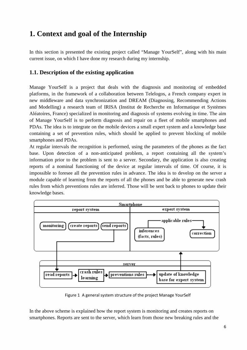
1.1. Description of the existing application Manage YourSelf is a project that deals with the diagnosis and monitoring of embedded platforms, in the framework of a collaboration between Telelogos, a French company expert in new middleware and data synchronization and DREAM (Diagnosing, Recommending Actions and Modelling) a research team of IRISA (Institut de Recherche en Informatique et Systèmes Aléatoires, France) specialized in monitoring and diagnosis of systems evolving in time. The aim of Manage YourSelf is to perform diagnosis and repair on a fleet of mobile smartphones and PDAs. The idea is to integrate on the mobile devices a small expert system and a knowledge base containing a set of prevention rules, which should be applied to prevent blocking of mobile smartphones and PDAs. At regular intervals the recognition is performed, using the parameters of the phones as the fact base. Upon detection of a non-anticipated problem, a report containing all the system’s information prior to the problem is sent to a server. Secondary, the application is also creating reports of a nominal functioning of the device at regular intervals of time. Of course, it is impossible to foresee all the prevention rules in advance. The idea is to develop on the server a module capable of learning from the reports of all the phones and be able to generate new crash rules from which preventions rules are inferred. Those will be sent back to phones to update their knowledge bases.

Figure 1 A general system structure of the project Manage YourSelf

In the above scheme is explained how the report system is monitoring and creates reports on smartphones. Reports are sent to the server, which learn from those new breaking rules and the

7

human expert infer preventions rules. Those rules update the knowledge base of the expert system, which makes corrections to avoid blocking of mobile smartphones.

1.2. The main current issues

Manage YourSelf was first developed in the academic year of 2009-2010, by INSA’s students (Institut National des Sciences Appliquées de Rennes). In the first variant of the software, the learning process from the server was made using decision trees. Today, the objective is to upgrade this part of the software so that it will be able to update knowledge bases on the fly. As reports are created at regular intervals of time when is reported a nominal functioning of a device and at irregular intervals when it is reported a problem, the number of reports coming at a time is a random number, because sets of reports are sent to the server at regular intervals of time. Knowing the previous fact and that we want an up-to-date knowledge base on each device, the learning process should be an online process learning, who is able to modify the set of rules each time a new set of reports is received. As we talk about long-term monitoring, it is impossible to store all reports because of the fact that the report database will grow fast and issues of storage space will rise. On the other hand, concepts could change in time; it is the so called concept drift. It may happen if devices are upgraded in terms of software and hardware. Therefore, old reports should not be considered in the learning process, to avoid the detection of erroneous concepts. Hence, an incremental learning system with partial instance memory is required.

2. Previous work on machine learning In this chapter is presented an overview of the work done for machine learning task, along with its importance, and current problems raised by real world situations in incremental learning approaches. Machine learning is a branch of artificial intelligence that allows computers to infer behaviors based on empirical data, or more simple said, to generalize from the given examples. Machine learning [5] usually refers to the changes in systems that perform tasks associated with artificial intelligence (AI). Such tasks involve recognition, diagnosis, planning, robot control, prediction, etc. Here are three main reasons why machine learning is important:

• Some tasks cannot be defined well except by example; that is, we might be able to specify input/output pairs but not a concise relationship between inputs and desired outputs

• It is possible that important relationships and correlations are hidden among large amount of data. Machine learning methods can often be used to extract these relationships (data mining).

• Environments change over time. Machines that can adapt to a changing environment would reduce the need for constant redesign.

8

2.1. Batch learning vs. incremental learning

Formally, a data stream is an ordered sequence of data items read in increasing order. In practice, a data stream is an unbounded sequence of items predisposed to both noise and concept drifts, and received at a so high rate that each one can be read at most once. Several different representations have been used to describe concepts for supervised learning tasks:

-Decision Trees -Connectionist networks -Rules -Instance-based

Batch-learning systems examine all examples one time (both positive and negative) before making any attempt to produce a concept description, that generally is not further modified. Incremental systems, on the other hand, examine the training examples one at a time, maintaining a “best-so-far” description, which may be modified each time a new example arrives [6]. Any batch learning algorithm can be used in an on-line fashion by simply storing all past training examples, adding them to new ones, and re-applying the method. Disadvantages of running algorithms in a temporal-batch manner include the need to store all training examples, which leads to increased time for learning and to difficulty in recovering when concept change or drift. Another major problem is the impossibility to store all those examples, because the memory is limited. A problem of incremental learning occurs if early examples processed by the system are not representative of the domain or are noisy examples. Examples are processed in an ordered way, depending on the time they arrive in the system. Therefore, they have an order dependence, which will tend to direct learning away from the required concept if current processing examples are not representative. Hence, any incremental method will need to include some old representative examples in a memory to correct this effect. The rest of the paper is focusing over the partial memory systems, because results from past studies suggest that learners with partial instance memory react more quickly to drifting concepts than do learners storing and modifying only concept descriptions [2,7] and require less memory and learning time than do batch learning algorithms.

2.2. Definitions and generalities of incremental learning Scalable learning algorithms are based on decision trees, modeling the whole search space, but it is not a good practice for incremental learning because data stream may involve to rebuild on out-of-date sub-tree which will considerable increase the computational cost. Rule induction is different to decision tree based algorithms in that the whole search space is not modeled and the new queries are classified by voting. A common approach within incremental learning to extract the concepts to be learned consist in repeatedly applying the learner to a sliding window of w examples, whose size can be dynamically adjusted whenever target function starts to drift.

9

Another approach consists in weighting the training examples according to the time they arrive, reducing the influence of old examples. Both approaches are partial instance memory methods.

In the problem of classification, an input finite data set of training examples is given T={e1,...,en}. Every training example is a pair (x,y), x is a vector of m attribute values (each of which may be numeric or symbolic), y is a class (discrete value named label). Under the assumption there is an underlying mapping function f so that y = f(x), the goal is to obtain a model from T that approximates f as f’ in order to classify or decide the label of non–labeled examples, named queries, so that f’ maximizes the prediction accuracy. The prediction accuracy is defined as the percentage of examples well classified. Within incremental learning, a whole training set is not available a priori but examples arrives over time, normally one at a time t and not time–dependent necessarily (e.g., time series). Despite online systems continuously review, update, and improve the model, not all of them are based on an incremental approach. According to the taxonomy in [1], if Tt= {(x,y)| y = f(x )} for t =< 1,...,∞ >, now f’t approximates f. In this context, if an algorithm discards f’t−1 and generates f’t from Ti, for i =< 1,...t>, then it is on–line batch or temporal batch with full instance memory. If the algorithm modifies f’t using f’t−1 and Tt, then it is purely incremental with no instance memory. A third approach is that of systems with partial instance memory, which select and retain a subset of past training examples to use them in future training episodes.

2.3. Classification of incremental learning approaches

Figure 2 A classification of on-line learning systems in term of concept memory and instance memory

On-line learning systems must infer concepts from examples distributed over time and such systems can have two types of memory:

• Memory for storing examples • Memory for storing concept descriptions

10

A full instance memory is an instance-based method that stores all previously encountered training cases (all examples). Incremental systems with partial instance memory, select and maintain a portion of the training examples from the input stream, using them in future training episodes, for example IB2 stores those examples that it misclassifies. Finally, those systems, which learn from new examples and then discard them, are called systems with no instance memory. In terms of concept memory, most systems are full concept memory; they form concept descriptions from training examples and keep them in memory until altered by futures training episodes. Some others are partial concept memory, as FAVORIT [8] who induces trees from examples, but maintains a weight for each node of the tree. If not reinforced by incoming training examples, these weights decay and nodes are removed from the tree when their weights are below a threshold. Finally, some learners do not form concept descriptions that generalize training examples; those are called learners with no concept memory, as IB2.

2.4. Current issues in incremental learning

As it is said earlier, a problem of incremental learning occurs if early examples processed by the system are not representative of the domain or are noisy examples. This order dependence will tend to direct learning away from the required concept, so any incremental method will need to include some examples in a memory to correct for this effect. Therefore an important issue of partial instance memory learners is how such learners select examples from the input stream. Those selection methods can be classified in three main approaches:

• select and store representative examples (near the center of a cluster)[9,10] • remember consecutive sequence of examples over a fixed [11] or changing windows of

time[2] • keep extreme examples that lie on or near the boundaries of current concept

descriptions[7,9]

Along with the ordering effects, incremental learning from real-world domains faces two problems known as hidden context and concept drift, respectively [2]. The problem of hidden context is when the target concept may depend on unknown variables, which are not given as explicit attributes. In addition, hidden contexts may be expected to recur due to cyclic or regular phenomena (aka recurring contexts) [12]. The problem of concept drift is when changes in the hidden context induce changes in the target concept. In general, two kinds of concept drift depending on the rate of the changes are distinguished in the literature: sudden (abrupt) and gradual. In addition, changes in the hidden context may change the underlying data distribution, making incremental algorithms to review the current model in every learning episode. This latter problem is called virtual concept drift [2]. There are 2 common approaches that can be applied altogether to detect changes in the target concept:

- Repeatedly apply the learner to a single window of training examples whose size can be dynamically adjusted whenever target function start to drift (FLORA)

- Weighting the training examples according to the time they arrive, reducing the influence of old examples (AQ-PM)

11

3. Representative approaches in incremental learning

In this section, we will present different solutions proposed for incremental learning, as well as the non-incremental AQ21 algorithm, which is use later in my proposed incremental method. The way incremental learning is performed depends on what kinds of examples are stored from previous steps, to use in following steps. It also depends on the algorithm itself, if it use only examples stored or if it use also previous rules achieved.

3.1. FLORA family

The FLORA systems, which are designed to learn concepts that change or drift, select and maintain a sequence of examples from the input stream over a window of time. These systems size this window adaptively in response to severe decreases in predictive accuracy or to increases in concept complexity, measured by the number of conditions in a set of conjunctive rules. It also takes the advantage of situations where context reappears, by storing old concepts of stable situations for later use. The learner trusts only the latest examples; this set is referred to as the window. Examples are added to the window as they arrive, and the oldest examples are deleted from it. Both of these actions (addition and deletion) trigger modifications to the current concept description to keep it consistent with the examples in the window. The main techniques constituting the basic FLORA method are representation of descriptions in the form of three description sets (ADES, NDES, PDES) that summarize both the positive and the negative information, a forgetting operator controlled by a time window over the input stream and a method for the dynamic control of forgetting through flexible adjustment of the window during learning. The central idea is that forgetting should permit faster recovery after a context change by getting rid of outdated and contradictory information. In the simplest case, the window will be of fixed size, and the oldest example will be dropped whenever a new one comes in. The extensions of the learning algorithm should decide when and how many old examples should be deleted from the window ('forgotten') and a strategy that maintains the store of current and old descriptions. The three description sets are as follow:

• ADES (accepted descriptors) is a set of all descriptions that are consistent and it is used to classify new incoming examples.

• NDES (negative descriptors) is a consistent description of the negative examples seen so far. It is used to prevent over-generalizations of ADES.

• PDES (potential descriptors) is a set of candidate descriptions, who acts as a reservoir of descriptions that are currently too general but might become relevant in the future. It is complete, but not consistent. Therefore it is matching positive examples, but also some negative ones.

The algorithm counts how many positive examples are covered by a rule in ADES, respectively PDES and also the number of negative examples covered by a rule in NDES, respectively PDES. The counters are updated with any addition to or deletion from the window and are used to decide when to move an item from one set to another, or when to drop them. In any case, items are retained only if they cover at least one example in the current window. More precisely,

12

modifications to the window may affect the content of the description sets by: adding a positive example to the window; adding a negative example to the window or forgetting an example. There are three possible cases for ADES when a new positive example is added: if the example matches some items, the counters are simply incremented; otherwise, if some item can be generalized to accommodate the example without becoming too general, generalization is performed. Finally, if none of those previous cases are found, the description of the example is added as a new description to ADES. For the addition of a negative example, same type of operations are performed, but with the NDES set and when forgetting an example those counters are decremented [14]. The only generalization operator used is the dropping condition rule [15], which drops attribute-value pairs from a conjunctive description item and no specialization operator is used in this framework. FLORA2 possesses the ability to dynamically adjust the window to an appropriate size during the learning process, by means of heuristics. The occurrence of a concept change can only be guessed at. A good heuristic for dynamic window adjustment should shrink the window and forgot old examples, when a concept drift seems to occur. Window Adjustment Heuristic decreases the window size by 20% if a concept drift is suspected and keep the window size fixed when the concept seems stable. The window size is decreased by 1 if the hypothesis seems to be extremely stable, but if the current hypothesis seems just sufficiently stable, the window size is simply left unchanged. Otherwise the window should gradually grow, increasing the window size by 1, until a stable concept description can be formed. A possible concept drift may be signal by a serious drop in Acc (current predictive accuracy) or an explosion of the number of description items in ADES. Differences between extremely stable, stable enough and unstable are made by some thresholds over those two mathematical measures computed on every window. FLORA3 is an extension of FLORA2 that stores concepts of stable situations for later use. After each learning cycle, when the learner suspects a context change, it examines the potential of the previously stored descriptions to provide better classifications. Based on the result, the system may either replace the current concept description with the best of the stored descriptions, or start developing an entirely new description. The best candidate is determined through a simple heuristic measure, which sometimes leads to an inappropriate candidate being chosen. Conversely, when a stable concept hypothesis has been reached, it might be worthwhile to store the current hypothesis for later reuse, unless there is already a stored concept with the same set of ADES descriptions. FLORA4 is designed to be particularly robust with respect to noise in the input data. It uses a refined strategy based on the monitored predictive performance of individual description items to deal with the problem of noisy data. FLORA4 drops the strict consistency condition and replaces it with a “softer” notion of reliability or predictive power of generalizations. The main effect of the strategy is that generalizations in ADES and NDES may be permitted to cover some negative or positive examples, if their overall predictive accuracy warrants it; and PDES is seen as a reservoir of alternative generalizations that are recognized as unreliable at the moment, either because they cover too many negative examples, or because the absolute number of examples they cover is still too small.

13

3.2. AQ family

AQ11-PM is an on-line learning system with partial instance memory, which selects extreme examples from the boundaries of induced concept descriptions under the assumption that such examples enforce, map, and strengthen these boundaries. IB2, one of its precedents, which is presented in the next section, includes an example into its store if the algorithm misclassifies the example; otherwise discard the example. As the learner processes examples, most misclassifications occur at the boundary between concepts, so IB2 tend to keep examples near this interface. The difference between IB2 and AQ11-PM is that the AQ11-PM use induced concept descriptions to select extreme examples. Another precedent, the AQ-PM system [7] induces rules from training examples and selects examples from the edges of these concept descriptions. It is a temporal-batch learner, so it replaces the current rules with new ones induced from new examples and those held in partial memory. AQ11-PM identifies extreme examples from the training set. In the scheme of reevaluating after each episode, if an example held in partial memory fails to fall on the boundary of the new concept descriptions, then the example is removed. It is called implicit forgetting process. Explicit forms of forgetting can be useful in context of changing concepts for properly maintaining partial memory and may include policies that remove examples if they become too old or if they have not occurred frequently in the input stream. Next is presented a general algorithm for incremental learning with partial instance memory for static and changing concepts [7, 13]:

1. sets of input data at each instance of time t = 1…n

2. concept={}

3. partial_memory = {}

4. for t=1…n

5. if data <>{} then

6. missed t= find missed_examples (concept t-1, data t)

7. training_set t= partial_memory t-1 U missed t

8. concept t= learn (training_set t, concept t-1)

9. partial_memory‘ t= select_examples_extreme (training_set t, concept t)

10. partial_memory t= maintain_examples (partial_memory‘ t, concept t)

11. end if

12. end for

The input to the algorithm is some number of data sets (n), one for each time step; and each data set has a random number of examples. An incremental learner uses these examples and its current concept descriptions to form new concept descriptions, whereas a temporal-batch learner uses only the extreme examples and any new training examples.

14

In the set called “partial_memory‘ t” are selected those examples in the current training set from the boundaries of the concept descriptions. Extreme examples can be identified from the current training set or only among the new examples from the input stream and then accumulating these with those already stored in partial memory. If a concept drift is detected, old examples may need to be forgotten and if an example appears frequently, it should be weighted more heavily than others; those updates are made in the function maintain_examples. The learning element of the AQ algorithm begins by randomly selecting a positive training example called the seed, which is then generalizes maximally so as not to cover any negative example. Using the rule produced by this process, the algorithm removes from the training set those positive examples that rule covers, and then repeat until covering all positive examples. Furthermore, this procedure results in a set of rules that are complete and consistent, meaning that rules of a given class cover all of the examples of the class and cover none of the examples of other classes. The predecessor of AQ11-PM, called AQ11 is an extension of the AQ system, but rather than operating in a batch mode, AQ11 incrementally generates new rules using its existing rules and new training examples. AQ11 focuses on a rule of the positive class, if it covers a negative example then it specializes the rule. After that, it combines specialized positive rules and the new positive training examples and use them in AQ to generalize. AQ11 retains none of the past training examples, therefore is a no instance memory learner, and relies only on its current set of rules. Hence, rules will be complete and consistent with respect to the current examples only. AQ11-PM selects examples near the boundaries of a concept, but uses concept descriptions to select examples on their boundaries. It is actually AQ11 with a post-processing step to learning, in which extreme examples are computed and then included in the next training set. Algorithm for extreme examples selection:

1. for each rule

2. specialize rule

3. for each selector in the rule

4. generalize rule

5. select matched examples

6. extreme examples = extreme examples U matched examples

7. end for selector

8. end for rule

The specialize operator removes intermediate attribute values for each of its selectors and the generalize operator adds intermediate values for the selector chosen in the specialized rule. Rules carve out decision region in the partition space, rather than partitioning the space like decision trees. Consequently, there may be no rule that is true for a given instance. Therefore, flexible matching is used, by computing the degree of match between the new example and each of the rules and selecting the highest one.

15

From AQ11 the AQ systems were furthermore developed. Nowadays, the last version is AQ21 which perform natural induction, meaning that it generate inductive hypotheses in human-oriented forms that are easy to understand, but it is not an incremental algorithm, it operates in a batch mode. AQ21 integrates several new features: optimize patterns according to multiple criteria, learn attributional rules with exceptions, generate optimized sets of alternative hypotheses and handle data with unknown, irrelevant and /or non-applicable values. AQ21 has three modes of operation: Theory Formation (TF), Approximate Theory Formation (ATF) and Pattern Discovery (PD). TF generates consistent and complete (CC) data generalizations (similar to the AQ11 algorithm). ATF optimizes the CC description to maximize a criterion of description utility; therefore, it may be partially inconsistent and/or incomplete, but it has the description simplicity. PD produces attributional rules that capture strong regularities in the data, but may not be fully consistent or complete with regard to the training examples.

RS = null

While P is not empty

Select a seed example, p, from P

Generate a star or an approximate star G(p, N)

Select the best k rules from G according to LEF, and include them in RS

Remove from P all examples covered by the selected rules

Optimize rules in RS

Assemble a final hypothesis, a set of alternative hypotheses, or patterns from all rules in RS

Figure 3 Top-level learning algorithm in AQ21

The above algorithm applies to all three modes, but in ATF and PD modes at each step of star generation it optimizes rules according to a rule quality measure, Q(w), instead of generating consistent rules. Thus, the key part of the algorithm is the generation of a star G(p, N), for the given seed(a random positive example) p, against the set of negative examples, N. In TF mode, a star is a set of maximally general consistent attributional rules that cover the seed but do not cover any negative examples, and ATF and PD modes, the rules may be partially inconsistent. In each mode, rules are selected from stars, maximizing a quality measure, defined by the user using a Lexicographical Evaluation Functional (LEF) [15], a multi-criterion measure of rule preference, defined by selecting a subset of elementary criteria from a list of such criteria predefined in AQ21.[18] While TF is oriented toward error-free data, ATF is most useful when a small amount of errors may be present or the user seeks only approximate, but a simple data generalization and PD where strong regularities in the data need to be capture. In TF mode, where consistency must be guaranteed, the program adds negative examples to the list of exceptions, if such examples are infrequent in comparison to the examples covered by the rule, but would introduce significant complexity in order to accommodate them. If all exceptions

16

from the rule can be described by one conjunctive description, such a description is created and used as the exception part, otherwise, an explicit list of examples that are exceptions is used. A rule in AQ21 learning uses a richer representation language than in typical rule learning programs, in which conditions are usually limited to a simple form [<attribute><relation><attribute_value>]. Here the basic form of an attributional rule is: CONSEQUENT <= PREMISE where both CONSEQUENT and PREMISE are conjunctions of attributional conditions in the form: [L rel R: A] where L is an attribute, an internal conjunction or disjunction of attributes, a compound attribute, or a counting attribute; rel is represented by one of =, :, >, <, ≤, ≥, or ≠, and R is an attribute value, an internal disjunction of attribute values, an attribute, or an internal conjunction of values of attributes that are constituents of a compound attribute, and A is an optional annotation that lists statistical information about the condition (e.g., p and n condition coverage, defined as the numbers of positive and negative examples, respectively, that satisfy the condition). AQ21 can be set to learn rules with exceptions, in the form: CONSEQUENT <= PREMISE |_ EXCEPTION : ANNOTATION where EXCEPTION is either an attributional conjunctive description or a list of examples constituting exceptions to the rule and ANNOTATION lists statistical and other information about the rule, such as numbers of positive and negative examples covered, the rule’s complexity, etc. AQ21 can learn alternative hypotheses in two steps. In the first step, more than one rule is selected from each star, thus different generalizations of the seed are kept (when k > 1 in the algorithm in Figure 1). In the second step, these rules are assembled together to create alternative hypotheses, ordered based on user-defined criteria. Details of the algorithm for learning alternative hypotheses are presented in [19]. AQ21 is able to handle data with unknown, irrelevant and /or non-applicable values. Unknown denoted by a “?” in the training dataset, is given to an attribute whose value for a given entity exists, but is not available in the given data base for some reason. For example, the attribute may not have been measured for this entity, or may have been measured, but not recorded in the database. Two internal methods for handling Unknown values are implemented in AQ21: (L1), which ignores the extension-against operation (a basic generalization operation in AQ [18]) for attributes with missing values, and (L2), which treats “?” as a regular value in the examples, but avoids examples with a “?” when selecting seeds. When extending a seed against a missing value, it creates a condition: [xi≠?], regardless of the value of attribute xi in the seed. Not-applicable, denoted by an “NA,” is given to an attribute that does not apply to a given entity, because its value does not exist. Irrelevant values, denoted by an “*”, indicate that values exist, but an attribute is considered irrelevant to the learning problem, to the concept (class) to be learned, or to the particular event.

17

The following table summarizes and compares the methods outlined above, considering the essential points of algorithms.

Method Type of stored

examples

Type of

generalization

Number of

user parameter

How drift is

managed

AQ11-PM extreme examples

located on concepts

boundaries

generalizes

maximally

few hardly detected

AQ21 extreme examples

located on concepts

boundaries

depends on

operation mode

average -

FLORA2 a sliding window with

last examples

generalizes when

needed

few quickly detected

FLORA3 a sliding window with

last examples

generalizes when

needed

few quickly detected and

current concepts

changing

FLORA4 a sliding window with

last examples

generalizes when

needed

few quickly detected,

current concepts

changing and

robustness to noise

Table 1 A comparison between the main incremental methods presented and the batch mode algorithm AQ21

3.3. Others

In the following subsection, some others approaches are presented, due to the fact that from each we use small parts to develop our own approach. From IBL family and FACIL we merge the similarity function with, respectively, the growth of a rule function to create a new way of computing distance to retrieve border examples. FACIL, on the other hand, along with DARLING were also studied for their forgetting mechanisms approach, which inspired us in creating our own. IBL family Instance-based learning (IBL) [20] algorithms are derived from the nearest neighbor pattern classifier. They save and use specific selected instances to generate classification predictions. Most supervised learning algorithms derive generalizations from instances when they are presented and use simple matching procedures to classify subsequently presented instances. IBL algorithms differ from those in the fact that it does not construct explicit abstractions such as decision trees or rules. They save examples and compute similarities between their saved examples and the newly presented examples.

18

IB1 algorithm is the simplest instance-based learning algorithm. It is identical to the nearest neighbor algorithm, except that it normalizes its attributes ranges, process instances incrementally and has a simple policy for tolerating missing values. Below is presented the IB1 algorithm:

Figure 4 IB1 algorithm

The concept description (CD) is the set of saved examples which describe the current classification. The similarity function used here and also for following algorithms (IB2 and IB3) is:

Where examples are described by n attributes, each is noted ix . The function f is defined as:

attributesymbolicyx

attributenumericyxyxf

ii

iiii

),(

,)(),(

2{≠−

=

Missing attribute values are assumed to be maximally different from the value present and if both are missing then the function f yields 1. IB2 is identical to IB1, except that it saves only misclassified examples. In noisy and/or sparse databases IB2 performances rapidly degrades comparing to IB1. In noisy databases, this is happening because most of the noisy examples are stored; as for the sparse database it is because most of the examples appeared to be near boundary. Sparse and dense are a property of the values of an attribute. Data is normally stored in a mixture of sparse and dense forms. If no value exists for a given combination of dimension values, no row exists in the fact database; and sparse database consist in having few combination of dimension values. On the other part, a database is considered to have dense data if there is a high probability to have one row for every combination of its associated dimension.

19

Figure 5 IB2 algorithm

IB3 is an extension of IB2 which tolerate noise. It employs a simple selective utilization filter (Markovitch & Scott, 1989) to determine which of the saved examples should be used to make classification decisions. IB3 maintains a classification record for each saved example (number of correct and incorrect classification attempts) and employs a significance test to determine which examples are good classifiers and which ones are believed to be noisy. The latter are discarded from the concept description. [Annex1] From empirical results it is seen that IB3 can significantly reduce IB1’sstorage requirements and does not display IB2’s sensitivity to noise. Furthermore, it has improved performances in sparse databases than IB2. On the other hand, IB3’s learning performances is highly sensitive to the number of irrelevant attributes used to describe examples. Its storage requirements increase exponentially and its learning rate decrease exponentially with increasing dimensionality. A possible extension is to locate irrelevant attributes and ignore them; this will effectively reduce the dimensionality of the instance space. IBL algorithms incrementally learn piecewise-linear approximations of concepts in contrast with algorithms that learn decision tree or rules which approximate concepts with hyper-rectangular representations. A summary of the problems rise by IBL algorithms can be sketch as follow:

-computationally expensive (if they save all training examples)

-intolerant of noise attributes (IB1 and IB2)

-intolerant of irrelevant attributes

-sensitive to the choice of the algorithm’s similarity function

-no natural way to work with nominal-valued attributes or missing attributes

-provide little usable information regarding the structure of the data

20

FACIL Fast and Adaptive Classifier by Incremental Learning (FACIL) is an incremental rule learning algorithm with partial instance memory that provides a set of decision rules induced from numerical and symbolic data streams. It is based on filtering the examples lying near to decision boundaries so that every rule may retain a particular set of positive and negative examples. Those sets of boundary examples make possible to ignore false alarm with respect to virtual drift and hasty modifications. Therefore, it avoids unnecessary revisions. The aim of FACIL is to seize border examples up to a threshold is reached. It is similar to AQ11-PM system, which selects positive examples for the boundaries of its rules and store them in memory; but the difference consist in the fact that FACIL does not necessary save extreme examples and rules are not repaired every time they become inconsistent(they cover negative examples as well).

Figure 6 FACIL – growth of a rule

In the above definition is computed a distance between the rule r and the example e. There is just

a notation which is not explained in the figure, it is which represent the cardinal of the

symbolic attribute domain . This approach stores 2 positive examples per negative example covered by a rule. It has no global training window used; each rule handles a different set of examples and has a rough estimation of the region of the space that it covers. If the support of a rule is greater than a threshold, than the rule is removed and new rules are learned from its set of examples covered. Examples are also rejected when they do not describe a decision boundary. The algorithm uses 2 different forgetting heuristics to remove examples so that it limited the memory expansion:

21

-explicit: Delete examples that are older than a user defined threshold

-implicit: Delete examples that are no longer relevant as they do not enforce any concept description boundary

DARLING Density-Adaptive Reinforcement Learning (DARLING) [10] is identifying regions of the parameter space where the lower-bound probability of succeeding is above some minimum probability required for the task. It produces a classification tree that approximates those regions. DARLING algorithm is inspired from decision tree approaches and it has a technique to delete old examples using exponential weight-decay based on a nearest-neighbor criteria. The weight of an example is decayed and deleted when it goes below some minimum value, and is superseded by the newer example that led to its deletion. New observations decay only their neighbors. In order to store only a bounded number of examples at any given time, DARLING uses a mechanism which delete old examples. This mechanism is implemented by associating a weight to each example. Each weight is decremented at a rate proportional to the number and proximity of succeeding examples to the corresponding example. When a given example’s weighting falls below some threshold value, it is deleted from the learning set.

3.4. Conclusions of previous work

To briefly recapitulate this chapter, I will show the most important characteristic of each approach presented above. In FLORA the general approach assumes that only the latest examples are relevant and should be kept in the window and that only description items consistent with the examples in the window are retained. This may lead sometimes to erroneous deletion of concepts descriptions that are still available. The incremental approach of AQ systems stores older useful concept description and it also keep older examples, which are located on concepts description borders, than FLORA does. Therefore, results of AQ11-PM are generally increased than those of FLORA2 [1]. Despite those favorable results, it has some disadvantages. For instance, extreme examples may cause overtraining, so the rules while simpler are not as general and it also has not incorporated any adaptive forgetting mechanisms. IB systems do not form concept descriptions that generalize training examples. They just keep specific examples, which are used directly to form predictions, by computing similarities between those saved examples and the newly ones. Those approaches are expensive computationally algorithms and they depends on their similarity function.

22

FACIL is similar to the AQ11-PM approach, just that it stores both positive and negative examples, which are not necessary extreme. Furthermore, it does not repair rules each time they become inconsistent. But, the main disadvantage of this algorithm is the presence of many user defined parameters, which are not so easy to tune. DARLING is creating a classification tree, which make this approach a computationally expensive one. The interesting feature owned by this algorithm is its forgetting mechanism, which delete old examples based on proximity examples. This technique incorporates a small disadvantage, by the fact that some outdated concepts may not be deleted if the drift is sudden. Incremental learning is more complex than batch learning, because learners should be able to distinguish noise from actual concept drift and quickly adapt the model to new target concept. Incremental learning was studied in this paper because here is no need to re-examine all the instances at every learning step. Furthermore, partial-memory learners were searched, because those notably decrease memory requirements and learning times. As a drawback, they tend to lightly reduce predictive accuracy.

4. Contribution

This chapter presents the framework on an instance-based learning algorithm, with partial instance memory, which extends the AQ21 algorithm by transforming it into an incremental approach. As we presented in chapter 2, the main issue is to update the Manage YourSelf project’s module, which is capable of learning from smartphone’s generated reports. Our proposed approach is an attempt to map on Manage YourSelf current issue better than previous works. As devices may be upgraded in terms of software and hardware, concepts could change in time and we need to track those concept drift. Hence, our proposed method is also an attempt to pursue changes in concept description.

4.1. Overview of the internship

It is needed an approach to upgrade the current classification method used on the server module of the Manage YourSelf project. Therefore, the task studied in this internship is supervised learning or learning from examples. More specifically, we focus on the incremental on which the only input is a sequence of examples. In the context of Manage YourSelf project, those examples are functioning reports generated by each smartphone or PDA of the mobile fleet. As reports came to server at regular intervals of time, in sets of different size, the formal incremental approach, which imply to modify the current concept description for each new incoming example, is not suitable for our needs. Knowing the previous fact and that we want an up-to-date concept description for the crash functioning reports, the learning process should be more a batch learning algorithm used in an on-

23

line fashion. It is an online process learning, who is able to modify the set of rules each time a new set of reports is received. Below I present what motivated this work and which are the challenges raised by classifying smartphone’s functioning reports.

4.1.1. Motivation

The Manage YourSelf project needed an upgrade to its module of classifying functioning reports generated by the fleet of smartphones and PDA’s and all the study of previous works didn’t mapped well on the present configuration of the project. Our work is an attempt to create a framework which maps better on Manage YourSelf current issue. It is needed only consistent rules of crash reports, presented in a form resembling natural language description. It is due to the fact that in the following module of Manage YourSelf project, a human expert will use those to create rules of crash prevention. Therefore, our approach is based only on consistent concept descriptions, expressed in way easy to understand and interpret. A rule is said consistent when it does not cover any negative example. The aim is to retrieve a part of consistent rules which cover the majority of crash report examples and to model those in a conjunctive normal form (CNF) [22]. In addition, we are talking about long-term monitoring and here, it is impossible to store all reports because of the fact that the report database will grow fast and we could not have an infinite storage. Along with the increase of reports stored, the learning time will also increase significantly and our aim is to have a constant learning time.

4.1.2. Challenges

As the system must operate continuously and process information in real-time, memory and time limitations make batch algorithms unfeasible due to the amount of data received at a higher rate than they can analyze. Therefore, to achieve this goal we must take in count only few old examples. So the first challenge is to reduce the storage requirements and the processing time, but if we would consider only the new income examples, then we are likely to obtain erroneous rules due to noise and unreal drift. The examples between classes, also known as border ones, are the only ones needed to produce an accurate approximation of the concept boundary. The other examples do not distinguish where the concept boundary lies. Therefore, a great reduction in storage requirements is gained by saving only informative border examples. Unfortunately, this set is not known without complete knowledge of the concept boundary. However, it can be approximated at each learning step by examples lying on current concept description boundaries. Furthermore, real-world data streams are not generated in stationary environments, this involves the need to track drift concept and repeatedly to change the current target concept. Hence, incremental learning approaches are required for detecting changes in the target concept and adapt the model to the new target concept. To achieve correct concept description, without regarding outdated examples, which leads to erroneous rules, we used the approach of applying weights to training examples according to the time they arrived in the system. This method is reducing the

24

influence of old examples in time and it is called a partial instance memory method, which implies an explicit forgetting, involving age forgetting mechanism. Hence, is required a classification system based on decision rules, that may store up-to-date border examples to avoid erroneous rule detection and to track concept drifts.

4.2. Simulation of input data

For generating input data, it was used a data simulator made by a group of INSA students, last year, with a batch of modifications to fit with our input data needs. Presenting smartphone models used Through this program, some smartphones behavior was simulated. We had chosen 8 different types of smartphone’s models: Galaxy Mini, Galaxy S2, Xperia Pro, Xperia Mini, IPhone S4, Omnia7, Lumia 900, Lumia 800; from 4 different brands: Samsung, Sony, Nokia and Apple. Which incorporate 3 different types of operation system: Android, IOS and Windows Mobile Phone.

Type of Operation System Brand Model

Android

Samsung

GalaxyMini

Galaxy S2

Sony

Xperia Pro

Xperia Mini

IOS Apple IPhone 4S

MicrosoftWindowsPhone Samsung Omnia 7

Nokia

Lumia 900

Lumia 800

Table 2 Criterions to divide and characterize the fleet of smartphones

Presenting smartphone attributes

Each model of smartphone has its own characteristics. Some of those were accurate taken from an internet website [23] which has an up-to-date database of mobile features. Others were computed to be proportional with those characteristic to the model GalaxyS, of the Samsung brand, operating on the Android operating system. Those proportionalities were made because we couldn’t find nowhere some features that we consider to be important and also because for Galaxy S we had the exact values of those features, by measuring these directly on a Galaxy S smartphone through a set of specific applications. Among the accurate characteristic found on the website we used: memory size (RAM and ROM), battery amperage and battery life on stand-by and also on talk time. One of most important characteristic that we consider, but we couldn’t find anywhere, is the initial memory, both for RAM and for ROM, which we approximate by making a proportionality with the initial memory of the Galaxy S. This initial memory is the size of memory employed for the operation system installed on the smartphone and some few application which came with it and

25

are opened each time the system reboot. The RAM size is taking this value each time is simulated a reboot or a shut-down of the smartphone operation system. The ROM size, in the other hand, is taking this value only one time at the simulation start. There features are presented in the following table. As for the ROM memory we have chosen randomly one of the possible values when the model disposed of an option list, it is presented in the table by bolding the chosen values.

Model OS version RAM size RAM

initial

ROM size ROM

initial

Battery Stand-by Talk

time

Galaxy S Android 2.1 512 MB 190 MB 2000 Mb

32000 MB

300 MB 1500 mAh 750 h

45000 m

810 m

GalaxyMini Android 2.2 384 MB 150 MB 160 Mb

2000 Mb

32000 MB

300 MB 1200 mAh 600 h

36000 m

600 m

Galaxy S2

(i9100)

Android 2.3 1000 MB 320 MB 16000 Mb

32000 MB

600 MB 1650 mAh 710 h

42600 m

1100 m

Xperia Pro Android 2.3 512 MB 200 MB 320 Mb

1000 MB

8000 MB

32000 MB

400 MB 1500 mAh 430 h

25800 m

415 m

Xperia

Mini

Android 2.3 512 MB 200 MB 512 MB

2000 MB

4000 MB

32000 MB

300 MB 1200 mAh 340 h

20400 m

270 m

IPhone 4S IOS5 512 MB 250 MB 16000 Mb

32000 MB

64000 Mb

500 MB 1432 mAh 200 h

12000 m

840 m

Omnia 7 MWP 7 512 MB 220 MB 8000 Mb

16000 Mb

400 MB 1500 mAh 390 h

23400 m

340 m

Nokia 500 Symbian

Anna

256 MB 170 MB 512 MB

2000 MB

300 MB 1110 mAh 500 h

30000 m

420 m

Lumia 900 MWP 7.5 512 MB 200 MB 16000 MB 350 MB 1830 mAh 300h

18000 m

420 m

Lumia 800 MWP 7.5 512 MB 200 MB 16000 MB 350 MB 1450 mAh 265 h

15900 m

780 m

Table 3 Smartphones characteristics

From previous characteristics we have extracted some attributes which are used to simulate smartphone behavior, we called those general attributes:

1. Brand 2. Model 3. Type of the operation system 4. Operation system version 5. RAM size 6. ROM size

26

7. Battery level 8. RAM level of usage 9. ROM level of usage

First 6 attributes are the ones retrieved from the above tables. The battery level represents the percentage of battery life remaining. The level of usage of the RAM memory is the number of thousandth parts from the RAM memory used and the level of usage of the ROM memory represents the number of MB used from it. Presenting smartphone applications used Besides those attributes, there are also attributes of the type application, which specify if an application is running or not. Those attributes are in the form of app_[name_of_application]. The total number of possible applications is 32. These are listed below:

1. Appli_GSM 2. Appli_Call 3. Appli_GPS 4. Appli_WIFI 5. Appli_Camera_video 6. Appli_Camera_photo 7. Appli_vibration 8. Appli_Clock 9. Appli_syncro 10. Appli_Bluetooth 11. Appli_IGO 12. Appli_Birds 13. Appli_Music 14. Appli_Skype 15. FuiteMemoirePhysique 16. FuiteMemoireVive

17. EffaceMemoirePhysique 18. Recharge 19. Appli_Volum1 20. Appli_Volum2 21. Appli_Volum3 22. Appli_Volum4 23. Appli_Luminosity1 24. Appli_Luminosity2 25. Appli_Luminosity3 26. Appli_Luminosity4 27. Appli_Incompatible_MicrosoftWindowsPhone 28. Appli_Incompatible_Android 29. Appli_Incompatible_IOS 30. Appli_Incompatible_Omnia7 31. Appli_Incompatible_Telephone 32. Appli_Incompatible_Apple_GPS

Each application has its own characteristics about how much and what exactly is using from a smartphone properties. We have measured for some applications how much RAM they used on the Galaxy S and we assumed that the same is used for each other model type. After that we have made the translation in per thousand from the total RAM size of each model [Anexe1]. Smartphone\Application Stand-

by

Talk-

time

Skype IGO Music Birds WIFI Camera

Video |Photo

GalaxyS 5 5 16 35 13 11 5 15 5

Table 4 How much RAM in MB smartphones use for some applications

For the usage of the ROM, we assumed that only the following application are increasing it and that for all smartphone’s models those application are taken the same number of MB. The table below presents the amount of MB occupied by those applications each time they are turned on.

27

Application ROM used(MB)

Appli_Bluetooth 15

Appli_syncro 30

Appli_Birds 1

Appli_Camera_video 25

Appli_Camera_photo 5

FuiteMemoirePhysique 50

Appli_Clock 1

Table 5 How much ROM in MB smartphones use for some applications

The only application which release ROM memory is EffaceMemoirePhysique, which discounts from the ROM used 50 MB. Besides the amount of memory used, applications are also using battery. We had measured for some application in how many minutes a percent of battery is used on a Galaxy S and made proportionalities for others smartphones models as below.

Smartphone\Applications Stand-

by

Talk-

time

Skype IGO Music Birds WIFI Camera

Video |Photo

GalaxyMini 360 6 2 3 35 5 20 1 2

Galaxy S2 426 11 3 5 60 7 30 1 2

Xperia Pro 258 4 1 2 15 2 10 1 2

Xperia Mini 204 3 1 1 20 7 10 1 2

IPhone 4S 120 8 2 4 30 5 20 1 2

Omnia 7 234 3 1 1 25 2 10 1 2

Lumia 900 180 4 1 2 36 2 20 1 2

Lumia 800 159 7 2 2 33 5 20 1 2

GalaxyS 450 8 2 3 30 5 20 1 2

Table 6 In how many MINUTES should we discount 1% from battery, for some application per

smartphone model

The functioning of a simulated application is described in Annex2. Applications attributes specify which applications are active and which are inactive. They are symbolic attributes, having just 2 options: running and notrunning. And finally, there are two other attributes, called crash attributes: crash and the type of crash. Crash is giving the state of smartphone, it is a Boolean attribute: false is for normal behavior and true is for a crash. The other attribute is giving the reason of the crash (memory full, battery empty or application crash). As listed above, attributes are both numerical and symbolic and describe smartphones current characteristics and the list of applications running on those. A total of 88 phones where simulated during a period of a month. Each model includes 11 smartphones, which are differentiated by an attribute called numero, that represent a fictive phone number. Each smartphone model has its own rules of crash behavior as seen in Table8. Those will be the rules that we expect to extract after the incremental learning process.

28

Presenting smartphone simulated examples Each example simulated is represented by a set of attribute-value pairs. All examples are assumed to be described by the same set of attributes. A total of n equal 44 attributes exists, which include general attributes, application attributes, crash attributes and the attribute which make the difference between smartphones: numero. In our approach missing attributes are tolerated and their value are marked by “?”. Those missing attributes could be found in case that from a specific type of smartphone we are not able to read its value and also in case when we merge two sets of examples from two smarphones having a different list of applications installed, because for missing application the value is set as unknown and not as not-running. This set of attributes defines a n-dimensional instance space and exactly one of these attributes correspond to the class attribute. A class is a set of all examples in a instance space that have the same value for their class attribute. In this work, we assumed that there is exactly one class attribute (crash) and that classes are disjoint. The simulation was based on some rules describing the crash behavior for each model type. Those rules are classified in five distinct categories:

- general rules: these rules are applied to all models - operation system rules: represents rules applied only on a specific operation system - band rules: are those rules who mapping on a brand - model rule: are rules existing only on certain a model - specific telephone rules: are rules that can exist on all smartphones just that only for few telephones those are presented

In Table8 are shown, for each model, rules that are applied on a smartphone model to simulate his behavior. Each model has 10 smartphones simulated with the first 4 types of rules crash behavior and only one smartphone having all rules applied. Those rules are the one that are expected to be found after applying our incremental learning approach, but as the simulator does not generate all possible combinations of attribute values and therefore we have a sparse database, we do not expect to find exactly those simulated rules. However, due to this sparse data obtained, we expect to achieve rules that represent specializations of those crash behavior rules for the simulated input data. The simulation is generating in 30 days of simulation for each smartphone, approximately 1600 nominal functioning reports and 200 crash reports. Which give a total of almost 1800 functioning reports per month for a smartphone and for all the fleet there is a total of 156945 reports. In the table below all functioning reports are counted and presented in diverse forms:

Reports Type / Model Nominal functioning Crash Total

GalaxyMini 17666 1399 19065

Galaxy S2 18156 1501 19657

Xperia Pro 18304 1406 19710

Xperia Mini 18304 1377 19681

IPhone 4S 18304 1329 19633

Omnia 7 18304 1409 19713

Lumia 900 18304 1343 19647

Lumia 800 18415 1447 19862

All models 145757 11211 156968

Table 7 Smartphones functioning reports simulated

29

Phone applied

\ Rules Type

General Operation System Brand Model Specific Telephone

1.GalaxyMini

1. If battery < 3% then crash

lowbat

2. If memoryRAM> 95% then

crash memoiresat

3.If memoryROM> ROM size –

1000 MB then crash memoiresat

1.If

Appli_Incompatible_Android

open and OS =Android then

crash applicrash

2. If Appli _GSM open and

Appli _WIFI open and Appli

_GPS open andbattery< 10%

and model =GalaxyMinithen

crash lowbat

1. If

Appli_Incompatible_Telephone

open then crash applicrash

2.Galaxy S2

--||-- 1.If

Appli_Incompatible_Android

open and OS =Android then

crash applicrash

--||--

3.Xperia Pro

--||-- 1.If

Appli_Incompatible_Android

open and OS =Android then

crash applicrash

1. If battery < 8% and

brand=Sony then crash

lowbat

--||--

4.Xperia Mini

--||-- 1.If

Appli_Incompatible_Android

open and OS =Android then

crash applicrash

1. If battery < 8% and

brand=Sony then crash

lowbat

--||--

5.IPhone 4S

--||-- 2.If Appli_Incompatible_IOS

open and OS =IOS then crash

applicrash

2. If Appli _GPS open and

Appli_Incompatible_GPS

open and brand =Apple

then crash applicrash

--||--

6.Omnia 7

--||-- 3.If Appli_Incompatible_MWP

open and OS = MWP then

crash applicrash

1. If

Appli_Incompatible_Omnia

open and model =Omnia7

then crash applicrash

--||--

7.Lumia 900

--||-- 3.If Appli_Incompatible_MWP

open and OS = MWP then

crash applicrash

--||--

8.Lumia 800 --||-- 3.If Appli_Incompatible_MWP

open and OS = MWP then

crash applicrash

--||--

Table 8 Rules of crash behavior for simulating input data

30

4.3. Architecture of the algorithm

Choosing the learning algorithm We preferred rule induction because the whole search space is not modeled and the new queries are classified by voting. Therefore, comparing to others approaches, it decreases the learning time. Our approach of an incremental supervised learning algorithm follows the work of Wojtusiak et al. [16, 17, 18]. We extended the AQ21 algorithm, which is a batch learning method, into an incremental approach. Our algorithm is similar to AQ11-PM, just that it uses a more complex basis algorithm (AQ21) and examples are saved by using our own distance function, which measure the distance between examples and concept description. Moreover, a functioning version of the AQ11-PM algorithm couldn’t be located at this moment. Hence, due to existence of so many useful features that AQ21 owns, including the fact that concepts description are expressed in a easy way to understand and interpret, we had considered that it is the best solution to be chosen, for the basis algorithm need for our process. As it is not an incremental learning algorithm, we had to integrate it into a more complex architecture, which will run as an incremental learning approach. Rules learned will be used to filter old examples, so there are only some examples saved and used into future learning steps to describe future concepts. In this work, we assumed that there is exactly one class attribute (crash), which classify examples just into two possible classes (crash and non-crash) and that those two classes are disjoint. However, AQ21 algorithm is able to learn multiple, possible overlapping concept descriptions simultaneously, but for our application this AQ21 feature was not necessary. The output of our proposed method is a concept description for crash examples only. This is a function that maps examples to classes: crash and non-crash. Those examples which are covered by any concept description rule is consider to be a crash report examples and all others examples which didn’t map on any existing rule of the concept description are consider to be non-crash examples, in other words nominal functioning report examples. We had started with an instance based approach, of which general architecture is presented below:

Figure 7 The general architecture of our proposed approach

31

Where ���� and �� consist in the set of all new incoming examples of the t-1 learning step,

respectively the t learning step. ���� and �� represent rules learned in the t-1 learning step,

respectively the t learning step. And finally, ����� is the set of saved examples from the t-1

learning step to be used in the next one, the t learning step. The point number one corresponds to the process of selecting examples to be stored and the second one to the classification process made by AQ21. Therefore, after achieving the concept description of an incremental learning step N-1, we use those rules to filter the training examples of the N-1 step. We are calling these examples, kept after filtering, band border examples. They are further more used, by being included in the next learning step. Along with the new incoming examples, they are forming the training set examples for the N incremental learning step. Our proposed approach consists in having few major framework components:

- Classification basis algorithm

- Distance function

- Selection of examples

- Forgetting mechanism

Classification basis algorithm As we had presented before, the classification basis algorithm is the AQ21. As input it has a batch of training examples and it yields a set of rules called concept description. Each rule has several parameters attached and a set of positive examples covered only by it. Among parameters there are few really important such as: the total number of covered examples, the number of examples covered only by the respectively rule and the complexity of the rule. For the running parameters we had to choose to use it in the TF mode, because this mode is the one that give us only consistent and complete concept description. All others parameters can be found in [Annex3]. Distance function The distance function computes the distance between a training example and a rule of the concept description. It was inspired by the similarity function used in IB approaches and the growth of a rule equation from FACIL. For an input, which includes an example and a rule of the concept description set, the output provides the distance between it those. Therefore, it yields a numeric value. The equation used to compute the distance between a rule r, formed by m conditions noted �� and an example e(x, y) is presented as the below function dist(r,e). Each condition �� is a value restriction evolving one attribute. A restriction is having one of the following forms: (attribute cdt value) or (attribute between lower bound value and upper bound value), where cdt is one of =, >,

32

<, >=, <=, <>. In the first form condition �� is the value and in the second one it is form by �� and �� which represent those values of lower bound, respectively upper bound.

�� ���, �� � � ���� , ����

���

The function d is measured according to the attribute’s type:

���� , ��� � �min���� � ���, ��� � ��� !"�#$%�&�� , �' �� ( ) *��� ( ���, �' �� ( + ,

where N is the set of numeric attributes and S is the set of symbolic attributes. Accordingly, for a symbolic attribute the distance is equal to zero if the example value is contained inside the list of possible attribute values that the rule has, otherwise it is 1. On the other hand, if the attribute is numeric we compute a distance between the example value and the nearest bound value shown in

the rule and then we normalize it. Therefore, �� represent the upper bound and �� the lower bound of the rule numerical attribute value ��. In the case that the example does not have a known value for that attribute, we considered the distance to be equal to 1000, which make the example not to be considered as a band border one. Selection of examples In an online learning context, we must consider the fact that there is no infinite storage capacity. And even if would exist, the learning time would increase at infinite along with the increase of the storage space. So, as we expect the learner to have a finite memory and a constant learning time, in order to store only a bounded number of examples at any given time, the existence of a forgetting mechanism is implied. The module of examples selection decides which examples must be maintained and included in the training set of the next learning step. The input of this framework component includes a batch of examples along with them computed concept description and it yields a smaller set of examples filtered from the above batch. The aim is to store up-to-date band border examples. A band border example is an example of

which the distance between it and a rule of the concept description is less than a ε threshold,

which is a user defined parameter. Our approach is similar to AQ11-PM in terms of saving border examples, just that we store both

positive and negative examples on concept description’s thicker borders, of width ε. If we

consider ε equal to zero, then positives stored examples are actually the extreme examples

presented in the AQ approaches.

33

As seen from the description of the architecture presented above, our approach is a no concept memory, but a partial instance memory. Therefore, it differ from all approaches mentioned before in section 3, except the IB family, in that rules are not stored and are not repaired every time they become inconsistent, but at regular interval of time, a total new concept description take the place of the previous one. The new concept description may include some exact rules of previous concept descriptions, but it is not compulsory. Consequently, at each learning step the new concept description is derived only from the new income examples and stored band border examples. To be able to select band border examples, first we sorted the rules obtained in the current concept description descending by the number of examples covered only by each rule; which we call number of distinct examples covered; than by the total number of covered examples and finally ascending by the complexity of rules. From this ordered list of rules we make 2 different lists by splitting it into a list A, which contains rules having the number of distinct examples covered over a threshold θ, and a list B, which contains all the other rules. The θ threshold is a user defined parameter of which aim is to divide rules into general and specific. We consider a rule to be specific if it covers only few examples. From the rules list B we save all examples of all attached sets of positive examples covered and from the rules list A we save only those examples laying on the concept description’s borders. That means we compute distances between rules and their attached sets of positive examples

covered and we keep only those examples having the distance below the ε threshold, those represent positive band border examples. Furthermore, we compute distances between those rules and all the negative examples from the current training set and we also keep these examples

having the distance below the ε threshold and these represent negative band border examples.

The idea of keeping all examples having the distance lower than the ε threshold is not enough

because we can choose wrongly the ε value and therefore to be forced to store all incoming examples. Hence, we fix a maximum number of stored examples for both positive and negative ones; and so we have a bounded storage space. Therefore, after achieving those sets of examples by using the distance function, they are filtered in order to keep the storage space limited at a maximum bound. Each set is ordered ascending by each rule distance value and examples are stored until limits of maximum possible stored positive (ki), respectively negative examples (ke) are reached. Forgetting mechanism An important assumption taken by many learning methods is that the concept to be learned is stationary over time. By stationary, we mean that the concept description which maps examples to outcomes is unchanging. A non-stationary concept can be manifested in terms of time varying state-transition functions. In artificial neural-network approaches, weights are updated on-line and non-stationary presents less of a problem, since the weight updating rules will eventually change weights so that they minimize prediction error on the most recent set of incoming examples. The problem is more

34

acute in cases where a memory-based approach for learning is used and stored examples are used directly to form predictions, such as nearest-neighbor, tree based and rules-based approaches. In the non-stationary case, the learning set will be significantly biased by the representative examples from old concepts, currently inexistent. Therefore, a distinction should be made between learning systems in a domain with stationary concepts versus learning in a domain where concepts may change. In the second case, we should take in consideration the need of old examples deletion. Considering the above needs, the first method for old examples deletion of which we thought was to apply a weight to each example according to them arriving time and anytime we increment into the learning step algorithm that weight is also incremented. When it pass over a threshold, the respectively example is erased from the memory. Accordingly, a forgetting mechanism was implemented by associating a weight, which we named age, to each example. Each age is incremented in the same time with the learning step and when a given example’s ageing passes over a fixed threshold age forgetting value, which is a user defined parameter, the respective example is no longer taking into consideration for future learning sets. This mechanism is acting as a sliding window like those described in FLORA systems, just that it has a basic form and at this moment is not using any complex algorithm. In this way we want to avoid the detection of erroneous concept descriptor in presence of concepts drifts and to track all existing drifts. Hence, the distance function, the forgetting mechanism and the concept description updater determine which of the current training examples should be stored and used in the classification basis algorithm to predict future concept descriptions.

4.4. Empirical evaluation

In this subsection we provide, explain and analyze few trials made with our proposed approach. For each is described the data input model used and are given some conclusions involving the empirical results. All experiments were made on a PC with a 3 GHz CPU and 6 GB of RAM running Windows 7. Each of these experiments is totalizing a number of approximately 160 000 incoming examples processed. Furthermore, we are considering that none of those experiments has any noisy examples.

4.4.1. Age by age

In this first set of experiments, we consider that no concept drift is present in data. On following lines I will describe the input used for this experiment, or better said the arrangement of training examples in such a way that no concept drift is present. The experiment consists in 6 steps of incremental learning; each one is including a part of every simulation of all 88 different phones, during approximately 5 days.

35

Thus, each month’s simulation of a smartphone is segmented into slices of 350 reports and each slice is assigned to a single learning step. This gives approximately 30.800 new incoming reports per learning step. Mixing in this way the simulated reports we achieve a stationary environment in which concept description never change. Details of our incremental learning steps For the first incremental step AQ21 learn from the first set of new generated incoming reports and for all the following steps as input, besides the new set of incoming examples are the band border stored examples from previous learning steps, which are saved as explained in the previous subchapter. Those two sets of examples are merged together to give the new set of training examples that is applied to the AQ21 algorithm for the respectively learning step.

Figure 8 Detailed architecture of our approach

Learning time and storage requirements of our incremental process experiments From empirical results, of the few experiments made, which are presented in Table 9 we can observe that the learning time per step is about 22 minutes when storing on average 2755 of previous encountered band border examples and the new arrived incoming examples are usually estimated at 30.800. Comparing with the non-incremental process, which takes almost 60 minute to run and has approximately 156.968 input examples, we had diminish the learning time nearly 3 times and the required memory with 80% . We could see from the following table that learning time and also the storage requirement tend to stay almost constant, but we think that by modifying the maximum storage of positive and negative old band border examples (Ki and Ke limits) those could grow a little, keeping the performance. Therefore, our goals of the reduction and the maintenance of a constant learning time and a storage space are well achieved.

36

General results of incremental process in a stationary environment No θ ε Ki Ke Time Time last

incremental

step

Mean

positive

Mean

negative

Mean of stored

examples

Number of

important

rules (type A)

Total

number of

rules

Precision Recall

1 25 0 250 250 111 m 20 s 19 m 38 s 1229.6 904.5 32934.1 19 41 56.47% 93.22%

2 25 0 100 100 101 m 41 s 13m 23 s 864.8 508.5 32173.3 17 40 97.99% 92.53%

3 30 0 300 300 118 m 37 s 25 m 4 sec 1438.8 1224.3 33463.1 25 43 98.56% 96.30%

4 30 0 100 100 97 m 40 s 11 m 19 s 880.8 499.8 32180.6 19 42 98.77% 93.66%

5 30 0.5 100 100 106 m 52 s 18 m 27 s 1467.8 1984.8 34252.6 20 57 99.00% 96.29%

6 25 0.5 250 250 143 m 29 s 31 m 35 s 2359.4 3859.5 37018.9 29 62 99.67% 95.07%

7 30 0 250 250 110 m 6 s 32 m 3 s 1359.5 1018.6 33178.1 22 47 42.05% 95.93%

8 25 0 300 300 119 m 42 s 20 m 55 s 1538.8 1205.5 33544.3 14 44 98.87% 93.91%

9 30 1 100 100 106 m 1 s 24 m 8 s 1457.8 2644.1 34901.9 26 60 99.65% 95.29%

10 30 0 50 50 109 m 47 s 15 m 37 s 665.3 306.2 31771.5 20 43 98.07% 94.01%

11 - - - - unknown 60 m - - 156968 12 24 100% 97.36%

Table 9 Age-by-age empirical results

Column time shows the time in minutes and seconds spent on building the model and the mean of stored examples, both positive and negative, used for a learning step is indicated in columns mean positive, respectively mean negative. First columns called: θ, ε, Ki, Ke and Age, represent the user defined parameters, explained in the previous subchapter: θ for splitting rules, ε for the width of the band border concept descriptor, Ki and Ke for explicit limitation of the maximum possible number of stored band border positive and respectively negative examples and Age for the weighted forgetting approach. The last line represents the non-incremental process run on the same data input as all precedent incremental tests.

37

Precision and recall performances obtained Further, we focus on analyzing the obtained results in terms of precision and recall. The precision is the fraction of retrieved instances that are relevant, in other words it represent the percentage of crash examples covered by our achieved rules from the total of covered examples.

- � ���$ . ��$#/%� 0 ��"1���� ��$#/%� ��"1���� ��$#/%�

While recall is the fraction of relevant instances that are retrieved, the percentage of crash examples covered by our achieved rules from the total crash examples.

� � ���$ . ��$#/%� 0 ��"1���� ��$#/%� ���$ . ��$#/%�

Both are computed among the set of all simulated examples according to rules achieved in the last incremental step. From those experiments, results positions are drown above into a precision-recall graphic:

Figure 9 Age-by-age in Precision-Recall graphic

38

User defined parameter analysis The θ threshold In the pairs 2, 4 and 3,8 the precision increase and in pair 1,7 it drops. It is normal the precision to drop when we wrongly position the threshold and we drop general rules by considering those as being specific.

No θ ε Ki Ke Number of

important

rules

Total number

of rules

Precision Recall

1 25 0 250 250 19 41 56.47% 93.22%

7 30 0 250 250 22 47 42.05% 95.93%

2 25 0 100 100 17 40 97.99% 92.53%

4 30 0 100 100 19 42 98.77% 93.66%

3 30 0 300 300 25 43 98.56% 96.30%

8 25 0 300 300 14 44 98.87% 93.91%

Table 10 The θ threshold results analyze

The ε threshold

But if we look at experiment 1 and 6 or 4,5 and 9, we are able to detect that precision and the

number of retrieved rules increase while increasing the distance standard deviation ε parameter. No θ ε Ki Ke Number of

important

rules

Total number

of rules

Precision Recall

1 25 0 250 250 19 41 56.47% 93.22%

6 25 0.5 250 250 29 62 99.67% 95.07%

4 30 0 100 100 19 42 98.77% 93.66%

5 30 0.5 100 100 20 57 99.00% 96.29%

9 30 1 100 100 26 60 99.65% 95.29%

Table 11 The ε threshold results analyze

The Ki and Ke limits As for the memory size limits, from the 1, 2 and 8 experiments or 3,4,7 and 10 by varying the fix number of maximum stored examples we do not have a stable result. Therefore, we could not predict in which way precision is varying according to those parameters.

No θ ε Ki Ke Number of

important

rules

Total number

of rules

Precision Recall

2 25 0 100 100 17 40 97.99% 92.53%

1 25 0 250 250 19 41 56.47% 93.22%

8 25 0 300 300 14 44 98.87% 93.91%

10 30 0 50 50 20 43 98.07% 94.01%

4 30 0 100 100 19 42 98.77% 93.66%

7 30 0 250 250 22 47 42.05% 95.93%

3 30 0 300 300 25 43 98.56% 96.30%

Table 12 The Ki and Ke limits results analyze

In most of the case, the number of mean stored examples is increased with respect to precision.

39

Despite the fact that we could not predict precision according to some of the imposed user defined parameters, those empirical results have good precisions. This could involve that our approach is a robust method if we tune nearly those user defined parameters. The overtraining impact In what concern the number of rules, the average of rules that we consider to be important, which mean they cover more than θ examples, is near 20 and the average of total achieved rules is almost 46. In the non-incremental process we retrieve 24 rules, from which only 12 maps, in the way we needed, on simulated rules of the Table8. As in the AQ21 algorithm, extreme examples may cause overtraining, so the rules while simpler are not as general as we wanted, we encountered among our experiments situations in which a simple rule from the non-incremental is seen as a set of more specific rules in the incremental process. An example from the 6th experiments is detailed below: The non-incremental rule:

• ( batterie<= 7 ) and ( brand = 'Sony' or brand = 'Nokia' ) and ( numero<= 50000000 ) It covers a total of 1996 examples, from which 1613 are covered only by this rule and no other. The incremental set of rules:

• ( batterie between 4 and 7 ) and ( brand = 'Sony' ) and ( "app_Appli_GPS" = 'running' )

• ( batterie <= 7 ) and ( brand = 'Sony' ) and ( memoirephysique >= 677 ) and ( "app_Appli_WIFI" = 'running' )

• ( batterie <= 7 ) and ( brand = 'Sony' or brand = 'Apple' ) and ( memoirephysique <= 1400 ) and ( "app_Appli_Call" = 'running' )

• ( batterie between 4 and 7 ) and ( brand = 'Sony' or brand = 'Apple' ) and ( memoirephysique >= 1402 ) and ( "app_Appli_Call" = 'running' )

• ( batterie <= 7 ) and ( brand = 'Sony' or brand = 'Apple' ) and ( memoirephysique between 1402 and 1872 ) and ( "app_Appli_Call" = 'running' )

• ( batterie <= 8 ) and ( "app_Appli_Skype" = 'running' )

• ( batterie = 7 ) and ( "app_Appli_Luminosity1" = 'running' ) • ( batterie = 7 ) and ( brand = 'Sony' or brand = 'Apple' or brand = 'Nokia' ) and (

"app_Appli_Volum1" = 'running' ) • ( batterie between 6 and 7 ) and ( memoirephysique <= 1554 ) and (

"app_Appli_Luminosity1" = 'running' )

• ( batterie <= 7 ) and ( memoirevive <= 429 ) and ( "app_Appli_Volum2" = 'running' ) • ( batterie <= 9 ) and ( modelu <> 'Lumia800' ) and ( memoirevive <= 534 ) and (

"app_Appli_IGO" = 'running' )

• ( batterie <= 7 ) and ( memoirevive <= 512 ) and ( "app_Appli_Music" = 'running' ) Each of those rules covers in average 200 examples and them union almost give us a total number of examples near the one retrieved in the non-incremental procress. Hence, rules are not the same in incremental as in the non-incremental, but they cover most of the crash examples involved in our process and they rest easy to understand and interpret.

40

The ROC curve and conclusions of this set of experiments Accordingly to the standard ROC curves comparison, shown in Fig11, to have good results we should retrieved our experiments drown near the yellow curve.

Figure 10 The ROC curves comparison

No False Positive rate True Positive Rate

1 0.0552 0.9322

2 0.0014 0.9253

3 0.001 0.963

4 0.0009 0.9366

5 0.0007 0.9629

6 0.0002 0.9507

7 0.1132 0.9593

8 0.0008 0.9391

9 0.0002 0.9529

10 0.0014 0.9401

Table 13 Age-by-Age results for the ROC curve

The True Positive Rate (TPR) is the same with the recall and False Positive Rate (FPR) is the fraction of retrieved instances that are irrelevant, in other words it represent the percentage of non-crash examples covered by our achieved rules from the total of non-crash examples.

2-� � �!"! � ��$ . ��$#/%� 0 ��"1���� ��$#/%� �!"! � ��$ . ��$#/%�

We can conclude from the following figure, in which our results, from Table10, are drown above into a ROC curves space, that we achieved excellent performances.

41

Figure 11 Age-by-age in ROC space

Comparing to the non-incremental approach which give a precision of 100%, we achieve in general a precision over 97% without saving all incoming examples. In average we store only 20% from the total number of examples and this beside the fact that diminish and limit the storage requirements it also drop the learning time, as shown above, with almost 60%. As seen from Table9, few experiments (1,7) give some strange results which we are not able to explain at this moment and therefore those need a deeper analyze.

4.4.2. Model by model

In a second set of experiments, I created a synthetic data mixture which contains drifting concepts. We use tests to detect the way our first approach of detecting and tracking drifts works. In order to achieve this, we had considered that our fleet of smarphones are replaced each time we recomputed concept description and we pass from a smartphone model to another at each incremental step. The experiment consists in 8 steps of incremental learning; each one includes all reports generated for one of the 8 smartphone’s models. Each one includes 11 different smartphones simulations, during a month. Therefore, we achieve a mean of approximately 20.000 reports per learning step. The way algorithms work is the same as described in the previous set of experiments. The single notable difference is that in the first case was used the same input for all experiences contrary to the mixture of inputs proposed here.

42

We mention that those experiments are still being tested and we present here just a preliminary view of few results. The first mixture of inputs proposed is presented in table below. The first column represents the incremental learning step number and the second one the model associated to each step.

Step Model 1 GalaxyMini

2 Galaxy S2

3 Xperia Pro

4 Xperia Mini

5 IPhone 4S

6 Omnia 7

7 Lumia 900

8 Lumia 800

Table 14 Mixture1 of inputs

As we set the age parameter of the explicit forgetting mechanism to 3, the wanted rules to be achieved are those of the last 3 rows of the Table8. The concept description retrieved by our approach is: Knowing that the third general rule exists only for the GalaxyMini model, due to the fact that all the other models have a higher physical memory and the conditions is never accomplished , the only un-retrieved rules is the model one of Omnia7. In the second mixture of inputs proposed in Tablel12, Xperia’s models are moved to last incremental steps and the other ones, which were below are shifted up with 2 positions.

Step Model 1 GalaxyMini

2 Galaxy S2

3 IPhone 4S

4 Omnia 7

5 Lumia 900

6 Lumia 800

7 Xperia Pro

8 Xperia Mini

Table 15 Mixture2 of inputs

( batterie <= 2 )

( memoirevive >= 922 )

( "app_Appli_Incompatible_MicrosoftWindowsPhone" = 'running' )

( "app_Appli_Incompatible_Telephone" = 'running' )

43

The age parameter is set to 3 as in the previous experience. Consequently, the rules to be retrieved are those of the Lumia 800 and Xperia’s models from the Table8. The rules learned by our approach are shown below. In this case we had achieved exactly the wanted rules, with the minor precision that the 4th rule is more specific than the one used to simulate smartphones behavior. Hence, we can conclude that our proposed approach can detect and adapt to concept drifts.

5. Discussions In this chapter we make some discussions based on our proposed approach, we present current limitation, future works proposals and few global conclusions based on empirical evaluations.

5.1. Limitation

Our proposed approach is using as a basis learning algorithm of which source code we are not able to access, implicitly to modify. And one of the algorithm’s disadvantages is that for instance, extreme examples may cause overtraining, so the rules while simpler are not as general as we wanted. This can be seen in a comparison made between the incremental and the non-incremental processes, when a rule achieved in the last one is retrieved as a set of more specific rules in the incremental process. Another limitation we consider to be the user defined parameters tuning, because currently we are not able to make any stable presumption between the tuning of a parameter and the precision’s variation.

5.2. Future work

For the testing part of the algorithm, we consider that it should be tested with real data or at least with more accurate synthetic data. As for instance, in the current used data the level of CPU usage is not included among smartphone’s simulation parameters. In addition, class noise should be introduced by randomly switching the labels of 5% of the examples. This should be used to test if the algorithm is tracking trends and adapt to changes in the target concept when a real concept drift is present or if it take into account a lot noisy examples and erroneous detect unreal drifts.

( batterie <= 7 ) and ( modelu <> 'Lumia800' )

( memoirevive >= 933 )

( batterie <= 2 )

( memoirevive <= 543 ) and ( "app_Appli_Incompatible_Android" = 'running' )

( version <> 'Android23' ) and ( "app_Appli_Incompatible_MicrosoftWindowsPhone" = 'running' )

( "app_Appli_Incompatible_Telephone" = 'running' )

44

So far we developed an instance based approach, but we thought that from it could be derived a concept based method. The difference consists in the fact that in this new approach, rules are also saved and merged between steps of incremental process. One of the rule learning algorithm’s advantages is that rules are not hierarchically structured, so concept descriptions can be updated or removed when becoming out-of-date, without hardly affecting the learning efficiency. As we are using specific instances in supervised learning, the cost incurred decreases when updating concept descriptions. We consider that there will be a reduction in computational complexity for the learning process when merging previous rules with new incoming ones. We should also be able to limit the number of saved rules for each concept description step, by filtering them according to their support, complexity, negative coverage, age and the weight given by a human expert. A different idea would be to let the human expert create the batch of old rules that would merge with new discovered ones. In this case, rare important crash rules could be specify, which otherwise will not be discovered by the system and the guidance process of discovering more usable rules is accelerated. Another important update could be to drop irrelevant dimensions, which will definitely reduce learning time. A supplementary difficulty, that should be thought of, and currently is little studied, is the one of modifying the examples distributions in time, some examples do not occur due to the operating system running on the smartphone. For instance, if the smartphone has a rule of the form: (if RAM > 800 then kills all application currently running, except the active one) then very few rapport examples will have the RAM above 800. This problem is known as the masking phenomenon: rules embedded on smartphone can mask crashes.

5.3. Conclusions

To recapitulate briefly, in this master thesis, we proposed a method of storing relevant past examples, which we call band border examples, and then we proposed and evaluate an incremental approach of rule learning. This is map on a specific problem under an online system which is monitoring a smartphone’s fleet. It is a partial instance algorithm which stores only few examples in order to have a maximum fixed memory size. The framework of our supervised algorithm is divided into four main components: - Classification basis algorithm: is the AQ21, a non-incremental batch-approach which induce rules from a given set of examples. - Distance function: compute the distance between a rule and a rapport example - Selection of examples: decide which and how many of the old examples should be keep to achieve future rules. - Forgetting mechanism: specify if an example is currently usable or if it is not. In order to evaluate our algorithm, first we had to create a synthetic data input. This consisted in simulating 88 different smartphones behavior during a month. Further, we made some mixture with those simulations so that we were able to obtain a stationary concept for the first set of experiments and a non-stationary concept, also known as concept drifts, for the second set of experiments. Our first objectives were to fix a maximum memory bound for the stored examples and to obtain constancy in terms of learning time needed. Those were our main objectives due to the fact that

45

we deal with a data flow and we cannot store all incoming data and process this entirely each time we want to have new concept detection. Incremental rules, even if they are not exactly as those obtain in the non-incremental manner, they are still covering our needs and they are also easy to understand and interpret for a human expert. From results shown in the section 4 we could see that those two goals were achieved with just a slightly drop in precision. A second objective is to follow the evolution of smartphone fleet and detect any concept change. The aim of detecting concept drifts appears due to the fact that in the project “Manage YourSelf”, we have an environment that may change over time and that have a low probability of noise occurrence or no noise at all. Hence, we considered that no noise is present in the data and we searched for incremental learning algorithms which should tend to detect concept drifts along with the reduction of memory requirements and learning time. To achieve this purpose we develop further more our forgetting mechanism. This is currently form by an implicit part, which is detecting band border examples, and an explicit part which is specifying how many of those detected examples are stored and for how long are they kept in memory. Preliminary result show that our proposal is heading in the right direction, but we consider that more test should be done in order to get a stable conclusion. Hence, from empirical experiments presented in this paper, which summarize the application of our proposed algorithm, results are better than we expected and as a consequence, global conclusions are positive.

Acknowledgments:

Firstly, I would like to thank my supervisors Mme. Marie-Odile Cordier and Mme. Laurence Rozé for their suggestions and interest evolving my internship. I would also like to thank Mr. Janusz Wojtusiak for providing me the AQ21 executable program. Special thanks to ENS Cachan Antenne de Bretagne who gave me the possibility to complete this master program. And last but not least, to my family and closest friends for being supportive.

46

6. References

[1] M. Maloof, R. Michalski. Incremental learning with partial instance memory. Artificial Intelligence, 154:95-261, 2004. [2] G. Widmer, M. Kubat. Learning in the presence of concept drift and hidden contexts. Machine Learning, 23(1):69-101, 1996. [3] F. Ferrer-Troyano, J.S. Aguilar-Ruiz, J.C. Riquelme. Discovering Decision Rules for Numerical Data Streams. ACM Symposium on Applied Computing, 2004. [4] F. Ferrer-Troyano, J.S. Aguilar-Ruiz, J.C. Riquelme. Data Streams Classification by Incremental Rule Learning with Parameterized Generalization. ACM Symposium on Applied Computing, 2006. [5] N. J. Nilsson. Introduction to machine learning. Artificial Intelligence Laboratory Department of Computer Science, Stanford University, Stanford, CA, 1997. [6] Garry Briscoe,TerryCaelli :A Compendium of Machine Learning: Symbolic machine learning, 1996 Ablex [7] M. Maloof, R. Michalski. Selecting examples for partial memory learning. Machine Learning, 41:27-52, 2000. [8] M. Kubat, I. Krizakova. Forgetting and aging of knowledge in concept formation. Appl. Artificial Intelligence, 6:195-206, 1992. [9] D.Kibler, D. Aha. Learning representative exemplars of concepts: An initial case study. Proceedings of the Fourth International Conference of Machine Learning, Morgan Kaufmann, San Francisco, CA, pp.24-30, 1987 [10] M. Salganicoff. Density-adaptive learning and forgetting. Proceedings of the Tenth International Conference on Machine Learning, Morgan Kaufmann, San Francisco, CA, pp. 276-283, 1993. [11] G. Widmer. Tracking context changes through meta-learning. Machine Learning, 27:259-286, 1997. [12] M. Harries, C. Sammut, and K. Horn. Extracting hidden context. Machine Learning, 32(2):101-126, 1998. [13] M. Maloof. Progressive partial memory learning, PhD Thesis, School of Information Technology and Engineering, George Mason University, Fairfax, VA, 1996. [14] G. Widmer and M. Kubat. Learning Flexible Concepts from Streams of Examples: FLORA2. Proceeding of the 10th European Conference on Artificial Intelligence (pp. 463-467). Chichester: Wiley & Sons. 1992 [15] R. S. Michalski. A theory and methodology of inductive learning. Machine Learning: An Artificial Intelligence Approach, vol. I. 1983. [16] Wojtusiak J., Michalski R. S., Simanivanh T., Baranova A. V., “The Natural Induction System AQ21 and Its Application to Data Describing Patients with Metabolic Syndrome: Initial Results”, In The Sixth International Conference on Machine Learning and Applications, Cincinnati, OH, 2007. [17] Wojtusiak J., Michalski, R.S., Kaufman K.A., Pietrzykowski J., “The AQ21 Natural Induction Program for Pattern Discovery: Initial Version and its Novel Features”,In The 18th IEEE International Conference on Tools with Artificial Intelligence, 2006.

47

[18] Wojtusiak, J., “AQ21 User's Guide,” Reports of the Machine Learning and Inference Laboratory, MLI 04-3, George Mason University, Fairfax, VA, 2004. [19] Michalski, R.S., “Generating Alternative Hypotheses in AQ Learning,” Reports of the Machine Learning and Inference Laboratory, MLI 04-6, George Mason University, 2004. [20] D. W. Aha, D. Kibler, M.K. Albert. Instance-Based Learning Algorithms. Machine Learning, 6, 37-66, 1991. [21] F. Ferrer-Troyano, J.S. Aguilar-Ruiz, J.C. Riquelme. Incremental Rule Learning and Border Examples Selection from Numerical Data Streams. Journal Of Universal Computer Science Volume: 11, Issue: 8, Pages: 1426-1439, 2005. [22] Conjunctive normal form (CNF). http://en.wikipedia.org/wiki/Conjunctive_normal_form [23] GSMArena.com - GSM phone reviews, news, opinions, votes, manuals and more.... www.gsmarena.com

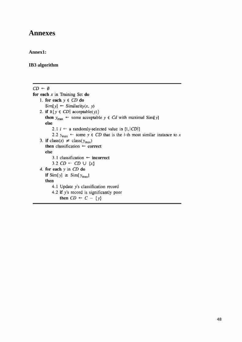
48

Annexes

Annex1: IB3 algorithm

49

Annex 2: The functioning of a simulated application As an example we took an application randomly and we explain over it. The choosen application is the one which simulate the Bluetooth: <application nom="Appli_Bluetooth" > <frequence min="360" max="8640" /> <duree min="1" max="30" /> <effets> <effet type="ajout_temporaire"> <target nom="memoireVive" /> <value valeur="39" /> </effet> <effet type="ajout_permanent"> <target nom= "memoirePhysique"/> <value valeur = "15" /> </effet> <effet type="ajout_periodique"> <target nom="batterie" /> <interval valeur = "7" /> <value valeur="-1" /> </effet> </effets> </application> This application can be turned on with a frequency, expressed in minutes, between the 2 bounds set as follows: <frequence min="360" max="8640" /> and it remains opened, each time, a specific duration randomly selected from a duration interval <duree min="1" max="30" /> During its functioning the application can modify a batch of parameters. In the precedent example it increases the RAM memory with 39 ‰ and also the ROM memory by 15 MB. Furthermore, periodically the battery is decreased by 1 at each 7 minutes. Another way of modifying parameters is presented in the recharge application, when the value of the battery is set at a fixed value as presented below: <application nom="Recharge" > <frequence min="1440" max="4320" /> <duree min="60" max="120" /> <effets> <effet type="setter_numeric"> <target nom="batterie" /> <value valeur="100" /> </effet> </effets> </application>

50

Annex 3: AQ21 running parameters Runs { Attribute_selection_method = promise Attribute_selection_threshold = 0.01 Ignore_attributes = typeplantage, age Random_seed = 100 Run_TF_crash { Mode = TF Consequent = [crash=true] Ambiguity = IncludeInMajority Trim = MostGen Maxstar = 5 Maxrule = 10 Display_events_covered = true Display_selectors_coverage = false Learn_rules_mode = multi_seed Number_of_seeds = 3 Negatives_percentage = 0.5 LEF_star { MinNegatives, 0 MaxPositives, 0 MaxNewPositives, 0 MinComplexity, 0 MaxSignificance, 0 MinCost, 0 MinNumSelectors, 0 } LEF_partial_star { MinNegatives, 0 MaxPositives, 0 MaxNewPositives, 0 MinComplexity, 0 MaxSignificance, 0 MinCost, 0 MinNumSelectors, 0 } LEF_sort { MinNumSelectors, 0 MinNegatives, 0 MaxPositives, 0 MaxNewPositives, 0 MinComplexity, 0 MaxSignificance, 0 MinCost, 0 } LEF_trunc { MinNegatives, 0 MaxPositives, 0 MaxNewPositives, 0 MinComplexity, 0 MaxSignificance, 0 MinCost, 0 MinNumSelectors, 0 } } }