incremental and multi-feature tensor subspace learning applied for background modeling and...
TRANSCRIPT
Incremental and Multi-feature Tensor Subspace Learning applied for Background Modeling and Subtraction
Andrews SobralPh.D. Student, Computer Vision
Lab. L3I – Univ. de La Rochelle, France

Summary
▪ Context
▪ Introduction to tensors
▪ Tensor decomposition methods
▪ Incremental tensor learning
▪ Incremental SVD
▪ Related Works
▪ Proposed method
▪ Conclusions
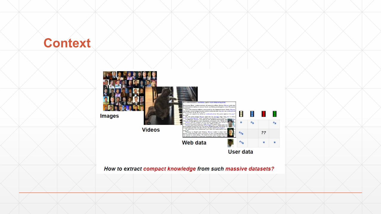
Context

Background Subtraction
Initialize Background
Modelframe model
ForegroundDetection
Background Model
Maintenance
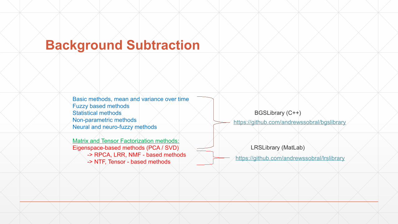
Background Subtraction
Basic methods, mean and variance over timeFuzzy based methodsStatistical methods Non-parametric methodsNeural and neuro-fuzzy methods
Matrix and Tensor Factorization methods:Eigenspace-based methods (PCA / SVD)
-> RPCA, LRR, NMF - based methods-> NTF, Tensor - based methods
https://github.com/andrewssobral/bgslibrary
LRSLibrary (MatLab)
BGSLibrary (C++)
https://github.com/andrewssobral/lrslibrary

Introduction to tensors

Background Subtraction
Initialize Background
Modelframe model
ForegroundDetection
Background Model
Maintenance

Introduction to tensors
▪ Tensors are simply mathematical objects that can be used to describe physical properties. In fact tensors are merely a generalization of scalars, vectors and matrices; a scalar is a zero rank tensor, a vector is a first rank tensor and a matrix is the second rank tensor.

Introduction to tensors
▪ Subarrays, tubes and slices of a 3rd order tensor.

Introduction to tensors
▪ Matricization of a 3rd order tensor.

110
1928
3746 51
19
1725
3341
48
1
9
17
25
33
41
48
kji
110
1928
3746 51
19
1725
3341
48
1
9
17
25
33
41
48
kj
i
110
1928
3746 51
19
1725
3341
48
1
9
17
25
33
41
48
kj
i
110
1928
3746 51
19
1725
3341
48
1
9
17
25
33
41
48
kj
i
110
1928
3746 51
19
1725
3341
48
1
9
17
25
33
41
48
kj
i
Frontal Vertical Horizontal
Horizontal, vertical and frontal slices from a 3rd order tensor
Introduction to tensors
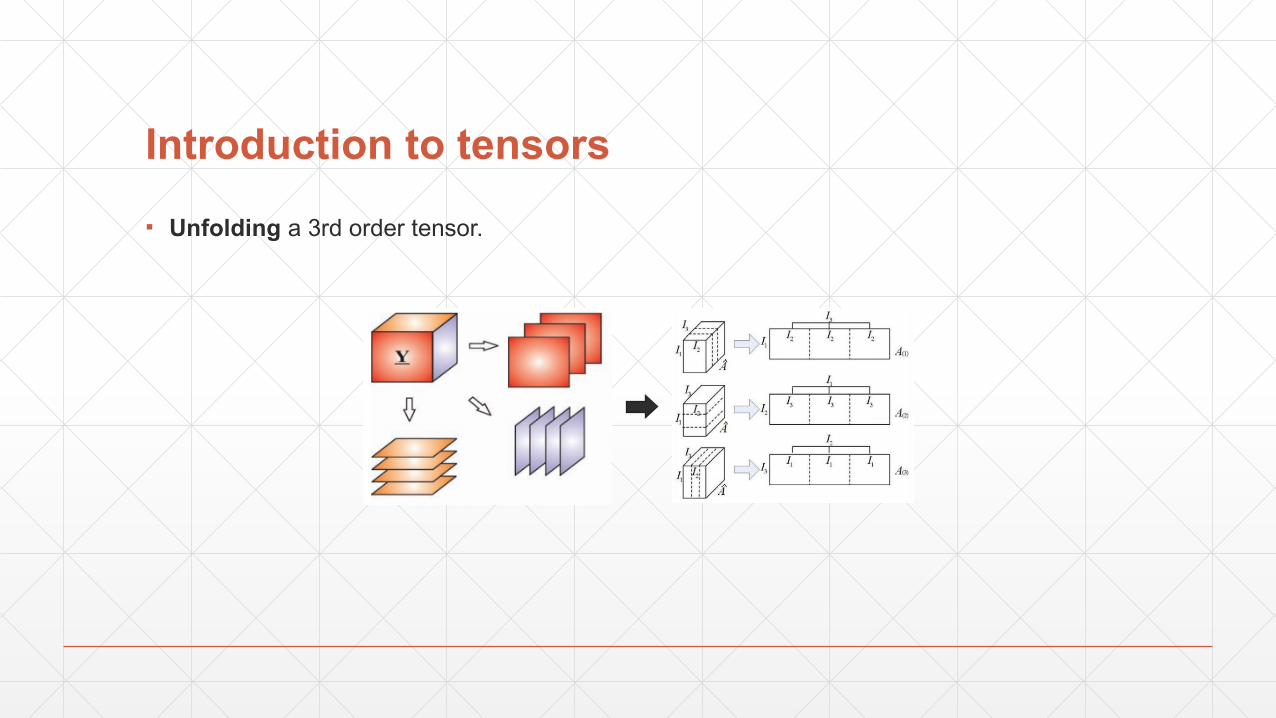
▪ Unfolding a 3rd order tensor.

Introduction to tensors
▪ Tensor transposition
▪ While there is only one way transpose a matrix there are an exponential number of ways to transpose an order-n tensor.
▪ The 3rd order case:

Tensor decomposition methods

Tensor decomposition methods
▪ Approaches:
▪ Tucker / HOSVD
▪ CANDECOMP-PARAFAC (CP)
▪ Hierarchical Tucker (HT)
▪ Tensor-Train decomposition (TT)
▪ NTF (Non-negative Tensor Factorization)
▪ NTD (Non-negative Tucker Decomposition)
▪ NCP (Non-negative CP Decomposition)
References:Tensor Decompositions and Applications (Kolda and Bader, 2008)


Tucker / HoSVD

CP
▪ The CP model is a special case of the Tucker model, where the core tensor is superdiagonal and the number of components in the factor matrices is the same.
Solving by ALS (alternating least squares) framework


Tensor decomposition methods
▪ Softwares
▪ There are several MATLAB toolboxes available for dealing with tensors in CP and Tucker decomposition, including the Tensor Toolbox, the N-way toolbox, the PLS Toolbox, and the Tensorlab. The TT-Toolbox provides MATLAB classes covering tensors in TT and QTT decomposition, as well as linear operators. There is also a Python implementation of the TT-toolbox called ttpy. The htucker toolbox provides a MATLAB class representing a tensor in HT decomposition.

Incremental tensor learning

Incremental SVD

Singular Value Decomposition
▪ Formally, the singular value decomposition of an m×n real or complex matrix M is a factorization of the form:
▪ where U is a m×m real or complex unitary matrix, Σ is an m×n rectangular diagonal matrix with nonnegative real numbers on the diagonal, and V* (the conjugate transpose of V, or simply the transpose of V if V is real) is an n×n real or complex unitary matrix. The diagonal entries Σi,i of Σ are known as the singular values of M. The m columns of U and the n columns of V are called the left-singular vectors and right-singular vectors of M, respectively.

-3 -2 -1 0 1 2 3-8
-6
-4
-2
0
2
4
6
8
10X Z
-3 -2 -1 0 1 2 3-8
-6
-4
-2
0
2
4
6
8
10Y Z Z
10 20 30 40
5
10
15
20
25
30
35
40
45
-8
-6
-4
-2
0
2
4
6
-4-2
02
4
-4
-2
0
2
4-10
-5
0
5
10
ORIGINAL
-4-2
02
4
-4
-2
0
2
4-10
-5
0
5
10
Z = 1
-4-2
02
4
-4
-2
0
2
4-10
-5
0
5
10
Z = 1 + 2

Incremental SVD
▪ Problem:
▪ The matrix factorization step in SVD is computationally very expensive.
▪ Solution:
▪ Have a small pre-computed SVD model, and build upon this model incrementally using inexpensive techniques.
▪ Businger (1970) and Bunch and Nielsen (1978) are the first authors who have proposed to update SVD sequentially with the arrival of more samples, i.e. appending/removing a row/column.
▪ Subsequently various approaches have been proposed to update the SVD more efficiently and supporting new operations.
References:Businger, P.A. Updating a singular value decomposition. 1970Bunch, J.R.; Nielsen, C.P. Updating the singular value decomposition. 1978

Incremental SVD
F(t) F(t+1) F(t+2) F(t+3) F(t+4) F(t+5)
[U, S, V] = SVD( [ F(t), …, F(t+2) ] ) [U’, S’, V’] = iSVD([F(t+3), …, F(t+5)], [U,S,V])
F(t) F(t+1) F(t+2) F(t+3) F(t+4) F(t+5)
[U, S, V] = SVD( [ F(t), …, F(t+1) ] ) [U’, S’, V’] = iSVD([F(t+1), …, F(t+3)], [U,S,V])
F(t) F(t+1) F(t+2) F(t+3) F(t+4) F(t+5)
[U, S, V] = SVD( [ F(t), …, F(t+2) ] ) [U’, S’, V’] = iSVD([F(t+1), …, F(t+3)], [U,S,V])
F(t) F(t+1) F(t+2) F(t+3) F(t+4) F(t+5)
[U, S, V] = SVD( [ F(t), …, F(t+1) ] ) [U’, S’, V’] = iSVD([F(t+1), …, F(t+3)], [U,S,V])

Incremental SVD
▪ Updating operation proposed by Sarwar et al. (2002):
References:Incremental Singular Value Decomposition Algorithms for Highly Scalable Recommender Systems (Sarwar et al., 2002)

Incremental SVD
▪ Operations proposed by Matthew Brand (2006):
References:Fast low-rank modifications of the thin singular value decomposition (Matthew Brand, 2006)

Incremental SVD
▪ Operations proposed by Melenchon and Martinez (2007):
References:Efficiently Downdating, Composing and Splitting Singular Value Decompositions Preserving the Mean Information (Melenchón and Martínez, 2007)

Incremental SVD algorithms in Matlab
By Christopher Baker (Baker et al., 2012)http://www.math.fsu.edu/~cbaker/IncPACK/[Up,Sp,Vp] = SEQKL(A,k,t,[U S V])Original version only supports the Updating operationAdded exponential forgetting factor to support Downdating operation
By David Ross (Ross et al., 2007)http://www.cs.toronto.edu/~dross/ivt/[U, D, mu, n] = sklm(data, U0, D0, mu0, n0, ff, K)Supports mean-update, updating and downdating
By David Wingate (Matthew Brand, 2006)http://web.mit.edu/~wingated/www/index.html[Up,Sp,Vp] = svd_update(U,S,V,A,B,force_orth)update the SVD to be [X + A'*B]=Up*Sp*Vp' (a general matrix update).
[Up,Sp,Vp] = addblock_svd_update(U,S,V,A,force_orth)update the SVD to be [X A] = Up*Sp*Vp' (add columns [ie, new data points])
size of Vp increasesA must be square matrix
[Up,Sp,Vp] = rank_one_svd_update(U,S,V,a,b,force_orth)update the SVD to be [X + a*b'] = Up*Sp*Vp' (that is, a general rank-one update. This can be used to add columns, zero columns, change columns, recenter the matrix, etc. ).

Incremental tensor learning

Incremental tensor learning
▪ Proposed methods by Sun et al. (2008)
▪ Dynamic Tensor Analysis (DTA)
▪ Streaming Tensor Analysis (STA)
▪ Window-based Tensor Analysis (WTA)
References:Incremental tensor analysis: Theory and applications (Sun et al, 2008)
Incremental tensor learning
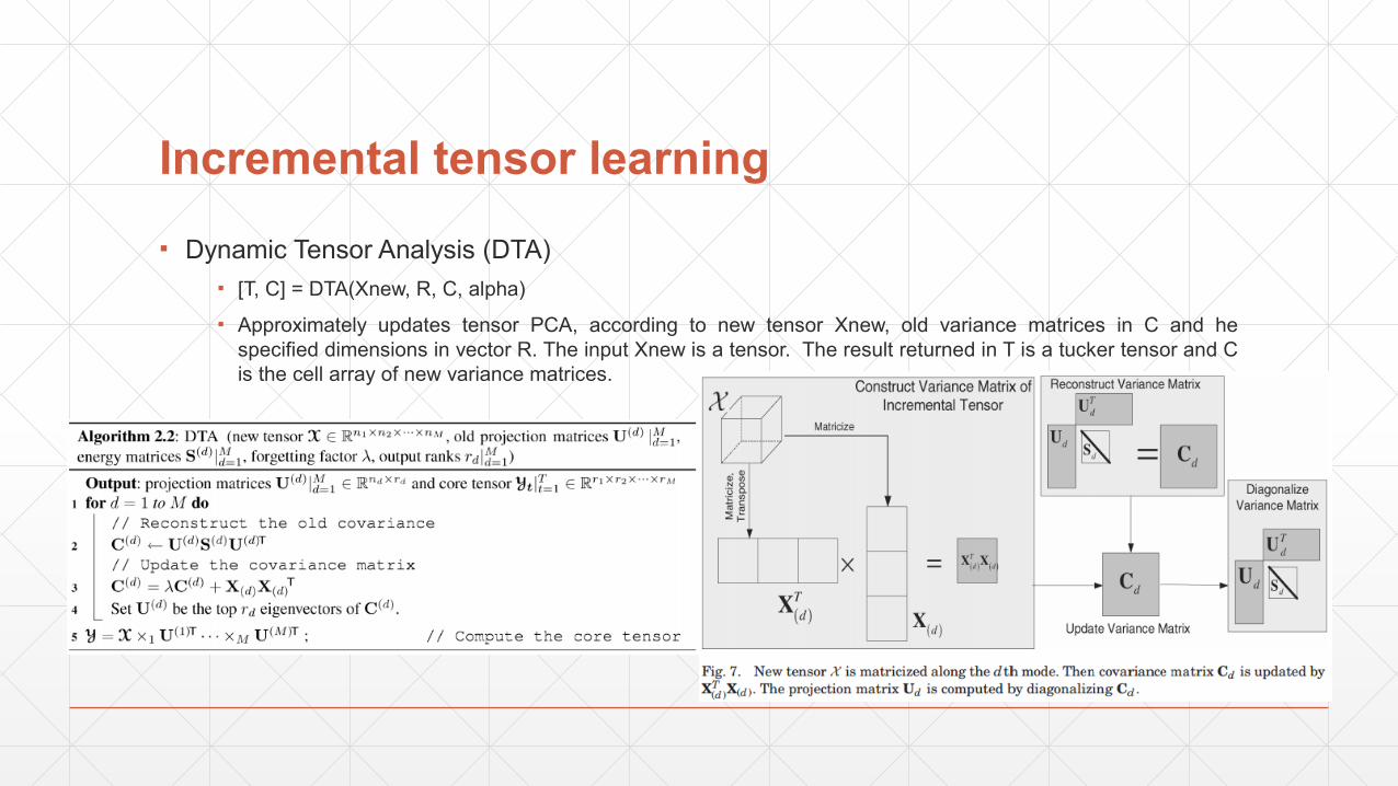
▪ Dynamic Tensor Analysis (DTA)▪ [T, C] = DTA(Xnew, R, C, alpha)
▪ Approximately updates tensor PCA, according to new tensor Xnew, old variance matrices in C and he specified dimensions in vector R. The input Xnew is a tensor. The result returned in T is a tucker tensor and C is the cell array of new variance matrices.

Incremental tensor learning
▪ Streaming Tensor Analysis (STA)▪ [Tnew, S] = STA(Xnew, R, T, alpha, samplingPercent)
▪ Approximately updates tensor PCA, according to new tensor Xnew, old tucker decomposition T and he specified dimensions in vector R. The input Xnew is a tensor or sptensor. The result returned in T is a new tucker tensor for Xnew, S has the energy vector along each mode.

Incremental tensor learning
▪ Window-based Tensor Analysis (WTA)▪ [T, C] = WTA(Xnew, R, Xold, overlap, type, C)
▪ Compute window-based tensor decomposition, according to Xnew (Xold) the new (old) tensor window, overlap is the number of overlapping tensors and C variance matrices except for the time mode of previous tensor window and the specified dimensions in vector R, type can be 'tucker' (default) or 'parafac'. The input Xnew (Xold) is a tensor,sptensor, where the first mode is time. The result returned in T is a tucker or kruskal tensor depending on type and C is the cell array of new variance matrices.

Incremental tensor learning
▪ Proposed methods by Hu et al. (2011)
▪ Incremental rank-(R1,R2,R3) tensor-based subspace learning
▪ IRTSA-GBM (grayscale)
▪ IRTSA-CBM (color)
References:Incremental Tensor Subspace Learning and Its Applications to Foreground Segmentation and Tracking (Hu et al., 2011)
Apply iSVD SKLM
(Ross et al., 2007)

Incremental tensor learning
▪ IRTSA architecture

Incremental rank-(R1,R2,R3) tensor-based subspace learning (Hu et al., 2011)
streaming video data
Background Modeling
Exponential moving average
LK
J(t+1)
new sub-frame
tensor
Â(t)
sub-tensor
APPLY STANDARD RANK-R SVDUNFOLDING MODE-1,2,3
Set of N background images
For first N frames
low-rank sub-tensor
model
B(t+1)
New backgroundsub-frame
Â(t+1)
B(t+1)
drop last frame
APPLY INCREMENTAL SVD UNFOLDING MODE-1,2,3
updated sub-tensor
foreground mask
For the next frames
For the next background sub-frame
Â(t+1)
updated sub-tensor
UPDATE
SKLM (Ross et al., 2007)
{bg|fg} = P( J[t+1] | U[1], U[2], V[3] )
Foreground Detection
Background ModelInitialization
Background ModelMaintenance

Proposed method

Proposed method
Performs feature extraction in the sliding block
Build or update the tensor model
Store the last N frames in a sliding block
streaming video data
Performs the iHoSVD to build or update the low-rank model
foreground mask
Performs the Foreground Detection
low-rank model
values
pixels
features
remove the last frame
from sliding block
add first frame coming from video stream
…
(a) (b) (c) (d) (e)

Proposed method
▪ Sliding block
remove the last frame from sliding block
add first frame coming from video stream

Proposed method
▪ Building Tensor Model
▪ A total of 8 features are extracted:
▪ 1) red channel,
▪ 2) green channel,
▪ 3) blue channel,
▪ 4) gray-scale,
▪ 5) local binary patterns (LBP),
▪ 6) spatial gradients in horizontal direction,
▪ 7) spatial gradients in vertical direction, and
▪ 8) spatial gradients magnitude. values
pixels
features
tensor model
…

Proposed method
▪ Incremental Higher-order Singular Value Decomposition
Fixed parameters:• r1 = 1• r2 = 8• r3 = 2• t1 = t2 = t3 = 0.01
It creates a low-rank tensor model Lt with the dominant singular subspaces of the tensor model Tt.

Proposed method
▪ Foreground detection
For each new frame a weighted combination of similarity measures is performed.
- Feature’s set extracted from input frame. - Feature’s set extracted from low-rank model.
- Similarity measure for the feature n. - Weighted combination of similarity measures.
The weights are chosen empirically:w1 = w2 = w3 = w6 = w7 = w8 = 0.125, w_4 = 0.225, w_5 = 0.025
Threshold t = 0.5

Proposed method
▪ Architecture
Feature Extraction+
iHoSVD
Initialize Background Model
frame modelForegroundDetection
Background Model Maintenance
Low Rank Tensor Model
Weighted combination of
similarity measures
x1
x3
x3
w1
w2
w3
yΣ ⁄

Proposed method
▪ Experimental results on BMC data set

Proposed method
▪ Experimental results on BMC data set

Proposed method
▪ Experimental results on BMC data set
Conclusions
▪ Experimental results shows that the proposed method achieves interesting results for background subtraction task.
▪ However, additional features can be added, enabling a more robust model of the background scene.
▪ In addition, the proposed foreground detection approach can be changed to automatically selects the best features allowing an accurate foreground detection.
▪ Further research consists to improve the speed of low-rank decomposition for real-time applications.
▪ Additional supports for dynamic backgrounds might be interesting for real and complex scenes.