incremental online learning in high...
TRANSCRIPT

Incremental Online Learning in High Dimensions
Sethu Vijayakumar, Aaron D’Souza & Stefan SchaalDepartment of Computer Science
University of Southern California, Los Angeles, CA 90089-2520,USA.sethu,adsouza,[email protected]
June 6, 2005
Abstract
Locally weighted projection regression (LWPR) is a new algorithm for incremental nonlinear func-tion approximation in high dimensional spaces with redundant and irrelevant input dimensions. Atits core, it employs nonparametric regression with locally linear models. In order to stay computa-tionally efficient and numerically robust, each local model performs the regression analysis with asmall number of univariate regressions in selected directions in input space in the spirit of partialleast squares regression. We discuss when and how local learning techniques can successfully workin high dimensional spaces and compare various techniques for local dimensionality reduction beforefinally deriving the LWPR algorithm. The properties of LWPR are that it i) learns rapidly withsecond order learning methods based on incremental training, ii) uses statistically sound stochasticleave-one-out cross validation for learning without the need to memorize training data, iii) adjustsits weighting kernels based only on local information in order to minimize the danger of negativeinterference of incremental learning, iv) has a computational complexity that is linear in the num-ber of inputs, and v) can deal with a large number of - possibly redundant - inputs, as shown invarious empirical evaluations with up to 50 dimensional data sets. For a probabilistic interpreta-tion, predictive variance and confidence intervals are derived. To our knowledge, LWPR is the firsttruly incremental spatially localized learning method that can successfully and efficiently operatein very high dimensional spaces.
1 Introduction
Despite the recent progress in statistical learning, nonlinear function approximation with high di-mensional input data remains a nontrivial problem, especially in incremental and real-time formula-tions. There is, however, an increasing number of problem domains where both these properties areimportant. Examples include the on-line modeling of dynamic processes observed by visual surveil-lance, user modeling for advanced computer interfaces and game playing, and the learning of valuefunctions, policies, and models for learning control, particularly in the context of high-dimensionalmovement systems like humans or humanoid robots. An ideal algorithm for such tasks needs toavoid potential numerical problems from redundancy in the input data, eliminate irrelevant inputdimensions, keep the computational complexity of learning updates low while remaining data effi-cient, allow for online incremental learning, and, of course, achieve accurate function approximationand adequate generalization.
When looking for a learning framework to address these goals, one can identify two broad classesof function approximation methods: (i) methods which fit non-linear functions globally, typicallyby input space expansions with predefined and/or parametrized basis functions and subsequent
1

linear combinations of the expanded inputs, and (ii) methods which fit non-linear functions lo-cally, usually by using spatially localized simple (e.g., low order polynomial) models in the originalinput space and automatically adjusting the complexity (e.g., number of local models and theirlocality) to accurately account for the nonlinearities and distributions of the target function. Inter-estingly, the current trends in statistical learning have concentrated on methods that fall primarilyin the first class of global nonlinear function approximators, for example, Gaussian Process Regres-sion(GPR)(Williams & Rasmussen, 1996), Support Vector Machine Regression(SVMR)(Smola &Scholkopf, 1998) and Variational Bayes for mixture models1(VBM) (Ghahramani & Beal, 2000).In spite of the solid theoretical foundations that these approaches possess in terms of generalizationand convergence, they are not necessarily the most suitable for on-line learning in high-dimensionalspaces. First, they require an a priori determination of the right modeling biases. For instance,in the case of GPR and SVMR, these biases involve selecting the right function space in terms ofthe choice of basis or kernel functions(Vijayakumar & Ogawa, 1999), and in VBM the biases areconcerned with the the right number of latent variables and proper initialization 2. Second, allthese recent function approximator methods were developed primarily for batch data analysis andare not easily and/or efficiently adjusted for incrementally arriving data. For instance, in SVMR,adding a new data point can drastically change the outcome of the global optimization problem interms of which data points actually become support vectors, such that all (or a carefully selectedsubset) of data has to be kept in memory for re-evaluation. Thus, adding a new data point inSVMR is computationally rather expensive, a property that is also shared by GPR. VBM suffersfrom similar problems due to the need of storing and re-evaluating data when adding new mixturecomponents (Ueda & Hinton, 2000). In general, it seems that most suggested Bayesian learningalgorithms are computationally too expensive for real-time learning because they tend to representthe complete joint distribution of the data, albeit as a conditionally independent factored repre-sentation. As a last point, incremental approximation of functions with global methods is proneto lead to negative interference when input distributions change (Schaal & Atkeson, 1998) – suchchanges are, however, a typical scenario in many on-line learning tasks.
In contrast to the global learning methods described above, function approximation with spa-tially localized models are rather well suited for incremental and real-time learning, particularlyin the framework of nonparametric regression (Atkeson, Moore, & Schaal, 1997). Nonparamet-ric 3 methods are very useful when there is limited knowledge about the model complexity suchthat the model resources need to be increased in a purely incremental and data driven fashion, asdemonstrated in previous work (Schaal & Atkeson, 1998). However, since these techniques allocateresources to cover the input space in a localized fashion, in general, with an increasing number ofinput dimensions, they encounter an exponential explosion in the number of local models requiredfor accurate approximation, ofter referred to as the ‘curse of dimensionality’ (Scott, 1992). Hence,at the outset, high-dimensional function approximation seems to be computationally infeasible forlocal nonparametric learning.
Nonparametric learning in high dimensional spaces with global methods, however, has beenemployed successfully by using techniques of projection regression (PR). PR copes with high di-mensional inputs by decomposing multivariate regressions into a superposition of single variateregressions along a few selected projections in input space. The major difficulty of PR lies in theselection of efficient projections, i.e., how to achieve the best fitting result with as few univariate
1Mixture models are actually somehow in between global and local function approximators since they use local modelfitting but employ a global optimization criterion.
2It must be noted that there has been some recent work(Scholkopf & Smola, 1999) that have started to look at modelselection for SVMs and GPRs and automatic determination of number of latent models for VBM (Ghahramani & Beal,2000)
3It should be noted that “nonparametric regression” does not mean that there are no parameters in the algorithm,but rather that the underlying distributions of a learning problem cannot be indexed with a finite number of parameters.Thus, the number of parameters in nonparametric regression usually grows with the number of training data. GPR andSVMR are also nonparametric algorithms, just that they fall in the class of “global” methods as described above.
2

regressions as possible. Among the best known PR algorithms are projection pursuit regression(Friedman & Stutzle, 1981), and its generalization in form of Generalized Additive Models (Hastie &Tibshirani, 1990). Sigmoidal neural networks can equally be conceived of as a method of projectionregression, in particular when new projections are added sequentially, e.g., as in Cascade Correlation(Fahlman & Lebiere, 1990).
In this paper we will suggest a method of extending the beneficial properties of local nonpara-metric learning to high dimensional function approximation problems. The prerequisite of ourapproach is that the high dimensional learning problems we address have locally low dimensionaldistributions, an assumption that holds for a large class of real world data (see below). If distri-butions are locally low dimensional, the allocation of local models can be restricted to these thindistributions, and only a tiny part of the entire high dimensional space needs to be filled withlocal models. Thus, the curse of dimensionality of spatially localized model fitting can be avoided.Under these circumstances, an alternative method of projection regression can be derived, focusingon finding efficient local projections. Local projections can be used to accomplish local functionapproximation in the neighborhood of a given query point with traditional local nonparametricapproaches, thus inheriting most of the statistical properties from the well established methodsof locally weighted learning and nonparametric regression (Hastie & Loader, 1993; Atkeson et al.,1997). As this paper will demonstrate, the resulting learning algorithm combines the fast, efficientand incremental capabilities of the non-parametric techniques while alleviating the problems faceddue to high dimensional input domains through local projections.
In the following sections, we will first motivate why many high dimensional learning problemshave locally low dimensional data distributions such that the prerequisites of our local learningsystem are justified. Second, we will address the question of how to find good local projectionsby looking into various schemes for performing dimensionality reduction for regression, includingprincipal component regression, factor analysis, partial least squares regression, and covariance pro-jection regression – a novel method that generalizes principal component regression towards partialleast squares regression. Empirical evaluations will highlight the pros and cons of the differentmethods. Finally, we will embed the most efficient and robust of these projection algorithms inan incremental nonlinear function approximator (Vijayakumar & Schaal, 1998) capable of auto-matically adjusting the model complexity in a purely data driven fashion. In several evaluations- both on synthetic and real world data - the resulting incremental learning system demonstrateshigh accuracy for function fitting in very high dimensional spaces, robustness towards irrelevantand redundant inputs, as well as low computational complexity. Comparisons will prove the com-petitiveness with other state-of-the-art learning systems.
2 Evidence for low dimensional distributions
The development of our learning system in the next sections relies on the assumption that highdimensional data sets have locally low dimensional distributions, an assumption that requires someclarification. Across domains like vision, speech, motor control, climate patterns, human genedistributions, and a range of other physical and biological sciences, various researchers have reportedevidence that corroborate the fact that the true intrinsic dimensionality of high dimensional datais often very low (Tenenbaum & Langford, 2000; Roweis & Saul, 2000; Vlassis, 2002). We interpretthese findings as evidence that the physical world has a significant amount of coherent structure thatexpresses itself in terms of strong correlations between different variables that describe the stateof the world at a particular moment in time. For instance, in computer vision it is quite obviousthat neighboring pixels of an image of a natural scene have redundant information. Moreover,the probability distribution of natural scenes in general has been found to be highly structuredsuch that it lends itself to a sparse encoding in terms of set of basis functions (Olshausen &Field, 1996; Bell & Sejnowski, 1997). Another example comes from our own research on humanmotor control. Despite that humans can accomplish movement tasks in almost arbitrary ways –
3

0
0.1
0.2
0.3
0.4
0.5
0.6
0.7
0.8
0.9
1
0 10 20 30 40 50
Cum
ulat
ive
varia
nce
No. of retained dimensions7.78
/ /
105/ /
(a)
1 11 21 31 410
0.05
0.1
0.15
0.2
0.25
Pro
babi
lity
Dimensionality
(b)
Figure 1: Dimensionality Analysis - (a) The cumulative variance accounted versus the local dimension-ality (avearged across all mixture models) (b) The distribution of the effective dimensionality acrossall mixture models
thus possibly generating arbitrary distributions of the variables that describe their movements –behavioral research has discovered a tremendous amount of regularity within and across individuals(Kawato, 1999; Schaal & Sternad, 2001). These regularities lead to locally low dimensional datadistribution, as illustrated in the example in Fig. 1. In this analysis(D’Souza & Schaal, 2001), weassessed the intrinsic dimensionality of data collected from full body movement of several humansubjects, collected with a special full-body exoskeleton that recorded simultaneously 35 degrees-of-freedom of the joint angular movement of the subjects at 100hz sampling frequency. Subjectsperformed a variety of daily-life tasks (e.g., walking, object manipulation, reaching, etc.) untilabout a gigabyte of data was accumulated. Our analysis examined the local dimensionality ofthe joint distribution of positions, velocities, and accelerations of the collected data, i.e., a 105dimensional data set, as would be needed as inputs to learn an inverse dynamics model for motorcontrol (Kawato, 1999). As an analysis tool, we employed a variational Bayesian mixture of factoranalyzers that automatically estimated the required number of mixture components (Ghahramani &Beal, 2000). As demonstrated in Fig. 1(a), the local dimensionality was around 5 to 8 dimensions,computed based on the average number of significant latent variables per mixture component. Fig.1(b) shows the distribution of the effective dimensionality across all mixture models.
In summary, the results from our analysis and other sources in the literature show that there is alarge class of high dimensional problems that can be treated locally in much lower dimensions if onecan determine appropriate regions of locality and the local projections that model the correspondinglow dimensional distributions. As a caveat, however, it may happen that such low dimensionaldistributions are embedded in additional dimensions that are irrelevant for the problem at handbut have considerable variance. In the context of regression, it will thus be important to only modelthose local dimensions that carry information that is important for the regression and eliminate allother dimensions, i.e., to perform local dimensionality reduction with regression in mind and notjust based on input or joint input-output distributions, as discussed in the next section.
3 Local dimensionality reduction
Assuming that data is characterized by locally low dimensional distributions, efficient algorithmsare needed to exploit this property. For this purpose, we will focus on locally weighted learning(LWL) methods (Atkeson et al., 1997) because they allow us to adapt a variety of linear dimension-ality reduction techniques for the purpose of nonlinear function approximation (see Section 4) andbecause they are easily modified for incremental learning. LWL-related methods have also foundwidespread application in mixture models (Jordan & Jacobs, 1994; Xu, Jordan, & Hinton, 1995;Ghahramani & Beal, 2000) such that the results of this section can contribute to this field, too.
4

In pursuit of the question of what is the “right” method to perform local dimensionality reduc-tion for regression, the following sections will compare several candidate techniques theoreticallyand empirically. In particular, we will derive and investigate locally weighted versions of prin-cipal component regression (LWPCR), joint data principal component analysis (LWPCA), factoranalysis (LWFA) and partial least squares (LWPLS). In addition, we will develop a novel familyof projection regression technique, named covariant projection regression (LWCPR). In the nextsections, we will first outline the algorithms of each of these methods before conducting empiricalevaluations to test their robustness in situations where their data generating model is violated.
3.1 The locally weighted regression model
The learning problems considered here assume the standard regression model:
y = f(x) + ε.
where x denotes the d-dimensional input vector, y the (for simplicity) scalar output, and ε a mean-zero random noise term. When only a local subset of data in the vicinity of a point xc is consideredand the locality is chosen appropriately, a low order polynomial can be employed to model this localsubset. Due to a favorable compromise between computational complexity and quality of functionapproximation (Hastie & Loader, 1993), we choose linear models
y = βT x + ε.
A measure of locality for each data point, the weight wi, is computed from a Gaussian kernel:
wi = exp(−0.5(xi − xc)T D(xi − xc)), and W ≡ diagw1, . . . , wM (1)
where D is a positive semi-definite distance metric which determines the size and shape of theneighborhood contributing to the local model (Atkeson et al., 1997). The weights wi will enterall following algorithms to assure spatial localization in input space. In particular, zero meanprerequisites of several algorithms is ensured by subtracting the weighted mean x or y from thedata, where
x =M∑
i=1
wixi/
M∑
i=1
wi, and y =M∑
i=1
wiyi/
M∑
i=1
wi, (2)
and M denotes the number of data points. For simplicity, and without loss of generality, we willthus assume in the derivations in the next sections that all input and output data have a weightedmean of zero with respect to a particular weighting kernel. The input data is summarized in therows of the matrix X=[x1 x2 ...xM ]T , the corresponding outputs are the coefficients of the vectory, and the corresponding weights, determined from eq.(1), are in the diagonal matrix W. In somecases, we need the joint input and output data, denoted as Z=[z1 z2...zM ]T = [X y].
3.2 Locally Weighted Factor Analysis (LWFA)
Factor analysis(Everitt, 1984) is a density estimation technique that assumes that the observed dataz were actually generated from a lower dimensional process, characterized by k latent or hiddenvariables v that are all independently distributed with mean zero and unit variance. The observedvariables are generated form the latent variables through the transformation matrix U and additivemean zero independent noise ε with diagonal covariance matrix Ω:
z = Uv + ε, (3)
where
z =[
xy
], ε =
[εx
εy
], EεεT = Ω, (4)
5

and E. denotes the expectation operator. If both v and ε are normally distributed, the parametersΩ and U can be obtained iteratively by the Expectation-Maximization algorithm (EM) (Rubin &Thayer, 1982).
Factor analysis can be adapted for linear regression problems by assuming that z was generatedwith
U = [Id β]T (5)v = x (6)
where β denotes the vector of regression coefficients of the linear model y = βT x and Id the d-dimensional identity matrix. For the standard regression model, εx would be zero, i.e. we considernoise contamination in the output only – for numerical reasons, however, some remaining varianceneeds to be permitted and we prefer to leave it to the EM algorithm to find the optimal values of thecovariance Ω. After calculating Ω and U with EM in joint data space as formulated in eq.(3), anestimate of β can be derived from the conditional probability p(y|x). Let us denote Z=[z1 z2...zM ]T
and V=[v1 v2...vM ]T . The locally weighted version (LWFA) of β can be obtained together withan estimate of the factors v from the joint weighted covariance matrix Ψ of z and v as
E[
yv
]|x =
[βT
B
]x = Ψ21Ψ−1
11 x, (7)
where
Ψ = [ZT VT ]W[
ZV
]/
M∑
i=1
wi =[
Ω + UUT UUT Id
]=
[Ψ11 Ψ12
Ψ21 Ψ22
], (8)
and B is a matrix of coefficients involved in estimating the factors v. Note that unless the noise εx
is zero, the estimated β is different from the true β as it tries to optimally average out the noisein the data. Thus, factor analysis can also be conceived of as a tool for linear regression with noisecontaminated inputs.
3.3 Principal Component Regression(LWPCR)
Although not optimal, a computationally efficient technique of dimensionality reduction for linearregression is the principal component regression (Massy, 1965; Vijayakumar & Schaal, 1998). Forlocally weighted principal component regression (LWPCR), let us represent the covariance matrixof the weighted input data, Clwpcr, as
Clwpcr =M∑
i=1
wixixTi /
M∑
i=1
wi (9)
and its eigenvalue decomposition in form of
Clwpcrci = λici (10)
where, λ1 > λ2 > .... The dimensionality reduction step in LWPCR projects the inputs onto thek largest principal components of Clwpcr by the transformation matrix U whose columns are theunit eigenvectors corresponding to the k largest eigenvalues of Clwpcr given by
U ≡ [c1 c2 ... ck]. (11)
The vector of regression coefficients can then be calculated as
β = (UT XT WXU)−1UT XT Wy. (12)
6

Eq.(12) is inexpensive to evaluate since after projecting X with U, UT XT WXU becomes a diagonalmatrix that is can be inverted easily. Essentially, LWPCR performs univariate regressions alongorthogonal projection directions of the inputs space. A pseudocode implementation of the LWPCRis given in the Appendix A.
LWPCR assumes that the inputs have additive spherical noise, which includes the zero noisecase. Since, during dimensionality reduction, LWPCR does not take into account the output data,it is susceptible to ignoring input dimensions with low variance which nevertheless have importantcontribution to the regression output. Also, if the input data has non-spherical noise and irrelevantdimensions, LWPCR is prone to focus the regression on irrelevant projections.
3.4 Principal Component in Joint Space(LWPCA J)
An alternative way of determining the parameters in a reduced space employs locally weightedprincipal component analysis in the joint data space (LWPCA J). Let us denote the weightedcovariance matrix of the joint data Z = [Xy] as Clwpca, which is given by
Clwpca =M∑
i=1
wi(zi − z)(zi − z)T /
M∑
i=1
wi. (13)
Let the eigenvalue decomposition of Clwpca be given as
Clwpcaci = λici (14)
where, λ1 > λ2 > .... Let us define a dimensionality reduction transformation matrix U as
U ≡ [c1 c2 ... ck+1], (15)
which is the projection onto the space spanned by the k+1 largest principal components of the jointdata. Noting that the eigenvectors in U are unit length, the matrix inversion theorem (Horn &Johnson, 1994) provides a means to derive an efficient estimate of β as
β = Ux(UTy −UT
y (UyUTy − Ip)−1UyUT
y ), (16)
where U is decomposed into Ux and Uy as
U =[
Ux
Uy
], (17)
and p is the dimensionality of the outputs. In our one dimensional output case, p = 1 and Uy
is just a (1 × k)-dimensional row vector, and the evaluation of eq.(16) does not require a matrixinversion anymore but rather only a division. If we assume normal distributions in all variables as inLWFA, LWPCA J is the special case of LWFA where the noise covariance is spherical, i.e., the samemagnitude of noise in all observables. Under these circumstances, the subspaces spanned by U inboth methods will be the same (Tipping & Bishop, 1999). However, the regression coefficients ofLWPCA J will be different from those of LWFA unless the noise level is zero, as LWFA optimizes thecoefficients by taking into account the noise in the data (refer eq.(7)). Thus, for normal distributionsand a correct guess of k, LWPCA J is always expected to perform worse than LWFA.
3.5 Partial Least Squares(LWPLS)
Partial least squares (PLS) (Wold, 1975; Frank, 1993), a technique extensively used in chemomet-rics, recursively computes orthogonal projections of the input data and performs single variableregressions along these projections on the residuals of the previous iteration step. Table 1 providesan outline of the PLS algorithm. The key ingredient in PLS is to use the direction of maximal
7

Table 1: Outline of Partial Least Squares (PLS) Regression Algorithm
1. Initialize: Xres = X, yres = y
2. for i = 1 to k do
(a) ui = XTresyres.
(b) βi = sTi yres/(sT
i si) where si = Xresui.
(c) yres = yres − siβi, Xres = Xres − sipiT where pi = XT
ressi/(sTi si).
correlation between the residual error and the input data as the projection direction at every re-gression step. Additionally, PLS regresses the inputs of the previous step against the projectedinputs s in order to ensure the orthogonality of all the projections u (Step 2c). Actually, thisadditional regression could be avoided by replacing p with u in Step 2c, similar to techniques usedin principal component analysis (Sanger, 1989). However, using this regression step leads to betterperformance of the algorithm as PLS chooses the most effective projections if the input data has aspherical distribution: in the spherical case, with only one projection, PLS will find the direction ofthe gradient and achieve optimal regression results. The regression step in 2c chooses the reducedinput data Xres such that the resulting data vectors have minimal norms and, hence, push thedistribution of Xres to become more spherical. An additional consequence of 2c is that all theprojections si become uncorrelated, i.e., sT
j si = 0 ∀i 6= j; a property which will be important inthe derivations below. Appendix A provides the modifications necessary for implementing a locallyweighted version (LWPLS) of the algorithm.
3.6 Covariant Projection Regression (LWCPR)
In this section, we introduce a new algorithm which has the flavor of both PCR and PLS. CovariantProjection Regression(CPR) transforms the input data by a (diagonal) weight matrix T
Xt = TX
with the goal to elongate the distribution in the direction of the gradient of the input/outputrelation of the data. Subsequently, the major principal component of this deformed distribution ischosen as the direction of a univariate regression. In contrast to PCR, this projection now reflectsnot only the influence of the input distribution but also that of the regression outputs. As inPLS, if the input distribution is spherical, CPR will obtain an optimal regression result with asingle univariate fit, irrespective of the actual input dimensionality. If the input distribution is notspherical, several CPR projection need to be cascaded, similar to PLS. Refer to Appendix A forthe implementation pseudocode.
CPR is actually a family of algorithms, depending on how the weights in T are chosen. Weconsider two such options:
Weighting scheme CPR1: T cpr1ii = 1
σXres( |yres,i|‖xres,i‖ )
p.
Weighting scheme CPR2: T cpr2ii = 1
‖xres,i‖ (|yres,i|‖xres,i‖ )
p.
Note that the subscript res above denotes that x and y may not be the original input and outputdata anymore but rather residuals from the previous projection.
CPR1 spheres the input data and then weights it by the “slope” of each data point, taken to thepower p (where p is an even number) for increasing the impact of the input/output relationships.CPR2 is a variant that, although a bit idiosyncratic, had the best average performance in practice:
8

CPR2 first maps the input data onto a unit-(hyper)sphere, and then stretches the distributionalong the direction of maximal slope, i.e., the regression direction – this method is fairly insensitiveto noise in the input data.
3.7 Monte Carlo evaluations for performance comparison
3.7.1 Methods
In order to evaluate the candidate algorithms empirically, mean zero linear data sets, consistingof 1000 training points and 2000 test points, with 5 input dimension and 1 output were generatedat random. The outputs were calculated from random linear coefficients, and Gaussian noise wasadded. Then, the input data were augmented with 5 additional dimensions containing only zerovalues and rotated and stretched to have random variances in all dimensions. For some test cases,5 more input dimensions with random (non-constant) values were added afterwards to explore theeffect of irrelevant inputs on the regression performance. Empirically, we determined p = 4 as agood choice for the CPR methods. Given that the datasets were perfectly linear, we omitted anylocal weighting of the data, i.e., wi = 1 for all data points.
The simulations considered the following permutations:
• Low noise4 (r2=0.99) and High noise (r2 = 0.9) in output data.
• With and without irrelevant (non-constant) input dimensions.
• With four different guesses for the dimensionality of the latent variable space, i.e., k = 1, 4, 5,or 6.
Each algorithm was run5 100 times on random data sets of each of the 16 combinations of testconditions. The nMSE results of all trials were averaged and are reported as “averaged nMSE”. Fig.2 shows the summary results. The best nMSE values possible under the chosen noise conditionsare nMSE=0.01 for the low noise cases and nMSE=0.1 for the high noise case.
3.7.2 Results
Using only one projection, i.e., k = 1, was intended to investigate how well each of the algorithmswould be suitable for insertion into a learning scheme that increases the number of projectionsincrementally. For such constructive learning, it is desirable that the first projection itself reducesthe mean squared error of the regression as much as possible. With respect to this criterion,Fig.2(a) demonstrates that LWFA and LWPCR perform rather bad, while LWPLS, LWCPR andLWPCA J achieve significantly better results. For LWFA, the reduced performance is most likelyto be attributed to overestimating the noise in the data, which subsequently adversely affects thedetermination of the regression parameters. For LWPCR, the performance disadvantage can beblamed on selecting the projection direction without taking the outputs into account. In contrast,the slightly heuristic determination of projection directions in LWPLS and LWCPR proves to berather powerful, as previously observed in numerous PLS papers (Frank, 1993).
In Fig.2(c), the number of factors equals the underlying dimensionality of the problem. Allalgorithms are essentially performing equally well in the case of no irrelevant dimensions, althoughLWPCA J shows some disadvantage due to its assumption of equal amounts of noise in both inputsand outputs. However, with five extra irrelevant inputs, i.e., a total number of 15 input dimensions
4Noise is parametrized by the coefficient of determination r2 of standard linear regression, defined as r2 = (σ2y −
σ2res)/σ2
y, where σ2res is the variance of the residual error and σ2
y is the variance of the outputs. We add noise scaledto the variance of the non-noise contaminated outputs y such that σ2
noise = cσ2y, where c = 1
r2−1. The best normalized
mean squared error (nMSE) achievable by a learning system under this noise level is 1 − r2, unless the system overfitsthe data.
5Except for LWFA, all methods can evaluate a data set in non-iterative calculations. LWFA was trained with EM formaximally 1000 iterations or until the log-likelihood increased less than 1.0e-10 in one iteration.
9

0
0.1
0.2
0.3
0.4
0.5
0
0.1
0.2
0.3
0.4
0.5
Ave
rage
nM
SE
on
test
dat
a
(d) Regression results with 6 factors (one too many)
LWFA LWPCA_J LWPCR LWPLS LWCPR1 LWCPR2
Low Noise High NoiseLow Noise &irrelevant dim.
High Noise &irrelevant dim.
0
0.1
0.2
0.3
0.4
0.5
0
0.1
0.2
0.3
0.4
0.5
Ave
rage
nM
SE
on
test
dat
a
(a) Regression results with one factor(projection)
0
0.1
0.2
0.3
0.4
0.5
0
0.1
0.2
0.3
0.4
0.5
Ave
rage
nM
SE
on
test
dat
a
(b) Regression results with 4 factors (one too few)
0
0.1
0.2
0.3
0.4
0.5
0
0.1
0.2
0.3
0.4
0.5
Ave
rage
nM
SE
on
test
dat
a
(c) Regression results with 5 factors (true # of factors)
Figure 2: Summary results of Monte Carlo experiments. The subplots show results for projectiondimensions 1, 4, 5 and 6. Each of the subplots has four additional conditions made of permutationsof: (i) low and high noise (ii) with and without irrelevant (non constant) inputs. Error bars areone standard deviation computed from 100 repetitions in each test condition. The best nMSE valuesachievable are 0.01 (for the low noise datasets) and 0.1 (for the high noise datasets).
10

with underlying latent space of 10 dimensions, LWFA and LWPCR also show significant degradationin performance. For LWPCR, this effect can again be attributed to its dimensionality reductionbased on only the inputs. For LWFA, it is important that the entire latent space is represented bythe factors, even if some of these variables are irrelevant for regression. Thus, the same effect asexplained for k = 1 accounts for LWFA’s reduced performance.
For the case of underestimating the number of necessary projections by one (Fig.2(b)), againLWPCR and LWFA show reduced performance for the same reasons as for k = 5 with irrelevantinputs. LWPLS and LWCPR do rather well with LWPLS having a slight lead in noisier situations.The advantage of LWPLS for situations with more noise is due to its method of projection selection:noise is averaged out in the correlation of inputs and outputs, while in LWCPR, noise can affect theselection of the projection direction as it is nonlinearly transformed by the exponent p. LWPCA Jranks third in this comparison.
Finally, for the case with one factor too many (Fig.2(d)), the pattern of k = 5 repeats itself.Thus, all methods show no significant degradation due to using too many projections. However, inpractice, we will be more interested in approximations with a smaller number of projections thanactually needed in order to save resources and reduce computational complexity.
We conclude that LWPLS and LWCPR outperform LWPCR, LWFA and LWPCA J by a sig-nificant margin when the learning data does not match the assumptions of the chosen algorithm.LWPCR tends to deteriorate due to performing dimensionality reduction without taking the regres-sion outputs into account, thus rejecting dimensions that have low variance but are neverthelessimportant for reducing the mean squared error. Although being theoretically the most appealing,LWFA turned out to be very sensitive to the selection of the correct number of factors, essentiallyrequiring that the entire latent space of the inputs is represented, no matter whether some of thesedimensions contribute to the regression or not. This property makes LWFA rather expensive forhigh dimensional problems and also less suitable for growing the number of projections incremen-tally. LWPCA J turned out to be a mediocre but on average, a robust method of dimensionalityreduction. In all situations, LWCPR and LWPLS performed equally good or better than any of theremaining algorithms. For low noise (r2 = 0.99), LWCPR has a marginal lead over LWPLS, espe-cially during the first projections. For high noise cases (r2 = 0.9), LWPLS has a slight advantage,due to its noise insensitive way of selecting projections. Among the LWCPR candidates, LWCPR2seems to outperform LWCPR1 in low noise cases, while this trend is reversed for high noise cases– the difference between the two algorithms is statistically insignificant.
In summary, both LWCPR and LWPLS perform very well and accomplish excellent regressionresults with relatively few projections since their choice of projection directions does not just try totake into account the input distribution but also the gradient of the data. In the next section, we willembed one of these algorithms in an incremental nonlinear function approximator to demonstrateits abilities for non-trivial function fitting problems.
4 Locally Weighted Projection Regression
For nonlinear function approximation, the core concept of our learning system – Locally WeightedProjection Regressionn (LWPR), is to find approximations by means of piecewise linear models(Atkeson et al., 1997). Learning involves automatically determining the appropriate number oflocal models K, the parameters βk of the hyperplane in each model, and also the region of validity,called receptive field (RF), parameterized as a distance metric Dk in a Gaussian kernel:
wk = exp(−12(x− ck)T Dk(x− ck)). (18)
11

Table 2: Legend of indexes and symbols used for LWPR
Notation AffectationM No. of training data pointsN Input dimensionality (i.e. dim. of x)k = (1 : K) Number of local modelsr = (1 : R) Number of local projections used by PLSxi, yiM
i=1 Training DataziM
i=1 Lower dimensional projection of input data xi(by PLS)zi,rR
r=1 Elements of projected inputX, Z Batch representations of input and projected dataw Weight or activation of data (x, y) with respect to
local model or receptive field(RF) center cW Weight matrix: W ≡ diagw1, . . . , wNWn Cumulative weights (after n data points) seen be local modelan
var,r Trace variable for incremental computation of r-th dimension ofvariable ′var′ after seeing n data points.
Given a query point x, every linear model calculates a prediction yk(x). The total output of thelearning system is the normalized weighted mean of all K linear models:
y =K∑
k=1
wkyk/
K∑
k=1
wk, (19)
also illustrated in Fig. 3. The centers ck of the RFs remain fixed in order to minimize negative inter-ference during incremental learning that could occur due to changing input distributions (Schaal &Atkeson, 1998). Local models are createdon an ‘as-needed’ basis as described in Section 4.2. Table2 provides a reference list of indices and symbols that are used consistently across the descriptionof the LWPR algorithm.
4.1 Learning with LWPR
Despite its appealing simplicity, the “piecewise linear modeling” approach becomes numericallybrittle and computationally too expensive in high dimensional input spaces when using ordinarylinear regression to determine the local model parameters (Schaal & Atkeson, 1998). Given theempirical observation (cf. Section 2) that high dimensional data often lie on locally low dimensionaldistributions, and given the algorithmic results in Section 3, we will thus use local projectionregression, i.e., LWPLS or LWCPR, within each local model to fit the hyperplane. As a significantcomputational advantage, we expect that far fewer projections than the actual number of inputdimensions are needed for accurate learning. For an incremental learning algorithm, we choseLWPLS for our nonlinear implementation as PLS is already well established in the literature andis more straightforward to convert to incremental updates (cf. (Vijayakumar & Schaal, 1998) foran incremental strategy for LWCPR). The next sections will describe the necessary modificationsof LWPLS for this implementation, embed the local regression into the LWL framework, explaina method of automatic distance metric adaptation, and finish with a complete nonlinear learningscheme, called locally weighted projection regression (LWPR).
12

Output
PLSui,k
x1
x2
x3
x4
xn
ytrainLearning Module Input
Dk
wk
yk^
Xreg
βi,k
Σ
y^
Weighted
Average
Receptive field
centered at ck
Inputs
Linear unit
Correlation Computation module
X input
Figure 3: Information processing unit of LWPR
4.1.1 Incremental computation of projections and local regression
For incremental learning, i.e., a scheme that does not explicitly store any training data, the sufficientstatistics of the learning algorithm need to be accumulated in appropriate variables. Table 3(Vijayakumar & Schaal, 2000) provides suitable incremental update rules. The variables azz,r,azres,r and axz,r are sufficient statistics that enable us to perform the univariate regressions instep 2c.1.2 and step 2c.2.2, similar to recursive least squares, i.e., a fast Newton-like incrementallearning technique. λ ∈ [0, 1] denotes a forgetting factor that allows exponential forgetting of olderdata in the sufficient statistics. Forgetting is necessary in incremental learning since a change ofsome learning parameters will affect a change in the sufficient statistics – such forgetting factorsare a standard technique in recursive system identification (Ljung & Soderstrom, 1986). It can beshown that the prediction error of step 2b corresponds to the leave-one-out cross validation errorof the current point after the regression parameters were updated with the data point - hence, it isdenoted by ecv.
In Table 3, for R = N , i.e. the same number of projections as the input dimensionality, the entireinput space would be spanned by the projections ur and the regression results would be identical tothat of ordinary linear regression(Wold, 1975). However, once again, we would like to emphasize theimportant properties of the local projection scheme. First, if all the input variables are statisticallyindependent and have equal variance6, PLS will find the optimal projection direction ur in roughlya single sweep through the training data – the optimal projection direction corresponds to thegradient of the local linearization parameters of the function to be approximated. Second, choosingthe projection direction from correlating the input and the output data in Step 2b.1 automatically
6It should be noted that we could insert one more preprocessing step in Table 3 that independently scales all inputsto unit variance – empirically, however, we did not notice a significant improvement of the algorithm, such that we omitthis step for the sake of simplicity.
13

Table 3: Incremental locally weighted PLS for one RF centered at c
1. Initialization: (# data points seen n = 0)x0
0 = 0, β00 = 0, W 0 = 0, u0
r = 0; r = 1 : R
2. Incorporating new data: Given training point (x, y)
2a. Compute activation and update the means1. w = exp(−1
2(x− c)TD(x− c)); Wn+1 = λWn + w
2. xn+10 = (λWnxn
0 + wx)/Wn+1; βn+10 = (λWnβn
0 + wy)/Wn+1
2b. Compute the current prediction errorxres,1 = x− xn+1
0 , y = βn+10
Repeat for r = 1 : R (# projections)1. zr = xT
res,runr /
√un
rTun
r
2. y ← y + βnr zr
3. xres,r+1 = xres,r − zrpnr
4. MSEn+1r = λMSEn
r + w (y − y)2
ecv = y − y
2c. Update the local modelres1 = y − βn+1
0
For r = 1 : R (# projections)2c.1 Update the local regression and compute residuals
1. an+1zz,r = λ an
zz,r + w z2r ; an+1
zres,r = λ anzres,r + w zr resr
2. βn+1r = an+1
zres,r/an+1zz,r
3. resr+1 = resr − zrβn+1r
4. an+1xz,r = λ an
xz,r + wxres,rzr
2c.2 Update the projection directions1. un+1
r = λ unr + wxres,r resr
2. pn+1r = an+1
xz,r/an+1zz,r
e = resr+1
3. Predicting with novel data (xq): Initialize: yq = β0,xq = xq − x0
Repeat for r = 1 : R
• yq ← yq + βrsr where sr = uTr xq
• xq ← xq − srpnr
Note: The subscript k referring to the k-th local model is omitted throughout this table since we arereferring to updates in one local model or RF
14

excludes irrelevant input dimensions. And third, there is no danger of numerical problems due toredundant input dimensions as the univariate regressions can easily be prevented from becomingsingular.
Given that we will adjust the distance metric to optimize the local model approximation (seenext section), it is also possible to perform LWPR with only one projection direction (denoted asLWPR-1). In this case, this distance metric will have to be adjusted to find the optimal receptivefield size for a local linearization as well as to make the locally weighted input distribution spherical.An appropriate learning rule of the distance metric can accomplish this adjustment, as explainedbelow. It should be noted that LWPR-1 is obtained from Table 3 by setting R = 1.
4.1.2 Adjusting the shape and size of receptive field
The distance metric D and hence, the locality of the receptive fields, can be learned for each localmodel individually by stochastic gradient descent in a penalized leave-one-out cross validation costfunction (Schaal & Atkeson, 1998):
J =1∑M
i=1 wi
M∑
i=1
wi(yi − yi,−i)2 +γ
N
N∑
i,j=1
D2ij (20)
where M denotes the number of data points in the training set. The first term of the cost functionis the mean leave-one-out cross validation error of the local model (indicated by the subscript i,−i)which ensures proper generalization (Schaal & Atkeson, 1998). The second term, the penalty term,makes sure that receptive fields cannot shrink indefinitely in case of large amounts of training data– such shrinkage would be statistically correct for asymptotically unbiased function approximation,but it would require to maintain an ever increasing number of local models in the learning system,which is computationally too expensive. The tradeoff parameter γ can be determined either em-pirically or from assessments of the maximal local curvature of the function to be approximated(Schaal & Atkeson, 1997); in general, results are not very sensitive to this parameter (Schaal &Atkeson, 1998) as it primarily affects resource efficiency.
It should be noted that due to the local cost function in eq.(20), learning becomes entirelylocalized, too, i.e., no parameters from other local models are needed for updates as, for instance,in competitive learning with mixture models. Moreover, minimizing eq.(20) can be accomplishedin an incremental way without keeping data in memory (Schaal & Atkeson, 1998). This propertyis due to a reformulation of the leave-one-out cross validation error as the PRESS residual error(Belsley & Welsch, 1980). As detailed in (Schaal & Atkeson, 1998) the bias-variance tradeoff isthus resolved for every local model individually such that an increasing number of local models willnot lead to overfitting – indeed, it leads to better approximation results due to model averaging(eq.(19)) in the sense of committee machines(Perrone & Cooper, 1993).
In ordinary weighted linear regression, expanding eq.(20) with the PRESS residual error resultsin
J =1∑M
i=1 wi
M∑
i=1
wi(yi − yi)2
(1− wixTi Pxi)2
+γ
N
N∑
i,j=1
D2ij . (21)
where P corresponds to the inverted weighted covariance matrix of the input data. Interestingly,the PRESS residuals of eq.(21) can be exactly formulated in terms of the PLS projected inputszi ≡ [zi,1 . . . zi,R]T (c.f. Table 3) as
J =1∑M
i=1 wi
M∑
i=1
wi(yi − yi)2
(1− wizTi Pzzi)2
+γ
N
N∑
i,j=1
D2ij ≡
1∑Mi=1 wi
M∑
i=1
J1 +γ
NJ2 (22)
where Pz corresponds to the covariance matrix computed from the projected inputs zi for R = N ,i.e. the zi’s spans the same full-rank input space 7 as xi’s in Eq.(21)(cf. proof in Appendix B). It
7For rank deficient input spaces, the equivalence of Eqs.(21) and (22) holds in the space spanned by X
15

Table 4: Derivatives for distance metric update
For the current data point x, it’s PLS projection z and activation w:(Refer to Table 3 for some of the variables)
∂J
∂M≈ (
M∑
i=1
∂J1
∂w)
∂w
∂M+
w
Wn+1
∂J2
∂M(stochastic update of Eq.(22))
∂w
∂Mkl= −1
2w(x− c)T ∂D
∂Mkl(x− c);
∂J2
∂Mkl= 2
γ
N
N∑
i,j=1
Dij∂Dij
∂Mkl
∂Dij
∂Mkl= Mkjδil + Mkiδjl; where δij = 1 if i = j else δij = 0.
M∑
i=1
∂J1
∂w=
e2cv
Wn+1− 2 e
Wn+1qTan
H − 2Wn+1
q2TanG −
an+1E
(Wn+1)2
where z =
z1...
zR
z2 =
z21...
z2R
q =
z1/an+1zz,1
...zR/an+1
zz,R
q2 =
q21...q2k
an+1H = λan
H +w ecvz(1− h)
; an+1G = λan
G +w2e2
cvz2
(1− h)where h = wzTq
an+1E = λan
E + we2cv
(Refer to Appendix C for the modified∑ ∂J1
∂w term for PLS 1 )
can also been deduced as explained in Appendix B that Pz is diagonal, which greatly contributes tothe computational efficiency of our update rules. Based on this cost function, the distance metricin LWPR is learned by gradient descent
Mn+1 = Mn − α∂J
∂Mwhere D = MT M (for positive definiteness) (23)
where M is an upper triangular matrix resulting from a Cholesky decomposition of D. Following(Schaal & Atkeson, 1998), a stochastic approximation of the gradient ∂J
∂M of Eq.22 can be derivedby keeping track of several sufficient statistics as shown in Table 4. It should be noted that in theseupdate laws, we treated the PLS projection direction and hence, z as if it were independent ofthe distance metric, such that chain rules need not be taken throughout the entire PLS recursions.Empirically, this simplification did not seem to have any negative impact and reduced the updaterules significantly. For PLS 1, however, we do provide the complete derivatives in the Appendix C- the only term that changes is the
∑ ∂J1∂w term.
4.2 The complete LWPR algorithm
All update rules can be combined in an incremental learning scheme that automatically allocatesnew locally linear models as needed. The concept of the final learning network is illustrated inFig. 3 and an outline of the final LWPR algorithm is shown in Table 5.
In this pseudo-code, wgen is a threshold that determines when to create a new receptive field– as discussed in (Schaal & Atkeson, 1998), wgen is a computational efficiency parameter and not
16

Table 5: Pseudocode of the complete LWPR algorithm
• Initialize the LWPR with no receptive field (RF);
• For every new training sample (x,y):
– For k=1 to K(# of receptive fields):∗ calculate the activation from eq.(18)∗ update projections & regression (Table 3) and Distance Metric (Table 4)∗ check if number of projections needs to be increased (cf. Section 4.2)
– If no RF was activated by more than wgen;∗ create a new RF with R = 2, c = x, D = Ddef
a complexity parameter as in mixture models – the closer wgen is set to 1, the more overlap localmodels will have, which is beneficial in the spirit of committee machines (cf. (Schaal & Atkeson,1998; Perrone & Cooper, 1993), but more costly to compute – in general, the more overlap ispermitted the better the function fitting results, without any danger that the increase in overlapcan lead to overfitting. Ddef is the initial (usually diagonal) distance metric in eq.(18). The initialnumber of projections is set to R = 2. The algorithm has a simple mechanism of determiningwhether R should be increased by recursively keeping track of the mean-squared error (MSE) asa function of the number of projections included in a local model, i.e., step 2b.4 in Table 3. Ifthe MSE at the next projection does not decrease more than a certain percentage of the previousMSE, i.e., MSEr+1
MSEr> φ, where φ ∈ [0, 1], the algorithm will stop adding new projections locally. As
MSEr can be interpreted as an approximation of the leave-one-out cross validation error of eachprojection, this threshold criterion avoids problems due to overfitting. Due to the need to comparethe MSE of two successive projections, LWPR needs to be initialized with at least two projectiondimensions.
4.2.1 Speed-up for learning from trajectories
If in incremental learning, training data is generated from trajectories, i.e., data is temporallycorrelated, it is possible to accelerate lookup and training times by taking advantage of the thefact that two consecutively arriving training points are close neighbors in input space. For suchcases, we added a special data structure to LWPR that allows restricting updates and lookupsonly to a small fraction of local models instead of exhaustively sweeping through all of them. Forthis purpose, each local model maintains a list of all other local models that overlap sufficientlywith it. Sufficient overlap between two models i and j can be determined from the centers anddistance metrics. The point x in input space that is the closest to both centers in the sense ofa Mahalanobis distance is x = (Di + Dj)−1(Dici + Djcj). Inserting this point into eq.(18) ofone of the local models gives the activation w due to this point. The two local models are listedas sufficiently overlapping if w ≥ wgen (cf. Table 5). For diagonal distance metrics, the overlapcomputation is linear in the number of inputs. Whenever a new data point is added to LWPR,one neighborhood relation is checked for the maximally activated RF. An appropriate counter foreach local model ensures that overlap with all other local models is checked exhaustively. Giventhis “nearest neighbor” data structure, lookup and learning can be confined to only few RFs. Forevery lookup (update), the identification number of the maximally activated RF is returned. Thenext lookup (update) will only consider the neighbors of this RF. It can be shown that this methodperforms as good as an exhaustive lookup (update) strategy that excludes RFs that are activated
17

below a certain threshold wcutoff .
4.2.2 Pruning of local models
As in the RFWR algorithm (Schaal & Atkeson, 1998), it is possible to prune local models dependingupon the level of overlap between two local models and/or the accumulcated locally weighted mean-squared error – the pruning strategy is virtually identical as in (Schaal & Atkeson, 1998), Section3.14. However, due to the numerical robustness of PLS, we have noticed that the need for pruningor merging is almost non-existent in the LWPR implementation, such that we do not expand onthis possible feature of the algorithm.
4.2.3 Computational complexity
For a diagonal distance metric D and under the assumption that the number of projections Rremains small and bounded, the computational complexity of one incremental update of all pa-rameters of LWPR is linear in the number of input dimensions N . To the best of our knowledge,this property makes LWPR one of the computationally most efficient algorithms that have beensuggested for high dimensional function approximation. This low computational complexity setsLWPR apart from our earlier work on the RFWR algorithm (Schaal & Atkeson, 1998), which wascubic in the number of input dimensions. We thus accomplished one of our main goals, i.e., main-taining the appealing function approximation properties of RFWR while eliminating its problemsin high dimensional learning problems.
4.2.4 Confidence Intervals
Under the classical probabilistic interpretation of weighted least squares (Gelman & Rubin, 1995),i.e. that each local model’s conditional distribution is normal with heteroscedastic variancesp(y|x; wk) ∼ N(zk
T βk, sk2/wk), it is possible to derive the predictive variances σ2
pred,k for a newquery point xq for each local model in LWPR8. The derivation of this measure is in analogy withordinary linear regression (Schaal & Atkeson, 1994; Myers, 1990) and is also consistent with theBayesian formulation of predictive variances (Gelman & Rubin, 1995). For each individual localmodel, σ2
pred,k can be estimated as (refer to Table 4 and Table 3 for variable definitions):
σ2pred,k = s2
k(1 + wkzTq,kqk) (24)
where zq,k is the projected query point xq under the k-th local model, and
sk2 ≈ MSEn=M
k,R /(M ′k − p′k); M ′
k ≡M∑
i=1
wk,i ≈ Wkn=M
p′k ≡M∑
i=1
w2k,iz
Tk,iqk,i ≈ an=M
p′kwith incremental update of an+1
p′k= λan
p′k+ wk
2zkT qk
The definition of M ′ in terms of the sum of weights reflects the effective number of data pointsentering the computation of the local variance sk
2 (Schaal & Atkeson, 1994) after an update of Mtraining points has been performed. The definition of p′, also referred to the as the local degreesof freedom, is analogous to the global degrees of freedom of linear smoothers (Hastie & Tibshirani,1990; Schaal & Atkeson, 1994).
In order to obtain a predictive variance measure for the averaging formula eq.(19), one could justcompute the weighed average of the predictive variance in eq.(24). While this approach is viable,
8Note that wk is used here as an abbreviated version of wq,k – the weight contribution due to query point q inmodel k– for the sake of simplicity.
18

it nevertheless ignores important information that can be obtained from variance of the individualpredictions yq,k and is thus potentially too optimistic. To remedy this issue, we postulate that fromthe view of combining individual yq,k, each contributing yq,k was generated from the process
yq,k = yq + ε1 + ε2,k
where we assume two separate noise processes: (i) one whose variance σ2 is independent of the localmodel, i.e. ε1 ∼ N(0, σ2/wk) (and accounts for the differences between the predictions of the localmodels) and (ii) another, which is the noise process ε2,k ∼ N(0, σ2
pred,k/wk) of the individual localmodels. It can be shown (Appendix D) that eq.(19) is a consistent way of combining predictionfrom multiple models under the noise model we just described and that the combined predictivevariance over all models can be approximated as:
σ2pred =
∑k wk σ2
(∑
k wk)2+
∑k wk σ2
pred,k
(∑
k wk)2(25)
The estimate of σpred,k is given in eq.(24). The global variance across models can be approximatedas σ2 =
∑k wk(yq − yk,q)2/
∑k wk. Inserting these values in eq.(25), we obtain:
σ2pred =
1(∑
k wk)2
K∑
k=1
wk[(yq − yk,q)2 + s2k(1 + wkzT
k qk)] (26)
A one-standard-deviation-based confidence interval would thus be
Ic = yq ± σpred (27)
The variance estimate in eq.(25) is consistent with the intuitive requirement that when only onelocal model contributes to the prediction, the variance is entirely attributed to the predictivevariance of that single model. Moreover, a query point that does not receive a high weight fromany local model will have a large confidence interval due to the small squared sum-of-weight valuein the denominator. Figure 4 illustrates comparisons of confidence interval plots on a toy problemwith 200 noisy data points. Data from the range [0.5 1.5] was excluded from the training set. BothGaussian Process Regression and LWPR show qualitatively similar confidence interval bounds andfitting results.
5 Empirical Evaluation
The following sections provide an evaluation of our proposed LWPR learning algorithm over arange of artificial and real world data sets. Whenever useful and feasible, comparisons to state-of-the-art alternative learning algorithms are provided, in particular Support Vector Regression(SVM) and Gaussian Process Regression (GP). SVMR and GPR were chosen due to their generallyacknowledged excellent performance in nonlinear regression on finite data sets. However, it shouldbe noted, that both SVM and GP are batch learning systems, while LWPR was implemented as afully incremental algorithm, as described in the previous sections.
5.1 Function approximation with redundant and irrelevant data
We implemented LWPR algorithm as outlined in Section 4. In each local model, the projectionregressions are performed by (locally weighted) PLS, and the distance metric D is learned bystochastic incremental cross validation; all learning methods employed second order learning tech-niques, i.e., incremental PLS uses recursive least squares, and gradient descent in the distancemetric was accelerated as described in (Schaal & Atkeson, 1998). In all our evaluations, an initial
19

−5 −4 −3 −2 −1 0 1 2 3 4 5−50
0
50
100
150
200
250
300
350GP confidence bounds
targettraindataapproxconf
(a)−5 −4 −3 −2 −1 0 1 2 3 4 5
−50
0
50
100
150
200
250
300
350LWPR confidence bounds
targettraindataapproxconf
(b)
Figure 4: Function approximation with 200 noisy data points along with plots of confidence intervalsfor (a) Gaussian Process Regression and (b) LWPR algorithms. Note the absence of data in the range[0.5 1.5]
(diagonal) distance metric of Ddef = 30I was chosen, the activation threshold for adding localmodels was wgen = 0.2, and the threshold for adding new projections was φ = 0.9 (cf. Section 4.2).As a first test, we ran LWPR on 500 noisy training data drawn from the two dimensional function(Cross 2D) generated from y = maxexp(−10x2
1), exp(−50x22), 1.25exp(−5(x2
1 + x22)) + N(0, 0.01)
as shown in Fig.5(a). This function has a mixture of areas of rather high and rather low curvatureand is an interesting test of the learning and generalization capabilities of a learning algorithm:learning models with low complexity find it hard to capture the nonlinearities accurately, whilemore complex models easily overfit, especially in linear regions. A second test added 8 constant(i.e., redundant) dimensions to the inputs and rotated this new input space by a random 10-dimensional rotation matrix to create a 10 dimensional input space with high rank deficiency(Cross 10D). A third test added another 10 (irrelevant) input dimensions to the inputs of thesecond test, each having N(0, 0.052) Gaussian noise, thus obtaining a data set with 20-dimensionalinput space (Cross 20D). Typical learning curves with these data sets are illustrated in Fig.5(c).In all three cases, LWPR reduced the normalized mean squared error (thick lines) on a noiselesstest set (1681 points on a 41x41 grid in the unit-square in input space) rapidly in 10-20 epochsof training to less than nMSE = 0.05, and it converged to the excellent function approximationresult of nMSE = 0.015 after 100,000 data presentations or 200 epochs9. Fig.5(b) illustrates thereconstruction of the original function from the 20-dimensional test data, visualized in 3D – ahighly accurate approximation. The rising thin lines in Fig.5(c) show the number of local modelsthat LWPR allocated during learning. The very thin lines at the bottom of the graph indicate theaverage number of projections that the local models allocated: the average settled at a value ofaround two local projections, as is appropriate for this originally two dimensional data set. This setof tests demonstrate that LWPR is able to recover a low dimensional nonlinear function embedded inhigh dimensional space despite irrelevant and redundant dimensions, and that the data efficiency ofthe algorithm does not degrade in higher dimensional input spaces. The computational complexityof the algorithm only increased linearly with the number of input dimensions, as explained in the
9Since LWPR is an incremental algorithm, data presentations in this case refers to repeated, random order presenta-tions of training data from our noisy data set of size 500
20

-1
0
1
-1-0.5
00.5
1-0.5
0
0.5
1
1.5
x1x2
y
(a)
0
0.02
0.04
0.06
0.08
0.1
0.12
0.14
0
10
20
30
40
50
60
70
1000 10000 100000
nMS
E o
n T
est S
et
#Rec
eptiv
e F
ield
s / A
vera
ge #
Pro
ject
ions
#Training Data Points
2D-cross
10D-cross
20D-cross
(c)
-1
0
1
-1-0.5
00.5
1-0.5
0
0.5
1
1.5
x1x2
y
(b)
−1.5 −1 −0.5 0 0.5 1 1.5
−1
−0.5
0
0.5
1
x1
x2
(d)
Figure 5: (a) Target and (b) learned nonlinear cross function.(c) Learning curves for 2-D, 10-D and20-D data (d) The automatically tuned distance metric
Section 4.The results of this evaluations can be directly compared with our earlier work on the RFWR
algorithm (Schaal & Atkeson, 1998), in particular Figures 4 and 5 of this earlier paper. The learningspeed and the number of allocated local models for LWPR is essentially the same as for RFWR inthe 2D test set. Applying RFWR to the 10- and 20-dimensional data set of this paper, however, isproblematic, as it requires a careful selection of initial ridge regression parameters to stabilize thehighly rank-deficient full covariance matrix of the input data, and it is easy to create too much biasor too little numerical stabilization initially, which can trap the local distance metric adaptationin local minima. While the LWPR algorithm just computes about a factor 10 times longer forthe 20D experiment in comparison to the 2D experiment, RFWR requires a 1000-fold increase ofcomputation time, thus rendering this algorithm unsuitable for high-dimensional regression.
In order to compare LWPR’s results to other popular regression methods, we evaluated the2D, 10D and 20D cross data sets with Gaussian Process Regression (GP) and Support Vector(SVM) Regression in addition to our LWPR method. It should be noted that neither SVM nor GPmethods are incremental methods, although they can be considered the state-of-the-art for batch
21

100 points 300 points 500 points0
0.020.040.060.08
0.10.120.140.160.18
0.2
nM
SE
Cross 2 Dim.
GaussProcess LWPR
100 points 300 points 500 pointsCross 10 Dim.
100 points 300 points 500 pointsCross 20 Dim.
Figure 6: Normalised mean squared error comparisons between LWPR and Gaussian Processes for2D, 10D and 20D Cross data sets
regression under relatively small number of training data and reasonable input dimensionality.The computational complexity of these methods are prohibitively high for real-time applications.The GP algorithm (Gibbs & Mackay, 1997) used a generic covariance function and optimizedover the hyperparameters. The SVM regression was performed using a standard available package(Saunders & Smola, 1998) and optimized for kernel choices.
Fig. 6 compares the performance of LWPR and Gaussian Processes for the above mentioneddata sets using 100, 300 and 500 training data points 10. As in Fig.5 the test data set consistedof 1681 data points corresponding to the vertices of a 41x41 grid over the unit-square; the corre-sponding output values were the exact function values. The approximation error was measured as anormalized weighted mean squared error, nMSE, i.e, the weighted MSE on the test set normalizedby the variance of the outputs of the test set – the weights were chosen as 1/σ2
pred,i for each testpoint xi. Using such a weighted nMSE was useful to allow the algorithms to incorporate theirconfidence in the prediction of a query point, which is especially useful for training data sets withfew data points where query points often lie far away from any training data and require strongextrapolation to form a prediction. Multiple runs on 10 randomly chosen training data sets wereperformed to accumulate the statistics.
As can be seen from Fig. 6, the performance differences of LWPR and GP were largely sta-tistically insignificant across training data sizes and input dimensionality. LWPR had a tendencyto perform slightly better on the 100-point data sets, most likely due to its quickly decreasingconfidence when significant extrapolation is required for a test point. For the 300-point data sets,GP had a minor advantage and less variance in its predictions, while for 500-point data sets bothalgorithms achieved equivalent results. While GPs used all the input dimensions for predicting theoutput (deduced from the final converged coefficients of the covariance matrix), LWPR stoppedat an average of 2 local projections reflecting that it exploited the low dimensional distributionof the data. Thus, this comparison illustrates that LWPR is a highly competitive learning algo-rithm in terms of its generalization capabilities and accuracy of results, inspite of it being a trulyincremental, computationally efficient and real-time implementable algorithm.
10We have not plotted the results for SVM regression since it was found to consistently perform worse that GPregression for the given number of training data.
22

Table 6: Comparison of normalized mean squared errors on Boston and Abalone data setsGaussian Process Support Vectors LWPR
Boston 0.0806± 0.0195 0.1115± 0.09 0.0846± 0.0225Abalone 0.4440± 0.0209 0.4830± 0.03 0.4056± 0.0131
5.2 Comparisons on benchmark regression datasets
While LWPR is specifically geared towards real-time incremental learning in high dimensions, it cannevertheless also be employed for traditional batch data analysis. Here we compare its performanceon two natural real world benchmark datasets, using again Gaussian Processes and Support VectorRegression as competitors.
The data sets we used were the Boston Housing data and the Abalone dataset, both availablefrom the UCI Machine Learning Repository (Hettich & Bay, 1999). The Boston housing data,which had 14 attributes, was split randomly (10 random splits) into disjoint sets of 404 trainingand 102 testing data. The Abalone dataset, which had 9 attributes, was downsampled to yield 10disjoint sets of 500 training data points and 1177 testing points11.
The GP used hyperparameter estimation for the open parameters of the covariance matrix whilefor SVM regression, the results were obtained by employing a Gaussian kernel of width 3.9 and10 for the Boston and Abalone datasets, respectively, based on the optimized values suggested in(Scholkopf & Bartlett, 2000). Table 6 shows the comparisons of the normalized mean squared error(nMSE) achieved by GP, SVM and LWPR on both these datasets. Once again, LWPR was highlycompetitive on these real world data sets, consistently outperforming SVM regression and achievingvery similar nMSE results as GP regression.
5.3 Sensorimotor learning in high dimensional space
In this section, we will look at the application of LWPR to real-line learning in high dimensionalspaces in a data rich environment – an example of which is learning for robot control. In suchdomains, LWPR is – to the best of our knowledge – one of the only viable and practical optionsfor principled statistical learning. The goal of learning in this evaluation is to estimate the inversedynamics model (also referred to as an internal model) of the robotic system such that it can beused as a component of a feedforward controller for executing fast, accurate movements.
Before demonstrating the applicability of LWPR in real-time, a comparison with alternativelearning methods will serve to demonstrate the complexity of the learning task. We collected50,000 data points from various movement patterns from a seven degree-of-freedom (DOF) an-thropomorphic robot arm (Fig.7a), sampled at 50Hz. The learning task was to fit the the inversedynamics model of the robot, a mapping from 7 joint positions, 7 joint velocities, and 7 joint ac-celerations to the corresponding 7 joint torques (i.e, a 21 to 7 dimensional function). 10 percentof this data was excluded from training as a test set. The training data was approximated byfour different methods: i) parameter estimation based on an analytical rigid body dynamics model(An & Hollerbach, 1988), ii) Support Vector Regression (Saunders & Smola, 1998) (using a 10-folddownsampled training set for computational feasibility), iii) LWPR-1, i.e., LWPR that only usedone single projection (cf. 4.1.1), and iv) full LWPR. It should be noted that neither i) nor ii) areincremental methods. Using a parametric rigid body dynamics model as suggested in i) and justapproximating its open parameters from data results in a global model of the inverse dynamics thatis theoretically the most powerful method. However, given that our robot is actuated hydraulically
11The Gaussian Process algorithm had problems of convergence and numerical stability for training data sizes above500 points. However, a more comprehensive comparison can be carried out by using techniques from (Williams & Seeger,2001) to scale up the GP results as pointed out by one of the reviewers
23

(a)0 1000000 2000000 3000000 4000000 5000000 6000000
0.0
0.02
0.04
0.06
0.08
0.1
0.12
0.14
0.16
0.18
0.2
No. of Training Data Points
Nor
mal
ized
Mea
n S
quar
ed E
rror
(nM
SE
) LWPRLWPR_1SVMparametric
(b)
Figure 7: (a) SARCOS dextrous arm (b) Comparison of nMSE learning curves for learning the robotsinverse dynamics model for the shoulder DOF
and rather lightweight and compliant, we know that the rigid body dynamics assumption is notfully justified. In all our evaluations, the inverse dynamics model of each DOF was learned sepa-rately, i.e., all models had a univariate output and 21 inputs. LWPR employed a diagonal distancemetric.
Fig.7 illustrates the function approximation results for the shoulder motor command graphedover the number of training iterations (one iteration corresponds to the update from one data point).Surprisingly, rigid body parameter estimation achieved the worst results. LWPR-1 outperformedparameter estimation, but fell behind SVM regression. Full LWPR performed the best. The resultsfor all other DOFs were analogous and are not shown here. For the final result, LWPR employed 260local models, using an average of 3.2 local projections. LWPR-1 did not perform better because weused a diagonal distance metric. The abilities of a diagonal distance metric to “carve out” a locallyspherical distribution are too limited to accomplish better results – a full distance metric can remedythis problem, but would make the learning updates quadratic in the number of inputs. As in theprevious sections, these results demonstrate that LWPR is a competitive function approximationtechnique that can be applied successfully in real world applications.
5.3.1 On-line Learning for Humanoid Robots
We implemented LWPR on the real-time operating system (vxWorks) for two of our robotic setups,the seven DOF Sarcos dextrous arm mentioned above in Fig. 7(a), and the Sarcos humanoid robotin Fig. 9(a), a 30 DOF system. Out of the four parallel processors of the system, one 366MhzPowerPC processor was completely devoted to lookup and learning with LWPR.
For the dexterous arm, each DOF had its own LWPR learning system, resulting in 7 parallellearning modules. In order to accelerate lookup and training times, the nearest neighbor datalookup described in Section 4.2.1 was utilized. The LWPR models were trained on-line while therobot performed a pseudo randomly drifting figure-8 pattern in front of its body. Lookup proceededat 480Hz, while updating the learning model was achieved at about 70Hz. At 10 second intervals,learning was stopped and the robot attempted to draw a planar figure-8 in the x-z plane of therobot end-effector at 2Hz frequency for the entire pattern. The quality of these drawing patternsis illustrated in Fig. 8. In Fig. 8(a), Xdes denotes the desired figure-8 pattern, Xsim illustrates
24

-0.3
-0.2
-0.1
0
0.1
0.2
0.3
0.3 0.35 0.4 0.45 0.5 0.55 0.6
z di
spla
cem
ent (
in m
eter
s)
x displacement (in meters)
X_des
X_sim
X_lwpr
X_param
(a)
-0.3
-0.2
-0.1
0
0.1
0.2
0.3
0.3 0.35 0.4 0.45 0.5 0.55 0.6
z di
spla
cem
ent (
in m
eter
s)x displacement (in meters)
X_nouff
X_lwpr10
X_lwpr20
X_lwpr30
X_lwpr60
(b)
Figure 8: (a) Trajectories of robot end effector: Xdes is the desired trajectory, Xsim a trajectoryobtained from a robot simulator that had a perfect controller but numerical inaccuracy due to theintegration of the equations of motion, Xlwpr is the result of a computed torque controller usingLWPR’s approximated inverse model, and Xparam is the trajectory using an inverse model due torigid body parameter estimation (b) Results of online learning with LWPR starting from scratch, i.e.,initially with no functional inverse model – the improvement of control due to LWPR learning is shownat intervals of 10 seconds over the first minute of learning.
the figure-8 performed by our robot simulator that uses a perfect inverse dynamics model (but notnecessarily a perfect tracking and numerical integration algorithm), Xparam is the performance ofthe estimated rigid body dynamics model, and Xlwpr shows the results of LWPR. While the rigidbody model has the worst performance, LWPR obtained the best results, even slightly better thanthe simulator. Fig. 8(b) illustrates the speed of LWPR learning. The Xnouff trace demonstratesthe figure-8 patterns performed without any inverse dynamics model, just using a low gain PDcontroller. The other traces show how rapidly LWPR learned the figure-8 pattern during training:they denote performance after 10, 20, 30, and 60 seconds of training. After 60 seconds, the figure-8is hardly distinguishable from the desired trace.
In order to demonstrate the complexity of functions that can be learned in real-time withLWPR, we repeated the same training and evaluation procedure with the Sarcos humanoid robot,which used its right hand to draw a lying figure-8 pattern. In this case, learning of the inversedynamics model required learning in a 90 dimensional input space, and the outputs where the30 torque commands for each of the DOFs. As the learning of 30 parallel LWPR models wouldhave exceeded the computational power of our 366Mhz real-time processors, we chose to learn onesingle LWPR model with a 30 dimensional output vector, i.e., each projection of PLS in LWPRregressed all outputs vs. the projected input data. The projection direction was chosen as themean projection across all outputs at each projection stage of PLS. This approach is suboptimal,as it is quite unlikely that all output dimensions agree on one good projection direction; essentially,one assumes that the gradients of all outputs point roughly into the same direction. On the otherhand, Section2 demonstrated that movement data of actual physical systems lies on locally lowdimensional distributions, such that one can hope that LWPR with multiple outputs can still worksuccessfully by simply spanning this locally low dimensional input space with all projections. Fig.9(b) demonstrates the result of learning in a similar way as Fig. 8(b) – the notation for the different
25
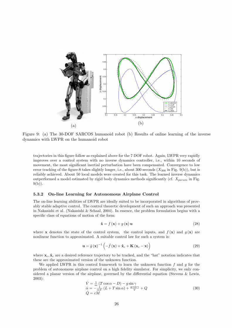
(a)
0.1 0.15 0.2 0.25 0.3 0.35 0.4 0.45 0.50
0.05
0.1
0.15
0.2
0.25
0.3
0.35
0.4
x displacement
z di
spla
cem
ent
X_desiredX_nouffX_paramX_10sX_300s
(b)
Figure 9: (a) The 30-DOF SARCOS humanoid robot (b) Results of online learning of the inversedynamics with LWPR on the humanoid robot
trajectories in this figure follow as explained above for the 7 DOF robot. Again, LWPR very rapidlyimproves over a control system with no inverse dynamics controller, i.e., within 10 seconds ofmovement, the most significant inertial perturbation have been compensated. Convergence to lowerror tracking of the figure-8 takes slightly longer, i.e., about 300 seconds (X300 in Fig. 9(b)), but isreliably achieved. About 50 local models were created for this task. The learned inverse dynamicsoutperformed a model estimated by rigid body dynamics methods significantly (cf. Xparam in Fig.9(b)).
5.3.2 On-line Learning for Autonomous Airplane Control
The on-line learning abilities of LWPR are ideally suited to be incorporated in algorithms of prov-ably stable adaptive control. The control theoretic development of such an approach was presentedin Nakanishi et al. (Nakanishi & Schaal, 2004). In essence, the problem formulation begins with aspecific class of equations of motion of the form:
x = f (x) + g (x)u (28)
where x denotes the state of the control system, the control inputs, and f (x) and g (x) arenonlinear function to approximated. A suitable control law for such a system is:
u = g (x)−1(−f (x) + xc + K (xc − x)
)(29)
where xc, xc are a desired reference trajectory to be tracked, and the “hat” notation indicates thatthese are the approximated version of the unknown function.
We applied LWPR in this control framework to learn the unknown function f and g for theproblem of autonomous airplane control on a high fidelity simulator. For simplicity, we only con-sidered a planar version of the airplane, governed by the differential equation (Stevens & Lewis,2003):
V = 1m (T cosα−D)− g sin γ
α = − 1mV (L + T sin α) + g cos γ
V + Q
Q = cM
(30)
26

In these equations, V denotes the forward speed of the airplane, m the mass, T the thrust, αthe angle of attack, g the gravity constant, γ the flight path angle w.r.t. the horizontal worldcoordinate system axis, Q the pitch rate, and c an inertial constant. The complexity of theseequations is hidden in D,L, and M , which are the unknown highly nonlinear aerodynamic dragforce, lift force, and pitch moment terms, which are specific to every airplane.
While we will not go into the detail of provably stable adaptive control with LWPR in this paperand how the control law eq.(29) is applied for airplane control, from the viewpoint of learning, themain component to learn are the lift and drag forces, and the pitch moment. These can be obtainedby re-arranging eq.(30) to:
fD (α, Q, V, M, γ, δOFL, δOFR, δMFL, δMFR, δSPL, δSPR) = T cos α−(V + g sin γ
)m
fL (α, Q, V, M, γ, δOFL, δOFR, δMFL, δMFR, δSPL, δSPR) =(g cos γ
V+ Q− α
)mV − T sin α
fM (α, Q, V, M, γ, δOFL, δOFR, δMFL, δMFR, δSPL, δSPR) =Q
c, (31)
where fD, fL and fM refer to the approximated functions of drag (forces), lift (forces) and pitch(moments).The δ terms denote the control surface angles of the airplane, with indices Midboard-Flap-Left/Right(MFL, MFR), Outboard-Flap-Left/Right (OFL, OFR), and left and right spoilers (SPL, SPR). Allterms on the right hand side of eqs.(31) are known, such that we have to cope with three simulta-neous function approximation problems in an 11-dimensional input space, an ideal application forLWPR.
We implemented LWPR for the three function above in a high fidelity simulink simulationof an autonomous airplane using the adaptive control approach of (Nakanishi & Schaal, 2004).The airplane started with now initial knowledge, just the proportional controller term in eq.(29)(i.e., the term multiplied by K). The task of the controller was to fly doublets, i.e., up-and-downtrajectories, which are essentially sinusoid-like variations of the flight path angle γ
Fig. 10 demonstrates the results of this experiment. Fig. 10(a) shows the desired trajectory inγ and its realization by the controller. Fig. 10(b,c,d) illustrate the on-line function approximationof D, L, and M . As can be seen, the control of γ achieves almost perfect tracking after just veryfew seconds. The function approximation of D and L very accurate after a very short time. Theapproximation M requires longer time for convergence, but progresses fast. About 10 local modelswere needed for learning fD and fL, while about 20 local models were allocated for fM .
An interesting element of Fig. 10 happens after 400 seconds of flight, where we simulated afailure of the airplane mechanics by locking the MFR to 17 degree deflection. As can be seen,the function approximators very quickly re-organize after this change, and the flight is successfullycontinued, although γ tracking has some error for a while until it converges back to good trackingperformance. The strong signal changes in the first seconds after the failure are due to oscillationsof the control surfaces, and not a problem in function approximation. Without adaptive control,the airplane would have crashed.
6 Discussion
Nonparametric regression with spatially localized models remains one of the most data-efficientand computationally efficient methods for incremental learning with automatic determination ofthe model complexity. In order to overcome the curse of dimensionality of local learning systems,this paper investigated methods of linear projection regression and how to employ them in spatiallylocalized nonlinear function approximation for high-dimensional input data that has redundantand irrelevant components. We compared various local dimensionality reduction techniques – ananalysis that resulted in choosing a localized version of Partial Least Squares regression at thecore of a novel nonparametric function approximator, Locally Weighted Projection Regression
27

-0.4-0.3-0.2-0.1
00.10.20.30.40.5
0 100 200 400 500 600Time [s]
L L_pred
0.01
0.02
0.03
0.04
0.05
0.06
0 100 200 400 500 600Time [s]
D D_pred
0.002
-8
-6
-4
-2
0
2
4
6
0 100 200 400 500 600Time [s]
Gamma_desired Gamma(a)
(b)
(c)
Figure 10: LWPR learning results for adaptive learning control on a simulated autonomous airplane:(a) tracking of flight angle γ, (b) approximation of lift force, (c) approximation of drag force, (d)approximation of pitch moment. At 400 seconds into the flight, a failure is simulated that locks onecontrol surface to a 17 degree angle. Note that for reasons of clearer illustration, an axis break wasinserted after 200 seconds.
28

(LWPR). The proposed technique was evaluated on a range of artificial and real world data sets inup to 50 dimensional input spaces. Besides showing fast and robust learning performance due tosecond order learning methods based on stochastic leave-one-out cross validation, LWPR exceledby its low computational complexity: updating each local model with a new data point remainedlinear in its computational cost in the number of inputs since the algorithm accomplishes goodapproximation results with only 3-4 projections irrespective of the number of input dimensions. Toour knowledge, this is the first spatially localized incremental learning system that can efficientlywork in high dimensional spaces and that is thus suited for on-line and real-time applications. Inaddition, LWPR compared favorably in its generalization performance with state-of-the-art batchregression regression methods like Gaussian Process Regression, and can provide qualitiativelysimilar estimates of confidence bounds and predictive variances.
The major drawback of LWPR in its current form is the need for gradient descent to optimize thelocal distance metrics in each local model, and the manual tuning of a forgetting factor as requiredin almost all recurisve learning algorithms that accumulate sufficient statistics. Future work willderive a probabilistic version of partial least squares regression that will allow a complete Bayesiantreatment of nonparametric regression with locally linear models, hopefully with no remaining openparameters for manual adjustment. Whether a full Bayesian version of LWPR can achieve the samecomputational efficiency as the nonparametric implemention, however, remains to be seen.
Appendix
A Pseudocode for PLS/PCR/CPR regression
PLS/PCR/CPR Pseudocode (a)
1. Initialize: Xres = X, yres = y
2. for i = 1 to k do
(a) Xt = XresT, where T is a diagonal weight matrix.(b) If [PLS]: ui = XT
t yres.If [PCR/CPR]: ui = [eig vec(XT
t Xt)]max.(c) βi = sT
i yres/(sTi si) where si = Xresui.
(d) yres = yres − siβi.(e) Xres = Xres − sipi
T where pi = XTressi/(sT
i si).
where T = I for PLS and PCR.
Locally Weighted version of PLS/PCR/CPR regression (b)
1. Initialize: Xres = X, yres = y
2. for i = 1 to k do
(a) Xt = XresT, where T is a diagonal weight matrix.(b) If [PLS]: ui = WXT
t yres.If [PCR/CPR]: ui = [eig vec(XT
t WXt)]max.(c) βi = WsT
i yres/(sTi Wsi) where si = Xresui.
(d) yres = yres − siβi.(e) Xres = Xres − sipi
T where pi = WXTressi/(sT
i Wsi).
29

B PRESS residuals for PLS
We prove that, under the assumption that x lives in a reduced dimensional subspace, the PRESSresiduals of Eq.(21) can indeed be replaced by the residual denoted by Eq.(22), i.e.
xTi Pxi = zT
i Pzzi (32)
where P = (XT X)−1, Pz = (ZT Z)−1 corresponds to the inverse covariance matrices.(Refer to Table 1 for the batch notations.)Part 1: Let T be the transformation matrix with full rank in row space that denotes coordinatetransformation from the rank deficient space of x to the full rank space of z. Then, for any z = TT xand the corresponding inverse covariance matrix Pz, we can show that
zTi Pzzi = xT
i T((XT)T (XT))−1TT xi = xTi (XT X)−1xi = xT
i Pxi (33)
i.e., a linear transformation maintains the norm.Part 2: In this part, we will show that the recursive PLS projections which transform the inputs xto z can be written as a linear transformation matrix, which completes our proof. Clarifying someof the notation:
X ≡ [x1 x2 . . . xM ]T , Z ≡ [z1 z2 . . . zM ]T ≡ [s1 s2 . . . sk]. (34)
We will now look at each of the k PLS projection directions and attempt to show that zi = TT xi
or (in a batch sense) Z = XT by showing (for each individual projections) k, there exists a tk suchthat:
sk = Xtk, where T = [t1 t2 . . . tk]. (35)
For k = 1 (c.f. Table 3),s1 = XXT y = Xt1, where t1 = XT y. (36)
For k = 2 (c.f. Table 3),s2 = XresXT
resyres (37)
We also know from the algorithm (c.f. Table 3) that,
Xres = X− s1sT1 X
sT1 s1
= (I− s1sT1
sT1 s1
)X = Ps1X (38)
yres = y − s1sT1 y
sT1 s1
= (I− s1sT1
sT1 s1
)y = Ps1y (39)
where Ps1 represents a projection operator. Using results from Eq.(38) and Eq.(39) in Eq.(37),
s2 = Ps1X(Ps1X)T Ps1y
= Ps1XXT Ps1y . . . using property of projection operator: Ps1 = PTs1 = Ps1Ps1
= Ps1Xt′2 (40)
It can be shown easily by writing out the psuedo inversion that there exists an operator R2 =(I− u1ut
1XT X/uT
1 XT Xu1) such that
Ps1X = XR2 (41)
Using Eqs.(40) and (41), we can write
s2 = Xt2 where t2 = R2t′2 = (I − u1ut1X
T XuT
1 XT Xu1)XT Ps1y. (42)
30

This operation can be carried out recursively to determine all the tk, showing that the PLS pro-jections can be written as a linear transformation. This completes the proof of the validity of themodified PRESS residual of Eq.(32) for PLS projections.
Also note that, Pz is diagonal by virtue of the fact that in the PLS algorithm, after everyprojection iteration, the projected components of input space X is subtracted before computingthe next projection (Table 1(c) or Table 3(2b.3)), ensuring the next component of Z will always beorthogonal to the previous ones. This property was discussed in (Frank, 1993).
C Distance Metric Update for PLS 1
M∑
i=1
∂J1
∂w=
e2cv
Wn+1− 2
z(1) e
Wn+1an+1zz,1
anH − 2
z(1)2
Wn+1(an+1zz,1)2
anR −
an+1E
(Wn+1)2
+[an+1T − 2
an+1R an+1
C
an+1zz,1
](I− u1uT
1 /(uT1 u1))x res1
Wn+1√
uT1 u1
an+1C = λan
C + wz(1)xT ; an+1H = λHn +
w ecvz(1)
(1− h)
an+1R = λan
R +w2z(1)2e2
cv
(1− h)where h =
w z(1)2
an+1zz,1
an+1E = λan
E + we2cv; an+1
T = λanT +
w(2 w e2cvz(1)/an+1
zz,1 − ecvβn+11 )
(1− h)xT
D Combined predictive variances
The noise model for combining prediction from individual local model is:
yq,k = yq + ε1 + ε2,k
where ε1 ∼ N(0, σ2/wk) and ε2,k ∼ N(0, σ2pred,k/wk). The mean prediction due to multiple local
models can be written according to a heterscedastic average:
yq =∑
k
(wk
σ2 + σ2pred,k
yq,k)/∑
k
(wk
σ2 + σ2pred,k
) ≈∑
k wkyq,k∑k wk
≈∑
k wkyq,k∑k wk
(43)
under the assumption that (σ2+σ2pred,k) is approximately constant for all contributing models k and
that yq,k is an estimate over multiple noisy instances of yq,k that has averaged out the noise processε2,k – exactly what happens within each local model. Thus, eq.(43) is consistent with eq.(19) underthe proposed dual noise model. The combined predictive variance can now be derived as:
σ2pred = Ey2
q − (Eyq)2 = E(∑
k wkyq,k∑k wk
)2 − (Eyq)2
=1
(∑
k wk)2E(
∑
k
wkyq)2 + (∑
k
wkε1)2 + (∑
k
wkε2,k)2 − (yq)2
=1
(∑
k wk)2E(
∑
k
wkε1)2 + (∑
k
wkε2,k)2 (44)
31

Using the fact that Ex2 = (Ex)2 + var(x) and noting that ε1 and ε2,k have zero mean,
σ2pred =
1(∑
k wk)2var(
∑
k
wkε1) +1
(∑
k wk)2var(
∑
k
wkε2,k)
=1
(∑
k wk)2[∑
k
w2k
σ2
wk] +
1(∑
k wk)2[∑
k
w2k
σ2pred,k
wk]
σ2pred =
∑k wkσ2
(∑
k wk)2+
∑k wkσ2
pred,k
(∑
k wk)2(45)
which gives the expression for the combined predictive variances.
E References
An, C. H., A. C., & Hollerbach, J. (1988). Model based control of a robot manipulator. MIT Press.Atkeson, C., Moore, A., & Schaal, S. (1997). Locally weighted learning. Artificial Intelligence
Review, 11 (4), 76–113.Bell, A., & Sejnowski, T. (1997). The Independent Components of natural scenes are edge filters.
Vision Research, 37 (23), 3327–3338.Belsley, D. A., K. E., & Welsch, D. (1980). Regression diagnostics. John Wiley.D’Souza, A., V. S., & Schaal, S. (2001). Are internal models of the entire body learnable? Society
for Neuroscience Abstracts, Vol. 27.Everitt, B. S. (1984). An introduction to latent variable models. Chapman and Hall, London.Fahlman, S. E., & Lebiere, C. (1990). The cascade-correlation learning architecture. In D. S.
Touretzky (Ed.), Advances in Neural Information Processing Systems 2 (pp. 524–532). Morgan-Kaufmann, Los Altos CA.
Frank, I. E., a. (1993). A statistical view of some chemometric regression tools. Technometrics,35 (2), 109–135.
Friedman, J. H., & Stutzle, W. (1981). Projection pursuit regression. Journal of America. StatisticalAssociation, 76 , 817–823.
Gelman, A. B., C. J. S. S. H. S., & Rubin, D. B. (1995). Bayesian data analysis. Chapman andHall.
Ghahramani, Z., & Beal, M. (2000). Variational inference for bayesian mixtures of factor analysers.In K. M. T.K. Leen,S. A. Solla (Ed.), Advances in Neural Information Processing Systems 12(pp. 449–455). MIT Press.
Gibbs, M., & Mackay, D. J. C. (1997). Efficient implementation of gaussian processes (Technicalreport). Cavendish Laboratory, Cambridge, UK.
Hastie, T., & Loader, C. (1993). Local regression: Automatic kernel carpentry. Statistical Science,8 , 120–143.
Hastie, T., & Tibshirani, R. (1990). Generalized additive models. Chapman and Hall, London.Hettich, S., & Bay, S. (1999). The uci kdd archive. Univeristy of California, Irvine, Department of
Information and Computer Science.Horn, R., & Johnson, C. (1994). Matrix analysis. Press Syndicate of the University of Cambridge.Jordan, M., & Jacobs, R. (1994). Hierarchical mixture of experts and the EM algorithm. Neural
Computation, 6 (2), 181–214.Kawato, M. (1999). Internal models fot motor control and trajectory planning. Current Opinions
in Neurobiology, 9 , 718–727.Ljung, L., & Soderstrom, T. (1986). Theory and prcatice of recursive identification. MIT Press.
32

Massy, W. F. (1965). Pricipal component regression in exploratory statistical research. Jornal ofthe American statistical Association, 60 , 234–246.
Myers, R. H. (1990). Classical and modern regression with applications. PWS - Kent.Nakanishi, J., F. J. A., & Schaal, S. (2004). Composite adaptive control with locally weighted
statistical learning. IEEE International Conference on Robotics and Automation (pp. 2647–2652).
Olshausen, B. A., & Field, D. J. (1996). Emergence of simple-cell receptive eld properties bylearning a sparse code for natural images. Nature, 381 , 607–609.
Perrone, M. P., & Cooper, L. N. (1993). Neural networks for speech and image processing, Chap.When Networks disagree: Ensemble methods for hybrid neural networks. Chapman Hall.
Roweis, S., & Saul, L. (2000). Nonlinear dimensionality reduction by local linear embedding.Science, 290 , 2323–2326.
Rubin, D., & Thayer, D. (1982). EM algorithms for ML factor analysis. Psychometrika, 47 (1),69–76.
Sanger, T. (1989). Optimal unsupervised learning in a single layer feedforward neural network.Neural Networks, 2 , 459–473.
Saunders, C., S. M. W. J. B. L. B., & Smola, A. (1998). Support vector machine - reference manual(Technical Report TR CSD-TR-98-03). Dept. of Computer Science, Royal Holloway, Univ. ofLondon.
Schaal, S., & Atkeson, C. (1994). Assessing the quality of learned local models. Advances in NeuralInformation Processing Systems 6 (pp. 160–167). Morgan-Kaufmann.
Schaal, S., & Atkeson, C. (1997). Receptive field weighted regression (Technical report tr-h-209).ATR Human Information Processing, Kyoto, Japan.
Schaal, S., & Atkeson, C. (1998). Constructive incremental learning from only local information.Neural Computation, 10 (8), 2047–2084.
Schaal, S., & Sternad, D. (2001). Origins and violoations of the 2/3 power law in rhythmic 3dmovements. Experimental Brain Research, 136 , 60–72.
Scholkopf, B., B. C., & Smola, A. J. (1999). Advances in kernel methods: Support vector learning.MIT Press.
Scholkopf, B., S. A. J. W. R., & Bartlett, P. (2000). New support vector algorithms. NeuralComputation, 12 (5), 1207–1245.
Scott, D. (1992). Multivariate density estimation. Wiley-NY.Smola, A. J., & Scholkopf, B. (1998). A tutorial on support vector regression (NEUROCOLT
Technical Report NC-TR-98-030). Royal Holloway College, London.Stevens, B. L., & Lewis, F. L. (2003). Aircraft control and simulation. John Wiley, New Jersey.Tenenbaum, J., d. S. V., & Langford, J. (2000). A global geometric framework for nonlinear
dimensionality reduction. Science, 290 , 2319–2323.Tipping, M., & Bishop, C. (1999). Probabilistic principal component analysis. Journal of the Royal
Statistical Society Series B, 61 (3), 611–622.Ueda, N., N. R. G. Z., & Hinton, G. (2000). SMEM algorithm for mixture models. Neural
Computation, 12 , 2109–2128.Vijayakumar, S., & Ogawa, H. (1999). RKHS based functional analysis for exact incremental
learning. Neurocomputing, 29 (1–3), 85–113.Vijayakumar, S., & Schaal, S. (1998). Local Adaptive Subspace Regression. Neural Processing
Letters, 7 (3), 139–149.Vijayakumar, S., & Schaal, S. (2000). O(n) algorithm for incremental real time learning in high
dimensional space. International Conference on Machine Learning (ICML) (pp. 1079–1086).Vlassis, N., M. Y. K. B. (2002). Supervised dimensionality reduction of intrinsically low-dimensional
data. Neural Computation.
33

Williams, C. K. I., & Rasmussen, C. (1996). Gaussian processes for regression. In M. Touretzky,& Hasselmo (Eds.), Advances in Neural Information Processing Systems 8. MIT Press.
Williams, C. K. I., & Seeger, M. (2001). Using the Nystrom method to speedup kernel machines.Advances in Neural Information Processing Systems 13. MIT Press.
Wold, H. (1975). Perspectives in probability and statistics, Chap. Soft modelling by latent variables:the nonlinear iterative partial least squares approach. Chapman Hall.
Xu, L., Jordan, M., & Hinton, G. (1995). An alternative model for mixtures of experts. In G.Tesauro, D. Touretzky, & T. Leen (Eds.), Advances in Neural Information Processing Systems,Vol. 7 (pp. 633–640). The MIT Press.
34