incremental proximal methods for larg e scale conv ex

Incremental proximal methods forlarge scale convex optimization

The MIT Faculty has made this article openly available. Please share how this access benefits you. Your story matters.

Citation Bertsekas, Dimitri P. “Incremental proximal methods for large scaleconvex optimization.” Mathematical Programming 129.2 (2011):163-195.

As Published http://dx.doi.org/10.1007/s10107-011-0472-0

Publisher Springer-Verlag

Version Author's final manuscript

Citable link http://hdl.handle.net/1721.1/73452

Terms of Use Creative Commons Attribution-Noncommercial-Share Alike 3.0

Detailed Terms http://creativecommons.org/licenses/by-nc-sa/3.0/

https://libraries.mit.edu/forms/dspace-oa-articles.html

http://hdl.handle.net/1721.1/73452

http://creativecommons.org/licenses/by-nc-sa/3.0/

Noname manuscript No.(will be inserted by the editor)

Incremental Proximal Methods for Large Scale ConvexOptimization

Dimitri P. Bertsekas

the date of receipt and acceptance should be inserted later

Abstract We consider the minimization of a sumPmi=1 fi(x) consisting of a large

number of convex component functions fi. For this problem, incremental meth-ods consisting of gradient or subgradient iterations applied to single componentshave proved very effective. We propose new incremental methods, consisting ofproximal iterations applied to single components, as well as combinations of gra-dient, subgradient, and proximal iterations. We provide a convergence and rateof convergence analysis of a variety of such methods, including some that involverandomization in the selection of components. We also discuss applications in afew contexts, including signal processing and inference/machine learning.

Keywords proximal algorithm, incremental method, gradient method, convex

Mathematics Subject Classification (2010) 90C33,90C90

1 Introduction

In this paper we focus on problems of minimization of a cost consisting of a largenumber of component functions, such as

minimizemXi=1

fi(x)

subject to x ∈ X, (1)

where fi : <n 7→ <, i = 1, . . . ,m, are convex, and X is a closed convex set.1

When m, the number of component functions, is very large there is an incentive to

Lab. for Information and Decision Systems Report LIDS-P-2847, August 2010 (revised March2011); to appear in Math. Programming Journal, 2011. Research supported by AFOSR GrantFA9550-10-1-0412. Many thanks are due to Huizhen (Janey) Yu for extensive helpful discus-sions and suggestions.

The author is with the Dept. of Electr. Engineering and Comp. Science, and the Laboratoryfor Information and Decision Systems, M.I.T., Cambridge, Mass., 02139.

1 Throughout the paper, we will operate within the n-dimensional space <n with the stan-dard Euclidean norm, denoted ‖ · ‖. All vectors are considered column vectors and a prime

2 Bertsekas

use incremental methods that operate on a single component fi at each iteration,rather than on the entire cost function. If each incremental iteration tends to makereasonable progress in some “average” sense, then depending on the value of m,an incremental method may significantly outperform (by orders of magnitude) itsnonincremental counterpart, as experience has shown.

Additive cost problems of the form (1) arise in many contexts such as dualoptimization of separable problems, machine learning (regularized least squares,maximum likelihood estimation, the EM algorithm, neural network training), andothers (e.g., distributed estimation, the Fermat-Weber problem in location theory,etc). They also arise in the minimization of an expected value that depends onx and some random vector; then the sum

Pmi=1 fi(x) is either an expected value

with respect to a discrete distribution, as for example in stochastic programming,or is a finite sample approximation to an expected value. The author’s paper [16]surveys applications that are well-suited for the incremental approach. In the casewhere the components fi are differentiable, incremental gradient methods take theform

xk+1 = PX`xk − αk∇fik(xk)

´, (2)

where αk is a positive stepsize, PX(·) denotes projection on X, and ik is the in-dex of the cost component that is iterated on. Such methods have a long history,particularly for the unconstrained case (X = <n), starting with the Widrow-Hoffleast mean squares (LMS) method [58] for positive semidefinite quadratic compo-nent functions (see e.g., [35], [7], Section 3.2.5). For nonquadratic cost components,such methods have been used extensively for the training of neural networks underthe generic name “backpropagation methods.” There are several variants of thesemethods, which differ in the stepsize selection scheme, and the order in whichcomponents are taken up for iteration (it could be deterministic or randomized).They are related to gradient methods with errors in the calculation of the gra-dient, and are supported by convergence analyses under various conditions; seeLuo [35], Grippo [26], [27], Luo and Tseng [34], Mangasarian and Solodov [36],Bertsekas [12], [13], Solodov [54], Tseng [55]. An alternative method that alsocomputes the gradient incrementally, one component per iteration, is proposed byBlatt, Hero, and Gauchman [1]. Stochastic versions of these methods also have along history, and are strongly connected with stochastic approximation methods.The main difference between stochastic and deterministic formulations is that theformer involve sampling a sequence of cost components from an infinite populationunder some statistical assumptions, while in the latter the set of cost componentsis predetermined and finite.

Incremental gradient methods typically have a slow asymptotic convergencerate not only because they are first order gradient-like methods, but also becausethey require a diminishing stepsize [such as αk = O(1/k)] for convergence. If αkis instead taken to be constant, an oscillation whose size depends on ak typicallyarises, as shown by [35]. These characteristics are unavoidable in incremental meth-ods, and are typical of all the methods to be discussed in this paper. However,because of their frequently fast initial convergence rate, incremental methods are

denotes transposition, so x′x = ‖x‖2. Throughout the paper we will be using standard termi-nology of convex optimization, as given for example in textbooks such as Rockafellar’s [50], orthe author’s recent book [15].

Incremental Proximal Methods for Large Scale Convex Optimization 3

often favored for large problems where great solution accuracy is not of paramountimportance (see [14] and [16] for heuristic arguments supporting this assertion).

Incremental subgradient methods apply to the case where the component func-tions fi are convex and nondifferentiable. They are similar to their gradient coun-terparts (2) except that an arbitrary subgradient ∇fik(xk) of the cost componentfik is used in place of the gradient:2

xk+1 = PX`xk − αk∇fik(xk)

´. (3)

Such methods were proposed in the Soviet Union by Kibardin [30], following theearlier paper by Litvakov [33] (which considered convex nondifferentiable exten-sions of linear least squares problems) and other related subsequent proposals.These works remained unnoticed in the Western literature, where incrementalmethods were reinvented often in different contexts and with different lines ofanalysis; see Solodov and Zavriev [53], Ben-Tal, Margalit, and Nemirovski [4],Nedic and Bertsekas [39], [40], [41], Nedic, Bertsekas, and Borkar [38], Kiwiel [31],Rabbat and Nowak [48], [49], Shalev-Shwartz et. al. [52], Johansson, Rabi, andJohansson [29], Helou and De Pierro [28], Predd, Kulkarni, and Poor [44], andRam, Nedic, and Veeravalli [46], [47]. Incremental subgradient methods have con-vergence properties that are similar in many ways to their gradient counterparts,the most important similarity being the necessity of a diminishing stepsize αk forconvergence. The lines of analysis, however, tend to be different, since incrementalgradient methods rely for convergence on the decrease of the cost function value,while incremental gradient methods rely on the decrease of the iterates’ distanceto the optimal solution set. The line of analysis of the present paper is of the lattertype, similar to earlier works of the author and his collaborators (see [39], [40], [38],and the textbook presentation in [5]).

In this paper, we propose and analyze for the first time incremental methodsthat relate to proximal algorithms. The simplest one for problem (1) is of the form

xk+1 = arg minx∈X

fik(x) +

1

2αk‖x− xk‖2

ff, (4)

which bears the same relation to the proximal minimization algorithm (Martinet[37], Rockafellar [51]) as the incremental subgradient method (3) bears to theclassical subgradient method.3 Here αk is a positive scalar sequence, and weassume that each fi : <n 7→ < is a convex function and X is a closed convex set. Themotivation for this method is that with a favorable structure of the components,the proximal iteration (3) may be obtained in closed form or be relatively simple,in which case it may be preferable to a gradient or subgradient iteration. In thisconnection, we note that generally, proximal iterations are considered more stablethan gradient iterations; for example in the nonincremental case, they convergeessentially for any choice of αk, but this is not so for gradient methods.

2 In this paper, we use ∇f(x) to denote a subgradient of a convex function f at a vector x.

The choice of ∇f(x) from within ∂f(x) is clear from the context.3 In this paper we restrict attention to proximal methods with the quadratic regularization

term ‖x − xk‖2. Our approach is applicable in principle when a nonquadratic term is usedinstead in order to match the structure of the given problem. The discussion of such alternativealgorithms is beyond our scope, but the analysis of this paper may serve as a guide for theirinvestigation.

4 Bertsekas

While some cost function components may be well suited for a proximal it-eration, others may not be, so it makes sense to consider combinations of gradi-ent/subgradient and proximal iterations. In fact nonincremental combinations ofgradient and proximal methods for minimizing the sum of two functions f andh (or more generally, finding a zero of the sum of two nonlinear operators) havea long history, dating to the splitting algorithms of Lions and Mercier [32], andPassty [45], and have become popular recently (see Beck and Teboulle [9], [10], andthe references they give to specialized algorithms, such as shrinkage/thresholding,cf. Section 5.1).

In this paper we adopt a unified analytical framework that includes incre-mental gradient, subgradient, and proximal methods, and their combinations, andhighlights their common behavior. In particular, we consider the problem

minimize F (x)def=

mXi=1

Fi(x)

subject to x ∈ X, (5)

where for all i, Fi is of the form

Fi(x) = fi(x) + hi(x), (6)

fi : <n 7→ < and hi : <n 7→ < are real-valued convex (and hence continuous)functions, and X is a nonempty closed convex set. We implicitly assume here thatthe functions fi are suitable for a proximal iteration, while the functions hi arenot and thus may be preferably treated with a subgradient iteration.

One of our algorithms has the form

zk = arg minx∈X

fik(x) +

1

2αk‖x− xk‖2

ff, (7)

xk+1 = PX`zk − αk∇hik(zk)

´, (8)

where ∇hik(zk) is an arbitrary subgradient of hik at zk. Note that the iterationis well-defined because the minimum in Eq. (7) is uniquely attained since fi iscontinuous and ‖x − xk‖2 is real-valued, strictly convex, and coercive, while thesubdifferential ∂hi(zk) is nonempty since hi is real-valued. Note also that by choos-ing all the fi or all the hi to be identically zero, we obtain as special cases thesubgradient and proximal iterations (3) and (4), respectively.

Both iterations (7) and (8) maintain the sequences zk and xk within theconstraint set X, but it may be convenient to relax this constraint for eitherthe proximal or the subgradient iteration, thereby requiring a potentially simplercomputation. This leads to the algorithm

zk = arg minx∈<n

fik(x) +

1

2αk‖x− xk‖2

ff, (9)

xk+1 = PX`zk − αk∇hik(zk)

´, (10)

where the restriction x ∈ X has been omitted from the proximal iteration, and thealgorithm

zk = xk − αk∇hik(xk), (11)


xk+1 = arg minx∈X

fik(x) +

1

2αk‖x− zk‖2

ff, (12)

where the projection onto X has been omitted from the subgradient iteration. Itis also possible to use different stepsize sequences in the proximal and subgradientiterations, but for notational simplicity we will not discuss this type of algorithm.Still another possibility is to replace hik by a linear approximation in an incre-mental proximal iteration that also involves fik . This leads to the algorithm

xk+1 = arg minx∈X

fik(x) + hik(xk) + ∇hik(xk)′(x− xk) +

1

2αk‖x− xk‖2

ff, (13)

which also yields as special cases the subgradient and proximal iterations (3) and(4), when all the fi or all the hi are identically zero, respectively.

All of the incremental proximal algorithms given above are new to our knowl-edge. The closest connection to the existing proximal methods literature is the dif-ferentiable nonincremental case of the algorithm (13) (hi is differentiable, possiblynonconvex, with Lipschitz continuous gradient, and m = 1), which has been calledthe “proximal gradient” method, and has been analyzed and discussed recently inthe context of several machine learning applications by Beck and Teboulle [9], [10](it can also be interpreted in terms of splitting algorithms [32], [45]). We note thatcontrary to subgradient and incremental methods, the proximal gradient methoddoes not require a diminishing stepsize for convergence to the optimum. In fact,the line of convergence analysis of Beck and Teboulle relies on the differentiabilityof hi and the nonincremental character of the proximal gradient method, and isthus different from ours.

Aside from the introduction of a unified incremental framework within whichproximal and subgradient methods can be embedded and combined, the purposeof the paper is to establish the convergence properties of the incremental methods(7)-(8), (9)-(10), (11)-(12), and (13). This includes convergence within a certainerror bound for a constant stepsize, exact convergence to an optimal solution foran appropriately diminishing stepsize, and improved convergence rate/iterationcomplexity when randomization is used to select the cost component for iteration.In Section 2, we show that proximal iterations bear a close relation to subgradientiterations, and we use this relation to write our methods in a form that is conve-nient for the convergence analysis. In Section 3 we discuss convergence with a cyclicrule for component selection. In Section 4, we discuss a randomized componentselection rule and we demonstrate a more favorable convergence rate estimate overthe cyclic rule, as well as over the classical nonincremental subgradient method.In Section 5 we discuss some applications.

2 Incremental Subgradient-Proximal Methods

We first show some preliminary properties of the proximal iteration in the followingproposition. These properties have been commonly used in the literature, but forconvenience of exposition, we collect them here in the form we need them. Part(a) provides a key fact about incremental proximal iterations. It shows that theyare closely related to incremental subgradient iterations, with the only differencebeing that the subgradient is evaluated at the end point of the iteration rather

6 Bertsekas

than at the start point. Part (b) of the proposition provides an inequality that isuseful for our convergence analysis. In the following, we denote by ri(S) the relativeinterior of a convex set S, and by dom(f) the effective domain

˘x | f(x) < ∞

¯of

a function f : <n 7→ (−∞,∞].

Proposition 1 Let X be a nonempty closed convex set, and let f : <n 7→ (−∞,∞] be

a closed proper convex function such that ri(X) ∩ ri`dom(f)

´6= ∅. For any xk ∈ <n

and αk > 0, consider the proximal iteration

xk+1 = arg minx∈X

f(x) +

1

2αk‖x− xk‖2

ff. (14)

(a) The iteration can be written as

xk+1 = PX`xk − αk∇f(xk+1)

´, i = 1, . . . ,m, (15)

where ∇f(xk+1) is some subgradient of f at xk+1.

(b) For all y ∈ X, we have

‖xk+1 − y‖2 ≤ ‖xk − y‖2 − 2αk`f(xk+1)− f(y)

´− ‖xk − xk+1‖2

≤ ‖xk − y‖2 − 2αk`f(xk+1)− f(y)

´. (16)

Proof (a) We use the formula for the subdifferential of the sum of the three func-tions f , (1/2αk)‖x−xk‖2, and the indicator function of X (cf. Prop. 5.4.6 of [15]),together with the condition that 0 should belong to this subdifferential at theoptimum xk+1. We obtain that Eq. (14) holds if and only if

1

αk(xk − xk+1) ∈ ∂f(xk+1) +NX(xk+1), (17)

where NX(xk+1) is the normal cone of X at xk+1 [the set of vectors y such thaty′(x−xk+1) ≤ 0 for all x ∈ X, and also the subdifferential of the indicator functionof X at xk+1; see [15], p. 185]. This is true if and only if

xk − xk+1 − αk∇f(xk+1) ∈ NX(xk+1),

for some ∇f(xk+1) ∈ ∂f(xk+1), which in turn is true if and only if Eq. (15) holds,by the projection theorem.

(b) By writing ‖xk − y‖2 as ‖xk − xk+1 + xk+1 − y‖2 and expanding, we have

‖xk − y‖2 = ‖xk − xk+1‖2 − 2(xk − xk+1)′(y − xk+1) + ‖xk+1 − y‖2. (18)

Also since from Eq. (17), 1αk

(xk − xk+1) is a subgradient at xk+1 of the sum of fand the indicator function of X, we have (using also the assumption y ∈ X)

f(xk+1) +1

αk(xk − xk+1)′(y − xk+1) ≤ f(y).

Combining this relation with Eq. (18), the result follows. ut

Based on part (a) of the preceding proposition, we see that all the iterations(7)-(8), (9)-(10), and (13) can be written in an incremental subgradient format:


(a) Iteration (7)-(8) can be written as

zk = PX`xk − αk∇fik(zk)

´, xk+1 = PX

`zk − αk∇hik(zk)

´, (19)

(b) Iteration (9)-(10) can be written as

zk = xk − αk∇fik(zk), xk+1 = PX`zk − αk∇hik(zk)

´, (20)

(c) Iteration (11)-(12) can be written as

zk = xk − αk∇hik(xk), xk+1 = PX`zk − αk∇fik(xk+1)

´. (21)

Using Prop. 1(a), we see that iteration (13) can be written into the form (21),so we will not consider it further. To show this, note that by Prop. 1(b) with

f(x) = fik(x) + hik(xk) + ∇hik(xk)′(x− xk),

we may write iteration (13) in the form

xk+1 = PX`xk − αk∇fik(xk+1)− αk∇hik(xk)

´,

which is just iteration (21). Note that in all the preceding updates, the subgradient∇hik can be any vector in the subdifferential of hik , while the subgradient ∇fikmust be a specific vector in the subdifferential of fik , specified according to Prop.1(a). Note also that iteration (20) can be written as

xk+1 = PX`xk − αk∇Fik(zk)

´,

and resembles the incremental subgradient method for minimizing over X the costfunction

F (x) =mXi=1

Fi(x) =mXi=1

`fi(x) + hi(x)

´[cf. Eq. (5)], the only difference being that the subgradient of Fik is taken at zkrather than xk.

For a convergence analysis, we need to specify the order in which the compo-nents fi, hi are chosen for iteration. We consider two possibilities:

(1) A cyclic order , whereby fi, hi are taken up in the fixed deterministic order1, . . . ,m, so that ik is equal to (k modulo m) plus 1. A contiguous block of iter-ations involving f1, h1, . . . , fm, hm in this order and exactly once is calleda cycle. We assume that the stepsize αk is constant within a cycle (for all kwith ik = 1 we have αk = αk+1 = · · · = αk+m−1).

(2) A randomized order , whereby at each iteration a component pair fi, hi ischosen randomly by sampling over all component pairs with a uniform distri-bution, independently of the past history of the algorithm.4

4 Another technique for incremental methods, popular in neural network training practice,is to reshuffle randomly the order of the component functions after each cycle. This alternativeorder selection scheme leads to convergence, like the preceding two. Moreover, this scheme hasthe nice property of allocating exactly one computation slot to each component in an m-slotcycle (m incremental iterations). By comparison, choosing components by uniform samplingallocates one computation slot to each component on the average, but some components maynot get a slot while others may get more than one. A nonzero variance in the number ofslots that any fixed component gets within a cycle, may be detrimental to performance, andindicates that reshuffling randomly the order of the component functions after each cycle maywork better; this is consistent with experimental observations shared with the author by B.Recht (private communication). However, establishing this fact analytically seems difficult,and remains an open question.

8 Bertsekas

Note that it is essential to include all components in a cycle in the cyclic case,and to sample according to the uniform distribution in the randomized case, forotherwise some components will be sampled more often than others, leading to abias in the convergence process. For the remainder of the paper, we denote by F ∗

the optimal value:F ∗ = inf

x∈XF (x),

and by X∗ the set of optimal solutions (which could be empty):

X∗ =˘x∗ | x∗ ∈ X, F (x∗) = F ∗

¯.

Also, for a nonempty closed convex set X, we denote by dist(·;X) the distancefunction given by

dist(x;X) = minz∈X‖x− z‖, x ∈ <n.

In our convergence analysis of Section 4, we will use the following well-knowntheorem (see e.g., [43], [7]). We will use a simpler deterministic version of thetheorem in Section 3.

Proposition 2 (Supermartingale Convergence Theorem) Let Yk, Zk, and Wk, k =0, 1, . . ., be three sequences of random variables and let Fk, k = 0, 1, . . ., be sets of

random variables such that Fk ⊂ Fk+1 for all k. Suppose that:

(1) The random variables Yk, Zk, and Wk are nonnegative, and are functions of the

random variables in Fk.

(2) For each k, we have

E˘Yk+1 | Fk

¯≤ Yk − Zk +Wk.

(3) There holds, with probability 1,P∞k=0Wk <∞.

Then we haveP∞k=0 Zk <∞, and the sequence Yk converges to a nonnegative random

variable Y , with probability 1.

3 Convergence Analysis for Methods with Cyclic Order

In this section, we analyze convergence under the cyclic order. We consider arandomized order in the next section. We focus on the sequence xk rather thanzk, which need not lie within X in the case of iterations (20) and (21) whenX 6= <n. In summary, the idea that guides the analysis is to show that the effectof taking subgradients of fi or hi at points near xk (e.g., at zk rather than at xk)is inconsequential, and diminishes as the stepsize αk becomes smaller, as long assome subgradients relevant to the algorithms are uniformly bounded in norm bysome constant. In particular, we assume the following throughout this section.

Assumption 1 (For iterations (19) and (20)) There is a constant c ∈ < such that

for all k

max˘‖∇fik(zk)‖, ‖∇hik(zk)‖

¯≤ c. (22)

Furthermore, for all k that mark the beginning of a cycle (i.e., all k > 0 with ik = 1),

we have for all j = 1, . . . ,m,

max˘fj(xk)− fj(zk+j−1), hj(xk)− hj(zk+j−1)

¯≤ c ‖xk − zk+j−1‖. (23)


Assumption 2 (For iteration (21)) There is a constant c ∈ < such that for all k

max˘‖∇fik(xk+1)‖, ‖∇hik(xk)‖

¯≤ c. (24)

Furthermore, for all k that mark the beginning of a cycle (i.e., all k > 0 with ik = 1),

we have for all j = 1, . . . ,m,

max˘fj(xk)− fj(xk+j−1), hj(xk)− hj(xk+j−1)

¯≤ c ‖xk − xk+j−1‖, (25)

fj(xk+j−1)− fj(xk+j) ≤ c ‖xk+j−1 − xk+j‖. (26)

Note that conditions (23) and (25) are satisfied if for each j and k, there is asubgradient of fj at xk and a subgradient of hj at xk, whose norms are boundedby c. Conditions that imply the preceding assumptions are that:

(a) For algorithm (19): fi and hi are Lipschitz continuous over X.(b) For algorithms (20) and (21): fi and hi are Lipschitz continuous over <n.(c) For all algorithms (19), (20), and (21): fi and hi are polyhedral [this is a special

case of (a) and (b)].(d) The sequences xk and zk are bounded [since then fi and hi, being real-

valued and convex, are Lipschitz continuous over any bounded set that containsxk and zk (see e.g., [15], Prop. 5.4.2)].

The following proposition provides a key estimate.

Proposition 3 Let xk be the sequence generated by any one of the algorithms (19)-

(21), with a cyclic order of component selection. Then for all y ∈ X and all k that

mark the beginning of a cycle (i.e., all k with ik = 1), we have

‖xk+m − y‖2 ≤ ‖xk − y‖2 − 2αk`F (xk)− F (y)

´+ α2

kβm2c2, (27)

where β = 1m + 4 in the case of (19) and (20), and β = 5

m + 4 in the case of (21).

Proof We first prove the result for algorithms (19) and (20), and then indicate themodifications necessary for algorithm (21). Using Prop. 1(b), we have for all y ∈ Xand k,

‖zk − y‖2 ≤ ‖xk − y‖2 − 2αk`fik(zk)− fik(y)

´. (28)

Also, using the nonexpansion property of the projection [i.e.,‚‚PX(u)− PX(v)

‚‚ ≤‖u− v‖ for all u, v ∈ <n], the definition of subgradient, and Eq. (22), we obtain forall y ∈ X and k,

‖xk+1 − y‖2 =‚‚PX`zk − αk∇hik(zk)

´− y‚‚2

≤ ‖zk − αk∇hik(zk)− y‖2

≤ ‖zk − y‖2 − 2αk∇hik(zk)′(zk − y) + α2k

‚‚∇hik(zk)‚‚2

≤ ‖zk − y‖2 − 2αk`hik(zk)− hik(y)

´+ α2

kc2. (29)

Combining Eqs. (28) and (29), and using the definition Fj = fj + hj , we have

‖xk+1 − y‖2 ≤ ‖xk − y‖2 − 2αk`fik(zk) + hik(zk)− fik(y)− hik(y)

´+ α2

kc2

= ‖xk − y‖2 − 2αk`Fik(zk)− Fik(y)

´+ α2

kc2. (30)

10 Bertsekas

Let now k mark the beginning of a cycle (i.e., ik = 1). Then at iterationk+j−1, j = 1, . . . ,m, the selected components are fj , hj, in view of the assumedcyclic order. We may thus replicate the preceding inequality with k replaced byk + 1, . . . , k +m− 1, and add to obtain

‖xk+m − y‖2 ≤ ‖xk − y‖2 − 2αk

mXj=1

`Fj(zk+j−1)− Fj(y)

´+mα2

kc2,

or equivalently, since F =Pmj=1 Fj ,

‖xk+m − y‖2 ≤ ‖xk − y‖2 − 2αk`F (xk)− F (y)

´+mα2

kc2

+ 2αk

mXj=1

`Fj(xk)− Fj(zk+j−1)

´. (31)

The remainder of the proof deals with appropriately bounding the last term above.From Eq. (23), we have for j = 1, . . . ,m,

Fj(xk)− Fj(zk+j−1) ≤ 2c ‖xk − zk+j−1‖. (32)

We also have

‖xk−zk+j−1‖ ≤ ‖xk−xk+1‖+ · · ·+‖xk+j−2−xk+j−1‖+‖xk+j−1−zk+j−1‖, (33)

and by the definition of the algorithms (19) and (20), the nonexpansion propertyof the projection, and Eq. (22), each of the terms in the right-hand side above isbounded by 2αkc, except for the last, which is bounded by αkc. Thus Eq. (33)yields ‖xk − zk+j−1‖ ≤ αk(2j − 1)c, which together with Eq. (32), shows that

Fj(xk)− Fj(zk+j−1) ≤ 2αkc2(2j − 1). (34)

Combining Eqs. (31) and (34), we have

‖xk+m − y‖2 ≤ ‖xk − y‖2 − 2αk`F (xk)− F (y)

´+mα2

kc2 + 4α2

kc2mXj=1

(2j − 1),

and finally

‖xk+m − y‖2 ≤ ‖xk − y‖2 − 2αk`F (xk)− F (y)

´+mα2

kc2 + 4α2

kc2m2,

which is of the form (27) with β = 1m + 4.

For the algorithm (21), a similar argument goes through using Assumption2. In place of Eq. (28), using the nonexpansion property of the projection, thedefinition of subgradient, and Eq. (24), we obtain for all y ∈ X and k ≥ 0,

‖zk − y‖2 ≤ ‖xk − y‖2 − 2αk`hik(xk)− hik(y)

´+ α2

kc2, (35)

while in place of Eq. (29), using Prop. 1(b), we have

‖xk+1 − y‖2 ≤ ‖zk − y‖2 − 2αk`fik(xk+1)− fik(y)

´. (36)


Combining these equations, in analogy with Eq. (30), we obtain

‖xk+1 − y‖2 ≤ ‖xk − y‖2 − 2αk`fik(xk+1) + hik(xk)− fik(y)− hik(y)

´+ α2

kc2

= ‖xk − y‖2 − 2αk`Fik(xk)− Fik(y)

´+ α2

kc2 + 2αk

`fik(xk)− fik(xk+1)

´. (37)

As earlier, we let k mark the beginning of a cycle (i.e., ik = 1). We replicatethe preceding inequality with k replaced by k+ 1, . . . , k+m−1, and add to obtain[in analogy with Eq. (31)]

‖xk+m − y‖2 ≤ ‖xk − y‖2 − 2αk`F (xk)− F (y)

´+mα2

kc2

+ 2αk

mXj=1

`Fj(xk)− Fj(xk+j−1)

´+ 2αk

mXj=1

`fj(xk+j−1)− fj(xk+j)

´. (38)

[Note that relative to Eq. (31), the preceding equation contains an extra last term,which results from a corresponding extra term in Eq. (37) relative to Eq. (30). Thisaccounts for the difference in the value of β in the statement of the proposition.]

We now bound the two sums in Eq. (38), using Assumption 2. From Eq. (25),we have

Fj(xk)−Fj(xk+j−1) ≤ 2c‖xk−xk+j−1‖ ≤ 2c`‖xk−xk+1‖+· · ·+‖xk+j−2−xk+j−1‖

´,

and since by Eq. (24) and the definition of the algorithm, each of the norm termsin the right-hand side above is bounded by 2αkc,

Fj(xk)− Fj(xk+j−1) ≤ 4αkc2(j − 1).

Also from Eqs. (24) and (47), and the nonexpansion property of the projection,we have

fj(xk+j−1)− fj(xk+j) ≤ c ‖xk+j−1 − xk+j‖ ≤ 2αkc2.

Combining the preceding relations and adding, we obtain

2αk

mXj=1

`Fj(xk)− Fj(xk+j−1)

´+ 2αk

mXj=1

`fj(xk+j−1)− fj(xk+j)

´≤ 8α2

kc2mXj=1

(j − 1) + 4α2kc

2m

= 4α2kc

2m2 + 4α2kc

2m =

„4 +

4

m

«α2kc

2m2,

which together with Eq. (38), yields Eq. (27) with β = 4 + 5m . ut

Among other things, Prop. 3 guarantees that with a cyclic order, given theiterate xk at the start of a cycle and any point y ∈ X having lower cost than xk, thealgorithm yields a point xk+m at the end of the cycle that will be closer to y thanxk, provided the stepsize αk is sufficiently small [less than 2

`F (xk)−F (y)

´/βm2c2].

In particular, for any ε > 0 and assuming that there exists an optimal solution x∗,

either we are within αkβm2c2

2 + ε of the optimal value,

F (xk) ≤ F (x∗) +αkβm

2c2

2+ ε,

12 Bertsekas

or else the squared distance to x∗ will be strictly decreased by at least 2αkε,

‖xk+m − x∗‖2 < ‖xk − x∗‖2 − 2αkε.

Thus, using this argument, we can provide convergence results for various stepsizerules, and this is done in the next two subsections.

3.1 Convergence Within an Error Bound for a Constant Stepsize

For a constant stepsize (αk ≡ α), convergence can be established to a neighborhoodof the optimum, which shrinks to 0 as α → 0. We show this in the followingproposition.


(21), with a cyclic order of component selection, and let the stepsize αk be fixed at

some positive constant α.

(a) If F ∗ = −∞, then

lim infk→∞

F (xk) = F ∗.

(b) If F ∗ > −∞, then

lim infk→∞

F (xk) ≤ F ∗ +αβm2c2

2,

where c and β are the constants of Prop. 3.

Proof We prove (a) and (b) simultaneously. If the result does not hold, there mustexist an ε > 0 such that

lim infk→∞

F (xkm)− αβm2c2

2− 2ε > F ∗.

Let y ∈ X be such that

lim infk→∞

F (xkm)− αβm2c2

2− 2ε ≥ F (y),

and let k0 be large enough so that for all k ≥ k0, we have

F (xkm) ≥ lim infk→∞

F (xkm)− ε.

By combining the preceding two relations, we obtain for all k ≥ k0,

F (xkm)− F (y) ≥ αβm2c2

2+ ε.

Using Prop. 3 for the case where y = y together with the above relation, we obtainfor all k ≥ k0,

‖x(k+1)m− y‖2 ≤ ‖xkm− y‖2− 2α

`F (xkm)−F (y)

´+βα2m2c2 ≤ ‖xkm− y‖2− 2αε.

This relation implies that for all k ≥ k0,

‖x(k+1)m − y‖2 ≤ ‖x(k−1)m − y‖

2 − 4αε ≤ · · · ≤ ‖xk0 − y‖2 − 2(k + 1− k0)αε,

which cannot hold for k sufficiently large – a contradiction. ut

The next proposition gives an estimate of the number of iterations needed toguarantee a given level of optimality up to the threshold tolerance αβm2c2/2 givenin the preceding proposition.


Proposition 5 Let xk be a sequence generated as in Prop. 4. Then for ε > 0, we

have

min0≤k≤N

F (xk) ≤ F ∗ +αβm2c2 + ε

2, (39)

where N is given by

N = m

—dist(x0;X∗)2

αε

. (40)

Proof Assume, to arrive at a contradiction, that Eq. (39) does not hold, so thatfor all k with 0 ≤ km ≤ N , we have

F (xkm) > F ∗ +αβm2c2 + ε

2.

By using this relation in Prop. 3 with αk replaced by α and y equal to the vectorof X∗ that is at minimum distance from xkm, we obtain for all k with 0 ≤ km ≤ N ,

dist(x(k+1)m;X∗)2 ≤ dist(xkm;X∗)2 − 2α`F (xkm)− F ∗

´+α2βm2c2

≤ dist(xkm;X∗)2 − (α2βm2c2 + αε) + α2βm2c2

= dist(xkm;X∗)2 − αε.

Adding the above inequalities for k = 0, . . . , Nm , we obtain

dist(xN+m;X∗)2 ≤ dist(x0;X∗)2 −„N

m+ 1

«αε,

so that „N

m+ 1

«αε ≤ dist(x0;X∗)2,

which contradicts the definition of N . ut

According to Prop. 5, to achieve a cost function value within O(ε) of the opti-mal, the term αβm2c2 must also be of order O(ε), so α must be of order O(ε/m2c2),and from Eq. (40), the number of necessary iterations N is O(m3c2/ε2), and thenumber of necessary cycles is O

`(mc)2/ε2)

´. This is the same type of estimate as

for the nonincremental subgradient method [i.e., O(1/ε2), counting a cycle as oneiteration of the nonincremental method, and viewing mc as a Lipschitz constantfor the entire cost function F ], and does not reveal any advantage for the incre-mental methods given here. However, in the next section, we demonstrate a muchmore favorable iteration complexity estimate for the incremental methods that usea randomized order of component selection.

3.2 Exact Convergence for a Diminishing Stepsize

We also obtain an exact convergence result for the case where the stepsize αkdiminishes to zero, but satisfies

P∞k=0 αk = ∞ (so that the method can “travel”

infinitely far if necessary).

14 Bertsekas


(21), with a cyclic order of component selection, and let the stepsize αk satisfy

limk→∞

αk = 0,∞Xk=0

αk =∞.

Then,

lim infk→∞

F (xk) = F ∗.

Furthermore, if X∗ is nonempty and

∞Xk=0

α2k <∞,

then xk converges to some x∗ ∈ X∗.

Proof For the first part, it will be sufficient to show that lim infk→∞ F (xkm) = F ∗.Assume, to arrive at a contradiction, that there exists an ε > 0 such that

lim infk→∞

F (xkm)− 2ε > F ∗.

Then there exists a point y ∈ X such that

lim infk→∞

F (xkm)− 2ε > F (y).

Let k0 be large enough so that for all k ≥ k0, we have

F (xkm) ≥ lim infk→∞

F (xkm)− ε.

By combining the preceding two relations, we obtain for all k ≥ k0,

F (xkm)− F (y) > ε.

By setting y = y in Prop. 3, and by using the above relation, we have for all k ≥ k0,

‖x(k+1)m − y‖2 ≤ ‖xkm − y‖2 − 2αkmε+ βα2

kmm2c2

= ‖xkm − y‖2 − αkm“

2ε− βαkmm2c2”.

Since αk → 0, without loss of generality, we may assume that k0 is large enoughso that

2ε− βαkm2c2 ≥ ε, ∀ k ≥ k0.

Therefore for all k ≥ k0, we have

‖x(k+1)m − y‖2 ≤ ‖xkm − y‖2 − αkmε ≤ · · · ≤ ‖xk0m − y‖

2 − εkX

`=k0

α`m,

which cannot hold for k sufficiently large. Hence lim infk→∞ F (xkm) = F ∗.To prove the second part of the proposition, note that from Prop. 3, for every

x∗ ∈ X∗ and k ≥ 0 we have

‖x(k+1)m − x∗‖2 ≤ ‖xkm − x∗‖2 − 2αkm

`F (xkm)− F (x∗)

´+ α2

kmβm2c2. (41)


From the Supermartingale Convergence Theorem (Prop. 2) and the hypothesisP∞k=0 α

2k <∞, we see that

˘‖xkm−x∗‖

¯converges for every x∗ ∈ X∗.5 Since then

xkm is bounded, it has a limit point x ∈ X that satisfies

F (x) = lim infk→∞

F (xkm) = F ∗.

This implies that x ∈ X∗, so it follows that˘‖xkm − x‖

¯converges, and that the

entire sequence xkm converges to x (since x is a limit point of xkm).Finally, to show that the entire sequence xk also converges to x, note that

from Eqs. (22) and (24), and the form of the iterations (19)-(21), we have ‖xk+1−xk‖ ≤ 2αkc → 0. Since xkm converges to x, it follows that xk also convergesto x. ut

4 Convergence Analysis for Methods with Randomized Order

In this section, we analyze our algorithms for the randomized component selectionorder and a constant stepsize α. The randomized versions of iterations (19), (20),and (21), are

zk = PX`xk − α∇fωk(zk)

´, xk+1 = PX

`zk − α∇hωk(zk)

´, (42)

zk = xk − α∇fωk(zk), xk+1 = PX`zk − α∇hωk(zk)

´, (43)

zk = xk − αk∇hωk(xk), xk+1 = PX`zk − αk∇fωk(xk+1)

´, (44)

respectively, where ωk is a sequence of random variables, taking values from theindex set 1, . . . ,m.

We assume the following throughout the present section.

Assumption 3 (For iterations (42) and (43)) (a) ωk is a sequence of random

variables, each uniformly distributed over 1, . . . ,m, and such that for each k, ωkis independent of the past history xk, zk−1, xk−1, . . . , z0, x0.

(b) There is a constant c ∈ < such that for all k, we have with probability 1

max˘‖∇fi(zik)‖, ‖∇hi(zik)‖

¯≤ c, ∀ i = 1, . . . ,m, (45)

max˘fi(xk)− fi(zik), hi(xk)− hi(zik)

¯≤ c‖xk − zik‖, ∀ i = 1, . . . ,m, (46)

where zik is the result of the proximal iteration, starting at xk if ωk would be i, i.e.,

zik = arg minx∈X

fi(x) +

1

2αk‖x− xk‖2

ff,

in the case of iteration (42), and

zik = arg minx∈<n

fi(x) +

1

2αk‖x− xk‖2

ff,

in the case of iteration (43).

5 Actually we use here a deterministic version/special case of the theorem, where Yk, Zk,and Wk are nonnegative scalar sequences satisfying Yk+1 ≤ Yk − Zk + Wk with

P∞k=0 Wk <

∞. Then the sequence Yk must converge. This version is given with proof in many sources,including [7] (Lemma 3.4), and [8] (Lemma 1).

16 Bertsekas

Assumption 4 (For iteration (44)) (a) ωk is a sequence of random variables,

each uniformly distributed over 1, . . . ,m, and such that for each k, ωk is inde-

pendent of the past history xk, zk−1, xk−1, . . . , z0, x0.(b) There is a constant c ∈ < such that for all k, we have with probability 1

max˘‖∇fi(xik+1)‖, ‖∇hi(xk)‖

¯≤ c, ∀ i = 1, . . . ,m, (47)

fi(xk)− fi(xik+1) ≤ c‖xk − xik+1‖, ∀ i = 1, . . . ,m, (48)

where xik+1 is the result of the iteration, starting at xk if ωk would be i, i.e.,

xik+1 = PX`zik − αk∇fi(x

ik+1)

´,

with

zik = xk − αk∇hi(xk).

Note that condition (46) is satisfied if there exist subgradients of fi and hiat xk with norms less than or equal to c. Thus the conditions (45) and (46) aresimilar, the main difference being that the first applies to “slopes” of fi and hi atzik while the second applies to the “slopes” of fi and hi at xk. There is an analogoussimilarity between conditions (47) and (48). As in the case of Assumptions 1 and2, these conditions are guaranteed by Lipschitz continuity assumptions on fi andhi. We will first deal with the case of a constant stepsize, and then consider thecase of a diminishing stepsize.

Proposition 7 Let xk be the sequence generated by one of the randomized incre-

mental methods (42)-(44), and let the stepsize αk be fixed at some positive constant

α.

(a) If F ∗ = −∞, then with probability 1

infk≥0

F (xk) = F ∗.

(b) If F ∗ > −∞, then with probability 1

infk≥0

F (xk) ≤ F ∗ +αβmc2

2,

where β = 5.

Proof Consider first algorithms (42) and (43). By adapting the proof argument ofProp. 3 with Fik replaced by Fωk [cf. Eq. (30)], we have

‖xk+1 − y‖2 ≤ ‖xk − y‖2 − 2α`Fωk(zk)− Fωk(y)

´+ α2c2, ∀ y ∈ X, k ≥ 0.

By taking the conditional expectation with respect to Fk = xk, zk−1, . . . , z0, x0,and using the fact that ωk takes the values i = 1, . . . ,m with equal probability1/m, we obtain for all y ∈ X and k,

E˘‖xk+1 − y‖2 | Fk

¯≤ ‖xk − y‖2 − 2αE

˘Fωk(zk)− Fωk(y) | Fk

¯+ α2c2

= ‖xk − y‖2 −2α

m

mXi=1

`Fi(z

ik)− Fi(y)

´+ α2c2

= ‖xk − y‖2 −2α

m

`F (xk)− F (y)

´+

2α

m

mXi=1

`Fi(xk)− Fi(zik)

´+ α2c2. (49)


By using Eqs. (45) and (46),

mXi=1

`Fi(xk)− Fi(zik)

´≤ 2c

mXi=1

‖xk − zik‖ = 2cαmXi=1

‖∇fi(zik)‖ ≤ 2mαc2.

By combining the preceding two relations, we obtain

E˘‖xk+1 − y‖2 | Fk

¯≤ ‖xk − y‖2 −

2α

m

`F (xk)− F (y)

´+ 4α2c2 + α2c2

= ‖xk − y‖2 −2α

m

`F (xk)− F (y)

´+ βα2c2, (50)

where β = 5.The preceding equation holds also for algorithm (44). To see this note that Eq.

(37) yields for all y ∈ X

‖xk+1−y‖2 ≤ ‖xk−y‖2−2α`Fωk(xk)−Fωk(y)

´+α2c2 +2α

`fωk(xk)−fωk(xk+1)

´.

(51)and similar to Eq. (49), we obtain

E˘‖xk+1 − y‖2 | Fk

¯≤ ‖xk − y‖2 −

2α

m

`F (xk)− F (y)

´+

2α

m

mXi=1

`fi(xk)− fi(xik+1)

´+ α2c2. (52)

From Eq. (48), we have

fi(xk)− fi(xik+1) ≤ c‖xk − xik+1‖,

and from Eq. (47) and the nonexpansion property of the projection,

‖xk−xik+1‖ ≤‚‚xk−zik+α∇fi(xik+1)

‚‚ =‚‚xk−xk+α∇hi(xk)+α∇fi(xik+1)

‚‚ ≤ 2αc.

Combining the preceding inequalities, we obtain Eq. (50) with β = 5.Let us fix a positive scalar γ, consider the level set Lγ defined by

Lγ =

8<:nx ∈ X | F (x) < −γ + 1 + αβmc2

2

oif F ∗ = −∞,n

x ∈ X | F (x) < F ∗ + 2γ + αβmc2

2

oif F ∗ > −∞,

and let yγ ∈ X be such that

F (yγ) =

(−γ if F ∗ = −∞,

F ∗ + 1γ if F ∗ > −∞,

Note that yγ ∈ Lγ by construction. Define a new process xk that is identicalto xk, except that once xk enters the level set Lγ , the process terminates withxk = yγ . We will now argue that for any fixed γ, xk (and hence also xk) willeventually enter Lγ , which will prove both parts (a) and (b).

Using Eq. (50) with y = yγ , we have

E˘‖xk+1 − yγ‖2 | Fk

¯≤ ‖xk − yγ‖2 −

2α

m

`F (xk)− F (yγ)

´+ βα2c2,

18 Bertsekas

from which

E˘‖xk+1 − yγ‖2 | Fk

¯≤ ‖xk − yγ‖2 − vk, (53)

where

vk =

(2αm

`F (xk)− F (yγ)

´− βα2c2 if xk /∈ Lγ ,

0 if xk = yγ ,

The idea of the subsequent argument is to show that as long as xk /∈ Lγ , the scalarvk (which is a measure of progress) is strictly positive and bounded away from 0.

(a) Let F ∗ = −∞. Then if xk /∈ Lγ , we have

vk =2α

m

`F (xk)− F (yγ)

´− βα2c2

≥ 2α

m

„−γ + 1 +

αβmc2

2+ γ

«− βα2c2

=2α

m.

Since vk = 0 for xk ∈ Lγ , we have vk ≥ 0 for all k, and by Eq. (53) and theSupermartingale Convergence Theorem (cf. Prop. 2), we obtain

P∞k=0 vk < ∞

implying that xk ∈ Lγ for sufficiently large k, with probability 1. Therefore, in theoriginal process we have with probability 1

infk≥0

F (xk) ≤ −γ + 1 +αβmc2

2.

Letting γ →∞, we obtain infk≥0 F (xk) = −∞ with probability 1.

(b) Let F ∗ > −∞. Then if xk /∈ Lγ , we have

vk =2α

m

`F (xk)− F (yγ)

´− βα2c2

≥ 2α

m

„F ∗ +

2

γ+αβmc2

2− F ∗ − 1

γ

«− βα2c2

=2α

mγ.

Hence, vk ≥ 0 for all k, and by the Supermartingale Convergence Theorem, wehave

P∞k=0 vk < ∞ implying that xk ∈ Lγ for sufficiently large k, so that in the

original process,

infk≥0

F (xk) ≤ F ∗ +2

γ+αβmc2

2

with probability 1. Letting γ →∞, we obtain infk≥0 F (xk) ≤ F ∗ + αβmc2/2. ut


4.1 Error Bound for a Constant Stepsize

By comparing Prop. 7(b) with Prop. 4(b), we see that when F ∗ > −∞ and thestepsize α is constant, the randomized methods (42), (43), and (44), have a bettererror bound (by a factor m) than their nonrandomized counterparts. It is impor-tant to note that the bound of Prop. 4(b) is tight in the sense that for a badproblem/cyclic order we have lim infk→∞ F (xk) − F ∗ = O(αm2c2) (an examplewhere fi ≡ 0 is given in p. 514 of [5]). By contrast the randomized method will getto within O(αmc2) with probability 1 for any problem, according to Prop. 7(b).Thus the randomized order provides a worst-case performance advantage over thecyclic order: we do not run the risk of choosing by accident a bad cyclic order.Note, however, that this assessment is relevant to asymptotic convergence; thecyclic and randomized order algorithms appear to perform comparably when farfrom convergence for the same stepsize α.

A related convergence rate result is provided by the following proposition,which should be compared with Prop. 5 for the nonrandomized methods.

Proposition 8 Assume that X∗ is nonempty. Let xk be a sequence generated as in

Prop. 7. Then for any positive scalar ε, we have with probability 1

min0≤k≤N

F (xk) ≤ F ∗ +αβmc2 + ε

2, (54)

where N is a random variable with

E˘N¯≤ m dist(x0;X∗)2

αε. (55)

Proof Let y be some fixed vector in X∗. Define a new process xk which is identicalto xk except that once xk enters the level set

L =

x ∈ X

˛F (x) < F ∗ +

αβmc2 + ε

2

ff,

the process xk terminates at y. Similar to the proof of Prop. 7 [cf. Eq. (50) withy being the closest point of xk in X∗], for the process xk we obtain for all k,

E˘dist(xk+1;X∗)2 | Fk

¯≤ E

˘‖xk+1 − y‖2 | Fk

¯≤ dist(xk;X∗)2 − 2α

m

`F (xk)− F ∗

´+ βα2c2

= dist(xk;X∗)2 − vk, (56)

where Fk = xk, zk−1, . . . , z0, x0 and

vk =

(2αm

`F (xk)− F ∗

´− βα2c2 if xk 6∈ L,

0 otherwise.

In the case where xk 6∈ L, we have

vk ≥2α

m

„F ∗ +

αβmc2 + ε

2− F ∗

«− βα2c2 =

αε

m. (57)

20 Bertsekas

By the Supermartingale Convergence Theorem (cf. Prop. 2), from Eq. (56) wehave

∞Xk=0

vk <∞

with probability 1, so that vk = 0 for all k ≥ N , where N is a random variable.Hence xN ∈ L with probability 1, implying that in the original process we have

min0≤k≤N

F (xk) ≤ F ∗ +αβmc2 + ε

2

with probability 1. Furthermore, by taking the total expectation in Eq. (56), weobtain for all k,

E˘dist(xk+1;X∗)2

¯≤ E

˘dist(xk;X∗)2

¯− Evk ≤ dist(x0;X∗)2 − E

8<:kXj=0

vj

9=; ,

where in the last inequality we use the facts x0 = x0 and E˘dist(x0;X∗)2

¯=

dist(x0;X∗)2. Therefore, letting k → ∞, and using the definition of vk and Eq.(57),

dist(x0;X∗)2 ≥ E

( ∞Xk=0

vk

)= E

(N−1Xk=0

vk

)≥ E

Nαε

m

ff=αε

mE˘N¯. ut

A comparison of Props. 5 and 8 again suggests an advantage for the randomizedorder: compared to the cyclic order, it achieves a much smaller error tolerance (afactor of m), in the same expected number of iterations. Note, however, that thepreceding assessment is based on upper bound estimates, which may not be sharpon a given problem [although the bound of Prop. 4(b) is tight with a worst-caseproblem selection as mentioned earlier; see [5], p. 514]. Moreover, the comparisonbased on worst-case values versus expected values may not be strictly valid. Inparticular, while Prop. 5 provides an upper bound estimate on N , Prop. 8 providesan upper bound estimate on EN, which is not quite the same.

4.2 Exact Convergence for a Diminishing Stepsize Rule

We finally consider the case of a diminishing stepsize rule and obtain an exactconvergence result similar to Prop. 6 for the case of a randomized order selection.

Proposition 9 Let xk be the sequence generated by one of the randomized incre-

mental methods (42)-(44), and let the stepsize αk satisfy

limk→∞

αk = 0,∞Xk=0

αk =∞.

Then, with probability 1,

lim infk→∞

F (xk) = F ∗.

Furthermore, if X∗ is nonempty andP∞k=0 α

2k < ∞, then xk converges to some

x∗ ∈ X∗ with probability 1.


Proof The proof of the first part is nearly identical to the corresponding part ofProp. 6. To prove the second part, similar to the proof of Prop. 7, we obtain forall k and all x∗ ∈ X∗,

E˘‖xk+1 − x∗‖2 | Fk

¯≤ ‖xk − x∗‖2 −

2αkm

`F (xk)− F ∗

´+ βα2

kc2 (58)

[cf. Eq. (50) with α and y replaced with αk and x∗, respectively], where Fk =xk, zk−1, . . . , z0, x0. By the Supermartingale Convergence Theorem (Prop. 2),for each x∗ ∈ X∗, we have for all sample paths in a set Ωx∗ of probability 1

∞Xk=0

2αkm

`F (xk)− F ∗

´<∞, (59)

and the sequence ‖xk − x∗‖ converges.

Let vi be a countable subset of the relative interior ri(X∗) that is dense inX∗ [such a set exists since ri(X∗) is a relatively open subset of the affine hull ofX∗; an example of such a set is the intersection of X∗ with the set of vectors of theform x∗+

Ppi=1 riξi, where ξ1, . . . , ξp are basis vectors for the affine hull of X∗ and

ri are rational numbers]. The intersection Ω = ∩∞i=1Ωvi has probability 1, since itscomplement Ωc is equal to ∪∞i=1Ω

cvi

and

Prob (∪∞i=1Ωcvi) ≤

∞Xi=1

Prob (Ωcvi) = 0.

For each sample path in Ω, all the sequences˘‖xk−vi‖

¯converge so that xk is

bounded, while by the first part of the proposition [or Eq. (59)] lim infk→∞ F (xk) =F ∗. Therefore, xk has a limit point x in X∗. Since vi is dense in X∗, for everyε > 0 there exists vi(ε) such that

‚‚x− vi(ε)‚‚ < ε. Since the sequence˘‖xk − vi(ε)‖

¯converges and x is a limit point of xk, we have limk→∞

‚‚xk − vi(ε)‚‚ < ε, so that

lim supk→∞

‖xk − x‖ ≤ limk→∞

‚‚xk − vi(ε)‚‚+‚‚vi(ε) − x‚‚ < 2ε.

By taking ε→ 0, it follows that xk → x. ut

5 Applications

In this section we illustrate our methods in the context of two types of practicalapplications, and discuss relations with known algorithms.

5.1 Regularized Least Squares

Many problems in statistical inference, machine learning, and signal processinginvolve minimization of a sum of component functions fi(x) that correspond toerrors between data and the output of a model that is parameterized by a vectorx. A classical example is least squares problems, where fi is quadratic. Often a

22 Bertsekas

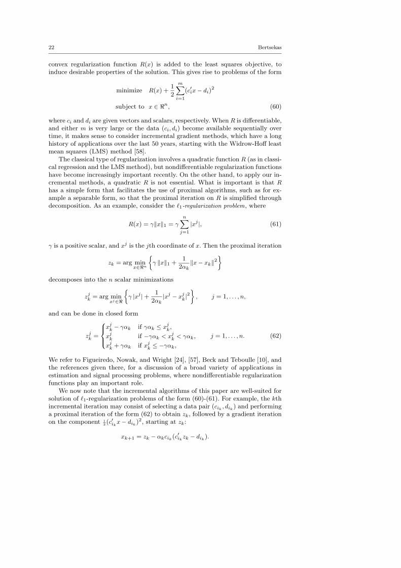
convex regularization function R(x) is added to the least squares objective, toinduce desirable properties of the solution. This gives rise to problems of the form

minimize R(x) +1

2

mXi=1

(c′ix− di)2

subject to x ∈ <n, (60)

where ci and di are given vectors and scalars, respectively. When R is differentiable,and either m is very large or the data (ci, di) become available sequentially overtime, it makes sense to consider incremental gradient methods, which have a longhistory of applications over the last 50 years, starting with the Widrow-Hoff leastmean squares (LMS) method [58].

The classical type of regularization involves a quadratic function R (as in classi-cal regression and the LMS method), but nondifferentiable regularization functionshave become increasingly important recently. On the other hand, to apply our in-cremental methods, a quadratic R is not essential. What is important is that Rhas a simple form that facilitates the use of proximal algorithms, such as for ex-ample a separable form, so that the proximal iteration on R is simplified throughdecomposition. As an example, consider the `1-regularization problem, where

R(x) = γ‖x‖1 = γnXj=1

|xj |, (61)

γ is a positive scalar, and xj is the jth coordinate of x. Then the proximal iteration

zk = arg minx∈<n

γ ‖x‖1 +

1

2αk‖x− xk‖2

ffdecomposes into the n scalar minimizations

zjk = arg minxj∈<

γ |xj |+ 1

2αk|xj − xjk|

2

ff, j = 1, . . . , n,

and can be done in closed form

zjk =

8><>:xjk − γαk if γαk ≤ x

jk,

xjk if −γαk < xjk < γαk,

xjk + γαk if xjk ≤ −γαk,

j = 1, . . . , n. (62)

We refer to Figueiredo, Nowak, and Wright [24], [57], Beck and Teboulle [10], andthe references given there, for a discussion of a broad variety of applications inestimation and signal processing problems, where nondifferentiable regularizationfunctions play an important role.

We now note that the incremental algorithms of this paper are well-suited forsolution of `1-regularization problems of the form (60)-(61). For example, the kthincremental iteration may consist of selecting a data pair (cik , dik) and performinga proximal iteration of the form (62) to obtain zk, followed by a gradient iterationon the component 1

2 (c′ikx− dik)2, starting at zk:

xk+1 = zk − αkcik(c′ikzk − dik).


This algorithm is the special case of the algorithms (19)-(21) (here X = <n,and all three algorithms coincide), with fi(x) being γ‖x‖1 (we use m copies ofthis function) and hi(x) = 1

2 (c′ix − di)2. It can be viewed as an incremental ver-

sion of a popular class of algorithms in signal processing, known as iterativeshrinkage/thresholding (see Chambolle et. al. [18], Figueiredo and Nowak [23],Daubechies, Defrise, and Mol [21], Combettes and Wajs [20], Elad, Matalon, andZibulevsky [22], Bioucas-Dias and Figueiredo [17], Vonesch and Unser [56], Beckand Teboulle [9], [10]). Our methods bear the same relation to this class of algo-rithms as the LMS method bears to gradient algorithms for the classical linearleast squares problem with quadratic regularization function.

Finally, let us note that as an alternative, the proximal iteration (62) couldbe replaced by a proximal iteration on γ |xj | for some selected index j, with allindexes selected cyclically in incremental iterations. Randomized selection of thedata pair (cik , dik) would also be interesting, particularly in contexts where thedata has a natural stochastic interpretation.

5.2 Iterated Projection Algorithms

A feasibility problem that arises in many contexts involves finding a point withcertain properties within a set intersection ∩mi=1Xi, where each Xi is a closedconvex set. For the case where m is large and each of the sets Xi has a simpleform, incremental methods that make successive projections on the component setsXi have a long history (see e.g., Gubin, Polyak, and Raik [25], and recent paperssuch as Bauschke [6], Bauschke, Combettes, and Luke [2], Bauschke, Combettes,and Kruk [3], and Cegielski and Suchocka [19], and their bibliographies). We mayconsider the following generalized version of the classical feasibility problem,

minimize f(x)

subject to x ∈ ∩mi=1Xi, (63)

where f : <n 7→ < is a convex cost function, and the method

xk+1 = PXik

`xk − αk∇f(xk)

´, (64)

where the index ik is chosen from 1, . . . ,m according to a randomized rule.The incremental approach is particularly well-suited for problems of the form (63)where the sets Xi are not known in advance, but are revealed as the algorithmprogresses. We note that incremental algorithms for problem (63), which bearsome relation with ours have been recently proposed by Nedic [42]. Actually, thealgorithm of [42] involves an additional projection on a special set X0 at eachiteration, but for simplicity we take X0 = <n.

While the problem (63) does not involve a sum of component functions, it maybe converted into one that does by using an exact penalty function. In particular,consider the problem

minimize f(x) + γ

mXi=1

dist(x;Xi)

subject to x ∈ <n, (65)

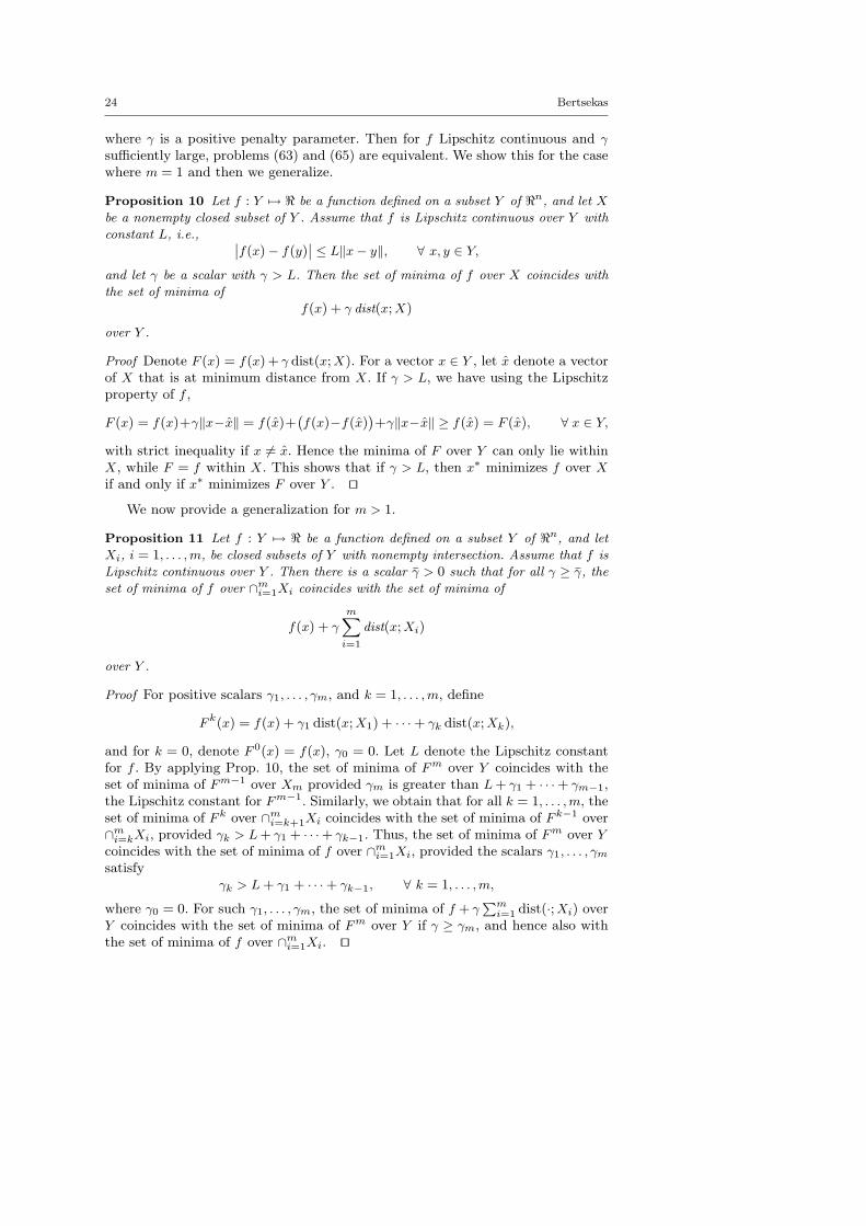
24 Bertsekas

where γ is a positive penalty parameter. Then for f Lipschitz continuous and γ

sufficiently large, problems (63) and (65) are equivalent. We show this for the casewhere m = 1 and then we generalize.

Proposition 10 Let f : Y 7→ < be a function defined on a subset Y of <n, and let X

be a nonempty closed subset of Y . Assume that f is Lipschitz continuous over Y with

constant L, i.e., ˛f(x)− f(y)

˛≤ L‖x− y‖, ∀ x, y ∈ Y,

and let γ be a scalar with γ > L. Then the set of minima of f over X coincides with

the set of minima of

f(x) + γ dist(x;X)

over Y .

Proof Denote F (x) = f(x) + γ dist(x;X). For a vector x ∈ Y , let x denote a vectorof X that is at minimum distance from X. If γ > L, we have using the Lipschitzproperty of f ,

F (x) = f(x)+γ‖x−x‖ = f(x)+`f(x)−f(x)

´+γ‖x−x‖ ≥ f(x) = F (x), ∀ x ∈ Y,

with strict inequality if x 6= x. Hence the minima of F over Y can only lie withinX, while F = f within X. This shows that if γ > L, then x∗ minimizes f over Xif and only if x∗ minimizes F over Y . ut

We now provide a generalization for m > 1.

Proposition 11 Let f : Y 7→ < be a function defined on a subset Y of <n, and let

Xi, i = 1, . . . ,m, be closed subsets of Y with nonempty intersection. Assume that f is

Lipschitz continuous over Y . Then there is a scalar γ > 0 such that for all γ ≥ γ, the

set of minima of f over ∩mi=1Xi coincides with the set of minima of

f(x) + γ

mXi=1

dist(x;Xi)

over Y .

Proof For positive scalars γ1, . . . , γm, and k = 1, . . . ,m, define

F k(x) = f(x) + γ1 dist(x;X1) + · · ·+ γk dist(x;Xk),

and for k = 0, denote F 0(x) = f(x), γ0 = 0. Let L denote the Lipschitz constantfor f . By applying Prop. 10, the set of minima of Fm over Y coincides with theset of minima of Fm−1 over Xm provided γm is greater than L+ γ1 + · · ·+ γm−1,the Lipschitz constant for Fm−1. Similarly, we obtain that for all k = 1, . . . ,m, theset of minima of F k over ∩mi=k+1Xi coincides with the set of minima of F k−1 over∩mi=kXi, provided γk > L+ γ1 + · · ·+ γk−1. Thus, the set of minima of Fm over Ycoincides with the set of minima of f over ∩mi=1Xi, provided the scalars γ1, . . . , γmsatisfy

γk > L+ γ1 + · · ·+ γk−1, ∀ k = 1, . . . ,m,

where γ0 = 0. For such γ1, . . . , γm, the set of minima of f + γPmi=1 dist(·;Xi) over

Y coincides with the set of minima of Fm over Y if γ ≥ γm, and hence also withthe set of minima of f over ∩mi=1Xi. ut


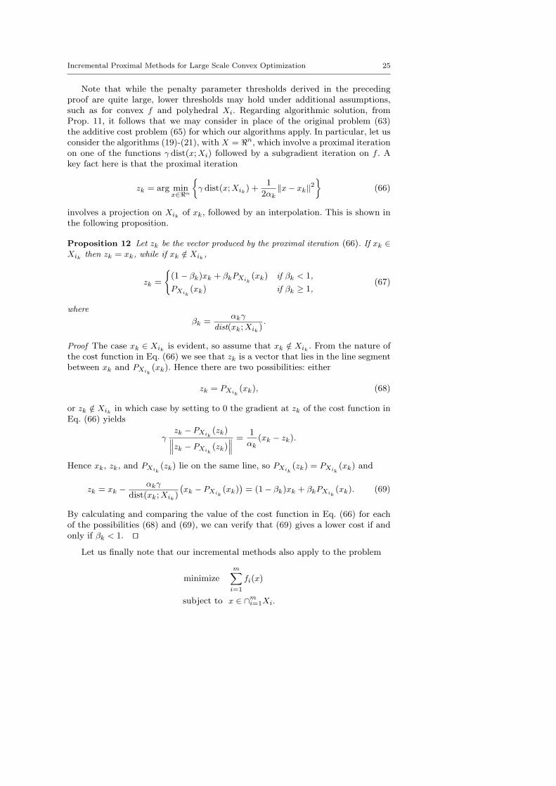
Note that while the penalty parameter thresholds derived in the precedingproof are quite large, lower thresholds may hold under additional assumptions,such as for convex f and polyhedral Xi. Regarding algorithmic solution, fromProp. 11, it follows that we may consider in place of the original problem (63)the additive cost problem (65) for which our algorithms apply. In particular, let usconsider the algorithms (19)-(21), with X = <n, which involve a proximal iterationon one of the functions γ dist(x;Xi) followed by a subgradient iteration on f . Akey fact here is that the proximal iteration

zk = arg minx∈<n

γ dist(x;Xik) +

1

2αk‖x− xk‖2

ff(66)

involves a projection on Xik of xk, followed by an interpolation. This is shown inthe following proposition.

Proposition 12 Let zk be the vector produced by the proximal iteration (66). If xk ∈Xik then zk = xk, while if xk /∈ Xik ,

zk =

((1− βk)xk + βkPXik

(xk) if βk < 1,

PXik(xk) if βk ≥ 1,

(67)

where

βk =αkγ

dist(xk;Xik).

Proof The case xk ∈ Xik is evident, so assume that xk /∈ Xik . From the nature ofthe cost function in Eq. (66) we see that zk is a vector that lies in the line segmentbetween xk and PXik

(xk). Hence there are two possibilities: either

zk = PXik(xk), (68)

or zk /∈ Xik in which case by setting to 0 the gradient at zk of the cost function inEq. (66) yields

γzk − PXik

(zk)‚‚‚zk − PXik(zk)

‚‚‚ =1

αk(xk − zk).

Hence xk, zk, and PXik(zk) lie on the same line, so PXik

(zk) = PXik(xk) and

zk = xk −αkγ

dist(xk;Xik)

`xk − PXik

(xk)´

= (1− βk)xk + βkPXik(xk). (69)

By calculating and comparing the value of the cost function in Eq. (66) for eachof the possibilities (68) and (69), we can verify that (69) gives a lower cost if andonly if βk < 1. ut

Let us finally note that our incremental methods also apply to the problem

minimizemXi=1

fi(x)

subject to x ∈ ∩mi=1Xi.

26 Bertsekas

In this case the interpolated projection iterations (67) on the sets Xi are followedby subgradient or proximal iterations on the components fi. A related problem is

minimize f(x) + c

rXj=1

max˘0, gj(x)

¯subject to x ∈ ∩mi=1Xi,

which is obtained by replacing convex inequality constraints of the form gj(x) ≤ 0with the nondifferentiable penalty terms cmax

˘0, gj(x)

¯, where c > 0 is a penalty

parameter. Then a possible incremental method at each iteration, would either doa subgradient iteration on f , or select one of the violated constraints (if any) andperform a subgradient iteration on the corresponding function gj , or select one ofthe sets Xi and do an interpolated projection on it. Except for the projections onXi, variants of this algorithm are well-known.

6 Conclusions

The incremental proximal algorithms of this paper provide new possibilities forminimization of many-term sums of convex component functions. It is generallybelieved that proximal iterations are more stable than gradient and subgradientiterations. It may thus be important to have flexibility to separate the cost func-tion into the parts that are conveniently handled by proximal iterations (e.g., inessentially closed form), and the remaining parts to be handled by subgradientiterations. We provided a convergence analysis and showed that our algorithmsare well-suited for some problems that have been the focus of recent research.

Much work remains to be done to apply and evaluate our methods within thebroad context of potential applications. Let us mention some possibilities that mayextend the range of applications of our approach, and are interesting subjects forfurther investigation: alternative proximal and projected subgradient iterations,involving nonquadratic proximal terms and/or subgradient projections, alternativestepsize rules, distributed asynchronous implementations along the lines of [38],polyhedral approximation (bundle) variants of the proximal iterations in the spiritof [11], and variants for methods with errors in the calculation of the subgradientsalong the lines of [41].

References

1. Blatt, D., Hero, A. O., Gauchman, H., 2008. “A Convergent Incremental Gradient Methodwith a Constant Step Size,” SIAM J. Optimization, Vol. 18, pp. 29-51.

2. Bauschke, H. H., Combettes, P. L., and Luke, D. R., 2003. “Hybrid Projection-ReflectionMethod for Phase Retrieval,” Journal of the Optical Soc. of America, Vol. 20, pp. 1025-1034.

3. Bauschke, H. H., Combettes, P. L., and Kruk, S. G., 2006. “Extrapolation Algorithm forAffine-Convex Feasibility Problems,” Numer. Algorithms, Vol. 41, pp. 239-274.

4. Ben-Tal, A., Margalit, T., and Nemirovski, A., 2001. “The Ordered Subsets Mirror DescentOptimization Method and its Use for the Positron Emission Tomography Reconstruction,”in Inherently Parallel Algorithms in Feasibility and Optimization and their Applications(D. Butnariu, Y. Censor, and S. Reich, eds.), Elsevier, Amsterdam, Netherlands.

5. Bertsekas, D. P., Nedic, A., and Ozdaglar, A. E., 2003. Convex Analysis and Optimization,Athena Scientific, Belmont, MA.

6. Bauschke, H. H., 2001. “Projection Algorithms: Results and Open Problems,” in InherentlyParallel Algorithms in Feasibility and Optimization and their Applications (D. Butnariu,Y. Censor, and S. Reich, eds.), Elsevier, Amsterdam, Netherlands.


7. Bertsekas, D. P., and Tsitsiklis, J. N., 1996. Neuro-Dynamic Programming, Athena Scien-tific, Belmont, MA.

8. Bertsekas, D. P., and Tsitsiklis, J. N., 2000. “Gradient Convergence in Gradient Methods,”SIAM J. Optimization, Vol. 10, pp. 627-642.

9. Beck, A., and Teboulle, M., 2009. “A Fast Iterative Shrinkage-Thresholding Algorithm forLinear Inverse Problems,” SIAM J. on Imaging Sciences, Vol. 2, pp. 183-202.

10. Beck, A., and Teboulle, M., 2010. “Gradient-Based Algorithms with Applications to Signal-Recovery Problems,” in Convex Optimization in Signal Processing and Communications (Y.Eldar and D. Palomar, eds.), Cambridge University Press, pp. 42-88.

11. Bertsekas, D. P., and Yu, H., 2009. “A Unifying Polyhedral Approximation Framework forConvex Optimization,” Lab. for Information and Decision Systems Report LIDS-P-2820,MIT; to appear in SIAM J. on Optimization.

12. Bertsekas, D. P., 1996. “Incremental Least Squares Methods and the Extended KalmanFilter,” SIAM J. on Optimization, Vol. 6, pp. 807-822.

13. Bertsekas, D. P., 1997. “A Hybrid Incremental Gradient Method for Least Squares,” SIAMJ. on Optimization, Vol. 7, pp. 913-926.

14. Bertsekas, D. P., 1999. Nonlinear Programming, 2nd edition, Athena Scientific, Belmont,MA.

15. Bertsekas, D. P., 2009. Convex Optimization Theory, Athena Scientific, Belmont, MA.16. Bertsekas, D. P., 2010. “Incremental Gradient, Subgradient, and Proximal Methods for

Convex Optimization: A Survey,” Lab. for Information and Decision Systems Report LIDS-P-2848, MIT.

17. Bioucas-Dias, J., and Figueiredo, M. A. T., 2007. “A New TwIST: Two-Step IterativeShrinkage/Thresholding Algorithms for Image Restoration,” IEEE Trans. Image Process-ing, Vol. 16, pp. 2992-3004.

18. Chambolle, A., DeVore, R. A., Lee, N. Y., and Lucier, B. J., 1998. “Nonlinear Wavelet Im-age Processing: Variational Problems, Compression, and Noise Removal Through WaveletShrinkage,” IEEE Trans. Image Processing, Vol. 7, pp. 319-335.

19. Cegielski, A., and Suchocka, A., 2008. “Relaxed Alternating Projection Methods,” SIAMJ. Optimization, Vol. 19, pp. 1093-1106.

20. Combettes, P. L., and Wajs, V. R., 2005. “Signal Recovery by Proximal Forward-BackwardSplitting,” Multiscale Modeling and Simulation, Vol. 4, pp. 1168-1200.

21. Daubechies, I., Defrise, M., and Mol, C. D., 2004. “An Iterative Thresholding Algorithmfor Linear Inverse Problems with a Sparsity Constraint,” Comm. Pure Appl. Math., Vol.57, pp. 1413-1457.

22. Elad, M., Matalon, B., and Zibulevsky, M., 2007. “Coordinate and Subspace OptimizationMethods for Linear Least Squares with Non-Quadratic Regularization,” Journal on Appliedand Computational Harmonic Analysis, Vol. 23, pp. 346-367.

23. Figueiredo, M. A. T., and Nowak, R. D., 2003. “An EM Algorithm for Wavelet-BasedImage Restoration,” IEEE Trans. Image Processing, Vol. 12, pp. 906-916.

24. Figueiredo, M. A. T., Nowak, R. D., and Wright, S. J., 2007. “Gradient Projection forSparse Reconstruction: Application to Compressed Sensing and Other Inverse Problems,”IEEE J. Sel. Topics in Signal Processing, Vol. 1, pp. 586-597.

25. Gubin, L. G., Polyak, B. T., and Raik, E. V., 1967. “The Method of Projection for Find-ing the Common Point in Convex Sets,” U.S.S.R. Comput. Math. Phys., Vol. 7, pp. 1-24(English Translation).

26. Grippo, L., 1994. “A Class of Unconstrained Minimization Methods for Neural NetworkTraining,” Optim. Methods and Software, Vol. 4, pp. 135-150.

27. Grippo, L., 2000. “Convergent On-Line Algorithms for Supervised Learning in NeuralNetworks,” IEEE Trans. Neural Networks, Vol. 11, pp. 1284-1299.

28. Helou, E. S., and De Pierro, A. R., 2009. “Incremental Subgradients for ConstrainedConvex Optimization: A Unified Framework and New Methods,” SIAM J. on Optimization,Vol. 20, pp. 1547-1572.

29. Johansson, B., Rabi, M., and Johansson, M., 2009. “A Randomized Incremental Subgradi-ent Method for Distributed Optimization in Networked Systems,” SIAM J. on Optimization,Vol. 20, pp. 1157-1170.

30. Kibardin V. M., 1980. “Decomposition into Functions in the Minimization Problem,”Automation and Remote Control, Vol. 40, pp. 1311-1323.

31. Kiwiel, K. C., 2004. “Convergence of Approximate and Incremental Subgradient Methodsfor Convex Optimization,” SIAM J. on Optimization, Vol. 14, pp. 807-840.

28 Bertsekas

32. Lions, P. L., and Mercier, B., 1979. “Splitting Algorithms for the Sum of Two NonlinearOperators,” SIAM Journal on Numerical Analysis, Vol. 16, pp. 964-979.

33. Litvakov, B. M., 1966. “On an Iteration Method in the problem of Approximating aFunction from a Finite Number of Observations,” Avtom. Telemech., No. 4, pp. 104-113.

34. Luo, Z. Q., and Tseng, P., 1994. “Analysis of an Approximate Gradient Projection Methodwith Applications to the Backpropagation Algorithm,” Optimization Methods and Soft-ware, Vol. 4, pp. 85-101.

35. Luo, Z. Q., 1991. “On the Convergence of the LMS Algorithm with Adaptive LearningRate for Linear Feedforward Networks,” Neural Computation, Vol. 3, pp. 226-245.

36. Mangasarian, O. L., and Solodov, M. V., 1994. “Serial and Parallel Backpropagation Con-vergence Via Nonmonotone Perturbed Minimization,” Opt. Methods and Software, Vol. 4,pp. 103-116.

37. Martinet, B., 1970. “Regularisation d’inequations variationelles par approximations succes-sives, Revue Fran. d’Automatique et Infomatique Rech. Operationelle, Vol. 4, pp. 154-159.

38. Nedic, A., Bertsekas, D. P., and Borkar, V., 2001. “Distributed Asynchronous IncrementalSubgradient Methods,” in Inherently Parallel Algorithms in Feasibility and Optimizationand their Applications (D. Butnariu, Y. Censor, and S. Reich, eds.), Elsevier, Amsterdam,Netherlands.

39. Nedic, A., and Bertsekas, D. P., 2000. “Convergence Rate of the Incremental SubgradientAlgorithm,” in Stochastic Optimization: Algorithms and Applications, Eds., S. Uryasev andP. M. Pardalos, Kluwer Academic Publishers.

40. Nedic, A., and Bertsekas, D. P., 2001. “Incremental Subgradient Methods for Nondiffer-entiable Optimization,” SIAM J. on Optimization, Vol. 12, 2001, pp. 109–138.

41. Nedic, A., and Bertsekas, D. P., 2010. “The Effect of Deterministic Noise in SubgradientMethods,” Math. Programming, Ser. A, Vol. 125, pp. 75-99.

42. Nedic, A., 2010. “Random Projection Algorithms for Convex Minimization Problems,”Univ. of Illinois Report; to appear in Math. Programming Journal.

43. Neveu, J., 1975. Discrete Parameter Martingales, North-Holland, Amsterdam, The Nether-lands.

44. Predd, J. B., Kulkarni, S. R., and Poor, H. V., 2009. “A Collaborative Training Algorithmfor Distributed Learning,” IEEE Transactions on Information Theory, Vol. 55, pp. 1856-1871.

45. Passty, G. B., 1979. “Ergodic Convergence to a Zero of the Sum of Monotone Operatorsin Hilbert Space,” J. Math. Anal. Appl., Vol. 72, pp. 383-390.

46. Ram, S. S., Nedic, A., and Veeravalli, V. V., 2009. “Incremental Stochastic SubgradientAlgorithms for Convex Optimization,” SIAM Journal on Optimization, Vol. 20, pp. 691-717.

47. Ram, S. S., Nedic, A., and Veeravalli, V. V., 2010. “Distributed Stochastic SubgradientProjection Algorithms for Convex Optimization,” Journal of Optimization Theory andApplications, Vol. 147, pp. 516-545.

48. Rabbat, M. G. and Nowak, R. D., 2004. “Distributed Optimization in Sensor Networks,”in Proc. Inf. Processing Sensor Networks, Berkeley, CA, pp. 20-27.

49. Rabbat, M. G. and Nowak, R. D., 2005. “Quantized Incremental Algorithms for Dis-tributed Optimization,” IEEE J. on Select Areas in Communications, Vol. 23, pp. 798-808.

50. Rockafellar, R. T., 1970. Convex Analysis, Princeton University Press, Princeton, N. J.51. Rockafellar, R. T., 1976. “Monotone Operators and the Proximal Point Algorithm,” SIAM

Journal on Control and Optimization, Vol. 14, pp. 877-898.52. Shalev-Shwartz, S., Singer, Y., Srebro, N., and Cotter, A., 2007. “Pegasos: Primal Esti-

mated Subgradient Solver for SVM,” in ICML 07, New York, N. Y., pp. 807-814.53. Solodov, M. V. and Zavriev, S. K., 1998. “Error Stability Properties of Generalized

Gradient-Type Algorithms,” J. Opt. Theory and Appl., Vol. 98, pp. 663-680.54. Solodov, M. V., 1998. “Incremental Gradient Algorithms with Stepsizes Bounded Away

from Zero,” Comput. Opt. Appl., Vol. 11, pp. 28-35.55. Tseng, P., 1998. “An Incremental Gradient(-Projection) Method with Momentum Term

and Adaptive Stepsize Rule,” SIAM J. on Optimization, Vol. 8, pp. 506-531.56. Vonesch, C., and Unser, M., 2007. “Fast Iterative Thresholding Algorithm for Wavelet-

Regularized Deconvolution,” in Proceedings of the SPIE Optics and Photonics 2007 Con-ference on Mathematical Methods: Wavelet XII, Vol. 6701, San Diego, CA, pp. 1-5.

57. Wright, S. J., Nowak, R. D., and Figueiredo, M. A. T., 2008. “Sparse Reconstructionby Separable Approximation,” in Proceedings of the IEEE International Conference onAcoustics, Speech and Signal Processing (ICASSP 2008), pp. 3373-3376.

58. Widrow, B., and Hoff, M. E., 1960. “Adaptive Switching Circuits,” Institute of RadioEngineers, Western Electronic Show and Convention, Convention Record, Part 4, pp. 96-104.

incremental proximal methods for larg e scale conv ex

Documents