COMPUTER-AIDED DESIGN OF HORIZONTAL-AXIS

WIND TURBINE BLADES

A THESIS SUBMITTED TO THE GRADUATE SCHOOL OF NATURAL AND APPLIED SCIENCES

OF MIDDLE EAST TECHNICAL UNIVERSITY

BY

SERHAT DURAN

IN PARTIAL FULFILLMENT OF THE REQUIREMENTS FOR

THE DEGREE OF MASTER OF SCIENCE IN

MECHANICAL ENGINEERING

JANUARY 2005

Approval of the Graduate School of Natural and Applied Sciences

Prof. Dr. Canan ÖZGEN Director

I certify that this thesis satisfies all the requirements as a thesis for the degree of

Master of Science.

Prof. Dr. S. Kemal İDER Head of the Department

This is to certify that we have read this thesis and that in our opinion it is fully

adequate, in scope and quality, as a thesis for degree of Master of Science.

Asst. Prof. Dr. Tahsin ÇETİNKAYA Prof. Dr. Kahraman ALBAYRAK Co-Supervisor Supervisor

Examining Committee Members

Prof. Dr. O. Cahit ERALP (METU, ME)

Prof. Dr. Kahraman ALBAYRAK (METU, ME)

Assoc. Prof. Dr. Cemil YAMALI (METU, ME)

Asst. Prof. Dr. Tahsin ÇETİNKAYA (METU, ME)

Prof. Dr. İ. Sinan AKMANDOR (METU, AEE)

iii

I hereby declare that all information in this document has been obtained and presented in accordance with academic rules and ethical conduct. I also declare that, as required by these rules and conduct, I have fully cited and referenced all material and results that are not original to this work.

Name, Last name: Serhat DURAN

Signature :

iv

ABSTRACT

COMPUTER-AIDED DESIGN OF HORIZONTAL-AXIS

WIND TURBINE BLADES

Duran, Serhat

M.S., Department of Mechanical Engineering

Supervisor: Prof. Dr. Kahraman ALBAYRAK

Co-Supervisor: Asst. Prof. Dr. Tahsin ÇETİNKAYA

January 2005, 124 Pages,

Designing horizontal-axis wind turbine (HAWT) blades to achieve satisfactory

levels of performance starts with knowledge of the aerodynamic forces acting on

the blades. In this thesis, HAWT blade design is studied from the aspect of

aerodynamic view and the basic principles of the aerodynamic behaviors of

HAWTs are investigated.

Blade-element momentum theory (BEM) known as also strip theory, which is

the current mainstay of aerodynamic design and analysis of HAWT blades, is used

for HAWT blade design in this thesis.

Firstly, blade design procedure for an optimum rotor according to BEM theory

is performed. Then designed blade shape is modified such that modified blade will

be lightly loaded regarding the highly loaded of the designed blade and power

prediction of modified blade is analyzed. When the designed blade shape is

modified, it is seen that the power extracted from the wind is reduced about 10%

v

and the length of modified blade is increased about 5% for the same required

power.

BLADESIGN which is a user-interface computer program for HAWT blade

design is written. It gives blade geometry parameters (chord-length and twist

distributions) and design conditions (design tip-speed ratio, design power

coefficient and rotor diameter) for the following inputs; power required from a

turbine, number of blades, design wind velocity and blade profile type (airfoil

type). The program can be used by anyone who may not be intimately concerned

with the concepts of blade design procedure and the results taken from the program

can be used for further studies.

Keywords: Horizontal-Axis Wind Turbine Blades, Wind energy, Aerodynamics,

Airfoil

vi

ÖZ

YATAY EKSENLİ RÜZGAR TÜRBİN PALALARININ

BİLGİSAYAR DESTEKLİ AERODİNAMİK TASARIMI

Duran, Serhat

Yüksek Lisans, Makine Mühendisliği Bölümü

Tez Yöneticisi: Prof. Dr. Kahraman ALBAYRAK

Ortak Tez Yöneticisi: Asst. Prof. Dr. Tahsin ÇETİNKAYA

Ocak 2005, 124 Sayfa,

Yatay eksenli rüzgar türbin palalarının tasarımı, öncelikle palalara etkiyen

aerodinamik kuvvetlerin bilinmesini gerektirir. Bu çalışmada, yatay eksenli rüzgar

türbin palalarının tasarımı konusu, akışkanlar dinamiği yönünden ele alınmış ve

yatay eksenli rüzgar türbinlerinin aerodinamiği ile ilgili temek teoriler

incelenmiştir.

Bu çalışmada, yatay eksenli rüzgar türbin palalarının tasarımı için, günümüz

rüzgar türbin palalarının tasarımında en sık rastlanan yöntem olan pala elemanı

teorisinden faydalanılmıştır.

İlk olarak optimum rotora ait bir palanın tasarımı için gerekli metot

oluşturulmuştur. Daha sonra tasarımı yapılan palaya etkiyen kuvvetlerin büyük

olması dikkate alınarak, palanın geometrisi; palaya etkiyen kuvvetler azaltılacak

şekilde düzeltilmiş ve geometrisi düzeltilen yeni palaların performansı

incelenmiştir. Bu incelemede, geometrisi düzeltilen palaların performansı;

vii

optimum rotor için tasarlanmış palanın performansına oranla yaklaşık %10 azaldığı

görülmüştür. Ayrıca istenilen belirli bir türbin gücü için, geometrisi düzeltilmiş

palanın boyunun, optimum rotor için tasarımı yapılan palanın boyuna oranla

yaklaşık %5 daha uzun olması gerektiği görülmüştür.

Yatay eksenli rüzgar türbin palalarının tasarımına yönelik; kullanıcı arayüzüne

sahip, BLADESIGN isminde bir bilgisayar programı yazılmıştır. Program,

kullanıcının girdiği; istenilen türbin gücü, pala sayısı, dizayn rüzgar hızı ve pala

profile ( airfoil tipi) girdilerine göre pala geometrisi parametreleri (veter uzunluğu

ve burulma açısı dağılımları) ile dizayn şartlarındaki gerekli değerleri (dizayn uç

hız oranı, dizayn güç katsayısı ve rotor çapı) vermektedir. Program, pala tasarımı

konusunda detaylı bilgiye sahip olmayan kullanıcılarına, programın verdiği

sonuçları kullanarak başka konularda çalışmada bulunabilmesine imkan

vermektedir.

Anahtar Sözcükler: Yatay Eksenli Rüzgar Türbin Palaları, Rüzgar

Enerjisi, Aerodinamik, Pala Profili

viii

To My Family

ix

ACKNOWLEDGEMENTS

The author would like to express his deepest gratitude and appreciation to his

supervisor, Prof. Dr. Kahraman Albayrak and Co-Supervisor, Asst. Prof. Dr.

Tahsin Çetinkaya for their invaluable guidance and encouragement throughout this

study. The author especially thanks his supervisor for his patience and trust during

the study.

The author also would like to thank his colleagues and ASELSAN Inc. for

their supports.

x

TABLE OF CONTENTS

PLAGIARISM . . . . . . . . . . . . . . . . . . . . . . . . . . . . . . . . . . . . . . . . . iii

ABSTRACT. . . . . . . . . . . . . . . . . . . . . . . . . . . . . . . . . . . . . . . . . . . iv

ÖZ. . . . . . . . . . . . . . . . . . . . . . . . . . . . . . . . . . . . . . . . . . . . . . . . . . . vi

DEDICATION. . . . . . . . . . . . . . . . . . . . . . . . . . . . . . . . . . . . . . . . . viii

ACKNOWLEDGEMENTS. . . . . . . . . . . . . . . . . . . . . . . . . . . . . . . ix

TABLE OF CONTENTS. . . . . . . . . . . . . . . . . . . . . . . . . . . . . . . . . x

LIST OF FIGURES. . . . . . . . . . . . . . . . . . . . . . . . . . . . . . . . . . . . . xiii

LIST OF TABLES. . . . . . . . . . . . . . . . . . . . . . . . . . . . . . . . . . . . . . xviii

NOMENCLATURE. . . . . . . . . . . . . . . . . . . . . . . . . . . . . . . . . . . . xix

CHAPTERS

1.INTRODUCTION. . . . . . . . . . . . . . . . . . . . . . . . . . . . . . . . . . . . . 1

1.1 Objective and Scope of the Thesis. . . . . . . . . . . . . . . . . . . . . . 1

1.2 Historical Development of Windmills. . . . . . . . . . . . . . . . . . . 3

1.3 Technological Developments of Modern Wind Turbines. . . . 9

2.HORIZONTAL-AXIS WIND TURBINES. . . . . . . . . . . . . . . . . . 11

2.1 Introduction. . . . . . . . . . . . . . . . . . . . . . . . . . . . . . . . . . . . . . . 11

2.2 Horizontal-Axis Wind Turbine Concepts. . . . . . . . . . . . . . . . 11

2.3 Modern Horizontal-Axis Wind Turbines. . . . . . . . . . . . . . . . . 14

2.3.1 The rotor subsystem. . . . . . . . . . . . . . . . . . . . . . . . . . . . 17

2.3.2 The power-train subsystem. . . . . . . . . . . . . . . . . . . . . . 19

2.3.3 The nacelle structure subsystem. . . . . . . . . . . . . . . . . . 19

xi

2.3.4 The tower subsystem and the foundation. . . . . . . . . . . . 19

2.3.5 The controls. . . . . . . . . . . . . . . . . . . . . . . . . . . . . . . . . . 20

2.3.6 The balance of electrical subsystem. . . . . . . . . . . . . . . . 20

2.4 Aerodynamic Controls of HAWTs. . . . . . . . . . . . . . . . . . . . . 20

2.5 Performance Parameters of HAWTs. . . . . . . . . . . . . . . . . . . . 22

2.6 Classification of HAWTs. . . . . . . . . . . . . . . . . . . . . . . . . . . . . 23

2.7 Criteria in HAWT Design. . . . . . . . . . . . . . . . . . . . . . . . . . 24

3.AERODYNAMICS OF HAWTs. . . . . . . . . . . . . . . . . . . . . . . . . . 26

3.1 Introduction. . . . . . . . . . . . . . . . . . . . . . . . . . . . . . . . . . . . . . . 26

3.2 The Actuator Disk Theory and The Betz Limit. . . . . . . . . . . . 27

3.3 The General Momentum Theory. . . . . . . . . . . . . . . . . . . . . . . 33

3.4 Blade Element Theory. . . . . . . . . . . . . . . . . . . . . . . . . . . . . . . 44

3.5 Blade Element-Momentum (BEM) Theory. . . . . . . . . . . . . . . 50

3.6 Vortex Theory. . . . . . . . . . . . . . . . . . . . . . . . . . . . . . . . . . . . . 54

4.HAWT BLADE DESIGN. . . . . . . . . . . . . . . . . . . . . . . . . . . . . . . 62

4.1 Introduction. . . . . . . . . . . . . . . . . . . . . . . . . . . . . . . . . . . . . . . 62

4.2 The Tip-Loss Factor. . . . . . . . . . . . . . . . . . . . . . . . . . . . . . . . 63

4.3 HAWT Flow States. . . . . . . . . . . . . . . . . . . . . . . . . . . . . . . . . 66

4.4 Airfoil Selection in HAWT Blade Design. . . . . . . . . . . . . . . . 69

4.5 Blade Design Procedure . . . . . . . . . . . . . . . . . . . . . . . . . . . . . . 71

4.6 Modification of Blade Geometry. . . . . . . . . . . . . . . . . . . . . . . 80

4.6.1 Modification of Chord-Length Distribution. . . . . . . . . . 80

4.6.2 Modification of Twist Distribution. . . . . . . . . . . . . . . . 81

4.7 Power Prediction of Modified Blade Shape. . . . . . . . . . . . . . . 82

4.8 Results. . . . . . . . . . . . . . . . . . . . . . . . . . . . . . . . . . . . . . . . . . . 84

xii

5. COMPUTER PROGRAM FOR BLADE DESIGN. . . . . . . . . . . 101

5.1 Introduction. . . . . . . . . . . . . . . . . . . . . . . . . . . . . . . . . . . . . . . 101

5.2 XFOILP4. . . . . . . . . . . . . . . . . . . . . . . . . . . . . . . . . . . . . . . . . 102

5.2 BLADESIGN. . . . . . . . . . . . . . . . . . . . . . . . . . . . . . . . . . . . . 105

5.3 Sample Blade Design on BLADESIGN Program . . . . . . . . . 109

5.4 Comparison of Outputs . . . . . . . . . . . . . . . . . . . . . . . . . . . . . . 116

6. CONCLUSION . . . . . . . . . . . . . . . . . . . . . . . . . . . . . . . . . . . . . . 118

REFERENCES. . . . . . . . . . . . . . . . . . . . . . . . . . . . . . . . . . . . . . . . . 122

xiii

LIST OF FIGURES

FIGURES

Figure 1.1 Early Persian windmill. . . . . . . . . . . . . . . . . . . . . . . . . . 4

Figure 1.2 The Savonius rotor. . . . . . . . . . . . . . . . . . . . . . . . . . . . . 6

Figure 1.3 Darrieus rotor. . . . . . . . . . . . . . . . . . . . . . . . . . . . . . . . . 7

Figure 2.1 Various concepts for horizontal-axis wind turbines. . . . 12

Figure 2.2 Enfield-Andreau turbine (a) General view (b) Diagram

of the flow path. . . . . . . . . . . . . . . . . . . . . . . . . . . . . . . . . . . . . . . . . 13

Figure 2.3 Schematic of two common configurations: Upwind,

rigid hub, three-bladed and downwind, teetered, two-bladed

turbine. . . . . . . . . . . . . . . . . . . . . . . . . . . . . . . . . . . . . . . . . . . . . . . 15

Figure 2.4 Major components of a horizontal-axis wind turbine. . . 16

Figure 2.5 Nomenclature and subsystems of HAWT (a) Upwind

rotor (b) Downwind rotor. . . . . . . . . . . . . . . . . . . . . . . . . . . . . . . . 17

Figure 2.6 Typical plot of rotor power coefficient vs. tip-speed

ratio for HAWT with a fixed blade pitch. . . . . . . . . . . . . . . . . . . . 22

Figure 2.7 Representative size, height and diameter of HAWTs. . . 24

Figure 3.1 Idealized flow through a wind turbine represented by a

non-rotating, actuator disk. . . . . . . . . . . . . . . . . . . . . . . . . . . . . . . 28

Figure 3.2 Velocity and pressure distribution along streamtube. . . 31

Figure 3.3 Operating parameters for a Betz turbine. . . . . . . . . . . . . 33

Figure 3.4 Streamtube model of flow behind rotating wind

turbine blade. . . . . . . . . . . . . . . . . . . . . . . . . . . . . . . . . . . . . . . . . . 34

Figure 3.5 Geometry of the streamtube model of flow through a

HAWT rotor. . . . . . . . . . . . . . . . . . . . . . . . . . . . . . . . . . . . . . . . . . 35

xiv

Figure 3.6 Theoretical maximum power coefficients as a function

of tip-speed ratio for an ideal HAWT with and without wake

rotation. . . . . . . . . . . . . . . . . . . . . . . . . . . . . . . . . . . . . . . . . . . . . . 44

Figure 3.7 Schematic of blade elements. . . . . . . . . . . . . . . . . . . . . . 45

Figure 3.8 Blade geometry for analysis of a HAWT. . . . . . . . . . . . 46

Figure 3.9 Tip and root vortices. . . . . . . . . . . . . . . . . . . . . . . . . . . . 55

Figure 3.10 Variation of bound circulation along blade length. . . . 56

Figure 3.11 Helical vortices replaced by axial and circumferential

vortex lines. . . . . . . . . . . . . . . . . . . . . . . . . . . . . . . . . . . . . . . . . . . 57

Figure 4.1 Relationship between axial induction factor, flow state

and thrust of a rotor. . . . . . . . . . . . . . . . . . . . . . . . . . . . . . . . . . . . . 67

Figure 4.2 Variation of elemental power coefficient with relative

wind angles for different values of local tip-speed ratio. . . . . . . . . 72

Figure 4.3 Variation of optimum relative wind angle with respect

to local tip-speed ratio at optimum elemental power coefficient

for B=3. . . . . . . . . . . . . . . . . . . . . . . . . . . . . . . . . . . . . . . . . . . . . . 73

Figure 4.4 Comprasion of equation 4.5.2 with the data found for

different glide ratios. . . . . . . . . . . . . . . . . . . . . . . . . . . . . . . . . . . . 74

Figure 4.5 Chord-length distribution for the designed blade. . . . . 77

Figure 4.6 Twist distribution for the designed blade. . . . . . . . . . . . 79

Figure 4.7 Variation of power coefficient with tip-speed ratio. . . . 79

Figure 4.8 Modified blade chord-length variation along the non-

dimensionalized blade radius. . . . . . . . . . . . . . . . . . . . . . . . . . . . . 81

Figure 4.9 Modified twist distribution along non-dimensionalized

blade radius. . . . . . . . . . . . . . . . . . . . . . . . . . . . . . . . . . . . . . . . . . . 82

xv

Figure 4.10 Flow chart of the iteration procedure for determining

power coefficient of modified blade. . . . . . . . . . . . . . . . . . . . . . . . 83

Figure 4.11 Effect of number of blades on peak performance of

optimum wind turbines. . . . . . . . . . . . . . . . . . . . . . . . . . . . . . . . . . 88

Figure 4.12 Effect of Drag/Lift ratio on peak performance of an

optimum three-bladed wind turbine. . . . . . . . . . . . . . . . . . . . . . . . 88

Figure 4.13 Effect of drag and tip losses on relative wind angle

for optimum design. . . . . . . . . . . . . . . . . . . . . . . . . . . . . . . . . . . . . 89

Figure 4.14 Relative wind angle for optimum performance of

three-bladed wind turbines. . . . . . . . . . . . . . . . . . . . . . . . . . . . . . . 89

Figure 4.15 Blade chord length distribution for optimum

performance of three-bladed wind turbines. . . . . . . . . . . . . . . . . 90

Figure 4.16 Twist angle distribution for modified chord-length of

the designed blade. . . . . . . . . . . . . . . . . . . . . . . . . . . . . . . . . . . . . . 90

Figure 4.17 Chord-length distribution of a modified blade for

different tip-speed ratio. . . . . . . . . . . . . . . . . . . . . . . . . . . . . . . . . . 91

Figure 4.18 Twist distribution for modified twist of the designed

blade. . . . . . . . . . . . . . . . . . . . . . . . . . . . . . . . . . . . . . . . . . . . . . . . 91

Figure 4.19 Distribution of angle of attack for modified twist of

the designed blade. . . . . . . . . . . . . . . . . . . . . . . . . . . . . . . . . . . . . . 92

Figure 4.20 Distribution of angle of attack for modified twist and

chord-length of the designed blade. . . . . . . . . . . . . . . . . . . . . . . . . 92

Figure 4.21 Comparison of power coefficients of modified blades

with the designed blade. . . . . . . . . . . . . . . . . . . . . . . . . . . . . . . . . 93

Figure 4.22 Radial thrust coefficient variation of the designed

blade . . . . . . . . . . . . . . . . . . . . . . . . . . . . . . . . . . . . . . . . . . . . . . . 93

xvi

Figure 4.23 Radial thrust coefficient for modified twist and

chord-length of the designed blade. . . . . . . . . . . . . . . . . . . . . . . . . 94

Figure 4.24 Working range of the designed blade designed at

10λ = . . . . . . . . . . . . . . . . . . . . . . . . . . . . . . . . . . . . . . . . . . . . . . . 94

Figure 4.25 Working range of modified twist and chord-length of

the designed blade designed at 10λ = . . . . . . . . . . . . . . . . . . . . . . 95

Figure 4.26 Effect of Reynolds number on peak performance of

an optimum three-bladed turbine. . . . . . . . . . . . . . . . . . . . . . . . . . 95

Figure 4.27 Views of blade elements from root towards tip for

the designed blade. . . . . . . . . . . . . . . . . . . . . . . . . . . . . . . . . . . . . . 96

Figure 4.28 Views of blade elements from root towards tip for

the designed blade. . . . . . . . . . . . . . . . . . . . . . . . . . . . . . . . . . . . . . 96

Figure 4.29 Isometric view of the blade elements for the designed

blade. . . . . . . . . . . . . . . . . . . . . . . . . . . . . . . . . . . . . . . . . . . . . . . . 97

Figure 4.30 Isometric view of the blade elements for the designed

blade. . . . . . . . . . . . . . . . . . . . . . . . . . . . . . . . . . . . . . . . . . . . . . . . 97

Figure 4.31 Three-dimensional solid model of the designed

blade. . . . . . . . . . . . . . . . . . . . . . . . . . . . . . . . . . . . . . . . . . . . . . . . 98

Figure 4.32 Three-dimensional solid model of the designed

blade. . . . . . . . . . . . . . . . . . . . . . . . . . . . . . . . . . . . . . . . . . . . . . . . 99

Figure 5.1 Comparison of XFOIL lift coefficient data with data

in reference [5] . . . . . . . . . . . . . . . . . . . . . . . . . . . . . . . . . . . . . . . . 104

Figure 5.2 Comparison of XFOIL drag coefficient data with data

in reference [5] . . . . . . . . . . . . . . . . . . . . . . . . . . . . . . . . . . . . . . . . 104

Figure 5.3 General view of BLADESIGN. . . . . . . . . . . . . . . . . . . 108

Figure 5.4 Flow Schematic of HAWT Blade Design program. . . . 109

xvii

Figure 5.5 Comparison of power coefficient of designed and

modified blade . . . . . . . . . . . . . . . . . . . . . . . . . . . . . . . . . . . . . . . . 112

Figure 5.6 Comparison of setting angle variation of designed and

modified blade . . . . . . . . . . . . . . . . . . . . . . . . . . . . . . . . . . . . . . . . 113

Figure 5.7 Comparison of chord-length distribution of designed

and modified blade . . . . . . . . . . . . . . . . . . . . . . . . . . . . . . . . . . . . . 113

Figure 5.8 Three-dimensional view of the designed blade. . . . . . . 114

Figure 5.9 Three-dimensional view of the modified blade. . . . . . . 114

Figure 5.10 Output from the program performed for the sample

blade design case . . . . . . . . . . . . . . . . . . . . . . . . . . . . . . . . . . . . . . 115

xviii

LIST OF TABLES

TABLES

Table 1.1 Technical wind energy potential and installed capacities

in some European countries . . . . . . . . . . . . . . . . . . . . . . . . . . . . . . 9

Table 2.1 Scale classification of wind turbines. . . . . . . . . . . . . . . . 23

Table 3.1 Power coefficient, ,maxpC as a function of tip-speed ratio

λ and 2a . . . . . . . . . . . . . . . . . . . . . . . . . . . . . . . . . . . . . . . . . . . . . 43

Table 4.1Blade chord and twist distribution for an optimum

three-bladed HAWT. . . . . . . . . . . . . . . . . . . . . . . . . . . . . . . . . . . . 78

Table 4.2 Power production of a fixed rotational three-bladed

HAWT . . . . . . . . . . . . . . . . . . . . . . . . . . . . . . . . . . . . . . . . . . . . . . 100

Table 5.1 Design conditions output for designed and modified

blade . . . . . . . . . . . . . . . . . . . . . . . . . . . . . . . . . . . . . . . . . . . . . . . . 110

Table 5.2 Blade geometry output for designed and modified

blade . . . . . . . . . . . . . . . . . . . . . . . . . . . . . . . . . . . . . . . . . . . . . . . . 111

Table 5.3 Comparison of outputs for the airfoils. . . . . . . . . . . . . . 116

Table 5.4 Comparison of rotor diameters for different turbine

power outputs. . . . . . . . . . . . . . . . . . . . . . . . . . . . . . . . . . . . . . . . . 117

xix

NOMENCLATURE

PC : power coefficient of wind turbine rotor

,maxPC : maximum rotor power coefficient

TC : thrust coefficient of wind turbine rotor

rTC : local thrust coefficient for each annular rotor section

P : power output from wind turbine rotor

mi

: air mass flow rate through rotor plane

U∞ : free stream velocity of wind

relU : relative wind velocity

RU : uniform wind velocity at rotor plane

wU : uniform wind velocity at far wake

u : axial wind velocity at rotor plane

v : radial wind velocity at rotor plane

w : angular wind velocity at rotor plane

w′ : induced angular velocity due to bound vorticity of rotor blades

wu : axial wind velocity at far wake

wv : radial wind velocity at far wake

ww : angular wind velocity at far wake

A : area of wind turbine rotor

R : radius of wind turbine rotor

r : radial coordinate at rotor plane

wr : radial coordinate at far wake

hr : rotor radius at hub of the blade

ir : blade radius for the ith blade element

0p : pressure of undisturbed air

xx

up : upwind pressure of rotor

dp : downwind pressure of rotor

p′ : pressure drop across rotor plane

wp : pressure at far wake

0H : Bernoulli’s constant between free-stream and inflow

1H : Bernoulli’s constant between outflow and far wake

T : rotor thrust

Q : rotor torque

DF : drag force on an annular blade element

LF : lift force on an annular blade element

L : force on an annular element tangential to the circle swept by the rotor

DC : drag coefficient of an airfoil

LC : lift coefficient of an airfoil

,L designC : design lift coefficient of an airfoil

F : tip-loss factor

iF : tip-loss factor for the ith blade element

N : number of blade elements

B : number of blades of a rotor

a : axial induction factor at rotor plane

b : axial induction factor at far wake

a′ : angular induction factor

λ : tip-speed ratio of rotor

dλ : design tip-speed ratio

rλ : local tip-speed ratio

,r iλ : local tip-speed ratio for the ith blade element

hλ : local tip-speed ratio at the hub

1a : corresponding axial induction factor at r hλ λ=

xxi

2a : corresponding axial induction factor at rλ λ=

c : blade chord length

ic : blade chord length for the ith blade element

ρ : air density

Ω : angular velocity of wind turbine rotor

α : angle of attack

designα : design angle of attack

θ : pitch angle (blade setting angle)

iθ : pitch angle for the ith blade element

ϕ : angle of relative wind velocity with rotor plane

optϕ : optimum relative wind angle

,opt iϕ : optimum relative wind angle for the ith blade element

σ : solidity ratio

ν : kinematic viscosity of air

γ : glide ratio

Γ : circulation along a blade length

δΓ : incremental circulation along a blade length

Re : Reynolds number

HAWT : horizontal-axis wind turbine

VAWT : vertical-axis wind turbine

BEM : blade element-momentum theory

TSR : tip-speed ratio

1

CHAPTER 1

INTRODUCTION

1.1 OBJECTIVE AND SCOPE OF THE THESIS

The objective of this study is to develop a user-interface computer program on

MATLAB for HAWT blade design and power performance prediction using the

Blade-Element Momentum (BEM) theory. The program is well established and can

be readily used for the purpose of designing horizontal-axis wind turbine blades. It

takes power required from a wind turbine rotor, number of blades to be used on the

rotor, the average wind speed, an airfoil type which can be selected from the airfoil

database in the program as input and gives the following as output; blade geometry

parameters (twist and chord-length) for both the designed blade and modified blade

considering the ease of fabrication and the approximate rotor diameter to be

constructed for the specified power. The program shows the results with figures for

making the design decision more clear. It also gives the three dimensional views

and solid models of the designed and modified blades for visualization.

The scope of the thesis is restricted to horizontal-axis wind turbines within two

general configurations of wind turbines; namely horizontal-axis and vertical-axis

wind turbines. The following sections of this chapter, however, gives an

introductory remarks about wind turbine; its origin, development in history, some

innovative types of wind turbines, the exploration of major advantages of

horizontal-axis wind turbines over all other wind turbines, technological

development and use of horizontal-axis wind turbines around the world.

‘In Chapter 2’, the detail information on horizontal-axis wind turbines are

given. The concepts and some innovative types of horizontal-axis wind turbines are

mentioned. Then today’s modern horizontal-axis wind turbines are introduced

giving the common configurations and explanations of their sub-components. Also

nomenclatures used in horizontal-axis wind turbines with their definitions are

2

included. The control strategies from the aspect of aerodynamic view are examined

and major performance parameters are introduced. Finally, classification of

horizontal-axis wind turbines and criteria in horizontal-axis wind turbine design

regarding their all sub-components apart from the rotor which is the main scope of

this thesis are given.

‘In Chapter 3’, the aerodynamic behaviors of horizontal-axis wind turbines are

dealt with in detail. All theories on aerodynamic of horizontal-axis wind turbines

are examined under separate subtitles for each. The assumptions made for each

theory are emphasized and their physical meanings are explained for the purpose of

making the understanding of each theory easier.

‘In Chapter 4’, HAWT blade design procedure is given based on the BEM

theory. Equations obtained from BEM theory in chapter 3 are modified considering

various corrections including tip-losses and thrust coefficient modifications. It is

mentioned about the airfoil selection criteria in HAWT blade design. How airfoil

characteristics affect the performance of a blade is discussed as well. Design

procedure is then studied for a designed blade and the validity of an approximation

used for determining the optimum relative wind angle for a certain local tip-speed

ratio is explained and illustrated with figures. Modification of the designed blade

regarding the ease of fabrication is discussed, modification of chord-length

distribution of the designed blade and modification of twist distribution of the

designed blade are studied and the performance of modified blade is analyzed and

compared with that of designed blade. At the end of this chapter results are given

with illustrative figures. In blade design of HAWT the effect of parameters such as

effect of Reynolds number, effects of number of blades etc. are discussed and some

explanatory comment for each parameter showing on the figures are made.

‘In Chapter 5’, the computer programs namely XFOIL used for airfoil analysis

and the user-interface program on HAWT blade design; BLADESIGN developed

on MATLAB are introduced. An example of blade design performed on the

mentioned program is given.

3

1.2 HISTORICAL DEVELOPMENT OF WINDMILLS

Even though today’s modern technology has firmly and rightly established the

definition of wind turbine as the prime mover of a wind machine capable of being

harnessed for a number of different applications, none of which are concerned with

the milling of grain or other substances (at least industrialized countries), the term

windmill was used for the whole system up to recent time, whatever its duty, be it

generating electricity, pumping water, sawing wood. Since here the historical

development of wind machine is considered it is convenient and has certain logic in

it to retain its term, windmill in its historic sense [1].

The windmill has had a singular history among prime movers. Its existence as

a provider of useful mechanical power has been known for the last thousands years.

The earliest mentions of the use of wind power come from the East India, Tibet,

Persia and Afghanistan. It is also mentioned that the wind power was used to play

the organ instrument in İskenderiye about two thousands years ago. Nearly all

stories and the records we have about windmill from between the first and twelfth

centuries come from the Near East and Central Asia and those regions of the world

are generally considered to be the birthplace of the windmill.

The first record of the use of the windmill is seen in the tenth century in

Persia. Inhabitants who lived in Eastern Persia, which bordered on Afghanistan

today, utilized the windmill, which were vertical-axis and drag type of windmill as

illustrated in Figure 1.1. The invention of the vertical-axis windmills subsequently

spread in the twelfth century throughout Islam and beyond to the Far East. The

basic definition of the primitive vertical-axis windmills were imported in the later

centuries such as placing the sails above millstones , elevating the driver to a more

open exposure which improved the output by exposing the rotor to higher wind

speeds and using of reeds instead of cloth to provide the working surface [1].

4

Figure 1.1 Early Persian windmill [2]

However, it lies in the fact that the vertical-axis Persian windmills never came

into use in Europe. At the end of the twelfth century, there was an efflorescence of

a completely different type, the horizontal-axis windmill. This development present

second enigma in the technical development of the wind turbine that occurred some

thousands years after the enigma left by Persian vertical-axis windmills [1].

Before European countries, horizontal-axis windmills were designed by Ebul-

İz (1153) from Artuk Turks and used in the region of Diyarbakır in 1200’s.

However, Northwest Europe, particularly France, Germany, Great Britain, Iberia

and the Low Countries are considered to be the first region that developed the most

effective type of windmill, one in which the shaft carrying the sails was oriented

horizontally rather than vertically as in the Persian mill. In a relatively short time,

tens of thousands of what it is called horizontal-axis European windmills were in

use for nearly all mechanical task, including water pumping, grinding grain, sawing

wood and powering tools. The familiar cruciform pattern of their sails prevailed for

almost 800 years, from the twelfth to the twentieth century [1].

The horizontal-axis windmill was a considerably more complex mechanism

than the Persian vertical-axis windmill since it presented several engineering

problems three major of which were transmission of power from a horizontal rotor

shaft to a vertical shaft, on which the grindstones were set, turning the mill into the

5

wind and stopping the rotor when necessary. But the adoption of horizontal-axis

windmill is readily explained by the fact that it was so much more efficient [1].

In the historical development of windmills, it must be required the

consideration of very innovative step that warrants somewhat more attention that it

has received, the use of horizontal-axis windmills instead of vertical-axis ones.

Although the right angle gear mechanism allowed the rotor axis to be transposed

from vertical to horizontal, the action of sails also had to be turned through 90°.

This was revolutionary because it meant that the simple, straightforward push of

the wind on the face of the sail was replaced by the action of the wind in flowing

smoothly around the sail, providing a force normal to the direction of the wind. As

a concept, it is indeed a sophisticated one that was not fully developed until the

advent of the airplane at the end of the nineteenth century and the engineering

science of aerodynamics [1].

The transition from windmills supplying mechanical power to wind turbines

producing electrical energy took place during the last dozen years of the nineteenth

century. The initial use of wind for electric generation, as opposed to for

mechanical power, included the successful commercial development of small wind

generators and research and experiments using large turbines. The advent and

development of the airplane in the first decades of the twentieth century gave rise

to intense analysis and design studies of the propeller that could immediately be

applied to the wind turbine [1].

An innovative type of wind turbine rotor, the Savonius rotor, was named after

its inventor, Finnish engineer S.J. Savonius. The inventor’s interest had been

aroused by the Flettner rotor ship with its large, rotating cylindrical sails. .Wind

passing over these cylinders created lift by the Magnus effect, which propelled the

ship forward. He was intrigued by the possibility of substituting wind power for the

external motor power used to rotate these cylinders on the Flettner ship. His

experiments resulted in a rotor with an S-shaped cross section which, in its simplest

form, could be constructed by cutting a circular cylinder in half longitudinally and

6

rejoining opposite edges along an axle, an illustration of a more modern one is

given in Figure 1.2. According to the inventor, the Savonius rotor achieved some

popularity in Europe especially in Finland, but it has not prospered commercially

as a means for driving an electrical generator. It had advantages having high

starting torque and the ability to accept wind from any direction; its drawbacks

were low speed and heavy weight [3].

Figure 1.2 The Savonius rotor [3]

Another innovative rotor design introduced in the early 1930s was a type of

vertical-axis turbine invented by F.M.Darrieus. The Darrieus rotor, which is

illustrated in Figure 1.3, has two or three curved blades attached top and bottom to

a central column, accepting the wind from all directions without yawing. This

column rotates in upper and lower bearings and transmits torque from the blades to

the power train, which is located below the rotor, where the maintenance is easier

and weight is not quite so important [4].

7

Figure 1.3 Darrieus rotor [4]

The wind continued to be major source of energy in Europe through the period

just prior to the Industrial Revolution, but began to recede in importance after that

time. The reason that wind energy began to disappear is primarily attributable to its

non-dispatchability and its non-transportability. In addition to that, with the

invention of the steam engine, the internal combustion engine and the development

of electricity, the use of wind turbines was often neglected and abandoned [1].

Prior to its demise, the European wind turbines had reached a high level of

design sophistication. In the latter wind turbines, the majority of the turbine was

stationary. Only the top would be moved to face wind. Yaw mechanisms included

both manually operate arms and separate yaw rotors. Blades had acquired

somewhat of an airfoil shape and included some twist. The power output of some

turbines could be adjusted by an automatic control system [1].

The re-emergence of wind energy can be considered to have begun in the late

1960s. Many people became awareness of the environmental consequences of

industrial development. Nearly all authorities concerning in energy began arguing

that unfettered growth would inevitably lead to either disaster or change. Among

the culprits identified were fossil fuels. The potential dangers of nuclear energy

also became more public at this time. Discussion of these topics formed the

backdrop for an environmental movement which began to advocate cleaner sources

of energy [2].

8

During the 1990s many wind power manufacturers spread all over the Europe,

particularly Denmark and Germany. Concerns about global warming and continued

apprehensions about nuclear power have resulted in a strong demand for more

wind generation there and in other countries as well. Over the last 25 years, the size

of the largest commercial wind turbines has increased from approximately 50 kW

to 2 MW, with machines up to 5 MW under design. The total installed capacity in

the world as of the year 2001 was approximately 20.000 MW, with the majority of

installations in Europe. Offshore wind energy systems are also under active

development in Europe. Design standards and machine certifications procedures

have been established, so that the reliability and performance are far superior to

those of the 1970s and 1980s. The cost of energy from wind has dropped to the

point that in some sites it is nearly competitive with conventional sources, even

without incentives [2].

Turkey has enormous wind energy potential as to European countries in that

wind energy sources of Turkey are theoretically enough for meeting its electrical

energy need. 83000 MW of this wind energy potential can be technically used for

electricity production in Turkey, especially the region of Marmara, Ege, Bozcaada,

Gökçeada, Sinop and the around of İskenderun are considered to have enough wind

energy potential for the production of electricity. Today the installed capacity of

electrical energy production fro the wind energy in Turkey is 27 MW, 15 Mw of

this amount of energy is from the established two wind farms in Çeşme and the

other amount comes from the wind farm established in Bozcaada [5]. In Table 1.1,

the wind energy potential and installed capacity of electrical energy production

from the wind energy in some European countries by the year 1998 are given [6].

From this table it is seen that Turkey should utilize the wind energy for electrical

energy production much more than its installed capacity now.

9

Table 1.1 Technical wind energy potential and installed capacities in some European countries

Countries Technical Wind Installed

Energy Potential (MW) Capacity (MW)

Turkey 83.000 27

Denmark 14.000 1420

Germany 12.000 2874

England 57.000 338

Greece 22.000 55

France 42.000 21

Italy 35.000 197

Spain 43.000 880

Sweden 20.000 170

1.3 TECHNOLOGICAL DEVELOPMENTS OF MODERN WIND TURBINES

Wind turbine technology, dormant for many years, awoke at the end of the 20th

century to a world of new opportunities. Developments in many other areas of

technology were adapted to wind turbines and have helped to hasten re-emergence.

A few of the many areas which have contributed to the new generation of wind

turbines include material science, computer science, aerodynamics, analytical

methods, testing and power electronics. Material science has brought new

composites for the blades and alloys for the metal components. Developments in

computer science facilitate design, analysis, monitoring and control. Aerodynamics

design methods, originally developed for the aerospace industry, have now been

adapted to wind turbines. Analytical methods have now developed to the point

where it is possible to have much clearer understanding of how a new design

should perform than was previously possible. Testing using a vast array of

commercially available sensors and data collection and analysis equipment allows

designers to better understand how the new turbines actually perform. Power

10

electronics is relatively new area which is just beginning to be used with wind

turbines. Power electronic devices can help connect the turbine’s generator

smoothly to the electrical network; allow the turbine to run at variable speed,

producing more energy, reducing fatigue damage and benefiting the utility in the

process; facilitate operation in a small, isolated network; and transfer energy to and

from storage [2].

The trends of wind turbines have evolved a great deal over the last 25 years.

They are more reliable, more cost effective and quieter. It can not be concluded that

the evolutionary period is over, however. It should still be possible to reduce the

cost of energy at sites with lower wind speeds. Turbines for use in remote

communities remain to be made commercially viable. The world of offshore wind

energy is just in its infancy. There are tremendous opportunities in offshore

locations but many difficulties to be overcome. As wind energy comes to supply an

ever larger fraction of the world’s electricity, the issues of intermittency

transmission and storage must be revisited. There will be continuing pressure for

designers to improve the cost effectiveness of wind turbines for all applications.

Improved engineering methods for the analysis, design and for mass-produced

manufacturing will be required. Opportunities also exist for the development of

new materials to increase wind turbine life. Increased consideration will need to be

given to the requirements of specialized applications. In all cases, the advancement

of the wind industry represents an opportunity and a challenge for a wide range of

disciplines, especially including mechanical, electrical, materials, aeronautical,

controls and civil engineering as well as computer science [2].

11

CHAPTER 2

HORIZONTAL-AXIS WIND TURBINES

1.2 INTRODUCTION

A wind turbine is a machine which converts the power in the wind into

electricity. This is contrast to a windmill, which is a machine that converts the

wind’s power into mechanical power.

There are two great classes of wind turbines, horizontal- and vertical-axis

wind turbines. Conventional wind turbines, horizontal-axis wind turbines (HAWT),

spin about a horizontal axis. As the name implies, a vertical-axis wind turbine

(VAWT) spins about a vertical axis.

Today the most common design of wind turbine and the only kind discussed in

this thesis in the view of aerodynamic behavior is the horizontal-axis wind turbines.

In this chapter, detail information about the conventional horizontal-axis wind

turbines will be given but before that some unconventional and innovative

horizontal-axis wind turbine concepts will be mentioned.

2.2 HORIZONTAL-AXIS WIND TURBINE CONCEPTS

In Figure 2.1, various concepts for horizontal axis wind turbines are

illustrated. A few words are in order to summarize briefly some of these concepts

to see the evolutionary process that led to modern horizontal axis wind turbine

configurations used all over the world.

Enfield-Andreau type of horizontal axis wind turbine is a unique concept in

which mechanical coupling between the turbine and the generator is eliminated by

driving the generator pneumatically. The turbine rotor has hollow blades with open

tips and acts as a centrifugal air pump. As illustrated in Figure 2.2, air is drawn in

12

Figure 2.1 Various concepts for horizontal-axis wind turbines [2]

13

through side vents in the tower shell, passing upward to drive an enclosed high-

speed air turbine coupled directly to the generator. After flowing through the rotor

hub into the hollow turbine blades, it is finally expelled from the blade tips. While

the Enfield-Andreau turbine operated successfully, it had a low overall efficiency.

High drag losses in the internal flow paths were suspected to be the cause. After it

had been operated intermittently, it was shut down permanently after suffering

bearing failures at the blade roots [1].

(a) (b)

Figure 2.2 Enfield-Andreau turbine (a) General view (b) Diagram of the flow path [1]

The other concept is the multiple rotors in the same plane on a single tower

which had been designed as a method of achieving high power levels with rotors of

intermediate size. Studies on this concept concluded that it was more cost-effective

to use multiple turbines or larger turbines than to pay for the complex structure

needed to support. But today no actual design work (much less experimental work)

was undertaken [1].

14

Another unconventional innovative wind turbine concept is a wind turbine

composed of counter-rotating blades in other words multiple rotors on the same

axis as illustrated in Figure 2.1. This system differs from the multiple rotors on the

same plane mentioned just before in that multiple rotors on the same plane increase

net swept area while counter-rotating blades on the same axis does share the net

swept area. Advocates of such systems usually misunderstand the physics behind

wind energy conversion. The effects of induced velocity limit the theoretical

maximum power coefficient of two rotors on the same axis to little more than that

of a single rotor. Counter-rotation does decrease the rotational energy lost in the

wake, but this benefit is trivial compared to the costs of the second rotor and

associated gearing. These systems have rarely been successful, much less cost-

effective [1].

Another concept that appears periodically is the concentrator. The idea is to

channel the wind to increase the productivity of the rotor. The problem was that the

cost of building an effective concentrator which can also withstand occasional

extreme winds has always been more than the device was worth [2].

2.3 MODERN HORIZONTAL-AXIS WIND TURBINES

All those unconventional horizontal-axis wind turbines described in the

previous section led to the conventional modern horizontal-axis wind turbines

which are the wind turbine systems with a low-solidity rotor powered by

aerodynamic lift driving an electrical generator, with all rotating components

mounted on a tower.

Today’s modern horizontal-axis wind turbines are generally classified

according to the rotor orientation (upwind or downwind of the tower), blade

articulation (rigid or teetering), number of blades (generally two or three blades),

rotor control (pitch vs. stall) and how they are aligned with the wind (free yaw or

active yaw).

15

Figure 2.3 shows typical upwind and downwind configurations along with

definitions for blade coning and yaw orientation. The term upwind rotor and

downwind rotor denote the location of the rotor with respect to the tower. The

downwind turbines were favored initially in the world, but the trend has been

toward greater use of upwind rotors with a current splint between 55% upwind and

45% downwind configurations [7]. Small wind generators are usually of the

upwind type for two principle reasons: (1) a simple tail vane is all that is needed to

keep the blades pointed into the wind and (2) a furling mechanism that turns the

blades out of the wind stream to protect the machine from high winds is easier for

design and fabricate for an upwind rotor. The downwind configuration is usually

preferred for larger machines, where a tail vane would not be practical. One

problem with the downwind configuration is tower shadow. The tower acts as a

barrier to the wind stream and each time a rotating blade passes the tower it is

subjected to the changes in wind speed, which causes stresses that vary with the

exact amount of wind blocked by the rotor [1].

Figure 2.3 Schematic of the two common configurations. Upwind, rigid hub, three-bladed

and downwind, teetered, two-bladed turbine [7]

16

The principal subsystems of a typical horizontal-axis wind turbine as shown in

Figure 2.4 include [2]:

• The rotor, consisting of the blades and the supporting hub

• The power train, which includes the rotating parts of the wind turbine

(exclusive of the rotor); it usually consists of shafts, gearbox, coupling, a

mechanical brake and the generator

• The nacelle structure and main frame; including wind turbine housing,

bedplate and the yaw system

• The tower and the foundation

• The machine controls

• The balance of the electrical system, including cables, switchgear,

transformers and possibly electronic power converters

Figure 2.4 Major components of a horizontal-axis wind turbine [2]

17

A short introduction to the nomenclature illustrated in Figure 2.5 for both

upwind and downwind HAWT together with the overview of components follows.

(a) (b)

Figure 2.5 Nomenclature and subsystems of HAWT

(a) Upwind rotor (b) Downwind rotor [1]

2.3.1 THE ROTOR SUBSYSTEM: The rotor consists of the hub and blades

of the wind turbine. These are often considered to be its most important

components from both performance and overall cost standpoint. The rotor may be

single-, double-, three-, or four-bladed, or multi-bladed. A single-bladed wind rotor

requires a counter-weight to eliminate vibration but this design is not practical

where icing on the one blade could throw the machine out of balance. The two-

bladed rotor was the most widely used because it is strong and simple and less

18

expensive than the three-bladed rotor, but in the recent times three-bladed rotor

type becomes more widely used one in that the three-bladed rotor distributes

stresses more evenly when the machine turns, or yaws, during changes in wind

direction. For example a two-bladed rotor with a tail vane would yaw in a series of

jerking motions because at the instant the rotor was vertical it offered no

centrifugal force resistance to the horizontal movement of the tail vane in following

changes in wind direction. At the instant the two-bladed rotor is in the horizontal

position its centrifugal force, which is at maximum, resists the horizontal

movement of the tail vane. The three-bladed rotor cures this problem, which

produces a high level of vibration in the machine, by creating a steady centrifugal

force against which the tail vane moves smoothly to shift the direction of the wind

turbine [8].

An unconed rotor is one in which the spanwise axes of all of the blades lie in

the same plane. Blade axes in a coned rotor are tilted downwind from a plane

normal to the rotor axis, at a small coning angle. This helps to balance the

downwind bending of the blade caused by aerodynamic loading with upwind

bending by radial centrifugal forces. Tower clearance (the minimum distance

between a blade tip and the tower) is influenced by blade coning, rotor teetering

and elastic deformation of the blades under load. Often an axis-tilt angle is required

to obtain sufficient clearance.

Two general types of rotor hubs are rigid and teetered. In a typical rigid hub,

each blade is bolted to the hub and the hub is rigidly attached to the turbine shaft.

The blades are, in effect, cantilevered from the shaft and therefore transmit all of

their dynamic loads directly to it. To reduce this loading on the shaft, a two-bladed

HAWT rotor usually has a teetered hub, which is connected to the turbine shaft

through a pivot called a teeter hinge, as shown in Figure 2.5(a).

Teeter motion is a passive means for balancing air loads on the two blades, by

cyclically increasing the lift force on one while decreasing it on the other.

19

Teetering also reduces the cyclic loads imposed by a two-bladed rotor on the

turbine shaft to levels well below those caused by two blades on a rigid hub.

A three-bladed rotor has usually a rigid hub. In this case, cyclic loads on the

turbine shaft are much smaller than those produced by a two-bladed rotor with a

rigid hub, because three or more blades form a dynamically symmetrical rotor: one

with the same mass moment of inertia about any axis in the plane of the rotor and

passing through the hub.

A wide variety of materials have been used successfully for HAWT rotor

blades, including glass-fiber composites, laminated wood composites, steel spars

with non-structural composite fairings and welded steel foils. Whatever the blade

material, HAWT rotor hubs are almost always fabricated from steel forgings,

castings or weldments.

2.3.2 THE POWER-TRAIN SUBSYSTEM: The power train of a wind

turbine consists of the series of mechanical and electrical components required to

convert the mechanical power received from the rotor hub to electrical power. A

typical HAWT power train consists of a turbine shaft assembly (also called a

primary shaft), a speed increasing gearbox, a generator drive shaft (also called a

secondary shaft), rotor brake and an electrical generator, plus auxiliary equipment

for control, lubrication and cooling functions.

2.3.3 THE NACELLE STRUCTURE SUBSYSTEM: The HAWT nacelle

structure is the primary load path from the turbine shaft to the tower. Nacelle

structures are usually a combination of welded and bolted steel sections. Stiffness

and static strength are the usual design drivers of nacelle structures.

2.3.4 THE TOWER SUBSYSTEM AND THE FOUNDATION: A HAWT

tower raises the rotor and power train to the specified hub elevation, the distance

from the ground to the center of the swept area. The stiffness of a tower is a major

factor in wind turbine system dynamics because of the possibility of coupled

vibrations between the rotor and tower. Located in the ground equipment station

20

are those components which are necessary for properly interfacing the HAWT with

the electric utility or other distribution system.

2.3.5 THE CONTROLS: The control system for a wind turbine is important

with respect to both machine operation and power production. Wind turbine control

involves the following three major aspects and the judicious balancing of their

requirements [2]:

• Setting upper bounds on and limiting the torque and power experienced by

the drive train

• Maximizing the fatigue life of the rotor drive train and other structural

components in the presence of changes in the wind direction, speed, as well as

start-stop cycles of the wind turbine

• Maximizing the energy production

2.3.6 THE BALANCE OF ELECTRICAL SUBSYSTEM: In addition to

the generator, the wind turbine utilizes a number of other electrical components.

Some examples are cables, switchgear, transformers and power electronic

converters, yaw and pitch motors.

2.4 AERODYNAMIC CONTROLS OF HAWTS

Horizontal-axis wind turbines use different types of aerodynamic control to

achieve peak power and optimum performance control. Nearly all turbines use an

induction or synchronous generator interconnected with the utility grid. These

generators maintain a constant rotor speed during normal operation, so

aerodynamic control is needed only to limit and optimize power output. Variable

speed control has been considered as a means of improving the aerodynamic

efficiency of the rotor and reducing dynamic loads. This type of control results in

the rotor speed changing to maintain a constant ratio between blade tip speed and

wind speed (tip speed ratio).

21

Medium and large-scale HAWT rotors usually contain a mechanism for

adjusting blade pitch, which is the angle between the blade chordline and the plane

of rotation. This pitch-change mechanism, which may control the angle of the

entire blade (full-span pitch control) or only that of an outboard section (partial-

span pitch control), provides a means of controlling starting torque, peak power,

and stopping torque. Peak power is controlled by adjusting blade pitch angle to

progressively lower angles of attack to control increasing wind loading. Pitch

control offers the advantage of more positive power control, decreasing thrust loads

as blades pitch toward feather in high winds and low parked rotor loads while the

turbine is not operating in extreme winds. One disadvantage of pitch control is the

lack of peak power control during turbulent wind conditions.

Some HAWTs have fixed-pitch stall-controlled blades, avoiding the cost and

maintenance of pitch-change mechanisms by relying on aerodynamic stall to limit

peak power. Passive power regulation is achieved by allowing the airfoils to stall.

As wind speed increases stall progresses outboard along the span of the blade

causing decreased lift and increased drag. One disadvantage of stall-controlled

rotors is that they must withstand steadily increasing thrust loads with increasing

wind speed because drag loads continue to increase as the blade stalls. Another

disadvantage is the difficulty of predicting aerodynamic loads in deep stall.

In addition to partial-span and full-span pitch control, several types of

aerodynamic brakes have been used for stall-controlled rotors. A simplified form of

aerodynamic control mechanism is a tip brake or tip vane, in which a short

outboard section of each blade is turned at right angles to the direction of motion,

stopping the rotor by aerodynamic drag or at least limiting its speed. Pitchable tips

and pivoting tip vane have been used with reasonable success.

A yaw drive mechanism is also required so that the nacelle can turn to keep

the rotor shaft properly aligned with the wind. An active yaw drive (one which

turns the nacelle to a specified azimuth) contains one or two motors (electric or

hydraulic), each of which drives a pinion gear against a bull gear and an automatic

22

yaw control system with its wind direction sensor mounted on the nacelle. A

passive yaw drive permits wind forces to orient the nacelle.

2.5 PERFORMANCE PARAMETERS OF HAWTS

The power performance parameters of a HAWT can be expressed in

dimensionless form, in which the power coefficients, pC and the tip-speed ratio, λ

are used. These are given in equation 2.5.1 and 2.5.2 respectively;

3 2 (2.5.1)1/ 2p

PCU Rρ π∞

=

(2.5.2)RU

λ∞

Ω=

Note that in equation 2.5.2, tip-speed ratio is defined for a fixed wind speed.

A sample pC λ& curve is given in Figure 2.6 for a typical HAWT operating

at fixed pitch.

Figure 2.6 Typical plot of rotor power coefficient vs. tip-speed ratio for HAWT with a

fixed blade pitch angle

23

To give a few comments on the operating points A, B, C and D shown in

Figure 2.6 will help reading such pC λ& curves of HAWTs. The left-hand side of

Figure 2.6 following the path ABC is controlled by blade stall. Local angles of

attack (angles between the relative wind angle and the blade chordline) are

relatively large as point A is approached. The right-hand side of the same figure

following the path CD is controlled by drag, particularly ‘skin friction’ because the

angles of attack are small as point D is approached. At fixed pitch maximum power

occurs in the stall region when the lift coefficient is near its peak value over much

of the blade.

Apart from the power coefficient, the thrust coefficient ,which will be used as

well in the subsequent chapters for characterizing the different flow states of a rotor

is defined as;

2 2 (2.5.3)1/ 2T

TCU Rρ π∞

=

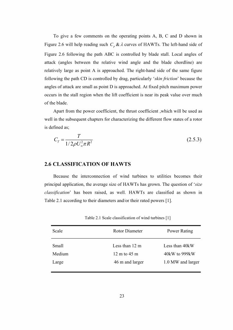
2.6 CLASSIFICATION OF HAWTS

Because the interconnection of wind turbines to utilities becomes their

principal application, the average size of HAWTs has grown. The question of ‘size

classification’ has been raised, as well. HAWTs are classified as shown in

Table 2.1 according to their diameters and/or their rated powers [1].

Table 2.1 Scale classification of wind turbines [1]

Scale Rotor Diameter Power Rating

Small Less than 12 m Less than 40kW

Medium 12 m to 45 m 40kW to 999kW

Large 46 m and larger 1.0 MW and larger

24

In Figure 2.7 scales of HAWTs are given for the prescribed rated capacity to

provide better understanding the relation between the rated capacity of a HAWT

with its rotor diameter and tower height.

Figure 2.7 Representative size, height and diameter of HAWTs [2]

2.7 CRITERIA IN HAWT DESIGN

Before ending this chapter, a few words to be mentioned in ref [8] about the

criteria in HAWT design and construction include:

• Number of turbine blades

• Rotor orientation; downwind or upwind rotor

• Turbine torque regulation

• Turbine speed; fixed or variable rotor speed

• Blade material, construction method and profile (airfoil section)

25

• Hub design; rigid, teetering or hinged

• Power control via aerodynamic control (stall control) or variable pitch

blades (pitch control)

• Orientation by self aligning action (free yaw) or direct control (active yaw)

• Types of mechanical transmission and generator; synchronous or induction

generator; gearbox or direct drive transmission

• Type of tower; steel or reinforced –concrete shell or steel truss with tension

cables

26

CHAPTER 3

AERODYNAMICS OF HAWTs

1.2 INTRODUCTION

Wind turbine power production depends on the interaction between the rotor

and the wind. The wind may be considered to be a combination of the mean wind

and turbulent fluctuations about that mean flow. Experience has shown that the

major aspects of wind turbine performance (mean power output and mean loads)

are determined by the aerodynamic forces generated by the mean wind. Periodic

aerodynamic forces caused by wind shear, off-axis winds, rotor rotation, randomly

fluctuating forces induced by turbulence and dynamic effects are the source of

fatigue loads and are a factor in the peak loads experience by a wind turbine. These

are, of course, important, but can only be understood once the aerodynamics of

steady state operation has been understood. Accordingly this chapter focuses

primarily on steady state aerodynamics.

The chapter starts with the analysis of an idealized wind turbine rotor. The

discussion introduces important concepts and illustrates the general behavior of

wind turbine rotors and the airflow around wind turbine rotors. The analysis is also

used to determine theoretical performance limits for wind turbines.

General aerodynamic concepts are then introduced. The details of momentum

theory and blade-element theory are developed. The combination of two theories,

called strip theory or blade-element momentum theory (BEM) is then studied to

outline the governing equations for the aerodynamic design and power prediction

of a wind turbine rotor which will be used in the next chapter.

The last section of this chapter discusses the vortex theory. Vortex theory is

another approach for aerodynamic design of wind turbine rotors, but here only its

27

concepts related to the former two theories are explained in order to make some

definitions in these theories more understandable.

1.2 THE ACTUATOR DISK THEORY AND THE BETZ LIMIT

A simple model, generally attributed to Betz (1926) can be used to determine

the power from an ideal turbine rotor, the thrust of the wind on the ideal rotor and

the effect of the rotor operation on the local wind field. The simplest aerodynamic

model of a HAWT is known as ‘actuator disk model’ in which the rotor becomes a

homogenous disk that removes energy from the wind. Actuator disk theory is based

on a linear momentum theory developed over 100 years ago to predict the

performance of ship propeller.

The theory of the ideal actuator disk is based on the following assumptions[9]:

• Homogenous, Incompressible, steady state fluid flow

• No frictional drag

• The pressure increment or thrust per unit area is constant over the disk

• The rotational component of the velocity in the slipstream is zero. Thus the

actuator disk is an ideal mechanism which imparts momentum to the fluid in the

axial direction only

• There is continuity of velocity through the disk

• An infinite number of blades

A complete physical representation of this actuator disk may be obtained by

considering a close pair of tandem propellers or turbine blades rotating in opposite

direction and so designed that the element of torque at any radial distance from the

axis has the same value for each blade in order that there shall be no rotational

motion in the slipstream; also each turbine actual blade must be replaced with its

small number of blades by another of the same diameter having a very large

28

U∞

p0 p0 pu pd

U3 U2 Uw

wake

actuator disk

Streamtubeboundary

number of very narrow equal frictionless blades, the solidity at any radius being the

same as for the actual turbine and finally to have the blade angles suitably chosen

to give a uniform distribution of thrust over the whole disk.

The analysis of the actuator disk theory assumes a control volume, in which

the control volume boundaries are the surface of a stream tube and two cross-

sections of the stream tube as shown in Figure 3.1.

1 2 3 4

Figure 3.1 Idealized flow through a wind turbine represented by a non-rotating,

actuator disk

The only flow is across the ends of the streamtube. The turbine is represented

by a uniform “actuator disk” which creates a discontinuity of pressure in the

streamtube of air flowing through it. Note also that this analysis is not limited to

any particular type of wind turbine.

From the assumption that the continuity of velocity through the disk exists;

2 3 RU U U= =

For steady state flow, air mass flow rate through the disk can be written as;

29

(3.1.1)Rm AUρ=i

Applying the conservation of linear momentum to the control volume

enclosing the whole system, the net force can be found on the contents of the

control volume. That force is equal and opposite to the thrust, T which is the force

of the wind on the wind turbine. Hence from the conservation of linear momentum

for a one-dimensional, incompressible, time-invariant flow the thrust is equal and

opposite to the change in momentum of air stream;

( ) (3.1.2)wT m U U∞= −i

No work is done on either side of the turbine rotor. Thus the Bernoulli function

can be used in the two control volumes on either side of the actuator disk. Between

the free-stream and upwind side of the rotor (from section 1 to 2 in Figure 3.1) and

between the downwind side of the rotor and far wake (from section 3 to 4 in Figure

3.1) respectively;

2 20

2 20

1 1 (3.1.3)2 21 1 (3.1.4)2 2

u R

d R w

p U p U

p U p U

ρ ρ

ρ ρ

∞+ = +

+ = +

The thrust can also be expressed as the net sum forces on each side of the

actuator disk;

(3.1.5)T Ap= ′

Where

( ) ( 3.1.6)u dp p p′ = −

By using equations 3.1.3 and 3.1.4, the pressure decrease, p′ can be found as;

30

( )2 21 (3.1.7)2 wp U Uρ ∞′ = −

And by substituting equation 3.1.7 into equation 3.1.5;

( )2 21 (3.1.8)2 wT A U Uρ ∞= −

By equating the thrust values from equation 3.1.2 in which substituting

equation 3.1.1 in place of mi

and equation 3.1.8, the velocity at the rotor plane can

be found as;

(3.1.9)2

wR

U UU ∞ +=

Thus, the wind velocity at the rotor plane, using this simple model, is the

average of the upstream and downstream wind speeds.

If an axial induction factor (or the retardation factor), a is defined as the

fractional decrease in the wind velocity between the free stream and the rotor plane,

then

( )( )

(3.1.10)

1 (3.1.11)

1 2

R

R

w

U UaU

U U a

U U a

∞

∞

∞

∞

−=

= −

= − (3.1.12)

The velocity and pressure distribution are illustrated in Figure 3.2. Because of

continuity, the diameter of flow field must increase as its velocity decreases and

note that there occurs sudden pressure drop at rotor plane which contributes the

torque rotating turbine blades.

31

Figure 3.2 Velocity and pressure distribution along streamtube

The power output, P is equal to the thrust times the velocity at the rotor plane;

RP TU=

Using equation 3.1.8,

( )2 212 w RP A U U Uρ ∞= −

And substituting for RU and wU from equations 3.1.11 and 3.1.12,

( )2 32 1 (3.1.12)P Aa a Uρ ∞= −

Using equation 2.5.1, the power coefficient pC becomes;

32

( )24 1 (3.1.13)pC a a= −

The maximum pC is determined by taking the derivative of equation 3.1.13

with respect to a and setting it equal to zero yields;

max( ) 16 / 27 0.5926pC = =

When 1/3a =

This result indicates that if an ideal rotor were designed and operated such that

the wind speed at the rotor were 2/3 of the free stream wind speed, then it would be

operating at the point of maximum power production. This is known as the Betz

limit.

From equations 3.1.8, 3.1.11 and 3.1.12 the axial thrust on the disk can be

written in the following form;

( ) 22 1 ) (3.1.14)T Aa a Uρ ∞= −

Similarly to the power coefficient, thrust coefficient can be found as by use of

equation 2.5.3;

4 (1 ) (3.1.15)TC a a= −

Note that TC has a maximum of 1.0 when 0.5a = and the downstream velocity

is zero. At maximum power output ( 1/ 3)a = , TC has a value of 8/9. A graph of the

power and thrust coefficients for an ideal Betz turbine is illustrated in Figure 3.3.

Note that, as it can be seen in Figure 3.3, this idealized model is not valid for

an axial induction factors greater than 0.5.

33

Figure 3.3 Operating parameters for a Betz turbine

In conclusion, the actuator disk theory provides a rational basis for illustrating

that the flow velocity at the rotor is different from the free-stream velocity. The

Betz limit ,max 0.593pC = shows the maximum theoretically possible rotor power

coefficient that can be attained from a wind turbine. In practice three effects lead to

a decrease in the maximum achievable power coefficient;

• Rotation of wake behind the rotor

• Finite number of blades and associated tip losses

• Non-zero aerodynamic drag

3.3 THE GENERAL MOMENTUM THEORY

The axial momentum theory of the previous section was developed on the

assumption that there was no rotational motion in the slipstream and that the

34

turbine blades could be replaced by an actuator disk which produced a sudden

decrease of pressure in the fluid without any change of velocity. More generally,

the slipstream will have a rotational motion by the reaction of the torque of the

blade and this rotational motion implies a further loss of energy. To extend the

theory to include the effects of this rotational motion, it is necessary to modify the

qualities of the actuator disk by assuming that it can also impart a rotational

component to the fluid velocity while the axial and radial components remain

unchanged.

Using a streamtube analysis, equations can be written that express the relation

between the wake velocities (both axial and rotational) and the corresponding wind

velocities at the rotor disk. In Figure 3.4 an annular streamtube model of this flow

illustrating the rotation of the wake is shown for making the visualization clear.

And Figure 3.5 illustrates the geometry of this streamtube model of wind flow

through a HAWT.

Figure 3.4 Streamtube model of flow behind rotating wind turbine blade

Rotor plane

35

Figure 3.5 Geometry of the streamtube model of flow through a HAWT rotor

Referring to the Figure 3.5, let r be the radial distance of any annular element

of the rotor plane, and let u and v be respectively the inflow (the flow immediately

in front of the rotor plane) axial and radial components of the fluid velocity. Let pu

be the inflow pressure and let p' be the decrease of outflow (the flow immediately

behind the rotor plane) pressure associated with an angular velocity w. In the final

wake let pw be the pressure, uw be the axial velocity and ww be the angular velocity

at a radial distance rw from the axis of the slipstream.

By applying the condition of continuity of flow for the annular element is;

(3.2.1)w w wu r dr urdr=

And the condition for constancy of angular momentum of the fluid as it passes

down the slipstream is;

2 2 (3.2.2)w ww r wr=

Also since the element of torque of the radial blade element is equal to the angular

momentum extracted in unit time to the corresponding annular element of the

slipstream;

U∞

p0 pw

pu pd

wake

Rotor plane

rrw

dr

uv

uv

w

uw

vw

free-stream

streamlines

36

2 (3.2.3)dQ uwr dAρ=

Where 2dA rdrπ=

For constructing the energy equation, Bernoulli’s equation can be used

separately from free-stream to inflow conditions and from outflow to wake

conditions;

( )

2

2 2

121 2

o o

u

H p U

p u v

ρ

ρ

∞= +

= + +

( )

( )

2 2 2 21

2 2 2

1 21 2

d

w w w w

H p u v w r

p u w r

ρ

ρ

= + + +

= + +

Hence

( )2 21

1 (3.2.4)2oH H p w rρ− = ′ −

Equation 3.2.4 shows that the decrease of total pressure head passing through

the blade element is below the thrust per unit area p′ by a term representing the

kinetic energy of the rotational motion imparted to the fluid by the torque of the

blade.

The expressions for the total pressure head also give;

( ) ( )

( ) ( )

2 2 2 20 1

2 2 2 2 2 2

1 12 21 1 (3.2.5)2 2

o w w w w

w w w

p p u U w r H H

u U w r w r p

ρ ρ

ρ ρ

∞

∞

− = − + + −

= − + − + ′

To find the pressure drop, p′ Bernoulli’s equation can be applied between

inflow and outflow relative to the blades which are rotating with an angular

37

velocityΩ . Note that the flow behind the rotor rotates in the opposite direction to

the rotor, in reaction to the torque exerted by the flow on the rotor. Hence the

angular velocity of the air relative to the blade increases from Ω to ( )wΩ + , while

the axial component of the velocity remains constant. The result is;

( )

( )

2 2 2

2

12

/ 2 (3.2.6)

p w r

w wr

ρ Ω Ω

ρ Ω

′ = + −

= +

Finally, combining this result (equation 3.2.6) with the previous equations

3.2.2 and 3.2.5, the drop of pressure in the wake becomes;

( ) ( )2 2 21 / 2 (3.2.7)2o w w w wp p u U w w rρ ρ Ω∞− = − + +

The pressure gradient in the wake balances the centrifugal force on the fluid

and is governed by the following equation;

2 (3.2.8)ww w

w

dp w rdr

ρ=

And then differentiating equation 3.2.7 relative to wr and equating to equation

3.2.8, a differential equation is obtained connecting the axial and rotational

velocities in the wake,

( ) ( )2 2 21 (3.2.9)2 w w w w

w w

d dU u w w rdr dr

Ω∞ − = +

The equation of axial momentum for the blade element, which can be

established rigorously by a simple extension of the analysis of the previous section,

( ) ( ) w w w o w wT u U u dA p p dAρ ∞= − + −∫ ∫

38

and in the differential form;

( ) ( ) (3.2.10)w w w o w wdT u U u dA p p dAρ ∞= − + −

also from the pressure decrease at the rotor plane, dT can alternatively be written

as;

(3.2.11)dT p dA= ′

By inserting equation 3.2.6 into its place in equation 3.2.11,

( ) 2/ 2 (3.2.12)dT w wr dAρ Ω= +

Finally, combining equation 3.2.1, 3.2.5, 3.2.10 and 3.2.12,

[ ]2 21 / 2 / 2 (3.2.13)2

ww w w w

w

w wU u u w ru U

Ω Ω∞

∞

+ +− = −

It should be emphasized that the equation of axial momentum is based on the

assumption that the axial force due to the pressure on the lateral boundary of the

streamline is equal to the pressure force, ( )o o w wp A p A− over its ends. This

assumption implies that the mutual interference between various annular elements

has been neglected but the actual deviations from the conditions represented by

equation 3.2.12 are believed to be extremely small in general. The other

assumptions made for deriving the general momentum equations so far are that the

rotor was treated as having very large number of very narrow blades (infinite

number of blades) resulting in negligible radial component of the velocity of the

fluid and the air is incompressible and inviscid, i.e., fluid drag is zero [10].

Equations 3.2.1, 3.2.2, 3.2.9 and 3.2.13, though rather complex in form, suffice

to determine the relationship between the thrust and torque of the blade and the

flow in the slipstream. If, for example, the angular velocity ww is known as a

39

function of the radius r in the wake, equation 3.2.9 determines the axial velocity,

wu and then equation 3.2.13, taken in conjunction with equation 3.2.1 and equation

3.2, determines the axial and rotational velocities at the rotor plane. The thrust and

torque of the rotor are then obtained from equation 3.2.12 and equation 3.2.3

respectively. Owing to the complexity of these equations, however, it is customary

to adopt certain approximations based on the fact that the rotational velocity in the

slipstream is generally very small.

An exact solution of the general momentum equations can be obtained when

the flow in the slipstream is irrotational except along the axis. This condition

implies that the rotational momentum 2wr has the same value for all radial

elements. Then by virtue of equation 3.2.11, the axial velocity, wu is constant along

a radius because this equation’s right-hand side is zero.

Defining the axial velocities u and wu as

( )( )1

1w

u U a

u U b∞

∞

= −

= −

After some algebraic manipulations, it can be obtained from equation 3.2.13,

( ) 2

2

11 (3.2.14)

2 4 ( )a bbab aλ

−= − −

Examination of equation 3.2.14 shows that the axial velocity reduction of the

rotor disk is always approximately one-half the reduction in the far-wake for the

tip-speed ratio above 2, which is the same result reached in the previous section

when the wake rotation was neglected.

For the approximate solution, the following assumption is made. The angular

velocity w imparted to the slipstream is very small compared with the angular

velocity Ω of the blades and it is therefore possible to simplify the general

40

equations by neglecting certain terms involving 2w [10]. On this basis of

approximation the pressure wp in the wake is equal to the initial pressure op of the

air and the decrease of pressure p′ across the rotor disk is equal to the decrease of

total pressure head 1( )oH H− . The relationships connecting the thrust and axial

velocity are then the same as in the simple momentum theory, the axial velocity u

at the rotor disk is the arithmetic mean of the axial velocity U∞ and the slipstream

velocity wu , and the element of thrust is

2

2 ( )

4 (1 ) (3.2.15)

dT u u U dA

U a a rdr

ρ

πρ∞

∞

= −

= −

Alternatively, from equation 3.2.6,

32 ( / 2)dT p dA

w wr drπρ Ω

= ′

= +

And defining angular induction factor, / 2a w Ω′ =

2 34 (1 ) (3.2.16) dT a a r drπρΩ= ′ + ′

Equating the two expressions for the thrust given in equation 3.2.15 and

equation 3.2.16, a relationship is obtained between axial induction factor, a and

angular induction factor a′ ,

2 22

2

(1 ) (3.2.17) (1 ) r

a a ra a U

Ω λ∞

−= =

′ + ′

The element of torque is obtained from equation 3.2.3 as following;

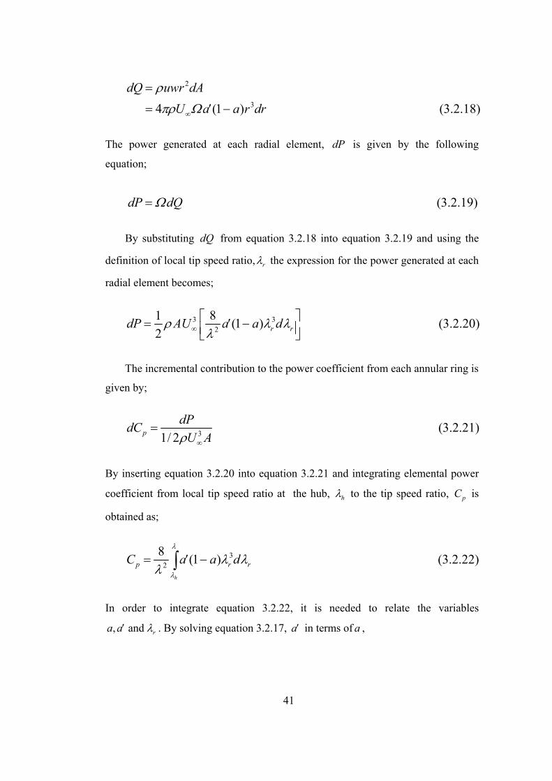
41

2

34 (1 ) (3.2.18)dQ uwr dA

U a a r drρ

πρ Ω∞

=

= ′ −

The power generated at each radial element, dP is given by the following

equation;

(3.2.19) dP dQΩ=

By substituting dQ from equation 3.2.18 into equation 3.2.19 and using the

definition of local tip speed ratio, rλ the expression for the power generated at each

radial element becomes;

3 32

1 8 (1 ) (3.2.20)2 r rdP AU a a dρ λ λ

λ∞ = ′ −

The incremental contribution to the power coefficient from each annular ring is

given by;

3 (3.2.21)1/ 2p

dPdCU Aρ ∞

=

By inserting equation 3.2.20 into equation 3.2.21 and integrating elemental power

coefficient from local tip speed ratio at the hub, hλ to the tip speed ratio, pC is

obtained as;

32

8 (1 ) (3.2.22)h

p r rC a a dλ

λ

λ λλ

= ′ −∫

In order to integrate equation 3.2.22, it is needed to relate the variables

, and ra a λ′ . By solving equation 3.2.17, a′ in terms of a ,

42

2

1 1 41 (1 ) (3.2.23)2 2 r

a a aλ

′ = − + + −

The aerodynamic conditions for the maximum possible power production

occur when the term (1 )a a′ − in equation 3.2.22 is at its greatest value.

Substituting the value for a′ from equation 3.2.23 into the term (1 )a a′ − and

setting the derivative with respect to a and equating to zero yields;

2

2 (1 )(4 1) (3.2.24)(1 3 )ra a

aλ − −

=−

And substituting equation 3.2.24 into equation 3.2.17, it is found that for maximum

power in each annular ring,

(1 3 ) /(4 1) (3.2.25)a a a′ = − −

If equation 3.2.24 is differentiated with respect to a , a relationship between rdλ

and da at those conditions is obtained;

2 22 6(4 1)(1 2 ) /(1 3 ) (3.2.26)r rd a a a daλ λ = − − −

Now, substituting the equations 3.2.24, 3.2.25 and 3.2.26 into the equation 3.2.22

gives;

2

1

2

,max 2

24 (1 )(1 2 )(1 4 ) (3.2.27)(1 3 )

a

pa

a a aC daaλ

− − −= −

∫

Where 1a : corresponding axial induction factor for r hλ λ=

2a : corresponding axial induction factor for rλ λ=

Also from equation 3.2.24;

43

22 2 2(1 )(1 4 ) /(1 3 ) (3.2.28)a a aλ = − − −

Equation 3.2.28 can be solved for the values of a that correspond to operation

at tip speed ratios of interest. Note also from equation 3.2.28, 2 1/ 3a = is the upper

limit of the axial induction factor giving an infinitely large tip speed ratio.

Table 3.1 presents a summary of numerical values for ,maxpC as a function of

rλ with corresponding values for the axial induction factor at the tip, 2a

Table 3.1 Power coefficient, ,maxpC as a function of tip-speed ratio, λ and 2a

λ 2a ,maxpC

0.5 0.2983 0.289

1.0 0.3170 0.416

1.5 0.3245 0.477

2.0 0.3279 0.511

2.5 0.3297 0.533

5.0 0.3324 0.570

7.5 0.3329 0.581

10.0 0.3330 0.585

The result of general momentum theory are graphically represented in Figure

3.6 which also shows the Betz limit of an ideal turbine based on the linear

momentum analysis performed in the previous section. The result shows that the

higher the tip-speed ratio, the greater the maximum power coefficient.

44

Figure 3.6 Theoretical maximum power coefficients as a function of tip-speed ratio

for an ideal HAWT with and without wake rotation

3.4 BLADE-ELEMENT THEORY

The momentum theories, which have been developed in the previous sections,

are based on a consideration of the mean axial and rotational velocity in the

slipstream and determine the thrust and torque of a blade from the rate of decrease

of momentum of the fluid. The theories determine an upper limit to the power

coefficient of any blade, depending on the free-stream wind velocity and on the

power extracted, but they restrict the understanding of the effect of rotor geometry

(i.e. blade airfoil section, chord and twist). The blade-element theory is an

alternative method of analyzing the behavior of blades due to their motion through

air.

As shown in Figure 3.7, for this analysis, it is assumed that the blade is

divided into N sections (or elements) and the aerodynamic force acting on each

blade element can be estimated as the force on suitable airfoil characteristics of the

same cross-section adopted for the blade elements. Finally assuming that the

behavior of each element is not affected by the adjacent elements of the same

45

blade, the force on the whole blade can be derived by adding the contributions of

all the elements along the blade.

Figure 3.7 Schematic of blade elements

A diagram showing the developed blade element at radius r and the velocities

and forces acting on this element is given in Figure 3.8.

The relative wind velocity relU is the vector sum of the wind velocity at the

rotor (1 )U a∞ − (the vector sum of the free-stream wind velocity, U∞ and the

induced axial velocity aU∞− ) and the wind velocity due to rotation of the blade.

And this rotational component is the vector sum of the blade section velocity, rΩ

and the induced angular velocity a rΩ′ . Hence the relative wind velocity will be as

shown on the velocity diagram in Figure 3.8. The minus sign in the term (1 )U a∞ −

is due to the retardation of flow while the air approaching the rotor and the plus

sign in the term (1 )r aΩ + ′ as shown in Figure 3.8 is due to the flow of air in the

reverse direction of blade rotation after air particles hit the blades and so give

torque.

In the mean time let the existence of the axial and angular induction factors

assumed, their evaluation will be given in the subsequent section.

46

Figure 3.8 Blade Geometry for analysis of a HAWT

From Figure 3.8 the following relationships can be determined;

(1 ) (3.3.1)sin( )rel

U aUϕ

∞ −=

(1 ) (1 ) tan( ) (3.3.2)(1 ) (1 ) r

U a ar a a

ϕΩ λ

∞ − −= =

+ ′ + ′

21 (3.3.3)2D D reldF C U cdrρ=

47

21 (3.3.4) 2L L reldF C U cdrρ=

cos sin (3.3.5)L DdT dF dFϕ ϕ= +

sin cos (3.3.6)L DdL dF dFϕ ϕ= −

If the rotor has B number of blades, the total normal and tangential force on

the element at a distance r by rearranging equation 3.3.5 and 3.3.6 with the use of

equation 3.3.1, 3.3.3 and 3.3.4;

21 ( cos sin ) (3.3.7)2 rel L DdT B U C C cdrρ ϕ ϕ= +

21 ( sin cos ) (3.3.8)2 rel L DdL B U C C cdrρ ϕ ϕ= −

The elemental torque due to the tangential forces, dL operating at a distance r

from the center is given by;

(3.3.9)dQ rdL=

hence the elemental torque by inserting equation 3.3.8 into equation 3.3.9;

21 ( sin cos ) (3.3.10)2 rel L DdQ B U C C crdrρ ϕ ϕ= −

From the velocity diagram in Figure 3.8, relative wind velocity can be written

as below;

48

(1 ) (3.3.11)sinrel

U aUϕ

∞ −=

and by defining solidity ratio, σ as following;

(3.3.12)2Bc

rσ

π=

and inserting equations 3.3.11 and 3.3.12 into equations 3.3.7 and 3.3.10, the

general form of elemental thrust and torque equations become;

2 2

2

(1 ) ( cos sin ) (3.3.13)sin L D

U adT C C rdrσπρ ϕ ϕϕ

∞ −= −

2 22

2

(1 ) ( sin cos ) (3.3.14)sin L D

U adQ C C r drσπρ ϕ ϕϕ

∞ −= −

Thus, from blade element theory, two equations (3.3.13 and 3.3.14) have been

obtained. They define the normal force (thrust) and the tangential force (torque) on

an annular rotor section as a function of the flow angles at the blades and airfoil

characteristics.

Here it is convenient to consider in turn the following assumptions which are

the bases of developing blade element theory [11]:

• The assumption that the behavior of an element is not affected by the

adjacent elements of the same blade

• The airfoil characteristics to be adopted for the element

49

The independence of blade elements, assumed in the blade element theory and

also in all later developments of theory, is analogous to the assumption adopted in

the general momentum theory that the thrust on an elementary annulus of a rotor

may be expressed as 2 ( )dT u u U dAρ ∞= − (equation 3.2.15). In the discussion of

general momentum theory it was pointed out that this equation could not be

established rigorously. Similarly, in the blade element theory, it is not possible to

give a rigorous proof of the independence of the blade elements and the validity of

the assumption must be justified by an appeal to suitable experimental results. If

the assumption valid, the thrust on the blade element at radial distance r with the

blade angle θ should be independent of the variation of the blade angle along the

remainder of the blade. A check of the assumption can therefore be obtained by

taking two propellers of different pitch with blades of the same plan form and

section and by rotating the blades of one rotor so that the blade angles of the two

rotors have the same value at a chosen radial distance r . The thrust distribution

along the blades should then show the same element of thrust on the blade elements

under examination. By means of a series of experiments [12] has been established

the independence of the blade elements over the principal part of the blades.

The second assumption states that two-dimensional airfoil characteristics can

be used for the blade elements. Airfoil two-dimensional characteristics are usually

determined from tests of a rectangular airfoil of different aspect ratio. Hence the lift

and drag characteristics are dependent on aspect ratio. But in the fully-attached

regime, airfoil section characteristics are not generally affected by aspect ratio, and

since HAWT rotors operate in the fully-attached regime of the flow while

extracting maximum energy from the wind, two-dimensional (i.e. infinite aspect

ratio) can be used in predicting performance. However, when two-dimensional data

are used, a tip-loss factor must be added as will be described in the next chapter.

50

3.5 BLADE ELEMENT-MOMENTUM (BEM) THEORY

In the general momentum theory attention was directed to the motion of the

fluid and the forces acting on the blades were determined. The defect of the general

momentum theory was that it gave no indication of the shape of blade required to

produce the reactions considered.

The principle of the blade element theory was to consider the forces

experienced by the blades of the rotor in their motion through the air and this

theory was therefore intimately concerned with the geometrical shape of the blade.

In order to bridge the gap between these two theories, the blade element

momentum theory (BEM) which is also known as strip theory has been developed.

BEM theory relates rotor performance to rotor geometry and particularly important

prediction of this theory is the effect of finite blade number.

The assumptions for BEM theory are obviously the combination of those

which were made for general momentum and blade element theory. The foremost

assumption in BEM theory is that individual streamtubes (the intersection of a

streamtube and the surface swept by the blades) can be analyzed independently of

the rest of the flow as assumed before for the blade element theory.

A second assumption associated with the development of BEM theory is that

spanwise flow is negligible, and therefore airfoil data taken from two-dimensional

section tests are acceptable as assumed before in again blade element theory.

A third assumption is that flow conditions do not vary in the circumferential

direction, i.e. axisymmetric flow. With this assumption the streamtube to be

analyzed is a uniform annular ring centered on the axis of revolution as assumed

before in general momentum theory.

BEM theory refers to the determination of a wind turbine blade performance

by combining the equations of general momentum theory and blade element

51

theory. In this case by equating the elemental thrust force equations from general

momentum theory and blade element theory (equations 3.2.15 and 3.3.13

respectively) the following relationship is obtained;

[ ]2

cos( ) 1 ( ) tan (3.4.1)(1 ) 4sinL D L

a C C Ca

ϕσ ϕϕ

= +−

and equating the elemental torque derived in both general momentum theory and

blade element theory (equations 3.2.18 and 3.3.14 respectively);

[ ]( ) 1 ( )cot (3.4.2)(1 ) 4 sin

LD L

r

a C C Ca

σ ϕλ ϕ

′= −

−

Equation 3.4.2 can be rearranged by using equation 3.3.2, which relates

, , and ra a ϕ λ′ based on the geometric considerations;

[ ]( ) 1 ( )cot (3.4.3)(1 ) 4cos

LD L

a C C Ca

σ ϕϕ

′= −

+ ′

In the calculation of induction factors and a a′ , accepted practice is to set DC

zero for the purpose of determining induction factors independently from airfoil

characteristics. For airfoils with low drag coefficient, this simplification introduces

negligible errors [13]. So equation 3.4.1, 3.4.2 and 3.4.3 can be rewritten

considering 0DC ≈

2

cos( ) (3.4.4)(1 ) 4sinL

a Ca

ϕσϕ

=−

52

( ) (3.4.5)(1 ) 4 sin

L

r

a Ca

σλ ϕ

′=

−

( ) (3.4.6)(1 ) 4cos

La Ca

σϕ

′=

+ ′

By using these three equations the following useful relationships result after some

algebraic manipulation;

4sin (cos sin ) (3.4.7)(sin cos )

rL

r

C ϕ ϕ λ ϕσ ϕ λ ϕ

−=

+

2

1 (3.4.8)1 [4sin ( )cos ]L

aCϕ σ ϕ

= +

[ ]1 (3.4.9)

[4cos ( )] 1L

aCϕ σ

′ =−

tan (3.4.10)ra a λ ϕ′ =

To determine the power coefficient of a wind turbine, the power contribution

from each annulus is found firstly, then integrated along the blade length and

finally using the equation 2.5.1, power coefficient pC can be obtained.

The elemental power from each blade element was defined in equation 3.2.19

as;

(3.2.19)dP dQΩ=

53

And the total power from the rotor is;

(3.2.20)h h

R R

r r

P dP dQΩ= =∫ ∫

Hence the power coefficient pC becomes by rewriting equation 2.5.1 here,

3 3 2 (3.4.11)1/ 2 1/ 2

h

R

rp

dQPCU A U R

Ω

ρ ρ π∞ ∞

= =∫

Using the expression for the elemental torque from equation 3.3.14, the power

coefficient can be expressed as below,

[ ]2

22

2 (1 ) 1 ( )cot (3.4.12)sinp L D L r r

aC C C C dσ ϕ λ λλ ϕ

−= −∫

Finally by using equations 3.4.4 and 3.4.10 in equation 3.4.12, the general form of

power coefficient expression can be obtained as;

[ ]32

8 (1 ) 1 ( )cot (3.4.13)h

p r D L rC a a C C dλ

λ

λ ϕ λλ

= ′ − −∫

Note that when 0DC ≈ , the equation above for pC is the same as the one

derived from the general momentum theory (equation 3.2.22).

An alternative expression for the power coefficient can be derived after

performing the tedious algebra and by inserting equations 3.4.7 and 3.4.8 into

equation 3.4.12;

54

( )( ) ( )2

2 2

sin cos sin sin cos 1 cot ...8 (3.4.14)

h

r r D Lp

r r

C CC

d

λ

λ

ϕ ϕ λ ϕ ϕ λ ϕ ϕλ λ λ

− + − = ∫

Note that even though the axial and angular induction factors were determined

assuming the 0DC = , the drag is included in the power coefficient calculation.

By the same token, the thrust coefficient TC can be found beginning from the

definition of thrust coefficient in the equation 2.5.3 as following;

( )( ) ( )2

sin 2 cos sin sin cos 1 tan ...4 (3.4.15)

h

r r D LT

r r

C CC

d

λ

λ

ϕ ϕ λ ϕ ϕ λ ϕ ϕλ λ λ

− + + = ∫

3.6 VORTEX THEORY

In addition to BEM theory which will be used for rotor performance analysis

and blade design of HAWT in this thesis; vortex theory is an alternative theory

which provides a method of analyzing the rotor performance. Even though vortex

theory is not the scope of this thesis there is a necessity of discussing of this theory

briefly without going into its detail. Because the vortex theory explains the origin

of axial and angular induction factors which have been already introduced in both

general momentum theory and blade element theory without giving any physical

meaning about their existence.

The vortex theory depends fundamentally on the conception that the lift of an

airfoil section is associated with a circulation of the flow around its contour.

According to modern airfoil theory the lift L per unit length of an airfoil section in

two-dimensional motion is related to the circulation Γ around its contour by the

following equation;

55

(3.5.1)L Uρ Γ=

Applying this concept of airfoil theory to the problem of the rotor blades, it is

evident that there must be circulation of the flow around the blades of the rotor in

order to produce the aerodynamic force experienced by the blades. In general the

circulation Γ around the blade element will vary along the blade, but to explain

the mode of action of the blades it is simpler to assume as a first step that the

circulation is constant along the whole blade. The existence of this circulation can

be expressed also by the statement that there is a vortex line of strengthΓ , bound

to the blade and running along it from root to tip. But a vortex line can not begin or

end abruptly; unless it forms a closed curve in the body, it must be continued as a

free vortex line in the fluid and in this latter form it follows the general motion of

the fluid as a trailing vortex behind the body. Thus the bound vortex must be

continued by two free vortices in the fluid, one springing from the root of the blade

and the other from its tip. As shown in Figure 3.9 the free vortex springing from

the roots of propeller blades will be straight line along the axis of the propeller and

its strength will be BΓ for a propeller with B blades. The tip vortices, each of

strengthΓ , will be of helical shape and will be tracing out the paths described by

the tips of the propeller blades.

Figure 3.9 Tip and root vortices

56

Up to this point the vortex system of a rotor or propeller has been based for

simplicity on the assumption that the circulation along the blade is constant. More

generally, however, the strength of the circulation will vary along the blade and

indeed the condition of constant circulation along the whole blade is physically

impossible. Because the pressure difference between the top and bottom surface of

the blade causes flow and pressure equalization near the blade tips. For an

illustration the actual variation of the circulation along the blade is given in

Figure 3.10. Due to the variation of the circulation along the blade, trailing vortices

will arise, not only at the root and tip of the blade, but from every point of its

trailing edge, forming a continual screwlike vortex sheet.

Figure 3.10 Variation of bound circulation along blade length

If δΓ is the increase of circulation between the points and ( )r r rδ+ of the

blade, then the strength of the helical vortex springing from this element will be

δΓ− . The vortex line springing from one blade form a vortex sheet in the form of

a screw surface and there will be one such surface for each blade. The slipstream of

the rotor consists of these vortex sheets and of the fluid contained between them.

57

The disturbance of the flow caused by a rotor can be represented as the

induced velocity of the completed vortex system, comprising the bound vortices of

the propeller blades and the free vortex sheets of the slipstream and the motion of

the fluid relative to the propeller is the resultant of the axial velocity and its

induced velocity.

Owing to the difficulty of calculating the induced velocity of the system of

helical vortex sheets which constitute the slipstream of a rotor, the induced velocity

is usually calculated on the assumption that the propeller has a very large number

of blades. This assumption implies that the vorticity of the slipstream is distributed

throughout the whole of the fluid instead of being concentrated on a few vortex

sheets and the vorticity can then be assumed to be grouped in the following

manner. Considering first the condition of constant circulation along the blades, the

boundary of the slipstream is a cylindrical vortex sheet as shown in Figure 3.11.

Figure 3.11 Helical vortices replaced by axial and circumferential vortex lines

In place of the helical vortex lines covering the surface, the vorticity of the

sheet may be considered a close succession of vortex rings RR whose vorticity

represents the decreased axial velocity of the slipstream and a surface of vortex

58

lines LL whose vorticity represents the rotation of the slipstream. The vortex

system is completed by the axial vortex AA. More generally, with circulation

varying along the blades of the propeller, the whole slipstream must be considered

as full of vortex systems of this simpler type.

The induced velocity of the vortex system in the ultimate wake far behind the

rotor plane will be an axial velocity ( )wU u∞ − and an angular velocity ww , which

will be function of the radial coordinate wr . In this wake the induced velocity of the

bound vortices of the blades is negligibly small. At the disc also the bound vortices

can not give any component to the axial velocity owing to the symmetrical

distribution of this vorticity relative to any arbitrary point of the disc and hence the

axial induced velocity ( )u U∞− will be due wholly to the trailing vortex system.

Also if the expansion of the slipstream can be ignored in calculating these

induced velocities, it can easily be seen that the axial induced velocity at the rotor

disk is half that in the ultimate wake; for the vortex system is then simply a long

cylinder extending indefinitely in one direction from the rotor disk and the induced

axial velocity at a point of the wake, where the cylinder extends indefinitely in both

directions, must clearly be double that at the corresponding point of the rotor disk.

Thus

1( ) ( )2 wU u U u∞ ∞− = −

Or

1 ( ) (3.1.8)2 wu U u∞= +

which is the well known equation of the momentum theory described in section 3.1

from which the axial induction factor has been defined.

59

The induced angular velocity w immediately behind the rotor disk can be

related to the corresponding angular velocity ww in the wake by considering the

constancy of circulation of the fluid. The ring of fluid of radius r immediately

behind the rotor disk has the circulation 22 wrπ and by the laws of hydrodynamics

this circulation must remain constant as the ring of fluid passes down stream. In the

wake the radius of the ring has expanded to wr and there must therefore be a

decrease of the angular velocity governed by the equation as described in section

3.2;

2 2 (3.2.2)w wwr w r=

Immediately in front of the rotor disk there can be no such circulation, since

the fluid approaching the rotor is in irrotational motion. Also the bound vorticitiy

of the rotor blades must cause equal and opposite induced angular velocities w± ′

immediately before and behind the rotor disk and hence the induced angular

velocity of the trailing vortex system must have the value w′ at the rotor disk in

order to cancel the effect of the bound vortices in front of the disk. It follows that

the total induced angular velocity immediately behind the rotor disk is 2w′ and this

is the angular velocity previously denoted by w . Hence the induced angular

velocity of the trailing vortices at the propeller disk is 12

w and the angular

induction factor in section 3.2 has been defined by taking this value as a basis.

Vortex theory shows also the independence of blade elements which has been

assumed in blade element theory in section 3.3 and tried to explained physically.

Here it will be explained with the help of vortex theory as well by taking the

consideration of the system of trailing vortices which leads to the conclusion that

induced flow experienced by the blade elements at radial distance r from the axis

depends solely on the forces experienced by these elements and is not influenced

by the blade elements at greater or less radial distance. Consider the action of the

60

blade elements dr at radial distance r when the remainder of each rotor blade is

inoperative. The trailing vortices which spring from the ends of the element lie on

the surfaces of two circular cylinders of radius and r r dr+ respectively and the

vorticity may be resolved into two components as described before; one having its

axis parallel to the rotor axis and the other being circumferential and similar to a

succession of vortex rings. The first component of the vorticity acts as the roller

bearings between the rotating shell of air bounded by the cylindrical surfaces and

the general mass of air. Now the general mass of air can not acquire any circulation

about the axis and hence the rotation due to the torque of the blade elements is

confined to the region between the two cylindrical surfaces. Hence also the

rotational interference due to the vortex system is experienced by those blade

elements which gave rise to the vorticity.

A similar argument can be applied to the second component of the vorticity

and thus the independence of the blade elements at different radial distances from

the axis of the rotor is established [14].

It may be summarized the results of the vortex theory as follows:

• The induced flow at any radius r depends only on the thrust and torque

grading at this radius. In other words, the blade elements at differing radii are

hydrodynamically independent. This proves the validity of the assumption about

this result mentioned in blade element theory in section 3.3

• The induced axial velocity at a blade element is just half the axial velocity

in the distant part of the slipstream which comes from the element at that radius.

This is in agreement with the findings of the actuator disk theory of section 3.1

• The induced circumferential or rotational velocity of inflow at a blade

element is just the half the rotational velocity in the distant part of the slipstream

which comes from the elements at that radius which is what was done while

defining angular induction factor in the general momentum theory in section 3.2.

61

Before closing this section a few words about the advantages and

disadvantages of the vortex theory over the BEM theory are the following; the

BEM theory offers the method of ease of understanding and use as well as minimal

computation requirements. However there are a number of situations where it is not

reasonable to expect BEM methods over the vortex methods since vortex methods

offer the greatest accuracy. Though methods are available for incorporating some

complex effects such as yawed flow and unsteady aerodynamics into a BEM

analysis, it is much more desirable to seek analytical methods of vortex theory

which are fundamentally better suited to complex flows. The greatest obstacle to

widespread use of vortex methods is the computation burden. No programs are

currently available that calculate the details of an unsteady, three-dimensional, free

wake in a reasonable time, regardless of computer platform [7].

62

CHAPTER 4

HAWT BLADE DESIGN

1.2 INTRODUCTION

In this chapter, the application of BEM theory on the HAWT blade design and

analyzing the aerodynamic performance of a rotor will be explained.

BEM theory, as previously developed, does not account the effect of blade

numbers of a rotor. In other words, the equations of BEM theory were derived

assuming infinite number of blades of a rotor. This chapter begins with introducing

the concept of tip-loss factor and the generally recommended expression for

including tip losses in HAWT blade design is given. The governing equations

developed in BEM theory will then be modified in order to take the tip losses into

account.

In the next section flow states in which HAWTs are operating will be

examined. At which values of axial induction factor the application of BEM theory

becomes invalid will be explained and the Glauert empirical relationship will then

be given in order to proceed the blade design for those values of axial induction

factor.

Since the HAWT blades are made from airfoils to transform the kinetic energy

in the wind into useful energy, subsequent section is left to the introduction of

airfoil selection criteria in HAWT blade design. Most used airfoil families are

described as well.

After giving all these necessary knowledge for a blade design, the blade design

procedure for an optimum rotor and power performance prediction procedure for

the modified blade shape are given. The output of the BLADESIGN program

performed for the airfoil NACA 4412 are also put in this section as an example.

63

The chapter is ended with the results and explanatory figures showing the

effect of some parameters relating to the blade design.

It should be noted here that various methods [15,16,17,18,19] for HAWT

blade design and predicting performance of a rotor have been studied and the

important concepts [20,21] for design procedure have been used while developing

the user-interface computer program, BLADESIGN.

1.2 THE TIP-LOSS FACTOR

There was an assumption; the rotor has an infinite number of blades which

was used in all theories discussed in the previous chapter. With the aid of this

assumption radial velocity of the flow across the rotor plane and in the wake has

been always neglected and by so the derivations of governing equations have been

established. But near the boundary of the slipstream the air tends to flow around the

edges of the blade tips and acquires an important radial velocity. Because the

pressure on the suction side of a blade is lower than on the pressure side which

causes the air to flow around the tip from the lower to upper surface, reducing lift

and hence power production near the tip.

A number of methods have been suggested for including the effect of tip

losses. An approximate method of estimating the effect of this radial flow and

hence including the effect of tip losses has been given by L.Prandtl. Prandtl tip loss

model is generally recommended for the following reasons;

• Prandtl model prediction are in qualitative agreement with the behavior of

HAWT rotors,

• Calculations of rotor power and thrust made with Prandtl model are in good

agreement with test data,

• BEM theory calculations made with Prandtl model show good agreement

with calculations made with vortex theory,

64

• The Prandtl model is easier to program and use

The expression obtained by Prandtl for tip-loss factor is given by the following

equation [22];

( ) ( ) ( )( )

1 / 2 12 cos exp (4.2.1)

sinB r R

Fr R

πϕ

− − − =

The application of this equation for the losses at the blade tips is to provide an

approximate correction to the system of equations summarized in section 3.4.2 for

predicting rotor performance and blade design.

The physical fact represented by the tip correction is virtually that the

maximum decrease of axial velocity ( )wU u∞ − or 2aU∞ in the slipstream occurs

only on the vortex sheets and that the average decrease of axial velocity in the

slipstream is only a fraction F of this velocity. Thus, to order of approximation of

the analysis the correct form of the axial momentum equation (equation 3.2.15)

will be taken to be [2];

24 (1 ) (4.2.2)dT F U a a rdrπρ ∞= −

Similarly, also the angular momentum equation (equation 3.2.18) will be

assumed to be [2];

34 (1 ) (4.2.3) dQ F U a a r drπρ Ω∞= ′ −

Thus the effect of the tip-loss is to reduce slightly the thrust and torque

contributed by the elements near the tips of the blades.

Equations derived in section 3.3 are all based on the definition of the forces

used in blade element theory and remain unchanged. When the forces from the

65

general momentum theory are set equal using the method of BEM theory as

performed before, the derivation of the flow condition is changed.

Carrying the tip-loss factor through the calculations, the changes (through

equations 3.4.4 to 3.4.9 and 3.4.14) will be as following;

2

cos( ) (4.2.4) (1 ) 4 sinL

a Ca F

ϕσϕ

=−

( ) (4.2.5)(1 ) 4 sin

L

r

a Ca F

σλ ϕ

′=

−

( ) (4.2.6)(1 ) 4 cos

La Ca F

σϕ

′=

+ ′

4 sin (cos sin ) (4.2.7)(sin cos )

rL

r

FC ϕ ϕ λ ϕσ ϕ λ ϕ

−=

+

2

1 (4.2.8) 1 [4 sin ( )cos ]L

aF Cϕ σ ϕ

= +

[ ]1 (4.2.9)

[4 cos ( )] 1l

aF Cϕ σ

′ =−

( )( ) ( )2

2 2

sin cos sin sin cos 1 cot ...8

(4.2.10)h

r r D Lp

r r

F C CC

d

λ

λ

ϕ ϕ λ ϕ ϕ λ ϕ ϕλ λ λ

− + − = ∫

66

Even though the tip-loss factor has been accounted for the development of the

computer program of the blade design and power performance prediction in this

thesis, for the purpose of simplifying the calculations without including the tip-loss

factor, an effective-radius of the rotor may be defined for the diminished thrust and

torque output of the tip regions. This effective radius is generally taken as about

3% smaller than the tip radius. Note that from equation 4.2.1 it can be seen that F

is always between 0 and 1 and in this empirical approach the following definition

can be set;

e

1 if 00 if r0.97

e

e

F r rF r Rr R

== ≤ ≤

≈

< <

4.3 HAWT FLOW STATES

Measured wind turbine performance closely approximates the results of BEM

theory at low values of the axial induction factors but general momentum theory is

no longer valid at axial induction factors greater that 0.5, because according to the

equation 3.1.10, the wind velocity in the far wake would be negative. In practice, as

the axial induction factor increases above 0.5, the flow patterns through the wind

turbine become much more complex than those predicted by the general

momentum theory.

The thrust coefficient represented by the equation 3.1.14 can be used to

characterize the different flow states of a rotor. Figure 4.1 shows flow states and

thrust force vectors T associated with a wide range of axial induction factors.

According to this figure, for negative induction factors ( )0a < it is simple to

continue the analysis to show that the device will act as a propulsor producing an

upwind force (i.e. 0TC < ) that adds energy to the wake. This is typical of the

propeller state. The operating states relevant to HAWTs are designated by the

windmill state and the turbulent wake state. The windmill state is the normal

67

operating state. The windmill state is characterized by the flow conditions

described by general momentum theory for axial induction factors less than about

0.5. As illustrated by the data in Figure 4.1 obtained on wind turbines, above

a =0.5, rotor thrust increases up to 2 with increasing induction factor in the

turbulent wake state, instead of decreasing as predicted by the equation 3.1.14.

While general momentum theory no longer describes the turbine behavior,

Glauert’s empirical formula for axial induction factor from 0.4 to 1.0 are often used

in HAWT rotor design for predicting wind turbine flow states.

Figure 4.1 Relationship between the axial induction factor, flow state and thrust of a

rotor[1]

Windmill state Turbulent Wake state

4 (1 )TC a a= −

68

When the induction somewhat over unity, the flow regime is called the vortex

ring state and when a >2.0 the rotor reverses the direction of flow which is termed

propeller brake state with power being added to flow to create downwind thrust on

the rotor.

In the turbulent wake state, as stated before, a solution can be found by using

the Glauert empirical relationship between the axial induction factor, a and the

thrust coefficient, TC in conjunction with the blade element theory. The empirical

relationship developed by Glauert, including tip losses is [2];

( ) ( )1 0.143 0.0203 0.6427 0.889 (4.3.1)Ta F C = + − −

This equation is valid for 0.4a > or equivalently for 0.96TC >

The Glauert empirical relationship was determined for the overall thrust

coefficient for a rotor. It is customary, however, to assume that it applies equally to

equivalently local thrust coefficients for each blade section. The local thrust

coefficient rTC can be defined for each annular rotor section as;

2 (4.3.2)1/ 2 2rT

dTCU rdrρ π∞

=

From the equation 3.3.13 for the elemental thrust force from blade element theory,

the local thrust coefficient becomes;

( ) ( )2 21 cos sin sin (4.3.3)rT L DC a C Cσ ϕ ϕ ϕ= − +

In order to include the blade design and power performance prediction of

highly loaded HAWTs which are operating at high tip-speed ratios, the Glauert

empirical formula is used in the developing of the computer program. It firstly

69

calculates the local thrust coefficient for each blade section according to the

equation 4.3.3 and if 0.96rTC < then uses the previously derived equations for the

blade design. If 0.96rTC > then it estimates axial induction factor using equation

4.3.1 and this new value of axial induction factor is used in the equations for the

design.

4.4 AIRFOIL SELECTION IN HAWT BLADE DESIGN

HAWT blades use airfoils to develop mechanical power. The cross-sections of

HAWT blades have the shape of airfoils. The width and length of the blade are

functions of the desired aerodynamic performance, the maximum desired rotor

power, the assumed airfoil parameters and strength calculations. Hence designing

HAWT blade depends on knowledge of the properties of airfoils.

The most significant flow factor influencing the behavior of airfoils is that of

viscosity which is characterized by the Reynolds number of the airfoil/fluid

combination. The Reynolds number Re is defined by:

Re (4.4.1)relU cυ

=

Airfoils in use on modern wind turbines range in representative chord size

from about 0.3 m on a small-scale turbine over 2 m on a megawatt-scale rotor. Tip

speeds typically range from approximately 45 to 90 m/s. Then for HAWT airfoils

Reynolds number range from about 0.5 million to 10 million. This implies that

turbine airfoils generally operate beyond sensitive.

It should be noted that there are significant differences in airfoil behavior at

different Reynolds numbers. For that reason it must be made sure that appropriate

Reynolds number data are available for the blade design.

70

The lift and drag characteristics of airfoils show also significant aspect-ratio

dependence at angles of attack larger than 30 deg. But in the fully-attached region

in which HAWT is operating under windmill state are not greatly affected by

aspect-ratio, so that two-dimensional (i.e. infinite aspect-ratio) data can be used in

blade design at low angles of attack. However, when two-dimensional data are

used, tip-loss factor must be added as described in equation 4.2.1.

In this thesis what has been considered in constructing the airfoil database

from the computer program XFOIL which will be mentioned in the next chapter

includes these considerations; two-dimensional data with Reynolds number in the

order of 1 million.

There are evidently many engineering requirements into the selection of a

wind turbine airfoil. These include primary requirements related to aerodynamic

performance, structural, strength and stiffness, manufacturability and

maintainability.

The usual assumption is that high lift and low drag are desirable for an airfoil

and that the drag-to-lift ratio γ which is known as glide ratio as given below is a

critical consideration [23];

/ (4.4.2)D LC Cγ =

Airfoils for HAWTs are often designed to be used at low angles of attack,

where lift coefficients are fairly high and drag coefficients are fairly low(i.e. fairly

low glide ratio). Many different standard airfoils developed for aircraft have been

used on HAWTs. The NACA 230XX series and NACA44XX series airfoils have

been used on many modern HAWT units. The NACA 63-2XX series airfoils have

demonstrated the best overall performance characteristics of the NACA airfoil

families.

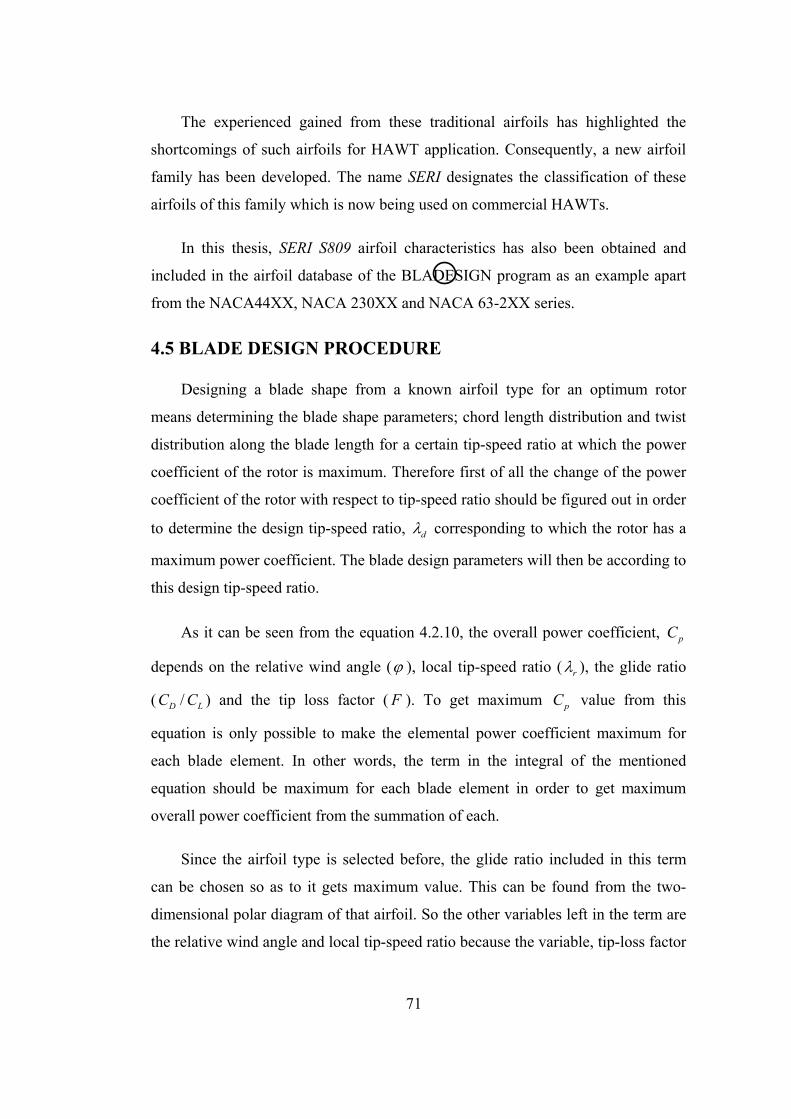
71

The experienced gained from these traditional airfoils has highlighted the

shortcomings of such airfoils for HAWT application. Consequently, a new airfoil

family has been developed. The name SERI designates the classification of these

airfoils of this family which is now being used on commercial HAWTs.

In this thesis, SERI S809 airfoil characteristics has also been obtained and

included in the airfoil database of the BLADESIGN program as an example apart

from the NACA44XX, NACA 230XX and NACA 63-2XX series.

4.5 BLADE DESIGN PROCEDURE

Designing a blade shape from a known airfoil type for an optimum rotor

means determining the blade shape parameters; chord length distribution and twist

distribution along the blade length for a certain tip-speed ratio at which the power

coefficient of the rotor is maximum. Therefore first of all the change of the power

coefficient of the rotor with respect to tip-speed ratio should be figured out in order

to determine the design tip-speed ratio, dλ corresponding to which the rotor has a

maximum power coefficient. The blade design parameters will then be according to

this design tip-speed ratio.

As it can be seen from the equation 4.2.10, the overall power coefficient, pC

depends on the relative wind angle (ϕ ), local tip-speed ratio ( rλ ), the glide ratio

( /D LC C ) and the tip loss factor ( F ). To get maximum pC value from this

equation is only possible to make the elemental power coefficient maximum for

each blade element. In other words, the term in the integral of the mentioned

equation should be maximum for each blade element in order to get maximum

overall power coefficient from the summation of each.

Since the airfoil type is selected before, the glide ratio included in this term

can be chosen so as to it gets maximum value. This can be found from the two-

dimensional polar diagram of that airfoil. So the other variables left in the term are

the relative wind angle and local tip-speed ratio because the variable, tip-loss factor

72

depends also on these two variables for an assumed blade number as it can be seen

from the equation 4.2.1.

Hence a relationship can be established between the relative wind angle and

local tip-speed ratio to determine the optimum relative wind angle, optϕ for a

certain local tip-speed ratio. The condition is given below;

( )( )( )

2sin cos sin sin cos ...

1 cot r r

optD L

FMAX

C C

ϕ ϕ λ ϕ ϕ λ ϕϕ

ϕ

− + → −

A computer program on MATLAB was written to determine the maximum

power coefficient for each blade element (elemental power coefficient) for any set

of values of local tip-speed ratio. The result is given graphically in Figure 4.2 for

an airfoil having glide ratio 0.036

Figure 4.2 Variation of elemental power coefficient with relative wind angles for

different values of local tip-speed ratio.

73

These set of results in Figure 4.2 gives a unique relationship between relative

wind angle and local tip-speed ratio when the maximum elemental power

coefficient is considered. When the optimum relative wind angle values are plotted

with respect to the corresponding local tip-speed ratio values at which the

elemental power coefficient is maximum for a wide range of glide ratios, the

relationship as shown in Figure 4.3 can be found to be nearly independent of glide

ratio and tip-loss factor.

Figure 4.3 Variation of optimum relative wind angle with respect to local tip-speed

ratio at optimum elemental power coefficient for 3B =

Hence the condition given before can be rearranged as following;

( )( ) 2sin cos sin sin cosopt r rMAXϕ ϕ ϕ λ ϕ ϕ λ ϕ≈ − +

74

Therefore a general relationship can be found between optimum relative wind

angle and local tip-speed ratio which will be applicable for any airfoil type by

taking the partial derivative of the term above, i.e.;

( )( ) 2sin cos sin sin cos 0 (4.5.1)r rϕ ϕ λ ϕ ϕ λ ϕϕ∂

− + =∂

Equation 4.5.1 reveals after some algebra [2];

( ) ( )12 3 tan 1 (4.5.2)opt rϕ λ−=

In Figure 4.4 the plot of equation 4.5.2 is shown together with the others

shown in Figure 4.3. As it can be seen from Figure 4.4 below, the relationship

between and opt rϕ λ specified by the equation 4.5.2 can be readily used instead of

establishing different relationships for each airfoil type.

Figure 4.4 Comparison of equation 4.5.2 with the data found for different glide ratios

75

Having found the solution of determining the optimum relative wind angle for

a certain local tip-speed ratio, the rest is nothing but to apply the equations from

equation 4.2.7 to 4.2.10, which were derived from the blade-element momentum

theory and modified including the tip loss factor, to define the blade shape and to

find out the maximum power coefficient for a selected airfoil type.

The procedure of blade design begins with dividing the blade length into N

elements. The local tip-speed ratio for each blade element can then be calculated

with the use of equation 2.5.2 and 3.2.17 as given below;

( ), (4.5.3)r i ir Rλ λ=

Then according to equation 4.5.2 the optimum relative wind angle for each blade

element is determined;

( ) ( )1, ,2 3 tan 1 (4.5.4)opt i r iϕ λ−=

From the equation 4.2.1 the tip loss factor for each blade element is found;

( ) ( ) ( )( )

1

,

/ 2 12 cos exp (4.5.5)

sini

ii opt i

B r RF

r Rπ

ϕ− − − =

The chord-length distribution can then be calculated for each blade element by

using equation 4.2.7;

, , , ,

, , , ,

8 sin (cos sin ) (4.5.6)

(sin cos )i i opt i opt i r i opt i

iL design opt i r i opt i

r Fc

BCπ ϕ ϕ λ ϕ

ϕ λ ϕ−

=+

where ,L designC is chosen such that the glide ratio is minimum at each blade element.

76

The twist distribution can be determined from the following equation which

can be easily derived from the velocity diagram shown in Figure 3.8;

, (4.5.7)i opt i designθ ϕ α= −

Where designα is again the design angle of attack at which ,L designC is obtained.

Finally, the power coefficient is determined using a sum approximating the

integral in equation 4.2.10;

( )

( ) ( )

2, , , ,2

1 2, , , , ,

8 sin cos sin ...

sin cos 1 cot

rN i opt i opt i r i opt i

pi

opt i r i opt i D L opt i r i

FC

C C

λ ϕ ϕ λ ϕλ

ϕ λ ϕ ϕ λ=

∆ − = + −

∑

(4.5.8)

As a result, for a selected airfoil type and for a specified tip-speed ratio and

blade length (i.e. rotor radius), the blade shape can be designed for optimum rotor

and from the calculation of power coefficient the maximum power that can be

extracted from the wind can then be found for any average wind velocity.

As an example, the blade chord-length and twist distribution for an optimum

three-bladed rotor at the design tip-speed ratio 10dλ = is tabulated in Table 4.1 for

the airfoil NACA 4412 whose lift coefficient and drag coefficient values are taken

at 6Re 1 10x= .

77

In Figure 4.5 chord-length distribution with respect to radial location of each

blade element both of which are normalized with blade radius is shown.

Figure 4.5 Chord-length distribution for the designed blade

Similarly twist distribution with respect to radial location is illustrated in

Figure 4.6.

Finally the power coefficient variation with respect to tip-speed ratio is given

graphically in Figure 4.7. From this figure it can be seen that the design tip-speed

ratio should be taken to as 10 where the power coefficient is at maximum value

for the designed blade design.

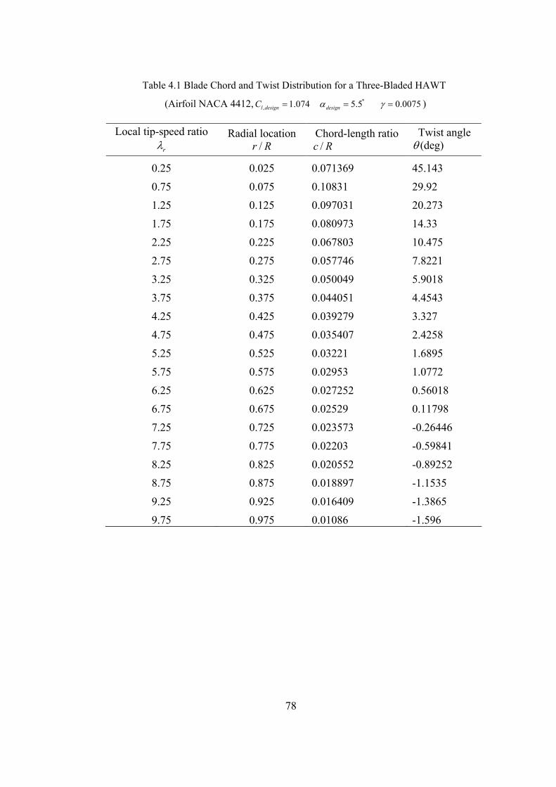
78

Table 4.1 Blade Chord and Twist Distribution for a Three-Bladed HAWT

(Airfoil NACA 4412, , 1.074 5.5 0.0075l design designC α γ= = =° )

Local tip-speed ratio rλ

Radial location /r R

Chord-length ratio /c R

Twist angle (deg)θ

0.25

0.75 1.25

1.75

2.25

2.75

3.25

3.75

4.25

4.75

5.25

5.75

6.25

6.75

7.25

7.75

8.25

8.75

9.25

9.75

0.025

0.075 0.125

0.175

0.225

0.275

0.325

0.375

0.425

0.475

0.525

0.575

0.625

0.675

0.725

0.775

0.825

0.875

0.925

0.975

0.071369

0.10831 0.097031

0.080973

0.067803

0.057746

0.050049

0.044051

0.039279

0.035407

0.03221

0.02953

0.027252

0.02529

0.023573

0.02203

0.020552

0.018897

0.016409

0.01086

45.143

29.92 20.273

14.33

10.475

7.8221

5.9018

4.4543

3.327

2.4258

1.6895

1.0772

0.56018

0.11798

-0.26446

-0.59841

-0.89252

-1.1535

-1.3865

-1.596

79

Figure 4.6 Twist distributions for the designed blade

Figure 4.7 Variation of power coefficient with tip-speed ratio

80

4.6 MODIFICATION OF BLADE GEOMETRY

In general a rotor is not of the optimum shape because of highly loaded of the

designed blade which can be produced from this optimum shape. Furthermore,

when a designed blade is run at a different tip-speed ratio other than the one for

which it is designed, it is no longer optimum. Thus, blade shape is generally

redesigned for he purpose of decreasing the thrust force and torque acting on the

blade during its operation by trying to keep the design power coefficient close to

the one which is obtained for the designed blade.

In the previous section the method of obtaining optimum blade shape has

been introduced and the variation of designed blade geometry parameters (chord-

length and twist) for the airfoil NACA 4412 has been illustrated with figures as an

example. In this section by using the designed blade geometry as a guide,

modification of blade geometry that promises to be a good approximation will be

explained and to illustrate, the modified blade shape will be compared with the

designed one for the airfoil NACA 4412.

4.6.1 MODIFICATION OF CHORD-LENGTH DISTRIBUTION:

The chord-length variation of a designed blade shape is not linear and near the root

the blade chord-length is increasing steeply as it is shown in Figure 4.5. Here such

type of designed blade shape will be modified such that its shape becomes linear

tapered. While transforming the designed blade shape to a linear taper shape, the

area of the designed blade shape is used as necessary information, in other words

the chord-length of each blade element for the both shape should remain the same.

At least the one of linear taper shapes whose blade elements’ chord-lengths are the

closest to the designed blade elements’ chord-lengths should be selected. Also it

should be kept in mind that most power is generated by the outer part of the blade

(between / 0.5 and / 0.9r R r R= = ) [24]. For this reason a blade linearized through

these points of the ideal blade shape seems to be a good choice.

81

Generally, an iterative approach is used. That is, a blade shape can be assumed

and predicted its performance and another blade shape is assumed and the

prediction of performance is repeated until a suitable blade shape has been chosen.

In Figure 4.8 the trapezoidal transformation of the designed blade shape for the

NACA 4412 is shown.

Figure 4.8 Modified blade chord-length variations along the non-dimensional blade radius

4.6.2 MODIFICATION OF TWIST DISTRIBUTION: When the twist

distribution of a designed blade shape is analyzed from the Figure 4.6, it can be

seen that a designed blade has to be twisted strongly, especially near the root again

as it occurs in the chord-length variation of the same blade. For that reason twist

distribution can also be modified considering the ease of fabrication. In this thesis,

this modification has been performed such that twist distribution of the designed

blade has been linearized by using the least-square method [25]. Also at some

distance from blade root the twist becomes negative which generally causes the

blade elements from this distance to blade tip to be stalled. To prevent these blade

82

elements from being in stall region, their twist values are set to zero as shown in

Figure 4.9.

Figure 4.9 Modified twist distribution along the non-dimensional blade radius

4.7 POWER PREDICTION OF MODIFIED BLADE SHAPE

Now that the known parameters are chord-length and twist distribution along

the blade length, the analysis is just reverse of the one which was done for

designing optimum blade shape in section 4.5. In the previous case design angle of

attack, design lift coefficient and glide ratio corresponding to design lift coefficient

were chosen and by so the parameters of blade geometry was found for an

optimum rotor. In this case lift coefficient and angle of attack have to be

determined from the known blade geometry parameters. This requires an iterative

solution in which for each blade element the axial and angular induction factors are

firstly taken as the values which were found for the corresponding designed blade

elements and then determined within an acceptable tolerance of the previous

guesses of induction factors during iteration. The computer program written for this

iteration procedure calculates the induction factors according to the flow chart

given in Figure 4.10.

83

Figure 4.10 Flow chart of the iteration procedure for determining power coefficient of modified blade

Take initial values of , , and F a aϕ ′ from the

designed blade element Eqns: 4.5.4, 4.5.5, 4.2.8, 4.2.9

respectively

Determine angle of attack, αEqn: 4.5.7

Find and L DC C for the determined α using 2-D data of vs and vs L DC Cα α for

the selected airfoil

Calculate local thrust coefficient,

rTC

Eqn: 4.3.3

Update a′ Eqn: 4.2.9

Update a Eqn: 4.2.8

Update a Eqn: 4.3.1

Calculate the differences between updated ,a a′ and

previous guesses

Take updated and a a′ as actual values for

considered blade element

Continue iteration by replacing initial values

with updated ones

When 0.96rTC > When 0.96

rTC <

If differences < 0.01 If differences > 0.01

84

4.8 RESULTS

In this chapter, design of a HAWT blade has been explained and shown the

solution method via the equations derived from BEM theory. Tip-loss factor and

drag effect have also been considered in these equations. The method of

determining blade shape for optimum performance of a turbine has been

developed, how an optimum blade shape is modified for the best performance has

been introduced and finally power performance calculation methods for both have

been established. And the airfoil NACA 4412 was used while performing these

methods and illustrated with figures as an example.

In addition to these studies, the effect of some parameters relating to the blade

design have also been investigated for the purpose of keeping in mind what should

be considered while designing a blade shape for the best performance and the

results are given with figures following this section.

Figure 4.11 shows the maximum achievable power coefficients for a HAWT

with 1, 2 and 3 blades and no drag. The performance for ideal conditions (infinite

number of blades) is also shown. It can be seen that the fewer the blades the lower

the possible PC at the same tip-speed ratio. For that reason most wind turbines use

two or three blades and in general most two-bladed wind turbines use a higher tip-

speed ratio than most three-bladed wind turbines. Thus, there is little practical

difference in the maximum achievable PC value between typical two- and three-

bladed designs, assuming no drag. Moreover, the effect of the number of blades is

negligible at high design tip-speed ratios.

The effect of glide ratio on maximum achievable power coefficients for a

three-bladed rotor is shown in Figure 4.12. There is clearly a significant reduction

in maximum achievable power as the airfoil drag increases. It can be seen that it

clearly benefits the blade designer to use or design airfoils with low glide ratio.

85

The radial variation in relative wind angle ϕ for different design conditions

is shown in Figure 4.13. The angle ϕ is high at all radial sections for the low

design tip-speed ratio. The increase in drag marginally reduces the angleϕ . The

reduction in the number of blades reduces the relative wind angle at the low design

tip-speed ratio, but the effect of number of blades is negligible at the high values of

design tip-speed ratio.

In this study the modification of the designed blade shape has also been

determined. The modification of chord-length keeping the twist distribution same

with that of designed blade, the modification of twist distribution keeping the

chord-length distribution same with that of designed blade and modification of both

have been separately determined and their performance have been compared.

The variations in twist angle and chord-length along the blade for different tip-

speed ratios are shown in Figure 4.14 and Figure 4.15. In Figure 4.16 and

Figure 4.17, the variations in twist angle and chord-length for different tip-speed

ratios are given after modifying the chord-length distribution of the designed blade.

Figure 4.18 shows the variations in modified twist along the blade length for

different tip-speed ratios and the variation of angle of attack along the blade length

for this blade whose twist distribution has been modified is shown in Figure 4.19

together with the design angle of attack and stall angle for considered airfoil.

Figure 4.20 shows the variation in angle of attack along the blade length for a

designed blade whose both chord-length and twist distributions have been

modified.

In Figure 4.21 power coefficients of modified blades are compared with that of

designed blade. It can be seen from these figures that the design power coefficient

of modified blade, which is attained after modification of the designed blade

performed in this thesis, is fairly close to the design power coefficient of the

designed bade at different design tip-peed ratio. Moreover, since the power

86

coefficient is directly proportional to the lift forces acting on the blade,

modification of the designed blade causes the lift forces acting on the modified

blade to decrease with regard to the lift forces acting on the designed blade

preventing the blade from loading highly during its operation.

Radial thrust coefficient which is a measure of loading of rotor in the wind

direction has also been calculated for the designed and the modified blade and

shown in Figure 4.22 and Figure 4.23. Again thrust force is also decreased for the

modified blade as to the thrust force for the designed blade.

Off-design conditions of turbines have been taken into consideration and

regarding the cut-in and cut-out speed, the working range of a fixed-rotational

speed turbine has been determined separately for the designed blade and the

modified blade. As shown in Figure 4.24 and Figure 4.25 the working range of

modified blade is drastically reduced with regard to that of designed blade.

The performance of a HAWT rotor during its operation at different average

wind velocities is also studied. In this study three-bladed HAWT rotor is designed

for the required power production 50 kW and at the design wind velocity 8 m/s.

For these conditions the rotational velocity of the rotor becomes 76 rpm in case of

using designed blade and 59 rpm for the modified blade. And for different average

wind velocities, corresponding power production of this three-bladed HAWT is

obtained as shown on Table 4.2. Since the power production is proportional with

the cube of the average wind velocity (equation 2.5.1) and the power coefficient of

the designed blade is nearly constant over a wide range of tip-speed ratio as

illustrated in Figure 4.21, power production of HAWT rotor made up from the

designed blades is gradually increasing as the average wind velocity increases.

Power production of a HAWT rotor made up from the modified blades, however, is

not increasing very much as expected when its power coefficient variation with

respect to tip-speed ratio shown on Figure 4.21 is analyzed.

87

The effect of Reynolds number on power performance of wind turbines has

been studied. Since two-dimensional airfoil characteristics depends on the

Reynolds number, there should be effect on the power of turbines but as shown in

Figure 4.26 it is not significant as expected.

In Figure 4.27 and Figure 4.28, the views of blade elements of NACA 4412

airfoil for the designed and its modified blade are shown. As it can be seen from

these figures, twist distribution of modified blade becomes smoother than that of

designed blade.

Figure 4.29 and Figure 4.30 show the blade elements of NACA 4412 in

isometric view for the designed and modified blade. Note that the modification of

the designed blade makes chord-length of some blade elements near the root bigger

than that of designed blade but the variation of chord-length from root towards tip

becomes linear for the modified blade as to the sharp variation for the designed

blade.

Lastly, three-dimensional views of the designed and modified blade made

from the airfoil NACA 4412 are illustrated in Figure 4.31 and Figure 4.32 for

visualization.

88

Figure 4.11 Effect of number of blades on peak performance of optimum wind turbines

Figure 4.12 Effect of Drag/Lift ratios on peak performance of an optimum three-bladed

wind turbine

89

Figure 4.13 Effect of drag and tip losses on relative wind angle for optimum design

Figure 4.14 Relative wind angles for optimum performance of three-bladed wind

turbines

90

Figure 4.15 Blade chord-length distributions for optimum performance of three-bladed

wind turbines

Figure 4.16 Twist angle distributions for modified chord-length of the designed blade

91

Figure 4.17 Chord-length distribution of a modified blade for different tip-speed ratio

Figure 4.18 Twist distributions for modified blade of the designed blade

92

Figure 4.19 Distribution of angle of attack for modified twist of the designed blade

Figure 4.20 Distribution of angle of attack for modified twist and chord-length of the

designed blade

93

Figure 4.21 Comparison of power coefficients of modified blades with the designed blade

Figure 4.22 Radial thrust coefficient variation of the designed blade

94

Figure 4.23 Radial thrust coefficient for modified twist and chord-length of the designed

blade

Figure 4.24 Working range of the designed blade designed at 10λ =

95

Figure 4.25 Working range of modified twist and chord-length of the designed blade

designed at 10λ =

Figure 4.26 Effect of Reynolds number on peak performance of an optimum three-bladed

turbine

96

Figure 4.27 Views of blade elements from root towards tip for the designed blade

Figure 4.28 Views of blade elements from root towards tip for the modified blade

97

Figure 4.29 Isometric views of the blade elements for the designed blade

Figure 4.30 Isometric views of the blade elements for the modified blade

98

Figure 4.31 Three-dimensional solid model of the designed blade

99

Figure 4.32 Three-dimensional solid model of the modified blade

100

Table 4.2 Power Production of a fixed rotational three-bladed HAWT (Airfoil: NACA-4412, Designed at P=50 kW, U∞=8 m/s)

Power Production (kW)

U∞(m/s) Designed Blade (Ω=76 rpm)

Modified Blade (Ω=59 rpm)

6 21 10

8 50 50

10 97 78

12 166 105

14 260 136

16 381 163

18 532 195

101

CHAPTER 5

COMPUTER PROGRAM FOR BLADE DESIGN

1.2 INTRODUCTION

The computer programs XFOILP4 and MATLAB are utilized during the

study of this thesis. This chapter focuses on these programs, results from the

programs and their applications in computer-aided design of horizontal-axis wind

turbine blades.

XFOIL is firstly introduced by giving its capabilities on the analysis of an

existing airfoil, design and redesign of new airfoil geometric parameters. Since the

aerodynamic characteristics of an airfoil should be known numerically before

designing a blade and all the information and experimental results performed on

airfoils were given graphically in literature, XFOIL is very well fitted for

obtaining lift coefficient and drag coefficient data with respect to angle of attack.

In this thesis only the function of this program related to the viscous analysis of

existing airfoils has been used. The required data are obtained from the program by

performing on various existing airfoil types and used for the subsequent studies of

blade design. The procedure to obtain the data is described and the results of the

program are also compared with the results given in literature to show that the

program XFOIL gives fairly close values.

User-interface computer program, BLADESIGN written by using MATLAB

is then described. General view and working flow chart of the program are

presented with the explanation of important properties and capabilities of the

program. All the commands and their functions in the program are also introduced

for the users of this program.

Lastly sample blade design studies are given by specifying a set of input

values. According to these input values, the program is executed and the

102

corresponding outputs are illustrated in tabulated form and also compared with

CP & λ, c/R & r/R and θ & r/R figures for both designed and modified blades.

1.2 XFOILP4

XFOIL is an interactive program for the design and analysis of subsonic

isolated airfoils. It consists of a collection of menu-driven routines which perform

various useful functions such as:

− Viscous (or incviscid) analysis of an existing airfoil, allowing

• Forced or free transition

• Transitional separation bubbles

• Limited trailing edge separation

• Lift and drag predictions just beyond maximum lift coefficient

• Karman-Tsien compressibility correction

− Airfoil design and redesign by interactive specification of a surface speed

distribution via screen cursor or mouse. Two such facilities are implemented:

• Full-Inverse, based on a complex-mapping formulation

• Mixed-Inverse, allowing relatively

− Airfoil redesign by interactive specification of new geometric parameters such

as:

• New max. thickness and/or camber

• New LE (leading edge) radius

• New TE (trailing edge) thickness

103

• New camberline via geometry specification

• New camberline via loading change specification

• Explicit contour geometry (via screen cursor)

− Drag polar calculation with fixed or varying Reynolds and/or Mach number

− Writing and reading of airfoil geometry and polar save files

− Plotting of geometry, pressure distribution and polars

XFOIL was written by Mark Drela in 1986 with the name XFOIL 1.0 and after

undergoing numerous revisions, upgrades and enhancements it becomes now

strongly geared to practical airfoil development with its final revision name

XFOILP4. Further explanation about the use of XFOIL program can be found in

reference [26], here only the part of XFOIL program which was extensively used

for the development of blade design program will be described.

If it is remembered from the airfoil selection criteria in section 4.4, the design

angle of attack should be selected such that the glide ratio is minimum at that value

of angle of attack. Therefore the variation of lift coefficients and drag coefficients

of an airfoil with respect to angle of attack in the fully-attached regime are

required. XFOIL gives these data in a considerably excellent agreement with

published polars as shown in Figure 5.1 and Figure 5.2 for the airfoil NACA 4412

as an example. The results of XFOIL has been compared with the reference polar

data performed by Abbott and Von Doenhoff [27] and also from the reference

Riegels [28] to see the validity of XFOIL results.

104

Figure 5.1 Comparison of XFOIL lift coefficient data with data in reference [28]

Figure 5.2 Comparison of XFOIL drag coefficient data with data in reference [28]

The results are obtained from the program by giving the coordinates of an

airfoil. XFOIL first takes these coordinates and creates the contour geometry of the

airfoil and finally by dividing the surface of the airfoil into a certain number of

105

panels, which can be changed by the user, gives the variations of lift coefficient

and drag coefficient with respect to angle of attack.

In developing the airfoil database for the blade design program, the

characteristics of airfoil have been obtained with the viscous mode analysis of

XFOIL and for the Reynolds number in the order of 1 million and also Mach

number has been setted to zero considering that the angular velocity of a HAWT

blades does not become so great that the rotational velocity of the blade tips

approaches to the velocity of sound.

5.2 BLADESIGN

As it was stated before, the main objective of this thesis is to develop a user-

interface computer program on HAWT blade design. The main purpose of

constructing such a program is to collect and represent all the studies of this thesis

in a visual and more understandable way and also to provide a design program for

the users who are dealing with HAWT blade design. For all of these reasons a user-

interface computer program on HAWT blade design was written.

The general view of the program and its working flow schematic are illustrated

in Figure 5.3 and Figure 5.4 respectively. The main features of the program can be

summarized as below:

• The program was written on MATLAB, version 6 [29].

• The program gives various error dialog boxes in case of incorrect input data

or requesting an output of a command before this command some other commands

should be executed firstly and necessary outputs for the requesting command

should be firstly obtained. By so the program serves as a guide for the user to

perform the design procedure step by step.

• The density of air, ρ is taken as 1.2 kg/m3 in some algorithms of the

program for the calculation of rotor diameter.

106

• The program includes one input part and four output parts.

• Input part requires the following information; turbine power required in

Watt, design wind velocity in m/s, the number of blades supposed to be used on the

rotor and airfoil type to be used for the blade profile. Here the design wind velocity

is the average wind velocity of an area where the turbine or windfarm of similar

turbines is to be set. Following airfoils are currently available in the database;

NACA 4412, NACA 4415, NACA 4421, NACA 23012, NACA 23015, NACA

23021, NACA 63-210, NACA 63-212, NACA 63-218, NACA 63-221 and SERI-

S809.

• The output parts are composed of design condition output, blade geometry

output, 3-D visualization output and figures output.

Design condition output part gives the information for both designed blade

and its modified blade. These information are design power coefficient (CP),

corresponding design tip-speed ratio (λd) and rotor diameter in meter to be

constructed for the specified turbine power input.

Blade geometry output part shows the chord-length in meter and setting

angle in degree for each blade element (for each station) and does this again for

both designed and modified blade. The number of stations in the program has been

kept constant with 30 because it has been seen that the increase of number of

stations does not change the blade geometry values considerably much. The

purpose of putting this output part is that these output information can be used for

the prototype production of the design blade in further studies.

3-D visualization output part gives three dimensional views of the designed

and modified blades on separate windows.

The last output part, figures output part illustrates the results with figures for

both designed and modified blade. The first figure shows the variation of power

coefficient with tip-speed ratio, the second one shows the distribution of setting

angle in degrees with respect to normalized blade length (r/R) and the last figure is

107

for the output of chord-length distribution, which is normalized with R, with

respect to again normalized blade length (r/R) graphically. These figures can be

analyzed visually to compare the performance and blade geometry of designed and

modified blade by making both of the outputs visible.

• If it is desired to change the input values for another design, the command

‘change inputs’ in the input part stands for this purpose. By pressing this button,

all the outputs will become vanished and the program gets ready for the new input

values.

• Blade geometry output (chord-length and setting angle values for each

station) can be saved to a file in the working directory with the command ‘save

blade geometries’ or can be print out with the command ‘print’ and the program

closes with the command ‘exit’’ under the file menu option.

108

Figure 5.3 General view of BLADESIGN

109

Figure 5.4 Flow Schematic of HAWT Blade Design program

5.3 SAMPLE BLADE DESIGN ON BLADESIGN PROGRAM

In this section a sample blade design will be demonstrated on blade design

program according to the following inputs:

Turbine power required, P = 50 kW (50000W)

Design wind velocity, U∞ = 13 m/s

Number of blades, B = 3

Airfoil type = SERI-S809

First task is to find the design power coefficient which is dependent on the

selected airfoil type. Then the design tip-speed ratio at which the maximum power

coefficient (i.e. design power coefficient) can be obtained for the three-bladed

rotor. This design tip-speed ratio can be used to determine the rotational velocity of

the rotor at design condition. Finally rotor diameter is found out with the known

values of design power coefficient and design wind velocity and required power.

(Equation 2.5.1)

I N P U T S

E X E C U T I O N

O U T P U T S

Turbine Power Required, P (W)

Design Wind Velocity, U∞ (m/s)

Number of Blades, B

Airfoil Type

Design Conditions

Designed Blade

Modified Blade

Blade Geometry

Designed Blade

Modified Blade

Stations (Blade elements)

Stations (Blade elements)

Figures

Designed Blade Modified Blade

CP & λ c/R & r/R θ & r/R c/R & r/R θ & r/R CP & λ

3-D visualization

3-D view of modified blade

Design Power Coefficient,CP

Design Tip-Speed Ratio

Rotor Diameter, D (m)

Design Power Coefficient,CP

Design Tip-Speed Ratio

Rotor Diameter, D (m)

Chord-Length Distribution (m)

Setting Angle Distribution (deg)

Chord-Length Distribution (m)

Setting Angle Distribution (deg)

3-D view of designed blade

110

Design conditions output part calculates the mentioned values for both

designed and modified blade. Pressing the ‘designed’ and ‘modified’ pushbuttons

in the design coefficient output part, those values shown in Table 5.1 will be

obtained from the program. Note that design tip-speed ratio is same for both blades

because the designed blade is modified at its design tip-speed ratio. Also note that

when the designed blade is modified, the power is decreased by 10% of the

designed one or for the same power output the rotor diameter should be increased

by about 7% of the designed rotor diameter.

Table 5.1 Design conditions output for designed and modified blade (P= 50 kW, U∞= 13 m/s, B=3, SERI-S809 airfoil)

Output Designed Blade Modified Blade

Design Power Coefficient 0.495 0.44

Design Tip-Speed Ratio 8.5 7

Rotor Diameter (m) 9.8 10.5

The second output part documents the chord-length and setting angle

distributions for each blade element beginning from approximately 1.5% of the

blade length and ending at 98% of the blade length. In other words program

calculates the blade geometry parameters dividing the total blade length into 30

elements. Pressing again the ‘designed blade’ and ‘modified blade’ pushbuttons in

the blade geometry output part, those values shown in Table 5.2 will be obtained

from the program.

111

Table 5.2 Blade Geometry output for designed and modified blade

(P= 50 kW, U∞= 13 m/s, B= 3, SERI-S809 airfoil)

Designed Blade Modified Blade Stations

(Blade elements) Chord-

Length c (m)

Setting angle θ (deg)Chord-

Length c (m)

Setting angle θ (deg)

1 2 3 4 5 6 7 8 9 10 11 12 13 14 15 16 17 18 19 20 21 22 23 24 25 26 27 28 29 30

0.367 0.754 0.852 0.825 0.758 0.685 0.617 0.558 0.507 0.463 0.426 0.394 0.365 0.341 0.320 0.300 0.283 0.268 0.254 0.241 0.230 0.220 0.201 0.200 0.190 0.180 0.167 0.151 0.125 0.078

49.1 39.1 30.9 24.6 19.9 16.3 13.5 11.3 9.5 8.1 6.8 5.8 5.0 4.2 3.6 3.0 2.5 2.1 1.7 1.4 1.0 0.7 0.4 0.2

-0.03 -0.25 -0.4 -0.6 -0.8 -1

0.780 0.756 0.732 0.710 0.686 0.662 0.640 0.616 0.592 0.570 0.546 0.522 0.499 0.475 0.452 0.430 0.405 0.382 0.360 0.335 0.312 0.289 0.265 0.242 0.219 0.195 0.172 0.149 0.125 0.102

25.7 24.6 23.3 22.2 21.0 19.8 18.6 17.5 16.3 15.1 13.9 12.7 11.5 10.3 9.2 8.0 6.8 5.6 4.5 3.3 2.1 0.9 0 0 0 0 0 0 0 0

For the comparison of power coefficient and blade geometry parameters

(chord-length and twist distribution) between designed blade and its modified one

their figures can be plotted on the right half of the program. If ‘designed’ toggle

112

button in blue color is pressed, figures related to designed blade will be plotted

with blue color and when the toggle button becomes in depressed position by

pressing it again, figures related to the designed blade will be erased. Similarly if

‘modified’ toggle button in red color is pressed, figures related to modified blade

will be plotted with red color and will be erased in case of depressed position of the

toggle button. Power coefficient with respect to tip-speed ratio, setting angle

variation with respect to normalized blade length (r/R) and normalized chord-

length distribution (c/R) with respect to normalized blade length (r/R) figures for

the sample blade design case are shown in Figure 5.5, Figure 5.6 and Figure 5.7

respectively.

Note that as discussed in chapter 4 the working range of modified blade

becomes very narrow with respect to that of designed blade for a fixed rotational

speed rotor.

Figure 5.8 and Figure 5.9 shows the three dimensional views of designed and

modified blade for the sample blade design case as one activates the push buttons

under the 3-D visualization output part.

Finally how the results which have been given in tabulated form here looks on

the user-interface program for this sample blade design case are given in

Figure 5.10.

Figure 5.5 Comparison of power coefficient of designed and modified blade

(P= 50 kW, U∞= 13 m/s, B=3, SERI-S809 airfoil)

113

Figure 5.6 Comparison of setting angle variation of designed and modified blade

(P= 50 kW, U∞= 13 m/s, B=3, SERI-S809 airfoil)

Figure 5.7 Comparison of chord-length distribution of designed and modified blade

(P= 50 kW, U∞= 13 m/s, B=3, SERI-S809 airfoil)

114

Figure 5.8 Three-dimensional view of the designed blade (P= 50 kW, U∞= 13 m/s, B=3, SERI-S809 airfoil)

Figure 5.9 Three-dimensional view of the modified blade (P= 50 kW, U∞= 13 m/s, B=3, SERI-S809 airfoil)

115

Figure 5.10 Output from the program performed for the sample blade design case

(P= 50 kW, U∞= 13 m/s, B=3, SERI-S809 airfoil)

116

5.4 COMPARISON OF OUTPUTS

The program was executed for each airfoil in the database and the outputs of

design conditions were obtained as illustrated in Table 5.3. The design angle of

attack and corresponding glide ratios (CD/CL) for each airfoil are also put in this

table in order to see the effect of glide ratio on the design power coefficient.

When the design power coefficients of the airfoils are compared, it is seen that

the glide ratio decreases the design power coefficient as it was stated before. And

the reduction in design power coefficient of the designed blade becomes

approximately 10% after modification of the designed blade. Similarly for the same

power output, the increase in the rotor diameter of the designed blade becomes

about 5% after modification.

Table 5.3 Comparison of outputs for the airfoils

(P= 50kW, U∞=10 m/s, B=3)

117

In Table 5.4 the rotor diameters for different turbine power outputs for both

designed and modified blade are given. It is seen that the modification of the design

blade increases the rotor diameter but this increase may be accepted regarding the

moderate loading of the modified blades as it was explained in chapter 5.

Table 5.4 Comparison of rotor diameters for different turbine power outputs

(U∞=13m/s, B=3, SERI-S809)

118

CHAPTER 6

CONCLUSION

In this study, aerodynamic design of horizontal-axis wind turbine blades was

investigated and a user-interface computer program called as BLADESIGN was

written on HAWT blade design software for the use of its outputs in further studies.

Wind turbine blades are the pivot of the other parts of a wind turbine in

electricity production since they extract the energy from the wind and carry this

energy to generators which produce electricity. The interaction between the wind

and the blades is related to the aerodynamic forces acting on the blades. While the

wind is passing through the area swept by a rotor it leaves its some part of energy

on the blades resulting from this aerodynamic interaction. Hence it is limited to the

aerodynamic aspect during the study of HAWT blade design.

Aerodynamic theories related to HAWT blade design were investigated

extensively. Firstly the simplest aerodynamic model of a HAWT, the actuator disk

theory was discussed. The main outcome of this theory is that it is impossible to

extract more than 59% of the usable amount of wind energy under the ideal

conditions which were stated as the assumptions of this theory.

Since the actuator disk theory is an idealized model which will never be

realized for real operation of wind turbines, the general momentum theory is then

needed to be discussed. The main outcome of this theory is a measure of the effects

of rotation on the relative values of the induced velocities at the rotor and in the

wake.

Although the general momentum theory predicts the rotor performance, it fails

to give any information about the rotor geometry. This deficiency requires the next

discussion which is blade element theory. In the blade element theory, the

119

equations required to find the torque and thrust force on the rotor were found in

terms of blade geometry parameters. The results of this theory provide to make

relations between the rotor performance and rotor geometry.

The ultimate goal was to relate the results of general momentum theory and

blade element theory in order to get the enough equations for HAWT blade design.

This was achieved in the discussion of blade element-momentum theory (BEM).

After the equations resulted from this theory were obtained, a tip correction method

was applied to the theory. In this study, linearized tip correction method was used

to take the effect of number of blades into account. This method uses Prandtl’s tip

correction factor which is related to the reduction of the circulation around a rotor

blade.

It was also briefly explained about vortex theory for the purpose of giving the

physical explanation of induced velocity definitions made in the previous theories.

The origin of axial and angular induction factors was explained and the

assumptions of the previous theories were clarified with the explanation of this

theory.

Blade design was performed beginning with the optimization of blade

geometry aerodynamically. Aerodynamic optimization for a wind turbine means to

design a blade geometry which gives the maximum power output. For the

optimization, it was graphically shown that the effect of airfoil characteristics

(glide ratio) and the tip-loss effect were negligible on rotor performance. So the

unique relationship was found between the relative wind angle and local tip-speed

ratio for the determination of optimum condition for each blade element. For a

chosen blade profile and a tip-speed ratio, the setting angle and chord-length

variation along the blade length were then calculated together with the power

coefficients. The calculations shows that power coefficient increases with

increasing design lift coefficient and decreasing drag coefficient of blade profile.

This means that the development in profile data is needed for better optimization.

120

Designed blade has a non-linear twist and taper and more importantly even

though it had high power coefficient, it was highly loaded. Therefore, in this study,

the blade geometry was simplified and performance of modified blade was

examined. At first, the strongly non-linear taper was replaced with a linear taper.

Among the modified blades whose surfaces are equal to the designed blade’s ones,

the one which has the highest power output was chosen. Then the large blade twist

was replaced with a linear blade setting angle distribution. Under these conditions,

it was seen that the new modified blade reduced power output approximately 10%

of the power output of the designed blade. This means that in order to extract the

same amount of power with the designed blade, the blade span must be expanded

approximately 5%.

Finally, all the studies on HAWT blade design were presented on a user-

interface computer program written on MATLAB. User of the blade design

program gives the required power output, number of blades, blade profile and

design wind velocity as input and the program gives design power coefficient,

design tip-speed ratio and rotor diameter as output for both designed and modified

blade. In addition to that, blade geometries were listed for again both designed and

modified blade. The graphical illustration of figures for the comparison of designed

and modified blade and three dimensional views of both blades were what the

program does lastly.

The studies of this thesis can be surely used for further works. These further

works might be either directly parallel to the topic of this thesis to add valuable

usefulness on horizontal-axis wind turbine blade design or related to the studies of

this thesis to extend the studies on horizontal-axis wind turbines as they are

described in the following paragraphs.

If it is recalled that the modification of a designed blade was carried out for

linear taper of chord-length distribution and linear variation of setting angle

distribution using least square method, other alternative methods for modification

121

may also be tried and their performance may be compared with their designed

blades and with the ones obtained in this study.

In this study, the other constrain is the use of the known airfoil types. Apart

from these, new airfoil designs may be made by the use of XFOIL program and a

method of designing new airfoil shapes which show reasonably high performance

may be proposed.

The lift and drag behaviors of airfoils are measured in wind tunnels under non-

rotating conditions. Investigations have shown that the same airfoils, when used on

a horizontal-axis wind turbine, may exhibit delayed stall and may produce more

power than expected. So the rotor performance prediction considering the delayed

stall of airfoils in the operation of HAWTs may be studied.

Besides, blade element-momentum (BEM) theory approach has been used to

design HAWT blades. There are other approaches to predicting blade performance

and to designing blades that may be more applicable in some situations. Vortex

wake method, for example, might be used and results of this method can be

compared with the results of BLADESIGN.

Structural design of HAWT blades is as important as their aerodynamic

design. The dynamic structural loads which a rotor will experience play the major

role in determining the lifetime of the rotor. Obviously, aerodynamic loads are a

major source of loading and must be well understood before the structural response

can be accurately determined and also the blade geometry parameters are required

for dynamic load analysis of wind turbine rotors. So such a study on the dynamic

load analysis of HAWT blades might also use the outputs of BLADESIGN.

122

REFERENCES

1- Spera, D. A., “Wind Turbine Technology”, Asme Press, 1998

2- Manwell, J. F., McGowan, J. G., Rogers, A. L., “Wind Energy Explained; Theory, Design and Application”, John Wiley & Sons Ltd, 2002

3- Golding, E. W., “The Generation of Electricity by Wind Power”, London E. & F. M. Spon Ltd. A Halsted Press Book, 1976

4- Kovarik, T., Pipher C., Hurst, J., “Wind Energy”, Prism Press, 1979

5- Uyar, T. S., “Türkiye Enerji Sektöründe Karar Verme Ve Rüzgar Enerjisinin Entegrasyonu”, Kocaeli Üniversitesi, Teknik Eğitim Fakültesi, 2000

6- European Wind Energy Association, “ WIND FORCE 10, A Blue Print to Achieve 10% of the World’s Electricity From Wind Power By 2020”, 2000

7- Hansen, A. C., Butterfield, C. P., “Aerodynamics of Horizontal-Axis Wind Turbines”, Annual Review of Fluid Mechanics, Vol.25, 1993

8- Le Gourieres, D., “Wind Power Plants, Theory and Design”, Pergamon Press, 1982

9- Duncan, W. J., “An Elementary Treatise on the Mechanics of Fluids”, Edward Arnold Ltd, 1962

10- Durand, W. F., “Aerodynamic Theory, Volume 2”, Dover Publications, Inc., 1963

123

11- Rijs, R. P. P., Smulders, P. T., “Blade Element Theory for Performance Analysis of Slow Running Wind Turbines”, Wind Engineering, Vol.14 No.2, 1990

12- Lock, C. N. H., “Experiments to Verify the Independence of the Elements of an Airscrew Blade”, Br. A.R.C.R and M.953, 1924

13- Wilson, R. E., Lissaman, P. B. S., Walker, S. N., “Aerodynamic Performance of Wind Turbines”, Energy Research and Development Administration, 1976

14- Glauert, H., “The Elements of Airfoil and Airscrew Theory”, Cambridge Univ. Press, 1983

15- Zhiquan, Y., Zhaoxue, C., Jingyi, C., Shibao, B., “Aerodynamic Optimum Design Procedure and Program for the Rotor of a Horizontal-Axis Wind Turbine”, Journal of Wind Engineering and Industrial Aerodynamics, Vol.39, 1992

16- Afjeh, A. A., Keith, T. G., “A Simple Computational Method for Performance Prediction of Tip-Controlled Horizontal Axis Wind Turbines”, Journal of Wind Engineering and Industrial Aerodynamics, Vol.32, 1989

17- Gould, J., Fiddes, S. P., “Computational Methods for the Performance Prediction of HAWTs”, ”, Journal of Wind Engineering and Industrial Aerodynamics, Vol.39, 1992

18- Pandey, M. M., Pandey, K. P., Ojha, T. P., “An Analytical Approach to Optimum Design and Peak Performance Prediction for Horizontal Axis Wind Turbines”, ”, Journal of Wind Engineering and Industrial Aerodynamics, Vol.32, 1989

19- Nathan, G. K., “A Simplified Design Method and Wind-Tunnel Study of Horizontal-Axis Windmills”, ”, Journal of Wind Engineering and Industrial Aerodynamics, Vol.6, 1980

124

20- Vossinis, A., Voutsinas, S., “Computer-Aided Design of Blades: Current Capabilities and Perspectives”, http://www.fluid.mech.ntua.gr/wind/avis/avigotem.html

21- Munduate, X., Coton, F. N., “An Aerodynamic Method for the Preliminary Design of Horizontal Axis Wind Turbines”, Journal of Advanced Engineering Design, Vol.40, No.1, 2000

22- De Vries, O., “Fluid Aspects of Wind Energy Conversion”, AGARD Report 243, 1979

23- Timmer, W. A., van Rooy, R. P. J. O. M., “Thick Airfoils for HAWTs”, Journal of Wind Engineering and Industrial Aerodynamics, Vol.39, 1992

24- Rijs, R. P. P., Jacobs, P., Smulders, P. T., “Parameter Study of the Performance of Slow Running Rotors”, Journal of Wind Engineering and Industrial Aerodynamics, Vol.39, 1992

25- Kreyszig, E., Norminton, E. J., “Advanced Engineering Mathematics”, John Wiley & Sons Ltd, 8th Edition, 2002

26- Drela, M., “XFOIL Subsonic Airfoil Development System”, http://raphael.mit.edu/xfoil , 2001

27- Abbott, I. H., von Doenhoff, A. E., “Theory of Wing Sections, including a summary of airfoil data”, Dover Publications, 1959

28- Riegels, F. W., “Aerofoil Sections; results from wind-tunnel investigations, theoretical foundations”, Butterworths, 1961

29- MATLAB The Language of Technical Computing, “Building GUIs with MATLAB”, Version 6, The Mathworks, Inc., 2002