index structures in biological sequence analysisstoye/dropbox/20070315... · index structures in...
TRANSCRIPT
Index Structures in Biological Sequence AnalysisFrom Simplicity to Complexity and Back
Jens Stoye
AG Genominformatik, Technische Fakultat
Institute of Bioinformatics, Center of Biotechnology
Bielefeld University, Germany
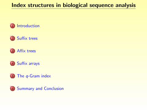
Index structures in biological sequence analysis
1 Introduction
2 Suffix trees
3 Affix trees
4 Suffix arrays
5 The q-Gram index
6 Summary and Conclusion

Index structures in biological sequence analysis
1 Introduction
2 Suffix trees
3 Affix trees
4 Suffix arrays
5 The q-Gram index
6 Summary and Conclusion

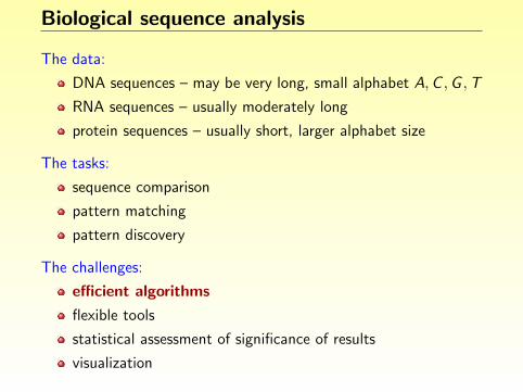
Biological sequence analysis
The data:
DNA sequences – may be very long, small alphabet A,C ,G ,T
RNA sequences – usually moderately long
protein sequences – usually short, larger alphabet size
The tasks:
sequence comparison
pattern matching
pattern discovery
The challenges:
efficient algorithms
flexible tools
statistical assessment of significance of results
visualization

Some applications
Sequence comparison
alignment, multiple alignmentsimilar sequence → similar structure → similar function
Pattern matching
mapping of expressed sequence tags (ESTs) on genomic DNAtargets of a given miRNApalindromic or other RNA structural patternsknown repeats (for further exclusion from analysis)
Pattern discovery
unknown promoter binding sitesrepeats, tandem repeatspossible DNA methylation sites
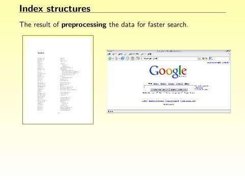
Index structures
The result of preprocessing the data for faster search.
Inde x
abstract, 72boolean, 28byte, 28case, 3 5catch, 9 8char, 28class, 21default, 3 5double, 21 , 28do, 3 1else, 3 2extends, 23 , 6 6false, 26finally, 9 8final, 21float, 28for, 3 1if, 26 , 3 2implements, 9 0import, 23 , 9 4instanceof, 9 9int, 25 , 28length, 26long, 28new, 21package, 23 , 9 3private, 24 , 6 2protected, 24public, 24short, 28static, 21 , 22, 6 1String, 28 , 3 9super, 6 8switch, 3 5this, 6 0throws, 9 7throw, 9 7true, 26
try, 9 8void, 22while, 26 , 3 1
a bstra k teK la ssen, 71Metho den, 71
a bstra k te D a tenty pen, 5 5Alg o rithmen
B o y er-Mo o re (B M), 4 3B o y er-Mo o re-Ho rspo o l (B MH), 4 4K nuth-Mo rris-Pra tt (K MP), 4 6T ex tsucha lg o rithmen, 3 9
Arra y , 26mehrdimensio na l, 3 3
Ausg a be, 1 1 3Ausna hmen, 9 4
B a ck us-Na ur-Fo rm, 8B ito pera to ren, 3 0B NF, 8B o o l’sche O pera to ren, 29B o y er-Mo o re (B M), 4 3B o y er-Mo o re-Ho rspo o l (B MH), 4 4
ca ll by reference, 6 5ca ll by v a lue, 6 4ca sting , 6 7
D a tena bstra k tio n, 5 5D a tenk a pselung , 5 5D a tenstro me, 1 1 7D a tenty p
a bstra k t, 5 5Sta ck , 5 6
D ek rement, 3 0direk te V erk ettung , 1 0 7D o k umentierung , 6 3D o uble Ha shing , 1 0 8
1 23
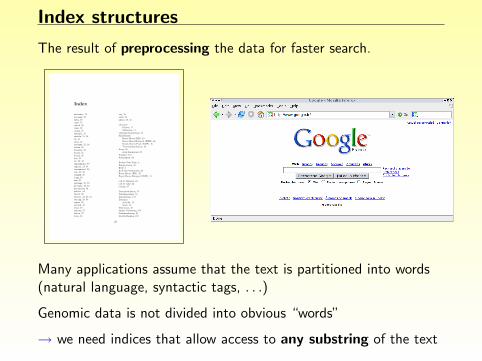
Many applications assume that the text is partitioned into words(natural language, syntactic tags, . . .)
Genomic data is not divided into obvious “words”
→ we need indices that allow access to any substring of the text
Index structures
The result of preprocessing the data for faster search.
Inde x
abstract, 72boolean, 28byte, 28case, 3 5catch, 9 8char, 28class, 21default, 3 5double, 21 , 28do, 3 1else, 3 2extends, 23 , 6 6false, 26finally, 9 8final, 21float, 28for, 3 1if, 26 , 3 2implements, 9 0import, 23 , 9 4instanceof, 9 9int, 25 , 28length, 26long, 28new, 21package, 23 , 9 3private, 24 , 6 2protected, 24public, 24short, 28static, 21 , 22, 6 1String, 28 , 3 9super, 6 8switch, 3 5this, 6 0throws, 9 7throw, 9 7true, 26
try, 9 8void, 22while, 26 , 3 1
a bstra k teK la ssen, 71Metho den, 71
a bstra k te D a tenty pen, 5 5Alg o rithmen
B o y er-Mo o re (B M), 4 3B o y er-Mo o re-Ho rspo o l (B MH), 4 4K nuth-Mo rris-Pra tt (K MP), 4 6T ex tsucha lg o rithmen, 3 9
Arra y , 26mehrdimensio na l, 3 3
Ausg a be, 1 1 3Ausna hmen, 9 4
B a ck us-Na ur-Fo rm, 8B ito pera to ren, 3 0B NF, 8B o o l’sche O pera to ren, 29B o y er-Mo o re (B M), 4 3B o y er-Mo o re-Ho rspo o l (B MH), 4 4
ca ll by reference, 6 5ca ll by v a lue, 6 4ca sting , 6 7
D a tena bstra k tio n, 5 5D a tenk a pselung , 5 5D a tenstro me, 1 1 7D a tenty p
a bstra k t, 5 5Sta ck , 5 6
D ek rement, 3 0direk te V erk ettung , 1 0 7D o k umentierung , 6 3D o uble Ha shing , 1 0 8
1 23
Many applications assume that the text is partitioned into words(natural language, syntactic tags, . . .)
Genomic data is not divided into obvious “words”
→ we need indices that allow access to any substring of the text

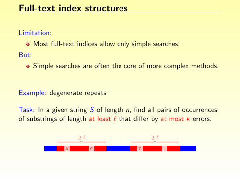
Full-text index structures
Limitation:
Most full-text indices allow only simple searches.
But:
Simple searches are often the core of more complex methods.
Example: degenerate repeats
Task: In a given string S of length n, find all pairs of occurrencesof substrings of length at least ` that differ by at most k errors.
︷ ︸︸ ︷≥ ` ︷ ︸︸ ︷≥ `
C –A G
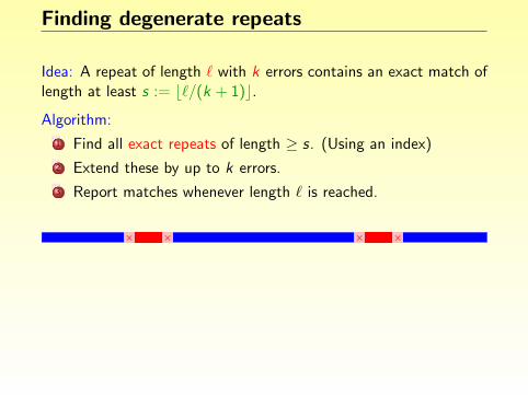
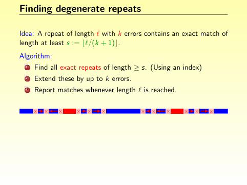
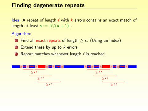
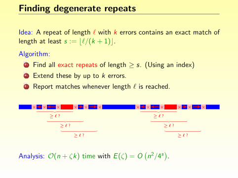
Finding degenerate repeats
Idea: A repeat of length ` with k errors contains an exact match oflength at least s := b`/(k + 1)c.
Algorithm:
1 Find all exact repeats of length ≥ s. (Using an index)
2 Extend these by up to k errors.
3 Report matches whenever length ` is reached.
××××
× × × ×× × × ×
≥ ` ?
≥ ` ?︸ ︷︷ ︸≥ ` ?
︸ ︷︷ ︸ ︸ ︷︷ ︸≥ ` ?︸ ︷︷ ︸
≥ ` ?︸ ︷︷ ︸≥ ` ?
︸ ︷︷ ︸
Analysis: O(n + ζk) time with E (ζ) = O(n2/4s
).

Finding degenerate repeats
Idea: A repeat of length ` with k errors contains an exact match oflength at least s := b`/(k + 1)c.
Algorithm:
1 Find all exact repeats of length ≥ s. (Using an index)
2 Extend these by up to k errors.
3 Report matches whenever length ` is reached.
××××× × × ×
× × × ×
≥ ` ?
≥ ` ?︸ ︷︷ ︸≥ ` ?
︸ ︷︷ ︸ ︸ ︷︷ ︸≥ ` ?︸ ︷︷ ︸
≥ ` ?︸ ︷︷ ︸≥ ` ?
︸ ︷︷ ︸
Analysis: O(n + ζk) time with E (ζ) = O(n2/4s
).
Finding degenerate repeats
Idea: A repeat of length ` with k errors contains an exact match oflength at least s := b`/(k + 1)c.
Algorithm:
1 Find all exact repeats of length ≥ s. (Using an index)
2 Extend these by up to k errors.
3 Report matches whenever length ` is reached.
××××× × × ×× × × ×
≥ ` ?
≥ ` ?︸ ︷︷ ︸≥ ` ?
︸ ︷︷ ︸ ︸ ︷︷ ︸≥ ` ?︸ ︷︷ ︸
≥ ` ?︸ ︷︷ ︸≥ ` ?
︸ ︷︷ ︸
Analysis: O(n + ζk) time with E (ζ) = O(n2/4s
).
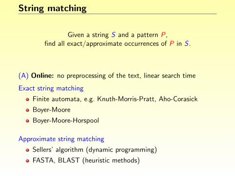
String matching
Given a string S and a pattern P,find all exact/approximate occurrences of P in S .
(A) Online: no preprocessing of the text, linear search time
Exact string matching
Finite automata, e.g. Knuth-Morris-Pratt, Aho-Corasick
Boyer-Moore
Boyer-Moore-Horspool
Approximate string matching
Sellers’ algorithm (dynamic programming)
FASTA, BLAST (heuristic methods)
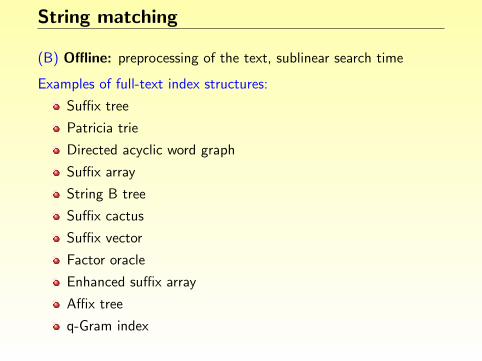
String matching
(B) Offline: preprocessing of the text, sublinear search time
Examples of full-text index structures:
Suffix tree
Patricia trie
Directed acyclic word graph
Suffix array
String B tree
Suffix cactus
Suffix vector
Factor oracle
Enhanced suffix array
Affix tree
q-Gram index

String matching
(B) Offline: preprocessing of the text, sublinear search time
Examples of full-text index structures:
Suffix tree
Patricia trie
Directed acyclic word graph
Suffix array
String B tree
Suffix cactus
Suffix vector
Factor oracle
Enhanced suffix array
Affix tree
q-Gram index
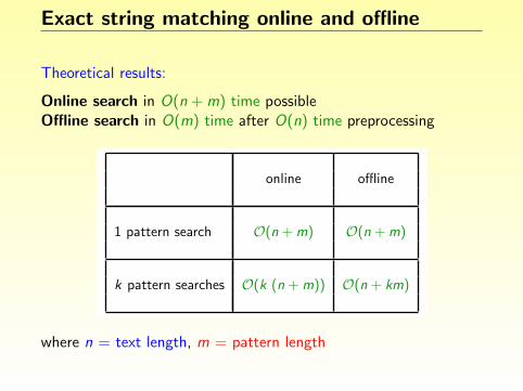
Exact string matching online and offline
Theoretical results:
Online search in O(n + m) time possibleOffline search in O(m) time after O(n) time preprocessing
online offline
1 pattern search O(n + m) O(n + m)
k pattern searches O(k (n + m)) O(n + km)
where n = text length, m = pattern length

Index structures in biological sequence analysis
1 Introduction
2 Suffix trees
3 Affix trees
4 Suffix arrays
5 The q-Gram index
6 Summary and Conclusion

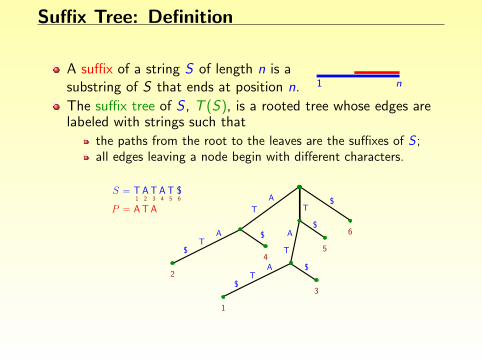
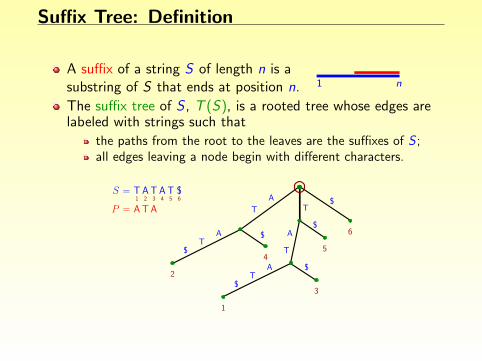
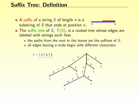
Suffix Tree: Definition
A suffix of a string S of length n is asubstring of S that ends at position n. 1 n
The suffix tree of S , T (S), is a rooted tree whose edges arelabeled with strings such that
the paths from the root to the leaves are the suffixes of S ;all edges leaving a node begin with different characters.
$
1
TS = A T3
A T $65421
2
$T
$
4A
T$
3
5
$
$
6
A
T
A
T
A
T
P = A T AA
T
AA
T
A
P = T A T T T
A
T
T
A
T
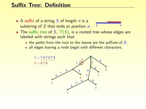
Suffix Tree: Definition
A suffix of a string S of length n is asubstring of S that ends at position n. 1 n
The suffix tree of S , T (S), is a rooted tree whose edges arelabeled with strings such that
the paths from the root to the leaves are the suffixes of S ;all edges leaving a node begin with different characters.
$
1
TS = A T3
A T $65421
2
$T
$
4A
T$
3
5
$
$
6
A
T
A
T
A
T
P = A T A
A
T
AA
T
A
P = T A T T T
A
T
T
A
T
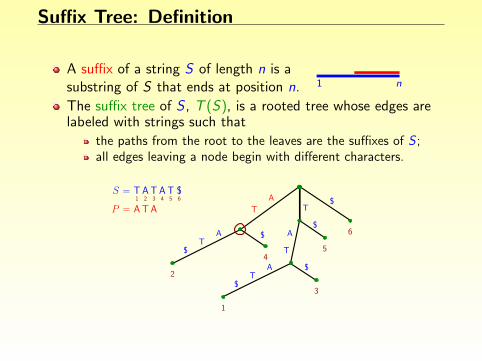
Suffix Tree: Definition
A suffix of a string S of length n is asubstring of S that ends at position n. 1 n
The suffix tree of S , T (S), is a rooted tree whose edges arelabeled with strings such that
the paths from the root to the leaves are the suffixes of S ;all edges leaving a node begin with different characters.
$
1
TS = A T3
A T $65421
2
$T
$
4A
T$
3
5
$
$
6
A
T
A
T
A
T
P = A T A
A
T
AA
T
A
P = T A T T T
A
T
T
A
T
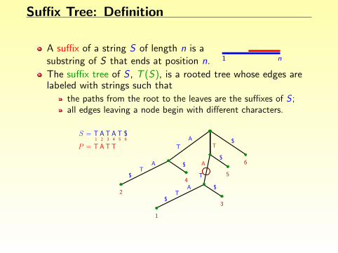
Suffix Tree: Definition
A suffix of a string S of length n is asubstring of S that ends at position n. 1 n
The suffix tree of S , T (S), is a rooted tree whose edges arelabeled with strings such that
the paths from the root to the leaves are the suffixes of S ;all edges leaving a node begin with different characters.
$
1
TS = A T3
A T $65421
2
$T
$
4A
T$
3
5
$
$
6
A
T
A
T
A
T
P = A T AA
T
AA
T
A
P = T A T T T
A
T
T
A
T

Suffix Tree: Definition
A suffix of a string S of length n is asubstring of S that ends at position n. 1 n
The suffix tree of S , T (S), is a rooted tree whose edges arelabeled with strings such that
the paths from the root to the leaves are the suffixes of S ;all edges leaving a node begin with different characters.
$
1
TS = A T3
A T $65421
2
$T
$
4A
T$
3
5
$
$
6
A
T
A
T
A
T
P = A T AA
T
A
A
T
A
P = T A T T
T
A
T
T
A
T

Suffix Tree: Definition
A suffix of a string S of length n is asubstring of S that ends at position n. 1 n
The suffix tree of S , T (S), is a rooted tree whose edges arelabeled with strings such that
the paths from the root to the leaves are the suffixes of S ;all edges leaving a node begin with different characters.
$
1
TS = A T3
A T $65421
2
$T
$
4A
T$
3
5
$
$
6
A
T
A
T
A
T
P = A T AA
T
A
A
T
A
P = T A T T T
A
T
T
A
T
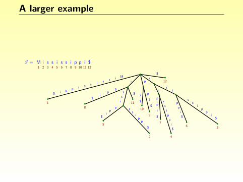
A larger example
S = ss ippiM i s s i987654321 10 11
$12
$
si
ss
ip
pi
$
p
p
i
$
$
i
p
p
i
s
s
i
sp
p
i
$
p
p
i
$
i
$
$
i
Mississippi$
$i
pp
s
s
i
pp
i$
ss
ip
pi
$
1
8
5
4
7
9
10
11
6 3
12
2

Suffix tree properties
T (S) represents exactly the substrings of S .
T (S) allows to enumerate these substrings and their locationsin S in a convenient way.
This is very useful for many pattern recognition problems, forexample:
exact string matching as part of other applications, e.g.detecting DNA contaminationall-pairs suffix-prefix matching, important in fragmentassemblyfinding repeats and palindromes, tandem repeats, degeneraterepeatsDNA primer designDNA chip design...
See also:
A. Apostolico: The myriad virtues of subword trees, 1985.
D. Gusfield: Algorithms on strings, trees, and sequences, 1997.

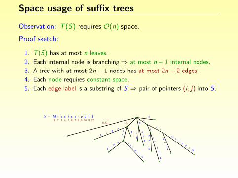
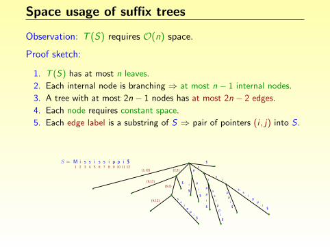
Space usage of suffix trees
Observation: T (S) requires O(n) space.
Proof sketch:
1. T (S) has at most n leaves.
2. Each internal node is branching ⇒ at most n − 1 internal nodes.
3. A tree with at most 2n − 1 nodes has at most 2n − 2 edges.
4. Each node requires constant space.
5. Each edge label is a substring of S ⇒ pair of pointers (i , j) into S .
S = ippississiM1 2 3 4 5 6 7 8 9 10 11
$12 Mis
ssi
sippi$
i
pp
i$
s
s
i
pp
i$
ss
ip
pi
$
$
p
$
i
$
i
p
s
i
$
i
p
p
$
p
i
p
i
s
s
si
p
p
i
$
ss
ip
pi
$
$
(1,12) (2,2)
(9,12)
(6,8)
(9,12)
(6,12)
(12,12)
(9,9)
(11,12) (10,12)
(3,3)
(5,5)
(9,12)
(6,12)
(4,5)
(9,12) (6,12)
(12,12)

Space usage of suffix trees
Observation: T (S) requires O(n) space.
Proof sketch:
1. T (S) has at most n leaves.
2. Each internal node is branching ⇒ at most n − 1 internal nodes.
3. A tree with at most 2n − 1 nodes has at most 2n − 2 edges.
4. Each node requires constant space.
5. Each edge label is a substring of S ⇒ pair of pointers (i , j) into S .
S = ippississiM1 2 3 4 5 6 7 8 9 10 11
$12
Mis
ssi
sippi$
i
pp
i$
s
s
i
pp
i$
ss
ip
pi
$
$
p
$
i
$
i
p
s
i
$
i
p
p
$
p
i
p
i
s
s
si
p
p
i
$
ss
ip
pi
$
$
(1,12)
(2,2)
(9,12)
(6,8)
(9,12)
(6,12)
(12,12)
(9,9)
(11,12) (10,12)
(3,3)
(5,5)
(9,12)
(6,12)
(4,5)
(9,12) (6,12)
(12,12)
Space usage of suffix trees
Observation: T (S) requires O(n) space.
Proof sketch:
1. T (S) has at most n leaves.
2. Each internal node is branching ⇒ at most n − 1 internal nodes.
3. A tree with at most 2n − 1 nodes has at most 2n − 2 edges.
4. Each node requires constant space.
5. Each edge label is a substring of S ⇒ pair of pointers (i , j) into S .
S = ippississiM1 2 3 4 5 6 7 8 9 10 11
$12
Mis
ssi
sippi$
i
pp
i$
s
s
i
pp
i$
ss
ip
pi
$
$
p
$
i
$
i
p
s
i
$
i
p
p
$
p
i
p
i
s
s
si
p
p
i
$
ss
ip
pi
$
$
(1,12) (2,2)
(9,12)
(6,8)
(9,12)
(6,12)
(12,12)
(9,9)
(11,12) (10,12)
(3,3)
(5,5)
(9,12)
(6,12)
(4,5)
(9,12) (6,12)
(12,12)

Space usage of suffix trees
Observation: T (S) requires O(n) space.
Proof sketch:
1. T (S) has at most n leaves.
2. Each internal node is branching ⇒ at most n − 1 internal nodes.
3. A tree with at most 2n − 1 nodes has at most 2n − 2 edges.
4. Each node requires constant space.
5. Each edge label is a substring of S ⇒ pair of pointers (i , j) into S .
S = ippississiM1 2 3 4 5 6 7 8 9 10 11
$12
Mis
ssi
sippi$
i
pp
i$
s
s
i
pp
i$
ss
ip
pi
$
$
p
$
i
$
i
p
s
i
$
i
p
p
$
p
i
p
i
s
s
si
p
p
i
$
ss
ip
pi
$
$
(1,12) (2,2)
(9,12)
(6,8)
(9,12)
(6,12)
(12,12)
(9,9)
(11,12) (10,12)
(3,3)
(5,5)
(9,12)
(6,12)
(4,5)
(9,12) (6,12)
(12,12)

Space usage of suffix trees
Observation: T (S) requires O(n) space.
Proof sketch:
1. T (S) has at most n leaves.
2. Each internal node is branching ⇒ at most n − 1 internal nodes.
3. A tree with at most 2n − 1 nodes has at most 2n − 2 edges.
4. Each node requires constant space.
5. Each edge label is a substring of S ⇒ pair of pointers (i , j) into S .
S = ippississiM1 2 3 4 5 6 7 8 9 10 11
$12
Mis
ssi
sippi$
i
pp
i$
s
s
i
pp
i$
ss
ip
pi
$
$
p
$
i
$
i
p
s
i
$
i
p
p
$
p
i
p
i
s
s
si
p
p
i
$
ss
ip
pi
$
$
(1,12) (2,2)
(9,12)
(6,8)
(9,12)
(6,12)
(12,12)
(9,9)
(11,12)
(10,12)
(3,3)
(5,5)
(9,12)
(6,12)
(4,5)
(9,12) (6,12)
(12,12)

Space usage of suffix trees
Observation: T (S) requires O(n) space.
Proof sketch:
1. T (S) has at most n leaves.
2. Each internal node is branching ⇒ at most n − 1 internal nodes.
3. A tree with at most 2n − 1 nodes has at most 2n − 2 edges.
4. Each node requires constant space.
5. Each edge label is a substring of S ⇒ pair of pointers (i , j) into S .
S = ippississiM1 2 3 4 5 6 7 8 9 10 11
$12
Mis
ssi
sippi$
i
pp
i$
s
s
i
pp
i$
ss
ip
pi
$
$
p
$
i
$
i
p
s
i
$
i
p
p
$
p
i
p
i
s
s
si
p
p
i
$
ss
ip
pi
$
$
(1,12) (2,2)
(9,12)
(6,8)
(9,12)
(6,12)
(12,12)
(9,9)
(11,12) (10,12)
(3,3)
(5,5)
(9,12)
(6,12)
(4,5)
(9,12) (6,12)
(12,12)

Space usage of suffix trees
Observation: T (S) requires O(n) space.
Proof sketch:
1. T (S) has at most n leaves.
2. Each internal node is branching ⇒ at most n − 1 internal nodes.
3. A tree with at most 2n − 1 nodes has at most 2n − 2 edges.
4. Each node requires constant space.
5. Each edge label is a substring of S ⇒ pair of pointers (i , j) into S .
S = ippississiM1 2 3 4 5 6 7 8 9 10 11
$12
Mis
ssi
sippi$
i
pp
i$
s
s
i
pp
i$
ss
ip
pi
$
$
p
$
i
$
i
p
s
i
$
i
p
p
$
p
i
p
i
s
s
si
p
p
i
$
ss
ip
pi
$
$
(1,12) (2,2)
(9,12)
(6,8)
(9,12)
(6,12)
(12,12)
(9,9)
(11,12) (10,12)
(3,3)
(5,5)
(9,12)
(6,12)
(4,5)
(9,12)
(6,12)
(12,12)

Space usage of suffix trees
Observation: T (S) requires O(n) space.
Proof sketch:
1. T (S) has at most n leaves.
2. Each internal node is branching ⇒ at most n − 1 internal nodes.
3. A tree with at most 2n − 1 nodes has at most 2n − 2 edges.
4. Each node requires constant space.
5. Each edge label is a substring of S ⇒ pair of pointers (i , j) into S .
S = ippississiM1 2 3 4 5 6 7 8 9 10 11
$12
Mis
ssi
sippi$
i
pp
i$
s
s
i
pp
i$
ss
ip
pi
$
$
p
$
i
$
i
p
s
i
$
i
p
p
$
p
i
p
i
s
s
si
p
p
i
$
ss
ip
pi
$
$
(1,12) (2,2)
(9,12)
(6,8)
(9,12)
(6,12)
(12,12)
(9,9)
(11,12) (10,12)
(3,3)
(5,5)
(9,12)
(6,12)
(4,5)
(9,12) (6,12)
(12,12)

Space usage of suffix trees
Observation: T (S) requires O(n) space.
Proof sketch:
1. T (S) has at most n leaves.
2. Each internal node is branching ⇒ at most n − 1 internal nodes.
3. A tree with at most 2n − 1 nodes has at most 2n − 2 edges.
4. Each node requires constant space.
5. Each edge label is a substring of S ⇒ pair of pointers (i , j) into S .
S = ippississiM1 2 3 4 5 6 7 8 9 10 11
$12
Mis
ssi
sippi$
i
pp
i$
s
s
i
pp
i$
ss
ip
pi
$
$
p
$
i
$
i
p
s
i
$
i
p
p
$
p
i
p
i
s
s
si
p
p
i
$
ss
ip
pi
$
$
(1,12) (2,2)
(9,12)
(6,8)
(9,12)
(6,12)
(12,12)
(9,9)
(11,12) (10,12)
(3,3)
(5,5)
(9,12)
(6,12)
(4,5)
(9,12) (6,12)
(12,12)
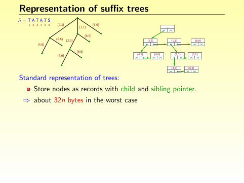
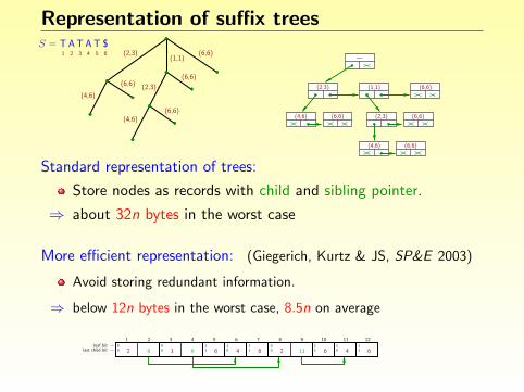
Representation of suffix trees
(6,6)
(6,6)
(6,6)1 2 4 5 63
(4,6)(2,3)(6,6)
(4,6)
(1,1)(2,3)
A T A T $S = T
Standard representation of trees:
Store nodes as records with child and sibling pointer.
⇒ about 32n bytes in the worst case
(4,6) (6,6)
(6,6)
(6,6)(1,1)
(2,3)(6,6)(4,6)
(2,3)
—
More efficient representation: (Giegerich, Kurtz & JS, SP&E 2003)
Avoid storing redundant information.
⇒ below 12n bytes in the worst case, 8.5n on average
6 8 112 1 6 4 6 2 6 4 6
1 2 3 4 5 6 7 8 9 12111011
10
11
00
11
10
11
00
00last child bit →
leaf bit →
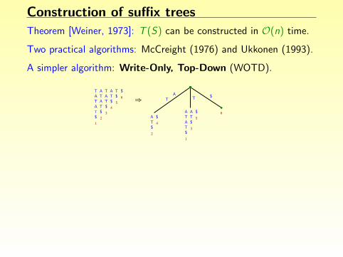
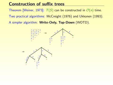
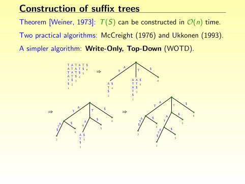
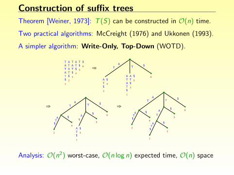
Construction of suffix trees
Theorem [Weiner, 1973]: T (S) can be constructed in O(n) time.
Two practical algorithms: McCreight (1976) and Ukkonen (1993).
A simpler algorithm: Write-Only, Top-Down (WOTD).
T
1
2
3
4
5
6
TATA
$TATA T
AT$
$TA T
$$
$
AT
$AT$
T
$AT$
ATAT$
$
6
5
3
1
4
2
⇒
$T
$A
T
$AT
$AT$
TA
$
1
4
2 3
5
6
⇒T
AT
AT
$ A
T
AT$
$
$
$
$
1
2
3
5
6
4
⇒
Analysis: O(n2) worst-case, O(n log n) expected time, O(n) space
Note: The WOTD algorithm is well suited for a lazy construction.
Construction of suffix trees
Theorem [Weiner, 1973]: T (S) can be constructed in O(n) time.
Two practical algorithms: McCreight (1976) and Ukkonen (1993).
A simpler algorithm: Write-Only, Top-Down (WOTD).
T
1
2
3
4
5
6
TATA
$TATA T
AT$
$TA T
$$
$
AT
$AT$
T
$AT$
ATAT$
$
6
5
3
1
4
2
⇒
$T
$A
T
$AT
$AT$
TA
$
1
4
2 3
5
6
⇒
TA
T
AT
$ A
T
AT$
$
$
$
$
1
2
3
5
6
4
⇒
Analysis: O(n2) worst-case, O(n log n) expected time, O(n) space
Note: The WOTD algorithm is well suited for a lazy construction.
Construction of suffix trees
Theorem [Weiner, 1973]: T (S) can be constructed in O(n) time.
Two practical algorithms: McCreight (1976) and Ukkonen (1993).
A simpler algorithm: Write-Only, Top-Down (WOTD).
T
1
2
3
4
5
6
TATA
$TATA T
AT$
$TA T
$$
$
AT
$AT$
T
$AT$
ATAT$
$
6
5
3
1
4
2
⇒
$T
$A
T
$AT
$AT$
TA
$
1
4
2 3
5
6
⇒T
AT
AT
$ A
T
AT$
$
$
$
$
1
2
3
5
6
4
⇒
Analysis: O(n2) worst-case, O(n log n) expected time, O(n) space
Note: The WOTD algorithm is well suited for a lazy construction.
Construction of suffix trees
Theorem [Weiner, 1973]: T (S) can be constructed in O(n) time.
Two practical algorithms: McCreight (1976) and Ukkonen (1993).
A simpler algorithm: Write-Only, Top-Down (WOTD).
T
1
2
3
4
5
6
TATA
$TATA T
AT$
$TA T
$$
$
AT
$AT$
T
$AT$
ATAT$
$
6
5
3
1
4
2
⇒
$T
$A
T
$AT
$AT$
TA
$
1
4
2 3
5
6
⇒T
AT
AT
$ A
T
AT$
$
$
$
$
1
2
3
5
6
4
⇒
Analysis: O(n2) worst-case, O(n log n) expected time, O(n) space
Note: The WOTD algorithm is well suited for a lazy construction.
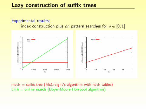
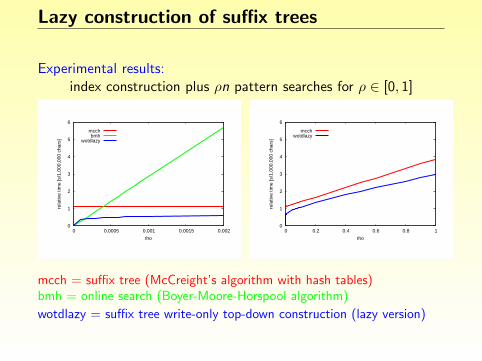
Lazy construction of suffix trees
Experimental results:index construction plus ρn pattern searches for ρ ∈ [0, 1]
0
1
2
3
4
5
6
0 0.0005 0.001 0.0015 0.002
rela
tive
time
[s/1
,000
,000
cha
rs]
rho
mcchbmh
0
1
2
3
4
5
6
0 0.2 0.4 0.6 0.8 1
rela
tive
time
[s/1
,000
,000
cha
rs]
rho
mcch
0
1
2
3
4
5
6
0 0.0005 0.001 0.0015 0.002
rela
tive
time
[s/1
,000
,000
cha
rs]
rho
mcchbmh
wotdlazy
0
1
2
3
4
5
6
0 0.2 0.4 0.6 0.8 1
rela
tive
time
[s/1
,000
,000
cha
rs]
rho
mcchwotdlazy
mcch = suffix tree (McCreight’s algorithm with hash tables)bmh = online search (Boyer-Moore-Horspool algorithm)
wotdlazy = suffix tree write-only top-down construction (lazy version)
Index structures in biological sequence analysis
1 Introduction
2 Suffix trees
3 Affix trees
4 Suffix arrays
5 The q-Gram index
6 Summary and Conclusion
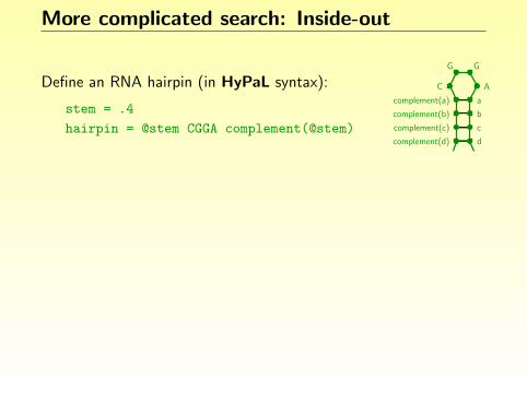
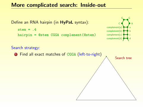
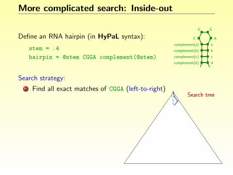
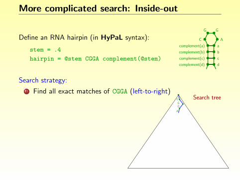
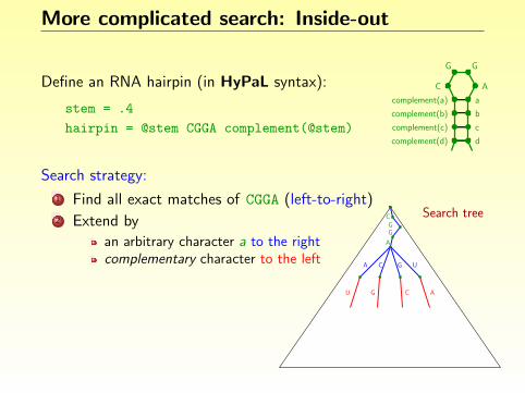
More complicated search: Inside-out
Define an RNA hairpin (in HyPaL syntax):
stem = .4
hairpin = @stem CGGA complement(@stem)
C A
G G
acomplement(a)
b
c
d
complement(b)
complement(c)
complement(d)
Search strategy:
1 Find all exact matches of CGGA (left-to-right)2 Extend by
an arbitrary character a to the rightcomplementary character to the leftan arbitrary character b to the rightcomplementary character to the left. . .
Search treeCGG
A
CA G U
U G C A
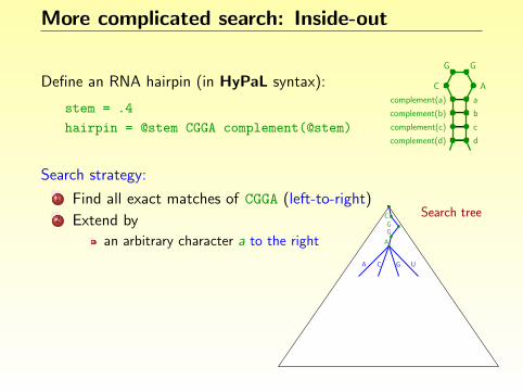
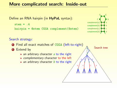
More complicated search: Inside-out
Define an RNA hairpin (in HyPaL syntax):
stem = .4
hairpin = @stem CGGA complement(@stem)
C A
G G
acomplement(a)
b
c
d
complement(b)
complement(c)
complement(d)
Search strategy:
1 Find all exact matches of CGGA (left-to-right)
2 Extend by
an arbitrary character a to the rightcomplementary character to the leftan arbitrary character b to the rightcomplementary character to the left. . .
Search tree
CGG
A
CA G U
U G C A

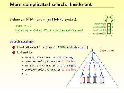
More complicated search: Inside-out
Define an RNA hairpin (in HyPaL syntax):
stem = .4
hairpin = @stem CGGA complement(@stem)
C A
G G
acomplement(a)
b
c
d
complement(b)
complement(c)
complement(d)
Search strategy:
1 Find all exact matches of CGGA (left-to-right)
2 Extend by
an arbitrary character a to the rightcomplementary character to the leftan arbitrary character b to the rightcomplementary character to the left. . .
Search treeC
GG
A
CA G U
U G C A

More complicated search: Inside-out
Define an RNA hairpin (in HyPaL syntax):
stem = .4
hairpin = @stem CGGA complement(@stem)
C A
G G
acomplement(a)
b
c
d
complement(b)
complement(c)
complement(d)
Search strategy:
1 Find all exact matches of CGGA (left-to-right)
2 Extend by
an arbitrary character a to the rightcomplementary character to the leftan arbitrary character b to the rightcomplementary character to the left. . .
Search treeCG
G
A
CA G U
U G C A
More complicated search: Inside-out
Define an RNA hairpin (in HyPaL syntax):
stem = .4
hairpin = @stem CGGA complement(@stem)
C A
G G
acomplement(a)
b
c
d
complement(b)
complement(c)
complement(d)
Search strategy:
1 Find all exact matches of CGGA (left-to-right)
2 Extend by
an arbitrary character a to the rightcomplementary character to the leftan arbitrary character b to the rightcomplementary character to the left. . .
Search treeCGG
A
CA G U
U G C A
More complicated search: Inside-out
Define an RNA hairpin (in HyPaL syntax):
stem = .4
hairpin = @stem CGGA complement(@stem)
C A
G G
acomplement(a)
b
c
d
complement(b)
complement(c)
complement(d)
Search strategy:
1 Find all exact matches of CGGA (left-to-right)2 Extend by
an arbitrary character a to the right
complementary character to the leftan arbitrary character b to the rightcomplementary character to the left. . .
Search treeCGG
A
CA G U
U G C A
More complicated search: Inside-out
Define an RNA hairpin (in HyPaL syntax):
stem = .4
hairpin = @stem CGGA complement(@stem)
C A
G G
acomplement(a)
b
c
d
complement(b)
complement(c)
complement(d)
Search strategy:
1 Find all exact matches of CGGA (left-to-right)2 Extend by
an arbitrary character a to the rightcomplementary character to the left
an arbitrary character b to the rightcomplementary character to the left. . .
Search treeCGG
A
CA G U
U G C A
More complicated search: Inside-out
Define an RNA hairpin (in HyPaL syntax):
stem = .4
hairpin = @stem CGGA complement(@stem)
C A
G G
acomplement(a)
b
c
d
complement(b)
complement(c)
complement(d)
Search strategy:
1 Find all exact matches of CGGA (left-to-right)2 Extend by
an arbitrary character a to the rightcomplementary character to the leftan arbitrary character b to the right
complementary character to the left. . .
Search treeCGG
A
CA G U
U G C A

More complicated search: Inside-out
Define an RNA hairpin (in HyPaL syntax):
stem = .4
hairpin = @stem CGGA complement(@stem)
C A
G G
acomplement(a)
b
c
d
complement(b)
complement(c)
complement(d)
Search strategy:
1 Find all exact matches of CGGA (left-to-right)2 Extend by
an arbitrary character a to the rightcomplementary character to the leftan arbitrary character b to the rightcomplementary character to the left
. . .
Search treeCGG
A
CA G U
U G C A
More complicated search: Inside-out
Define an RNA hairpin (in HyPaL syntax):
stem = .4
hairpin = @stem CGGA complement(@stem)
C A
G G
acomplement(a)
b
c
d
complement(b)
complement(c)
complement(d)
Search strategy:
1 Find all exact matches of CGGA (left-to-right)2 Extend by
an arbitrary character a to the rightcomplementary character to the leftan arbitrary character b to the rightcomplementary character to the left. . .
Search treeCGG
A
CA G U
U G C A

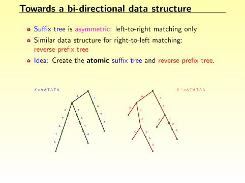
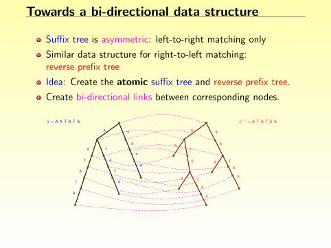
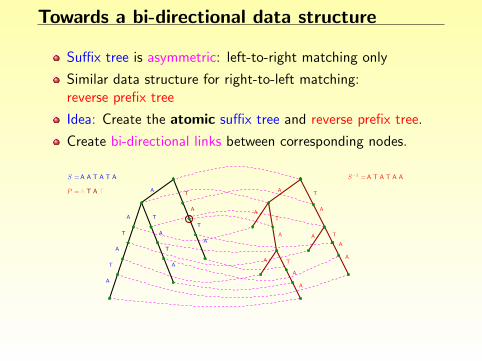
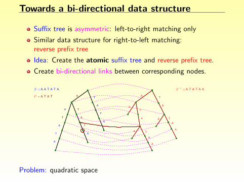
Towards a bi-directional data structure
Suffix tree is asymmetric: left-to-right matching only
Similar data structure for right-to-left matching:reverse prefix tree
Idea: Create the atomic suffix tree and reverse prefix tree.
Create bi-directional links between corresponding nodes.
A
T
A
A
T
A
T
A
S =A A T A T A
T
A
T
A
T
AT
A
T
A
A
A
A
A T
A
A
AATATAS−1 =
T
A
A
P = T AA TT TA
A
TA A
T
A
T
T
A
T
A
Problem: quadratic space

Towards a bi-directional data structure
Suffix tree is asymmetric: left-to-right matching only
Similar data structure for right-to-left matching:reverse prefix tree
Idea: Create the atomic suffix tree and reverse prefix tree.
Create bi-directional links between corresponding nodes.
A
T
A
A
T
A
T
A
S =A A T A T A
T
A
T
A
T
AT
A
T
A
A
A
A
A T
A
A
AATATAS−1 =
T
A
A
P = T AA T
T TA
A
TA A
T
A
T
T
A
T
A
Problem: quadratic space

Towards a bi-directional data structure
Suffix tree is asymmetric: left-to-right matching only
Similar data structure for right-to-left matching:reverse prefix tree
Idea: Create the atomic suffix tree and reverse prefix tree.
Create bi-directional links between corresponding nodes.
A
T
A
A
T
A
T
A
S =A A T A T A
T
A
T
A
T
AT
A
T
A
A
A
A
A T
A
A
AATATAS−1 =
T
A
A
P =
T
AA TT T
A
A
TA A
T
A
T
T
A
T
A
Problem: quadratic space
Towards a bi-directional data structure
Suffix tree is asymmetric: left-to-right matching only
Similar data structure for right-to-left matching:reverse prefix tree
Idea: Create the atomic suffix tree and reverse prefix tree.
Create bi-directional links between corresponding nodes.
A
T
A
A
T
A
T
A
S =A A T A T A
T
A
T
A
T
AT
A
T
A
A
A
A
A T
A
A
AATATAS−1 =
T
A
A
P =
T A
A TT
T
A
A
T
A A
T
A
T
T
A
T
A
Problem: quadratic space

Towards a bi-directional data structure
Suffix tree is asymmetric: left-to-right matching only
Similar data structure for right-to-left matching:reverse prefix tree
Idea: Create the atomic suffix tree and reverse prefix tree.
Create bi-directional links between corresponding nodes.
A
T
A
A
T
A
T
A
S =A A T A T A
T
A
T
A
T
AT
A
T
A
A
A
A
A T
A
A
AATATAS−1 =
T
A
A
P =
T AA
TT
T
A
A
T
A A
T
A
T
T
A
T
A
Problem: quadratic space

Towards a bi-directional data structure
Suffix tree is asymmetric: left-to-right matching only
Similar data structure for right-to-left matching:reverse prefix tree
Idea: Create the atomic suffix tree and reverse prefix tree.
Create bi-directional links between corresponding nodes.
A
T
A
A
T
A
T
A
S =A A T A T A
T
A
T
A
T
A
T
A
T
A
A
A
A
A T
A
A
AATATAS−1 =
T
A
A
P =
T AA T
T
T
A
A
T
A
A
T
A
T
T
A
T
A
Problem: quadratic space
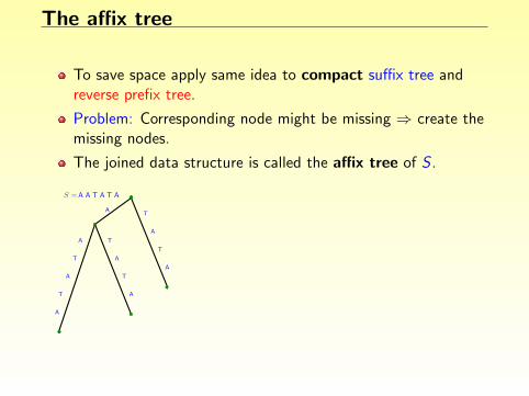
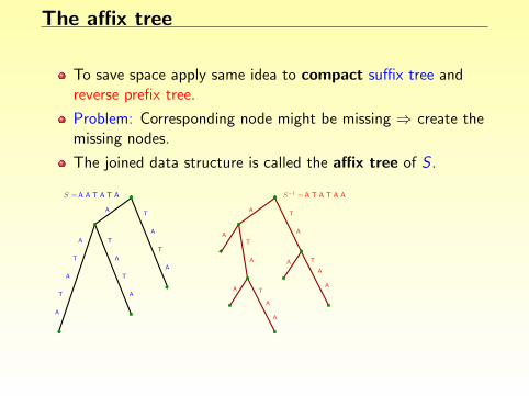
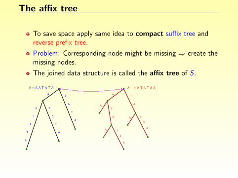
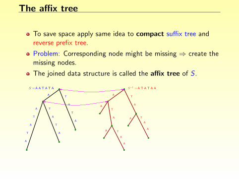
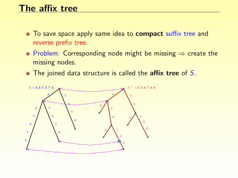
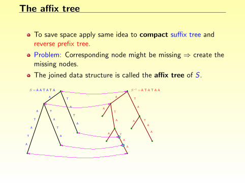
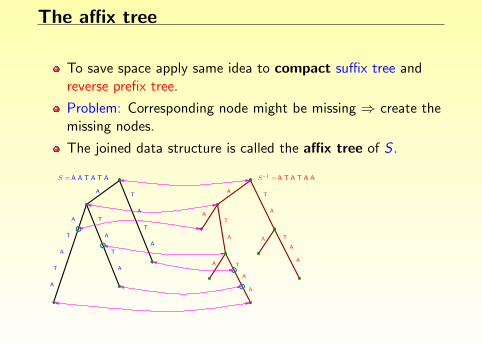
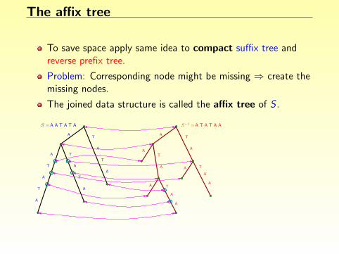
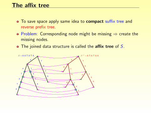
The affix tree
To save space apply same idea to compact suffix tree andreverse prefix tree.
Problem: Corresponding node might be missing ⇒ create themissing nodes.
The joined data structure is called the affix tree of S .
T
A
A
T
T
A
T
A
A
T
A
T
A
A
S =A A T A T A
T
A
T
A
A
A
AT
A T
A
A
A
A
AATATAS−1 =
A
A
A
A
T
T
A
T
A
TA
A
A
T
T
T
A
T
A
A
AT
A
A
A
AA
T
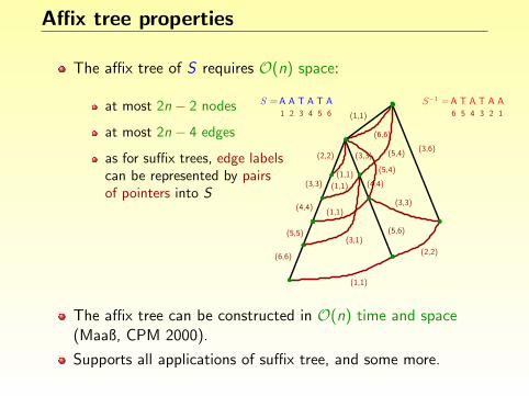
Affix tree properties
The affix tree of S requires O(n) space:
at most 2n − 2 nodes
at most 2n − 4 edges
as for suffix trees, edge labelscan be represented by pairsof pointers into S
S =A A T A T A1 2 3 4 5 6
AATATAS−1 =12345
(5,4)
6
(6,6)
(3,6)
(2,2)
(4,4)
(3,3)
(2,2)
(1,1)
(1,1)
(1,1)
(1,1)
(5,6)(3,1)
(4,4)
(3,3)
(3,3)
(5,4)
(6,6)
(5,5)
(1,1)
The affix tree can be constructed in O(n) time and space(Maaß, CPM 2000).
Supports all applications of suffix tree, and some more.
Index structures in biological sequence analysis
1 Introduction
2 Suffix trees
3 Affix trees
4 Suffix arrays
5 The q-Gram index
6 Summary and Conclusion
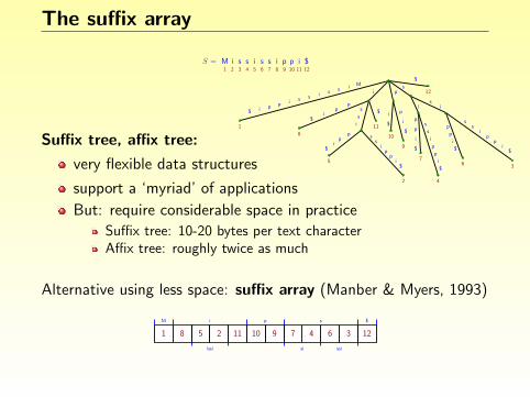
The suffix array
S = ss ippiM i s s i987654321 10 11
$12
$
si
ss
ip
pi
$
p
p
i
$
$
i
p
p
i
s
s
i
sp
p
i
$
p
p
i
$
i
$
$
i
Mississippi$
$i
pp
s
s
i
pp
i$
ss
ip
pi
$
1
8
5
4
7
9
10
11
6 3
12
2
Suffix tree, affix tree:
very flexible data structures
support a ‘myriad’ of applications
But: require considerable space in practice
Suffix tree: 10-20 bytes per text characterAffix tree: roughly twice as much
Alternative using less space: suffix array (Manber & Myers, 1993)
M i p s $
issi si ssi
123647910112581
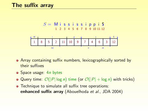
The suffix array
S = ss ippiM i s s i987654321 10 11
$12
M i p s $
issi si ssi
123647910112581
Array containing suffix numbers, lexicographically sorted bytheir suffixes
Space usage: 4n bytes
Query time: O(|P| log n) time (or O(|P|+ log n) with tricks)
Technique to simulate all suffix tree operations:enhanced suffix array (Abouelhoda et al., JDA 2004)
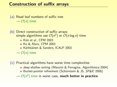
Construction of suffix arrays
(a) Read leaf numbers of suffix tree→ O(n) time
(b) Direct construction of suffix arrays:simple algorithms use O(n2) or O(n log n) time
Kim et al., CPM 2003Ko & Aluru, CPM 2003Karkkainen & Sanders, ICALP 2003
→ O(n) time
(c) Practical algorithms have worse time complexities
deep shallow sorting (Manzini & Ferragina, Algorithmica 2004)Bucket-pointer refinement (Schurmann & JS, SP&E 2006)
→ O(n2) time in worst case, much better in practice
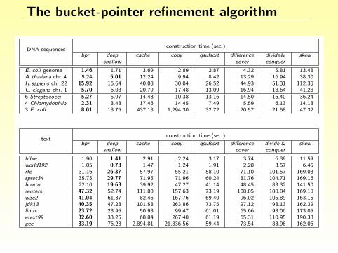
The bucket-pointer refinement algorithm
DNA sequencesconstruction time (sec.)
bpr deep cache copy qsufsort difference divide& skewshallow cover conquer
E. coli genome 1.46 1.71 3.69 2.89 2.87 4.32 5.81 13.48A. thaliana chr. 4 5.24 5.01 12.24 9.94 8.42 13.29 16.94 38.30H.sapiens chr.22 15.92 16.64 40.08 30.04 26.52 44.93 51.31 112.38C. elegans chr. 1 5.70 6.03 20.79 17.48 13.09 16.94 18.64 41.286 Streptococci 5.27 5.97 14.43 10.38 13.16 14.50 16.40 36.244 Chlamydophila 2.31 3.43 17.46 14.45 7.49 5.59 6.13 14.133 E. coli 8.01 13.75 437.18 1,294.30 32.72 20.57 21.58 47.32
textconstruction time (sec.)
bpr deep cache copy qsufsort difference divide & skewshallow cover conquer
bible 1.90 1.41 2.91 2.24 3.17 3.74 6.39 11.59world192 1.05 0.73 1.47 1.24 1.91 2.28 3.57 6.45rfc 31.16 26.37 57.97 55.21 58.10 71.10 101.57 169.03sprot34 35.75 29.77 71.95 71.96 60.24 81.76 104.71 169.16howto 22.10 19.63 39.92 47.27 41.14 48.45 83.32 141.50reuters 47.32 52.74 111.80 157.63 73.19 108.85 108.84 169.18w3c2 41.04 61.37 82.46 167.76 69.40 96.02 105.89 163.15jdk13 40.35 47.23 101.58 263.86 73.75 97.12 98.13 162.39linux 23.72 23.95 50.93 99.47 61.01 65.66 98.06 173.05etext99 32.60 33.25 68.84 267.48 61.19 65.31 110.95 190.33gcc 33.19 76.23 2,894.81 21,836.56 59.44 73.54 83.96 162.06
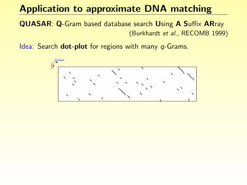
Application to approximate DNA matching
QUASAR: Q-Gram based database search Using A Suffix ARray(Burkhardt et al., RECOMB 1999)
Idea: Search dot-plot for regions with many q-Grams.
query
database
Use suffix array to locate all occurrences of a q-Gram in the database S :
A
A
A
A
A
A
A A
A
A
A
A
C
G
T
C
C G
T T T
suffix array of S
︸ ︷︷ ︸ . . . ︸ ︷︷ ︸︸︷︷︸︸ ︷︷ ︸︸ ︷︷ ︸︸ ︷︷ ︸︸ ︷︷ ︸
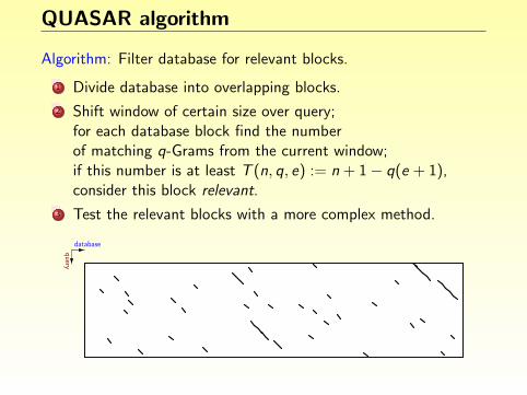
QUASAR algorithm
Algorithm: Filter database for relevant blocks.
1 Divide database into overlapping blocks.
2 Shift window of certain size over query;for each database block find the numberof matching q-Grams from the current window;if this number is at least T (n, q, e) := n + 1− q(e + 1),consider this block relevant.
3 Test the relevant blocks with a more complex method.
query
database
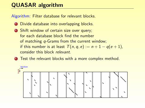
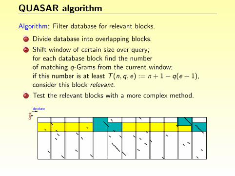
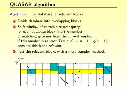
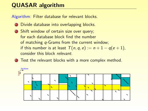
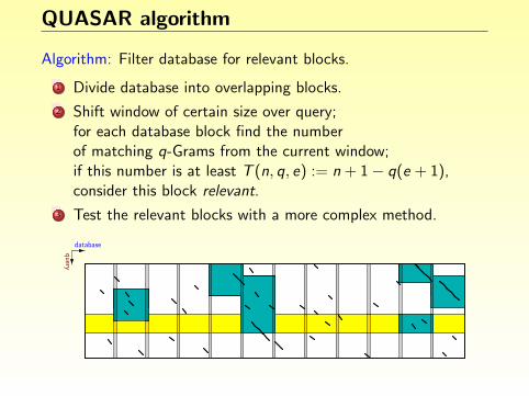
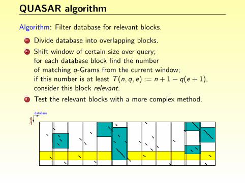
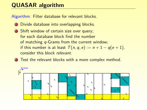
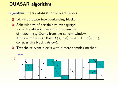
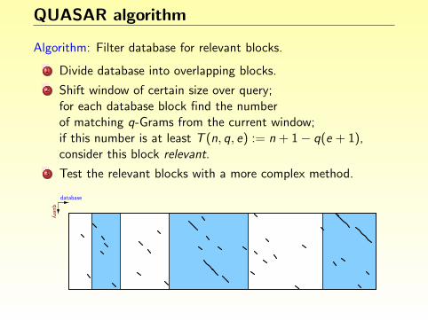

Two ideas for improving QUASAR(Rasmussen, JS & Myers, JCB 2006)
1 Use a simpler index structure: q-Gram indexA
A
A
A
A
A
A A
A
A
A
A
C
G
T
C
C C
T T T
3
5
39
1
11
35
22
92
171
49
4 38
71
110
77
72
33 34
79
158
122
46 47
201
103
63
48 91 121 157 200
113 174 182
94 13132
21
27
Analysis: simple O(n) construction time
2 Reduce size of the relevant regions: parallelograms
query
database
→ need proper filter criteria
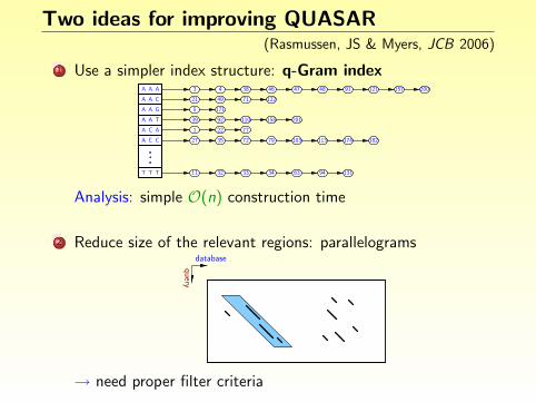
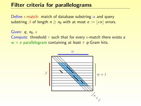
Filter criteria for parallelograms
Define ε-match: match of database substring α and querysubstring β of length n ≥ n0 with at most e := bεnc errors.
Given: q, n0, εCompute: threshold τ such that for every ε-match there exists aw × e parallelogram containing at least τ q-Gram hits.
α
β
}e +
1
w + 1
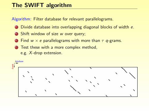
The SWIFT algorithm
Algorithm: Filter database for relevant parallelograms.
1 Divide database into overlapping diagonal blocks of width e.
2 Shift window of size w over query;
3 Find w × e parallelograms with more than τ q-grams.
4 Test these with a more complex method,e.g. X -drop extension.
query
database
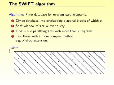
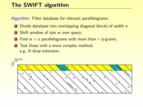
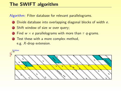
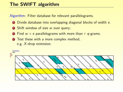
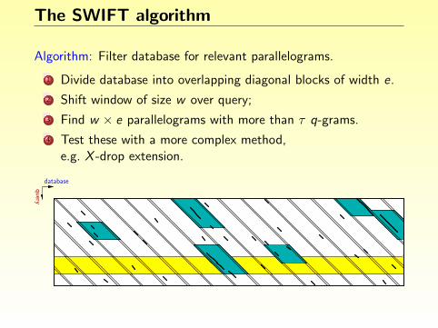
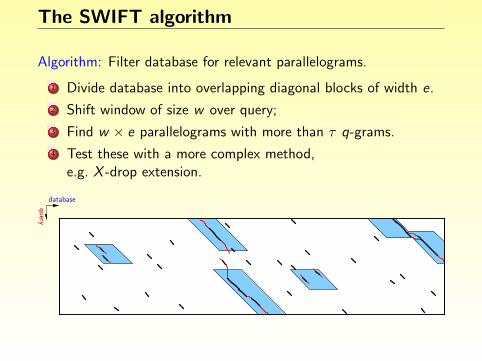

Experimental results
SSEARCH BLASTN SWIFTparameters (ε, n0) — — (5%, 50) (4%, 30) (5%, 30)running time 8h 773 s 18 s 29 s 35 sfiltration ratio — — 6.5e-6 4.5e-6 5.4e-6
Index structures in biological sequence analysis
1 Introduction
2 Suffix trees
3 Affix trees
4 Suffix arrays
5 The q-Gram index
6 Summary and Conclusion
Summary and Conclusion
Handling large amounts of DNA sequence data is challenging
Standard methods do not apply in bioinformatics
Data structures discussed: suffix tree, affix tree, suffix array,q-Gram index
Popular approach: filtration
Tools that use index structures: MUMmer, Genalyzer,SSAHA, BLAT, SWIFT, PatternHunter, ...
Simplicity is often a key element of practical algorithms!
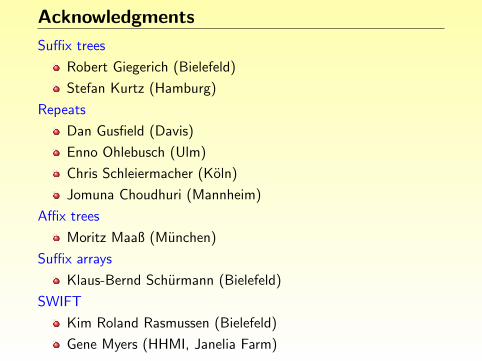
Acknowledgments
Suffix trees
Robert Giegerich (Bielefeld)
Stefan Kurtz (Hamburg)
Repeats
Dan Gusfield (Davis)
Enno Ohlebusch (Ulm)
Chris Schleiermacher (Koln)
Jomuna Choudhuri (Mannheim)
Affix trees
Moritz Maaß (Munchen)
Suffix arrays
Klaus-Bernd Schurmann (Bielefeld)
SWIFT
Kim Roland Rasmussen (Bielefeld)
Gene Myers (HHMI, Janelia Farm)
The end.