index theory of di erential operatorsjfdavis/teaching/m721/mano.pdf · index theory of di erential...
TRANSCRIPT

Index Theory of Differential Operators
Notes prepared and typed byP. Manoharan
Penn State University
Based on lectures given byProf. Dan Burghelea
Department of MathematicsThe Ohio State University
Columbus, Ohio 43210
(PRELIMINARY INCOMPLETE VERSION)
January 8, 2009

Contents
1 De Rham Cohomology 11.1 Introduction . . . . . . . . . . . . . . . . . . . . . . . . . 11.2 Poincare lemma . . . . . . . . . . . . . . . . . . . . . . . 51.3 Thom’s isomorphism . . . . . . . . . . . . . . . . . . . . 61.4 Mayer-Vietories Sequence . . . . . . . . . . . . . . . . . 81.5 Kunneth formula . . . . . . . . . . . . . . . . . . . . . . 101.6 Poincare duality . . . . . . . . . . . . . . . . . . . . . . . 101.7 Compact vertical cohomology . . . . . . . . . . . . . . . 12
2 Vector Fields and Lie Derivatives 172.1 Vector fields . . . . . . . . . . . . . . . . . . . . . . . . . 172.2 Lie derivative . . . . . . . . . . . . . . . . . . . . . . . . 202.3 Cohomology of Lie Groups and Lie Algebras . . . . . . . 212.4 Cohomology of GL(V) . . . . . . . . . . . . . . . . . . . 252.5 Cohomology of Grk(C
n) . . . . . . . . . . . . . . . . . . 27
3 S1 - Equivariant Cohomologies 313.1 Cohomologies on S1-manifolds . . . . . . . . . . . . . . . 31
4 Characteristic Classes and Transfer 414.1 Degree of a map . . . . . . . . . . . . . . . . . . . . . . . 414.2 Lefschetz number of a map . . . . . . . . . . . . . . . . . 424.3 Euler class . . . . . . . . . . . . . . . . . . . . . . . . . . 434.4 Thom’s class . . . . . . . . . . . . . . . . . . . . . . . . . 434.5 Chern classes . . . . . . . . . . . . . . . . . . . . . . . . 454.6 Transfer in a bundle . . . . . . . . . . . . . . . . . . . . 504.7 Generalization of Transfer . . . . . . . . . . . . . . . . . 52
1

2 CONTENTS
5 Connection and Curvature 555.1 Introduction . . . . . . . . . . . . . . . . . . . . . . . . . 555.2 Chern-Weil Formula . . . . . . . . . . . . . . . . . . . . 59
6 Differential Operators and Symbols 656.1 Differential Operators . . . . . . . . . . . . . . . . . . . . 656.2 Symbols . . . . . . . . . . . . . . . . . . . . . . . . . . . 696.3 Elliptic differential Operators . . . . . . . . . . . . . . . 73
7 K-Theory 757.1 Definition of K(X) . . . . . . . . . . . . . . . . . . . . . 757.2 Definition of K(X,Y) . . . . . . . . . . . . . . . . . . . . 76
8 Index of Differential Operators 798.1 Basic Definitions . . . . . . . . . . . . . . . . . . . . . . 798.2 Index on Trivial Bundles . . . . . . . . . . . . . . . . . . 838.3 Index of the de Rham Operator . . . . . . . . . . . . . . 858.4 Index of Dolbeault Operator . . . . . . . . . . . . . . . . 88
9 Signature Operator 959.1 Linear Algebra . . . . . . . . . . . . . . . . . . . . . . . 959.2 Clifford Algebra . . . . . . . . . . . . . . . . . . . . . . . 969.3 The Operator δ . . . . . . . . . . . . . . . . . . . . . . . 979.4 Levi-Civita Connection . . . . . . . . . . . . . . . . . . . 989.5 Topological Index of Signature Operator . . . . . . . . . 103
10 Dirac Operator 10910.1 The Spin Groups . . . . . . . . . . . . . . . . . . . . . . 10910.2 The Spin Structure . . . . . . . . . . . . . . . . . . . . . 11410.3 Topological Index of Dirac Operator . . . . . . . . . . . 11910.4 Twisted Dirac Operator . . . . . . . . . . . . . . . . . . 122
11 Heat Equation Proof 12511.1 Elementary linear algebra . . . . . . . . . . . . . . . . . 12511.2 Super Trace . . . . . . . . . . . . . . . . . . . . . . . . . 128

Chapter 1
De Rham Cohomology
1.1 Introduction
Let A =⊕Ai be a commutative differential graded algebra over K (K
is a field of characteristic zero; in our case K will be either real numbersor complex numbers) where the commutativity means:
a.b = (−1)|a||b|b.a
when a ∈ A|a|, b ∈ B|b| and differential d is a K-linear map of degree 1such that
1. d2 = 0.
2. d(a.b) = (da).b+ (−1)|a|a.(db).
Define
H i(A, d) = Ker(d : Ai → Ai+1)/Im(d : Ai−1 → Ai)
The multiplication induces the linear maps
(kerd)i ⊗ (kerd)j −→ (kerd)i+j
(Imd)i ⊗ (kerd)j −→ (Imd)i+j
For if a = d(c), c ∈ A|c| and d(b) = 0 then
d(c.b) = d(c).b+ (−1)|c|c.d(b) = d(c).b = a.b
1

2 Ch 1: DE RHAM COHOMOLOGY
Therefore we have the multiplication map:
H i(A, d)⊗Hj(A, d) −→ H i+j(A, d)
which makes⊕H i(A, d) into a commutative graded algebra.
Definition 1.1.1 A morphism f : (A, dA) −→ (B, dB) is a collectionof linear maps f i : Ai −→ Bii≥0 such that
1. f idA = dBfi−1 and
2. f i(a.b) = f i(a).f i(b).
If only (1) is satisfied, then f is called a morphism of cochain com-plexes. If f is a morphism of cochain complexes then f induces ahomomorphism
H∗(f) : H∗(A, dA) −→ H∗(B, dB).
If f is a morphism, then H∗(f) defines a homomorphism of commu-tative graded algebra. Sometimes we may also use the notation f ∗ todenote this homomorphism.
Example(1): Let Ω∗ be the algebra generated by dx1, . . . , dxn overR. i.e. Ω∗ = exterior algebra of Rn = Λ(Rn). Thus
Ωr = 〈dxi1 ∧ dxi2 ∧ . . . ∧ dxir | 1 ≤ i1 < i2 < . . . < ir ≤ n〉.
The multiplication is defined by
Ωr ⊗ Ωs −→ Ωr+s
(dxi1 ∧ dxi2 ∧ . . .∧ dxir) · (dxj1 ∧ dxj2 ∧ . . .∧ dxjs) 7−→ (dxi1 ∧ · · · ∧ dxjs)
with the convention that (dxi ∧ dxj) = −(dxj ∧ dxi).Let U ⊆ Rn. Define
Ω∗(U) = C∞(U)⊗ Ω∗
andΩ∗c(U) = C∞c (U)⊗ Ω∗

1.1. INTRODUCTION 3
i.e. Ωr(U) = ∑
1≤i1<i2<···<ir≤nωi1···ir(~x)dxi1 ∧ . . . ∧ dxir
where ωi1···ir(~x) ∈ C∞(U).
d(∑
ωi1···irdxi1 ∧ . . . ∧ dxir) = dw ∧ dxi1 ∧ . . . ∧ dxir
where dω =∑ni=1
∂ω∂xidxi.
Similar definition holds for Ωrc(U).
Definition 1.1.2Hr(U) = Hr(Ω∗(U), d)
andHrc (U) = Hr(Ω∗c(U), d).
Let U,V be open subsets of Rn and Rm respectively. Any smoothmap f : U −→ V induces a map f ∗ : Ω∗(V ) −→ Ω∗(U) by
f ∗(∑
ωi1···ir(~y)dyi1 ∧ . . . ∧ dyir) =∑ωi1···ir(f1(~x), · · · , fm(~x))dfi1 ∧ . . . ∧ dfir
where dfi =∑nj=1
∂fi∂xjdxj and hence we have the homomorphism
H∗(f) : H∗(V ) −→ H∗(U).
Example(2): Let U be an open subset of Rn and G be a Lie group.
µ : G× U → U
be a smooth action and for any fixed g ∈ G,
µg : U → U
u 7→ µ(g, u)
induces µ∗g : Ω∗(U) −→ Ω∗(U).
ΩrG(U) = ω ∈ Ωr(U) | µrg(ω) = ω,∀g ∈ G
Ω∗G(U) is a commutative differential graded algebra.

4 Ch 1: DE RHAM COHOMOLOGY
Example(3): Suppose that U is an open subset of Rn and
µ : R× U −→ U
is a smooth action. Then consider the vector field (refer 2.1)
X =n∑i=1
ai(~x)∂
∂xi
where
ai(~x) =dµidt
(t, ~x) |t=0
The contraction along X is the linear map
iX : Ωr(U) −→ Ωr−1(U)
such that
1. iX(f.ω) = f.iX(ω).
2. iX(ω1 ∧ ω2) = iX(ω1) ∧ ω2 + (−1)|ω1|ω1 ∧ iX(ω2).
3. iX(dxi) = ai(x).
The map LX : Ωi(U) −→ Ωi(U) defined by
LX = diX + iXd
is called Lie derivative.Define Ω∗invX(U) = ω ∈ Ω∗(U) | LXω = 0.
Exercise 1.1.3 Let µ : R × U → U be a smooth action and X be theassociated vector field. Then
Ω∗R(U) = Ω∗invX(U).
Definition 1.1.4 We say that the morphisms
f, g : (A, dA) −→ (B, dB)
(of cochain complexes) are homotopic if there exists a collection of K-linear maps H i : Ai −→ Bi−1 such that
HdA ± dBH = ±(f − g).
If f and g are homotopic then H∗(f) = H∗(g).

1.2. POINCARE LEMMA 5
1.2 Poincare lemma
Let U be an open subset of Rn. Define the maps
π : U ×R→ U
(u, t) 7→ u
sλ : U → (U ×R)
u 7→ (u, λ)
for a fixed λ ∈ R.Obviously π sλ = idU . We have the induced maps
s∗λ : Ω∗(U ×R) −→ Ω∗(U)
π∗ : Ω∗(U ×R)←− Ω∗(U)
such that s∗λ π∗ = id.
Theorem 1.2.1 (Poincare Lemma) id and π∗ s∗λ are homotopic.
Proof: Define the homotopy
Kr : Ωr(U ×R)→ Ωr−1(U ×R)
such that Kd− dK = ±(id− π∗ s∗λ) as follows:Let ω = ω′dxi1 · · · dxir + ω′′dxj1 . . . dxjr−1dt
K(ω)(~x, t) = ∫ t
λω′′(~x, s)dsdxj1 . . . dxjr−1 .
Now dω = dxω + dtω where
dxω =∑i
∂ω′
∂xidxidxi1 . . . dxir +
∑i
∂ω′′
∂xidxidxj1 . . . dxjr−1dt
and
dtω = (−1)r∂ω
∂tdxi1 . . . dxirdt.
Check that Kdω − dKω = ±(ω − π∗ s∗λω).
Corollary 1.2.2
H∗(Rn) =
R if ∗ = 00 if ∗ 6= 0

6 Ch 1: DE RHAM COHOMOLOGY
1.3 Thom’s isomorphism
Define π∗ : Ω∗c(U ×R) −→ Ω∗−1c (U) by∑
ω′i1···ir(~x, t)dxi1 · · · dxir +∑
ω′′j1···jr−1(~x, t)dxj1 · · · dxjr−1dt
7−→∑∫ ∞−∞
ω′′j1···jr−1(~x, t)dtdxj1 · · · dxjr−1
Note: π∗ is not a morphism of differential graded algebra but is a mor-phism of cochain complexes.Choose f ∈ C∞c (R) such that
∫∞−∞ f = 1 and define
ef∗ : Ω∗−1c (U)→ Ω∗c(U ×R)
by ω 7→ fω ∧ dt which is again a morphism of cochain complexes.Usually we will simply write e∗ instead of ef∗ .
We have π∗ e∗ = id.
Theorem 1.3.1 id and e∗ π∗ are homotopic.
Proof: Define
K : Ωrc(U ×R)→ Ωr−1
c (U ×R)
such that
dK −Kd = ±(id− e∗ π∗)
as follows: Let
ω = ω′dxi1 · · · dxir + ω′′dxj1 · · · dxjr−1dt
K(ω)(~x, t) = ∫ t
−∞ω′′(~x, s)dsdxj1 · · · dxjr−1
− ∫ ∞−∞
ω′′(~x, s)ds∫ t
−∞f(s)dsdxj1 · · · dxjr−1
We leave as an exercise to verify that
Kdω − dKω = ±(ω − e∗ π∗(ω)).

1.3. THOM’S ISOMORPHISM 7
Corollary 1.3.2
H∗c (Rn) =
R if ∗ = n0 if ∗ 6= n
Let G acts smoothly on U where G is a compact connected Liegroup with the measure of G is equal to 1. Let µ : G× U → U be thesmooth action of G on U. We have
Ω∗G(U)I→ Ω∗(U)
A→ Ω∗G(U)
where A is defined as follows: Let ω ∈ Ω∗(U)
A(ω) =∫Gµ∗g(ω).
Obviously A I = id. i.e. if ω ∈ Ω∗G then
A I(ω) =∫Gµ∗g(ω) =
∫Gω = ω.
Both I and A are morphism of cochain complexes while I is also amorphism of differential graded algebra.
Exercise 1.3.3 A(dω) = dA(ω).
Theorem 1.3.4 I and A induce isomorphisms for cohomology (Actu-ally I A is homotopic to the identity).
Proof: Exercise (See next chapter).
Corollary 1.3.5 H∗(Ω∗(U), d) ∼= H∗(Ω∗G(U), d).
Remark: If f : U → V is a proper map then f induces
f ∗ : Ω∗c(V )→ Ω∗c(U)
and hence
H∗(f) : H∗c (V )→ H∗c (U).

8 Ch 1: DE RHAM COHOMOLOGY
1.4 Mayer-Vietories Sequence
Let U = U1 ∪ U2. We have a short exact sequence
0→ Ω∗(U)i∗1⊕i
∗2→ Ω∗(U1)⊕ Ω∗(U2)
j∗1−j∗2→ Ω∗(U1 ∩ U2)→ 0
which induces a long exact sequence (called Mayer-Vietories sequence)
· · · → H∗(U)→ H∗(U1)⊕H∗(U2)→ H∗(U1 ∩ U2)∂→ H∗+1(U)→ · · ·
We also have a short exact sequence
0→ Ω∗c(U1 ∩ U2)→ Ω∗c(U1)⊕ Ω∗c(U2)→ Ω∗c(U)→ 0
which also induces a long exact sequence
→ H∗c (U1 ∩U2)→ H∗c (U1)⊕H∗c (U2)→ H∗c (U)δ→ H∗+1
c (U1 ∩U2)→ · · ·
Note: We will see later that the last two long exact sequences are dualto each other by the so called Poincare duality.
Definition 1.4.1 Let M be a smooth manifold equipped with an atlas
Uα, φαα where φα : Rn∼=→ Uα. A differential r-form ω on M is a
collection ωα where ωα ∈ Ωr(Rn) such that (φ−1α φβ)∗(ωα) = ωβ.
The collection of all differential r-form on M is denoted by Ωr(M).
Definition 1.4.2 Let ω = ωα ∈ Ωr(M). Then
Suppω = x ∈M | ω(x) 6= 0
where ω(x) 6= 0 if for one (and hence for any) α with x ∈ Uα we haveωα(φ−1
α (x)) 6= 0.
We denote the set of all differential r-form with the compact support byΩrc(M). Both Ω∗(M) and Ω∗c(M) are commutative differential graded
algebra and their cohomology will be denoted by H∗(M) and H∗c (M) re-spectively. The cohomology H∗c (M) will be called the cohomology withcompact support. f : M → N induces the morphism f ∗ : Ω∗(N) →Ω∗(M) and the homomorphisms H∗(f) : H∗(N) → H∗(M); if f is

1.4. MAYER-VIETORIES SEQUENCE 9
proper, it also induces a morphism f ∗ : Ω∗c(N) → Ω∗c(M) and thenH∗(f) : H∗c (N) → H∗c (M). All the previous theorems stated for theopen set U ⊂ Rn and the Mayer-Vietories sequence hold for this generalsituation. (Refer Bott-Tu for the details).
Calculations:(1) For n ≥ 1,
H∗(Sn) =
R if ∗ = 0, n0 otherwise
follows from the M-V sequence with U1 = Sn \ north pole andU2 = Sn \ south pole . Also we have
H∗(S0) = H∗(p1 ∪ p2) =
R⊕R if ∗ = 00 otherwise
(2) NowCP n = (Cn+1 \ 0)/ ∼
CP n = U1 ∪ U2
where U1 = CP n \ [(0, . . . , 0, 1)] , U2 = CP n \ CP n−1 and here
CP n−1 = [z0, . . . , zn] ∈ CP n | zn = 0
U1 = CP n \ [(0, . . . , 0, 1)] ' CP n−1
because we have the inclusion CP n−1 ι→ U1 and the retraction r : U1 →
CP n−1 given by
[z0, . . . , zn] 7→ [z0, . . . , zn−1, 0];
r ι = idCPn−1 and ι r ' id by the homotopy
H(([z0, . . . , zn], λ)) = [z0, . . . , zn−1, λzn]
for λ ∈ [0, 1]. U2 ' Cn and U1 ∩ U2∼= Cn \ 0. By induction one
verifies thatH∗(CP n) = R[u]/un+1
where degu = 2.The same type of calculation holds for HP n. i.e.
H∗(HP n) = R[u]/un+1
where degu = 4.
10 Ch 1: DE RHAM COHOMOLOGY
Definition 1.4.3 Let M be a smooth manifold. A cover Uα is calleda good cover if any finite intersection Uα1 ∩ . . . ∩ Uαr is diffeomorphicto Rn.
Observation: Any smooth manifold has a good cover.
Definition 1.4.4 A manifold M is said to be of finite type if thereexists a finite good atlas for M.
1.5 Kunneth formula
Let M and N be two manifolds with the projections M ×N πM→ M andM ×N πN→ N.Define
Λ : Ω∗(M)⊗ Ω∗(N)→ Ω∗(M ×N)
ω ⊗ η 7→ π∗Mω ∧ π∗Nη
where we define Ω∗(M)⊗ Ω∗(N) as follows:If (A, dA) and (B, dB) are two commutative differential graded algebrathen define (C, dC) = (A, dA)⊗ (B, dB) such that
1. Cn =⊕nr=0 A
r ⊗Bn−r.
2. dc(a⊗b) = (dAa)⊗b+(−1)ra⊗(dBb) where a ∈ Ar and b ∈ Bn−r.
3. (ar ⊗ bn−r) ∧ (a′s ⊗ b′k−s) = (−1)(n−r)s(ara′s ⊗ bn−rb′k−s).
Theorem 1.5.1 (Kunneth formula) Λ induces an isomorphism
ψ : H∗(M)⊗H∗(N)→ H∗(M ×N).
The similar result holds for the cohomology with compact support.
1.6 Poincare duality
Definition 1.6.1 Let M be a smooth manifold. An atlas Uα, φα isoriented if all the functions φ−1
α φβ are orientation preserving. M iscalled an orientable manifold, if it has an oriented atlas.
1.6. POINCARE DUALITY 11
It is clear that if M is orientable and connected then there are exactlytwo different orientations.
Remarks: (1) Given M and a point x there exists a homomorphism
π1(M,x)λ→ ±1
defined as follows: Given α ∈ π1(M,x) cover the trace of α by finitecharts U1, . . . , Up where ”adjacent” charts Ui, Ui+1 are orientationpreserving. Then
λ(α) =
+1 if U1 and Up are orientation preserving−1 otherwise.
(2) A connected manifold M is orientable if and only if λ is trivial.Let M be an oriented n-manifold. Define the linear map∫
: Ωr(M)⊗ Ωn−rc (M) −→ R
by
(ω, η) 7−→∫Mω ∧ η.
Here the integration on an orientable manifold is defined as follows: Letω = ωα ∈ Ωn(Rn) associated with the atlas Uα, φαα. Let fα bea partition of unity. Define∫
Mω =
∑α
∫Uα
(fα φα)ωα.
Exercise 1.6.2 Show that∫M ω is well defined. i.e. independent of the
particular choice of the atlas and the partition of unity.
By Stoke’s theorem, the linear map above induces the linear map∫: H∗(M)⊗Hn−∗
c (M) −→ R
which induces a map
P : H∗(M) −→ (Hn−∗c (M))∗
Theorem 1.6.3 (Poincare duality) Let M be an orientable mani-fold. Then the linear map P is an isomorphism.
Both Kunneth theorem and Poincare duality are immediately true forRn. One concludes the general statement by using M-V sequence. (Formore details one can look in Bott-Tu).

12 Ch 1: DE RHAM COHOMOLOGY
1.7 Compact vertical cohomology
Definition 1.7.1 Let Eπ→ B be a smooth vector bundle. Define the
set of forms with compact support in the vertical direction, denoted byΩ∗cv(E), as the set of all ω ∈ Ω∗(E) such that ω |π−1(b) has compactsupport for all b ∈ B.
Exercise 1.7.2 Ω∗cv(E) is a differential graded subalgebra of Ω∗(E).
Let Eπ→ B be a smooth oriented vector bundle of rank n. We define
π∗ : Ω∗cv(E)→ Ω∗−n(B)
called the integration along the fibre such that
1. π∗ : Ω∗c(E) −→ Ω∗−nc (B).
2. π∗ is natural. i.e. the pullback diagram
B1- B
f ∗E - E
f
f
? ?
induces the commutative diagram

1.7. COMPACT VERTICAL COHOMOLOGY 13
Ω∗−nc (B) -f ∗Ω∗−nc (B1)
Ω∗c(E)
?
π∗
- Ω∗c(f∗E)
?
π∗
Ω∗−n(B) -f ∗
Ω∗−n(B1)
Ω∗cv(f∗E)Ω∗cv(E) -
f ∗
?
π∗
?
π∗
3. π∗(dω) = d(π∗ω).
4. (π∗ω) ∧ τ = π∗(ω ∧ π∗τ).
5. As a result we will have:π∗ induces an isomorphism in the level of cohomology (Thom’sisomorphism) i.e.
(a)H∗cv(E) ∼= H∗−n(B)
(b)H∗c (E) ∼= H∗−nc (B)
Construction of π∗: First consider the trivial bundle E = B × Rn.Let (t1, . . . , tn) be the co-ordinates of Rn. Any ω ∈ Ω∗cv(E) is a linearcombination of forms of two types:type1:
(π∗φ)f(~x,~t)dti1 . . . dtir .
where r ≤ n− 1 and φ ∈ Ω∗−r(B).type2:
(π∗φ)f(~x,~t)dt1 . . . dtn.
where φ ∈ Ω∗−n(B). Define π∗(ω) astype1 7−→ 0.type2 7−→ φ
∫Rn f(~x,~t)dt1 . . . dtn.

14 Ch 1: DE RHAM COHOMOLOGY
To define globalyLet Uα, φα be an oriented trivialization of the vector bundle. A
form ω ∈ Ω∗cv is locally of the type1 or type2.type1 7−→ 0otherwise if ωα = ω |π−1(Uα) then
ωα = (π∗φ)f(~x,~t)dt1 . . . dtn
π∗(ωα) = φ∫Rnf(~x,~t)dt1 . . . dtn
Exercise 1.7.3 Check that π∗(ω) is well-defined.
Exercise 1.7.4 Show that the properties (i) - (v) are satisfied.
In particular when ∗ = n,
π∗ : Hncv(E)
∼=→ H0(B).
Definition 1.7.5 The Thom class of the oriented vector bundle is de-fined as
Φ = π−1∗ (1).
Proposition 1.7.6 A closed differential form φ represents the Thomclass Φ if and only if ∫
π−1(x)φ |π−1(x)= 1
for all x ∈ B.
Proof: Since π∗(Φ) = 1, ∫π−1(x)
φ |π−1(x)= 1.
Conversely, if∫π−1(x) φ |π−1(x)= 1, let φ represents Φ′. Then
π∗(π∗ω ∧ Φ′) = ω ∧ π∗(Φ′)
= ω∫π−1(x)
φ |π−1(x)
= ω.

1.7. COMPACT VERTICAL COHOMOLOGY 15
Therefore, Φ′ = π−1∗ (1) = Φ.
Let M be an oriented n-manifold and S be an oriented submanifold(of dimension k) which is a closed subset of M. We define
[S] ∈ Hom(Hkc (M), R) ∼= Hn−k(M)
by µ 7−→∫S µ |S (by Poincare duality).
Proposition 1.7.7 [S] can be realized by a closed (n−k)-form ω whosesupport can be contained in an arbitrarily small neighbourhood of S.
Proof: For S ⊆ M and U a neighbourhood of S in M choose a closedtubular neighbourhoodN so that S ⊆ N ⊆ U . SinceN is diffeomorphicto the normal bundle of S in M , move the Thom’s class of the normalbundle to a differential form on N. Extend it by zero outside of N .
Remark: An arbitrary closed (n−k)-form ω represents the Poincaredual of [S] if and only if ∫
Sµ |S=
∫Mµ ∧ ω
for all µ ∈ Ωkc (M).

16 Ch 1: DE RHAM COHOMOLOGY
Chapter 2
Vector Fields and LieDerivatives
2.1 Vector fields
Let U ⊆ Rn be open and a : U → Rn be a smooth map and
X =n∑i=1
ai(~x)∂
∂xi
be the vector field defined by a. Recall the definition of the vector field.
Definition 2.1.1 A vector field X on U is a linear map
X : C∞(U)→ C∞(U)
such that
X(fg) = X(f)g + fX(g)
Any such vector field can be uniquely written as above. Let X (U) bethe collection of all vector fields on U. Then X (U) is a module overC∞(U). Also we have the Poisson bracket
X (U)×R X (U) −→ X (U)
(X, Y ) 7−→ [X, Y ]
17

18 Ch 2: VECTOR FIELDS AND LIE DERIVATIVES
i.e.
(∑i
ai(~x)∂
∂xi,∑j
bj(~x)∂
∂xj) 7→
∑k
ck(~x)∂
∂xk
where
ck(~x) =∑r
∂bk∂xr
ar(~x)−∑r
∂ak∂xr
br(~x).
We can view a diffferential r-form ω =∑ωi1···irdxi1 · · · dxir on U as a
mapω : X (U)× · · · × X (U)→ C∞(U)
(∂
∂xi1, · · · , ∂
∂xir) 7→ ωi1···ir
so that
1. ω is multilinear with respect to C∞(U).
2. ω is antisymmetric.
3. dω satisfies
dω(X1, · · · , Xr+1) =∑k<l
(−1)k+l+1ω([Xk, Xl], X1 · · · Xk · · · Xl · · ·Xr+1)
+∑k
(−1)k+1Xkω(X1 · · · Xk · · ·Xr+1).
Let φ : U → V be a diffeomorphism, then φ induces
φ′ : X (U)→ X (V )
∑i
ai(~x)∂
∂xi7→∑j
bj(φ(~x))∂
∂yj
where
bj(φ(~x)) =∑i
ai(~x)∂φj∂xi
.
Definition 2.1.2 Let M be a smooth manifold with the atlas Uα, φα :Rn → Uα. A vector field X on M is a collection Xα where Xα is avector field on Uα such that (φ−1
β φα)′(Xα) = Xβ.

2.1. VECTOR FIELDS 19
We want to give an invariant definition for vector fields (which will notinvolve the atlas).
Definition 2.1.3 A vector field X on a smooth manifold M is a linearmap X : C∞(M)→ C∞(M) such that
X(fg) = X(f)g + fX(g).
Remark: Let X (M) be the collection of all smooth vector fields. X (M)is a C∞(M)-module.
The Poisson bracket
X (M)×X (M)→ X (M)
(X, Y ) 7→ [X, Y ]
is defined by[X, Y ](f) = X(Y (f))− Y (X(f))
Proposition 2.1.4
Ωr(M) = Hom(ΛrC∞(M)X (M), C∞(M))
where Λr denotes the r-time exterior product.
A form ω can be viewed as a map
ω : X (M)× · · · × X (M)→ C∞(M)
so that
1. ω is multilinear and antisymmetric.
2. dω is given by the same formula as in the local case.
Let G be a connected Lie group and M be a smooth manifoldequipped with the smooth action µ : G×M →M.
Definition 2.1.5 Ω∗G(M,d) = ω ∈ Ω∗(M) | µ∗g(ω) = ω,∀g ∈ G.
Theorem 2.1.6 If G is compact then (Ω∗G(M), d)i→ (Ω∗(M), d) in-
duces an isomorphism in the cohomology level.

20 Ch 2: VECTOR FIELDS AND LIE DERIVATIVES
Proof: First consider the morphism of cochain complexes
A : (Ω∗(M), d)→ (Ω∗G(M), d)
defined as follows:A(ω) =
∫Gωg
where ωg = µ∗g(ω). Notice that
1. Ad = dA.
2. A i = (volG)id.
Therefore the homomorphism induced by A on the cohomology is in-jective. Let ω ∈ Ω∗(M) such that dω = 0. Since G is connected g ∼ idand hence [ωg] = [ω] Now
dA(ω) = Ad(ω) = 0
and[A(ω)] = [
∫Gωg] =
∫G
[ωg] =∫G
[ω] = (volG)ω.
Therefore A∗ is surjective.
2.2 Lie derivative
Let φ : R×M →M be an action such that
φt φs = φt+s
LetX : C∞(M)→ C∞(M)
f 7→ d
dt(f φt) |t=0
be the associated vector field.Let iX : Ω∗(M)→ Ω∗−1(M) be the contraction along the vector field.
iXω(X1, · · · , Xp−1) = ω(X,X1, · · · , Xp−1)
iX(ω ∧ ω′) = (iXω) ∧ ω′ + (−1)|ω|ω ∧ (iXω′)
Note: i2X = 0.

2.3. COHOMOLOGY OF LIE GROUPS AND LIE ALGEBRAS 21
Definition 2.2.1 The Lie derivative LX : Ωp(M)→ Ωp(M) is definedas
LX = diX + iXd.
Lemma 2.2.2
LXω(X1, · · · , Xp) =
Xω(X1, · · · , Xp) +∑i
(−1)i+1ω([X,Xi], X1, · · · , Xi, · · · , Xp).
Proposition 2.2.3 LXω = 0 iff φ∗t (ω) = ω for all t.
Let M be a smooth manifold. µ : S1×M →M be an action and Xbe the associated vector field.
Ω∗invX(M) = ω ∈ Ω∗(M) | LX(ω) = 0
Then we have (Ω∗invX(M), d, iX).
Exercise 2.2.4 d2 = 0, i2X = 0 and diX + iXd = 0.
2.3 Cohomology of Lie Groups and Lie
Algebras
Definition 2.3.1 A Lie algebra G over k = (R,C) is a k-vector spacetogether with a skew linear map
G ∧ G → G
X ∧ Y 7→ [X, Y ]
which satisfies the Jacobi formula
[[X, Y ], Z] + [[Y, Z], X] + [[Z,X], Y ] = 0
If [X, Y ] = 0, the algebra is called commutative.

22 Ch 2: VECTOR FIELDS AND LIE DERIVATIVES
Let ad : G → End(G) be the linear map defined by
ad(X)(Y ) = [X, Y ].
For any Lie algebra G let
B : G × G → k
be the symmetric bilinear map defined by
B(X, Y ) = tr(ad(X) ad(Y )).
B is called the killing form.
Exercise 2.3.2 Verify that B is bilinear and symmetric.
Definition 2.3.3 G is called semisimple if B is non-degenerated andG is called compact if B is strictly negative definite.
Exercise 2.3.4 Let M(n) be the vector space of n × n matrices withthe real coefficients. The bracket operation
[X, Y ] = XY − Y X
encloses it with a Lie algebra structure.
1. Show that M(n) is semisimple if n 6= 2.
2. Show that M(n) is non-compact.
3. Let Skew(n) be the subspace of M(n) consisting of skew symmetricmatrices. Show that this is a subalgebra which is compact.
4. Verify (1) and (2) for MC(n), the matrices with complex coeffi-cients.
5. Let the subalgebra of MC(n) which are skew hermitian be denotedby SH(n). i.e. SH(n) is the set of all matrices in MC(n) suchthat
A∗ = At = −A.
Show that SH(n) is compact as a real algebra.

2.3. COHOMOLOGY OF LIE GROUPS AND LIE ALGEBRAS 23
For any connected Lie group G the tangent space Te(G) receives astructure of Lie algebra equipped by
[X, Y ] =d
dtγ(t) |t=0
whereγ(t2) = x(t).y(t).x−1(t).y−1(t)
and x, y : (−ε, ε)→ G with x(0) = y(0) = 0 and
dx
dt(0) = X,
dy
dt(0) = Y.
Theorem 2.3.5 If G is a connected Lie group its Lie algebra is com-mutative iff G is commutative and its Lie algebra is compact iff G iscompact.
(The proof of this theorem can be found in any text book on Lie groups).Let G be a Lie algebra. One can associate with G a cochain complex
(C∗(G), δ) where
Cp(G)
= Λp(G∗)= α : G × · · · × G → k | α is skew symmetric and multilinear.
One defines δ : Cp(G)→ Cp+1(G) by
δα(X1, · · ·Xp+1) =
1
p+ 1
∑i<j
(−1)i+j+1α([Xi, Xj], · · · , Xi, · · · , Xj, · · · , Xp+1).
(C∗(G), δ) is a commutative differential graded algebra.
Definition 2.3.6 α ∈ Cn(G) is called invariant if and only if∑i
α(X1, · · · , [Xi, X], · · · , Xn) = 0
for all X ∈ G and for all X1, · · · , Xn.

24 Ch 2: VECTOR FIELDS AND LIE DERIVATIVES
Proposition 2.3.7 All invariant forms are closed.
Proof: Exercise.The set of all invariant forms (C∗inv(G), δ = 0), is a commutative
differential graded subalgebra.Let G be a connected Lie group; then we have two algebras (C∗(G), δ)and (Ω∗(G), d) and the algebra homorphism
Ψ : (C∗(G), δ) −→ (Ω∗(G), d)
defined as follows:
Ψ(α)(X1, · · · , Xn)(g) = α((Rg−1)∗(X1), · · · , (Rg−1)∗(Xn))
where Rg−1 denotes the left translation by g−1 and (Rg−1)∗ is the dif-ferential and hence (Rg−1)∗(Xi) ∈ Te(G) for every Xi ∈ Tg(G). Wehave
1. Ψ : (C∗(G), δ)∼=−→ (Ω∗G(G), d) is an isomorphism of commutative
differential graded algebra, where Ω∗G(G) (defined as in (2.1.5))denote the forms which are invariant with respect to the left trans-lations.
2. Consider the action
G×G× |G| → |G|
((g1, g2), g′) 7→ g1g′g−1
2
We haveΨ : (C∗inv(G), δ)
∼=−→ (Ω∗G×G(G), d).
Theorem 2.3.8 If G is compact and connected, then
C∗inv(G) ∼= H∗(G)
.
Proof:C∗inv(G) ∼= Ω∗G×G(|G|) = Ω∗(|G|).

2.4. COHOMOLOGY OF GL(V) 25
2.4 Cohomology of GL(V)
Let V be a complex vector space of dimension n. Let GL(V) be theset of all non-singular linear transformations on V and U(V ) ⊆ GL(V )
be the unitary transformations. Since U(V )i−→ GL(V ) is a homotopy
equivalence,
H∗(U(V ), C) ∼= H∗(GL(V ), C).
Consider the inclusion map GL(V )g→ End(V ). Then
g ∈ Ω0(GL(V ), End(V ))
where Ω∗(M,P ) = Ω∗(M)⊗C P and
d : Ω∗(M,P ) −→ Ω∗+1(M,P )
ω ⊗ p 7−→ dω ⊗ p.
Hence dg ∈ Ω1(GL(V ), End(V )). Also
g−1 : GL(V ) −→ End(V )
A 7−→ A−1
yields g−1 ∈ Ω0(GL(V ), End(V )).
Definition 2.4.1 Θ = g−1dg ∈ Ω1(GL(V ), End(V )).
Definition 2.4.2 γk = tr(Θk) ∈ Ωk(GL(V )).
Lemma 2.4.3 γ2k = tr(Θ2k) = 0.
Proof: Since tr(a.b) = (−1)|a||b|tr(b.a)
tr(Θ.Θ) = (−1)|Θ|.|Θ|tr(Θ.Θ) = −tr(Θ.Θ)
Therefore tr(Θ2k) = 0.
Lemma 2.4.4 γ2k−1 is closed.
26 Ch 2: VECTOR FIELDS AND LIE DERIVATIVES
Proof:
d(Θ2k−1) = d(Θ ∧ · · · ∧Θ)
= dΘ ∧Θ ∧Θ ∧ · · · ∧Θ
−Θ ∧ dΘ ∧Θ ∧ · · · ∧Θ
+Θ ∧Θ ∧ dΘ ∧ · · · ∧Θ...
+Θ ∧Θ ∧Θ ∧ · · · ∧ dΘ
= dΘ ∧Θ2k−1
Hence
dγ2k−1 = d(trΘ2k−1)
= tr(dΘ2k−1)
= tr(dΘ ∧Θ2k−2)
Claim: dΘ = −Θ ∧Θ.Proof of the claim:Since g.g−1 = I,
0 = d(g.g−1) = dg.g−1 + g.dg−1 −→ (∗)
NowdΘ = d(g−1.dg) = dg−1.dg −→ (∗∗)
Therefore
−Θ ∧Θ = −g−1.dg ∧ g−1.dg
= g−1.g.dg−1.dg −→ by (*)
= dg−1.dg
= dΘ −→ by (**)
Hence the claim.Then
dγ2k−1 = tr(dΘ ∧Θ2k−2)
= tr(−Θ2k)
= 0 by the above lemma.
2.5. COHOMOLOGY OF GRK(CN) 27
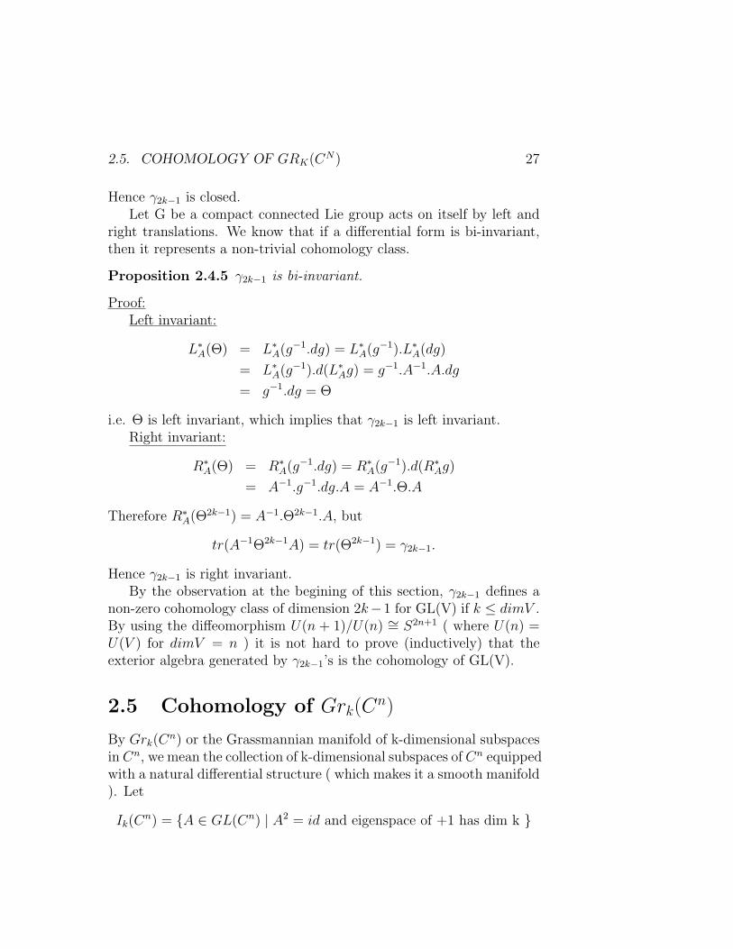
Hence γ2k−1 is closed.Let G be a compact connected Lie group acts on itself by left and
right translations. We know that if a differential form is bi-invariant,then it represents a non-trivial cohomology class.
Proposition 2.4.5 γ2k−1 is bi-invariant.
Proof:Left invariant:
L∗A(Θ) = L∗A(g−1.dg) = L∗A(g−1).L∗A(dg)
= L∗A(g−1).d(L∗Ag) = g−1.A−1.A.dg
= g−1.dg = Θ
i.e. Θ is left invariant, which implies that γ2k−1 is left invariant.Right invariant:
R∗A(Θ) = R∗A(g−1.dg) = R∗A(g−1).d(R∗Ag)
= A−1.g−1.dg.A = A−1.Θ.A
Therefore R∗A(Θ2k−1) = A−1.Θ2k−1.A, but
tr(A−1Θ2k−1A) = tr(Θ2k−1) = γ2k−1.
Hence γ2k−1 is right invariant.By the observation at the begining of this section, γ2k−1 defines a
non-zero cohomology class of dimension 2k−1 for GL(V) if k ≤ dimV .By using the diffeomorphism U(n + 1)/U(n) ∼= S2n+1 ( where U(n) =U(V ) for dimV = n ) it is not hard to prove (inductively) that theexterior algebra generated by γ2k−1’s is the cohomology of GL(V).
2.5 Cohomology of Grk(Cn)
By Grk(Cn) or the Grassmannian manifold of k-dimensional subspaces
in Cn, we mean the collection of k-dimensional subspaces of Cn equippedwith a natural differential structure ( which makes it a smooth manifold). Let
Ik(Cn) = A ∈ GL(Cn) | A2 = id and eigenspace of +1 has dim k

28 Ch 2: VECTOR FIELDS AND LIE DERIVATIVES
Ik(Cn) is a homotopy equivalent to Grk(C
n). Indeed
Ik(Cn) −→ Grk(C
n)
F −→ W
(where W is equal to the +1 eigenspace of F) is a vector bundle withthe fibre over W is
G =
(I b0 −I
)| b ∈ Hom(W ′,W ) where W ⊕W ′ = Cn
Remark: Invk(Cn) = Ik(C
n)∩U(Cn) ∼= Grk(Cn) and this identification
is one way to produce the smooth structure on Grk(Cn). Hence
H∗(Grk(Cn), C) ∼= H∗(Invk(C
n), C).
As before we want to produce closed forms which represent non-trivialcohomology classes. Consider
Invk(Cn)
F→ End(Cn)
A −→ A.
ThenF ∈ Ω0(Invk(C
n), End(Cn))
dF ∈ Ω1(Invk(Cn), End(Cn)).
Definition 2.5.1 σ2r = tr(F (dF )2r) ∈ Ω2r(Invk(Cn), C).
We will prove that σ2r is a closed form.
Lemma 2.5.2 If F is invertible and M ∈ End(Cn),
MF + FM = 0 =⇒ tr(M) = 0.
Proof: tr(MFF−1) = tr(M) = tr(−FMF−1) = −tr(M).
Lemma 2.5.3 If F is an involution (i.e. F 2 = I), then
tr(dF )2r+1 = 0.

2.5. COHOMOLOGY OF GRK(CN) 29
Proof:
F 2 = F.F = I
⇒ dF.F + F.dF = 0
⇒ (dF )2r+1.F + F.(dF )2r+1 = 0
Therefore tr(dF )2r+1 = 0 by the previous lemma.
Proposition 2.5.4 d(σ2r) = 0. i.e. σ2r is closed.
Proof:
d(σ2r) = d(trF (dF )2r) = tr(dF (dF )2r)
= tr(dF )2r+1 = 0.
Since the transitive action of U(Cn) on Grk(Cn) is the action of U(Cn)
on Invk(Cn) by the conjugation, the forms σ2r’s are invariant forms and
it is not hard to see that they represent non-trivial cohomology classes.One way to see that simply notice that they are harmonic. Anotherway to see that consider
U(r + 1)i→ U(k + 1)
j→ U(n)
τ −→ τ =
(τ 00 I
)−→
(τ 00 −I
)which gives
Invr(Cr+1)→ Invk(C
k+1)→ Invk(Cn)
Now it is enough to see that
σ2r |Invr(Cr+1)∈ Ω2r(Invr(Cr+1)) = Ω2r(CP r)
is non-zero.It is possible to prove that
σ2r ∈ H2r( limn→∞
Grk(Cn), C) for r = 1, · · · , k
generate the cohomology. Precisely,
H∗( limn→∞
Grk(Cn)) = Q[σ2, · · · , σ2k],
the polynomial algebra generated by σ2, · · · , σ2k.

30 Ch 2: VECTOR FIELDS AND LIE DERIVATIVES

Chapter 3
S1 - EquivariantCohomologies
3.1 Cohomologies on S1-manifolds
Definition 3.1.1 Let (A∗, d, i) be a differential graded commutative al-gebra with contraction i where d2 = 0 , i2 = 0 and di+ id = 0. Define
PC∗ =
∏A2k if * is even∏A2k+1 if * is odd
D = d+ i
i.e.D(ω0, ω2, · · ·) = (dω0 + iω2, dω2 + iω4, · · ·)
D2 = (d+ i)(d+ i) = d2 + id+ di+ i2 = 0
Definition 3.1.2 C∗+ =∏k≥0A
∗−2k
i.e.Cn
+ = An + An−2 + An−4 + · · ·
(d+ i)(ωn, ωn−2, · · ·) = (dωn, iωn + dωn−2, iωn−2 + dωn−4, · · ·)
C∗− = (∏k≥0
A∗+2k, d+ i)
We also put (C∗, d) = (A∗, d).
31

32 Ch 3: S1 - EQUIVARIANT COHOMOLOGIES
If M is a smooth manifold with an S1−action, let
(A∗, d, i) = (Ω∗inv, d, i)
where iX is the contraction along the vector field defined by the action.
Definition 3.1.3 1. H∗(M) = H∗(C∗).
2. PH∗S1(M) = H∗(PC∗) called periodic cohomology.
3. H∗S1(M) = H∗(C∗+) called equivariant cohomology.
4. GH∗S1(M) = H∗(C∗−) called special equivariant cohomology.
Clearly
C2n+ = Ω2n
inv + Ω2n−2inv + · · ·+ Ω2
inv + Ω0inv
and
C2n−1+ = Ω2n−1
inv + Ω2n−3inv + · · ·+ Ω1
inv.
If for example i = 0 i.e. if the S1-action is trivial, then
1. PH2∗S1(M) =
∏kH
2k(M)
2. PH2∗+1S1 (M) =
∏kH
2k+1(M)
3. H∗S1(M) = H∗(M)⊕H∗−2(M)⊕ · · ·
4. GH∗S1(M) =∏k≥0H
∗+2k(M)
Given (A∗, d, i) as above, we have
(C∗+, D)−2- (C∗+, D) - (C∗, d)
(C∗+, D)−2- (PC∗, D) - (C∗−, D)
∼=
6 6
i
6
When (A∗, d, i) is the one associated to a manifold with an S1-action
3.1. COHOMOLOGIES ON S1-MANIFOLDS 33
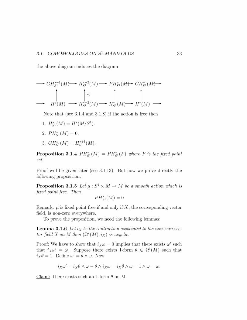
the above diagram induces the diagram
- H∗(M) - H∗−2S1 (M) - H∗S1(M) - H∗(M) -
- GH∗−1S1 (M) - H∗−2
S1 (M) - PH∗S1(M)- GH∗S1(M) -
6 6 6 6∼=
Note that (see 3.1.4 and 3.1.8) if the action is free then
1. H∗S1(M) = H∗(M/S1).
2. PH∗S1(M) = 0.
3. GH∗S1(M) = H∗+1S1 (M).
Proposition 3.1.4 PH∗S1(M) = PH∗S1(F ) where F is the fixed pointset.
Proof will be given later (see 3.1.13). But now we prove directly thefollowing proposition.
Proposition 3.1.5 Let µ : S1 ×M →M be a smooth action which isfixed point free. Then
PH∗S1(M) = 0
Remark: µ is fixed point free if and only if X, the corresponding vectorfield, is non-zero everywhere.
To prove the proposition, we need the following lemmas:
Lemma 3.1.6 Let iX be the contraction associated to the non-zero vec-tor field X on M then (Ω∗(M), iX) is acyclic.
Proof: We have to show that iXω = 0 implies that there exists ω′ suchthat iXω
′ = ω. Suppose there exists 1-form θ ∈ Ω1(M) such thatiXθ = 1. Define ω′ = θ ∧ ω. Now
iXω′ = iXθ ∧ ω − θ ∧ iXω = iXθ ∧ ω = 1 ∧ ω = ω.
Claim: There exists such an 1-form θ on M.

34 Ch 3: S1 - EQUIVARIANT COHOMOLOGIES
Proof of the claim:First consider the case M = Rn and X = ∂
∂xithen θ = dxi. Given M
and x ∈M , letφx : Rn → φx(R
n) = Ux
be a co-ordinate system near x. Given X non-zero, we can choose aco-ordinate system at x in such a way that
(φ−1x )∗(X) =
∂
∂x1
.
Let fx be a partition of unity associated to the cover Ux. Put
θ =∑
fx(φ−1x )∗(dx1)
TheniXθ =
∑fx = 1
Lemma 3.1.7 (Ω∗inv(M), iX) is acyclic when X is a non-zero vectorfield.
Proof: LetA : Ω∗(M)→ Ω∗inv(M)
ω 7→∫S1µ∗t (ω)dt.
A(iXω) =∫S1µ∗t (iXω)
=∫S1iXµ
∗tω
= iX
∫S1µ∗tω
= iX(Aω)
If iXω = 0 then by the previous lemma, there exists ω′ ∈ Ω∗(M) suchthat
iXω′ = ω.
ω′ may not be invariant, but Aω′ ∈ Ω∗inv(M). Now
iXAω′ = AiXω
′ = Aω = ω.

3.1. COHOMOLOGIES ON S1-MANIFOLDS 35
Proof of the proposition (3.1.5): Let ω = (ω0, ω2, · · ·) such that Dω =0. i.e.
dω0 + iXω2 = 0
dω2 + iXω4 = 0
...
We have to choose γ = (γ1, γ3, γ5, · · ·) such that
Dγ = ω.
i.e.iXγ1 = ω0
dγ1 + iXγ3 = ω2
dγ3 + iXγ5 = ω4
...
First by the above lemma, choose γ1 such that iXγ1 = ω0. Now
iX(−dγ1 + ω2) = −iXdγ1 + iXω2
= diXγ1 + iXω2 (because diX + iXd = 0)
= dω0 + iXω2
= 0
therefore there exists γ3 ∈ Ω3inv(M) such that
iXγ3 = −dγ1 + ω2
and hencedγ1 + iXγ3 = ω2.
Similarly given iX(−dγ3 + ω4) = 0 we obtain γ5 as above and also
dγ3 + iXγ5 = ω5.
By repeating the process we obtain γ1, γ3, γ5, · · · and therefore Dω = 0implies that there exists γ such that Dγ = ω.Therefore
PH∗S1(M) = 0.

36 Ch 3: S1 - EQUIVARIANT COHOMOLOGIES
Proposition 3.1.8 If µ : S1 ×M →M is a free action, then
H∗S1(M) ∼= H∗(M/S1).
Proof: Recall that H∗S1(M) = H∗DR(C∗+) where
C2n+ = Ω2n
inv + Ω2n−2inv + · · ·+ Ω2
inv + Ω0inv.
C2n−1+ = Ω2n−1
inv + Ω2n−3inv + · · ·+ Ω3
inv + Ω1inv.
Remark: (1) µ : S1×M →M is a free action implies that Mπ→M/S1
is a submersion.(2) Ω∗(M/S1) ∼= ker iX : Ω∗inv(M)→ Ω∗−1
inv (M).
Lemma 3.1.9 (ker iX , d) → (C∗+, D) induces an isomorphism in thecohomology.
Proof:surjectivity:
Let ω = (ω2n, ω2n−2, · · · , ω2, ω0) represents a cohomology class inC2n
+ .
Dω = 0⇒ dω2n = 0
iXω2n + dω2n−2 = 0...
iXω2 + dω0 = 0
iXω0 = 0
Construct γ = (γ2n−1, γ2n−3, · · · , γ3, γ1) as before. i.e. first choose γ1
such that iXγ1 = ω0 then choose γ3 such that iXγ3 + dγ1 = ω2 and soon.
Nowω −Dγ = (ω2n − dγ2n−1, 0, 0, · · · , 0)
iX(ω2n − dγ2n−1) = iXω2n + diXγ2n−1
= iXω2n + d(ω2n−2 − dγ2n−3)
= iXω2n + dω2n−2
= 0

3.1. COHOMOLOGIES ON S1-MANIFOLDS 37
therefore η = ω −Dγ ∈ ker iX and
η 7−→ ω.
Exercise 3.1.10 Prove the injectivity in the above lemma.
Proposition 3.1.11 Suppose that M is a finite dimensional manifoldand
µ : S1 ×M →M
is a smooth action. Then
PH∗S1(M) = limk→∞
H∗+2kS1 (M).
Proof: Recall thatCn
+ = Ωninv + Ωn−2
inv + · · ·Define
Cn+(k) = Cn+k
+ = Ωn+kinv + Ωn+k+2
inv + · · · .Now C∗+ → PC∗.
(ω2k, ω2k−2, · · · , ω0) 7→ (ω0, ω2, · · · , ω2k, 0, 0, · · · , )
(ω2k−1, ω2k−3, · · · , ω1) 7→ (ω1, ω3, · · · , ω2k−1, 0, 0, · · ·).We can factorize this map as
C∗+S−→ C∗+(2)
S−→ C∗+(4)S−→ · · ·
whereS(ωn, ω2n−2, · · ·) = (0, ωn, ωn−2, · · ·).
ThereforePC∗ = lim
kC∗+(2k).
Hence
PH∗S1(M) = H∗(PC∗)
= H∗(limkC∗+(2k))
= limkH∗(C∗+(2k))
= limkH∗+2kS1 (M).

38 Ch 3: S1 - EQUIVARIANT COHOMOLOGIES
Lemma 3.1.12 Let µM : M × S1 → S1 and µN : N × S1 → S1 besmooth actions and f : M → N be an equivariant smooth map. Iff ∗ : H∗(N)→ H∗(M) is an isomorphism then
f ∗ : H∗S1(N)→ H∗S1(M)
andf ∗ : PH∗S1(N)→ PH∗S1(M)
are also isomorphisms.
Proof: We prove by induction on k where fk : HkS1(N) → Hk
S1(M).First note that
0← Ck ← Ck+
S← Ck+(−2)← 0
(0, ωk−2, ωk−4, · · ·)← (ωk−2, ωk−4, · · ·).
ωk ← (ωk, ωk−2, · · ·)
is a short exact sequnece. Therefore we have the Gysin sequence
· · · ← Hk−1S1 (M)← Hk(M)← Hk
S1(M)← Hk−2S1 (M)← · · ·
By the naturality of Gysin sequence we have the following commu-tative diagram
Hk−1S1 (N) Hk(N) Hk
S1(N) Hk−2S1 (N) Hk−1(N)
Hk−1S1 (M) Hk(M) Hk
S1(M) Hk−2S1 (M) Hk−1(M)
6 6 6 6 6∼= fk−1 ∼= fk fk ∼= fk−2 ∼= fk−1
Therefore five-lemma implies that
fk : HkS1(N)→ Hk
S1(M)
is an isomorphism. Similar proof holds for
fk : PHkS1(N)→ PHk
S1(M).
Proposition 3.1.13 (See 3.1.4) Let µ : S1 ×M → M be a smoothaction and F ⊆M be the fixed point set. Then PH∗S1(M)→ PH∗S1(F )is an isomorphism.
3.1. COHOMOLOGIES ON S1-MANIFOLDS 39
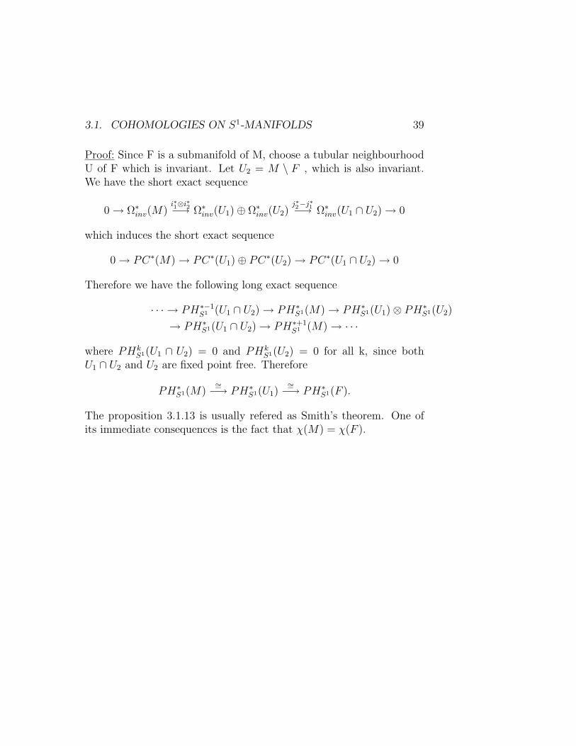
Proof: Since F is a submanifold of M, choose a tubular neighbourhoodU of F which is invariant. Let U2 = M \ F , which is also invariant.We have the short exact sequence
0→ Ω∗inv(M)i∗1⊗i
∗2−→ Ω∗inv(U1)⊕ Ω∗inv(U2)
j∗2−j∗1−→ Ω∗inv(U1 ∩ U2)→ 0
which induces the short exact sequence
0→ PC∗(M)→ PC∗(U1)⊕ PC∗(U2)→ PC∗(U1 ∩ U2)→ 0
Therefore we have the following long exact sequence
· · · → PH∗−1S1 (U1 ∩ U2)→ PH∗S1(M)→ PH∗S1(U1)⊗ PH∗S1(U2)
→ PH∗S1(U1 ∩ U2)→ PH∗+1S1 (M)→ · · ·
where PHkS1(U1 ∩ U2) = 0 and PHk
S1(U2) = 0 for all k, since bothU1 ∩ U2 and U2 are fixed point free. Therefore
PH∗S1(M)∼=−→ PH∗S1(U1)
∼=−→ PH∗S1(F ).
The proposition 3.1.13 is usually refered as Smith’s theorem. One ofits immediate consequences is the fact that χ(M) = χ(F ).

40 Ch 3: S1 - EQUIVARIANT COHOMOLOGIES

Chapter 4
Characteristic Classes andTransfer
4.1 Degree of a map
Let M, N be two smooth oriented manifolds and N also be connected.Let f : M → N be a smooth map such that f is transversal to asubmanifold P of N. Then f−1(P ) is a smooth manifold such that
dimf−1(P ) = dimM − dimN + dimP.
Consider the follwing cases:
1. either f is proper (i.e. the inverse image of every compact set iscompact) and P is compact.
2. or M is compact and P is a closed subset of N.
In the above cases, when p ∈ N is a regular value of f and dim M =dim N = n then,
deg(f) =∑
xi∈f−1(p)
sign(xi)
where
sign(xi) =
+1 if dfxi preserves the orientation−1 otherwise
41

42 Ch 4: CHARACTERISTIC CLASSES AND TRANSFER
Exercise 4.1.1 1. f ∼ g ⇒ deg(f) = deg(g).
2. deg(f g) = deg(f)deg(g).
3. deg(f × g) = deg(f)deg(g).
4. f∗ : Hnc (M)→ Hn
c (N) is the map defined by f∗(1) = deg(f).
4.2 Lefschetz number of a map
Let M be a compact, oriented and smooth manifold. Let f : M → Mbe a smooth map. Let Gf : M → M × M be the graph of f (i.e.f(m) = (m, f(m)) ∈M ×M). Let ∆ be the diagonal of M ×M .
Definition 4.2.1 Choose g ∼ f if needed such that Gg is transversalto ∆. Then the Lefschetz number of f , L(f) is defined by
L(f) =∑
xi∈G−1g (∆)
sign(xi).
Exercise 4.2.2 1. L(f) is independent of g.
2. L(f q g) = L(f) + L(g).
Remark: Lefschetz number is analogous to the trace and if M is notcompact it can be defined only for compact maps where f is compactif f−1(y) is compact for all y.
Definition 4.2.3 The cohomological Lefschetz number of f , LH(f) isdefined by
LH(f) =∑i
(−1)itr(f i).
Proposition 4.2.4 If f has no fixed points then LH(f) = 0.
Exercise 4.2.5 For f : M →M , we have LH(f) = L(f).

4.3. EULER CLASS 43
4.3 Euler class
Let B be an oriented smooth n-manifold. Let Eξ→ B be an oriented
smooth k-vector bundle. Let s0 be the zero section and s : B →E be any section such that s is transversal to s0(B) which may beidentified to B. Then s−1(B) is a smooth manifold of dimension n− kand E(s) = [s−1(B)] = the Poincare dual of s−1(B) ∈ Hk(B). Sinceany two sections are homotopic to each other E(s) is independent of s.
Definition 4.3.1 E(ξ) = the Euler class of ξ = E(s).
Exercise 4.3.2 1. E(ξ1 × ξ2) = E(ξ1)E(ξ2).
2. E(ξ) is natural with respect to pull-backs.
3. L(idB)µ = E(τB) where τB is the tangent bundle of B.
Exercise 4.3.3 If P n1 and P n
2 are oriented closed and cobordant sub-manifolds of Mn+r, then
[P1] = [P2] ∈ Hrc (M).
4.4 Thom’s class
Definition 4.4.1 (Thom’s class) Let ξ : E → B be an oriented realvector bundle where B is an oriented manifold. Let s : B → E be anysection. Then Thom’s class
T (ξ) = [s(B)] ∈ Hncv(E).
Exercise 4.4.2 Verify that this definition coincides with the previousdefinition (See 1.7.5).
Exercise 4.4.3 Verify that the composition
Hncv(E)
i→ Hn(E)
s∗0→ Hn(B)
takes the Thom’s class to the Euler class (where s0 is the zero section).

44 Ch 4: CHARACTERISTIC CLASSES AND TRANSFER
Notice that T (ξ) is characterized by∫ExT (ξ) |Ex= 1
for all x ∈ B. where Ex is the fibre over x.
Exercise 4.4.4 Let π : E → B be a proper surjective smooth mapbetween two smooth manifolds. If π is a submersion, then π : E → Bis a smooth bundle.
Definition 4.4.5 If π : E → B is a proper submersion, then define
Tvert(E) = v ∈ τ(E) | dπ(v) = 0
where τ(E) is the tangent bundle of E.
Proposition 4.4.6 If U ⊆ B is open and F × U → U is the trivialbundle, then
Tvert(F × U) ∼= τ(F )× U.
Exercise 4.4.7 Tvert(E) is orientable ⇒ the fibre F is orientable.
Exercise 4.4.8 Tvert(E) is orientable and B is orientable ⇒ E is ori-entable.
Definition 4.4.9 Let π : E → B be a complex vector bundle. A her-mitian structure <,> is a smoothly varying hermitian scalar producton each fibre.
Properties:
1. Any convex combination of hermitian structures is a hermitianstructure.
2. Any complex vector bundle has a hermitian structure.
3. There is a 1-1 correspondence between the isomorphism classes ofcomplex vector bundles and the isomorphism classes of hermitianvector bundles.

4.5. CHERN CLASSES 45
Let F(B) be the set of all complex line bundles over B and Fh(B)be the set of all complex line bundles over B with hermitian structures.Let F(B)/ ∼ be the isomorphism classes of complex line bundles andFh(B)/ ∼ be the isomporphism classes with hermitian structures. Byproperty (3)
F(B)/ ∼∼= Fh(B)/ ∼
Definition 4.4.10 F(B)/ ∼ has the group structure with the tensorproduct ⊗ as the multiplication. This group is called the Picard groupand denoted by Pic(B).
The trivial line bundle is the identity element. ξ∗ is the inverse of ξbecause,
ξ ⊗ ξ∗ = Hom(ξ, ξ)
id ∈ Hom(ξ, ξ) provides a non-zero cross-section and hence ξ ⊗ ξ∗ istrivial.
Remark: The map
Pic(B) −→ H2DR(B,R)
[ξ] 7−→ E(ξ)
factors through
Pic(B)→ Pic(B)⊗R∼=→ H2
DR(B,R).
Indeed,
Pic(B)⊗R ∼= H2DR(B,R).
4.5 Chern classes
Let π : E → B be a complex vector bundle. We will construct somecohomology classes ci(π) ∈ H2i
DR(B) called the Chern classes with theproperties that
1. ci(π) = 0 for all i > rank π.

46 Ch 4: CHARACTERISTIC CLASSES AND TRANSFER
2. natural with respect to the pull-backs. i.e. if f : B′ → B is asmooth map, then
ci(f∗(E)) = f ∗(ci(π)).
3. c(π1 ⊕ π2) = c(π1)c(π2) where c(π) = 1 + c1(π) + c2(π) + · · ·
4. c1(π) = E(π), the Euler class (if π is a complex line bundle).
Remark: These properties characterizes the Chern classes.Construction of Chern classes:
Definition 4.5.1 Let V be a vector space. The projectivization of V(or the projective space associated to V), denoted by P(V), is definedas the collection of all 1-dimensional subspaces of V; it is a smoothmanifold.
Let Eρ→ B be a complex vector bundle with the transition functions
gαβ : Uα ∩ Uβ → GLn(C).
Definition 4.5.2 The projectivization of a bundle E is the fibre bundle
P (E)φ→ B whose fibre at a point b ∈ B is the projective space P (Eb)
and whose transition functions gαβ : Uα ∩ Uβ → PGLn(C) are induced
by gαβ. (Eb is the fibre over b ∈ B in Eρ→ B).
Consider the following pull-back bundle:
P (E) - M
φ−1(E) - E
? ?
ρ
φ
(∗)
Let
S ′ = (lb, v) ∈ φ−1(E) | v ∈ lb.
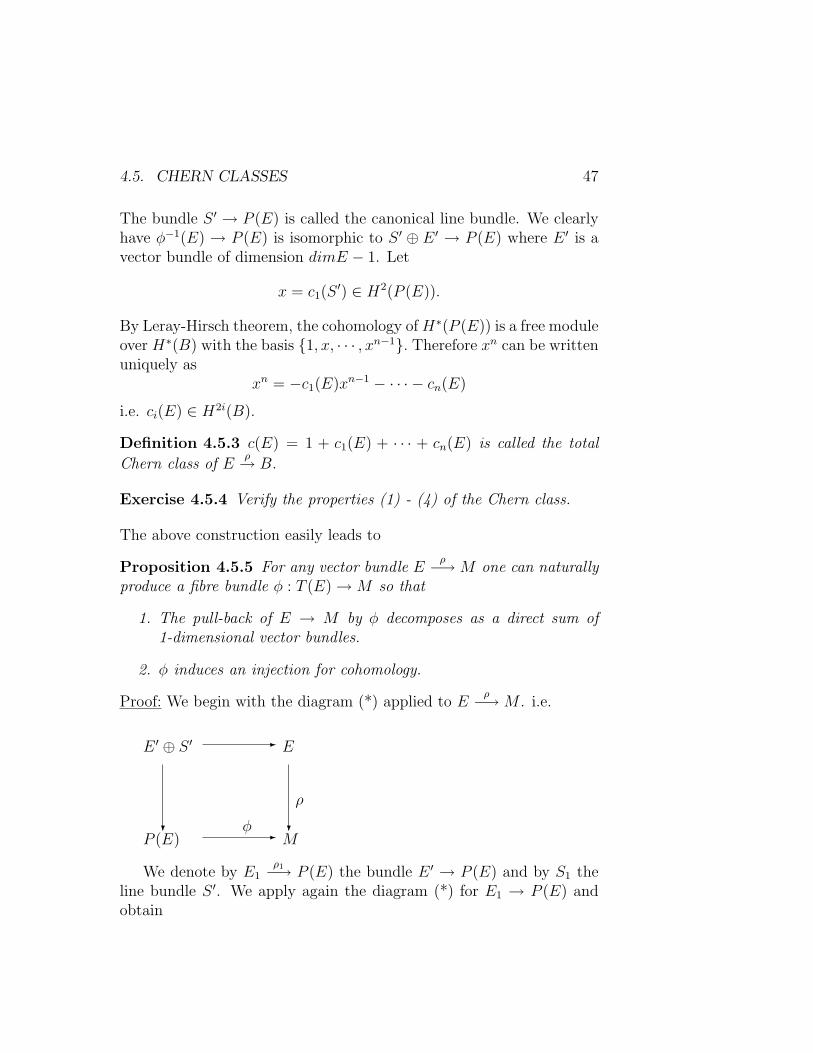
4.5. CHERN CLASSES 47
The bundle S ′ → P (E) is called the canonical line bundle. We clearlyhave φ−1(E) → P (E) is isomorphic to S ′ ⊕ E ′ → P (E) where E ′ is avector bundle of dimension dimE − 1. Let
x = c1(S ′) ∈ H2(P (E)).
By Leray-Hirsch theorem, the cohomology of H∗(P (E)) is a free moduleover H∗(B) with the basis 1, x, · · · , xn−1. Therefore xn can be writtenuniquely as
xn = −c1(E)xn−1 − · · · − cn(E)
i.e. ci(E) ∈ H2i(B).
Definition 4.5.3 c(E) = 1 + c1(E) + · · · + cn(E) is called the total
Chern class of Eρ→ B.
Exercise 4.5.4 Verify the properties (1) - (4) of the Chern class.
The above construction easily leads to
Proposition 4.5.5 For any vector bundle Eρ−→M one can naturally
produce a fibre bundle φ : T (E)→M so that
1. The pull-back of E → M by φ decomposes as a direct sum of1-dimensional vector bundles.
2. φ induces an injection for cohomology.
Proof: We begin with the diagram (*) applied to Eρ−→M . i.e.
P (E) - M
E ′ ⊕ S ′ - E
? ?
ρ
φ
We denote by E1ρ1−→ P (E) the bundle E ′ → P (E) and by S1 the
line bundle S ′. We apply again the diagram (*) for E1 → P (E) andobtain

48 Ch 4: CHARACTERISTIC CLASSES AND TRANSFER
P (E1) - P (E)
E ′1 ⊕ S ′1 - E1
? ?
ρ
φ1
and denote E ′1 = E2 and S ′1 = S2. We continue to denote S1 for thepull-back of S1 → P (E) by φ1, and we get
P (E1) - P (E)
E2 ⊕ S2 ⊕ S1- E1 ⊕ S1
? ?φ1 -
-
M
E
?φ
One continue this construction which will obviously stop after n-steps because dimEi = dimE − i.
The above result is of fundamental importance and is known in theliterature as the ’Spliting principle’. We denote by x1, · · · , xn the Chernclasses of the line bundle S1, · · · , Sn. Obviously xi ∈ H2(T (E)), butbecause of the naturality of the Chern class any symmetric polynomialin x1, · · · , xn interpreted as an element in H∗(T (E)) lies in the imageof H∗(B). Obviously
c1(E) = x1 + · · ·+ xn
c2(E) = x1x2 + · · ·+ xn−1xn...
We will often call x1, · · · , xn as the virtual roots of the characteristicclasses of E.
Definition 4.5.6 Let Eφ→ B be a complex vector bundle. The Chern
character of E, denoted by Ch(E), is defined as
Ch(E) =n∑i=1
exi = n+ (x1 + · · ·+ xn) +1
2(x2
1 + · · ·+ x2n) + · · ·

4.5. CHERN CLASSES 49
i.e. if rankE = n, then
Ch(E) = n+ c1(E) +c1(E)2 − 2c2(E)
2+ · · ·
Also we have
1. Ch(E ⊕ F ) = Ch(E) + Ch(F ).
2. Ch(E ⊗ F ) = Ch(E).Ch(F ).
Definition 4.5.7 Let V be a real vector space. Then the complexifica-tion of V is V ⊗R C.
Let Eξ→ B be a real vector bundle. By complexifying each fibre F to
F ⊗ C we get a complex vector bundle ξC .
Proposition 4.5.8 ξC ∼= ξC, the conjugate bundle.
Proof: Exercise. (Refer Milnor - Characteristic classes.)
Definition 4.5.9 The i-th Pontrjagin classes of ξ is defined by
pi(ξ) = (−1)ic2i(ξC)
i.e.1− p1 + p2 − p3 + · · · = 1 + c2 + c4 + c6 + · · ·
Properties:
1. Pontrjagin classes are natural.
2. p(E ⊗ F ) = p(E).p(F ).
3. p(E ⊕ ε) = p(E) where ε is the trivial bundle.
Examples:
1. p(CP 1) = 1
2. p(CP 2) = 1 + 3u2
3. p(CP 3) = 1 + 4u2
50 Ch 4: CHARACTERISTIC CLASSES AND TRANSFER
4. p(CP 4) = 1 + 5u2 + 10u4
5. p(CP 5) = 1 + 6u2 + 15u4
6. p(CP 6) = 1 + 7u2 + 21u4 + 35u6
where u = −c1(γ1) and γ1 is the canonical line bundle. (Refer Milnorch.classes).
Remark: The homotopy type and the Pontrjagin classes classify 1-connected closed manifolds upto finite ambiguity.
4.6 Transfer in a bundle
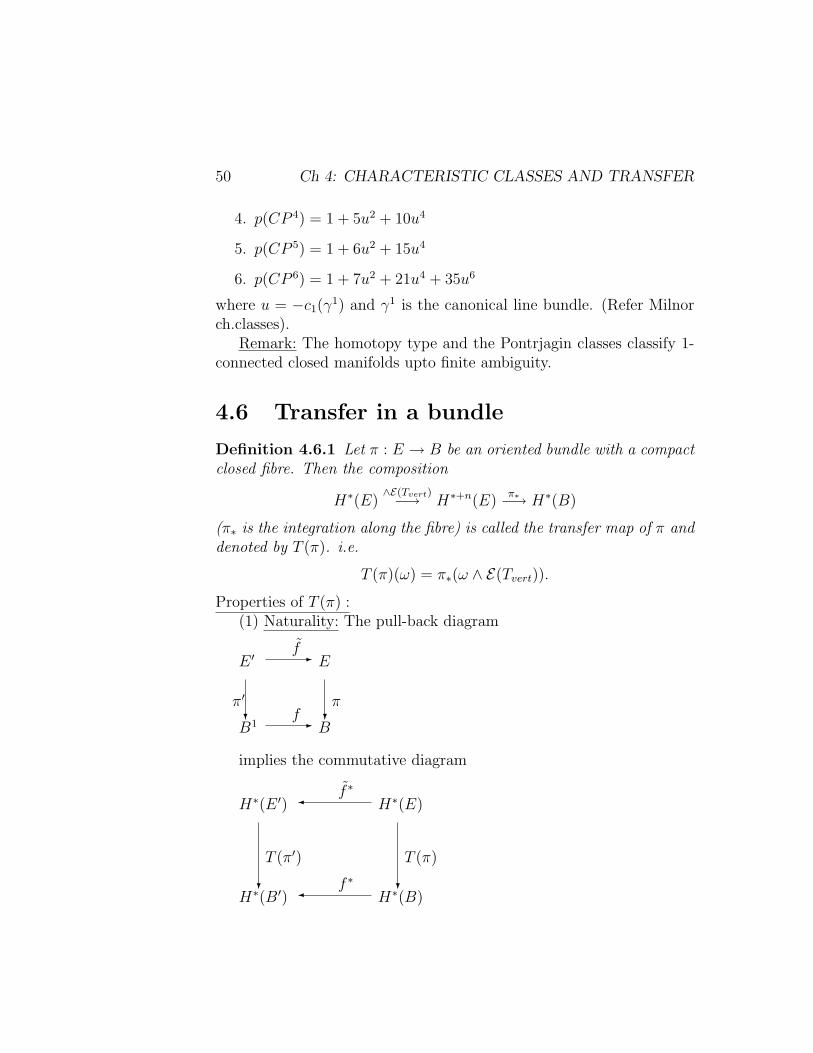
Definition 4.6.1 Let π : E → B be an oriented bundle with a compactclosed fibre. Then the composition
H∗(E)∧E(Tvert)−→ H∗+n(E)
π∗−→ H∗(B)
(π∗ is the integration along the fibre) is called the transfer map of π anddenoted by T (π). i.e.
T (π)(ω) = π∗(ω ∧ E(Tvert)).
Properties of T (π) :(1) Naturality: The pull-back diagram
B1 -f
B
E ′ -f
E
π′? ?
π
implies the commutative diagram
H∗(B′) f ∗
H∗(B)
H∗(E ′) f ∗
H∗(E)
T (π′)
? ?
T (π)

4.6. TRANSFER IN A BUNDLE 51
(2) Functorial: (covariant)i.e. if E1
π1→ E2π2→ B and π = π2 π1 then
T (π2 π1) = T (π2) T (π1).
Proof sketch:
H∗(E1) H∗+n+p(E1) H∗(B)
H∗+n(E1) H∗+p(E2)
H∗(E2)
- -
@@@@R
@
@@@R
@@@@R
?
-
6
λE(Tvπ) π∗
λE(Tvπ1) λπ∗1(E(Tvπ2)) (π1)∗ (π2)∗
(π1)∗ λE(Tvπ2)
T (π1)T (π2)
T (π)
(∗∗)
(In the above diagram Tv means Tvert. Now the proof follows fromthe diagram chasing and from the facts that
(i) the square (∗∗) commutes because of the naturality of the Eulerclass.
(ii) E(Tvertπ) = E(Tvertπ1).π∗1(E(Tvertπ2)).
(iii) Tvertπ = Tvertπ1 ⊕ π∗1(Tvertπ2).
Hence the proof.(3) If B × F π→ B is trivial, then we have
T (π) π∗ = χ(F ).id
Note: (3) ⇒ π∗ is injective if ψ(F ) 6= 0.Proof sketch for (3): Notice that
H∗(B)π∗→ H∗(B × F )
a 7−→ a⊗ 1

52 Ch 4: CHARACTERISTIC CLASSES AND TRANSFER
H∗(B × F ) = H∗(B)⊗H∗(F )ΛE→ H∗+n(B × F )
x⊗ y 7−→ x⊗ E(Tπ)y
(because E(B × τF ) is the pull-back of E(τF ).) Notice also that
π∗(ap ⊗ bq) =
0 if q 6= nap.(bq(θ)) if q = n
(i.e. if q = n, π∗ is the integration with the orientation.)Therefore
H∗(B)→ H∗(B × F )→ H∗(B)⊗H∗(F )→ H∗(B)
a 7−→ a⊗ 1 7−→ a⊗ χ(τF ).1 7−→ a.χ(F )
Theorem 4.6.2 If Eπ→ B is an oriented smooth bundle with ψ(F ) 6=
0, then the composition
H∗(B)π∗−→ H∗(E)
T (π)−→ H∗(B)
is an isomorphism.
4.7 Generalization of Transfer
Let Eπ→ B be a smooth bundle with a compact manifold fiber and let
f : E → E be a smooth map such that π f = π.
Definition 4.7.1 In the above case, we can define T (π, f) : H∗(E)→H∗(B) such that
1. T (π, id) = T (π).
2. if π is trivial (i.e. π : B × F → B is the projection), then
T (π, f) π∗ = L(f).id.

4.7. GENERALIZATION OF TRANSFER 53
3. naturality: Let f : E → E and f ′ : E ′ → E ′. Then the diagram
B′ - B
E ′ - E
π′
6 6
π
α
α
implies the following diagram
H∗(B′) α∗
H∗(B)
H∗(E ′) α∗
H∗(E)
T (π′, f ′)
6 6
T (π, f)
4. functoriality: Let E1π1−→ E2 and E2
π2−→ B be any two bundlesand also π = π2 π1 then
T (π, f) = T (π2) T (π1, f).
Construction: First let us define the generalized Euler class. Let ξ :E
π→ B be a bundle with the zero section s0 : B → E. Let ∆ : E →E ⊕ E be the diagnal map.
Exercise 4.7.2 The pull-back of the normal bundle of ∆(E) in E⊕Eby s0 is the same as the normal bundle of s0(B) in E (which is also thesame as E over B).
Notice that the ordinary Euler class of ξ, E(ξ) can also be defined as
Definition 4.7.3 E(ξ) = s∗0(∆∗[∆(E)] in E ⊕ E)
Definition 4.7.4 Let f : E → E be a smooth map such that π f = π.Then define
E(E, f) = s∗0(∆∗f[∆(E)] in E ⊕ E)

54 Ch 4: CHARACTERISTIC CLASSES AND TRANSFER
where∆f : E → E ⊕ E
e 7→ (e, f(e)).
Definition 4.7.5 The generalized transfer map T (π, f) is the compo-sition
H∗(E)∧E(Tvert(E),f)−→ H∗+n(E)
π∗−→ H∗(B)
Remarks:
1. T (π, f) depends on f only upto fibre preserving homotopy.
2. if f is a compact map ( i.e. f−1(e) is compact ∀e ∈ E) then wecan define the concept of transfer for more general E
π→ B.
Some exercises for the readers.
Exercise 4.7.6 Let G be a compact connected Lie group and H ⊆ G aconnected closed subgroup. Describe in terms of Lie algebras of G andH the de Rham cohomology of G/H.
Exercise 4.7.7 Show that if H ⊇ T where T is a maximal torus of Gthen χ(G/H) 6= 0.
Exercise 4.7.8 Let us suppose that G acts freely on S2n+1. Show thatH∗(S2n+1/G) is concentrated in the even degrees. Show in this casethat the maximal torus of G is S1.
Exercise 4.7.9 Is it possible to produce a map f : CP n → CP n withno fixed points (if n is even)?
Exercise 4.7.10 Calculate the Euler class for the complex Grassman-nian Gk(C
n) equipped with the canonical bundle.
Exercise 4.7.11 Let π : E → B be an oriented vector bundle. Showthat
H∗cv(E) ∼= H∗(E,E \ s0(B)).

Chapter 5
Connection and Curvature
5.1 Introduction
Let us recall various equivalent definitions for the connection.
Definition 5.1.1 Let Eπ→ B be a bundle. Let Γ(E) be the collection
of all sections. A connection in E is given by a map
∇ : Γ(E)→ Ω1(B)⊗Ω0(B) Γ(E)
which satisfies that
∇(f.s) = df ⊗ s+ f∇(s)
for every f ∈ Ω0(B) and s ∈ Γ(E).
Note that Γ(E) is a module in Ω0(B). A reformulation of this definitionis
Definition 5.1.2 A connection is a map
∇ : Ω∗(B)⊗Ω0(B) Γ(E)→ Ω∗(B)⊗Ω0(B) Γ(E)
which satisfies that
1. ∇(1⊗ s) ∈ Ω1(B)⊗Ω0(B) Γ(E) for s ∈ Γ(E).
2. ∇(ω ⊗ s) = dω ⊗ s+ (−1)rω.∇(s) for ω ∈ Ωr(B).
55

56 Ch 5: CONNECTION AND CURVATURE
Exercise 5.1.3 Show that the above two defintions are equivalent.
Lemma 5.1.4 ∇2 is linear. i.e.
∇2(ω ⊗ s) = ω.∇2(s).
Proof:
∇2(ω ⊗ s)= ∇dω ⊗ s+ (−1)rω.∇s= d2ω ⊗ s+ (−1)r+1dω.∇s+ (−1)rdω.∇s+ (−1)2rω.∇2(s)
= ω.∇2(s)
Definition 5.1.5 ∇2 is called the curvature associated to ∇.
Remark: If∇1,∇2 are connections and f, g ∈ Ω0(B) such that f+g = 1,then (f∇1 + g∇2) is a connection.
Proposition 5.1.6 Every bundle has a connection.
Proof:step(1): There exists a connection on a trivial vector bundle. Con-
sider B × Cn → B. In this case,
Γ(E) = Ω0(B)⊗ · · · ⊗ Ω0(B)
i.e. Γ(E) is the directsum of n-copies of Ω0(B). Choose θji ∈ Ω1(B) for1 ≤ i, j ≤ n. Define
∇ : Γ(E)→ Ω1(B)⊗ Γ(E)
as follows:∇(∑i
f isi) =∑i
df i ⊗ si +∑i,j
f iθji ⊗ sj.
Note: If θji = 0 for all i, j then ∇ is called the flat connection.step(2): (for arbitrary bundle).
Let Ui be a trivial open cover such that E |Ui→ Ui is a trivial bun-dle. Let ρi be a partition of unity with respect to Ui. Chooseconnections ∇i for E |Ui→ Ui. Define
∇(s) =∑i
ρi∇i(s |Ei).
5.1. INTRODUCTION 57
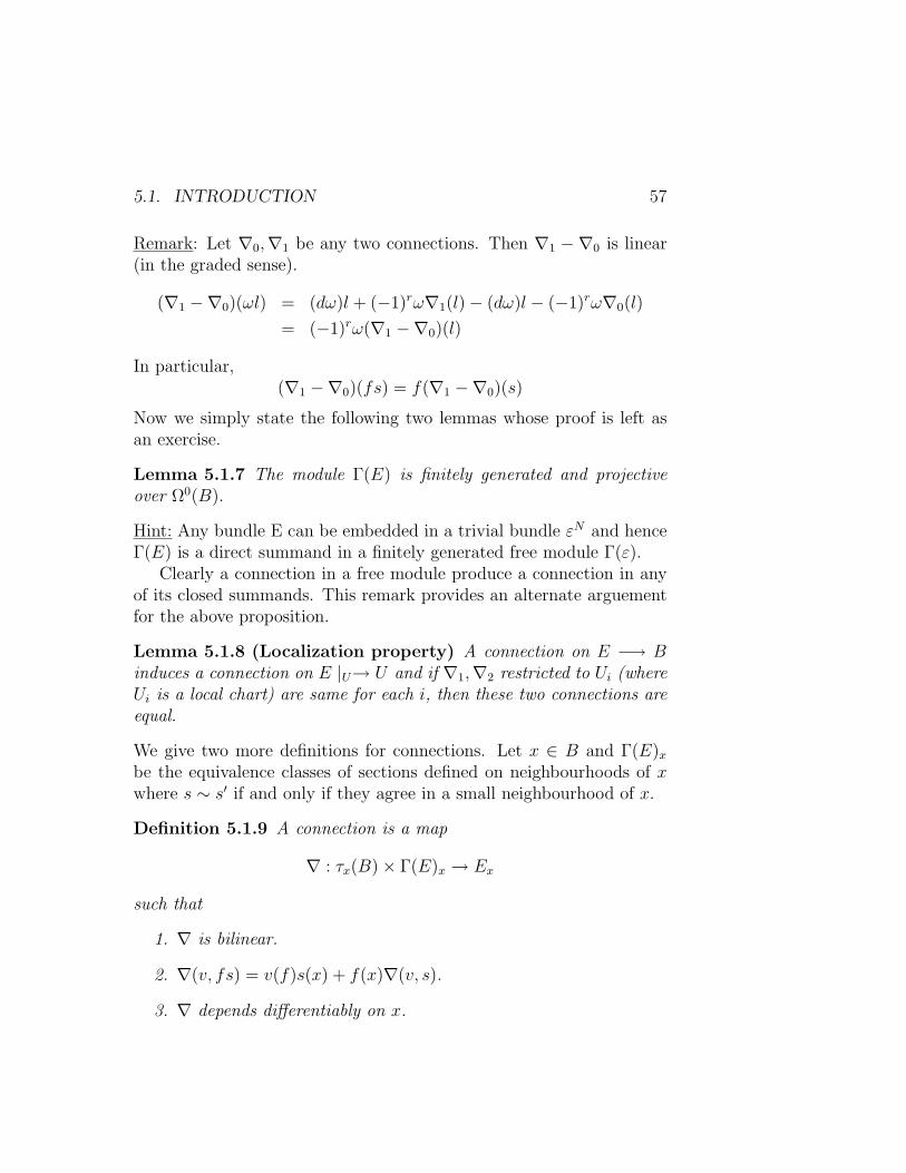
Remark: Let ∇0,∇1 be any two connections. Then ∇1 − ∇0 is linear(in the graded sense).
(∇1 −∇0)(ωl) = (dω)l + (−1)rω∇1(l)− (dω)l − (−1)rω∇0(l)
= (−1)rω(∇1 −∇0)(l)
In particular,(∇1 −∇0)(fs) = f(∇1 −∇0)(s)
Now we simply state the following two lemmas whose proof is left asan exercise.
Lemma 5.1.7 The module Γ(E) is finitely generated and projectiveover Ω0(B).
Hint: Any bundle E can be embedded in a trivial bundle εN and henceΓ(E) is a direct summand in a finitely generated free module Γ(ε).
Clearly a connection in a free module produce a connection in anyof its closed summands. This remark provides an alternate arguementfor the above proposition.
Lemma 5.1.8 (Localization property) A connection on E −→ Binduces a connection on E |U→ U and if ∇1,∇2 restricted to Ui (whereUi is a local chart) are same for each i, then these two connections areequal.
We give two more definitions for connections. Let x ∈ B and Γ(E)xbe the equivalence classes of sections defined on neighbourhoods of xwhere s ∼ s′ if and only if they agree in a small neighbourhood of x.
Definition 5.1.9 A connection is a map
∇ : τx(B)× Γ(E)x → Ex
such that
1. ∇ is bilinear.
2. ∇(v, fs) = v(f)s(x) + f(x)∇(v, s).
3. ∇ depends differentiably on x.

58 Ch 5: CONNECTION AND CURVATURE
This definition is obviously equivalent to
Definition 5.1.10 A connection is a map
∇ : X (B)× Γ(E)→ Γ(E)
such that
1. ∇(fX, s) = f∇(X, s).
2. ∇(X, fs) = X(f)s+ f∇(X, s).
Observations:Ωev(B) ⊗Ω0(B) Γ(E) is a strictly commutative algebra and the cur-
vature restricts to a Ωev(B)-linear map of Ωev(B)⊗ Γ(E) to itself.Consider E = B×Cn → B. Γ(E) is a free module over Ω0(B) with
the basis s1, · · · , sn. Now
∇(s1) =∑
θi1 ⊗ si∇(s2) =
∑θi2 ⊗ si
...
∇(sn) =∑
θin ⊗ si
where θij ∈ Ω1(B). Let R = ∇2 be the curvature. Then
R(sj) = ∇2(sj)
= ∇(θij ⊗ si)= dθij ⊗ si − θij ∧ θki ⊗ sk= dθkj ⊗ sk − θij ∧ θki ⊗ sk= (dθkj − θij ∧ θki )⊗ sk= Rk
j ⊗ sk
Since locally any vector bundle is trivial, the observations above givethe general formulas for connections and curvatures locally.
Let us remember the definitions of trace(T), det(T) and character-istic polynomial for a linear map T : V → V where V is a finitelygenerated projective A-module (A is a commutative ring with unity).

5.2. CHERN-WEIL FORMULA 59
Remark: Let V be a finitely generated projective module over A.Choose V ′ such that V ⊕ V ′ = An. Then T : V → V extends to
T ⊕ 0 : V ⊕ V ′ → V ⊕ V ′.
We define
tr(T ) = tr(T ⊕ 0)
det(T ) = det(T ⊕ idV ′)PT = P(T⊕idV ′ )
where PT = characteristic polynomial of T.It is easy to verify that the above definitions are independent of V ′.
Exercise 5.1.11 If T1 : V1 → V1 and T2 : V2 → V2 are two A-linearmap between finitely generated projective modules, then
∑ 1
k!tr(T1 ⊕ T2)k =
∑ 1
k!tr(T k1 ) +
∑ 1
k!tr(T k2 )
and
∑ 1
k!tr(T1 ⊗ id+ id⊗ T2) =
∑ 1
k!tr(T1)k +
∑ 1
k!tr(T2)k.
5.2 Chern-Weil Formula
Definition 5.2.1 Let Eπ→ B be a vector bundle with a connection ∇.
We have
R∇ : Ωev(B)⊗Ω0(B) Γ(E)→ Ωev(B)⊗Ω0(B) Γ(E).
Define the Chern character
chk(E,∇) =1
k!trace(R
(k)∇ ) ∈ Ωev(B).
Theorem 5.2.2 1. chk(E,∇) ∈ Ω2k(B) and d(chk(E,∇)) = 0.
2. If E is trivial, then chk(E,∇) = dγk for some γk ∈ Ω2k−1(B).

60 Ch 5: CONNECTION AND CURVATURE
3. ch(E) =∑chk(E) = treR where
tr(eR) = tr(id) + tr(R1
1!) + tr(
R2
2!) + · · ·
4. If ∇1,∇2 are connections, then so is ∇1 ⊕∇2. Also
ch(E1 ⊕ E2,∇1 ⊕∇2) = ch(E1,∇1) + ch(E2,∇2).
5. Let E1, E2 → B be two vector bundles with the connections ∇1,∇2.
∇1 : Γ(E1)→ Ω1(B)⊗ Γ(E1)
∇2 : Γ(E2)→ Ω1(B)⊗ Γ(E2)
Γ(E1 ⊗ E2) = Γ(E1)⊗Ω0(B) Γ(E2)
Then∇E1⊗E2 = ∇1 ⊗ id+ id⊗∇2
ch(E1 ⊗ E2,∇E1⊗E2) = ch(E1,∇1) + ch(E2,∇2).
6. If B1f→ B is a smooth map and f ∗(E) → B1 is the pull-back of
E → B by f , then
chk(f∗(E), f ∗(∇)) = f ∗(chk(E,∇))
where
f ∗(∇) : Ω∗(B1)⊗Ω0(B1) Γ(f ∗(E))→ Ω∗(B1)⊗Ω0(B1) Γ(f ∗(E))
is defined as follows:We have the following commutative diagram
Ω∗(B1)⊗Ω0(B) Γ(E) - Ω∗(B1)⊗Ω0(B) Γ(E)
Ω∗(B)⊗Ω0(B) Γ(E) - Ω∗(B)⊗Ω0(B) Γ(E)
f ∗ ⊗ id? ?
f ∗ ⊗ id
∇

5.2. CHERN-WEIL FORMULA 61
claim:
Ω∗(B1)⊗Ω0(B) Γ(E) = Ω∗(B1)⊗Ω0(B1) Γ(f ∗(E)).
proof of the claim:
Ω∗(B1)⊗Ω0(B) Γ(E) = Ω∗(B1)⊗Ω0(B1) Ω0(B1) ⊗Ω0(B) Γ(E)
= Ω∗(B1)⊗Ω0(B1) Ω0(B1)⊗Ω0(B) Γ(E)= Ω∗(B1)⊗Ω0(B1) Γ(f ∗(E))
Therefore we have
f ∗(∇) : Ω∗(B1)⊗Ω0(B1) Γ(f ∗E)→ Ω∗(B1)⊗Ω0(B1) Γ(f ∗E)
proof of the theorem:From the Exercise(5.1.11) (4),(5) and (6) follow immediately.
proof for (1) and (2):When E is trivial, we can choose a base s1, · · · , sn of sections. There-fore ∇ = ‖θji ‖ with θji ∈ Ω1(B). Then the curvature R∇ can bedenoted by the matrix ‖Rj
i‖ where we have already calculated thatRji = dθji − θsi ∧ θjs. Now
chk(E,∇) =1
k!tr(R R · · · R)
=1
k!Ri2i1 ∧R
i3i2 ∧ · · · ∧R
i1ik∈ Ω2k(B)
We need to show that there exists γk such that dγk = chk(E,∇). When
Rji = dθji − θsi ∧ θjs
we have the formula
dRji = θsi ∧Rj
s −Rsi ∧ θjs
called the Bianchi identity.Let 0 ≤ t ≤ 1 be fixed. Then tθji has curvature
Rji (t) = tdθji − t2θsi ∧ θjs

62 Ch 5: CONNECTION AND CURVATURE
LetGk(t) = θi2i1 ∧R
i3i2(t) ∧ · · · ∧Ri1
ik(t).
Define
γk =1
k!k∫ 1
0Gk(t).
We have to verify that dγk = chk(E,∇).Verification: Define
Qk(t) = Ri2i1(t) ∧Ri3
i2(t) ∧ · · · ∧Ri1ik
(t).
Clearly we have
1. k!chk(E,∇) = Qk(1) i.e. t = 1, and
2. Qk(1) =∫ 10
ddt
(Qk(t))
Lemma 5.2.3 dGk(t) = 1k. ddt
(Qk(t)).
Proof: Exercise (Refer: Hicks)Then
dγk =1
k!d(k
∫ 1
0Gk(t))
=1
k!(k∫ 1
0dGk(t))
=1
k!(∫ 1
0
d
dtQk(t))
=1
k!Qk(1)
=1
k!(k!chk(E,∇))
= chk(E,∇).
This proves (2). (1) follows from (2) since locally any bundle is trivialand (1) is a local statement.
Remark: Now chk(E,∇) ∈ Ω2k(B). Let chk(E,∇) ∈ H2k(B) repre-sents its cohomology class.
1. ch(E ⊕ E ′,∇⊕∇′) = ch(E,∇) + ch(E ′,∇′).
5.2. CHERN-WEIL FORMULA 63
2. ch(E,∇) is independent of connections. Therefore we can simplywrite it as ch(E).
Hence we have
ch(E ⊕ F ) = ch(E) + ch(F ).
ch(E ⊗ F ) = ch(E)⊗ ch(F ).
Lemma 5.2.4 If Eπ→ B is a real vector bundle, then
ch2k+1(E,∇) = 0.
The proof will be given below.
Definition 5.2.5 Let Eπ→ B be a complex vector bundle with a her-
mitian structure <,>. We say that a connection ∇ is compatible with<,> if and only if
d < s1, s2 >=< ∇s1, s2 > + < s1,∇s2 > .
1. Each vector bundle has a hermitian structure.
2. There always exists compatible connection with the given hermi-tian structure.
Observation: If the vector bundle is a real bundle then a hermitianstructure is also a Riemannian structure.
Proof of the lemma:It suffices to check the result for a connection compatible with a
Riemannian stucture. In this case, we can prove the more generalresult that
ch2k+1∼= 0.
Since this is a local statement it suffices to check on a small neighbour-hood of points on which the bundle is trivial. For such a neighbourhoodone can choose orthonormal sections s1, · · · , sn ∈ Γ(E) with respect tothe Riemannian metric. Then
θji = −θij

64 Ch 5: CONNECTION AND CURVATURE
and henceRji = −Ri
j.
Therefore the matric R2k+1 is skew symmetric. Hence
ch2k+1(E |U ,∇) ∼= 0.
Note: Instead of 1k!tr(R
(k)∇ ) if we take the coefficient of the characteristic
polynomial of the curvature endomorphism, we would have obtained theusual Chern classes.

Chapter 6
Differential Operators andSymbols
6.1 Differential Operators
Let E → M and F → M be two smooth vector bundles over R or C.Let Γ(E),Γ(F ) be the spaces of smooth sections of the correspondingbundles. Consider the set D : Γ(E) → Γ(F ) | D is a linear map overR or C .
Definition 6.1.1 (Inductively) By definition, the differential opera-tors of order zero are
Diff0(E,F ) = Hom(E,F ).
Then we define the set of differential operators of order k+1 as follows:
Diffk+1(E,F ) = D | [D, f ] ∈ Diffk(E,F ), ∀f ∈ C∞(M)
where [D, f ](s) = D(fs)− fD(s).
Definition 6.1.2 D ∈ Diffk(E,F ) if and only if D : Γ(E) → Γ(F )is linear and for every fi ∈ C∞(M), i = 1, · · · k+1 such that fi(x0) = 0and for every s ∈ Γ(E) we have D(f1f2 · · · fk+1s) = 0 at x0.
It is easy to see that this is equivalent to
65

66 Ch 6: DIFFERENTIAL OPERATORS AND SYMBOLS
Definition 6.1.3 D ∈ Diffk(E,F ) if and only if D : Γ(E) → Γ(F )is linear and for every f ∈ C∞(M) such that f(x0) = 0 and for everys ∈ Γ(E) we have D(fk+1s) = 0 at x0.
Exercise 6.1.4 Show that the last two definitions are equivalent.
Hint:
(k + 1)!a1a2 · · · ak+1 =∑p
∑1≤i1<i2<···<ip≤k+1
(−1)k+p+1(a1 + · · ·+ ap)k+1
Proposition 6.1.5 Definitions 6.1.1 and 6.1.2 (and hence 6.1.3) areequivalent.
Proof: We will prove by induction. Suppose that
Diff(1)i (E,F ) = Diff
(2)i (E,F )
for all i ≤ k. Now
D ∈ Diff (1)k+1(E,F )
⇔ [D, f ] ∈ Diff (1)k (E,F ) = Diff
(2)k (E,F ),∀f ∈ C∞(M).
If f(x0) = 0, then
[D, f ](fk+1s)(x0) = 0
⇒ D(fk+2s)(x0) − f(x0)D(fk+1s)(x0) = 0
⇒ D(fk+2s)(x0) = 0 since f(x0) = 0
⇒ D ∈ Diff (2)k+1(E,F ).
Conversely, let D ∈ Diff(2)k+1(E,F ). Let g ∈ C∞(M) and g =
g − g(x0). Then for any f ∈ C∞(M) such that f(x0) = 0 we have
[D, g](fk+1s)(x0)
= [D, g + g(x0)](fk+1s)(x0)
= D(gfk+1s)(x0) +D(g(x0)fk+1s)(x0)
−(g + g(x0))(x0)D(fk+1s)(x0)
= D(gfk+1s)(x0) + g(x0)D(fk+1s)(x0)
−g(x0)D(fk+1s)(x0)
= D(gfk+1s)(x0)
= 0 since g(x0) = 0
⇒ D ∈ Diff (1)k+1(E,F ).

6.1. DIFFERENTIAL OPERATORS 67
Definition 6.1.6 Diff(E,F ) = ∪∞k=0Diffk(E,F ).
Remark: (a) Diffk(E,F ) ⊆ Diffk+1(E,F ).
(b) The assignment
U ⊆M ; Diffk(E |U , F |U)
is a sheaf. (This is the localization property of the differential opera-tors). i.e. for every U ⊆M , we have a map
ψMU : Diffk(E,F )→ Diffk(E |U , F |U)
such that
1. ψUV .ψMU = ψMV for V ⊆ U ⊆M .
2. if Uα is a cover for M, D1, D2 ∈ Diffk(E,F ) and ψMUα(D1) =ψMUα(D2) for all α then D1 = D2.
3. if Dα ∈ Diffk(E |Uα , F |Uα) and ψUαUα∩Uβ(Dα) = ψUβUα∩Uβ(Dβ) for
all α, β then there exists a unique differential operator D of orderk such that Dα = ψMUα(D) for all α.
4. Let x ∈ U ⊆M and ρ be a smooth function such that the supportof ρ is contained in U with ρ ≡ 1 in a neighbourhood of x in U.Let D be a differential operator of order k. Then
ψMU (D)(s)(x) = D(ρs)(x)
Example: Let U ⊆ Rn be open and E = F = U × C be the trivial
bundles. Let Dk = (−i) ∂∂xk
where i2 = −1. Then
D =∑|α|≤k
Aα1···αn(x)Dα11 · · ·Dαn
n
(with the convention that |α| = ∑αi) is a differential operator of order
k.

68 Ch 6: DIFFERENTIAL OPERATORS AND SYMBOLS
Exercise 6.1.7 Let U be an open subset of Rn. Show that any differ-ential operator of order k from E = U × CN to F = U × CP is of theform
D =∑|α|≤k
Aα1···αn(x)Dα11 · · ·Dαn
n
where Aα1···αn(x) ∈ Hom(CN , CP ) are smooth in x ∈ Rn.
Exercise 6.1.8 If M is compact and D : Γ(E)→ Γ(F ) is a linear mapsuch that the support of D(s) is contained in the support of s for alls ∈ Γ(E) then D is a differential operator of order k.
Hint: Consult R.Narasimhan, Analysis on Real and Complex manifolds,section 3.3.Suppose that the sections s1, · · · , sN locally trivialize E and e1, · · · , ePlocally trivialize F. Let s =
∑f rsr. Then locally
D(s) =∑
(Aα1···αn(x))pr(Dα11 · · ·Dαn
n f r)ep
where Aα1···αn(x) ∈ MPN and Dk = −i ∂
∂xk. This is called the canonical
form. In this case, we simply denote the operator D as
D =∑|α|≤k
Aα(x)Dα.
Example:d : Γ(∧r(T ∗M)) −→ Γ(∧r+1(T ∗M))
is a differential operator of order 1. To find the canonical form considerlocally M = U ⊆ Rn. Then
∧r(T ∗M) = U ×RN
∧r+1(T ∗M) = U ×RP
where N is the cardinality of the set
I = (i1, · · · , ir) | 1 ≤ i1 < · · · < ir ≤ n
and P is the cardinality of the set
J = (j1, · · · , jr+1) | 1 ≤ j1 < · · · < jr+1 ≤ n.

6.2. SYMBOLS 69
Then
d(∑
fi1···irdxi1 · · · dxir)=
∑(√−1(−1)s−1Djsfj1···js···jr+1
)dxj1 · · · dxjr+1
i.e. d =∑nt=1 At(x)Dt where
At(x)JI =
0 if (t, I) 6= J(−1)signσ
√−1 if (t, I) = σ(J)
Exercise 6.1.9 Write down the canonical form for the differential op-erator
d : Ω2(R4)→ Ω3(R4).
Exercise 6.1.10 Let E = Rn×C2 → Rn be the trivial complex vectorbundle of rank 2 and θji =
∑nr=1 ω
j,ri (x)dxr for 1 ≤ i, j ≤ 2 be a matrix
of 1-form, where ωj,ri (x) ∈ Ω0(Rn). Consider the connection ∇ givenby ‖θji ‖ as a differential operator
∇ : Γ(E)→ Ω1(Rn)⊗ Γ(E)
Write down ∇ as a differential operator in the canonical form.
6.2 Symbols
Let V be a finite dimensional complex vector space and Polyk(V ) bethe set of all polynomials of degree atmost k with complex coefficients.Let Polyp(V ) be the set of all homogeneous polynomials of degree pwith complex coefficients. Then
Polyk(V ) = ⊗kp=0Polyp(V ).
If we apply the functor Polyk ( fiberwise ) to the complex vector bundleE → M , we get a complex vector bundle Polyk(E)→ M. Let E,F →M be two complex vector bundles. Then we have the bundle
Polyk(T∗M)⊗Hom(E,F )→M.
Sections of this bundle are locally matrices with polynomial coefficientsor in another description, polynomials with coefficients as linear trans-formations.

70 Ch 6: DIFFERENTIAL OPERATORS AND SYMBOLS
Definition 6.2.1 Symbols are defined as
Symbk(E,F ) = Γ(Polyk(T∗M)⊗Hom(E,F )).
Theorem 6.2.2 There exists a linear map
σ : Diffk(E,F )→ Symbk(E,F )
called principal symbol such that
0→ Diffk−1(E,F )→ Diffk(E,F )σ→ Symbk(E,F )
is exact.
Definition of σ :Let D ∈ Diffk(E,F ). We want
σ(D) ∈ Symbk(E,F ) = Γ(Polyk(T∗M)⊗Hom(E,F )).
i.e. for x ∈M ,
σ(D)(x) ∈ Polyk(T ∗x (M)⊗Hom(Ex, Fx)).
Let ξ ∈ T ∗xM and s ∈ Ex. Choose s ∈ Γ(E) such that s(x) = s andchoose f ∈ C∞(M) such that f(x) = 0 and dfx = ξ. Then define
σ(D)(x)(ξ)(s) =
√−1
k
k!D(fks)(x) ∈ Fx.
We will leave it as an exercise to verify that the above definition isindependent of the choices of f and s.
Locally, let E = U × CN and F = U × CP where U is open in Rn.Let D =
∑|α|≤k Aα(x)Dα. If ξ =
∑ξjdxj, then
dfx =∑ ∂f
∂xjdxj =
∑ξjdxj
⇒ ∂f
∂xj= ξj for all j
⇒ Djf =√−1ξj.

6.2. SYMBOLS 71
Therefore
σ(D)(x)(ξ)(s)
=
√−1
k
k!
∑|α|≤k
Aα(x)Dα11 · · ·Dαn
n (fks)(x)
=
√−1
k
k!
∑|α|=k
Aα(x)Dα11 · · ·Dαn
n (fks)(x)
since the derivatives of order less than k will have
the factor f(x) = 0, they all vanish.
=∑|α|=k
Aα(x)(∂f
∂x1
)α1 · · · ( ∂f∂xn
)αn(s)
=∑|α|=k
Aα(x)ξα11 · · · ξαnn (s).
Thereforeσ(D)(x)(ξ) =
∑|α|=k
Aα(x)ξα11 · · · ξαnn .
To prove the exactness of the theorem it is enough to prove in the trivialcase, since all the three terms satisfy the localization property. But bythe above local representation, it is clear that
Kerσ = Diffk−1(E,F ).
Let E,F →M be two hermitian vector bundles. Let ω ∈ Ω(M) bea non-vanishing top degree form. Let s, t ∈ Γ(E). Then
s, t=∫M< s, t >x ω
is a scalar product. Now one has the construction of formal adjoint *
Diffk(E,F )→ Diffk(F,E)
such that Ds, t= s,D∗t
for compactly supported s ∈ Γ(E) and t ∈ Γ(F ).

72 Ch 6: DIFFERENTIAL OPERATORS AND SYMBOLS
Uniqueness: Adjoint is unique, because D∗1 and D∗2 are the adjointsof D implies that ∫
M< s, (D∗1 −D∗2)(t) >= 0.
Existence: Because of the uniqueness of D∗, it suffices to prove theexistence of D∗ locally. Locally if D corresponds to A(x) then D∗
corresponds to A(x).i.e. when k = 0,If D(f rsr) = Aα(x)prf
rep, then
D∗ = Aα(x)
when k = 1Let D =
∑Aα(x)Dα1
1 · · ·Dαkk where Dj = −
√−1 ∂
∂xjand |α| = 1.
i.e.
D
f 1
...fn
=∑
Aα(x)
Dαf 1
...Dαfn
where (f 1, · · · , fn) = s.
In particular, for example, let α = (1, 0, · · · , 0) then D = D1 where
D1
f 1
...fn
= I
D(1,0,···,0)f 1
...D(1,0,···,0)fn
Then we will have
D∗1 = D1 −D1ω
ωI
where ω = ωdx1 · · · dxn.Generally, if D =
∑|α|≤k Aα(x)Dα1
1 · · ·Dαnn then
D∗ =∑|α|≤k
(Dαnn )∗ · · · (Dα1
1 )∗A∗α(x).
i.e. if D = Aα(x)Dα then
D∗ =∑
(Dα)∗A∗α(x)
Exercise 6.2.3 1. (D1 D2)∗ = D∗2 D∗1.
2. σ(D∗, x) = σ(D, x)∗.

6.3. ELLIPTIC DIFFERENTIAL OPERATORS 73
6.3 Elliptic differential Operators
Definition 6.3.1 Let D : Γ(E) → Γ(F ) be a differential operator oforder k. D is called elliptic if for every x ∈M, ξ( 6= 0) ∈ T ∗xM ,
σ(D)(x)(ξ) : Ex → Fx
is injective.
Remark: Locally, E = U × CN , F = U × CP and D =∑Aα(x)Dα.
Also
σ(D)(x) : T ∗xM → Hom(CN , CP )
ξ 7−→∑|α|=k
Aα(x)ξα.
Then D is called elliptic if for every x and for every non-zero ξ thelinear map
∑|α|=k Aα(x)ξα is injective.
Example: Consider a connection
∇ : Γ(E)→ Γ(T ∗M ⊗ E) = Ω1(M)⊗Ω0(M) Γ(E)
defined by
∇(f rsr) = df r ⊗ sr + f rθpr ⊗ spwhere θpr ∈ Ω1(M). If v =
∑λrsr, choose f such that f(x) = 0 and
dfx = ξ. Then (at x)
σ(∇, x)(ξ)(v)
= σ(∇, x)(ξ)(∑
λrsr)
=√−1∇(
∑fλrsr)
=√−1[
∑d(fλr)⊗ sr+
∑fλrθpr ⊗ sp]
=√−1
∑λrdfx ⊗ sr since f(x) = 0
=√−1ξ ⊗
∑λrsr
=√−1ξ ⊗ v
i.e. connections are elliptic operators of order 1.
74 Ch 6: DIFFERENTIAL OPERATORS AND SYMBOLS
Definition 6.3.2 Let E1, E2, · · · , En −→ M be n vector bundles. LetDi : Γ(Ei) → Γ(Ei+1) be differential operators of order k and supposethat Di+1 Di = 0. Then the sequence Di : Γ(Ei)→ Γ(Ei+1) is calledan elliptic complex if it is exact at the symbol level for all ξ ∈ T ∗M\0.i.e. for any x and ξ,
0→ (E1)xσ(D1)x−→ (E2)x → · · · → (En)x → 0
is exact.
Definition 6.3.3 Let M be a compact manifold and di be an ellipticcomplex operator with
dimKerdi/Imdi−1 = βi <∞
Then the analytical index of the complex di can be defined as
Index(di) =∑
(−1)iβi.
Example: The de Rham complex
d : Ωi(M)⊗ C → Ωi+1(M)⊗ C
is the simplest example for elliptic complex. To see this, first one shouldshow that
σ(d, x)(ξ) : Λi(T ∗xM)→ Λi+1(T ∗xM)
ω 7−→√−1ξ ∧ ω.
By using this fact, one can prove that the symbol sequence is exact (formore detail refer Gilkey p40).
Definition 6.3.4 Let M be compact and D : Γ(E) → Γ(F ) be anelliptic operator of order k and dim(E) = dim(F ). Then
Index(D) = dim(KerD)− dim(CokerD)
= dim(KerD)− dim(KerD∗).
Note: D elliptic ⇒ D∗ elliptic.

Chapter 7
K-Theory
7.1 Definition of K(X)
Definition 7.1.1 Two vector bundles E1, E2 → X are called concor-dant if there exists a vector bundle
E → X × [0, 1]
such that E |X×0∼= E1 and E |X×1∼= E2.
Remarks:
1. If X is paracompact then E1, E2 concordant ⇒ E1∼= E2.
2. If E is a vector bundle over a finite dimensional paracompactspace X, then there exists F such that E ⊕ F is trivial.
In the following discussion we will consider the pair (X, Y ) where Xis paracompact, locally compact and finite dimensional space, Y ⊆ Xis open and there exists a closed set K such that K is a deformationretract of Y. Example, X = Rn, Y = Rn \ 0 and K = Sn−1.
Define the contravariant functor
K : Top −→ Commutative rings.
as follows:Let C(X) be the concordance classes of pairs (ξ, η) of the vector
bundles over X. Then C(X) is a commutative semi-ring with the oper-ations
75

76 Ch 7: K-THEORY
1. (ξ1, η1) + (ξ2, η2) = (ξ1 ⊕ ξ2, η1 ⊕ η2).
2. (ξ1, η1).(ξ2, η2) = ((ξ1 ⊗ ξ2)⊕ (η1 ⊗ η2), (ξ1 ⊗ η2)⊕ (ξ2 ⊗ η1)).
C(X) has the zero element (0, 0). Now define
C0(X) = (ξ, η) ∈ C(X) | ξ ⊕ θ ∼= η ⊕ θ for some θ
C0(X) is an ideal.
Definition 7.1.2 K(X) = C(X)/C0(X).
Note: K(X) is a commutative ring with the unity and K is a contravari-ant functor.
7.2 Definition of K(X,Y)
We can also define the relative K-theory for the topological pairs suchthat K(X,φ) = K(X) and K(X, Y )→ K(X)→ K(Y ) is exact.
Let (ξ, η, φ) denote a pair of vector bundles over X such that ξ |Yφ−→
η |Y is an isomorphism. Define an equivalence relation ∼ (concor-dance) by (ξ1, η1, φ1) ∼ (ξ2, η2, φ2) if there exists a pair of vector bun-dles (ξ, η, φ) over X × I (i.e. φ : ξ |Y×I→ η |Y×I is an isomorphism)such that
1. (ξ, η, φ) |X×0∼= (ξ1, η1, φ1).
2. (ξ, η, φ) |X×1∼= (ξ2, η2, φ2).
Let C(X, Y ) be the concordance classes of pairs of bundles under theabove equivalence relation. We can define the operations on C(X, Y )as
(ξ1, η1, φ1) + (ξ2, η2, φ2) = (ξ1 ⊕ ξ2, η1 ⊕ η2, φ1 ⊕ φ2).
C(X,Y) is a commutative semi-group.
C0(X, Y ) = (ξ, η, φ) ∈ C(X, Y ) | there exists a vector bundle θ
over X, and an isomorphism λ : ξ ⊕ θ → η ⊕ θ such
that the restriction λ : ξ ⊕ θ |Y→ η ⊕ θ |Y is φ⊕ id.
Obviously C0(X, Y ) is a subgroup.

7.2. DEFINITION OF K(X,Y) 77
Definition 7.2.1 (a) K(X, Y ) = C(X, Y )/C0(X, Y ).
Lemma 7.2.2 K(X, Y ) is an abelian group.
Proof: Additive inverse of (ξ, η, φ) = (η, ξ, φ−1). For,
(ξ, η, φ) + (η, ξ, φ−1) = (ξ ⊕ η, η ⊕ ξ, φ⊕ φ−1) ∼ (ε, ε, id)
Note that (A 00 A−1
)joins to (
I 00 I
)canonically by(
A 00 I
)(costI sintI−sintI costI
)(A−1 00 I
)(costI −sintIsintI costI
)
(K(X, Y ) is even a commutative ring, but the next definition, whichwe define shortly is better suited to describe the multiplication).
Example:Let E,F → X be two vector bundles over X. Let D : Γ(E)→ Γ(F )
be an elliptic differential operator of order k and suppose that rankE =rankF . Then we can think of σ(D) as an element of K(T ∗M,T ∗M \0) as explained below:
Now for x ∈M,ω ∈ T ∗xM we have that
σ(D, x)(ω) ∈ Hom(Ex, Fx)
is an isomorphism. Also (π∗E)ω ∼= Ex and (π∗F )ω ∼= Fx. Therefore
σ(D, x)(ω) ∈ Hom((π∗E)ω, (π∗F )ω).
Hence
(π∗E, π∗F, σ(D) |T ∗M\0) ∈ K(T ∗M,T ∗M \ 0).

78 Ch 7: K-THEORY
Definition 7.2.3 An admissible system of vector bundles is a systemof vector bundles ξ1, ξ2, · · · ξn −→ X with αi : ξi |Y→ ξi+1 |Y such that
0 −→ ξ1 |Yα1−→ ξ2 |Y
α2−→ · · · −→ ξn |Y−→ 0
is exact.
As before, let C(X, Y ) be the concordance classes of all admissiblesystems. Let
C0(X, Y ) = ImC(X,X)→ C(X, Y ).The map C(X,X)→ C(X, Y ) is not injective.
Definition 7.2.4 (b) K(X, Y ) = C(X, Y )/C0(X, Y ).
Proposition 7.2.5 K(X, Y ) in the above definition is a group.
Proof: Exercise.
Lemma 7.2.6 The two definitions of K(X, Y ) are equivalent.
Proof: There exists a clear homomorphism
Ka(X, Y ) −→ Kb(X, Y )
defined by
(ξ, η, φ) 7→ (E0, E1, α0) = (E(ξ), E(η), φ).
We needKb(X, Y ) −→ Ka(X, Y ).
First consider the exact sequence of hermitian vector spaces
0 −→ V0α0−→ V1
α1−→ · · · −→ V2n −→ 0
Then[α] : ⊕ni=0V2i −→ ⊕ni=1V2i−1
is an isomorphism where
[α](x0, x2, · · · , x2n) = (α0(x0) + α∗1(x2), α2(x2) + α∗3(x4), · · ·).Now for any given (E0, E1, · · · , En, α0, α1, · · · , αn−1) pick hermitian struc-ture on each Ei and let E = ⊕E2i and F = ⊕E2i−1 and then fiberwisechoose α as in the above vector space case. Then we have
(E,F, α) ∈ Kb(X, Y ).

Chapter 8
Index of DifferentialOperators
8.1 Basic Definitions
Let M be a compact manifold and let E,F → M be any two complexvector bundles. Let Ellk(E,F ) be the set all elliptic operators of or-der k. D ∈ Ellk(E,F ) gives σ(D) ∈ K(T ∗M,T ∗M \ 0) where 0denote the image of the zero section. In this section H∗(X, Y ) meanseither H∗(X, Y ;Q) or H∗(X, Y ;C). Our aim is to define a map, calledTopological index,
Ind : K(T ∗M,T ∗M \ 0) −→ Q (actually in Z)
For his purpose, we need the following:The Chern character
Ch : K(X, Y )→ Hev(X, Y )
and the Todd class
Td : V ect(X)→ Hev(X)
where Vect(X) is the set of all complex vector bundles over X (moduloconcordence).
Given a complex vector bundles E(ξ) over X of rank n, let xi’s bethe virtual roots of E (by the splitting principle). Recall the followingdefinition from Chapter 4.
79
80 Ch 8: INDEX OF DIFFERENTIAL OPERATORS
Definition 8.1.1
c(ξ) =n∏i=1
(1 + xi) = 1 + c1 + · · ·+ cn
ch(ξ) =n∑i=1
exi
= n+ (x1 + x2 + · · ·+ xn) +(x2
1 + · · ·+ x2n)
2+ · · ·
= n+ c1(ξ) +c2(ξ)− 2c1(ξ)2
2+ · · ·
Td(ξ) =n∏i=1
xi1− e−xi
= 1 +c1
2+c2 + c2
1
12+ · · ·
Exercise 8.1.2 Let M = Mg be the oriented surface of genus g andτM be the tangent bundle of M. Then
1. E(τM) = (2− 2g)u
2. c(τM) = 1 + (2− 2g)u
3. ch(τM) = 1 + (2− 2g)u
4. Td(τM) = 1 + (1− g)u
where u is the fundamental class given by the orientation.
Exercise 8.1.3 Let M = CP 2 then τM ⊕ ε = ξ∗ ⊕ ξ∗ ⊕ ξ∗
1. c(τM) = (1 + u)3 = 1 + 3u+ 3u2
2. ch(τM) = 3eu − 1 = 2 + 3u+ 32u2
3. Td(τM) = 1 + 32u+ u2
where u ∈ H2(CP 2;C) represents the generator of the cohomology ofCP 2.
The Chern character ch gives a well-defined ring homomorphism, alsodenoted by ch
K(X)ch−→ Hev(X)

8.1. BASIC DEFINITIONS 81
[ξ, η] 7−→ ch(ξ)− ch(η)
which in turn induces the map (for a pair of “nice” spaces)
ch : K(X, Y ) −→ Hev(X, Y )
as follows:case(1) when Y = * We have the following commutative diagram
Hev(X, ∗) - Hev(X) - Hev(∗) - 0
0 - K(X, ∗) - K(X) - K(∗) - 0
? ? ?
Since the surjective map Hev(X) → Hev(∗) splits, the above commu-tative diagram provides the required map ch : K(X, ∗)→ Hev(X, ∗).
case(2) When Y is a closed subspaces of X and the pair (X,Y) are’good’ spaces (say ANR’s)
In this case the required map is constructed through the followingcommutative diagram
K(X,A) −−−− >Hev(X,A)
K(X/A, ∗) - Hev(X/A, ∗)
∼=
6 6
∼=
case(3) When (X,Y) has (X,A) as a deformation retract as in case(2)This case follows from the following commutative diagram
K(X, Y ) −−−− >Hev(X, Y )
K(X,A) - Hev(X,A)
∼=
6 6
∼=

82 Ch 8: INDEX OF DIFFERENTIAL OPERATORS
For example, when X = T ∗M,Y = T ∗M \ 0 and A = T ∗M \D(0) we have the map
ch : K(T ∗, T ∗M \ 0) −→ Hev(T ∗M,T ∗M \ 0).
Definition 8.1.4 If M is a closed smooth manifold, the (topological)index is defined as the following group homomorphism
Ind : K(T ∗M,T ∗M \ 0) −→ Q (actually in Z)
σ −→ (−1)n[ch(σ).π∗Td(τM ⊗ C)][T ∗M ]
where [T ∗M ] is the fundamental class.
Note thatch(σ) ∈ Hev(T ∗M,T ∗M \ 0)
andπ∗Td(τM ⊗ C) ∈ Hev(T ∗M,T ∗M \ 0).
Recall that if M is oriented, we have the Thom isomorphism π∗
H∗(M)π∗←− H∗+nc (T ∗M) = H∗+n(T ∗M,T ∗M \ 0).
Proposition 8.1.5 If M is oriented, then
Ind(σ) = (−1)n(n+1)
2 [π∗(ch(σ)).Td(τM ⊗ C)][M ].
Proof: Let π : E → M be an oriented vector bundle; a ∈ Ω∗(E) withthe compact support on each fibre and b ∈ Ω∗(M). Then we have theprojection formula ( refer for example, Bott-Tu p63)
π∗(aπ∗(b)) = π∗(a)b
Therefore when E = T ∗M ,
(−1)n[aπ∗(b)][T ∗M ] = (−1)n∫T ∗M
aπ∗(b)
= (−1)n(n+1)
2
∫M
∫Vaπ∗(b)
= (−1)n(n+1)
2
∫Mπ∗(aπ
∗(b))
= (−1)n(n+1)
2
∫Mπ∗(a)b
= (−1)n(n+1)
2 [π∗(a)b][M ].
Now take a = ch(σ) and b = Td(τM ⊗ C).

8.2. INDEX ON TRIVIAL BUNDLES 83
Proposition 8.1.6 If M is an odd dimensional closed smooth mani-fold, then
Ind(σ(D)) = 0.
Proof: Let α : T ∗M → T ∗M be the convolution ξ → −ξ, which induces
α∗ : K(T ∗M,T ∗M \ 0)→ K(T ∗M,T ∗M \ 0).
Notice that
α∗(E,F, σ(D)(x, ξ)) = (α∗E,α∗F, σ(D)(x,−ξ))= (E,F, σ(D)(x,−ξ)).
Since a matrix A is homotopic to −A through the matrices eiπtA weget,
ind(σ) = Ind(α∗(σ)).
ButInd(α∗(σ)) = (−1)nInd(σ).
Therefore if n is odd, then Ind(σ) = 0.Remark: In fact, if the dimension of M is odd then Ind(σ) = 0 for
any σ ∈ K(T ∗M,T ∗M\0), not necessarily the symbol of a differentialoperator.
8.2 Index on Trivial Bundles
Let M be a compact manifold. Consider the trivial vector bundlesE = F = M × CN over M. Let D ∈ Ellk(E,F ). Since Ex and Fx arecanonically isomorphic to CN ,
σ(D)(ξ)(x) : CN → CN
i.e. for each x,
σ(D)(x) : T ∗M \ 0 → GLN(C)
which gives an element in K(T ∗M,T ∗M \ 0). Therefore we have amap
[SM,GLN(C)] ' [T ∗M \ 0, GLN(C)] −→ K(T ∗M,T ∗M \ 0)
84 Ch 8: INDEX OF DIFFERENTIAL OPERATORS
where SM is the sphere bundle associated to the cotangent bundle.Next we want to define the map ch explicitely and verify the fol-
lowing commutative diagram.
Hodd(SM) ' Hodd(T ∗M \ 0) -δHev(T ∗M,T ∗M \ 0)
[SM,GLN(C)] ' [T ∗M \ 0, GLN(C)] - K(T ∗M,T ∗M \ 0)
ch
? ?
ch
More generally, we define a map
[X,GLN(C)]ch−→ Hodd(X;Q)
for any manifold X as follows:
ch(f) =N∑k=1
(−1)k−1
(k − 1)!f ∗hNk
where hNk ∈ H2k−1(GLN ;Q) is described below:Description of hNk :Let UN ⊆ GLN(C) be the unitary group.
S2N−1 ← UN ← UN−1
is a fibration with fibre S2N−1. Define
hNN ∈ H2N−1(UN) = H2N−1(GLN)
as the pull-back of the fundamental class of S2N−1.For ∗ ≤ 2N − 3, H∗(UN−1) = H∗(UN) and hence define
hNN−1 = hN−1N−1 ∈ H2N−3(UN−1).
By induction one can now define hNN−2, · · · , hN1 . We leave the commu-tativity as an exercise.
From the above discussion, we have the following proposition:

8.3. INDEX OF THE DE RHAM OPERATOR 85
Proposition 8.2.1 If E,F are trivial bundles of rank N over a compactclosed manifold M of dimension n, then
Ind(σ) = (−1)n[N∑i=1
(−1)i−1
(i− 1)!σ∗(hNi )π∗(Td(τM ⊗ C))][SM ].
Remark: Suppose that M is stably parallelizable. i.e. τ(M)⊕εN ∼= εN+n
for some N. Then
Td(τM ⊗ C) = Td(ε) = 1.
Exercise 8.2.2 If Mn is a closed compact manifold of dimension nembedded in Rn+1, then M is stably parallelizable.
Remark: Suppose that M is stably parallelizable, then
Ind(σ) =(−1)2n−1
(n− 1)![σ∗(hn)][SM ].
This index is equal to the topological degree of the composition
(SM)2n−1 −− > Un → S2n−1
Note: (SM)2n−1 → UN factors uniquely upto homotopy
(SM)2n−1 −− > Un → UN
since the spaces Un and UN have the same homotopy type upto dimen-sion 2n− 1.
8.3 Index of the de Rham Operator
Theorem 8.3.1 Let Mn (n=2l) be a compact oriented smooth mani-fold. We know that di : Ωi(M) → Ωi+1(M) is an elliptic complex.Then Ind(σdi) = χ(M), the Euler characteristic of M.
Proof: Recall that
Ind(σ) = (−1)n(n+1)
2 [π∗(ch(σ))Td(τM ⊗ C)][M ]

86 Ch 8: INDEX OF DIFFERENTIAL OPERATORS
where π∗ is the Thom isomorphism. The result follows once we checkthat
(−1)n(n+1)
2 [π∗(ch(σ))Td(τM ⊗ C)] = E
where E is the Euler class of τM .Let ξ : E
π−→ BSO(2n) be the universal 2n-dimensional orientedvector bundle and σ′ ∈ K(E,E \ 0) be the element in the complexK-theory defined by the sequence of vector bundles
· · · ,Λiπ∗(EC),Λi+1π∗(EC), · · ·
(where EC → BSO(2n) is the complex vector bundle ξ ⊗ C) and thesequence of bundle map
σ′i : Λiπ∗(EC) |E\0−→ Λi+1π∗(EC) |E\0
defined in the fibre over v ∈ E \0 by the exterior multiplication withv. Precisely
(Λiπ∗(EC))v = Λi(Eπ(v) ⊗ C)
andσ′i(v) = ∧v ⊗ 1.
Let M → BSO(2n) be the map which pull-backs ξ into T ∗(M), thecotangent bundle of M and let
f : (T ∗M,T ∗M \ 0) −→ (E,E \ 0)
be the induced map. Clearly f ∗(σ′) = σ (as we know from the descrip-tion of the principal symbol of d).
The above mentioned equality follows from the following equality:
(1)n(n+1)
2 π∗(ch(σ′))Td(E ⊗ C)E ′ = E ′.E ′
where E ′ is the Euler class of E → BSO(2l) because E ′ is not a zero-divisor in H∗(BSO(2l);C). To prove the theorem, we need the follow-ing lemma:
Lemma 8.3.2 Let E → X be a vector bundle of rank n and i0 : X → Ebe the zero section. Then we have the following commutative diagram

8.3. INDEX OF THE DE RHAM OPERATOR 87
H∗+n(E) -i∗0H∗+n(X)
H∗+nc (E) ∼= H∗+n(E,E \ 0) -π∗H∗(X)
i∗
? ?
∧E
Notation: i∗(a) = a. i.e. π∗(a)E = i∗0(a).
Proof of the lemma:Let π∗(a) = b. Then by the definition of Thom isomorphism,
a = π∗(b)u
where u is the fundamental class in Hn(E,E \ 0). Therefore
i∗0(a) = i∗0i∗(a)
= i∗0i∗π∗(b)u
= i∗0π∗(b).i∗0(u)
= b.E= π∗(a).E .
Hence the lemma.To complete the proof of the theorem, it suffices to verify that
(−1)n(n+1)
2 i∗0ch(σ′).Td(E ⊗ C) = (E ′)2.
Now
i∗0ch(σ′) = i∗0ch(∑
(−1)pΛp(E))
=∑
(−1)pe−(xi1+···+xip )
=n∏i=1
(1− e−xi).
Therefore
i∗0ch(σ′).Td(E ⊗ C) =∏i
(1− e−xi).∏ xi
1− e−xi

88 Ch 8: INDEX OF DIFFERENTIAL OPERATORS
=∏i
xi
= (−1)lE ′(EC)
= (−1)lE ′(E ⊕ E)
= (−1)lE ′(E)2.
Therefore
(−1)n(n+1)
2 i∗0ch(σ′).Td(E ⊗ C) = (−1)l(2l+1)+lE ′(E)2
= E ′(E)2.
8.4 Index of Dolbeault Operator
Let us note that the complex line C whose points are parametrized bythe complex number z can also be viewed as the real plane R2 whosepoints are parametrized by (x, y). The relation between z and (x, y)considered as the complex and real representations of the same pointis given by z = x+ iy, z = x− iy and
x =1
2(z + z) and y =
1
2(z − z).
Also we note that∂
∂z=
1
2(∂
∂x− i ∂
∂y)
∂
∂z=
1
2(∂
∂x+ i
∂
∂y)
which can be viewed as Dolbeault operator and are differential oper-ators on complex valued functions in the real plane (= complex line),whose symbols are
σ(∂
∂z)((x, y), ξ1, ξ2) =
1
2(−iξ1 + ξ2)
σ(∂
∂z)((x, y), ξ1, ξ2) =
1
2(−iξ1 − ξ2)
Hence they are elliptic.

8.4. INDEX OF DOLBEAULT OPERATOR 89
Definition 8.4.1 An almost complex manifold is a smooth manifoldMn (where n=2l) together with a map J : τM → τM such that Jx :τxM → τxM is linear and J2 = −id. (J is called the almost complexstructure).
Given such J we can make each τxM into a complex vector space bydefining iv = J(v). J induces
J : τM ⊗R C −→ τM ⊗R C
such that J(v ⊗ α) = J(v) ⊗ α. Therefore τM ⊗R C decomposes intotwo vector bundles corresponding to the eigenvalues i and −i of J . i.e.
τM ⊗ C = T1(M)⊕ T2(M).
Remark: T2(M) ∼= T1(M).Similarly
T ∗(M)⊗ C = T ′M ⊕ T ′′M
where T ′M = T1(M)∗ and
T ′′M = T2(M)∗ = (T1(M))∗ ∼= T1(M).
Note: For real vector bundle E, E ∼= E∗. This is not necessarily truefor complex vector bundles but for complex vector bundles we haveE ∼= E
∗.
We define
Ωp(M) = Γ(Λp(T ∗M)⊗ C) = Γ(Λ(T ∗M ⊗ C)).
Since T ∗M ⊗ C = T ′ ⊕ T ′′ we have
Λp(T ∗M ⊗ C) =⊕q+r=p
Λq(T ′)⊗ Λr(T ′′).
Therefore we can define the following:
Definition 8.4.2 Ωp,q(M) = Γ(Λp(T ′)⊗ Λq(T ′′)).
Note: Ωr(M) =⊕p+q=r Ωp,q(M)
Consider the following maps:

90 Ch 8: INDEX OF DIFFERENTIAL OPERATORS
1. ∂ is the composition of
Ωp,q(M) → Ωp+q(M)d−→ Ωp+q+1(M)
π1−→ Ωp+1,q(M).
2. ∂ is the composition of
Ωp,q(M) → Ωp+q(M)d−→ Ωp+q+1(M)
π2−→ Ωp+1,q(M).
Remark: The following three statements are equivalent:
1. ∂ + ∂ = d.
2. ∂.∂ = 0.
3. For all X, Y ∈ Γ(T1M), [X, Y ] ∈ Γ(T1M).
Definition 8.4.3 If (1) - (3) holds we call M an integrable almostcomplex manifold.
Theorem 8.4.4 ( Newslander, Nirenberg ) Every integrable almostcomplex manifold is a complex manifold.
We will not prove this theorem which is rather elaborated. Its converse,the proposition below, is however quite easy.
Proposition 8.4.5 A complex manifold is an almost complex inte-grable manifold.
Proof: Let M be a complex analytic manifold of complex dimension n
with the charts Uαθα−→ Cnα. Here Cn is the complex space with the
co-ordinates (z1, · · · , zn), zi ∈ C. It can be identified to R2n with theco-ordinates (x1, · · · , xn, y1, · · · , yn). The identification is given by
zk = xk + iyk.
Each τxM has complex structure. Therefore
τM ⊗R C = T1M ⊕ T2M

8.4. INDEX OF DOLBEAULT OPERATOR 91
andT ∗M ⊗R C = T ′M ⊕ T ′′M.
Now ∂∂z1, · · · , ∂
∂znare sections (over U) for T1M , ∂
∂z1, · · · , ∂
∂znare sec-
tions (over U) for T2M , dz1, · · · , dzn are sections (over U) for T ′ anddz1, · · · , dzn are sections (over U) for T ′′. Set
∂
∂zj=
1
2(∂
∂xj− i ∂
∂yj)
and∂
∂zj=
1
2(∂
∂xj+ i
∂
∂yj)
Thendzj = dxj + idyj
dzj = dxj − idyjwhich imply
dxj =1
2(dzj + dzj)
dyj =−i2
(dzj − dzj)
An arbitrary ω ∈ Ωp(M) can be represented by
ω =∑
k+r=p
ωdzi1 · · · dzikdzj1 · · · dzjr
Now
d(ωdzi1 · · · dzikdzj1 · · · dzjr)
=∑
[∑s
∂ω
∂zsdzsdzi1 · · · dzikdzj1 · · · dzjr
+∑s
∂ω
∂zsdzsdzi1 · · · dzikdzj1 · · · dzjr ]
= ∂(ω) + ∂(ω)
(for more detail, see R. Wells - Diffferential Analysis on Complex Man-ifolds, theorem 3.7 p34).

92 Ch 8: INDEX OF DIFFERENTIAL OPERATORS
If
ω =∑
ωdzj1 · · · dzjq ∈ Ω0,q(M)
∂ω =∑ ∂ω
∂zsdzsdzj1 · · · dzjq
=∑ −
√−1
2(Ds +
√−1Dn+s)(ω)dzsdzj1 · · · dzjq
where Ds = −i ∂∂xs
and Dn+s = −i ∂∂ys
.Therefore
σ(∂)(z,z)(ξ1, · · · , ξ2n) : Λq(T ′′M)(z,z) −→ Λq+1(T ′′M)(z,z)
(where ξ1, · · · , ξ2n represent the co-ordinates of a cotangent vector inR2n = Cn) is given by
α 7−→ η(ξ) ∧ α
where η(ξ) =∑s−√−1
2(ξs +
√−1ξn+s)dzs. Therefore the sequence
Λq(T ′′m)(z,z)η(ξ)∧−→ Λq+1(T ′′m)(z,z)
η(ξ)∧−→ Λq+2(T ′′m)(z,z)
is exact and hence ∂ is an elliptic complex.
Theorem 8.4.6 Ind(σ(∂)) = Td(τM)[M ], the arithmetic genus of M.
Proof: First we need the following lemma.
Lemma 8.4.7 Let ξ : E → X be a complex vector bundle and
σ(ξ) = (· · · → Λi(π∗ξ)αi−→ Λi+1(π∗ξ)→ · · ·) ∈ K(E,E \ 0).
Then
π∗ch(σ(ξ)) =∏i
1− exixi
∈ Hev(X)
where xi’s denote the virtual roots for τM .
Proof of the lemma:Because of the following commutative diagram

8.4. INDEX OF DOLBEAULT OPERATOR 93
K(π∗E, π∗e \ 0) -chHev(π∗E) -π∗
Hev(X)
K(E,E \ 0) -chHev(E) -π∗
Hev(X)
? ? ?
it is enough to prove the lemma for the universal bundle of dimen-sion n over BGLN(C). For the universal bundle,
π∗ch(σ(ξ)).E = i∗0ch(σ(ξ)) (by the lemma 8.3.2)
= i∗0ch(i∗σ(ξ)) where i : (E, φ) → (E,E0)
= i∗0ch(i∗σ(ξ))
= i∗0(∑r
(−1)rch(Λrπ∗ξ))
= ch(∑r
(−1)rΛr(ξ))
= (1− exi).
Hence the lemma.Now τM ⊗ C ∼= τM ⊕ (τM)∗. Therefore
Td(τM ⊗ C) = Td(τM).Td(τM)∗
=∏i
xi1− e−xi
∏i
−xi1− exi
.
Then
(−1)n(n+1)
2 [π∗chσ(∂).Td(τM ⊗ C)][M ]
= (−1)n(n+1)
2 [∏i
1− exixi
∏i
xi1− e−xi
∏i
−xi1− exi
][M ]
= (−1)l(2l+1)+l[∏i
xi1− e−xi
][M ]
= [Td(τM)][M ].

94 Ch 8: INDEX OF DIFFERENTIAL OPERATORS
Chapter 9
Signature Operator
9.1 Linear Algebra
Let V be an orientable real vector space of dimension n with a scalarproduct <,>. We define a star operator (also called Poincare operator)
∗ : ΛpV −→ Λn−pV
such that∗∗ = (−1)p(n−p)id
as follows:Let e1, · · · , en be an oriented orthonormal basis. Define
∗(ei1 ∧ · · · ∧ eip) = sign(σ)e1 ∧ · · · ∧ ei1 ∧ · · · ei2 ∧ · · · eip ∧ · · · ∧ en
where σ = (i1, · · · , ip, 1, · · · i1 · · · i2 · · · ip · · ·n) and * does not dependon the basis.
Let v ∈ V . We can define two more operators.
1. The creation operator
extv : Λp(V )v∧−→ Λp+1(V )
2. The annihilation operator
intv : Λp(V ) −→ Λp−1(V )
95

96 Ch 9: SIGNATURE OPERATOR
where
intes(ei1 ∧ · · · ∧ eip) =
0 if s 6= ik(−1)k−1ei1 ∧ · · · eik · · · ∧ eip if s = ik
9.2 Clifford Algebra
Definition 9.2.1 Let V be a real vector space of dimension n with ascalar product <,>. Then the Clifford algebra of V, Cliff(V ) is thetensor algebra T(V) of V modulo the ideal generated by
v ⊗ v+ < v, v > 1.
If e1, · · · , en is an orthonormal basis of V, then the Clifford algebra isthe free associative algebra generated by e1, · · · , en modulo the relations
ei ∗ ej + ej ∗ ei = −2δij.
Note: Cliff(V ) is a finite dimensional vector space of dimension 2n
containing V as a subvector space.We have
Cliff(V )c→ End(Λ∗V )
i.e. Cliff(V ) acts on Λ∗(V ) called Clifford action, defined by
c(v) : Λ∗(V ) −→ Λ∗(V )
c(v) = extv − intvfor each v ∈ V ⊆ Cliff(V ).
Note that
c(v)c(v) = (extv − intv)(extv − intv)
= −(extv.intv + intv.extv)
= − < v, v > id.
Hence c extends to an algebra homomorphism
Cliff(v)c→ End(Λ∗V ).
Exercise 9.2.2 For v 6= 0, c(v) is invertible.
Note that v is an invertible element in Cliff(V ), since
v ∗ v = − < v, v > 1.

9.3. THE OPERATOR δ 97
9.3 The Operator δ
Let (Mm, <,>) be an orientable Riemannian manifold with
d : ΩpM −→ Ωp+1M
and∗ : ΩpM −→ Ωm−pM.
Definition 9.3.1 δ = (−1)mp+m+1 ∗ d∗ : ΩpM → Ωp−1M .
For ω1, ω2 ∈ ΩpM one define < ω1, ω2 > by
ω1 ∧ ∗ω2 =< ω1, ω2 > µ
where µ is the volume form on M.Note that the definition of < ω1, ω2 > does not depend on the
orientation used because both sides change sign if we choose anotherorientation. If ω1 and ω2 are two homogeneous forms of different degree,then define < ω1, ω2 >= 0.
Definition 9.3.2 For ω1, ω2 ∈ ΩpM define
ω1, ω2 =∫M< ω1, ω2 > µ =
∫Mω1 ∧ ∗ω2.
Proposition 9.3.3 δ is the formal adjoint of d.
Proof: For ω1 ∈ Ωp−1M and ω2 ∈ ΩpM we have
ω1, δω2 =∫Mω ∧ ∗δω2
= (−1)mp+m+1∫Mω1 ∧ ∗ ∗ d ∗ ω2
= (−1)p∫Mω1 ∧ d ∗ ω2
=∫Mdω1 ∧ ∗ω2 by Stoke’s theorem and
d(ω1 ∧ ∗ω2) = dω1 ∧ ∗ω2 + (−1)p−1ω1 ∧ d ∗ ω2= dω1, ω2 .
Remark: δ2 = 0.Complexify Ω∗(M). i.e. Ω∗C(M) = Ω∗M ⊗ C. Then
d : ΩpC(M) −→ Ωp+1
C (M).

98 Ch 9: SIGNATURE OPERATOR
Exercise 9.3.4 Show that
σ(d)(x, ξ) =√−1ξ∧ : Λp
C(T ∗xM)→ Λp+1C (T ∗xM).
σ(δ)(x, ξ) = −√−1intξ : Λp+1
C (T ∗xM)→ ΛpC(T ∗xM).
Definition 9.3.5 D = d+ δ : Ω∗M → Ω∗M .
Note:
1. D takes ΩevM → ΩoddM and ΩoddM → ΩevM .
2. D is elliptic, because
σ(D)(x, ξ) =√−1(extξ − intξ) =
√−1c(ξ)
which is injective.
3. D is also self-adjoint.
Definition 9.3.6 The Laplace operator ∆ = D2 = dδ + δd.
Note:
1. ∆ is elliptic, because square of an elliptic operator is elliptic.
2. σ(∆)(x, ξ) = −|ξ|2id, since it is a square of the symbol.
So far we need that M should be finite dimensional to define theoperator *. To avoid this condition we will give an alternate descriptionfor the operator D in the following discussions.
9.4 Levi-Civita Connection
Let E →M be a vector bundle with the Riemannian structure
<,>: Γ(E)× Γ(E)→ Ω0M
Recall that a connection is a map
∇ : Γ(E)→ Ω1M ⊗Ω0M Γ(E)
such that fs 7→ df ⊗ s+ f∇s.

9.4. LEVI-CIVITA CONNECTION 99
Definition 9.4.1 A connection ∇ is said to be compatible with theRiemannian structure iff
d < s, t >=< ∇s, t > + < s,∇t >
Let e1, · · · en be an orthonormal frame in Γ(E |U) and ∇(ei) =∑j ωij ⊗ ej where ωij ∈ Ω1(U).
Proposition 9.4.2 ∇ is compatible if and only if ωij = −ωji.
Proof: Now d < ei, ej >= d(δij) = 0 and
< ∇ei, ej > + < ei,∇ej >= <
∑k
ωik ⊗ ek, ej > + < ei,∑k
ωjk ⊗ ek >
=∑k
ωik < ek, ej > +∑k
ωjk < ei, ek >
= ωij + ωji.
Definition 9.4.3 A connection ∇ is called symmetric if the followingcomposition
Ω1M∇−→ Ω1M ⊗Ω0M Ω1M
∧−→ Ω2M
is equal to d. i.e. ∧∇ = d.
Definition 9.4.4 A connection ∇ is called a Levi-Civita connection ifit is both symmetric and compatible with the Riemannian structure.
Theorem 9.4.5 For any given Riemannian manifold (M,ρ), there ex-ists a unique Levi-Civita connection.
Proof: First notice that it is enough to prove for a contractible opencover. Therefore it is enough to prove the following lemma.
Lemma 9.4.6 Let U be a contractible open subset of M for which
e1, · · · , en ⊆ Γ(T ∗M |U)
is an orthonormal frame. Then there exists unique ωij ∈ Ω1(M) suchthat
100 Ch 9: SIGNATURE OPERATOR
1. dei =∑nj=1 ωij ∧ ej.
2. ωij = −ωji.
Note: If we assume the lemma, then
∇(ei) =∑
ωij ⊗ ej ⇒ ∧∇ = d
and hence ∇ is a Levi-Civita connection.Proof of the lemma:Suppose Aijk ∈ C∞(M). Then there exists unique pair of arrays
Bijk, Cijk ∈ C∞(M)
such that
1. Aijk = Bijk + Cijk
2. Bijk = Bjik and
3. Cijk = −Cikj.
Existence: Define
1. Bijk = 12(Aijk + Ajik − Akij − Akji + Ajki + Aikj) and
2. Cijk = 12(Aijk − Ajik + Akij + Akji − Ajki − Aikj).
Uniqueness: Suppose that
Aijk = Bijk + Cijk = B′ijk + C ′ijk.
LetDijk = Bijk −B′ijk = C ′ijk − Cijk.
Then Dijk is symmetric in first two variables and skew-symmetric inthe last two variables. Now
Dijk = Djik = −Djki = −Dkji = Dkij = Dikj = −Dijk.
Therefore Dijk = 0.

9.4. LEVI-CIVITA CONNECTION 101
Let dei =∑r,sArsier ∧ es, then by the above arguement there exists
unique pairs such that
Arsi = Brsi + Crsi.
Defineωij = −
∑r
Crijer.
Then obviouslyωij = −ωji
and
dei =∑r,s
Arsier ∧ es
=∑r,s
Brsier ∧ es +∑r,s
Crsier ∧ es
=∑r,s
Crsier ∧ es
= −∑s
ωsi ∧ es
=∑s
ωis ∧ es.
Hence the lemma (and hence the theorem is proved).Notation: If ∇ is a Levi-Civita connection and ∇ei =
∑ωij ⊗ ej,
then dei =∑ωij ∧ ej. If we write ωij =
∑r γ
rijer then
γrij = −γrji.
We have Clifford multiplication
T ∗M ⊗ Λ∗(T ∗M)c−→ Λ∗(T ∗M).
For a connection ∇ one can define A(∇) as the composition of thefollowing:
Ω∗M∇−→ Ω1M ⊗ Ω∗M
c−→ Ω∗M.
Note that a connection is a differential operator of order 1.
Proposition 9.4.7 σ(A(∇)) = σ(D) and if ∇ is Levi-Civita connec-tion then A(∇) = D.

102 Ch 9: SIGNATURE OPERATOR
Proof: We prove it on 1-forms (the general case is left as an exercise).Note that the differential operators A(∇) and D are not linear with re-spect to the functions but their difference A(∇)−D is linear. Thereforeto show that A(∇) = D it is enough to show that A(∇)(ei) = D(ei) onan orthonormal frame. Now
d(ei) =∑
ωit ∧ et=
∑r,t
γriter ∧ et
=∑r<t
(γrit − γtir)er ∧ et.
δ(ei) = − ∗ d ∗ (ei)
= − ∗ d[(−1)i−1e1 ∧ · · · ∧ ei ∧ · · · ∧ en]
= ∗(−1)i[∑s<i
(−1)s−1e1 ∧ · · · des ∧ · · · ei ∧ · · · ∧ en
+∑s>i
(−1)se1 ∧ · · · ei ∧ · · · des ∧ · · · ∧ en]
= ∗(−1)i[∑s<i
(−1)s−1e1 ∧ · · · (γssi − γiss)es ∧ ei ∧ · · · ei ∧ · · · ∧ en
+∑s>i
(−1)se1 ∧ · · · ei ∧ · · · (γssi − γiss)es ∧ ei ∧ · · · ∧ · · · ∧ en]
= ∗(−1)i[∑s<i
(−1)iγssie1 ∧ · · · ∧ en
+∑s>i
(−1)iγssie1 ∧ · · · ∧ en]
= ∗n∑s=1
γssie1 ∧ · · · ∧ en
=n∑s=1
γssi
= −n∑s=1
γsis.
Therefore
D(ei) = (d+ δ)(ei) =∑r,s
γriser ∧ es −∑s
γsis.

9.5. TOPOLOGICAL INDEX OF SIGNATURE OPERATOR 103
Now
c∇(ei) = c(∑r,s
γriser ⊗ es)
=∑r,s
γriser ∧ es −∑r,s
γrisint(er)es
=∑r,s
γriser ∧ es −∑r,s
γrisδrs
=∑r,s
γrisEr ∧ es −∑s
γsis
= d(ei) + δ(ei).
Hence A(∇) = D. Other part of the proposition follows immediately.Remark: For the case of p-forms (p > 1), use
∇(ei1 ∧ · · · ∧ eip) =p∑s=1
(−1)s−1ei1 ∧ · · ·∇eis · · · ∧ eip
=p∑s=1
n∑t=1
(−1)s−1ωis,t ⊗ et ∧ ei1 ∧ · · · eis · · · ∧ eip .
9.5 Topological Index of Signature Oper-
ator
Let dimM = n = 2l. Complexify Ω∗(M) to get the complex valuedforms Ω∗C(M). Then we get
∗ : ΩpC(M) −→ Ωn−p
C (M)
and we have ∗∗ = (−1)pid.
Definition 9.5.1 Define an involution τ : ΩpM → Ωn−pM by
τ = (√−1)p(p−1)+l ∗ .
Then
1. τ 2 = id.
2. τD +Dτ = 0.

104 Ch 9: SIGNATURE OPERATOR
LetΩ+M = ω ∈ Ω∗CM | τω = ω
andΩ−M = ω ∈ Ω∗CM | τω = −ω.
Then Ω∗C(M) = Ω+M ⊕ Ω−M and
D : Ω±M −→ Ω∓M.
Definition 9.5.2 D : Ω+(M)→ Ω−(M) is called the signature opera-tor.
Given the involution τ = (−1)p(p−1)+l∗, we decompose
Λ∗(T ∗CM) = Λ+(T ∗CM)⊕ Λ−(T ∗CM).
Ω+ and Ω− are the spaces of the sections of Λ+ and Λ− respectively.We can do the samething for any Euclidean real vector bundle E →
M of rank 2l. i.e. we can define the involution
τ : Λp(E) −→ Λn−p(E)
(where n is the rank of E) and then we will have
Λ+(EC ⊕ E ′C) = (Λ+EC ⊗ Λ+E ′C)⊕ (Λ−EC ⊗ Λ−E ′C)
Λ−(EC ⊕ E ′C) = (Λ+EC ⊗ Λ−E ′C)⊕ (Λ−EC ⊗ Λ+E ′C)
Notation: Sometimes we write Λ+ − Λ− for (Λ+,Λ−).We have
(Λ+ − Λ−)(E1 ⊕ E2) =
(Λ+E1 ⊗ Λ+E2)⊕ (Λ−E1 ⊗ Λ−E2),
(Λ+E1 ⊗ Λ−E2)⊕ (Λ−E1 ⊗ Λ+E2)
in the K-theory.In particular if E = L1 ⊕ · · ·Ll splits as l-copies of oriented 2-
dimensional euclidean bundles, then
ch(Λ+E − Λ−E) =∏j
ch(Λ+Lj − Λ−Lj).

9.5. TOPOLOGICAL INDEX OF SIGNATURE OPERATOR 105
Theorem 9.5.3 Suppose that dimM = 2l where l is even. Then thesignature operator D : Ω+(M)→ Ω−(M) will have
Ind(D) = L l2(p1, · · · , p l
2)[M ]
where Lj are universal polynomials in the Pontrjagin classes with ra-tional coefficints. For example,
L0 = 1
L1 =1
3p1
L2 =1
45(7p2 − p2
1)
L3 =1
945(62p3 − 13p2p1 + 2p3
1)
L4 =1
14175(381p4 − 71p3p1 − 19p2
2 + 22p2p21 − 3p4
1).
Proof: Recall that
Ind(D) = (−1)n(n+1)
2 [π∗(ch(σ(D |Ω+))).Td(TM ⊗ C)][M ]
= (−1)l[π∗(ch(σ(D |Ω+))).Td(TM ⊗ C)][M ].
Claim:
π∗ch(σ(D |Ω+)) =
∏li=1(e−xi − exi)∏l
i=1 xi
where xi’s are the virtual roots.[Remark: Right hand side does not make sense as a rational function
in the cohomology and therefore should be considered as a convergingformal power series.]
The above formula follows from the following general observation.Let E →M be an oriented vector bundle with a Riemannian struc-
ture <,>. Then
π∗ch(σ(E,<>)) =
∏(e−xi − exi)∏
xi
where xi’s represent the virtual roots of E and σ(E,<>) is the elementin K(E,E \ 0) defined as in the lemma 4.7 of the previous chapter.
Proof of the observation:

106 Ch 9: SIGNATURE OPERATOR
1. First notice that σ(E,<>) = σ(E,<>′). i.e. any two Rieman-nian structures give the same element in K-theory, because anytwo Riemannian structures are homotopic through Riemannianstructures.
2. Because of the naturality, i.e. σ(f ∗E, f ∗ <>) = f ∗σ(E,<>) andf ∗ch = chf ∗ it is enough to prove for the universal bundle (withany metric).
But for the universal bundle E → BSO(2l), H∗(BSO(2l)) is a poly-nomial algebra without zero divisors and hence it is enough to verifythat
π∗(ch(σ(E,<>))).∏i
xi =∏i
(e−xi − exi).
Note:∏xi = E(E).
π∗ch(σ(E)).E = i∗0ch(i∗σ(E)) where i : (E, φ) → (E,E0)
and i0 is the zero section proved for the earlier operators
= ch(Λ+E − Λ−E)
= ch((Λ+ − Λ−)E)
=∏i
ch((Λ+ − Λ−)Pi).
by the spliting principle, where Pi are 2-dimensional real vector bundles.Therefore it is reduced to show that
ch((Λ+ − Λ−)E) = e−x − ex
for the real 2-dimensional bundle (which is topologically same as thecomplex line bundle).
If E =< e1, e2 > is a 2-dimensional real vector bundle, then
Λ∗CE = C ⊕ EC ⊕ Λ2CE ≡< 1 > ⊕ < e1, e2 > ⊕ < e1 ∧ e2 >
where
τ(1) = ie1 ∧ e2
τ(e1) = ie2
τ(e2) = −ie1
τ(e1 ∧ e2) = −i1.
9.5. TOPOLOGICAL INDEX OF SIGNATURE OPERATOR 107
Eigen space corresponding to eigenvalue +1 is
Λ+CE =< 1 + ie1 ∧ e2, e1 + ie2 >
and the eigen space corresponding to −1 is
Λ−CE =< 1− ie1 ∧ e2, e1 − ie2 > .
With the following identification
1 7→ 1′ + 1′′
2
e1 7→E1 + E1
2
e2 7→E1 − E1
2i
e1 ∧ e2 7→1′ − 1′′
2i
We have
Λ∗CE = < 1′ > ⊕ < E1 > ⊕ < 1′′ > ⊕ < E1 >
= C ⊕ L⊕ C ⊕ L where L =< E1 >.
Thereforech((Λ+ − Λ−)E) = ch(L− L) = e−x − ex.
Hence the claim is proved.Notice that
TM = L1 ⊕ · · · ⊕ Ll ⇒ TM ⊗ C = L1 ⊕ · · · ⊕ Ll ⊕ L1 · · · ⊕ Ll.
Now
Ind(D) = (−1)l[π∗.ch(σ(T ∗M,<>))Td(TM ⊗ C)][M ]
= (−1)l[
∏(e−xi − exi)∏
xi.
∏xi∏
(1− e−xi).
∏(−xi)∏
(1− exi)][M ]
=
∏(exi − exi)xi∏
(1− e−xi)(1− exi)[M ]

108 Ch 9: SIGNATURE OPERATOR
=
∏e−xi(1− e2xi)xi∏
(1− e−xi)(1− exi)[M ]
=
∏e−xi(1 + exi)xi∏
(1− e−xi)[M ]
=
∏e−xi(1 + exi)xi∏e−xi(exi − 1)
[M ]
=
∏(1 + exi)xi∏(exi − 1)
[M ]
=∏ xi
( exi−1exi+1
)[M ]
=l∏
i=1
xitanhxi
[M ].
Here are some exercises:
Exercise 9.5.4 Let a, b ∈ K(X,A) be represented by the triplets (E,E, σ1 :E |A→ E |A) and (E,E, σ2 : E |A→ E |A). Show that a + b is repre-sented by (E,E, σ1 σ2 : E |A→ E |A).
Exercise 9.5.5 Let M be a smooth compact oriented Riemannian man-ifold. Calculate the topological index of (d+ δ)4.
Exercise 9.5.6 Describe the spin group Spin(4) in Cliff(R4) and showthat Spin(4) is diffeomorphic to S3 × S3.
Exercise 9.5.7 Write down for the complex projective spaces CP 2 andCP 3 in the canonical co-ordinates
1. the canonical Riemannian metric.
2. the operator *.
3. the operator δ.
4. the Laplace operator.
5. the symbol for d+ δ.
Chapter 10
Dirac Operator
10.1 The Spin Groups
Let V be a real algebra of dimension n with a scalar product <,>.Choose an orthonormal basis e1, · · · , en. Define
()t : Cliff(V,<>) −→ Cliff(V,<>)
by
(ei1 · · · eir)t = eir · · · ei1= (−1)
r(r+1)2 ei1 · · · eir .
This map extens by linearity to an anti-involution on Cliff(V,<>)and this involution doen not depend on the chosen basis.
Definition 10.1.1
Pin(V,<>) = ω ∈ Cliff(V ) | ω = v1 ∗ · · · vm, vi ∈ V, ‖vi‖2 = 1.
Spin(V,<>) = ω ∈ Cliff(V ) | ω = v1 ∗ · · · v2m, vi ∈ V, ‖vi‖2 = 1.
Unless there is more than one scalar product under consideration, wesimply write them as Pin(V ) and Spin(V ). They both are groups withSpin(V ) as a subgroup of Pin(V ).
109

110 Ch 10: DIRAC OPERATOR
Theorem 10.1.2 Define ρ : Spin(V )→ SO(V ) by
ρ(ω)(x) = ωxωt.
Then0 −→ ± −→ Spin(V )
ρ−→ SO(V ) −→ 0
is exact and Spin(V ) is a connected double cover of SO(V).
Proof: ρ is the restriction of the map
ρ : Pin(V ) −→ O(V )
whereρ(ω)(x) = ωxωt.
Obviously ρ is a group homomorphism. We will show that ρ is surjectiveand ρ−1(SO(V )) = Spin(V ), which will prove the surjectivity of ρ.
Claim: If v ∈ V with ||v|| = 1, ρ(v) is the reflection through thehyperplane perpendicular to v.
Proof of the claim: For v′ ⊥ v,
ρ(v)(tv + v′) = v(tv)v + vv′v
= −tv − vvv′
= −tv + v′.
Since O(V) is generated by all these reflections, ρ is surjective.Now
ρ(ei)ej = eiejei =
ej if j 6= i−ei if j = i
andρ(v1 · · · vr) = ρ(v1) · · · ρ(vr)
Therefore for each v ∈ Sn−1(V ),
detρ(v) = −1
detρ(v1 · · · vr) = (−1)r.
Henceu ∈ Spin(V )⇐⇒ ρ(v) ∈ SO(V ).

10.1. THE SPIN GROUPS 111
Thus ρ = ρ |Spin(V ) maps Spin(V) onto SO(V).Ker ρ
ω ∈ Kerρ ⇔ ρ(ω) = id
⇔ ωxωt = x
⇔ ωx = xω forall x ∈ Sn−1(V )
⇔ ω ∈ Center of Cliff(V ) ∩ Spin(V )
⇔ ω ∈ R and ωωt = ω2 = 1
⇔ ω = ±1.
The proof of the last part will be left as an exercise. (For the detailrefer Fibre Bundles, Dale Husemoller, th9.2, p157).
Suppose that dimV = n = 2l. Let αr : Cliff(V )C → Cliff(V )Cbe the right side multiplication by
√−1e2r−1e2r for 1 ≤ r ≤ l.
Note: Notlice that
1. α2r = id.
2. αrαs = αsαr.
Let ε : 1, · · · , l −→ ±1. Then
∆ε = ω ∈ Cliff(V )C | αr(ω) = ε(r)ω,∀r
is a vector subspace of Cliff(V )C .Remark:
1. Cliff(V )C = ⊕ε∆ε direct sum of 2l-vector spaces.
2. Cliff(V )C can be viewed as representation space of Spin(V ),representation as left Clifford multiplication
Spin(V )⊗ Cliff(V )C −→ Cliff(V )C
Cliff(V )C = ⊕ε∆ε not only as vector space but also as repre-sentation.
3. ∆ε is isomorphic to ∆ε′ and the isomorphism is established byright multiplication by the element ej1 ∗ · · · ∗ ejr where j1 · · · jrsatisfy
ε(jk) = ε′(jk).
112 Ch 10: DIRAC OPERATOR
Definition 10.1.3
∆ = ω ∈ Cliff(V )C | αr(ω) = −ω, 1 ≤ r ≤ l
i.e. ∆ = ∆ε where ε ≡ −1.
We have the decomposition
∆ = ∆+ ⊕∆−
where
∆+ = ∆ ∩ Cliff(V )evC
and
∆− = ∆ ∩ Cliff(V )oddC
The elements of the vector space ∆ are called spinors. Of course as asubspace of Cliff(V )C , ∆ depends on the chosen basis. One can easilyshow that its dimension (and even more the representation of Spin(V)on ∆±) is independent of the basis.
Example: Suppose that dimV = 2. i.e. l = 1. Let e1, e2 be anorthonormal basis. Then Cliff(V ) is the quaternion algebra whichsatisfy the following multiplication table:
e1 e2 e1 ∗ e2
e1 −1 e1 ∗ e2 −e2
e2 −e1 ∗ e2 −1 e1
e1 ∗ e2 e2 −e1 −1
In this example, Spin(V ) is also denoted by Spin(2).
Spin(2)
= (cosαe1 + sinαe2) ∗ (cosβe1 + sinβe2) | 0 ≤ α, β < 2π= −cos(α− β)1− sin(α− β)e1 ∗ e2 | 0 ≤ α, β < 2π= −cosθ − sinθe1 ∗ e2 | 0 ≤ θ < 2π.
Therefore
Spin(2) ∼= S1.

10.1. THE SPIN GROUPS 113
When ρ : Spin(2) −→ SO(2),
ρ(θ)(Ae1 +Be2)
= ρ(−cosθ − sinθe1 ∗ e2)(Ae1 +Be2)
= (−cosθ − sinθe1 ∗ e2)(Ae1 +Be2)(−cosθ + sinθe1 ∗ e2)
= (Acos2θ −Bsin2θ)e1 + (Asin2θ +Bcos2θ)e2
i.e. ρ(θ) is the rotation by 2θ. Hence Spin(2) appears as a 2-fold cover-ing of SO(2).This is the only case that Spin(n) is not simply connected.
Exercise 10.1.4 If dimV ≥ 3 then
π0(Spin(V )) = π1(Spin(V )) = 0.
Let α : Cliff(V )C −→ Cliff(V )C be the right side multiplication byie1 ∗ e2. Then
∆ = ω ∈ Cliff(V ) | α(ω) = −ω= < 1− ie1 ∗ e2, e1 + ie2 >
∆+ = < 1− ie1 ∗ e2 >
= −1 eigenspace of α
∆− = < e1 + ie2 >
= +1 eigenspace of α.
∆± are irreducible subrepresentation of Spin(2). Consider the action
Spin(2)×∆+ −→ ∆+
which is
(−cosα− sinαe1 ∗ e2)(1− ie1 ∗ e2) = (−cosα− isinα)(1− ie1 ∗ e2).
Therefore with the identification, the action is
S1 × C −→ C
(eiα, a) 7−→ eiαa
which is the canonical action of S1 on C.∆− is the dual.

114 Ch 10: DIRAC OPERATOR
10.2 The Spin Structure
Given vector bundle E → M of rank n with a Riemannian structure,we have an associated principal SO(n)-bundle
SO(n) −→ E −→M.
Definition 10.2.1 A principal bundle SO(n) → E → M has a spinstructure if M → BSO(n) factors as M −→ BSpin(n) −→ BSO(n).
Equivalently, there exists a commutative diagram
Spin(n) - E ′
SO(n) - E - M
6 6
If n = 2, we have
S1 - E ′
S1 - E - M
6
ρ
6
where ρ is a double cover map.
Hence a spin structure on the SO(n)-principal bundle E → M isgiven by
1. a principal Spin(n)-bundle E ′π′−→M and
2. a commutative diagram

10.2. THE SPIN STRUCTURE 115
E ′
E - M
6
π′θ
π
such that
SO(n)× E -E
Spin(n)× E ′ -E ′
? ? ?
θ θ
is commutative.
The above spin structure is denoted by
(Eπ−→M,<>, s).
Definition 10.2.2 A Riemannian manifold M is called a spin Rieman-nian manifold if the associated SO(n) principal bundle to its tangentbundle has the spin structure.
Exercise 10.2.3 The necessary and sufficient condition to have a spinstructure is that the Stiefel-Whitney class ω2(τ) = 0.
Recall that for (V 2l, <>) we have the representation
Spin(V )× Clif(V )C −→ Cliff(V )C
and the irreducible decomposition ∆±. i.e.
Spin(V )×∆± −→ ∆±
116 Ch 10: DIRAC OPERATOR
so that Cliff(V )C is isomorphic to the directsum of 2l copies of (∆+⊕∆−) as Spin(V) representation.
Now let (E,<>)→ M be an oriented vector bundle with the rank2l. Then Cliff(E) → M is a family of Clifford algebra parametrizedby M and we have a bundle
Spin(E)× Cliff(E)C Cliff(E)C-
M
?
@@@@@R
Clearly over each m ∈M ,
Spin(Em)× Cliff(Em)C −→ Cliff(Em)C
is a representation of spin on the Clifford algebra. So Cliff(E)C →Mcan be viewed as a smooth family of representations parametrized bym ∈ M . We would expect to be able to construct ∆±(E) → M forevery vector bundle and
Spin(E)×∆±(E)C ∆±(E)C-
M?
@@@@@R
can be interpreted as a smooth family of irreducible representationsparametrized by m ∈ M so that the sum of 2l copies ∆+(E)⊕∆−(E)is isomorphic to Cliff(E)C → M as family of representation. Unfor-tunately, this is not possible in general.
Exercise 10.2.4 The necessary and sufficient condition for the abovething to happen is that the associated SO(n)-bundle has a spin structurein which
∆±(E) = E ′ ×Spin(n) ∆±(Rn).
10.2. THE SPIN STRUCTURE 117
Let E → M be an oriented bundle with <> and suppose that it hasspin structure. Then
(∆+ −∆−)E = (∆+E,∆−E) ∈ K(M).
Proposition 10.2.5 If rankE = 2, ch((∆+−∆−)E) = ex2 −e−x2 when
x is the Euler class of E →M .
Proof:
c1(∆+E →M) =x
2.
c2(∆−E →M) = −x2.
Let E →M be an oriented vector bundle of rank n = 2l with a spinRiemannian structure. Then
∆+(E) = E ′ ×Spin(n) ∆+(Rn)
∆−(E) = E ′ ×Spin(n) ∆−(Rn)
and then we have
((∆+ −∆−)E,<>, s) ∈ K(M)
where s is the spin structure.Virtual roots of a real bundle:As in the complex case, for an oriented real vector bundle ξ : E
π−→M of rank 2l, one can consider the associated bundle E ′
p−→M whosefibre p−1(m) on each m ∈ M is the Grassmannian space of oriented2-plane in π−1(m). H∗(M ;C) −→ H∗(E ′;C) is injective and the pull-back of ξ over E ′ is ξ1 ⊕ ξ′ where ξ1 is a 2-plane bundle. Repeating
the construction, one can produce a bundle Eπ−→ M for E
π−→ Mso that π induces an injective homomorphism for cohomology and thepull-back of ξ over E decomposes as a sum of oriented 2-plane bundles.The Euler class of these bundles will be called the virtual roots of E.
Proposition 10.2.6 In the above case,
ch((∆+ −∆−)E,<>, s) =l∏
i=1
(exi2 − e−
xi2 )
where xi’s are the virtual roots of E.

118 Ch 10: DIRAC OPERATOR
Proof sketch: When rank of E is equal to 2, the proposition have beenverified in the previous proposition. The general case follows from thefollowing observations:
Given two bundles (E1, <>1, s1) and (E2, <>2, s2) with the spinstructures,
(E1 ⊕ E2, <>1 + <>2 s1 + s2)
has spin structure. i.e. E1⊕ E2 →M is SO(n)×SO(m)-bundle which
⇒ (E1 ⊕ E2)×SO(n)×SO(m) SO(n+m) −→M
is SO(n+m)-bundle.Similarly
(E1 ⊕ E2)×Spin(n)×Spin(m) Spin(n+m) −→M
is Spin(n+m)-bundle. Also we have
((∆+ −∆−)(E1 ⊕ E2), <>1 + <>2 s1 + s2)
which are related by
∆+(E1 ⊕ E2) = (∆+E1 ⊗∆+E2)⊕ (∆−E1 ⊗∆−E2)
∆−(E1 ⊕ E2) = (∆+E1 ⊗∆−E2)⊕ (∆−E1 ⊗∆+E2)
Since ch is a ring homomorphism, from the above formula the propo-sition follows for an arbitrary even dimensional oriented bundles (seePatrick Shanahan, The Atiyah-Singer Index Theorem, p57).
Proposition 10.2.7 For an oriented vector bundle E → M with aspin structure
π∗ch(σ(E,<>, s)) =
∏li=1(e
xi2 − e
−xi2 )∏l
i=1 xi
where xi’s are the virtual roots of E.
Proof: The philosophy of the proof goes exactly the same as earlierproofs. i.e. it is enough to prove that
π∗ch(σ(E,<>, s)).E(E) =∏i
(exi2 − e
−xi2 )

10.3. TOPOLOGICAL INDEX OF DIRAC OPERATOR 119
for the universal bundle which has no zero-divisors.But this follows from the previous proposition, since
π∗ch(σ).E(E) =∏i
ch((∆+ −∆−)Pi)
where E splits as P1 ⊕ · · · ⊕ Pl.
10.3 Topological Index of Dirac Operator
Starting with (E,<>, s), we get ∆± and also on each fibre we have theClifford multiplication (which is compatible with the spin action)
R2l ⊗∆±(R2l) −→ ∆∓(R2l)
ξ ⊗ ω 7−→ ξ.ω.
[Notice that the Spin acts orthogonally on R2l and also there existsspin action on ∆±(R2l).]
If α ∈ Spin(R2l), then
α(ξ ⊗ ω) = αξαt ⊗ αω 7→ αξαtαω = α(ξω).
Therefore it produces the bundle morphism
E ⊗∆±(E)c−→ ∆∓(E)
which can be viewed as differential operator of order zero.Now let M be a smooth manifold of dimension 2l where T ∗M has a
spin Riemannian structure. Then we have a bundle morphism
T ∗M ⊗∆±(T ∗M)c−→ ∆∓(T ∗M).
Let Γ(∆±(T ∗M)) = S±(M).
Definition 10.3.1 Choose a connection ∇ on ∆±(T ∗M). Then theDirac operator D is defined as the following composition:
S±M∇−→ Ω1M ⊗Ω0M S±M
c−→ S∓M.

120 Ch 10: DIRAC OPERATOR
The symbol of the Dirac operator is given by
σ(D) = (π∗(∆+T ∗M), π∗(∆−T ∗M), σ(ξ)) ∈ K(T ∗M,T ∗M \ 0)
where
σ(ξ) : π∗(∆+T ∗M)ξ −→ π∗(∆−T ∗M)ξ
is the following map: Since
π∗(∆±T ∗M)ξ ∼= ∆±(T ∗M)π(ξ)=x∼= ∆±(R2l),
σ(ξ) : ∆+(R2l)→ ∆−(R2l) is the left multiplication by ξ.Note:
1. σ(D) is independent of the choice of ∇.
2. The left multiplication by ξ is an isomorphism, because it is aninjection between the vector spaces of the same dimension.
Notice that ∆±(R2l) is embedded in Cliff(R2l) and ξ is an invertibleelement in Cliff(R2l).
Since
∆+(T ∗M)x −→ T ∗xM ⊗∆+(T ∗M)x −→ ∆−(T ∗M)x
ω 7−→ ξ ⊗ ω 7−→ ξ.ω
D is elliptic.
Theorem 10.3.2 Let M be a smooth manifold of dimension 2l (wherel is even) such that T ∗M has a spin Riemannian structure. Then
Ind(D) = (−1)ll∏
i=1
xi
exi2 − e
−xi2
[M ].
Proof: We have already proved that
π∗ch(σ(D)) =
∏i(e
xi2 − e
−xi2 )∏
i xi.

10.3. TOPOLOGICAL INDEX OF DIRAC OPERATOR 121
Therefore
Ind(D)
= (−1)l[π∗ch(D).Td(T ∗M ⊗ C)][M ]
= (−1)l∏i(e
xi2 − e
−xi2 )∏
i xi
∏i xi∏
i(1− ex+i)
∏i−xi∏
i(1− e−xi)[M ]
=∏i
xi(exi2 − e
−xi2 )
(1− exi)(1− e−xi)[M ]
=∏i
xie−xi2 (exi − 1)
(1− exi)(1− e−xi)[M ]
= (−1)l∏i
xi
exi2 (1− e
−xi2 )
[M ]
= (−1)l∏i
xi
exi2 − e
−xi2
[M ].
Remark:
Ind(D) = (−1)l∏i
xi
exi2 − e
−xi2
[M ]
= (−1)l∑j
Aj(p1, · · · , pj)
where Aj’s are polynomials in the Pontrjagin classes. For example,
A0 = 1
A1 =−1
24(p1)
A2 =1
5760(−4p2 + 7p2
1)
A3 =−1
967680(16p3 − 44p2p1 + 31p3
1).
Ai’s are called A-classes and A l2[M ] is called A-genus of M (for details
refer F.Hirzebruch, Toplogical methods in Algebraic Geometry).

122 Ch 10: DIRAC OPERATOR
10.4 Twisted Dirac Operator
Definition 10.4.1 Let Γ(Ei)∇i−→ Ω1(M) ⊗ Γ(Ei) be two connections
(for i = 1, 2). Then the tensor product of these two connections
∇ : Γ(E1)⊗ Γ(E2) −→ Ω1(M)⊗ Γ(E1)⊗ Γ(E2)
is defined as
∇(s1 ⊗ s2) = ∇1s1 ⊗ s2 + τ(s1 ⊗∇2s2)
where
τ : Γ(E1)⊗ Ω1(M)⊗ Γ(E2) −→ Ω1(M)⊗ Γ(E1)⊗ Γ(E2)
s1 ⊗ ω ⊗ s2 7−→ ω ⊗ s1 ⊗ s2.
Let M2l be a smooth manifold with T ∗M possessing a spin Riemannianstructrue and let ∇0 be the Levi-Civita connection. Let E → M be acomplex vector bundle with a connection
∇ : Γ(E)→ Ω1(M)⊗ Γ(E).
Let ∇ be the tensor product of ∇0 and ∇.
Definition 10.4.2 The twisted dirac operator (of order 1)
D(E) : S+(M)⊗Ω0(M) Γ(E) −→ S−(M)
is defined as the composition of the following three maps:
1. Γ(∆+T ∗M ⊗ E)∇→ Ω1M ⊗Ω0M Γ(∆+T ∗M ⊗ E)
2. Ω1M ⊗Ω0M Γ(∆+T ∗M ⊗ E) ∼= Γ((T ∗M ⊗R ∆+T ∗M)⊗C E)
3. Γ((T ∗M ⊗R ∆+T ∗M)⊗C E)c→ Γ(∆−T ∗M ⊗C E)
where c is the Clifford multiplication.

10.4. TWISTED DIRAC OPERATOR 123
Theorem 10.4.3
Ind(D(E)) = [ch(E).A(M)][M ]
whereA(M) = (−1)l
∏i
xi
exi2 − e
−xi2
∈ Hev(M)
and xi’s are the virtual roots of T ∗M .
Proof: E determines [E] ∈ K(M) and hence π∗([E]) ∈ K(T ∗M) and
σ(D(E)) = σ(D)π∗([E]) ∈ K(T ∗M,T ∗M \ 0).
Therefore
σ(D(E)) = (−1)l[π∗ch(σ(D(E))).Td(T ∗M ⊗ C)][M ]
= (−1)l[π∗ch(σ(D).π∗[E]).Td(T ∗M ⊗ C)][M ]
= (−1)l[π∗(chσ(D).π∗ch[E]).Td(T ∗M ⊗ C)][M ]
= (−1)l[π∗ch(σ(D)).ch[E].Td(T ∗M ⊗ C)][M ]
since π∗(ω.π∗a) = π∗(ω).a.
Now the result follows from 10.2.7.Remark: D and D are the same operators if we identify exterior and
Clifford algebras canonically (as vector spaces) but they are defined ondifferent sub-bundles, the bundle for D being defined only if T ∗M hasspin structure.

124 Ch 10: DIRAC OPERATOR
Chapter 11
Heat Equation Proof
11.1 Elementary linear algebra
In this chapter, we give a proof of the local Atiyah-Singer Index theo-rem following the heat equation proof of E.Getzler. We start with fewelementary observations in linear algebra.
Definition 11.1.1 Let A : V1 → V2 be a linear map between two vectorspaces where the kernal and the cokernal of A are finite dimensionalvector spaces. Then the index of A is defined as
IndexA = dim(kerA)− dim(cokerA)
If dimV1 and dimV2 are finite then
IndexA = dimV1 − dimV2.
Suppose that both V1 and V2 have scalar products <>1 and <>2 withrespect to which they are Hilbert spaces and A is bounded. Then theadjoint of A, denoted by A∗ is the linear map A∗ : V2 → V1 determinedby the property that
< Av1, v2 >=< v1, A∗v2 > for all vi ∈ Vi, i = 1, 2.
Notice that (ImA)⊥ = kerA∗. Therefore,
IndexA = dim(kerA)− dim(kerA∗)
125
126 Ch 11: HEAT EQUATION PROOF
Lemma 11.1.2 IndexA = dim(kerA∗A)− dim(kerAA∗).
Proof: Decompose both V1 and V2 as
V1 = (kerA)⊕ (kerA)⊥
V2 = (kerA∗)⊕ (kerA∗)⊥
Now
A[(kerA)⊥] ⊆ ImA = (kerA∗)⊥.
Then
kerA∗A = kerA.
Similarly
kerAA∗ = kerA∗.
Hence the lemma is proved.For a moment suppose that V is finite dimensional.
1. The trace defines a linear map
tr : End(V )→ C
with the property that tr([A,B]) = 0 where [A,B] = AB −BA.
2. For A ∈ End(V ) choose a asis kfor V such that the matrix ofA with respect to this basis is upper triangular with λini=1 arediagonal elements. Define eA = id+ A+ A2
2!+ A3
3!+ · · · as formal
power series.
trA =∑
λi
trA2 =∑
λ2i and so on.
In general,
trAk =∑
λki .
Therefore treA =∑i eλi .
3. tr(eAB) = tr(eBA).

11.1. ELEMENTARY LINEAR ALGEBRA 127
Proposition 11.1.3 Let A : V1 → V2 be a linear map between twofinite dimensional vector spaces with the scalar products. Then for anyt > 0,
f(t) = tretA∗A − tretAA∗ = IndexA
Proof:case(1) V1 = V2 and A is an isomorphism.
Since by (3) above tretA∗A = tretAA
∗, we have f(t) = 0 = IndexA.
case(2) A ∈ Iso(V1, V2).
Choose an isometry I : V2 → V1. Then I∗ = I−1. Let
B = I A : V1 → V1.
Since B∗B = (IA)∗(IA) = A∗I∗IA = A∗A we have
tr(etB∗B) = tr(etA
∗A)
. Also BB∗ = (IA)(IA)∗ = IAA∗I∗ implies that
tretBB∗
= tretIAA∗I∗
= treI(tAA∗)I∗
= tr(IetAA∗I∗)
= tretAA∗
case(3) A ∈ Hom(V1, V2).
We can decompose V1 = kerA⊕ (kerA)⊥. Then
A∗A : kerA⊕ (kerA)⊥ → kerA⊕ (kerA)⊥
is of the form
M =
(0 0
0 A∗A
)where A is the restriction of A to (kerA)⊥ and (A∗) is the restrictionof A∗ to (kerA∗)⊥.
Note: (A∗) = (A)∗.
tretA∗A = tretM
= tr
(id 0
0 etA∗A
)= dim(kerA) + tretA
∗A

128 Ch 11: HEAT EQUATION PROOF
Similarly,
tretAA∗
= dim(kerA∗) + tretAA∗
Hence the proposition.Much nicer proof can be obtained by using the integral representa-
tion of eB where B ∈ End(V ),
eB =1
2πi
∫Γeλ(B − λI)−1
for Γ any closed curve in the complex plane whose interior contains theeigenvalues of B.
11.2 Super Trace
Let V be a Z2-graded complex vector space. i.e. V = V0 ⊕ V1. Then
End(V ) = End(V )0 ⊕ End(V )1
where
End(V )0 = α ∈ End(V ) | α(Vi) ⊆ Vi for i = 0, 1
andEnd(V )1 = α ∈ End(V ) | α(Vi) ⊆ V1−i for i = 0, 1
For example, (a bc d
)=
(a 00 d
)⊕(
0 bc 0
)Let
ε =
(I 00 −I
)∈ End(V ).
Definition 11.2.1 If dimV <∞ the super trace is the map
str : End(V )→ C
defined bystr(A) = tr(A.ε)
11.2. SUPER TRACE 129
Remark:
1. Eventhough tr : End(V )→ C is not an algebra homomorphism,it satisfies
tr(AB) = tr(BA).
2. If A,B ∈ End(V ) are homogeneous, then
str(AB) = (−1)|A||B|str(BA).
3. If
α =
(a bc d
)then
tr(α) = tr(a) + tr(d)
andstr(α) = tr(a)− tr(d).
4. tr(id) = dimV.
5. str(id) = dimV0 − dimV1.
6. str(ε) = dimV .
7. If A : V0 → V1, let
A =
(0 A∗
A 0
)Then
A2 =
(A∗A 0o AA∗
)
and f(t) = stretA2
= Index(A).
The reason of these observations is to make us aware that if A : V1 → V2
is a linear map between two finite dimensional euclidean spaces then
1. dimV1 − dimV2 = indexA.
2. The function f(t) = tr(etA∗A)− tr(etAA∗) is constant and is equal
to the Index A.

130 Ch 11: HEAT EQUATION PROOF
3. The function f(t) can be written as
f(t) = stretA2
The above construction can be extended to the infinite dimen-sional case easily.