Macroeconomics of Poverty Reduction: India Case Study

Coordinators: R. Radhakrishna and Manoj Panda

A Study carried out for the Asia-Pacific Regional Programme on the Macroeconomics of Poverty Reduction,

United Nations Development Programme

Indira Gandhi Institute of Development Research, Mumbai

2006

i

Macroeconomics of Poverty Reduction:

India Case Study

Coordinators: R. Radhakrishna and Manoj Panda

Contents

Chapter Title Page

1 Introduction 1

2 Trends in Incidence of Poverty and Related Variables 11

3 Changes in Income and Employment 39

4 Fiscal Developments 75

5 Foreign Trade and Exchange Rate Policy 95

6 Monetary Policy and Financial Sector Liberalisation 113

7 Case Studies of Four States: A Synthesis 131

8 An Overall Assessment 171

9 Summary and Conclusions 179

10 References 187

ii

List of Tables

Table 1.1: Key Current Statistics of India

Table 1.2: State-Wise Area, Population and Per Capita Income of India

Table 2.1: Incidence of Poverty in India: 1973- 2000 (Official Estimates)

Table 2.2: Poverty Measures for India using International Poverty Line of $1 a day

Table 2.3: Incidence, Depth and Intensity of Poverty in Rural & Urban India: 1958-2003

Table 2.4: Head Count Ratio of Poverty for Major Indian States

Table 2.5: Growth Rates in Poverty Indices: Rural & Urban, 1970-2003

Table 2.6: Rural Poverty by Social Groups in Major States, 1999-2000

Table 2.7: Head Count Ratio by Occupation Group Using Income and Consumption Distribution Data, 1994-95

Table 2.8: Distribution of Poor by Occupation Group, 1994-95

Table 2.9: Average Per Capita Calorie Intake and Its Growth Rates in India

Table 2.10: Human Development Index - 1991 and 2001

Table 2.11: Selected Health Indicators for India

Table 2.12: Life expectancy and Infant Mortality Across Major Indian States by Gender

Table 2.13 Literacy Rate for Major States in India (2001 Census)

Table 2.14: Growth Rates of real MPCE and Gini Coefficients, 1970-2003

Table 2.15: Urban-Rural Mean Consumption Ratio

Table 3.1: GDP and Per Capita GDP Trend Growth Rates: India, 1950-2005

Table 3.2: Composition of GDP by major sectors

Table 3.3: Net production, Imports, Availability, Procurement and Public Distribution of Food Grains

Table 3.4: Index Number of Agricultural Production, Area and Yield

Table 3.5: Relative Contribution of Inputs and TFP to GDP Growth in Agriculture and Non-agriculture

Table 3.6: Growth Rates in real GSDP and Per Capita GSDP for Major States

Table 3.7: Head Count Ratio Among Households Possessing Irrigated and Non-irrigated Land: By States and Social Groups

Table 3.8: Employment and Unemployment Levels in India

Table 3.9: Unemployment Rates in India

Table 3.10: Distribution of workforce by Sectors

Table 3.11: Growth of Employment (Usual Status)

iii

Table 3.12: Elasticity of Employment with respect to Income

Table 3.13: Distribution of Workers (Usual Status) by Category of Employment

Table 3.14: Growth of Average Daily Wage Earnings in Rural India

Table 3.15: Aggregate Employment Trends in State Public Enterprises

Table 3.16: Employment in Disinvested and Non-Disinvested CPEs

Table 4.1: Receipts and Expenditure of Central Government

Table 4.2: Receipts and Disbursements of State Governments

Table 4.3: Combined Budget of Central and State Governments

Table 4.4: Social Sector Expenditure by Central and State Governments

Table 4.5: Pattern of Revenue Receipts of State Governments

Table 4.6: Revenue & Capital Expenditure of State Governments

Table 4.7: Per Capita Real Expenditure on Social Sectors

Table 4.8: Social Sector Expenditure Ratios

Table 5.1: Major Foreign Trade Parameters

Table 5.2: India’s Exports of Principal Commodities

Table 5.3: India’s Imports of Principal Commodities

Table 5.4: Trends in Nominal and Real Effective Exchange Rate

Table 6.1: Spread of Bank Branch Network in India

Table 6.2: Population Group-Wise Credit-Deposit (C-D) Ratio as per Sanction and Utilization

Table 6.3: Incremental Credit-Deposit Ratios By Population Groups: Credit Data Based on Utilization

Table 6.4: Proportions of Bank Deposits, Credit and Credit-Deposit Ratios - Selected States

Table 6.5: Number of States and UTs in Different Ranges of C-D Ratio – March 2003

Table 6.6: Region-wise CDR (as per sanction) and C+I/D ratio (as per credit utilization) of scheduled commercial banks

Table 6.7: Region-wise Credit plus Investment plus RIDF to Deposit Ratio

Table 6.8: Outstanding Credit of Scheduled Commercial Banks against Agriculture and Small-scale Industries

Table 6.9: Trends in Bank Credit to GDP Ratios: By Sectors

Table 6.10: Flow of Total Agricultural Credit from All Institutional Agencies

Table 6.11: Agency-wise break-up of term credit for agriculture (Rs.Crore)

Table 6.12: Trends in the Number of Small Borrowal vis-à-vis other Bank Loan Accounts

iv

Table 6.13(A): NABARD: Bank-SHG Credit Linkage Programme Cumulative Progress

Table 6.13(B): Cumulative Growth in SHG-Linkage in Priority Status

Table 6.14: Progress Under SIDBI Foundation for Micro Credit (SFMC)

Table 7.1: Major Characteristics of the State – 1999-2000

Table 7.2: Region Specific Key Farm Statistics – by NSS regions- 1999-2000

Table 7.3: Poverty Index (Head Count Ratio) for Selected States

Table 7.4: Gini Ratio for MPCE

Table 7.5: Intra State Variation in Poverty- by NSS regions

Table 7.6: Human Development Indicators

Table 7.7: Adult Literacy Rates

Table 7.8: Agriculture, Non-agriculture- Annual Real Income Growth

Table 7.9: Elasticity of Poverty with respect to Real Non -farm Output per capita

Table 7.10: Elasticity of Poverty with respect to Agriculture Income per capita

Table 7.11: Incidence of Unemployment (per 1000 days on CDS basis) -Rural

Table 7.12: Key Employment Statistics for the NSS Regions - Rural 1999-00

Table 7.13: Annual Employment Growth compared with GDP Growth and Employment Elasticity of GDP -between 1993-94 and 1999-2000

Table 7.14: Annual Percentage Change in Real wages for unskilled Agricultural Labour

Table 7.15: Proportion of Institutional Credit by Farm Size Categories - 2005

Table 7.16: Elasticity of Rural Poverty with respect to various Characteristics

Table 7.17: Per Capita Income Gain from PDS in Rural Areas 1999-2000

Table 7.18: Food vs. General Consumer Price Index for Agricultural labourers

Table 8.1: Determinants of Rural Poverty: 1970-2003

Table 8.2: Determinants of Urban Poverty: 1970-2003

v

Source: Survey of India, 2005 Composed by: National Informatics Centre

vi

1

Chapter 1 Introduction

1.1 Historical Backdrop India, located in South Asia is a large country that ranks second in the world in terms of

population and seventh in terms of geographical area. Its civilization is very old dating

back to at least 5000 years. Its greatly diversified land includes various types of forests,

broad plains, large coastlines, tallest mountains and deserts. The people belong to

different ethnic groups and religions and they speak several languages. When Columbus

and Vasco da Gama were attempting to explore new sea routes, India was among the

richest countries in the world. It became one of the poorest in the world by the end of the

colonial era in 1947 when India became independent.

India has a democratic and federal system of government with 29 states and 6 union

territories. Like most other colonies, India greatly lagged behind economically and

socially compared to the developed world. Periodic estimates of national income

available since mid-nineteenth century indicate that the per capita income virtually

stagnated in India till independence when world income grew several fold due to

industrial and technological revolution. A large mass of the population was living in

abysmal conditions. The national government formed after independence placed priority

on ‘economic growth with social justice’. A mixed economy model with a major role for

the state in industrial production was adopted with an emphasis on import substitution

strategy. While this policy helped to lay the foundation for industrialization and

technological change, national income growth remained low at about 3-4 per cent per

annum for several decades. The outward oriented Asian countries grew much faster

during this period by taking advantage of post-war expansion in international trade and

investment flows.

Finally, in the wake of a balance of payments crisis in 1991, Indian policy makers

initiated a process of wide ranging economic reforms to shift to a more market friendly

trade and industrial policy regime. India was a latecomer to economic liberalization. The

economic reform process has been steady but gradual because of a need for wide

consultation and broad consensus so necessary in a democratic society. The process of

2

consultation and debate has contributed to non-reversal of policies even under different

political parties that have formed the government after the reforms. Whether and to what

extent India has achieved the stated objective of higher growth and faster poverty

removal during the post-reform period has been a matter of intense debate. These

developments make India an interesting case study for examining issues in

macroeconomics of poverty reduction.

1.2 Indian Economy: Key Current Statistics Some key current statistics of India are given in Table 1.1 by way of introduction. India’s

population crossed one billion when the last century ended and another 8 million have

been added by 2004. A large part of India is very densely populated with an average of

363 persons per square kilometer. The annual income generation in the country is valued

at US$ 675 billion using prevailing exchange rate in 2004 and per capita income stands at

$620 compared to world average of $6280. When adjusted for purchasing power parity

(PPP) to reflect command over commodities, per capita income works out to $PPP 3100.

The level of living as reflected in purchasing power of an average Indian is roughly one

third of world average and one tenth of the developed high-income countries.

India lags behind the developed countries in several other dimensions like education and

health. About a third of its population of age 7 years and above is illiterate with large

male-female and urban-rural gaps in literacy rates. Sex ratio is low at 933 females per

thousand males. Mortality rates among infants and children are high; there are 63 infant

deaths on an average for every thousand live births. Death rate among children under age

5 years is 87 per thousand. Life expectancy of 64 years at birth is 4 years lower than the

world average.

India has a large number of people that have been socially deprived for centuries due to

historical discrimination and isolation from the mainstream of the society. They have

been classified as scheduled caste (SC) and scheduled tribes (ST) in the Indian

constitution and account for 16 and 8 per cent of the total population respectively. By and

large, they are at the bottom of the social ladder. The constitution has provisions for

positive discrimination in favour of such groups in terms of reservation in government

3

jobs and educational institutions. In recent years, reservation has been extended to

include other backward classes (OBC).

Table 1.1: Key Current Statistics of India Unit Year Value

Total population Million 2004 1079.7Geographical Area Million square km. 2004 3.29Density of Population Per square km. 2004 363Gross National Income (GNI) US$ billion 2004 674.6GNI per capita US$ 2004 620GNI per capita $ PPP (Purchasing Power

Parity) 2004 3100

Urbanisation rate % of Total Population 2001 27.8Literacy rate % of population of age

7+ years 2001 65.4

Male-female gap in literacy Percentage points 2001 21.7Urban-rural gap in literacy Percentage points 2001 21.2Expected years of schooling Number of years 2002 10Population growth rate % Per annum 1991-2001 1.7Sex ratio No. of females per '000

males 2001 933

Life expectancy at birth Years 1998-2002 63.9Urban-rural gap in life expectancy Years 1998-2002 7.8Female-male gap in life expectancy Years 1998-2002 1.5Infant mortality rate Per thousand live births 2003 60Male – Female gap in infant mortality Per thousand live births 2003 7.0.0Under-5 child mortality rate Per thousand 2003 87 Proportion of Poor (Below $1 a day) % of Total Population 1999-2000 35.3 Proportion of Poor (Below $2 a day) % of Total Population 1999-2000 80.6Scheduled Caste Population % of Total Population 2001 16.2Scheduled Tribe Population % of Total Population 2001 8.2Source: Census of India, 2001 and World Development Report, 2006.

As many as 350 million people accounting for 35 per cent of the country’s population

cannot afford to spend $1 a day on their essential needs and live in abysmally poor

conditions. Since India has a large proportion of the world’s poor and illiterates, its

progress in the spheres of poverty, education and health in the coming decade will

considerably influence achievement of the Millennium Development Goals of the United

Nations.

4

1.3 An Overview of Shift in Policy Regimes We now turn to a brief discussion of policy changes brought about in India in recent

decades. As stated earlier, India followed a mixed economy model after its independence.

While both public and private sectors coexisted, a central role was assigned to the state’s

planning machinery for resource allocation across sectors. The stated primary objectives

of the planning process have been economic growth, social justice and self-reliance. The

Five-Year Plans initiated since 1951 provided the basic framework for the economic

development strategy of the country. Accounting for about half of the capital formation in

the economy, the government sector directly played a major role in the production

process of the country for several decades. In the agricultural sector, production decisions

were by and large taken by private producers with government’s role limited to

infrastructure development such as irrigation, extension services and trade in some major

commodities. In the manufacturing and service sectors, state played a commanding role

by owning and operating many industries on its own and by regulating private investment

through the licensing instrument for establishment of new industries. The industrial

development strategy based on the logic underlying Feldman-Mahalanobis type model

stressed on development of capital goods in the early phases of industrialization. Under

the assumption of a closed economy (due to limited possibility of imports of capital

goods) and non-shiftability of capital between consumer goods and capital goods, the

model showed that a higher proportion of investment in the capital goods sector leads to

higher long term growth of an economy1.

A distrust of the market forces among intellectual and political thinkers during the

decades following independence prevailed due to perceived connection of imperial

economic interests with free trade policies2. Inward looking import substitution policy

pursued for about four decades led to limited trade and investment relations with the rest

of the world. Export pessimism persisted in the belief that export opportunities would

follow development of a large and diversified industrial base. The growth-enhancing role

of exports was not well recognized. India developed domestic industry through a highly

1 See, Mahalanobis (1955), Bhagawati and Chakravarty (1969), and Rudra (1975). 2 See, Ahluwalia and Williamson (2003). They note two other factors that reinforced the inward looking policy: (a) success of Soviet Union in achieving industrial power and (b) influential intellectual opinion prevailing then in Latin America.

5

protected system involving quotas and prohibitively high tariffs for most products. The

objective of self-reliance was equated with import substitution rather than ability to pay

for imports. While the industrial licensing system was meant to direct resources in

‘socially desired’ directions, it gave large discretionary power to government bureaucrats

and technocrats to control investment decisions of private industries. In addition, it

prevented domestic competition. Trade barriers, on the other hand, disallowed

competition from the rest of the world in both agriculture and industry. Efficiency

suffered due to excessive protective measures. The government administered foreign

exchange rate and bank interest rates. The Central Government had unlimited access to

borrowing from the Reserve Bank and monetary policy played an accommodating role to

fiscal policy.

This regime started changing towards a more market friendly system in 19913. The

reform process, which was wide-ranging and intense in the beginning, has continued to

expand to new areas over the years, albeit slowly. Industry has been deregulated by

abolition of the license system for establishment and capacity creation. International trade

has been liberalized by gradual removal of all import quotas and reduction of tariff rates

to moderate levels. Foreign investment has been promoted by permitting majority share

holding in several industries to modernize technology and take advantage of global

division of labor. India has moved into a regime of current account convertibility and let

the foreign exchange rate be determined by the market forces subject to Central Bank’s

occasional interventions to check volatility. Government started disinvesting its equity in

public sector enterprises and the process still continues. The Central government gave up

its right to unlimited borrowing from the Central Bank. The financial sector was also

gradually liberalized and interest rates were freed within bounds. On the whole, these

measures have fundamentally changed the policy framework. The basic logic of reforms

obviously was more efficient resource allocation by promoting domestic and foreign

competition.

3 Many economists and policy makers had earlier advocated the need for reforms particularly after the successful experience of East Asian countries with regard to high growth and poverty reduction. Indeed, some reforms were undertaken during mid-1980s; but a comprehensive reform package was introduced only in 1991and followed through in the following years.

6

1.4 Issues in Macroeconomic Policy and Poverty The gradual but steady reform process since 1991 in a large democracy with high

incidence of poverty naturally led to a wide debate on the effects of liberalisation. There

is consensus that trend growth in GDP has improved to about 6 per cent per annum. But,

attempts to quantify change of poverty in the post reform period have not led to general

agreement on magnitude of poverty reduction. Some major macroeconomic policy issues

emerging in the context of poverty reduction relate to:

• Effects of changing structure of production and income generation process on

poverty and inequality.

• Adequacy of social sector expenditure by the state governments who have

primary responsibility for education and health sectors.

• Changing labour market conditions and casualisation of labour.

• Role of public investment in infrastructure and irrigation.

• Effectiveness of credit delivery system to underdeveloped regions after

liberalization of the financial sector.

• Whether macro policies affect poverty primarily through growth or they play

additional role in addition to the growth effects.

• Some states have made substantial progress in poverty reduction while others

continue to stay on almost where they were a decade ago. Which forces have

contributed to this situation: structural factors, inadequacy of resources or

governance issues?

1.5 Approach of this Study In this case study of India on ‘Macroeconomics of Poverty Reduction’, we have

attempted to analyse some of the above issues. Given India’s size, diversity and federal

structure, experiences at the state level are as important as those at the national level. The

state governments in particular have major responsibility for agricultural development

and provision of services in the social sectors like health and education. The India Report

consists of two parts: (a) national level overall report and (b) study of four selected states.

The selected states are: (i) Tamil Nadu in southern part of the country which has low

7

incidence of poverty compared to the national average and has undertaken effective

social sector programmes in the past, (ii) two poorest states Bihar and Orissa in the

eastern part, and (iii) Rajasthan in the north which is emerging out of high poverty during

the last decade. Table 1.2 gives basic statistics about area, population and per capita

income of various states in India.

Poverty refers to deprivations in human well being below a critical minimum level. To

set the boundary of our analysis, two points on the concept of poverty might be

mentioned at the outset. First, poverty is a multidimensional concept and deprivations in

areas such as income, health and education are all important facets of human welfare. The

Millennium Development Goals (MDGs) of the United Nations as well as development

policy frameworks of national governments recognize the multidimensionality of

poverty. Although we discuss some issues related to education and health, our focus in

the national level report has been mostly on income poverty which relates to the first of

the MDGs. The selected state reports have examined income as well as non-income

dimensions at greater details in their respective states.

Second, in our analysis of impact of various policies on poverty, we have mostly used the

notion of ‘absolute poverty’ widely used by the government and policy analysts in India.

However, it was not always possible to quantitatively link macroeconomic policy with

trends in incidence of absolute poverty. We have used a general notion of poverty in such

cases and tried to examine policy issues with respect to their impact on level of living of

low-income groups.

Incidence of absolute poverty in a community depends on the growth factor and the

distribution factor. Impact of macroeconomic policies on poverty operates through these

two primary channels. If the distribution factor were invariant, an increase in mean

income would reduce poverty. On the other hand, given the same mean income, more

equal income distribution would reduce poverty provided mean income is greater than the

poverty line. When mean income growth is accompanied by more unequal income

distribution, poverty effect depends on which of the two effects dominate. If positive

growth effect dominates over adverse distribution effect, poverty would fall; otherwise, it

would rise. If mean income grows with a drop in inequality, both growth and distribution

factors are favourable to the poor and poverty falls fast.

8

Table 1.2: State-Wise Area, Population and Per Capita Income of India

States

Geographical Area

(thousand sq. km) 2001

Population (million)

2001 Per Capita NSDP,

2003-04 (Rs. at current Prices), (P)

Andhra Pradesh 275 76.21 20757 Arunachal Pradesh 84 1.10 17393 Assam 78 26.66 13139 Bihar 94 83.00 5780 Jharkhand 80 26.95 12509 Delhi 1 13.85 51664 Goa 4 1.35 53092* Gujarat 196 50.67 26979 Haryana 44 21.15 29963 Himachal Pradesh 56 6.08 24903 Jammu & Kashmir 222 10.14 13320# Karnataka 192 52.85 21696 Kerala 39 31.84 24492 Madhya Pradesh 308 60.35 14011 Chhatisgarh 135 20.83 14863 Maharashtra 308 96.88 29204 Manipur 22 2.17 14766 Meghalaya 22 2.32 18135 Mizoram 21 0.89 22207* Nagaland 17 1.99 18911# Orissa 156 36.81 12388 Punjab 50 24.36 27851 Rajasthan 342 56.51 15486 Sikkim 7 0.54 21586 Tamil Nadu 130 62.41 23358 Tripura 10 3.20 18676* Uttar Pradesh 241 166.20 10817 Uttaranchal 53 8.49 13260# West Bengal 89 80.18 20896 India 3287 1028.61 21142@ Note: Data for India includes territories directly administered by the union government. Per Capita NSDP (Net State Domestic Product) estimates are based on 1993-94 series. * For the year 2002-03. # For the year 2001-02. @ Per capita NDP based on 1999-2000 series. P: Provisional estimates Source: Census of India, 2001 and Economic Survey, 2005-06.

9

The observed growth or distribution effects in a society are net result of complex

interactions of economic, social, demographic and political factors. In reality, no policy

operates in isolation in a society. Hence, it is necessary to examine changes in incidence

of poverty observed over time and across regions, and relate these changes to major

policy variables to identify correlations and associations. Depending on availability of

data, one might be able to isolate effect of a specific factor controlling for other factors

using some statistical techniques. Admittedly, quantifiable data have their own

limitations and may not reveal full impact of various policies on poverty in a complex

situation. Researchers often use descriptive reasoning as the best way to examine overall

impact of evolving socio-economic institutions and their operational framework. The

chapters that follow use various methods to trace the poverty impact of macro policies

depending on issues and data availability.

1.6 Chapter Outline Following this introduction, chapter 2 narrates the movement in poverty during recent

decades at the national as well as state level in India. It also discusses the variations in

income poverty and social sector variables across states. Chapter 3 discusses income

growth and employment pattern in a comparative perspective during the pre-reform and

post-reform periods. Chapter 4 relates to major developments in fiscal policy from the

perspective of poverty reduction and social sector expenditure. Chapter 5 deals with

external sector policies and their impact on growth and poverty. Chapter 6 traces the

poverty impact of monetary policy and financial sector liberalization. Chapter 7 is a

synthesis of the four state level case studies. Chapter 8 makes an overall quantitative

assessment of the relationship of poverty with various macroeconomic variables policies.

Finally, chapter 9 contains the summary and conclusions.

10

11

Chapter 2 Trends in Incidence of Poverty and Related Variables1

2.1 Introduction

Poverty ordinarily refers to deprivation of a minimum level of living defined in income

(or its surrogate consumption) terms. Persons or households who cannot afford the

minimum necessities for healthy, active and decent living are called poor. Poverty,

however, is multidimensional in nature. Apart from the income approach to poverty,

there are other ways to conceptualise poverty. Thus, one could plausibly consider

deprivations in areas such as literacy, schooling, life expectancy, child mortality,

malnutrition, safe water and sanitation. The Human Development Report of the UNDP,

based on capabilities approach pioneered by Amartya Sen, considers some of these non-

income dimensions of deprivation. This approach centres around the capability

upgradation and enlargement of opportunities for the people. While income deprivation is

an important element and in some cases closely associated with other types of

deprivation, they are not all encompassing and might not always move together with

other deprivations (as we discuss later). Income becomes important in the capability

approach to the extent it helps in expanding basic capabilities of people to function.

While this report recognizes the importance of the non-monetary dimensions of

deprivations, it is mostly, though not exclusively, concerned with income poverty.

In a classic work on the Indian poverty published as far back as 1901, Dadabhai Naoroji2

had computed the level of living necessary for subsistence by considering what was

“necessary for the bare wants of a human being, to keep him in ordinary good health and

decency”. He compared it with per capita income to draw attention of the colonial

government to mass poverty in India. The basic idea to estimate what is commonly

known as the poverty line in recent decades is similar to estimation of subsistence level

of living by Naoroji. Many years later, Dandekar and Rath (1971) attempted to provide a

normative basis to the derivation of poverty lines by relying on the relationship between

consumption expenditure and nutritional (calorie) intake. It has been empirically

1 This chapter is written by Manoj Panda. 2 The book in fact was written by Naoroji several years prior to its publication and preceded Rowntree’s early work on British poverty (Rowntree, 1901).

12

observed that when household per capita income or consumption expenditure increases,

the average per capita energy intake rises and tends to reach a plateau at a fairly high

level of income. Dandekar and Rath exploited this relationship and defined the poverty

line as that level of consumption expenditure at which calorie intake is just sufficient to

meet the average calorie norm prescribed by nutritionists.

India has a long tradition of systematic database on household consumption expenditure

from household surveys conducted by the National Sample Survey Organization (NSSO)

right from early fifties. Our discussion below on poverty and inequality in India is based

on the NSSO expenditure data. A large number of researchers within and outside India

have used the NSSO data to study long-term relationship between growth and poverty in

the context of a large developing country.

NSSO collects consumption expenditure and other socio-economic information from

sample households through interview method during various 'rounds' of its surveys. The

data during the initial rounds were experimental in nature and were not comparable over

time with regard to design and coverage of the survey, period of reference in the

interview and concepts. Hence, we have not used the data for some initial rounds. NSSO

conducted budget surveys more or less on an annual basis till 1972-73. After that it

undertook surveys on a quinquennial basis with large sample size and also several ‘thin

sample’ surveys since 1986-87 in between the quinquennial rounds. These so called 'thin

samples' still cover about 50-100 thousand households and many researchers regard them

as fairly large enough to indicate broad trends at the national level, though sampling

errors might be large at state level. The official estimates of poverty at national and state

levels are based on quinquennial rounds only.

Household consumption in the NSSO data consists of consumption of goods and

services out of monetary purchases, receipts in exchange of goods and services, home

grown stocks and free receipts. Consumption is more closely related to 'permanent

income’ as it is less influenced by transient factors. It is thus a better indicator of usual

level of living of a household. But, it does not reflect the savings or borrowing position of

the household. If, for example, there were distressed borrowings by the poor to meet

basic essential consumption needs, such vulnerability would not be reflected in the

consumption data.

13

Box 2.1: Some Concepts in Measurement of Poverty Poverty line: It is the income or consumption expenditure level that is considered to represent the minimum desirable level of living in a society for all its citizens. This minimum level may be defined in absolute or relative terms. The absolute poverty line is often defined as the threshold income that just meets food expenditure corresponding to minimum energy (calorie) need of an average person and makes a small allowance for nonfood expenditure. Head count ratio (HCR): It is the proportion (or percentage) of persons in a society whose income or expenditure falls below the poverty line. It is the most commonly used measure of poverty. Poverty gap (PG): It refers to the proportionate shortfall of income of all the poor from the poverty line and expressed in per capita terms of the entire population. It tells us whether the poor are more or less poor and thus reflects the average depth of poverty. If the numbers of poor and total population are the same in two societies but the poor have less income in the second society than the first, PG index would be higher for the second society even though HCR is the same for the two. Squared poverty gap (SPG): It is a normalized weighted sum of the squares of the poverty gaps of the population and reflects the intensity of poverty. For a given value of the PG, a regressive transfer among the poor would indicate a higher SPG value. HCR, PG and SPG are special cases of a measure suggested by Foster, Greer and Thorbecke (1984). Lorenz curve: It is a curve that represents the relationship between the cumulative proportion of income and cumulative proportion of the population in income distribution, beginning with the lowest income group. If there were perfect income equality, the Lorenz curve would be a 45-degree line. Gini coefficient: It is the area between the Lorenz curve and the 45-degree line, expressed as a percentage of the area under the 45-degree line. It is a commonly used measure of inequality. With perfect income equality, the Gini coefficient would be equal to zero; with perfect inequality, it would equal one. Gini coefficient normally ranges from 0.3 to 0.7 in cross-country data. $1 a-day poverty line: It is used by several international organizations for comparison of poverty across countries and actually refers to an income or consumption level of $1.08 per person per day based on 1993 dollars adjusted for purchasing power parity (PPP). The Millennium Development Goal sets its poverty target in terms of this poverty line. Source: Based on ADB (2004)

14

2.2 Official Poverty Estimates

The Planning Commission makes the official estimates of poverty in India using the

NSSO large-scale quinquennial data on the basis of the methodology recommended by an

Expert Group in 1993. It had earlier followed the methodology suggested by a "Task

Force on Projection of Minimum Needs and Effective Consumption Demand" in 1979.

The Expert Group advised continuation of base poverty line for 1973-74 as estimated by

the Task force but suggested changes in the price adjustment procedure for other years.

The base poverty line is defined as per capita per month consumption expenditure of Rs.

49 for rural areas and Rs. 57 for urban areas at that year's prices3. These lines met the

recommended per capita daily intake of 2400 calories for rural areas and 2100 calories

for urban areas as per observed NSSO consumption pattern for 1973-74. The updating of

the poverty line is carried out using consumer price index for agricultural labourers for

rural poverty line and for industrial workers for urban poverty line with appropriate

weights that reflect consumption pattern of people around the poverty line. The Expert

Group also recommended that, given the diversity in a large country like India, poverty

should be estimated at the state level using state level data and the national level

estimates be then derived on the basis of state level poverty estimates. It might be noted

that the poverty line refers to private consumption expenditure only and does not factor in

expenditure on basic social services like health care and education which were earlier

provided free by the state. With increasing dependence on the market for these services,

there is a need to consider such expenditure in future.

Official estimates of number and percentage of poor are given in Table 2.1 and Figure

2.1. See Box 2.1 for various concepts of poverty. The HCR has declined by about one

third from 56% in 1973-74 to 37% in 1993-94 and further to 27 per cent in rural areas.

The fall has been slower from 49% to 32% in urban areas over two decades 1973-74 to

1993-94 and to 23% in 1999-2000.4 At the all-India (i.e., rural and urban combined)

level, HCR has fallen from 55% in 1973-74 to 36% in 1993-94 and to 26% in 1999-2000.

3 Several authors had used other estimates of poverty line before hand. See, for example, Dandekar and Rath (1971) and several papers in Srinivasan and Bardhan (1974). 4 The rural and urban poverty lines in India are not strictly comparable since they may not represent the same utility norm, though the lines for either rural or urban areas are comparable over time (see, for example, the special chapter in ADB, 2004).

15

Thus, poverty has fallen by about 10 percentage points in 8 years after the reforms. The

absolute number of poor has remained virtually unchanged at around 320 million during

1973 to 1993 due to population growth5. The fall in poverty ratio during 1993-1999 was

sharp enough to cause the absolute number to fall to 260 million in 1999-2000.

Table 2.1: Incidence of Poverty in India: 1973- 2000 (Official Estimates)

Unit 1973-74 1983 1987-88 1993-94 1999-2000Poverty Ratio (corresponding to official poverty line) Rural % 56.4 45.7 39.1 37.3 27.1Urban % 49.0 40.8 38.2 32.4 23.6Total % 54.9 44.5 38.9 36.0 26.1Number of Poor Rural Millions 261 252 232 244 193Urban Millions 60 71 75 76 67Total Millions 321 323 307 320 260Proportion of total poor living in rural areas % 81.3 78.0 75.6 76.2 74.3

0102030405060

Rural Urban Total

Hea

d C

ount

Rat

io o

f Pov

erty

73-74 93-94 99-00

Figure 2.1: Official Estimates of Poverty 1973-1999

The official estimates for 1999-2000 have, however, attracted severe criticism of

comparability with earlier rounds. The NSSO in India used a 30-day recall period from

its inception in the early 1950s until 1993-94. In 1999-2000 (55th round) survey NSSO

collected consumption data on food items using two different recall periods of 7 days and

5 NSSO data does not track the same households over time. Using panel data from NCAER, Mehta and Bhide (2003) report that majority of households in rural areas who were poor in 1970-71 remained poor even after a decade.

16

30 days from the same households. Critics pointed out that the respondents in the survey

overestimated food consumption due to the mix-up of the recall periods. Alternative

estimates made by Deaton and Dreze (2002) and Sundaram and Tendulkar (2003) show

that poverty reduced during 1990s but by a lower extent of 5-7 percentage points than 10

percentage points by official estimates. Sen and Himanshu (2004) make a critical and

comprehensive examination of the comparability of the 55th round data with various

adjustment procedures and argue that comparable reduction in HCR was lower by about

3 percentage points at the most, but they do not rule out possibility of no reduction too!

Apart from comparability, there is also the question of validity of the NSSO consumption

expenditure survey data, which is subject to sampling and non-sampling errors.

Comparison of NSSO data with those in National Accounts Statistics (NAS) reveal large

discrepancies6, NSSO estimate of total consumption being on the lower side. The

concepts and coverage of consumption is often different between the two sources. Private

consumption in NAS includes non-profit private enterprises apart from households and is

derived as a residual from the commodity balance equations based on several

assumptions. Surveys on household consumption miss the homeless and government

expenditure on education and health. Top income groups are known to underreport their

consumption and some among them might even refuse to answer survey questions.

Moreover, the recall method may not adequately capture expenditure on food eaten

outside by various members of the household. Even though differences between the two

sets of data persist, most observers agree that NAS need not provide a more reliable basis

for estimates of total household consumption for poverty calculation. On the

recommendation of the Expert Group (GoI, 1993), the Planning Commission has

abandoned the practice of adjusting NSS consumption distribution data with an uniform

correction factor for expenditure class specific means to tally with the NAS aggregate

private consumption estimate7.

6 Such discrepancy between survey based data and NAS can be found in almost all countries including several industrial economies. In the US, for example, the discrepancy has risen from 20 per cent in 1984 to 36 per cent in 2001 (Cline, 2004). 7 Bhalla (2003) argues for reviving the earlier practice. See, several articles in Deaton and Kozel (2005) on this aspect, particularly the ones by Minhas, Kulshreshtha and Kar, and Sundaram and Tendulkar.

17

2.3 International Poverty Comparison National poverty lines reflect national consensus on minimum level of living for the

people and are not clearly comparable across nations. International organizations such as

the United Nations and the World Bank have been using a poverty line that refers to an

income or consumption expenditure of $1.08 a day per person at 1993 PPP. The

corresponding poverty estimates for India are given in Table 2.2. Using the international

line, a larger number of people –about 35 per cent- turn out to be poor reflecting the fact

that the international line is higher than the national line. The trend in poverty is,

however, similar irrespective of whichever line is used. We might note that the MDG

goal has been stated in terms of this international line and the poverty estimates in terms

of this line tells us the magnitude of the task ahead to achieve the MDG goals. The table

also gives poverty estimates for South Asia and Sub-Saharan Africa for comparison. Note

that number of poor in India in 2001 exceeds that in entire Sub-Saharan Africa, but

poverty gap is considerably lower.

Table 2.2: Poverty measures for India using

International Poverty Line of $1 a day 1984 1993 1999 2001

India Head Count Index 49.8 42.3 35.3 34.7 Number of Poor (In millions) 373.5 380 352.4 358.6 Poverty Gap Indices 14.99 10.86 7.22 7.08

South Asia Head Count Index 46.8 40.1 32.2 31.3 Number of Poor (In millions) 460.3 476.2 428.5 431.1 Poverty Gap Indices 13.86 10.21 6.63 6.37

Sub-Saharan Africa Head Count Index 46.3 44 45.7 46.9 Number of Poor (In millions) 198.3 242.3 294 315.8 Poverty Gap Indices 19.65 19.24 20.14 20.29

Source: Shaohua Chen and Martin Ravallion, 2004 2.4 Long-term Poverty Trends World Bank has estimated poverty in India for a fairly long period using data from

various NSSO rounds till 1993-94. These estimates are based on the above official

18

benchmark poverty lines of Rs.49 and Rs.57 at 1973-74 prices for rural and urban areas

respectively. We have updated these estimates to include another 8 thin rounds carried

out after 1993-94 in order to assess poverty using all available data in recent decades.8

Table 2.3 gives incidence of poverty in India using three alternative measures:

head count ratio (HCR), poverty gap (PG) and squared of the poverty gap (SPG) (see,

Box 2.1). The following major conclusions could be derived from Table 2.3 and the

Figure 2.2.

• The poverty indices were marked by sharp year-to-year fluctuations till mid-

1970s without a long-term trend in either direction. There were, however, medium

term cycles. The percentage of poor increased sharply through the mid-sixties to

reach a peak of about 64 per cent in 1966-67 and then fell with marginal upward

movements in between. While the declining trend continued beyond 1973, the

incidence of poverty did not fall below early sixties levels up to 1983 in the rural

sector and up to 1977 in the urban sector. The changes in poverty trends at the all-

India level are similar to those at the rural sector.

• Poverty estimates clearly showed declining trends in both rural and urban areas

during 1973-74 to 1989-90. During this period, the HCR fell from 56 per cent to

34 per cent in rural India and from 48 per cent to 33 per cent in urban India. The

severity index of poverty fell even more by about half during this period. This

period of fall in poverty incidentally coincides with the period when the economy

moved up to an accelerated phase of growth.

• Poverty increased during 1990-91 to 1992 covering the period of economic crisis

and initial years of reform. It declined in 1993-94, though the 1989-90 level in

incidence of poverty could not be recovered for quite some time till 1998 in the

rural sector.

• Poverty incidence has remained markedly at a lower level since 1999-2000 to

20003 compared to earlier period. The average for 4 thin rounds since 2000 works

8 The deflators used by the Bank to estimate poverty lines are slightly different from the official ones as it corrects for certain problem in the fuel and light group. While updating the estimates to recent thin rounds, we have updated the poverty line using consumer price index number for agricultural labourers (CPIAL) at state level in rural areas and that for industrial workers at all-India level for urban areas.

19

out to 25 per cent for rural areas and 24 per cent for urban areas. Overall, there is

12 and 10 percentage points drop in head count ratio of poverty since 1990-91.9

20

25

30

35

40

45

50

55

60

65

70

1959

-60

1960

-61

1961

-62

1963

-64

1964

-65

1965

-66

1966

-67

1967

-68

1968

-69

1969

-70

1970

-71

1972

-73

1973

-74

1977

-78

1983

-84

1986

-87

1987

-88

1988

-89

1989

-90

1999

0-91

Jul-D

ec 9

1Ja

n-D

ec 9

219

93-9

419

94-9

519

95-9

6Ja

n-D

ec 9

7Ja

n-Ju

n 98

1999

-00

2000

-01

2001

-02

July

-Dec

02

Jan-

Dec

03

Rural Urban

Figure 2.2: Head Count Ratio of Poverty: India 1959 to 2003

9 Note that conclusions based on thin rounds may not be as firm as those based on quinquennial rounds with large sample size.

20

Table 2.3 Incidence, Depth and Intensity of Poverty in Rural & Urban India: 1958-2003

Rural Urban Period HCR PG SPG HCR PG SPG Jul 58-Jun 59 53.26 17.74 7.88 44.76 13.75 5.87 Jul 59-Jun 60 50.89 15.29 6.13 49.17 15.83 6.75 Jul 60-Aug 61 45.40 13.60 5.53 44.65 13.84 5.83 Sep 61-Jul 62 47.20 13.60 5.31 43.55 13.79 6.05 Feb 63-Jan 64 48.53 13.88 5.49 44.83 13.29 5.17 Jul 64-Jun 65 53.66 16.08 6.60 48.78 15.24 6.38 Jul 65-Jun 66 57.60 17.97 7.60 52.90 16.82 6.98 Jul 66-Jun 67 64.30 22.01 10.01 52.24 16.81 7.19 Jul 67-Jun 68 63.67 21.80 9.85 52.91 16.93 7.22 Jul 68-Jun 69 59.00 18.96 8.17 49.29 15.54 6.54 Jul 69-Jun 70 57.61 18.24 7.73 47.16 14.32 5.86 Jul 70-Jun 71 54.84 16.55 6.80 44.98 13.35 5.35 Oct 72-Sep 73 55.36 17.35 7.33 45.67 13.46 5.26 Oct 73-Jun 74 55.72 17.18 7.13 47.96 13.60 5.22 Jul 77-Jun 78 50.60 15.03 6.06 40.50 11.69 4.53 Jan 83-Dec 83 45.31 12.65 4.84 35.65 9.52 3.56 Jul 86-Jun 87 38.81 10.01 3.70 34.29 9.10 3.40 Jul 87-Jun 88 39.60 9.70 3.40 35.65 9.31 3.25 Jul 88-Jun 89 39.06 9.50 3.29 36.60 9.54 3.29 Jul 89-Jun 90 34.30 7.80 2.58 33.40 8.51 3.04 Jul 90-Jun 91 36.43 8.64 2.93 32.76 8.51 3.12 Jul 91-Dec 91 37.42 8.29 2.68 33.23 8.24 2.90 Jan 92-Dec 92 43.47 10.88 3.81 33.73 8.82 3.19 Jul 93-Jun 94 37.28 8.60 2.88 32.73 8.24 2.79 Jul 94-Jun 95 41.76 9.55 3.10 35.84 9.54 3.52 Jul 95-Jun 96 40.87 9.84 3.26 30.31 7.31 2.51 Jan-Dec 97 35.31 8.48 2.83 32.23 8.26 2.99 Jan 98-Jun 98 40.87 9.84 3.26 33.91 8.89 3.28 July99-June 00 27.41 5.35 1.56 24.26 5.26 1.53 July00-June 01 24.88 4.68 1.33 24.34 5.56 1.79 July01-June 02 29.00 6.42 2.10 25.09 6.02 2.03 July-Dec 02 23.70 4.45 1.29 23.82 5.10 1.46 Jan-Dec 03 24.03 4.72 1.45 22.63 5.15 1.70 Source: World Bank estimates till 1992 and own estimates since 1993-94.

21

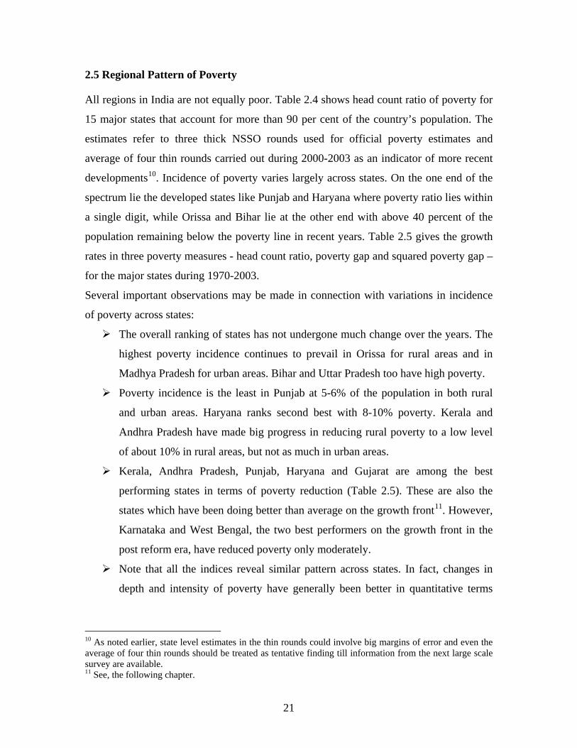
2.5 Regional Pattern of Poverty

All regions in India are not equally poor. Table 2.4 shows head count ratio of poverty for

15 major states that account for more than 90 per cent of the country’s population. The

estimates refer to three thick NSSO rounds used for official poverty estimates and

average of four thin rounds carried out during 2000-2003 as an indicator of more recent

developments10. Incidence of poverty varies largely across states. On the one end of the

spectrum lie the developed states like Punjab and Haryana where poverty ratio lies within

a single digit, while Orissa and Bihar lie at the other end with above 40 percent of the

population remaining below the poverty line in recent years. Table 2.5 gives the growth

rates in three poverty measures - head count ratio, poverty gap and squared poverty gap –

for the major states during 1970-2003.

Several important observations may be made in connection with variations in incidence

of poverty across states:

The overall ranking of states has not undergone much change over the years. The

highest poverty incidence continues to prevail in Orissa for rural areas and in

Madhya Pradesh for urban areas. Bihar and Uttar Pradesh too have high poverty.

Poverty incidence is the least in Punjab at 5-6% of the population in both rural

and urban areas. Haryana ranks second best with 8-10% poverty. Kerala and

Andhra Pradesh have made big progress in reducing rural poverty to a low level

of about 10% in rural areas, but not as much in urban areas.

Kerala, Andhra Pradesh, Punjab, Haryana and Gujarat are among the best

performing states in terms of poverty reduction (Table 2.5). These are also the

states which have been doing better than average on the growth front11. However,

Karnataka and West Bengal, the two best performers on the growth front in the

post reform era, have reduced poverty only moderately.

Note that all the indices reveal similar pattern across states. In fact, changes in

depth and intensity of poverty have generally been better in quantitative terms

10 As noted earlier, state level estimates in the thin rounds could involve big margins of error and even the average of four thin rounds should be treated as tentative finding till information from the next large scale survey are available. 11 See, the following chapter.

22

than those in head count ratio. Thus, benefits of the development process do not

seem to be confined to people near the poverty line.12

As per official poverty estimates, there are several states which have higher

poverty in urban areas than in rural areas; Andhra Pradesh, Kerala, Karnataka,

Madhya Pradesh, Maharashtra, Rajasthan and Tamil Nadu fall in this list. Deaton

and Dreze (2002) find the differential in official estimates of poverty lines

between urban and rural areas to be implausible for several states. Their

alternative estimates of poverty incidence for urban areas are lower than those for

rural areas.

Table 2.4: Head Count Ratio of Poverty for Major Indian States Rural Urban

States 1983 1993-941999-2000

Average of 2000-03 1983 1993-94

1999-2000

Average of 2000-03

Andhra Pradesh 26.53 15.92 11.05 9.80 36.30 38.33 26.63 25.25 Assam 42.60 45.01 40.04 21.40 21.73 7.73 7.47 4.74 Bihar 64.37 58.21 44.30 32.26 47.33 34.50 32.91 27.29 Gujarat 29.80 22.18 13.17 13.14 39.14 27.89 15.59 10.86 Haryana 20.56 28.02 8.27 8.65 24.15 16.38 9.99 10.03 Karnataka 36.33 29.88 17.38 13.28 42.82 40.14 25.25 27.31 Kerala 39.03 25.76 9.38 9.24 45.68 24.55 20.27 15.03 Madhya Pradesh 48.90 40.64 37.06 33.40 53.06 48.38 38.44 40.35 Maharashtra 45.23 37.93 23.72 18.96 40.26 35.15 26.81 25.29 Orissa 67.53 49.72 48.01 46.53 49.15 41.64 42.83 33.93 Punjab 13.20 11.95 6.35 5.49 23.79 11.35 5.75 5.69 Rajasthan 33.50 26.46 13.74 16.28 37.94 30.49 19.85 27.66 Tamil Nadu 53.99 32.48 20.55 18.38 46.96 39.77 22.11 24.90 Uttar Pradesh 46.45 42.28 31.22 33.17 49.82 35.39 30.89 29.92 West Bengal 63.05 40.80 31.85 24.80 32.32 22.41 14.86 15.87 India 45.65 37.27 27.09 25.40 40.79 32.36 23.62 23.97

Source: Planning Commission for 1983, 1993-94 and 1999-2000. Own estimates for average of four thin rounds during 2000-2003.

12 This result holds at a broad group level like aggregate state and might be consistent with intensification of poverty for certain vulnerable groups.

23

Table 2.5: Growth Rates in Poverty Indices: Rural & Urban, 1970-2003

Rural Urban States H PG SPG H PG SPG Andhra Pradesh -4.17 -6.06 -7.36 -1.67 -2.28 -2.79 Assam -1.22 -1.54 -1.85 -3.68 -4.46 -5.11 Bihar -1.10 -2.44 -3.62 -1.96 -3.20 -4.37 Gujarat -3.57 -5.35 -6.68 -3.82 -5.72 -7.41 Haryana -3.42 -4.61 -5.40 -3.98 -6.07 -7.88 Karnataka -2.73 -4.23 -5.35 -1.69 -2.33 -2.88 Kerala -4.72 -6.97 -8.51 -3.37 -5.08 -6.22 Madhya Pradesh -2.44 -3.61 -4.35 -0.75 -1.13 -1.45 Maharashtra -1.15 -2.16 -2.99 -1.30 -1.80 -2.12 Orissa -0.97 -1.73 -2.43 -1.40 -2.06 -2.59 Punjab -3.87 -6.07 -8.08 -4.38 -5.89 -6.99 Rajasthan -2.84 -4.63 -5.97 -1.71 -2.69 -3.60 Tamil Nadu -2.98 -4.58 -5.73 -1.57 -2.21 -2.71 Uttar Pradesh -0.91 -1.69 -2.31 -1.62 -2.60 -3.51 West Bengal -1.98 -3.14 -4.04 -1.49 -2.34 -3.07 All India -1.69 -2.82 -3.70 -1.64 -2.43 -3.10 Source: Own estimates Note: These trend growth rates are computed by fitting exponential function of the type ln(Y) = a + b.T, where Y is the concerned variable and T is time trend. All values are significant. 2.6 Poverty by Social Groups

Table 2.6 gives the poverty ratios by different social groups such as scheduled tribe

(ST), scheduled caste (SC) and other backward classes (OBC) in the Indian social

hierarchy. Incidence of poverty varies widely across social groups. High incidence of

poverty prevails among the scheduled tribe and scheduled caste population, which have

suffered from social and/or economic exclusion for centuries in India13. More than 45%

of households among the ST group are poor while the corresponding number is only 15%

among the non-backward households classified under the ‘others’ category in the table.

13 The ST and SC categories account for a little less than a quarter of the population.

24

Table 2.6: Rural Poverty by Social Groups in Major States: 1999-2000 State ST SC OBC Others Andhra Pradesh 23.07 16.47 9.59 3.4 Assam 39.16 44.97 40.4 39.36 Bihar 59.37 59.3 42.83 26.28 Gujarat 27.5 15.57 11.15 4.58 Haryana 0 17.02 10.82 1.13 Karnataka 24.86 25.67 15.74 11.05 Kerala 25.04 15.61 10.88 4.96 Madhya Pradesh 57.14 41.21 32.32 11.7 Maharashtra 44.2 31.64 21.89 12.78 Orissa 73.1 52.3 39.7 24.01 Punjab 16.64 11.88 6.97 0.56 Rajasthan 24.83 19.52 10.21 6.03 Tamil Nadu 44.58 31.73 14.64 10.64 Uttar Pradesh 34.68 43.38 32.96 17.62 West Bengal 50.05 34.91 20 29.42 All India 45.82 35.89 26.96 14.98

2.6 Poverty by Occupation Class While most poverty estimates for India are based on the NSSO consumption expenditure

distribution data, estimates based on income distribution data are available from sporadic

income distribution surveys conducted by the National Council of Applied economic

Research (NCAER). Table 2.6 reports the head count ratio of poverty estimated by

Pradhan and Roy (2003) using both income and consumption distribution data from

NCAER’s MIMAP (Micro Impacts of Macroeconomic and Adjustment Policy) survey

for 1994-95. The authors use the official poverty lines adjusted for prices. So, these lines

are essentially defined in terms of per capita consumption and not strictly applicable for

income distribution due to the implicit assumption of zero savings at the poverty line.

Hence, poverty estimates based on income are invariably lower than those based on

consumption in Table 2.7. At the national level, income based poverty at 25 per cent is

about 12 percentage points lower than consumption based poverty estimate of 37 per

cent.

More interestingly, the table shows variation of poverty by occupation group. Incidence

of poverty is the highest among wage earning class. It is about 60 per cent higher than

25

that for all groups. An important revelation is that wage earners in both agricultural and

non-agricultural sectors are almost equally poor. Poverty is the least among salaried

group followed by the self-employed in non-agriculture. Poverty among self-employed in

agriculture is higher than average for all groups.

Table 2.7: Head Count Ratio by Occupation Group Using Income and Consumption Distribution Data, 1994-95

Income Based Poverty Consumption Based Poverty Rural Urban All India Rural Urban All India Self Employed in Agriculture 27.4 31.0 27.5 36.8 64.8 37.3 Self Employed in Non-Agriculture 8.1 18.1 13.0 15.1 38.6 26.6 Salaried 6.6 5.3 5.9 18.5 14.2 16.1 Agricultural Wage Earners 42.3 64.0 42.9 55.0 80.0 55.7 Non-Agricultural Wage Earners 43.7 41.6 43.1 53.6 61.0 55.7 Others 15.4 10.4 13.5 29.5 21.4 26.4 All Groups 28.6 14.8 25.1 39.4 28.4 36.6 Source: Pradhan and Roy (2003): The Well Being of Indian Households, MIMAP - India Survey Report, NCAER. Consumption based estimates refer to those based on CE-II comparable to NSSO consumption expenditure concept. Table 2.8 shows distribution of poor by occupation group again based on NCAER’s

MIMAP survey. Agricultural labourers form the largest group among the rural poor

accounting for about 45 per cent of rural poor. The self-employed in agriculture accounts

for another 30 per cent of rural poor population. Thus, about three-quarters of poor

households are primarily dependent on agricultural income. In urban area, the non-

agricultural wage income earners constitute only 25 per cent of urban poor. The self-

employed in non-agriculture account for about a third of urban poor. Although the

incidence of poverty among salaried class is low compared to the average, the poor are

dependent on salary income account for as high as 28 per cent of total urban poor

reflecting large size of salaried group in urban population.

26

Table 2.8: Distribution of Poor by Occupation Group, 1994-95

Head Count Ratio Income Based Poverty Consumption Based Poverty Rural Urban All India Rural Urban All IndiaSelf Employed in Agriculture 31.5 3.5 27.3 30.8 3.8 25.5Self Employed in Non-Agriculture 2.4 29.0 6.4 3.3 32.2 9.0Salaried 3.3 19.7 5.8 6.7 27.6 10.7Agricultural Wage Earners 46.0 11.2 40.8 43.5 7.3 36.5Non-Agricultural Wage Earners 15.2 32.7 17.8 13.5 24.9 15.7Others 1.7 3.9 2.0 2.3 4.2 2.6All Groups 100.0 100.0 100.0 100.0 100.0 100.0

Source: Pradhan and Roy (2003). Note as in Table 2.6. 2.7 Nutrition Although the poverty line for the base year is often based on nutritional intake, the

poverty measures do not directly reflect nutritional deficiency. For example, the official

poverty line in India corresponds to an income level that is just adequate to meet the

calorie norm in 1973-74. This does not mean that all persons above the poverty line meet

the calorie intake norm and all persons below the poverty line are calorie deficient.

Generally speaking, there is an increasing relationship between calorie intake and income

or consumption expenditure (see, Figure: 2.3). Per capita income is a major determinant

of calorie intake, but there are also other factors like household composition, share of

food expenditure, tastes and preferences, availability of types of food that determine food

consumption and energy intake. The ranking of households by per capita income and per

capita calorie intake are not identical. While calorie intake would be highly correlated

with income, it is not a perfect correlation.

27

Figure 2.3:Calorie Intake by Expenditure Class: Rural India 1999-2000

0500

100015002000250030003500

0-22

5

225-

255

255-

300

300-

340

340-

380

380-

420

420-

470

470-

525

525-

615

615-

775

775-

950

950-

Mor

e

Monthly Per Capita Consumption Expenditure

Cal

orie

Inta

ke p

er d

ay

Source: Based on NSSO data

Secondly, the quantified relationship between calorie intake and income need not be very

stable. Income level good enough to meet the calorie norm in the base year need not do

so in subsequent years if consumption pattern changes due to changes in tastes and

preferences, relative prices and other factors. Indeed, there has been considerable

diversification in consumption pattern of people from food to non-food items, within

food group from cereals to non-cereal food items, and within cereals from coarse to fine

cereals. Such changes have meant that households at the poverty line have substantially

less calorie intake than the norms in recent years14. Hence, monitoring of nutritional

intake by itself is of interest.

In an inter-state analysis, Sen (2005) reports that per capita calorie intake in the poverty

line class (e.g., consumption class that contains the poverty line) is the lowest for Kerala

(1389 calories) for rural areas and for Haryana (1457 calories) for urban areas in 1999-

2000. What is also interesting is that the poverty line class in Orissa has the highest

calories for both rural and urban areas, 2117 and 2450 respectively. 14 See, Panda and Rath (2004) for such evidence on India and explanations in terms of consumer behaviour. This paper also demonstrates that there could be situations when reduction in standard poverty measures need not be welfare improving in terms of real consumption.

28

Analysing the food and nutrition security issues, Radhakrishna (2005) notes that the per

capita cereals consumption in India has been on a declining trend during the last three

decades. According to the NSSO data, per capita cereals consumption in rural areas fell

from 15.3 kg per month in 1970-71 to 12.7 kg in 1999-2000 and in urban areas from 11.4

kg to 10.4 kg. This declining trend could be observed in most states with sharp decline of

about 6 kg taking place in Punjab and Haryana. In the year 1999-2000, per capita per

month cereal consumption in a prosperous state like Punjab was 10.6 kg in rural and 9.2

kg in urban areas while it was 15.1 kg in rural and 14.5 kg in urban areas in a backward

state like Orissa.

Rao (2000) observes that the decline in cereal consumption has been greater in rural areas

in those states where improvement in rural infrastructure has made non-cereal food and

non-food consumption items available to rural households. Cereals need might also have

fallen due to reduction in heavy manual work associated with farm mechanisation and

consequent reduction in calorie need. A fall in cereal consumption and calorie intake

need not be interpreted as a sign of welfare deterioration in such situations.

Table 2.9 shows average per capita calorie intake for various expenditure classes of the

population in different years. The per capita calorie intake of the entire population rose

during 1970s but has fallen subsequently despite growth in real per capita total

consumption expenditure. Rural calorie intake particularly has stagnated for all sections

of the population during 1990s due to diversification of the consumption basket. The

improvement in overall urban per capita calorie intake is almost exclusively due to

improvement noticed among top 30 per cent of the population. While per capita calorie

intake of bottom 30 per cent of urban population nearly stagnated, that of middle 40 per

cent declined substantially. Radhakrishna (2005) notes: “In my view, food diversification

is justifiable from a nutritional perspective only if it enhances nutritional status by

increasing the status of micronutrients, even though it may not add much calorie to the

diet. Given the state of knowledge, it is extremely difficult to make any inferences about

the impact of dietary diversification on the nutritional status. However, what is

worrisome is the low per capita calorie intake (1600-1700 k cal/day) of the bottom 30 per

cent which falls short of the required norm” (p.1818). There clearly is a need to increase

energy intake among this section of the population.

29

Table 2.9: Average Per Capita Calorie Intake and Its Growth Rates in India Expenditure Class 1972-73 1977-78 1993-94 1999-2000 K. Cal/day Rural Bottom 30 per cent 1504 1630 1678 1696 Middle 40 per cent 2170 2296 2119 2116 Top 30 per cent 3161 3190 2672 2646 All Groups 2268 2364 2152 2149 Urban Bottom 30 per cent 1579 1701 1701 1715 Middle 40 per cent 2154 2154 2438 2136 Top 30 per cent 2572 2979 2405 2622 All Groups 2107 2379 2071 2156

Source: Radhakrishna (2005)

Incidence of malnutrition is much higher than incidence of income poverty. Abolition of

income poverty need not imply abolition of malnutrition. Micronutrient deficiency of

some type or other is common among both rural and urban people. Vitamin A deficiency

is widely prevalent in rural areas and leads to preventable blindness in acute cases.

National Family Health Survey for 1998-99 shows that about half of pregnant women

suffer from iron deficiency that causes anaemia. This leads to high incidence of low

weight at birth among children, which in turn contributes to child malnutrition. Analysis

by Radhakrishna and Ravi (2004) reveal that the probability of a child falling into

malnutrition decreases with improvement in mother’s nutrition status, mother’s

education, mother’s age and antenatal visit. But, the probability increases if mother is

working. This might largely be reflecting conditions among poor households who are not

able to make proper alternative arrangement for child care when mother is forced to go to

work.

2.8 Human Development Table 2.10 shows human development index (HDI) across states prepared by the

Planning Commission for 1991 and 2001. There is improvement in HDI over time in both

rural and urban areas. Urban-rural differences continue to prevail in all states. Kerala

occupies the top slot in HDI ranking across states, though it is a middle income state.

30

Some high income states like Punjab, Tamil Nadu and Maharshtra perform well in HDI

too.

Table 2.10:Human Development Index - 1991 and 2001 Rural - 1991 Urban - 1991 Rural - 2001 Urban - 2001

States Value Rank Value Rank Value Rank Value Rank Andhra Pradesh 0.344 9 0.473 12 0.377 9 0.416 10Assam 0.326 11 0.555 5 0.348 10 0.386 14Bihar 0.286 13 0.460 14 0.308 15 0.367 15Gujarat 0.380 6 0.532 7 0.437 6 0.479 6Haryana 0.409 4 0.562 3 0.443 5 0.509 5Karnataka 0.367 8 0.523 8 0.412 7 0.478 7Kerala 0.576 1 0.628 1 0.591 1 0.638 1Madhya Pradesh 0.282 15 0.491 11 0.377 9 0.416 10Maharashtra 0.403 5 0.548 6 0.452 4 0.523 4Orissa 0.328 10 0.469 13 0.345 12 0.404 11Punjab 0.447 2 0.566 2 0.475 2 0.537 2Rajasthan 0.298 12 0.492 10 0.347 11 0.424 9Tamil Nadu 0.421 3 0.560 4 0.466 3 0.537 2Uttar Pradesh 0.284 14 0.444 15 0.314 14 0.388 13West Bengal 0.370 7 0.511 9 0.404 8 0.472 8India 0.340 0.511 0.381 0.472 Source: Planning Commission (2002) Health Table 2.11 shows gradual improvement in some selected health indicators over the years

since 1951. Crude birth rate has come down from 41 in 1951 to 34 in 1981 and further to

25 in 2002, while the death rate has fallen faster from 25 in 1951 to 13 in 1981 and 8 in

2002. Infant and child mortality rates too have reduced by more than half to 63 and 19

respectively in 2002. Life expectancy at birth for females stood at 36 years and was lower

than 37 years for males in 1951. It increased faster for females over the last five decades

and is estimated to be 67 years during 2001-06 for females and 64 years for males.

Women have a natural ability to live longer and higher female life expectancy is in line

with those observed for developed countries.

31

Table 2.11: Selected Health Indicators for India

Variable 1951 1981 1991 Latest year1 Crude Birth Rate (Per 1000 Population)

40.8 33.9 29.5 25.0 (2002)

Crude Death Rate (Per 1000 Population)

25.1 12.5 9.8 8.1 (2002)

Infant Mortality Rate (IMR) (Per 1000 live births)

146 (1951-61)

110 80 63 (2002)

Child (0-4 years) Mortality Rate (Per 1000 children)

57.3 (1972)

41.2 26.5 19.3 (2001)

Life Expectancy at Birth (years) Male 37.2 54.1 59.7

(1991-95) 63.9

(2001-06) Female 36.2 54.7 60.9

(1991-95) 66.9

(2001-06) NA: Not Available. 1 The dates in the brackets indicate years for which latest information is available. Source: Economic Survey 2004-05.

Table 2.12 gives variations across states in life expectancy and infant mortality. As is

well known, Kerala’s score in human development is close to that of developed countries.

Life expectancy at birth in Kerala is 72 years for males and 75 years for females. Among

the rest, the states of Punjab, Tamil Nadu and Maharashtra have achieved better life

expectancy for both male and females. Bihar, one of the poorest states has larger life

expectancy for male than Indian average, but not for females. On the other hand, a rich

state like Gujarat has lower record on life expectancy than many other states.

Turning to infant mortality, Kerala again stands out way above other Indian states with a

rate of 9 and 12 for boys and girls respectively. Punjab again has the second lowest infant

mortality rate of 38 for boys. But, it has a very large difference in mortality rate for boys

and girls, the latter being as high as 66. Indeed, Punjab exhibits the highest difference by

gender among all the major states, followed by Haryana. It is worth noting that infant

mortality rate for girls is lower than boys in several states such as Andhra Pradesh,

Karnataka, Maharashtra, Orissa, Tamil Nadu and West Bengal.

The main responsibility for health and family welfare lies with state governments.

Centre supplements the efforts of the states by providing supplementary funds for

national level programmes such as those for communicable diseases, specialised research

32

centres etc. It also coordinates health assistance received from international agencies. On

the whole, health concerns of the rural people have not been reasonably addressed.

Governments have recognised the need for comprehensive primary health care system

and a network of referral systems. They have also laid emphasis on health extension

services with emphasis on preventive rather than curative services. There has been

success in significant reduction in incidence of some communicable diseases or in

complete eradication in some cases. But, the health care system has come under stress in

recent years for various reasons including financial support, manpower availability and

infrastructure provisions. One problem with health sector policies is that there is

multiplicity of public programmes and interventions resulting in thin spread of available

resources. There is also a need for a proper recognition of the complementary role of

private health service for those who can afford it.

Table 2.12: Life expectancy and Infant Mortality Across Major Indian States by Gender

States

Life Expectancy at birth (2001-06)

Infant Mortality Rate (per 1000 live births) 2002

Male Female Male Female Andhra Pradesh 62.8 65.0 64 60 Assam 59.0 60.9 70 71 Bihar 65.7 64.8 56 66 Gujarat 63.1 64.1 55 66 Haryana 64.6 69.3 54 73 Karnataka 62.4 66.4 56 53 Kerala 71.7 75.0 9 12 Madhya Pradesh 59.2 58.0 81 88 Maharashtra 66.8 69.8 48 42 Orissa 60.1 59.7 95 79 Punjab 69.8 72.0 38 66 Rajasthan 62.2 62.8 75 80 Tamil Nadu 67.0 69.8 46 43 Uttar Pradesh 63.5 64.1 76 84 West Bengal 66.1 69.3 53 45 India 63.9 66.9 62 65

33

Education

There are large differences in literacy rate among the states as revealed by Table 2.13. It

varies from 91 per cent in Kerala to 47 per cent in Bihar in 2001. Maharashtra and Tamil

Nadu have achieved 77 and 73 per cent literacy rate compared to the national average of

65. Punjab, Gujarat, West Bengal, Haryana and Karnataka are other states that have more

than national average literacy rates. Substantial gender gap in literacy is again evident

across states. In none of the states in Table 2.13 female literacy is higher than male

literacy. Kerala has the lowest gap with 6 percentage points difference between male and

female literacy rates while Rajasthan has the highest with 32 percentage points.

Table 2.13 Literacy Rate for Major States

in India (2001 Census) (in %) States Persons Males Females Gender Gap* Andhra Pradesh 61.1 70.9 51.2 19.7 Assam 64.3 71.9 56.0 15.9 Bihar 47.5 60.3 33.6 26.8 Goa 82.3 88.9 75.5 13.4 Gujarat 70.0 80.5 58.6 21.9 Haryana 68.6 79.3 56.3 22.9 Himachal Pradesh 77.1 86.0 68.1 17.9 Jammu & Kashmir 54.5 65.8 41.8 23.9 Karnataka 67.0 76.3 57.5 18.8 Kerala 90.9 94.2 87.9 6.3 Madhya Pradesh 64.1 76.8 50.3 26.5 Maharashtra 77.3 86.3 67.5 18.8 Orissa 63.6 76.0 51.0 25.0 Punjab 70.0 75.6 63.6 12.1 Rajasthan 61.0 76.5 44.3 32.1 Tamil Nadu 73.5 82.3 64.6 17.8 Uttar Pradesh 57.4 70.2 43.0 27.3 West Bengal 69.2 77.6 60.2 17.4 India 65.4 76.0 54.3 21.7

Literacy rate is defined as number of literates as a percentage of population in the age group 7 years and above.

Source: www.censusindia.net

34

Like health, educational development in the public sector is the primary responsibility of

state and local governments under the Indian constitution. The Central government plays

a supplementary role in national level policy formulation and financial help for

undertaking some programmes initiated by it. There has been rapid progress in spread of

literacy and access of children to schools reflected in enrolment rates in recent decades,

particularly in some of the educationally backward states. High drop out rate in schools is

a major problem in providing a minimum level of education to all children. There has

been an improvement in recent years in the retention of students from primary schools to

middle schools.

Improvement in quality of education in schools is an important issue that needs

urgent policy attention. This requires adequate provision of number of teachers and

infrastructure in schools. A regulatory framework for maintaining standards needs to be

introduced so that service providers are made accountable to local governments, NGOs

and community organisations.

A universal education programme called Sarva Shiksha Abhijan has been initiated

to provide eight years of schooling to all children in the age group 6-14 years by 2010.

Apart from improving general coverage to all children, it places emphasis on correcting

some major weaknesses like bridging the large gender gap in educational attainment and

in universal retention of children up to the middle school level.

2.9 Consumption Inequality The NSSO data have also been used to estimate the concentration index (Gini Coefficient

or Lorenz Ratio) for rural and urban population of the country. The estimates in nominal

terms are shown in Figure 2.3. Urban inequality in consumption expenditure is

invariably larger than rural inequality. There is a tendency of a reduction in inequality

within the rural sector from around 0.30 in early 1970s to 0.27 in recent years15. It might

be noted in this context a point made by Sen and Himanshu (2004) that comparison of

inequality measures directly computed from NSSO data for 50th round (1993-94) and 55th

round (1999-2000) are misleading due to the fact that 50th round used 30-day recall

15 Statistical tests, too, confirm a reduction in rural inequality in nominal terms without adjustment for differential inflation rates faced by different income classes.

35

period and 55th round 365-day recall period for durables like clothing etc. They find that

measured inequality with 365-day recall is lower than that with 30-day recall by as much

as 5 Gini points. There seems to have been an increase in inequality during 2001-03

compared to 1999-200016.

So far as urban areas are concerned, there is no noticeable long-term change in

consumption distribution measured by Gini concentration ratio during 1970-2003. The

Gini ratio has generally fluctuated within a range of 0.34 to 0.38 in urban India during

this period. Again, there seems to have been an increase in urban inequality after 1999-

2000.

25

27

29

31

33

35

37

39

1959

-60

1960

-61

1961

-62

1963

-64

1964

-65

1965

-66

1966

-67

1967

-68

1968

-69

1969

-70

1970

-71

1972

-73

1973

-74

1977

-78

1983

-84

1986

-87

1987

-88

1988

-89

1989

-90

1990

-91

1991

1992

1993

-94

1994

-95

1995

-96

1997

1998

1999

-00

2000

-01

2001

-02

2002

2003

Rural Urban

Figure 2.4: Gini coefficient in size distribution of per capita consumption expenditure

Table 2.14 indicates the growth rates in Gini coefficients and real mean consumption for

rural and urban areas for major states. Mean consumption has grown in all states except

for Assam where the rural growth is not significant. The pattern of poverty reduction

noticed across states broadly follows the growth in mean consumption. Rural inequality

has also fallen in most states, the exceptions being Kerala, Madhya Pradesh and Uttar

Pradesh where changes are not significant. Consistent with national level result, urban

16 The NSSO data are comparable since 1999-2000.

36

inequality does not show a significant change in any state considered here except for two

sattes, Andhra Pradesh and West Bengal where there is a significant rise.

Table 2.14: Growth Rates of real MPCE and Gini Coefficients, 1970-2003

Rural Urban States GINI MEAN GINI MEAN Andhra Pradesh -0.31 1.53 0.29 1.08 Assam -0.32 0.21* -0.11* 0.95 Bihar -0.88 0.47 -0.15* 1.03 Gujarat -0.42 1.35 0.06* 1.6 Haryana -0.44 0.86 -0.17* 1.31 Karnataka -0.51 0.98 -0.07* 0.94 Kerala -0.14* 2.24 -0.1* 2.01 Madhya Pradesh 0.02* 0.47 0.00* 0.48 Maharashtra -0.58 1.25 -0.19* 0.72 Orissa -0.25 0.46 -0.09* 0.95 Punjab -0.44 0.86 -0.26* 1.27 Rajasthan -0.98 0.82 -0.1* 0.76 Tamil Nadu -0.21 1.39 0.14* 0.91 Uttar Pradesh -0.18* 0.41 -0.08* 1.02 West Bengal -0.35 0.79 0.15 0.71

* Not Significant; Source: Own estimates

2.10 Growing rural-urban disparity There is, however, one aspect of distribution that needs to be stressed for policy purpose.

Difference in rural-urban mean consumption at current prices has accentuated during

post-reform period (Table 2.15). At the national level, urban mean was 67% higher than

rural mean on an average in the 50th-52nd rounds of NSSO. This difference has moved up

to 87% during 57th-59th rounds. It is seen across the board for all states except Bihar and

Maharashtra where the urban-rural inequality virtually remains the same. Sen and

Himanshu (2004) find that the urban-rural gap increased more sharply during 1990s when

nominal average consumption levels are corrected for relative price rises. Cereal prices,

which have a large weight in consumer price index of agricultural labourers, increased

faster in early 1990s than during the 1980s.

37

Table 2.15: Urban-Rural Mean Consumption Ratio (at current prices)

States

Average 50-52 Rounds

Average 57-59 Rounds

Andhra Pradesh 1.625 1.732 Assam 1.667 1.702 Bihar 1.610 1.606 Gujarat 1.414 1.763 Haryana 1.260 1.510 Karnataka 1.599 1.823 Kerala 1.186 1.413 Madhya Pradesh 1.475 1.909 Maharashtra 2.071 2.062 Orissa 1.824 2.236 Punjab 1.365 1.382 Rajasthan 1.394 1.480 Tamil Nadu 1.496 1.797 Uttar Pradesh 1.395 1.692 West Bengal 1.667 1.972 All-India 1.672 1.875

Inequality enhancing effects in the early phase of growth process postulated in some

growth models does not generally seem to have operated in rural or urban India on a

long-term basis. Direct policy measures aimed at social justice could have played a role

in neutralizing the predictions of theoretical growth models. Such measures include large-

scale adoption of direct poverty alleviation programmes and social sector expenditure,

among others, discussed later. NSSO survey data admittedly do not adequately cover the

very well to do sections and might have a tendency to under estimate the relative share of

the rich. Even then, the democratic political process possibly does ensure that the poor do

receive some benefit from the overall development process within rural or urban areas.

We end this chapter with an overall observation on the interactions of growth, poverty

and inequality. We noted earlier that there was no trend decline in incidence of poverty in

India till mid-1970s. Given the low per capita growth and the near invariance of

distribution parameter for more than two decades, the poor did not gain much in absolute

terms to make a long-term impact on poverty. The fall in poverty incidence was visible

after mid-1970s when the economy moved up to a phase of higher economic growth of 5

per cent or above.

38

2.11 Conclusion

Poverty was widespread in India at the time of independence. The national government

focused on a process of economic growth and poverty reduction through the initiation of

the Five Year Plans in 1951. Incidence of poverty, however, did not show a visible

downward trend for more than two decades. It started to fall from about 55 per cent in

1973-74 to 45 per cent in 1983 and further to 39 per cent in 1987-88. In recent years,

official estimates based on large sample survey of households show a reduction in

incidence of poverty from 36 per cent in 1993-94 to 26 per cent in 1999-2000. Data for

four thin rounds available since 1999-2000 too indicate that about a quarter of India’s

population continue to live in absolute poverty.

Analysis of long-term data show that there has been significant reduction in poverty in all

major states of India during 1970-2003. The depth and intensity of poverty have fallen at

a faster rate than the head count ratio. In recent years, poverty seems to be getting

concentrated in Eastern and Central parts of India and among the Scheduled Tribes and

Scheduled Caste population. Mean consumption expenditure show significant rise in

rural and urban areas of all major states except rural Assam. Inequality too has fallen in

rural areas of most states, though urban inequality in most states has not changed

significantly. The urban-rural disparity in mean consumption has accentuated since early

1990s.

Incidence of undernutrition and malnutrition in India is higher than incidence of income

poverty. Micronutrient deficiency of one form or another seem to be common among a

large section of the population. India lags behind in terms of human development

indicators such as achievements in education and health fields in international

comparison.

39

Chapter 3 Changes in Income and Employment1

3.1 GDP Growth A long-term perspective on the post-independence growth process in the Indian economy

could be obtained by looking at the national income growth rate since 1951. Table 3.1

presents average annual growth rates in national income for three broad sectors -

agriculture, industry and service - for various periods spanning over 1951-2004. The

Indian economy grew at an average rate of 3.5 per cent per annum for about 3 decades till

1980. With a population growth rate of about 2%, this meant a long trend growth rate of

only about 1.5% in per capita terms. However, a break through occurred around 1980 and

the trend growth rate improved to above 5 per cent after that2. A high GDP growth

coupled with marginal slow down in the population growth rate has resulted in per capita

income growth rate of above 3.5% per annum. An increase in average level of living of

this order for about quarter of a century no doubt marks a break from the earlier trend.

The acceleration of the economy during 1980s caused by an expansionary fiscal policy

was not sustainable and led to a balance of payments crisis in 1991. Post-reform GDP

growth rate accelerated to above 7% during the triennium ending 1997-98 but has come

down to about 6% later. The improvement in growth rate has been driven mostly by the

service sector. The growth rate achieved in the post-reform period appears to be a

sustainable one on a long-term basis. There is overall macroeconomic stability as

indicated by factors such as low inflation, stable exchange rate, adequate foreign

exchange reserves, low short-term external debt and sufficient foodgrains stocks. Areas

that have been causing concern for growth and stability are fiscal imbalances and near

stagnant investment rates.

The economy achieved an average GDP growth rate of about 6 per cent despite several

shocks like the East Asian crisis, border tension, the Iraq war, oil price rise and a major

drought in recent years. It seems to have acquired new strength compared to the fragile 1 This chapter is written by Manoj Panda. 2 Statistical tests by Virmani (2004) distinguish only two phases in Indian economic growth with 1980-81 as the dividing line.

40

situation in early 1990s when it broke down due to oil price rise in the wake of the Gulf

war. India has been among the fastest growing economies during the last decade. While

the achievement in the post-independence period is no doubt commendable in

comparison with the colonial period, India lags behind several newly industrialized

countries in Asia. Indian observers rightfully expect the economy to grow more rapidly

over the coming years. The optimism about a higher growth potential gets reflected in the

Planning Commission’s growth target of 7-8 per cent per annum. It is being recognized in

international circles that India is steadily progressing on the path to become a major

economy in the world3.

Table 3.1: GDP and Per Capita GDP Trend Growth Rates: India, 1950-2004 1950-70 1970-80 1980-90 1990-2000 1992-2004

GDP growth by major sectors Agriculture 2.17 1.80 3.07 2.95 2.31 Industry 6.13 4.36 6.67 6.12 5.96 Services 4.61 4.53 6.65 7.72 7.90 GDP total 3.64 3.34 5.37 5.94 5.93

Per capita GDP growth by major sectors Agriculture 0.11* -0.46 0.94 0.99 0.46 Industry 4.06 2.10 4.54 4.16 4.11 Services 2.55 2.28 4.51 5.76 6.04 Total 1.57 1.08 3.24 3.98 4.07

* Not significantly different from zero.

3 See, for example, Wilson and Purushothaman (2003): “Dreaming With BRICs: The Path to 2050”, Global Economics Paper No. 99, Goldman Sachs.

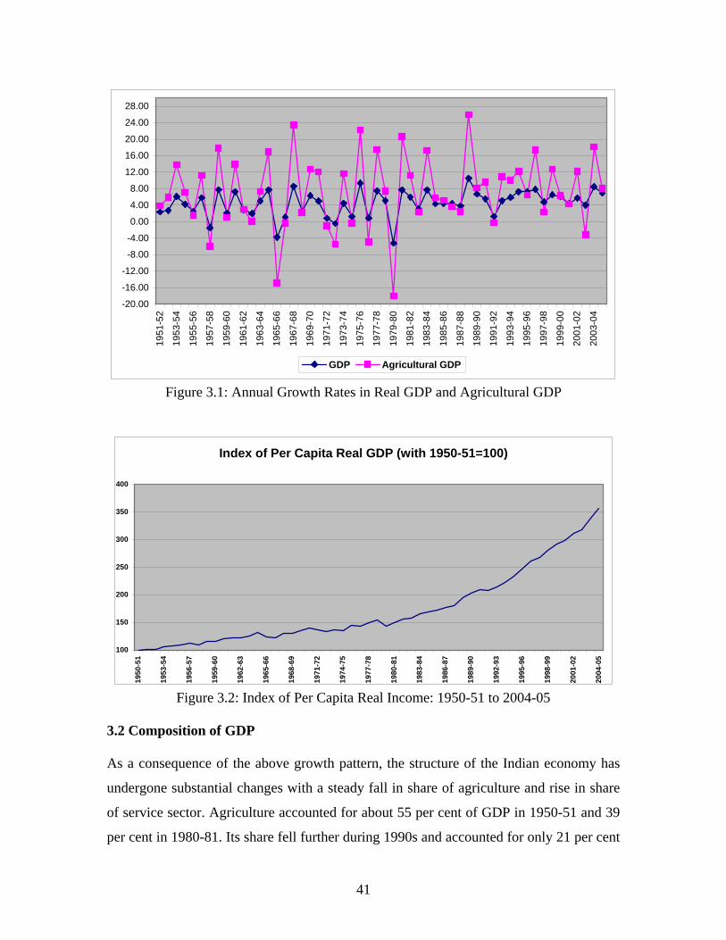
41

-20.00

-16.00

-12.00

-8.00

-4.00

0.00

4.00

8.00

12.00

16.00

20.00

24.00

28.00

1951

-52

1953

-54

1955

-56

1957

-58

1959

-60

1961

-62

1963

-64

1965

-66

1967

-68

1969

-70

1971

-72

1973

-74

1975

-76

1977

-78

1979

-80

1981

-82

1983

-84

1985

-86

1987

-88

1989

-90

1991

-92

1993

-94

1995

-96

1997

-98

1999

-00

2001

-02

2003

-04

GDP Agricultural GDP

Figure 3.1: Annual Growth Rates in Real GDP and Agricultural GDP

Index of Per Capita Real GDP (with 1950-51=100)

100

150

200

250

300

350

400

1950

-51

1953

-54

1956

-57

1959

-60

1962

-63

1965

-66

1968

-69

1971

-72

1974

-75

1977

-78

1980

-81

1983

-84

1986

-87

1989

-90

1992

-93

1995

-96

1998

-99

2001

-02

2004

-05

Figure 3.2: Index of Per Capita Real Income: 1950-51 to 2004-05

3.2 Composition of GDP As a consequence of the above growth pattern, the structure of the Indian economy has

undergone substantial changes with a steady fall in share of agriculture and rise in share

of service sector. Agriculture accounted for about 55 per cent of GDP in 1950-51 and 39

per cent in 1980-81. Its share fell further during 1990s and accounted for only 21 per cent

42

of GDP in 2004-05. The share of industry (including construction), which was only about

14 per cent in early 1950s, rose to 24 per cent in 1980-81 reflecting the high emphasis put

on the industrialization process during the sixties and seventies. Industry’s share has

stagnated just above a quarter of GDP since 1990 except for a few years during mid-

1990s. The composition of GDP has been continuously moving in favour of services,

which accounted for about 30 per cent of national income in 1950-51 and 41 per cent in

1990-91. Services currently account for 52 per cent of GDP in India. While the structural

change away from agriculture is broadly consistent with international experience for

countries at similar phase of development noted in the pioneering studies by Kuznets and

Chenery, the composition within non-agriculture in India is somewhat different. It differs

from the classical pattern in so far as growth of Indian economy is largely driven by

service sector since 1990 and not by manufacturing.

Table 3.2: Composition of GDP by major sectors Year Agriculture Industry Services

1950-51 56.35 14.14 29.51 1960-61 46.50 19.36 34.13 1970-71 45.90 20.57 33.53 1980-81 38.86 24.49 36.64 1990-91 31.27 27.64 41.10 2000-01 24.62 26.60 48.78 2004-05 21.13 27.15 51.72

The falling share of agriculture has an important effect on reducing short-term

fluctuations in the economy in recent decades. The Indian economy is described in the

textbooks as a 'vagary of monsoons' in the past, annual fluctuations in GDP growth rate

being mostly been driven by weather effect on the agricultural sector. For example, GDP

used to fall in absolute amount leading to negative growth in drought years like 1965-67,

1972-73 or 1979-80 (Figure 3.2). The economy is no longer as much driven by

agriculture and has been able to absorb shocks in rainfall more smoothly in recent years

due to falling share of agriculture along with development of irrigation facilities. There

has been no negative growth rate in total GDP since 1980-81 despite very low rainfall in

years like 1987-88 or 2002-03, though agricultural output has fallen in these years.

Indeed, real GDP has grown by 4 per cent or above in all the years during last two

43

decades except the crisis year of 1991-92. This new lower limit on annual growth rates is

another feature of the dynamism and strength of the economy.

3.3 Developments within Agriculture Soil and climatic conditions in India are generally suitable for growing foodgrains and

the country has natural comparative advantage in its production of foodgrains. Yet, India

was not self sufficient in foodgrains production to meet domestic demand till mid-1970s.

It depended on imports which preempted scarce foreign exchange availability required

for non-competitive imports like capital goods and raw materials to lay the foundations

for industrialization. Moreover, large-scale imports of grains at times touching 10 million

tonnes caused an upward pressure on world grain prices4. Hence, achieving self-

sufficiency in foodgrains production became a major goal of development planning.

Prior to independence, there was no visible technological change in agriculture and

production was on the whole stagnant over a long period except for a few export oriented

commercial crops like jute and tea where the colonial interest was directly involved. The

overall institutional set up was not conducive for long term investment and technological

change. A large part of cultivated area did not belong to the tiller due to prevalence of

intermediary systems like zamindars and jagirdars. Producers had little incentive for

large investment on land because of lack of security of tenure. Hence, there was an

emphasis on agrarian institutional changes such as land reform after independence5. Land

reforms in India involved two main components: (a) abolition of intermediaries soon after

independence so that land belongs to the tillers, (b) imposition of ceiling on land

ownership and distribution of surplus land among the landless. As it turned out in

practice, the first component was by and large successful and tillers, accounting for about

40 per cent of total cultivated area, became actual owners. But, the second component

met with very limited success due to political dominance of large farmers as well as legal

loopholes involving numerous exemptions to land ceiling. On the whole, less than 2 per

cent of cultivated area could be acquired as surplus for distribution among the landless

(Rao, 1992). There was, however, subdivision of landholdings over time due to

4 International trade in rice is particularly thin. Quantum of public stocks of rice with the Indian government in recent years is more than volume of world trade. 5 See, Rao (1992) for a review of agricultural policy after independence.

44

population growth and some of the large landholdings naturally came within the legal

ceilings a decade or two after enactment of the law.

By mid-1960s, there was a general recognition of the need for shift in policy emphasis to

technological up-gradation for meeting the food needs of the country. The ‘green

revolution’ introduced in late 1960s and early 1970s involved adoption of high yielding

varieties (HYV) seeds and chemical fertilisers along with large volume of public

investment for expansion of irrigation capacity. Given the complementary nature of

public and private investment in agriculture, there was a steep rise in total agricultural

investment. Government procurement operations guaranteed minimum support price to

farmers in parts of the country (Box 3.1). These policies led to an increase in net

production of foodgrains from 67 million tones (MT) in 1959-60 to 96 MT in 1979-80

and further to 187 MT in 2003-04 (Table 3.3)6. Initiation of the green revolution in

developed regions, where consumption needs of foodgrains were already nearly met, led

to large expansion in marketed surplus and government stocks. The success of green

revolution, particularly in North-West part of India, turned the country to a net exporter

of foodgrains during most of the years since mid-1990s. As Table 3.3 shows government

has all along being an active participant in procurement of marketed surplus from farmers

and distribution to consumers through its own net work.

Table 3.4 reveals that total area under principal crops has increased marginally in recent

decades, though area allocation within agriculture has changed from foodgrain crops in

favour of non-foodgrain crops such as cotton, edible oils and sugar cane. Index number of

agricultural production has more than doubled after 1970-71. This increase in output can

be mostly attributed to rise in yield per hectare rather than expansion of area. In

particular, the area under foodgrains has changed very little since 1980-81 and foodgrains

output growth in recent decades is almost entirely due to increase in yield per hectare.

Area under non-foodgrain crops has increased by about 30 percent in 2003-04 over 1970-

71 while yield per hectare of these crops has increased by 60 percent during the same

period.

6 Gross production of foodgrains has crossed 200 million tones in recent years since 12.5 per cent allowance is made for seed, feed and waste in official figures.

45

Table 3.3: Net Production, Imports, Availability, Procurement

and Public Distribution of Food Grains (Million Tonnes)

Year

Net Produc- tion

Net Imports

Net Availabi-

lity

Per capita net availability per

day (grams)

Procure- ment by

government

Public Distribu-

tion

1960 67.5 5.1 71.2 449.6 1.3 4.9 1970 87.1 3.6 89.5 455.0 6.7 8.8 1980 96.0 -0.3 101.4 410.4 11.2 15.0 1990 149.7 1.3 144.8 476.4 24.0 16.0 1995 167.6 -2.6 166.7 495.4 22.6 15.3 2000 183.6 -1.4 168.3 454.4 35.6 13.0 2001 172.2 -2.9 157.0 416.2 42.6 13.2 2002 186.1 -6.7 189.5 494.1 40.3 18.1 2003 152.9 -5.5 170.1 437.6 34.5 22.5

2004 P 186.8 -6.5 183.6 463.3 41.1 N.A. Notes: Production figure relate to agricultural year (July to June); 1960 figure relate to 1959-60 and so on. Net production has been taken as 87.5% of gross production, 12.5% being provided for seeds, feed requirement and waste. Net availability includes changes in stocks with traders, producers and consumers and so is not strictly representative of actual consumption. P: Provisional. Source: Economic Survey, 2005-06

Table 3.4: Index Number of Agricultural Production, Area and Yield

(1981-82 =100.0) 1970-71 1980-81 1990-91 2000-01 2001-02 2002-03 2003-04 2004-05Agricultural Production Foodgrains 87.9 104.9 143.7 158.4 172.5 140.4 172.1 164.7Non-foodgrains 82.6 97.1 156.3 178.2 189.5 167.2 196 203.7All Commodities 85.9 102.1 148.4 165.7 178.8 150.4 181 179.2Area Under Principal Crops Foodgrains 97.9 99.8 100.7 95.4 96.7 89.7 93.9 94.7Non-foodgrains 91.1 99.4 120 127 127.6 115.6 119.9 130.8All Commodities 96.3 99.7 105.2 102.7 103.9 95.7 99.9 103Yield Of Principal Crops Foodgrains 93.2 105.1 137.8 152.8 164.1 143.2 168.3 160.8Non-foodgrains 91.4 99.2 128 133.2 139.1 126.3 149 149.7All Commodities 92.6 102.9 133.8 144.4 153.3 135.7 160 156Source: Economic Survey, 2005-06.

46

Box 3.1: Government Intervention in Foodgrains Market

Government of India has been intervening in the foodgrains market for several decades. Since the poor spent bulk of their total expenditure on foodgrains, availability of grain at a cheap price was critical for protecting and improving their real level of living. Cheap ‘wage good’ was also considered important to realize surplus for industrialization. In the pre-green revolution period when excess demand prevailed in the foodgrains market, terms of trade was generally favourable to agriculture. Government intervention then was primarily aimed at procuring grains from farmers at lower than market price and distributing the same to urban consumers at a cheaper rate. As he excess demand situation vanished in the post-green revolution period, there was a need to ensure that prices did not fall below the normal cost of production and the producers received an adequate return. To reconcile the twin objectives of protecting the consumers as well as the producers, government intervened in the market the form of large-scale foodgrains procurement from the farmers in the surplus region at a minimum support price. The increased availability of grains from procurement operations helped to extend the distribution mechanism to rural areas and initiate the food for work programme that provided employment to the poor (discussed later). Foodgrain market intervention was thus one of the instruments that tried to ensure that the gains from the green revolution were shared by both producers and consumers.

The procured grains, mostly rice and wheat, by a public sector enterprise

called Food Corporation of India are partly used to maintain a buffer stock and partly distributed through a wide net work of public distribution system (PDS) at fair prices. If market price of foodgrains rises beyond a ‘desirable’ limit in some years, the government releases grains to the market in a selective manner to control the price. The government incurs large amount of food subsidy due to such intervention. The public distribution system has recently been targeted towards the poor with differential prices for the poor and non-poor. The procurement operations have not been equally effective in all parts of the country. The minimum support price system has introduced distortions in crop area allocation in favour of rice and wheat in states like Punjab, which pioneered the Green Revolution but faced ground water constraints in later years.

47

The change in cropping pattern is largely due to changing demand pattern, though

farmers’ allocation decisions have been partly distorted due to the bias in agricultural

price support policy in favour of rice and wheat in the green revolution areas. Huge

buffer stocks of cereals built up by the government reaching 60 million tonnes in some

months in 2002 points towards limited future consumption growth potential for cereals

and the need for further agricultural diversification. It is normally observed that

household demand for foodgrains reaches a near plateau like situation after certain

income level. Engel’s Law propounded long ago states that, as income of a typical

household rises, it demands less of foodgrains and more of other food items in

proportionate terms. Total foodgrains demand in India will continue to grow slowly in

future in response to population pressure and upward mobility of low-income groups.

Rao (1992) mentions several important implications of the green revolution and

associated new technology. First, while the new agricultural technology has been land

and labour saving, application of other inputs like irrigated water, fertilizers and

pesticides has increased substantially. Second, use of HYV seeds and intensive fertilizer

has led to an increase in response of output to water. This has led to a greater instability

in output for a given variability in rainfall or moisture conditions. Third, the green

revolution, which started in relatively less labour abundant areas such as Punjab and

Haryana, induced mechanization and expected large labour absorption due to land-saving

nature of the technology did not take place. Notwithstanding large out-migration of

labour from less developed and highly populated area like Bihar to Punjab, there was on

the whole a fall in elasticity of employment with respect to agricultural output.

Fall in public investment in agriculture during 1980s and subsequent near stagnation after

the reforms has been a matter of concern (Figure 3.3). Chadha (2003) shows that public

sector accounted for 54 per cent of agricultural total gross capital formation in 1980-81,

but this share fell to about 30 per cent in 1990-91 and further to a quarter by end of

1990s. He points out that this has led to net irrigated area remaining stagnant around 53-

55 million hectares since mid-1990s. Agricultural public investment in the NAS mostly

covers expenditure on medium and major irrigation systems. Chand (2002) constructs a

broad series of rural investment by extending it to include investment in rural roads,

48

markets, storage and rural electrification which are important for agricultural

development. He finds that this broad series also indicate a declining trend. Figure 3.6

shows that total capital formation in agriculture has picked up in recent years primarily

due to private investment component. Despite this investment increase, agricultural

growth has stagnated which reflects rising capital intensity of agricultural production.

One reason for the capital cost increase is the depletion in water table in areas dependent

on ground water.

Figure 3.3: Gross Capital Formation in Agriculture

by Public and Private Sectors at 1993-94 Prices

Gross Capital Formation in Agriculture

0

2000

4000

6000

8000

10000

12000

14000

16000

18000

20000

1970

-71

1972

-73

1974

-75

1976

-77

1978

-79

1980

-81

1982

-83

1984

-85

1986

-87

1988

-89

1990

-91

1992

-93

1994

-95

1996

-97

1998

-99

2000

-01

2002

-03

Rs.

in C

rore

s

GCFAgr (Total) GCFAgr (Public) GCFAgr (Private)

`

Source: Based on National Account Statistics Back Series1950-51 to 1992-93 and National Account Statistics, 2005.

Consumption of fertilizers has increased steadily from 2.2 million tones in 1970-71 to

12.5 MT in 1990-91 and to 18.3 MT tones in 2004-05. Average fertilizers consumption

was about 97 kg per hectare in 2004-05 with large variations among states 192 kg for

Punjab and 37 kg in Rajasthan. Government provides large amount of fertilizer subsidy

by way of meeting the difference between administered selling price and cost of

production. It stood at about Rs.16000 crores in 2004-05 which translates to about 3 per

cent of agricultural GDP. Public irrigation is also highly subsidized and irrigation charges

are not able to recover even the operating cost. There is a realization that the fall in

agricultural public investment noted above is partly caused by diversion of a growing

49

volume of resources to input subsidies. Overall, the agricultural sector would benefit by

reallocating public expenditure from input subsidies to investment. In recent years,

government has initiated measures to streamline and control the subsidies.

Indian farmers have traditionally tried to supplement their crop income with earnings

from livestock produce, which also safeguards against large year-to-year fluctuations in

crop income. India has become the largest producer of milk in the world in recent years.

Accounting for about a quarter of GDP in agriculture and allied sector, livestock has

recently emerged as the most important sub-sector within it. The income generated in this

sector gets more equitably distributed since livestock ownership is skewed in favour of

small farmers in India. Further, women account for a majority of the workforce in

livestock.

Given the large variability in climate and soil conditions in the country, India is suitable

to produce a wide range of high value, but employment intensive, horticulture crops

including floriculture. Commercial horticulture targeting the exports markets with good

profit opportunities could attract educated entrepreneurs to agriculture and change the

nature of agricultural operations. It is necessary to develop modern infrastructure such as

cold storage for preservation, refrigerated transportation, grading and quality control for

these emerging sectors.

3.4 Industry Industrial deregulation and trade reforms introduced changes in the overall environment

and organisational structure in Indian industry which has witnessed considerable

structural changes after reforms. Competition has also forced Indian firms to give priority

attention to improvement in product quality, reliability and durability. Foreign technology

purchase has expanded significantly in the form of equity linked technology collaboration

route.

Industrial growth rate has remained sluggish for most of the years after the reforms

except for the period 1994-97. Industrial growth was led by the capital goods sector

during the 1980s, but not so after the 1991 reforms. The capital goods sector saw the

highest tariff reduction and consequent import expansion led to its slowdown after the

50

reforms. The industrial growth process has been more evenly dispersed across consumer

goods, capital goods and intermediates in the post-liberalization period (Figure 3.4).

7.5

12.0

6.2

14.2

4.45.3

6.4 6.58.5

5.8

0

4

8

12

16

Bas

icgo

ods

Cap

ital

good

s

Inte

rmed

iate

good

s

Con

sum

erD

urab

les

Con

sum

erN

on-

dura

bles

1982-1990 1991-2004

Figure 3.4: Average Annual Growth Rates in Index Number of Industrial Production by Used Based Sectors

Source: Own estimates. There is a large unregistered sector employing less than 10 labourers (20 labourers

without electricity) that is engaged in manufacturing activities in India. Labourers are

normally informally employed in the unregistered sector. Its share has fluctuated in a

narrow range of 32.5 and 35.5 per cent of total manufacturing GDP since 1993-94

(Figure 3.5). Thus, the earlier anticipation of large push in growth of unregistered sector

after the reforms has not been evident from the national accounts data. The construction

sector has grown faster since 1992 than during the earlier period. Improvement in road

connectivity across major cities as well as within rural areas has received priority in

public investment in recent years. Being a labour intensive sector, growth in construction

sector has been a major factor behind expansion in demand for labour.

51

2022242628303234363840

1993-94

1994-95

1995-96

1996-97

1997-98

1998-99

1999-00

2000-01

2001-02

2002-03

2003-04

Share of unregistered segment in manufacturing

Figure 3.5: Percentage Share of Unregistered Sector in Total Manufacturing Value Added

Source: Based on National Accounts Statistics. 3.5 Service The service sector has been growing at a faster rate than agriculture or industry during

recent decades. It now accounts for more than half of total GDP generated in the country.

Figure 3.6 depicts the average growth rates for the various components of the service

sector during 1980s and 1990s. Communication has been the fastest growing component

within the service sector during the post-liberalisation phase. With an average growth rate

of about 19 per cent per annum, its contribution to real GDP has increased from 1.2 per

cent in 1993-94 to 4.3 per cent in 2003-04. Other service sectors that have recorded

higher growth since 1992 than during the 1980s include trade, hotels and restaurants,

transport (other than railways) and other services.

On the other hand, there was deceleration in growth of public sector dominated sectors

like railways, and banking and insurance. The service growth during 1980s was led by

banking and insurance sector which, despite the deceleration, continues to witness

relatively high growth due to the entry of private players in the financial market during

post-liberalization phase. Public administration and defense sector continues to grow

after reforms at about the same rate as in 1980s. While government placed restrictions on

expansion of new government jobs in the 1990s due to overstaffing, it had to spend more

in real terms on existing employees due to salary hike.

52

Questions have been raised about the sustainability of service led growth in India.

Virmani (2004) examines whether the share of services in Indian GDP is excessively

high compared to other countries at similar stage of development. He undertakes a cross-

country regression of the average share of service during 1992 to 2000 on the average per

capita GDP at constant PPP and derives a normative value of the service share

corresponding to different income levels. He finds India’s actual share of service sector in

GDP is almost normal in relation to the predicted value; it was just one percentage more

during this period.

0

5

10

15

20

cons

truc

tion

Trad

e

Hot

els

and

Res

taur

ant

Rai

lway

s

Tran

spor

t by

othe

r mea

ns

Stor

age

Com

mun

icat

ion

Ban

king

and

Insu

ranc

e

Rea

l Est

ate

Publ

icA

dmin

istr

atio

nan

d D

efen

ce

Oth

er s

ervi

ces

1981-91 1992-03

Figure 3.6: Annual average growth rates in construction and service sectors

While the service sector growth in India seems to be in line with current international

experience, the divergence of income and employment pattern does pose a main problem

for India. With majority of population still depending on agriculture, the need for higher

growth of agriculture and agro-based industries cannot be denied for poverty reduction. It

is pertinent here to draw attention to interdependence of sectors from a growth

perspective. Analysing input-output coefficients during 1968-69 to 1993-94, Sastry et.al

(2003) report that the dependence of agriculture on industry and service sectors as

suppliers of raw material has gone up, but dependence of industry or service on

agriculture has gone down. Thus, agriculture has stronger backward linkages with

53

industry and service sectors. They find that agricultural sector has a larger effect on

overall growth because of stronger demand linkages with other sectors in the economy.

Despite its larger share, service sector growth does not play a major role in inducing

growth in other sectors.

3.6 Sources of Growth

Expansion in volume of production could take place either by increasing the quantum of

inputs used in the production process or by increasing the productivity of the inputs used.

Productivity growth is recognized as a major source of economic growth in various

economies. Total output growth can be decomposed into contributions of changes in

inputs and in total factor productivity. When contribution of changes in various inputs to

change in output is accounted for, the residual is attributed to total factor productivity

(TFP) change.

Several studies show that the agricultural sector in India has realised fairly large TFP

growth. A study by Rosengrant and Evenson (1995) estimated that TFP accounted for as

much as half of total agricultural growth (1.13 of 2.25 per cent) during the period 1957-

86. The effect of TFP was larger during the green revolution period 1967-76. They found

research and extension expenditure and irrigation expansion had positive and significant

effect on TFP. Using data for 1950-51 to 1988-89, Dholakia and Dholakia (1992) have

estimated that contributions of labour, capital and land to output growth have been 36.6,

17.8 and 5.2 percent respectively while TFP contributed the rest 40.4 per cent. For the

organized manufacturing sector, on the other hand, Ahluwalia (1991) found that there

was hardly any growth in TFP during 1959-1986. Her sub-period wise analysis of TFP

growth revealed a turnaround in the positive direction in early 1980s.

Sivasubramonian (2004) estimates sources of economic growth in India using National

Accounts Statistics data at constant prices for the period 1950-51 to 1999-2000 for

agriculture and non-agriculture (excluding dwelling). For the entire period of the study,

Sivasubramonian’s estimates show that TFP contributes to 43 per cent of agricultural

growth and 19 per cent of non-agricultural growth (Table 3.5). There was a slow down in

utilization of labour input during 1990s compared to 1980s. This study indicates a rise in

54

TFP in both agriculture and non-agriculture during 1980s, but virtually no change

between 1980s and 1990s, the pre- and post-reform decades. There has been a big fall in

utilisation of labour input in both agriculture and non-agriculture during the 1990s. The

negative TFP contribution during the 1970s in agriculture is due to weather effect.

Table 3.5: Relative Contribution of Inputs and TFP to GDP Growth

in Agriculture and Non-agriculture

Agriculture Non-agriculture

1950

to

1999

1970

to

1980

1980

to

1990

1990

to

1999

1950

to

1999

1970

to

1980

1980

to

1990

1990

to

1999

Labour Input 34.47 74.00 25.95 18.52 30.78 50.23 30.72 18.77

Capital Input 17.42 40.00 15.74 23.57 49.39 49.32 40.03 52.66

Land Input 5.30 9.33 3.21 1.35 0.35 0.23 0.00 0.00

Total Factor

Productivity

42.80 -23.33 55.10 56.57 19.48 0.22 29.25 28.57

Notes: 1950 denotes financial year 1950-51 and so on.

Non-agriculture excludes income from dwelling units.

Source: Sivasubramonian (2004)

From poverty reduction point of view, TFP growth in agriculture assumes special

importance. In the conventional growth accounting framework, the Solow “residual”

approach is a ‘catch all’ measure of technological progress, missing inputs and their

quality. Moreover, it does not distinguish technological progress (shift in production

frontier) and technical efficiency (efficiency with which factors are used given the

technical frontier). Kalirajan et. al (2000) advocate that it is important to distinguish the

two and decompose output growth into technical efficiency change, technological

progress and input growth. They found that input utilization was the dominant source of

agricultural output growth during 1985-95 in all major states in India. While contribution

of technical efficiency to output growth continued to range mostly between 20-35 per

cent during 1985-90 and 1991-95, contribution of technical progress was small at about

55

12-15 per cent during 1985-90 and fell further to 5-9 per cent for most states during

1991-95. Among the major states, contribution of technical change to agricultural growth

was the highest in Punjab in the range of 15 to 19 per cent. It was negative in some of the

poorest states such as Bihar, Madhya Pradesh and Orissa. These results seem to support

Bhalla’s (1995) claim that Indian agriculture has lost the dynamism generated during the

Green Revolution.

3.7 Inter-state Income Growth Table 3.6 gives growth rates in GSDP for two periods: 1980-81 to 1992-93 and 1993-94

to 2003-04.7 Some states like Bihar, Gujarat, Karnataka, Kerala, Madhya Pradesh and

West Bengal have improved their growth performance in per capita terms while Punjab,

Rajashthan and Uttar Pradesh are among the major losers. Andhra Pradesh, Haryana,

Karnataka, and Rajasthan have achieved more than 5 per cent growth in both the periods.

The case of Rajasthan is particularly noteworthy because it was among the poorest states

in India till 1970s. In per capita terms, however, Rajasthan’s growth performance has

been moderate owing to disadvantage of higher population growth. The Southern states,

on the other hand, do better in per capita terms because of demographic advantage.

It is now generally agreed that inter-state income disparity in growth performance of the

states has increased after the reforms. EPW Research Foundation (2003) reports that the

coefficient of variation (CV) in growth rates of GSDP rose from 30.52 per cent during

1980-81 to 1990-91 to 41.1 per cent during 1993-94 to 2000-01 and that of per capita

GSDP from 50.20 to 68.04 during the same period. It also shows that Gini coefficient, a

popular measure of inequality, has been rising over the years. Taking all the states

together, it moved up slowly from 20.9 in 1980-81 to 22.8 in 1991-92, but has moved

sharply thereafter to reach 29.2 in 2000-01. Krishna (2004) finds that all the major states

improved their growth rates during 1980s compared to 1970s, but the change in growth

rate during 1990s was not uniform leading to an increase in inter-state variability. He

finds high volatility in growth rates in state income.

7 The second period uses the new national accounts data series which starts with 1993-94 and broadly corresponds to post reform period. The methodology used for state income data are not strictly comparable with each other or with the national income estimates.

56

Table 3.6: Growth Rates in real GSDP and Per Capita GSDP for Major States

GSDP Per Capita GSDP

States 1980-81 to

1992-93 1993-94 to 2003-04

1980-81 to 1992-93

1993-94 to 2003-04

Andhra Pradesh 5.54 5.48 3.41 4.30 Assam 3.57 2.68 1.15 1.08 Bihar 3.78 5.21 1.55 2.19 Gujarat 4.94 6.01 2.84 3.55 Haryana 6.00 5.79 3.71 3.25 Karnataka 5.39 6.86 3.42 5.57 Kerala 3.91 4.74 2.26 3.92 Madhya Pradesh 4.40 4.06 1.64 1.77 Maharashtra 6.09 4.81 3.81 2.73 Orissa 3.83 3.88 1.69 2.33 Punjab 5.04 4.05 3.19 2.29 Rajasthan 6.35 5.19 3.83 2.24 Tamil Nadu 5.27 4.96 3.84 3.61 Uttar Pradesh 4.65 3.70 2.34 0.89 West Bengal 4.73 6.79 2.43 5.42

Source: Own estimates. GSDP: Gross State Domestic Product. Note: Computed using semi-log regression equations. All values are significant.

3.8 Implications on Poverty What are the implications of the above pattern of GDP growth for poverty in rural and

urban areas? A number of important implications may be pointed out. Foodgrain self-

sufficiency achieved in mid-seventies has become a critical milestone for meeting the

food needs of the people. The surplus produced in later years generated debate on

whether the surplus was as a result of lack of purchasing power among lower income

groups. The government has responded by expanding the subsidised public distribution

system, which was largely urban centric till then, to rural area. The vocal group among

the affluent sections of society became more sensitive to occurrence of starvation deaths

even when huge government grainaries were overflowing with foodgrains. There have

57

been occasions when the Supreme Court acting on public interest litigations directed the

government to rush food to pockets where media reported starvation deaths8.

While direct impact of green revolution on labour absorption has not been large, its its

indirect impact on agricultural labourers, who constitute bulk of the poor, has not been

unimportant. Agricultural price policy was an important instrument used to protect the

poor. As discussed earlier, the government has deliberately attempted to check the rise in

prices of foodgrains, specially in drought years. Another important contribution of green

revolution to the poor has been through the expansion of public works programmes made

possible by increased foodgrain stocks held by government. Such programmes along with

limited migration of labour from underdeveloped regions (e.g., Bihar) to developed

region (e.g., Punjab) helped in narrowing down of the disparity in rural real wage rate

across states.

A number of studies starting with Ahluwalia (1978) have found that an increase in

agricultural output per head of rural population reduces poverty in rural areas. Economic

growth in general has been found to have a poverty reducing effect. Phases of relatively

high economic growth have generally been found to be phases of faster reduction in

poverty. Ravallion and Datt (1996) examined the effects of sectoral composition of

growth and reported that primary and tertiary sector growth reduced poverty in both rural

and urban areas, but growth of secondary sector did not lead to significant poverty

reduction.

The liberalisation measures were advocated on the grounds that they would lead to higher

growth and faster removal of poverty. The justification for this could be traced to India’s

own experience since mid-1970s. Given the low per capita growth and the near

invariance of distribution parameter till mid-1970s, there was no trend decline in

incidence of poverty in India. The fall in poverty incidence was visible after mid-1970s

when the economy moved up to a phase of higher economic growth of 5 per cent or

above. This indicates the role of a critical minimum growth to make an impact on

poverty9.

8 While right to food is not a fundamental right in the Indian constitution, courts have interpreted it liberally in recent years via right to life. 9 Panda (1999) argues for a critical minimum growth for poverty reduction.

58

How does the poor benefit from the growth process? The poor households are generally

landless labourers or farmers with marginal land holdings or village artisans with

traditional crafts. Manual labour service is the major means of earning for them. They

earn wages from hired out labour service or imputed wages from self employment.

Agricultural growth, specially when brought about by area increase or multiple cropping,

would typically expand the employment opportunities for the poor. A second channel is

through the increase in real wage rate as demand for employment grows from various

sectors of the economy. Employment expansion and wage rate rise are certainly the most

direct channels through which the poor benefit. Once these two effects operate, other

effects start flowing in. As opportunities for gainful earnings expand, they might acquire

small productive assets or invest in skill formation and human capital. These effects

could be substantial for the poor after a particular stage of improvement.

An analysis of household level data from NSSO 54th round reveals the importance of

irrigation for income and livelihood of the poor (Table 3.7). It has been found to be a

major factor in poverty reduction, measured by any of the three indicators, across all

states. More importantly, irrigation makes considerable difference to incidence of poverty

among STs and SCs as well. Increased focus is needed in rainfed areas for realizing

future agricultural growth potential through new programmes like watershed

development aiming at soil and water conservation10. Complementary policies such as

development of input and credit supply markets and extension services backed by

agricultural research to suit region specific needs play critical roles to enable farmers to

adopt suitable crops and seed varieties. In this context, fall in public investment in

agriculture since 1980s noted earlier has been a matter of concern. About 60 percent of

crop area remains unirrigated and mostly falls under arid and semi-arid zones where

poverty is highly concentrated at present. Public investment is needed for large-scale

promotion of irrigation in several parts of the country.

10 Hazell and Haggblade (1991) show that effects of agricultural growth on rural non-farm sector are higher in irrigated areas than in rain fed areas.

59

Table 3.7: Head Count Ratio among Households Possessing Irrigated and Non-irrigated Land: By States and Social Groups

State Irrigated

Non-Irrigated

ST SC OBC OTHERS ALL ST SC OBC OTHERS ALL Andhra Pradesh 15.98 9.51 5.26 2.03 5.38 25.30 18.15 11.28 4.33 12.63Assam 48.04 0.00 18.17 23.00 24.75 38.92 45.69 40.92 39.86 40.57Bihar 49.44 43.61 31.17 15.73 28.59 63.03 61.70 51.16 37.87 53.13Gujarat 19.78 2.88 9.98 3.20 7.72 30.68 17.93 11.71 5.96 15.01Haryana 0.00 16.68 2.91 0.72 1.79 0.00 17.05 15.32 2.19 12.44Karnataka 14.79 12.50 8.14 4.27 7.43 27.57 27.52 19.35 14.20 20.37Kerala 15.62 0.00 5.35 0.00 2.82 26.99 16.25 11.45 5.76 10.15Madhya Pradesh 41.97 28.80 20.47 8.78 22.08 61.10 46.38 42.43 15.00 46.42Maharashtra 27.35 16.32 15.07 9.66 12.99 46.42 32.81 24.06 14.42 26.44Orissa 42.35 28.31 23.95 15.84 25.24 76.04 56.22 43.27 26.27 52.36Punjab 0.00 0.66 5.91 0.43 1.04 18.82 12.54 7.42 0.90 9.36 Rajasthan 18.51 18.97 10.48 5.90 12.26 34.94 19.79 9.91 6.13 14.65Tamil Nadu 83.91 31.36 12.22 2.18 15.25 30.60 31.78 15.67 13.53 21.51Uttar Pradesh 20.42 39.83 31.37 15.90 28.26 55.48 47.56 37.27 21.45 36.73West Bengal 34.58 23.88 10.36 17.72 19.42 53.12 39.35 24.56 34.81 36.85All-India 29.11 31.24 22.66 10.41 19.79 51.37 37.02 27.76 20.12 30.71

Source: Own estimates Manufacturing growth has not improved after the reforms in 1991 except for a brief

period. Within manufacturing, unregistered (informal) segment is a major source of

income for the poor. Share of unregistered sector is nearly stagnant in total manufacturing

and as such overall manufacturing growth does not seem to have become more pro-poor

after economic reforms.

Higher growth of the construction sector in the post reform period is a welcome

development for the poor as this sector has high employment elasticity11. Indeed, rural

construction activity has been partly induced by wage employment programmes

undertaken as part of poverty reduction strategy discussed later.

So far as service led growth pattern is concerned, elasticity of poverty with respect to

service income is lower than agricultural income. Thus, impact of service sector on

poverty reduction might be felt mostly through the volume effect. Moreover, demand for

11 See, Table 3.11 below.

60

certain types of services like retail trade, road transport and personal services could

potentially generate substantial income for low-income groups.

It is worth noting here the likely impact of the recently emerged and expanding

information technology (IT) sector where India is seen to have comparative advantage in

the world market. The poor may not derive much direct impact from this sector to the

extent it leads to demand for skilled employees like computer programmers. The poor

sections, however, could derive more benefit from information technology enabled

services (ITES) like the call centres that employ large numbers of semi-skilled workers.

We have outlined here the potential implications for poverty. We return to some of these

issues in a later chapter to examine the impact on poverty over time along with other

macroeconomic factors.

3.9 Employment Employment status and earning capacity of the labour force are important determinants of

poverty. Besides, social stability gets affected when a large number of persons remain

unemployed and do not have the feeling of doing some thing worthwhile. The labour

force in India consisted of 363 million people, 270 million rural and the rest urban in

1999-2000 (Table 3.8). Agriculture continues to be the dominant source of employment

in rural India. Bhalla and Hazell (2003) note that agriculture accounts for 73.9, 63.9 and

60.2 per cent of total employment in 1972-73, 1993-94 and 1999-2000 respectively. The

share of agriculture in employment has been falling very slowly compared to its share in

GDP (discussed in section 3.2). With 60 per cent of the workforce producing a quarter of

GDP in 1999-2000, productivity of a typical worker in agriculture was one-fourth of his

counterpart in non-agriculture.

Employment has been an important consideration among the economic policy makers in

India, though it has not occupied a central place in the development plans. In the initial

decades of development planning, unemployment was not visualized as a serious

problem. Achievement of the target of maximum possible economic growth, with a

special consideration for the labour intensive small sector sector, was generally expected

to help in substantial reduction of unemployment. Growth of the small scale sector was

encouraged by reserving production of certain products in this sector and providing fiscal

61

concessions. Except for this consideration, employment generation was effectively

treated as a residual resulting from the growth target and production structure12. As it

turned out, the targeted growth rates were not realized and labour force grew faster than

expected. Both these factors contributed to rapid expansion of unemployment. Special

employment generation programmes were introduced by the government with special

focus on the low income groups. While the Seventh Five Year Plan (1985-90) and Ninth

Five Year Plan (1997-2002) stated that productive employment generation as one of the

major objectives of the plans, the overall approach adopted was again by and large

residual with emphasis on growth of selected sectors. It is against this background that

the recently adopted National Rural employment Guarantee Act (discussed later) turns

out to be the most important policy initiative on the employment front.

According to NSSO data, incidence of open unemployment as measured by the usual

status of labourers has gone up for both males and females in rural areas during 1993-99,

though it has fallen in urban areas. In 1999-2000, open unemployment rate per thousand

labour force was 21 for males and 15 for females in rural areas, but it was higher in urban

areas at 48 for males and 71 for females (Table 3.9). In absolute terms, 19.5 and 7.1

million persons remained unemployed in rural and urban areas respectively in 1999-2000

(Table 3.8). The unemployment rate is much higher on a current daily status basis at

more than 70 per thousand of the labour force and includes a part of the underemployed.

According to the Vision-2020 report prepared by the Planning Commission, the size of

the labour force was 375 million in 2002 and it is expected to grow at about 2 per cent

per annum.

12 See, Papola (2006).

62

Table 3.8: Employment and Unemployment Levels in India (Current Daily Status (CDS) Basis) (Million Person years)

1983 1993-94 1999-00 All – India

Population 718.20 894.01 1003.97 Labour Force 261.33 335.97 363.33 Workforce 239.57 315.84 336.75 Unemployment rate (%) 8.30 5.99 7.32 No. of unemployed 21.76 20.13 26.58

Rural Population 546.61 658.83 727.50 Labour Force 204.18 255.38 270.39 Workforce 187.92 241.04 250.89 Unemployment rate (%) 7.96 5.61 7.21 No. of unemployed 16.26 14.34 19.50

Urban Population 171.59 234.98 276.47 Labour Force 57.15 80.60 92.95 Workforce 51.64 74.80 85.84 Unemployment rate (%) 9.64 7.19 7.65 No. of unemployed 5.51 5.80 7.11

Source: National Sample Survey Organisation

Table 3.9: Unemployment Rates in India (per thousand) Male FemaleYear US CWS CDS US CWS CDSRural 1999- 21 39 72 15 37 70 1993- 20 31 56 13 29 56 1987- 28 42 46 35 44 67 1983 21 37 75 14 43 90 Urban 1999- 48 56 73 71 73 94 1993- 54 52 67 83 79 104 1987- 61 66 88 85 92 120 1983 59 67 92 69 75 110

Source: NSSO; Notes: US = Usual Status; CWS= Current Weekly Status; CDS= Current Daily Status

63

Table 3.10: Distribution of Workforce by Sectors (%)

Sector 1983 1993-94 1999-2000

Rural Primary 81.5 78.2 75.1 Secondary 9.0 10.2 11.6 Tertiary 9.5 11.5 13.3 Total 100.0 100.0 100.0

Urban Primary 14.8 12.3 7.9 Secondary 33.9 32.2 32.3 Tertiary 51.3 55.5 59.8 Total 100.0 100.0 100.0

Radhakrishna and Rao (2006)

Radhakrishna and Rao (2006) find that share of the agricultural sector in the rural

workforce has fallen from 83 per cent in 1977-78 to 76 per cent in 1999-2000.

Diversification of rural employment from farm to non-farm sector reflects growing

commercialization of the rural economy. The authors report that annual growth rate of

workforce in non-agriculture has slowed down from 4.3 per cent during 1977-88 to 2 per

cent during 1988-2000 leading to overall decline in rural employment.

According to Chadha and Sahu (2002), employment growth rates in both rural and urban

segments of the economy has slowed down by 1 percentage point during 1993-94 to

1999-2000 compared to those witnessed during 1983-84 to 1993-94 (Table 3.11). The fall

in employment growth during the 1990s has been mainly due to agriculture and allied

sectors which witnessed not only fall in output growth but in labour absorption per unit

output as well. Employment volume has fallen in absolute terms in mining and quarrying

and public utilities that are mostly in the public sector and associated with over-

employment. In contrast, there was acceleration in employment growth in construction,

transport, financial services and real estate business – sectors which also had high income

growth.

64

Table 3.11: Growth of Employment (Usual Status)(% per annum) Rural Urban 1983-93 1993-2000 1983-93 1993-2000Agriculture and allied 1.38 0.18 1.54 -3.4Mining & Quarrying 3.84 -2.28 4.15 -3.71Manufacturing 2.14 1.78 2.21 1.83Electricity, Gas and Water Supply 4.7 -5.65 4.46 -4.19Construction 5.18 6.43 6.2 6.26Trade, Hotels and Restaurants 3.72 1.18 3.94 5.54Transport, Storage & Communication 4.58 7.29 2.9 3.91Finance, Insurance, Real estate 5.99 2.51 5.63 7.05Public administration, community and personal services 3.13 0.32 4.16 0.13Total Non-agriculture 3.23 2.31 3.54 2.96All sectors 1.75 0.66 3.27 2.27

Source: Chadha and Sahu, 2002

Table 3.12: Elasticity of Employment with respect to Income

1983-1993 1993-1999 Agriculture 0.48 0.01 Mining & Quarrying 0.61 -0.49 Manufacturing 0.32 0.20 Electricity, Gas and Water Supply 0.48 -0.52 Construction 1.27 1.00 Trade, Hotels and Restaurants 0.67 0.38 Transport, Storage & Communication 0.55 0.56 Finance, Insurance, Real estate 0.49 0.68 Public Administration, community services 0.63 0.02 All Sectors 0.36 0.13

Source: Chadha and Sahu, 2002

From poverty reduction policy point of view, one worrisome factor is that elasticity of

employment with respect to income growth has fallen sharply in recent years (Table

3.12). Given the low employment-income elasticities, very high income growth of about

9% per annum would be needed for solving the unemployment problem within a

reasonable time horizon according to Vision-2020 document prepared by the

government. Bhalla and Hazell (2003) suggest that agricultural growth in rainfed areas

could help considerably to promote employment generation. The primary sector would

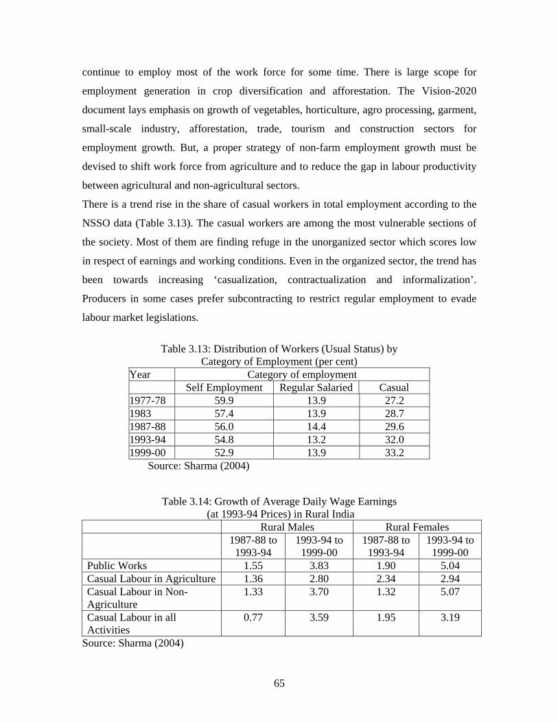
65

continue to employ most of the work force for some time. There is large scope for

employment generation in crop diversification and afforestation. The Vision-2020

document lays emphasis on growth of vegetables, horticulture, agro processing, garment,

small-scale industry, afforestation, trade, tourism and construction sectors for

employment growth. But, a proper strategy of non-farm employment growth must be

devised to shift work force from agriculture and to reduce the gap in labour productivity

between agricultural and non-agricultural sectors.

There is a trend rise in the share of casual workers in total employment according to the

NSSO data (Table 3.13). The casual workers are among the most vulnerable sections of

the society. Most of them are finding refuge in the unorganized sector which scores low

in respect of earnings and working conditions. Even in the organized sector, the trend has

been towards increasing ‘casualization, contractualization and informalization’.

Producers in some cases prefer subcontracting to restrict regular employment to evade

labour market legislations.

Table 3.13: Distribution of Workers (Usual Status) by

Category of Employment (per cent) Year Category of employment Self Employment Regular Salaried Casual 1977-78 59.9 13.9 27.2 1983 57.4 13.9 28.7 1987-88 56.0 14.4 29.6 1993-94 54.8 13.2 32.0 1999-00 52.9 13.9 33.2

Source: Sharma (2004)

Table 3.14: Growth of Average Daily Wage Earnings (at 1993-94 Prices) in Rural India

Rural Males Rural Females 1987-88 to

1993-94 1993-94 to

1999-00 1987-88 to

1993-94 1993-94 to

1999-00 Public Works 1.55 3.83 1.90 5.04 Casual Labour in Agriculture 1.36 2.80 2.34 2.94 Casual Labour in Non-Agriculture

1.33 3.70 1.32 5.07

Casual Labour in all Activities

0.77 3.59 1.95 3.19

Source: Sharma (2004)

66

While analyzing the National Council of Applied Economic Research survey results,

Shariff (1999) reports that labourers in rural India get 160 days of wage employment on

an average in a year. He notes: “Public policy should aim at improving entitlement

through creation of a larger number of employment days …Implementation of minimum

wages alone will not benefit wage workers” (P. 81). In this context, one positive feature

for the poor noted by Sharma (2004) and others is that real wage rate in various

categories of employment has risen considerably faster during 1993-99 than during 1987-

93 (Table 3.14). Radhakrishna and Rao (2006), too, provide evidence of acceleration in

real wage rate during the same period on the basis of NSSO data and note that the loss in

employment might have been compensated by rise in wages from the point of view of

total earnings by labourers. Based on information available in Agricultural Wages in

India, Deaton and Dreze (2002), however, report a deceleration in real wage rate from

about 5% per annum during 1980s to 2.5% during 1990s13. As examined in a later

chapter, a change in real wage rate has a strong influence on poverty.

Rise in real wage is the combined effect of several factors: agricultural productivity

growth, cropping intensity increase due to irrigation, expansion of non-farm activities and

large scale employment creation in public works programmes. Public works programmes

are supposed to adhere to minimum wage rates prescribed by the state governments and

are no longer negligible players in rural labour market. Evaluation studies do not always

find adherence to the minimum wages due to payment of piece wage, the explicit or

implicit wages in public works are closer to the prescribed minimum than agricultural

wages in the lean season14. The size of the public works programmes has grown to a

large extent over time and naturally put an upward pressure on agricultural wages. This

brings us to public provision of employment through direct programmes aimed at poverty

reduction.

13 So far as its impact on level of living of the poor is concerned, they note: “… even the reduced growth rate of agricultural wages in the nineties, at 2.5 per cent per year, points to significant growth in per capita expenditure among the poorer sections of the population”. 14 The legislation on minimum wage also applies to agriculture too, though its implementation becomes difficult in practice. Real wages are, however, not fixed in formal or informal sector due to changes in consumer prices. Revision of minimum wage takes place with lag of several years. Overall, however, real wage flexibility is limited to play a market-clearing role.

67

3.10 Public Employment Programmes Government of India has undertaken two types of programmes to directly enhance

income earning opportunities for the poor during the last three decades. These are: (a)

wage employment programmes, and (b) self-employment programmes. There have been

several programmes under each category targeted at specific groups15.

The Food for Work Programme started in mid-1970s to provide public works to the poor

by making use of a portion of the large stocks of foodgrains available with the

government due to its market intervention operations (discussed earlier in Box 3.1). A

good part of the wage was paid in kind in terms of foodgrains and hence the name ‘food

for work’. Various other wage employment programmes like the National Rural

Employment Programme, the Jawahar Rozgar Yojana, have been undertaken in later

years to provide the rural unemployed or underemployed poor with supplementary wage

employment particularly during the lean agricultural season through public works like

village roads, ponds, irrigation wells and school buildings in or around their village. Part

of the wages continue to be often paid in kind. The distinction of one programme from

the other could be in terms of coverage, mode of financing, sharing of responsibility

between the Central and state governments. Given the large overlapping nature of several

programmes, attempts have been made in recent years to merge them for administrative

and monitoring conveniences. The Sampoorna Grameen Rozgar Yojana (SGRY) and the

National Food for Work Programme are currently in operation and both are open to all

rural poor who are in need of wage employment and willing to carry out manual

unskilled work. The programmes normally target to cover a specified proportion of

beneficiaries from the scheduled tribe (ST) and scheduled caste (SC) groups as well as

from women. The size of these programmes has expanded substantially over the years.

SGRY-I & SGRY-II (two variants) together provided 748 and 764 million mandays of

15 Some of these programmes are named after one political leader or another.

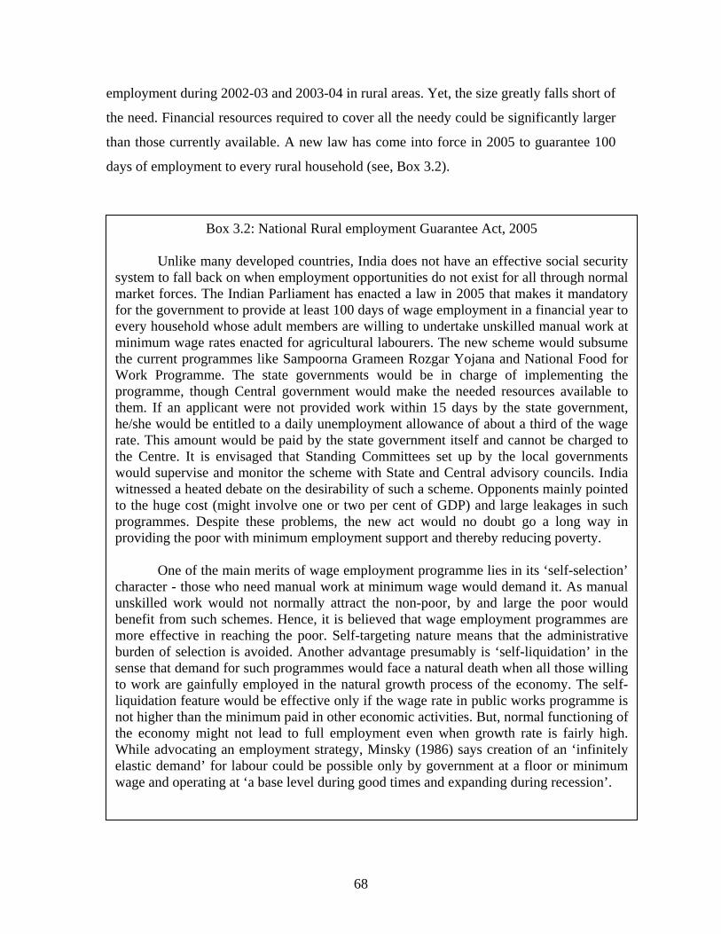
68

employment during 2002-03 and 2003-04 in rural areas. Yet, the size greatly falls short of

the need. Financial resources required to cover all the needy could be significantly larger

than those currently available. A new law has come into force in 2005 to guarantee 100

days of employment to every rural household (see, Box 3.2).

Box 3.2: National Rural employment Guarantee Act, 2005

Unlike many developed countries, India does not have an effective social security system to fall back on when employment opportunities do not exist for all through normal market forces. The Indian Parliament has enacted a law in 2005 that makes it mandatory for the government to provide at least 100 days of wage employment in a financial year to every household whose adult members are willing to undertake unskilled manual work at minimum wage rates enacted for agricultural labourers. The new scheme would subsume the current programmes like Sampoorna Grameen Rozgar Yojana and National Food for Work Programme. The state governments would be in charge of implementing the programme, though Central government would make the needed resources available to them. If an applicant were not provided work within 15 days by the state government, he/she would be entitled to a daily unemployment allowance of about a third of the wage rate. This amount would be paid by the state government itself and cannot be charged to the Centre. It is envisaged that Standing Committees set up by the local governments would supervise and monitor the scheme with State and Central advisory councils. India witnessed a heated debate on the desirability of such a scheme. Opponents mainly pointed to the huge cost (might involve one or two per cent of GDP) and large leakages in such programmes. Despite these problems, the new act would no doubt go a long way in providing the poor with minimum employment support and thereby reducing poverty.

One of the main merits of wage employment programme lies in its ‘self-selection’

character - those who need manual work at minimum wage would demand it. As manual unskilled work would not normally attract the non-poor, by and large the poor would benefit from such schemes. Hence, it is believed that wage employment programmes are more effective in reaching the poor. Self-targeting nature means that the administrative burden of selection is avoided. Another advantage presumably is ‘self-liquidation’ in the sense that demand for such programmes would face a natural death when all those willing to work are gainfully employed in the natural growth process of the economy. The self-liquidation feature would be effective only if the wage rate in public works programme is not higher than the minimum paid in other economic activities. But, normal functioning of the economy might not lead to full employment even when growth rate is fairly high. While advocating an employment strategy, Minsky (1986) says creation of an ‘infinitely elastic demand’ for labour could be possible only by government at a floor or minimum wage and operating at ‘a base level during good times and expanding during recession’.

69

Among the self-employed programmes, one programme that attracted the

attention of many observers of the poverty scene was the Integrated Rural Development

Programmes (IRDP) started in 1980 to enable poor households to cross over the poverty

line through self-employment. The government played a role in the direct provision of

productive assets and inputs or financial assistance for their procurement with a major

subsidy component. The activities under IRDP were initially mostly in the primary sector

like irrigation or animal husbandry, but extended later to several areas like weaving, food

processing, trade and other services.

IRDP has been redesigned and renamed as Swarnajayanti Gram Swarojagar Yojana

(SGSY). It encourages the poor potential beneficiaries to be organized as micro

enterprises called Self Help Groups (SHGs)16 who receive group bank credit and

government subsidy. The SHGs in turn lend to individual members or undertake some

group activities. Peer group pressure works for repayment of loan even in the absence of

collaterals. During 2002-03 and 2003-04, about one million beneficiaries have received

assistance under SGSY per year.

Targeting in poverty reduction programmes is not perfect and many non-poor households

get selected. Even after allowing for leakages, these schemes have significantly

contributed to the upliftment of rural poor households. Proper identification of viable

projects could contribute to the success of poverty reduction through self-employment.

Marketing support for their produce is another area where the poor need help from

agencies in nearby urban centres. Local governments in both rural and urban areas are in

positions to take into consideration the local needs and local resource availability.

Involvement of local government in the design and monitoring of projects have generally

been found to be more fruitful. Public-private partnership through involvement of the

non-government organizations (NGOs) with good track record has also contributed to

viability of self-employment programmes.

In urban areas too, there are special schemes for the poor for wage employment and self-

employment in micro enterprises. Training and skill creation for the unemployed persons

to enable them for self-employment has been another major component of urban poverty

reduction schemes. Similarly, some programmes aim at facilitating construction of

16 Many non-governmental organizations have also been active participants in the SHG initiatives.

70

dwelling units for rural and urban poor and improvement of sanitation and environment.

There are also area development programmes in operation for deserts and drought prone

areas meant to help the naturally disadvantaged areas. Although the focus in some of

these programmes is not directly the poor as such, their target groups comprise bulk of

the poor.

3.11 Impact of Privatisation17

Restructuring of public enterprises, including privatization, has been an important

component of the economic reform process in India. Over the years, 242 Central Public

Enterprises (CPEs) and 1068 State Level Public Enterprises (SLPEs) have involved an

investment of about Rs 7,10,000 crore. They provide employment to about 4 million

people. The accumulated losses of these enterprises are approximately Rs 97,000 crore.

The net worth of the CPEs has been estimated to be Rs 2,41,846 crore and that of SLPEs

Rs 44,631 crore.

The impact of privatization on incidence of poverty is not a straight forward one. Private

firms are basically motivated by profit maximization. Privatization could reduce poverty

if it contributes to economic growth without major adverse effect on distribution. But, as

Bayliss (2002) notes the positive impact of privatization on growth has not yet been

empirically established. Low income groups, either as consumers or producers, may also

benefit from privatization or restructuring process if services provided by the public

sector utilities are made available in a reliable manner and at affordable rates. Entry of

private players in Indian telecom sector has increased access to its services, offered a

variety of products, registered sharp decline in tariff charged to consumers, and improved

customer relationship. On the other hand, power sector reforms in India have not led to

perceptible increase in competition and consumers have not benefited from service.

Privatization has attracted opposition mainly due to the fear that it would lead to

reduction in employment through large scale retrenchment of workers18. Table 3.15

reveals that the aggregate employment declined by as much as 48 per cent in the SLPEs.

17 This section is based on the background paper “Privatisation Policy” by R.K. Mishra. 18 Another criticism of the privatization process is that public assets are being sold for a song in some instances.

71

Andhra Pradesh, Delhi, Haryana, Gujarat, Karnataka, Orissa, Punjab and Rajasthan

contributed a major share to this decline. The labour force in these states comprised not

only permanent labour but also ad hoc and muster roll labour. Most states did not follow

the concept of manpower planning and therefore the actual labour force exceeded the

‘sanctioned strength’.

Table 3.15: Aggregate Employment Trends in State Public Enterprises

States 97-98 98-99 1999-00 2000-01 2001-02 2002-

03 2003-04Andhra Pradesh 351928 350465 345938 332551 303806 287276Assam 57024 55933 55297 - - - -Delhi - - - - 58550 50070 45347Gujarat 142399 139685 138675 137860 Haryana 53762 51995 42678Karnataka 172309 162710 168256 156255 Kerala 120687 125814 128021 124661 Maharashtra 296331 241040 243561 Orissa 40878 20460 Punjab 118624 104519 100478Rajasthan 92255 85109 69976 67783Tamil Nadu 169000 16900 167646 167576 247708 Total 1046592 849094 1094891 1167689 1000101 739868 543562

Source: CAG Reports and BPE Reports of the concerned states.

Reduction in employment in case of CPEs has not been as large as in that in SLPEs, as

Table 3.16 reveals. Employment in disinvested CPEs as a proportion of total CPE

employment has remained nearly constant after the reforms. Thus, employment reduction

has taken place even in enterprises that were not subject to disinvestments. But, the

growth in employment in CPEs noticed prior to the reforms has been halted after the

reforms.

72

Table 3.16: Employment in Disinvested and Non Disinvested CPEs

Year Employment in all 240 CPEs

Employment in CPEs that were Disinvested in 1991 and later

Employment in CPEs where disinvestment did not occur until 2001

Employment in Disinvested CPEs as percent of total CPE employment

1981-82 1940000 501258 1438742 25.841982-83 2020000 525569 1494431 26.021983-84 2070000 540738 1529262 26.121984-85 2110000 554359 1555641 26.271985-86 2150000 565804 1584198 26.321986-87 2210000 582571 1627429 26.351987-88 2210000 583006 1626994 26.381988-89 2210000 588385 1621615 26.621989-90 2240000 588797 1651203 26.291990-91 2220000 590595 1629405 26.601991-92 2180000 588830 1591170 27.011992-93 2150000 586313 1563687 27.271993-94 2070000 572158 1498742 27.641994-95 2060000 561989 1498011 27.281995-96 2050000 552611 1497389 26.961996-97 2010000 541825 1468175 26.961997-98 1960000 530373 1429627 27.061998-99 1900000 519668 1380332 27.351999-00 1850000 496651 1353349 26.85 Source: Department of Public Enterprises, Government of India, New Delhi, Public Enterprise Survey: Vol. 1,1981-82 to 2000-01

In order to minimize the adverse employment impact of privatisation, the government has

formulated a social safety net programme (SSNP). The SSNP includes retrenchment or

voluntary retirement benefits, and a rehabilitation component that aims at helping the

affected employees to acquire necessary skills to start new vocations. The employees are

provided with psychological counseling, if needed, to absorb the trauma of loss of

assured livelihood and to face the new challenges. The training agencies and the

concerned public enterprises also sponsor the applications of the affected employees

seeking financial assistance to commercial banks. State governments have often faced

problems in providing SSNP with adequate funding. A portion of disinvestments

proceeds may be allocated to a national rehabilitation fund to ensure adequate safety net

mechanism so that workers losing jobs do not fall back into poverty.

73

3.12 Conclusion

National income growth in India was low at about 3.5 per cent per year for about three

decades till late 1970s. Economic growth picked up to above 5 per cent in 1980s

following an expansionary fiscal policy and a moderate dose of liberalisation. The market

friendly trade and industrial reforms started since 1991 helped the growth rate to pick up

further to about 6 per cent per annum.

Structure of GDP has changed substantially towards industry and services over the

decades. Agriculture has lost its dominant position and accounted for about a fifth of

GDP in 2005. Yet, as much as 60 per cent of the work force still depends on agriculture

as a major source of earning. Consequently, labour productivity in agriculture is about a

forth of that in non-agriculture. The success of the green revolution in parts of the country

helped not only in achieving self sufficiency in food grain production but also in building

up of huge stocks in government warehouses. The industrial growth process has been

more evenly dispersed across use-based sectors after liberalisation. But, contrary to

earlier expectations, a big jump in share of unregistered manufacturing has not been

evident after the reforms. The recent growth in India has been mostly driven by the

service sector which now accounts for 52 per cent of GDP.

Stagnation in agricultural growth in recent years has been a major cause of concern from

the point of view poverty reduction. A higher agricultural growth would be needed for

faster poverty reduction. While Indian economy did benefit from total factor productivity

growth in earlier periods, evidence of its occurrence after the reform is at best mixed.

Income elasticity of employment has fallen during the 1990s and proportion of casual

labour has increased. The social safety net programme may be strengthened to ensure that

workers losing jobs do not fall back to poverty. Rise in real wages has been a positive

feature of the labour market. Government has undertaken several wage employment and

self employment programmes to supplement the income earning opportunities for the

poor. The new act guaranteeing 100 days of wage employment to every rural household

in a year is a welcome move and, when implemented fully, could significantly contribute

to poverty reduction.

74

75

Chapter 4

Fiscal Developments19 4.1 Introduction Fiscal policy is a major instrument of government intervention for poverty reduction.

Successive governments in independent India have regarded improvement in the living

condition of the poor as one of the major objectives of their fiscal policy. Governments

have recognized their direct responsibility in provision of basic needs of life like

nutrition, health, sanitation and education along with provision of employment for

livelihood of the poor as discussed in the last chapter. These interventions are not

undertaken simply as a means to achieve other social objectives, but have been viewed as

ends in themselves. The logic of intervention thus goes beyond the externality argument

of fiscal intervention for poverty reduction. Sensitivity to the conditions of the poor

obviously matters in a democratic setup of government where every citizen has one vote.

Yet, governments in a developing country like India face many problems - some of which

are their own making while others are external - in reorienting government expenditure

leading to a wide gap between promises and practice. Overall, India has been successful

in avoiding famines involving large-scale deaths but not persistent under-nutrition,

moderate hunger and even starvation deaths in some regions.

4.2 Trends in Major Budgetary Parameters Table 4.1 shows the trends in major fiscal parameters of the central government since

1990-91. The total expenditure of the central government as a proportion of GDP fell by

2 percentage points in the post-reform years indicating lower level of government

activity. The 1991 reform package undertaken by India envisaged reduction in fiscal

deficit to sustainable level for ensuring macroeconomic stability and fiscal correction

measures received overriding priority over other considerations. Thus, the fall in

government total expenditure relative to GDP was in line with the stabilisation objective.

But, concern had been expressed in several quarters on the composition of expenditure.

Capital expenditure of government dropped after 1991 and remained lower by about 2%

19 This chapter is written by Manoj Panda and Seeta Prabhu.

76

of GDP for about a decade. It has partially recovered since 2001. Share of public sector in

total capital formation in the economy dropped from about 45% prior to reforms to less

than 25% in 2002-03 (Figure 4.1). There is a need for a rethinking on this trend

particularly in view of the infrastructure development needs in backward regions in East

and Central India that now contain most of poor. Public sector investment in

infrastructure and social services plays a critical complementary role to attracting private

investment apart from inducing private investment through demand generating multiplier

process.

Table 4.1: Receipts and Expenditure of Central Government (As percent of GDP)

1990-91 1999-00 2000-01 2001-02 2002-03 2003-04 2004-051

Revenue receipts (net) 9.7 9.4 9.2 8.9 9.4 9.6 9.8Tax revenue (Net of State Shares) 7.6 6.6 6.5 5.9 6.5 6.8 7.2Non-tax revenue 2.1 2.7 2.7 3.0 2.9 2.8 2.6Revenue expenditure 12.9 12.9 13.3 13.3 13.8 13.1 12.3Revenue deficit 3.3 3.5 4.1 4.4 4.4 3.6 2.5Capital receipts 5.6 6.0 6.4 7.1 7.4 7.5 6.2Capital expenditure 4.4 2.5 2.3 2.7 3.0 4.0 3.6Total expenditure 17.3 15.4 15.6 15.9 16.8 17.1 16.0Fiscal deficit 6.6 5.4 5.7 6.2 5.9 4.5 4.1Primary deficit 2.8 0.7 0.9 1.5 1.1 0.0 0.0Sources of Tax Revenue Direct 1.9 3.0 3.3 3.0 3.4 3.8 4.2 Personal income tax 0.9 1.3 1.5 1.4 1.5 1.5 1.5 Corporation tax 0.9 1.6 1.7 1.6 1.9 2.3 2.7Indirect 7.9 5.8 5.7 5.1 5.3 5.3 5.5 Customs 3.6 2.5 2.3 1.8 1.8 1.8 1.8 Excise 4.3 3.2 3.3 3.2 3.3 3.3 3.2 Service tax 0.0 0.1 0.1 0.1 0.2 0.3 0.5Total 10.1 8.9 9.0 8.2 8.8 9.2 9.8

Note: 1 Provisional Source: Economic Survey 2005-2006, Government of India

Central government total expenditure has picked up in recent years and has remained in

the range of 16-17% of GDP. Revenue expenditure has increased faster than GDP partly

due to substantial increase in salary and pension for government servants since mid-

1990s. The consequent rise in revenue deficit implied that the government borrowed for

77

meeting its current expenditure and not for productive investment that could generate

capacity to repay the loan. According to Acharya (2001), effects of the Fifth Pay

Commission for government employees constituted ‘the single largest adverse shock’ to

public finance in the 1990s and led to an up-turn in fiscal deficit in 1996-97. His

estimates indicate that compensation to employees (including pension) by Central and

State governments accounted for about half of the fiscal deficit increase of 3 percentage

points of GDP during 1996-1999.

15.020.025.030.035.040.045.050.055.0

1950

-51

1953

-54

1956

-57

1959

-60

1962

-63

1965

-66

1968

-69

1971

-72

1974

-75

1977

-78

1980

-81

1983

-84

1986

-87

1989

-90

1992

-93

1995

-96

1998

-99

2001

-02

% Share of Public Sector in GDCF

Figure 4.1: Share of Public sector in Gross Domestic Capital Formation

Interest payments, which stood at 4.1 per cent of GDP in 2004-05, continue to be the

largest single item of Central government expenditure because of high debt burden of the

past. Fiscal deficit level dropped after 1991, but picked up during mid-1990s. Fiscal

deficit of Center and State governments together stood close to 10 per cent of GDP in

2003-04 and constitutes a major slippage of the reform process. The Central government

has succeeded in eliminating primary deficit since 2003-04. Primary deficit is calculated

as fiscal deficit net of interest payments and reflects government’s efforts in managing

relatively non-committed expenditure compared to its revenue. While several measures

were undertaken over the years to improve the fiscal health of the economy, a lot yet

remains to be done. A noteworthy recent development has been the passage of the Fiscal

Responsibility and Budget Management (FRBM) Act 2003, which stipulates that fiscal

78

deficit and revenue deficit must be corrected as per laid down rules. This is expected to

reduce the interest burden to moderate level in future.

Total tax revenue as a proportion of GDP fell during 1990s but has displayed an upward

trend in recent years. The fall in tax revenue seems to be an inevitable medium run cost

of customs duty reduction and rationalization of customs and excise as part of the reform

process. Tax burden on the manufacturing sector was disproportionately large compared

to its share in GDP. Agriculture is in the state list and is virtually exempted from income

tax. The service sector was not in the tax network till 1993-94, though it was fast growing

and its contribution to the national income growth was maximum. Attempts have been

made to widen the tax base with the introduction of the service tax and to extend its

coverage gradually. An important development on the revenue side has been that direct

taxes currently contribute to about 45% of Central tax revenue as against 20% in 1990-

91. This compositional change in tax structure is certainly in the right direction as direct

taxes are generally regarded as progressive and less distortionary in their impact than

indirect taxes.

In several respects, state governments in India together play as important role as the

Central government. Their total expenditure currently amounts to 19 per cent of GDP

(Table 4.2). Capital expenditure of state governments dropped during the reform period.

Ability of the state governments to intervene on poverty related programmes gets dictated

by their fiscal health. Pay revision in late-1990s created more fiscal stress for state

governments as revealed by rise in revenue deficit from 0.9 per cent of GDP in 1990-91

to 2.5 per cent in 2000-01. The extent of the stress on state budgets could be judged from

the fact that salary and pensions take away 80-90 per cent of revenue receipts by most of

the states since mid-1990s. They are not in a position to pay their matching shares of 10-

30 per cent in several centrally sponsored development schemes (see, Box 4.1). A major

development at the state level is the adoption of value added tax (VAT) by most states

from 2005-06. A two-tier VAT has been adopted for almost all goods: 4% for basic

necessities and 12.5% for others except for a few goods. The Central sales tax would also

be phased out. The VAT would help to remove cascading tax burden. Tax revenue is

expected to rise as compliance improves under VAT.

79

Table 4.2: Receipts and Disbursements of State Governments (As percent of GDP)

1990-91 2000-01 2001-02 2002-03 2003-04 2004-051

Total receipts 16.0 16.6 16.4 17.4 19.1 18.9 Revenue receipts 11.7 11.3 11.2 11.4 11.5 12.3

Tax receipts (including share in Central pool)

7.8 8.0 7.9 8.1 8.2 8.6

State's own tax revenue 5.3 5.6 5.6 5.8 5.8 6.0 Non-tax receipts 3.8 3.3 3.3 3.3 3.2 3.7

Total disbursements 16.0 16.5 16.5 17.2 19.1 19.0 -Revenue 12.6 13.8 13.8 13.7 13.7 13.7 -Capital 2.4 2.1 2.2 2.9 4.4 4.6

Revenue deficit 0.9 2.5 2.6 2.2 2.2 1.4 Gross fiscal deficit 3.3 4.2 4.2 4.2 4.5 4.0 Source: Economic Survey 2005-06, Govt. of India. 1 Revised estimate (RE)

The states receive about 30 per cent of total tax collection by the Centre from the

shareable common pool. The Central government decides allocation of fiscal transfers to

State governments mostly on the basis of recommendations of the Finance Commission

set up at intervals of five years and the Planning Commission, a permanent body. Fiscal

transfers are in principle guided by equity considerations along with other factors and

states with larger proportion of poor population generally receive higher per capita

transfers within comparable categories20. Such transfers in totality add to general

resources of the states and portions received on poverty considerations are neither

separately shown nor earmarked for poverty reduction programmes. Thus, while fiscal

transfers help to raise the overall resource position of poorer states to spend more on

poverty reduction programmes, it does not ensure that intra-state allocation of resources

is in favour of poorer regions or poorer population. Intra-state allocation is at the

discretion of state government and not based on clearly defined principles.

20 Some border states enjoy special category status and receive larger transfers.

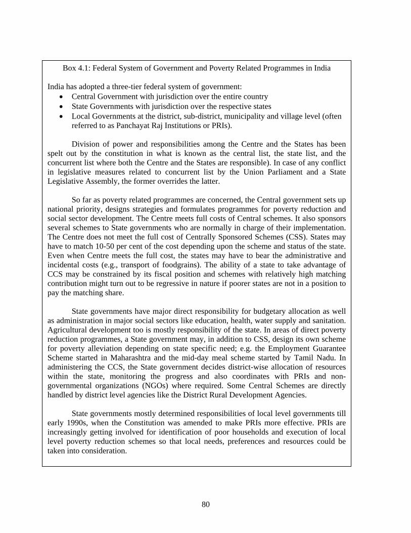
80

Box 4.1: Federal System of Government and Poverty Related Programmes in India India has adopted a three-tier federal system of government:

• Central Government with jurisdiction over the entire country • State Governments with jurisdiction over the respective states • Local Governments at the district, sub-district, municipality and village level (often

referred to as Panchayat Raj Institutions or PRIs).

Division of power and responsibilities among the Centre and the States has been spelt out by the constitution in what is known as the central list, the state list, and the concurrent list where both the Centre and the States are responsible). In case of any conflict in legislative measures related to concurrent list by the Union Parliament and a State Legislative Assembly, the former overrides the latter.

So far as poverty related programmes are concerned, the Central government sets up

national priority, designs strategies and formulates programmes for poverty reduction and social sector development. The Centre meets full costs of Central schemes. It also sponsors several schemes to State governments who are normally in charge of their implementation. The Centre does not meet the full cost of Centrally Sponsored Schemes (CSS). States may have to match 10-50 per cent of the cost depending upon the scheme and status of the state. Even when Centre meets the full cost, the states may have to bear the administrative and incidental costs (e.g., transport of foodgrains). The ability of a state to take advantage of CCS may be constrained by its fiscal position and schemes with relatively high matching contribution might turn out to be regressive in nature if poorer states are not in a position to pay the matching share.

State governments have major direct responsibility for budgetary allocation as well

as administration in major social sectors like education, health, water supply and sanitation. Agricultural development too is mostly responsibility of the state. In areas of direct poverty reduction programmes, a State government may, in addition to CSS, design its own scheme for poverty alleviation depending on state specific need; e.g. the Employment Guarantee Scheme started in Maharashtra and the mid-day meal scheme started by Tamil Nadu. In administering the CCS, the State government decides district-wise allocation of resources within the state, monitoring the progress and also coordinates with PRIs and non-governmental organizations (NGOs) where required. Some Central Schemes are directly handled by district level agencies like the District Rural Development Agencies.

State governments mostly determined responsibilities of local level governments till

early 1990s, when the Constitution was amended to make PRIs more effective. PRIs are increasingly getting involved for identification of poor households and execution of local level poverty reduction schemes so that local needs, preferences and resources could be taken into consideration.

81

The combined budgetary position of Central and state governments is given in

Table 4.3 after taking into account inter-governmental transfers. Total government

disbursement of funds was 29 per cent of GDP in 2004-05. Total tax revenue by Centre

and states was 15.8 per cent of GDP and non-tax revenue another 4.2 per cent. Revenue

deficit and gross fiscal deficit stood at 4.1 and 8.4 per cent of GDP in 2004-05.

Table 4.3: Combined Budget of Central and State Governments (As percent of GDP)

1990-91 2000-01 2001-02 2002-03 2003-04 2004-051

Total disbursements 28.7 28.1 28.3 28.8 28.9 29.0 Total receipts 26.7 28.2 28.2 28.9 29.0 28.1

Revenue receipts 18.6 18.0 17.5 18.5 18.8 20.0 Tax receipts 15.4 14.5 13.8 14.6 15.0 15.8

Revenue deficit 4.2 6.6 7.0 6.7 5.8 4.1 Gross fiscal deficit 9.4 9.5 9.9 9.6 8.5 8.4

Source: Economic Survey 2005-2006, Government of India. 1. Revised estimate (RE)

4.3 Fiscal Policy and the Poor Fiscal policy affects the poor through several channels. Fiscal stability is an important

component of overall macroeconomic stability. Large fiscal deficit might spill over into

balance of payments deficit and precipitate the risk of an external crisis, as it is believed

in some quarters to have happened during the 1980s. The poor are hard hit by the

stabilization programmes when a crisis occurs. The current fiscal deficit level in India is

almost similar to the level that prevailed during the 1991 crisis, yet it has not got

precipitated in an external crisis. Ahluwalia (2002) explains that this is due to a

neutralizing shrinkage in demand effect from the private sector, which witnessed only a

marginal rise in investment-GDP ratio while savings of the private sector rose

substantially by 4-5 percentage points of GDP during 1990s.

Government allocates a good proportion of its budgetary resources for traditional public

services like security, law and order, justice, general administration that are in principle

82

available to all citizens at the time of need either free of cost or at nominal charge21. The

poor, however, may not be able to make use of many of these services to the same extent

as the rich since access to public services involve private costs22 like traveling to nearby

town and foregoing earnings which the poor cannot afford easily. Moreover, there is also

an issue of sensitizing the bureaucracy to provide the haves and the have-nots with equal

attention. The latter might have to pay several visits for services that the former can avail

in one or two visits, at times with payment of quick or convenience money. If private

access costs for government services could be made affordable to the poor, they could

benefit more from various government services.

Next, fiscal policy influences overall growth that in turn affects all sections of the

population including the poor. Restructuring of government expenditure in favour of

physical and social infrastructure is critical for long-term growth, while Keynesian

demand generation could help short-term growth if there is excess capacity. Public

provision of infrastructure could increase the prospects for attracting private investment

and play a crowding in role. Large volume of committed expenditure such as interest and

pension payments often constraints the ability of the government to support growth.

Volume of the rest of expenditure, classified in budget as primary expenditure, does not

necessarily indicate capability of the government to support growth. State governments in

India currently spend as much as 80-90 per cent of their plan expenditure to meet salary

bill and are left with very limited flexibility to undertake new programmes on their own.

In this sense government salary bill is also a quasi-committed expenditure, though some

of the employees could be redeployed to new activities.

Fiscal restructuring is needed to expand efficient provision of infrastructure services for

higher growth. The effectiveness of the growth channel on poverty reduction would be

largely determined by distributional factors including demand for unskilled or semi-

skilled employment. As discussed in the previous chapter, India’s recent track record on

employment front has not been particularly encouraging. From poverty reduction point of

view, regional distribution of infrastructure investment has emerged as an important

21 Budgetary allocation in the year 2003-04 for administrative service was of the order of Rs. 446 billion and another Rs. 55 billion under the head organs of the state. Together they accounted for 1.8 per cent of GDP. Defence services accounted for another 2.3 per cent of GDP. 22 See, Srivastava et. al, 2004.

83

dimension in India with concentration of poor in Eastern and Central India in recent

years. The Centre needs to intervene more directly for infrastructure development of this

region.

4.4 Social Sector Expenditure One area of budgetary allocation that plays a crucial role for welfare of the poor is the so-

called social sector expenditure that enhances opportunities for human development and

helps poverty alleviation in the long run. Based on budgetary classification of

government expenditure, it is a normal practice to consider social sector expenditure as

sum of expenditure under heads Social Services and Rural Development; the former

includes health, education, family welfare, water supply, nutrition and sanitation and the

latter includes directly targeted poverty reduction programmes like employment

generation programmes discussed in the previous chapter. While Central government is

involved in designing and making financial provision for Centrally Sponsored Schemes

(CSS), the states play the important role in execution apart from having their own

programmes (see, Box 4.1).

Table 4.4 gives expenditure on social sectors by Centre and State governments. Social

sector expenditure accounts for 6-7 per cent of GDP and about a quarter of total

government expenditure. As a percentage of GDP, social sector expenditure fell during

the post reform period. It was the highest in 1989-90 at 7.2 per cent which has not been

recovered till 2003-04, though 2002-03 value was very close to that in 1989-90. As a

proportion of total government expenditure, social sector expenditure fell during first half

of 1990s, recovered during second half but has fallen again since 2000-01. Social sector

expenditure in real per capita terms fell for three years after the reforms, but has been on

a rising trend since mid-1990s. On this count at least, government has not been

insensitive to social sector issues, although social sector expenditure has not always been

keeping pace with changes in GDP or total government expenditure.

Expenditure on rural development component, which includes poverty reduction

programmes, is close to 1 per cent of GDP. Efficacy of these programmes has varied

depending on types of programmes and regions. Leakage of the benefits in case of

targeted poverty reduction programmes to the non-target group is a major problem.

84

Overall, income benefits to the poor seem to be more in employment programmes

relative to other programmes. Mid-day meal schemes in schools as well as special

nutrition programmes for women and children (Anganwadi) have been found to be

successful in many parts of the country. Sen (1996) makes a very persuasive argument to

include government development expenditure variable in equations determining poverty

over time. He finds per capita real development expenditure to have a significant poverty

reducing effect.

Table 4.4: Social Sector Expenditure by Central and State Governments

Year As % of GDP As % of total govt. expenditure

Per capita expenditure (in Rs) in 1993-94 prices

1987-88 7.26 25.29 564 1988-89 6.95 25.22 585 1989-90 7.17 25.19 635 1990-91 6.78 24.85 623 1991-92 6.58 24.28 599 1992-93 6.38 24.06 594 1993-94 6.46 24.58 622 1994-95 6.39 25.01 632 1995-96 6.40 25.95 674 1996-97 6.30 26.46 716 1997-98 6.41 26.18 763 1998-99 6.80 26.54 856 1999-2000 6.93 25.96 923 2000-01 6.56 24.83 790 2001-02 6.30 23.42 859 2002-03 7.11 24.78 995 2003-04 6.82 24.36 998 Note: Social sector includes Social Services and Rural Development on both revenue and capital accounts. Source: Dev and Mooij (2005) till 1997-98. Data from 1998-99 based on Indian Public Finance Statistics, Ministry of Finance, GOI, 2004

Srivatsava et. al (2004) draw attention to several drawbacks of the Centrally Sponsored

Schemes like absence of consultation with states while formulating them, arbitrary

allocation across states and inability of states with financial problems to pay matching

contribution. They find that pattern of grant for Central and Centrally Sponsored

Schemes does not have any bearing on either poverty or per capita income of the states.

In per capita terms on an average during 1999-00 and 2000-01, it was as low as Rs. 46

85

and Rs. 57 for poor states like Uttar Pradesh and Bihar respectively compared to Rs.151

for Goa, which is the richest state and Rs. 136 for Karnataka in the middle rung.

Rajashthan, which is emerging out of poverty, was among the highest recipients of the

grant through out 1990s.

4.5 Subsidies Central and State governments undertake large scale subsidization of several goods and

services in India, the stated objective often being extending a helping hand to the poor

and other vulnerable groups in the society. Explicit government budgetary subsidy like

those on food, fertilisers and petroleum products is only a small portion of total subsidy.

Several subsidies get hidden in the production of intermediate goods and services and

quantum of subsidy at the stage of final consumption of goods or service is not clearly

known. This creates difficulties in identification of income status of beneficiaries. As

Srivastava et. al (2004) maintains extent of benefits derived by different income groups

from such subsidies is likely to be broadly in proportion to the final expenditure made on

the subsidized items and as such the poor might derive a proportionately small benefit

from non-targeted subsidies.

According to ‘Economic Survey 2004-05’, explicit and implicit subsidies by Central

government are of the order of about Rs. 116,000 crores in 2003-04 or 4.2 per cent of

GDP. About 42 per cent of this falls in the merit category and the rest in non-merit

category. There is general agreement on the need to be revised upwards to reduce

subsidies, specially of the non-merit type. However, the division of merit and non-merit

goods is not always based on objectivity. For example, classification of higher education

into non-merit good could attract criticism on the grounds that abolition or near abolition

of subsidy from higher education could result in the rich having exclusive access to

higher education, which would not only accentuate future income distribution but could

compromise long run efficiency too as the potentially best might be left out of higher

education.

Volume of food subsidy jumped from Rs. 2450 crores in 1990-91 to Rs. 25800 crores in

2004-05 (as a percentage of GDP, food subsidy rose from 0.4 in 1990-91 to 0.8 in 2004-

05), partly due to enhanced food security measures with higher subsidy rate for the poor.

86

But, part of the subsidy volume rise is due to high minimum support price for foodgrain

procurement and inefficient operationd of Food Corporation of India. It indicates scope

for subsidy reduction without hurting the poor. Government has taken some measures

recently to make food subsidy more target group oriented by overhauling the public

distribution system and introducing differential prices for destitute, poor and non-poor

groups.

Several studies have attempted to make a comprehensive estimate of implicit and explicit

subsidies by Central and state governments and the estimated figures are much higher at

about 12-13.5 per cent of GDP23 during late 1980s and 1990s (e.g., Mundle and Rao,

1992 and NIPFP, 1997). Sustenance of such high subsidies is not feasible particularly

when fiscal deficit levels are high. Some types of subsidies, are of course, justified on

grounds of equity among present generation as well as of inter-generational equity (if

they help future growth through physical and social capital formation). One problem

noted by Srivastava et. al (2004) is that incidence of subsidy cannot be controlled for

most of the subsidies when these are input based like those in irrigation, power,

manufacturing and transport. In case of subsidized final goods like food subsidy,

targeting is possible but poorly administered. Following the dismantling of

Administrative Price Mechanism in petroleum products, petroleum subsidies are directly

borne by the budget since 2002-03. These have been regarded as non-transparent and

regressive in impact.

4.6 State Finance and Social Sector Expenditure The period of economic reforms has imposed considerable strain on the resources of

State governments (Table 4.5 and 4.6). The State governments incur bulk of the spending

on social sectors and hence their fiscal health has a direct bearing on the spending on

social sectors. While attempting to correct its own fiscal deficit, Central government

reduced its grants to the states particularly during the second half of 1990s when Centre’s

contribution in total revenue receipts of the states fell to 14-16% from 18-20% during

early 1990s. Tax revenue of states as a proportion of their revenue receipts, an indicator

23 Figures taken from Srivastava et. al (2004) based on revised GDP series and might differ from original estimates in the studies.

87

of tax efforts of States, moved up slightly from 66-69 per cent in pre 1991 years to 69-73

per cent between 1998-98 to 2003-04 due to a rise in the States’ own tax revenue. Tax

revenue of the states as a proportion of GDP has moved between 8 and 9 per cent without

showing any improvement. State governments had to face the burden of salary and

pension revision with much difficulty and it has got reflected in plan and development

expenditure. Resort to market borrowing contributed to rising interest payments.

Local bodies are expected to carry out several important functions. While the institutions

to ensure transfer of resources from the Centre to the States are well established, a similar

institutional set-up to ensure transfer of resources from the State government to the local

bodies is yet to gather strength. Decentralisation contributes to deepening of democracy

by enabling people to participate in the democratic process. In India, the impetus that

decentralization received through the 73rd and 74th Constitutional amendments,

particularly the one-third representation given to women has been widely commended

(UNDP, 2002).

Real per capita expenditures on social services as well as on items of social priority such

as elementary education, rural health, public health water supply, sanitation and nutrition

have been shown in Table 4.7. At the level of 15 major States level there has been an

increase of around 36 per cent between 1988-89 to 1990-91 (period 1) and 1999-00 to

2001-02 (period 2). When rural development expenditures are included, the increase is

somewhat lower at 31 per cent. As is to be expected, there are large variations across

States. The three low income low human development States of Bihar, Madhya Pradesh

and Uttar Pradesh have experienced a decline in real per capita expenditures ranging

between 14 and 24 per cent for social services expenditure and between 17 and 24 per

cent for social priority expenditure. In the case of social services and rural development

taken together, the decline was of a slightly higher magnitude ranging between 17 and 26

per cent.

The highest increase in per capita expenditure was experienced by Gujarat for social

services including for the combined expenditure on rural development. Maharashtra

recorded the highest increase of about 75 per cent in terms of social priority expenditures

which was higher than the 61 per cent increase in expenditure on social services

indicating a reorientation towards primary level services. Karnataka and West Bengal

88

among the middle income states fare relatively better in terms of social services recording

increases of over 70 per cent in real per capita terms, whereas in social priority,

Karnataka and Andhra Pradesh recorded increases of a similar magnitude. Karnataka and

West Bengal also fared better in terms of the combined social services and rural

development expenditure recording over 60 per cent increase between the two time

periods. Among the low income States, the performance of Orissa and Rajasthan was

relatively better with respect to all three categories of expenditure with increases ranging

between 39 to 55 per cent over the period under consideration.

The social allocation ratio (SAR), which expresses expenditure on social services as a

proportion of total expenditure, indicates a decline of about 5 per cent for 15 major states

(Table 4.8). As many as 9 states recorded a decline in the SAR and included low income

low human development states such as Uttar Pradesh and Bihar as well as high income

states such as Punjab and Haryana and middle income states like Andhra Pradesh and

West Bengal. Maharashtra recorded the highest increase in the SAR over the two time

periods.

Social priority ratio (SPR), which is the ratio of expenditure on social priority items

(listed above) in total social services expenditure, indicates the reorientation towards

social priority concerns has also been limited with the ratio remaining virtually stagnant

at the level of 15 major States. Seven states recorded decline in the ratio ranging between

5 and 18 per cent. Haryana recorded the highest increase, though the state had a decline

in the SAR of about 7 per cent. A similar situation is observed with respect to Andhra

Pradesh.

As a result, the human expenditure ratio (HER), which is the ratio of social priority

expenditures to GSDP, recorded a marginal decline at the level of 15 major States and

sharp declines with respect to many States. Declines were particularly sharp in Goa,

Punjab, Tamil Nadu and West Bengal. Haryana, Orissa, Maharahstra, Andhra Pradesh

and Rajasthan recorded substantial increases in HER ranging between 15 to 21 per cent.

Even when rural development expenditures are included with social services and

expressed as a proportion of GSDP, the situation is not very different. As many as ten

States recorded declines in the ratio with Gujarat, Madhya Pradesh and Orissa recording

increases ranging between 9 and 19 per cent.

89

Our focus is on human development for two reasons. The first is that the status of human

development needs substantial improvement if the goals of Education for All (adopted in

the National Policy on Education in 1986 and reiterated in the revised policy in 1992),

and the goal of Health for All (adopted in the National Health Policy of 1983 and

reiterated in the revised policy in 2001) and which were to be achieved by 1990 continue

to be elusive. The second is that the process of economic reforms adopted by several

State governments in the recent past could release resources as the State withdraws from

sectors in which it is no longer required to be present and begin to focus on social sectors

which are now considered a greater priority for State intervention. This provides an

opportunity to adopt innovative strategies for financing of social sectors now than in the

past.

Table 4.5: Pattern of Revenue Receipts of State Governments: 1988-89 to 2003-04 (in per cent)

Years Tax rev/ Revenue receipts

States own tax/ revenue receipts

States own non tax/ revenue receipts

Share in central tax/ revenue receipts

Grants from center / revenue receipts

Total tax revenue/ GDP

Loans from centre/ capital receipts

1988-89 65.72 44.44 15.12 21.29 19.16 8.76 58.271989-90 69.15 46.25 15.81 23.17 14.78 8.92 55.981990-91 67.08 45.65 13.9 21.43 18.68 8.73 56.241991-92 65.32 42.95 14.52 20.92 18.91 8.93 44.041992-93 66.36 43.77 14.14 22.66 19.48 8.98 43.551993-94 65.02 45.88 14.81 21.33 20.18 8.74 50.111994-95 65.53 44.84 17.92 20.69 16.55 8.6 43.391995-96 67.51 45.91 16.97 21.6 15.52 8.46 45.811996-97 69.05 54.43 16.84 29.01 17.74 8.33 54.581997-98 71.15 46.94 14.55 24.22 22.38 8.54 62.431998-99 72.53 49.72 13.88 22.81 13.59 7.76 46.121999-00 70.60 48.86 14.53 21.74 14.87 8.02 17.132000-01 70.90 49.58 13.22 21.32 15.88 8.87 17.002001-02 70.52 50.10 12.63 20.42 16.85 8.66 20.862002-03 70.91 50.70 12.79 20.21 16.30 8.82 18.802003-04 69.14 49.35 12.41 19.79 18.45 9.05 15.10

Source: Reserve Bank of India, State finances A Study of State Finances, Various Issues

90

Table 4.6: Revenue and Capital Expenditure of State Governments: 1988-89 to 2003-04 (in per cent)

Source: Reserve Bank of India, State finances A Study of State Finances, Various Issues

Years Total aggre- gate disbursements/ GDP (PER)*

Plan exp./ aggre- gate disbursements

Revenue expenditure/ aggre- gate disbursements

Development revenue expendi ture / revenue receipts

States own tax revenue/ revenue expenditure

Interest payments/ revenue expenditure

Interest payment/ revenue receipts

Pension/ revenue expenditure

1988-89 16.53 35.39 76.27 73.33 46.96 13.29 12.58 5.011989-90 17.53 30.29 78.43 72.13 43.43 12.68 13.50 4.871990-91 17.83 30.12 78.80 73.50 42.28 12.85 13.88 4.201991-92 18.41 28.67 79.49 72.65 40.13 13.32 14.25 5.201992-93 17.73 27.98 80.62 69.67 41.44 13.23 13.97 6.181993-94 17.13 27.04 81.34 67.14 44.25 15.20 15.76 5.981994-95 17.35 27.22 79.81 64.58 42.48 16.01 16.90 9.391995-96 15.99 26.39 81.64 65.69 44.07 16.41 17.10 15.821996-97 16.02 26.62 84.79 70.75 48.34 15.92 17.92 8.001997-98 16.11 27.19 82.31 67.15 42.48 16.95 18.72 11.861998-99 16.18 23.99 83.10 75.11 39.54 17.09 21.49 8.021999-00 17.24 22.10 83.62 73.43 38.51 17.78 22.56 9.692000-01 18.24 22.14 83.96 70.82 40.47 17.74 21.73 8.732001-02 18.13 20.62 83.45 67.87 40.68 19.85 24.45 8.962002-03 18.65 20.38 79.78 64.42 42.37 20.91 25.02 9.242003-04 21.99 21.12 72.57 66.88 40.49 20.88 25.45 8.77

91

Table 4.7: Per Capita Real Expenditure on Social Sectors

Social Services Per capita Social Priority Expenditures

Per capita Human Developmental Expenditure

(including Rural development) Averages Averages Averages

1988-89 to

1990-91

1999-00 to 2001-

02

% Change 1988-89 to

1990-91

1999-00 to 2001-

02

% Change 1988-89 to

1990-91

1999-00 to 2001-

02

% Change

Major States 455 618 35.8 202 275 35.9 522 684 31.1Andhra Pradesh 487 672 37.9 167 284 69.7 580 777 34.0Bihar 329 251 -23.5 178 149 -16.5 407 308 -24.4Goa 1791 1999 11.6 644 811 25.9 1856 2052 10.6Gujarat 583 1085 86.0 271 415 53.3 664 1161 74.7Haryana 618 741 19.8 215 325 51.0 678 773 14.0Karnataka 477 822 72.2 192 333 74.0 539 879 63.2Kerala 584 705 20.7 259 269 3.6 631 835 32.3Madhya Pradesh 388 335 -13.7 182 151 -16.7 454 379 -16.5Maharashtra 545 879 61.2 217 379 75.0 582 914 57.1Orissa 396 577 45.5 186 265 42.4 470 651 38.6Punjab 726 751 3.4 224 232 3.8 752 766 1.9Rajasthan 487 753 54.5 271 409 50.8 562 805 43.3Tamil Nadu 599 843 40.8 274 367 34.3 661 908 37.3Uttar Pradesh 334 254 -24.1 166 127 -23.7 410 305 -25.7West Bengal 374 641 71.3 120 182 51.1 432 702 62.6

Social Services includes health, education, family welfare, water supply, sanitation and nutrition. Social Priority items include elementary education, rural health, public health,

water supply, sanitation and nutrition

92

Table 4.8: Social Sector Expenditure Ratios

Social Allocation Ratio Social Priority Ratio Social Priority Expenditure as Percent of GSDP

Averages Averages Averages

1988-89 to 1990-91

1999-00 to 2001-02

% change

1988-89 to 1990-

91

1999-00 to 2001-

02

% change

1988-89 to 1990-

91

1999-00 to 2001-

02

% change

Major States 34.37 32.68 -4.90 44.48 44.52 0.10 2.74 2.70 -1.13Andhra Pradesh 35.79 32.51 -9.17 34.32 42.25 23.11 2.26 2.59 14.75Bihar 35.21 31.78 -9.76 54.30 59.26 9.13 3.84 4.28 11.60Goa 40.64 25.69 -36.78 35.94 40.56 12.85 3.96 2.67 -32.51Gujarat 32.73 34.02 3.96 46.46 38.29 -17.60 2.64 2.75 4.21Haryana 31.30 29.13 -6.92 34.87 43.93 26.01 1.77 2.14 20.57Karnataka 33.71 34.22 1.49 40.16 40.58 1.05 2.59 2.60 0.22Kerala 42.27 34.06 -19.41 44.40 38.13 -14.13 3.57 2.39 -33.05Madhya Pradesh 35.48 34.84 -1.79 46.83 45.15 -3.57 2.71 2.43 -10.34Maharashtra 30.90 34.01 10.05 39.75 43.16 8.59 2.00 2.35 17.52Orissa 33.07 34.37 3.92 46.93 45.92 -2.14 3.42 4.12 20.30Punjab 32.20 23.03 -28.47 30.81 30.94 0.40 1.74 1.41 -19.15Rajasthan 37.77 39.43 4.39 55.69 54.34 -2.42 3.81 4.36 14.37Tamil Nadu 40.14 36.39 -9.36 45.69 43.57 -4.64 3.28 2.69 -18.01Uttar Pradesh 31.58 27.19 -13.90 49.79 50.03 0.48 2.84 2.61 -8.06West Bengal 40.21 34.56 -14.06 32.08 28.31 -11.76 1.85 1.72 -7.11

Social allocation ratio (SAR) = Expenditure on social services / Total expenditure Social priority ratio (SPR) = Expenditure on social priority items / Total social services expenditure 4.7 Conclusions

Both the central and the state governments in the Indian federal setup have recognised the

need for fiscal intervention to reduce poverty. The ability of the governments to make

such interventions depends on their fiscal health. Moreover, when the system goes out of

gear and urgent fiscal corrections are needed, the poor is often hard hit. Thus, social

sector expenditure as a proportion of GDP fell during the fiscal crisis in early 1990s and

remained below 1989-90 level for several years. Similarly, fall in capital expenditure of

the government by about two per cent of GDP during 1990s imposed strains on

infrastructure investment so urgently needed for agricultural developments in the poorer

parts of the country.

93

Expenditure on poverty reduction programmes undertaken by the governments has been

about one per cent of GDP in recent years. While such programmes have received mixed

ratings in evaluation studies, some of them such as the integrated child health programme

and the employment generation programme have been more effective than others in

providing direct benefit to the poor.

The poor are likely to derive proportionately small benefit from the large volume of non-

targeted input subsidies like fertilizer, irrigation, oil and power. It is relatively easy to

target subsidy on final consumption items. Food subsidy has recently been targeted

primarily towards the poor. Non-governmental organisations could join government

officials in more effective administration of such targeted schemes.

State governments in India are mainly responsible for expenditure on social sectors like

education, health, water supply and nutrition. Central government transfers to the states

as a proportion of its revenue receipts declined during the second half of 1990s. The

burden of this fell disproportionately on the poor living in economically backward states

such as Uttar Pradesh, Madhya Pradesh and Bihar since they could not compensate the

decline in central transfers using their own revenue. Recommendations by the Finance

Commission in principle are based on consideration of equity besides other factors. But,

poverty status of a state does not seem to influence grants given to states for centrally

sponsored schemes. In fact, poorer states face problem in raising matching grants. Such a

principle for programmes targeted at the poor could potentially discriminate against the

poor living in backward states.

94

95

Chapter 5 Foreign Trade and Exchange Rate Policy1

5.1 Introduction The external sector was at the centre stage of reforms in 1991 when India virtually faced

a situation of imminent default on foreign payments. To avoid the crisis, a new

government that came to power in May 1991 quickly negotiated with the International

Monetary Fund (IMF) for a structural adjustment loan and initiated a wide-ranging

reform process. The reform package included exchange rate devaluation, introduction of

market based exchange rate system in a phased manner, substantial reduction of tariff and

non-tariff trade barriers, and encouragement of direct and portfolio foreign investment.

Requirements of World Trade Organization agreements have influenced the trade policies

in later years. For example, abolition of all quantity quotas in imports or exports by end

of 2004 is an example that falls in the latter category. With the external sector reforms

gradually2 taking shape during the 1990s, a virtually closed economy slowly became a

outward-oriented one.

Table 5.1: Major Foreign Trade Parameters (As per cent of GDP)

1990-91 1995-96 1999-00 2000-01 2001-02 2002-03 2003-04 2004-05Export 5.8 9.7 8.4 9.9 9.4 10.6 10.8 11.7Import 8.8 13.1 12.4 12.7 11.8 12.7 13.3 17.2Trade Deficit 3.0 3.4 4.0 2.8 2.4 2.1 2.5 5.5Current Receipts 8.0 14.9 15.1 17 17 18.7 19.5 22.8Current Account Balance -3.1 -1.7 -1.1 -0.6 0.7 1.2 1.7 -0.9Net Invisibles -0.1 1.6 3 2.2 3.1 3.3 4.3 4.6Foreign Investment 0.03 1.4 1.1 1.5 1.7 1.2 2.7 2.1Debt-GDP Ratio 28.7 28.3 22.2 22.6 21.2 20.3 17.8 17.4Debt Reserve Ratio 35.3 24.3 16.2 16.6 13.4 16.4 16.3 6.2

1 This chapter is written by Manoj Panda. 2 The gradual process could be judged from the fact that India continues to have one of the highest tariff rates compared to other developing countries. The import weighted average basic tariff rates turn out to be 18% for all commodities in the year 2004-05 according to Mathur and Sachadeva (2005). The weighted average basic import duty rates are 29%, 5%, 50%, 19% and 18% for agriculture, mining, consumer goods, intermediates and capital goods respectively in 2004-05.

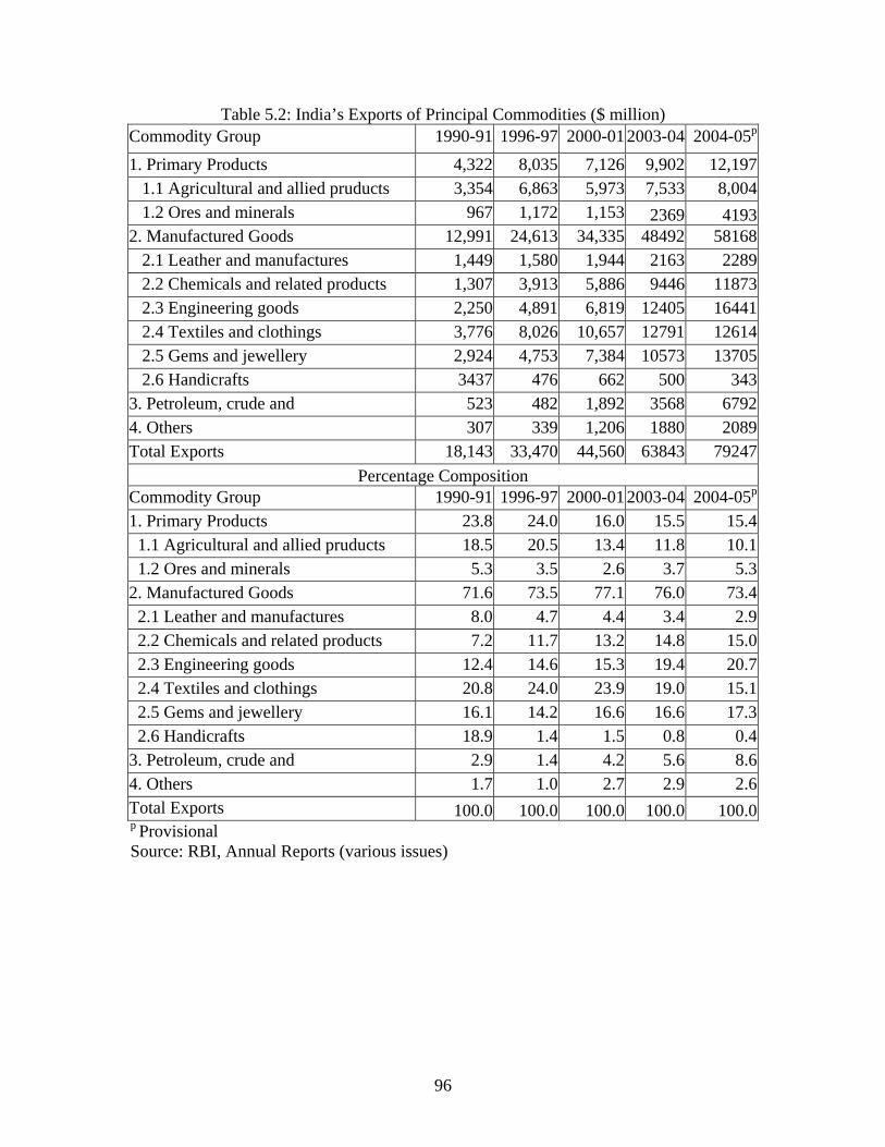
96

Table 5.2: India’s Exports of Principal Commodities ($ million) Commodity Group 1990-91 1996-97 2000-01 2003-04 2004-05p

1. Primary Products 4,322 8,035 7,126 9,902 12,197 1.1 Agricultural and allied pruducts 3,354 6,863 5,973 7,533 8,004 1.2 Ores and minerals 967 1,172 1,153 2369 41932. Manufactured Goods 12,991 24,613 34,335 48492 58168 2.1 Leather and manufactures 1,449 1,580 1,944 2163 2289 2.2 Chemicals and related products 1,307 3,913 5,886 9446 11873 2.3 Engineering goods 2,250 4,891 6,819 12405 16441 2.4 Textiles and clothings 3,776 8,026 10,657 12791 12614 2.5 Gems and jewellery 2,924 4,753 7,384 10573 13705 2.6 Handicrafts 3437 476 662 500 3433. Petroleum, crude and 523 482 1,892 3568 67924. Others 307 339 1,206 1880 2089Total Exports 18,143 33,470 44,560 63843 79247

Percentage Composition Commodity Group 1990-91 1996-97 2000-01 2003-04 2004-05p

1. Primary Products 23.8 24.0 16.0 15.5 15.4 1.1 Agricultural and allied pruducts 18.5 20.5 13.4 11.8 10.1 1.2 Ores and minerals 5.3 3.5 2.6 3.7 5.32. Manufactured Goods 71.6 73.5 77.1 76.0 73.4 2.1 Leather and manufactures 8.0 4.7 4.4 3.4 2.9 2.2 Chemicals and related products 7.2 11.7 13.2 14.8 15.0 2.3 Engineering goods 12.4 14.6 15.3 19.4 20.7 2.4 Textiles and clothings 20.8 24.0 23.9 19.0 15.1 2.5 Gems and jewellery 16.1 14.2 16.6 16.6 17.3 2.6 Handicrafts 18.9 1.4 1.5 0.8 0.43. Petroleum, crude and 2.9 1.4 4.2 5.6 8.64. Others 1.7 1.0 2.7 2.9 2.6Total Exports 100.0 100.0 100.0 100.0 100.0p Provisional Source: RBI, Annual Reports (various issues)

97

Table 5.3: India’s Imports of Principal Commodities ($ million) Commodity Group 1990-91 1996-97 2000-01 2003-04 2004-05P

Bulk Imports 10,971 16,365 20,816 29461 41880A. Petroleum, Petroleum Products and Related Material 6,028 10,036 15,650 20569 29844B. Bulk Consumption Goods 557 1,214 1,443 3073 3014C. Other Bulk Items 4,386 5,115 3,722 5819 9022NonBulk Imports 13,102 22,767 29,721 48688 65186A. Capital Goods 5,836 9,922 8,941 18279 22567B. Mainly Export Related Items 3,680 6,138 8,059 12717 16649C. Others 3,586 6,707 12,721 17692 25970Total Imports 27,073 39,132 50,536 78149 107066

Percentage Composition Bulk Imports 45.6 41.8 41.2 37.7 39.1A. Petroleum, Petroleum Products and Related Material 25.0 25.6 31.0 26.3 27.9B. Bulk Consumption Goods 2.3 3.1 2.9 3.9 2.8C. Other Bulk Items 18.2 13.1 7.4 7.4 8.4Non Bulk Imports 54.4 58.2 58.8 62.3 60.9A. Capital Goods 24.2 25.4 17.7 23.4 21.1B. Mainly Export Related Items 15.3 15.7 15.9 16.3 15.6C. Others 14.9 17.1 25.2 22.6 24.3Total Imports 100.0 100.0 100.0 100.0 100.0

p Provisional Source: RBI, Annual Reports (various issues)

The outward orientation of the economy since 1991 is best reflected in the share of

exports and imports in GDP. Merchandise exports as a proportion of GDP have doubled

from 5.8% in 1990-91 to 11.7% in 2004-05 (Table 5.1). Merchandise imports, too, have

exhibited similar upward movements from 8.8% to 17.2% of GDP in 2004-05 during the

same period. The Indian economy is increasingly becoming more integrated with the

global economy with foreign trade (exports and imports together) accounting for 29 per

cent of GDP in 2004-05. Correspondingly, merchandise exports from India have grown

from about US$18 billion in 1990-91 to US$79 billion in 2004-05 implying an

impressive trend growth rate of 11% per annum after the reforms. Imports rose by about

the same rate from US$23 billion to US$107 billion during the same period.

98

Among the major exports items, agriculture accounted for 10 per cent of total export

earnings, textiles and products 15 per cent, gems and jewellery 17 per cent and chemicals

and related products 15 per cent in 2004-05 (Table 5.2). The major groups on the imports

side are petroleum and petroleum products, capital goods and export related items (e.g.

pearls, precious stones, chemicals, textile yarns) respectively accounting for 28, 21 and

16 per cent of total import bill (Table 5.3)

India’s share in world exports has increased from 0.5% in 1991 to 0.8% by 2002. The

current account balance turned surplus during 2001-02 to 2003-043 after about three

decades and thus enabling current external receipts to pay for current external liabilities.

This was achieved primarily due to large expansion in invisible earnings on account of

remittances from abroad and software service exports together amounting to about 6 per

cent of GDP. In absolute terms, net inflows on account of transfers from abroad were of

the order of about US$21 billion and software service exports were close to US$17

billion in 2004-05.

Foreign direct investment (FDI) and portfolio investment in India has, however, been

modest at about US$ 4-5 billion in recent years. FDI flows have been less than 1 per cent

of GDP in India, while they account for 3-5 per cent of GDP in the East Asian

economies. While a larger quantum of FDI would enhance quantity as well as quality of

investment in India, its growth might remain modest in the near future. FDI has the

potential to play a critical role in manufacturing exports promotions through emerging

international value chain, technology transfer and productivity increase. India needs to

exploit this opportunity with an efficient strategy.

Continued overall surge in capital inflows has helped to build up foreign exchange

reserves that stand at US$130 billion by mid-2005, good enough to finance 14 months’

imports. A Committee set up by the RBI on Capital Account Convertibility (Tarapore

Committee) had suggested broadening the conventional criteria of judging adequacy of

3 Large rise in imports payments arising from oil price rise and domestic investment demand turned current account balance negative again in 2004-05.

99

foreign exchange reserves. Apart from import cover reserve adequacy ratio, it had

suggested consideration of other parameters like external debt servicing, and size,

composition and risk profile of capital flows. Given that the current level of foreign

exchange reserves are more than adequate to meet normal risks from volatility in

international flows, there is a need to examine continuation of the policy of accumulation

of the reserves. Reserve built up beyond an optimal level could be costly for the

economy.4

5.2 Foreign Exchange Rate An integral component of trade liberalisation in India was the move to a market

determined foreign exchange rate. This move again was carried out in a phased manner to

permit industry and trade to adjust and allow policy makers to monitor the system. The

system in operation at present might be described as ‘managed float’ that permits a

market determined competitive exchange rate while containing day-to-day market

volatility. The RBI manages the float by direct intervention in the exchange market as

well as by selective monetary and credit policy. The real effective exchange rate in recent

years has been nearly stable, though nominal effective rate has changed considerably

(Table 5.4). The range of variation in real effective exchange rate has been within 8% on

an annual average basis since early1990s.

4 See Lal et. al (2003), Sen (2004) and Singh and Srinivasan (2004) for a debate on this issue.

100

Table 5.4: Trends in Nominal and Real Effective Exchange Rate (Base 2000=100)

Nominal Effective

Exchange Rate (NEER) Real Effective Exchange

Rate (REER)

5-country

Index 10-country

Index 5-country

Index 10-country

Index 1991-92 180.4 170.1 103.72 100.441992-93 148.29 139.61 95.58 98.911993-94 136.74 131.57 92.11 90.641994-95 132.59 127.02 95.78 94.061995-96 121.25 115.4 95.17 92.441996-97 118.43 112.37 97.6 94.41997-98 118.49 114.54 102.26 100.411998-99 104.87 101.43 98.25 96.341999-00 100.99 99.05 96.94 96.252000-01 99.54 99.68 96.17 97.162001-02 98.47 98.54 99.36 99.82002-03 93.13 91.76 96.89 95.532003-04 92.07 88.7 101.21 97.33

Source: Economic Survey 2004-05 5.3 Growth and Poverty Effects Many countries have adopted trade reforms in recent decades in some form or the other.

Yet, there is very little unambiguous and general result in theory or empirics on the net

effect of trade liberalisation on poverty at the international level5. Trade liberalisation

does not automatically reduce poverty. But it could make an impact on poverty through

sustained economic growth. The international evidence on effect of trade liberalisation on

growth is mixed except for the general acceptance that closed regime has not helped a

country to maintain high growth on a sustained basis for several decades. Growth and

poverty impact of opening up of an economy has been very much circumstance specific.

Moreover, even when beneficial effect of trade liberalisation is seen at the aggregate level

due to more efficient allocation of resources, this by no means implies that all sections of

the society derive the benefit. Some economic agents gain in the process while others

5 See, for example, Dollar and Kraay (2002), Sachs and Warner (1995), Rodriguez and Rodrik (2001) and the review article by Winters et. al (2004).

101

lose6. If the losers happen to be poor, there might be need for a complementary

compensation mechanism to protect their welfare.

Did trade liberalisation process initiated in 1991 help poverty reduction in India? Our

detailed discussion earlier indicated that incidence of poverty deteriorated during the

early years of post-liberalization phase, but evidence of a fall in poverty was visible by

1999, though the extent of fall has been a matter of debate. The observed effects are

obviously the net result of a combination of several reforms and other developments.

Several authors have attempted to disentangle these effects by simulating the behaviour

of the economy with the help of different types of computable general equilibrium (CGE)

models. These economy wide models consider optimal behavior of economic agents like

consumers and producers and their interactions with autonomous agents like government

and are built around the database in a Social Accounting Matrix that takes into account

inter-sectoral flows. A flow diagram given in Figure 5.1 describes the effect of

international trade liberalisation on poverty. Trade liberalisation directly changes imports

and exports prices of tradable goods and in turn affects domestic prices. Prices in the

protected sectors are higher than world market prices before trade liberalization and such

prices fall when tariff or non-tariff barrier is reduced. Consumers benefit and producers

would lose in the process in the home country. On the other hand, if some sectors were

disprotected due to government export restrictions and their prices were lower than world

prices, consumers would lose and producers would gain because of higher prices in a post-

liberalised scenario. Trade liberalisation leads to reallocation of resources across sectors in

response to changes in domestic and external demand and supply conditions. Employment,

wages and profit levels corresponding to new equilibrium lead to changes in national

income and its distribution across income groups. Finally, both growth and distribution

factors determine poverty.

Exchange rate distortions could have major effects on the poor when their income

originates from tradable sectors. An overvalued currency would mean that producers

supplying their produce to the exports market do not receive competitive prices in

domestic currency which in turn depresses domestic prices too since domestic price

6 See, Winters (2004) who note Lloyd (2000) result that trade shock could benefit at least one household and hurt at least another household.

102

would be linked to world price for tradable. Imports on the other hand would be cheaper

across the board which disproportionately benefits producers with high import intensity.

Indeed, one reason for high import tariff prior to reforms was overvaluation of the rupee.

The effects of the depreciation of the exchange rate on imports prices in early 1990s were

offset, partly or fully, by simultaneous reduction of tariffs on many goods.

Figure 5.1: Flow Diagram Indicating Effects of Trade Liberalization on Poverty

Trade Liberalisation

Import and Export Price

Relative Prices of Domestic Products

Domestic Demand, Supply and Equilibrium Output

Economi c Growth

Imports and Exports Volume

Change in Real Exchange Rate

Wage and Profit Rate

Allocation of Labour and Capital

Income Distribution

Poverty Incidence

103

One CGE model by Panda and Quizon (2001) uses the Armington assumption that

domestic output and import (or export) in a sector are close, but not perfect, substitutes. A

distinctive feature of this model lies in its consideration of distribution of income by rural

and urban quartile groups, which helps in direct examination of changes in income of the

poor and the rich. Their simulation results over a base run that reproduces a social

accounting matrix for 1990-91 (the year just preceding initiation of liberalisation)

indicate that trade liberalization of the order observed during 1990s in manufacturing has

the following effects: (a) relative price of intermediate and capital goods become lower

by 7-9 per cent; (b) real exchange rate depreciates by about 8 per cent; (c) real investment

rises by 3.6 per cent primarily due to cheaper investment goods; (d) nonagricultural GDP

rises by about 0.3 per cent, while agricultural GDP rise is less than 0.1 per cent; (e) rural

households gain due to improvement in agricultural terms of trade and linkage with

nonagricultural sectors (rural areas receive about one third of nonagricultural income in

India); and (f) inequality in income distribution rises. Higher income groups gain more,

by 0.5 –1.1 per cent compared to 0.2-0.5 for lower income groups. Note that these results

are obtained from a stand-alone model for India and thus trade liberalisation impact

corresponds to that of a unilateral liberalisation process.

Their results show that effects of agricultural trade liberalization are dissimilar in some

respects to those of manufacturing in the Indian conditions. The effects arising from

removal of all trade barriers in agriculture are:

• Relative prices of foodgrains rise by 3-6 per cent. Terms of trade move in favour

of agriculture in case of either manufacturing or agriculture trade liberalization

due to the fact that manufacturing sector was typically protected and agriculture

was typically disprotected prior to the liberalization in India.

• Agricultural GDP expands by 0.8 per cent, but nonagriculture contracts

marginally by 0.1 per cent. The overall effect on real GDP is to raise it to about

0.3 per cent.

104

• The rural rich benefit the most by more than 2 per cent. Rural poor too gain,

though by less than 1 per cent. But the urban poor lose marginally due to rise in

foodgrain price and adverse manufacturing growth.

• A major factor that determines welfare effects of agricultural trade liberalisation

on the poor is whether the poor are net purchasers of cereals or not. Most of the

poor in rural India, being landless agricultural labourers or marginal farmers, are

net purchasers of cereals for whole or part of the year7. As such, a rise in price of

cereals hurts the poor8. Those poor farmers who are net sellers of cereals, on the

other hand, benefit from the price rise.

Parikh et. al (1997) use a sequential dynamic model for India to study impact of trade

liberalisation. Policy changes are introduced from 1993 and the impact examined over the

period 1993-2000. The authors find that real GDP rises by 4.5 per cent over the reference

run in the year 2000 implying an annual average GDP growth rate of 0.65 per cent per

annum during 1993-2000. An interesting result they report is that full agricultural trade

liberalisation leads to an immediate fall in agricultural output by about 1.7 per cent due to

short run disruption in agricultural production. Apart from allocative efficiency effect

under manufacturing trade liberalisation, they find that fall in relative price of investment

goods is a strong factor contributing to favorable GDP effect. As investment goods

become relatively cheaper, the same nominal investment rate can generate more real

investment. They report that consumer price index moves more favorably for the lower

income brackets leading to gain in their equivalent income9. Yet, calorie intake falls

marginally due to changes in consumption pattern. Another interesting argument made by

them is that India should be counted as a ‘large’ country in world rice market and

unrestricted rice exports could depress the world market price of rice leading to adverse

domestic welfare effects.

7 Some marginal and small farmers may also be ‘net purchasers’ of cereals because either they do not produce enough to meet their needs, or they are forced to sell cereals soon after harvesting to meet other expenditures and buy back cereals for own consumption during lean season. 8 This is in contrast to the experience in China where agricultural price rise benefited the poor (see, the China case study in this series, Bouche et. al, 2004). 9 Equivalent income refers to minimum income needed at base prices to achieve the same utility that a consumer enjoys currently.

105

Chadha et. al (2003) estimate the impact of Uruguay Round (UR) and Doha Round (DR)

agreement in a multilateral framework. They find India’s welfare gain measured by

equivalent variation is 0.68 per cent in UR scenarios involving phase-out of Multifibre

Agreement and manufacturing tariff reduction implied by UR. They obtain an additional

gain of 1.67 per cent due to DR scenarios developed as 33 per cent reduction in post-UR

tariff in agriculture, manufacturing and services. The output effect turns out to be 0.4-0.5

percent on an average. In the UR scenarios, the largest increase in employment takes

place in textiles, wearing apparel, trade and transport, mining, leather products and

footwear while employment loss occurs in all industrial sectors (led by machinery sector)

and in construction, private and public services. They also repeat their experiments

assuming unilateral liberalisation by India and find 1.4 per cent welfare gain.

So far as poverty effects of exchange rate movement are concerned, the structuralist CGE

models with cost based price equations capture the chain reaction arising from the cost

side10. Depreciation of domestic currency leads to price rise in tradable sectors affecting

exports and imports. If exports volumes are inelastic, domestic output might be adversely

affected due to depressed demand consequent upon inflation. On the other hand, if

exports and imports volumes were elastic, demand generation would expand domestic

output and contribute to growth. Poverty effects would operate mostly through the

growth effects.

In Parikh et. al (1997) real exchange rate (RER) is measured as the ratio of price of

tradables to that of nontradables. Agricultural trade liberalisation increases RER by 2 per

cent while trade liberalisation in all sectors increases it by 18 per cent. Resources would

naturally move in favour of tradables due to a rise in RER. But, they note that since some

tradable sectors were protected and some were disprotected prior to liberalisation, the

implication of an increase in RER is not straightforward on resource allocation. They find

long run price and resource reallocation effect is more in favour of agricultural sectors

that were disprotected earlier. Winters (2000) assumes that the non-traded sector is

‘informal intensive’ in India and suggests real exchange rate depreciation would expand

formal and shrink informal manufacturing employment.

10 See, for example, Sarkar and Panda (1991) for the Indian context.

106

Theory predicts that free trade would shift resource allocation towards those tradable

sectors which intensively use labour11, the relatively abundant factor in developing

countries. It is not clear, however, whether the theoretical prediction of substantial

resource reallocation towards labour intensive sectors has taken place in India. The

composition of export basket (Table 5.2) does not seem to support such prediction for

India. Composition of exports has moved away from labour intensive sectors like

agriculture, leather products, textiles and handicrafts.

Results from various CGE models indicate that trade liberalization could increase GDP

by 0.3-0.7 per cent with mostly favourable growth effects on poverty. These results are

produced by comparative static simulations and need to be interpreted carefully. While

these models are widely used12 and provide the links and causal mechanisms among

various variables very clearly, several critical parameters are not econometrically

estimated but obtained by calibration. The numerical simulation results thus represent

broad ex-ante predictions of effects of trade policy changes. The static efficiency gains

noted above are essentially due to relative price changes and movements from one point

on the production possibility frontier to another. The effects obviously depend on

magnitude of the shock or the extent of removal of trade barrier in the experiment. While

one might view them as a one-point gain, in practice the liberalisation process is carried

out in stages spread over several years and as such gains too might be spread thinly over

several years. Moreover, the experiments in stand alone country models often involve a

given international environment. One reason why the expected gains from agricultural

liberalisation have not been realized by India is that the experiments were carried out in a

situation where the world market prices of foodgrains were higher than the domestic

prices. The fall in world market prices of foodgrains subsequently reduced the level of

the distortion.

While the growth effects of trade liberalisation per se are relatively small one-time gains,

we should also take into account other related effects often accompanying trade

liberalisation like foreign investment flows and productivity increase. Foreign investment

11 This follows from the well-known Stolper-Samuelson theorem in a two-sector two-factor world with fixed factor supplies and flexible wages. 12 These are empirical counterparts of economy wide general equilibrium models in the Arrow-Debrue tradition and virtually the only tool for predicting impact of new policy regimes.

107

supplements domestically available savings to raise total investment in an economy, but

it might partly crowd out domestic investment particularly when it takes the mergers and

acquisitions route. Extent of crowding out is normally less for FDI than for other forms of

capital inflows (Brooks and Hill, 2004). The net effect of foreign investment flow is

likely to be investment and growth enhancing13. Overall net foreign investment flows in

India during the last decade have been only about one per cent of GDP, though it has

increased substantially during 2004 and 2005. Given the prevailing incremental capital

output ratio, the direct GDP effects would roughly be about a quarter percent of GDP.

Trade liberalisation and foreign investment inflows could be expected to lead to

productivity gains and bring in indirect benefit. Simulations carried out by Panda and

Quizon (2001) show that productivity gains of moderate order of 3 per cent per annum

could have considerable effect on growth by another half-a-percent. Productivity gains

could be realized from several sources: more competitive environment, access to

advanced technology from foreign collaboration, economies of scale due to expanded

market on external front. Again, CGE experiments carried out by Ganesh-Kumar et. al

(2005) indicate that comprehensive domestic reforms relating to investment are critical

for achieving higher growth.

Another related emerging issue in this context is trade facilitation, which refer to

expedition of the movement, release and clearance of goods including those in transit,

greater transparency and procedural uniformity of cross-border transportation of goods.14

Model experiments reported in Ronald-Holst et. al (2005) again indicate a growth effect

of about 10% for India over 20 years, e.g. less than 0.5% per annum.

Contribution of each of the several trade related components to growth is individually

small. But, taken together effects of trade and trade related policy package would not be

small and could push the growth rate of the economy by 1-2 percentage points. While the

effects of tariffs and quota reforms might have been mostly realised by now in India,

other effects are yet to be realised fully. These have the potential to place the Indian

economy on a growth path of 7-7.5 per cent per annum which is fairly good rate by

international comparison.

13 Using monthly data during December 1994 and March 1999, Das (2003) finds that actual flows of FDI have a positive effect on industrial production with a lag of 5 months. 14 See, Sengupta and Bhagabati (2005) for a discussion on this in the Indian context.

108

Will the poor gain from possible higher growth through this process? The answer would

largely depend on whether trade reforms contribute to an increase in inequality. The

evidence reviewed in chapter 2 point towards possibility of an adverse distributional

effect during the 1990s, though whether such a trend could be attributed to trade

liberalization is an open question. Some might argue that this could basically be

attributed to external sector policies and the move towards integration with the

globalization process. Adverse distribution effect might have partly neutralized the

potential gains from growth to the poor that could have accrued under invariant

distribution effect.

But, then both higher growth and higher inequality could be joint consequences of the

opening up policy. Pay packages in transnational companies are substantially higher than

those for comparable jobs in domestic companies leading to widening differential in

wage rates. The skill-biased technical progress of the 1990s in information and

communication sectors and consequent large demand for skilled and semi-skilled labour

has contributed to a rise in relative gap in wages between skilled and unskilled labour.

The recent growth of outsourcing has not led to large demand for labour that could be

classified as ‘unskilled’ by local standard. Thus, the most intensively used factor in these

newly emerged industries directly linked to world market is not likely to be the labour

that remains below the poverty line (official or $1 a day). The indirect benefits for

illiterate and poor labour class, of course, need not be insignificant as demand for

consumer goods by skilled labour expands through the multiplier process.

On the whole, however, if we consider elasticity of poverty with respect to per capita real

GDP, it has not changed after the reforms in both rural and urban areas15. In their review

of trade liberalization and poverty linkages, Winters et. al. (2004) conclude: “Despite the

methodological challenges to recent literature, there is no evidence to overturn the

traditional conclusion that growth, on an average, benefits the poor, nor to suggest that

growth generated by greater openness is any worse than other growth in this respect (and

15 Regression analysis of per capita real GDP on head count ratio in double log form with intercept and slope dummies for the post reform period does not indicate any significant change in the elasticity which remains round -1.0 for rural areas and -0.8 for urban areas. However, on a point-to-point basis, compared to 1983-87, the elasticity did fall considerably during the period 1987-1993 but recovered largely there after.

109

may even be better)” (P.81). If we consider the entire post-reform period, the Indian

experience seems to confirm this assertion.

Yet, the indication of a rise in inequality must attract policy attention to keep the possible

rise in inequality within moderate limits so that the adverse effect on poverty is not strong

enough to reduce the income elasticity of poverty and partly neutralize the positive

growth effect. Distributional conflict management has received more attention recently.

The National Employment Guarantee Act discussed earlier is a major move in this

respect16.

Another likely effect of opening up of an economy is an increase in volatility in prices. It

has been argued that India remained relatively insulated from the East Asian crisis

because of continued restrictions on its capital account convertibility. If world market

prices happen to be volatile as they do for several primary products, such volatility gets

transmitted to domestic market with all its consequences since domestic product market

prices for tradable goods are determined by world market prices. In the face of

agricultural subsidy regime maintained by developed countries, this could lead to serious

livelihood problem for poor farmers in India and other developing countries (see, Box

5.1). Monopoly purchase by a public agency might attempt to insulate farmers from

world price fluctuations, as was the case for cotton in India. While such a scheme

protects farmers from price volatility and provides stability, monopoly or monopsony

market structure might hinder integration with the world market and give rise to

monopsonistic profits.

The poor as such are less equipped to cope with adverse shocks than the non-poor. As

Box 5.1 shows trade liberalisation might aggravate it in the absence of complementary

domestic and international policies, which are important to enable the poor to benefit

fully from the new opportunities that opening up of the economy presents. There are

other types of complementary policies, particularly relevant for a large and diversified

country like India. We have noted the concentration of the poor in some parts country.

The low connectivity of these areas leads to high unit transaction costs and could turn an

otherwise tradable good to a virtually nontradable one. Government expenditure on 16 As Rodrik (1999) points out conflict management requires new and better institutions in developing countries.

110

physical and social infrastructure development then has a crucial role for integrating them

into mainstream of economic activities. India’s experience in this regard has been mixed.

There are areas where local market has been well connected with the world market

despite remoteness from a port, but there are vast areas in the countries which have as yet

remained isolated.

Box 5.1: World Price Volatility and Indian Cotton Growers In a liberalized trade regime, world market price volatility gets transmitted to

domestic market with all its consequences. Consider, for example, the case of cotton in the state of Maharashtra where the state government used to have a monopoly cotton procurement scheme (MCPS) that had a built in mechanism to pay cotton growers an assured price that was higher than the Minimum Support Price (MSP) of the central government taking into account higher costs conditions in the state and prevailing prices in the neighbouring states. Such a scheme provided insulation to farmers from world price volatility. The MCPS was abandoned in 2003 due to fiscal constraints by the state government. With trade liberalisation and privatisation of domestic trade, the cotton producers in India were seriously affected by world price fall in 2004. But, farmers in developed country were able to absorb the price shock due to the massive subsidy regime maintained in one form or another. The fall in cotton price and consequent erosion of profit was one of the factors that contributed to large number of farmers committing suicide in Maharshtra in an environment where cotton farmers are heavily indebted (Mishra, 2005). Cotton farmers do not have much option to shift to other crops in semi-arid Central India where poverty incidence continues to be high. Price volatility is a matter of life and death for such farmers.

Murphy, Lilliston and Lake (2005) note that cotton exports from US were sold

at an average price that was 47 per cent lower than the cost of production in 2003. The important policy questions to ponder about in this context are: Would world prices have been more stable had there been no large agricultural subsidy in the developed world? Should not India be justified to raise tariff on cotton so that its domestic price is nearer to the ‘free’ market price that would have prevailed in the absence of the subsidies?

111

5.4 Conclusion

To conclude, trade liberalisation in India has led to major changes in the macroeconomic

environment in India. The share of the tradable sectors in GDP has witnessed a large

increase and distortions in relative prices have been reduced sbstantially. Trade

liberalisation could affect poverty through both growth and distribution channels.

Observed incidence of poverty rose in India immediately after the beginning of the

reforms but fell subsequently. To what extent the observed happenings could be

attributed to trade liberalisation is a matter of debate. The rise in ex-post trend growth rate

by about 0.5 per cent per annum is similar in magnitude to the ex-ante model prediction

of trade liberalisation effects for India. The Indian evidence of the 1990s does not suggest

that the composition of the export basket has shifted considerably towards labour

intensive sectors. Part of the potential benefits of growth on poverty could have been

neutralized by the likely adverse effect of the opening up of the economy on wage

structure and income distribution. The recent growth of the outsourcing centres is not

likely to directly benefit the unskilled labour.

There is no firm evidence that the poor have benefited more from expansion of the

tradable sectors than the non-poor. The evidence discussed in earlier chapters suggest an

increase in urban-rural disparity in the post-liberalisation period, while inequality within

rural or urban areas might not have undergone any significant change. While the share of

the poor in national income might have remained the same or even fallen a bit since early

1990s, the poor have benefited largely from the volume effect. On the whole, Indian

evidence so far indicates that trade induced growth could benefit the poor nearly as much

as other forms of growth.

Trade liberalisation could lead to price and income volatility as it has happened for cotton

farmers in India. Also, tribal people who reside in remote parts of the country might not

be in a position to take advantage of the opportunities created by trade liberalisation.

Hence, one might reiterate the role of complementary policies for safety net and

infrastructure development.

112

113

Chapter 6 Monetary Policy and Financial Sector Liberalisation1

6.1 Evolution of Monetary Policy in India: Broad Phases The post-independence history of monetary and credit policy in India has

witnessed gradual transformation, keeping in pace with broader five-year plan and other

macro-economic goals and the tasks envisaged therein for the financial system. The most

dominant part of its role has been in building and nurturing institutions in the financial

system with a view to facilitating improvements in savings mobilisation and in

productive deployment of financial resources. The phases through which the conduct of

monetary policy has evolved, have coincided with the phases of institutional changes by

and large responding to the changing aspirations of the society. These phases could be

broadly classified into following periods:

A conventional phase in terms of monetary policy combined with a period of banking

consolidation and strengthening of banking regulations (1950-1967);

Credit initiatives, social control over banking and institutional build-up (1955-1967);

Bank nationalisation, vast branch expansion and significant structural changes in credit

distribution concurrently with an interventionist and structuralist stance of monetary and

credit policy (1969 to 1985);

A system of ‘monetary targeting with feedback’ achieved through the money-multiplier

process, with focus on the objective of price stability (1985-1991);

Formalisation of the transparent use of indirect instruments of monetary control

combined with financial sector liberalisation (1991-2002); and

The adoption of a ‘multiple indicators approach’ to monetary policy formulation (1998

onwards) followed by special emphasis on accelerating the flow of bank credit in favour

of agriculture, small and medium enterprises and micro-credit users (2002 onwards).

The interactions between instruments and outcomes are very complex. These complex

interactions assume pro-poor character essentially through sectoral credit strategies

(agriculture, rural areas and informal enterprises), but they are reinforced at the margin if

1 This chapter is an abridged version of the background paper written by S.L. Shetty.

114

supported by special credit schemes for the poor and targeted groups as well as institution

of micro-credit programmes.

6.2 Supply-leading approach to institutional credit structure Envisaging of such a complex sectoral credit strategy required a more wholesome

approach to institutional development in banking and finance area. The policy of bank

nationalisation and the associated public policies on banking and financial sector

development were predicated on the strong assumption of the need for promoting

financial intermediation by building institutions, expanding their geographical spread,

mobilising savings, and inducing better regional, sectoral and functional as well as small-

borrower reach of institutional credit in India. It was perceived that such a system of

supply-based and egalitarian institutional development could not be left to market forces

or to the initiative of private entrepreneurship. Also, the broad objectives embedded in

them, as set out above, were intertwined, for one could not be achieved without the other;

functional reach of credit, for instance, could not be attained without geographical spread

of banks as well as mobilisation of local savings.

A major aspect of banking development after the nationalisation of banks in July 1969

had been the rapid growth and territorial spread of branch network all over the country,

particularly in rural areas as well as in underdeveloped regions. The number of bank

branches increased from 1443 in December 1969 to 35,134 in March 1991 (Table 6.1).

What is more, the share of rural areas in the total number of bank branches improved

from 18 to 57 per cent during the same period. The shares of rural deposits and rural

credit in aggregate deposits and credit had also increased substantially. The Credit –

Deposit (C – D) ratio had increased significantly in rural and semi-urban areas (Tables

6.2 and 6.3). More significantly, the credit deposit ratio of rural branches exceeded the

prescribed target of 60 per cent by the mid-1980s.

The reform process of the 1990s has halted the process of institutional build-up

embedded in the supply-leading approach. Their branch expansion programme

monitored by the Reserve Bank of India (RBI) was disbanded, on March 31, 1995 and

the subject of bank expansion has been left to the commercial judgements of banks.

Consequently, the spread of branch network, particularly in rural and semi-urban areas as

115

well as in underdeveloped regions, has slowed down (Table 6.1). The credit deposit ratio

has declined in rural and semi-urban areas. However, due to new policy initiatives, the

situation has improved during 2000-2004 (Table 6.3).

The neglect of branch expansion after the 1990's has occurred on a distinct scale in big

size states of Bihar, Uttar Pradesh and Madhya Pradesh which account for half of the

poor (Table 6.4). These three states (including their satellite ones separated from them)

together accounted for 37.6 per cent of the country's total population in 2001, while the

share of these states in total bank branches was 29.0 per cent in March 1992 and 27.7 per

cent in March 2003. What is more, even though the proportion of bank deposits

mobilised in these states has not declined after the 1990s, the proportion of bank credit

obtained by these states has declined, and as a result, there has occurred a distinct decline

in their credit-deposit ratios.

Table 6.1: Spread of Bank Branch Network in India (Scheduled Commercial Banks including RRBs)

Rural Semi-Urban Total Period-end

Number of Bank Branches

Per cent to Total

Number of Bank Branches

Per cent to Total

Number of Bank Branches

Per cent to Total

December 1969 1,443 17.6 3,337 40.8 8,187 100.0

March 1991 35,134 56.9 11,566 18.7 61,724 100.0

March 1995 33,017 51.7 13,502 21.2 63,817 100.0

March 1996 32,981 51.2 13,731 21.3 64,456 100.0

March 2002 32,443 47.8 14,910 21.9 67,897 100.0

March 2003 32,283 47.4 15,042 22.1 68,078 100.0

March 2004 32,107 46.8 15,252 22.2 68,645 100.0

Notes: Decline in March 1996 is partly due to reclassification of centres based on the 1991 Census. Source: Reserve Bank of India: Basic Statistical Returns, various issues. (All tabulated data presented in

this chapter are from this source unless otherwise stated).

116

Table 6.2: Population Group-wise Credit-Deposit (C-D) ratio as per sanction and utilization

June 1980 March 1990 March 2000 March 2004 Year/

Population Group Sanction Sanction Utilisation Sanction Utilisation Sanction Utilisation

Rural 54.5 61.2 97.1 40.4 49.3 43.6 56.3

Semi-Urban 47.2 49.1 48.5 34.7 40.0 37.3 42.8

Urban 60.0 55.6 52.9 41.9 42.1 45.5 51.5

Metropolitan 87.0 69.9 58.0 78.9 73.2 75.9 67.7

All-India 67.2 60.7 60.7 56.0 56.0 58.2 58.2

Note: The phenomenon of migration of credit from the place of sanction to utilization elsewhere is responsible for the differences in C-D ratios as between sanction and utilization.

Table 6.3: Incremental Credit-Deposit Ratios By Population Groups: Credit Data Based on Utilization

(Amount in rupees, crore) [C-D ratios are in percentages] A. C-D Ratios as per outstandings of credit and deposit

March 2003 March 2000 March 1990 December 1980 Year/ Population

Group Credit

Outstanding C-D Ratio

Credit Outstanding

C-D Ratio

Credit Outstanding

C-D Ratio

Credit Outstanding

C-D Ratio

Rural 106,479 60.3 59,426 49.3 25,468 97.1 2,557 55.1 Semi-urban 104,149 43.1 64,790 40.0 17,597 48.3 4,090 47.9 Urban 142,874 49.2 79,590 42.1 22,428 52.9 5,242 56.5 Metro 402,465 70.9 256,274 73.2 38,820 58.0 11,785 81.1 All-India 755,969 59.2 460,081 56.0 104,313 60.7 23,674 64.0

B. C-D Ratios as per incremental credit and deposits March 2000 to March 2003 March 1990 to March 2000 Dec. 1980 to March 1990 Years/

Population Group

Increase in Credit

C-D Ratio Increase in Credit

C-D Ratio Increase in Credit

C-D Ratio

Rural 47,053 84.1 33,958 36.0 22,911 106.1 Semi-urban 39,359 49.3 47,193 37.6 13,507 48.5 Urban 63,284 62.3 57,162 39.0 17,186 51.9 Metro 146,191 67.2 217,454 76.8 27,035 51.6 All-India 295,888 65.1 355,768 54.8 80,639 59.8

117

Table 6.4: Proportions of Bank Deposits, Credit and

Credit-Deposit Ratios - Selected States March 2004 March 2002 March 1996 March 1992 December 1982 December 1972 Region

San- Ction

Utili- Sation

San- Ction

Utili- Sation

San-ction

Utili- Sation

San- ction

Utili- sation

San- ction

Utili- sation

San-ction

Utili-sation

Rajas than 55.7 62.8 48.4 55.4 45.4 45.3 55.6 59.3 70.1 74.1 48.6 54.5 Bihar 24.9 26.9 21.3 21.9 30.1 31.1 36.9 38.5 42.8 50.7 28.1 53.0 West-Bengal 49.5 53.8 45.8 49.2 55.2 53.3 52.8 51.0 59.3 54.1 76.0 65.5 Madhya Pradesh 46.9 50.1 46.6 50.3 56.2 60.6 61.0 63.2 58.2 61.2 46.6 51.8 Uttar Pradesh 33.1 38.0 29.9 34.3 33.8 35.0 42.5 45.3 44.7 47.3 36.9 42.2 Gujarat 42.2 54.8 44.1 54.7 52.9 56.9 52.4 57.3 52.0 53.9 56.4 64.6 Maharashtra 81.8 66.5 92.3 77.5 79.6 77.3 60.7 57.1 83.7 81.7 83.8 74.8 Tamil Nadu 93.1 96.1 85.4 88.5 94.9 94.4 89.0 89.1 94.6 94.5 109.5 110.0 All-India 58.2 58.2 58.4 58.4 59.8 59.8 57.7 57.7 67.1 67.1 66.4 66.4

A large number of districts particularly in the backward states began to experience in the

1990s reductions in credit delivery in relation to deposits that they generated. The number

of districts which had C-D ratios of less than 20 per cent about 20-28 districts (out of

401-478) was in March 1990, has increased to 105 districts (out of 565) in March 2000.

It may be argued that credit absorptive capacities of backward states and regions may

have eroded during the decade of the 1990s, but as is shown in a subsequent section, this

is only partially true; the supply of credit has been found to have fallen behind the

demand for it. And the resurgence of demand for correcting growing regional imbalances

has been responded to by the authorities in recent years by again pursuing an

interventionist credit delivery policy, particularly for agriculture, small and medium

enterprises and micro-credit users.

6.3. Special policy initiatives to promote larger credit absorption in backward

states/regions To mitigate the deteriorating credit deposit ratio in backward regions, special policy

initiatives were considered and put in place. Two special policy initiatives set out to show

larger credit absorption in backward regions have been: (i) bank investments in securities

and bonds of state governments and state-associated bodies; and (ii) resources placed by

banks with (NABARD) in rural infrastructure development fund (RIDF) which are

utilized for funding National Bank for Agriculture and Rural Development state

governments for rural infrastructure projects including irrigation projects; 2,16,099

118

projects for Rs 42,948.51 crore have been sanctioned under the RIDF up to the end of

March 2005.

Though inter-regional disparity remains, the north-eastern, eastern and central regions

show significant improvements in (credit utilization + investments + RIDF) to deposit

ratios. As shown in Table 6.5, with appropriate definitions, the number of states with C-D

ratios of 50 per cent and above have steadily increased, from 7 under CS-D ratio to 15

under CU-D ratio, to 21 under (CU+I) to D ratio and to 24 under (CU+I+RIDF) to D ratio,

as of March 2003. But, to add a caveat, C-D ratio based on utilisation plus investment

improves the position of underdeveloped regions, but it does so even for the advanced

southern region (Table 6.6). Further inclusion of RIDF benefits improves the C-D ratios

across all regions – developed as well as underdeveloped (Table 6.7).

Table 6.5: Number of States and UTs in Different

Ranges of C-D Ratio – March 2003 Range of CDR CS DR CU DR CU+I/D Ratio CU+I+RIDF/D<30 17 8 2 230-50 11 12 14 950-60 1 7 4 8>60 6 8 15 16Total

35 35 35 35

Note: CS/D: Credit as per Sanction to Deposit Ratio; CU/D Ratio: Credit as per Utilisation to Deposit Ratio; CU+I/D: Credit as per Utilization plus Investment to Deposit Ratio CU+I+RIDF/D: Credit as per Utilization plus Investment plus RIDF to Deposit Ratio

119

Table 6.6: Region-wise CDR (as per sanction) and C+I/D ratio (as per credit utilization) of scheduled commercial banks

March 1995 March 2000 March 2003 Region/ Year

CS/D CU+I/D CS/D CU+I/D CS/D CU+I/D

Northern 48.6 53.4 51.1 54.8 56.0 60.5

North-Eastern 35.6 68.8 28.1 48.9 27.4 67.0

Eastern 47.1 62.7 37.0 48.3 39.6 54.3

Central 39.0 57.3 33.9 48.5 33.3 49.9

Western 63.2 67.2 75.4 78.6 81.0 74.9

Southern 69.4 80.9 66.2 75.5 66.3 79.2

All-India 55.6 65.3 56.0 63.6 59.2 66.4

CS/D : Credit (as per sanction) + Investment to Deposit ratio CU+I/D: Credit (as per utilisation) + Investment to Deposit ratio

Table 6.7: Region-wise Credit plus Investment plus RIDF to Deposit Ratio March 2000 March 2003 Region/Year

CS/DR CU+I+RIDF/D CS/DR CU+I+RIDF/D

Northern 51.1 55.2 56.0 61.4

North-Eastern 28.1 50.2 27.4 69.4

Eastern 37.0 48.9 39.6 55.2

Central 33.9 49.6 33.3 51.3

Western 75.4 79.1 81.0 75.5

Southern 66.2 76.3 66.3 80.5

All-India 56.0 64.3 59.2 67.4

CS/D : Credit (as per sanction) + Investment to Deposit ratio CU+I+RIDF/D: Credit (as per utilisation) + Investment + Rural Infrastructure Development Fund (RIDF)

to Deposit ratio

120

6.4 Flow of Credit to agriculture and small-scale industries Since agricultural growth and decentralized industrialization have a crucial role to play in

the process of poverty reduction, special efforts were made to facilitate credit flow to

these sectors. Credit targets were combined with a series of other measures such as the

intensification of branch banking, the setting up of Regional Rural Banks (RRBs), and

the promotion of rapid expansion of bank credit for agriculture, small-scale industries and

other small and informal sectors based on the operation of ‘priority sector’ and other

sectoral targets. These measures yielded positive results in the pre-reform period. C-D

ratios of rural branches had improved and so also sectoral distribution of credit.

Agriculture A major achievement of the banking industry in the 1970s and 1980s was thus a decisive

shift in credit deployment in favour of the agricultural sector in particular. From a puny

level at the time of bank nationalisation, the credit share of the sector had moved to near

11 per cent in the mid-1970s and to a peak of about 18 per cent (the official target2) at the

end of the 1980s. But, thereafter its share of agriculture in total bank credit (both direct

and indirect) has declined to a low 10.9 per cent by March 2004 (Table 6.8). The number

of agricultural loan accounts which had reached a peak of 27.74 million in March 1992,

persistently declined thereafter and touched 20.35 million by March 2002 there has

occurred a fractional increase thereafter to 21.30 million by March 2004 (Table 6.8)

2 Earlier, there was a target of 18 per cent of net bank credit to agriculture in the form of direct advance, but subsequently, such target was allowed to be achieved by including not more than 25 per cent also in the form of indirect credit. Besides, a number of other provisions like the contribution permitted for the NABARD’s rural infrastructure development fund (RIDF) to the extent of 1.5 per cent of net bank credit, have contributed to the reduction in the effective share of agricultural credit. In 1993, the RBI had asked the banks to prepare special agricultural credit plans and increase their credit disbursals to agriculture by 20 per cent annually so that the effective target of 18 per cent of net bank credit could be met.

121

Table 6.8: Outstanding Credit of Scheduled Commercial Banks against Agriculture and Small-scale Industries

Agriculture

Other Small Scale Industries

No. of Per cent Per cent No. of Per cent Per cent Year Accounts to All India Amount to All India Accounts to All India Amount to All India

Dec-72 1371975 31.6 50091 9.0 172685 4.0 65926 11.9Dec-75 3042170 41.3 107058 10.7 262301 3.6 117796 11.8Dec-78 7059556 47.2 234233 13.2 498914 3.3 207973 11.7Dec-81 11231727 50.5 486330 17.1 765431 3.4 353315 12.4Dec-84 15844321 50.2 807286 17.5 1714985 5.4 622602 13.5Dec-87 21907916 47.4 1211236 17.7 2868501 6.2 880023 12.9

June -89 23571891 45.2 1526580 17.3 3364221 6.5 1182063 13.4Mar-90 24520595 45.5 1662607 15.9 1606146 3.0 1198563 11.5Mar-93 26216787 42.2 2206022 13.6 2070868 3.3 1826393 11.2Mar-96 24188573 42.7 2880896 11.3 1752054 3.1 2582270 10.1Mar-99 19788385 37.8 4088926 10.7 2029920 3.9 3142843 8.2Mar-00 20532891 37.8 4563827 9.9 2126150 3.9 3506987 7.6Mar-01 19843289 37.9 5173035 9.6 1742544 3.3 3690487 6.9Mar-02 20351184 36.1 6400855 9.8 1572798 2.8 3197030 4.9Mar-03 20840434 35.0 7593522 10.0 1431421 2.4 3794034 5.0Mar-04 21304168 32.1 9624504 10.9 718056* 1.1 3843255 4.4

Source: RBI’s Basic Statistical Returns, various issues. * This does not appear to be correct; the error is in the source.

The commercial banks have a relatively low credit to GDP ratio3 for agriculture as

compared with other sectors (Table 6.9). Though the other sectors have been traditionally

absorbing larger credit per output, there are a few important considerations which call for

an expanded credit base for agriculture in the current phase. First, the proportions of paid-

out costs in terms of modern inputs have considerably increased in agriculture over the

years. Second, vast diversifications are taking place in agriculture away from crop

husbandry and in favour of horticultural and livestock products, which require higher

amounts of short-term and investment credit from the institutional sector. Finally, the

proportion of work force dependent on agriculture remains at near 60 per cent. Likewise

a supply-leading role for the financial system also envisages the seeking of potential

bankable schemes in relatively poorer regions. Interestingly, it is found that

3 Though credit outstanding is a stock concept and GDP a flow concept, the trends in the credit to GDP

ratio are still valid because the bank credit use is of a revolving type and the whole of it goes to support the production process of a given period. The same should be true of credit to SDP ratios.

122

underdeveloped regions have hardly lagged behind the advanced regions in generating

bank deposit growth. On the other hand, bank credit to SDP ratios have remained unduly

low in respect of underdeveloped regions and states as compared with those in the

advanced regions. It must be again mentioned in parenthesis that in regard to both

agriculture and underdeveloped regions, there have been improvements in the recent

period in the application of commercial bank credit per unit of output.

Table 6.9: Trends in Bank Credit to GDP Ratios: By Sectors

Sectoral Groups

Credit to

GDP Ratio (Per Cent)

Credit to

GDP Ratio (Per Cent)

Credit to

GDP Ratio (Per Cent)

2003-04 2000-01 1995-96 Agriculture and Allied Activities 15.0 10.4 8.9

Industry 48.4 44.5 36.2 Others 32.1 24.3 20.6 Total GDP 32.5 26.2 21.7 1990-91 1985-86 1980-81 Agriculture and Allied Activities 11.0 12.8 15.2

Industry 38.9 45.3 62.3 Others 19.9 24.7 41.3 Total GDP 22.4 26.4 36.9

Government has been intervening in the recent years and putting pressure on banks to

expand farm credit. This has yielded desirable results. According to recent NABARD

data on total credit flow for agriculture including that from cooperatives, during the five-

year period 1999-2000 to 2003-04, crop loans4 (production credit) have expanded at the

rate of 17.3 per cent per annum, while term loans have grown at the rate of 15.4 per cent

per annum (Table 6.10). With the introduction of special agricultural credit plans, the

4 Crop loans have generally constituted 66 per cent of the total farm credit. While

cooperatives give just about 20 per cent of total term credit, commercial banks and RRBs

provide over 80 per cent.

123

share of commercial banks and RRBs in total agricultural credit has increased from 60

per cent in 1999-2000 to 69 per cent in 2003-04, while that of cooperatives has slipped

from 40 per cent to 31 per cent (Table 6.12). Doubling of agricultural credit in three

years, 2004-05 to 2006-07, has been a major step envisaged by the government.

NABARD has already reported a 40 per cent increase in farm credit during 2004-05,

bringing 7.9 million new farmers under the institutional fold.

Table 6.10: Flow of Total Agricultural Credit from All Institutional Agencies

(Rs. Crore) Year

Short term

Growth rate (%)

Term credit

Growth rate (%)

Total

Growth rate (%)

1995-96

14525 (65.9)

-

7507 (34.1)

- 22032 (100)

-

1996-97

16998 (64.4)

17.0

9413 (35.6)

25.4

26411 (100)

19.9

1997-98

20640 (64.6)

21.4

11316 (35.4)

20.4

31956 (100)

21.0

1998-99

23903 (63.9)

15.8

12957 (36.1)

14.5

35860 (100)

12.2

1999-00

28965 (65.3)

21.1

17303 (37.4)

33.5

46238 (100)

28.9

2000-01

33314 (63.9)

15.0

19513 (36.1)

12.8

52827 (100)

14.3

2001-02

40509 (65.3)

21.6

21536 (34.7)

10.4

62045 (100)

17.4

2002-03

45586 (65.5)

19.1

23974 (34.5)

11.3

69560 (100)

12.1

2003-04 54977 (63.2)

20.6 32004 (36.8)

33.5

86981 (100)

25.0

CAGR 1995-96

to 2003-04

18.1

18.7 18.4

Issuance of Kisan Credit Cards (KCCs) has been yet another step in the direction of

expanding farm credit. An average of about 90 lakh KCCs have been issued during the

past five years 2000-01 to 2004-05, taking the aggregate to 511 lakh. Hitherto, KCCs

were only for crop loans but in 2004-05, their scope was expanded to cover term loans.

Hence, commercial banks have replaced cooperatives as the maximum issuers of KCCs.

124

125

Table 6.11: Agency-wise break-up of term credit for agriculture (Rs.Crore)

Year

Coops

Growth rate (%)

Comm. Banks

Growth Rate (%)

RRBs

Growth rate (%)

1995-96 2148 (29) 4827 (64) 532 (7) 1996-97 2616 (28) 21 6234 (66) 29 563 (6) 6 1997-98 3190 (28) 22 7482 (66) 20 644 (6) 14 1998-99 3386 (26) 6 8821 (68) 18 750 (6) 16 1999-00 3518 (20) 4 13036 (75) 48 749 (4) - 2000-01 4218 (22) 20 14321 (73) 9 974 (5) 30 2001-02 4776 (22) 13 15683 (73) 9 1077 (5) 11 2002-03 3956 (17) -17 18724 (78) 19 1294 (5) 20

CAGR 10.2 21.6 13.6 Small-Scale Industries Next to agriculture, the small-scale industrial (SSI) sector occupies a pivotal position in

terms of employment and output share in the economy. Apart from sectoral dispersal and

wider promotion of entrepreneurship, the small-scale industries have a regional

dimension in that the SSI units are scattered all over in the nooks and corners of the

country. Immediately after the introduction of social control and subsequent bank

nationalisation, banks found the small-scale industries as lucrative target for lending.

Hence, the share of SSI units in total bank credit shot up from 6.9 per cent in June 1968

to 12.0 per cent in June 1973. Thereafter, it was sustained in the range of 11 to 13.5 per

cent until the early 1990s. However, there has occurred a steady and drastic fall in the

share of bank credit in favour of small-scale industries from 13.4 per cent in March 1989

to as low as 5.0 per cent in March 2003 and that of artisans and village industries from

0.9 per cent to 0.7 per cent. The number of bank loan accounts in respect of the SSI

sector has dropped from a peak of 33.64 lakh in June 1989 to 14.31 lakh in March 2003 -

a loss of near 20 lakh.

Overall, the momentum of better credit delivery for agriculture and small-scale

industries, as also the underdeveloped states, noticed in the 1980s, has not been sustained

in the 1990s and thereafter. While a few other factors may have played a role in adversely

affecting the momentum of growth to agriculture and small scale industries and regions

126

since the beginning of the 1990s, the loss of momentum in the task of credit delivery for

them by scheduled commercial banks may appear to have had a part in it.

6.5. Flow of Credit to Small borrowers and other vulnerable groups Between December 1972 and June 1983, there were 21.2 million additional bank loan

accounts in the aggregate added and nursed by the scheduled commercial banks, of which

19.8 million (93.1 per cent) were accounts with Rs 10,000 or less of credit limits. This

trend continued for another decade up to March 1992 (despite the loan waiver scheme

effective March 15, 1990). But the momentum was lost in the 1990s. There has been an

absolute decline of about 13.5 million in the aggregate bank loan accounts between

March 1992 and March 2001 and a much larger decline of 25.3 million in the redefined

small borrowal accounts with credit limits of Rs 25,000 and less. On the other hand,

borrowal accounts with higher credit limits of above Rs 25,000 have shown an unusually

large increase of 11.8 million as compared with only 2.1 million increase in them during

the preceding decade (December 1983 to March 1992). Even in the recent period

between March 2001 and March 2004, while there has been an addition of 14.3 million in

total loan accounts, small borrowal accounts have experienced an absolute fall of 0.5

million (Table 6.12).

Table 6.12: Trends in the Number of Small Borrowal vis-à-vis other Bank Loan Accounts

Total Bank Borrowal Accounts (In Lakh)

Small Borrowal Accounts of Rs,25,000 or less

(In Lakh)

Other Bigger Accounts (In Lakh)

Period-End

Number Increase over the previous period

Number Increase over the previous

period

Number Increase over the previous

period

Dec-1983 277.48 - 265.21 - 12.27 - March 1992 658.61 381.12 625.48 360.27 33.12 20.85 March 2001 523.65 (-) 134.95 372.52 (-) 252.96 151.13 118.01 March 2004 663.90 140.25 367.66 (-) 4.86 296.24 145.11 6.6. Impact of credit contraction on poor households First, nearly 80 per cent of small borrowal accounts have been in rural and semi-urban

areas and hence their contraction is sure to hurt the borrowers in such areas. Second,

127

about 22 per cent of the number of small accounts and 18.1 per cent of the amount

outstanding of such accounts have been in respect of women borrowers; over the years

this proportion has edged up implying that women borrowers have increased their share

of bank borrowings. Such is not the case with the borrowers amongst scheduled castes

and scheduled tribes; their share has remained generally static between 1993 and 1997;

the shares of women in these groups are also broadly the same. Even within this small

borrower category, smaller loans up to Rs 7,500 had accounted for 80.5 per cent of the

number of accounts and 50 per cent of the loan amount outstanding in March 1993,

which slipped to 64 per cent and 32 per cent, respectively by March 1997. The bulk of

the small borrowal accounts have been for agricultural and allied activities. Finally, about

50 per cent of the small borrowal accounts have been granted under special asset-creating

employment programmes like the IRDP, SEEUY, SEPUP, DRI and others. Regional

rural banks (RRBs) stand out as the banks serving the small borrowal accounts; it is more

so in rural areas. Many of these phenomena are getting further reinforced in the more

recent period. Small borrowal accounts have about two-thirds of credit outstanding as

standard assets, which is somewhat lower than that for the public sector banking system

as a whole at 88 per cent (RBI 2001:59). Standard assets of small borrowal accounts have

risen with the size of loans but have been higher for agricultural activities than for

industry, trade and transport except for personal and professional loans; the latter

categories thus have weaker assets.

6.7 Micro Credit Movement in India The micro-credit system in India has by now received substantial official support. The

RBI has set up a special cell in order to liaise with NABARD and micro-credit

institutions for augmenting the flow of credit to this sector. Defining micro credit as

“provision of thrift, credit and other financial services and products of very small amount

to the poor in rural, semi-urban areas for enabling them to raise their income levels and

improve living standards”, the RBI has issued a number of guidelines to be observed by

banks in rendering microcredit assistance.

128

Progress made in the NABARD’s SHG-bank linkage programme Presenting the progress made in the SHG-bank linkage programme (NABARD 2005),

NABARD has stated that cumulatively, 16.18 lakh SHGs obtaining bank loans

aggregating Rs 6,898.46 crore with refinance support of Rs 3,086 crore (Table 6.13(A))

covered near 200 lakh poor households. These numbers are rapidly increasing now.

SHGs comprising only women members have constituted 90 per cent; with timely loan

repayment (95 per cent). There has been substantial regional concentration of SHGs, with

the southern states accounting for 67 per cent of the total SHGs credit linked and 81 per

cent of the total amount of bank loan disbursed. Andhra Pradesh has alone accounted for

36 per cent of the SHGs credit linked as at the end of March 2004. This situation is,

however, claimed to be undergoing a change as may be seen in the latest data provided

by NABARD. However, it is important to note that for the BIMARU states, the

proportion of SHGs in the all-India total has remained at about 15-17 per cent. (Table

6.13(B)).

Table 6.13(A): NABARD: Bank-SHG Credit Linkage Programme Cumulative Progress up to 2004-05

Year-End (April-March)

No. of SHGs linked SHGs Refinanced (Number)

Bank Loans (Rs. Crore)

Refinance by NABARD (Rs. Crore)

2000-01 263,825 213,213 480.87 400.74 2001-02 461,478 340,131 1026.34 796.47 2002-03 717,360 493,634 2048.67 1418.80 2003-04 1,079,091 611,043 3904.20 2124.24 2004-05 1,618,476 824,888 6898.46 3085.91

* In the 2000-01 report, SHGs are excluding those not covered under refinance Source: NABARD's Annual Report 2004-05 and Various Issues

129

Table 6.13(B): Cumulative Growth in SHG-Linkage in Priority Status

(Number of SHGs as on March 31st)State 2002 2003 2004 2005 Assam 1024 3477 10706 31234 Bihar 3957 8161 16246 28015 Chhattisgarh 3763 6763 9796 18569 Gujarat 9496 13875 15974 24712 Himachal Pradesh 5069 8875 13228 17798 Jharkhand 4198 7765 12647 21531 Maharashtra 19619 28065 38535 71146 Madhya Pradesh 7981 15271 27095 45105 Orissa 20553 42272 77588 123256 Rajasthan 12564 22742 33846 60006 Uttar Pradesh 33114 53696 79210 119648

Uttaranchal 3323 5853 10908 14043

West Bengal 17143 32647 51685 92698

Total for 13 states 141804 (30.7) 249462 (34.7) 397464 (36.8) 667761 (41.2)

BIMARU States 57616 (12.5) 99870 (13.9) 156397 (14.5) 252774 (15.6)

All-India Total 461,478 717,360 1079,091 1618,476 Note: Figures in brackets represent percentages to All-India totals Source: NABARD, Annual Report 2004-05. p.41

Table 6.14: Progress Under SIDBI Foundation for Micro Credit (SFMC) (Amount in Rs crore)

Year Amount Sanctioned

Amount Disbursed

Number of SHG’s Involved

Outstanding Loan Portfolio of SIDBI (Amount)

Cumulative sanctions of assistance (Amount)

Cumulative Total number of poor persons benefited (lakh)

1999-2000 21.90 14.03 - - 52.61 3.14 2000-01 28.28 19.45 20530 33.24 (1.50) 81.05 4.42 2001-02 41.70 21.79 28436 43.45 (1.51) 122.75 7.28 2002-03 38.51 31.04 - - 161.26 8.62 2003-04 70.84 66.31 - 91.21 232.08 10.41 2004-05 189.73 145.06 - 199.21 421.81 15.10

Figures in brackets represent NPAs of the total portfolio Source: SIDBI Annual Reports, various issues.

SIDBI Foundation for Micro Credit (SFMC), launched effective from January 1999, has

sanctioned financial assistance of Rs 189.73 crore during 2004-05 as compared with Rs

70.84 crore in 2003-04 (Table 6.14). The cumulative assistance since inception

aggregated Rs 421.81 crore extended through 209 MFIs said to be benefiting over 15.10

lakh poor people, mostly women.

130

The micro finance movement in India has shown significant potential, and with intensive

official support, the coverage has significantly expanded – which, as the institutional

visions portray, is likely to be further intensified. The RBI has also expanded the scope

by giving freedom to institutions to charge interest rates at their own discretion and more

importantly, to cover not only consumption and production loans but also credit needs of

housing and shelter improvements. Self-Help groups involve thrift as well as credit

arrangements. NABARD and SIDBI have provided for SHGs and SHG members scope

for capacity building through training and other inputs by NGOs. Peer monitoring helps

better credit recovery. Finally, the SHG movement so far has shown that the outcomes

have gone beyond thrift, credit and economic well-being; it has served as an instrument

of social change essentially out of the empowerment of women. Improvement in literary

levels and children’s education particularly in awareness of girls’ education, housing

facilities, abolition of child labour, decline in family violence, and banning of illicit

distilleries in the villages - have all been reported in different studies. Women have

acquired better communication skills and self-confidence; they have also acquired better

status within families.

6.8. Attempts at regaining the momentum of credit delivery for small and informal

sector borrowers

Apart from more intensified flow of bank credit for agriculture, small and medium

enterprises and micro-credit groups, a number of initiatives have been taken by the

authorities in the recent period to correct the loss of momentum suffered in the 1990s in

terms of halting the growth of branch network in rural areas and reduced flow of credit

for small and informal sector borrowers.

First, the system of agency banking has been proposed whereby two models, namely,

business facilitator model and business correspondent model, have been recommended to

the banking industry. Under the business facilitator model, it has been envisaged that

banks could use a wide array of civil society organizations (CSOs) and others for

supporting them by undertaking non-financial services. The facilitators that would

provide support services for effective delivery of financial services, are NGOs, farmers

clubs, rural multi-purpose kiosks/village knowledge centres, and many others. Likewise,

131

under the business correspondent model, institutional agents/other external entities may

support the banks for extending financial services. The business correspondents would

function as “pass through” agencies to provide credit-related services such as, disbursal

of small value credit, recovery of principal/collection of interest and sale of micro

insurance/mutual fund products/pension products (RBI 2005, p.19).

Second, with the widening of the scope of RRBs’ functioning, they have been permitted

to set up ATMs, issue debit/credit cards and also to handle pension/Government business

as sub-agents of banks authorised to conduct government business.

Third, the Reserve Bank has advised scheduled commercial banks and RRBs with the

support of detailed guidelines to introduce a general credit card (GCC) scheme for their

customers in rural and semi-urban areas. The GCC will operate like the kisan credit card

(KCC) but there will be no linkage to purpose or end-use of funds or security. The GCC

can also be used for withdrawing cash against the limit sanctioned. Women will be given

preferential treatment under the GCC Scheme. Banks have been asked to utilise the

services of local post offices, schools, primary health centres, local government

functionaries, farmers' associations/clubs, etc., for sourcing of borrowers for issuance of

GCC.

Finally, with a view to giving small borrowers an opportunity to settle their non-

performing accounts with banks and become eligible for fresh finance, all scheduled

commercial banks (including RRBs and Local Area Banks) have been advised to provide

a simple mechanism for one-time settlement (OTS) of loans for the principal amount up

to Rs. 25,000 which have become doubtful or loss assets as on September 30, 2005.

State-Level Bankers Committees have also been asked to evolve state-specific guidelines

for loans granted under Government- sponsored schemes. This scheme will not cover

cases of frauds and malfeasance.

132

Chapter 7 Inter State Contrasts in Poverty Reduction: A Synthesis of

Selected States5

7.1 Introduction

State level analysis can capture diverse experiences of the states in poverty reduction as

well as complement the macro analysis. Poverty at the state level is likely to be affected

by the macroeconomic policies as well as state specific policies. The state reports provide

comprehensive picture of four selected states: Bihar, Orissa, Rajasthan and Tamil Nadu.

These states have diverse characteristics with regard to structure of poverty, institutional

structure and the development process. This chapter focuses on the following questions:

what are the factors that explain the differences in poverty reduction between states?

How do the states differ in terms of their approach to poverty reduction and what factors

have contributed to varying performances? It draws on the findings of the four state-level

reports.

7.2 States’ Profiles

Bihar, the second most densely populated state in the country, is endowed with very rich

soil and irrigation to sustain agriculture. About 17% of the geographical area is covered

by forests; while 47% falls under agriculture. Nearly 50% of agricultural land is irrigated

of which 65% is commanded by wells ( Table 7.1) . Nearly 90% of the population is rural

based, that depends on agriculture for its livelihood. The recurrence of floods affects the

people living on agriculture and the poor, vulnerable to such shocks suffer the most.

Large incidence of landless labour and rigid agrarian structure hinder agricultural

growth. After the bifurcation of the state into Bihar and Jharkhand in 2000, Bihar has lost

its major mining and industrial areas to Jharkand6.

5 G. Mythili is the author of this Chapter. This chapter draws generously on respective state reports prepared by (a) Ashok Mathur and Alakh N. Sharma for Bihar (b) Kailas Sarap for Orissa (c) Vidya Sagar for Rajasthan and (d) K.V. Palanidurai for Tamil Nadu. 6 Data and discussion on Bihar included in this chapter pertain to undivided Bihar.

133

Orissa is characterized by the highest incidence of poverty, very low per capita income

and low agricultural productivity. Agriculture covers 39% of the geographical area, of

which irrigated area is only 35%. Canal irrigation is the predominant source of irrigation

accounting for 45% of the net irrigated area. The agricultural sector is characterized by

higher proportion of landless labour, declining land- man ratio and high incidence of

tenancy. State income is marked by high annual fluctuations owing to frequent

occurrence of drought in western regions and floods in coastal regions. 85% of the

population live in rural areas out of which about 41% are tribes. It has a forest cover of

36% of total area; tribal population depending on forest is very pronounced in this state.

Orissa also suffers from structural rigidities in the agrarian structure.

Rajasthan is known for its diversity in resources and activities. About 60% of its area is

desert with sparse population and 81% is arid or semi-arid that receives low rainfall.

Nearly 45% of the area falls under agriculture with an irrigation ratio of mere 33%. Its

irrigation resource is unevenly distributed across its regions.

(Table 7.2). About three-fourths of the population lives in rural areas. Tribal and SC

communities account for 30% of its population. The state has a rich historical and

cultural heritage and it attracts both national and international tourists. Both handicrafts

and tourism have huge employment potential. Development of rural non-farm sector

enables the poor to cushion shocks resulting from failure of crops.

Tamil Nadu being one of the fast growing states in the country is the second most

urbanized state as urban population accounts for 44% of total population. Sustained

growth, growing IT and manufacturing sectors characterize the economy. Tamil Nadu

has witnessed demographic transition in the last decade. High female literacy and women

empowerment are additional features. Agriculture covers 42% of the total geographical

area, of which irrigated area accounts for 53%. Surface water was fully tapped; and

groundwater to an extent of 60% was tapped. Water scarcity has emerged as a major

constraint on agricultural growth. The state also suffers from land degradation, viz. water

logging and saline affected area is significant, around 2.23% of geographical area.

134

Table 7.1 : Major Characteristics of the States – 1999-2000 States Populat

ion density- Person per sq.km

% of rural population

% of SC and ST population

% of area under forest

% of net sown area to total area

Cropping intensity

% of net irrigated area to net area sown

% of canal irrigated area

Bihar 880 90 17 17.0 42.9 1.35 50 28 Orissa 236 85 39 36.0 39.0 1.35 35 45 Rajasthan 165 77 30 7.6 45.3 1.21 33 27 Tamil Nadu

478 56 24 16.4 42.0 1.20 53 28

Source: Census Reports and CMIE, Agriculture Table 7.2: Region Specific Key Farm Statistics – by NSS regions- 1999-2000

States

Regions Irrigated Area %

Farm output per hectare

Farm Output per worker

Unit (at 90-93 prices)

‘000 Rs.

(at 90-93 prices)

’000 Rs. Southern Bihar

24 5.1 1.7

North Bihar 75 6.3 2.5

Bihar

Central 78 7.2 2.8 Coastal 26 4.7 2.5 Southern 6 4.4 1.6

Orissa

Northern 17 4.0 1.9 West 27 3.2 4.9 North East 61 5.6 5.9 Southern 47 4.5 2.4

Rajasthan

South Eastern

76

7.4 7.8

Coastal North

75

24.3 12.7

Coastal 77 14.4 8.4 Southern 70 16.4 6.9

Tamil Nadu

Inland 66 22.2 13.1 Source: Himanshu, 2005

135

7.3 Poverty Profile Poverty indicator, as measured by Head Count Ratio7, for the four selected states in early

1970s and 1999-2000 are given in Table 7.3. According to the Planning Commission

estimates in 1999-2000, poverty incidence was more than 40% in Bihar and Orissa as

against all-India figure of 26%. Rural Bihar alone accounts for 21% of the country’s rural

poor. Poverty incidence is the least in Rajasthan, 15% followed by Tamil Nadu, 21%.

Table 7.3: Poverty Index (Head Count Ratio) for Selected States

States

1973-74 1999-2000

% change per annum from 73-74 to 99-2000

Bihar 61.91 42.60 -1.20 Orissa 66.18 48.14 -1.05 Rajasthan 46.14 14.78 -2.61 Tamil Nadu 54.94 21.12 -2.37 All India 54.88 26.10 -2.02

Source: State Reports and National Human Development Report, 2001

In Rajasthan and Tamil Nadu poverty has declined by about 2.5% per annum between

1973-74 and 1999-2000. This reduction is faster than the all India figure of 2% per

annum. In Orissa and Bihar, the reduction is slower at 1% and 1.2% respectively. As per

official estimates, poverty almost remained stagnant in Orissa, between 1993-94 and

1999-2000, whereas Rajasthan and Tamil Nadu have registered a reduction of about 7%

per annum between 1993-94 and 1999-2000. In Tamil Nadu and Rajasthan the urban

poverty was higher than the rural poverty in the nineties8 (Chapter 2 , Table 2.4).

7 The poverty index based on poverty gap and squared poverty gap more or less depict the same trend as does head count ratio. 8 According to the available alternative estimates (Deaton and Dreze, 2002) , the rural poverty seems to be significantly underestimated in the official statistics. However it is to be mentioned that rural and urban poverty estimates are not exactly comparable as they are based on different poverty lines.

136

Figure 7.1 Percentage Change in Incidence of Poverty between 1973-74 and 1999-2000

-80-70-60-50-40-30-20-10

01

States

perc

enta

ge c

hang

e in

pov

erty

in

cide

nce

BiharOrissaRajasthanTamil Nadu

Inequality index A major factor that contributed to poverty decline in rural Rajasthan is redistribution, that

is reflected in the falling Gini inequality index of monthly per capita expenditure in rural

areas consistently from the early 80s till 2000 (Table 7.4). It registered a decline of 3.27

percent per annum between 1993-94 and 1999-2000 against a measly decline of less than

1% per annum in other states. This may be attributed to diversified nature of income

sources. It is worth mentioning that in rural Rajasthan, livestock as a source of income

protects the rural poor from fluctuations in crop income. It yields more stable income

than the crop sector. Further, distribution of livestock asset shows less inequality than the

land holding assets. Mining activity is a major source of employment for the poor. In the

recent period, spread of micro finance schemes might have benefited lower income

groups.

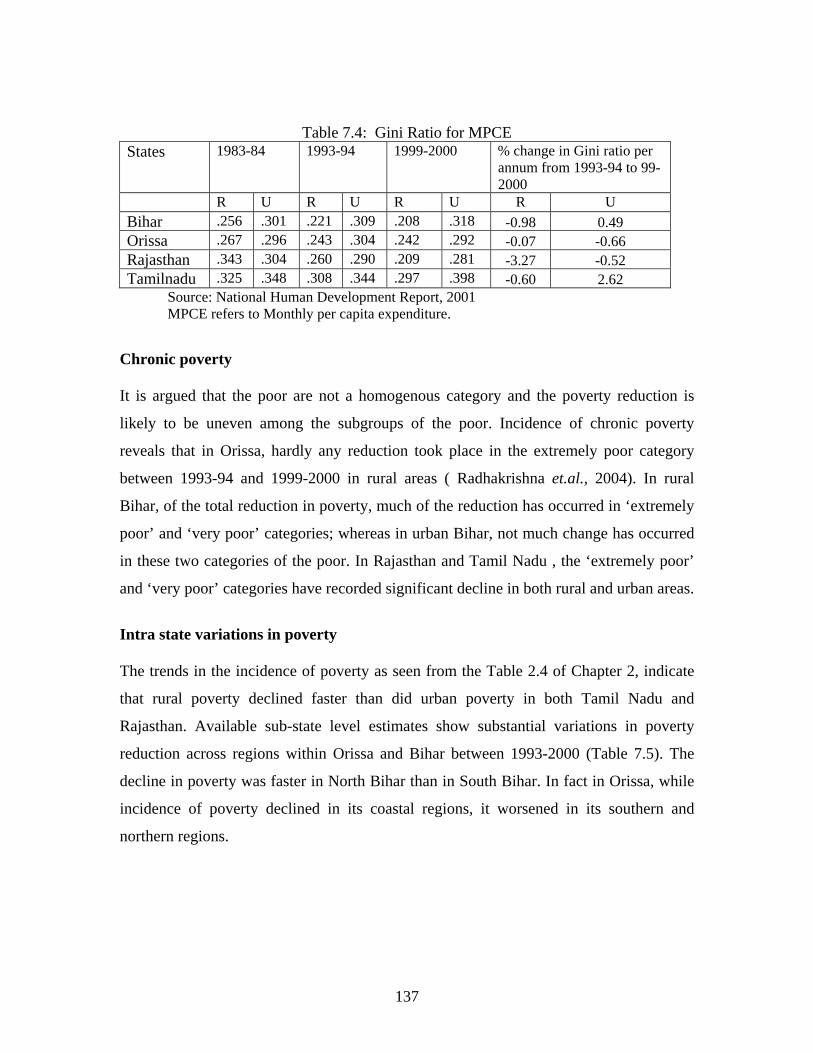
137

Table 7.4: Gini Ratio for MPCE States 1983-84 1993-94 1999-2000 % change in Gini ratio per

annum from 1993-94 to 99-2000

R U R U R U R U Bihar .256 .301 .221 .309 .208 .318 -0.98 0.49 Orissa .267 .296 .243 .304 .242 .292 -0.07 -0.66 Rajasthan .343 .304 .260 .290 .209 .281 -3.27 -0.52 Tamilnadu .325 .348 .308 .344 .297 .398 -0.60 2.62

Source: National Human Development Report, 2001 MPCE refers to Monthly per capita expenditure.

Chronic poverty It is argued that the poor are not a homogenous category and the poverty reduction is

likely to be uneven among the subgroups of the poor. Incidence of chronic poverty

reveals that in Orissa, hardly any reduction took place in the extremely poor category

between 1993-94 and 1999-2000 in rural areas ( Radhakrishna et.al., 2004). In rural

Bihar, of the total reduction in poverty, much of the reduction has occurred in ‘extremely

poor’ and ‘very poor’ categories; whereas in urban Bihar, not much change has occurred

in these two categories of the poor. In Rajasthan and Tamil Nadu , the ‘extremely poor’

and ‘very poor’ categories have recorded significant decline in both rural and urban areas.

Intra state variations in poverty The trends in the incidence of poverty as seen from the Table 2.4 of Chapter 2, indicate

that rural poverty declined faster than did urban poverty in both Tamil Nadu and

Rajasthan. Available sub-state level estimates show substantial variations in poverty

reduction across regions within Orissa and Bihar between 1993-2000 (Table 7.5). The

decline in poverty was faster in North Bihar than in South Bihar. In fact in Orissa, while

incidence of poverty declined in its coastal regions, it worsened in its southern and

northern regions.

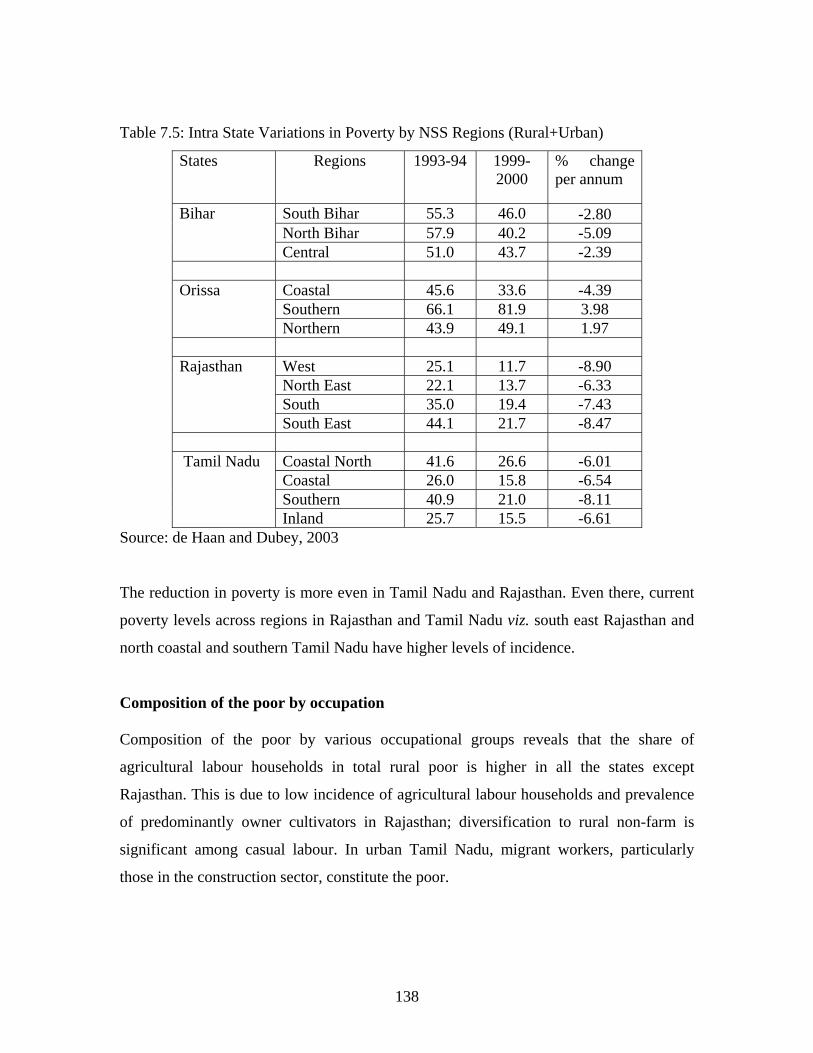
138

Table 7.5: Intra State Variations in Poverty by NSS Regions (Rural+Urban)

States

Regions 1993-94 1999-2000

% change per annum

South Bihar 55.3 46.0 -2.80 North Bihar 57.9 40.2 -5.09

Bihar

Central 51.0 43.7 -2.39

Coastal 45.6 33.6 -4.39 Southern 66.1 81.9 3.98

Orissa

Northern 43.9 49.1 1.97

West 25.1 11.7 -8.90 North East 22.1 13.7 -6.33 South 35.0 19.4 -7.43

Rajasthan

South East 44.1 21.7 -8.47

Coastal North 41.6 26.6 -6.01 Coastal 26.0 15.8 -6.54 Southern 40.9 21.0 -8.11

Tamil Nadu

Inland 25.7 15.5 -6.61 Source: de Haan and Dubey, 2003

The reduction in poverty is more even in Tamil Nadu and Rajasthan. Even there, current

poverty levels across regions in Rajasthan and Tamil Nadu viz. south east Rajasthan and

north coastal and southern Tamil Nadu have higher levels of incidence.

Composition of the poor by occupation Composition of the poor by various occupational groups reveals that the share of

agricultural labour households in total rural poor is higher in all the states except

Rajasthan. This is due to low incidence of agricultural labour households and prevalence

of predominantly owner cultivators in Rajasthan; diversification to rural non-farm is

significant among casual labour. In urban Tamil Nadu, migrant workers, particularly

those in the construction sector, constitute the poor.

139

Poverty by social groups Studies that analysed poverty incidence among social groups have shown that in India, a

ST household has 30% higher probability of being poor than other social groups. In

Orissa, 73% of STs were poor while 48% of the total population were poor in

1999-00. In fact, the disparity worsened between 1993-94 and 1999-00. Higher incidence

of poverty among the STs is associated with the depletion of forest resources. This has

been partly associated with the status of forest resources. Many poor tribals in Orissa,

who depend on non-timber forest product for livelihood have suffered over the last

decade owing to forest depletion and hence reduced availability of non-timber forest

products. There is a case of ‘entitlement failure’ also as there are reports that many tribal

lands have been acquired by non-tribals over time in Orissa (de Haan and Dubey, 2005).

In Tamil Nadu, poverty is concentrated among SC categories. Incidence of poverty in

1999-2000 among SCs was estimated at 32% in rural and 42% in urban. However, unlike

Orissa, the poverty levels among SCs have been declining over time. The reason

attributed to this decline is that, increasingly SCs are integrating with the mainstream

development process in Tamil Nadu. Effective implementation of reservation of jobs in

government and public sector and reservation in education, and historically certain social

movements fighting for socially downtrodden ( e.g. Periyar Movement) could be cited as

reasons for this phenomenon.

7.4 Human Development It has been emphasized that poverty as measured by income deficiency is not adequate to

capture full dimensions of human deprivation. A multi-dimensional approach, where

human development indicators such as education and health also play vital roles, is

helpful.

140

Table 7.6: Human Development Indicators

States 1981 1991 2001 Ranking based on poverty in 2001

HDI Rank HDI Rank HDI Rank Rank Bihar 0.237 15 0.308 15 0.367 15 14 Orissa 0.267 11 0.345 12 0.404 11 15 Rajasthan 0.256 12 0.347 11 0.424 9 6 Tamil Nadu

0.343 7 0.466 3 0.531 3 8

Source: National Human Development Report, 2001. Note: Only 15 major states for which data were available in 2001, have been ranked.

Tamil Nadu has made substantial progress in human development over the last two

decades. Its ranking on human development index is better than that in income poverty

criterion. In HDI, Tamil Nadu is among the top 3, while in income poverty it is in eighth

position. However, the state’s position in HDI could be cited as a reason for better

performance in income poverty reduction. The state’s emphasis on social policies and

programs partly explains this phenomenon. Orissa’s poor HDI matches its poor

performance in income poverty reduction. Rajasthan has performed much better in

achieving reduction in income poverty than in its progress in human development.

Perhaps, migration which augments income aggravates other deprivations especially

deprivation in education, health etc.

As regards education, Bihar has the lowest literacy rate among scheduled castes (Table

7.7). Orissa is next to Tamil Nadu in terms of female literacy and rural literacy. Even

though the enrollment rate has shown improvement, high drop out rates are reported in

Orissa. Reasons vary from financial constraints to lack of parental support and

uncongenial atmosphere in the schools. Substantial regional variation is reported in the

teacher-student ratio and the school infrastructure. Quality of literacy is also open to

question in many underdeveloped regions. Even though Rajasthan is improving its

position in literacy over time, it is still lagging behind in rural literacy and female

literacy. It is worth noting that rural literacy in Rajasthan has improved significantly from

27 % to 47% between 1991 and 2000. Innovative state specific programs initiated in the

recent periods underlie its progress.

141

Rural urban gap in literacy is narrowing down in all the states. However, Bihar

experiences larger rural-urban gap. Gender gap in literacy is the least in Tamil Nadu

among the four states. Moreover, Tamil Nadu’s record in the reduction of rural-urban

gap, from 30 percentage points in 1991 to 16 percentage points in 2001 is impressive. As

regards elementary education in this state, several initiatives taken by the state

government have helped to increase the enrolment rate. Tamil Nadu Compulsory

Elementary Education Act was passed in 1994. Moreover, other factors such as opening

of schools in close proximity to the habitation and implementation of supplementary

programs viz. free education to poor, noon meal scheme, free supply of text books and

uniform etc. improved its literacy status.

Table 7.7: Adult Literacy Rate

States Male Female Rural Urban Scheduled Caste

1991 2001 1991 2001 1991 2001 1991 2001 1991 2001 Bihar 50.30 59.68 18.47 33.12 30.35 43.92 67.89 71.93 19.49 40.23 Orissa 61.96 75.35 29.69 50.51 42.26 59.84 71.99 80.84 36.78 70.47 Rajasthan 52.54 75.70 16.89 43.85 26.91 55.34 65.33 76.20 26.29 68.99 Tamil Nadu

69.92 82.42 43.87 64.43 47.42 66.21 77.99 82.53 46.74 73.41

Source: National Human Development Report, 2001

Tamil Nadu is at the top of the ladder as regards infant mortality rate and life expectancy

at birth whereas Bihar is at the bottom of the ranking in terms of both the attributes. In

Bihar, almost all the health related development indicators are low as compared to all

India. Tamil Nadu has made rapid progress in health facilities as this is reflected in the

improved health indicators. The gender equality index has been improving over time

except for Bihar where it has declined during the eighties and the nineties. Tamil Nadu

has the highest gender equality index. There is large variation in this index among the

states as per 1991 data, from 0.469 in Bihar to 0.813 in Tamil Nadu. Total fertility rate

has been moving towards the norm of 2.0 in Tamil Nadu based on the data for the year

1997. Orissa comes next with a fertility rate of 3.0. In Bihar and Rajasthan, fertility rate is

higher, at around 4.3. Movement of demographic indices over time indicates that Tamil

Nadu is experiencing favorable demographic transition. The major contributory factor

seems to be female literacy. Women empowerment, which is reflected in higher gender

142

equality index, is an additional factor contributing to this process. Overall one can say

that economic growth along with public provisioning of education and health services

that ensure gender equality would lead to improvement in human development and

income poverty reduction as seen in Tamil Nadu.

Figure 7.2 Rural Literacy rate

0

10

20

30

40

50

60

70

1991 2001

BiharOrissaRajasthanTamil Nadu

7.5 Pattern of Income Growth Sectoral growth pattern indicates that, as expected, over time, tertiary sector is gaining

importance in all the states and the share of agriculture is coming down. Statistics on

income growth reveal that, Bihar, Tamil Nadu and Rajasthan have grown at an annual

rate of about 5% during 1993-94 to 2003-04 as compared to less than 4% for Orissa.

Higher growth of population has pulled down the per capita GSDP of Bihar, Orissa and

Rajasthan to a low of 2.2 – 2.3 percent per annum. On the other hand , Tamil Nadu could

achieve a per capita GSDP growth rate of 3.6 percent. The absolute per capita income is

much higher for Tamil Nadu , viz. 30% higher than that for Rajasthan.

Sectoral growth rates show the poor performance of agriculture in the 1990s in Bihar and

Orissa.; they registered an annual growth rate of -0.7 and 1.3 percent respectively (Table

7.8). Agriculture has fared better in Rajasthan and Tamil Nadu. Nevertheless its

performance has been less impressive than non-farm sector. Non-farm sector has grown

143

at an impressive rate of 7% to 8% per annum in the nineties in Tamil Nadu and

Rajasthan. Some of these favorable factors explain the faster poverty reduction in

Rajasthan and Tamil Nadu.

Table 7.8: Agriculture, Non-agriculture- Annual Real Income Growth (%) Poverty reduction per annum

States Agri. Growth between 1980-90

Agri growth between 1990-2000

Non-agri growth between 1980-90

Non-agri growth between 1990-2000 82-83 to

93-94 93-94 to

99-00Bihar 2.41 -0.71 6.18 3.90 -1.03 -3.75 Orissa 3.03 1.33 6.01 4.44 -2.12 -0.55 Rajasthan 3.06 3.50 8.06 8.17 -1.76 -7.68 Tamilnadu 3.28 2.92 5.40 7.33 -2.97 -6.61 Source: EPW Research Foundation

Growth rate indicates compound annual growth rate.

Non-farm sector is an important source of income and employment for rural households

in Tamil Nadu and Rajasthan. This is attributed to rapid expansion of rural infrastructure

facilities, especially road networks that have facilitated migration even from remote

areas. In Rajasthan, development of mining and quarrying activities in rural areas has

generated substantial income and employment. In Tamil Nadu, textile sector plays a

major role in providing employment in rural areas next only to agriculture and

contributes substantially to the state’s economy. Its share in the export of yarn is 40% of

cotton valued at Rs.2500 crores as against the country’s total export of Rs.6,320 crores.

The knitting and hosiery industry located in Tirupur , derives importance from its export

potential. More than 9000 small scale units are functioning in this cluster. The industrial

cluster has experienced tremendous growth in the last two decades. With the total

turnover of Rs. 9,500 crores of which export is Rs. 4,500 crores, Tirupur accounts for

56% of the country’s export in that sector. In employment, women account for about 60%

of the total work force in Tirupur textiles sector. Bihar and Orissa have not made much

progress in the non–farm sector. In Bihar, allied agricultural sector seems to have better

growth potential. In recent period, fisheries, dairy and horticulture (especially litchi and

banana) have been showing promising growth in Bihar. A substantial portion of state

144

income comes from these three sectors. Bihar has a comparative advantage in horticulture

and fishery because of its rich alluvial soil and hydro resources.

Based on the study made by Ravallion and Datt (2002) that associates growth of non-

farm output with poverty using the NSSO data from 1960-61 to 1993-94, it can be

inferred that (Table 7.9), the poverty reducing effect of non-farm growth is weak in

Bihar. In the case of other states, a 1% increase in non-farm per capita income reduces

incidence of poverty measured by HCR by half a percent. Ravallion and Datt showed that

the poverty reducing effect of non-farm growth would depend on initial conditions such

as incidence of landless rural population, share of urban population, infant mortality rate,

female literacy rate etc. According to them, in states like Bihar, unfavourable initial

conditions inhibit the prospect of poor participating in the growth prospects of non-farm

sector.

Table 7.9: Elasticity of Poverty with respect to Real Non -farm Output per capita (Period of study 1960-61 to 1993-94)

Elasticities States

HCR PG SPG Per capita Non farm Growth

Bihar -0.26 -0.67 -1.00 1.96 Orissa -0.66 -1.06 -1.40 3.15 Rajasthan -0.66 -0.98 -1.20 2.41 Tamil Nadu -0.56 -0.80 -0.96 3.88

Source: Ravallion and Datt, 2002 In the rural areas, land is the most important asset that influences the livelihood of the

people. The asset distribution, especially land, can throw some light on the structural

variations in different states. It is widely known that in Bihar and Orissa agrarian

relations are less conducive to poverty reduction. Structural rigidities and insecurity of

land tenure have inhibited agricultural growth as well as poverty reduction. Adoption of

modern technology among small and middle farmers is very low in both Bihar and

Orissa. It could also be due to lack of effective extension and demonstration programs in

these states. As against this, structural transformation has taken place in Tamil Nadu

owing to social movements as well as reforms undertaken by the state. Small farmers are

able to adopt modern technologies helped by a well-designed and implemented extension

145

and training programs. This state has recorded impressive growth in foodgrain

productivity over the last two decades. Estimates of output value per hectare for the NSS

regions during the year 1999-2000 show that it was in the range of Rs. 4,000 to Rs. 7,000

in 1990-93 prices in all the selected states except Tamil Nadu (Himanshu, 2005). In

Tamil Nadu, it was as high as Rs. 20,000 (Table 7.2). Output per worker also reflects a

similar pattern. Higher agricultural growth and a somewhat stronger association between

poverty and per capita agricultural income are some of the favourable factors underlying

rural poverty reduction in Tamil Nadu (Table 7.10)

Table 7.10: Elasticity of Poverty with respect to Agricultural Income per capita

(Period of Analysis 1960-61 to 1999-2000)

Elasticities States

Per capita agricultural

income growth

HCR PG SPG

Bihar 1.31 -0.412 -1.075 -1.609

Orissa 1.88 -0.355 -0.674 -0.998 Rajasthan 1.52 -0.485 -0.749 -0.950 Tamil Nadu

2.96 -0.700 -1.213 -1.617

Source: Panda, 2003.

There is no significant shift to commercial crops from subsistence crops over the years in

Bihar as the share of area under foodgrains to gross cropped area is as high as 90% as

against the share of 50% to 60% in other states. Subsistence concern and rigidity in

practices mostly explain absence of any major shift towards non-foodgrains. In recent

years, Bihar has been witnessing a spurt in the growth of horticulture. Crops like lichi

and banana are emerging as engines of growth. However, their overall impact on poverty

seems to be marginal. The allied sectors like animal husbandry and fishing have

performed reasonably well in Bihar. Both horticulture and animal husbandry sectors hold

the future for Bihar.

Notable shifts towards oilseeds and fiber crops have taken place in Rajasthan. It has seen

significant crop diversification and agricultural growth in crop productivity in arid and

rainfed areas. Development of markets and increase in productivity are cited as factors

146

underlying the above changes. The poverty reducing effect of diversification has however

been little researched. The impact of diversification on poverty would depend on the

extent to which new technologies are accessible to small farmers and the extent to which

small farmers are equipped with marketing skills.

Diversification to non-farm and intersectoral linkages Diversification of income earning activities helps to reduce risk associated with a single

source of income from farming. Rajasthan shows increased diversification in rural areas.

This is particularly seen in income generating potential of the livestock sector in

Rajasthan. Tourism in Rajasthan, as is widely known, boosts the state economy; and it

also helps growth of other sectors through sectoral linkages. Artisanary and handicrafts

also contribute to the diversity of the state’s economic activities. Better performance of

the non-agriculture sector and its strong linkages with agricultural sector, have enabled

Tamil Nadu to record significant poverty reduction in both rural and urban areas. Studies

on intersectoral linkages (e.g. Kalirajan and Sankar, 2001) have found empirical

evidences for the fact that in Tamil Nadu and Orissa, there is a bi-directional linkage

between agriculture and industry implying that the growth in farm sector triggers off

growth in industry and vice-versa. Whereas in Rajasthan and Bihar it is unidirectional

with Rajasthan showing the tendency for sectoral flows to move from industry to

agriculture and in Bihar it is from agriculture to industry.

7.6 Employment Scenario Employment data reveal that overall there was a slowdown in the growth of employment

in the nineties as compared to the eighties. The annual growth of employment has

dropped in all the states except in Bihar. The slowdown may be partly attributed to

withdrawal of child labour from the labour market. On the other hand, there may be

voluntary withdrawal of youth labour also. If the withdrawal of youth labour is for the

sake of human capital building then it is voluntary. Such reduction in employment should

be treated as a welcome factor. Shifts of labour from primary agricultural sector to more

147

productive industries and service sectors were witnessed over time in the 70s and 80s.

But this trend has slowed down in the nineties and after.

Casualisation of labour has occurred over time in all the states. Volatility in labour

market exposes the vulnerable and the poor to labour market risks. The resultant

casualisation of labour is one factor that increases vulnerability of the poor to labour

market risks. Even though manufacturing and service sectors have achieved impressive

growth in employment, still owing to their small share of total employment, they have not

contributed much to the otherwise declining employment.

Employment scenario is not encouraging even in the better performing state of Tamil

Nadu. About 90% of its workforce is in the unorganized sector. Incidence of

unemployment is far higher in Tamil Nadu than in other states (Table 7.11). Particularly,

unemployment among educated youth is widespread. Bihar and Orissa have lower

incidence of unemployment than Tamil Nadu. It is difficult to bring out any association

between unemployment and poverty at the aggregate level between different regions or

between states; however at the household level, unemployment does increase the risk of

poverty. Rajasthan has low level of unemployment. It could be due to its diversified

employment opportunities. Mining activities in the arid and semi arid regions might have

provided livelihood opportunities to the poor. About 50% of the work force employed in

mining comes from SC and ST communities.

Table 7.11: Incidence of Unemployment (per 1000 days on CDS basis) -Rural

Source: NSSO, various rounds Note: CDS refers to ‘current daily status’

Net migration is one factor that would reduce the supply of labour and hence put pressure

on local wages. In Rajasthan, migration has taken place regardless of income status of the

household. Both rich and poor have resorted to migration. Migration from rural to urban

area has worked in favour of the rural poor, by pushing up real wages. An interesting

States Male Female 93-94 99-2000 93-94 99-20 00 Bihar 63 46 72 62 Orissa 76 51 76 56 Rajasthan 15 4 33 19 Tamilnadu 128 113 143 123

148

aspect of migration in Bihar is, increasingly more and more upper caste persons migrate

because they are not able to break caste taboos against manual wage work in their

villages. Lower castes migrate to avoid falling victims to the prevailing system of caste

discrimination in the village.

Inter and intra state variations in the incidence of unemployment, extent of casualisation,

relative size of non farm sector etc. are significant (Table 7.12). Proportion of casual

workers is very high in all regions of Tamil Nadu, 50-55% as compared to 12-27% in

Rajasthan. Wage levels are higher in Tamil Nadu followed by Rajasthan.

Table 7.12: Key Employment Statistics for the NSS Regions - Rural 1999-00

States

Regions Workforce participation

rate-

Usual status

Unemployment rate - Usual status

adjusted

% employed

in non farm sector- Usual status

% employed as casual workers- Usual status

Non farm wage Rs.

Southern Bihar

37.5

31 27..0

32.9

41

North Bihar

31.3 15 15.8

51.0 50

Bihar

Central 34.9 11 18.3 43.5 43

Coastal 34.4 39 28.2 38.8 42 Southern 50.8 3 11.2 56.4 40

Orissa

Northern 47.8 11 22.3 49.2 38

West 44.1 6 16.9 13.4 62 North East

41.9 4 24.6

11.6 61

Southern 49.1 1 32.8 26.6 55

Rajasthan

South Eastern

49.7

3 17.3

16.7

55

Coastal North

46.8

27 31.5

50.2

70

Coastal 50.5 16 23.3 56.9 66 Southern 53.1 23 34.4 50.7 69

Tamil Nadu

Inland 55.7 12 37.2 49.4 116 Source: Himanshu, 2005

149

The fast growing Tamil Nadu and Rajasthan had witnessed slower employment growth

between 1993-94 and 1999-00 (Table 7.13). The implicit employment elasticity is

estimated to be lower for Tamil Nadu and Rajasthan. Higher wages and lower population

growth in Tamil Nadu and moderately higher wages and higher incidence of migration

might have contributed to their good performance in poverty reduction despite their poor

performance in employment growth.

Table 7.13: Annual Employment Growth compared with GDP Growth and

Employment Elasticity of GDP -between 1993-94 and 1999-2000 States

Employment growth

GDP growth

Employment elasticity of GDP

Poverty decline per annum from 93-94 to 99-2000

Bihar 1.59 4.5 0.353 -3.75 Orissa 1.05 4.0 0.262 -0.55 Rajasthan 0.73 7.0 0.104 -7.68 Tamil Nadu 0.37 7.1 0.052 -6.61

Source: Economic Survey

Real wage for unskilled agricultural labour has improved during 1993-1999 at an annual

average of 8.15% in Tamil Nadu, 3.89% in Rajasthan and 0.98% in Bihar while it has

declined in Orissa (Table 7.14). The performance of a state in poverty reduction is by and

large in consonance with its improvement in real wage. The agricultural wage rates in

Tamil Nadu and Rajasthan are significantly higher than that in Bihar and Orissa. The

average daily wage for casual labour in agriculture in 2003-04 was about Rs.50 in Bihar

and Orissa, whereas it was about Rs. 80 in Rajasthan and Tamil Nadu. Sizable rural–

urban migration has raised the agricultural wage in Tamil Nadu and Rajasthan and this

has contributed to reduction in rural poverty. In fact even when the per capita agricultural

income was stagnant in the nineties, improvement in the agricultural wage was sustained.

Non-farm wage classified according to NSS regions showed significant regional variation

in Tamil Nadu (Table 7.12). In ‘Inland’ it was twice that of other regions in the 1990s.

150

Table 7.14: Annual Percentage Change in Real wages

for unskilled Agricultural Labour States % change over previous year

93-94 94-95 95-96 96-97 97-98 98-99 99-2000

Average % change per annum

Average daily wage 2003- in Agriculture Rs.

Bihar 5.98 1.69 -2.3 15.15 -4.7 -5.7 -3.26 0.98 53

Orissa -0.14 -3.52 0.55 -0.41 2.39 0.61 -0.23 -0.11 50 Rajasthan -7.66 1.05 10.33 17.81 5.12 -16.26 16.83 3.89 77 Tamil Nadu

11.60 1.03 3.63 7.90 13.39 2.63 16.84 8.15 80

Source: Economic Survey

Figure 7.3 Percentage Growth in Real Agricultural Wages

-6

-4

-2

0

2

4

6

8

10

1987-88 to 93-94 1993-94 to 99-00

BiharOrissaRajasthanTamil Nadu

7.7 Infrastructure Infrastructural development is the backbone of rural development and it is expected to

distribute the gains from agriculture widely by providing opportunities to less developed

regions and to small and marginal farmers. Studies relating infrastructural development

and rural poverty have found that factors like irrigation, rural electrification and roads not

only improve agriculture growth and but also have favourable distributional impact. A

study by Hanumantha Rao et al. (1986) using data on NSS regions has provided

151

empirical evidence to the view that development of irrigation and rural electrification is

associated with lower poverty ratio. Benefits from canal irrigation, particularly seem to

have a favorable distributional impact on different classes of farmers. A study by Fan

Shenggen et al. (2000) has found that, improved road networks reduce poverty by way of

higher wages and non-farm employment. This study has also concluded that a marginal

rupee spent on rural roads has a larger impact on poverty than the other government

spending.

Infrastructure in Tamil Nadu has expanded faster in the last two decades and it is

comparatively better than the other states in terms of the composite index. Road density

per 100 sq. km. of geographical area, as of 1999 was lower in Rajasthan and Bihar with

41.20 Km. and 51.40 Km. respectively; for Orissa, it was 168.60 km; and Tamil Nadu,

117.70 Km. Bihar has witnessed very little growth in road network in the last four

decades. The annual percentage increase in road length between 1960 and 1999 was

estimated at 0.26% for Bihar. The corresponding figures for the other states are 19%,

6.4% and 5.6% respectively for Orissa, Rajasthan and Tamil Nadu.

Irrigation

The poverty reducing effect of access to irrigation has been firmly established (Table 3.6,

Chapter 3). In Orissa and Bihar incidence of poverty among households with no

possession of irrigated land is twice that of those with irrigated land; in Tamil Nadu,

poverty incidence is 40% higher among the households with no irrigation facility and in

Rajasthan, it is about 15% higher.

Irrigation shows substantial variations across regions especially in Bihar and Rajasthan

(Table 7.2). Irrigated area has recorded faster rate of utilization in Tamil Nadu. It has

exhausted all the potential in major irrigation surface water and very little stock is left in

minor irrigation. Ground water also is being overexploited in this state. All these factors

go to show that sustaining the growth in agriculture is difficult in the future. Fast growth

of agriculture has also brought with it extensive degradation in Tamil Nadu. Percentage

of water logged and saline area to total geographical area is 2.23 for Tamil Nadu as

against less than 1% for other states.

152

Even though Bihar is well endowed with water resources, it is constrained by inefficient

management of drainage, floods and droughts and poor water management. Incorrect

pricing and distributional inefficiency of public irrigation add to the problem. In Orissa,

of the total irrigation potential generated, 53% comes from minor (flow and lift) and

other sources. Due to erratic behaviour of monsoon and scanty rainfall, major parts of

minor irrigation projects fail to provide required water on time. Besides this, constraints

in the supply of electricity have contributed to uneven distribution and poor performance

of irrigation use in Orissa. In Rajasthan, due to its meager water resources, the state has

made concerted efforts to expand irrigated area during the last four decades. Over 70% of

irrigation depends on ground water.

Financial infrastructure Bihar lags behind in terms of financial infrastructure. In 2003, there was only one

scheduled commercial bank per one lakh population as compared to one per 26000

persons in Tamil Nadu. The credit deposit ratio was 24 as compared to the maximum of

93, in Tamil Nadu. Investment climate is not conducive in Bihar and is subject to a higher

degree of risk. In the wake of emphasis upon more prudential norms after the initiation of

reforms in nineties, banks put a brake on the growth of priority sector lending. The inter-

regional pattern of credit-deposit ratio was very disturbing in late nineties. For instance,

between 1991 and 2001, CDR in rural areas declined from 57.5% to 21.2%. This decline

is far higher than the reduction in semi urban or urban areas. In per capita terms, private

and public investment, plan outlay, institutional investment and total credit utilized all

were lower for Bihar in 2000-01. Data on institutional lending through different sources

indicates that SCBs dominate over cooperatives in Bihar (Table 7.15). This is true even

in the case of marginal and small farmers. The capital formation per capita is also one of

the lowest for Bihar. The FDI is also low. This impinges on the growth potential due to

inadequate capital for undertaking necessary infrastructure development.

153

Table 7.15: Proportion of Institutional Credit by Farm Size Categories

- for the year 2005

Proportion of Institutional Credit available through

Sub-marginal

farms

Marginal

farms

Small farms Medium

farms

Large

farms

States

SCB Coops SCB Co

ops

SCB Co

ops

SCB Co

ops

SCB Co

ops

Bihar 89.9 6.2 84.7 5.7 91.2 8.1 88.2 1.4 93.4 6.6

Orissa 71.5 22.0 58.5 18.7 46.5 28.8 59.8 37.7 63.4 36.6

Rajasthan 72.0 23.7 64.3 23.2 82.7 16.1 85.0 12.5 72.3 23.4

Tamil

Nadu

47.4 48.5 44.3 51.1 58.7 38.2 44.5 49.8 71.1 28.5

Source: Rangarajan, 2006

Orissa also presents a dismal picture. In 2003, it had one bank per lakh population. CDR

has declined from 70% in nineties to 41.5% in 2001. Since access to formal credit

market is low, informal credit is the main source of credit in rural areas. The climate is

not conducive to new investment in agriculture. Micro credit, which has made a

beginning in Orissa is yet to expand in scale.

Financial institutions in rural Rajasthan mostly comprise Scheduled Commercial Banks

(SCBs) , Regional Rural Banks and Cooperatives. The share of rural branches of SCBs

declined from 66% to 56% between 1991 and 2001. As a result, population coverage per

branch has gone up. This trend is attributed to the policy shifts that resulted in the merger

of loss-making rural branches with the profit making branches. In this state, the gap

between deposit mobilization and credit deployment in rural areas of the state has

increased during the reforms period. Of the total credit disbursement, the share of PACs

is only 24%. Of the total credit to small farmers and marginal farmers, the share of PAC

is below 25%. Inequality has increased in the disbursement of production credit from

PACs. The reason attributed to this is large number of defaults from small farmers and

their subsequent loss of access to credit. However, innovation in institutional credit, for

154

e.g micro finance contributed to poverty reduction. In term lending by SCBs, the number

of beneficiaries of small and marginal farmers declined from 63% during triennium

ending 1987-88 to 56% during triennium ending 1997-98. Corresponding share in credit

disbursal declined from 24.5% to 20.4%. The Cooperatives and the SCBs are functioning

with greater efficiency. The performance of the Cooperatives and SCBs in terms of

recovery and the business handled per staff is significantly higher than the all India

average.

Tamil Nadu is well placed in terms of the spread of bank branches and physical

accessibility. Banks are more evenly distributed between rural and urban areas. As

mentioned earlier, in terms of number of bank branches, it accounts for 7% of the total

number of branches in the country. Credit deposit ratio is also quite impressive.

Cumulative farm credit per hectare in 2002 is was Rs. 2,200 in Tamil Nadu, much higher

than for other states, where it is in the range of Rs.200 to Rs. 300. Besides commercial

banks, the network of about 4600 primary agricultural cooperative banks (PACB) at the

village level provides short term and medium term loans to the farmers. There is a three-

tier cooperative structure with State Co-Operative Bank at apex level and District

cooperative Banks at the middle level and PACBs at the grass root level, which extend

credit facilities to the farmers.

7.8 Fiscal Scenario The fiscal crisis of Bihar state brought on by the inability of the state to mobilize

resources internally resulted in low budget allocation for poverty alleviation programs.

Per capita real social expenditure witnessed a 23% decline from the early 90s to early

2000 (Table 4.7, Chapter 4). Outlay on social sector as a percentage of total spending has

also declined by about 10% during this period. The share of budgetary resources going to

education sector has witnessed a large decline. Stagnant tax and non-tax revenues

coupled with an increase in salaries of the staff as a result of the Fifth Pay Commission

recommendation, has compounded the fiscal crisis. Political expediency has triumphed

over economic rationale in many instances. Mounting fiscal deficits and widening

revenue expenditure gaps have forced the State to take recourse to high interest cost

borrowing, thus leading to very low plan capital outlay in the case of Bihar. All these

155

factors have restricted ability of the State to undertake investments in social and

economic infrastructure. Fiscal reforms are needed especially to tone up revenue by way

of simplifying the tax system, making the administration more accountable and

improving the level of cooperation between different tax departments. Growth of non-tax

revenue and public sector reforms are crucial to improve the fiscal position.

Per capita real public expenditure in social sector has gone up between 1990 and 2000 in

Orissa. Budget outlay on social sector as a proportion of total spending has increased

marginally between 1990 and 2000. The increase has mainly gone to education sector. In

the health sector, the share has declined from 3.6% in 90-91 to 2.5% in 2001-02. Orissa is

passing through a severe fiscal crisis. It moved from a revenue surplus state in 1980-81 to

revenue deficit state in the 1990s. About 80% of state’s own revenue and 34% of its total

revenue inclusive of shared taxes and grant-in-aid accounting for 6.5% of SDP are being

used for debt servicing. A major proportion of the plan revenue expenditure and a part of

the non-plan expenditure are being funded from the receipts on capital account. What is

worse, revenue expenditure is growing at the cost of capital expenditure. Governance

reform is considered to be the solution to the current fiscal crisis. The state has launched

a fiscal and governance reform programs. Various measures have been undertaken to

increase tax and non-tax revenue and public sector restructuring and debt restructuring.

However, there are problems in their implementation. Power sector reforms have not

yielded desired results due to unsatisfactory functioning of Electricity Regulatory

Commission in the State. Some of the reform measures have been reversed. Similar is the

fate of water resource management reforms. Given the fiscal condition of the state, steps

are needed to attract private investment to finance infrastructure development. Recently

the state has signed MOU for private sector establishments in the steel sector. This will

boost Orissa’s industrial production and the state economy provided governance

improves considerably.

In Rajasthan, per capita real expenditure on social sector has gone up by 55% between

1990 and 2000. Fiscal situation worsened in the nineties and to overcome this, fiscal

reforms were initiated starting with agriculture and power sector. However, they were

inadequate to overhaul fiscal situation. Plan financing is constrained by extreme paucity

of funds. The return on investment is very low. This makes fiscal situation unsustainable

156

as investments are funded from borrowings at high rate of interest. Panchayat Raj

institutions are very weak in Rajasthan. This is attributed to low literacy rates and

inadequate knowledge of the functions of the institutions among the elected

representatives on the one hand and lack of own resources on the other. An improvement

in the quality of representation would help to improve PRI governance. Budget outlay on

social sector as a percentage of total spending has witnessed a marginal increase of 4

percentage points. Increasing share in education and a decreasing share in health are

observed. The share of medical and health services in the total spending went down from

7.2% in 1990-91 to 5.8% in 2000-01.

In the per capita real social service expenditure, Tamil Nadu has registered a 40%

increase between 1990 and 2000. The funds allocated to social sector as a percentage of

total spending has seen a 10% points decline. The share of education went down from

22% in 1990-91 to 17.8% in 2000-01 and from 6.6% to 5% for health sector. Food

subsidy accounted for less than 1% of the total expenditure in 1980-81; by 2000-01 it

emerged as a major item of expenditure accounting for 6.5% of total spending. The

absolute expenditure on nutrition programs has almost doubled between 1990s and 2000;

though as a percentage of total spending, it has gone down from 4% to 2.27% in the same

period. Budgetary allocation to poverty alleviation programs has declined from 5.5% to

3.5% of total outlay between 1990-91 and 2000-01. Even though availability of good

infrastructure, quality manpower and the “investor friendly” approach adopted by Tamil

Nadu have attracted considerable private investment especially foreign direct investment

(FDI) into the State during Eighth and Ninth Plan, the finances of the State began to

deteriorate during the later half of nineties. Responding to the fiscal crisis, the state

implemented during 2002-03, a number of corrective actions encompassing revenue

augmentation, expenditure reduction, power sector reforms and accommodating more

private sector investment. However the state did not continue with these efforts with

vigour. After the electoral debacle of the ruling party in the parliamentary elections, the

state suffered a setback in reform measures. Meanwhile a large number of reputed

software firms have shown willingness to invest in Tamil Nadu. The state has taken up

the opportunity and created a conducive environment for IT development. The export

157

intensive sectors, especially textiles, have registered significant growth. Modernisation of

textiles is one important reason why this sector is able to withstand competition.

7.9 Determinants of Poverty: An empirical exercise

Regression analysis is carried out to explain the inter district variations in poverty

during the year 1999-2000. The data on relevant variables have been extracted from

NSSO and the CMIE, District Statistics. Totally 82 districts from the four states

constitute the sample. Three alternative measures of poverty have been tried as dependent

variable and the results are presented in Table 7.16. All the variables are included in

logarithmic form. All the coefficients possess correct signs. However, agricultural

income per capita in rural areas is not statistically significant in explaining the inter-

district variations in poverty. It can be observed from the table, rural literacy rate is the

dominant factor of all. The size of land holding is the next important variable explaining

rural poverty reduction.

The results show that rural literacy is the most important factor to be targeted for

reducing rural poverty. Shift variables for the states have also been considered and found

to be significant. The signs of the state dummy coefficients suggest that the base poverty

level is lower in the other states than in Orissa. State dummy coefficients imply that given

the level of explanatory variables same in all the states, there are still variations in the

poverty status due to variations in initial endowments and other institutional and policy

variables9.

9 The specification could be improved by adding infrastructure variables, both physical and financial, and other human development indicators. Preliminary trials with some of these variables did not yield expected results. Due to lack of data, a crucial variable like wage rate was not included.

158

Table 7.16: Elasticity of Rural Poverty with respect to various Characteristics10 Variables Head

count ratio

Poverty gap

Squared poverty gap

Elasticity Rural literacy rate -0.887* -0.928*

-1.076*

Agriculture income per capita rural

-0.172

-0.207

-0.203

Average holding Size#

-0.613*

-0.729*

-0.879*

R2 0.561* 0.621* 0.615* Sample size 82

# Average holding size is computed as the ratio of total land cultivated to the total number of farmers. *significant at 5% level.

7.10 Programs of Poverty Alleviation Regardless of the initial conditions of endowment and distribution, government targeted

programs are expected to give necessary fillip directly for the poor to improve their

economic status. There are various centrally sponsored schemes common to all the states

and state specific programs for poverty alleviation. Common central programs are mainly

self-employment programs, wage employment programs, food and nutrition programs

and social security related programs.

Performances vary among the states for common programs because of initial conditions

and the way implementation process is carried on. In Bihar, a comprehensive self-

employment program started in April, 1999 has replaced various components under this

scheme. But the evaluation studies have shown that it has not made much impact. Among

the wage employment programs, Employment Assurance Scheme, which helps the rural

poor in lean agricultural season, has gradually covered more and more blocks and in

10 The system of equations were tested for simultaneous bias by performing endogeneity test (Durbin- Wu- Hausman test) . The simultaneous problem might occur because agriculture income per capita could be endogenous in the system. However the test has proved that there is no simultaneous bias in the specification.

159

terms of desired targets this program has performed well with the achievement rate of

above 90%. As regards PDS, in Bihar, where food production per capita is low, PDS is

expected to help the poor in meeting their food needs. But, on the contrary, the PDS

allocation and offtake have been very low. Poor delivery system is the main cause. Large

level of leakages has been reported. Political commitment is needed to bring in reforms to

make PDS to contribute to the overall reduction in poverty. In this state, programs that

lead to the organization of self-help groups, have not progressed as expected due to very

low ‘ground level credit flow’.

In Bihar, one of the major factors underlying the poor performance of poverty alleviation

programs and lack of political commitments is due to its backward agrarian structure.

Some legislation pertaining to land reforms viz. Land Ceiling and Tenancy Acts were

grossly violated because of inadequate implementation. Programs that provide basic

infrastructure and basic civic amenities for better quality of life in rural areas also are

weak.

In Orissa, the employment generation schemes consist of provision of employment to the

unskilled workers and the state has mandated that 30% of the total employment

generation should reach women. The targets of wage employment programs have not

been met in most years. Self-employment programs are reportedly suffering from poor

and inefficient credit delivery. Orissa also reveals failure of PDS to cater for the food

needs of the poor adequately. Many constraints such as communication gap between

ration shops and the buyers about the exact time of arrival and lack of cash on the part of

buyersat the time of arrival etc. are cited for poor offtake from PDS. The supplementary

food distribution through Annapurna Scheme has also faced similar problems. It needs to

be noted however that in the cyclone year 1999-00, PDS performed well. The ICDS

scheme has made significant impact. Provision of noon meal to school going children has

improved the attendance rate ovarall, among SC/STs and girl children. However, there is

lack of coordination between this scheme and other nutrition programs at the grass roots

level. The state is trying to improve the primary school enrollment through District

Primary Education program. The progress is slow however, thanks to organizational

problems and paucity of funds. Participatory water management is one scheme that is

intended to improve soil and water management in the rural areas. The state had formed

160

Water Shed Mission in 2000-01 with a view to ensuring soil and water conservation. In

order to facilitate the process of participatory water management the state passed Pani

Panchayat Act in 2002. Micro evidence shows that PPs are not democratic and the rich

and the elites control most of the decisions relating to maintenance and distribution of

water. Overall in Orissa, many programs suffer from poor functioning and absence of

community participation. The coverage of the state run old age pension scheme is very

small and hence has had little impact.

In Rajasthan, some innovative schemes for rural infrastructure development and micro

credit finance have proved successful in the recent period. However, asset redistributive

programs such as IRDP and income transfer programs, and PDS have been efficiently

carried out. These programs are not very successful as far as poverty reduction is

concerned. Employment programs in the state depend on the drought intensity. Growth,

both in the farm and non-farm sector, and rapid development of rural infrastructure,

facilitating migration even from the remote areas, might explain poverty reduction in the

state better than the directly targeting programs. However some state specific programs

and administrative reforms have been successful. One of the administrative reforms is the

enactment of Right to Information. This has improved the accountability of programs and

better transparency thereby has helped the effective implementation of the programs.

Public hearing of the grievances in the welfare programs is a specific feature, that has

helped benefit of the programs to reach the targeted people with less corruption.

In Tamil Nadu, social policies, notably the one relating to reservation of jobs in

government and state public sector undertakings and reservation of seats in educational

institutions including higher and professional education based on social class, as well as

integration of socially excluded communities with the mainstream have played a vital

role in the reduction of poverty. Government’s direct interventions put emphasis on

provision of basic minimum services. Tamil Nadu’s efforts in improving the nutritional

status of its population through innovative schemes with strong political commitment for

effective implementation have received universal acclaim (Box 7.1). A few of the

schemes, notably the School Noon Meal Scheme, have been expanded nationwide.

Started in 1956 as mid day meal scheme, it launched its World Bank supported Tamil

Nadu Integrated Nutrition Project (TINIP) in 1980. This scheme provides supplementary

161

nutrition to children under 3 years age and educates women on breast feeding, weaning

and growth monitoring.

A unique feature of PDS in Tamil Nadu is its universal coverage. A large network of fair

price shops and arrangement with the neighboring states for inflow of foodgrains during

shortfall, have helped to keep grain prices low even during drought season. Higher level

of internal procurement of paddy to maintain the supply is an additional feature. It is

reported that monthly purchases from PDS is higher in Tamil Nadu than in many other

states. The state’s policy of maintaining the issue price below the central issue price has

provided income gain to the poor. Income gain per capita from PDS shown in Table 7.17

reveals that Tamil Nadu has provided more benefits to the poor thorough PDS than other

states. It is also shown that Orissa has been improving in PDS delivery system and it

benefits the poor more compared with Bihar and Rajasthan.

There are other programs such as ‘Pension to the old people, destitute and physically

handicapped’. Tamil Nadu’s success has been the outcome of effective implementation of

programs, that enable the poor to participate in the democratic process. As reported

earlier, textile sector is one of the major sectors generating both employment and income

in the state.

Table 7.17: Per Capita Income Gain (Rs. Per month) from PDS in Rural Areas 1999-2000

States to Poor to Non-poor Cereals All-

commodities Cereals All commodities

Bihar 0.80 4.08 2.11 5.12 Orissa 10.02 11.44 7.79 10.53 Rajasthan 0.56 3.71 0.45 3.65 Tamil Nadu 20.28 32.80 25.49 32.80

Source: Sambi Reddy and Hanumantha Rao, 2004

162

Box 7.1: Nutrition Program in Tamil Nadu Nutritious Meal Program ( NMP) has been formulated by the government of Tamil Nadu to improve the health and nutritional status of children and to develop their mental and physical capability by direct provision of food and food supplements. Launched in July, 1982, initially, this scheme covered rural pre-school children in the age group 2-5 years through the network of noon meal centers. Subsequently the scheme was extended to urban pre schoolers also. In 1984, the program was further expanded to cover the school students of 10 to 15 years of age. In 1983, the old age pensioners were made eligible under the program. From December 1995, pregnant women have also been included under the program to enjoy the benefits for 4 months during the period of pregnancy. Overall there are more than 70000 noon meal centers feeding over 77 lakhs children and 5 lakh adults. Besides improving nutritional status of children, these schemes also serve as incentives for increasing the enrollment in and reducing dropouts from schools. While initially the noon meal programs were started to combat hunger and malnutrition, over the years the state government has taken initiative to combine provision of food with other services like health care, immunization, growth monitoring, pre and post natal care for women, communication and nutrition education. In 1994, a State Policy on Nutrition was explicitly drafted with technical support from the UNICEF. The state has been spending significantly on the NMP. Budgetary allocation to NMP has increased from Rs. 27,230 lakhs in 1992-93 to Rs.58,118 lakhs in 2000-01. As a percentage to total social service expenditure, it ranged from 6.5% to 7.8% during the same period. Expenditure on the ‘nutrition’ head ranks third after ‘education’ and ‘medical and public health’. Impressed by the success of the nutrition programs in Tamil Nadu , Government of India supported similar initiatives in the other states. The impact of the nutrition programs has been well documented. Based on the evaluation reports of National Institute of Nutrition, in Tamil Nadu, distribution of 1-5 aged group children by nutritional status between 1975 and 1996 showed that the percentage of children with normal nutritional status increased from 6.2 % to 14.4% during this period; that of mildly mal nourished from 34.2% to 49.2%; incidence of severely malnourished children declined from 14.4% to a low 2.9%. The percentage decline of malnourished is much sharper than the all –India figures. Source: Social Welfare and Nutritious Meal Programme Department, Government of

Tamil Nadu, Policy Note -2005-2006.

163

Box 7.2: Textile Sector in Tamil Nadu Tamil Nadu has occupied a distinct place in the growth of textile industry in India. Textile sector consists of spinning, handloom, powerloom and garment. Of the total textile mills, 97% belong to spinning mills. As a percentage to the all-India level, Tamil Nadu accounted for 47% of the total textile mills, 36% of the installed spinning capacity and 35% of the total yarn production as of 1999-2000. The textile mills in the state are mostly managed by private sector and are predominantly cotton oriented. The state is the largest producer of cotton, spun and non-cotton yarn in the country. In order to compete in the global markets and to adopt state of the art technology on par with international standards, interest subsidy at 5% is provided to the textile sector under Technology Upgradation Fund Scheme. Handlooms and powerlooms provide employment to a large section of people in rural and semi urban areas. To capture consumer markets, both handlooms and powerlooms are encouraged by the State Department of Handlooms and Textiles to produce marketable varieties and a suitable action plan has been given to the respective weavers’ co operative societies. The Special scheme under Swarna Jayanthi Gram Swarozgar Yojana has provided assistance for training and capacity building, design development, skill upgradation, creation of additional employment and value addition, technology upgradation, entrepreneurship development, infrastructural development and marketing. All the development and welfare schemes of the State are channelised through Weavers Cooperative Societies. The hosiery units in Tamil Nadu are located at Tirupur in Coimbatore district. Of the total 6,000 hosiery units in India, about 2,900 units are located in Tirupur. It is an industrial cluster providing large scale employment to the tune of 1.50 lakh employees. The processing facility is mainly in the unorganized manual dying/printing sector. The present availability of processing could not adequately meet the demand of the textile sector. The government is now taking steps to establish a ‘processing park’ at Cuddalore to facilitate large scale processing. Source: Handlooms and Textiles Department, Government of Tamil Nadu,

Policy Note -2005-2006

164

The state’s policies have enabled modernisation of textile sector and hence the sector has

seen significant growth (Box 7.2). Industrial cluster in textiles, for instance, the one at

Tirupur, has been effective in generating income and employment to the poor. Inspite of

State’s efforts in various employment generation programs, employment growth seems to

lag behind. Water scarcity has affected the poor adversely in this state. Being one of the

most water starved states, Tamil Nadu has drawn various schemes for assured water

supply to rural areas and provision of recharge structure across small streams and rivers

and proposal for installation of sea water desalination plant.

7.11 Macro Policies and Poverty The larger objective of the study is to trace the impact of macroeconomic policies on

poverty reduction. It is known that food prices directly impinge on the poor in both rural

and urban areas. For rural landless and urban poor, direction of change in relative food

prices would serve as a good indicator to explain their poverty status, as food accounts

for a major portion of their expenditure. The aim of food pricing policy has been to

protect the vulnerable groups from price inflation. For small farmers who own land but

have constraints to switch over to other crops, procurement prices will protect them in

times of bumper harvests. One has to trace the terms of trade between agriculture and

other sectors to determine if they have been favorable to rural small farmers over time.

Comparison of ‘food’ versus ‘general’ price index reveals that in general, the food price

index has been declining over the years (Table 7.18). Bihar and Orissa have revealed the

same trend. Whereas in states other than Tamil Nadu, the relative index of food vs. all

commodities is 100 or more than 100, in Tamil Nadu during 1999-2000, it has fallen

below 100. Since food is a major item in poor’s consumption basket, it is a favorable

situation for the poor. Reducing the volatility in the availability of foodgrains across time

is one important aspect of price stability. For instance, in Tamil Nadu it has been

observed that during the drought year of 2002-03 the wholesale prices of rice rose by

only about 3% in real terms over the previous year’s prices despite a 34 % fall in paddy

production in the state. This is due to the fact that private sector inflows from neighboring

states during shortfall years, has stabilized the availability of food to poor consumers.

165

Table 7.18: Food vs. General Consumer Price Index for Agricultural labourers

States 1987-88 1993-94 1999-2000 Bihar 109 110 100 Orissa 110 110 100 Rajasthan 110 108 103 Tamil Nadu 107 105 97

Source: Monthly Abstract of Statistics, CSO, Government of India

In Bihar, even though the abysmal standard of governance partly explains the

performance, the other reason is low investible resources caused by forces of

liberalization. This has affected infrastructure development. There is some anecdotal

evidence that financial policies pursued after liberalization have diverted resources away

from Bihar.

Foreign direct investment flow provides more resources for investment in a state and the

situation is encouraging for Orissa. FDI went up from Rs. 19,262 million in 1995 to Rs.

46,953 million in 1997. State policies make the climate conducive for foreign inflows

into Tamil Nadu. It has consistently been in the range of Rs. 30,000 million per annum

since 1995.

The Central government’s agricultural policy has helped Rajasthan’s agriculture to

significantly grow in the 1980s. The impact was also seen in diversification. In the

eighties, mustard cultivation received a boost from public policies. This crop requires low

irrigation and suits agro climatic environment of Rajasthan. However, as a result of

liberalization, import of edible oil has been on the rise. This badly hits domestic

cultivators. The cultivators slowly have shifted to wheat, which requires more water.

According to Rajasthan Mustard Oil Industries Association, 90% of the small industrial

units have suffered as a result of liberal import policies. Even if we take into account

consumers’ benefits from lower edible oil prices, the loss of income and employment

outweighs the benefits. This has affected agricultural growth in the nineties.

In Rajasthan, public sector investment in agriculture has been declining faster than

overall investment. Agriculture sector reforms were initiated under the Agricultural

Development Project in 1992-93. The state level policy reforms increased investment in

agriculture sector, helped better channelization of public expenditure and achieve greater

166

efficiency in state undertakings. The reforms are intended to limit the role of the state in

such activities as seed production and veterinary services, besides full cost recovery for

public supply of inputs to agriculture. Power sector reforms were also initiated mainly in

the following areas: reduction in cost to power generation ratio, rationalization of power

tariff and mobilization of more resources.

Environmental policy and poverty One neglected area in the literature of the impact of macro policies on poverty is the

policies related to environmental protection and its impact on poverty. In the last few

years due to increased awareness, and the inclusion of environmental issues in the world

trade agenda, many countries including India have legislated environmental policies.

Recently the focus has shifted to how the commitment on compliance with the specified

environmental norms is going to affect the poor.

For instance, in Tamil Nadu, a few years ago, Supreme Court ordered the closure of

many small scale tannery units for their non compliance with the norms. This rendered

lakhs of poor jobless. Tirupur bleaching and dyeing units in Tamil Nadu is another

example where the authorities are unable to tackle huge level of waste water discharge in

the river. As this sector generates huge export earnings and large level of employment,

initiatives have been taken to clean up wastewater so as not to affect the industry growth.

Forest degradation is another area, which directly impinges on the tribal community that

depends on the forest products. Many poor tribals in Orissa, who depend on non-timber

forest products (NTFPs), have suffered over the last decade due to forest depletion and

hence reduced availability of NTFPs. Forest policies such as those related to Protected

Area and Reserved Area, and the conflicts between state departments and the tribals in

the management of forests are affecting the livelihood of the tribals. How to take up right

measures to combat environmental problems and check its adverse impact on poor and

how to balance these two may be one major policy challenge in the near future.

167

7.12 Summary and Future Direction From the preceding discussion, it is evident that the same policies have different impacts

on different states because of initial conditions, ability to adapt to changes, structural

rigidity and the institutional regimes and their way of functioning. In Tamil Nadu, in

sharp contrast to Bihar, the institutional functioning is more democratic and hence it is

able to respond to liberalization. In Bihar exploitative agrarian relations, poor governance

and adverse external factors are the main factors that inhibit growth and poverty

reduction. Whereas in Orissa, in view of large proportion of ST communities, social

exclusion of tribals from mainstream activities is the major factor responsible for dismal

performance of poverty reduction. Rajasthan’s progress mainly lay in their ability to

develop diversified activities in rural sector. By expanding the rural non-farm sector, it

has been able to protect the poor from vulnerability caused by various shocks. This state

has achieved significant reduction in rural inequality.

In Bihar and Orissa some drastic measures and steps are called for to bring down poverty

level. In Bihar, rural poverty is traced to lack of land access with a large proportion of

population being left landless or with very marginal and poor land. Increasing the access

to land for the landless is certainly an important way of reducing poverty among

agricultural labour. Land redistribution could be a method of asset based poverty

reduction in Bihar. It is imperative to overcome structural rigidities and hence structural

reforms should be the priority. Bihar’s human development indicators such as education

and health care are also lower than in other states. Its growth performance is below par as

compared to other states. Agriculture, which is the backbone of the economy, has been

languishing for a long period. Adding to the natural calamities like flooding, there are

also additional factors in the form of poor transport and marketing infrastructure, low

investment scenario and drastic fragmentation of holdings, all contribute to poor

agricultural growth, inspite of the state’s very rich base of land and water resources. To

protect the poor from vulnerability, and to reduce the dependence of poor farmers from

rainfed cultivation, strengthening of irrigation facilities is required. Fortunately,

substantial irrigation potential remains untapped.

Fiscal situation in Bihar is far from satisfactory and is suffering not only from failure to

generate adequate funds but also from mismanagement. Social sector delivery system is

168

fraught with many problems due to lack of proper monitoring and enforcement

mechanism. Institutional weakness is quite evident in the poverty alleviation programs

and leakages as high as 50 % to 80% are reported in many programs. Of late,

diversification to non-crop sector, which yields high value-added products, has made a

beginning. Potential of horticulture has to be tapped further. Preservation of fruits and

vegetables for longer periods needs better infrastructure. Cooperative institutional set up

for processing and marketing of fruits and vegetables would promote growth. Rural

infrastructure is very poor because of low investment levels. Bihar’s problem is

compounded after the state’s bifurcation in 2000. As a result, Bihar has lost very

productive industrial and mineral resources. Increasing investment and plugging the

loopholes in the administration and the overall governance would help Bihar initially to

move in the right direction. It is not mere increase in investment in rural infrastructure,

but also revival of rural institutions to promote public participation that is needed.

Orissa’s problem is low agricultural yield, lower growth in net state domestic product and

poor management of resources. Traditional methods of cultivation have led to low

agricultural growth. But farmers face many constraints in adopting new technologies.

This state also suffers from structural rigidity. Poverty is the worst in the drought affected

dry and upland areas and it is seen more among agricultural labour. Due to mounting

losses of PSUs, the state has initiated many reform measures. Industrial scenario in the

state is gloomy. Casualisation of employment is widespread. This increases labour

market fluctuations and exposes the poor to more labour market risks. As regards

education, access to even elementary education is low in backward districts though

overall literacy rate is impressive. The social sector is suffering from poor allocation of

resources. In Orissa, non-farm sector in the rural areas needs to be well developed to

supplement farm income. The poor fiscal situation calls for more private investment to

raise resources to finance infrastructural and social programs. Institutional reforms to

remove the functional obstacles for development must be taken up in a full-fledged

manner in Orissa.

Given the uneven sectoral distribution of NSDP and skewed resource endowments of

various regions of Orissa, sector specific and region specific policies are called for to

reduce poverty. To rejuvenate agricultural growth, the irrigation infrastructure needs to

169

be extended to dry regions. Diversified employment opportunities need to be explored. A

vibrant non-farm sector would immensely help poverty reduction. Agro based and food-

processing industries have potential to generate productive employment. Linking

informal sector with large-scale industries will increase employment generating potential

of the industrial sector. There is a need for development of irrigation, healthcare and

educational facilities in the tribal and backward districts to increase the capability of the

poor. The large proportion of tribal population, who are spatially concentrated, do not

benefit from the mainstream developmental activities. Integrating their activities with the

mainstream is the need of the hour.

Rajasthan has emerged from being a slow growing to reasonably better growing state.

Even though health and agriculture sectors have been neglected, the progress in rural

non-farm activities has been helping reduction in poverty. Efforts are needed to promote

crops that suit agro-climatic conditions of the state are needed. Policies that promote

diversification of farm sector could be further strengthened to augment rural income.

Some of the financial sector institutional reforms have been successful in Rajasthan.

Widespread growth of both farm and non-farm income coupled with rapid development

of rural infrastructure facilitating mobility even from the remote areas, have made a

significant impact on poverty reduction. Income poverty is of little concern for Rajasthan;

the issues that are of more concern are human development; specifically health and

elementary education. Even though average nutrient intake is higher, large incidence of

malnutrition is reported due to poor health delivery. Other areas of concern are

degradation of natural resource base in environmentally fragile areas owing to population

pressure and depletion of ground water tables. They call for policy attention.

Agriculture in Tamil Nadu has been proving highly productive, due to technological

change and extension of irrigation to more areas. Strong agricultural research and

extension programs, good road infrastructure, and a relatively more rural literate

population are helping agriculture. The problems facing the agriculture sector are, the

severe water scarcity and land degradation. These problems are being addressed by

establishing ‘water shed development’ units in many identified areas, which in the

process of soil conservation also help in integrating rural livelihood activities.

170

In Tamil Nadu, even though non-farm income is increasingly contributing to the incomes

of the rural poor, the poorest rural classes derive about 75% of their income from

agriculture, with agricultural wage alone accounting for half of their income. This means,

growth in labor-intensive agriculture could further reduce rural poverty through higher

yields, higher real wages to labour, and growing income and employment generating

opportunities. Increasing employment and earnings in the dry season is especially

important for the rural poor. The reduction in poverty is also likely to be greater if small

farmers are able to participate in the new practices.

State’s role is prominent in the reduction of poverty in Tamil Nadu. The share of fiscal

expenditure on social sector as % of SDP has increased from 30% to 38% between 1980s

and 2000. The share of education and health has also increased. Food security programs

such as PDS and noon meal schemes are very effective in tackling poverty. State’s direct

intervention in nutrition improvement programs such as noon meal scheme and public

distribution programs for food security are all success stories of Tamil Nadu. Tamil Nadu

has excelled in human development over time.

Women empowerment and women participation in decision-making and governance is

something remarkable in Tamil Nadu. Historically, Tamil Nadu has seen social

movements which have helped women and socially downtrodden to fight for their rights

and participate in the democratic institutions effectively. This has contributed to

improvement in female literacy and reduction in fertility rate. On the employment front,

however, the performance of Tamil Nadu is far from satisfactory and the growth has

mainly occurred in capital- intensive sectors. Rising rate of unemployment among

educated adults is a major concern. Integration of poverty alleviation programs with

sectoral development schemes implemented by the line departments is one area where

special attention is needed. There is a consensus about the view that the Panchayat Raj

institutions are not empowered adequately to carry out their tasks effectively and

efficiently. The decentralised institutional set up would enable public participation in

decision making and hence help effective implementation. Reforms are needed to make

the local government more efficient. Lastly, empowerment of poor people in the decision

making process would make the poverty alleviation programs more effective. Given the

171

recent advancements, communication media could be effectively used to train the rural

poor to advance their skills and capabilities and to enhance their opportunities.

172

Chapter 8 An Overall Assessment11

8.1 Introduction In the previous chapters, we have discussed specific macroeconomic policies and their

impact on poverty. In this chapter, we turn to an overall quantifiable assessment of

macroeconomic policies on poverty in India. Incidence of poverty depends on growth as

well as distribution. Impact of macroeconomic policy on poverty operates through these

two channels. If a macro policy improves both growth and distribution, poverty reduction

would be faster since the policy would affect poverty directly apart from the effects

working through growth component. On the other hand, if mean income growth is

accompanied by adverse distribution effect, growth effect on poverty might be

neutralised to some extent by the distribution effect. It is thus interesting to check if

macroeconomic variables have any impact on poverty independent of growth or their

effects are confined to those operating through overall growth only12. We attempt here to

examine this question by considering variables such as extent of trade liberalisation,

government development expenditure, credit availability, wage rate and food prices.

8.2 Review of Literature

We begin with a brief review of the Indian literature. Given the large concentration of the

poor in rural areas, one obvious factor that has attracted the attention of many analysists

is the role of agricultural growth. Ahluwalia (1978) investigated the relationship between

changes in incidence of rural poverty in India and agricultural growth performance. He

found an inverse relationship between agricultural output per head of rural population and

percentage of population below poverty line in rural India during 1956 to 1973 for most

of the Indian states. He concluded in favour of the ‘trickle down’ effects of agricultural

growth in India. Several follow up studies have confirmed this.

Another factor that has attracted a lot of attention is the role of prices, in particular food

price. Saith (1981) took this into account and questioned the Ahluwalia hypothesis of

trickle down. Since real income or output change is based on nominal income and factor 11 This chapter is written by Manoj Panda 12 Pasha and Palanivel (2004) have examined this question in the Asian context.

173

price movements, it might not adequately reflect the purchasing power of the people to

meet their consumption needs. The poor spend a large part, often most, of their income

on foodgrains, a staple food that helps to meet the energy need. The real purchasing

power of the poor would then depend on prices of food relative to their earnings. Hence,

it is natural to consider relative food price as an important determinant of poverty13.

Central and state governments spend a good part of budgetary resources on several

development and welfare programmes. Size of such expenditure has important effect on

level of living of the people. The poor are hard hit when volume of such expenditure

falls. Per capita real development expenditure has been found to have a significant

poverty reducing effect (Sen, 1996).

Datt and Ravallion (1998) estimate jointly three equations for poverty, agricultural wages

and relative price of food to examine the effects of farm yield on rural poverty during

1958-94. They found that higher farm productivity led to both absolute and relative gains

for the rural poor and that such gains were not confined to those near the poverty line.

Real wages and relative prices were the main channels for the poor to benefit from the

growth process. The poor benefited mostly from higher average living standard as such

and not so much due to improved distribution.

Ravallion and Datt (1996) estimate the relative importance of sectoral composition of

economic growth to poverty reduction in India. They find that primary and tertiary sector

growth reduced poverty in both rural and urban areas, but secondary sector growth did

not reduce poverty in either segment. In fact, it is growth in the tertiary sector - possibly

in the informal component - that had the largest quantitative impact on rural and urban

poor. They note: "in the historical shift (of income) from primary to secondary and

tertiary sectors, it was the latter sector which delivered the bulk of the gains to India's

poor". This finding thus questions the capital-intensive industrialization strategy followed

by India in the post-independence era in so far as it produced negligible gains to the poor.

One of the justifications for the liberalisation measures undertaken in 1991 was that it

would help not only achieving higher growth but also faster removal of poverty. This

justification could be traced to India’s own experience since mid-1970s. We noted above

that there was no trend decline in incidence of poverty in India till mid-1970s. Given the

13 See, Mellor and Desai (1986) for an interesting debate on this issue.

174

low per capita growth and the near invariance of distribution parameter for more than two

decades, the poor did not gain much in absolute terms to make a long-term impact on

poverty. The fall in poverty incidence was clearly noticed after mid-1970s when the

economy jumped to a phase of higher economic growth of 3 per cent or more in per

capita terms indicating the important role of a critical minimum growth on poverty

reduction.

The poor households benefit from the growth process through several channels. Most of

the poor are landless labourers or marginal farmers and earn wages from hired out labour

service or imputed wages from self-employment. An increase in volume of economic

activities would normally open up more employment opportunities for the poor. As

demand for employment grows, real wage rate would increase in various sectors of the

economy. Employment expansion and wage rate rise are the direct channels that help the

poor. As their income rises, the poor might acquire small productive assets or invest in

skill formation and human capital further opening up new opportunities. Government

could accelerate this process by intervening in the form of building up of human capital

for the poor, generation of wage or self-employment, and development of physical

infrastructure.

8.3 Determinants of Poverty

In order to check operation of some of these effects on a long term basis, we have

regressed the poverty ratio on economic growth and some relevant quantifiable indicators

of macro economic developments using available data for the period 1970-2003. The

dependent variable is HCR for rural or urban area and independent variables are the

following:

AGY: Agricultural Income (Real Per Head of Rural Population)

SERY: Service Income (Real Per Capita)

GDP: GDP (Real Per Capita)

DEVEXP: Development Expenditure (Real Per Capita)

RFP: Relative Food Prices = WPI for Food/WPI for all Commodities

CPIAL: CPI for Agricultural Labourers

175

WAGE: Agricultural Wage Rate Real (Deflated by CPIAL)

TRADE: Trade Share in GDP =(Exports + Imports)/GDP

EXPORTS: Exports Share in GDP

CREDIT: Bank Credit to Commercial Sector Per Capita (deflated by WPI)

(WPI and CPIAL respectively refer to wholesale price index number and consumer price

index number for agricultural labourers.)

Table 8.1 and 8.2 present some selected results for rural and urban areas respectively.

The poverty reducing effects of agriculture income growth is not as robust as it used to be

in the past in rural areas. The effect is not significant in some of the equations and at

times sign is not in expected direction. It is not surprising given the increasingly smaller

share of agriculture and the diversification of rural income base. Aggregate growth

reflected by per capita GDP seems to be having a more robust and significant poverty

reducing effect in rural areas. Aggregate GDP as well as its service component both have

more or less similar effect in urban areas.

Real per capita development expenditure has direct poverty reducing effect in rural areas

in addition to those percolating through the growth effect. This includes expenditure on

infrastructure development, social sector and direct poverty reduction programmes.

A rise in relative food price has mostly a poverty increasing effect in both rural and urban

sectors. This confirms the earlier findings in the poverty context.

Real wage rise has significant effect in the rural sector. But, its presence renders the

agricultural income effect weak due to high correlation between the two variables.

In order to check effect of monetary policy on poverty, we have used the variable per

capita real credit. Credit expansion does have an impact on poverty reduction in the rural

sector independent of growth.

Share of trade in GDP, a proxy for trade liberalization, does not have any effect on urban

poverty14. This implies trade expansion affects poverty mostly through overall income

growth and does not have an effect independent of growth. The results remain similar

when we experiment with export share in place of trade share. This finding corroborates

that of Pasha and Palanivel (2004).

14 Though not reported here, effect of trade liberalisation has been similar for rural sector too.

176

8.4 Conclusion

To conclude, given the low agricultural growth rate after liberalisation, it is overall

income growth rather than agricultural growth that has helped observed poverty reduction

in recent decades. The increasing divergence between sectoral composition of income

and that of occupation noted earlier is a major area of concern. The increasing

concentration of poverty among some socio-economic groups would lead to persistence

of exclusion of certain areas and groups from the development process. Increase in

agricultural productivity through expansion of irrigation facilities and development of

rural non-farm sector would facilitate to make the growth process inclusive.

Expansion of government development expenditure as well as that of bank credit has a

pro-poor effect independent of income. Fiscal and credit policies thus need to be geared

accordingly. Trade expansion, however, does not seem to have a significant effect on

incidence of poverty once we control for income. Labour market policies, which have a

bearing on agricultural wages, could have considerable effect on rural poverty. Similarly,

traditional wisdom of close monitoring of wage goods prices continues to be relevant for

the welfare of the poor.

177

Table 8.1: Determinants of Rural Poverty: 1970-2003 (Dependent Variable HCR)

Eqn-1 Eqn-2 Eqn-3 Eqn-4 Eqn-5 Eqn-6 Eqn-7 Eqn-8 Linear Form

AGY

-0.0206 (-5.76)

0.0062 (1.33)

0.0049 (1.17)

0.0053 (1.32)

-0.0103 (-2.57)

GDP

-0.0035 (-8.84)

-0.0019 (-2.62)

-0.0056 (-2.72)

DEVEXP

-0.0155 (-2.46)

-0.0134 (-2.80)

-0.0077 (-1.64)

RFP 0.6086 (3.68)

0.4733 (2.66)

WAGE -4.5125 (-3.73)

-7.4028 (-7.72)

-6.1146 (-5.06)

CPIAL 0.0135 (1.58)

CREDIT -0.1958 (-3.61)

-0.0895 (-1.47)

Adj R2 0.6052 0.7859 0.8290 0.8790 0.9009 0.9095 0.7538 0.8180

Double Log Form AGY

-1.8445 (-5.33)

0.4388 (0.94)

0.3214 (0.54)

0.5198 (1.05)

-0.7811 (-1.83)

GDP

-0.7977 (-8.95)

-0.3893 (-2.45)

-1.1162 (-3.71)

DEVEXP -0.7378 (-2.92)

-0.7695 (-3.10)

-0.8243 (-3.05)

RFP 0.2709 (0.43)

-0.3262 (-0.58)

WAGE -0.4558 (-2.38)

-0.8185 (-4.35)

-0.4244 (-2.10)

CPIAL 0.2500 (-1.99)

CREDIT -0.2654 (-3.32)

-0.1605 (-1.98)

Adj R2 0.5666 0.7903 0.8477 0.8456 0.7656 0.8397 0.7115 0.8268 Numbers in brackets are t-values.

178

Table 8.2: Determinants of Urban Poverty: 1970-2003

(Dependent Variable HCR) Eqn-1 Eqn-2 Eqn-3 Eqn-4 Eqn-5 Eqn-6 Eqn-7 Eqn-8

Linear Form SERY -0.0042

(-10.68) -0.0044

(-3.78) -0.0027 (-1.25)

GDP -0.0026 (-10.54)

-0.0018 (-3.71)

-0.0016 (-1.00)

-0.0031 (-10.53)

-0.0038 (-4.98)

RFP 0.2813 (1.66)

0.2117 (1.12)

0.1831 (0.95)

0.3271 (2.40)

0.3468 (2.52)

DEVEXP -0.0027 (-0.52)

-0.0048 (-0.85)

-0.0082 (-1.98)

-0.0061 (-1.09)

TRADE -0.3285 (-0.86)

-0.3114 (-0.67)

EXPORT 0.7288 (1.01)

Adj R2 0.8433 0.8398 0.8706 0.8688 0.8601 0.8648 0.8705 0.8706 Double Log Form

SERY -0.4716 (-12.39)

-0.3223 (-3.20)

-0.3526 (-1.76)

GDP -0.6811 (-1.32)

-0.4274 (-3.85)

-0.3479 (-1.12)

-0.7303 (-9.76)

-0.9495 (-4.94)

RFP 0.0181 (0.05)

0.0496 (0.11)

-0.0805 (-0.16)

0.4488 (1.09)

0.5356 (1.31)

DEVEXP -0.3939 (-1.95)

-0.3802 (-1.72)

-0.4583 (-2.60)

-0.4842 (-2.14)

TRADE 0.0278 (0.18)

-0.0469 (-0.28)

EXPORT 0.1682 (1.24)

Adj R2 0.8789 0.8583 0.8949 0.8889 0.8900 0.8777 0.8597 0.8635 Numbers in brackets are t-values.

179

180

Chapter 9 Summary and Conclusions1

India is the second most populous country in the world. After its independence in 1947

from about two centuries of colonial rule, it adopted a mixed economy model with a key

role to the state in industrial production and heavy reliance on an import substitution

policy. This policy helped to lay the foundation for industrialisation, but overall

economic growth was low with a trend growth rate of 3.5 per cent per annum which

translated to only about 1.5 per cent in per capita terms. As a result, majority of the

people remained below the poverty line till mid-seventies. Starting with similar level of

living in the 1950s, the outward oriented East Asian economies grew fast taking

advantage of world trade expansion and investment flows.

India was a latecomer in initiating market friendly economic reforms in 1991. The reform

process has continued slowly but steadily over the years in several spheres of the

economic activities. The various components include liberalisation of international trade

by gradual removal of all import quotas and reduction of tariff rates to moderate levels,

abolition of the industrial licensing system, market determined foreign exchange rate

subject to Central Bank’s checks on volatility, promotion of foreign investment to

modernize technology and take advantage of global division of labor, disinvestments of

government equity in public sector enterprises, and financial sector liberalisation. These

wide ranging measures have changed the basic economic policy making framework of

the country.

It might be noted that economic growth in India began to improve to 5.5 per cent

per annum since 1980, a decade before reforms were undertaken. There is a near

consensus that GDP growth has improved further to about 6 per cent per annum. More

importantly, it is recognized as a more sustainable one in the new macroeconomic policy

environment. The current Indian growth has been led by the service sector whose share in

GDP has gone up beyond 50 per cent. Acceleration of agricultural and industrial growth

would be key to further enhancement of national income growth.

1 This chapter is written by Manoj Panda

181

Attempts to quantify change of poverty in the post reform period have not led to a general

agreement on magnitude of poverty reduction. Official estimates show a reduction in

incidence of poverty from 36 per cent to 26 per cent during 1993-94 to 1999-20002.

Estimate of the magnitude of poverty change was marked by a controversy due to mix up

of the recall periods in the ‘thick’ 55th round NSSO data for 1999-2000. There are by now

4 ‘thin’ rounds of NSSO surveys; the average incidence of poverty in these rounds

provides ‘supportive’ evidence that poverty ratio has reduced to about 25 per cent in

recent years at the national level. Inequality seems to have reduced in rural areas but not

in urban areas. Urban-rural disparity has certainly aggravated during post reform period.

There is significant trend reduction in poverty during 1970-71 to 2003 in all major states.

Poverty is getting concentrated in the East and Central part of India and among the

Scheduled castes and Scheduled tribes. Growth elasticity of poverty is lower for these

groups of the population compared to others. Government needs to lay more stress on

public infrastructure and human capital development, specially in the East and Central

part of India where majority of the country’s poor now live.

A comparison of poverty incidence in 1993-94 and average of last 4 thin rounds reveal

some interesting state specific details:

Kerala and Andhra Pradesh have made big progress during post reform period in

reducing rural poverty to a low level of about 10% in rural areas, but not as much in

urban areas.

Kerala, Andhra Pradesh, Punjab, Haryana and Gujarat are among the best performing

states in terms of poverty reduction. These are also the states which have been doing

better than average on the growth front.

There are several states with higher poverty in urban areas compared to rural areas:

Andhra Pradesh, Kerala, Karnataka, Madhya Pradesh, Maharashtra, Rajasthan and Tamil

Nadu fall in this list. Assuming that the corresponding poverty line income represent the

same welfare in rural and urban areas, this calls for a change in relative priorities for

these states.

2 If we use the international poverty line of $1 a day, the poverty ratio is about 10 percentage points higher.

182

Karnataka and West Bengal, the two best performers on the growth front in the post

reform era, have been able to reduce poverty only moderately.

Changes in the depth and intensity of poverty have generally been larger in magnitude

than those in the head count ratio. Thus, benefits of the development process do not seem

to be confined to people near the poverty line. This result holds at a broad group level

like aggregate state and might be consistent with intensification of poverty for certain

small vulnerable groups.

Removal of income poverty does not necessarily imply provision of adequate nutrients.

Incidence of undernutrition and malnutrition is much higher than incidence of income

poverty. Micronutrient deficiency of some type or other is common among both rural and

urban people. Diversification of the consumption basket from food to nonfood and within

food from cereals to noncereals have meant that calorie intake has stagnated for large

section of the population during 1990s.

India remains behind in basic health and education indicators compared to international

standards (which are matched by one Indian state, Kerala) though there have been

significant improvements over time. There is also considerable gender gap against

females in literacy and mortality rates. Infant mortality rate continues to be high at 63 per

thousand life birth. In line with international evidence, female life expectancy at birth is

higher than that for man.

Incidence of open unemployment has increased during the 1990s along with deceleration

in employment growth. Elasticity of employment with respect to growth has fallen

sharply during 1993-99 compared to those in the previous decade. Real wage has been

rising over time, but the labour force is increasingly getting casualised implying increase

in potential vulnerability at a higher mean wage. The government has been intervening

for long to promote wage employment and self-employment for the poor. Despite

problems of mistargeting and huge leakages, direct poverty reduction programmes have

contributed positively to income security of the poor.

Fiscal reform measures did not succeed much to reduce fiscal deficit except for most of

post-reform years, though primary deficit has been reduced substantially. Fiscal

Responsibility and Budget Management (FRBM) Act 2003, which stipulates that fiscal

183

deficit and revenue deficit be corrected as per laid down rules, was timely to impose

some compulsions on governments. A large compositional change in Central revenue

structure in favour of direct taxes has been a welcome move, as also the introduction of

VAT by states. The sharp fall in public investment after the reforms has affected physical

and social infrastructure investment where government needs to play a major role. Slow

down of public investment in irrigation has particularly affected the agricultural sector.

Turning deficit on revenue account into surplus without adversely affecting human

development expenditure would be critical to release resources to reset the priorities.

Central government’s contribution to total revenue receipts of the state governments

dropped substantially during 1990s. State governments, which have the primary

responsibility for social sector development, did experience difficulties in making

provision for adequate social sector expenditure. Social allocation ratio, which denotes

expenditure on social services as a proportion of total expenditure, fell in 9 states

including low human development states like Bihar and UP.

Trade liberalisation was at the center stage of the reform process and India’s trade share

in GDP has doubled since 1990-91 to reach 29% of GDP with imports and exports

accounting for 17% and 12% of GDP respectively in 2004-05. Large expansion of

software earnings and remittances has helped the huge built up of the reserves good

enough to meet imports bill of 14 months. This has led to a debate about exploring

alternative options for raising capital formation.

The poor are more vulnerable to world market price volatility. For example, cotton

producers in India were seriously affected by fall in world market price in 2004. The

price fall was one of the reasons that contributed to farmers’ suicide in Central India.

Cotton growers in US were able to absorb the shock due to huge subsidy given by US

government leading to a situation where export price was substantially lower than cost of

production. Complementary policies might be needed in such cases to enable the poor to

cope with price volatility.

Simulation results in studies on trade liberalisation using economy wide models showed

about 0.5% rise in GDP which might be broadly consistent with actual experience. The

recent move towards trade facilitation measures too is likely to have similar impact on

184

growth. The data do not support the earlier expectations about a restructuring of exports

towards more labour intensive sectors.

While traditional monetary policy hardly deals with redistribution or poverty reduction

objectives, impact of monetary policy on poverty could be visualized in practice through

sectoral credit strategies and special credit schemes targeted towards backward regions.

Analysis of credit-deposit ratio shows that it has sharply fallen for the backward districts.

Supply of credit to backward regions has declined after the reforms relative to those for

more advanced regions. Proportion of commercial bank loan to agriculture and small-

scale sectors also dropped significantly, though it has picked up considerably since late

1990s.

Access of poor to bank loan dropped significantly as reflected by the absolute drop in

number of small borrower accounts by about half during 1992 and 2004. The spread of

micro-credit programmes has been a favorable development for the poor households,

particularly to women members of such households. The central bank has given several

guidelines to commercial banks to spread micro credit; but the poorer states lag behind in

this respect too.

Indian experience on privatisation has varied from one sector to another. Entry of private

players in the telecom sector has increased access to its services, offered a variety of

products, registered decline in tariff charged to consumers, and improved customer

relationship. On the other hand, power sector reforms have not led to perceptible increase

in competition and consumers have not benefited from service. Institution of effective

regulatory mechanism, introduction of transparency in transaction and promotion of

competition could enhance social gains from the privatisation process. Retrenched labour

needs to be trained and redeployed. Social safety net programmes have been more

effective for the Central units, but some privatized units under State governments do not

have access to adequate funding for safety net. Part of the privatization proceeds could be

deployed for introduction of adequate safety net mechanism so that workers losing jobs

do not fall back into poverty.

Case studies of the four states – Bihar, Orissa, Rajasthan and Tamil Nadu – bring out

interesting similarities and differences among them. Bihar and Orissa, the two states with

highest proportion of poor, have several common features: frequent occurrence of natural

185

calamities like flood and drought, land fragmentation, low investment, low irrigation,

poor connectivity, government’s inability to generate revenue and poor delivery of public

services. Rajasthan’s better than average performance on both growth and poverty front

could be traced to new opportunities in non-farm agriculture and rapid development of

rural infrastructure facilitating migration. But, income poverty reduction in Rajasthan has

not been accompanied by improvement in health or education indicators. Better

connectivity, literate farming population and credit availability to small farmers in Tamil

Nadu, on the other hand, helped introduction and absorption of technological change in

agriculture backed by research and extension programmes. Social movements were

instrumental for women and socially downtrodden to fight for their rights. Decentralised

institutional setup, more efficient local governments and empowerment of poor would

make poverty alleviation programmes more effective in all the states.

Concluding Remarks Economic liberalisation by itself is not an objective of economic policy. It is an

instrument for enhancing a society’s economic welfare. The twin primary objectives of

India’s economic policy since independence have been growth in national income and

removal of poverty summarised in the phrase ‘growth with social justice’. Indeed, the

reforms were justified in terms of further promotion of these objectives. It was also

generally admitted, explicitly or implicitly, that the reforms might result in a moderate

rise in income or consumption inequality, at least in the initial phases. Markets after all

do not distinguish the rich and the poor. Hence, the poor might not be able to take

advantage of the reforms to the same extent as the rich do. But, it was expected that the

poor too would benefit from the volume effect, though their share in national income

might fall.

The Indian economy has performed reasonably well after the initiation of the reform

package in 1991. Improvement in GDP growth rate has been accompanied by reduction

in incidence of poverty, albeit with a lag. There is significant trend reduction in poverty

during 1970-71 to 2003 in all major states. Poverty is lately getting concentrated in the

East and Central part of India and among certain socially disadvantaged groups like the

Scheduled Castes and Scheduled Tribes.

186

Irrigation has been found to be a major factor in poverty reduction, measured by any of

the three indicators, across all states. More importantly, irrigation makes an important

difference to poverty incidence among STs and SCs too. Stagnation in public investment

in agriculture has been a matter of concern after the reforms in 1991. Increased focus is

needed in rainfed areas of East and Central India for realizing future agricultural growth

potential through new programmes like watershed development aiming at soil and water

conservation.

Financial market liberalisation has relatively deprived the poorer regions and small

account holders of availability of adequate credit. This needs to be corrected; otherwise,

availability of credit could become a constraining factor in realizing gains from irrigation

and other development measures.

Growth process during the 1980s was fragile and could not withstand external shocks in

the wake of Gulf war in 1990. The post-reform macroeconomic scene in India has been

more stable and robust. Inflation is low varying between 3-5 per cent per annum, foreign

exchange rate is stable, foreign exchange reserves have grown to a sufficiently

comfortable level to meet world market volatility and food reserves have been adequate

to meet contingency of drought. It is the poor who disproportionately bear the brunt of

stabilization measures. The overall macroeconomic stability has helped growth and

provided opportunities for the poor to derive benefits from it.

Areas of concern in the macro scene relate to high fiscal deficit and slow employment

growth. The Fiscal Responsibility and Budget Management (FRBM) Act 2003 would

hopefully put pressure on Central and State governments to reduce the deficit in near

future. The National Employment Guarantee Act 2005 ensuring 100 days of manual work

per family is a right move from social safety net point of view.

Given the low agricultural growth rate after liberalisation, it is overall income growth

rather than agricultural growth that has helped observed poverty reduction in recent

decades. The increasing divergence between sectoral composition of income and that of

occupation is a major area of concern to solve the problem of exclusion. Increase in

agricultural productivity through expansion of irrigation facilities and development of

rural non-farm sector would facilitate to make the growth process inclusive.

187

Government development expenditure and credit availability have favourable poverty

reducing effect independent of income. These are two channels through which fiscal and

monetary policies directly affect the poor. Labour market policies affecting agricultural

wages obviously have considerable impact on rural poverty. However, once we control

for effect of GDP on poverty, trade expansion does not seem to have a direct effect on

poverty. This might mean a non-significant poverty effect of trade policy through the

distribution channel including interaction effect of trade induced growth and distribution,

if any.

India is moving on to strengthen the reform process further by extending it to several

areas including factor market liberalisation, prudent capital account opening, and

effective regulatory system development. As we have stressed in several places, the poor

need not automatically derive benefits from the reform measures. Overall social

development might call for striking a balance between efficiency and equity, if specific

situation so warrants.

188

References

Acharya, Shankar (2001): India’s Macroeconomic Management in the Nineties”, Indian Council For Research on International Economic Relations, New Delhi.

Ahluwalia, Montek S. (1978): "Rural Poverty and Agricultural Performance in India", Journal of Development Studies, Vol. 14, April.

Ahluwalia, Montek. S. (2002), ‘India’s Vulnerability to External Crisis: An assessment’, in M.S. Ahluwalia, Y.V. Reddy and S.S. Tarapore (ed.): “Macroeconomics and Monetary Policy – Issues for a Reforming Economy”, Oxford University Press.

Asian Development Bank (2004): “Key Indicators 2004”, Asian Development Bank, Manila.

Banga, R (2005): “Liberalisation and Wage Inequality in India”, Working Paper No. 156 Indian Council for Research on International Economic Relations, New Delhi.

Bayliss, K. (2002): “Privatisation and Poverty: The Distributional Impact of Utility Privatisation”, Public Services International Research Unit (PSIRU), University of Greenwich.

Bernanke, Ben S. (1993): ‘Credit in the Macroeconomy’, FRBNY Quarterly Review/Spring 1992-93, Federal Reserve Bank of New York.

Bhagawati, Jagadish and Sukhamoy Chakravarty (1969): “Contributions to Indian economic Analysis: A Survey”, American economic Review, Vol. 59, Supplement to No.4.

Bhalla G.S. and Peter B.R Hazell (2003): “Rural Employment and Poverty: strategies to Eliminate Rural Poverty”, Economic and Political Weekly, Vol. 38, No. 33.

Bouche Nathalie et. al. (2004): “The Macroeconomics of Poverty Reduction: The Case of China”, UNDP, The Asia-Pacific Regional Programme on Macroeconomics of Poverty Reduction.

Brooks, Douglas and Hal Hill (ed.) (2004): Managing FDI in a Globalizing Economy: Asian Experiences, Palgrave Macmillan, New York.

Chadha, G.K. (2003): “Indian Agriculture in the New Millennium”, Indian Journal of Agricultural Economics, Vol. 58, No.1.

Chadha, G. K. and Sahu (2002): “Post_reform Setbacks in Rural Employment: issues that Need Further Scrutiny”, Economic and Political Weekly, Vol. 37, No. 21.

Chadha Rajesh, Drushilla K. Brown, Alan V. Deardorff and Robert stern (2003): “Computational Analysis of the Impact on India of Uruguay Round the Doha Development agenda Negotiations”, in Aditya Mattoo and Robert M. Stern (ed.): India and the WTO, The World Bank and Oxford University Press, 2003.

Chand, Ramesh (2001): Emerging Trends and Issues in Public and Private Investment in Indian Agriculture, Indian Journal of Agricultural Economics, Vol. 56, No.2

189

Chen, Shaohua and Martin Ravallion (2004): “How Have the World’s Poorest Fared Since the Early 1980s?”, Development Research Group, World Bank.

Cline, William R. (2004): Trade Policy and Global Poverty, Center for Global Development, Institute for International Economics, Washington, D.C.

Dagdeviren, H. et. al. (2002): “Poverty Reduction with Growth and Redistribution”, Development and Change, Vol. 33, No. 3.

Dandekar V.M. and N. Rath (1971): Poverty in India, Indian School of political Economy, Pune.

Das, Satya P. (2003): “An Indian Perspective on WTO Rules on Foreign Direct Investment”, in Aditya Mattoo and Robert M. Stern (ed.): India and the WTO, The World Bank and Oxford University Press, 2003.

Datt Gaurav and Martin Ravallion (1998): “Farm Productivity and Rural Poverty in India”, Journal of Development Studies, Vol. 34, No.4.

De Haan, A. and A. Dubey (2003): " Extreme Deprivation in Remote Areas of India: Social Exclusion as Explanatory Concept", Paper for Manchester Conference on "Chronic Poverty", April.

De Haan, A. and A. Dubey (2005): “Poverty, Disparities or the Development of Underdevelopment in Orissa”, Economic and Political Weekly, May 28-June 4.

Deaton Angus and Jean Dreze (2002): “Poverty and Inequality in India: A re-examination”, Economic and Political Weekly, Vol. 37, No. 36.

Deaton Angus and Jean Dreze (2002): “Poverty and Inequality in India: A re-examination”, Economic and Political Weekly, Vol. 37, No. 36.

Deaton, Angus and Valerie Kozel (ed), “The Great Indian Poverty Debate”, Macmillan India, Delhi.

Dev, Mahendra S. and Jos Mooij (2005): Patterns in Social Sector Expenditure: Pre- and Pot-reform Periods”, in Kirit S. Parikh and R. Radhakrishna ed., India Development Report 2004-05, Oxford University Press.

Dollar, David and Aart Kraay (2002): “Growth is Good for the Poor”, Journal of Economic Growth, Vol.7.

EPW Research Foundation (2003): “Domestic Product of States of India 1960-61 to 2000-01”, EPW Research Foundation, Mumbai.

Fan Shenggen, Peter Hazell and Sukhadeo Thorat (2000): “Government Spending, Growth and Poverty in Rural India”, American Journal of Agricultural Economics, Vol. 82, No.4.

Foster, J., J. Greer and E. Thorbecke, 1984. "A Class of Decomposable Poverty Measures", Econometrica, Vol.52, No.3.

Ganesh-Kumar A., Manoj Panda and Marry Burfisher (2005): “Reforms in Indian Agro-processing and Agriculture Sectors in the context of Unilateral and Multilateral Trade Agreements”, paper presented at 8th Annual Conference on Global Economic Analysis, Lubeck, Germany, June 2005.

190

Government of India (2005): Economic Survey 2004-05, Ministry of Finance, New Delhi (Various Issues).

Hazell, Peter B.R. and Steven Haggblade (1991): Rural-Urban Growth Linkages in India, Indian Journal of Agricultural Economics, Vol.46, No.4.

Himanshu (2005): Rural Income Employment and Agricultural Growth: An Analysis with Disaggregated Data, unpublished Ph.D. thesis, Centre for Economic Studies and Planning, School of Social Science, JNU, New Delhi.

Kalirajan K.P. and Sankar U. (2001) “Agriculture in India’s Economic Reform Program”, Journal of Asian Economics, 12, 383-399

Kalirajan, K.P, R.T. Shand and S. Bhide (2000): “Economic Reforms and Convergence of Income across Indian States: Benefits for the Poor”, in Shubhashis Gangopadhyay and Willima Wadhwa (ed.): Economic Reforms for the Poor, Konark Publishers Pvt. Ltd., Delhi.

Krishna, K L (2004): “Patterns and Determinants of Economic Growth in Indian States”, Working Paper No. 144, Indian Council for Research on International Economic Relations, New Delhi

Kumar Nagesh (ed.) (2004): Towards an Asian Economic Community: Vision of a New Asia, Research and Information System for Developing Countries, New Delhi and Institute for Southeast Asian studies, Singapore.

Lal Deepak, Suman Bery and Devendra Kumar Pant (2003): “The Real Exchange Rate, Fiscal Deficits and Capital Flows India: 1981-2000”, Economic and Political Weekly, Vol. 38, No. 47.

Lloyd, Peter (2000): “Generalizing the Stopler-Samuelson Theorem: A Tale of Two Matrices”, Review of International Economics, Vol.8, No.4.

Mahalanobis P.C. (1955): “The Approach of Operational Research to Planning in India”, Sankhya, Vol. 16.

Mathur Archana S and Arvinder S Sachdeva (2005): “Customs Tariff Structures in India”, Economic and Political Weekly, Vol. 39, No.6.

Mehta, Aasha Kapur and Shashanka Bhide (2003): “Issues in Chronic Poverty: Panel Data based Analysis”, in Aasha Kapur Mehta et. al (ed.): Chronic Poverty in India, Indian Institute of Public Administration, New Delhi.

Mellor J.W. and G.M. Desai, eds. (1986): Agricultural Change and Rural Poverty, Oxford University Press, Delhi.

Minsky, Hyman P. (1986): “Stabilizing an Unstable economy”, A Twentieth Century Fund Report, Yale University Press, New Haven and London.

Mishra, Srijit (2005): “Suicide of Farmers in Maharashtra”, Indira Gandhi Institute of Development Research, Mumbai (Report prepared for Government of Maharashtra).

Murphy Sophia, Ben Lilliston and Mary Beth Lake (2005): "WTO Agreement on Agriculture: A Decade of Dumping”, Institute for Agriculture and Trade Policy, Minneapolis, Minnesota.

191

NABARD (1998): Issues in Rural Development

NABARD (2002): NABARD and Micro finance 2001-02

NABARD: Annual Report, Various Issues

Naoroji Dadabhai (1901): “Poverty and Un-British Rule in India”, Swan Sonnenschein & Co. Ltd., London.

NIPFP (1997): Government Subsidies in India, National Institute of Public Finance and Policy New Delhi.

National Institute of Rural Development (2005): India Rural Development Report, National Institute of Rural Development, Hyderabad.

Panda, Manoj (1999): “Growth with Equity: Policy Lessons from the Experience of India", in Growth with Equity: Policy Lessons from the Experiences of Selected Asian Countries, United Nations, New York, 1999 (ST/ESCAP/2007).

Panda, Manoj and Jaime Quizon (2001): “Growth and Distribution under Trade Liberalization in India" in A. Guha, K. L. Krishna and A. K. Lahiri (ed.): Trade and Industry: Essays by NIPFP-Ford Foundation Fellows, National Institute of Public Finance and Policy, New Delhi, 2001.

Panda, Manoj (2003): ‘A Reassessment of Agriculture's role in the Poverty Reduction process in India’, Paper prepared for the Roles of Agriculture Conference, October, 2003, Food and Agriculture Organisation, The United Nations.

Panda, M. and K. P. Rath (2004): “Price Changes and Some Underlying Aspects of Measurement of Poverty," Journal of Quantitative Economics, Vol. 2 (New series), No.1.

Parikh K., N.S.S. Narayana, M. Panda and A. Ganesh Kumar (1997): "Agricultural Liberalization: Growth, Welfare and Large Country Effects", Agricultural Economics, Vol. 17, No.1.

Pasha, Hafiz A. and T. Palanivel (2004): Pro-Poor Growth and Policies – The Asian Experience, Asia-Pacific Regional Programme on the Macroeconomics of Poverty Reduction, UNDP, Kathmandu.

Planning Commission (1979): Task Force on Projection of Minimum Needs and Effective Consumption Demand, Government of India, New Delhi.

Planning Commission (1993): "Report of the Expert Group on Estimation of Proportion and Number of Poor “, Government of India, New Delhi.

Planning Commission (2002): “Tenth Five Year Plan 2002-2007, Volume - I”, Government of India, New Delhi.

Planning Commission (2002): National Human Development Report 2001, Government of India, New Delhi.

Planning Commission (2003): Report of the Committee on India Vision 2020, Government of India, New Delhi.

192

Pradhan, Basant K and P.K. Roy (2003): The Well Being of Indian households: MIMAP-India Survey Report, Tata McGraw-Hill Publishing Company Limited and National Council of Applied Economic Research, New Delhi.

Radhakrishna R (2005): “Food and Nutrition Security for the Poor: Emerging Perspectives and policy Issues”, Economic and Political Weekly, Vol. XL

Radhakrishna R., K.Hanumantha Rao (2006): “Poverty, Unemployment and Public Intervention”, in India Social Development Report, Council for Social development and Oxford University Press, New Delhi.

Radhakrishna R., K. Hanumantha Rao, C. Ravi and B. Sambi Reddy (2004) “Chronic Poverty and Malnutrition in India”, Working Paper 11, Chronic Poverty Research Centre and IIPA, New Delhi.

Radhakrishna R. and Shovan Ray (2005) (ed.): Handbook of Poverty in India: Perspectives, Policies and Programs, Oxford University Press.

Rangarajan, C. (2006): “Reaching Credit to the Marginal Farmers” Inaugural Address , Conference on Macro Economic policy, Agricultural Development and Rural institutions in honour of professor A. Vaidyanathan. April, 9, Bangalore

Rao, C.H.H. (2000): “Declining Demand for Foodgrains in Rural India”, Economic and Political Weekly, Vol. 35, January 22.

Rao, C. H. H., D.B. Gupta and P.S. Sharma (1986): " Infrastructural Development and Rural Poverty in India: A Cross Sectional Analysis" in "Agricultural Change and Rural Poverty" ed. J.W. Mellor and G. M. Desai, OUP.

Ravallion M. and G. Datt (1996): "India's checkered history in fight against poverty", Economic and Political Weekly, Vol. 31, Special Number.

Ravallion Martin and Gaurav Datt (1996): “How Important to India’s Poor Is the Sectoral Composition of Economic Growth?”, World Bank Economic Review, Vol. 10, No.1.

Ravallion, M. and Datt, G. (2002) “Why has Economic Growth been more Pro-poor in Some States of India than Others?”, Journal of Development Economics, 68, 381-400.

Reserve Bank of India (1985): Report of Chakravarty Committee to Review the Working of the Monetary System.

Reserve Bank of India (1987): Working Group on the Money Market, 1987 (Chairman: N. Vaghul).

Reserve Bank of India: Annual Report, Various Issues

Reserve Bank of India: Report on Trend and Progress of Banking in India, Various Issues

Reserve Bank of India: Report on Currency and Finance, Various Issues

Reserve Bank of India : Handbook of Statistics on the Indian Economy, Various issues

Reserve Bank of India (2004): Reserve Bank of India Bulletin, Various issues

193

Rodriguez, Francisco and Dani Rodrik (2001): “Trade Policy and Economic Growth: A Skeptic’s Guide to the Cross-National Evidence,” NBER Macroeconomics annual 2000. Cambridge, MA: MIT Press, pp.261-324

Ronald-Holst, David, Jean-Pierre Verbiest and Fan Zhai (2005): “Growth and Trade Horizons for Asia: Long Term Forecasts for Regional Change”, Asian Development Bank, Manila (draft).

Rosengrant, Mark W. and Robert E. Evenson (1995): “Total Factor Productivity and Sources of Long-Term Growth in Indian Agriculture”, EPTD Discussion Paper No. 7, International food Policy Research Institute, Washington, D.C.

Rowntree, B.S. (1901): Poverty: A Study of Town Life, Macmillan, London.

Rudra Ashok (1975): Indian Plan Models, Allied Publishers Private Limited, Bombay.

Saith Ashwani (1981): “Production, Prices and Poverty in Rural India”, Journal of Development Studies, Vol. 17, No. 2.

Sachs, Jeffrey D. and Andrew M. Warner (1995): “Economic Convergence and Economic Policies”, National Bureau of Economic Research, Cambridge, MA

Sambi Reddy, B. and Hanumantha Rao K. (2004) “Assessment of Targeted Public Distribution System in India”, NIRD, Research Report, Series -61.

Sarkar, H. and M. Panda (1991)"A Short-term Structuralist Macro-economic Model for India: Applications to Policy Analysis", in Econometric Modeling and Forecasting in Asia, Development Paper No.9, UN-ESCAP, 1991.

Sastry, D. V. S., Balwant Singh, Kaushik Bhattacharya and N.K. Unnikrishnan (2003): “Sectoral Linkages and Growth Prospects: Reflections on The Indian Economy”, Economic and Political Weekly, Vol. 38, No.

Sen, A. (1981): Poverty and Famines, Clarendon Press, Oxford.

Sen, Abhijit (1996): "Economic reforms, employment and poverty", Economic and Political Weekly, Vol. 31, Special Number.

Sen, Abhijit and Himanshu. (2004): ‘Poverty and Inequality in India’, Economic and Political Weekly, Vol. 39, September 18 and September 25.

Sen, P. (2004): ‘The Real Exchange Rate, Fiscal Deficits and Capital Account Liberalisation – Some Sceptical Observations’, Economic and Political Weekly, Vol. 39, No 6.

Sen, Pronab (2005): “Of Calories and Things: Reflections on Nutritional Norms, Poverty Lines and Consumption Behaviour in India”, Economic and Political Weekly, Vol. 40, October 22.

Sengupta, Nirmal and Moana Bhagabati (2005): “Trade Facilitation”, in in Kirit S. Parikh and R. Radhakrishna ed., India Development Report 2004-05, Oxford University Press.

Shenggen, Fan, Peter Hazell and S. K. Thorat (2000): "Impact of Public Expenditure on Poverty in Rural India" EPW, September 30.

194

Shariff, Abusaleh (1999): India: Human Development Report, National Council of Applied Economic Research and Oxford University Press.

Sharma, Alakh N. (2004): “Globalisation, Work and Social Exclusion: Emerging Global And Indian Perspective”, Kunda Datar Memorial Lecture, Gokhale Institute of Politics And Economics, Pune

Shetty, S. L (2001): ‘Rapporteur’s Report on Working and Impact of Rural Self-Help Groups and Other Forms of Microfinancing’, Indian Journal of Agricultural Economics, Vol.56, No 3, July-September.

Shetty, S.L. (2002): ‘Regional, Sectoral and Functional Distribution of Bank Credit’ in Ramachandran V K and Madhura Swaminathan (Ed.) (2005),

Shetty S. L (2003): ‘Growth of SDP and Structural Changes in State Economies:

Singh, Nirvikar and T. N. Srinivasan (2004): ‘Foreign Capital Inflows, Inflation, Sterilisation, Crowding Out and Growth – Some Illustrative Models’, Economic and Political Weekly, Vol 39, No 24.

Srinivasan, T.N. and P.K. Bardhan, eds. (1974): Poverty and Income Distribution in India, Statistical Publishing Society, Calcutta.

Srivastava, D.K., S.K. Sanyal, C. Bhujanga Rao, Pinaki Chakraborty (2004): “India: Fiscal Reforms for Poverty Reduction, Paper1: Approach, Trends and Issues”, National Institute of Public Finance and Policy, New Delhi.

Sivasubramonian S. (2004): The Sources of Economic Growth in India 1950-51 to 1999-2000, Oxford University press, New Delhi.

Stiglitz, Joseph E (1993): ‘The Role of the State in Financial Markets’, Proceedings of the World Bank Annual Conference on Development Economics, 1993.

Sundaram and Tendulkar (2003): “Poverty Has Declined in the 1990s: a Resolution of Comparability Problems In NSS Consumption Expenditure Data”, Economic and Political Weekly, Vol. 38, No. 4.

Virmani, Arvind (2004): “India’s Economic Growth: From Socialist Rate of Growth to Bharatiya Rate of Growth”, Working Paper No. 122, Indian Council For Research on International Economic Relations, New Delhi.

Wilson Dominic and Roopa Purushothaman (2003): “Dreaming With BRICs: The Path to 2050”, Global Economics Paper No. 99, Goldman Sachs.

Winters, L. Alan (2000): “Trade Liberalisation and Poverty”, Poverty Research Unit, University of Sussex, Discussion Paper no.7.

Winters, L. Alan, Neil McCulloch, and Andrew McKay (2004): “Trade Liberalization and Poverty: The Evidence So Far”, Journal of Economic Literature, Vol. XLII.

World Bank (1993): The East Asian Miracle: Economic Growth and Public Policy: A World Bank Policy Research Report, Oxford University Press, September.

World Bank (2005): World Development Report, Oxford University Press, New York.

195

World Bank (2003): “India: Sustaining Reform, Reducing Poverty”, Oxford University Press, New Delhi.

World Bank Report (2004):“Tamil Nadu Agricultural Development”, World Bank, Washington, DC.

.