India in the Global and Regional Trade: Determinants of Aggregate and Bilateral Trade Flows and Firms’ Decision to Export

T.N. Srinivasan1 and Vani Archana2

Abstract

This paper contributes to two strands of literature on empirical model of trade flows and

trade policy. The first and the older strand is that of gravity models of bilateral trade flows

going back to Hans Linneman (1966) and Tinbergen (1962) and its recent applications,

particularly by Adams et al (2003) and De Rosa (2007) in analyzing the impact of Preferential

Trade Agreements (PTAs). Our focus is on applying the gravity model to analyze India’s trade

flows (exports and imports) with its trading partners around the world and to examine the

impact of various PTAs in which India or its trading partner or both are members. Clearly this is

of interest, since, from 1991 India is aggressively negotiating and concluding PTAs of which

South Asian preferential trade (and later free trade) agreement is the most prominent. We find

that India is not well served by its pursuit of PTAs and should instead push for multilateral trade

liberalisation by contributing to conclusion of the Doha round of negotiations with an agreement

beneficial to all WTO members.

The second and the more recent strand is the analysis of trade flows using data on

exports of individual firms. It is well known in all countries of the world, relatively few firms

participate in world trade, thus suggesting that characteristics of a firm (such as its size and

productivity) are relevant besides country level barriers on trade matter for participation in

world trade. This strand is rapidly growing. Ours is only one of the very few attempts, at

modeling and estimating the decision of Indian firms on their participation using firm level data.

The paper reports on our preliminary results. We have also collected primary data from a

sample survey of firms to explore this issue deeper. These data are yet to be analyzed. We plan to

present some description of the data from the survey at the seminar.

1 Samuel C. Park, Jr. Professor of Economics, Yale University 2 Fellow, Indian Council for Research on International Economic Relations (ICRIER), New Delhi

10/13/08

2

INTRODUCTION

The standard theoretical models of international trade such as the Ricardian, Hecksher-

Ohlin-Samulelson (HOS) and specific factor models focus on explaining the commodity patterns

of trade between countries and their determinants primarily comparative advantage. Constant

returns to scale in production are assumed to prevail so that the structure of production in terms

of firms is of no consequence. Further the pattern of trade is determined by comparative

advantage, which in turn, is driven by differences in technology in the Ricardian model and

relative factor endowments in the HOS model. Thus for two countries to trade, their relative

factor endowments have to differ, and the pattern of trade is inter-sectoral so that each country

either exports or imports and not both, each commodity. The large empirical literature on

international trade for decades based on aggregate data at sectoral and country levels after the

Second World War focused on basically two tasks. The first was testing predictions of Ricardian

and Hecksher-Ohlin theories on patterns of intersectoral trade and explaining departures from the

predictions while still remaining within their framework. For example, early studies of Leontief

showed that the United States exported labour intensive commodities contrary to the prediction

that as a capital-rich country would export capital intensive commodities. An explanation for

this deviation was that adjusting for the higher skills of US workers, US in fact was a labour-rich

country. The second task, of which the gravity model is the prime example, was to explain

bilateral trade flows, without necessarily basing such flows in a theoretical model. In fact

theoretical foundation for the gravity model (e.g. Anderson ( 1979), Deardorff (1998) and others)

were developed much later than their use in empirical analysis, which was motivated primarily

by analogy with Newtonian theory of forces of attraction and repulsion.

3

The observed pattern of trade, even at the most disaggregated level, however, showed

significant intra-industry trade so that countries appear to export as well as import the same

commodity. Moreover, countries with similar factor endowments trade more with each other

than with countries which had very different factor endowments. The development of the so

called new trade theory in the 1980s, by introducing economies of scale at the firm level and

consumer preference for consumption of different varieties of the same commodity (or

alternatively productivity enhancing effect of the use of many varieties of the same commodity

as inputs of production) provided a theory of intra-industry trade (i.e. trade in differentiated

production of the same industry) and also a motive for trade between countries with similar

factor endowments. In the stylized models of the new trade theory, all firms were identical so

that all participate in trade. The most recent theory, the “new new” trade theory with its focus on

the role of firms with considerable differences among them, suggested that such differences

affected flows of aggregate output and trade. The firm level data on production and trade showed

that only few firms participate in international trade and that too they export a very small fraction

of their production. The data also showed that exporters are different from non exporters in many

ways and also trade liberalization increases average productivity within industries. (WTO, 1998,

Section II)

Bernard et. al. (2007) point out that only 4 percent of 5.5 million firms operating in the

US in 2000 were exporters. This suggests that exporting firms differ from others. Bernard et. al.

report that research dating back to mid 1990s, based on the firm level data on production and

trade of a wide range of countries and industries that exporting firms tend to be larger, more

productive, more intensive in skill and capital and pay higher wages than non trading firms.

This paper is a contribution to this recent and growing strand of the literature using

Indian data. For nearly four decades since independence in 1947 India followed an

industrialization strategy that insulated, through import restrictions and capacity licensing

4

domestic firms both from competition and from imports from each other. Import restrictions

raised the prices of imported intermediates final goods. They had varied impacts on the rates of

the effective protection depending on the share of intermediates in costs as well as in tariff rates

on the final and intermediate products. In the mid-eighties a hesitant and limited relaxation of

insulation from import and domestic competition was initiated. However the Indian import

substitution policy regime was complex that, even in periods of severe import restrictions

allowed incentives for the exporters through various schemes including marketable entitlements

for scarce imports, favourable exchange rate, and tariff rebates on imported intermediates they

used (and also access to them of domestically produced intermediates at world prices) so that

exporters faced close to world prices for their export sales and purchase of intermediates.

Unfortunately the complexity of the regime was such that it varied across industries over time

and even across firms due to the discretionary, rather than rule based, nature of the import

licensing regime. Early analyses of this complex regime were in Bhagwati and Desai (1970) and

Bhagwati and Srinivasan (1975). The post reform era is covered in Srinivasan and Tendulkar

(2003), and Panagariya (2008) among others. A severe macro-economic and balance of payment

crisis in 1991 led to an extensive and systemic break from the insulation strategy and opened the

economy to import competition and to foreign direct investment. Aggregate real GDP growth

accelerated, starting from the eighties, as compared to the three decades before and exports

began to rise rapidly. It is therefore appropriate to examine the incentive to export of firms the

period after 1991.

The post 1991 era is also notable for India’s pursuit, like other countries, of

regional/preferential agreements (PTA/RTAs). The conclusions from the vast literature on such

agreements in force have been ambiguous with some finding them to be trade creating by and

large and others finding them to be trade diverting. The paper also examines the impact of

5

RTA/PTAS on India’s bilateral trade flows, using gravity models and contributes to the strand of

literature using such models for the same purpose.

In what follows, we start in section 2 with a brief review of relevant literature. Section 3 is

devoted to the analysis of India’s aggregate trade flows during 1981 to 2006 and the impact of

RTAs. Section 4 analyzes the determinants of exports using three sets of firm level data from: (i)

data from the PROWESS data base of the Centre for Monitoring Industries and Trade (CMIE) on

firms producing labour intensive manufacturers, with labour intensity defined as capital-labour

ratio. Sectors with a capital-labour value less than the simple average of 15.45 over all firms has

been considered as labour intensive sector, (ii) time-series data for the period 1995-2006 on

manufacturing firms (CMIE) and (iii) data from Confederation of Indian industry (CII) for the

year 2004-05 on manufacturing firms. A survey of firms to supplement the analysis of CMIE and

CII data with more detailed information on characteristics of firms was specially commissioned.

Completed survey questionnaires have been received and are being edited. The findings from the

survey data will be reported later. Section 5 concludes the paper.

2. BRIEF REVIEW OF LITERATURE

Gravity Models of Bilateral Trade Flows

An extensively used empirical model dating back to the 1960s is the gravity model. It

was inspired by Newtonian model of gravitational forces i.e. the force of attraction between two

bodies is proportional to the product of their masses and inversely proportional to the square of

the distance between their centres of gravity. In the simplest gravity model, bilateral trade flows

between two countries are assumed to be proportional to the product of their gross domestic

products and inversely proportional to a measure of the distance between. The model has been

generalized to include other variables that could be expected to either facilitate (e.g. whether the

countries share a common language, have common colonial heritage) or hinder (e.g. tariff and

non-tariff, transactions costs) bilateral trade flows. Recent studies have introduced dummy

6

variables for participation in RTA/PTA to analyze the potential for trade diversion/ creation from

such membership.

The literature on gravity models, both theoretical studies that attempt to provide

grounding for the model in economic theory and empirical studies estimating them is vast. We

will not review this literature but briefly note three recent empirical studies that have a bearing

on the model estimated by us, given our focus on the impact on trade flown of RTA/PTA

membership. Before doing so, we would like to make two remarks. First it is well-known that

one cannot infer the welfare impacts on a country or on the members as a whole and on non-

members of membership (in a RTA/PTA) from its trade diverting/ trade creating features alone.

This fact has to be kept in mind in interpreting the results. Second, imports and exports of any

country cannot be negative by definition. This means that a conventional regression model for

explaining trade flows which does not take into account the fact trade flows cannot be negative is

inappropriate. In Newtonian model a forces of attraction and repulsion could be very small but

never zero, whereas bilateral trade flows could be (and often are) zero. Zeros may also be the

result of the rounding errors if trade did not reach a minimum value. These zero observations in

the dependent variable in bilateral trade flows creates a problem for the use of log-linear form of

the gravity equation. Several methods, some purely empirical and others theoretically founded

have been developed to deal with this problem, for example see Melitz et al (2008), Silva and

Tenreyro (2006), Frankel (1997). We address this issue by estimating a Probit (or Logit) model

to explain the probability that an observed trade flow is positive rather than zero and also a Tobit

model which models the actual flows (zero or positive), with a non-zero probability mass at zero

flows and a conventional regression model for positive flows.

The oldest of the three gravity model based studies which attempt to estimate the effect

on bilateral trade flows of membership in PTAs is Soloaga and Winters (2001). They estimate a

modified gravity equation to identify the separate effects of PTA, on intrabloc trade, members’

7

total imports and total exports. They find no indication that recent PTAs, boosted intrabloc trade

significantly and that trade diversion is seen in the European Union (EU) and European Free

Trade Area (EFTA). EFTA also exhibits export diversion by members, which imposes welfare

costs on non-members. Since, the model we estimate is very close to theirs, let us briefly

mention their modification of the gravity equation that enables them to assess the effect on trade

of PTA. This consists of adding the following sum of three terms into the standard gravity

equation explaining the logarithm of bilateral trade (export or import), flow Xi.j between countries

i and j, specifically value of imports of county i from j (i.e. exports from j to i ):

∑∑∑ ++k

kjkk

kikkjkik

k PnPmPPb (1)

where Pki (Pkj) = 1 if country i(j) is a member of the kth PTA (Soloaga and Winters consider nine

PTAs) and zero otherwise. Thus kb measures the intrabloc effect, i.e., the extent to which

bilateral trade flow between i and j because of preferential trade liberalisation from both i and j

being a member of PTA block k is larger than expected had trade liberalization been non-

discriminatory multilateral, km that of i being a member of k on its imports from j (i.e. exports

from j to i) relative to all countries and kn the effect of j being a member of k on its exports to i

(i.e., imports of i from j) relative to all countries. This parameterization helps to distinguish the

trade effects of non-preferential trade liberalization by a country from the effect of preferential

liberalisation through membership in a PTA. Thus, while km measures the addition to the

expected imports of i from j ( i.e., exports of j to i) from i being a member of bloc k, whether or

not j is in the same bloc and kn measures the effect of j being in the bloc whether or not i is a

member, k k km n b+ + measures the effect of both i and j being members of the same bloc. The

last is the traditional intrabloc trade effect. Put another way km and kn combine the effects of non-

discriminatory trade liberalization and the effects of trade diversion from one of the trading

8

partners being member of some PTA. while kb measures the effect on intra bloc trade of a PTA

of both being members of the same PTA over and above the effects of non-discriminatory

liberalisation. Concretely, say i represents India and k represents the South Asian Free Trade

Area (SAFTA) of which India is a member. Suppose India engages in liberalisation of its trade

with all its trading partners including with other members of SAFTA. Then km and kn represent

the combined effect of Indian trade liberalisation and membership in SAFTA, while kb measures

the additional effect of its partner also being in the SAFTA. It is clear that this is a convenient

way of capturing the effect of a PTA, Soloaga and Winters (2001) apply their model to annual

data on non-fuel imports for 58 countries for the period 1980-96.

Adams et al (2003) is notable for its being comprehensive: they review the theory of

PTAs and empirical evidence on them by recognizing the distinct features of the three waves of

PTA formation starting from the 1950s, existing empirical evidence, before moving on to their

own empirical analysis based on more recent data, and importantly analyzing the impact of non-

trade provisions for investment etc in the PTAs of the most recent third waves. Their gravity

model is very close to that of Soloaga and Winters (2001). Their full sample consists of 116

countries over 28 years (1970-97). Their two main findings are: First, of the 18 recent PTAs,

considered by them in detail, as many as 12 have diverted more trade from non-members than

they have created among members. These trade diverting PTAs, surprisingly include the more

liberal ones such as EU, NAFTA and MERCOSOUR;3 Second, although foreign direct

investment (FDI) does respond positively to the non-trade provisions of a PTA, nonetheless the

beneficial effects through higher FDI of the non-trade provisions seem to be offset by the

negative effects of trade diversion from the trade provisions of that PTA.

3 EU is European Union, NAFTA is North American Free Trade Area, and MERCOSOUR is the Free Trade Agreement concluded in 1991

among Argentina, Brazil, Paraguay and Uruguay, Bolivia, Chile, Colombia, Ecuador and Peru have associate member status in MERCOSUR

since 2006.

9

Finally, De Rosa (2007) critically examines the findings of Adams et al. (2003) by using

a variant of the gravity model of Andrew Rose (2002) and incorporating Soloaga and Winters

(2001) dummies for PTA membership. His updated data cover the period 1970-99 and 20 PTAs,

as compared to 1970-97 and 18 in Adams et al and 9 in Soloaga and Winters (2001). Although

the author did not find any major faults in the methodology of Adams at all (2003), he comes to a

conclusion diametrically opposite to theirs, namely that a majority of the 20 PTA, are trade

creating.

It is evident that other recent studies on the effects of PTA, which we do not review here,

taken together are also inconclusive as to whether PTAs are inherently trade diverting or trade

creating. In fact their inconclusiveness is also a characteristic of earlier studies, with conclusions

dependent on the model countries included the data set used and the time period covered. For

this reason, and for the reason that our interest is on the effect of PTAs on India’s trade flow

rather than on the trade flows of all countries of the world, we estimate a gravity model very

similar to that of Soloaga and Winters (2001) but only for India's trade flows.

The estimated model for India’s export flows Xjt to partner country j in year t is:

0 1 2 3 4

5 6 7

( ) ( ) ( )

( )jt jt jt jt

jt jt k kjt k kit jt

Log X Log GDP Log Pop Log Distance j LogTR

RER Lang D t P m P

α α α α α

α α α β ε

= + + + +

+ + + +Σ +Σ + (2)

Where GDPjt = GDP of country j in year t.

Popjt = Population of country j in year t.

Distance j = Distance between India and country j. Distance is measured as the

average of distance between major ports of India and j.

TRjt = Average effective import tariff country j.

RERjt = Real Exchange Rate of country j, units of foreign currency per Indian

rupee (ratio of US dollar per Indian Rupee to US dollar/per unit of country

j’s currency)

10

Lang j = Measure of linguistic similarity between India and country j.

D(t) = Time dummy, taking the value 1 for all observations of year t and zero

otherwise.

Pkjt = A dummy taking the value 1 if country j is a member of kth PTA in year

t. We consider 11 PTAs including the South Asian Free Trade area

(SAFTA).

Pkit = A dummy which takes the value 1 if India is a member of kth PTA in year

t.

εjt = Independently and Identically Normally Distributed Random error term

with mean zero and constant variance.

Two points are worth mentioning. Since we are estimating the flows of a single country,

India, its GDP and population in year t and any other time varying aspects relating to India only

are captured in the time dummy D(t). Second, the parameter kβ combines the parameters kb and

kn of the Soloaga and Winters (2001) model.

The model for import flows of India is basically the same except the tariff variable, since

it refers to India’s average effective import tariff, is once again absorbed in the time dummy. The

model for total trade flows is the same as that for export flows. Of course, the estimated

coefficients for each variable would in general depend on the flows being modeled.

The a priori expected sign of the coefficient 1 2,α α and 6α is positive and that of 3α and

4α is negative. There are no prior expected signs for the other coefficients.

2.2. Determinants of Export Decision of Firms

Bernard et. al. (2007), pointed out that despite the fact that import and export are firm

specific activities, economists generally devote little attention to the role of the firm while

explaining international trade. Trade theorists, for the purpose of simplicity assumed that all

11

firms in a given industry are identical. However the economist who formulated the “new new”

trade theory noted the observed heterogeneity between firms and argued that this heterogeneity

affected overall output and trade flows. The role of firms and the importance of estimating

empirical models based on firm level data is very well explained in WTO (2008), Section II-C,

3(a).

Recent firm level empirical studies which have important bearings on our study include

the study by Bernard et al.(2007). It analyses a number of new dimensions of international trade,

including the concentration of exports among destinations and in value, the infrequency of export

activity across firms, the range of products that firms export and the number of destinations to

which firm’s exports are shipped. The first point to note is that the share of exporting firms in the

total number of firms is relatively small and each serves a very small number of destinations.

Although exporting is a relative rare activity among firms, it shows that it occurs in all

manufacturing sectors in US. Exporting is more frequent in skill-intensive sectors than in labour-

intensive sectors. In 2002 in US manufacturing sector, they found that 8% of firms were

exporting in the apparel sector compared with 38% in the computer and electronics products.

Evidence also showed that firms exporting to 5 or more destinations account for 13.7% of

exporters but 92.9% of export value. Multiproduct exporters are also very important as firms

exporting 5 or more products account for 98% of export value. Very small number of firms

dominates US exports and ship many products to many destinations. Firms importing activity is

relatively rarer than firms exporting activity, still 41% of exporters are also importers and 79%

of importers also export.

They also distinguish between the firms’ extensive margin that is, the number of products

that firms trade, and their number of export destinations and their intensive margin-that is the

value they trade per product per country. They show that adjustment along the extensive margins

is central to understanding the well known gravity model of international trade which

12

emphasizes the role of distance in dampening the trade flows between countries. They find that

distance has a strong negative effect on the number of firms that sell to an export market as well

as number of products per firm exported. Thus, the number of exporting firms and number of

exported products decreases with distance to destination country and increase with importers’

income. Interestingly, the intensive margin, that is average sales of individual products, is

increasing with distance. For a possible explanation of this one has to understand the role of

transportation costs as proxied by the distance in gravity models as contrast with the standard

“icerberg melting” formulation of transportation costs first proposed by Samuelson long ago.

The iceberg approach assumes that a certain fraction of a good melts away during its

transport from its origin of production to its final destination as exports. Thus for one unit to be

sold at the destination more than one unit has to be produced at the origin, the difference which

depends on the fraction that melts away represents transportation costs valued in terms of unit

cost of production, which does not depend on the price at destination.

Thus given its destination price, the attractiveness of a good as an export will be greater

lower the fraction that melts away and higher its production cost. On the other hand, if the cost of

transporting a good depends not on its production cost as in the iceberg (given the melting

fraction) but on its bulk or weight, then given its destination price, it will be more attractive to

export the lower is its weight or bulk. Alternatively given unit weight or bulk the more attractive

it will be to export these goods that fetch higher values at the destination. The distance in the

gravity model is closer in spirits in capturing weight or bulk related transportation costs than in

the iceberg model.

An examination of the firm level evidence also reveals that exporters differ from non-

exporters. The findings of Bernard et al (2007) suggest that US firms that export are more

capital-intensive and skill-intensive with respect to their choice of inputs than the firms that do

not. Also exporters are more productive than non-exporters. US exporters are more productive

13

than non-exporters by 14% in terms of value added per worker and 3% for total factor

productivity. Mayer and Ottaviano (2007) estimate that French exporters show 15% higher total

factor productivity than non-exporters and 31% more labour productivity. The finding that

exporters are systematically more productive than non-exporters raises the questions of whether

higher productivity firms self select into export markets or whether exporting causes productivity

growth through some form of “learning by exporting”. Results from almost every study reveals

that across industries and countries higher productivity causes firms to enter into the export

markets. Most of the studies also find little or no evidence of improved productivity as a result of

beginning to export. However some recent research on low-income countries finds productivity

improvement after entry. Van Biesebroeck (2005), for example finds that exporting increases

productivity for Sub-Saharan African manufacturing firms.

Baldwin’s so-called “new new” trade theory differ from the “new” trade theory with

respect to firms’ marginal costs and fixed entry costs that are added to the standard fixed cost for

developing heterogeneous products. Firms can enter the export market by paying a fixed entry

cost, which is thereafter sunk (Melitz, 2003). According to Roberts and Tybout (1998), this

formulation of entry costs as sunk costs yields an option value to waiting. Roberts and Tybout

(1997) model the dynamics of the export decision by a profit-maximizing firm and measure the

magnitude of sunk costs using a sample of Colombian firms. Their econometric model can

discriminate between sunk costs and other factors that are responsible for exporting in one year

and not exporting in another. An empirical test of the sunk-cost hysteresis model was used to

examine entry and exit patterns in firm level panel data. They found that sunk costs are important

to influence the export performance. At the same time they also provide evidence to support that

firm characteristics are important and find that firm size, firm age and the structure of ownership

are positively related to the propensity to export (Roberts and Tybout (1997) and Aitken, Hanson

and Harrison (1997).

14

We now turn to the findings of Melitz (2003) which is based on the modeling of trade

with differences among firms (Baldwin, 2006). A number of key features are emphasized, such

as the impact of liberalisation on average industry productivity through selection mechanism.

Incorporating entry costs in his dynamic framework, Melitz (2003) provides a mechanism for

today’s export decision by the firm to influence its future decision to export. The firms may

continue to export even though it is temporarily unprofitable. Once the sunk cost is paid, a firm

draws its productivity from a fixed distribution. Productivity remains fixed thereafter but the firm

faces a constant exogenous probability of death. These fixed production costs imply that firms

having a productivity level below some lower threshold (zero-profit cut-off) would make

negative profits if they continue to produce, and therefore these firms choose to exit the industry.

Fixed and variable costs of exporting ensure that only those who draw a productivity level above

the threshold (the export productivity cut-off) find it profitable to export in equilibrium. In this

model if there is reduction in trade barriers it will increase the profits of the exporters in foreign

markets and reduce the export productivity cut-off. Labour demand within the industry rises due

to the expansion of existing exporters and also due to new firms beginning to export. This

increase in labour demand bids up factor prices and reduces the profits of non-exporters. This

reduction in the profits in the domestic market induces the low productivity firms to exit the

industry. As low productivity firms exit the output and employment are reallocated towards

higher productivity firms and average industry productivity increases.

Heterogeneous firm models capture the interaction between firm heterogeneity and

international trade with the explanation that the most productive firms will self select into

exporting. The shift of resources from low to high productive firms generates improvement in

aggregate productivity. During this process exporters grow more rapidly than non-exporters

(Melitz, 2003). Thus research on both theoretical and empirical international trade indicates that

15

firms that trade differ significantly from those that do not and these differences have important

consequences for evaluating the gains from trade.

India as a country is presumed to be relatively unskilled labour abundant and hence, its

comparative advantage lies in those industries. These industries suffered as expected from the

foreign trade regime ignoring comparative advantage considerations and also other domestic

interventions such as labour laws, education system and myriad others also discriminated against

them. Moreover the liberalisation of the trade regime in the eighties and nineties did not

liberalize the domestic intervention to a significant extent. In the comparison of China’s and

India’s trade liberalization by Srinivasan (2002), India gained far less than China in gaining

market share not only in global merchandise trade, but also in labour intensive exports. Given

these aggregate facts, this section presents models determinants of exports in labour intensive

manufacturing in India and also firms in manufacturing activities whether or not they are labour

intensive in the sense have a higher capital/labour ratio as compared to the average for all firms

in the sample.

This section identifies and quantifies the factors that increase the probability of exporting

decision (probability of exporting) and exporting performance (quantity of exports) in the labour

intensive sectors and manufacturing sectors. In our model the dependent variable is a binary

dummy variable for export status. Because the variable to be explained is a binary dummy, we

estimate the effects of the determinants of the export decision using Probit, Logit. We also

estimate a less satisfactory linear probability models with industry fixed effects.

Since the direction of causality remains uncertain (whether the firm-specific

characteristics drives the firms into export markets or whether exporting causes productivity

growth through learning by exporting) in the analysis, we lag all firm characteristics and other

exogenous variables one year to avoid this simultaneity problems. We make the model

16

considering the role of firm characteristics, sunk costs, spillovers (region-specific, industry-

specific and local to the industry and region) and government export promotion.

Our model (probit or logit) is:

itititit YXY μθβα +++= −− 11* where (3)

1itY = if firm i exports at time t

= 0 otherwise with prob (Yit = 1) = Prob (Yit*

> 0)

where, 1itX − are the firm-specific characteristics like firm size, labour productivity, R&D, selling

costs, wages & salaries, net fixed assets, foreign ownership dummy etc., in year (t-1). 1itY − the

lagged export status is the proxy for sunk costs. μit is the error term.

Firms’ export performance (quantities of exports) is captured by the binary form of the

export propensity as a percentage of total sales if the firm exported in year t and 0 otherwise. The

appropriate model of this would be the Tobit model with binary observations which incorporates

the decision of whether or not to export and the level of exports relative to sales, conditional on

exporting. The structure of the Tobit model would be balanced panel data.

itY = Yit* if 0itY ∗ > (the value exported as a percentage of sale by firm i in year t) (4)

= 0 otherwise with * (3)it

Y given by

3. Data and Specification of Econometric Models

3.1 Gravity Model

The data used are annual bilateral trade flows of India for the period 1981-2006 for 189

countries. Data on GDP, GDP per capita, population, total exports, total imports and exchange

rates are obtained from the World Development Indicators (WDI) database of the World Bank,

the International Financial Statistics (IFS). Data on India’s exports of goods, India’s imports of

goods, and India's total trade in goods (exports plus imports) with the world are obtained from

the Direction of Trade Statistics Yearbook (various issues) of IMF.

17

GDP, GDP per capita are in constant 1995 US dollars. GDP, total exports, total imports,

India's exports, India’s imports and India’s total trade are measured in million current US dollars.

Population of the countries are considered in million. Data on the exchange rates are units in US

$ per unit of national currency. Tariff data both as effective applied rate and MFN has been

collected from WTO (2008).

MFN Tariff

The MFN tariff is taken from UNCTAD Handbook of Statistics database "Average

applied import tariff rates on non-agricultural and non-fuel products." Here the MFN is taken as

a simple average of tariffs for "Manufactured Goods, Ores and Metals".

The actual classification as per SITC code is

Manufactured goods: 5+6+7+8-68

Ores and Metals: 27+28+68

The codes are defined as per SITC rev.2

5.0 Chemicals and related products

6.0 Manufactured goods classified chiefly by material

7.0 Machinery and transport equipment

8.0 Miscellaneous manufactured articles

27 Crude fertilizers and crude materials (Excluding Coal)

28 Multi ferrous ores and metal scrap

68 Non ferrous metal

Ordinary Least Square (OLS), Fixed effects (FE), Random effects (RE) and Tobit (RE)

regression models have been used in the log-linear gravity model. Hausman test statistics reject

fixed effects model against random effects model. Tobit random effects model has been used to

estimate the gravity model parameters by maximum likelihood method on the assumption that

the error term is normally distributed.

18

3.1.1 Gravity Model Estimation Results

The regression results for export, import and total trade (Tables 1A, 1B and 1C) are

consistent with expectations. The explanatory variables such as distance, GDP, population, tariff,

exchange rate bear the anticipated signs and are generally significant. For example as in almost

all gravity models estimated in the literature, the coefficient of distance is negative and

significant, while the coefficients of GDP and Population are positive and significant in almost

all the models. These results reveal that greater distance reduces bilateral trade and a larger GDP

and population of the trading countries enhance trade. A positive elasticity coefficient for GDP

and Population reveals that size of the economy is an important determining factor explaining the

inflow and outflow of goods and services. It also suggests that larger countries are endowed with

more resources and thus would be more self-sufficient to stimulate trade flows. Similarity of

Language between trading partners is significant only in OLS model.

The coefficient of exchange rate is not a significant factor for India’s export to the world.

However for India’s export/import tariff by countries under consideration is an important

determining factor. An increase by one percent in import tariff imposed by other countries

shows a decline in India’s export by more than 10 percent in FE, RE and Tobit model. The

coefficient of exchange rate is significant and positive in all the models for India’s imports,

which implies that an increase in the exchange rate in terms of INR increases India’s imports.

Distance as expected is negative and highly significant for India’s exports as well imports. This

depicts distance which is a proxy for transportation cost is a significant factor in determining

India’s trade negatively. Time dummy is significant for most of the years controlling for time

and showing simply the effects of all time relevant factors and PTA dummy irrespective of

period in force.

19

We have used the standard gravity model augmented by dummy variables to see the

impact of number of individual preferential trade agreements. Tables 1A-1C display coefficients

that estimate the impact of intra-bloc trade and also the impact of a PTA/RTA on India, for

which India is not member of the agreement. Two variables used for this purpose are, one

(PTA_m), the importing country supplementary dummy, whose coefficient in general reveals the

effect on India’s exports to a country which is a member of a PTA. The second is (PTA_x), the

supplementary variable whose coefficient indicates the effect on India’s imports by an exporter

who is a member of a PTA. The result in different export models indicates that of the three PTAs

of which the partner countries are members two are trade diverting. The coefficients of intra bloc

trade are negative and significant for SAFTA and Bangkok Agreement in OLS regression while

the coefficient for BIMSTEC is negative and significant in FE, RE and Tobit models showing

trade diversion. Taken together the PTA dummy coefficients show that India would gain from

liberalization of its trade in a non-discriminatory fashion with all its trade partners of the world

than preferentially with any of the PTA partners. The coefficients of the first supplementary

PTA_m variable for EU, MERCOSUR, SACU, ASEAN are estimated to be positive and

significant in most regressions indicating the occurrence of additional import creation in intra-

block trade in these PTAs. Also these positive estimated coefficients indicate general openness

of the PTA members. EU and GCC are also showing positive but insignificant effects in FE, RE

and Tobit (RE) models. However the coefficients of PTA_m variables such as CIS and NAFTA

and EFTA are estimated to be negative and significant, indicating the occurrence of appreciable

import diversion under these PTAs.

Considering the coefficients PTA_x variables, PTAs such as ASEAN, SACU and

NAFTA are negative and significant indicating India’s imports are reduced because the exporter

is a member of these PTAs. The coefficients of PTA variable GCC and EU are positive and

significant in OLS regression model but insignificant in other models. The coefficient of the

20

PTA variable MERCOSUR and CIS are however negative and significant in OLS, but positive

and significant in FE and RE models with country effects. Regarding the intra bloc effect, the

coefficient estimates for import in SAFTA and Bangkok Agreement are negative and significant

in all the models. This reflects that trade are diverted with respect to India’s PTA partners. Only

the coefficient estimate for import in BIMSTEC is positive and significant in OLS, RE and FE

models indicating import creation. The results differ when the model is estimated by the OLS

method, FE, RE and Tobit (RE) models. Due to multicollinearity many of the explanatory

variables are dropped in the different regressions and this creates problem in interpreting the

result. However the model for trade flows reveals that with respect to intra bloc trade effect, only

BIMSTEC is trade creating while SAFTA and Bangkok Agreement are trade diverting. The

coefficients of combined effects of exports and imports, PTAs namely GCC, ASEAN,

MERCOSUR, SACU and EU indicate the occurrence of trade creation, whereas the coefficients

of NAFTA, CIS and EFTA show trade diversion under these PTAs.

Our analysis that the rapid global spread of bilateral PTA and RTA towards which India

is moving rapidly is largely deleterious or insignificant from India’s perspective in terms of

impacts on trade flows. However, the welfare impacts of the PTA cannot be inferred, as noted

earlier from the outcome of trade creation and trade diversion calculations. Nonetheless, these

findings strongly argue question against preferential trade liberalization on that India and also

the rest of the world over are pursuing through negotiating and concluding PTAs in contrast to

pursuing multilateral non-discriminatory liberalization through concluding Doha negotiations as

the better path for the global trading system.

3.2 Determinants of Exporting Decisions

To understand the determinants of the decision to export by firms in labour-intensive

sectors, we assembled a sample of 800 operating firms from 1995 to 2006. The data collected

21

covers six types of labour-intensive manufacturing activity at the 4-digit level. The PROWESS

database of firm level panel data collected by the CMIE is used for this analysis, although we do

not exploit the panel features in our estimation. The activities covered are food processing,

cotton textile, leather products, auto-ancillary, bicycle and gems & jewellery. We also tried the

same exercise with PROWESS data on all manufacturing sectors (Drug and Pharmacy, Electrical

Machinery, Electronics, Inorganic chemical, Organic Chemical, Plastic & Plastic Products, Non-

Electrical Machinery, Rubber and Rubber Products, Textiles, Transport Equipment, Petroleum,

Tyres, Paper and Paper Products, Tea and Coffee) for the same period 1995-2006 (total 1,365

firms). Firms in the sample include both exporters and non-exporters. We further investigate the

effect of ownership and firm’s other attributes on the probability of exporting using CII data for

just one year 2004-05 for all manufacturing sectors (total number of firms 3,724).

3.2.1 Description of variables

The rationale behind the selection of the variables and their possible relations with export

propensity are discussed below:

Sunk costs

One focus of the exiting literature on the decision to export (probability of exporting) has

been the role of sunk costs. These are costs associated with entering foreign markets that may

have the character of being sunk (i.e. once incurred can not be recovered) in nature. These

include the cost of collecting information about demand conditions abroad or cost of establishing

a distribution system and service network (Baldwin, 1988) and cover also the costs of launching

product or brand advertising. Potential Firms can enter the export market by paying a fixed entry

cost, which is thereafter sunk (Melitz, 2003). Incorporating entry costs in a dynamic framework

provides a means for today’s export decision by the firm to influence its future decision to

export. The firms may continue to export, rather than exit from importing even though it is

temporarily unprofitable because profits may become positive and it has already incurred an

22

entry cost which is sunk. A once-for-all fixed entry cost can induce persistence in the time

pattern of exporting by a firm. From the observed persistence in data we inferred the presence of

such fixed costs. According to Roberts and Tybout (1998) this formulation of entry costs as sunk

costs yields an option value to waiting in that waiting, instead of immediately exiting because of

negative profits, has a value if in the future profits have a non-zero probability of becoming

positive.

We inferred the existence of sunk costs as we said earlier from the fact that the sequence

of exporting and non-exporting years of a firm exhibit runs, rather than frequent and apparently

random switching from year to year. In the absence of direct measure of sunk costs increased we

use the firm’s lagged export status as the proxy for sunk costs. More precisely, we look at the

distribution of exporting sequences in the data and assume that firm characteristics affect only

the fraction of total time in which a firm is found to be exporting, but not the particular pattern of

exporting years within the total time span. If firm specific effects are important we expect to see

some firms exporting in most years and others not exporting in most years, Bernard and Jensen

(2001).

Table 2A shows the distribution of firms in labour-intensive activities across all the 103

possible sequences of exporting and non-exporting for the seven years from 2000-2006. It shows

a large fraction of firms (33 %) exports in all seven years and an equally large fraction, 30 %,

never exports. This indicates an important degree of persistence in the exporting status in the

labour intensive sectors. In addition firms are more likely to export once (5.4 %) or for six years

(8.3%) than for three years (4.38%) or four years (2.35%). Sequences with runs of exporting and

non-exporting such as 1110000 and 0000111 are more frequent than those without runs, 0010101

and 1010010.

When the same exercise was done for all manufacturing firms (Table 2B), and not just

firms in labour intensive sectors, the picture was different. Persistent in exporting status in the

23

manufacturing sectors is not as intense as in non exporting status. Fraction of firms who never

exported doubled to 41%, as compared to the 21% who exported throughout the period under

consideration. Like the labour intensive sectors, sequence with runs of exporting and non-

exporting is more frequent than those without runs.

The overall results suggest that both unobserved firm heterogeneity and sunk costs are

likely to be important in the decision to export (probability of exporting) for as for all

manufacturing firms, regardless of their labour intensity.

Foreign ownership

Foreign ownership is another variable that differs greatly between exporters and non-

exporters. The percentage of firms with majority foreign capital participation in the group of

exporters is 30.85, whereas in the group of non-exporters the rate of foreign participation is

16.22 in the CII data. Thus the degree of foreign owned companies in the population of exporters

is high and is expected to be positively related to exporting. Foreign ownership is a dummy

variable which is equal to 1 if the firm have a Joint Venture (JV) or has foreign Collaboration or

a foreign parent and 0 otherwise.

Size of the Firm

In most of the previous literature of export performance, it has consistently been observed

that exporters are large firms. Size is the proxy for several effects as observed by Bernard and

Jensen (2001). Larger firms may have lower average and or marginal costs, which would

increase the likelihood of exporting. Larger firms have more resources for incurring costs of

entry into foreign markets. Wakelin (1998) observes that this may be important, if there are fixed

costs to exporting such as information or marketing expenses which may benefit larger firms

disproportionately. Economies of scale may be important to overcome these initial costs but they

may be less significant in firm’s export activity. A non-linear relationship between firm size and

24

export propensity was found by Kumar and Sidharthan (1994), Willmore (1992), Wakelin

(1998). In the present study firm size has been measured by the value of its total production.

R&D

Previous studies provide strong evidence that R&D intensity contributes to firm’s export

performance. Veugelers and Cassiman, 1999; Lover and Roper, 2001 provide evidence that

R&D expenditure and investment both have positive effect on firm’s export intensity. R&D

expenditure has the potential to enhance quality and to generate economy in the production

process, the factors that may increase the likelihood of entering the export market. We assume

that the effect of R&D on exporting is likely, ceteris paribus, to be positive.

Wages

The lower is the real wage, the greater is the firm level competitive advantage, which is

expected to result in higher volume of exports. Thus national the comparative advantage from

the relative abundance of labour endowments provide cost competitiveness for firms at micro-

level. India has a relatively abundant endowment of labour. However it is not just the cheap

labour that leads to comparative cost advantage, but low wage in relation to productivity of that

labour which determines the export performance. This variable has been captured by the variable

quality of labour. Thus the total wage bill or more precisely the share of wages, is expected to

have, ceteris paribus, a negative association with the export performance. Wage share has been

taken as a percentage of sales.

Labour productivity

The entry in the foreign market is expected to be positively related to the quality of

labour as firms can survive in the external market only if they can produce lower cost or higher

quality products. To proxy for labour quality, the productivity of labour, has been used.

Productivity per worker may be taken as the choice of technology at the firm-level. Labour

productivity is measured both as net value added per worker and as a ratio of net value added to

25

total wages and salaries. The PROWESS database does not contain data on the number of

employees of the firms. Instead, data on salary and wages are provided. From the data on salary

and wages, an estimate of employment was derived in the same way as in Goldar et al (2003).

First data on total emoluments and total employees were taken from the Annual Survey of

Industries (ASI) for various three-digit industries belonging to the six labour-intensive activities

viz. bicycle, auto ancillary, cotton textile, gems & Jewellery, leather and food-processing. The

data series covered 1995-2005 for most industries. Using these data, emoluments per employee

was computed for the period 1995-1996 to 2005-2006 by extrapolating (using EXCEL software)

the series for seven years for bicycle, auto-ancillary and gems & Jewellery since ASI data series

ended in 1995. For other industries like cotton textile, leather and food-processing the series was

extrapolated just for 2006. The firms in the samples were matched into the three-digit industrial

classification of ASI based on the products of the firms. Then, for each firm, the series on

salaries and wages obtained from the CMIE database was divided by the computed series on

emoluments per employee for the corresponding three-digit ASI industry. This yielded an

estimate of employment in the firm. Another proxy for wage share has been measured as the

ratio wages and salaries to net value added.

Selling costs

A firm requires a distributional network, especially if it has to operate in the international

market. Increasing globalization of the product system has lead to expansion global logistics with

special importance on advertisements and marketing links in the manufacturing sectors. Hence

marketing and sales expenses can be taken as an indicator of the firm’s higher product

differentiation and actual efforts towards promoting the export. Based on these arguments,

larger selling costs are expected to lead to a higher probability of exporting.

26

Energy intensity

Energy-intensity, measured in terms of power and fuel expenditure as a proportion of

sale, is another important factor that may influence export performance. A positive relationship

between export and energy-intensity can be expected if an industry with higher energy intensity

is deemed more productive and hence competitive in the foreign markets. On the other hand as a

cost it would adversely affect sales but only exports sales. We assume the quality effect to be

dominant.

Capital Intensity

Firms can gain a technological advancement not only through their own innovation but

also through purchases of new capital or intermediate goods from other sectors. Capital intensity,

measured in terms of net fixed asset as a proportion of sale is total fixed assets net of

accumulated depreciation. Net fixed assets include capital, work-in-progress and revalued assets.

Profit Intensity

Roberts and Tybout (1997) found that the most productive firms find it profitable to incur

the sunk costs in export markets. Higher profit earning firms can more easily face

competitiveness in the foreign markets. The existence of fixed production costs implies that the

firms producing below the zero-profit productivity cut-off would make negative profits if they

produce and therefore they choose to exit the industry. Only those who can produce above the

export productivity cut-off can export in equilibrium (Melitz, 2003). Hence we hypothesize that

firms with higher profit per unit of sales are more probable of exporting and competing in world

markets.

Import Intensity

In most of the cases we find that importers are generally also the exporters. There is high

correlation between exports firms and imports of firms. Viwed one way this correlation implies

firms with higher import intensity are more likely to export, although viewed the other way, it

27

could be argued that higher import intensity reflects greater ability to import by exporting firms.

We believe that this latter relationship should have been considerably weakened after the

abolition of import licensing and the award of import entitlements as incentives to export.

3.2.2 Estimation Results: Determinants of Export Decision

We first consider the determinants of export decision for labour intensive activities and

then for all manufacturing sector. Accordingly, we have framed our export decision making

equation and estimated it using Probit and Logit model. The lagged export status variable is 0 if

the firm did not export in the previous year, 1if it did. It also examines the determinants of export

propensity with Tobit model for the same sample. Here the dependent variable is the total export

as percentage of sale if the firm did export in that year, and is 0 otherwise. Lagged export is also

considered in the Tobit model as this factor could be important for quantities exported. All other

factors are expected to govern the quantities of exports in the same way as the probability of

exporting. The parameters from Probit, Logit and Tobit Models are presented in Tables 3A, 3B

and 3C, respectively.

Most of the firm specific variables are significant as hypothesized. We find that the

coefficient on lagged export is positive and significant in Probit and Logit models suggesting that

exporting in the previous year raises the probability of exporting in any year. This possibly

reflects that once the sunk costs for gathering information and distributional costs are incurred

as implied by the exporting decision of the previous year the probability to export and the

quantities of exporting in current year are likely to rise. The coefficient of Selling cost, which is

proxy for sunk cost, is positive and significant in some of the models of Probit, Logit but not in

Tobit. Hence ability to access market abroad reflected in marketing and advertisements

expenditure increases the export performance of these labour-intensive sectors. As expected the

coefficient of wage intensity is negative and significant in all the models. A reduction in total

wage bill increases the probability of exporting and the quantities of exports. This confirms that

28

exporting units are more efficient users of relatively abundant factor (endowment driven

comparative advantage). However wage employed is also an indicator of labour quality which is

measured as net value added per worker is significant and positively correlated with exporting.

More productive firms have higher probabilities of exporting. Higher productivity makes a firm

competitive in the foreign market. The coefficient of profit intensity (measured as ratio of profit

to sale) is also positive and significant in all the three models. This shows that only those firms

that have productivity above a threshold level (export-productivity cutoff) find it profitable to

export.

The coefficient of R&D is also positive and significant showing that higher R&D

capability contributes to increased export propensity. This positive R&D are found in other

studies for the technology based firms which also suggest a positive relationship between non-

price quality and firm’s export competitiveness (Wakeline, 1998; Anderton, 1999). From a

policy perspective this result could be important if labour intensive firms cannot afford to

support R&D activity in which case a policy of providing incentives for R&D could increase

exports.

Interestingly coefficients of energy intensity and capital-intensity are negative and

significant, both for probability of exporting and quantity of exports in the Probit and Tobit

models thus rejecting the hypothesized positive signs. This suggests that both intensities are not

indicators of firm productivity as the hypothesized positive signs for the coefficients but of costs

of production.

The coefficient of size measured as total sales is positive and significant as expected in

all the models. Firm size is generally expected to have a positive effect on export propensity as

larger firms have more resources to enter foreign markets. Economies of scale may be important

to overcome the initial cost barrier particularly fixed costs such as information gathering or

marketing expenses. Afterwards it may not be significant in determining the extent of firm’s

29

export activity. Import intensity is also positive and significant in all the three models showing

its importance as a determinant for exporting. Import-intensive firms exports more, for example

79% of importers in US are also exporters (Bernard et. al., 2007).

The linear probability model includes the industry fixed effects in the explanatory

variables to control the differences in firm characteristics across industries. Because export

performance is assumed to be correlated with industry characteristics, controlling for industry

effects reduces these coefficients. Data used for Linear Probability Model with fixed effects are

from CMIE, and cover the labour intensive sectors for 1995-2006. Estimation results (Table 3D)

show that size which is measured as the number of employees is not a significant factor. The

coefficient of capital intensity measured as net fixed asset as a proportion of number of

employees is negative and significant. The result is consistent with the endowment driven old

trade theory, that is, relatively a labour abundant country like India does not have a comparative

advantage in capital intensive activities. However, the coefficient of R&D intensity is positive

and significant showing that firms have to upgrade their technology and skill to compete in

foreign markets. The coefficient of wage intensity is negative but not significant, although the

coefficient of labour productivity is positive and significant. Finally, the coefficient of selling

cost measured as marketing and advertisement expenses is positive and significant suggesting the

presence of sunk entry cost into export markets that only the most productive firms find it

profitable to incur.

Turning to all manufacturing activities, Tables 4A-4B present the coefficients from Logit,

Probit, and Tobit models based on CMIE data. It is seen that lagged sales (proxy for scale),

Energy Intensity, Wage coefficients are significant with the expected signs. We further

investigated the effect of ownership and firm’s other attributes on the probability of exporting

using the CII data for one year (2004-05) for all manufacturing sectors. The results (Tables 4C

and 4D) show that foreign ownership has a significant and positive impact on probability of

30

exporting. There are several reasons why the share of foreign ownership matters for a firm’s

export performance. First foreign direct investment brings skills and technologies that help

improve the physical productivity of the firms. Second reason is that firms with foreign

ownership are more likely to access the overseas business markets or have their own cross-

border network and channels which facilitate their exporting activities.

Unlike the labour-intensive sector the export sequence for the all manufacturing depicted

in Table 2B shows that the proportion of firms which did not export for any of the years under

consideration were double that of the firms that exported in all the years. This shows that past

experience of the firm or sunk entry costs have a less positive effect on the export propensity of

the capital intensive sector. However, the coefficient of the past export experience, measured as

lag of export, is identical and consistent in Tobit model and indicates that export experience of

the previous year increases the quantity exported in the current year on an average by 0.19

percent.

The coefficient for firm size for all manufacturing firms and is significant and positive

determinant for probability of exporting and quantities of exports, which was also the case for

labour intensive firms. The coefficient in the Tobit model (Table 4D) can be interpreted as an

increase in scale by one percent raises the probability of exporting by 2.1 percent. The wage

share is also an important determinant for all manufacturing firms of their probability (and

quantity) of exports performance. Wage share measured as net value added divided by the wages

and salaries is positive and significant for probability of exporting, but not for quantity of

exports. However wage intensity is an important factor for entering the export market and its

coefficient is negative and significant across all models. One reason for this result could be that

average wage can also be taken as a proxy for labour quality which determines the probability of

exporting in the long run but the firms’ decision to export in the short run could be influenced by

the low average wages.

31

Other firm characteristics such as R&D intensity and import intensity have a positive

effect both on probability of exporting and on quantities of export, as in labour intensive sectors.

However profit intensity, which is insignificant in Probit and Logit models, is positive and

significant in the Tobit model indicating profit to be a determining factor on the quantities of

exports of the manufacturing sector but not on probability of exporting. The Tobit model shows

that an increase in the profit by one percent increases the quantity of exports by 23 percent. The

coefficient of selling costs in the all manufacturing sectors is positive and significant in the

Probit and Tobit model. This indicates that advertisement and marketing costs are equally

important factor to capture foreign market like quality of labour, profit and size of the firms

which are imperative for the overall manufacturing sector.

Like the labour-intensive sector energy-intensity and capital-intensity in the all sector

model is negative and significant determining factor both for probability of exporting and

quantities of exports. As argued before this is because the exporting firms in any sectors in

labour abundant developing countries which specialize in goods consistent with their

comparative advantage; they would be labour-intensive rather than capital or energy- intensive.

3.3. Export Propensity of Firms: A “Hazard” Model

We formulate a “Hazard” type model of the probability of a firm exporting in any year

based on its characteristics and its previous history of exporting. The actual model that we

estimate is not quite a “Hazard” model, but a multinomial logistic model that is loosely related to

it. Data on manufacturing firms in India during 1995-2006 are used for this purpose. We first

categorized all the firms into four categories as follows:

Category 1 = exported in t and did not export in any of the prior years

Category 2 = exported in t and exported at least in one of the prior years

Category 3 = did not export in t and not prior to t

Category 4 = did not export in t but at least in one of the prior years.

32

Let the probability of exporting in 1/1 exp( )t δ η= = + − where ( , )itx tη η= is a function of

a vector itx the relevant characteristics of firm i and year t, including its history of exporting until

t. In this general formulation η would vary over time and across firms. Without strong

identifying assumptions, estimating the model empirically is impossible. One strong identifying

assumption is that η or equivalently δ, is constant over time for each firm, implying that only

time-invariant characteristic of firm matter for its determination. This is an extremely strong

assumption in that some of the time varying characteristics of the firm such as its exporting

history and macroeconomic and macro environment are ruled out of the model. For the simple

model the probability Pijt that firm found to be category j is given by

11 (1 )t

i tP δ δ−= − (5)

{ }12 1 (1 )ti tP δ δ −= − − (6)

13 (1 ) (1 ) (1 )t

i tP δ δ δ−= − − = − (7)

{ }14 (1 ) 1 (1 )ti tP δ δ −= − − − (8)

With 1/1 exp( )iδ η= + − ; where iη could be specified as a linear function.

niniiii XbXbXbXb *3

*32

*21

*11 ..........+++= αη (9)

where variables are the average values of characteristics over all the observations for firm i. One

could estimate the parameters bj, j = 0, 1, 2, 3 and 4 by maximizing the log likelihood

∑∑∑= = =

T

t

I

i jijtijt PD

1 1

4

1log , where Dijt is a dummy variable which takes the value 1 if firm is in

category j in year t and zero otherwise.

The model which we estimated is not the above simple model, but even a simpler

multinomial Logit model for Pijt. However it allows for the inclusion of time-invariant firm

33

characteristics. Given that ∑=

4

1jijtP = 1 by definition, treating the third category as the reference

category, we postulate that log odds of category j relative to 3 as

31

( )n

ijt i t j jk kitk

Log P P b Xα=

= +∑ , for j = 1, 2, 4 (10)

{ }kitX are characteristics of firms i in year t. Once αj and {bk} have been estimated, an average of

log odds

33

j jP PLog Log

PP⎛ ⎞ ⎛ ⎞

=⎜ ⎟ ⎜ ⎟⎜ ⎟ ⎝ ⎠⎝ ⎠

%% (11)

can be computed by substituting in (6) the average given by:

(total number of observations)* kt kitt i

X X= ∑∑ (12)

From log odds we can recover the probabilities jP~ by noting that

33

j jP PExp Log PP⎛ ⎞ ⎛ ⎞

=⎜ ⎟ ⎜ ⎟⎝ ⎠⎝ ⎠

% %%% (13)

And hence,

∑+=

3

3

~~

1

1~

PP

Pj

(14)

⎟⎟⎠

⎞⎜⎜⎝

⎛=

33 ~

~.~~

PP

PP jj , j =2, 3, 4 (15)

We consider the following four alternative clusters of firm level characteristics:

Model I = Scale, Wage intensity, R&D intensity, Selling cost intensity, Profit intensity, Net

Fixed Asset intensity, Import intensity

Model II = Wage intensity, Selling Cost intensity, Profit intensity, Net fixed Asset intensity, Net

Value Added as a percentage of Wages, Import intensity

34

Model III = Lagex, Wage intensity, wage share, R&D intensity, Selling Cost intensity, Profit

intensity, Net Fixed Asset intensity, Import intensity.

Model IV = Lagex, Energy intensity, Wage intensity, Selling Cost intensity, Profit intensity,

Import intensity.

3.3.1 Estimation Results (Maximum Log Likelihood Estimates)

The estimation results (Tables 5A–5D) indicate that firms under different categories

have significantly different characteristics from each other. The results are only for the base

category 3. For example the coefficients in the multinomial Logistic regression models

estimating the firm effect between different sets of categories reveals that firms that have never

exported are significantly different from the firms which have exported once or more. The

exporting firms (either exported in current year or in prior years) are significantly bigger, more

R&D intensive, low wage intensive, more profit intensive etc. than those who have never

exported. These findings are consistent with previous studies.

In addition, it was found that the probability of the firms which fall in category 2

(exported in t and exported in at least one of prior years) is highest as compared to the

probability of the firm being in category 1 (exported in t and did not export in any of the prior

years) in all the four models. The probability of firms in category 1 is lowest in all the models

except the fourth. However the probability of the firm in category 4 i.e. those firms which have

not exported in t but exported in at least one of the prior years, is more as compared to the

category 3 (firms that are not exporting in t and also not exporting in the prior years) in all four

models except the second. The firms that exported in the prior year are more likely to export in

the current year than an otherwise comparable firm that has never exported.

The results reveal that the probability of survival of the new firms are more difficult in

the industry than those who have been exporting in the prior years characterized by economies of

scale, profit intensity, wage intensity and sunk costs etc.

35

Description of Export Share

The export share in different manufacturing sector for the period 2006-07 is given in the

appendix. It shows that engineering sector has the highest percentage share in total exports

comprising of 20.61%, followed by Petroleum products which is 15.02%, textile 12.87%,

chemicals and related products 14.04%, gems and Jewellery 12.26%, Machinery 9.12% and

electronics 2.29%.

4. Conclusions

Our objectives in the paper were basically two. First, following the recent trend in the

literature, we wished to analyse the determinants of the decision to export by Indian firms. To

the best of our knowledge ours is one of the very few, if not the only, contribution to the

literature based on Indian data. Second, India like almost all members of the WTO, is pursuing

trade liberalization on a preferential basis with many countries including most important with its

South Asian neighbours. Following some very recent contributions to the analysis of preferential

trade agreements, we also estimated a modified version of the well-known gravity model of

bilateral trade flows of India with 189 trading partners for the period 1981-2006.

Our analysis of firm level data are from two different data sets. One is from the

PROWESS data of the Centre for Monitoring the Indian Economy (CMIE) for the years 1995-

2006. The other is that of Confederation of Indian Industry (CII) just for one year, 2004-05.

Both data sets have many limitations, the most serious of which is that it is not mandatory for

firms to supply data to CMIE or CII, and it is not known how representative of the industry is the

membership of the two organizations. However, it is widely believed that the large firms which

account for a large percentage of the industrial production and foreign trade are members of

both. We use a variety of models, such as Probit, Logit, Tobit, Multinomial Logistic (as a base

approximation to a hazard model of exporting decisions over time) and a linear probability

model. By and large, the results from the various models appear broadly consistent. While this

36

is comforting, still the limitations of the data sets used by us have to be kept in mind in

interpreting the results.

We will be brief in stating our principal findings. Keeping in mind that one cannot infer

Welfare effects directly from the trade creation and trade diversion effects of preferential trade,

we interpret our results from the coefficient estimates (OLS, Fixed Effects, Random Effects and

Tobit) from our gravity model of export, import and total trade flows as broadly indicating that

the pursuit of preferential trade agreements is counterproductive. India’s superior policy option

continues to be unilateral and multilateral trade liberalization.

The findings from our firm level data analysis confirm what has been found in similar

analysis by others. Firm heterogeneity is seen in the decision to export. For example, firms that

have never exported are significantly different from those who have exported for one or more

years in the past. Exporting firms are significantly larger, more R&D intensive, low wage

intensive, and more profitable than non-exporting firms. Our analysis of the firm level data is

very suggestive. We hope it will stimulate more such analysis.

37

References

Adams, Richard, Phillipa Dee, Jyothi Goli and Greg McGuire (2003) “The Trade and Investment Effects of Preferential Trading Arrangement-Old and New Evidence” Staff Working Paper. Canberra: Australia Productivity Commission.

Aitken, Brian & Hanson, Gordon H. & Harrison, Ann E. (1977), “ Spilloers, foreign investment

and export behavior,” Journal of International Economics, Elsevier, 43(1-2), 103-132. Anderson, R. (1999),”UK Trade Performance and the Role of Product Quality, Variety,

Innovation and Hysteresis: Some Preliminary Results”. Scottish Journal of Political Economy, Volume 46, November, 553-570.

Baldwin, Richard E. (2006) "The Euro's Trade Effect," European Central Bank, Working Paper

Series 594. Baldwin, Richard E. (1988) "Some Empirical Evidence on Hysteresis in Aggregate US Import

Prices," NBER Working paper series, vol. W2483. Bernard, Andrew B., J. Bradford Jensen, Redding and Peter K. Schott (2007) “Firms in

International Trade” NBER Working Paper # 13054. Bernard, Andrew B. and Jensen Bradford (2001) “Why Some Firms Export” NBER Working

Paper no. W8349. Bhagwati, Jagdish and Srinivasan, T.N. (1975), Foreign Trade Regimes and Economic

Development: India, New York, Columbia University Press. Bhagwati, Jagdish and Desai, Padma (1970), India: Planning for Industrialization, Oxford

University Press: England. Cassiman, Bruno & Veugelers, Reinhilde (1999) "Importance of International Linkages for

Local Know-How Flows: Some Econometric Evidence from Belgium," CEPR Discussion Papers 2337, C.E.P.R. Discussion Papers.

Centre for Monitoring Indian Economy, Firm Level Database, Prowess Deardorff, Alan V. (1998), Determinants of Bilateral Trade: Does Gravity Work in a Neoclassical

World? In Jeffrey A. Frankel, ed., The Regionalization of the World Economy. Chicago: University of Chicago Press.

De Rosa, Dean A. (2007) “The Trade Effects of Preferential Arrangements: New Evidence from

the Australia Productivity Commission” Working Paper Series no.: WP 07-1. Washington: Peterson Institute for International Economics.

Goldar, B.N., V.S. Raganathan, Rashmi Banga (2003), “Owenrship and Efficiency in

Enginereering Firms in India 1990-91 to 1999-2000,” Working Paper 15, ICRIER, New Delhi.

38

Government of India, Annual Survey of Industries (various issues), CSO, New Delhi Helpman, Elhanan and Paul Krugman (1985) “Market Structure and Foreign Trade: Increasing

Returns, Imperfect Competition and the International Economy”, MIT Press, Cambridge, MA.

Kumar Nagesh and N.S. Sidharthan (1994) “Technology, Firms Size and Export behavior in

Developing Countries: The Case of Indian Enterprises, Journal of Development Studies, 31(2), 289-309.

Linneman, H. (1966) “An Econometric Study of International Trade Flows”, Amsterdam. North Holland Publishing Co.

Mayer T. and G. Ottaviano (2007) “The Happy Few: New Facts on the Internationalisation of

European firms'', Bruegel-CEPR EFIM2007 Report, Bruegel Blueprint Series. Melitz, M. (2003) “The Impact of Trade on Intra-Industry Reallocation and Aggregate Industry

productivity”, Econometrica, 71, 1965-1725. Panagariya, A. (2008), “India the Emerging Giant”, Oxford University Press: England. Roberts, Mark J. and James Tybout (1997) “The Decision to Export in Colombia: an Empirical

Model of Entry with Sunk Costs”, American Economic Review, 87(4), 545-64. Roper, Stephen & Love James H, (2001) "The Determinants of Export Performance: Panel Data

Evidence for Irish Manufacturing Plants," Working Papers NIERC 69, Economic Research Institute of Northern Ireland.

Rose Andrew K. (2002) “Do WTO members have more liberal trade policy?” NBER Working

Paper 9347. Soloaga, Isidro and L. Alan Winters, (2001) “Regionalism in the Nineties: What Effect on

Trade?” North American Journal of Economics and Finance 12(1), 1-29. Santos, Silva, J.M.C., and Silvana Tenreyo, (2006) “The Log of Gravity” Review of Economics

and Statistics 88: 641–658. Srinivasan, T. N. (2002) “China and India: Economic Performance, Competition and

Cooperation.” Paper presented at a seminar on WTO Accession, Policy Reform and Poverty, organized by the World Trade Organization, Beijing, June 28-29, 2002.

Srinivasan, T. N. and Suresh Tendulkar (2003), Reintegrating India with the World Economy,

Washington: Institute for International Economics Tinbergen, J. (1962) Shaping the World Economy: Suggestions for an International Economic

Policy. The Twentieth Century Fund. New York UNCTAD (2006) Handbook of Statistics Database, Geneva,United Nations Conference on Trade

and Development

39

Van Biesebroeck, Johannes (2005) “Exporting raises productivity in Sub-Saharan African

Manufacturing Firms”, Journal of International Economics, 67(2), 373-391. Wakelin, K., (1998), “Innovation and Export Behaviour at the Firm Level”, Research Policy, 26,

829-841. Willmore, Larry (1992) "Industrial policy in Central America," Cepal Review, No. 48, 95-105. WTO (2008) World Trade Report, 2008, Geneva, World Trade Organization.

40

Table 1: Gravity Models Table 1A: Export Flows

OLS Fixed Effects Random Effects Tobit

exchangerate -0.013

(0.014 )

0.018

(0.021)

0.020

(0.019)

0.013

(0.019)

LnTariffjt -0.091**

(0.062)

-0.136***

(0.070)

-0.114***

(0.067)

-0.090**

(0.066)

Langdummy 0.260***

(0.085)

0.215

(0.280)

0.173

(0.240)

LnGdp 0.679***

(0.029)

1.042***

(0.165)

0.628***

(0.081)

0.612***

(0.076)

LnPop 0.169***

(0.033)

2.437***

(0.322)

0.328***

(0.095)

0.325***

(0.087)

lnDistij -1.354***

(0.070)

-1.175***

(0.211)

-1.121***

(0.191)

safta_m -0.679**

(0.318)

-0.146

(0.242)

0.234

(0.236)

0.249

(0.233)

Bimstec_m 0.566

(.367474)

-0.596**

(0.256)

-0.616**

(0.258)

-0.618**

(0.254)

Bangkok_m -0.331*

(0.194)

-0.299

(0.760)

-0.100

(0.756)

Gcc_m -0.065

(0.405)

0.368

(0.779)

0.534

(0.777)

asean_m -0.973***

(0.208)

0.276

(0.169)

0.376**

(0.168)

0.395**

(0.160)

Sacu_m 1.964***

(0.515)

2.237**

(0.921)

2.307**

(0.932)

mercosur_m 0.052

(0.149)

1.141***

(0.244)

0.961***

0.234)

0.976***

(0.231)

eu_m 0.386***

(0.120)

0.130

(0.378)

0.234

(0.371)

Efta_m -0.684**

(0.334)

-0.425

(1.089)

-0.346

(1.105)

41

Table 1A (continued)

OLS Fixed Effects Random Effects Tobit

nafta_m -0.828***

(0.302 )

-0.624***

(0.241)

-0.840***

(0.241)

-0.826***

(0.238)

cis_m -0.958***

(0.299)

-0.270

(0.853)

-1.117**

(0.466)

-0.970**

(0.431)

t 2 0.031

(0.268)

0.0174

(0.157)

0.073

(0.159)

0.073

(0.157)

t 3 -0.155

(0.268)

-0.187

(0.157)

-0.095

(0.159)

-0.095

(0.157)

t 4 -0.200

(0.265)

-0.259*

(0.156)

-0.114

(0.158)

-0.112

(0.156)

t 5 -0.249

(0.265)

-0.359**

(0.158)

-0.165

(0.158)

-0.161

(0.156)

t 6 0.108

(0.265)

-0.054

(0.159)

0.190

(0.158)

0.195

(0.156)

t 7 0.300

(0.267)

0.040

(0.162)

0.336**

(0.159)

0.342**

(0.157)

t 8 -0.003

(0.251)

-0.118

(0.157)

0.199

(.152)

0.207

(0.150)

t 9 0.712***

(0.270)

0.459***

(0.170)

0.858***

(0.163)

0.867***

(0.160 )

t 10 0.439*

(0.260)

0.120

(0.165)

0.559***

(0.155)

0.567***

(0.153 )

t 11 0.681***

(0.256)

0.452***

(0.169)

0.936***

(0.156)

0.946***

(0.154)

t 12 1.071***

(0.258)

0.634***

(0.172)

1.147***

(0.158)

1.157***

(0.156)

t 13 1.153***

(0.251)

0.615***

(0.171)

1.134***

(0.156)

1.146***

(0.154)

t 14 1.241***

(0.271)

0.828***

(0.184)

1.394***

(0.167)

1.400***

(0.165)

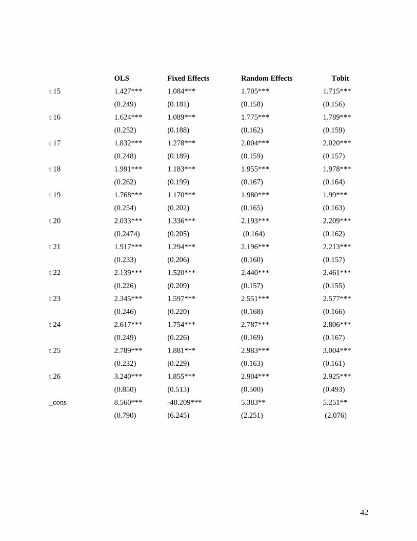
42

OLS Fixed Effects Random Effects Tobit

t 15 1.427***

(0.249)

1.084***

(0.181)

1.705***

(0.158)

1.715***

(0.156)

t 16 1.624***

(0.252)

1.089***

(0.188)

1.775***

(0.162)

1.789***

(0.159)

t 17 1.832***

(0.248)

1.278***

(0.189)

2.004***

(0.159)

2.020***

(0.157)

t 18 1.991***

(0.262)

1.183***

(0.199)

1.955***

(0.167)

1.978***

(0.164)

t 19 1.768***

(0.254)

1.170***

(0.202)

1.980***

(0.165)

1.99***

(0.163)

t 20 2.033***

(0.2474)

1.336***

(0.205)

2.193***

(0.164)

2.209***

(0.162)

t 21 1.917***

(0.233)

1.294***

(0.206)

2.196***

(0.160)

2.213***

(0.157)

t 22 2.139***

(0.226)

1.520***

(0.209)

2.440***

(0.157)

2.461***

(0.155)

t 23 2.345***

(0.246)

1.597***

(0.220)

2.551***

(0.168)

2.577***

(0.166)

t 24 2.617***

(0.249)

1.754***

(0.226)

2.787***

(0.169)

2.806***

(0.167)

t 25 2.789***

(0.232)

1.881***

(0.229)

2.983***

(0.163)

3.004***

(0.161)

t 26 3.240***

(0.850)

1.855***

(0.513)

2.904***

(0.500)

2.925***

(0.493)

_cons 8.560***

(0.790)

-48.209***

(6.245)

5.383**

(2.251)

5.251**

(2.076)

43

OLS Results R Squared 0.712 Adjusted R Squared 0.704 Root MSE 1.439 Prob > F 0.000 No. of Observations 1579

Fixed-effects (within) regression

R Square Within 0.708 R Square Between 0.396 R Square Overall 0.438 Prob >F 0.000 No. of Observations 1579

Random effects GLS regression R Square Within 0.697 R Square Between 0.573 R Square Overall 0.684 Prob >Chi2 0.000 No. of Observations 1579

Random-effects tobit regression Log Likelihood -2093.621 Prob >Chi2 0.000 No. of Observations 1579

44

Table 1B: Import Flows OLS Fixed Effects Random Effects Tobit

exchangerate -0.052***

(0.014)

0.036**

(0.018)

0.046***

(0.017)

0.100***

(0.036)

LangDummy 0.382***

(0.102)

0.535

(0.400)

0.806

(0.539)

LnGDP 0.773***

(0.033)

0.545***

(0.134)

0.728***

(0.093)

0.424**

(0.201)

Lnpop 0.331***

(0.039)

1.180***

(0.307)

0.444***

(0.123)

0.727***

(0.210)

Lndist -0.713***

(0.087)

-0.914***

(0.298)

-0.808*

(0.436)

safta_x -0.631

(0.472)

-0.652*

(0.343)

-0.609*

(0.339)

11.112

(580.128)

bimstec_x 1.743***

(0.527)

1.331***

(0.372)

1.278***

(0.371)

-0.219

(2384.095)

bangkok_x -0.794***

(0.295)

-0.960

(1.187)

13.769

(131.124)

Gcc_x 3.014***

(0.305)

-0.163

(0.451)

0.376

(0.425)

12.686

(126.819)

asean_x -0.005

(0.286)

-0.474**

(0.236)

-0.473**

(0.232)

0.203

(1.255)

Sacu_x -1.882***

(0.400)

-1.512

(1.416)

-2.432*

(1.307)

mercosur_x -0.885***

(0.254)

0.803**

(0.388)

0.749**

(0.379)

13.717

(699.445)

eu_x 1.001***

(0.154)

-0.193

(1.146)

0.679

(0.496)

2.298

(1.477)

Efta_x 0.187

(0.329)

0.411

(1.411)

-0.309

(2.290)

nafta_x 0.632

(0.511)

-0.613*

(0.356)

-0.612*

(0.354)

9.947

(2522.485)

45

Table 1B (continued) OLS Fixed Effects Random Effects Tobit

cis_x -0.762***

(0.267)

0.582**

(0.250)

0.520**

(0.233)

-0.443

(0.903)

t 2 -0.005

(0.333)

0.184

(0.194)

0.180

(0.195)

0.676

(0.591)

t 3 -0.252

(0.333)

-0.096

(0.195)

-0.100

(0.195)

0.520

(0.588)

t 4 -0.079

(0.332)

0.204

(0.196)

0.191

(0.195)

0.984

(0.618)

t 5 0.083

(0.332)

0.378*

(0.196)

0.376*

(0.195)

1.339**

(0.634)

t 6 0.044

(0.331)

0.349*

(0.197)

0.356*

(0.195)

0.965

(0.608)

t 7 -0.119

(0.332)

0.174

(0.198)

0.188

(0.195)

0.843

(0.611)

t 8 -0.102

(0.330)

0.210

(0.196)

0.229

(0.195)

0.723

(0.611)

t 9 0.142

(0.329)

0.3445*

(0.200)

0.373*

(0.195)

1.524**

(0.662)

t 10 0.0283

(0.324)

0.400**

(0.199)

0.433**

(0.192)

0.609

(0.601)

t 11 -0.132

(0.323)

0.206

(0.200)

0.251

(0.192)

0.569

(0.596)

t 12 0.019

(0.323)

0.437**

(0.201)

0.492*

(0.192)

0.313

(0.603)

t 13 0.279

(0.321)

0.707***

(0.202)

0.768***

(0.192)

0.833

(0.627)

t 14 0.370

(0.322)

0.740***

(0.207)

0.815***

(0.197)

0.973

(0.642)

t 15 0.515

(0.319)

0.942***

(0.208)

1.019***

(0.193)

0.844

(0.642)

46

Table 1B (continued) OLS Fixed Effects Random Effects Tobit

t 17 0.674**

(0.321)

1.037***

(0.214)

1.1207***

(0.195)

2.327***

(0.785)

t 18 0.630**

(0.321)

0.984***

(0.217)

1.073***

(0.196)

2.461***

(0.802)

t 19 0.906***

(0.324)

1.280***

(0.222)

1.371***

(0.198)

3.022***

(0.882)

t 20 0.801**

(0.325)

1.174***

(0.225)

1.267***

(0.199)

3.195***

(0.908)

t 21 0.896***

(0.324)

1.292***

(0.227)

1.390***

(0.200)

1.965***

(0.747)

t 22 0.701**

(0.319)

1.194***

(0.228)

1.287***

(0.198)

1.193*

(0.688)

t 23 1.024***

(0.320)

1.454***

(0.232)

1.558***

(0.199)

2.298***

(0.795)

t 24 1.205***

(0.322)

1.615***

(0.236)

1.719***

(0.201)

2.335***

(0.815)

t 25 1.532***

(0.322)

1.937***

(0.241)

2.033***

(0.202)

2.624***

(0.879)

t 26 1.722***

(0.324)

2.101***

(0.242)

2.242***

(0.202)

1.512**

(0.736)

_cons -2.266**

(0.935)

-16.447***

(5.134)

-1.759

(3.267)

0.484

(4.705)

OLS Results

R Squared 0.477 Adjusted R Squared 0.472 Root MSE 2.798 Prob > F 0.000 No. of Observations 3800

Fixed-effects (within) regression

R Square Within 0.254 R Square Between 0.419 R Square Overall 0.353 Prob >F 0.000 No. of Observations 3800

47

Random effects GLS regression R Square Within 0.253 R Square Between 0.526 R Square Overall 0.452 Prob >Chi2 0.000 No. of Observations 3800

Random-effects tobit regression

Log Likelihood -1205.549 Prob >Chi2 0.000 No. of Observations 4175

48

Table 1C: Total Trade (Export and Import) Flows OLS Fixed Effect Random Effect Tobit exchangerate -0.035

(.034)

0.055

(0.047)

0.119***

(.043)

0.105***

(.074)

langdummy 0.305

(.200)

.540

(.166)

1.453*

(.762)

extplnmfn 0.270*

(.149)

0.599***

(0.163)

.534***

(0.152)

1.415***

(0.255)

lngdp 1.906***

(.072)

2.358***

(0.360)

1.816***

(.166)

1.779***

(.200)

lnpop 0.209***

(.080)

6.471***

(0.714)

.459**

(.196)

.870***

(.197)

lndist -2.361***

(.162

-1.846***

(.436)

-2.271***

(.540)

safta_m -1.774**

(.754)

bimstec_m 2.433***

(.887)

bangkok_m -1.446***

(.469)

gcc_m 1.355

(.978)

asean_m 4.635*

(2.547)

.876

(1.322)

.733

(1.355)

-1.013

(2.583)

sacu_m -1.763826

(1.206241)

mercosur_m 0.300

(.661)

1.769

(1.863)

1.697

(2.661)

eu_m 2.307***

(.447)

0.586

(1.309)

1.662**

(.725)

-8.811***

(1.142)

efta_m -0.918

(.809)

2.714

(3.099)

nafta_m -9.027***

(1.798)

-1.135

(1.260)

-2.087

(1.268)

-8.487***

(1.953)

cis_m -0.634

(.737)

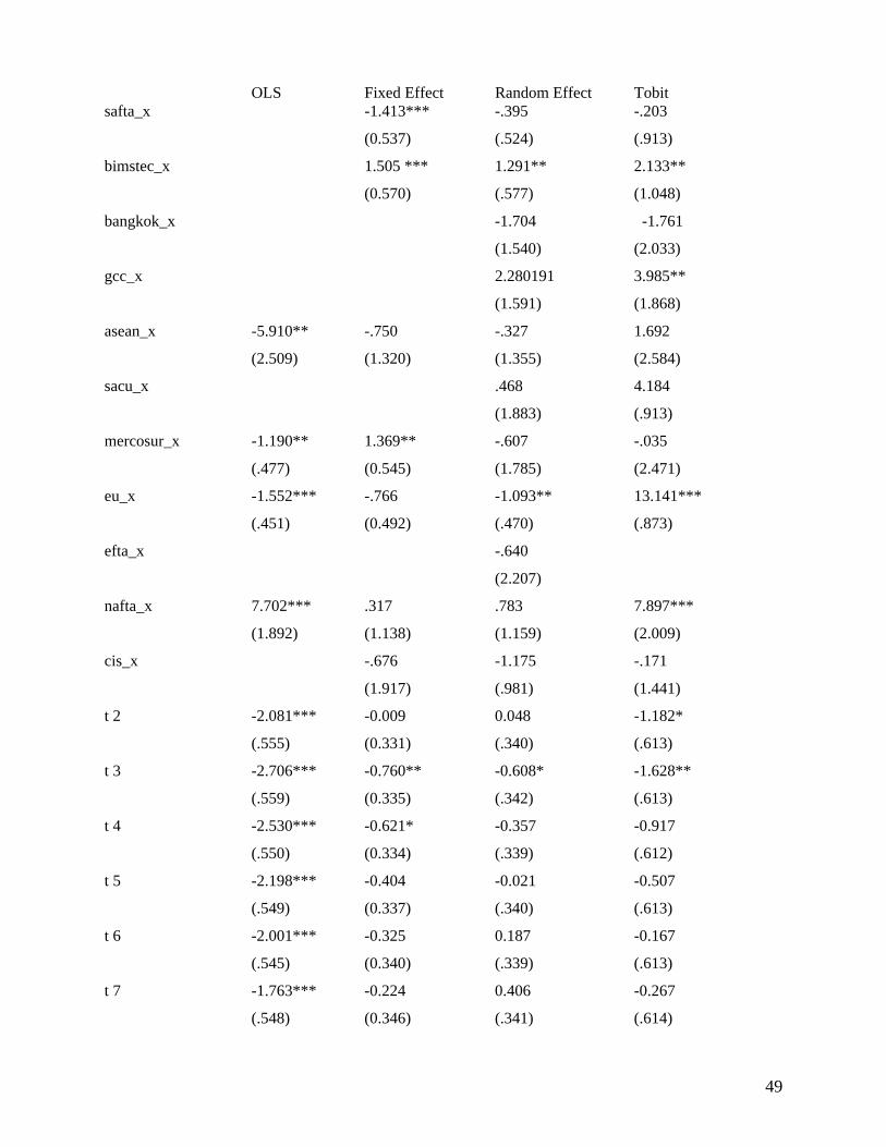
49

OLS Fixed Effect Random Effect Tobit safta_x -1.413***

(0.537)

-.395

(.524)

-.203

(.913)

bimstec_x 1.505 ***

(0.570)

1.291**

(.577)

2.133**

(1.048)

bangkok_x -1.704

(1.540)

-1.761

(2.033)

gcc_x 2.280191

(1.591)

3.985**

(1.868)

asean_x -5.910**

(2.509)

-.750

(1.320)

-.327

(1.355)

1.692

(2.584)

sacu_x .468

(1.883)

4.184

(.913)

mercosur_x -1.190**

(.477)

1.369**

(0.545)

-.607

(1.785)

-.035

(2.471)

eu_x -1.552***

(.451)

-.766

(0.492)

-1.093**

(.470)

13.141***

(.873)

efta_x -.640

(2.207)

nafta_x 7.702***

(1.892)

.317

(1.138)

.783

(1.159)

7.897***

(2.009)

cis_x -.676

(1.917)

-1.175

(.981)

-.171

(1.441)

t 2 -2.081***

(.555)

-0.009

(0.331)

0.048

(.340)

-1.182*

(.613)

t 3 -2.706***

(.559)

-0.760**

(0.335)

-0.608*

(.342)

-1.628**

(.613)

t 4 -2.530***

(.550)

-0.621*

(0.334)

-0.357

(.339)

-0.917

(.612)

t 5 -2.198***

(.549)

-0.404

(0.337)

-0.021

(.340)

-0.507

(.613)

t 6 -2.001***

(.545)

-0.325

(0.340)

0.187

(.339)

-0.167

(.613)

t 7 -1.763***

(.548)

-0.224

(0.346)

0.406

(.341)

-0.267

(.614)

50

t 8 -1.700***

(.537)

-0.260

(0.350)

0.478

(.339)

2.230***

(.617)

t 9 -1.228**

(.544)

0.003

(0.360)

0.902***

(.344)

0.020

(0.623)

t 10 -1.247**

(.547)

-0.120

( 0.367)

0.888***

(.344)

2.492***

(0.625)

t 11 -0.982*

(.550)

0.173

(0.378)

1.308***

(.348)

3.182***

(0.632)

t 12 -0.439

(.550)

0.467

(0.383)

1.664***

(.350)

3.762***

(.640)

t 13 -0.241

(.534)

0.240

(0.383)

1.483***

(.348)

3.439***

(.633)

t 14 -0.286

(.590)

0.623

(0.411)

1.929***

(.374)

3.957***

(.679)

t 15 0.240

(.525)

1.023**

(0.405)

2.459***

(.351)

4.688***

(.638)

t 16 0.612

(.537)

0.925**

(0.423)

2.545***

(.360)

4.561***

(0.656)

t 17 0.711

(.523)

1.028**

( 0.425)

2.696***

(.354)

4.989***

(0.641)

t 18 0.966

(.558)

0.932**

(0.445)

2.696***

(.370)

4.841***

(0.672)

t 19 0.665

(.538)

1.148**

(0.453)

3.003***

(.367)

4.963***

(0.661)

t 20 0.961*

(.517)

1.102**

(0.463)

3.097***

(.365)

5.183***

(.660)

t 21 1.068**

(.485)

1.265***

(0.466)

3.327***

(.356)

5.180***

0.632)

t 22 1.239***

(.452)

1.453***

(0.469)

3.587***

(.347)

5.986***

(0.619)

t 23

1.785***

(0.496)

3.987***

(.373)

6.030***

(.669)

t 24 2.319***

(.513)

2.113***

(0.510)

4.493***

(.375)

6.750***

(.674)

51

t 25 2.738***

(.469)

2.369***

(0.518)

4.883***

(.361)

7.431***

(.643)

t 26 3.107787

(2.040964)

1.532

(1.152)

4.003***

(1.129)

5.745***

(2.141)

_cons 4.011**

(1.751)

-130.6***

(14.026)

-5.646

(4.594)

-13.482**

(6.27)

OLS Results

R Squared 0.674 Adjusted R Squared 0.665 Root MSE 3.482 Prob > F 0.000 No. of Observations 1634

Fixed-effects (within) regression

R Square Within 0.587 R Square Between 0.429 R Square Overall 0.411 Prob >F 0.000 No. of Observations 1634

Random effects GLS regression

R Square Within 0.565 R Square Between 0.654 R Square Overall 0.657 Prob >Chi2 0.000 No. of Observations 1634

Random-effects tobit regression

Log Likelihood -4852.159 Prob >Chi2 0.000 No. of Observations 1758

52

Table 2A: Labour Intensive Activities, Export sequence 2000-06

Sequence Count % of Firms 0 0 0 0 0 0 0 577 30.15 0 0 0 0 0 0 1 16 0.84 0 0 0 0 0 1 0 9 0.47 0 0 0 0 0 1 1 20 1.04 0 0 0 0 1 0 0 6 0.31 0 0 0 0 1 0 1 3 0.16 0 0 0 0 1 1 0 4 0.21 0 0 0 0 1 1 1 12 0.63 0 0 0 1 0 0 0 1 0.05 0 0 0 1 0 1 0 1 0.05 0 0 0 1 1 0 0 4 0.21 0 0 0 1 1 0 1 3 0.16 0 0 0 1 1 1 0 5 0.26 0 0 0 1 1 1 1 13 0.68 0 0 1 0 0 0 0 7 0.37 0 0 1 0 0 0 1 2 0.10 0 0 1 0 0 1 0 1 0.05 0 0 1 0 0 1 1 1 0.05 0 0 1 0 1 0 0 1 0.05 0 0 1 0 1 0 1 2 0.10 0 0 1 0 1 1 1 1 0.05 0 0 1 1 0 0 0 8 0.42 0 0 1 1 0 0 1 1 0.05 0 0 1 1 0 1 0 1 0.05 0 0 1 1 0 1 1 4 0.21 0 0 1 1 1 0 0 1 0.05 0 0 1 1 1 0 1 2 0.10 0 0 1 1 1 1 0 1 0.05 0 0 1 1 1 1 1 12 0.63 0 1 0 0 0 0 0 14 0.73 0 1 0 0 0 1 0 1 0.05 0 1 0 0 1 0 0 2 0.10 0 1 0 0 1 1 0 1 0.05 0 1 0 0 1 1 1 2 0.10 0 1 0 1 0 0 0 2 0.10 0 1 0 1 0 1 1 1 0.05 0 1 0 1 1 0 0 4 0.21 0 1 0 1 1 0 1 1 0.05 0 1 0 1 1 1 0 4 0.21 0 1 0 1 1 1 1 4 0.21 0 1 1 0 0 0 0 4 0.21 0 1 1 0 0 0 1 2 0.10 0 1 1 0 0 1 0 2 0.10 0 1 1 0 0 1 1 1 0.05 0 1 1 0 1 0 0 1 0.05 0 1 1 0 1 1 0 1 0.05 0 1 1 0 1 1 1 2 0.10 0 1 1 1 0 0 0 1 0.05 0 1 1 1 0 0 1 1 0.05 0 1 1 1 0 1 1 2 0.10

53

0 1 1 1 1 0 0 3 0.16 0 1 1 1 1 0 1 2 0.10 0 1 1 1 1 1 0 4 0.21 0 1 1 1 1 1 1 49 2.56 1 0 0 0 0 0 0 64 3.34 1 0 0 0 0 0 1 1 0.05 1 0 0 0 0 1 0 1 0.05 1 0 0 0 0 1 1 3 0.16 1 0 0 0 1 0 0 4 0.21 1 0 0 0 1 0 1 2 0.10 1 0 0 0 1 1 0 1 0.05 1 0 0 0 1 1 1 4 0.21 1 0 0 1 0 0 0 4 0.21 1 0 0 1 0 1 0 1 0.05 1 0 0 1 0 1 1 2 0.10 1 0 0 1 1 0 0 2 0.10 1 0 0 1 1 1 1 7 0.37 1 0 1 0 0 0 0 5 0.26 1 0 1 0 0 1 1 1 0.05 1 0 1 1 0 0 0 2 0.10 1 0 1 1 0 1 1 2 0.10 1 0 1 1 1 0 0 2 0.10 1 0 1 1 1 0 1 1 0.05 1 0 1 1 1 1 0 5 0.26 1 0 1 1 1 1 1 19 0.99 1 1 0 0 0 0 0 42 2.19 1 1 0 0 0 0 1 4 0.21 1 1 0 0 0 1 1 4 0.21 1 1 0 0 1 0 0 2 0.10 1 1 0 0 1 0 1 1 0.05 1 1 0 0 1 1 1 3 0.16 1 1 0 1 0 0 0 4 0.21 1 1 0 1 0 1 1 1 0.05 1 1 0 1 1 0 1 1 0.05 1 1 0 1 1 1 0 8 0.42 1 1 0 1 1 1 1 26 1.36 1 1 1 0 0 0 0 37 1.93 1 1 1 0 0 0 1 2 0.10 1 1 1 0 0 1 0 1 0.05 1 1 1 0 0 1 1 5 0.26 1 1 1 0 1 0 0 3 0.16 1 1 1 0 1 0 1 1 0.05 1 1 1 0 1 1 0 3 0.16 1 1 1 0 1 1 1 22 1.15 1 1 1 1 0 0 0 26 1.36 1 1 1 1 0 0 1 3 0.16 1 1 1 1 0 1 0 2 0.10 1 1 1 1 0 1 1 19 0.99 1 1 1 1 1 0 0 31 1.62 1 1 1 1 1 0 1 11 0.57 1 1 1 1 1 1 0 56 2.93 1 1 1 1 1 1 1 633 33.07 Total 1914

54

Table 2B: Manufacturing Activities: Export sequence from 2000-06

Sequence Count % of Firms 1111111 716 21.130000000 1398 41.260000001 75 2.210000010 30 0.880000011 55 1.620000100 22 0.650000101 13 0.380000110 18 0.530000111 47 1.390001000 13 0.380001001 2 0.060001010 2 0.060001011 6 0.180001100 11 0.320001101 6 0.180001110 25 0.740001111 60 1.770010000 15 0.440010001 6 0.180010010 1 0.030010011 2 0.060010100 4 0.120010101 2 0.060010111 5 0.150011000 17 0.500011001 3 0.090011010 2 0.060011011 6 0.180011100 4 0.120011101 4 0.120011110 7 0.210001110 25 0.741001000 5 0.150100001 1 0.031011111 27 0.800100010 1 0.030100111 4 0.120110010 1 0.030110011 2 0.060111110 21 0.621011000 5 0.150101100 6 0.180111000 10 0.301010010 1 0.030101001 2 0.060110110 2 0.061010101 1 0.031001001 1 0.030111111 71 2.101011011 5 0.15

55

0111100 13 0.381000100 3 0.091010111 2 0.060100110 3 0.091100011 4 0.120101101 2 0.061011101 1 0.030101000 1 0.030101111 10 0.301001011 2 0.060111101 7 0.210111011 2 0.060110000 11 0.321010000 13 0.380111001 4 0.121000000 95 2.801000011 1 0.030100100 4 0.120101011 2 0.061000110 2 0.061101110 6 0.181101100 4 0.121111110 64 1.891111101 19 0.561111100 34 1.001111011 25 0.741111010 5 0.151111001 4 0.121111000 37 1.091110101 4 0.121001110 3 0.091100110 2 0.060110111 5 0.150100000 27 0.800000010 30 0.890011111 44 1.300101010 1 0.030101110 4 0.120110001 2 0.060110100 2 0.061000001 2 0.061000111 7 0.211001010 2 0.061001100 1 0.031001111 12 0.351011010 1 0.031011100 4 0.121011110 5 0.151100000 54 1.601100001 6 0.181100100 5 0.151100101 2 0.061100111 7 0.21

56

1101000 8 0.24Total Plants 3388

57

Table 3: Labour Intensive Activities: The Decision to Export

Table 3A: Probit Model

Explanatory Variable

Model I Model II Model II Model IV

Lagex 0.02***(0.00) 0.03*** (0.00)

Scale it-1 0.00*** (0.00)

Energy it-1 -0.00 (0.00)

Wage it-1 -0.01*** (0.00) -0.01*** (0.00) -0.01*** (0.00) -0.01*** (0.00)

LP it-1 0.18** (0.07)

RD it-1 0.55*** (0.08) 0.57*** (0.08)

SelCost it-1 -0.07 (0.01) 0.14** (0.00) -0.08 (0.01) -0.12 (0.00)

Profit it-1 0.00** (0.00) 0.00*** (0.00) 0.00** (0.00) 0.00*** (0.00)

NFA it-1 -0.00** (0.00) -0.00 (0.00) -0.00** (0.00) -0.00** (0.00)

Wshare1 it-1 0.00*** (0.00)

IMP it-1 0.01*** (0.00) 0.00*** (0.00)

Intercept 0.24*** (0.02) 0.54*** (0.02) 0.25*** (0.02) 0.30*** (0.02)

R2 0.16 0.05 0.15 0.09

Note: standard error in parenthesis; * significant at 10 percent, ** significant at 5 percent, *** significant at 1 percent Dependent variable Y = 1 for exporting years = 0 for non-exporting years

58

Table 3B: Logit Model

Note: standard error in parenthesis; * significant at 10 percent, ** significant at 5 percent, *** significant at 1 percent Dependent variable Y = 1 for exporting years = 0 for non-exporting years

Explanatory Variable

Model I Model II Model II Model IV

Lagex 0.09***(0.00) 0.08***(0.01)

Scale it-1 0.01***(0.00)

Energy it-1 -0.00**(0.00)

Wage it-1 -0.01***(0.00) -0.02***(0.00) -0.02***(0.00) -0.02***(0.00)

LP it-1 0.39**(0.15)

RD it-1 1.07***(0.19) 1.30***(0.19)

SelCost it-1 -0.00(0.00) -0.00(0.00) 0.00**(0.00) -0.00(0.00)

Profit it-1 0.00**(0.00) 0.00*(0.00) 0.00***(0.00) 0.00**(0.00)

NFA it-1 -0.00*(0.00) -0.00**(0.00) -0.00(0.00) -0.00*(0.00)

WS it-1 0.00***(0.00)

IMP it-1 0.00***(0.00) 0.00***(0.00) 0.01***(0.00) 0.00***(0.00)

Intercept 0.24**(0.04) 0.35***(0.04) 0.20***(0.04) 0.21***(0.05)

R2 0.16 0.11 0.06 0.19

59

Table 3C: Tobit Model

Explanatory variables

Model I Model II Model III Model IV

Lag EX 0.19***(0.01) 0.19***(0.00)

Energyit-1 -0.00(0.00)

Wage it-1 -0.73***(0.06) -0.86***(0.06) -0.94***(0.06) -0.71**(0.06)

RD it-1 0.24(0.61) 0.11(0.59)

SelCost it-1 0.00(0.00) 0.00(0.00) 0.00(0.00) -0.00(0.00)

Profit it-1 0.00***(0.00) 0.00(0.00) 0.00***(0.00) 1.68(2.09)

LP it-1 0.44(0.39)

IMP it-1 0.00**(0.00) 0.01***(0.00)

Size it-1 0.03***(0.00)

Wshare it-1 0.01**(0.00)

NFA it-1 -0.00(0.00) -0.00*(0.00) -0.00(0.00) -0.00**(0.00)

Constant 14.05***(0.78) 15.88***(0.87) 19.05***(0.79) 14.79***(0.82)

R2 0.02 0.01 0.01 0.02

Note: standard error in parenthesis Dependent variable = 0 for the non-exporting years and export as percentage of total sales if they did export in period t.

60

Table 3D: Linear Probability Model

Explanatory Variable Fixed Effects

No. of employee -0.00 (0.00)

NFA/employ -4.433( 1.526)***

Wage -0.00 (0.00)

R&D 4.48 (1.24)***

LP 25.012( 4.41) ***

Selcost 2.488( 0.169)***

Profit 0.04( 0.05)

Intercept 14.306( 1.24) ***

61

Table 4: Manufacturing Sector

Table 4A: CMIE Data, Logit And Probit Models (Panel)

Explanatory variables

Logit Probit

Scaleit-1 0.00***(0.00) 0.01*** (0.00)

Energyit-1 -0.03***(0.00) -0.02*** (0.00)

Wageit-1 -0.01***(0.00) -0.01*** (0.00)

R&Dit-1 0.01***(0.00) 0.01*** (0.00)

PBTit-1 -0.00(0.00) -0.00 (0.00)

IMPit-1 0.02***(0.00) 0.01*** (0.00)

Wshareit-1 -0.00(0.00) 0.00*(0.00)

Sellcostit-1 0.001(0.00) 0.01** (0.00)

NFAit-1 -0.001***(.000) -0.00*** (0.00)

_cons 0.34***(0.03) 0.36*** (0.01)

R2 0.13 0.09

No. of obs. 17167 17167

Note: Std Error in the parentheses * Significant at 10 percent, ** significant at 5 percent, *** significant at 1 percent Dependent variable Y = 1 for exporting years; = 0 for non-exporting years

62

Table 4B: CMIE Data, Tobit Model (Panel) Explanatory variables Model I Model II

LagEx 0.02***(0.00)

Scaleit-1 0.00 (0.00)

Energyit-1 -0.01***(0.00) -0.01*** (0.00)

Wageit-1 -0.01***(0.00) -0.00*** (0.00)

R&Dit-1 0.01(0.00) 0.01 (0.00)

PBTit-1 -0.00(0.00) -0.00 (0.00)

IMPit-1 0.02***(0.00) 0.01*** (0.00)

Wshareit-1 0.03***(0.00) 0.02***(0.00)

Sellcostit-1 0.001(0.00) -0.01 (0.00)

NFAit-1 -0.001(.000) -0.00 (0.00)

_cons 4.73***(0.05) 4.44*** (0.05)

No. of obs. 17167 17167

Note: Std Error in parentheses * Significant at 10 percent, ** significant at 5 percent, *** significant at 1 percent For Tobit Model: Dependent variable = 0 for the non-exporting years Export as percentage of total sales if they did export in period t.

63

Table 4C: Manufacturing Activities (CII data): Probit and Logit Model

Variables Probit Model Logit Model

Scale 0.57*** (0.20) 0.99*** (0.35)

Own 0.86***(0.19) 1.50*** (0.34)

Sale/no of emp -0.42(0.58) -0.74(0.95)

CP -5.00e-07(1.55e-06) -2.80e-07(9.75e-07)

Const 0.07(0.09) 0.11(0.15)

Note: standard error in parenthesis Dependent variable = 1 for exporting firms and = 0 for non-exporting firms Scale is a dummy that takes value 1 if it is a large firm and 0 otherwise Own is a dummy variable which is equal to 1 if firm either have a JV/Collaboration /foreign parent and 0 otherwise C P (capital productivity) = total turnover/ investment

Table 4D: Manufacturing Activities (CII data), Tobit Model

Note: standard error in parenthesis Dependent variable = 0 for the non-exporting years Export as percentage of total sales if they did export in period t. Scale is a dummy that takes value = 1 if it is a large firm and = 0 otherwise Own is a dummy that takes value = 1 if firm either have a JV/Collaboration /foreign parent and 0 otherwise CP (capital productivity) = total turnover/ investment

Variables Tobit Model

Scale 1.80***(0.94)

Own 2.39***(0.85)

Sale/no of emp -0.23(2.88)

CP -2.30e-07 (4.74e-06)

Const 4.82***(0.48)

64

Table 5: Multinomial Logistic Model of Logodds Table 5A: Model I

Log Odds of Category j Relative to Category 3, j = 1, 2 and 4 Category 3 and 1 Category 3 and 2 Category 3 and 4 Scale 0.007***

(0.002) 0.016*** (0.001)

0.011*** (0.00)

Wage -0.035*** (0.011)

-0.022*** (0.002)

-0.00 (0.00)

R&D 0.893** (0.418)

1.212*** (0.230)

0.253 (0.223)

Sel Cost -0.133*** (0.034)

0.003** (0.001)

0.004*** (0.00)

Profit 0.001(0.00)

0.001*** (0.00)

0.00* (0.00)

NFA -0.00 (0.00)

-0.01*** (0.00)

-0.00 (0.00)

IMP 0.001*** (0.00)

0.001*** (0.00)

-0.001 (0.001)

Const -1.356*** (0.156)

0.673*** (0.059)

-0.491*** (0.063)

Pseudo R2 0.093 0.093 0.093 Here,

η1i = -1.356 + 0.007 *Scalei – 0.035*Wi + 0.893* RDi – 0.133* Selcosti + 0.001* Pi – 0.000*

NFAi + 0.001* Impi

η2i = -0.673 + 0.016 *Scalei – 0.022*Wi + 1.212* RDi + 0.003* Selcosti + 0.001* Pi – 0.000*

NFAi + 0.001* Impi

η4i = -0.491 + 0.011 *Scalei – 0.000*Wi + 0.253* RDi + 0.004* Selcosti + 0.000* Pi – 0.000*

NFAi - 0.001* Impi

The average values of the explanatory variables are:

Variables mean Scale 51.98795 W 21.83567 RD 0.064151 Selcost 13.34933 P -71.0495 NFA 2.212833 Imp 27.13816

65

From the above we get:

η1 = -1.356 + 0.007 *51.98 – 0.035*21.83 + 0.893* 0.064 – 0.133* 13.349 + 0.001* (-71.049) – 0.000*

2.21 + 0.001* 27.13 = -3.47974

η2 = -0.673 + 0.016 *51.98 – 0.022*21.83 + 1.212* 0.064 + 0.003* 13.349 + 0.001* (-71.049) – 0.000*

2.21 + 0.001* 2.21 = 1.189427

η4 = -0.491 + 0.011 *51.98 – 0.000*21.83 + 0.253* 0.064 + 0.004* 13.349 + 0.000* (-71.049) – 0.000*

2.21 - 0.001* 27.13 = 0.0870501

From these we can compute the probabilities as:

Pr (Category = 1) = exp (η1) / 1+ exp (η1) + exp (η2) + exp (η4) = exp (-3.47974) / 1+ exp (-3.47974) +

exp (1.189427) + exp (0.0870501) = 0.005699

Pr (Category =2) = exp (η2) / 1+ exp (η1) + exp (η2) + exp (η4) = exp (1.189427) / 1+ exp (-3.47974) +

exp (1.189427) + exp (0.0870501) = 0.607586

Pr (Category =4) = exp (η4) / 1+ exp (η1) + exp (η2) + exp (η4) = exp ((0.0870501) / 1+ exp (-3.47974) +

exp (1.189427) + exp (0.0870501) = 0.201768

Pr (Category =3) = 1 / 1+ exp (η1) + exp (η2) + exp (η4) = 1 / 1+ exp (-3.47974) + exp (1.189427) + exp

(0.0870501) = 0.184947

66

Table 5B: MODEL II

Log Odds of Category j Relative to Category 3 Category 3 and 1 Category 3 and 2 Category 3 and 4 Wage -0.026***

(0.010) -0.023*** (0.002)

-0.001*** (0.00)

Sel Cost -0.15*** (0.037)

0.007*** (0.002)

0.006*** (0.002)

Profit 0.00 (0.00)

0.001*** (0.00)

0.00 (0.00)

NFA -0.001***(0.00) -0.001*** (0.00)

-0.001*** (0.00)

NVA/W 0.003 (0.00)

0.005*** (0.001)

-0.007** (0.003)

IMP 0.005*** (0.001)

0.005*** (0.001)

-0.006*** (0.003)

Const -1.16*** (0.0147)

1.457*** (0.048)

-0.077 (0.053)

Pseudo R2 0.045 0.045 0.045 No. of obs 5384 5384 5384 Similarly with the same argument as before the probabilities for different categories for model II are as

follows:

Pr (category 1/ Z1, Z2, --------- Zk) = 0.009113533

Pr (category 2/ Z1, Z2, --------- Zk ) = 0.395313519

Pr (category 4/ Z1, Z2, --------- Zk) = 0.263265701

Pr (Category 3/ Z1, Z2, --------- Zk ) = 0.332307247

67

Table 5C: MODEL III

Log Odds of Category j Relative to Category 3 Category 3 and 1 Category 3 and 2 Category 3 and 4 LagEx -0.011

(0.091) 0.501*** (0.036)

0.457*** (0.036)

Wage -0.037*** 0.011

-0.011*** (0.002)

-0.000* (0.00)

NVA/W 0.163 (0.318)

0.222 (0.175)

-0.070 (0.233)

R&D 0.897*** (0.379)

1.166*** (0.235)

0.138 (0.231)

Sel Cost -0.033 (0.026)

0.003** (0.001)

0.003*** (0.001)

Profit 0.00 (0.00)

-0.00* (0.00)

8.86E-05 (0.00)

NFA 0.00 (0.00)

-0.001*** (0.00)

-3.6E-05 (0.00)

IMP 0.002 (0.002)

0.007*** (0.001)

-0.00 (0.001)

Const -1.404*** (0.138)

0.258*** (0.057)

-0.745*** (0.058)

Pseudo R2

Similarly with the same argument as before the probabilities for different categories for model III

are as follows:

Pr (category 1/ Z1, Z2, --------- Zk) = 0.0000544

Pr (category 2/ Z1, Z2, --------- Zk ) = 0.840455725

Pr (category 4/ Z1, Z2, --------- Zk) = 0.158680631

Pr (Category 3/ Z1, Z2, --------- Zk) = 0.000809

68

Table 5D: MODEL IV

Log Odds of Category j Relative to Category 3 Category 3 and 1 Category 3 and 2 Category 3 and 4 LagEx 0.307***

(0.036) 0.507*** (0.034)

0.457*** (0.034)

Energy -0.017*** (0.004)

0.000 (0.003)

0.004 (0.004)

Wage 0.001*** (0.000)

-0.010*** (0.002)

0.000 (0.001)

Sel cost 0.001 (0.001)

0.000 (0.001)

0.002*** (0.001)

Profit 0.001 (0.001)

0.000 (0.000)

0.000*** (0.000)

IMP 0.071*** (0.005)

0.007 (0.005)

0.000 (0.006)

Const -1.436*** (0.076)

0.096 (0.060)

-0.885***(0.065)

Pseudo R2

Similarly as analyzed previously, the probabilities for different categories are:

Pr (category 1) = 0.08253465

Pr (category 2) = 0.75683073

Pr (category 4) = 0.159717171

Pr (Category 3) = 0.000917444

69

Appendix: Table A: List of RTAs Covered

SACU GCC BIMSTEC Bangkok EFTA

South Africa Bahrain Bangladesh Bangladesh Norway Lesotho Kuwait Bhutan Laos Switzerland Swaziland Oman Nepal Republic of Korea Iceland Botswana Qatar Sri Lanka Sri Lanka Liechtenstein Namibia UAE Thailand Philippines Myanmar Thailand India India ASEAN SAFTA MERCOSUR CIS NAFTA EU Indonesia India Spain Azerbaijan Canada Austria Malaysia Bangladesh Portugal Armenia USA Belgium Philippines Bhutan Brazil Belarus Mexico Bulgaria Singapore Nepal Argentina Georgia Cyprus Thailand Sri Lanka Uruguay Kazakhstan Czech Republic Brunei Pakistan Paraguay Kyrgyz Denmark Vietnam Maldives Bolivia Moldova Estonia Lao PDR Chile Russia Finland Myanmar Columbia Tajikistan France Cambodia Ecuador Uzbekistan Germany Peru Ukraine Greece

Hungary Ireland Italy Latvia Lithuania Luxembourg Malta Netherlands Poland Portugal Romania Slovakia Slovenia Spain Sweden United Kingdom

70

Appendix: Table B: Export of Principal Commodities (in US $) from India (April-February, 2005-06 and 2006-07) (US $ Million)

Commodities 2005-06 April-Feb

2006-07 April-Feb

% Growth % Share

I. Plantation 673.75 787.85 16.94 0.7 1. Tea 359.25 409.61 14.02 0.36 2. Coffee 314.5 378.24 20.27 0.34 II. Agri & Allied Products 6365.16 7492.72 17.71 6.66 III. Marine Products 1446.44 1413.53 -2.28 1.26 IV. Ores & Minerals 5283.2 5959.08 12.79 5.3 V. Leather & Mfrs. 2434.8 2657.68 9.15 2.36 1. Footwear 947.27 1124.53 18.71 1 2. Leather & mfrs. 1487.54 1533.15 3.07 1.36 VI. Gems & Jewellery 13867.33 13785 -0.59 12.26 VII. Sports Goods 120.35 116.56 -3.15 0.1 VIII. Chemicals & Related Products 13823.27 15787.94 14.21 14.04 1. Basic chemls., Pharma & cosmetics 7971.03 9223 15.71 8.2 2. Plastics & Linoleum 2539.82 2892.45 13.88 2.57 3. Rubber, glass & other products 2664.88 3008.09 12.88 2.68 4. Residual chemls. & allied products 647.54 664.39 2.6 0.59 IX. Engineering Goods 16860.21 23171.06 37.43 20.61 A. Machinery 8375.28 10251.05 22.4 9.12 1. Machine tools 207.02 212.47 2.64 0.19 2. Machinery & Instruments 4468.17 5839.53 30.69 5.19 3. Transport equipments 3700.09 4199.04 13.48 3.73 B. Iron and Steel 3134.38 4680.62 49.33 4.16 C. Other Engineering items 5350.54 8239.39 53.99 7.33 1. Ferro Alloys 227.81 312.19 37.04 0.28 2. Aluminium other than prods. 180.52 262.37 45.34 0.23 3. Non-ferrous metals 1112.46 3154.76 183.58 2.81 4. Manufacture of metals 3767.87 4439.47 17.82 3.95 5. Residual Engineering Items 61.89 70.61 14.09 0.06 X. Electronic Goods 1994.56 2569.2 28.81 2.29 1. Electronics 1910.51 2522.76 32.05 2.24 2. Computer Software in physical form 84.06 46.44 -44.75 0.04 XI. Project Goods 134.84 90.88 -32.6 0.08 XII. Textiles 13836.19 14467.43 4.56 12.87 1. Readymade garments 7626.46 7844.17 2.85 6.98 2. Cotton, yarn, fabrics, made-ups, etc. 3533.86 3674.37 3.98 3.27 3. Manmade textiles made-ups, etc. 1813.95 2104.62 16.02 1.87 4. Natural silk textiles 394.29 396.32 0.51 0.35 5. Wool & woollen mfrs. 77.15 75.36 -2.33 0.07 6. Coir & coir mfrs. 122.28 129.26 5.71 0.11 7. Jute mfrs. 268.18 243.34 -9.26 0.22 XIII. Handicrafts 421.93 339 -19.65 0.3 XIV. Carpets 762.5 812.92 6.61 0.72 XV. Cotton Raw Incl. Waste 504.63 1107.29 119.43 0.98 XVI. Petroleum Products 10624.02 16889.83 58.98 15.02 XVII. Unclassified Exports 2299.34 4989.7 117.01 4.44 Grand Total 91452.54 112437.68 22.95 100 Source: Ministry of Commerce & Industry, Govt. of India Note: US Dollar Exchange Rate of April-February 2005-06 is 44.2546 and April-February 2006-07 is 45.4019

71

Appendix Table C: