indirect identification of horizontal gene transfer
TRANSCRIPT

Journal of Mathematical Biology (2021) 83:10https://doi.org/10.1007/s00285-021-01631-0 Mathematical Biology
Indirect identification of horizontal gene transfer
David Schaller1,2,3 ·Manuel Lafond4 · Peter F. Stadler2,3,6,7,8,9,10,11,12 ·Nicolas Wieseke5 ·Marc Hellmuth13
Received: 16 December 2020 / Revised: 6 April 2021 / Accepted: 13 June 2021/ Published online: 3 July 2021© The Author(s) 2021
AbstractSeveral implicit methods to infer horizontal gene transfer (HGT) focus on pairs ofgenes that have diverged only after the divergence of the two species in which thegenes reside. This situation defines the edge set of a graph, the later-divergence-time (LDT) graph, whose vertices correspond to genes colored by their species. Weinvestigate these graphs in the setting of relaxed scenarios, i.e., evolutionary scenariosthat encompass all commonly used variants of duplication-transfer-loss scenarios inthe literature. We characterize LDT graphs as a subclass of properly vertex-coloredcographs, and provide a polynomial-time recognition algorithm aswell as an algorithmto construct a relaxed scenario that explains a given LDT. An edge in an LDT graphimplies that the two corresponding genes are separated by at least one HGT event. Theconverse is not true, however.We show that the complete xenology relation is describedby an rs-Fitch graph, i.e., a complete multipartite graph satisfying constraints on thevertex coloring. This class of vertex-colored graphs is also recognizable in polynomialtime. We finally address the question “how much information about all HGT eventsis contained in LDT graphs” with the help of simulations of evolutionary scenarioswith a wide range of duplication, loss, and HGT events. In particular, we show that asimple greedy graph editing scheme can be used to efficiently detect HGT events thatare implicitly contained in LDT graphs.
Keywords Gene families · Xenology · Binary relation · Indirect phylogeneticmethods · Horizontal gene transfer · Fitch graph · Later-divergence-time ·Polynomial-time recognition algorithm
Mathematics Subject Classification 92-08 · 92D15 · 68R01
B Marc [email protected]
Extended author information available on the last page of the article
123

10 Page 2 of 73 D. Schaller et al.
1 Introduction
Horizontal gene transfer (HGT) laterally introduces foreign genetic material into agenome. The phenomenon is particularly frequent in prokaryotes (Soucy et al. 2015;Nelson-Sathi et al. 2015) but also contributed to shaping eukaryotic genomes (Keelingand Palmer 2008; Husnik and McCutcheon 2018; Acuña et al. 2012; Li et al. 2014;Moran and Jarvik 2010; Schönknecht et al. 2013). HGT may be additive, in whichcase its effect is similar to gene duplications, or lead to the replacement of a verticallyinherited homolog. From a phylogenetic perspective, HGT leads to an incongruenceof gene trees and species trees, thus complicating the analysis of gene family histories.
A broad spectrum of computational methods have been developed to identify hor-izontally transferred genes and/or HGT events, recently reviewed by Ravenhall et al.(2015). Parametricmethods use genomic signatures, i.e., sequence features specific to a(group of) species identify horizontally inserted material. Genomic signatures includee.g. GC content, k-mer distributions, sequence autocorrelation, or DNA deformability(Dufraigne et al. 2005; Becq et al. 2010). Direct (or “explicit”) phylogenetic methodsstart from a given gene tree T and species tree S and compute a reconciliation, i.e., amapping of the gene tree into the species tree. This problem first arose in the contextof host/parasite assemblages (Page 1994; Charleston 1998) considering the equivalentproblem of mapping a parasite tree T to a host phylogeny S such that the number ofevents such as host-switches, i.e., horizontal transfers, is minimized. For a review ofthe early literature we refer to Charleston and Perkins (2006). A major difficulty is toenforce time consistency in the presence of multiple horizontal transfer events, whichrenders the problem of finding optimal reconciliations NP-hard (Hallett and Lagergren2001; Ovadia et al. 2011; Tofigh et al. 2011; Hasic and Tannier 2019). Neverthelessseveral practical approaches have become available, see e.g. Tofigh et al. (2011), Chenet al. (2012) and Ma et al. (2018).
Indirect (or “implicit”) phylogenetic methods forego the reconstruction of trees andstart from sequence similarity or evolutionary distances and use unexpectedly smallor large distances between genes as indicators of HGT. While indirect methods havebeen used successfully in the past, reviewed by Ravenhall et al. (2015), they havereceived very little attention from a more formal point of view. In this contribution,we focus on a particular type of implicit phylogenetic information, following theideas of Novichkov et al. (2004). The basic idea is that the evolutionary distancebetween orthologous genes is approximately proportional to the distances betweentheir species. Xenologous gene pairs as well as duplicate genes thus appear as outliers(Lawrence and Hartl 1992; Clarke et al. 2002; Novichkov et al. 2004; Dessimoz et al.2008). More precisely, consider a family of homologous genes in a set of speciesand plot the phylogenetic distance of pairs of most similar homologs as a function ofthe phylogenetic distances between the species in which they reside. Since distancesbetween orthologous genes can be expected to be approximately proportional to thedistances between the species, orthologous pairs fall onto a regression line that definesequal divergence time for the last common ancestor of corresponding gene and speciespairs. The gene pairs with “later divergence times”, i.e., those that are more closelyrelated than expected from their species, fall below the regression line (Novichkovet al. 2004). Kanhere and Vingron (2009) complemented this idea with a statistical
123

Indirect identification of horizontal gene transfer Page 3 of 73 10
test based on the Cook distance to identify xenologous pairs in a statistically soundmanner. For the mathematical analysis we assume that we can perfectly identify allpairs of genes a and b that aremore closely related than expected from the phylogeneticdistance of their respective genomes. Naturally, this defines a graph (G, σ ), whosevertices x (the genes) are colored by the species σ(x) in which they appear. Here, weare interested in two questions:
(1) What are the mathematical properties that characterize these “later-divergence-time” (LDT ) graphs?
(2) What kind of information about HGT events, the gene and species tree, and thereconciliation map between them is contained implicitly in an LDT graph?
In Sect. 6 we will briefly consider the situation that later-divergence-time informationis fraught with experimental errors.
These questions are motivated by a series of recent publications that characterizedthemathematical structure of orthology (Hellmuth et al. 2013; Lafond andEl-Mabrouk2014), the xenology relation sensu Fitch (Geiß et al. 2018; Hellmuth et al. 2018; Hell-muth and Seemann 2019), and the (reciprocal) best match relation (Geiß et al. 2019,2020b; Schaller et al. 2021a, b). Each of these relations satisfies stringent mathemati-cal conditions that—at least in principle—can be used to correct empirical estimatesand thus serve as a potential means of noise reduction (Hellmuth et al. 2015; Stadleret al. 2020). This approach has also lead to efficient algorithms to extract gene trees,species trees, and reconciliations from the relation data. Although the resulting rep-resentations of gene family histories are usually not fully resolved, they can provideimportant constraints for subsequent refinements. The advantage of the relation-basedapproach is primarily robustness. While the inference of phylogenetic trees relies ondetailed probability models or the additivity of distance metrics, our approach startsfrom yes/no answers to simple, pairwise comparisons. These data can therefore berepresented as edges in a graph, possibly augmented by a measure of confidence.Noise and inaccuracies in the initial estimates then translate into violations of therequired mathematical properties of the graphs in question. Graph editing approachescan therefore be harnessed as a means of noise reduction (Hellmuth et al. 2015; Dondiet al. 2017; Lafond and El-Mabrouk 2014; Lafond et al. 2016; Hellmuth et al. 2020b, a;Schaller et al. 2021c).
Previous work following this paradigm has largely been confined to duplication-loss (DL) scenarios, excluding horizontal transfer. As shown in Hellmuth (2017), it ispossible to partition a gene set into HGT-free classes separated by HGTs. Within eachclass, the reconstruction problems then simplify to the much easier DL scenarios. It isof utmost interest, therefore, to find robust methods to infer this partition directly from(dis)similarity data. Here, we explore the usefulness and limitations of LDT graphsfor this purpose.
This contribution is organized as follows. After introducing the necessary notation,we introduce relaxed scenarios, a very general framework to describe evolutionaryscenarios that emphasizes time consistency of reconciliation rather than particulartypes of evolutionary events. In Sect. 4, LDT graphs are defined formally and char-acterized as those properly colored cographs for which a set of accompanying rootedtriples is consistent (Theorem 3). The proof is constructive and provides a method
123

10 Page 4 of 73 D. Schaller et al.
(Algorithm 1) to compute a relaxed scenario for a given LDT graph. Section 5 definesHGT events, shows that every edge in a LDT graph corresponds to an HGT event,and characterizes those LDT graphs that already capture all HGT events. In addition,we provide a characterization of “rs-Fitch graphs” (general vertex-colored graphs thatcapture all HGT events) in terms of their coloring. These properties can be verified inpolynomial time. Since LDT graphs do not usually capture all HGT events, we dis-cuss in “Appendix C” several ways to obtain a plausible set of HGT candidates fromLDT graphs. In Sect. 7, we address the question “how much information about allHGT events is contained in LDT graphs” with the help of simulations of evolutionaryscenarios with a wide range of duplication, loss, and HGT events. We find that LDTgraphs cover roughly a third of xenologous pairs, while a simple greedy graph editingscheme can more than double the recall at moderate false positive rates. This greedyapproach already yields amedian accuracy of 89%, and in 99.8%of the cases producesbiologically feasible solutions in the sense that the inferred graphs are rs-Fitch graphs.We close with a discussion of several open problems and directions for future researchin Sect. 8.
Thematerial of this contribution is extensive and contains several lengthy, very tech-nical proofs. We therefore divided the presentation into a Narrative Part that containsonly those mathematical results that contribute to our main conclusions, and a Tech-nical Part providing additional results and all proofs. To facilitate cross-referencingbetween the two parts, the same numbering of Definitions, Lemmas, Theorems, etc., isused. Appendices A, B, and C contain the technical material corresponding to Sects. 4,5, and 6, respectively.
2 Notation
Graphs We consider undirected graphs G = (V , E) with vertex set V (G) := V andedge set E(G) := E , and denote edges connecting vertices x, y ∈ V by xy. Thegraphs K1 and K2 denote the complete graphs on one and two vertices, respectively.The graph K2 + K1 is the disjoint union of a K2 and a K1.
The join G � H of two graphs G = (V , E) and H = (W , F) is the graph withvertex set V ∪· W and edge set E ∪· F ∪· {xy | x ∈ V , y ∈ W }. We write H ⊆ G ifV (H) ⊆ V (G) and E(H) ⊆ E(G), in which case H is called a subgraph of G. Givena graph G = (V , E), we write G[W ] for the graph induced by W ⊆ V . A connectedcomponent C of G is an inclusion-maximal vertex set such that G[C] is connected.A (maximal) clique C in an undirected graph G is an (inclusion-maximal) vertex setsuch that, for all vertices x, y ∈ C , it holds that xy ∈ E(G), i.e., G[C] is complete. AsubsetW ⊆ V is a (maximal) independent set if G[W ] is edgeless (andW is maximalw.r.t. inclusion). A graph G = (V , E) is complete multipartite if V consists of k ≥ 1pairwise disjoint independent sets I1, . . . , Ik and xy ∈ E if and only if x ∈ Ii andy ∈ I j with i �= j .
A graphG together with a vertex coloring σ , denoted by (G, σ ), is properly coloredif uv ∈ E(G) implies σ(u) �= σ(v). For a coloring σ : V → M and a subset W ⊆ V ,we write σ(W ) := {σ(w) | w ∈ W } for the set of colors that appear on the vertices inW . Throughout, we will need restrictions of the coloring map σ .
123
Indirect identification of horizontal gene transfer Page 5 of 73 10
Definition 1 Let σ : L → M be a map, L ′ ⊆ L and σ(L ′) ⊆ M ′ ⊆ M . Then, the mapσ|L ′,M ′ : L ′ → M ′ is defined by putting σ|L ′,M ′(v) = σ(v) for all v ∈ L ′. If we onlyrestrict the domain of σ , we just write σ|L ′ instead of σ|L ′,M .
We do neither assume that σ nor that its restriction σ|L ′,M ′ is surjective.Rooted treesAll trees appearing in this contribution are rooted in one of their vertices.We write x T y if y lies on the unique path from the root to x , in which case y iscalled an ancestor of x , and x is called a descendant of y. We may also write y T xinstead of x T y. We use x ≺T y for x T y and x �= y. In the latter case, y isa strict ancestor of x . If x T y or y T x , the vertices x and y are comparableand, otherwise, incomparable. We write L(T ) for the set of leaves of the tree T , i.e.,the T -minimal vertices and say that T is a tree on L(T ). We write T (u) for thesubtree of T rooted in u. The last common ancestor of a vertex set W ⊆ V (T ) is theT -minimal vertex u := lcaT (W ) for which w T u for all w ∈ W . For brevity wewrite lcaT (x, y) = lcaT ({x, y}).
We employ the convention that edges (x, y) in a tree are always written such thaty T x is satisfied. If (x, y) is an edge in T , then par(y) := x is the parent of y, andy the child of x . We denote with childT (x) the set of all children of x in T . It will beconvenient for the discussion below to extend the ancestor relation T on V to theunion of the edge and vertex sets of T . More precisely, for a vertex x ∈ V (T ) and anedge e = (u, v) ∈ E(T ) we put x ≺T e if and only if x T v; and e ≺T x if and onlyif u T x . In addition, for edges e = (u, v) and f = (a, b) in T we put e T f ifand only if v T b.
A rooted tree is phylogenetic if all vertices that are adjacent to at least two verticeshave at least two children. A rooted tree T is planted if its root has degree 1. In thiscase, we denote the “planted root” by 0T . In planted phylogenetic trees there is aunique “planted edge” (0T , ρT ) where ρT := lcaT (L(T )). Note that by definition0T /∈ L(T ).
Throughout, we will assume that all trees are rooted and phylogenetic unless explic-itly stated otherwise. Whenever there is no danger of confusion, we will refer also toplanted phylogenetic trees simply as trees.
The set of inner vertices is given by V 0(T ) := V (T )\(L(T )∪{0T }). An edge (u, v)
is an inner edge if both vertices u and v are inner vertices and, otherwise, an outeredge. The restriction of T to a subset L ′ ⊆ L(T ) of leaves, denoted by T|L ′ is obtainedby identifying the (unique) minimal subtree of T that connects all leaves in L ′, andsuppressing all vertices with degree two except possibly the root ρTL′ = lcaT (L ′). Tdisplays a tree T ′, in symbols T ′ ≤ T , if T ′ can be obtained from a restriction T|L ′of T by a series of inner edge contractions (Bryant and Steel 1995). If, in addition,L(T ) = L(T ′), then T is a refinement of T ′. Throughout this contribution, we willconsider leaf-colored trees (T , σ ) with σ being defined for L(T ) only.Rooted triples A rooted triple is a tree T on three leaves and two internal vertices. Wewrite ab|c for the triple with lcaT (a, b) ≺ lcaT (a, c) = lcaT (b, c). For a set R oftriples we write L(R) := ⋃
t∈R L(t). The set R is compatible if there is a tree T withL(R) ⊆ L(T ) that displays every triple t ∈ R. The construction of such a tree T froma triple set R on L makes use of an auxiliary graph that will play a prominent role inthis contribution.
123

10 Page 6 of 73 D. Schaller et al.
Definition 2 (Aho et al. 1981) Let R be a set of rooted triples on the vertex set L . TheAho graph [R, L] has vertex set L and edge set {xy | ∃z ∈ L : xy|z ∈ R}.The algorithm BUILD (Aho et al. 1981) uses Aho graphs in a top-down recursionstarting from a given set of triples R and returns for compatible triple sets R on Lan unambiguously defined tree Aho(R, L) on L , which is known as the Aho tree.BUILD runs in polynomial time. The key property of the Aho graph that ensures thecorrectness of BUILD can be stated as follows:
Proposition 1 (Aho et al. 1981; Bryant and Steel 1995) A set of triplesR is compatibleif and only if for each subset L ⊆ L(R)with |L| > 1 the graph [R, L] is disconnected.Cographs are recursively defined as undirected graphs that can be generated as joinsor disjoint unions of cographs, starting from single-vertex graphs K1. The recursiveconstruction defines a rooted tree (T , t), called cotree, whose leaves are the verticesof the cograph G, i.e., the K1s, while each of its inner vertices u of T represent thejoin or disjoint union operations, labeled as t(u) = 1 and t(u) = 0, respectively.Hence, for a given cograph G and its cotree (T , t), we have xy ∈ E(G) if and only ift(lcaT (x, y)) = 1.Contraction of all tree edges (u, v) ∈ E(T )with t(u) = t(v) resultsin the discriminating cotree (TG, t) of G with cotree-labeling t such that t(u) �= t(v)
for any two adjacent interior vertices of TG . The discriminating cotree (TG, t) isuniquely determined by G (Corneil et al. 1981a). Cographs have a large number ofequivalent characterizations. In this contribution, we will need the following classicalresults:
Proposition 2 (Corneil et al. 1981a)Given an undirected graph G, the following state-ments are equivalent:
1. G is a cograph.2. G does not contain a P4, i.e., a path on four vertices, as an induced subgraph.3. diam(H) ≤ 2 for all connected induced subgraphs H of G.4. Every induced subgraph H of G is a cograph.
3 Relaxed reconciliationmaps and relaxed scenarios
Tofigh et al. (2011) andBansal et al. (2012) define “Duplication-Transfer-Loss” (DTL)scenarios in terms of a vertex-only map γ : V (T ) → V (S). The H-trees introducedby Górecki (2010) and Górecki and Tiuryn (2012) formalize the same concept ina very different manner. A definition of a DTL-like class of scenarios in terms of areconciliation mapμ : V (T ) → V (S)∪E(S)was analyzed by Nøjgaard et al. (2018).For binary trees, the two definitions are equivalent; for non-binary trees, however, theDTL-scenarios are a proper subset, see Nøjgaard et al. (2018, Fig. 1) for an example.Several other mathematical frameworks have been used in the literature to specifyevolutionary scenarios. Examples include theDLS-trees ofGórecki andTiuryn (2006),which can be seen as event-labeled gene trees with leaves denoting both survivinggenes and loss-events, maps g : V (S′) → 2V (T ) from a suitable subdivision S′ of thespecies tree S to the gene tree as used byHallett andLagergren (2001), and associationsof edges, i.e., subsets of E(T ) × E(S) (Wieseke et al. 2013).
123

Indirect identification of horizontal gene transfer Page 7 of 73 10
In the presence of HGT, the relationships of gene trees and species are not onlyconstrained by local conditions corresponding to the admissible local evolutionaryevents (duplication, speciation, gene loss, and HGT) but also by the global conditionthat the HGT events within each lineage admit a temporal order (Merkle and Midden-dorf 2005; Gorbunov and Lyubetsky 2009; Tofigh et al. 2011). In order to capture timeconsistency from the outset and to establish the mathematical framework, we considerhere trees with explicit timing information (Merkle and Middendorf 2005).
Definition 3 (Time Map) The map τT : V (T ) → R is a time map for a tree T ifx ≺T y implies τT (x) < τT (y) for all x, y ∈ V (T ).
It is important to note that only qualitative, relative timing information will be used inpractice, i.e., we will never need the actual value of time maps but only informationon whether an event pre-dates, post-dates, or is concurrent with another. Definition 3ensures that the ancestor relation T and the timing of the vertices are not in conflict.For later reference, we provide the following simple result.
Lemma 1 Given a tree T , a time map τT for T satisfying τT (x) = τ0(x)with arbitrarychoices of τ0(x) for all x ∈ L(T ) can be constructed in linear time.
Proof We traverse T in postorder. If x is a leaf, we set τT (x) = τ0(x), and otherwisecompute t := maxu∈child(x) τT (u) and set τT (x) = t ′ with an arbitrary value t ′ > t .Clearly the total effort is O(|V (T )| + |E(T )|), and thus also linear in the number ofleaves L(T ). ��Lemma 1 will be useful for the construction of time maps as it, in particular, allowsus to put τT (x) = τT (y) for all x, y ∈ L(T ).
Definition 4 (Time consistency) Let T and S be two trees. Amapμ : V (T ) → V (S)∪E(S) is called time-consistent if there are time maps τT for T and τS for S satisfyingthe following conditions for all u ∈ V (T ):
(C1) If μ(u) ∈ V (S), then τT (u) = τS(μ(u)).(C2) Else, if μ(u) = (x, y) ∈ E(S), then τS(y) < τT (u) < τS(x).
Conditions (C1) and (C2) ensure that the reconciliation map μ preserves time in thefollowing sense: If vertex u of the gene tree is mapped to a vertex μ(u) = v in thespecies tree, then u and v receive the same time stamp by Condition (C1). If u ismapped to an edge μ(u) = (x, y), then the time stamp of u falls within the time range[τS(x), τS(y)] of the edge xy in the species tree. The following definition of reconcil-iation is designed (1) to be general enough to encompass the notions of reconciliationthat have been studied in the literature, and (2) to separate the mapping between genetree and species tree from specific types of events. Event types such as duplication orhorizontal transfer therefore are considered here as a matter of interpreting scenarios,not as part of their definition.
Definition 5 (Relaxed reconciliation map) Let T and S be two planted trees withleaf sets L(T ) and L(S), respectively and let σ : L(T ) → L(S) be a map. A mapμ : V (T ) → V (S)∪E(S) is a relaxed reconciliationmap for (T , S, σ ) if the followingconditions are satisfied:
123

10 Page 8 of 73 D. Schaller et al.
(G0) Root Constraint. μ(x) = 0S if and only if x = 0T(G1) Leaf Constraint. μ(x) = σ(x) if and only if x ∈ L(T ).(G2) Time Consistency Constraint. The map μ is time-consistent for some time maps
τT for T and τS for S.
Condition (G0) is used to map the respective planted roots. (G1) ensures that genesare mapped to the species in which they reside. (G2) enforces time consistency. Thereconciliation maps most commonly used in the literature, see e.g. (Tofigh et al. 2011;Bansal et al. 2012), usually not only satisfy (G0)–(G2) but also impose additionalconditions. We therefore call the map μ defined here “relaxed”.
Definition 6 (relaxed Scenario) The 6-tuple S = (T , S, σ, μ, τT , τS) is a relaxedscenario if μ is a relaxed reconciliation map for (T , S, σ ) that satisfies (G2) w.r.t. thetime maps τT and τS .
By definition, relaxed reconciliation maps are time-consistent. Moreover, τT (x) =τS(σ (x)) for all x ∈ L(T ) by Definitions 4(C1) and 5(G1,G2). In the following wewill refer to the map σ : L(T ) → L(S) as the coloring of S.
4 Later-divergence-time graphs
4.1 LDT graphs and�-free scenarios
In the absence of horizontal gene transfer, the last common ancestor of two species Aand B should mark the latest possible time point at which two genes a and b residingin σ(a) = A and σ(b) = B, respectively, may have diverged. Situations in whichthis constraint is violated are therefore indicative of HGT. To address this issue insome more detail, we next define “μ-free scenarios” that eventually will lead us to theclass of “LDT graphs” that contain all information about genes that diverged after thespecies in which they reside.
Definition 7 (μ-free scenario) Let T and S be planted trees, σ : L(T ) → L(S) be amap, and τT and τS be timemaps of T and S, respectively, such that τT (x) = τS(σ (x))for all x ∈ L(T ). Then, T = (T , S, σ, τT , τS) is called a μ-free scenario.
This definition of a scenario without a reconciliation map μ is mainly a tech-nical convenience that simplifies the arguments in various proofs by avoiding theconstruction of a reconciliation map. It is motivated by the observation that the “later-divergence-time” of two genes in comparison with their species is independent fromany such μ. Every relaxed scenario S = (T , S, σ, μ, τT , τS) implies an underlyingμ-free scenario T = (T , S, σ, τT , τS). Statements proved for μ-free scenarios there-fore also hold for relaxed scenarios. Note that, by Lemma 1, given the time map τS ,one can easily construct a time map τT such that τT (x) = τS(σ (x)) for all x ∈ L(T ).In particular, when constructing relaxed scenarios explicitly, we may simply chooseτT (u) = 0 and τS(x) = 0 as common time for all leaves u ∈ L(T ) and x ∈ L(S).Although not all μ-free scenarios admit a reconciliation map and thus can be turnedinto relaxed scenarios, Lemma 2 below implies that for every μ-free scenario T there
123

Indirect identification of horizontal gene transfer Page 9 of 73 10
is a relaxed scenario with possibly slightly distorted time maps that encodes the sameLDT graph as T.
Definition 8 (LDT graph) For a μ-free scenario T = (T , S, σ, τT , τS), we defineG<(T) = G<(T , S, σ, τT , τS) = (V , E) as the graph with vertex set V := L(T ) andedge set
E := {ab | a, b ∈ L(T ), τT (lcaT (a, b)) < τS(lcaS(σ (a), σ (b))).}
A vertex-colored graph (G, σ ) is a later-divergence-time graph (LDT graph), if thereis a μ-free scenario T = (T , S, σ, τT , τS) such that G = G<(T). In this case, we saythat T explains (G, σ ).
It is easy to see that the edge set of G<(T) defines an undirected graph and that twogenes a and b form an edge if the divergence time of a and b is strictly less than thedivergence time of the underlying species σ(a) and σ(b). Moreover, there are no edgesof the form aa, since τT (lcaT (a, a)) = τT (a) = τS(σ (a)) = τS(lcaS(σ (a), σ (a))).Hence G<(T) is a simple graph.
By definition, every relaxed scenario S = (T , S, σ, μ, τT , τS) satisfies τT (x) =τS(σ (x)) all x ∈ L(T ). Therefore, removing μ from S yields a μ-free scenario T =(T , S, σ, τT , τS). Thus, we will use the following simplified notation.
Definition 9 We put G<(S) := G<(T , S, σ, τT , τS) for a given relaxed scenario S =(T , S, σ, μ, τT , τS) and the underlying μ-free scenario (T , S, σ, τT , τS) and say, byslight abuse of notation, that S explains (G<(S), σ ).
The next two results show that the existence of a reconciliation mapμ does not imposeadditional constraints on LDT graphs.
Lemma 2 For everyμ-free scenario T = (T , S, σ, τT , τS), there is a relaxed scenarioS = (T , S, σ, μ, τT , τS) for T , S and σ such that (G<(T), σ ) = (G<(S), σ ).
Theorem 1 (G, σ ) is an LDT graph if and only if there is a relaxed scenario S =(T , S, σ, μ, τT , τS) such that (G, σ ) = (G<(S), σ ).
Remark 1 From here on, we omit the explicit reference to Lemma 2 and Theorem 1and assume that the reader is aware of the fact that every LDT graph is explainedby some relaxed scenario S and that for every μ-free scenario T = (T , S, σ, τT , τS),there is a relaxed scenario S for T , S and σ such that (G<(T), σ ) = (G<(S), σ ).
4.2 Properties of LDT graphs
We continue by deriving several interesting characteristics LDT graphs.
Proposition 3 Every LDT graph (G, σ ) is properly colored.
As we shall see below, LDT graphs (G, σ ) contain detailed information about boththe underlying gene trees T and species trees S for all μ-scenarios that explain (G, σ ),and thus by Lemma 2 and Theorem 1 also about every relaxed scenario S satisfyingG = G<(S). This information is encoded in the form of certain rooted triples that canbe retrieved directly from local features in the colored graphs (G, σ ).
123

10 Page 10 of 73 D. Schaller et al.
Fig. 1 Top row: A relaxed scenario S = (T , S, σ, μ, τT , τS) (left) with its LDT graph (G<(S), σ ) (right).The reconciliation map μ is shown implicitly by the embedding of the gene tree T into the species treeS. The times τT and τS are indicated by the position on the vertical axis, i.e., if a vertex x is drawnhigher than a vertex y, this implies τT (y) < τT (x). In subsequent figures we will not show the time mapsexplicitly. Bottom row: Another relaxed scenario S′ = (T ′, S′, σ ′, μ′, τ ′
T , τ ′S)with a connected LDT graph
(G<(S′), σ ′). As we shall see, connectedness of an LDT graph depends on the relative timing of the rootsof the gene and species tree (cf. Lemma 11)
Definition 10 For a graph G = (L, E), we define the set of triples on L as
T(G) := {xy|z : x, y, z ∈ L are pairwise distinct, xy ∈ E, xz, yz /∈ E} .
If G is endowed with a coloring σ : L → M we also define a set of color triples
S(G, σ ) := {σ(x)σ (y)|σ(z) : x, y, z ∈ L, σ (x), σ (y), σ (z) are pairwise distinct,
xz, yz ∈ E, xy /∈ E}.
Lemma 6 If a graph (G, σ ) is an LDT graph, then S(G, σ ) is compatible and SdisplaysS(G, σ ) for everyμ-free scenarioT = (T , S, σ, τT , τS) that explains (G, σ ).
The next lemma shows that induced K2 + K1 subgraphs in LDT graphs implytriples that must be displayed by the gene tree T .
Lemma 7 If (G, σ ) is an LDT graph, then T(G) is compatible and T displays T(G)
for every μ-free scenario T = (T , S, σ, τT , τS) that explains (G, σ ).
123
Indirect identification of horizontal gene transfer Page 11 of 73 10
The next results shows that LDT graphs cannot contain induced P4s.
Lemma 8 Every LDT graph (G, σ ) is a properly colored cograph.
The converse of Lemma 8 is not true is in general. To see this, consider theproperly-colored cograph (G, σ ) with vertex V (G) = {a, a′, b, b′, c, c′}, edgesab, bc, a′b′, a′c′ and coloring σ(a) = σ(a′) = A, σ(b) = σ(b′) = B, andσ(c) = σ(c′) = C with A, B,C being pairwise distinct. In this case, S(G, σ ) con-tains the triples AC |B and BC |A. By Lemma 6, the tree S in every μ-free scenarioT = (T , S, σ, τT , τS) or relaxed scenario S = (T , S, σ, μ, τT , τS) explaining (G, σ )
displays AC |B and BC |A. Since no such scenario can exist, (G, σ ) is not an LDTgraph.
4.3 Recognition and characterization of LDT graphs
In order to design an algorithm for the recognition of LDT graphs, we will considerpartitions of the vertex set of a given input graph (G = (L, E), σ ). To construct suitablepartitions, we start with the connected components of G. The coloring σ : L → Mimposes additional constraints. We capture these with the help of binary relations thatare defined in terms of partitions C of the color set M and employ them to furtherrefine the partition of G.
Definition 12 Let (G = (L, E), σ ) be a graph with coloring σ : L → M . Let C bea partition of M , and C ′ be the set of connected components of G. We define thefollowing binary relation R(G, σ,C ) by setting
(x, y) ∈ R(G, σ,C ) ⇐⇒ x, y ∈ L, σ (x), σ (y) ∈ C for some C ∈ C , and
x, y ∈ C ′ for some C ′ ∈ C ′.
By construction, two vertices x, y ∈ L are in relation R(G, σ,C ) whenever theyare in the same connected component of G and their colors σ(x), σ (y) are containedin the same set of the partition of M . As shown in Lemma 9 in the Technical Part,the relation R := R(G, σ,C ) is an equivalence relation and every equivalence classof R is contained in some connected component of G. In particular, each connectedcomponent of G is the disjoint union of R-classes.
The following partition of the leaf sets of subtrees of a tree S rooted at some vertexu ∈ V (S) will be useful:
If u is not a leaf, then CS(u) := {L(S(v)) | v ∈ childS(u)}and, otherwise, CS(u) := {{u}}.
One easily verifies that, in both cases, CS(u) yields a valid partition of the leaf setL(S(u)). Recall that σ|L ′,M ′ : L ′ → M ′ was defined as the “submap” of σ with L ′ ⊆ Land σ(L ′) ⊆ M ′ ⊆ M .
Lemma 10 Let (G = (L, E), σ ) be a properly colored cograph. Suppose that thetriple set S(G, σ ) is compatible and let S be a tree on M that displays S(G, σ ).
123

10 Page 12 of 73 D. Schaller et al.
A
B C
D E
Fig. 2 Visualization of Algorithm 1.A The case uS is a leaf (cf. Line 8).B–E The case uS is an inner vertex(cf. Line 12). B The subgraph of (G, σ ) induced by L ′. C The local topology of the species tree S yieldsCS(uS) = {{A, B, . . . }, {C, D, . . . }}. Note that L(S(uS)) may contain colors that are not present in σ(L ′)(not shown). D The equivalence classes of R := R(G[L ′], σ|L ′,L(S(u)),CS(uS)). E The vertex uT andthe vertices vT are created in this recursion step. The vertices wK corresponding to the R-classes K arecreated in the next-deeper steps. Note that some vertices have only a single child, and thus get suppressedin Line 25
Moreover, let L ′ ⊆ L and u ∈ V (S) such that σ(L ′) ⊆ L(S(u)). Finally, setR := R(G[L ′], σ|L ′,L(S(u)),CS(u)).Then, for all distinct R-classes K and K ′, either xy ∈ E for all x ∈ K and y ∈ K ′,or xy /∈ E for all x ∈ K and y ∈ K ′. In particular, for x ∈ K and y ∈ K ′, it holdsthat
xy ∈ E ⇐⇒ K , K ′ are contained in the same connected component of G[L ′].
Lemma 10 suggests a recursive strategy to construct a relaxed scenario S =(T , S, σ, μ, τT , τS) for a given properly-colored cograph (G, σ ), which is illustratedin Fig. 2. The starting point is a species tree S displaying all the triples in S(G, σ )
that are required by Lemma 6. We show below that there are no further constraints onS and thus we may choose S = Aho(S(G, σ ), L) and endow it with an arbitrary timemap τS . Given (S, τS), we construct (T , τT ) in top-down order. In order to reduce thecomplexity of the presentation and to make the algorithmmore compact and readable,we will not distinguish the cases in which (G, σ ) is connected or disconnected, norwhether a connected component is a superset of one or more R-classes. The tree Ttherefore will not be phylogenetic in general. We shall see, however, that this issuecan be alleviated by simply suppressing all inner vertices with a single child.
123

Indirect identification of horizontal gene transfer Page 13 of 73 10
The root uT is placed aboveρS to ensure that no twovertices fromdistinct connectedcomponents ofG will be connected by an edge inG<(S). The vertices vT representingthe connected components C of G are each placed within an edge of S below ρS .W.l.o.g., the edges (ρS, vS) are chosen such that the colors of the correspondingconnected component C and the colors in L(S(vS)) overlap. Next we compute therelationR := R(G, σ,CS(ρS)) and determine, for each connected component C , theR-classes K that are a subset of C . For each of them, a child wK is appended to thetree vertex vT . The subtree T (wK ) will have leaf set L(T (wK )) = K . Since R isdefined on CS(ρS) in this first step, G(S) will have all edges between vertices that arein the same connected component C but in distinct R-classes (cf. Lemma 10). Thedefinition of R also implies that we always find a vertex vS ∈ childS(ρS) such thatσ(K ) ⊆ L(S(vS)) (more detailed arguments for this are given in the proof of Claim 4in the proof of Theorem 2 below). Thus we can place wK into this edge (ρS, vS),and proceed recursively on theR-classes L ′ := K , the induced subgraphs G[L ′] andtheir corresponding vertices vS ∈ V (S), which then serve as the root of the species
123

10 Page 14 of 73 D. Schaller et al.
trees. More precisely, we identify wK with the root u′T created in the “next-deeper”
recursion step. Since we alternate between vertices uT for which no edges betweenvertices of distinct subtrees exist, and vertices vT for which all such edges exist, wecan label the vertices uT with “0” and the vertices vT with “1” and obtain a cotree forthe cograph G.
This recursive procedure is described more formally in Algorithm 1 which alsodescribes the constructions of an appropriate time map τT for T and a reconciliationmap μ. We note that we find it convenient to use as trivial case in the recursionthe situation in which the current root uS of the species tree is a leaf rather thanthe condition |L ′| = 1. In this manner we avoid the distinction between the casesuS ∈ L(S) and uS /∈ L(S) in the else-condition starting in Line 12. This results in ashorter presentation at the expense of more inner vertices that need to be suppressedat the end in order to obtain the final tree T . We proceed by proving the correctnessof Algorithm 1.
Theorem 2 Let (G, σ ) be a properly colored cograph, and assume that the tripleset S(M,G) is compatible. Then Algorithm 1 returns a relaxed scenario S =(T , S, σ, μ, τT , τS) such that G<(S) = G in polynomial time.
As a consequence of Lemma 6 and 8, and the fact that Algorithm 1 returns a relaxedscenario S for a given properly colored cograph with compatible triple set S(G, σ ),we obtain
Theorem 3 A graph (G, σ ) is an LDT graph if and only if it is a properly coloredcograph and S(G, σ ) is compatible.
Theorem 3 has two consequences that are of immediate interest:
Corollary 2 LDT graphs can be recognized in polynomial time.
Corollary 3 The property of being an LDT graph is hereditary, that is, if (G, σ ) is anLDT graph then each of its vertex induced subgraphs is an LDT graph.
The relaxed scenarios S explaining an LDT graph (G, σ ) are far from being unique.In fact, we can choose from a large set of trees (S, τS) that is determined only by thetriple set S(G, σ ):
Corollary 4 If (G = (L, E), σ ) is an LDT graph with coloring σ : L → M, thenfor all planted trees S on M that display S(G, σ ) there is a relaxed scenario S =(T , S, σ, μ, τT , τS) that contains σ and S and that explains (G, σ ).
As shown in the Technical Part, for every LDT graph (G, σ ) there is a relaxedscenario S = (T , S, σ, μ, τT , τS) explaining (G, σ ) such that T displays the discrim-inating cotree TG of G (cf. Corollary 5 in the Technical Part). However, this propertyis not satisfied by all relaxed scenarios that explain an (G, σ ). Nevertheless, the latterresults enable us to relate connectedness of LDT graphs to properties of the relaxedscenarios by which it can be explained (cf. Lemma 11 in Technical Part).
123

Indirect identification of horizontal gene transfer Page 15 of 73 10
Fig. 3 Examples of LDT graphs (G, σ )withmultiple least resolved trees. Top row:No unique least resolvedgene tree. For both trees, contraction of the single inner edge leads to a loss of the gene triple ab|c ∈ T(G)
(cf. Lemma 7). The species tree is also least resolved since contraction of its single inner edge leads to lossof the species triples σ(a)σ (c)|σ(d), σ (b)σ (c)|σ(d) ∈ S(G, σ ) (cf. Lemma 6). Bottom row: No uniqueleast resolved species tree. Both trees display the two necessary triples AB|E,CD|E ∈ S(G, σ ), and areagain least resolved w.r.t. these triples. The gene trees are also least resolved since contraction of either ofits two inner edges leads e.g. to loss of one of the triples ae|c, ce′|a ∈ T(G)
4.4 Least resolved trees for LDT graphs
As we have seen e.g. in Corollary 4, there are in general many trees S and T formingrelaxed scenarios S that explain a given LDT graph (G, σ ). This begs the question towhat extent these trees are determined by “representatives”. For S, we have seen that Salways displays S(G, σ ), suggesting to consider the role of S = Aho(S(G, σ ), M),where M is the codomain of σ . This tree is least resolved in the sense that there isno relaxed scenario explaining the LDT graph (G, σ ) with a tree S′ that is obtainedfrom S by edge-contractions. The latter is due to the fact that any edge contraction inAho(S(G, σ ), M) yields a tree S′ that does not display S(G, σ ) any more (Janssonet al. 2012). By Proposition 6, none of the relaxed scenarios containing S′ explain theLDT graph (G, σ ).
Definition 13 Let S = (T , S, σ, μ, τT , τS) be a relaxed scenario explaining the LDTgraph (G, σ ). The planted tree T is least resolved for (G, σ ) if no relaxed scenario(T ′, S′, σ ′, μ′, τ ′
T , τ ′S) with T ′ < T explains (G, σ ).
In other words, T is least resolved for (G, σ ) if no relaxed scenario with a gene treeT ′ obtained from T by a series of edge contractions explains (G, σ ).
The examples in Fig. 3 show that LDT graphs are in general not accompaniedby unique least resolved trees. In the top row, relaxed scenarios with different leastresolved gene trees T and the same least resolved species tree S explain the LDTgraph (G, σ ). In the example below, two distinct least resolved species trees exist fora given least-resolved gene tree.
123

10 Page 16 of 73 D. Schaller et al.
A B C D
Fig. 4 Example of an LDT graph (G, σ ) in B that is explained by the relaxed scenario shown in A. Here,(G, σ ) cannot be explained by a relaxed scenario S = (T , S, σ, μ, τT , τS) such that T is the uniquediscriminating cotree (shown in C) for the cograph G, see D and the text for further explanations
The example in Fig. 4 shows, furthermore, that the unique discriminating cotreeTG of an LDT graph (G, σ ) is not always “sufficiently resolved”. To see this,assume that the graph (G, σ ) in the example can be explained by a relaxed sce-nario S = (T , S, σ, μ, τT , τS) such that T = TG . First consider the connectedcomponent consisting of a, b, c, d. Since lcaT (a, b) �T lcaT (c, d), ab ∈ E(G) andcd /∈ E(G), we have τS(lcaS(σ (a), σ (b))) > τT (lcaT (a, b)) > τT (lcaT (c, d)) ≥τS(lcaS(σ (c), σ (d))). By similar arguments, the second connected component impliesτS(lcaS(σ (c), σ (d))) > τS(lcaS(σ (a), σ (b))); a contradiction. These examplesemphasize that LDT graphs constrain the relaxed scenarios, but are far from deter-mining them.
5 Horizontal gene transfer and fitch graphs
5.1 HGT-labeled trees and rs-Fitch graphs
As alluded to in the introduction, the LDT graphs are intimately relatedwith horizontalgene transfer. To formalize this connection we first define transfer edges. These willthen be used to encode Walter Fitch’s concept of xenologous gene pairs (Fitch 2000;Darby et al. 2017) as a binary relation, and thus, the edge set of a graph.
Definition 14 Let S = (T , S, σ, μ, τT , τS) be a relaxed scenario. An edge (u, v) in Tis a transfer edge if μ(u) and μ(v) are incomparable in S. The HGT-labeling of T inS is the edge labeling λS : E(T ) → {0, 1} with λ(e) = 1 if and only if e is a transferedge.
The vertex u in T thus corresponds to an HGT event, with v denoting the subsequentevent, which now takes place in the “recipient” branch of the species tree. Note thatλS is completely determined by S. In general, for a given a gene tree T , HGT eventscorrespond to a labeling or coloring of the edges of T .
Definition 15 (Fitch graph) Let (T , λ) be a tree T together with a map λ : E(T ) →{0, 1}. The Fitch graph �(T , λ) = (V , E) has vertex set V := L(T ) and edge set
E := {xy | x, y ∈ L, the unique path connecting x and y in T
contains an edge e with λ(e) = 1.}
123

Indirect identification of horizontal gene transfer Page 17 of 73 10
A B C D
Fig. 5 A The relaxed scenario S = (T , S, σ, μ, τT , τS) as already shown in Fig. 1. B A 0/1-edge-labeledtree (T , λ) satisfying λ = λS.C The corresponding Fitch graph �(T , λ) drawn in a layout that emphasizesthe property that �(T , λ) is a complete multipartite graph. Independent sets are circled. D An alternativelayout as in Fig. 1 (top row) that emphasizes the relationship G<(S) ⊆ �(S) = �(T , λ) (cf. Theorem 4below). Edges that are not present in G<(S) are drawn as dashed lines
By definition, Fitch graphs of 0/1-edge-labeled trees are loopless and undirected. Wecall edges e of (T , λ) with label λ(e) = 1 also 1-edges and, otherwise, 0-edges.
Remark 2 Fitch graphs as defined here have been termed undirected Fitch graphs(Hellmuth et al. 2018), in contrast to the notion of the directed Fitch graphs of 0/1-edge-labeled trees studied e.g. inGeiß et al. (2018) andHellmuth and Seemann (2019).
Proposition 5 (Hellmuth et al. 2018; Zverovich 1999) The following statements areequivalent.
1. G is the Fitch graph of a 0/1-edge-labeled tree.2. G is a complete multipartite graph.3. G does not contain K2 + K1 as an induced subgraph.
Definition 16 (rs-Fitch graph) Let S = (T , S, σ, μ, τT , τS) be a relaxed scenario withHGT-labeling λS. We call the vertex colored graph (�(S), σ ) := (�(T , λS), σ ) theFitch graph of the scenario S.A vertex colored graph (G, σ ) is a relaxed scenario Fitch graph (rs-Fitch graph) ifthere is a relaxed scenario S = (T , S, σ, μ, τT , τS) such that G = �(S).
Figure 5 shows that rs-Fitch graphs are not necessarily properly colored. A subtledifficulty arises from the fact that Fitch graphs of 0/1-edge-labeled trees are definedwithout a reference to the vertex coloring σ , while the rs-Fitch graph is vertex colored.This together with Proposition 5 implies
Observation 1 If (G, σ ) is an rs-Fitch graph then G is a complete multipartite graph.
The “converse” of Observation 1 is not true in general, as we shall see in Theorem 6below. If, however, the coloring σ can be chosen arbitrarily, then every complete mul-tipartite graphG can be turned into an rs-Fitch graph (G, σ ) as shown in Proposition 6.
Proposition 6 If G is a complete multipartite graph, then there exists a relaxed sce-nario S = (T , S, σ, μ, τT , τS) such that (G, σ ) is an rs-Fitch graph.
Although every complete multipartite graph can be colored in such a way that itbecomes an rs-Fitch graph (cf. Proposition 6), there are colored, complete multipartitegraphs (G, σ ) that are not rs-Fitch graphs, i.e., that do not derive from a relaxedscenario (cf. Theorem 6). We summarize this discussion in the following
123

10 Page 18 of 73 D. Schaller et al.
Fig. 6 0/1-edge-labeled tree (T , λ) for which no relaxed scenario exists such that (T , λ) = (T , λS) (seeExample 1). Red edges indicates 1-labeled edges. Nevertheless for� := �(T , λ) there is an alternative tree(T ′, λ′) for which a relaxed scenario S = (T ′, S, σ, μ, τT , τS) exists (right) such that � = �(T ′, λ′) =�(S)
Observation 2 There are (planted) 0/1-edge labeled trees (T , λ) and coloringsσ : L(T ) → M such that there is no relaxed scenario S = (T , S, σ, μ, τT , τS) withλ = λS.
A subtle—but important—observation is that trees (T , λ) with coloring σ for whichObservation 2 applies may still encode an rs-Fitch graph (�(T , λ), σ ), see Example 1and Fig. 6. The latter is due to the fact that �(T , λ) = �(T ′, λ′) may be possible for adifferent tree (T ′, λ′) for which there is a relaxed scenario S′ = (T ′, S, σ, μ, τT , τS)
with λ′ = λS. In this case, (�(T , λ), σ ) = (�(S′), σ ) is an rs-Fitch graph. We shallbriefly return to these issues in the discussion Sect. 8.
Example 1 Consider the planted edge-labeled tree (T , λ) shown in Fig. 6 with leafset L = {a, b, b′, c, d}, together with a coloring σ where σ(b) = σ(b′) andσ(a), σ (b), σ (c), σ (d) are pairwise distinct.Assume, for contradiction, that there is a relaxed scenario S = (T , S, σ, μ, τT , τS)
with (T , λ) = (T , λS). Hence, μ(v) and μ(b) = σ(b) as well as μ(u) and μ(b′) =σ(b) must be comparable in S. Therefore, μ(u) and μ(v) must both be comparable toσ(b) and thus, they are located on the path from ρS to σ(b). But this implies that μ(u)
andμ(v) are comparable in S; a contradiction, since thenλS(u, v) = 0 �= λ(u, v) = 1.
5.2 LDT graphs and rs-Fitch graphs
We proceed to investigate to what extent an LDT graph provides information aboutan rs-Fitch graph. As we shall see in Theorem 5 there is indeed a close connectionbetween rs-Fitch graphs and LDT graphs. We start with a useful relation between theedges of rs-Fitch graphs and the reconciliation maps μ of their scenarios.
Lemma 13 Let �(S) be an rs-Fitch graph for some relaxed scenario S. Then, ab /∈E(�(S)) implies that lcaS(σ (a), σ (b)) S μ(lcaT (a, b)).
The next result shows that a subset of transfer edges can be inferred immediatelyfrom LDT graphs:
Theorem 4 If (G, σ ) is an LDT graph, then G ⊆ �(S) for all relaxed scenarios Sthat explain (G, σ ).
123
Indirect identification of horizontal gene transfer Page 19 of 73 10
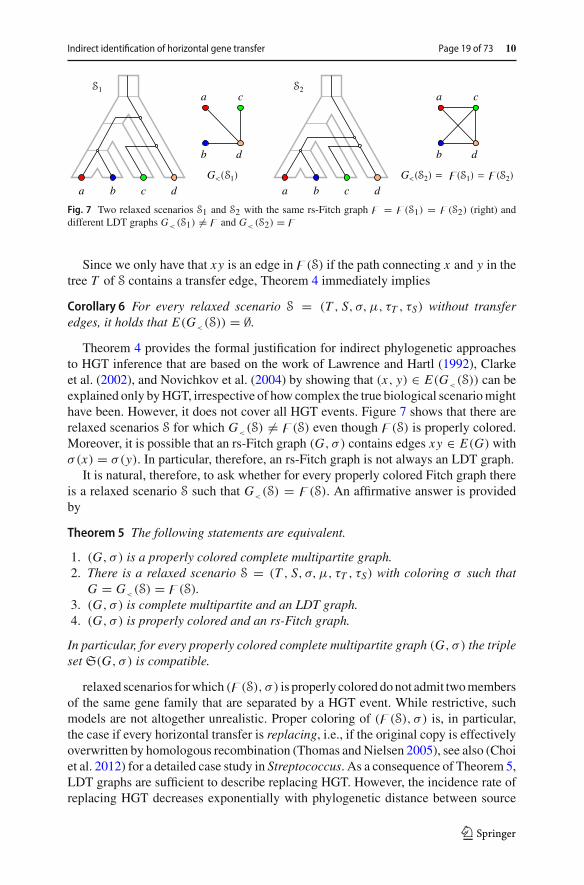
Fig. 7 Two relaxed scenarios S1 and S2 with the same rs-Fitch graph � = �(S1) = �(S2) (right) anddifferent LDT graphs G<(S1) �= � and G<(S2) = �
Since we only have that xy is an edge in �(S) if the path connecting x and y in thetree T of S contains a transfer edge, Theorem 4 immediately implies
Corollary 6 For every relaxed scenario S = (T , S, σ, μ, τT , τS) without transferedges, it holds that E(G<(S)) = ∅.
Theorem 4 provides the formal justification for indirect phylogenetic approachesto HGT inference that are based on the work of Lawrence and Hartl (1992), Clarkeet al. (2002), and Novichkov et al. (2004) by showing that (x, y) ∈ E(G<(S)) can beexplained only byHGT, irrespective of how complex the true biological scenariomighthave been. However, it does not cover all HGT events. Figure 7 shows that there arerelaxed scenarios S for which G<(S) �= �(S) even though �(S) is properly colored.Moreover, it is possible that an rs-Fitch graph (G, σ ) contains edges xy ∈ E(G) withσ(x) = σ(y). In particular, therefore, an rs-Fitch graph is not always an LDT graph.
It is natural, therefore, to ask whether for every properly colored Fitch graph thereis a relaxed scenario S such that G<(S) = �(S). An affirmative answer is providedby
Theorem 5 The following statements are equivalent.
1. (G, σ ) is a properly colored complete multipartite graph.2. There is a relaxed scenario S = (T , S, σ, μ, τT , τS) with coloring σ such that
G = G<(S) = �(S).3. (G, σ ) is complete multipartite and an LDT graph.4. (G, σ ) is properly colored and an rs-Fitch graph.
In particular, for every properly colored complete multipartite graph (G, σ ) the tripleset S(G, σ ) is compatible.
relaxed scenarios forwhich (�(S), σ ) is properly coloreddonot admit twomembersof the same gene family that are separated by a HGT event. While restrictive, suchmodels are not altogether unrealistic. Proper coloring of (�(S), σ ) is, in particular,the case if every horizontal transfer is replacing, i.e., if the original copy is effectivelyoverwritten by homologous recombination (Thomas andNielsen 2005), see also (Choiet al. 2012) for a detailed case study in Streptococcus. As a consequence of Theorem 5,LDT graphs are sufficient to describe replacing HGT. However, the incidence rate ofreplacing HGT decreases exponentially with phylogenetic distance between source
123

10 Page 20 of 73 D. Schaller et al.
and target (Williams et al. 2012), and additive HGT becomes the dominant mechanismbetween phylogenetically distant organisms. Still, replacing HGTs may also be theresult of additive HGT followed by a loss of the (functionally redundant) verticallyinherited gene.
5.3 rs-Fitch graphs with general colorings
In scenarios with additive HGT, the rs-Fitch graph is no longer properly colored andno-longer coincides with the LDT graph. Since not every vertex-colored completemultipartite graph (G, σ ) is an rs-Fitch graph (cf. Theorem 6), we ask whether an LDT(G, σ ) that is not itself already an rs-Fitch graph imposes constraints on the rs-Fitchgraphs (�(S), σ ) that derive from relaxed scenarios S that explain (G, σ ). As a firststep towards this goal, we aim to characterize rs-Fitch graphs, i.e., to understand theconditions imposed by the existence of an underlying scenario S on the compatibilityof the collection of independent setsI ofG and the coloring σ . As we shall see, theseconditions can be explained in terms of an auxiliary graph that we introduce in a verygeneral setting:
Definition 17 Let L be a set, σ : L → M a map andI = {I1, . . . , Ik} a set of subsetsof L . Then the graph A�(σ,I ) has vertex set M and edges xy if and only if x �= yand x, y ∈ σ(I ′) for some I ′ ∈ I .
By construction A�(σ,I ′) is a subgraph of A�(σ,I ) whenever I ′ ⊆ I . Anextended version of Definition 17 that contains also an edge-labeling of A�(σ,I )
can be found in the Technical Part—this technical detail is not needed here. As it turnsout, rs-Fitch graphs are characterized by the structure of their auxiliary graphs A� asshown in the next
Theorem 6 Agraph (G, σ ) is an rs-Fitch graph if and only if (i) it is completemultipar-tite with independent setsI = {I1, . . . , Ik}, and (ii) if k > 1, there is an independentset I ′ ∈ I such that A�(σ,I \{I ′}) is disconnected.
As a consequence of Theorem 6, we obtain
Corollary 9 rs-Fitch graphs can be recognized in polynomial time.
As for LDT graphs, the property of being an rs-Fitch graph is hereditary.
Corollary 14 If (G = (L, E), σ ) is an rs-Fitch graph, then the colored vertex inducedsubgaph (G[W ], σ|W ) is an rs-Fitch graph for all non-empty subsets W ⊆ L.
Note, however, that Corollary 14 is not satisfied if we restrict the codomain of σ
to the observable part of colors, i.e., if we consider σ|W ,σ (W ) : W → σ(W ) instead ofσ|W : W → M , even if σ is surjective. To see this consider the vertex colored graph(G, σ )with V (G) = {a, a′, b}, E(G) = {aa′, ab, a′b} and σ : V (G) → M = {A, B}where σ(a) = σ(a′) = A �= σ(b) = B. A possible relaxed scenario S for (G, σ )
is shown in Fig. 8A. The deletion of b yields W = V (G)\{b} = {a, a′} and thegraph (G[W ], σ|W ) for which S′ with HGT-labeling λS′ as in Fig. 8B is a relaxedscenario that satisfies G[W ] = �(T , λS′). However, if we restrict the codomain of
123

Indirect identification of horizontal gene transfer Page 21 of 73 10
A B C
Fig. 8 Shown are three distinct relaxed scenarios S, S′ and S′′ with corresponding rs-Fitch graphs. Hereσ ′ = σ|{a,a′} and σ ′′ = σ|{a,a′},{A} (cf. Definition 1). Putting (G, σ ) = (�(S), σ ), one can observe that(G[{a, a′}], σ ′) = (�(S′), σ ′) is an rs-Fitch graph. In contrast, σ ′′ is restricted to the “observable” part ofspecies (consisting of A alone), and (G[{a, a′}], σ ′′) is not an rs-Fitch graph, see text for further details
σ to obtain σ|W ,{A} : {a, a′} → σ(W ) = {A}, then there is no relaxed scenario S forwhich G[W ] = �(T , λS), since there is only a single species tree S on L(S) = {A}(Fig. 8C) that consists of the single edge (0T , A) and thus, μ(v) and μ(a) as well asμ(v) and μ(a′) must be comparable in this scenario.
5.4 Least resolved trees for Fitch graphs
It is important to note that the characterization of rs-Fitch graphs in Theorem 6 doesnot provide us with a characterization of rs-Fitch graphs that share a common relaxedscenario with a given LDT graph. As a potential avenue to address this problem weinvestigate the structure of least-resolved trees for Fitch graphs as possible source ofadditional constraints.
Definition 18 The edge-labeled tree (T , λ) is Fitch-least-resolved w.r.t. �(T , λ), iffor all trees T ′ �= T that are displayed by T and every labeling λ′ of T ′ it holds that�(T , λ) �= �(T ′, λ′).
As shown in the Technical Part (Theorem 7), Fitch-least-resolved trees can be char-acterized in terms of their edge-labeling, a result that is very similar to the results for“directed” Fitch graphs of 0/1-edge-labeled trees in Geiß et al. (2018). As a con-sequence of this characterization, Fitch-least-resolved trees can be constructed inpolynomial time. However, Fitch-least-resolved trees are far from being unique. Inparticular, Fitch-least-resolved trees are only of very limited use for the constructionof relaxed scenarios S = (T , S, σ, μ, τT , τS) from an underlying Fitch graph. In fact,even though (G, σ ) is an rs-Fitch graph, Example 3 in the Technical Part shows that it ispossible that there is no relaxed scenario S = (T , S, σ, μ, τT , τS) with HGT-labelingλS such that (T , λ) = (T , λS) for any of its Fitch-least-resolved trees (T , λ).
123

10 Page 22 of 73 D. Schaller et al.
6 Editing problems
6.1 Editing colored graphs to LDT graphs and Fitch graphs
Empirical estimates of LDT graphs from sequence data are expected to suffer fromnoise and hence to violate the conditions of Theorem 3. It is of interest, therefore, toconsider the problem of correcting an empirical estimate (G, σ ) to the closest LDTgraph. We therefore briefly investigate the usual three edge modification problems forgraphs: completion only considers the insertion of edges, for deletion edges may onlybe removed, while solutions to the editing problem allow both insertions and deletions,see e.g. Burzyn et al. (2006).
Problem 1 (LDT- Graph- Modification (LDT- M))
Input: A colored graph (G = (V , E), σ ) and an integer k.Question: Is there a subset F ⊆ E such that |F | ≤ k and (G ′ = (V , E�F), σ ) is an
LDT graph where � ∈ {\,∪,Δ}?We write LDT- E, LDT- C, LDT- D for the editing, completion, and deletion ver-
sion of LDT- M. By virtue of Theorem 3, the LDT- M is closely related to the problemof finding a compatible subset R ⊆ S(GR, σ ) with maximum cardinality. The cor-responding decision problem,MaxRTC, is known to be NP-complete (Jansson 2001,Thm. 1). In the technical part we prove
Theorem 9 LDT- M is NP-complete.
Even through at present it remains unclear whether rs-Fitch graphs can be estimateddirectly, the corresponding graph modification problems are at least of theoreticalinterest.
Problem 2 (rs- Fitch Graph- Modification (rsF- M))
Input: A colored graph (G = (V , E), σ ) and an integer k.Question: Is there a subset F ⊆ E such that |F | ≤ k and (G ′ = (V , E�F), σ ) is an
rs-Fitch graph where � ∈ {\,∪,Δ}?As above, wewrite rsF- E, rsF- C, rsF- D for the editing, completion, and deletion
version of rsF- M. Since rs-Fitch graphs are complete multipartite, their complementsare disjoint unions of complete graphs. The problems rsF- M are thus closely relatedthe cluster graph modification problems. Both Cluster Deletion and Cluster
Editing are NP-complete, while Cluster Completion is polynomial (by com-pleting each connected component to a clique, i.e., computing the transitive closure)(Shamir et al. 2004). We obtain
Theorem 10 rsF- C and rsF- E are NP-complete.
rsF- D remains open since the complement of the transitive closure of the complementof a colored graph (G, σ ) is not necessarily an rs-Fitch graph. This is in particular thecase if (G, σ ) is complete multipartite but not an rs-Fitch graph.
123
Indirect identification of horizontal gene transfer Page 23 of 73 10
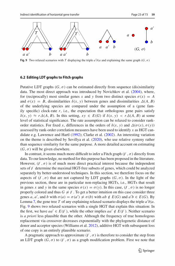
Fig. 9 Two relaxed scenarios with T displaying the triple a′b|a and explaining the same graph (G, σ )
6.2 Editing LDT graphs to Fitch graphs
Putative LDT graphs (G, σ ) can be estimated directly from sequence (dis)similaritydata. The most direct approach was introduced by Novichkov et al. (2004), where,for (reciprocally) most similar genes x and y from two distinct species σ(x) = Aand σ(x) = B, dissimilarities δ(x, y) between genes and dissimilarities Δ(A, B)
of the underlying species are compared under the assumption of a (gene fam-ily specific) clock-rate r , i.e., the expectation that orthologous gene pairs satisfyδ(x, y) ≈ rΔ(A, B). In this setting, xy ∈ E(G) if δ(x, y) < rΔ(A, B) at somelevel of statistical significance. The rate assumption can be relaxed to consider rank-order statistics. For fixed x , differences in the orders of δ(x, y) and Δ(σ(x), σ (y))assessed by rank-order correlation measures have been used to identify x as HGT can-didate e.g. Lawrence and Hartl (1992); Clarke et al. (2002). An interesting variationon the theme is described by Sevillya et al. (2020), who use relative synteny ratherthan sequence similarity for the same purpose. A more detailed account on estimating(G, σ ) will be given elsewhere.
In contrast, it seems much more difficult to infer a Fitch graph (�, σ ) directly fromdata. To our knowledge, nomethod for this purpose has been proposed in the literature.However, (�, σ ) is of much more direct practical interest because the independentsets of � determine the maximal HGT-free subsets of genes, which could be analyzedseparately by better-understood techniques. In this section, we therefore focus on theaspects of (�, σ ) that are not captured by LDT graphs (G, σ ). In the light of theprevious section, these are in particular non-replacing HGTs, i.e., HGTs that resultin genes x and y in the same species σ(x) = σ(y). In this case, (�, σ ) is no longerproperly colored and thus G �= �. To get a better intuition on this case consider threegenes a, a′, and b with σ(a) = σ(a′) �= σ(b) with ab /∈ E(G) and a′b ∈ E(G). ByLemma 7, the gene tree T of any explaining relaxed scenario displays the triple a′b|a.Fig. 9 shows two relaxed scenarios with a single HGT that explain this situation: Inthe first, we have aa′ ∈ E(�), while the other implies aa′ /∈ E(�). Neither scenariois a priori less plausible than the other. Although the frequency of true homologousreplacement via crossover decreases exponentially with the phylogenetic distance ofdonor and acceptor species (Williams et al. 2012), additive HGT with subsequent lossof one copy is an entirely plausible scenario.
A pragmatic approach to approximate (�, σ ) is therefore to consider the step froman LDT graph (G, σ ) to (�, σ ) as a graph modification problem. First we note that
123

10 Page 24 of 73 D. Schaller et al.
Algorithm 1 explicitly produces a relaxed scenario S and thus implies a correspondinggene tree TS with HGT-labeling λS, and thus an rs-Fitch graph (�(S), σ ). However,Algorithm 1 was designed primarily as proof device. It produces neither a uniquerelaxed scenario nor necessarily the most plausible or a most parsimonious one.Furthermore, both the LDT graph (G, σ ) and the desired rs-Fitch graph (�, σ ) areconsistent with a potentially very large number of scenarios. It thus appears preferableto altogether avoid the explicit construction of scenarios at this stage.
Since everyLDTgraph (G, σ ) is explained by someS, it is also a spanning subgraphof the corresponding rs-Fitch graph (�(S), σ ). The step from an LDT graph (G, σ )
to an rs-Fitch graph (�, σ ) can therefore be viewed as an edge-completion problem.The simplest variation of the problem is
Problem 3 (Fitch graph completion) Given an LDT graph (G, σ ), find a minimumcardinality set Q of possible edges such that ((V (G), E(G) ∪ Q), σ ) is a completemultipartite graph.
A close inspection of Problem 3 shows that the coloring is irrelevant in this version,and the actual problem to be solved is the problem Complete Multipartite Graph
Completionwith a cograph as input. We next show that this task can be performed inlinear time. The key idea is to consider the complementary problem, i.e., the problemof deleting a minimum set of edges from the complementary cograph G such that theend result is a disjoint union of complete graphs. This is known asCluster Deletion
problem (Shamir et al. 2004), and is known to have a greedy solution for cographs(Gao et al. 2013).
Lemma 18 There is a linear-time algorithm to solve Problem 3 for every cograph G.
All maximum clique partitions of a cograph G have the same sequence of cluster sizes(Gao et al. 2013, Thm. 1). However, they are not unique as partitions of the vertexset V (G). Thus the minimal editing set Q that needs to be inserted into a cograph toreach a complete multipartite graphs will not be unique in general. In the TechnicalPart, we briefly sketch a recursive algorithm operating on the cotree of G.
However, an optimal solution to Problem 3 with input (G, σ ) does not necessarilyyield an rs-Fitch graph or an rs-Fitch graph (�(S), σ ) such that G = G<(S), seeFig. 10. In particular, there are LDT graphs (G, σ ) for which more edges need to beadded to obtain an rs-Fitch graph than the minimum required to obtain a completemultipartite graph, see Fig. 11.
A more relevant problems for our purposes, therefore is
Problem 4 (rs-Fitch graph completion) Given an LDT graph (G, σ ) find a minimumcardinality set Q of possible edges such that ((V (G), E(G) ∪ Q), σ ) is an rs-Fitchgraph.
The following, stronger version is what we ideally would like to solve:
Problem 5 (strong rs-Fitch graph completion) Given an LDT graph (G, σ ) find aminimum cardinality set Q of possible edges such that � = ((V (G), E(G) ∪ Q), σ )
is an rs-Fitch graph and there is a common relaxed scenario S, that is, S satisfiesG = G<(S) and � = �(S).
123

Indirect identification of horizontal gene transfer Page 25 of 73 10
Fig. 10 Upper panel: A relaxed scenario Swith LDT graph (G<(S), σ ) and rs-Fitch graph (�(S), σ ). Thereare two minimum edge completion sets that yield the complete multipartite graphs (�1, σ ) and (�2, σ )
(lower part). By Theorem 6, (�2, σ ) is not an rs-Fitch graph. The graph (�1, σ ) is an rs-Fitch graph forthe relaxed scenario S′. However, G<(S) �= G<(S′) for all scenarios S′ with (�(S′), σ ) = (�1, σ ). To seethis, note that the gene tree T = ((a, b), (a′, b′)) in S is uniquely determined by application of Lemma 5and 7. Assume that there is any edge-labeling λ such that �(T , λ) = �1. The none-edges in �1 imply thatalong the two paths from a to a′ and b to b′ there is no transfer edge, that is, there cannot be any transferedge in T ; a contradiction
Fig. 11 The LDT graph (G<(S), σ ) for the relaxed scenario S has a unique minimum edge completionset (as determined by full enumeration), resulting in the complete multipartite graph (�1, σ ). However,Theorem 6 implies that (�1, σ ) is not rs-Fitch graph. An edge completion set with more edges must beused to obtain an rs-Fitch graph, for instance (�2, σ ), which is explained by the scenario S′
The computational complexity of Problems 4 and 5 is unknown. We conjecture,however, that both are NP-hard. In contrast to the application of graph modificationproblems to correct possible errors in the originally estimated data, the minimizationof inserted edges into an LDT graph lacks a direct biological interpretation. Instead,most-parsimonious solutions in terms of evolutionary events are usually of interest inbiology. In our framework, this translates to
Problem 6 (Min transfer completion) Let (G, σ ) be an LDT graph and S be the setof all relaxed scenarios S with G = G<(S). Find a relaxed scenario S′ ∈ S that hasa minimal number of transfer edges among all elements in S and the correspondingrs-Fitch graph �(S′).
123

10 Page 26 of 73 D. Schaller et al.
One way to address this problem might be as follows: Find edge-completion setsfor the given LDT graph (G, σ ) that minimize the number of independent sets inthe resulting rs-Fitch graph � = ((V (G), E(G) ∪ Q), σ ). The intuition behind thisidea is that, in this case, the number of pairs within the individual independent setsis maximized and thus, we get a maximized set of gene pairs without transfer alongtheir connecting path in the gene tree. It remains an open question whether this ideaalways yields a solution for Problem 6.
7 Simulation results
Evolutionary scenarios covering a wide range of HGT frequencies were generatedwith the simulation library AsymmeTree (Stadler et al. 2020). The tool generatesa planted species tree S with time map τS . A constant-rate birth-death process thengenerates a gene tree (T , τT ) with additional branching events producing copies atinner vertex u of S propagating to each descendant lineage of u. Tomodel HGT events,a recipient branch of S is selected at random. The simulation is event-based in the sensethat each node of the “true” gene tree other than the planted root is one of speciation,gene duplication, horizontal gene transfer, gene loss, or a surviving gene. Here, thelost as well as the surviving genes form the leaf set of T .
We used the following parameter settings for AsymmeTree: Planted species treeswith a number of leaves between 10 and 50 (randomly drawn in each scenario)were generated using the Innovation Model (Keller-Schmidt and Klemm 2012) andequipped with a time map as described in Stadler et al. (2020). Multifurcations wereintroduced into the species tree by contraction of inner edges with a common proba-bility p = 0.2 per edge to simulate. Gene trees therefore are also not binary in general.We usedmultifurcations tomodel the effects of limited phylogenetic resolution. Dupli-cation and HGT events, however, always result in bifurcations in the gene tree T . Weconsidered different combinations of duplication, loss, and HGT event rates (indicatedon the horizontal axis in Figs. 12, 13 and 14). For each combination of event rates,we simulated 1000 scenarios per event rate combination. Figure 12 summarizes basicstatistics of the simulated data sets.
The simulation also determines the set of surviving genes L ⊆ L(T ), the reconcil-iation map μ : V (T ) → V (S) ∪ E(S) and the coloring σ : L → L(S) representingthe species in which each surviving gene resides. From the true tree T , the observablegene tree T = T|L is obtained by recursively removing leaves that correspond to lossevents, i.e. L(T )\L , and suppressing inner vertices with a single child and settingτT (x) = τT (x) and μ(x) = μ(x) for all x ∈ V (T ). This defines a relaxed scenarioS = (T , S, σ, μ, τT , τS). From the scenario S, we can immediately determine theassociated HGT map λS, the Fitch graph �(S), and the LDT graph G<(S). We alsoconsider S = (T , S, σ, μ, τT , τS) which, from a formal point of view, is not a relaxedscenario, see Fig. 13. In this example, the gene-species association σ : L → L(S)
is not a map for the entire leaf set L(T ). Still, we can define the true LDT graphG< (S) and the true Fitch graph �(S) of S in the same way as LDT graphs usingDefinitions 8, 9, and 16, respectively. Note that this does not guarantee that every trueFitch graph is also an rs-Fitch graph. The example in Fig. 13 shows, furthermore,
123

Indirect identification of horizontal gene transfer Page 27 of 73 10
Fig. 12 Top panel: Distribution of the numbers of species (i.e. species tree leaves), species thereof thatcontain at least one surviving genes, surviving genes in total (non-loss leaves in the gene trees), loss events(loss leaves), and horizontal transfer events (inner vertices that are HGT events). Bottom panel: Mean andstandard deviation of these quantities. The numbers in the legend indicate the mean and standard deviationtaken over all event rate combinations. The tuples on the horizontal axis give the rates for duplication, loss,and horizontal transfer
Fig. 13 Left: Fraction of “visible” transfer edges among the “true” transfer edges in T in the simulatedscenarios, i.e., the edges that correspond to a path in T containing at least one transfer edge w.r.t. S (seealso the explanation in the text). The tuples on the horizontal axis give the rates for duplication, loss, andhorizontal transfer. Since E := E(�(S)) ⊆ E := E(�(S)[L(T )]), we also show the ratio |E |/|E |. Right:A relaxed scenario S = (T , S, σ, μ, τT , τS) with an “invisible” transfer edge (u, a′) (as determined by theknowledge of S = (T , S, σ, μ, τT , τS)). In this example we have �(S)[L(T ) = {a, a′}] �= �(S)
that �(S)[L] �= �(S) is possible. For the LDT graphs, on the other hand, we haveG<(S) = G< (S) because S and S are based on the same time maps.
The distinction between the true graph �(S)[L] and the rs-Fitch graph �(S) isclosely related to the definition of transfer edges. So far, we only took into accounttransfer edges (u, v) in the (observable) gene trees T , for which u and v are mappedto incomparable vertices or edges of the species trees S (cf. Definition 14). Thus,
123

10 Page 28 of 73 D. Schaller et al.
given the knowledge of the relaxed scenario S = (T , S, σ, μ, τT , τS), these transferedges are in that sense “visible”. However, given S = (T , S, σ, μ, τT , τS), which stillcontains all loss branches, it is possible that a non-transfer edge in T corresponds to apath in T which contains a transfer edge w.r.t. S, i.e., some edge (u, v) ∈ E(T ) suchthat μ(u) and μ(v) are incomparable in S. In particular, this is the casewhenever a geneis transferred into some recipient branch followed by a back-transfer into the originalbranch and a loss in the recipient branch (see Fig. 13, right). Figure 13 shows that,in the majority of the simulated scenarios, the HGT information is preserved in theobservable data. In fact, �(S) = �(S) in 86.7% of simulated scenarios. Occasionally,however, we also encounter scenarios in which large fractions of the xenologous pairsare hidden from inference by the LDT-based approach.
In the following, we will only be concerned with estimating a Fitch graph �(S),i.e., the graph resulting from the “visible” transfer edges. These were edgeless in about17.7% of the observable scenarios S (all parameter combinations taken into account).In these cases the LDT and thus also the inferred Fitch graphs are edgeless. Thesescenarios were excluded from further analysis.
We first ask how well the LDT graph G<(S) approximates the Fitch graph �(S).As shown in Fig. 14, the recall is limited. Over a broad range of parameters, the LDTgraph contains about a third of the xenologous pairs. This begs the question whetherthe solution of the editing Problem 3, obtained using the exact recursive algorithmdetailed in Sect. C in the Technical Part, leads to a substantial improvement. We findthat recall indeed increases substantially, at verymoderate levels of false positives. Theediting approach achieves a median precision of well above 90% in most cases and amedian recall of at least 60%, it provides results that are at the very least encouraging.We find that minimal edge completion (Problem 3) already yields an rs-Fitch graphin the vast majority of cases (99.8%, scenarios of all parameter combinations takeninto account), even if we restrict the color set to M ′ := σ(L) (instead of L(S)) andthus force surjectivity of the coloring σ . We note that the original LDT graph and theminimal edge completion may not always be explained by a common scenario. Thissuggests that it will be worthwhile to consider the more difficult editing problems forrs-Fitch graphs with a relaxed scenario S that at the same time explains the LDT graph.
Algorithm 1 provides a means to obtain an rs-Fitch graph satisfying the latter con-straint but without giving any guarantees for optimality in terms of a minimal edgecompletion.An implementation is available in the current release of theAsymmeTreepackage. For the rs-Fitch graphs �(S′) of the scenarios S′ constructed by Algorithm 1with (G<(S), σ ) as input, we observe another moderate increase of recall when com-pared with the minimal edge completion results. This comes, however, at the expenseof a loss in precision. This is not surprising, since �(S′) by construction contains atleast as many edges as any minimal edge completion ofG<(S). Therefore, the numberof both true positive and false positive edges in �(S′) can be expected to be higher,resulting in a higher recall and lower precision, respectively.
The recall is given by T P/(T P + FN ), and |E(�(S))| = T P + FN in terms oftrue positives T P and false negatives FN . Moreover,G<(S) is a subgraph of the Fitchgraphs �m.e.c. and �(S′) inferred with editing or with Algorithm 1, respectively. Theratio |E(�(S))∩E(�∗)|/|E(�(S)∩E(G<(S)))|with�
∗ ∈ {�m.e.c., �(S′)} thereforedirectly measures the increase in the number of correctly predicted xenologous pairs
123

Indirect identification of horizontal gene transfer Page 29 of 73 10
Fig. 14 Xenologs inferred from LDT graphs. Only observable scenarios S whose LDT graph (G<(S), σ )
contains at least one edge are included (82.3% of all scenarios). The tuples on the horizontal axis give therates for duplication, loss, and horizontal transfer. Top panel: Recall. Fraction of edges in �(S) representedin G<(S) (light blue). As an alternative, the fraction of edges in a “minimum edge completion” (m.e.c.) tothe “closest” complete multipartite graph is shown in dark blue. We observe a substantial increase in thefraction of inferred edges. The Fitch graph �(S′) obtained from the scenario S′ produced by Algorithm 1with input (G<(S), σ ) yields an even better recall (light green). Second panel: Increase in the number ofcorrectly inferred edges relative to the LDT graphG<(S). Third panel: Precision. In contrast to LDT graphs,which by Theorem 4 cannot contain false positive edges, this is not the case for the estimated Fitch graphsobtained as m.e.c. and by Algorithm 1. While false positive edges are typically rare, occasionally very poorestimates are observed. Bottom panel: Accuracy
relative to theLDT. It is equivalent to the ratio of the respective recalls. By construction,the ratio is always ≥ 1. This is summarized as the second panel in Fig. 14.
8 Discussion and future directions
In this contribution, we have introduced later-divergence-time (LDT) graphs as amodel capturing the subset of horizontal transfer detectable through the pairs of genes
123

10 Page 30 of 73 D. Schaller et al.
that have diverged later than their respective species. Within the setting of relaxed sce-narios, LDT graphs (G, σ ) are exactly the properly colored cographs with a consistenttriple set S(G, σ ). We further showed that LDT graphs describe a sufficient set ofHGT events if and only if they are complete multipartite graphs. This corresponds toscenarios in which all HGT events are replacing. Otherwise, additional HGT eventsexist that separate genes from the same species. To better understand these, we inves-tigated scenario-derived rs-Fitch graphs and characterized them as those completemultipartite graphs that satisfy an additional constraint on the coloring (expressed interms of an auxiliary graph). Although the information contained in LDT graphs isnot sufficient to unambiguously determine the missing HGT edges, we arrive at anefficiently solvable graph editing problem from which a “best guess” can be obtained.To our knowledge, this is the first detailed mathematical investigation into the powerand limitation of an implicit phylogenetic method for HGT inference.
From a data analysis point of view, LDT graphs appear to be an attractive avenue toinfer HGT in practice. While existing methods to estimate them from (dis)similaritydata certainly can be improved, it is possible to use their cograph structure to correctthe initial estimate in the same way as orthology data (Hellmuth et al. 2015). Althoughthe LDT modification problems are NP-complete (Theorem 9), it does not appear toodifficult to modify efficient cograph editing heuristics (Crespelle 2019; Hellmuth et al.2020a) to accommodate the additional coloring constraints.
LDT graphs by themselves clearly do no contain sufficient information to com-pletely determine a relaxed scenario. Additional information, e.g. a best match graph(Geiß et al. 2019, 2020a) will certainly be required. The most direct practical use ofLDT information is to infer the Fitch graph, whose independent sets correspond tomaximal HGT-free subsets of genes. These subsets can be analyzed separately (Hell-muth 2017) using recent results to infer gene family histories, including orthologyrelations from best match data (Geiß et al. 2020a; Schaller et al. 2021b). The mainremaining unresolved question is whether the resultingHGT-free subtrees can be com-bined into a complete scenario using only relational information such as best matchdata. One way to attack this is to employ the techniques used by Lafond and Hellmuth(2020) to characterize the conditions under which a fully event-labled gene tree can bereconciled with unknown species trees. These not only resulted in an polynomial-timealgorithm but also establishes additional constraints on the HGT-free subtrees. Analternative, albeit mathematically less appealing approach is to adapt classical phy-logenetic methods to accommodate the HGT-free subtrees as constraints. We suspectthat best match data can supply further, stringent constraints for this task. We willpursue this avenue elsewhere.
Several alternative routes can be followed to obtain Fitch graphs from LDT graphs.The most straightforward approach is to elaborate on the editing problems brieflydiscussed in Sect. 6. A natural question arising in this context is whether there arenon-LDT edges that are shared by all minimal completion sets Q, and whether these“obligatory Fitch-edges” can be determined efficiently. A natural alternative is tomod-ify Algorithm 1 to incorporate some form of cost function to favor the construction ofbiologically plausible scenarios. In a very different approach, one might also considerto use LDT graphs as constraints in probabilistic models to reconstruct scenarios, seee.g. Sjöstrand et al. (2014) and Khan et al. (2016).
123

Indirect identification of horizontal gene transfer Page 31 of 73 10
Although we have obtained characterizations of both LDT graphs and rs-Fitchgraphs, many open questions and avenues for future research remain.Reconciliation maps The notion of relaxed reconciliation maps used here appearsto be at least as general as alternatives that have been explored in the literature. Itavoids the concurrent definition of event types and thus allows situations that may beexcluded in a more restrictive setting. For example, relaxed scenarios may have twoor more vertically inherited genes x and y in the same species with u := lcaT (x, y)mapping to a vertex of the species trees. In the usual interpretation, u correspond to aspeciation event (by virtue ofμ(u) ∈ V 0(S)); on the other hand, the descendants x andy constitute paralogs in most interpretations. Such scenarios are explicitly excludede.g. in Stadler et al. (2020). Lemma 3 suggests that relaxed scenarios are sufficientlyflexible to make it possible to replace a scenario S that is “forbidden” in responseto such inconsistent interpretations of events by an “allowed” scenario S′ with thesame σ such that G<(S) = G<(S′). Whether this is indeed true, or whether a morerestrictive definition of reconciliation imposes additional constraints of LDT graphswill of course need to be checked in each case.
The restriction of aμ-free scenario to a subset L ′ of leaves of T and to a subsetM ′ ofleaves of S is well defined as long as σ(L ′) ⊆ M ′. One can also define a correspondingrestriction of the reconciliation map μ. Most importantly, the deletion of some leavesof T may leave inner vertices in T with only a single child, which are then suppressedto recover a phylogenetic tree. This replaces paths in T by single edges and thusaffects the definition of the HGT map λS since a path in T that contains two adjacentvertices u1, u2 with incomparable images μ(u1) and μ(u2) may be replaced by anedge with comparable end points in the restricted scenario S′. This means that HGTevents may become invisible, and thus �(S′) is not necessarily an induced subgraphof �(S), but a subgraph that may lack additional edges. Note that this is in contrast tothe assumptions made in the analysis of (directed) Fitch graphs of 0/1-edge-labeledgraphs (Geiß et al. 2018; Hellmuth and Seemann 2019), where the information onhorizontal transfers is inherited upon restriction of (T , λ).Observability The latter issue is a special case of the more general problem withobservability of events. Conceptually, we assume that evolution followed a true sce-nario comprising discrete events (speciations, duplications, horizontal transfer, genelosses, and possibly other events such as hybridization which are not considered here).In computer simulations, of course we know this true scenario, as well as all eventtypes. Gene loss not only renders some leaves invisible but also erases the evidenceof all subtrees without surviving leaves. Removal of these vertices in general resultsin a non-phylogenetic gene tree that contains inner vertices with a single child. In theabsence of horizontal transfer, this causes little problems and the unobservable verticescan be be removed as described in the previous paragraph, see e.g. Hernández-Rosaleset al. (2012). The situation ismore complicatedwithHGT. InNøjgaard et al. (2018), anHGT-vertex is deemed observable if it has both a horizontally and a vertically inher-ited descendant. In our present setting, the scenario retains an HGT-edge by virtueof consecutive vertices in T with incomparable μ-images, irrespective of whether anHGT-vertex is retained. This type of “vertex-centered” notion of xenology is exploredfurther in Hellmuth et al. (2017). We suspect that these different points of view canbe unified only when gene losses are represented explicitly or when gene and species
123
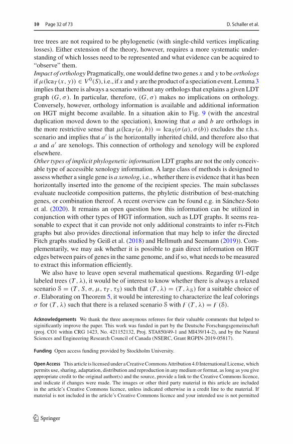
10 Page 32 of 73 D. Schaller et al.
tree trees are not required to be phylogenetic (with single-child vertices implicatinglosses). Either extension of the theory, however, requires a more systematic under-standing of which losses need to be represented and what evidence can be acquired to“observe” them.Impact of orthology Pragmatically, onewould define two genes x and y to be orthologsifμ(lcaT (x, y)) ∈ V 0(S), i.e., if x and y are the product of a speciation event. Lemma3implies that there is always a scenario without any orthologs that explains a given LDTgraph (G, σ ). In particular, therefore, (G, σ ) makes no implications on orthology.Conversely, however, orthology information is available and additional informationon HGT might become available. In a situation akin to Fig. 9 (with the ancestralduplication moved down to the speciation), knowing that a and b are orthologs inthe more restrictive sense that μ(lcaT (a, b)) = lcaS(σ (a), σ (b)) excludes the r.h.s.scenario and implies that a′ is the horizontally inherited child, and therefore also thata and a′ are xenologs. This connection of orthology and xenology will be exploredelsewhere.Other types of implicit phylogenetic information LDT graphs are not the only conceiv-able type of accessible xenology information. A large class of methods is designed toassess whether a single gene is a xenolog, i.e., whether there is evidence that it has beenhorizontally inserted into the genome of the recipient species. The main subclassesevaluate nucleotide composition patterns, the phyletic distribution of best-matchinggenes, or combination thereof. A recent overview can be found e.g. in Sánchez-Sotoet al. (2020). It remains an open question how this information can be utilized inconjunction with other types of HGT information, such as LDT graphs. It seems rea-sonable to expect that it can provide not only additional constraints to infer rs-Fitchgraphs but also provides directional information that may help to infer the directedFitch graphs studied by Geiß et al. (2018) and Hellmuth and Seemann (2019)). Com-plementarily, we may ask whether it is possible to gain direct information on HGTedges between pairs of genes in the same genome, and if so, what needs to bemeasuredto extract this information efficiently.
We also have to leave open several mathematical questions. Regarding 0/1-edgelabeled trees (T , λ), it would be of interest to know whether there is always a relaxedscenario S = (T , S, σ, μ, τT , τS) such that (T , λ) = (T , λS) for a suitable choice ofσ . Elaborating on Theorem 5, it would be interesting to characterize the leaf coloringsσ for (T , λ) such that there is a relaxed scenario S with �(T , λ) = �(S).
Acknowledgements We thank the three anonymous referees for their valuable comments that helped tosiginificantly improve the paper. This work was funded in part by the Deutsche Forschungsgemeinschaft(proj. CO1 within CRG 1423, No. 421152132, Proj. STA850/49-1 and MI439/14-2), and by the NaturalSciences and Engineering Research Council of Canada (NSERC, Grant RGPIN-2019-05817).
Funding Open access funding provided by Stockholm University.
OpenAccess This article is licensedunder aCreativeCommonsAttribution 4.0 InternationalLicense,whichpermits use, sharing, adaptation, distribution and reproduction in any medium or format, as long as you giveappropriate credit to the original author(s) and the source, provide a link to the Creative Commons licence,and indicate if changes were made. The images or other third party material in this article are includedin the article’s Creative Commons licence, unless indicated otherwise in a credit line to the material. Ifmaterial is not included in the article’s Creative Commons licence and your intended use is not permitted
123

Indirect identification of horizontal gene transfer Page 33 of 73 10
by statutory regulation or exceeds the permitted use, you will need to obtain permission directly from thecopyright holder. To view a copy of this licence, visit http://creativecommons.org/licenses/by/4.0/.
Technical part
A Later-divergence-time graphs
A.1 LDT graphs and evolutionary scenarios
In the absence of horizontal gene transfer, the last common ancestor of two species Aand B should mark the latest possible time point at which two genes a and b residingin σ(a) = A and σ(b) = B, respectively, may have diverged. Situations in which thisconstraint is violated are therefore indicative of HGT.
Definition 7 (μ-free scenario) Let T and S be planted trees, σ : L(T ) → L(S) be amap and τT and τS be time maps of T and S, respectively, such that τT (x) = τS(σ (x))for all x ∈ L(T ). Then, T = (T , S, σ, τT , τS) is called a μ-free scenario.
The condition that τT (x) = τS(σ (x)) for all x ∈ L(T ) is mostly a technical conve-nience thatmakesμ-free scenarios easier to interpret.Nevertheless, byLemma1, giventhe time map τS , one can easily construct a time map τT such that τT (x) = τS(σ (x))for all x ∈ L(T ). In particular, when constructing relaxed scenarios explicitly, wemaysimply choose τT (u) = 0 and τS(x) = 0 as common time for all leaves u ∈ L(T ) andx ∈ L(S).
Definition 8 (LDT graph) For a μ-free scenario T = (T , S, σ, τT , τS), we defineG<(T) = G<(T , S, σ, τT , τS) = (V , E) as the graph with vertex set V := L(T ) andedge set
E := {ab | a, b ∈ L(T ), τT (lcaT (a, b)) < τS(lcaS(σ (a), σ (b))).}
A vertex-colored graph (G, σ ) is a later-divergence-time graph (LDT graph), if thereis a μ-free scenario T = (T , S, σ, τT , τS) such that G = G<(T). In this case, we saythat T explains (G, σ ).
It is easy to see that the edge set of G<(T) defines an undirected graph and thatthere are no edges of the form aa, since τT (lcaT (a, a)) = τT (a) = τS(σ (a)) =τS(lcaS(σ (a), σ (a))). Hence G<(T) is a simple graph.
By definition, every relaxed scenario S = (T , S, σ, μ, τT , τS) satisfies τT (x) =τS(σ (x)) all x ∈ L(T ). Therefore, removing μ from S yields a μ-free scenario T =(T , S, σ, τT , τS). Thus, we will use the following simplified notation.
Definition 9 We put G<(S) := G<(T , S, σ, τT , τS) for a given relaxed scenario S =(T , S, σ, μ, τT , τS) and the underlying μ-free scenario (T , S, σ, τT , τS) and say, byslight abuse of notation, that S explains (G<(S), σ ).
Lemma 2 For everyμ-free scenario T = (T , S, σ, τT , τS), there is a relaxed scenarioS = (T , S, σ, μ, τT , τS) for T , S and σ such that (G<(T), σ ) = (G<(S), σ ).
123

10 Page 34 of 73 D. Schaller et al.
Proof Let T = (T , S, σ, τT , τS) be a μ-free scenario. In order to construct a relaxedscenario S = (T , S, σ, μ, τT , τS) that satisfies G<(S) = G<(T), we start with a timemap τT for T satisfying τT (0T ) = max(τT (0T ), τS(0S)) and τT (v) = τT (v) for allv ∈ V (T )\{0T }. Correspondingly,we introduce a timemap τS for S such that τS(0S) =max(τT (0T ), τS(0S)) and τS(v) = τS(v) for all v ∈ V (S)\{0S}. By construction, wehave tmax,T := max{τT (v) | v ∈ V (T )} = τT (0T ) = τS(0S). Moreover, we havetmin,S := min{τS(v) | v ∈ V (S)} ≤ min{τT (v) | v ∈ V (T )} =: tmin,T . To see this,we can choose x ∈ V (T ) such that τT (v) = tmin,T . By the definition of time maps andminimality of τT (v), the vertex x must be a leaf. Hence, since T is a μ-free scenario,we have τT (x) = τS(σ (x)) with X := σ(x) ∈ L(S) ⊂ V (S). Therefore, it musthold that tmin,S ≤ tmin,T . We now define P := {p ∈ V (S) ∪ E(S) | X S p}, i.e.,the set of all vertices and edges on the unique path in S from 0S to the leaf X . SinceτS(X) = tmin,T < tmax,T = τS(0S), we find, for each v ∈ V (T ), either a vertex u ∈ Psuch that τT (v) = τS(u) or an edge (u, w) ∈ P such that τS(w) < τT (v) < τS(u).Hence, we can specify the reconciliation map μ by defining, for every v ∈ V (T ),
μ(v) :=
⎧⎪⎪⎪⎨
⎪⎪⎪⎩
0S if v = 0T ,
σ (v) if v ∈ L(T ),
u if there is some vertex u ∈ P with τT (v) = τS(u),
(u, w) if there is some edge (u, w) ∈ P with τS(w) < τT (v) < τS(u).
For each v ∈ V 0(T ), exactly one of the two alternatives for P applies, hence μ iswell-defined. It is now an easy task to verify that all conditions in Definitions 4 and 5are satisfied for S = (T , S, σ, μ, τT , τS) by construction. Hence, by Definition 6, S isa relaxed scenario.
It remains to show that G<(T) = G<(S). Let a, b ∈ L(T ) be arbitrary. Clearly,neither lcaT (a, b) nor lcaS(σ (a), σ (b)) equals the planted root 0T or 0S , respec-tively. Since we have only changed the timing of the roots 0T or 0S , we obtain ab ∈E(G<(S)) if and only if τT (lcaT (a, b)) = τT (lcaT (a, b)) < τS(lcaS(σ (a), σ (b))) =τS(lcaS(σ (a), σ (b))) if and only if ab ∈ E(G<(T)), which completes the proof. ��
Theorem 1 (G, σ ) is an LDT graph if and only if there is a relaxed scenario S =(T , S, σ, μ, τT , τS) such that (G, σ ) = (G<(S), σ ).
Proof By definition, (G, σ ) is an LDT graph for every relaxed scenario S with col-oring σ that satisfies (G, σ ) = (G<(S), σ ). Now suppose that (G, σ ) is an LDTgraph. By definition, there is a μ-free scenario T = (T , S, σ, τT , τS) with color-ing σ such that (G, σ ) = (G<(T), σ ). By Lemma 2, there is a relaxed scenarioS = (T , S, σ, μ, τT , τS) for T , S and σ such that (G, σ ) = (G<(S), σ ). ��
Remark 3 From here on, we omit the explicit reference to Lemma 2 and Thm 1 andassume that the reader is aware of the fact that every LDT graph is explained by somerelaxed scenario S and that for every μ-free scenario T = (T , S, σ, τT , τS), there is arelaxed scenario S for T , S and σ such that (G<(T), σ ) = (G<(S), σ ).
123

Indirect identification of horizontal gene transfer Page 35 of 73 10
We now derive some simple properties of μ-free and relaxed scenarios. It may besurprising at first glance that “the speciation nodes”, i.e., vertices u ∈ V 0(T ) withμ(u) ∈ V (S) do not play a special role in determining LDT graphs.
Lemma 3 For every relaxed scenario S = (T , S, σ, μ, τT , τS) there exists a relaxedscenario S = (T , S, σ, μ, τT , τS) such that G< (S) = G<(S) and for all distinctx, y ∈ L(T ) with xy /∈ E(G<(S)) holds τT (lcaT (x, y)) > τS(lcaS(σ (x), σ (y))).
Proof For the relaxed scenario S = (T , S, σ, μ, τT , τS) we write V 0(S) :=V (S)\(L(S) ∪ {0S}) and define
DS := {|τS(y) − τS(x)| : x, y ∈ V (S), τS(x) �= τS(y)},DT := {|τT (y) − τT (x)| : x, y ∈ V (T ), τT (x) �= τT (y)}, andDT S := {|τT (x) − τS(y)| : x ∈ V (T ), y ∈ V (S), τT (x) �= τS(y)}.
We have DS �= ∅ and DT �= ∅ since we do not consider empty trees, and thus, at leastthe “planted” edges 0SρS and 0T ρT always exist. By construction, all values in DT ,DS , and DT S are strictly positive. Now define
ε := 1
2min(DST ∪ DS ∪ DT ).
Since DS and DT are not empty, ε is well-defined and, by construction, ε > 0. Nextwe set, for all v ∈ V (T ),
τT (v) :={
τT (v) + ε, if v ∈ V 0(T )
τT (v), otherwise,
μ(v) :={
(par(x), x), if μ(v) = x ∈ V 0(S)
μ(v), otherwise.
Claim 1 S := (T , S, σ, μ, τT , τS) is a relaxed scenario.
Proof By construction, if μ(v) ∈ (L(S) ∪ {0S}) and thus, μ(v) /∈ V 0(S), μ(v) andμ(v) coincide. Therefore, (G0) and (G1) are trivially satisfied for μ. In order to show(G2), we first note that τT (v) = τT (v) = τS(σ (v)) holds for all v ∈ L(T ) byDefinition 4.
We next argue that τT is a time map. To this end, let x, y ∈ V (T ) with x ≺T y.Hence, τT (x) < τT (y) and, in particular, τT (y)− τT (x) ≥ 2ε. Assume for contradic-tion that τT (x) ≥ τT (y). This implies τT (x) = τT (x) + ε and τT (y) = τT (y),since τT (x) < τT (y) and ε > 0 always implies τT (x) + ε < τT (y) + ε andτT (x) < τT (y) + ε. Therefore, τT (y) − τT (x) = τT (y) − (τT (x) + ε) ≥ ε > 0and thus, τT (y) > τT (x); a contradiction.
Wecontinuewith showing that the two timemaps τT and τS are time-consistentw.r.t.S. To see that Condition (C1) is satisfied, observe that, by construction, μ(v) ∈ V (S)
does hold only in case μ(v) /∈ E(S) ∪ V 0(S) and thus, μ(v) ∈ L(S) ∪ {0S}. In this
123
10 Page 36 of 73 D. Schaller et al.
case, μ(v) = μ(v) and since μ(v) satisfies (G1) we have v ∈ L(T ) ∪ {0T }. Thus,v /∈ V 0(T ) and, therefore, τT (v) = τT (v) = τS(μ(v)). Therefore, Condition (C1) issatisfied.
Now consider Condition (C2). As argued above, μ(v) ∈ E(S) holds for all v ∈V 0(T ) = V (T )\(L(T ) ∪ {0T }). By construction, τT (v) = τT (v) + ε. There are twocases: μ(v) = x ∈ V 0(S), or μ(v) = (y, x) ∈ E(S) with y = par(x). The followingarguments hold for both cases: We have μ(v) = (y, x) ∈ E(S). Moreover, τS(x) ≤τT (v) < τT (v) since τT and τS satisfy (C1) and (C2). Furthermore, τT (v) < τS(y)and, by construction, τS(y) − τT (v) ≥ 2ε. This immediately implies that τS(y) ≥τT (v) + 2ε = τT (v) + ε > τT (v). In summary, τS(x) < τT (v) < τS(y) wheneverμ(v) = (y, x) ∈ E(S). Therefore, Condition (C2) is satisfied for S. �Claim 2 E(G<(S)) ⊆ E(G< (S)).
Proof Let xy be an edge in G<(S) and thus x �= y, and set vT := lcaT (x, y) andvS := lcaS(σ (x), σ (y)). By definition, we have τT (vT ) < τS(vS). Therefore, wehave τS(vS) − τT (vT ) ∈ DT S and, hence, τS(vS) − τT (vT ) ≥ 2ε. Since x �= y, vT =lcaT (x, y) is an inner vertex of T . By construction, therefore, τT (vT ) = τT (vT ) + ε.The latter arguments together with the fact that τS remains unchanged imply thatτS(vS) − τT (vT ) ≥ ε > 0, and thus, τT (vT ) < τS(vS). Therefore, we conclude thatxy is an edge in G< (S). �It remains to show
Claim 3 For all distinct x, y ∈ L(T ) with xy /∈ E(G<(S)), we have τT (lcaT (x, y)) >
τS(lcaS(σ (x), σ (y))).
Proof Suppose xy /∈ E(G<(S)) for twodistinct x, y ∈ L(T ), and set vT := lcaT (x, y)and vS := lcaS(σ (x), σ (y)). By definition, this implies τT (vT ) ≥ τS(vS). Sincex �= y, we clearly have that vT = lcaT (x, y) is an inner vertex of T , and hence,τT (vT ) = τT (vT ) + ε. The latter two argument together with ε > 0 and the fact thatτS remains unchanged imply that τT (vT ) > τS(vS). �In particular, therefore, xy /∈ E(G<(S)) implies that xy /∈ E(G< (S)) and therefore,E(G< (S)) ⊆ E(G<(S)). Together with Claim 2 and the fact that both G<(S) andG< (S) have vertex set L(T ), we conclude that G<(S) = G< (S), which completes theproof. ��
Since the relaxed scenario S = (T , S, σ, μ, τT , τS) as constructed in the proof ofLemma 3 satisfies μ(v) /∈ V 0(S) we obtain
Corollary 1 For every relaxed scenario S = (T , S, σ, μ, τT , τS) there exists a relaxedscenario S = (T , S, σ, μ, τT , τS) such that G< (S) = G<(S) and μ(v) /∈ V 0(S) forall v ∈ V (T ).
Lemma 3, however, does not imply that one can always find a relaxed scenariowith a reconciliation map μ for given trees T and S satisfying μ(lcaT (x, y)) �S
lcaS(σ (x), σ (y)) for all distinct x, y ∈ L(T ) with xy /∈ E(G<(S)), as shown inExample 2.
123
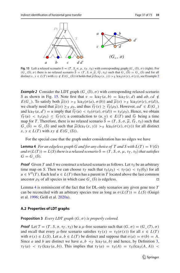
Indirect identification of horizontal gene transfer Page 37 of 73 10
Fig. 15 Left a relaxed scenario S = (T , S, σ, μ, τT , τS) with corresponding graph (G<(S), σ ) (right). For(G<(S), σ ) there is no relaxed scenario S = (T , S, σ, μ, τT , τS) such that G< (S) = G<(S) and for alldistinct x, y ∈ L(T )with xy /∈ E(G<(S)) it holds that μ(lcaT (x, y)) �S lcaS(σ (x), σ (y)), see Example 2
Example 2 Consider the LDT graph (G<(S), σ ) with corresponding relaxed scenarioS as shown in Fig. 15. Note first that v = lcaT (a, b) = lcaT (c, d) and ab, cd /∈E(G<). To satisfy both μ(v) �S lcaS(σ (a), σ (b)) and μ(v) �S lcaS(σ (c), σ (d)),we clearly need that μ(v) S ρS , and thus τT (v) ≥ τS(ρS). However, ad ′ ∈ E(G<)
and lcaT (a, d ′) = u imply that τT (u) < τS(σ (a), σ (d)) = τS(ρS). Hence, we obtainτT (u) < τS(ρS) ≤ τT (v); a contradiction to (u, v) ∈ E(T ) and τT being a timemap for T . Therefore, there is no relaxed scenario S = (T , S, σ, μ, τT , τS) such thatG< (S) = G<(S) and such that μ(lcaT (x, y)) �S lcaS(σ (x), σ (y)) for all distinctx, y ∈ L(T ) with xy /∈ E(G<(S)).
For the special case that the graph under consideration has no edges we have
Lemma 4 For an edgeless graph G and for any choice of T and S with L(T ) = V (G)
andσ(L(T )) = L(S) there is a relaxed scenarioS = (T , S, σ, μ, τT , τS) that satisfiesG = G<(S).
Proof Given T and S we construct a relaxed scenario as follows. Let τS be an arbitrarytime map on S. Then we can choose τT such that τS(ρS) < τT (u) < τS(0S) for allu ∈ V 0(T ). Each leaf u ∈ L(T ) then has a parent in T located above the last commonancestor ρS of all species in which case G<(S) is edgeless. ��Lemma 4 is reminiscent of the fact that for DL-only scenarios any given gene tree Tcan be reconciled with an arbitrary species tree as long as σ(L(T )) = L(S) (Guigóet al. 1996; Geiß et al. 2020a).
A.2 Properties of LDT graphs
Proposition 3 Every LDT graph (G, σ ) is properly colored.
Proof Let T = (T , S, σ, τT , τS) be a μ-free scenario such that (G, σ ) = (G<(T), σ )
and recall that every μ-free scenario satisfies τT (x) = τS(σ (x)) for all x ∈ L(T )
with σ(x) ∈ L(S). Let a, b ∈ L(T ) be distinct and suppose that σ(a) = σ(b) = A.Since a and b are distinct we have a, b ≺T lcaT (a, b) and hence, by Definition 3,τT (a) < τT (lcaT (a, b)). This implies that τT (a) = τS(A) = τS(lcaS(A, A)) <
123

10 Page 38 of 73 D. Schaller et al.
τT (lcaT (a, b)). Therefore, ab /∈ E(G). Consequently, ab ∈ E(G) implies σ(a) �=σ(b), which completes the proof. ��
Extending earlier work of Dekker (1986) and Bryant and Steel (1995) derivedconditions under which two triples r1, r2 imply a third triple r3 that must be displayedby any tree that displays r1, r2. In particular, we make frequent use of the following
Lemma 5 If a tree T displays xy|z and zw|y then T displays xy|w and zw|x. Inparticular T|{x,y,z,w} = ((x, y), (z, w)) (in Newick format).
Definition 10 For every graph G = (L, E), we define the set of triples on L
T(G) := {xy|z : x, y, z ∈ L are pairwise distinct, xy ∈ E, xz, yz /∈ E} .
If G is endowed with a coloring σ : L → M we also define a set of color triples
S(G, σ ) := {σ(x)σ (y)|σ(z) : x, y, z ∈ L, σ (x), σ (y), σ (z) are pairwise distinct,
xz, yz ∈ E, xy /∈ E}.
Lemma 6 If a graph (G, σ ) is an LDT graph then S(G, σ ) is compatible and SdisplaysS(G, σ ) for everyμ-free scenarioT = (T , S, σ, τT , τS) that explains (G, σ ).
Proof Suppose that (G = (L, E), σ ) is an LDT graph and let T = (T , S, σ, τT , τS)
be aμ-free scenario that explains (G, σ ). In order to show thatS(G, σ ) is compatibleit suffices to show that S displays every triple in S(G, σ ).
Let AB|C ∈ S(G, σ ). By definition, A, B,C are pairwise distinct and theremust be vertices a, b, c ∈ L with σ(a) = A, σ(b) = B, and σ(c) =C such that ab /∈ E and bc, ac ∈ E . First, ab /∈ E and bc, ac ∈ Eimply τT (lcaT (a, b)) ≥ τS(lcaS(A, B)), τT (lcaT (b, c)) < τS(lcaS(B,C)), andτT (lcaT (a, c)) < τS(lcaS(A,C)). Moreover, for any three vertices a, b, c in T itholds that 1 ≤ |{lcaT (a, b), lcaT (a, c), lcaT (b, c)}| ≤ 2.
Therefore we have to consider the following four cases: (1) u := lcaT (a, b) =lcaT (b, c) = lcaT (a, c), (2) u := lcaT (a, b) = lcaT (a, c) �= lcaT (b, c) and (3)u := lcaT (a, b) = lcaT (b, c) �= lcaT (a, c), (4) lcaT (a, b) �= u := lcaT (b, c) =lcaT (a, c). Note, for any three vertices x, y, z in T , lcaT (x, y) �= lcaT (x, z) =lcaT (y, z) implies that lcaT (x, y) ≺T lcaT (x, z) = lcaT (y, z). In Cases (1) and(2), we find τS(lcaS(A,C)) > τT (u) ≥ τS(lcaS(A, B)). Together with the fact thatlcaS(A,C) and lcaS(A, B) are comparable in S, this implies that AB|C is displayedby S. In Case (3), we obtain τS(lcaS(B,C)) > τT (u) ≥ τS(lcaS(A, B)) and, by anal-ogous arguments, AB|C is displayed by S. Finally, in Case (4), the tree T displaysthe triple ab|c. Thus, τS(lcaS(A, B)) ≤ τT (lcaT (a, b)) < τT (u) < τS(lcaS(A,C)).Again, AB|C is displayed by S. ��
The next lemma shows that induced K2 + K1 subgraphs in LDT graphs impliestriples that must be displayed by T .
Lemma 7 If (G, σ ) is an LDT graph, then T(G) is compatible and T displays T(G)
for every μ-free scenario T = (T , S, σ, τT , τS) that explains (G, σ ).
123

Indirect identification of horizontal gene transfer Page 39 of 73 10
Proof Suppose that (G = (L, E), σ ) is an LDT graph and let T = (T , S, σ, τT , τS)
be a μ-free scenario that explains (G, σ ). In order to show that T(G) is compatible itsuffices to show that T displays every triple in T(G, σ ).
Let ab|c ∈ T(G). By definition, a, b, c ∈ L(T ) are distinct, and ab ∈ E andac, bc /∈ E . Since ab ∈ E , we have A := σ(a) �= σ(b) =: B by Proposition 3.
There are two cases, either σ(c) ∈ {A, B} or not. Suppose first that w.l.o.g.σ(c) = A. In this case, ab ∈ E and bc /∈ E together imply τT (lcaT (a, b)) <
τS(lcaS(A, B)) ≤ τT (lcaT (b, c)). This and the fact that lcaT (a, b) and lcaT (b, c) arecomparable in T implies that T displays ab|c.
Suppose now that σ(c) = C /∈ {A, B}. We now consider the four possible topolo-gies of S′ = S|ABC : (1) S′ is a star, (2) S′ = AB|C , (3) S′ = AC |B, and (4)S′ = BC |A.
In Cases (1), (2) and (4), we have τS(lcaS(A, B)) ≤ τS(lcaS(A,C)), where equal-ity holds only in Cases (1) and (4). This together with ab ∈ E and ac /∈ E impliesτT (lcaT (a, b)) < τS(lcaS(A, B)) ≤ τS(lcaS(A,C)) ≤ τT (lcaT (a, c)). This andthe fact that lcaT (a, b) and lcaT (a, c) are comparable in T implies that T displaysab|c. In Case (3), ab ∈ E and bc /∈ E imply τT (lcaT (a, b)) < τS(lcaS(A, B)) =τS(lcaS(B,C)) ≤ τT (lcaT (b, c)). By analogous arguments as before, T displays ab|c.
��Wenote, finally, that theAhographof the triple set [T(G), L] in a sense recapitulates
G. More precisely, we have:
Proposition 4 Let (G = (L, E), σ ) be a vertex-colored graph. If for all edges xy ∈ Ethere is a vertex z such that xz, yz /∈ E (and thus, in particular, in case that G isdisconnected), then [T(G), L] = G.
Proof Clearly, the vertex sets of [T(G), L] and G are the same, that is, L . Let xy ∈ Eand thus, we have x �= y. There is a vertex z �= x, y in G with xz, yz /∈ E if and onlyif xy|z ∈ T(G) and thus, if and only if xy is an edge in [T(G), L] = G. ��Definition 11 For a vertex-colored graph (G, σ ), we will use the shorter notationx1− x2 −· · ·− xn and X1− X2 −· · ·− Xn for a path Pn that is induced by the vertices{xi | 1 ≤ i ≤ n} with colors σ(xi ) = Xi , 1 ≤ i ≤ n and edges xi xi+1, 1 ≤ i ≤ n− 1.
Lemma 8 Every LDT graph (G, σ ) is a properly colored cograph.
Proof Let T = (T , S, σ, τT , τS) be a μ-free scenario that explains (G, σ ). By Propo-sition 3, (G, σ ) is properly colored. To show that G = (L, E) is a cograph it sufficesto show that G does not contain an induced path on four vertices (cf. Proposition 2).Hence, assume for contradiction that G contains an induced P4.
First we observe that for each edge ab in this P4 it holds that σ(a) �= σ(b) since,otherwise, by Proposition 3, ab /∈ E . Based on possible colorings of the P4 w.r.t. σ andup to symmetry, we have to consider four cases: (1) A−B−C−D, (2) A−B−C−A,(3) A − B − A − C and (4) A − B − A − B.
In Case (1) the P4 is of the form a − b − c − d with σ(a) = A, σ(b) = B,σ(c) = C , σ(d) = D. By Lemma 6, the species tree S must display both AC |Band BD|C . Hence, by Lemma 5, S|ABCD = ((A,C), (B, D)) in Newick format. Let
123

10 Page 40 of 73 D. Schaller et al.
x := lcaS(A, B,C, D) = ρS|ABCD . Note, x “separates” A and C from B and D. Now,ab ∈ E and ad /∈ E implies that τT (lcaT (a, b)) < τS(x) ≤ τT (lcaT (a, d)). This andthe fact that lcaT (a, b) and lcaT (a, d) are comparable in T implies that T displaysab|d. Similarly, cd ∈ E and ad /∈ E implies that T displays cd|a is displayed by T . ByLemma 5, T|abcd = ((a, b), (c, d)). Let y := lcaT (a, b, c, d) = ρT|abcd . Now, bc ∈ E ,lcaT (b, c) = y, and lcaS(B,C) = x implies τT (y) < τS(x). This and lcaT (a, d) = yand lcaS(A, D) = x imply that ad ∈ E , and thus a, b, c, d do not induce a P4 in G;a contradiction.
Case (2) can be directly excluded, since Lemma 6 implies that, in this case, S mustdisplay AC |B and AB|C ; a contradiction.
Now consider Case (3), that is, the P4 is of the form a − b − a′ − c with σ(a) =σ(a′) = A, σ(b) = B and σ(c) = C . By Lemma 6, the species tree S must displayBC |A and thus x := lcaS(A, B) = lcaS(A,C). Since ab ∈ E and ac /∈ E we observeτT (lcaT (a, b)) < τS(x) ≤ lcaT (a, c) and, as in Case (1) we infer that T displays ab|c.By similar arguments,a′c ∈ E andac /∈ E implies that T displaysa′c|a. ByLemma 5,T|abcd = ((a, b), (a′, c)) and thus, y := lcaT (a′, b) = lcaT (a, c) and a′b ∈ E impliesthat τT (y) < τS(x). Since y = lcaT (a, c) and τT (y) < τS(x) = τS(lcaS(A,C)), wecan conclude that ac ∈ E . Hence, a, b, c, d do not induce a P4 in G; a contradiction.
In Case (4) the P4 is of the form a − b − a′ − b′ with σ(a) = σ(a′) =A and σ(b) = σ(b′) = B. Now, ab, a′b′ ∈ E and ab′ /∈ E imply thatτT (lcaT (a, b)), τT (lcaT (a′, b′)) < τS(lcaS(A, B)) ≤ τT (lcaT (a, b′)). Hence, bysimilar arguments as above, T must display ab|b′ and a′b′|a. By Lemma 5, Tabcd =((a, b), (a′, b′)) and thus, y := lcaT (a′b) = lcaT (a, b′). However, a′b /∈ E impliesthat τT (y) < τS(lcaS(A, B)); a contradiction to τS(lcaS(A, B)) ≤ τT (lcaT (a, b′)). ��
The converse of Lemma 8 is not true in general. To see this, consider theproperly-colored cograph (G, σ ) with vertex V (G) = {a, a′, b, b′, c, c′}, edgesab, bc, a′b′, a′c′ and coloring σ(a) = σ(a′) = A σ(b) = σ(b′) = B, σ(c) =σ(c′) = C with A, B,C being pairwise distinct. In this case, S(G, σ ) containsthe triples AC |B and BC |A. By Lemma 6, the tree S in every μ-free scenarioT = (T , S, σ, τT , τS) or relaxed scenario S = (T , S, σ, μ, τT , τS) explaining (G, σ )
displays AC |B and BC |A. Since no such scenario can exist, (G, σ ) is not an LDTgraph.
A.3 Recognition and characterization of LDT graphs
Definition 12 Let (G = (L, E), σ ) be a graph with coloring σ : L → M . Let C bea partition of M , and C ′ be the set of connected components of G. We define thefollowing binary relation R(G, σ,C ) by setting
(x, y) ∈ R(G, σ,C ) ⇐⇒ x, y ∈ L, σ (x), σ (y) ∈ C for some C ∈ C , and
x, y ∈ C ′ for some C ′ ∈ C ′.
In words, two vertices x, y ∈ L are in relation R(G, σ,C ) whenever they are inthe same connected component of G and their colors σ(x), σ (y) are contained in thesame set of the partition of M .
123

Indirect identification of horizontal gene transfer Page 41 of 73 10
Lemma 9 Let (G = (L, E), σ ) be a graph with coloring σ : L → M and C be apartition of M. Then,R := R(G, σ,C ) is an equivalence relation and every equiva-lence class of R, or short R-class, is contained in some connected component of G.In particular, each connected component of G is the disjoint union of R-classes.
Proof It is easy to see thatR is reflexive and symmetric.Moreover, xy, yz ∈ R impliesthat σ(x), σ (y), σ (z) must be contained in the same set of the partition C , and x, y, zmust be contained in the same connected component of G. Therefore, xy ∈ R andthus, R is transitive. In summary, R is an equivalence relation.
We continue with showing that every R-class K is entirely contained in someconnected component of G. Clearly, there is a connected component C of G such thatC ∩ K �= ∅. Assume, for contradiction, that K � C . Hence, G must be disconnectedand, in particular, there is a second connected componentC ′ ofG such thatC ′∩K �= ∅.Hence, there is a pair xy ∈ K such that x ∈ C∩K and y ∈ C ′∩K . But then x and y arein different connected components of G violating the definition ofR; a contradiction.Hence, every R-class is entirely contained in some connected component of G. Thisand the fact theR-classes are disjoint implies that each connected component of G isthe disjoint union of R-classes. ��
The following partition of the leaf sets of subtrees of a tree S rooted at some vertexu ∈ V (S) will be useful:
If u is not a leaf, then CS(u) := {L(S(v)) | v ∈ childS(u)}and, otherwise, CS(u) := {{u}}.
One easily verifies that, in both cases, CS(u) yields a valid partition of the leaf setL(S(u)). Recall that σ|L ′,M ′ : L ′ → M ′ was defined as the “submap” of σ with L ′ ⊆ Land σ(L ′) ⊆ M ′ ⊆ M .
Lemma 10 Let (G = (L, E), σ ) be a properly colored cograph. Suppose that thetriple set S(G, σ ) is compatible and let S be a tree on M that displays S(G, σ ).Moreover, let L ′ ⊆ L and u ∈ V (S) such that σ(L ′) ⊆ L(S(u)). Finally, setR := R(G[L ′], σ|L ′,L(S(u)),CS(u)).
Then, for all distinctR-classes K and K ′, either xy ∈ E for all x ∈ K and y ∈ K ′,or xy /∈ E for all x ∈ K and y ∈ K ′. In particular, for x ∈ K and y ∈ K ′, it holdsthat
xy ∈ E ⇐⇒ K , K ′ are contained in the same connected component of G[L ′].
Proof Let σ : L → M and putS = S(G, σ ). SinceS is a compatible triple set on M ,there is a tree S onM that displaysS. Moreover, the condition σ(L ′) ⊆ L(S(u)) ⊆ Mtogetherwith the fact thatCS(u) is a partition of L(S(u)) ensures thatR iswell-defined.
Now suppose that K and K ′ are distinctR-classes. As a consequence of Lemma 9,we have exactly the two cases: either (i) K and K ′ are contained in the same connectedcomponent C of G[L ′] or (ii) K ⊆ C and K ′ ⊆ C ′ for distinct components C and C ′of G[L ′].
123

10 Page 42 of 73 D. Schaller et al.
Case (i). Assume, for contradiction, that there are two vertices x ∈ K and y ∈ K ′with xy /∈ E . Note that C ⊆ L ′ and thus, G[C] is an induced subgraph of G[L ′]. ByProposition 2, both induced subgraphs G[L ′] and G[C] are cographs. Now we canagain apply Proposition 2 to conclude that diam(G[C]) ≤ 2. Hence, there is a vertexz ∈ C such that xz, zy ∈ E . Since x and y are in distinct classes ofR but in the sameconnected component C of G[L ′], σ(x) and σ(y) must lie in distinct sets of CS(u).In particular, it must hold that σ(x) �= σ(y). The fact that G[L ′] is properly coloredtogether with xz, yz ∈ E implies that σ(z) �= σ(x), σ (y). By definition and sinceG[L ′] is an induced subgraph of G, we obtain that σ(x)σ (y)|σ(z) ∈ S. In particular,σ(x)σ (y)|σ(z) is displayed by S. Since σ(x) and σ(y) lie in distinct sets of CS(u), umust be an inner vertex, andwe have σ(x) ∈ L(S(v)) and σ(y) ∈ L(S(v′)) for distinctv, v′ ∈ childS(u). In particular, it must hold that lcaS(σ (x), σ (y)) = u. Moreover,z ∈ C ⊆ L ′ and σ(L ′) ⊆ L(S(u)) imply that σ(z) ∈ L(S(u)). Taken together,the latter two arguments imply that S cannot display the triple σ(x)σ (y)|σ(z); acontradiction.
Case (ii). By assumption, the R-classes K and K ′ are in distinct connected com-ponents of G[L ′], which immediately implies xy /∈ E for all x ∈ K , y ∈ K ′.
In summary, either xy ∈ E for all x ∈ K and y ∈ K ′, or xy /∈ E for all x ∈ K andy ∈ K ′. Moreover, Case (i) establishes the if -direction and Case (ii) establishes, bymeans of contraposition, the only-if -direction of the final statement. ��
Lemma 10 suggests a recursive strategy to construct a relaxed scenario S =(T , S, σ, μ, τT , τS) for a given properly-colored cograph (G, σ ), which is outlinedin the main part of this paper and described more formally in Algorithm 1. We pro-ceed by proving the correctness of Algorithm 1.
Theorem 2 Let (G, σ ) be a properly colored cograph, and assume that the tripleset S(M,G) is compatible. Then Algorithm 1 returns a relaxed scenario S =(T , S, σ, μ, τT , τS) such that G<(S) = G in polynomial time.
Proof Let σ : L → M and put S := S(G, σ ). By a slight abuse of notation, we willsimply write μ and τT also for restrictions to subsets of V (T ). Observe first that dueto Line 1, the algorithm continues only if (G, σ ) is a properly colored cograph andSis compatible, and returns a tuple S = (T , S, σ, μ, τT , τS) in this case. In particular, atree S on M that displaysS exists, and can e.g. be constructed using BUILD (Line 1).By Lemma 1, we can always construct a time map τS for S satisfying τS(x) = 0for all x ∈ L(S) (Line 2). By definition, τS(y) > τS(x) must hold for every edge(y, x) ∈ E(S), and thus, we obtain ε > 0 in Line 3. Moreover, the recursive functionBuildGeneTree maintains the following invariant:
Claim 4 In every recursion step of the function BuildGeneTree, we have σ(L ′) ⊆L(S(uS)).
Proof Since S (with root ρS) is a tree on M by construction and thus L(S(ρS)) = M ,the statement holds for the top-level recursion step on L and ρS . Now assume thatthe statement holds for an arbitrary step on L ′ and uS . If uS is a leaf, there are nodeeper recursion steps. Thus assume that uS is an inner vertex. Recall that CS(uS) is a
123
Indirect identification of horizontal gene transfer Page 43 of 73 10
partition of L(S(uS)) (by construction), and thatR = R(G[L ′], σ|L ′,L(S(u)),CS(uS))is an equivalence relation (by Lemma 9). This together with the definition of R andσ(L ′) ⊆ L(S(uS)), implies that there is a child vS ∈ childS(uS) such that σ(K ) ⊆L(S(vS)) for all R-classes K . In particular, therefore, the statement is true for allrecursive calls on K and vS in Line 21. Repeating this argument top-down along therecursion hierarchy proves the claim. �
Note, that we are in the else-condition in Line 13 only if uS is not a leaf. Thereforeand as a consequence of Claim 4 and by similar arguments as in its proof, there is avertexv∗
S ∈ childS(uS) such thatσ(C)∩L(S(v∗S)) �= ∅ for every connected component
C of G[L ′] in Line 17, and a vertex vS ∈ childS(uS) such that σ(K ) ⊆ L(S(vS))
for every R-class K in Line 20. Moreover, parS(uS) is always defined since we haveuS = ρS and thus parS(uS) = 0S in the top-level recursion step, and recursively callthe function BuildGeneTree on vertices vS such that vS ≺S uS .
In summary, all assignments are well-defined in every recursion step. It is easy toverify that the algorithm terminates since, in each recursion step, we either have thatuS is a leaf, or we recurse on vertices vS that lie strictly below uS . We argue that theresulting tree T ′ is a not necessarily phylogenetic tree on L by observing that, in eachstep, each x ∈ L ′ is either attached to the tree as a leaf if uS is a leaf, or, since Rforms a partition of L ′ by Lemma 9, passed down to a recursion step on K for someR-class K . Nevertheless, T ′ is turned into a phylogenetic tree T by suppression ofdegree-two vertices in Line 25. Finally, μ(x) and τT (x) are assigned for all verticesx ∈ L(T ′) = L in Line 11, and for all newly created inner vertices in Lines 7 and 18.
Recall that τS is a valid time map satisfying τS(x) = 0 for all x ∈ L(S) byconstruction. Beforewe continue to show that S is a relaxed scenario, we first show thatthe conditions for time maps and time consistency are satisfied for (T ′, τT , S, τS, μ):
Claim 5 For all x, y ∈ V (T ′) with x ≺T ′ y, we have τT (x) < τT (y). Moreover, forall x ∈ V (T ′), the following statements are true:
(i) if μ(x) ∈ V (S), then τT (x) = τS(μ(x)), and(ii) if μ(x) = (a, b) ∈ E(S), then τS(b) < τT (x) < τS(a).
Proof Recall that we always write an edge (u, v) of a tree T such that v ≺T u. Forthe first part of the statement, it suffices to show that τT (x) < τT (y) holds for everyedge (y, x) ∈ E(T ′), and thus to consider all vertices x �= ρT ′ in T ′ and their uniqueparent, which will be denoted by y in the following. Likewise, we have to considerall vertices x ∈ V (T ′) including the root to show the second statement. The rootρT ′ of T ′ corresponds to the vertex uT created in Line 6 in the top-level recursionstep on L and ρS . Hence, we have μ(ρT ′) = (parS(ρS) = 0S, ρS) ∈ E(S) andτT (ρT ′) = τS(ρS) + ε (cf. Line 7). Therefore, we have to show (ii). Since ε > 0, itholds that τS(ρS) < τT (ρT ′). Moreover, τS(0S)− τS(ρS) ≥ 3ε holds by construction,and thus τS(0S) − (τT (ρT ′) − ε) ≥ 3ε and τS(0S) − τT (ρT ′) ≥ 2ε, which togetherwith ε > 0 implies τT (ρT ′) < τS(0S).
We now consider the remaining vertices x ∈ V (T ′)\{ρT ′ }. Every such vertex x isintroduced into T ′ in some recursion step on L ′ and uS in one of the Lines 6, 10, 15or 21. There are exactly the following three cases: (a) x ∈ L(T ′) is a leaf attached to
123

10 Page 44 of 73 D. Schaller et al.
some inner vertex uT in Line 10, (b) x = vT as created in Line 15, and (c) x = wT asassigned in Line 21. Note that if x = uT as created in Line 6, then uT is either the rootof T ′, or equals a vertex wT as assigned in Line 21 in the “parental” recursion step.
In Case (a), we have that x ∈ L(T ′) is a leaf and attached to some inner vertexy = uT . Since uS must be a leaf in this case, and thus τS(uS) = 0, we have τT (y) =0+ε = ε and τT (x) = 0 (cf. Lines 7 and 11). Since ε > 0, this implies τT (x) < τT (y).Moreover, we haveμ(x) = σ(x) ∈ L(S) ⊂ V (S) (cf. Line 11), and thus have to showSubcase (i). Since uS is a leaf and σ(L ′) ⊆ L(S(uS)), we conclude σ(x) = uS . Thuswe obtain τT (x) = 0 = τS(uS) = τS(μ(x)).
In Case (b), we have x = vT as created in Line 15, and x is attached as a childto some vertex y = uT created in the same recursion step. Thus, we have τT (y) =τS(uS) + ε and τT (x) = τS(uS) − ε (cf. Lines 7 and 18). Therefore and since ε > 0,it holds τT (x) < τT (y). Moreover, we have μ(x) = (uS, v∗
S) ∈ E(S) for somev∗S ∈ childS(uS). Hence, we have to show Subcase (ii). By a similar calculation as
before, ε > 0, τS(uS) − τS(v∗S) ≥ 3ε and τT (x) = τS(uS) − ε imply τS(v
∗S) <
τT (x) < τS(uS).InCase (c), x = wT as assigned inLine 21 is equal to uT as created inLine 6 in some
next-deeper recursion step with u′S ∈ childS(uS). Thus, we have τT (x) = τS(u′
S) + ε
and μ(x) = (uS, u′S) ∈ E(S) (cf. Line 7). Moreover, x is attached as a child of
some vertex y = vT as created in Line 15. Thus, we have τT (y) = τS(uS) − ε. Byconstruction and since (uS, u′
S) ∈ E(S), we have τS(uS) − τS(u′S) ≥ 3ε. Therefore,
(τT (y)+ε)−(τT (x)−ε) ≥ 3ε and thus τT (y)−τT (x) ≥ ε. This together with ε > 0implies τT (x) < τT (y). Moreover, since μ(x) = (uS, u′
S) ∈ E(S) for some u′S ∈
childS(uS), we have to show Subcase (ii). By a similar calculation as before, ε > 0,τS(uS) − τS(u′
S) ≥ 3ε and τT (x) = τS(u′S) + ε imply τS(u′
S) < τT (x) < τS(uS). �
Claim 6 S = (T , S, σ, μ, τT , τS) is a relaxed scenario.
Proof The tree T is obtained from T ′ by first adding a planted root 0T (and connectingit to the original root) and then suppressing all inner vertices except 0T that have only asingle child in Line 25. In particular, T is a planted phylogenetic tree by construction.The root constraint (G0) μ(x) = 0S if and only if x = 0T also holds by construction(cf. Line 26). Since we clearly have not contracted any outer edges (y, x), i.e. withx ∈ L(T ′), we conclude that L(T ′) = L(T ) = L . As argued before, we haveτT (x) = 0 and μ(x) = σ(x) whenever x ∈ L(T ′) = L(T ) (cf. Line 11). Since allother vertices are either 0T or mapped byμ to some edge of S (cf. Lines 26, 7 and 18),the leaf constraint (G1) μ(x) = σ(x) is satisfied if and only if x ∈ L(T ).
By construction, we have V (T )\{0T } ⊆ V (T ′). Moreover, suppression of verticesclearly preserves the-relation between all vertices x, y ∈ V (T )\{0T }. Together withClaim 5, this implies τT (x) < τT (y) for all vertices x, y ∈ V (T )\{0T } with x ≺T y.For the single child ρT of 0T in T , we have τT (ρT ) ≤ τS(ρS) + ε where equalityholds if the root of T ′ was not suppressed and thus is equal to ρT . Moreover, τT (0T ) =τS(0S) and τS(0S) − τS(ρS) ≥ 3ε hold by construction. Taken together the latter twoarguments imply that τT (ρT ) < τT (0T ). In particular, we obtain τT (x) < τT (y) for allvertices x, y ∈ V (T ) with x ≺T y. Hence, τT is a time map for T , which, moreover,satisfies τT (x) = 0 for all x ∈ L(T ).
123

Indirect identification of horizontal gene transfer Page 45 of 73 10
To show that S = (T , S, σ, μ, τT , τS) is a relaxed scenario, it remains to show thatμ is time-consistent with the time maps τT and τS . In case x ∈ L(T ) ⊂ V (T ), wehave μ(x) = σ(x) ∈ L(S) ⊂ V (S) and thus τT (x) = 0 = τS(σ (x)) = τS(μ(x)).For 0T , we have τT (0T ) = τS(0S) = τS(μ(0T )). The latter two arguments implythat all vertices x ∈ L(T ) ∪ {0T } satisfy (C1) in the Definition 4. The remainingvertices of T are all vertices of T ′ as well. In particular, they are all inner verticesthat are mapped to some edge of S (cf. Lines 7 and 18). The latter two argumentstogether with Claim 5 imply that, for all vertices x ∈ V (T )\(L(T ) ∪ {0T }), we haveμ(x) = (a, b) ∈ E(S) and τS(b) < τT (x) < τS(a). Therefore, every such vertexsatisfies (C2) in Definition 4. It follows that the time consistency constraint (G2) isalso satisfied, and thus S is a relaxed scenario. �
Claim 7 Every vertex v ∈ V 0(T ) was either created in Line 6 or in Line 15. Inparticular, it holds for all x, y ∈ L(T ) with lcaT (x, y) = v:
(1) If v was created in Line 6, then xy /∈ E(G) and xy /∈ E(G<(S)).(2) If v was created in Line 15, then xy ∈ E(G) and xy ∈ E(G<(S)).
Furthermore, G is a cograph with cotree (T , t) where t(v) = 0 if v was created inLine 6 and t(v) = 1, otherwise.
Proof Since T is phylogenetic, every vertex v ∈ V 0(T ) is the last common ancestorof two leaves x, y ∈ L := L(T ). Let v ∈ V 0(T ) be arbitrary and choose arbitraryleaves x, y ∈ L such that lcaT (x, y) = v. Since v ∈ V 0(T ), the leaves x and y mustbe distinct.
Note that v /∈ L(T ) ∪ {0T }, and thus, v is also an inner vertex in T ′. Therefore, wehave exactly the two cases (1) v = uT is created in Line 6, and (2) v = vT is createdin Line 15. Similar as before, the case that v = wK is assigned in Line 21 is coveredby Case (a), since, in this case, wK is created in a deeper recursion step.
We consider the recursion step on L ′ and uS , in which v was created. Clearly, it musthold that x, y ∈ L ′. Before we continue, set R := R(G[L ′], σ|L ′,L(S(u)),CS(uS)) asin Line 13. Note, since S is a relaxed scenario, the graph (G<(S), σ ) is well-defined.
For Statement (1), suppose that v = uT was created in Line 6. Hence, we have thetwo cases (i) the vertex uS of S in this recursion step is a leaf, and (ii) uS is an innervertex. InCase (i), we have L(S(uS)) = {uS}. TogetherwithClaim4 andσ(x), σ (y) ∈σ(L ′), this implies σ(x) = σ(x) = uS . By assumption, (G, σ ) is properly colored.By Proposition 3 (G<(S), σ ) must be properly colored as well. Hence, we concludethat xy /∈ E(G) and xy /∈ E(G<(S)), respectively. In Case (ii), uS is not a leaf.Therefore, lcaT (x, y) = v = uT is only possible if x and y lie in distinct connectedcomponents of G[L ′]. This immediately implies xy /∈ E(G). Moreover, we haveσ(x), σ (y) ∈ L(S(uS)) and thus lcaS(σ (x), σ (y)) S uS . Since τS is a time map forS, it follows that τS(lcaS(σ (x), σ (y))) ≤ τS(uS). Together with τT (uT ) = τS(uS)+ε
(cf. Line 7) and ε > 0, this implies τS(lcaS(σ (x), σ (y))) < τT (v) = τT (lcaT (x, y)).Hence, xy /∈ E(G<(S)).
For Statement (2), suppose that v = vT was created in Line 15. Therefore,lcaT (x, y) = v = vT is only possible if x and y lie in the same connected com-ponents of G[L ′] but in distinctR-classes. Now, we can apply Lemma 10 to conclude
123
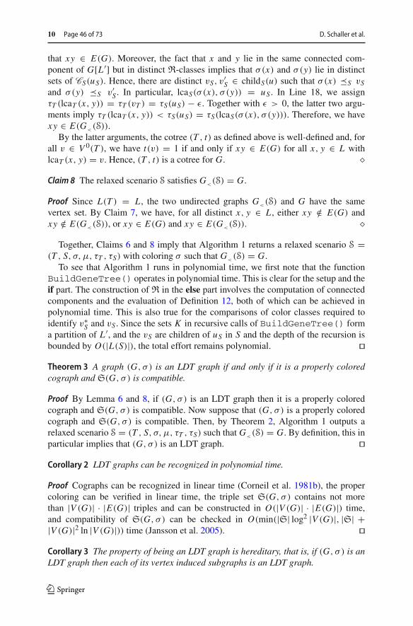
10 Page 46 of 73 D. Schaller et al.
that xy ∈ E(G). Moreover, the fact that x and y lie in the same connected com-ponent of G[L ′] but in distinct R-classes implies that σ(x) and σ(y) lie in distinctsets of CS(uS). Hence, there are distinct vS, v
′S ∈ childS(u) such that σ(x) S vS
and σ(y) S v′S . In particular, lcaS(σ (x), σ (y)) = uS . In Line 18, we assign
τT (lcaT (x, y)) = τT (vT ) = τS(uS) − ε. Together with ε > 0, the latter two argu-ments imply τT (lcaT (x, y)) < τS(uS) = τS(lcaS(σ (x), σ (y))). Therefore, we havexy ∈ E(G<(S)).
By the latter arguments, the cotree (T , t) as defined above is well-defined and, forall v ∈ V 0(T ), we have t(v) = 1 if and only if xy ∈ E(G) for all x, y ∈ L withlcaT (x, y) = v. Hence, (T , t) is a cotree for G. �Claim 8 The relaxed scenario S satisfies G<(S) = G.
Proof Since L(T ) = L , the two undirected graphs G<(S) and G have the samevertex set. By Claim 7, we have, for all distinct x, y ∈ L , either xy /∈ E(G) andxy /∈ E(G<(S)), or xy ∈ E(G) and xy ∈ E(G<(S)). �
Together, Claims 6 and 8 imply that Algorithm 1 returns a relaxed scenario S =(T , S, σ, μ, τT , τS) with coloring σ such that G<(S) = G.
To see that Algorithm 1 runs in polynomial time, we first note that the functionBuildGeneTree() operates in polynomial time. This is clear for the setup and theif part. The construction of R in the else part involves the computation of connectedcomponents and the evaluation of Definition 12, both of which can be achieved inpolynomial time. This is also true for the comparisons of color classes required toidentify v∗
S and vS . Since the sets K in recursive calls of BuildGeneTree() forma partition of L ′, and the vS are children of uS in S and the depth of the recursion isbounded by O(|L(S)|), the total effort remains polynomial. ��Theorem 3 A graph (G, σ ) is an LDT graph if and only if it is a properly coloredcograph and S(G, σ ) is compatible.
Proof By Lemma 6 and 8, if (G, σ ) is an LDT graph then it is a properly coloredcograph and S(G, σ ) is compatible. Now suppose that (G, σ ) is a properly coloredcograph and S(G, σ ) is compatible. Then, by Theorem 2, Algorithm 1 outputs arelaxed scenario S = (T , S, σ, μ, τT , τS) such that G<(S) = G. By definition, this inparticular implies that (G, σ ) is an LDT graph. ��Corollary 2 LDT graphs can be recognized in polynomial time.
Proof Cographs can be recognized in linear time (Corneil et al. 1981b), the propercoloring can be verified in linear time, the triple set S(G, σ ) contains not morethan |V (G)| · |E(G)| triples and can be constructed in O(|V (G)| · |E(G)|) time,and compatibility of S(G, σ ) can be checked in O(min(|S| log2 |V (G)|, |S| +|V (G)|2 ln |V (G)|)) time (Jansson et al. 2005). ��Corollary 3 The property of being an LDT graph is hereditary, that is, if (G, σ ) is anLDT graph then each of its vertex induced subgraphs is an LDT graph.
123

Indirect identification of horizontal gene transfer Page 47 of 73 10
A B C D
Fig. 16 A relaxed scenario S (A) with gene tree T (B) and its associated graph (G<(S), σ ) (C). Thediscriminating cotree TG<(S) (D) is not displayed by T
Proof Let (G = (V , E), σ ) be an LDT graph. It suffices to show that (G− x, σ|V \{x})is an LDT graph, where G − x is obtained from G by removing x ∈ V and all itsincident edges. By Proposition 2, G − x is a cograph that clearly remains properlycolored. Moreover, every induced path on three vertices in G − x is also an inducedpath on three vertices in G. This implies that if xy|z ∈ S′ = S(G − x, σ|V \{x}),then xy|z ∈ S(G, σ ). Hence,S′ ⊆ S(G, σ ). By Theorem 3,S(G, σ ) is compatible.Hence, any tree that displays all triples inS(G, σ ), in particular, displays all triples inS′. Therefore, S′ is compatible. In summary, (G − x, σ|V \{x}) is a properly coloredcograph and S′ is compatible. By Theorem 3 it is an LDT graph. ��
The relaxed scenarios S explaining an LDT graph (G, σ ) are far from being unique.In fact, we can choose from a large set of trees (S, τS) that is determined only by thetriple set S(G, σ ):
Corollary 4 If (G = (L, E), σ ) is an LDT graph with coloring σ : L → M, thenfor all planted trees S on M that display S(G, σ ) there is a relaxed scenario S =(T , S, σ, μ, τT , τS) that contains σ and S and that explains (G, σ ).
Proof If (G, σ ) is an LDT graph, then the species tree S assigned in Line 1 in Algo-rithm 1 is an arbitrary tree on M displaying S(G, σ ). ��Corollary 5 If (G, σ ) is an LDT graph, then there exists a relaxed scenario S =(T , S, σ, μ, τT , τS) explaining (G, σ ) such that T displays the discriminating cotreeTG of G.
Proof Suppose that (G, σ ) is an LDT graph. By Theorem 3, (G, σ )must be a properlycolored cograph and S(G, σ ) is comparable. Hence, Theorem 2 implies that Algo-rithm 1 constructs a relaxed scenario S = (T , S, σ, μ, τT , τS) explaining (G, σ ). Inparticular, the tree T together with labeling t as specified in Claim 7 is a cotree for G.Since the unique discriminating cotree (TG , t) of G is obtained from any other cotreeby contraction of edges in T , the tree T must display TG . ��
Although, Corollary 5 implies that there is always a relaxed scenario S wherethe tree T displays the discriminating cotree TG of G = G(S), this is not true forall relaxed scenarios S with G = G(S). Figure 16 shows a relaxed scenario S′ =(T ′, S′, σ, μ′, τ ′
T , τ ′S) with G = G(S′) for which T ′ does not display TG .
Corollary 5 enables us to relate connectedness of LDT graphs to properties of therelaxed scenarios by which it can be explained.
123

10 Page 48 of 73 D. Schaller et al.
Lemma 11 An LDT graph (G = (L, E), σ ) with |L| > 1 is connected if and onlyif for every relaxed scenario S = (T , S, σ, μ, τT , τS) that explains (G, σ ), we haveτT (ρT ) < τS(lcaS(σ (L))).
Proof By contraposition, suppose first that there is a relaxed scenario S =(T , S, σ, μ, τT , τS) that explains (G, σ ) such that τT (ρT ) ≥ τS(lcaS(σ (L))). Since|L(T )| = |L| > 1, the root ρT is not a leaf. To show that G is disconnected we con-sider two distinct children v,w ∈ child(ρT ) of the root and leaves x ∈ L(T (v)) andy ∈ L(T (w)) and verify that x and y cannot be adjacent in G. If σ(x) = σ(y),then xy /∈ E since (G, σ ) is properly colored (cf. Lemma 8). Hence, supposethat σ(x) �= σ(y). By construction, lcaT (x, y) = ρT and thus, by assumption,τT (lcaT (x, y)) = τT (ρT ) ≥ τS(lcaS(σ (L))). Now lcaS(σ (L)) S lcaS(σ (x), σ (y))implies that τS(lcaS(σ (L))) ≥ τS(lcaS(σ (x), σ (y))) and thus, τT (lcaT (x, y)) ≥τS(lcaS(σ (x), σ (y))). Hence, xy /∈ E . Consequently, for all distinct children v,w ∈child(ρT ), none of the vertices in L(T (v)) are adjacent to any of the vertices inL(T (w)) and thus, G is disconnected.
Conversely, suppose that G is disconnected. We consider Algorithm 1 withinput (G, σ ). By Theorems 2 and 3, the algorithm constructs a relaxed scenarioS = (T , S, σ, μ, τT , τS) that explains (G, σ ). Consider the top-level recursion stepon L and ρS . Since G is disconnected, the vertex uT created in Line 6 of this stepequals the root ρT of the final tree T . To see this, assume first that ρS is a leaf.Then, we attach the |L| > 1 elements in L as leaves to uT (cf. Line 10). Nowassume that ρS is not a leaf. Since G[L] = G has at least two components, weattach at least two vertices vT created in Line 15 to uT . Hence uT is not suppressed inLine 25 and thus ρT = uT . By construction, therefore, we have τT (ρT ) = τT (uT ) =τS(uS) + ε = τS(ρS) + ε for some ε > 0. From σ(ρS) S lcaS(σ (L)) and thedefinition of time maps, we obtain τS(ρS) ≥ τS(lcaS(σ (L))). Therefore, we haveτT (ρT ) ≥ τS(lcaS(σ (L))) + ε > τS(lcaS(σ (L))), which completes the proof. There-fore, we have shown so-far that if all relaxed scenarios S = (T , S, σ, μ, τT , τS) thatexplain (G, σ ) satisfy τT (ρT ) ≤ τS(lcaS(σ (L))), then (G, σ ) must be connected.However, τT (ρT ) = τS(lcaS(σ (L))) cannot occur, since we can reuse the same argu-ments as in the beginning of this proof to show that, in this case, G is disconnected.
��
A.4 Least resolved trees for LDT graphs
As we have seen e.g. in Corollary 4, there are in general many trees S and T formingrelaxed scenarios S that explain a given LDT graph (G, σ ). This begs the question towhat extent these trees are determined by “representatives”. For S, we have seen that Salways displays S(G, σ ), suggesting to consider the role of S = Aho(S(G, σ ), M).This tree is least resolved in the sense that there is no relaxed scenario explaining theLDT graph (G, σ ) with a tree S′ that is obtained from S by edge-contractions. Thelatter is due to the fact that any edge contraction in Aho(S(G, σ ), M) yields a tree S′that does not displayS(G, σ ) any more (Jansson et al. 2012). By Proposition 6, noneof the relaxed scenarios containing S′ explain the LDT (G, σ ).
123
Indirect identification of horizontal gene transfer Page 49 of 73 10
Definition 13 Let S = (T , S, σ, μ, τT , τS) be a relaxed scenario explaining the LDTgraph (G, σ ). The planted tree T is least resolved for (G, σ ) if no relaxed scenario(T ′, S′, σ ′, μ′, τ ′
T , τ ′S) with T ′ < T explain (G, σ ).
In other words, T is least resolved for (G, σ ) if no scenariowith a gene tree T ′ obtainedfrom T by a series of edge contractions explains (G, σ ). The examples in Fig. 3 showthat there is not always a unique least resolved tree.
As outlined in the main part of this paper, the examples in Fig. 3 show that LDTgraphs are in general not accompanied by unique least resolved trees and the examplein Fig. 4 shows that the unique discriminating cotree TG of an LDT graph (G, σ ) isnot always “sufficiently resolved”.
B Horizontal gene transfer and Fitch graphs
B.1 HGT-labeled trees and rs-Fitch graphs
As alluded to in the introduction, the LDT graphs are intimately relatedwith horizontalgene transfer. To formalize this connection we first define transfer edges. These willthen be used to encode Walter Fitch’s concept of xenologous gene pairs (Fitch 2000;Darby et al. 2017) as a binary relation, and thus, the edge set of a graph.
Definition 14 Let S = (T , S, σ, μ, τT , τS) be a relaxed scenario. An edge (u, v) in Tis a transfer edge if μ(u) and μ(v) are incomparable in S. The HGT-labeling of T inS is the edge labeling λS : E(T ) → {0, 1} with λ(e) = 1 if and only if e is a transferedge.
The vertex u in T thus corresponds to an HGT event, with v denoting the subsequentevent, which now takes place in the “recipient” branch of the species tree. Note thatλS is completely determined by S. In general, for a given a gene tree T , HGT eventscorrespond to a labeling or coloring of the edges of T .
Definition 15 (Fitch graph) Let (T , λ) be a tree T together with a map λ : E(T ) →{0, 1}. The Fitch graph �(T , λ) = (V , E) has vertex set V := L(T ) and edge set
E := {xy | x, y ∈ L, the unique path connecting x
and y in T contains an edge e with λ(e) = 1.}
By definition, Fitch graphs of 0/1-edge-labeled trees are loop-less and undirected. Wecall edges e of (T , λ) with label λ(e) = 1 also 1-edges and, otherwise, 0-edges.
Remark 4 Fitch graphs as defined here have been termed undirected Fitch graphs(Hellmuth et al. 2018), in contrast to the notion of the directed Fitch graphs of 0/1-edge-labeled trees studied e.g. inGeiß et al. (2018) andHellmuth and Seemann (2019).
Proposition 5 (Hellmuth et al. 2018; Zverovich 1999) The following statements areequivalent.
1. G is the Fitch graph of a 0/1-edge-labeled tree.
123

10 Page 50 of 73 D. Schaller et al.
2. G is a complete multipartite graph.3. G does not contain K2 + K1 as an induced subgraph.
A natural connection between LDT graphs and complete multipartite graphs issuggested by the definition of triple setsT(G), since each forbidden induced subgraphK2 + K1 of a complete multipartite graphs corresponds to a triple in an LDT graph.More precisely, we have:
Lemma 12 (G, σ ) is a properly colored complete multipartite if and only if it is prop-erly colored and T(G) = ∅.Proof The equivalence between the statements can be seen by observing that G is acomplete multipartite graph if and only if G does not contain an induced K2 + K1 (cf.Proposition 5). By definition of T(G), this is the case if and only if T(G) = ∅. ��Definition 16 (rs-Fitch graph) Let S = (T , S, σ, μ, τT , τS) be a relaxed scenario withHGT-labeling λS. We call the vertex colored graph (�(S), σ ) := (�(T , λS), σ ) theFitch graph of the scenario S.A vertex colored graph (G, σ ) is a relaxed scenario Fitch graph (rs-Fitch graph) ifthere is a relaxed scenario S = (T , S, σ, μ, τT , τS) such that G = �(S).
Figure 5 shows that rs-Fitch graphs are not necessarily properly colored. A subtledifficulty arises from the fact that Fitch graphs of 0/1-edge-labeled trees are definedwithout a reference to the vertex coloring σ , while the rs-Fitch graph is vertex colored.
Observation 1 If (G, σ ) is an rs-Fitch graph then G is a complete multipartite graph.
The “converse” of Observation 1 is not true in general, as we shall see in Theorem 6below. If, however, the coloring σ can be chosen arbitrarily, then every complete mul-tipartite graphG can be turned into an rs-Fitch graph (G, σ ) as shown in Proposition 6.
Proposition 6 If G is a complete multipartite graph, then there exists a relaxed sce-nario S = (T , S, σ, μ, τT , τS) such that (G, σ ) is an rs-Fitch graph.
Proof Let G be a complete multipartite graph and set L := V (G) and R := E(G).If R = ∅, then the relaxed scenario S constructed in the proof of Lemma 4 showsthat E(G) = E(�(S)) = ∅. Hence, we assume that R �= ∅ and explicitly construct arelaxed scenario S = (T , S, σ, μ, τT , τS) such that (G, σ ) is an rs-Fitch graph.
We start by specifying the coloring σ : L → M . Since G is a complete multipartitegraph it is determined by its independent sets I1, . . . , Ik , which form a partition of L .We set M := {1, 2, . . . , k} and color every x ∈ I j with color σ(x) = j , 1 ≤ j ≤ k.By construction, (G, σ ) is properly colored, and σ(x) = σ(y) whenever xy /∈ R, i.e.,whenever x and y lie in the same independent set. Therefore, we have S(G, σ ) = ∅.Let S be the planted star tree with leaf set L(S) = {1, . . . , k} = M and childS(ρS) =M . Since R �= ∅, we have k ≥ 2, and thus, ρS has at least two children and is, therefore,phylogenetic. We choose the time map τS by putting τS(0S) = 2, τS(ρS) = 1 andτS(x) = 0 for all x ∈ L(S).
123

Indirect identification of horizontal gene transfer Page 51 of 73 10
Fig. 17 Construction in the proof of Proposition 6
Finally, we construct the planted phylogenetic tree T with planted root 0T and rootρT as follows: Vertex ρT has k children u1, . . . , uk . If I j = {x j } consists of a singleelement, then we put u j := x j as a leaf or T , and otherwise, vertex u j has exactly |I j |children where child(u j ) = I j . Now label, for all i ∈ {2, . . . , k}, the edge (ρT , ui )with “1”, and all other edges with “0”. Since k ≥ 2, the tree T is also phylogenetic byconstruction.
We specify the time map τT and the reconciliation map μ by defining, for everyv ∈ V (T ),
τT (v) :=
⎧⎪⎪⎪⎨
⎪⎪⎪⎩
2 = τS(0S)
0
1/2
1/4
μ(v) :=
⎧⎪⎪⎪⎨
⎪⎪⎪⎩
0S if v = 0T ,
σ (v) if v ∈ L(T ),
(ρS, 1) if v = ρT , and
(ρS, i) if v = ui /∈ L(T ), 1 ≤ i ≤ k.
With the help of Fig. 17, it is now easy to verify that (i) τT is a time map for T ,(ii) the reconciliation map μ is time-consistent, and (iii) λS = λ. In summary, S =(T , S, σ, μ, τT , τS) is a relaxed scenario, and (G, σ ) = (�(S), σ ) is an rs-Fitch graph.
��
Although every complete multipartite graph can be colored in such a way that itbecomes an rs-Fitch graph (cf. Proposition 6), there are colored, complete multipartitegraphs (G, σ ) that are not rs-Fitch graphs, i.e., that do not derive from a relaxedscenario (cf. Theorem 6). We summarize this discussion in the following
Observation 2 There are (planted) 0/1-edge labeled trees (T , λ) and coloringsσ : L(T ) → M such that there is no relaxed scenario S = (T , S, σ, μ, τT , τS) withλ = λS.
A subtle—but important—observation is that trees (T , λ) with coloring σ for whichObservation 2 applies may still encode an rs-Fitch graph (�(T , λ), σ ), see Example 1and Fig. 6. The latter is due to the fact that �(T , λ) = �(T ′, λ′) may be possible for adifferent tree (T ′, λ′) for which there is a relaxed scenario S′ = (T ′, S, σ, μ, τT , τS)
with λ′ = λS. In this case, (�(T , λ), σ ) = (�(S′), σ ) is an rs-Fitch graph. We shallbriefly return to these issues in the discussion Sect. 8.
123

10 Page 52 of 73 D. Schaller et al.
B.2 LDT graphs and rs-Fitch graphs
We proceed to investigate to what extent an LDT graph provides information aboutan rs-Fitch graph. As we shall see in Theorem 5 there is indeed a close connectionbetween rs-Fitch graphs and LDT graphs. We start with a useful relation between theedges of rs-Fitch graphs and the reconciliation maps μ of their scenarios.
Lemma 13 Let �(S) be an rs-Fitch graph for some relaxed scenario S. Then, ab /∈E(�(S)) implies that lcaS(σ (a), σ (b)) S μ(lcaT (a, b)).
Proof Assume first that ab /∈ E(�(S)) and denote by Pxy the unique path in T thatconnects the two vertices x and y. Clearly, u := lcaT (a, b) is contained in Pab, andthis path Pab can be subdivided into the two paths Pu,a and Pu,b that have only vertexu in common. Since ab /∈ E(�(S)), none of the edges (v,w) along the path Pab in T isa transfer edge, and thus, the imagesμ(v) andμ(w) are comparable in S. This impliesthat the images of any two vertices along the path Pu,a as well as the images of anytwo vertices along Pu,b are comparable. In particular, therefore, μ(u) is comparablewith both μ(a) = σ(a) =: A and μ(b) = σ(b) =: B, where we may have A = B.Together with the fact that A and B are leaves in S, this implies thatμ(u) is an ancestorof A and B. Since lcaS(A, B) is the “last” vertex that is an ancestor of both A and B,we have lcaS(A, B) S μ(u). ��
The next result shows that a subset of transfer edges can be inferred immediatelyfrom LDT graphs:
Theorem 4 If (G, σ ) is an LDT graph, then G ⊆ �(S) for all relaxed scenarios Sthat explain (G, σ ).
Proof Let S = (T , S, σ, μ, τT , τS) be a relaxed scenario that explains (G, σ ), i.e.,G = G<(S). By definition, V (G) = V (�(S)) = L(T ). Hence it remains to show thatE(G) ⊆ E(�(S)). To this end, consider ab ∈ E(G) and assume, for contradiction,that ab /∈ E(�(S)). Let A := σ(a) and B := σ(b). By Lemma 13, lcaS(A, B) S
μ(lcaT (a, b)). But then, by Definitions 3 and 4, τS(lcaS(A, B)) ≤ τS(lcaT (a, b)),implying ab /∈ E(G), a contradiction. ��
Since we only have that xy is an edge in �(S) if the path connecting x and y in thetree T of S contains a transfer edge, Theorem 4 immediately implies
Corollary 6 For every relaxed scenario S = (T , S, σ, μ, τT , τS) without transferedges, it holds that E(G<(S)) = ∅.
Theorem 4 provides the formal justification for indirect phylogenetic approachesto HGT inference that are based on the work of Lawrence and Hartl (1992), Clarkeet al. (2002), and Novichkov et al. (2004) by showing that xy ∈ E(G<(S)) can beexplained only byHGT, irrespective of how complex the true biological scenariomighthave been. However, it does not cover all HGT events. Figure 7 shows that there arerelaxed scenarios S for which G<(S) �= �(S) even though �(S) is properly colored.Moreover, it is possible that an rs-Fitch graph (G, σ ) contains edges xy ∈ E(G) withσ(x) = σ(y). In particular, therefore, an rs-Fitch graph is not always an LDT graph.
123

Indirect identification of horizontal gene transfer Page 53 of 73 10
It is natural, therefore, to ask whether for every properly colored Fitch graph thereis a relaxed scenario S such that G<(S) = �(S). An affirmative answer is providedby
Theorem 5 The following statements are equivalent.
1. (G, σ ) is a properly colored complete multipartite graph.2. There is a relaxed scenario S = (T , S, σ, μ, τT , τS) with coloring σ such that
G = G<(S) = �(S).3. (G, σ ) is complete multipartite and an LDT graph.4. (G, σ ) is properly colored and an rs-Fitch graph.
In particular, for every properly colored complete multipartite graph (G, σ ) the tripleset S(G, σ ) is compatible.
Proof (1) implies (2). We assume that (G, σ ) is a properly colored multipartite graphand set L := V (G) and E := E(G). If E = ∅, then the relaxed scenario S con-structed in the proof of Lemma 4 satisfies G = G<(S) = �(S), i.e., the graphs areedgeless. Hence, we assume that E �= ∅ and explicitly construct a relaxed scenarioS = (T , S, σ, μ, τT , τS) with coloring σ such that G = G<(S) = �(S).
The graph (G, σ ) is properly colored and complete multipartite by assumption. LetI1, . . . , Ik denote the independent sets of G. Since E �= ∅, we have k > 1. Since allx ∈ Ii are adjacent to all y ∈ I j , i �= j and (G, σ ) is properly colored, it must hold
that σ(Ii ) ∩ σ(I j ) = ∅. For a fixed i let v1i , . . . v|Ii |i denote the elements in Ii .
We first start with the construction of the species tree S. First we add a planted root0S with child ρS . Vertex ρS has children w1, . . . , wk where each w j corresponds toone I j . Note, σ : L → M may not be surjective, in which case we would add oneadditional child x to ρS for each color x ∈ M\σ(L).
If |σ(I j )| = 1, then we identify the single color x ∈ σ(I j ) with w j . Otherwise,i.e., if |σ(I j )| > 1, vertex w j has as children the set childS(w j ) = σ(I j ) which areleaves in S. See Fig. 18 for an illustrative example. Now we can choose the time mapτS for S such τS(0S) = 3, τS(ρS) = 2, τS(x) = 0 for all x ∈ L(S) and τS(x) = 1 forall x ∈ V 0(S)\{ρS}.
We now construct T as follows. The tree T has planted root 0T with child ρT .Vertex ρT has k children u1, . . . , uk where each u j corresponds to one I j . Vertex u j isa leaf if |I j | = 1, and, otherwise, has exactly |I j | children that are uniquely identifiedwith the elements in I j .
We now define the time map τT and reconciliation map μ for v ∈ V (T ):
τT (v) :=
⎧⎪⎪⎪⎨
⎪⎪⎪⎩
3 = τS(0S)
0
1.5
1.25
μ(v) :=
⎧⎪⎪⎪⎨
⎪⎪⎪⎩
0S if v = 0T ,
σ (v) if v ∈ L(T ),
(ρS, w1) if v = ρT , and
(ρS, wi ) if v = ui /∈ L(T ), 1 ≤ i ≤ k.
With the help of Fig. 18 it is now easy to verify that (i) τT is a time map for T ,and that (ii) the reconciliation map μ is time-consistent. In summary the constructedS = (T , S, σ, μ, τT , τS) is a relaxed scenario.
123
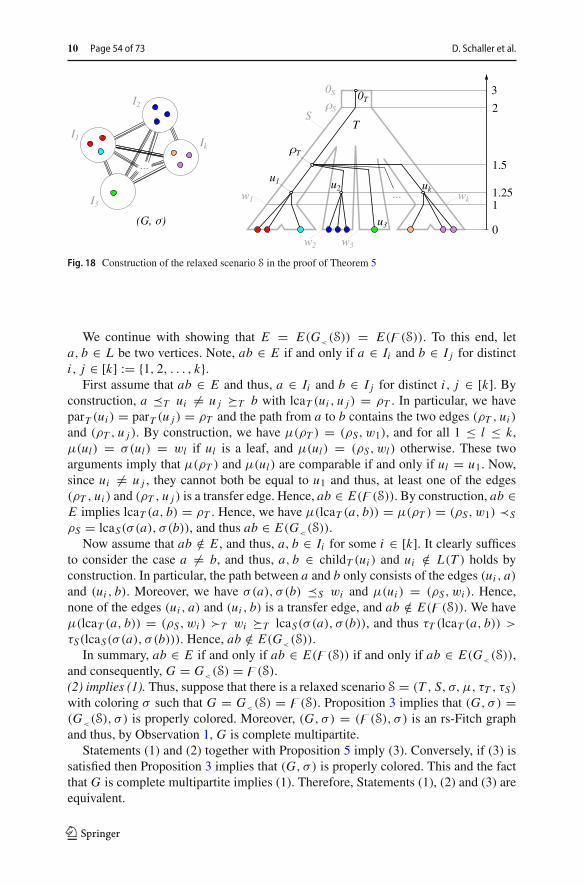
10 Page 54 of 73 D. Schaller et al.
Fig. 18 Construction of the relaxed scenario S in the proof of Theorem 5
We continue with showing that E = E(G<(S)) = E(�(S)). To this end, leta, b ∈ L be two vertices. Note, ab ∈ E if and only if a ∈ Ii and b ∈ I j for distincti, j ∈ [k] := {1, 2, . . . , k}.
First assume that ab ∈ E and thus, a ∈ Ii and b ∈ I j for distinct i, j ∈ [k]. Byconstruction, a T ui �= u j T b with lcaT (ui , u j ) = ρT . In particular, we haveparT (ui ) = parT (u j ) = ρT and the path from a to b contains the two edges (ρT , ui )and (ρT , u j ). By construction, we have μ(ρT ) = (ρS, w1), and for all 1 ≤ l ≤ k,μ(ul) = σ(ul) = wl if ul is a leaf, and μ(ul) = (ρS, wl) otherwise. These twoarguments imply that μ(ρT ) and μ(ul) are comparable if and only if ul = u1. Now,since ui �= u j , they cannot both be equal to u1 and thus, at least one of the edges(ρT , ui ) and (ρT , u j ) is a transfer edge. Hence, ab ∈ E(�(S)). By construction, ab ∈E implies lcaT (a, b) = ρT . Hence, we have μ(lcaT (a, b)) = μ(ρT ) = (ρS, w1) ≺S
ρS = lcaS(σ (a), σ (b)), and thus ab ∈ E(G<(S)).Now assume that ab /∈ E , and thus, a, b ∈ Ii for some i ∈ [k]. It clearly suffices
to consider the case a �= b, and thus, a, b ∈ childT (ui ) and ui /∈ L(T ) holds byconstruction. In particular, the path between a and b only consists of the edges (ui , a)
and (ui , b). Moreover, we have σ(a), σ (b) S wi and μ(ui ) = (ρS, wi ). Hence,none of the edges (ui , a) and (ui , b) is a transfer edge, and ab /∈ E(�(S)). We haveμ(lcaT (a, b)) = (ρS, wi ) �T wi T lcaS(σ (a), σ (b)), and thus τT (lcaT (a, b)) >
τS(lcaS(σ (a), σ (b))). Hence, ab /∈ E(G<(S)).In summary, ab ∈ E if and only if ab ∈ E(�(S)) if and only if ab ∈ E(G<(S)),
and consequently, G = G<(S) = �(S).(2) implies (1). Thus, suppose that there is a relaxed scenario S = (T , S, σ, μ, τT , τS)
with coloring σ such that G = G<(S) = �(S). Proposition 3 implies that (G, σ ) =(G<(S), σ ) is properly colored. Moreover, (G, σ ) = (�(S), σ ) is an rs-Fitch graphand thus, by Observation 1, G is complete multipartite.
Statements (1) and (2) together with Proposition 5 imply (3). Conversely, if (3) issatisfied then Proposition 3 implies that (G, σ ) is properly colored. This and the factthat G is complete multipartite implies (1). Therefore, Statements (1), (2) and (3) areequivalent.
123

Indirect identification of horizontal gene transfer Page 55 of 73 10
Furthermore, (4) implies (1) by Observation 1. Conversely, (G, σ ) in Statement (2)is an rs-Fitch graph and an LDT graph. Hence it is properly colored by Proposition 3.Thus (2) implies (4).
Statement (3), in particular, implies that every properly colored complete multi-partite (G, σ ) is an LDT graph and, thus, there is a relaxed scenario S such thatG = G<(S). Now, we can apply Lemma 6 to conclude that S(G, σ ) is compatible,which completes the proof. ��Corollary 7 A colored graph (G, σ ) is an LDT graph and an rs-Fitch graph if andonly if (G, σ ) is a properly colored complete multipartite graph (and thus, a properlycolored Fitch graph for some 0/1-edge-labeled tree).
Proof If (G, σ ) is an rs-Fitch graph then, by Observation 1, G is a complete multi-partite graph. Moreover, since (G, σ ) is an LDT graph, (G, σ ) is properly colored(cf. Proposition 3). Conversely, if (G, σ ) is a properly colored complete multipartitegraph it is, by Theorem 5(2), an rs-Fitch graph and an LDT graph. Now the equivalencebetween Statements (1) and (3) in Theorem 5 shows that (G, σ ) is an LDT graph. ��Corollary 8 Let (G, σ ) be a vertex-colored graph. IfT(G) = ∅ andS(G, σ ) is incom-patible, then G is a complete multipartite graph (and thus, a Fitch graph for some0/1-edge-labeled tree), but σ is not a proper vertex coloring of G.
Proof By definition, if T(G) = ∅, then G cannot contain an induced K2 + K1. ByProposition 5, G is a Fitch graph. Contraposition of the last statement in Theorem 5andG being a Fitch graph for some (T , λ) implies that σ is not a proper vertex coloringof G. ��
As outlined in the main part of this paper, LDT graphs are sufficient to describereplacing HGT. They fail, however, to describe additive HGT in full detail.
B.3 rs-Fitch graphs with general colorings
In scenarios with additive HGT, the rs-Fitch graph is no longer properly colored andno-longer coincides with the LDT graph. Since not every vertex-colored completemultipartite graphs (G, σ ) is an rs-Fitch graph (cf. Theorem 6), we ask whether anLDT graph (G, σ ) that is not itself already an rs-Fitch graph imposes constraintson the rs-Fitch graphs (�(S), σ ) that derive from relaxed scenarios S that explain(G, σ ). As a first step towards this goal, we aim to characterize rs-Fitch graphs, i.e.,to understand the conditions imposed by the existence of an underlying scenario S onthe compatibility of the collection of independent setsI of G and the coloring σ . Aswe shall see, these conditions can be explained in terms of an auxiliary graph that weintroduce in a very general setting:
Definition 17 Let L be a set, σ : L → M a map andI = {I1, . . . , Ik} a set of subsetsof L . Then the graph A�(σ,I ) has vertex set M and edges xy if and only if x �= yand x, y ∈ σ(I ′) for some I ′ ∈ I . We define an edge labeling � : E(A�) → 2I
such that �(e) := {I ∈ I | ∃x, y ∈ I s.t. σ(x)σ (y) = e}.
123

10 Page 56 of 73 D. Schaller et al.
By construction A�(σ,I ′) is a subgraph of A�(σ,I ) whenever I ′ ⊆ I . Thelabeling of an edge e records the sets I ∈ I that imply the presence of the edge.
Theorem 6 Agraph (G, σ ) is an rs-Fitch graph if and only if (i) it is completemultipar-tite with independent setsI = {I1, . . . , Ik}, and (ii) if k > 1, there is an independentset I ′ ∈ I such that A�(σ,I \{I ′}) is disconnected.
Proof Let G = (L, E) be a graph with coloring σ : L → M . Suppose first that Gsatisfies (i) and (ii). To show that (G, σ ) is an rs-Fitch graph,wewill construct a relaxedscenario S = (T , S, σ, μ, τT , τS) such that G = �(S). If k = 1, or equivalentlyE = ∅, then the relaxed scenario S constructed in the proof of Lemma 4 satisfiesG = �(S), i.e., both graphs are edgeless. Now assume that k > 1 and thus, E �= ∅.Hence, we can choose an independent set I ′ ∈ I such that A′
�:= A�(σ,I \{I ′})
is disconnected. Note that I \{I ′} is non-empty since k > 1. Moreover, since A′�is
a disconnected graph on the color set M , there is a connected component C of A′�
such that (M\C) ∩ σ(I ′) �= ∅. Hence M1 := M\C and M2 := C form a bipartitionof M such that neither M1 nor M2 are empty sets.
We continue by showing that every I ∈ I \{I ′} satisfies either σ(I ) ⊆ M1 orσ(I ) ⊆ M2. To see this, assume, for contradiction, that there are colors A ∈ σ(I )∩M1and B ∈ σ(I ) ∩ M2 for some I ∈ I \{I ′}. Thus, B ∈ C and, by definition, AB ∈E(A′
�). Therefore, A and B must lie in the connected component C ; a contradiction.
Therefore, we can partition I \{I ′} into I1 := {I ∈ I \{I ′} | σ(I ) ⊆ M1} andI2 := {I ∈ I \{I ′} | σ(I ) ⊆ M2}. Note that one of the setsI1 andI2, but not bothof them, may be empty. This may be the case, for instance, if σ is not surjective.
Now, we construct a relaxed scenario S = (T , S, σ, μ, τT , τS) with coloring σ
such that G = �(S). We first define the species tree S as the planted tree where ρS
(i.e. the single child of 0S) hast two children w1 and w2. If |M1| = 1, we identify w1with the single element in M1, and otherwise, we set childS(w1) = L(S(w1)) := M1.We proceed analogously for w2 and M2. Thus, S is phylogenetic by construction. Wechoose the time map τS by putting τS(0S) = 2, τS(ρS) = 1, τS(w1) = τS(w2) = 0.5and τS(x) = 0 for all x ∈ L(S). This completes the construction of S and τS .
We proceed with the construction of the gene tree T , its time map τT and thereconciliation map μ. This tree T has leaf set L , planted root 0T , and root ρT . We setμ(0T ) = 0S and τT (0T ) = τS(0S) = 2, and moreover μ(x) = σ(x) and τT (x) = 0for all x ∈ L .
For each I j ∈ I \{I ′}, we add a vertex u j . We will later specify how these verticesare connected (via paths) to ρT . If |I j | = 1, u j becomes a leaf of T that is identifiedwith the unique element in I j . Otherwise, we add exactly |I j | children to u j , each ofwhich is identified with one of the elements in I j . If u j is a leaf, we already definedμ(u j ) = σ(u j ) and τT (u j ) = 0.
Otherwise, we set τT (u j ) = 0.6 and μ(u j ) = (ρS, w1) if I j ∈ I1 and μ(u j ) =(ρS, w2) if I j ∈ I2. Recall that M1 ∩ σ(I ′) �= ∅. However, both M2 ∩ σ(I ′) �= ∅and M2 ∩ σ(I ′) = ∅ are possible. The latter case appears e.g. whenever A�(σ,I )
was already disconnected. To connect the vertices u j to ρT , we distinguish the threemutually exclusive cases:Case (a): M2 ∩ σ(I ′) = ∅ and I1 �= ∅.
123

Indirect identification of horizontal gene transfer Page 57 of 73 10
A B C
Fig. 19 Illustration of the relaxed scenario constructed in the if -direction of the proof of Theorem 6. ForCases (a) and (c), only the situation in which a vertex u′ and u′′, resp., is necessary is shown. Otherwise,the single element in I ′, I ′1 or I ′2 would be a child of the root ρT . Moreover, the vertices u j are drawn underthe assumption that |I j | > 1. Otherwise, there are identified with the single leaf in I j
We set μ(ρT ) = (ρS, w2) and τT (ρT ) = 0.9. We attach all u j that correspond toelements I j ∈ I1 as children of ρT . If |I ′| > 1 or I2 �= ∅, we create a vertex u′ towhich all elements in I ′ and all u j such that I j ∈ I2 are attached as children, attach u′as a child of ρT , and set μ(u′) = (ρS, w1) and τT (u′) = 0.75. Otherwise, we simplyattach the single element x ′ in I ′ as a child of ρT . Clearly, the so constructed tree T isphylogenetic. Note that the edges (ρT , u j ) with I j ∈ I1 as well as the edges (u′, u j )
with I j ∈ I2 are transfer edges. Together with (ρT , u′) or (ρT , x), respectively, theseare the only transfer edges.Case (b): M2 ∩ σ(I ′) = ∅ and I1 = ∅.By the arguments above, the latter implies I2 �= ∅. Hence, we can set μ(ρT ) =(ρS, w1) and τT (ρT ) = 0.9 and attach all elements of I ′ as well as the vertices u j
corresponding to the independent sets I j ∈ I2 = I \{I ′} as children of ρT . Since|I ′| ≥ 1 and I2 ≥ 1, the tree T obtained in this manner is again phylogenetic.Moreover, note that the transfer edges are exactly the edges (ρT , u j ).Case (c): M2 ∩ σ(I ′) �= ∅.In this case, the sets I ′
1 := {x ∈ I ′ | σ(x) ∈ M1} and I ′2 := {x ∈ I ′ | σ(x) ∈ M2}
must be non-empty. We set μ(ρT ) = (0T , ρT ) and τT (ρT ) = 1.5. If |I ′1| > 1 or
I2 �= ∅, we create a vertex u′ to which all elements in I ′1 and all u j such that I j ∈ I2
are attached as children, and set μ(u′) = (ρS, w1) and τT (u′) = 0.75. Otherwise, wesimply attach the single element in I ′
1 as a child of ρT . For the “other side”, we proceedanalogously: If |I ′
2| > 1 or I1 �= ∅, we create a vertex u′′ to which all elements in I ′2
and all u j such that I j ∈ I1 are attached as children, and set μ(u′) = (ρS, w2) andτT (u′′) = 0.75. Otherwise, we simply attach the single element in I ′
2 as a child of ρT .By construction, the so constructed tree is again phylogenetic. Moreover, the transferedges are exactly the edges (u′, u j ) and (u′′, u j ).
Using Fig. 19, one can easily verify that, in all three Cases (a)-(c), the reconciliationmap μ is time-consistent with τT and τS . Thus, S is a relaxed scenario. Moreover,Fig. 19 together with the fact that σ(I ) ⊆ M1 holds for all I ∈ I1, and σ(I ) ⊆ M2holds for all I ∈ I2, shows that G = �(S) in all three cases. Hence, (G, σ ) is anrs-Fitch graph.
123

10 Page 58 of 73 D. Schaller et al.
For the only-if -direction, assume that (G = (V , E), σ ) is an rs-Fitch graph. Hence,there exists a relaxed scenarioS = (T , S, σ, μ, τT , τS) such thatG = �(S). ByObser-vation 1 and Proposition 5, (G, σ ) is a complete multipartite graph that is determinedby its set of independent sets I = {I1, . . . , Ik}. Hence, Condition (i) is satisfied.
Now assume, for contradiction, that Condition (ii) is violated. Thus k ≥ 2 and thereis no independent set I ′ ∈ C such that A�(σ,I \{I ′}) is disconnected. If |M | = 1,then the species tree S only consists of the planted root 0S and the root ρS , whichin this case is identified with the single element in M . Clearly, all vertices and edgesare comparable in such a tree S, and hence, there is no transfer edges in S, implyingE = ∅ and thus |I | = 1; a contradiction to k ≥ 2.
Thus we have |M | ≥ 2 and the root ρS of the species tree S has at least twochildren. Since A�(σ,I \{I ′}) is connected for every I ′ ∈ C , the graph A�(σ,I )
is also connected. Since each color appears at most once as a leaf of S, σ(L(S(v1)))∩σ(L(S(v2))) = ∅ holds for any two distinct children v1, v2 ∈ childS(ρS). These threeassertions, together with the definition of the auxiliary graph A�(σ,I ), imply thatthere are two distinct colors A, B ∈ M such that AB is an edge inA�(σ,I ), A S v1and B ≺S v2 for distinct children v1, v2 ∈ childS(ρS). By definition of A�(σ,I )
there is an independent set I ′ ∈ I containing a vertex a ∈ I ′ with σ(a) = A and avertex b ∈ I ′ with σ(b) = B. Since a and b lie in the same independent set, we haveab /∈ E . By Lemma 13, μ(lcaT (a, b)) S lcaS(A, B) = ρS . Since, by assumption,A�(σ,I \{I ′}) is also connected, we find two distinct colorsC and D (not necessarilydistinct from A and B) such that CD is an edge in A�(σ,I ), C S v3 and D ≺S v4for distinct children v3, v4 ∈ childS(ρS) (but not necessarily distinct from v1 and v2),and in particular, an independent set I ′′ ∈ I \{I ′} containing a vertex c ∈ I ′′ withσ(c) = C and a vertex d ∈ I ′′ with σ(d) = D. By construction, I ′ �= I ′′, and thus,all edges between I ′ and I ′′ exist in G, in particular the edges ac, ad, bc, bd. Sincec, d ∈ I ′′, we have cd /∈ E and thus, by Lemma 13, μ(lcaT (c, d)) S lcaS(C, D) =ρS .
We now consider the unique path P in T that connects lcaT (a, b) and lcaT (c, d).Sinceμ is time-consistent andμ(lcaT (a, b)), μ(lcaT (c, d)) S ρS , we conclude that,for every edge uv along this path P , we haveμ(u), μ(v) S ρS and thusμ(u), μ(v) ∈{ρS, (0S, ρS)}. But then, μ(u) and μ(v) are comparable in S. Therefore, P does notcontain any transfer edge. Since ab /∈ E , the path connecting a and lcaT (a, b) doesnot contain any transfer edges. Likewise, cd /∈ E implies that the path connecting cand lcaT (c, d) does not contain any transfer edges. Thus, the path connecting a andc also does not contain any transfer edge, which implies that ac /∈ E(�(S)) = E ; acontradiction since a and c belong to two distinct independent sets.
Hence, we conclude that for k > 1 there exists an independent set I ′ ∈ C such thatA�(σ,I \{I ′}) is disconnected. ��Corollary 9 rs-Fitch graphs can be recognized in polynomial time.
Proof Every rs-Fitch graph (G, σ ) must be complete multipartite, which can be veri-fied in polynomial time. In this case, the set of independent sets I = {I1, . . . , Ik} ofG can also be determined and the graph A�(σ,I ) can be constructed in polynomialtime. Finally, we need to find an independent set I ′ ∈ I , such thatA�(σ,I \{I ′}) isdisconnected. Clearly, checking whetherA�(σ,I \{I ′}) is disconnected can be done
123
Indirect identification of horizontal gene transfer Page 59 of 73 10
in polynomial time and since there are at most |V (G)| independent sets inI , findingan independent set I ′ such that A�(σ,I \{I ′}) is disconnected (if one exists) can bedone in polynomial time as well. ��Corollary 10 Let (G, σ ) be a complete multipartite graph with coloring σ : V (G) →M and set of independent sets I . Then, (G, σ ) is an rs-Fitch graph if and only ifA�(σ,I ) is disconnected or there is a cut Q ⊆ E(A�(σ,I )) such that all edgese ∈ Q have the same label �(e) = {I } for some I ∈ I .
Proof IfA�(σ,I ) is disconnected, thenA�(σ,I \{I }) remains disconnected for allI ∈ I and, by Theorem 6, (G, σ ) is an rs-Fitch graph.
If there is a cut Q ⊆ E(A�(σ,I )) such that all edges e ∈ Q have the samelabel �(e) = {I } for some I ∈ I , then, by definition, E(A�(σ,I \{I })) ⊆ E ′ :=E(A�(σ,I ))\Q. Since Q is a cut in A�(σ,I ), the resulting graph A′
�= (M, E ′)
is disconnected. By the latter arguments, A�(σ,I \{I }) is a subgraph of A′�, and
thus, disconnected as well. By Theorem 6, (G, σ ) is an rs-Fitch graph.Conversely, if (G, σ ) is an rs-Fitchgraph, thenTheorem6 implies thatA�(σ,I \{I })
is disconnected for some I ∈ I . If A�(σ,I ) was already disconnected, then thereis nothing to show. Hence assume that A�(σ,I ) = (M, E) is connected and letA�(σ,I \{I }) = (M, E ′). Moreover, let F ⊆ E be the subset of edges e ∈ Ewith I ∈ �(e). Note, F contains all edges of E that have potentially been removedfrom E to obtain E ′. However, all edges e = xy in F with |�(e)| > 1 must remainin A�(σ,I \{I }), since there is another independent set I ′ ∈ �(e)\{I } such thatx, y ∈ σ(I ′). Hence, only those edges e in F for which |�(e)| = 1 are removed fromE . Hence, there is a cut Q ⊆ F ⊆ E such that all edges e ∈ Q have the same label�(e) = {I } for some I ∈ I . ��Corollary 11 If (G, σ ) with coloring σ : V (G) → M is an rs-Fitch graph, then thereare no two disjoint independent sets I and I ′ of G with σ(I ) = σ(I ′) = M.
Proof Let I be the set of independent sets of G. If |I | = 1, there is nothing toshow and thus, we assume that |I | > 1. Assume, for contradiction, that there aretwo distinct independent sets I , I ′ ∈ I such that σ(I ) = σ(I ′) = M . For everyI ′′ ∈ I , the set I \{I ′′} clearly contains at least one of the two sets I and I ′, both ofwhich contain all colors in M . Therefore, A�(σ,I \{I ′′}) is the complete graph byconstruction and, thus, connected for every I ′′ ∈ I . This together with Theorem 6implies that (G, σ ) is not an rs-Fitch graph; a contradiction. ��Corollary 12 Every complete multipartite graph (G, σ ) with a vertex coloringσ : V (G) → M that is not surjective is an rs-Fitch graph.
Proof If σ : V (G) → M is not surjective, then A�(σ,I ) is disconnected, where Idenotes the set of independent sets ofG. Hence, if k > 1, thenA�(σ,I \{I }) remainsdisconnected for all I ∈ I . By Theorem 6, (G, σ ) is an rs-Fitch graph. ��
Corollary 12 may seem surprising since it implies that the property of being anrs-Fitch graph can depend on species (colors M) for which we have no genes L inthe data. The reason is that an additional lineage in the species tree provides a place
123

10 Page 60 of 73 D. Schaller et al.
to “park” interior vertices in the gene tree from which HGT-edges can emanate thatcould not always be accommodated within lineages that have survivors—where theymay force additional HGT edges.
Corollary 13 Every Fitch graph (G, σ ) that contains an independent set I and a vertexx ∈ I with σ(x) /∈ σ(I ′) for all other independent sets I ′ �= I , is an rs-Fitch graph.
Proof Let I denote the set of independent sets of G. If there is an independent setI ∈ I that contains a vertex x ∈ I with σ(x) /∈ σ(I ′) for all other independentsets I ′ �= I , then the vertex σ(x) in A�(σ,I \{I }) is an isolated vertex and thus,A�(σ,I \{I }) is disconnected. By Theorem 6, (G, σ ) is an rs-Fitch graph. ��As for LDT graphs, the property of being an rs-Fitch graph is hereditary.
Corollary 14 If (G = (L, E), σ ) is an rs-Fitch graph, then the colored vertex inducedsubgraph (G[W ], σ|W ) is an rs-Fitch graph for all non-empty subsets W ⊆ L.
Proof It suffices to show the statement for W = L\{x} for an arbitrary vertex x ∈ L .If G = (L, E) is edgeless, then G[W ] is edgeless and thus, by Theorem 6, an rs-Fitchgraph.
Thus, assume that E �= ∅ and thus, for the set I of independent sets of G it holdsthat |I | > 1. Since G does not contain an induced K2 + K1, it is easy to see thatG[W ] cannot contain an induced K2 + K1 and thus, G[W ] is a complete multipartitegraph. Hence, Theorem 6(i) is satisfied. Moreover, if for the set I ′ of independentsets of G[W ] it holds that |I ′| = 1 then, Theorem 6 already shows that (G[W ], σ|W )
is an rs-Fitch graph.Thus, assume that |I ′| > 1. Now compare the labeling � of the edges in A� =
A�(σ,I ) and the labeling �′ of the edges inA′�
= A�(σ|W ,I ′). Note,A� andA′�
have still the same vertex set M . Let I ∈ I with x ∈ I . For all vertices y ∈ I withσ(x) �= σ(y), we have an edge e = σ(x)σ (y) in A� and I ∈ �(e). Consequently,for all edges e of A� that are present in A′
�we have �′(e) ⊆ �(e). In particular, A′
�
cannot have edges that are not present in A�, since we reduced for one independentset the size by one. Therefore, A′
�is a subgraph of A�.
By Theorem 6, there is an independent set I ′ ∈ I , not necessarily distinct fromI , such that A�(σ,I \{I ′}) is disconnected. If I ′ = {x}, then I ′ = I \{I ′} andA′
�= A� must be disconnected aswell. Otherwise,A′
�⊆ A� and similar arguments
as above show thatA�(σ,I ′\{I ′}) ⊆ A�(σ,I \{I ′}). Therefore, in both of the lattercases, A�(σ,I ′\{I ′}) is disconnected and Theorem 6 implies that (G[W ], σ|W ) isan rs-Fitch graph. ��
As outlined in the main part of this paper, Corollary 14 is usually not satisfied ifwe restrict the codomain of σ to the observable part of colors, even if σ is surjective.
B.4 Least resolved trees for Fitch graphs
It is important to note that the characterization of rs-Fitch graphs in Theorem 6 doesnot provide us with a characterization of rs-Fitch graphs that share a common relaxed
123

Indirect identification of horizontal gene transfer Page 61 of 73 10
scenario with a given LDT graph. As a potential avenue to address this problem weinvestigate the structure of least-resolved trees for Fitch graphs as possible source ofadditional constraints.
All trees considered in this Appendix B.4 are rooted and phylogenetic but notplanted unless stated differently. This is no loss of generality, since we are interestedin Fitch-least-resolved trees, which are never be planted because the edge incidentwith the planted root can be contracted without affecting the paths between the leaves.
Definition 18 The edge-labeled tree (T , λ) is Fitch-least-resolved w.r.t. �(T , λ), iffor all trees T ′ �= T that are displayed by T and every labeling λ′ of T ′ it holds that�(T , λ) �= �(T ′, λ′).
Definition 19 Let (T , λ) be an edge-labeled tree and let e = (x, y) ∈ E(T ) be aninner edge. The tree (T/e, λ/e) with L(T/e) = L(T ), is obtained by contraction of theedge e in T and by keeping the edge labels of all non-contracted edges.
Note, if e is an inner edge of a phylogenetic tree T , then the tree T/e is again phylo-genetic.
Definition 20 An edge e in (T , λ) is relevantly-labeled in (T , λ) if, for the tree (T , λ′)with λ′( f ) = λ( f ) for all f ∈ E(T )\{e} and λ′(e) �= λ(e), it holds that �(T , λ) �=�(T , λ′).
Lemma 14 An outer 0-edge e = (v, x) in (T , λ) is relevantly-labeled in (T , λ) if andonly if zx /∈ E(�(T , λ)) for some z ∈ L(T )\{x}.Proof Assume that e = (v, x) is a relevantly-labeled outer 0-edge. Hence, for (T , λ′)with λ′( f ) = λ( f ) for all f ∈ E(T )\{e} and λ′(e) = 1, it holds that �(T , λ) �=�(T , λ′). Since we only changed the label of the outer edge (v, x), it still holds thatyy′ ∈ E(�(T , λ′)) if and only if yy′ ∈ E(�(T , λ)) for all distinct y, y′ ∈ L(T )\{x}.Moreover, since λ′(e) = 1 and e = (v, x) is an outer edge, we have xz ∈ E(�(T , λ′))for all z ∈ L(T )\{x}. Thus, �(T , λ) �= �(T , λ′) implies that xz /∈ E(�(T , λ)) for atleast one z ∈ L(T )\{x}.
Now, suppose that zx /∈ E(�(T , λ)) for some z ∈ L(T )\{x}. Clearly, this impliesthat the outer edges e = (v, x) and f = (w, z) must be 0-edges and changing one ofthem to a 1-edge would imply that xz becomes an edge in the Fitch graph. Hence, eis relevantly-labeled in (T , λ). ��Lemma 15 For every tree (T , λ) and every inner 0-edge e of T , it holds �(T , λ) =�(T/e, λ/e).
Proof Suppose that (T , λ) contains an inner 0-edge e = (u, v). The contraction of thisedge does not change the number of 1-edges along the paths connecting any two leaves.It affects the least common ancestor of x and y, if lcaT (x, y) = u or lcaT (x, y) = v.In either case, however, the number of 1-edges between lcaT (x, y) and the leaves xand y remains unchanged. Hence, we have �(T , λ) = �(T/e, λ/e). ��Lemma 16 If (T , λ) is a Fitch-least-resolved tree w.r.t. �(T , λ), then it does neithercontain inner 0-edges nor inner 1-edges that are not relevantly-labeled.
123

10 Page 62 of 73 D. Schaller et al.
Proof Suppose first, by contraposition, that (T , λ) contains an inner 0-edge e = (u, v).By Lemma 15, �(T , λ) = �(T/e, λ/e), and thus, (T , λ) is not Fitch-least-resolved.
Assume now, by contraposition, that (T , λ) contains an inner 1-edge e that is notrelevantly-labeled. Hence, we can put λ′(e) = 0 and λ( f ) = λ( f ′) for all f ∈E(T )\{e} and obtain �(T , λ) = �(T , λ′). Since (T , λ′) contains an inner 0-edge, itcannot be Fitch-least-resolved. Therefore and by definition, (T , λ) cannot be Fitch-least-resolved as well. ��
The converse of Lemma 16 is, however, not always satisfied. To see this, considerthe Fitch graph G � K3 with vertices x, y and z. Now, consider the tree (T , λ) whereT is the triple xy|z, the two outer edges incident to y and z are 0-edges while theremaining two edges in T are 1-edges. It is easy to verify that G = �(T , λ). Inparticular, the inner edge e is relevantly-labeled, since if λ′(e) = 0 we would haveyz /∈ E(�(T , λ′)). However, (T , λ) is not Fitch-least-resolved w.r.t. G, since the startree T ′ on the three leaves x, y, z is displayed by T , and the labeling λ′ with λ′(e) = 1for all e ∈ E(T ′) provides a tree (T ′, λ′) with G = �(T ′, λ′).Lemma 17 A tree (T , λ) is a Fitch-least-resolved tree w.r.t. �(T , λ) if and only if�(T , λ) �= �(T/e, λ
′) holds for all labelings λ′ of T/e and all inner edges e in T .
Proof Let (T , λ) be an edge-labeled tree. Suppose first that (T , λ) is Fitch-least-resolved w.r.t. �(T , λ). For every inner edge e in T , the tree T/e �= T is displayedby T . By definition of Fitch-least-resolved trees, we have �(T , λ) �= �(T/e, λ
′) forevery labeling λ′ of T/e.
For the converse, assume, for contraposition, that (T , λ) is not Fitch-least-resolvedw.r.t. �(T , λ). Hence, there is a tree (T ′, λ′) such that T ′ �= T is displayed by T and�(T , λ) = �(T ′, λ′). Clearly, T and T ′ must have the same leaf set. Therefore andsince T ′ < T , the tree T ′ can be obtained from T by a sequence of contractions ofinner edges e1, . . . , e� (in this order) where � ≥ 1. If � = 1, then we have T ′ = T/e1and, by assumption, �(T , λ) = �(T/e1 , λ
′). Thus, we are done. Now assume � ≥ 2.We consider the tree (T/e1, λ
′′) where λ′′( f ) = λ′( f ) if f ∈ E(T ′) and λ′′( f ) = 0otherwise. Hence, (T ′, λ′) can be obtained from (T/e1 , λ
′′) by stepwise contraction ofthe 0-edges e2, . . . , e�, and by keeping the labeling of λ′′ for the remaining edges ineach step. Hence, we can repeatedly apply Lemma 15 to conclude that �(T/e1, λ
′′) =�(T ′, λ′). Together with �(T , λ) = �(T ′, λ′), we obtain �(T , λ) = �(T/e1, λ
′′),which completes the proof. ��
As a consequence of Lemma 17, it suffices to show that �(T , λ) = �(T/e, λ′) for
some inner edge e ∈ E(T ) and some labeling λ′ for T/e to show that (T , λ) is not Fitch-least-resolved tree w.r.t. �(T , λ). The next result characterizes Fitch-least-resolvedtrees and is very similar to the results for “directed” Fitch graphs of 0/1-edge-labeledtrees (cf. Lemma 11(1,3) in Geiß et al. 2018). However, we note that we defined Fitch-least-resolved in terms of all possible labelings λ′ for trees T ′ displayed by T , whereasGeiß et al. (2018) call (T , λ) least-resolved whenever (T/e, λ/e) results in a (directed)Fitch graph that differs from the one provided by (T , λ) for every e ∈ E(T ).
Theorem 7 Let G be a Fitch graph, and (T , λ) be a tree such that G = �(T , λ). If allindependent sets of G are of size one (except possibly for one independent set), then(T , λ) is Fitch-least-resolved for G if and only if it is a star tree.
123

Indirect identification of horizontal gene transfer Page 63 of 73 10
If G has at least two independent sets of size at least two, then (T , λ) is Fitch-least-resolved for G if and only if
(a) every inner edge of (T , λ) is a 1-edge,(b) for every inner vertex v ∈ V 0(T ) there are (at least) two relevantly-labeled outer
0-edges (v, x), (v, y) in (T , λ)
In particular, if distinct x, y ∈ L(T ) are in the same independent set of G, then theyhave the same parent in T and (par(x), x), (par(x), y) are relevantly-labeled outer0-edges.
Proof Suppose that every independent set ofG is of size one (except possibly for one).Let (T , λ) be the star tree where λ((ρT , v)) = 1 if and only if v is the single element inan independent set of size one. It is now a simple exercise to verify that G = �(T , λ).Since (T , λ) is a star tree, it is clearly Fitch-least-resolved. The converse followsimmediately from this construction together with fact that the star tree is displayed byall trees with leaf set V (G). In the following we assume that G contains at least twoindependent sets of size at least two.
First suppose that (T , λ) is Fitch-least resolved w.r.t. �(T , λ). By Lemma 16,Condition (a) is satisfied. We continue with showing that Condition (b) is satisfied.In particular, we show first that every inner vertex v ∈ V 0(T ) is incident to at leastone relevantly-labeled outer 0-edge. To this end, assume, for contradiction, that (T , λ)
contains an inner vertex v ∈ V 0(T ) for which this property is not satisfied.That is, v is either (i) incident to 1-edges only (incl. λ((parT (v), v)) = 1 in case v �=
ρT byCondition (a)) or (ii) there is an outer 0-edge (v, x) that is not relevantly-labeled.In Case (i), we put λ′ = λ. In Case (ii), we obtain a new labeling λ′ by changing thelabel of every outer 0-edge (v, x) with x ∈ childT (v)∩ L(T ) to “1” while keeping thelabels of all other edges. This does not affect the Fitch graph, since every such 0-edge isnot relevantly-labeled, and thus, zx ∈ E(�(T , λ)) for all z ∈ L(T )\{x} by Lemma 14.Hence, for both Cases (i) and (ii), for the labeling λ′ all outer edges (v, x) with x ∈child(v)∩L(T ) are labeled as 1-edges, v is incident to 1-edges only (by Condition (a))and �(T , λ) = �(T , λ′). We thus have xy ∈ E(�(T , λ′)) = E(�(T , λ)) for allx ∈ L(T (v)) and y ∈ L(T )\L(T (v)). Now, if v �= ρT let e = (u := parT (v), v).Otherwise, if v = ρT then let e = (v, u) for some inner vertex u ∈ childT (v).Note, such an inner edge (ρT , u) exists since G contains at least two independent setsof size at least two and T is not a star tree as shown above. Now consider the tree(T/e, λ
′/e), and denote by w the vertex obtained by contraction of the inner edge e. By
construction, every path in T/e connecting any x ∈ L(T (v)) and y ∈ L(T )\L(T (v))
must contain some 1-edge (w,w′) with w′ ∈ childT/e (w) = childT (v) implyingxy ∈ E(�(T/e, λ
′/e)). Moreover, the edge contraction does not affect whether or not
the path between any vertices within L(T (v)) or within L(T )\L(T (v)) contains a1-edge. Hence, �(T , λ) = �(T , λ′) = �(T/e, λ
′/e), and (T , λ) is not Fitch-least-
resolved; a contradiction. In summary, every inner vertex v must be incident to at leastone relevantly-labeled outer 0-edge (v, x). By Lemma 14, (v, x) is a relevantly-labeledouter 0-edge if and only if there is a vertex z ∈ L(T )\{x} such that zx /∈ E(�(T , λ)).By Condition (a), all inner edges in (T , λ) are 1-edges, and thus, there is only one placewhere the leaf z can be located in T , namely as a leaf adjacent to v. In particular, the
123

10 Page 64 of 73 D. Schaller et al.
outer edge (v, z) is a relevantly-labeled 0-edge, since zx /∈ E(�(T , λ)). Therefore,Condition (b) is satisfied for every inner vertex v of T .
The latter arguments also show that all distinct vertices x, y ∈ L(T ) that arecontained in the same independent set must have the same parent. Clearly, (par(x), x),(par(x), y)must be outer 0-edges, since otherwise xy ∈ E(�(T , λ)). Hence, the finalstatement of the theorem is satisfied.
Now let (T , λ) be such that Conditions (a) and (b) are satisfied. First observe thatnone of the outer edges can be contracted without changing L(T ). Now let e = (u, v)
be an inner edge. By Condition (a), e is a 1-edge. Moreover, by Condition (b), vertex uand v are both incident to at least two relevantly-labeled outer 0-edges. Hence, there areouter 0-edges (u, x), (u, x ′), (v, y), (v, y′) with pairwise distinct leaves x, x ′, y, y′ inT . Since (u, v) is a 1-edge, we have xy, xy′, x ′y, x ′y′ ∈ E(�(T , λ)). Moreover, wehave xx ′, yy′ /∈ E(�(T , λ)). Now consider the tree (T/e, λ
′)with an arbitrary labelingλ′ and denote by w the vertex obtained by contraction of the inner edge (u, v). In thistree, x, x ′, y, y′ all have the same parent w. If λ′((w, x)) = 1 or λ′((w, y)) = 1, wehave xx ′ ∈ �(T/e, λ
′) or yy′ ∈ E(�(T/e, λ′)), respectively. If λ′((w, x)) = 0 and
λ′((w, y)) = 0, we have xy /∈ E(�(T/e, λ′)). Hence, it holds �(T/e, λ
′) �= �(T , λ)
in both cases. Since the inner edge e and λ′ were chosen arbitrarily, we can applyLemma 17 to conclude that (T , λ) is Fitch-least-resolved. ��
As a consequence of Theorem 7, Fitch-least-resolved trees can be constructed inpolynomial time. To bemore precise, if a Fitch graphG contains only independent setsof size one (except possibly for one), we can construct a star tree T with edge labelingλ as specified in the proof of Theorem 7 to obtain the 0/1-edge labeled tree (T , λ) thatis Fitch-least-resolved w.r.t. G. This construction can be done in O(|V (G)|) time.
Now, assume that G has at least two independent sets of size at least two. Let Ibe the set of independent sets of G and I1, . . . , Ik ∈ I , k ≥ 2 be all independentsets of size at least two. We now construct a tree (T , λ) with root ρT as follows: Firstwe add k vertices v1 = ρT and v2, . . . , vk , and add inner edges ei = (vi , vi+1) withlabel λ(ei ) = 1, 1 ≤ i ≤ k − 1. Each vertex vi gets as children the leaves in Ii ,1 ≤ i ≤ k and all these additional outer edges obtain label “0”. Finally, all elementsin the remaining independent sets I \{I1, . . . , Ik} are of size one and are connectedas leaves via outer 1-edges to the root v1 = ρT . It is an easy exercise to verify thatT is a phylogenetic tree and that �(T , λ) = G. In particular, Theorem 7 implies that(T , λ) is Fitch-least-resolved w.r.t. G. This construction can be done in O(|V (G)|)time. We summarize this discussion as
Proposition 7 For a given Fitch graph G, a Fitch-least-resolved tree can be con-structed in O(|V (G)|) time.
Fitch-least-resolved trees, however, are only of very limited use for the constructionof relaxed scenarios S = (T , S, σ, μ, τT , τS) from an underlying Fitch graph. Firstnote that we would need to consider planted versions of Fitch-least-resolved trees,i.e., Fitch-least-resolved trees to which a planted root is added, since otherwise, suchtrees cannot be part of an explaining scenario, which is defined in terms of plantedtrees. Even though (G, σ ) is an rs-Fitch graph, Example 3 shows that it is possiblethat there is no relaxed scenario S = (T , S, σ, μ, τT , τS) with HGT-labeling λS such
123

Indirect identification of horizontal gene transfer Page 65 of 73 10
Fig. 20 An rs-Fitch graph (G, σ ) and a possible relaxed scenario S = (T , S, σ, μ, τT , τS) with G =�(T , λS). For the planted versions (T1, λ1) and (T2, λ2) of the Fitch-least-resolved trees of (G, σ ) there isno relaxed scenario S such that (Ti , λi ) = (Ti , λS), i ∈ {1, 2}. Red edges indicate 1-labeled (i.e., transfer)edges. See Example 3 for further details
that (T , λ) = (T , λS) for the planted version (T , λ) of any of its Fitch-least-resolvedtrees.
Example 3 Consider the rs-Fitch graph (G, σ ) with V (G) = {a, b, b′, c}, E(G) ={ab′, ac, bb′, bc} and surjective coloring σ such that σ(a) = A, σ(b) = σ(b′) = B,σ(c) = C and A, B,C are pairwise distinct. The rs-Fitch graph (G, σ ), a Fitch tree(T , λ) and relaxed scenario S with (T , λ) = (T , λS) as well as the planted versions(T1, λ1) and (T2, λ2) of its two Fitch-least-resolved trees are shown in Fig. 20.
Fitch-least-resolved trees for (G, σ )must contain an inner 1-edge, since G has twoindependent sets of size two and by Theorem 7. Thus, it is easy to verify that there areno other Fitch-least-resolved trees for (G, σ ).
By Lemma 13, we obtain lcaS(A, B) S μ(lcaTi (a, b)) and lcaS(B,C) S
μ(lcaTi (b′, c)), i ∈ {1, 2}, for both (planted versions of the) Fitch-least-resolved trees.
However, for all of the possible species trees on three leaves A, B,C , this implies thatthe images μ(lcaTi (a, b)) and μ(lcaTi (b
′, c)) are the single inner edge or the edge(0T , ρT ) in S. Therefore, μ(lcaTi (a, b)) and μ(lcaTi (b
′, c)) are always comparablein S. Hence, for all possible relaxed scenarios S, we have λS(e) = 0 for the singleinner edge e, whereas λi (e) = 1 in Ti , i ∈ {1, 2}. This implies that there is no relaxedscenario S with (Ti , λi ) = (Ti , λS), i ∈ {1, 2}.
C Editing problems
C.1 Editing colored graphs to LDT graphs and Fitch graphs
We consider the following two edge modification problems for completion, deletion,and editing.
123

10 Page 66 of 73 D. Schaller et al.
Problem 7 (LDT- Graph- Modification (LDT- M))
Input: A colored graph (G = (V , E), σ ) and an integer k.Question: Is there a subset F ⊆ E such that |F | ≤ k and (G ′ = (V , E�F), σ ) is an
LDT graph where � ∈ {\,∪,Δ}?Problem 8 (rs- Fitch Graph- Completion/Editing (rsF- D/E))
Input: A colored graph (G = (V , E), σ ) and an integer k.Question: Is there a subset F ⊆ E such that |F | ≤ k and (G ′ = (V , E�F), σ ) is an
rs-Fitch graph where � ∈ {\,∪,Δ}?NP-completeness of LDT- M be shown by reduction from
Problem 9 (Maximum Rooted Triple Compatibility (MaxRTC))
Input: A set of (rooted) triples R and an integer k.Question: Is there a compatible subset R∗ ⊆ R such that |R∗| ≥ |R| − k?
Theorem 8 (Jansson 2001, Thm. 1) MaxRTC is NP-complete.
Theorem 9 LDT- M is NP-complete.
Proof Since LDT graphs can be recognized in polynomial time (cf. Corollary 2), agiven solution can be verified in polynomial time. Thus, LDT- M is contained in NP.
We now show NP-hardness by reduction fromMaxRTC. Let (R, k) be an instanceof this problem, i.e., R is a set of triples and k is a non-negative integer. We constructa colored graph (GR = (L, E), σ ) as follows: For each triple ri = xy|z ∈ R, weadd three vertices xi , yi , zi , two edges xi zi and yi zi , and put σ(xi ) = x , σ(yi ) = yand σ(zi ) = z. Hence, (GR, σ ) is properly colored and the disjoint union of pathson three vertices P3. In particular, therefore, (GR, σ ) does not contain an inducedP4, and is therefore a properly colored cograph (cf. Proposition 2). By definition andconstruction, we have R = S(GR, σ ).
First assume that MaxRTC with input (R, k) has a yes-answer. In this case letR∗ ⊆ R be a compatible subset such that |R∗| ≥ |R| − k. For each of the triples ri =xy|z ∈ R\R∗, we add the edge xi yi toGR or remove the edge xi zi fromGR forLDT-E/C and LDT- D, respectively, to obtain the graph G∗. In both cases, we eliminate thecorresponding triple xy|z fromS(G∗, σ ). By construction, therefore, we observe thatS(G∗, σ ) = R∗ is compatible. Moreover, since we have never added edges betweendistinct P3s, all connected components of G∗ are of size at most three. Therefore, G∗does not contain an induced P4, and thus remains a cograph. By Theorem 3, the latterarguments imply that (G∗, σ ) is an LDT graph. Since (G∗, σ ) was obtained from(GR, σ ) by using |R\R∗| ≤ k edge modifications, we conclude that LDT- M withinput (GR, σ, k) has a yes-answer.
For the converse, suppose that LDT- M with input (GR, σ, k) has a yes-answerwith a solution (G∗ = (L, E�F), σ ), i.e., (G∗, σ ) is an LDT graph and |F | ≤ k.By Theorem 3, S(G∗, σ ) is compatible. Let R∗ be the subset of R = S(GR, σ )
containing all triples of R for which the corresponding induced P3 in GR remainsunmodified and thus, is still an induced P3 in G∗. By construction, we have R∗ ⊆
123

Indirect identification of horizontal gene transfer Page 67 of 73 10
S(G∗, σ ). Hence,R∗ is compatible. Moreover, since |F | ≤ k, at most k of the vertex-disjoint P3s have been modified. Therefore, we conclude that |R∗| ≥ |R| − k.
In summary, LDT- M is NP-hard. ��
Theorem 10 rsF- C and rsF- E are NP-complete.
Proof Since rs-Fitch graphs can be recognized in polynomial time, a given solutioncan be verified as being a yes- or no-answer in polynomial time. Thus, rsF- C/E∈ N P .
Consider an arbitrary graphG and an integer k.We construct an instance (G, σ, k)ofrsF- C/E by coloring all vertices distinctly. Then condition (ii) in Theorem 6 is alwayssatisfied. To see this, we note that for k > 1 there are no edges between colors in theauxiliary graphA�(σ,I ) such that their corresponding unique vertices are in distinctindependent sets I , I ′ ∈ I . The problem therefore reduces to completion/editing of(G, σ ) to a complete multipartite graph, which is equivalent to a complementarydeletion/editing of the complement of (G, k) to a disjoint union of cliques, i.e., acluster graph. Both Cluster Deletion and Cluster Editing are NP-hard (Shamiret al. 2004). ��
Although Cluster Completion is polynomial (it is solved by computing thetransitive closure), rsF- D remains open: Consider a colored complete multipartitegraph (G, σ ) that is not an rs-Fitch graph. Then solving Cluster Completion onthe complement returns (G, σ ), which by construction is not a solution to rsF- D.
C.2 Editing LDT graphs to Fitch graphs
Lemma 18 There is a linear-time algorithm to solve Problem 3 for every cograph G.
Proof Instead of inserting in the cograph G the minimum number of edges necessaryto reach a complete multipartite graph, we consider the equivalent problem of deletinga minimal set Q of edges from its complement G, which is also a cograph, to obtainthe complement of a complete multipartite graph, i.e., the disjoint union of completegraphs. This problem is known as the Cluster Deletion problem (Shamir et al.2004), which is known to have an polynomial-time solution for cographs (Gao et al.2013): A greedy maximum clique partition ofG is obtained by recursively removing amaximum clique K from G, see also Dessmark et al. (2007). For cographs, the greedymaximum clique partitions are the solutions of the Cluster Deletion problem (Gaoet al. 2013, Thm. 1). The Maximum Clique problem on cographs can be solved inlinear time using the co-tree of G (Corneil et al. 1981a), which can also be obtainedin linear time (Corneil et al. 1981a). ��
An efficient algorithm to solve the Cluster Deletion problem for cographscan be devised by making use of the recursive construction of a cograph along its
123

10 Page 68 of 73 D. Schaller et al.
discriminating cotree (T , t). For all u ∈ V (T ), we have
G[u] =
⎧⎪⎪⎪⎪⎪⎨
⎪⎪⎪⎪⎪⎩
⋃·
v∈child(u)
G[v] if t(u) = 0
�v∈child(u)
G[v] if t(u) = 1
({u},∅) if u is a leaf
Denote byP(u) the optimal clique partition of the cograph implied by the subtree T (u)
of the discriminating cotree (T , t). We think of P(u) := [Q1(u), Q2(u), . . . ] as anordered list, such that |Qi (u)| ≥ |Q j (u)| if i < j . It will be convenient to assume thatthe list contains an arbitrary number of empty sets acting as an identity element for thejoin and disjoint union operation. With this convention, the optimal clique partitionsP(u) satisfy the recursion:
P(u) =
⎧⎪⎪⎪⎪⎪⎪⎨
⎪⎪⎪⎪⎪⎪⎩
⋃
v∈child(u)
P(v) if t(u) = 0
⎡
⎣⋃
v∈child(u)
Qi (v)
∣∣∣ i = 1, 2, . . .
⎤
⎦ if t(u) = 1
[{u},∅, . . . ] if u is a leaf
In the first case, where t(u) = 0, we assume that the union operation to obtainP(u) = [Q1(u), Q2(u), . . . ]maintains the property |Qi (u)| ≥ |Q j (u)| if i < j . In animplementation, this can e.g. be achieved using k-way merging where k = | child(u)|.
To see that the recursion is correct, it suffices to recall that the greedy clique partitionis optimal for cographs as input (Gao et al. 2013) and to observe the following simpleproperties of cliques in cographs (Corneil et al. 1981a): (i) a largest clique in a disjointunion of graphs is also a largest clique in any of its components. The optimal cliquepartition of a disjoint union of graphs is, therefore, the union of the optimal cliquepartitions of the constituent connected components. (ii) For a join of two or moregraphs Gi , each maximum size clique Q is the join of a maximum size clique of eachconstituent. The next largest clique disjoint from Q = �i Qi is, thus, the join of alargest cliques disjoint from Qi in each constituent graph Gi . Thus a greedy cliquepartition of G is obtained by size ordering the clique partitions of Gi and joining thek-largest cliques from each.
The recursive construction of P(ρT ) operates directly on the discriminatingcotree (T , t) of the cograph G. For each node u, the effort is proportional to|L(T (u))| log(deg(u)) for the deg(u)-wise merge sort step if t(u) = 0 and pro-portional to |L(T (u))| for the merging of the k-th largest clusters for t(u) = 1.Using
∑u deg(u)|L(T (u))| ≤ |L(T )|∑u deg(u) ≤ |L(T )|2|E(T )| together with
|E(T )| = |V (T )| − 1 and |V (T )| ≤ 2|L(T )| − 1 (cf. Hellmuth et al. 2015, Lemma1), we obtain
∑u deg(u)|L(T (u))| ∈ O(|L(T )|2) = O(|V (G)|2), that is, a quadratic
upper bound on the running time.
123
Indirect identification of horizontal gene transfer Page 69 of 73 10
References
Acuña R, Padilla BE, Flórez-Ramos CP, Rubio JD, Herrera JC, Benavides P, Lee SJ, Yeats TH, Egan AN,Doyle JJ, Rose JKC (2012) Adaptive horizontal transfer of a bacterial gene to an invasive insect pestof coffee. Proc Natl Acad Sci USA 109(11):4197–4202. https://doi.org/10.1073/pnas.1121190109
Aho A, Sagiv Y, Szymanski T, Ullman J (1981) Inferring a tree from lowest common ancestors with anapplication to the optimization of relational expressions. SIAM J Comput 10:405–421. https://doi.org/10.1137/0210030
Bansal MS, Alm EJ, Kellis M (2012) Efficient algorithms for the reconciliation problem with geneduplication, horizontal transfer and loss. Bioinformatics 28:i283–i291. https://doi.org/10.1093/bioinformatics/bts225
Becq J, Churlaud C, Deschavanne P (2010) A benchmark of parametric methods for horizontal transfersdetection. PLoS ONE 5:e9989. https://doi.org/10.1371/journal.pone.0009989
BryantD, SteelM (1995) Extension operations on sets of leaf-labelled trees. AdvApplMath 16(4):425–453.https://doi.org/10.1006/aama.1995.1020
Burzyn P, Bonomo F, Durán G (2006) NP-completeness results for edge modification problems. DiscreteAppl Math 154:1824–1844. https://doi.org/10.1016/j.dam.2006.03.031
Charleston MA (1998) Jungles: a new solution to the host-parasite phylogeny reconciliation problem. MathBiosci 149:191–223. https://doi.org/10.1016/S0025-5564(97)10012-8
Charleston MA, Perkins SL (2006) Traversing the tangle: algorithms and applications for cophylogeneticstudies. J Biomed Inform 39:62–71. https://doi.org/10.1016/j.jbi.2005.08.006
Chen ZZ, Deng F, Wang L (2012) Simultaneous identification of duplications losses and lateral genetransfers. IEEE/ACM Trans Comput Biol Bioinform. https://doi.org/10.1109/TCBB.2012.79
Choi SC, RasmussenMD, Hubisz MJ, Gronau I, StanhopeMJ, Siepel A (2012) Replacing and additive hor-izontal gene transfer in Streptococcus. Mol Biol Evol 29:3309–3320. https://doi.org/10.1093/molbev/mss138
Clarke GDP, Beiko RG, Ragan MA, Charlebois RL (2002) Inferring genome trees by using a filter toeliminate phylogenetically discordant sequences and a distance matrix based on mean normalizedBLASTP scores. J Bacteriol 184:2072–2080. https://doi.org/10.1128/JB.184.8.2072-2080.2002
Corneil DG, Lerchs H, Steward Burlingham L (1981a) Complement reducible graphs. Discrete Appl Math3:163–174. https://doi.org/10.1016/0166-218X(81)90013-5
Corneil DG, Perl Y, Stewart KL (1981b) A linear recognition algorithm for cographs. SIAM J Comput14:926–934. https://doi.org/10.1137/0214065
Crespelle C (2019) Linear-time minimal cograph editing. http://perso.ens-lyon.fr/christophe.crespelle/publications/SUB_minimal-cograph-editing.pdf
Darby CA, StolzerM, Ropp PJ, Barker D, Durand D (2017) Xenolog classification. Bioinformatics 33:640–649. https://doi.org/10.1093/bioinformatics/btw686
Dekker MCH (1986) Reconstruction methods for derivation trees. Master’s thesis, Vrije Universiteit, Ams-terdam, NL
Dessimoz C, Margadant D, Gonnet GH (2008) DLIGHT—lateral gene transfer detection using pairwiseevolutionary distances in a statistical framework. In: RECOMB 2008: research in computationalmolecular biology, vol 4955. Springer, Heidelberg, pp 315–330. https://doi.org/10.1007/978-3-540-78839-3_27
Dessmark A, Lingas A, Lundell EM, Persson M, Jansson J (2007) On the approximability of maximumand minimum edge clique partition problems. Int J Found Comput Sci 18:217–226. https://doi.org/10.1142/S0129054107004656
Dondi R, Lafond M, El-Mabrouk N (2017) Approximating the correction of weighted and unweightedorthology and paralogy relations. Algorithm Mol Biol 12(1):4. https://doi.org/10.1186/s13015-017-0096-x
Dufraigne C, Fertil B, Lespinats S, Giron A, Deschavanne P (2005) Detection and characterization ofhorizontal transfers in prokaryotes using genomic signature. Nucleic Acids Res 33:e6. https://doi.org/10.1093/nar/gni004
Fitch WM (2000) Homology: a personal view on some of the problems. Trends Genet 16:227–231. https://doi.org/10.1016/S0168-9525(00)02005-9
Gao Y, Hare DR, Nastos J (2013) The cluster deletion problem for cographs. Discrete Math 313(23):2763–2771. https://doi.org/10.1016/j.disc.2013.08.017
123

10 Page 70 of 73 D. Schaller et al.
Geiß M, Anders J, Stadler PF, Wieseke N, Hellmuth M (2018) Reconstructing gene trees from Fitch’sxenology relation. J Math Biol 77:1459–1491. https://doi.org/10.1007/s00285-018-1260-8
Geiß M, Chávez E, González Laffitte M, López Sánchez A, Stadler BMR, Valdivia DI, Hellmuth M,Hernández Rosales M, Stadler PF (2019) Best match graphs. J Math Biol 78:2015–2057. https://doi.org/10.1007/s00285-019-01332-9
Geiß M, González Laffitte ME, López Sánchez A, Valdivia DI, Hellmuth M, Hernández Rosales M, StadlerPF (2020a) Best match graphs and reconciliation of gene trees with species trees. JMath Biol 80:1459–1495. https://doi.org/10.1007/s00285-020-01469-y
Geiß M, Stadler PF, Hellmuth M (2020b) Reciprocal best match graphs. J Math Biol 80:865–953. https://doi.org/10.1007/s00285-019-01444-2
Gorbunov KY, Lyubetsky VA (2009) Reconstructing the evolution of genes along the species tree. Mol Biol43:881–893. https://doi.org/10.1134/S0026893309050197
Górecki P (2010) H-trees: a model of evolutionary scenarios with horizontal gene transfer. Fund Inform103:105–128. https://doi.org/10.3233/FI-2010-321
Górecki P, Tiuryn J (2006) DLS-trees: a model of evolutionary scenarios. Theor Comput Sci 359:378–399.https://doi.org/10.1016/j.tcs.2006.05.019
Górecki P, Tiuryn J (2012) Inferring evolutionary scenarios in the duplication, loss and horizontal genetransfer model. In: Constable RL, Silva A (eds) Logic and program semantics, lecture notes com-puter science, vol 7230. Springer, Berlin, Heidelberg, pp 83–105. https://doi.org/10.1007/978-3-642-29485-3_7
Guigó R, Muchnik I, Smith TF (1996) Reconstruction of ancient molecular phylogeny. Mol PhylogenetEvol 6:189–213. https://doi.org/10.1006/mpev.1996.0071
Hallett MT, Lagergren J (2001) Efficient algorithms for lateral gene transfer problems. In: RECOMB ’01:proceedings of the fifth annual international conference on computational biology. Association forComputing Machinery, New York, NY, pp 149–156. https://doi.org/10.1145/369133.369188
Hasic D, Tannier E (2019) Gene tree reconciliation including transfers with replacement is NP-hard andFPT. J Comb Optim 38:502–544. https://doi.org/10.1007/s10878-019-00396-z
HellmuthM (2017) Biologically feasible gene trees, reconciliationmaps and informative triples. AlgorithmsMol Biol 12:23. https://doi.org/10.1186/s13015-017-0114-z
Hellmuth M, Seemann CR (2019) Alternative characterizations of Fitch’s xenology relation. J Math Biol79:969–986. https://doi.org/10.1007/s00285-019-01384-x
Hellmuth M, Hernández-Rosales M, Huber KT, Moulton V, Stadler PF, Wieseke N (2013) Orthology rela-tions, symbolic ultrametrics, and cographs. J Math Biol 66:399–420. https://doi.org/10.1007/s00285-012-0525-x
Hellmuth M, Wieseke N, Lechner M, Lenhof HP, Middendorf M, Stadler PF (2015) Phylogenomics withparalogs. Proc Natl Acad Sci USA 112:2058–2063. https://doi.org/10.1073/pnas.1412770112
Hellmuth M, Stadler PF, Wieseke N (2017) The mathematics of xenology: di-cographs, symbolic ultramet-rics, 2-structures and tree-representable systems of binary relations. J Math Biol 75:199–237. https://doi.org/10.1007/s00285-016-1084-3
Hellmuth M, Long Y, Geiß M, Stadler PF (2018) A short note on undirected Fitch graphs. Art DiscreteAppl Math 1:P1.08. https://doi.org/10.26493/2590-9770.1245.98c
Hellmuth M, Fritz A, Wieseke N, Stadler PF (2020a) Techniques for the cograph editing problem: Modulemerge is equivalent to edit P4’s. Art Discrete Appl Math 3:#P2.01. https://doi.org/10.26493/2590-9770.1252.e71
Hellmuth M, Geiß M, Stadler PF (2020b) Complexity of modification problems for reciprocal best matchgraphs. Theor Comput Sci 809:384–393. https://doi.org/10.1016/j.tcs.2019.12.033
Hernández-Rosales M, Hellmuth M, Wieseke N, Huber KT, Moulton V, Stadler PF (2012) From event-labeled gene trees to species trees. BMC Bioinform 13(Suppl. 19):S6. https://doi.org/10.1186/1471-2105-13-S19-S6
Husnik F, McCutcheon JP (2018) Functional horizontal gene transfer from bacteria to eukaryotes. Nat RevMicrobiol 16:67–79. https://doi.org/10.1038/nrmicro.2017.137
Jansson J (2001) On the complexity of inferring rooted evolutionary trees. Electron Notes Discrete Math7:50–53. https://doi.org/10.1016/S1571-0653(04)00222-7
Jansson J, Ng JH, Sadakane K, Sung WK (2005) Rooted maximum agreement supertrees. Algorithmica43:293–307. https://doi.org/10.1007/s00453-004-1147-5
Jansson J, Lemence RS, Lingas A (2012) The complexity of inferring a minimally resolved phylogeneticsupertree. SIAM J Comput 41:272–291. https://doi.org/10.1137/100811489
123
Indirect identification of horizontal gene transfer Page 71 of 73 10
Kanhere A, Vingron M (2009) Horizontal gene transfers in prokaryotes show differential preferences formetabolic and translational genes. BMC Evol Biol 9:9. https://doi.org/10.1186/1471-2148-9-9
Keeling PJ, Palmer JD (2008) Horizontal gene transfer in eukaryotic evolution. Nat Rev Genet 9:605–618.https://doi.org/10.1038/nrg2386
Keller-Schmidt S,KlemmK(2012)Amodel ofmacroevolution as a branching process based on innovations.Adv Complex Syst 15:1250043. https://doi.org/10.1142/S0219525912500439
Khan MA, Mahmudi O, Ullah I, Arvestad L, Lagergren J (2016) Probabilistic inference of lateral genetransfer events. BMC Bioinform 17:431. https://doi.org/10.1186/s12859-016-1268-2
Lafond M, El-Mabrouk N (2014) Orthology and paralogy constraints: satisfiability and consistency. BMCGenomics 15:S12. https://doi.org/10.1186/1471-2164-15-S6-S12
LafondM, HellmuthM (2020) Reconstruction of time-consistent species trees. AlgorithmsMol Biol 15:16.https://doi.org/10.1186/s13015-020-00175-0
Lafond M, Dondi RD, El-Mabrouk N (2016) The link between orthology relations and gene trees: a cor-rection perspective. Algorithms Mol Biol 11:4. https://doi.org/10.1186/s13015-016-0067-7
Lawrence JG, Hartl DL (1992) Inference of horizontal genetic transfer from molecular data: an approachusing the bootstrap. Genetics 131:753–760
Li FW, Villarreal JC, Kelly S, Rothfels CJ, Melkonian M, Frangedakis E, Ruhsam M, Sigel EM, Der JP,Pittermann J, Burge DO, Pokorny L, Larsson A, Chen T, Weststrand S, Thomas P, Carpenter E, ZhangY, Tian Z, Chen L, Yan Z, Zhu Y, Sun X, Wang J, Stevenson DW, Crandall-Stotler BJ, Shaw AJ,Deyholos MK, Soltis DE, Graham SW, Windham MD, Langdale JA, Wong GKS, Mathews S, PryerKM (2014) Horizontal transfer of an adaptive chimeric photoreceptor from bryophytes to ferns. ProcNatl Acad Sci USA 111(18):6672–6677. https://doi.org/10.1073/pnas.1319929111
MaW,SmirnovD, Forman J, SchweickartA, SlocumC, Srinivasan S, Libeskind-HadasR (2018)DTL-RnB:algorithms and tools for summarizing the space of DTL reconciliations. IEEE/ACM Trans ComputBiol Bioinform 15:411–421. https://doi.org/10.1109/TCBB.2016.2537319
Merkle D, Middendorf M (2005) Reconstruction of the cophylogenetic history of related phylogenetictreeswith divergence timing information. TheoryBiosci 123:277–299. https://doi.org/10.1016/j.thbio.2005.01.003
Moran NA, Jarvik T (2010) Lateral transfer of genes from fungi underlies carotenoid production in aphids.Science 328(5978):624–627. https://doi.org/10.1126/science.1187113
Nelson-Sathi S, Sousa FL, Roettger M, Lozada-Chávez N, Thiergart T, Janssen A, Bryant D, Landan G,Schönheit P, Siebers B,McInerney JO,MartinWF (2015) Origins of major archaeal clades correspondto gene acquisitions from bacteria. Nature 517:77–80. https://doi.org/10.1038/nature13805
Nøjgaard N, Geiß M, Merkle D, Stadler PF, Wieseke N, Hellmuth M (2018) Time-consistent reconciliationmaps and forbidden time travel. AlgorithmsMolBiol 13:2. https://doi.org/10.1186/s13015-018-0121-8
Novichkov PS, Omelchenko MV, Gelfand Mikhail S, Mironov AA, Wolf YI, Koonin EV (2004) Genome-wide molecular clock and horizontal gene transfer in bacterial evolution. J Bacteriol 186:6575–6585.https://doi.org/10.1128/JB.186.19.6575-6585.2004
Ovadia Y, Fielder D, Conow C, Libeskind-Hadas R (2011) The cophylogeny reconstruction problem isNP-complete. J Comput Biol 18:59–65. https://doi.org/10.1089/cmb.2009.0240
Page RDM (1994) Parallel phylogenies: reconstructing the history of host-parasite assemblages. Cladistics10:155–173. https://doi.org/10.1111/j.1096-0031.1994.tb00170.x
Ravenhall M, Škunca N, Lassalle F, Dessimoz C (2015) Inferring horizontal gene transfer. PLoS ComputBiol 11:e1004095. https://doi.org/10.1371/journal.pcbi.1004095
Sánchez-Soto D, Armijos-Jaramillo Agüero-Chapin V, Perez-Castillo Y, Tejera E, Antunes A, Sánchez-Rodríguez A (2020) ShadowCaster: compositional methods under the shadow of phylogeneticmodels to detect horizontal gene transfers in prokaryotes. Genes 11:756. https://doi.org/10.3390/genes11070756
Schaller D, GeißM, Chávez E, González LaffitteM, López Sánchez A, Stadler BMR,Valdivia DI, HellmuthM, Hernández Rosales M, Stadler PF (2021a) Corrigendum to “Best Match Graphs.” J Math Biol.https://doi.org/10.1007/s00285-021-01601-6
Schaller D, Geiß M, Stadler PF, Hellmuth M (2021b) Complete characterization of incorrect orthologyassignments in best match graphs. J Math Biol 82:20. https://doi.org/10.1007/s00285-021-01564-8
Schaller D, Stadler PF, Hellmuth M (2021c) Complexity of modification problems for best match graphs.Theor Comput Sci 865:63–84. https://doi.org/10.1016/j.tcs.2021.02.037
123
10 Page 72 of 73 D. Schaller et al.
Schönknecht G, Chen WH, Ternes CM, Barbier GG, Shrestha RP, Stanke M, Bräutigam A, Baker BJ,Banfield JF, Garavito RM, Carr K, Wilkerson C, Rensing SA, Gagneul D, Dickenson NE, OesterheltC, Lercher MJ, Weber APM (2013) Gene transfer from bacteria and archaea facilitated evolution of anextremophilic eukaryote. Science 339(6124):1207–1210. https://doi.org/10.1126/science.1231707
Sevillya G, Adato O, Snir S (2020) Detecting horizontal gene transfer: a probabilistic approach. BMCGenomics 21:106. https://doi.org/10.1186/s12864-019-6395-5
Shamir R, Sharan R, Tsur D (2004) Cluster graph modification problems. Discrete Appl Math 144(1–2):173–182. https://doi.org/10.1016/j.dam.2004.01.007
Sjöstrand J, Tofigh A, Daubin V, Arvestad L, Sennblad B, Lagergren J (2014) A Bayesian method foranalyzing lateral gene transfer. Syst Biol 63:409–420. https://doi.org/10.1093/sysbio/syu007
Soucy SM, Huang J, Gogarten JP (2015) Horizontal gene transfer: building the web of life. Nat Rev Genet16:472–482. https://doi.org/10.1038/nrg3962
Stadler PF, GeißM, Schaller D, López A, Gonzalez LaffitteM, Valdivia D, HellmuthM, Hernández RosalesM (2020) From pairs of most similar sequences to phylogenetic best matches. Algorithms Mol Biol15:5. https://doi.org/10.1186/s13015-020-00165-2
Thomas CM, Nielsen KM (2005)Mechanisms of, and barriers to, horizontal gene transfer between bacteria.Nat Rev Microbiol 3:711–721. https://doi.org/10.1038/nrmicro1234
Tofigh A, Hallett M, Lagergren J (2011) Simultaneous identification of duplications and lateral gene trans-fers. IEEE/ACM Trans Comput Biol Bioinform 8(2):517–535. https://doi.org/10.1109/TCBB.2010.14
Wieseke N, Bernt M, Middendorf M (2013) Unifying parsimonious tree reconciliation. In: Darling A,Stoye J (eds) Algorithms in bioinformatics. WABI 2013, Lecture notes in computer science, vol 8126.Springer, Berlin, Heidelberg. https://doi.org/10.1007/978-3-642-40453-5_16
Williams D, Gogarten JP, Papke RT (2012) Quantifying homologous replacement of loci between haloar-chaeal species. Genome Biol Evol 4:1223–1244. https://doi.org/10.1093/gbe/evs098
Zverovich IE (1999) Near-complete multipartite graphs and forbidden induced subgraphs. Discrete Math207:257–262. https://doi.org/10.1016/S0012-365X(99)00050-3
Publisher’s Note Springer Nature remains neutral with regard to jurisdictional claims in published mapsand institutional affiliations.
Authors and Affiliations
David Schaller1,2,3 ·Manuel Lafond4 · Peter F. Stadler2,3,6,7,8,9,10,11,12 ·Nicolas Wieseke5 ·Marc Hellmuth13
B Marc [email protected]
David [email protected]
Manuel [email protected]
Peter F. [email protected]
Nicolas [email protected]
1 Max Planck Institute for Mathematics in the Sciences, Inselstraße 22, 04109 Leipzig, Germany
2 Bioinformatics Group, Department of Computer Science, Leipzig University, Härtelstraße 16-18,04107 Leipzig, Germany
123

Indirect identification of horizontal gene transfer Page 73 of 73 10
3 Interdisciplinary Center of Bioinformatics, Leipzig University, Härtelstraße 16-18, 04107Leipzig, Germany
4 Department of Computer Science, Université de Sherbrooke, 2500 boul. de l’Université,Sherbrooke, QC J1K 2R1, Canada
5 Swarm Intelligence and Complex Systems Group, Department of Computer Science, LeipzigUniversity, Augustusplatz 10, 04109 Leipzig, Germany
6 German Centre for Integrative Biodiversity Research (iDiv) Halle-Jena-Leipzig, LeipzigUniversity, Härtelstraße 16-18, 04107 Leipzig, Germany
7 Competence Center for Scalable Data Services and Solutions, Leipzig University, Härtelstraße16-18, 04107 Leipzig, Germany
8 Leipzig Research Center for Civilization Diseases, Leipzig University, Härtelstraße 16-18,04107 Leipzig, Germany
9 Max-Planck-Institute for Mathematics in the Sciences, Inselstraße 22, 04103 Leipzig, Germany
10 Inst. f. Theoretical Chemistry, University of Vienna, Währingerstraße 17, 1090 Wien, Austria
11 Facultad de Ciencias, Universidad National de Colombia, Sede Bogotá, Colombia
12 Santa Fe Institute, 1399 Hyde Park Rd., Santa Fe, NM 87501, USA
13 Department of Mathematics, Faculty of Science, Stockholm University, 106 91 Stockholm,Sweden
123