individual and market demand - about...
TRANSCRIPT

Chapter 4
Individual and Market Demand
Chapter Outline
©2015 McGraw‐Hill Education. All Rights Reserved. 2
• Effects of Changes in Price and Income• Income and Substitution Effects of a Price Change• Consumer Response to Changes in Price• Aggregating Individual Demand Curves into Market
Demand• Price and Cross‐price Elasticities of Demand• The Dependence of Market Demand on Income• Appendix on Constant Elasticity of Demand

The Effect of Changes in Price
©2015 McGraw‐Hill Education. All Rights Reserved. 3
• Price‐consumption curve (PCC): for a good X is the set of optimal bundles traced on an indifference map as the price of X varies (holding income and the price of Y constant).
Price‐Consumption Curve
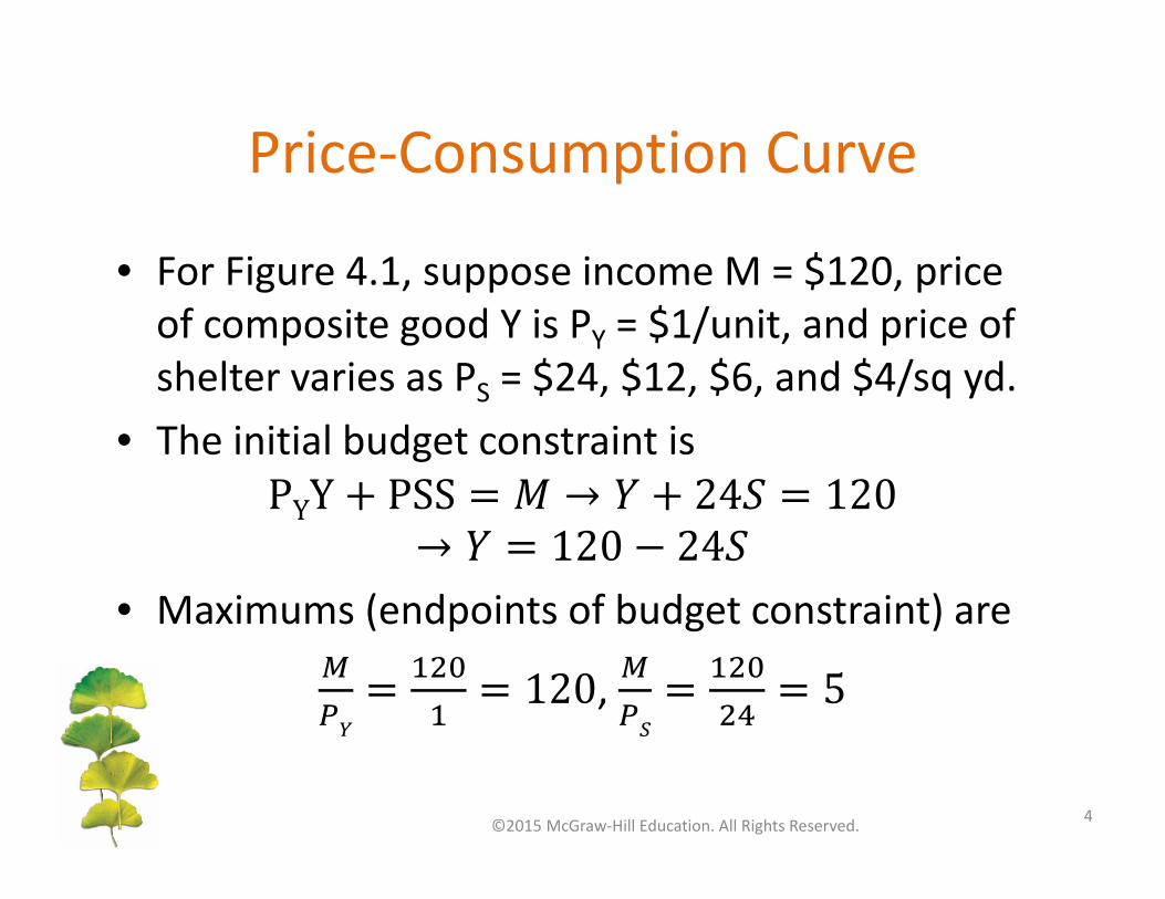
• For Figure 4.1, suppose income M = $120, price of composite good Y is PY = $1/unit, and price of shelter varies as PS = $24, $12, $6, and $4/sq yd.
• The initial budget constraint is
Y
• Maximums (endpoints of budget constraint) are
,
©2015 McGraw‐Hill Education. All Rights Reserved. 4
Price‐Consumption Curve
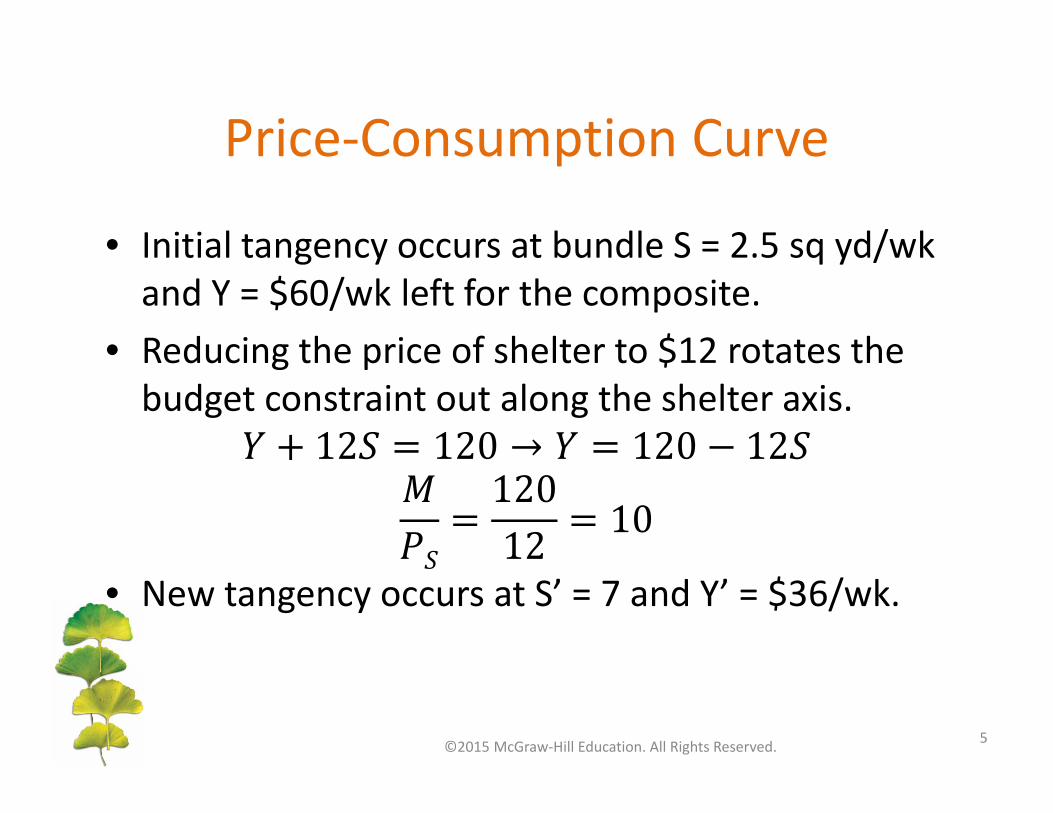
• Initial tangency occurs at bundle S = 2.5 sq yd/wkand Y = $60/wk left for the composite.
• Reducing the price of shelter to $12 rotates the budget constraint out along the shelter axis.
• New tangency occurs at S’ = 7 and Y’ = $36/wk.
©2015 McGraw‐Hill Education. All Rights Reserved. 5

Price‐Consumption Curve
• Repeat these steps for additional price reductions.– At PS = 6, consume S’’ = 15 and Y’’ = 30/wk.
– At PS = 4, consume S’’’ = 20 and Y’’’ = 40/wk.
• Connect the best affordable bundles (points of tangency) to construct the PCC.– Exhibits common pattern of a dip then recovery.
©2015 McGraw‐Hill Education. All Rights Reserved. 6
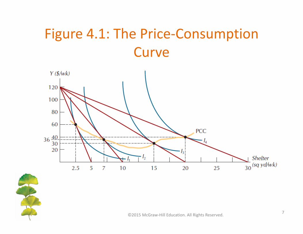
Figure 4.1: The Price‐Consumption Curve
©2015 McGraw‐Hill Education. All Rights Reserved. 7

Demand SchedulePrice of Shelter ($/sq yd) Quantity of Shelter Demanded (sq yd/wk)
24 2.5
12 7
6 15
4 20
• Construct by graphing the quantity of shelter demanded S (horizontal axis) versus the price of shelter PS (vertical axis) using PCC numbers, such as (S, PS) = (2.5, 24), (7, 12), (15, 6), (20, 4).
©2015 McGraw‐Hill Education. All Rights Reserved. 8
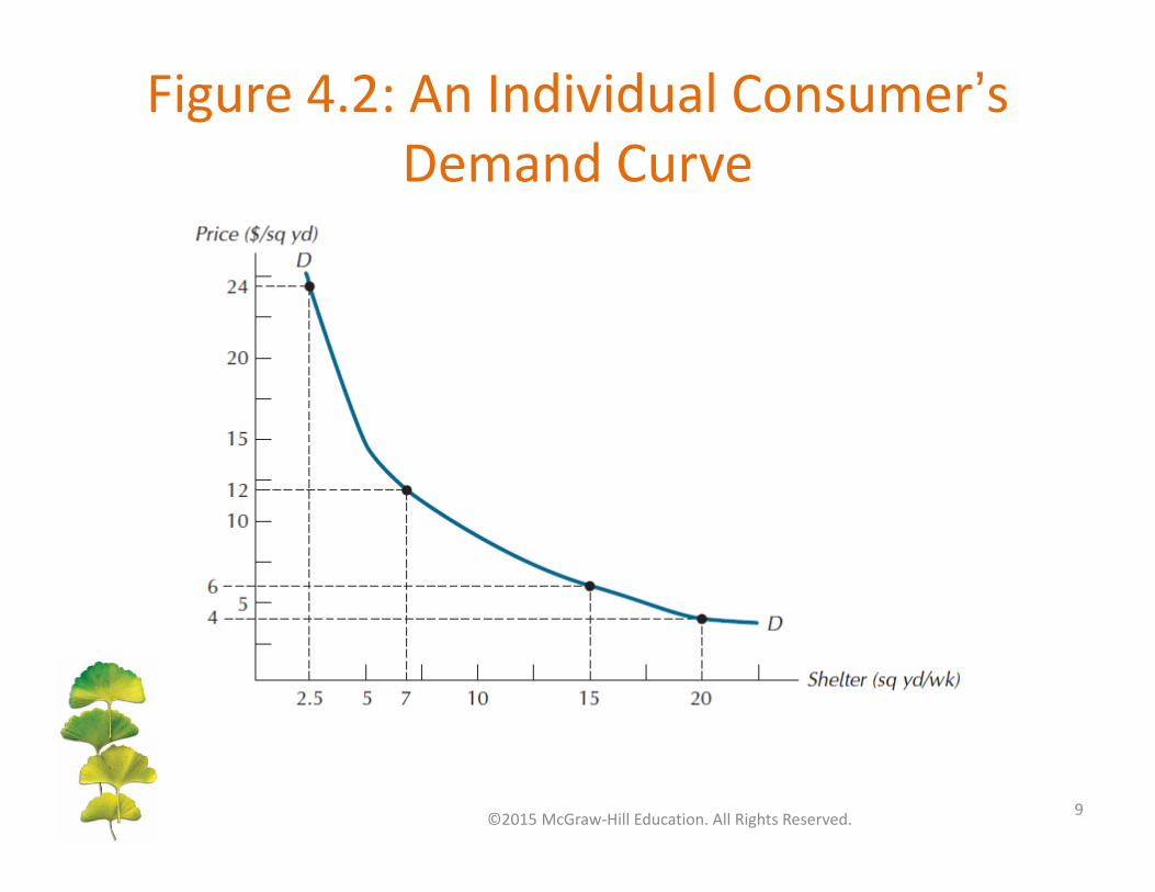
Figure 4.2: An Individual Consumer’s Demand Curve
©2015 McGraw‐Hill Education. All Rights Reserved. 9
The Effects of Changes in Income
©2015 McGraw‐Hill Education. All Rights Reserved. 10
• Income‐consumption curve (ICC): for a good X is the set of optimal bundles traced on an indifference map as income varies (holding the prices of X and Y constant).
• Engel curve: curve that plots the relationship between the quantity of X consumed and income.

Income‐Consumption Curve
• For Figure 4.3, suppose the price of shelter is PS = $10/sq yd, the price of the composite good is PY = $1, and income varies M = $40, $60, $100, $120.
• The initial budget constraint is
• Maximums (endpoints of budget constraint) are
,
• Initial tangency occurs at bundle S = 2 sq yd/wkand Y = $20/wk left for the composite.
©2015 McGraw‐Hill Education. All Rights Reserved. 11
Income‐Consumption Curve
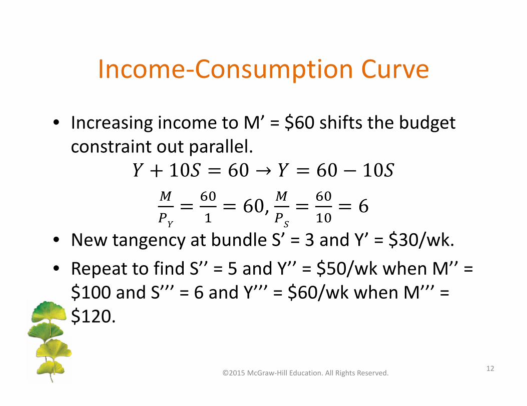
• Increasing income to M’ = $60 shifts the budget constraint out parallel.
,
• New tangency at bundle S’ = 3 and Y’ = $30/wk.
• Repeat to find S’’ = 5 and Y’’ = $50/wk when M’’ = $100 and S’’’ = 6 and Y’’’ = $60/wk when M’’’ = $120.
©2015 McGraw‐Hill Education. All Rights Reserved. 12

Income‐Consumption Curve
• Connect the best affordable bundles (points of tangency) to form the ICC.– It will have a positive slope if a normal good, where quantity demanded increases with income.
©2015 McGraw‐Hill Education. All Rights Reserved. 13
Income ($/wk) Quantity of shelter demanded (sq yd/wk)
40 2
60 3
100 5
120 6
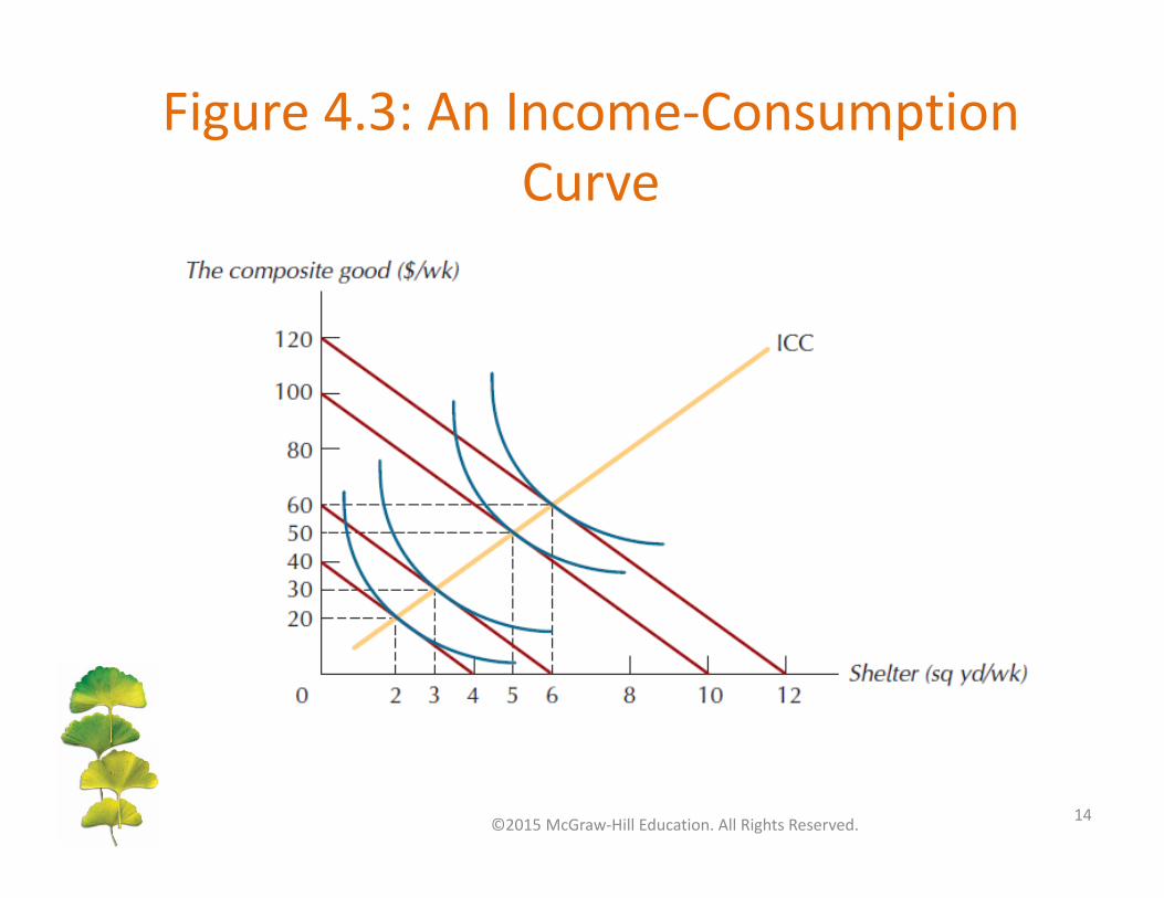
Figure 4.3: An Income‐Consumption Curve
©2015 McGraw‐Hill Education. All Rights Reserved. 14

Figure 4.4: An Individual Consumer’s Engel Curve
©2015 McGraw‐Hill Education. All Rights Reserved. 15

The Effects of Changes in Income
©2015 McGraw‐Hill Education. All Rights Reserved. 16
• Normal good: one whose quantity demanded rises as income rises.
• Inferior good: one whose quantity demanded falls as income rises.

Figure 4.5: The Engel Curve for Normal and Inferior Goods
©2015 McGraw‐Hill Education. All Rights Reserved. 17

Total Effect of a Price Increase
• For Figure 4.6, suppose PY = $1, M = $120, the price of shelter is initially PS = $6/sq yd and then increases to $24/sq yd.
• Initial budget constraint and endpoints are
,
• Tangency at initial consumption bundle S = 10 sq yd/wk and Y = $60/wk (point A).
©2015 McGraw‐Hill Education. All Rights Reserved. 18

Total Effect of a Price Increase
• When price of shelter increases to $24/sq yd, the new budget constraint and endpoints become
, 5
• Tangency at new consumption bundle S’ = 2 sqyd/wk and Y’ = $72/wk (point D).
• The total effect on the quantity demanded of shelter is a reduction of 10 – 2 = 8 sq yd/wk.
©2015 McGraw‐Hill Education. All Rights Reserved. 19

Figure 4.6: The Total Effectof a Price Increase
©2015 McGraw‐Hill Education. All Rights Reserved. 20

Income and Substitution Effects of a Price Change
©2015 McGraw‐Hill Education. All Rights Reserved. 21
• Substitution effect: that component of the total effect of a price change that results from the associated change in the relative attractiveness of other goods.
• Income effect: that component of the total effect of a price change that results from the associated change in real purchasing power.
• Total effect: the sum of the substitution and income effects.
Income and Substitution Effects
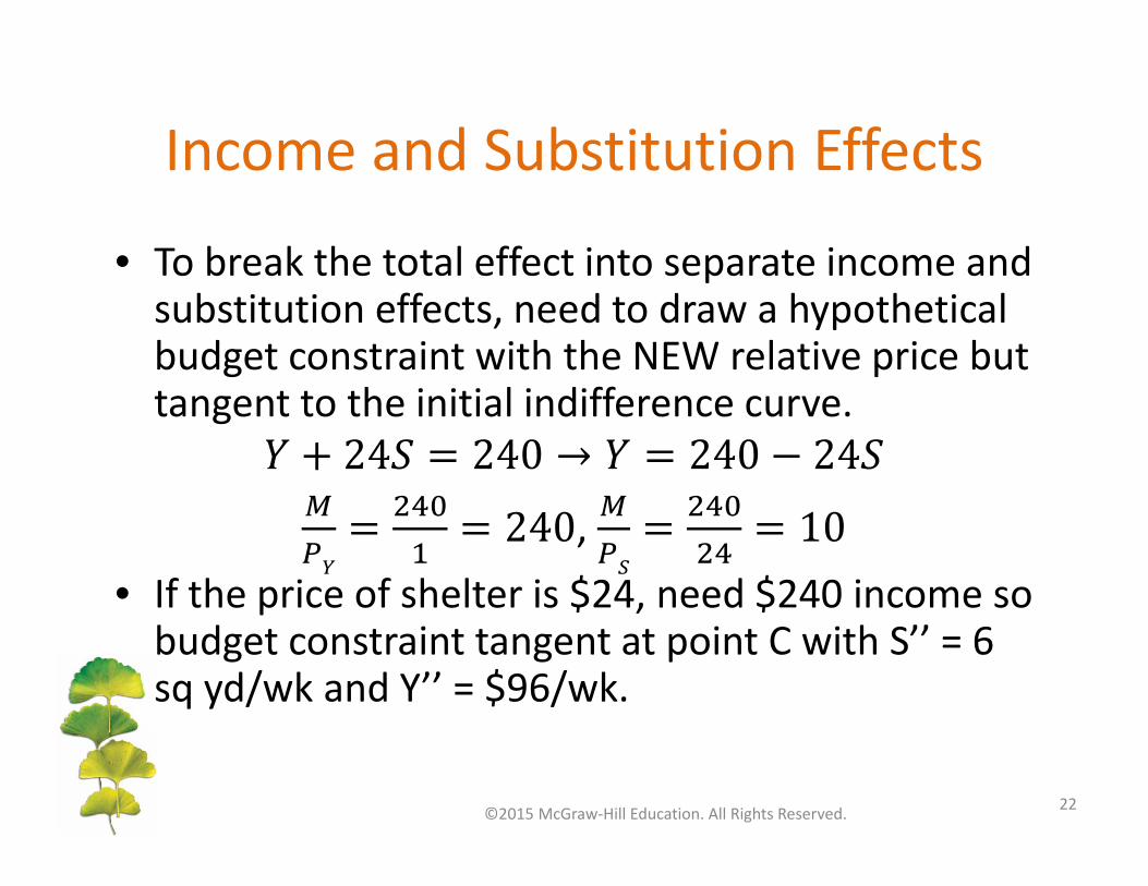
• To break the total effect into separate income and substitution effects, need to draw a hypothetical budget constraint with the NEW relative price but tangent to the initial indifference curve.
,
• If the price of shelter is $24, need $240 income so budget constraint tangent at point C with S’’ = 6 sq yd/wk and Y’’ = $96/wk.
©2015 McGraw‐Hill Education. All Rights Reserved. 22
Income and Substitution Effects
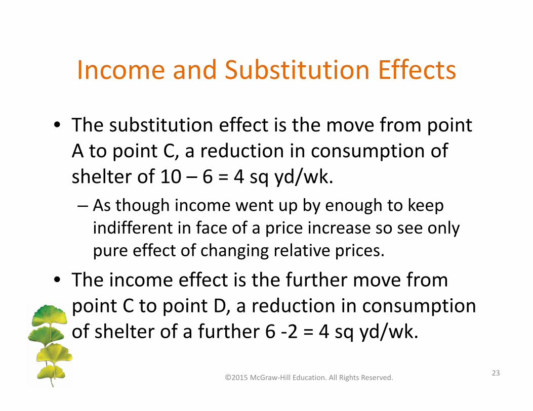
• The substitution effect is the move from point A to point C, a reduction in consumption of shelter of 10 – 6 = 4 sq yd/wk.– As though income went up by enough to keep indifferent in face of a price increase so see only pure effect of changing relative prices.
• The income effect is the further move from point C to point D, a reduction in consumption of shelter of a further 6 ‐2 = 4 sq yd/wk.
©2015 McGraw‐Hill Education. All Rights Reserved. 23

Figure 4.7: The Substitution and Income Effects of a Price Change
©2015 McGraw‐Hill Education. All Rights Reserved. 24

Income and Substitution Effects
Price Increase Normal Good Inferior Good
Substitution Effect ‐ ‐
Income Effect ‐ +
Total Effect ‐ +/‐
• For an increase in price of a good, the substitution effect causes quantity demanded to fall.– The income effect causes quantity demanded to fall for
a normal good but rise for an inferior good. – The total effect is a decrease in quantity demanded
unless an inferior good and the income effect dominates substitution effect.
©2015 McGraw‐Hill Education. All Rights Reserved. 25
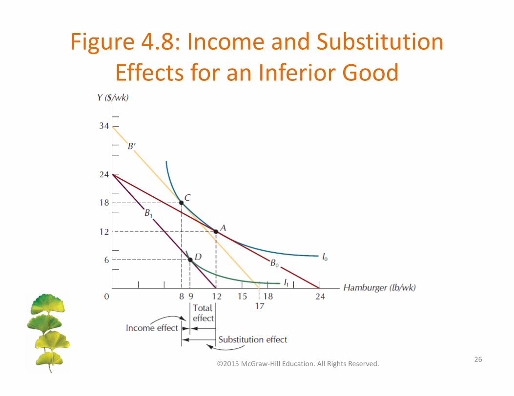
Figure 4.8: Income and Substitution Effects for an Inferior Good
©2015 McGraw‐Hill Education. All Rights Reserved. 26

Giffen Goods
©2015 McGraw‐Hill Education. All Rights Reserved. 27
• Giffen good: one for which the quantity demanded rises as its price rises.– The Giffen good must be an inferior good
– Income effect dominates substitution effect

Figure 4.9: The Demand Curvefor a Giffen Good
©2015 McGraw‐Hill Education. All Rights Reserved. 28

IE & SE for Perfect Complements
• For Figure 4.10, suppose skis and bindings are perfect complements, consumed in a fixed one‐to‐one ratio. M = $1,200/yr and PB = PS = $200/pair.
• Initial budget constraint and endpoints
, • Number of pairs of bindings must equal pairs of skis B = S due to being perfect complements. Solving 200S + 200S = 1200 gives B = S = 3 pairs.
©2015 McGraw‐Hill Education. All Rights Reserved. 29
IE & SE for Perfect Complements
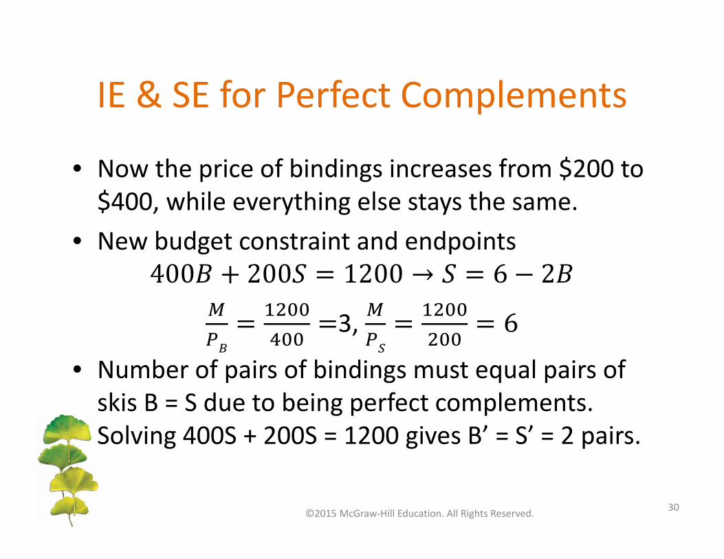
• Now the price of bindings increases from $200 to $400, while everything else stays the same.
• New budget constraint and endpoints
3,
• Number of pairs of bindings must equal pairs of skis B = S due to being perfect complements. Solving 400S + 200S = 1200 gives B’ = S’ = 2 pairs.
©2015 McGraw‐Hill Education. All Rights Reserved. 30
IE & SE for Perfect Complements
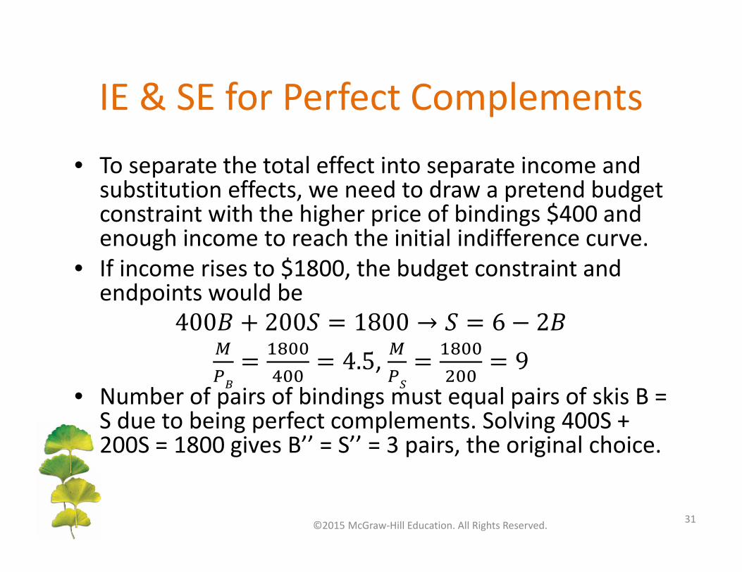
• To separate the total effect into separate income and substitution effects, we need to draw a pretend budget constraint with the higher price of bindings $400 and enough income to reach the initial indifference curve.
• If income rises to $1800, the budget constraint and endpoints would be
, • Number of pairs of bindings must equal pairs of skis B = S due to being perfect complements. Solving 400S + 200S = 1800 gives B’’ = S’’ = 3 pairs, the original choice.
©2015 McGraw‐Hill Education. All Rights Reserved. 31
IE & SE for Perfect Complements
• The substitution effect, the move from point A to point C due to higher price of bindings but with income compensated, is zero for perfect complements. – No ability to adjust mix of the two goods in response to changes in relative prices.
• The income effect, the move from point C to point D due to the higher price making bundles less affordable, is the full total effect, a reduction of one pair of bindings.
©2015 McGraw‐Hill Education. All Rights Reserved. 32

Figure 4.10: Income and Substitution Effects for Perfect Complements
©2015 McGraw‐Hill Education. All Rights Reserved. 33

IE & SE for Perfect Substitutes
• For Figure 4.11, suppose tea and coffee are perfect substitutes in a one‐to‐one ratio (one cup of coffee is a good as one cup of tea). M = $12/wk, PC = $1/cup and PT = $1.20/cup.
• Initial budget constraint and endpoints
, .
• Optimal bundle (point A) is 12 cups of coffee (and no tea), which is equivalent in satisfaction to 12 cups of tea (and no coffee).
©2015 McGraw‐Hill Education. All Rights Reserved. 34

IE & SE for Perfect Substitutes
• Now suppose the price of coffee increases from $1 to $1.50/cup, while all else remains the same.
• New budget constraint and endpoints
.,
.• Optimal bundle (point D) is 10 cups of tea (with no coffee), which is equivalent in satisfaction to 10 cups of coffee (with no tea).
©2015 McGraw‐Hill Education. All Rights Reserved. 35

IE & SE for Perfect Substitutes
• Construct budget constraint with the higher price of coffee and enough income to reach initial indifference curve.
• New budget constraint and endpoints
..
, ..
2• Need an additional $2.40 to afford two more cups of tea so point C is 12 cups of tea (with no coffee), which is equivalent in satisfaction to the original 12 cups of coffee (with no tea).
©2015 McGraw‐Hill Education. All Rights Reserved. 36

IE & SE for Perfect Substitutes
• Substitution effect is a dramatic reduction in coffee consumption of 12 – 0 = 12 cups, the total effect.
• Substitution effects for perfect substitutes can be very large if they induce a switch from one good to the other.
©2015 McGraw‐Hill Education. All Rights Reserved. 37

Figure 4.11: Income and Substitution Effects for Perfect Substitutes
©2015 McGraw‐Hill Education. All Rights Reserved. 38

Demand for Car Washes
• For Figure 4.14, M = $144, PG = $3/gal. Buy 1 car wash for every 10 gallons of gas (G = 10C). Consider prices of car washes such as $6, $18 and $42 to construct individual demand curve.
,
3(10C) + 6C = 144, 36C = 144, C = 4, G = 40/wk
©2015 McGraw‐Hill Education. All Rights Reserved. 39

Demand for Car Washes
• When car washes cost $18
,
3(10C) + 18C = 144, 48C = 144, C = 3, G = 30/wk• When car washes cost $42
,
3(10C) + 42C = 144, 72C = 144, C = 2, G = 20/wk
©2015 McGraw‐Hill Education. All Rights Reserved. 40
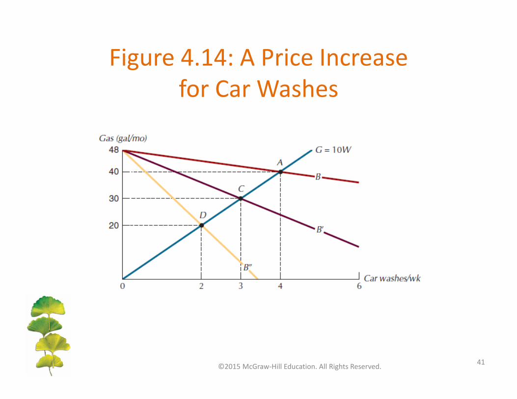
Figure 4.14: A Price Increasefor Car Washes
©2015 McGraw‐Hill Education. All Rights Reserved. 41
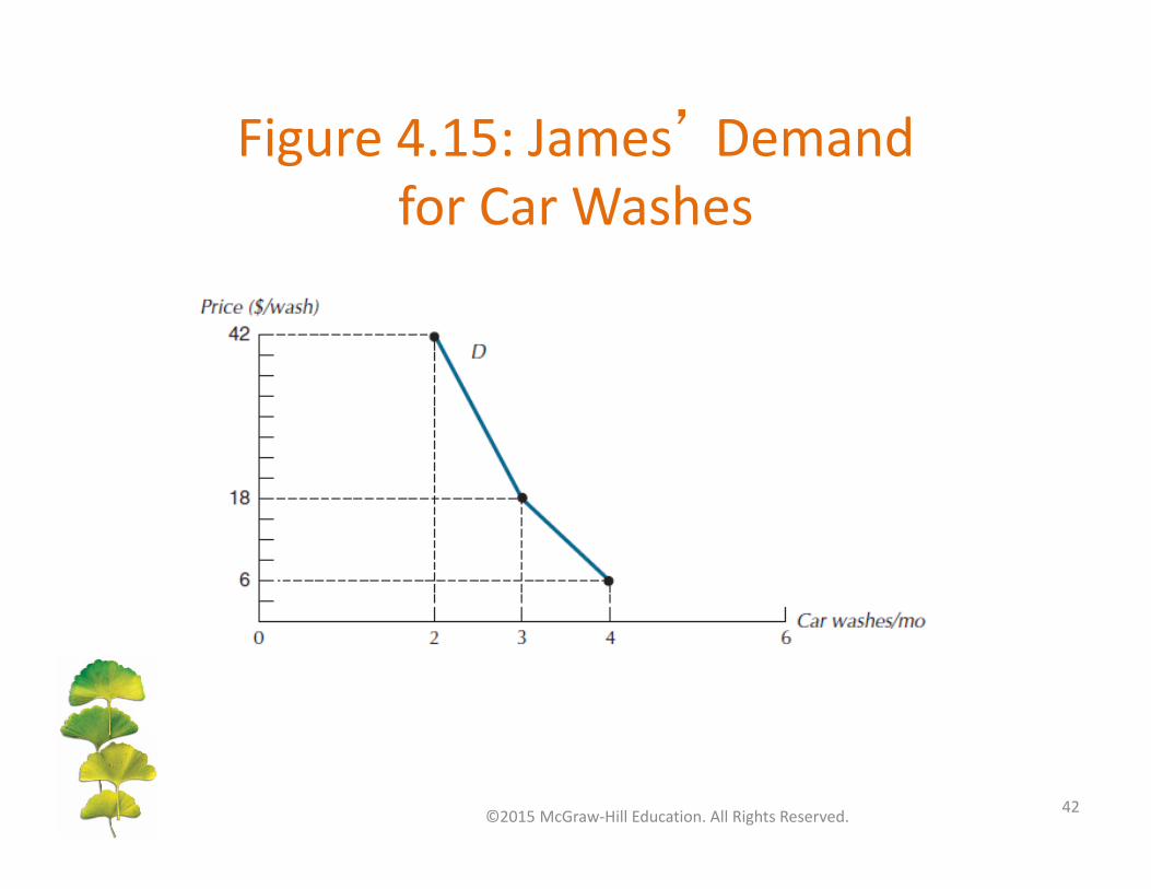
Figure 4.15: James’ Demandfor Car Washes
©2015 McGraw‐Hill Education. All Rights Reserved. 42

Market Demand Curves
©2015 McGraw‐Hill Education. All Rights Reserved. 43
• Market demand curve: the horizontal summation of the individual demand curves.
• .

Figure 4.16: Generating Market Demand from Individual Demands
©2015 McGraw‐Hill Education. All Rights Reserved. 44
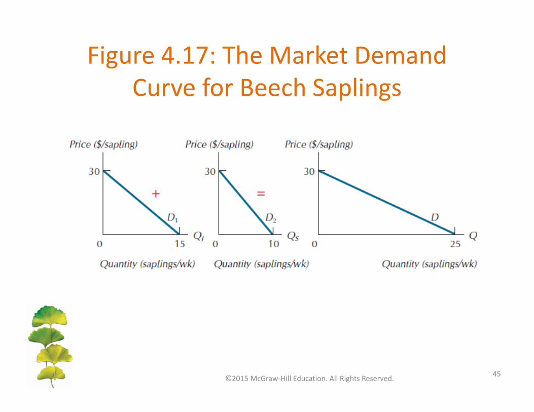
Figure 4.17: The Market Demand Curve for Beech Saplings
©2015 McGraw‐Hill Education. All Rights Reserved. 45
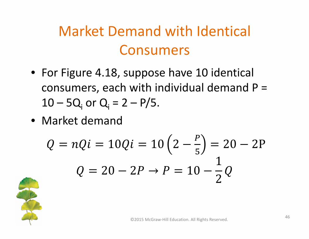
Market Demand with Identical Consumers
• For Figure 4.18, suppose have 10 identical consumers, each with individual demand P = 10 – 5Qi or Qi = 2 – P/5.
• Market demand
©2015 McGraw‐Hill Education. All Rights Reserved. 46

Market Demand with Identical Consumers
• In general, for a market with n identical individual demand P = a – bQi, the market demand will be
©2015 McGraw‐Hill Education. All Rights Reserved. 47

Figure 4.18: Market Demand with Identical Consumers
©2015 McGraw‐Hill Education. All Rights Reserved. 48
Price Elasticity of Demand
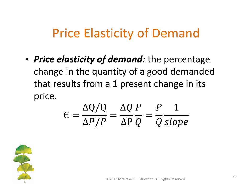
• Price elasticity of demand: the percentage change in the quantity of a good demanded that results from a 1 present change in its price.
Є
©2015 McGraw‐Hill Education. All Rights Reserved. 49
Three Categories of Price Elasticity
©2015 McGraw‐Hill Education. All Rights Reserved. 50
• Inelastic → |Є| < 1
• Elastic → |Є| > 1
• Unit elastic → |Є| = 1

Figure 4.19: Three Categoriesof Price Elasticity
©2015 McGraw‐Hill Education. All Rights Reserved. 51

Figure 4.20: The Point‐Slope Method
©2015 McGraw‐Hill Education. All Rights Reserved. 52

Figure 4.21: Two Important Polar Cases
©2015 McGraw‐Hill Education. All Rights Reserved. 53

Elasticity and Total Revenue
©2015 McGraw‐Hill Education. All Rights Reserved. 54
• A price reduction will increase total revenue if and only if the absolute value of the price elasticity of demand is greater than 1.
• An increase in price will increase total revenue if and only if the absolute value of the price elasticity is less than 1.

Figure 4.23: The Effect on Total Expenditure of a Reduction in Price
©2015 McGraw‐Hill Education. All Rights Reserved. 55
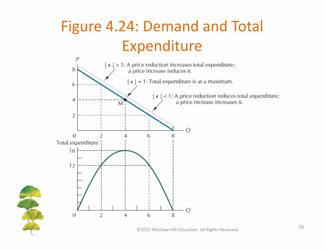
Figure 4.24: Demand and Total Expenditure
©2015 McGraw‐Hill Education. All Rights Reserved. 56

Demand for Bus Rides
• For Figure 4.25, P = 100 – Q/10. If P = 50 cents/ride (point M), how much revenue will be collected?
• What is the price elasticity of demand?
Є
• Should the system raise or lower prices to increase revenue? Neither, revenue is maximized (unit elasticity).
©2015 McGraw‐Hill Education. All Rights Reserved. 57

Demand for Bus Rides
• For P’ = 75 cents/ride (point K), how much revenue will be collected?
• What is the price elasticity of demand?
Є
• Should the system raise or lower prices to increase revenue? Lower prices (demand is elastic).
©2015 McGraw‐Hill Education. All Rights Reserved. 58
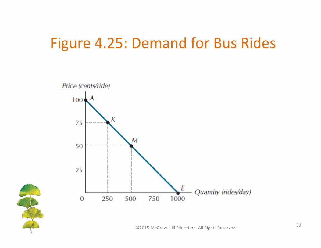
Figure 4.25: Demand for Bus Rides
©2015 McGraw‐Hill Education. All Rights Reserved. 59
Determinants of Price Elasticity of Demand
©2015 McGraw‐Hill Education. All Rights Reserved. 60
• Substitution possibilities: the substitution effect of a price change tends to be small for goods with no close substitutes.
• Budget share: the larger the share of total expenditures accounted for by the product, the more important will be the income effect of a price change.
• Direction of income effect: a normal good will have a higher price elasticity than an inferior good.
• Time: demand for a good will be more responsive to price in the long‐run than in the short‐run.
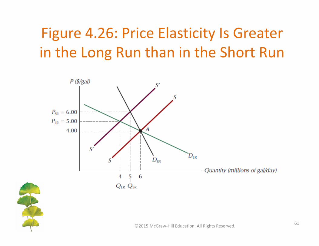
Figure 4.26: Price Elasticity Is Greater in the Long Run than in the Short Run
©2015 McGraw‐Hill Education. All Rights Reserved. 61
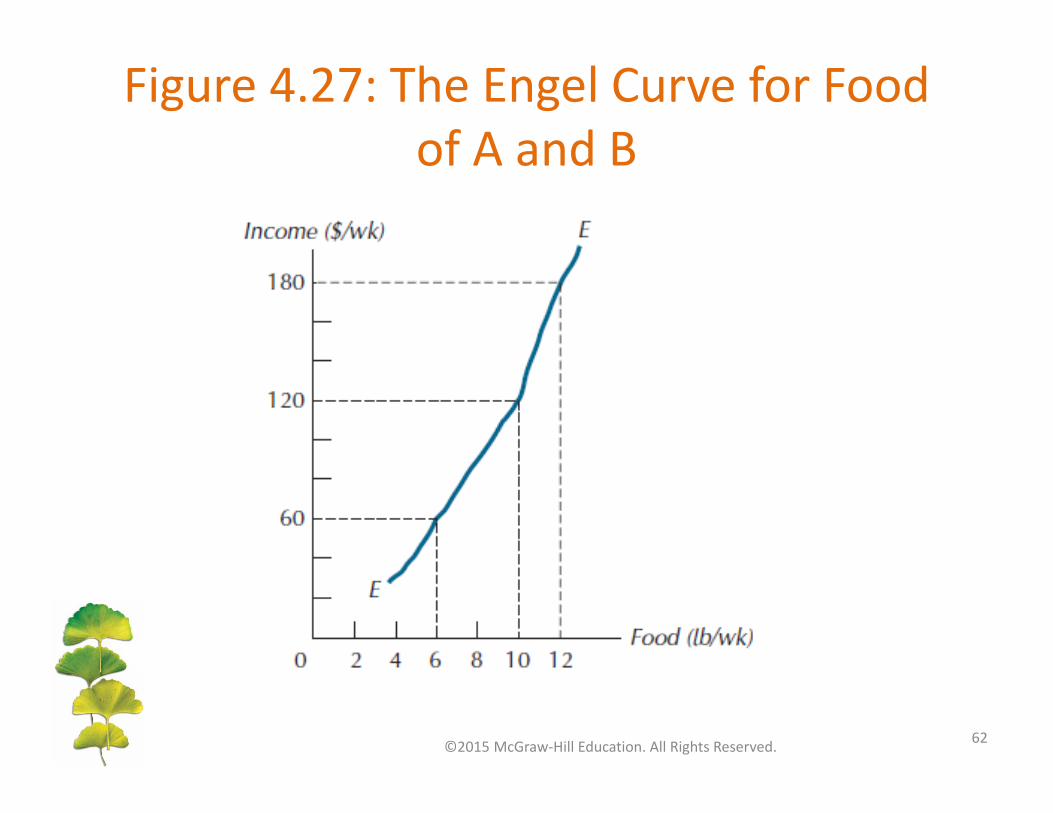
Figure 4.27: The Engel Curve for Foodof A and B
©2015 McGraw‐Hill Education. All Rights Reserved. 62
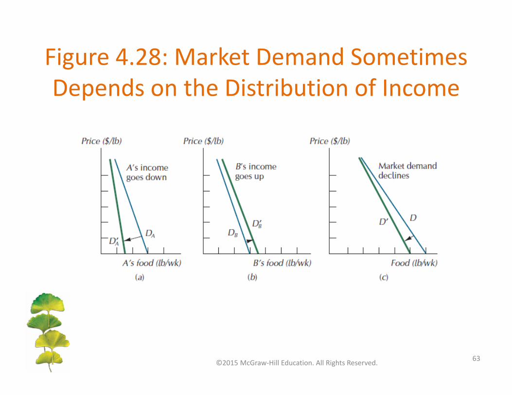
Figure 4.28: Market Demand Sometimes Depends on the Distribution of Income
©2015 McGraw‐Hill Education. All Rights Reserved. 63

Figure 4.29: An Engel Curveat the Market Level
©2015 McGraw‐Hill Education. All Rights Reserved. 64

Income Elasticity of Demand
• If a good exhibits a stable Engle curve, we can define its income elasticity of demand, the percentage change in the quantity of a good demanded that results from a 1 percent change in income.
©2015 McGraw‐Hill Education. All Rights Reserved. 65
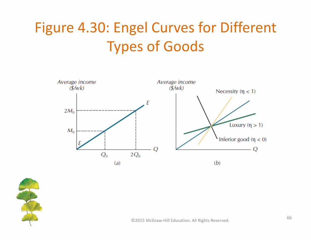
©2015 McGraw‐Hill Education. All Rights Reserved. 66
Figure 4.30: Engel Curves for Different Types of Goods

Cross‐Price Elasticities of Demand
• Cross‐price elasticity of demand: the percentage change in the quantity of one good demanded that results from a 1 percent change in the price of the other good.
©2015 McGraw‐Hill Education. All Rights Reserved. 67
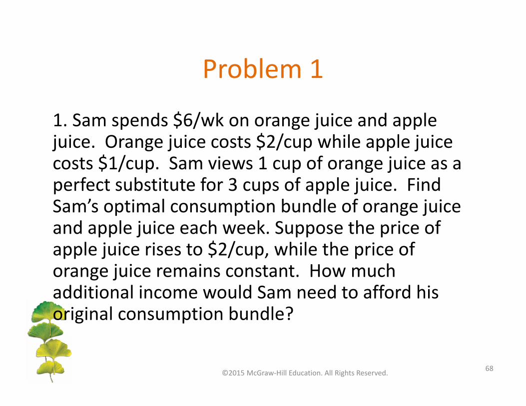
Problem 1
1. Sam spends $6/wk on orange juice and apple juice. Orange juice costs $2/cup while apple juice costs $1/cup. Sam views 1 cup of orange juice as a perfect substitute for 3 cups of apple juice. Find Sam’s optimal consumption bundle of orange juice and apple juice each week. Suppose the price of apple juice rises to $2/cup, while the price of orange juice remains constant. How much additional income would Sam need to afford his original consumption bundle?
©2015 McGraw‐Hill Education. All Rights Reserved. 68

Solution 1
• Budget constraint and endpoints
,
• Optimal consumption bundle is 3 cups of orange juice (and no apple juice), which viewed as good as 9 cups of apple juice (and no orange juice).
• If the price of apple juice doubles from $1 to $2/cup, Sam would not need any additional income as he was not consuming any apple juice.
©2015 McGraw‐Hill Education. All Rights Reserved. 69

Solution 1 Figure
0
3
6
9
0 3
App
le Ju
ice (cup
s)
Orange Juice (cups)
B0
B1
I0
©2015 McGraw‐Hill Education. All Rights Reserved. 70

Problem 2
2. Maureen has the same income and faces the same prices as Sam, but Maureen views 1 cup of orange juice and 1 cup of apple juice as perfect complements. Find Maureen’s optimal consumption bundle. How much additional income would Maureen need to afford her original consumption bundle when the price of apple juice doubles?
©2015 McGraw‐Hill Education. All Rights Reserved. 71
Solution 2
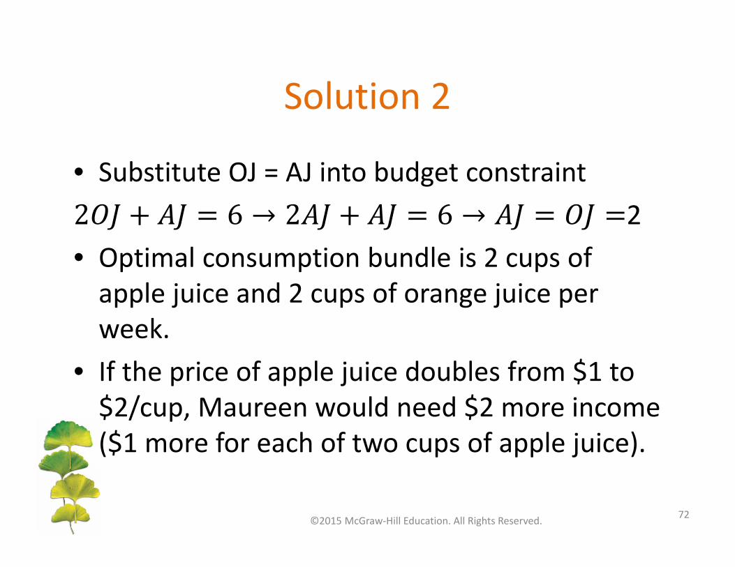
• Substitute OJ = AJ into budget constraint
2
• Optimal consumption bundle is 2 cups of apple juice and 2 cups of orange juice per week.
• If the price of apple juice doubles from $1 to $2/cup, Maureen would need $2 more income ($1 more for each of two cups of apple juice).
©2015 McGraw‐Hill Education. All Rights Reserved. 72

Solution 2 Figure
0
1
2
3
4
5
6
0 1 2 3 4
App
le Ju
ice (cup
s)
Orange Juice (cups)
B0
B1
I0AJ=OJ
B2
©2015 McGraw‐Hill Education. All Rights Reserved. 73

Problem 3
3. Suppose the demand for crossing the Golden Gate Bridge is given by Q = 10,000 ‐ 1000P. a. If the toll (P) is $2, how much revenue is collected?b. What is the price elasticity of demand at this point?c. Could the bridge authorities increase their revenues by changing their price?d. The Red and White Lines, a ferry service that competes with the Golden Gate Bridge, began operating hovercrafts that made commuting by ferry much more convenient. How would this affect the elasticity of demand for trips across the Golden Gate Bridge?
©2015 McGraw‐Hill Education. All Rights Reserved. 74
Solution 3
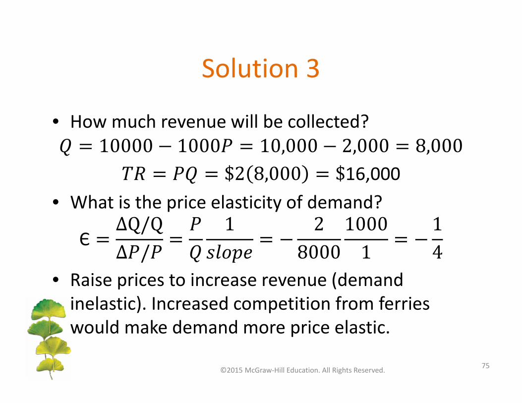
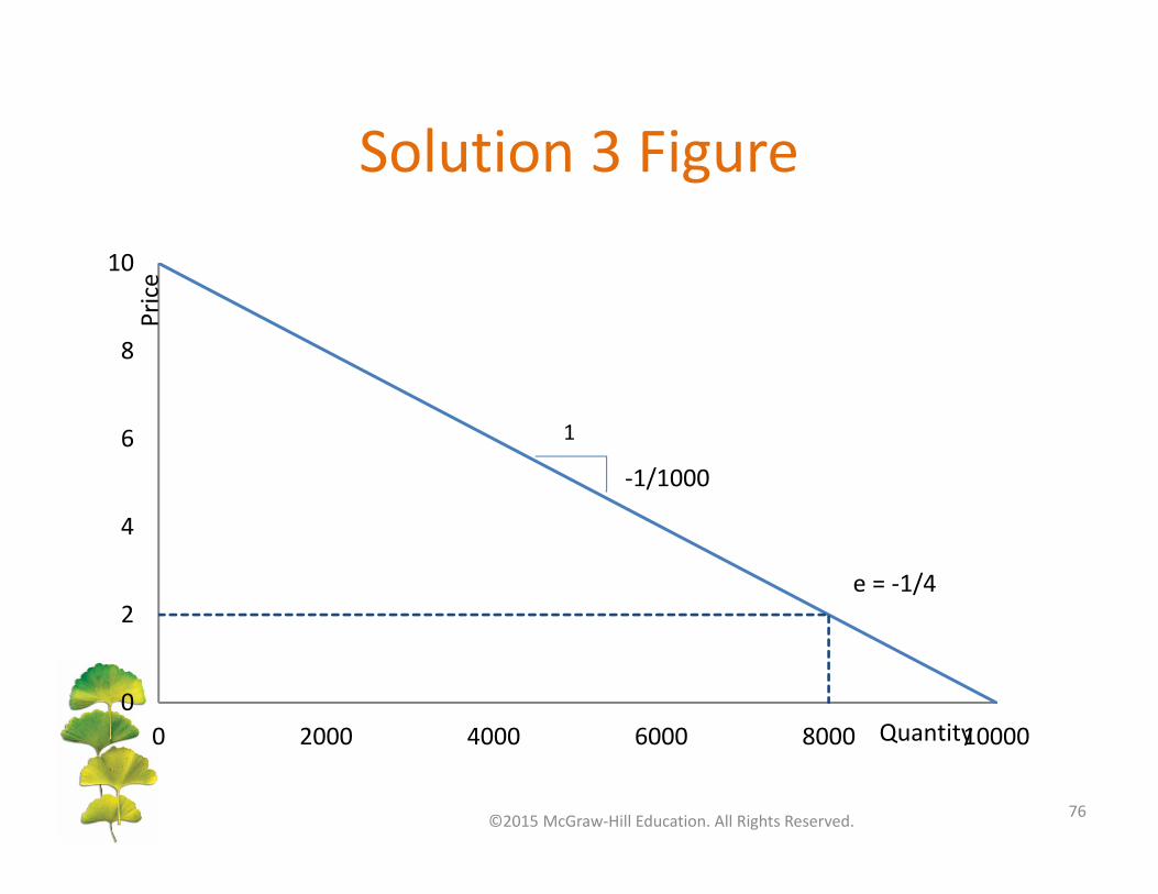
• How much revenue will be collected?
16,000
• What is the price elasticity of demand?
Є
• Raise prices to increase revenue (demand inelastic). Increased competition from ferries would make demand more price elastic.
©2015 McGraw‐Hill Education. All Rights Reserved. 75
Solution 3 Figure
0
2
4
6
8
10
0 2000 4000 6000 8000 10000
Price
Quantity
e = ‐1/4
1
‐1/1000
©2015 McGraw‐Hill Education. All Rights Reserved. 76

Problem 4
4. Professors Adams and Brown make up the entire demand side of the market for summer research assistants in the economics department. If Adam’s demand curve is P = 50 ‐2QA and Brown’s is P = 50 ‐ QB, where QA and QBare the hours demanded by Adams and Brown, respectively, what is the market demand for research hours in the economics department?
©2015 McGraw‐Hill Education. All Rights Reserved. 77

Solution 4
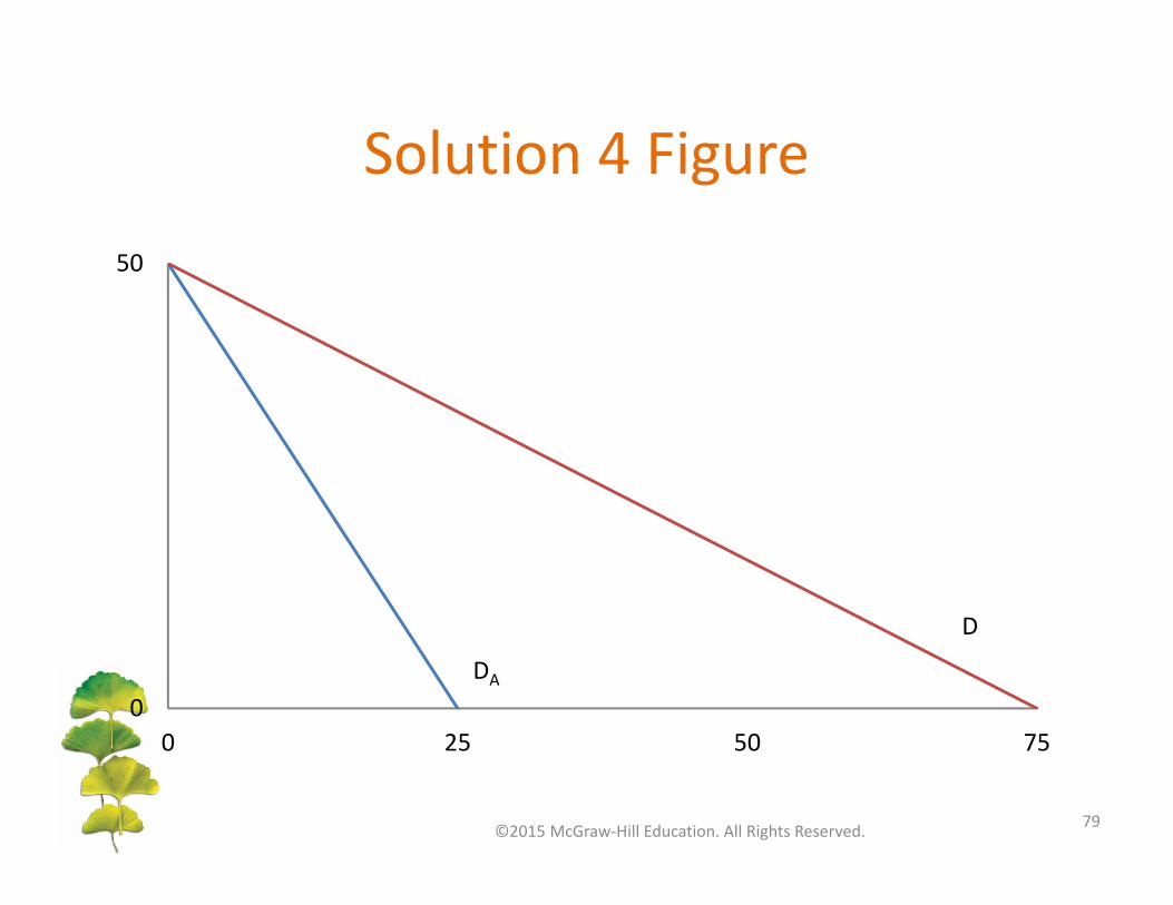
• Professor Adam (price intercept 50, Q intercept 25)
• Professor Brown (price intercept 50, Q intercept 50)
• Market demand (price intercept 50, Q intercept 75)
©2015 McGraw‐Hill Education. All Rights Reserved. 78
Solution 4 Figure
0
50
0 25 50 75
D
DA
©2015 McGraw‐Hill Education. All Rights Reserved. 79