individualising kinematic modelling in the gait analysis ... · ganganalyse en het bestuderen van...
TRANSCRIPT

Academic year 2013 - 2014
Individualising kinematic modelling in the gait
analysis of osteoarthritic knee patients Integration of 3D bone morphological segmentation methods with classic
kinematic modelling techniques
Heleen DAELEWIJN
and
Levi HOSTE
Promotors: F. Plasschaert MD, Phd and J. Victor MD, Phd
Co-promotors: M. Forward, Phd and C. Van Der Straeten MD, Phd
Master’s thesis submitted in the 2nd Master year in fulfillment of the requirements for the
degree of
MASTER OF MEDICINE IN DE GENEESKUNDE

Acknowledgments
This master’s thesis would not have been possible without the support of many people. First
and foremost, we would like to express our sincere gratitude to our promoters and co-
promotors, Frank Plasschaert (MD, Phd), Jan Victor (MD, Phd), Malcolm Forward (Phd) and
Catherine Van Der Straeten (MD, Phd), for the great opportunity to be part of this research and
use it for our thesis.
Our special thanks goes out to Prof. Malcolm Forward for his guidance, patience, motivation
and knowledge throughout every step of this thesis for the past two years. His valuable and
constructive suggestions during the planning and development of this research work and his
willingness to give his time so generously has been very much appreciated.
We would also like to thank Prof. Catherine Van Der Straeten MD in special for the help in
recruiting the patients, keeping our progress on schedule and giving great advice in the further
development of this thesis.
We are particularly grateful for the assistance given by Prof. Jan Victor MD and his research
work on the subject of knee alignment. His previous publications have been a great base for
our own research on this matter.
Furthermore, we highly appreciate the assistance provided by all the staff members of the
Departments of Orthopaedics and Traumatology, Radiology and especially those of the
Cerebral Palsy Reference Centre at the University Hospital of Ghent. In special, we would like
to thank Ellen De Dobbelaere for her training and assistance in the gait lab.
At last, a personal word of gratitude goes out to Emma Dejonghe and Henri Himpe, both close
to us, for the great support and encouragement throughout our studies.

Table of contents
ABSTRACT (ENGLISH) ..................................................................................................................................... 1
ABSTRACT (NEDERLANDS) ........................................................................................................................... 2
INTRODUCTION ................................................................................................................................................ 3
RESEARCH PROBLEM DESCRIPTION ..................................................................................................................... 3 THESIS OVERVIEW ............................................................................................................................................... 6
1. BACKGROUND .......................................................................................................................................... 7
1.1 KNEE OSTEOARTHRITIS .......................................................................................................................... 7 1.1.1 Pathogenesis of osteoarthritis .......................................................................................................... 7 1.1.2 Epidemiology .................................................................................................................................... 8 1.1.3 Treatment of osteoarthritis ............................................................................................................... 9
1.2 GAIT ANALYSIS .................................................................................................................................... 11 1.2.1 Definitions ...................................................................................................................................... 11
1.2.1.1 Locomotion and gait .............................................................................................................................. 11 1.2.1.2 Gait analysis ........................................................................................................................................... 11
1.2.2 Difficulties and restrictions ............................................................................................................ 12 1.3 GAIT IN PATIENTS WITH KNEE OSTEOARTHRITIS .................................................................................. 14
1.3.1 Common findings in knee OA patients ............................................................................................ 14 1.3.2 Common findings after total knee arthroplasty .............................................................................. 15
2. LITERATURE REVIEW ......................................................................................................................... 17
2.1 FINDINGS ............................................................................................................................................. 17 2.2 CONCLUSIONS AND RELEVANCE FOR EXPERIMENTAL WORK ................................................................ 18
3. EXPERIMENTAL EVALUATION ......................................................................................................... 19
3.1 MATERIAL AND METHODS .................................................................................................................... 19 3.1.1 Study design and selection .............................................................................................................. 19 3.1.2 Study procedures and data collection ............................................................................................. 19
3.1.2.1 Gait assessment ...................................................................................................................................... 20 3.1.2.1.1 Introduction and preparation .......................................................................................................... 20 3.1.2.1.2 Plates with extra markers ............................................................................................................... 20 3.1.2.1.3 Gait assessment.............................................................................................................................. 23 3.1.2.1.4 Gait analysis .................................................................................................................................. 23
3.1.2.2 Medical imaging .................................................................................................................................... 24 3.1.2.2.1 Radiology ...................................................................................................................................... 24 3.1.2.2.2 Segmenting of CT slices in Mimics ............................................................................................... 24 3.1.2.2.3 Readings in 3-matic ....................................................................................................................... 25
3.1.2.3 CT-based subject-specific gait model .................................................................................................... 25 3.1.2.4 Intermezzo: Assessing the reliability of the data collection ................................................................... 25
3.1.3 Statistical analysis .......................................................................................................................... 25 3.2 RESULTS .............................................................................................................................................. 27
3.2.1 Study subjects.................................................................................................................................. 27 3.2.2 Comparison of the generic model with a replica ............................................................................ 27 3.2.3 Comparison of the generic model with a subject-specific CT-based model ................................... 29
3.2.3.1 Comparison of the kinematics ................................................................................................................ 29 3.2.3.2 Comparison of the positions of anatomical landmarks ........................................................................... 34
3.2.3.2.1 Hip joint centres............................................................................................................................. 34 3.2.3.2.2 Knee joint centres .......................................................................................................................... 37
3.2.4 Comparison of the pre and post-surgical assessments ................................................................... 37 3.2.4.1 Comparison of the temporal gait parameters .......................................................................................... 38 3.2.4.2 Comparison of the kinematics ................................................................................................................ 39
3.2.4.2.1 PIG ................................................................................................................................................ 39 3.2.4.2.2 CTM .............................................................................................................................................. 39
3.3 DISCUSSION ......................................................................................................................................... 40

3.3.1 Methodological considerations ....................................................................................................... 40 3.3.2 Health economics ............................................................................................................................ 41 3.3.3 Radiation dose ................................................................................................................................ 41 3.3.4 Conclusions and future work .......................................................................................................... 42
LIST OF FIGURES ............................................................................................................................................ 45
LIST OF TABLES .............................................................................................................................................. 45
REFERENCES ................................................................................................................................................... 47
APPENDICES ..................................................................................................................................................... 51
APPENDIX 1 : KELLGREN-LAWRENCE GRADING SCALE .................................................................................... 51 APPENDIX 2 : MIMICS AND 3-MATIC MANUAL ................................................................................................... 51 APPENDIX 3 : DIMENSIONS OF THE TIBIAL PLATE .............................................................................................. 55 APPENDIX 4 : DIMENSIONS OF THE SACRAL PLATE ............................................................................................ 56 APPENDIX 5 : ASSESSMENT OF RELIABILITY OF GAIT LAB DATA ........................................................................ 57 APPENDIX 6 : KINEMATIC GRAPHS COMPARING THE PLUG-IN-GAIT WITH THE REPLICA MODEL........................ 61 APPENDIX 7 : SUMMARY KINEMATIC VARIABLES AND THEIR COMPARISON BETWEEN THE GENERIC PIG-MODEL
AND THE REPLICA MODEL .................................................................................................................................. 67 APPENDIX 8 : KINEMATIC GRAPHS COMPARING THE PLUG-IN-GAIT WITH THE CT-MODEL ............................... 68 APPENDIX 9 : SUMMARY KINEMATIC VARIABLES AND THE COMPARISON BETWEEN THE PIG MODEL AND THE
CTM: SYSTEMATIC DIFFERENCES BY T-TESTING .............................................................................................. 71 APPENDIX 10 : SUMMARY KINEMATIC VARIABLES AND THE COMPARISON BETWEEN THE PIG MODEL AND THE
CTM: CORRELATION AND AGREEMENT TESTING .............................................................................................. 72 APPENDIX 11 : TEMPORAL PARAMETERS PRE- AND POST-SURGERY .................................................................. 73 APPENDIX 12 : SUMMARY KINEMATIC VARIABLES AND THE COMPARISON BETWEEN PRE- AND POST-SURGICALLY:
SYSTEMATIC DIFFERENCES BY T-TESTING ........................................................................................................ 74

Abstract (English)
1
Abstract (English)
Among older adults, osteoarthritis (OA) is the most common cause of walking-related
disability and the main source for total knee arthroplasty (TKA) in Western countries. Over the
past decade, TKA has developed to a complete functional and pain free result therapy.
Nevertheless, a large variation in the outcome of total knee arthroplasty procedures is still
observed. Gait analysis and the study of patient-specific kinematics and kinetics could provide
an answer to this puzzle.
Most of the software packages in gait analysis rely on a rescaled generic model of the lower
extremity. Nevertheless, this procedure can induce major errors, mainly due to (1) errors
associated with marker placement on anatomical landmarks and (2) imprecision in the
description of joint systems. This is especially so because of particular problems around the
pelvis and knee and in obese patients.
In this pilot study, where three elderly TKA patients were included, an alternative, hybrid
model was built based on information of computer tomography (CT) images of the patients.
By running this adapted, subject-specific model, joint centres, kinetics and kinematics were
redefined. We hypothesized that the kinematics calculated with the CT-model would be more
accurate and individually correct than those based on the generic Plug-in-Gait (PIG) model.
Three patients, of whom two were clinically obese, underwent a complete gait assessment, both
before and after their TKA. Major kinematic differences were found between the generic and
the subject-specific model, especially when obesity was present. Specifically hip (sagittal and
transverse) and knee (sagittal ROM, frontal and transverse) kinematics were clearly different
between the models. In the obese, pelvic differences stood out. Poor correlations were found
between the models, but they differed individually. The positions of the CT-based and generic
hip and knee joint centres diverged on a surprisingly large scale. The CT-based hip centres
were found not only different, but also more accurate according to empirical data provided by
Bell et al. Post-surgically, walking speed drastically increased in the pain free patients. In these
patients also sagittal hip and knee ROM exhibited a clear increase.
In conclusion, it was found that a rescaled, generic gait model is incapable of accurately
describing kinematic patterns in elderly knee patients. Especially when obesity is present, the
differences between the models mount up. Medical imaging-based models could provide an
answer as particularly hip and knee kinematics improve in accuracy.

Abstract (Nederlands)
2
Abstract (Nederlands) Osteoartritis is één van de belangrijkste oorzaken van problemen bij het wandelen bij ouderen.
Het is in de Westerse wereld bovendien de hoofdreden voor een totale knie prothese (TKP).
De afgelopen tien jaar is TKP geëvolueerd naar een compleet functionele therapie met vaak
een pijnvrij resultaat. Toch is er nog steeds een grote variatie in de uitkomsten en tevredenheid
van TKP. Ganganalyse en het bestuderen van patiëntspecifieke kinematica en kinetica zouden
een oplossing kunnen bieden voor deze problematiek.
Heden zijn de meeste softwarepakketten bij ganganalyses gebaseerd op een geschaald
generisch model van de onderste ledematen. Deze procedure leidt tot grote fouten, vooral toe
te wijzen aan (1) moeilijkheden bij het plaatsen van markers op anatomische referentiepunten
en (2) onnauwkeurigheid bij het bepalen van de gewrichten. Deze onnauwkeurigheden komen
des te meer tot uiting ter hoogte van het bekken en de knie, vooral bij obese patiënten.
In deze pilootstudie, waar drie oudere TKP patiënten werden geïncludeerd, werd een
alternatief, hybride model ontwikkeld op basis van computertomografie (CT) beelden. Via dit
aangepast, patiëntspecifiek model werden de kinetica en kinematica herbepaald. Er werd
gesteld dat de kinematica berekend via het CT-model meer accuraat en individueel correct
zouden zijn dan de kinematica gebaseerd op het generische Plug-in-Gait (PIG) model.
Drie patiënten, waarvan twee obees, ondergingen een volledige ganganalyse, zowel vóór als
na hun TKP. Er werden grote kinematische verschillen gevonden tussen het generische en het
patiëntspecifieke model, vooral bij de obese patiënten. Ter hoogte van de heup (sagittale en
transversale kinematica) en de knie (sagittale ROM, frontale en transversale kinematica) waren
duidelijke verschillen te noteren tussen de modellen. Bij de obese patiënten werden bovendien
belangrijke verschillen ter hoogte van het bekken opgemerkt. De twee modellen waren slechts
zwak gecorreleerd, al was dit individueel sterk verschillend. De posities van de CT- en
generisch bepaalde heup- en kniegewrichtcentra verschilden sterk, waarbij deze eerste
correcter bleken, vergeleken met empirische data. Na de operatie nam de wandelsnelheid toe
in de pijnvrije patiënten. Bovendien was er in toename in sagittale heup- en kniekinematica.
In conclusie werd gesteld dat het geschaalde generische gangmodel niet in staat is om op een
accurate manier kinematische patronen te beschrijven bij oudere kniepatiënten. Vooral in geval
van obesitas, stapelen de verschillen met een patiëntspecifiek model zich op. Modellen
gebaseerd op medische beeldvorming zouden een oplossing kunnen bieden aangezien heup- en
kniekinematica er meer accuraat zijn.

Introduction: Research problem description
3
Introduction
Research problem description
Among older adults, osteoarthritis (OA) is the most common cause of walking-related
disability and the main source for knee arthroplasty in Western countries [1, 2]. Both the
prevalence and incidence of OA are increasing rapidly [2, 3] and they both rise with age [1, 4,
5]. Symptomatic OA of the knee occurs in 7 to 17% of adults 45 year and older, but prevalence
goes up to one third in people who are older than 75. From 50 years onwards prevalence is
higher in woman [1]. Radiographic evaluation reveals up to half of the elderly with OA [2]. A
higher incidence was found in the rural population and also (and mainly) obesity was shown to
be a risk factor [1-3, 5].
Several classes of medications and treatment options have been used to relieve pain due to
progressing OA and to preserve or restore knee function. Where the use of non-operative
treatments is recommended in the majority of cases, surgery, such as total knee arthroplasty
(TKA), carries a strong recommendation in advanced OA [4, 5].
TKA can be regarded as a great success and many patients are much better after surgical
treatment. Both quality of life and functional parameters improve [6, 7]. Nevertheless, a large
variation in the outcome of total knee arthroplasty procedures is observed. Even with a single
and experienced surgeon implanting the same prosthesis, there is a variability in outcome [8].
In particular, differences in daily functional capacities are reported [7, 9]. Moreover, many
differences in outcome cannot be explained by traditional clinical assessment methods [7].
Patient-specific differences could be at the base of this variability [8].
Gait analysis and the study of patient-specific kinematics and kinetics could provide an answer
to this puzzle [10]. Gait analysis has already been used to measure differences with OA patients
and to assess the functional outcome following TKA. The substantial variation in methodology
and small sample sizes of many studies has not yet given the opportunity to draw many specific
conclusions
Not only is the consistency between gait studies lacking, but even the reliability of the current
methods in gait analysis are questioned [11, 12]. The classic model used for the majority of
clinical gait analyses is based on that developed by Davis et al in 1991 [13]. This generic model
once was developed for and continues to be used with cerebral palsy patients, where neuro-
musculo-skeletal deformities are gross and relatively easy detectable when analyzing the gait
pattern.

Introduction: Research problem description
4
When trying to analyze the kinetics and kinematics in normal subjects or, as in this study, in
osteoarthritis patients, requiring a knee replacement, using the current model it will be very
difficult to reveal statistical significant matter [14]. A large problem in the current methods of
gait analysis is the skin and soft tissue (and thus marker) movement over the underlying bones
[11, 15-22]. The accurate and consistent placement of skin markers is another common
problem. This is especially so because of particular problems around the pelvis and knee [11,
12, 18-20, 23]. At the pelvis, a major problem with knee patients is related to obesity. Even
slight obesity can cause difficulty in palpating the bony landmarks (e.g. ASIS and PSIS). The
accompanying, inaccurate placement of the markers, can results in unreliable estimation of the
hip joint centres. A similar situation is present around the knee, where bony landmarks are used
to identify the knee flexion-extension axis. When trying to compare pre- and post-knee surgical
gait where these landmarks have been eliminated, a model revision imposes itself.
The literature suggests the consistency and reliability of testing of these patients is indeed
questionable. Quite high reliability indices are quoted for the hip and knee kinematics in the
sagittal plane, but low reliability and high error rate (standard deviations or standard errors
from 16 to 34°) are frequently were cited for the hip and knee in the transverse plane [12]. The
consistency in reported measurements of kinetic data are equally variable. Knee adduction
moments, for example, were quite repeatable over four repeat gait assessments , but peak
vertical ground reaction force and knee flexion moment was not because they appear to vary
with pain [10]. Since the current standard gait lab procedure is prone to errors because of
practical problems with palpation in obesity, the use of empirical anthropometric relationships
and misplaced markers and alignment devices, high rates of error are also observed in the
determination of hip and knee joint parameters [23]. The same was found when testing one
subject at different testing laboratories [24, 25].
In summary, most errors were great enough not to be ignored during clinical data interpretation
[12]. A new and more trustworthy technique than the current is desirable in gait analysis,
preferably one that relies less on the skills of assessors in accurately placing markers and
interpreting results [11, 12, 18, 19, 23]. Already, new techniques, based on functional
calibration, have been developed [23, 26]. MR-based kinematic models have been explored to
optimise gait analysis [15, 19, 27, 28]. In this technique, skin-mounted markers, which render
opaque to both imaging modes (gait analysis and medical imaging), are used. By segmenting
these medical images, three-dimensional representations of the joints and their surrounding
bony structures and soft-tissues can be made. This allows to extract subject-specific anatomical

Introduction: Research problem description
5
geometry back to the gait lab coordinate system. These image-based kinematic models have
been shown to significantly eliminate errors associated with the current methods [15, 19, 27,
28].
Also the use of wand markers to virtually recreate the common markers (e.g. the anterior
superior iliac spines) has been proposed [29]. This method, where markers on a stem, at known
distances from the wand, allow to virtually reconstruct the anterior superior iliac spines, could
especially be useful with obese patients. Besides, attention should indeed be given to a testing
procedure which minimises the errors due to skin and soft-tissue movement [11, 15-22].
Specifically at the knee joint, this drawback has led to imprecise measurements of the more
subtle movements, such as knee rotation and ab- and adduction [30]. Extra reflective markers
added to the standard protocol resulted in higher accuracy and more reliable capture of
movement of the knee joint [11]. To further optimise these subtle knee movements, it has also
been proposed to introduce a correction factor (based on knee rotation) for misalignment of
thigh markers [22].
To tackle the errors of the current standard gait lab procedure in knee osteoarthritis patients,
there was the need to develop a new procedure, as several factors (e.g. overweight, difficult
palpation of the bony landmarks, abnormal anatomy due to surgery,…) in this population could
not provide the full reliability of a standard gait lab test (as is for example used in the follow-
up of children with cerebral palsy). This new testing procedure should optimally respond to the
flaws of the current method, as mentioned above.
Brand & Crowninshield [31] commented, already back in 1981, on this matter. In response to
a discussion about the usefulness of certain tests in gait analysis, they described when a patient
evaluation tool could be useful and should be implemented. According to Brand &
Crowninshield any patient evaluation tool should match the following criteria:
1. The measured parameter(s) must correlate well with the patient’s functional capacity
2. The measured parameter must not be directly observable and semi-quantifiable by the
physician of therapist (being able to add precision to a measurement does not
necessarily add to its value in the overall evaluation of the patient, particularly if the
measurement is only one of many necessary in that evaluation)
3. The measured parameters must clearly distinguish between normal and abnormal
4. The measurement technique must not significantly alter the performance of the
evaluated activity

Introduction: Thesis overview
6
5. The measurement must be accurate and reproducible
6. The results must be communicated in a form which is readily identifiable in a physical
of physiological analog
Thesis overview
This thesis is structured as follows:
The background to osteoarthritis in the context of the knee is reviewed along with gait analysis
and its application in the assessment of (knee) osteoarthritis patient’s gait.
This is followed by a detailed literature review specific to the study aims from which the study
design is derived.
The main core of the thesis describes the adaptation of gait analysis methodology through the
incorporation of CT-derived patient-specific anatomical data into an adapted kinematic model.
The results of a pilot study involving 3 patients assessed pre and post operatively are presented
with analysis.
The thesis is completed with a discussion and conclusion section which also identifies a number
of areas for future work.

Background: Knee osteoarthritis
7
1. Background
1.1 Knee osteoarthritis
1.1.1 Pathogenesis of osteoarthritis
Osteoarthritis (OA) is known to be the most common form of progressive degenerative joint
disease, especially in the elderly [2, 32-34]. OA affects mainly knees, hands, hips and feet.
Several risk factors are identified, such as obesity and age. Also, it is already well established
that the three main tissues affected by the pathology of OA are: the synovium, the cartilage and
the bone [34]. OA manifests by damaging articular cartilage, formation of chondro-osteophytes
and thickening of subchondronal bone1. These manifestations can cause secondary arthralgia,
joint deformation and permanent moving disability [35].
Most of the current available OA studies focus on the pathological and biological processes in
the cartilage. These processes are the result of an unbalance in metabolic processes and the
appearance of degradation indicators, driven by many different cytokine cascades, and the
production of several inflammatory mediators [34, 36] .
In OA, chondrocytes and synovial cells produce more inflammatory cytokines than normal.
Therefore the anabolic collagen synthesis is reduced and there is an increase in catabolic and
other inflammatory signals [35, 36] . Among those inflammatory mediators are also several
oxidising agents which are accountable for the promoted apoptosis found in chondrocytes, the
catabolic processes and the destruction of matrix material. With this process in mind, the two
most important pathogenic events seen in the chondrocytes of OA are premature senescence
and apoptosis. This theory forms the base of the current pathogenic concept of OA, namely
that OA is a disease of premature aging of the joint articulation [34, 35]. All these degradative
biochemical processes are correlated with biomechanical changes in the joint. It has been
proven that those biochemical and biomechanical derangements both predispose and
perpetuate OA [36].
Even in early stages of OA, synovitis can be (subclinically) found. The histological changes in
the synovium enclose synovial hypertrophy and hyperplasia, with an increased number of
lining cells, most often joined by lymphocyte infiltration of the sublining tissue. When the
1 The most important grading system in OA, The Kellgren-Lawrence Grading Scale, is based on these three
manifestations. This grading system can be found in Appendix 1.

Background: Knee osteoarthritis
8
synovium is activated, it releases the proteinases and cytokines that accelerate the destruction
of the cartilage nearby [32, 36, 37].
1.1.2 Epidemiology
Osteoarthritis is one of the most common diseases of the joints of adults and the eldery
population [32-34]. As OA is the main source of arthroplasty of hip and knee, it is therefore a
main public health problem [1]. From an epidemiological viewpoint, OA is often divided into
3 different entities: radiological OA, clinical (symptomatic) OA and both [1].
By means of worldwide epidemiological research, it has been found that approximately a third
of all adult patients and half of the patients elder than 75 year have radiological signs suggesting
OA of the knee [32, 33]. Only 6% of all adults would also have symptoms [32]. Just 15% of
patients with proven radiological OA do have symptoms [32], where pain is most principally
observed [33]. A true subjective component clearly plays in patient experience of OA.
Although the exact mechanisms and details in pathogenesis of OA remain unclear, it has been
confirmed that various endo- and exogenous factors play a role [2]. Nevertheless, many
different causes leading to secondary OA have already been identified. Both can found in Table
1 and Table 2 below.
Endogenous and exogenous risk factors for osteoarthritis of the knee
Endogenous Exogenous
Age Macrotrauma
Gender Reptitive microtrauma
Heredity Overweight
Ethnic origin (more common in persons of European
descent)
Resective joint surgery
Post-menopausal changes Lifestyle factors (alcohol, tobacco)
Table 1: Endogenous and exogenous risk factors for osteoarthritis of the knee
Etiologies of secondary osteoarthritis of the knee Post-traumatic and post-operative Congenital/malformation
Malposition (varus/valgus) Aseptic osteonecrosis
Metabolic:
- Rrickets
- Hemochromatosis
- Chodrocalcinosis
- Ochronosis
Endocrine disorders:
- Acromegaly
- Hyperparathyroidism
- Hyperuricemia
Table 2: Etiologies of secondary osteoarthritis of the knee
It has often been assumed that age was one of the main risk factors in the development of knee
OA. According to some authors of high-quality studies on this subject however, no consistency
could be established [2]. However, it has been found that the prevalence of OA does increase
with age [1, 33]. This could be attributed to the fact that old age brings several other co-

Background: Knee osteoarthritis
9
morbidities with it. Recently, a two-phase population-based survey, revealed a rising
prevalence of symptomatic OA with aging. More interestingly, this phenomenon was observed
in a higher degree in females and the prevalence ran parallel with the distribution of obesity
[1].
When patients with unilateral OA of the knee were compared to a healthy control population,
it has been shown that there is abnormal joint loading on both lower limbs, despite of the
unilateral condition of the OA. This abnormal joint loading was defined by the co-contraction
index. This index is the measurement of the simultaneous contraction of the hamstrings and
the quadriceps in stance phase. Joint reaction forces can be increased when co-contraction of
these agonist muscles appear across the joint. Since the difference in external knee adduction
moment was significant between the patients with unilateral OA and the healthy control
population group, one could assume that abnormal joint load on both lower limbs leads to OA
of the knee [38].
Furthermore, an abnormal alignment of the lower limbs might be one of the most important
risk factors in the development and progression of OA of the knee. In presence of existing OA
of the knee, accelerated structural deterioration are observed when malalignment is present.
Varus malalignment creates a higher load on the medial compartment of the knee, as this
creates a higher load on the lateral compartment. In this way there is a higher risk of the
progression of the pre-existing OA in each specific compartment. Alongside the direct
influence of malalignment on the cartilage, abnormal alignment potentiates its effect in indirect
ways. Abnormal alignment works as a part of the vicious circle of the progression of OA but it
also has his indirect effect such as alteration in the knee-related tissues [39].
Symptomatic OA of the knee shows its impact by reduced mobility of the joint, which results
in a change of gait pattern [38]. But conversely, there is no clear indication of how mobility
and even movement and exercise can lead to OA of the knee. It is assumed that athletes
performing exercises with heavy loading of the knee joint, have a greater risk of knee joint
injuries or other injuries to the lower limb that result in limited mobility of their lower limbs
[2].
1.1.3 Treatment of osteoarthritis
The treatment of osteoarthritis can be divided in three main parts: non-pharmacological
therapy, pharmacological therapy and surgical therapy. This stepped-care strategy (SCS) works

Background: Knee osteoarthritis
10
as a framework in which different treatments are covered by increasing degree of effect and
impact [40].
Non-pharmacological therapy
In the first step of treatment of OA the main goal is to try to stop the progress of the disease by
taking out the main causes. An important factor in the decision of the treatment is the presence
of any possible co-morbidity of the individual patient. Before OA can be treated, any co-
morbidities should be eliminated (e.g. excess weight). Therefore, in the first phase of treatment,
one is focused on lifestyle advice, weight management, strength training, self-management and
education [41].
At the point where these lifestyle changes are not enough to stop the progress of the disease or
when more pain starts to occur, there are still some non-pharmacological therapies on which
the patient can rely. Some examples are: acupuncture, water therapy, cane and crutches, land
and water based exercise and strength management [40].
Pharmacological therapy
There are many different pharmacological drugs available in OA therapy. Once the decision is
made to incorporate pharmacological drugs in the therapy plan of the patient, still some kind
of sequence is followed based on the different grades of impact of the medicine on the body.
Pharmacological therapy is often started with acetaminophen and/or glucosaminesulphate.
When this is insufficient to suppress symptoms and pain, one can transfer to (topical) NSAID
and/ or tramadol [40]. In addition to the two mentioned groups of medication, all kinds of other
pharmacological therapies are available e.g. capsaicin, corticosteroids, chondroitin, diacerein,
duloxetine, glucosamine, hyaluronic acid, opioids, risedronate and roship [41].
Surgical therapy
When every possible non-pharmacological or pharmacological therapy fails, surgical therapy
remains an option, but only when the pain is unbearable and (knee) function is compromised
despite all other therapy management. Surgical therapy of osteoarthritis saw its first important
developments in the 1950s and 1960s. In this period three main techniques, that are still used
today, were introduced: surgical debridement, realignment osteostomy and prosthetic
arthroplasty, both unicompartimental (UKA) and total (TKA). During the last five to ten years,
surgical therapy has developed from a pain reliever but with stiff knee functional disability to
a complete functional and pain free result therapy, with the outcome greatly influenced by the
quality of the materials used [42].

Background: Gait analysis
11
The first knee athroplasties were all TKA. Though, in 5 to 20% of TKA-patients, only one
compartment of the knee joint was involved in the osteoarthritis process. Because of this,
unicompartmental arthroplasty was designed. Over the years these two procedures were refined
and new quality material was introduced to optimise satisfaction outcomes [42, 43]. Today,
knee replacement is the most common form of surgical therapy in OA. It is even stated that
TKA is the only curative procedure for knee OA [33].
1.2 Gait analysis
1.2.1 Definitions
1.2.1.1 Locomotion and gait
Locomotion is a complex phenomenon, which can only be meticulously described by means
of a multidisciplinary approach. Traditionally, the classical mechanical viewpoint has quite a
large share in this [44]. Gait, more specifically, can be defined as any method of locomotion
characterised by periods of loading and unloading of the limbs [45].
The quality of gait depends on two major factors [46]. First, the locomotor system imposes a
certain degree of limitation, based on the functional and structural properties of the subject’s
body. Secondly, the gait pattern is associated with the ability to put this locomotor system into
action in an effective way. These two concepts should be in the back of our heads when looking
at gait.
Furthermore, five parameters that are essential in normal gait can be described [47]. These are
the following: (1) stance phase stability (2) swing phase stability (3) foot preposition in
terminal swing (4) adequate step length, and (5) energy conservation.
1.2.1.2 Gait analysis
Although more than 30 years of intense research has passed in the field of gait analysis, a clear
single concept of it is lacking [45]. Every approach seems to attend on its own principles.
According to Davis et al. [13] analysis of gait, in general, “is the systematic measurement,
description, and assessment of those quantities thought to characterise human locomotion.” By
the acquaintance of kinematic and kinetic data, the gait characteristics of the studied subject
are described and interpreted by the clinician. This last element may not be underestimated.
Although the main objective of gait analysis is to assign a value to the quality of gait, this
valuation is only the first step and a multidisciplinary, clinical interpretation of the results is
indispensable and needed in an early stage [44].

Background: Gait analysis
12
Gait analysis has been around for over nearly 180 years. The Weber brothers were the first to
measure temporal and distance factors of gait [15, 31]. Over the years, just as in probably every
(para)medical discipline, the share of synthesis by computer (and thus strictly numerical
analysis) has grown. Furthermore, it simplified, amplified and structured the data collection
and analysis. Gait analysis evolved from art to science [47]. Nevertheless, up to date, clinical
interpretation and intervention stays essential, already in an early phase [46].
The original application of gait analysis was to assess, in a quantitative way, the degree to
which gait is affected by an already diagnosed disorder. Subsequently, gait analysis was used
as a diagnostic tool (for separating out complex movement patterns into primary cause and
secondary effects), instead of just an evaluation tool, and, for example, it radically changed the
treatment of cerebral palsy [47]. Gait analysis needs to be seen as a special investigation, like
e.g. radiology or blood biochemistry. Patient history and physical examination stay elementary
to it [48].
The kinematic model used for the majority of clinical gait analyses is based on that developed
by Davis et al in 1991 [13]. Nowadays, the gold standard is the so called “computerised three
dimensional gait analysis” (3DGA) [20] and clinical gait analysis usually involves 5
components [48]: video recording, quantifying of general gait parameters (cadence, stride
length, speed,…), kinematic analysis, kinetic measurement (primary the reaction force of each
foot stride), and electromyography (EMG). By combining the kinematic and kinetic data, it is
possible to create a three-dimensional representation of joint moment and powers. Sometimes
also oxygen consumption, which is an indicator for the metabolic cost, is tracked. All data now
tends to be stored on, processed and accessed through computers.
1.2.2 Difficulties and restrictions
Instruments for measuring gait have become more and more sophisticated and practical for
clinical use. Today, hardware and software are in most cases able to eliminate the problems
associated with manual marker trajectory identification experienced in the past [18]. Markers
can now be automatically tracked in real time with some possibility to identify potential
tracking problems and correct them while the patient is still in the lab.
Nevertheless, the measurements in gait analysis stay prone to error, often of surprisingly large
magnitudes [49]. The reliability and validity of gait assessment should be known to the user in
order to be used appropriately [12, 20]. For example, the precise timing of toe-off stays – even

Background: Gait analysis
13
with the use of a force platform – difficult [18]. Further, as already mentioned in the
introduction of this paper, a large problem in the current methods of gait analysis is the skin
and soft tissue (and thus marker) movement over the underlying bones [11, 15-22]. In this way,
the depending calculations of the knee joint centres will be no more than a fair estimation (it
maximises varus/valgus and minimises flexion/extension range of motion) [11].
The accurate and consistent placement of skin markers is another common problem [11, 12,
18-20, 23]. Even more, when testing one subject at 12 different laboratories, marker placement
among examiners was identified as the most variable parameter that influenced clinical
outcome [25]. When 11 children with cerebral palsy were tested at four different centres, only
two of them got the same treatment recommendation after gait analysis [50]. Thus, training of
clinical staff and the build-up of experience of this clinical personnel is considered to be
essential [12]. In addition, inconsistent anthropometric measurements, variation in walking
speed, data processing or measurement equipment errors are reported as having a major impact
on data variation [12]. Furthermore, the calculations for e.g. the hip joint centre, used in nearly
all software systems, is based on cadaver studies and is therefore far from patient specific [18].
To optimise the determination of the knee joint axis, the use of knee alignment devices (KADs)
has been introduced in many labs, although this was found to be difficult to handle and less
reliable within or between therapists [11]. The use of CT or MRI imaging and subject-specific
approach could provide a solution for this matter.
A meta-analysis of 23 studies [12] showed moderate to good reliability for the sagittal and
coronal plane variables. Pelvic tilt and knee varus/valgus alignment are the major exceptions
to this rule. Spatio-temporal parameters (such as cadence, velocity and step width) were shown
to be highly repeatable when the same observer retested a subject [20]. In the same study it was
concluded that range of joint motion was more repeatable than maxima and minima of the same
movements. McDermott et al. [51] already presumed that this might be due to variations in
marker placement, resulting in an offset from flexion to extension. In this way, measured
maxima and minima differ where the total range is in fact unchanged.
Kinematic data however was shown to be quite repeatable (the standard error of measurement
was lower than 5°) [20]. In the transverse plane, hip and knee rotation mostly had a reported
error of more than 5°, a value where most of the other variables stayed under and which can be
seen as the upper limit of trustworthy data collection [12]. Measurements in the transverse
plane in general were found less reliable [11, 20].

Background: Gait in patients with knee osteoarthritis
14
Various studies have concluded that age, gender, height and weight, can all affect the results
of gait analysis [52]. There are many different normalization methods to reduce the influence
of those different parameters. One method is for example to divide the joint moments by body
weight times height [53].
1.3 Gait in patients with knee osteoarthritis
1.3.1 Common findings in knee OA patients
Although OA affects large portions of the (elderly) population, the exact mechanisms of the
pathogenesis of the disease remains unclear [32]. Also, more and more diagnostic methods and
therapeutic strategies are investigated. Novel therapeutic agents (symptom modifying drugs),
but also OA therapy and follow-up in general, require excessive health care time and costs [54].
Nevertheless, pain, the major clinical symptom in OA, is largely subjective and difficult to
quantify, especially between patients. Various clinical knee scores available, differ
considerably in terms of validity, reliability and responsiveness. As pain is a complete
subjective feeling, further research should be done to create an objective assessment of the
disease status.
Gait analysis is receiving increasing attention in the evaluation of osteoarthritis patients and
could provide a solution to this hiatus [10, 55]. A key factor in the development and progression
of knee OA is excessive and/or abnormal mechanical loading, which could be detected in an
early stage through gait analysis [6, 56].
The (external) knee adduction moment, which correlates with the medial loading of the knee,
has been linked to the presence, severity and development of (medial) knee OA [6, 38, 55, 57-
62]. In one six-year follow-up study a high knee adduction moment at baseline could even
predict radiographic OA [63]. Every 1% increase of adduction moment above baseline would
correspond to a 6.5 times greater chance of OA [62]. Nevertheless, recent studies found that
high knee adduction or other gait changes do not occur in early OA [64, 65], although altered
muscle activation (gluteus medius muscle on both sides and hamstrings and quadriceps on the
affected side) does appear in the early stages and becomes apparent when testing balance [38,
64]. Also, in already developed OA, only the adduction moment impulse (the integral of all of
the frontal plane knee joint moments), in contrast to the peak adduction moment, correlates
well with pain [10, 66]. Furthermore, also speed, the magnitude of the first peak in the ground
reaction force and knee flexion moments varied with pain and could be used as an objective
way of quantifying pain levels [10]. Internal or external quantities are, however, weak

Background: Gait in patients with knee osteoarthritis
15
indicators of internal knee contact forces [67], although medial knee OA patients do have large
medial contact loads [59].
Secondary gait changes observed among knee OA patients may reflect a strategy to shift the
body's weight more rapidly to the support limb and to unload the knee as fast as possible
(reduce the moment arm of the ground reaction force as soon as possible). This is thought to
be successful merely in patients with less severe knee OA, as these strategies only increase the
axial forces and thereby not only worsen the progression of knee OA over time, but also help
develop OA in adjacent joints [61]. Additionally, patients with knee OA have been found to
make initial contact to the ground with a more extended knee than their symptom free controls
[61], walk slower [38] , have a longer stance time and smaller average ground reaction force
[68].
Patients with a valgus deformity reported lower pain and less functional deficits compared to
patients with a varus knee [69]. Also patients with varus knee augmented their upper body gait
compensations, mainly in the frontal plane [69, 70].
Still, it should be noted that, although the discriminative capacity (healthy-unhealthy) of gait
analysis in OA is demonstrated, its validity in decision-making is not [14].
1.3.2 Common findings after total knee arthroplasty
After total knee arthroplasty, changes in articular surface, soft tissue or limb alignment can
modify normal lower limb kinetics, kinematics and function [52, 71-73]. Although a temporary
result, the outcome of minimally invasive surgical techniques suggest that reduced trauma of
surgery could speed up early rehabilitation [72]. In general, it was found that the type of
surgical technique significantly influenced variability and stability of gait post-op [74].
As before knee arthroplasty, the post-surgical external knee adduction moment receives a lot
of attention [6, 52, 55, 62], mainly because it was found associated with early component
loosening. The same was found for peak flexion moment of the knee [55, 75, 76]. Also the
speed of progression is found slower and stride length shorter [76]. After TKA, a decrease in
adduction moment has been noted [6, 62, 77]. Although this is positive with respect to joint
loading, this may not enhance the prosthesis survival rate and may worsen anterior knee pain
[6]. This effect, however, is found to be no longer present after 1 year [62].
A systematic review [52] reported that subjects with TKA walked with less total range of
motion (ROM) of the knee than normal subjects. Specifically knee flexion was reduced during

Background: Gait in patients with knee osteoarthritis
16
the swing phase. Only 20 to 36% of TKA patients walked with a normal biphasic moment
pattern2, although more patients had this bimodal waveform after surgery [6, 77]. Of all
functional parameters, this reduced ROM is most quoted by patients and surgeons [72].
Nevertheless, in a study of 42 patients with severe OA, gait parameters after TKA, with the
exception of external knee rotation moment, moved to a more asymptomatic pattern (including
knee adduction moment, knee flexion moment, speed, stride length,…) [6]. In another study
with 32 patients [78], no significant changes in knee joint kinematics and kinetics were found
despite improvements in pain and function. Although pain rapidly improves after TKA, gait
parameters did not always [55, 68, 79]. Abnormal loading on other major joints of the lower
limb also persisted [77].
A deviation of the mechanical axis of the leg of more than 3° in the coronal plane (varus/valgus)
is believed to be associated with reduced longevity of the prosthesis [80]. On the other hand,
the concept of constitutional varus, which does not affect joint line orientation, should be taken
into account and should influence decision-making in surgery [72]. Furthermore, static
alignment has been found to not influence the dynamic loading of the knee, which means that,
even when nearly restoring the mechanical axis, excessive medial wear could still be present
[62].
However, variations in subjects, prosthetic designs and methodology of gait analysis make
comparison of studies (again) very difficult [52]. Prosthetic design in particular has a major
impact on the gait pattern, although some observations (stiff-legged knee motion during the
loading phase, reduction of knee range of motion, abnormal knee moment patterns and
prolonged and increased co-contraction) has been found irrespectively of the TKA design [71].
2 The biphasic moment pattern around the knee is associated with normal gait. Approximately 80% of normal
subjects walks with such a pattern. The biphasic moment is observed in the sagittal plane. The initial external
moment around the knee normally tends to extend the knee. When walking, this moment rapidly changes to a
flexion moment, after which it goes back to extending the knee to finish the stance phase with a flexion moment.
Sagittal moment that are not biphasic are typically called quadriceps overuse (extension throughout stance) or
quadriceps avoidance (flexion in stance) patterns.

Literature review: Findings
17
2. Literature review
2.1 Findings
Most of the software packages in gait analysis rely on a generic model of the lower extremity.
Different empirical datasets, mainly based on normal subjects, are available for this purpose
[34, 36, 81, 82]. In order to calculate kinematics in gait analysis, rescaling of these generic
models is often felt necessary [19, 81]. Nevertheless, this procedure can induce major errors,
mainly due to (1) errors associated with marker placement on anatomical landmarks [16, 17,
21] and (2) imprecision in the description of joint systems [11]. The kinematic errors were most
pronounced in the sagittal and transverse planes, mainly hip and knee flexion and hip rotation
[19].
Cadaveric studies already showed that combination of MR imaging and kinematic modelling
provides an accurate estimation of muscle-tendon lengths and moment arms in vivo [83] Three-
dimensional reconstructions of human joints were of equal high quality based on CT and MR
scan [84].
On information gathered from academic and industrial research sites throughout Europe [85],
it was concluded that for many neuromusculoskeletal treatments, as for OA patients, “one size
fits none”. Every patient is simply too different and, according to the experts, this affects
treatment in a significant way. Although time and cost-consuming, based on medical imaging,
more accurate and subject-specific kinematic models can be constructed [19, 28, 81, 86].
Design of prosthetics, orthopedics, injury prevention, and understanding of cartilage
degeneration would indeed improve through detailed, individual knowledge of the mechanical
loading of the knee [87]. To date, however, more generic than personalised models are still
used [85].
A brief overview of review of the literature for attempts to utilise individual skeletal
morphology in the kinematic modelling process reveals only a few references summarised:
- Innovative work was done by Dr. Viceconti and his team, who – based on CT imaging
– developed a subject-specific musculoskeletal gait model of a patient with a massive
biological skeletal reconstruction [88]. The patient walked in the gait lab with 34
reflective markers and was scanned with the same marker set. Even 82 muscular paths
were extracted from the CT scan to complete the model. The knees, however, were only
crudely modelled.

Literature review: Conclusions and relevance for
experimental work
18
- Based on both MRI and CT scans, personalised ankle and foot biomechanics were
generated to improve orthotic design [89].
- Using a subject-specific CT model, Dao et al. found an influence on gait parameters
varying up to 75% in a post-polio residual paralysis patient [90]. Kinematic parameters
however were not found sensitive to error.
- Subject-specific modelling of the hip geometry was already found to be crucial in
quantification of musculoskeletal loading of the hip joint. Medical imaging was used in
closely reconstruct the subjects hip anatomy [28, 91, 92]. Without the medical imaging
data, a substantial underestimation of the hip contact force was found and incorrect
conclusions on the inclination angle were made. Also, the loading conditions before
and after total hip prosthesis were evaluated with these subject-specific models [91].
- Very recently, a musculoskeletal model [93] combined with subject-specific CT data
was used to predict the knee forces in a 83-year old male with a total knee prosthesis
[87]. The knee joint contact forces, vertical ground reaction forces and muscle and
ligament forces were efficiently forecasted.
2.2 Conclusions and relevance for experimental work
To our knowledge, no work has yet been performed on the use of a subject-specific model in
gait analysis in (knee) OA patients. Nevertheless the literature offers evidence of huge potential
improvement that may be achieved with such techniques. In the following pilot study, the use
of such a model for knee OA patients is developed, explored and assessed through comparison
with conventionally and simultaneously derived gait analysis data.

Experimental evaluation: Material and methods
19
3. Experimental evaluation
3.1 Material and methods
3.1.1 Study design and selection
Recruitment for this pilot study took place during consultations at the polyclinic of the
Department of Orthopedics of the University Hospital of Ghent and started the 1st of February
2013. When consulting patients needed a knee prosthesis, they were screened based on the in-
and exclusion criteria found in Table 3. When none of the exclusion criteria were found and
patient matched all the inclusion criteria, he or she was invited to take part in the study and was
individually approached. Patients were free to participate. No (financial) compensation was
given.
The minimum age was set to 60 years. This because of issues with radiation dose (patients were
scanned twice by a CT scanner).
INCLUSION EXCLUSION
1. >60 years old 1. <60 years old
2. Primary knee prosthesis 2. Traumatic or orthopedic history of the lower limbs. Or
history of systemic disease
3. Normal bilateral anatomy of back, hip, knee, ankle and
foot
3. Neurological of visual diseases that affect gait
4. Normal bilateral mobility and function of back, hip,
ankle and foot. Normal unilateral mobility and
function of knee
4. Contralateral pain at hip, knee, ankle and/or foot
5. Although possible pain and complaints, patient can
walk for 400 meters without needing to sit without
help.
5. Arterial insufficiency or thromboembolic diseases
Table 3: In- and exclusion criteria for gait study
This study was approved by the Ethics Committee of the hospital. All patients provided
informed consent.
3.1.2 Study procedures and data collection
Patients included in the study underwent a full-leg CT-scan and a gait assessment. The
radiology appointment was planned so as to directly follow the gait assessment. Three
aluminum plates were attached to the skin of the patient, one over the sacral area and one over
the anterior region of each tibia for both the gait assessment and the CT. This procedure (gait
analysis and CT-scan) was repeated pre and 3-6 months post-surgery.

Experimental evaluation: Material and methods
20
3.1.2.1 Gait assessment
3.1.2.1.1 Introduction and preparation
The gait assessments were carried out in the Gait and Movement Analysis Laboratory in the
Cerebral Palsy Reference Centre at the University Hospital of Ghent. A ‘Vicon 612’ 3D
photogrammetric movement analysis system (©Vicon Motion Systems, Oxford, United
Kingdom) was used to record the three-dimensional movement of the lower limbs.
Prior to each assessment the laboratory system was calibrated according to routine gait lab
procedures. Various anthropometric data were measured at the start of the gait assessment. This
data is required by the Vicon software in order to scale the kinematic model to the individual
patient. The measurements required are outlined in Table 4.
REQUIRED ANTHROPOMETRIC DATA
Height (0.5cm) Weight (0.5kg)
Knee width (L and R)
As defined: most inner to most outer bony
structure (0.1cm)
Ankle width (L and R)
As defined: medial to lateral malleolus
(0.1cm)
Distance between ASISs (0.5cm) Leg length (L and R)
As defined: from ASIS to medial malleolus
(0.5cm)
Tibial external rotation (L and R)
As defined: (natural) external rotation of the
lower leg measured at the ankle, with knee at
zero degrees (degrees)
Table 4: Anthropometric data collected before gait assessment
Sixteen reflective markers of the Vicon Plug-in-Gait marker set (© Vicon, Oxford, United
Kingdom) were attached to the patients’ bodies. During walking, each marker is tracked within
a three-dimensional Cartesian coordinate system (x-, y- and z-coordinates) and these
trajectories are reconstructed in the Vicon system software. The standard markers for lower
body gait assessment, based on Davis et al. [13], were used (see Table 5 below). In a static
trial, ‘knee alignment devices’ (KAD) (© Motion Lab Systems, Baton Rouge, USA) were used
to define the knee joint axis. For the dynamic trials the KAD’s were detached and replaced by
a simple marker placed on the lateral side of the knee.
3.1.2.1.2 Plates with extra markers
The principle concept on which the hybrid model combining CT and 3D marker data was
proposed, was the use of a common patient based reference frame attached to the skin in an

Experimental evaluation: Material and methods
21
area near to relevant underlying bone in which the skin/adipose/muscle tissue movement was
minimal. Three aluminum plates attached to the patient’s body over the sacral and anterior
tibial region were used to form 3 such reference axes that could be visualised and defined in
both the gait laboratory and CT reference frames. These plates were worn during the gait
assessment and remained in place during the CT scan. The plates allowed identification of the
relative position of anatomical areas of interest (e.g. the hip joint centres and the ASIS). The
exact positions of the latter could then be reconstructed in relation to the plates and the
morphologically based axes defined from the CT derived joint centres and bony reference
points, as opposed to the joint centres derived from empirical relationships between the surface
markers and key anatomical points.
The exact placement of the plates on the subjects’ bodies wasn’t relevant,
even though comparable positions were desirable for methodological
consistency – the principle was to locate the plates as close to the bony
structure of interest above an area of low levels of adipose tissue with low
skin/adipose tissue/muscle movement so that the plate remained fixed in
distance and orientation with respect to the pelvis or tibia respectively.
Therefore, the sacral area and tibial surface plateau regions were
identified as the likely optimum (see also Figure 1). During gait, it was
hoped that the plate movement with respect to for example the hip joint
centres (derived by 3D empirical means) for the sacral plate and knee joint
centres (also derived by 3D empirical means) for the tibial plates would
be low. The movement (real and/or because of inaccuracy of the system)
was rated by repeated measurements on the same normal subjects (see 3.1.2.4).
The plates contained tapped holes (see Figure 2 and Figure 3), into which three 3D-markers
could be secured with plastic threaded bar during the gait analysis. Each of the 3 markers,
attached to each plate during the gait assessment, were unscrewed from its respective tapped
hole to allow the subject to lay supine in the CT scanner and to enable clothing to be worn over
the plates during the transition between the gait lab and CT scanner. With these extra 3D-
markers, nine extra markers were added to the patient in addition to those required by the
standard Plug-in-Gait model (see Table 6).
Figure 1: Positions of the
plates attached to the
patients' body

Experimental evaluation: Material and methods
22
REFLECTIVE SKIN MARKERS ATTACHED TO THE PATIENT’S BODY
Abbreviation Anatomical position
LPSI, RPSI Posterior superior iliac spines
LASI, RASI Anterior superior iliac spines
LTHI, RTHI Lateral side of thigh, left and right at different heights from the ground
LKNE, RKNE Lateral side of knee, based on the position of the knee alignment device (KAD)
LTIB, RTIB Lateral side of shank, left and right at different heights from the ground
LANK, RANK Lateral malleolus
LHEE, RHEE Heel, at same height from the ground as LTOE/RTOE
LTOE, RTOE Base of metatarsal II, dorsal side of foot
Table 5: Standard set of reflective markers used in lower body gait assessment
EXTRA REFLECTIVE MARKERS ATTACHED IN THE PLATES’ HOLES
Abbreviation Position
LSPL, RSPL, MSPL Left, right and middle (caudal) holes of sacral plate
LTP1, LTP2, LTP3 Most cranial (1), middle (2) and caudal (3) holes of left tibial plate
RTP1, RTP2, RTP3 Most cranial (1), middle (2) and caudal (3) holes of right tibial plate
Table 6: Extra sets of reflective markers screwed in holes of plates
The plates were made out of aluminum, which showed up clearly on the CT imaging, but didn’t
cause any disturbing scatter. For optimal discrimination of the markers and tracking of the
position and orientation of the plate, especially in gait, the markers needed to be maximal apart
(e.g. in the three corners of the triangular sacral plate) but the plate size had to be kept small
enough to not encumber the patient nor be so large as to hinder the movement of the patient or
positioning in the CT scanner. The dimensions of the plates (in mm) are outlined in the CT
derived images below (measurements were made in 3-matic software)3.
Figure 2: Dimensions of the tibial plate
Figure 3: Dimensions of the sacral plate
For easy attachment – and more importantly from a patient comfort point of view – detachment,
the plates were fixed to some hook-and-loop fastener (Velcro®). The other side of the Velcro®-
3 Larger size images (with readable dimensions) can be found in Appendix 3 and Appendix 4.

Experimental evaluation: Material and methods
23
tape was stuck to a thin flexible plastic sheet with the same dimensions as the plate. The plastic
sheet was attached to the patient with hypoallergic double-sided tape. In this way, first the rigid
plate and one side of the Velcro® could be removed without pain. Afterwords, it was much
more easy and more comfortable for the patient to be able to peel the other thin plastic sheet
and the double-sided tape off the skin rather than having to detach a stiff plate stuck directly to
the skin. Once attached, the plates remained on for the gait data collection and the CT scan.
3.1.2.1.3 Gait assessment
Patients were asked to walk at comfortably, self-selected speed and data trials were collected
until at least 5 successful trials at each side were captured. A successful run was defined as a
walk having the appearance of natural, relaxed gait from start to finish and with at least one
single step on one of the two force plates, without aiming or hesitating towards it.
Patients were not briefed about the presence of the force plates, since an awareness of the
presence/use of the force plates is frequently found, in clinical practice, to alter the gait pattern
as patients try to help target the plate rather than stepping on it naturally. A few additional trials
were captured in case any of them were not useable as a result of poor marker tracking. Patients
were informed that they could rest sitting on a chair whenever they felt the need to as a result
of knee pain or fatigue.
Data was collected at 120 Hz using the infrared motion capture system with data from 2 Kistler
force plateforms (© Kistler Instrument Corporation, Amherst, New York, U.S.) located in the
laboratory floor. In addition, conventional video data of each trial, alternately taken of the
transverse, sagittal and coronal planes, was captured and stored synchronously with each walk.
The video provided a visual record of the subjects gait to facilitate subsequent analysis and
data processing.
Software modules Vicon Workstation (v5.2), Vicon Polygon (v3.5) and Vicon BodyBuilder
(v3.6.1) software were used to collect, process and present the kinematic, kinetic and video
data (© Vicon Motion Systems, Oxford, United Kingdom).
3.1.2.1.4 Gait analysis
In processing the gathered gait data, Vicon Workstation (v5.2) was used in the first instance.
The 3D-trajectories of the reflective markers were reconstructed and auto-labelled (after
defining subject measures and manually labelling the first trail). Data was filtered using the
Woltring Filter (predicted MSE of 20). Close inspection of each trial was necessary to correct

Experimental evaluation: Material and methods
24
for incorrectly labelled markers and ensure that filtering and small trajectory gap filling
routines completed successfully. Gait cycle events (strike and toe-off of each stride) were
automatically determined based on force plate data, but manual intervention and gait cycle
event identification (and subsequent generalising of events) was frequently required. The
dynamic Plug-in-Gait model was used to determine joint centres and to calculate the kinematic
and kinetic data. Ten successful trials (5 left and 5 right) were loaded into the Vicon Polygon
(v3.5) module and kinematic data were exported to SPSS (see 3.1.3 Statistical analysis).
3.1.2.2 Medical imaging
3.1.2.2.1 Radiology
Scanning was carried out using a multi detector CT scanner (MDCT) (® Somatom Definition
Flash, Siemens, Erlangen, Germany) at the Department of Radiology of the University Hospital
of Ghent. Patients were positioned supine with their feet towards the scanner (feet first
position). Patient’s feet were taped to each other at the level of the right and left metatarsal-
phalangeal joint I and phalangeal I. In this way the legs were fixed in a slight endorotated
position. Scanning occurred from the top of the attached sacral plate (mostly at the level of L3-
L4) down to just below the tibiotalar joint (both malleoli had to be fully scanned).
In view of reducing patients’ radiation dose as much as possible, a “low dose scanning
protocol” was used. Further enhancements were made by means of dose modulation and
iterative constructions. This resulted in an average Dose Length Product (DLP) of 1080 mGy
cm.
3.1.2.2.2 Segmenting of CT slices in Mimics
For purpose of extracting skeletal data from the CT scans the 3D image processing software
Mimics (v16.0 – © Materialise, Leuven, Belgium) was used. With Mimics, it is possible to
convert the stacks of 2D-slices (in the axial, coronal and sagittal plane) to 3D surface objects.
The bony structures of the lower body (hips, sacrum, femurs, patellae, tibiae and fibulae) were
extracted from the CT-scans, as well as the three plates. Because, post-surgery, the knee
prosthesis caused troublesome scatter, ready-made 3D surface objects of the prosthesis
(available in every femoral and tibial size) were imported and inserted in place. This way, the
cumbersome segmenting of the prosthesis wasn’t necessary and, nevertheless, a reliable surface
model was present. The 3D models of the bony structures, the plates and, if applicable, the
prosthesis, were exported to the software package of 3-matic (v8.0 – © Materialise, Leuven,
Belgium), where various measurements could be done (Appendix 2).

Experimental evaluation: Material and methods
25
3.1.2.2.3 Readings in 3-matic
In 3-matic, the markers of the plates were virtually recreated at 15mm from the centre of the
holes. Furthermore, the ASIS, PSIS and ankle malleoli were manually pinpointed. The hip,
knee and ankle joint centres were localised by means of surface marking and subsequent
determining of the best fitting spheres.
With 3-matic it was possible to obtain the exact relative positions of the plates in respect to the
anatomical areas of interest (e.g. femoral hip joint centre). These positions were exported and
used as reference data which defined the individual skeleton of the subject in gait analysis
software (described in more detail in the next chapter).
Technical aspects about how these readings were done can be found in Appendix 2, though
this description is quite procedural. It is therefore mainly to be used as a manual for researchers
in the future.
3.1.2.3 CT-based subject-specific gait model
After processing the CT slices in Mimics and 3-matic, the three-dimensional coordinates of the
markers and anatomical areas of interest were exported in a text file. With Vicon Bodybuilder
these coordinates were used to re-determine the patient’s gait data. To do this, a replica model
of the Plug-in-Gait model (since not open-source) was created. Built upon this replica, the
hybrid model was defined. Before running the model, based on the CT coordinates imported
from the text file, hip and pelvis markers and joint centres were calculated in reference to the
sacral plate. For the knee and ankle this was done with respect to the two tibial plates. By
running the adapted model, joint centres, kinetics and kinematics were redefined and the file
was saved as a copy of the original. This was done for the same ten trials as were previously
used in the generic model.
3.1.2.4 Intermezzo: Assessing the reliability of the data collection
Both the reliability of gait data collection and 3D-CT imaging were estimated by repeated
measurements by different observers. The results were necessary to interpret forthcoming
results. A brief overview of this assessment of reliability can be found in Appendix 5.
3.1.3 Statistical analysis
All data was analyzed by the statistical software package of SPSS Statistics (v21.0 - © IBM,
Armonk, New York, U.S.). Further calculations and graph building were done in MS Excel

Experimental evaluation: Material and methods
26
(v2013 – © Microsoft, Redmond, Washington, U.S.). Temporal parameters and kinematic and
kinetic data were imported from the Vicon Polygon module. Data of the 20 gait cycles (10
trials, left and right) were averaged for left, right and both legs. Since the kinematics are time
varying data, thirty-four kinematic summary variables were extracted for a gait cycle for each
trial (for both left and right data) per patient and per assessment. These key variables were
calculated based on ranges, minima and maxima and, if necessary, filtered for one of the gait
cycle phases (initial contact, stance phase, swing phase).
Paired samples T-tests (significance level of p<0.05 and p<0.001) were used to detect
differences between the two models for each patient. The average differences between the
generic and subject-specific kinematic data were calculated. The limits of agreement (95%
confidence interval for the mean differences) were determined. Also, indirect measures for the
accuracy of a lower-body gait model have already been explored [23]. From that viewpoint, an
accurate model is characterised by minimised cross-talk (one joint rotation in one plane being
interpreted as one in another). On the knee, therefore, the smaller the range of motion (ROM)
in the frontal plane (varus/valgus) and the larger the ROM in the sagittal plane
(flexion/extension) is, the more trustworthy the model is. Knee ROMs in these two planes were
determined for each trail and a paired samples T-test was used to detect significant differences
between the ROMs of the two models. To further elaborate the precision of the subject-specific
model, the relative positions of the hip and knee joint centres of each model were exported and
their differences (coordinates in each plane) calculated. In a paper published in 1990, Bell et
al. [94] concluded that the location of the hip joint centres (HJCs) could be predicted as a
percentage of the distances between the anterior superior iliac spines (ASISs). HJC were – in
normal adults – on average located 22% of the interASIS distance posteriorly, 14% medially
and 30% distally with respect to the ASIS on the same side. The manufactures state that given
the choice of optional anthropometric parameters entered into the VICON Workstation
software that this is the model utilised by it’s PIG module. Both for the PIG model and CTM
this relative position was determined for each hip joint centre for each assessment.
Pearson correlation coefficients were calculated for the differences between the generic and
subject-specific kinematic data. To correct for the fact that the two measurements could be
highly correlated but without much agreement, also the intraclass correlations coefficients
(ICC(3,1) - two-way mixed effect, absolute agreement, single measures) were determined.
Scores were interpreted as no (<0.00), poor (0.00–0.40), moderate (0.41–0.60), strong (0.61–

Experimental evaluation: Results
27
0.80), and almost perfect correlation (0.81–1). An F-test was performed on the ICC values to
determine the significance level of the differences.
Independent samples T-tests (significance level of p<0.05 and p<0.001) were used to compare
the pre- versus post-surgical assessments of each patient. Temporal parameters (walking speed,
stride length, step length, step width and cadence) and sagittal hip and knee kinematic summary
variables were compared and systematic differences were identified.
3.2 Results
3.2.1 Study subjects
Three patients were included in the study. They were planned for surgery between May and
October 2013. A gait analysis was planned from one month before surgery onwards. Patients
were contacted again (4 to 9 months) after surgery for a second gait analysis. All three of the
patients completed the study. Patient characteristics can be found in Table 7. The results of
their body measurements before gait assessment are in Table 8.
ID (initials) Patient 1 (BMJ) Patient 2 (DBM) Patient 3 (DRM)
Sex Female Female Female
DOB (age at surgery) 24/05/1947 (66y) 14/09/1940 (73y) 20/08/1942 (70y)
Side affected Right Right Left
Date of pre-surgery gait
assessment 23/08/2013 18/10/2013 03/05/2013
Date of surgery 19/09/2013 21/10/2013 27/05/2013
Date of post-surgery gait
assessment 28/02/2014 07/03/2013 28/02/2014
Type of prosthesis Journey II Journey II Journey II Table 7: General characteristics of the three included patients
ID (initials) Patient 1 (BMJ) Patient 2 (DBM) Patient 3 (DRM)
Pre- or post-surgery Pre Pre Pre Post Pre Post
Height (cm) 154.5 163.5 163.5 163.5 163.0 164.5
Weight (kg) 88.0 65.0 65.0 64.0 100.0 100.0
BMI (kg/m²) 36.9 24.3 24.3 23.9 37.6 37.0
BMI interpretation obese normal Obese Table 8: Subject measurements before the pre- and post-surgery gait assessment
3.2.2 Comparison of the generic model with a replica
The Plug-in-Gait Model (PIG) is built into the Vicon Workstation software. The software is
described in the software manuals but it is not open source software and so the finer details of
model implementation are missing from these manuals. Since PIG is the reference model for
most clinical labs and the focus of the study was on the impact of better joint centre location
using CT data, the approach taken was to first build a replica of the PIG model and then modify
this model so that it utilised data derived from CT data using Mimics and 3-matic.

Experimental evaluation: Results
28
Thus, as the CT-derived model (CTM) was based on a replica model of the original Plug-in-
Gait (PIG) model, the accuracy of this replica (PIGr) had to be checked beforehand. Ten trials
per patient and per assessment were imported in the Vicon Polygon module. After filtering for
outliers, left and right average joint kinematics were calculated for each assessment. The
averages were plotted to allow visual inspection of the differences between the kinematics
produced by each model.
Inspection of the pre-surgery kinematics (the graphs can be found in Appendix 6) showed that
the PIG and the PIGr-model overall gave the same results. Perhaps of note, the PIG and PIGr
graphs are almost perfectly overlapping in the patient with a normal BMI, but tend to slightly
differ in the other patients with much higher BMI, especially in the sagittal and frontal hip and
knee kinematics.
These kinematic joint values were exported and for each trial, for each point in the gait cycle
the average absolute differences between the PIG model and the replica were determined (see
Figure 4). The overall average of the absolute differences (PIG-PIGr) was set at 2.395 degrees.
The replica model was most accurate in copying the PIG model in the pelvic angles (average
differences of 0.663°, 0.777° and 1.241° for the 3 patients which averages 0.849°). Hip
(2.171°), knee (3.259°) and foot or ankle (3.258°) angles were less accurate. Frontal plane
angles were most identical to the PIG model (1.182°), although also angles in the sagittal plane
(1.989°) stayed under an absolute difference of 2°.
Figure 4: Average absolute differences between the generic PIG-model (Plug-in-Gait) and the replica
The kinematics derived from PIG and the replica model were subjected to statistical analysis
to test for differences. Thirthy-four key kinematic summary variables were used. After filtering
0,663°
0,777°
1,241°
1,965°
0,559°
3,990°
2,078°
2,211°
5,488°
3,247°
4,354°
2,171°
2,395°
Pelvic tilt
Pelvic obliquity
Pelvic rotation
Hip flexion/extension
Hip ab/adduction
Hip rotation
Knee flexion/extension
Knee ab/adduction
Knee rotation
Ankle dorsi/planter flexion
Ankle rotation
Foot progression angle
Average

Experimental evaluation: Results
29
for outlying values, 86 values per kinematic variable could be analysed in pairs, one set for
each kinematic model.
A paired samples T-test (PIG-PIGr) was used to detect systematic differences between the two
models (see Appendix 7). Fourteen parameters were found to be significantly different
(significance taken at the 95% confidence level i.e. p<0.05). Especially ankle joint kinematics
in the sagittal plane were significantly different, as peak ankle plantar flexion (mean difference
of -2.716°), peak ankle dorsiflexion, both in stance (-2.324°) and in swing (-2.190°) and ankle
position at initial contact (-2.083°) all had p-values less than 0.001 (highly significant).
The average absolute difference for the summary variables was 0.883°. The absolute
differences were used to avoid negative values compensating for positive values. Differences
smaller than 1° are however considered rather too small to be clinically relevant.
The kinematics derived from each model were also tested for correlation (Pearson) and
agreement (ICC(3,1)). The kinematics were found to be highly correlated with 29 of the 34
variables showing significant statistical results (with p-values less than 0.001 for the Pearson
correlation test and F-test for the intraclass correlation). Twenty kinematic variables (55.5%)
had Pearson and intraclass correlations higher than 0.80 (nearly perfect correlation). Only four
summary parameters (11.1%) were not significantly correlated, i.e. range pelvic tilt, peak and
range of pelvic rotation and peak knee external rotation. The four variables that missed
significance all had negative ICC values in their confidence interval4.
Based on the results of the T-testing and the correlation values, it could be concluded that the
replica model was accurate enough to use as a basis for developing a subject-specific CT-
model. Average absolute differences were after all clinically negligible and nearly all summary
variables were highly correlated and showed good agreement.
3.2.3 Comparison of the generic model with a subject-specific CT-based model
3.2.3.1 Comparison of the kinematics
A similar approach was used to compare the subject-specific CT-model (CTM) with the PIG.
However, because the knee prosthesis in itself caused an extra variation, the pre- and post-
surgery data was split and only the pre-surgery data was analysed in this context.
4 Negative ICC estimates indicate the true ICC is low, which means the intra-group variance is higher than the
inter-group variance.

Experimental evaluation: Results
30
Again, to make a first comparison between the models, the Vicon graphs of the pre-operative
trials were studied (see Appendix 8). At first sight, for each patient a clearly defined difference
can be seen between the PIG model and the CTM in almost every joint and plane, some
differences being greater than others. For the pelvic rotation, ankle dorsi/plantar flexion and
the foot progression angle both models were more comparable. In addition, the degree of
difference between the models was not alike in each patient individually. The differences
between the two models appear to be patient specific and/or rather BMI specific with greater
differences in the patients with higher BMI. This is true for pelvic tilt, pelvic obliquity, pelvic
rotation, hip flexion/extension, hip ab/adduction, knee flexion/extension, ankle dorsi/plantar
and foot progress angles. For the other parameters there is a clear difference between the results
visible for all of the patients.
To statistically ratify these observations, the same 34 kinematic summary variables were
calculated for the CTM and compared with the generic PIG-model by the same methods as
described above. The mean differences (PIG-CTM) were calculated for each summary variable
for each patient (see Appendix 9). For each subject (BMJ, DBM and DRM respectively), the
paired samples T-test was significant in 21 (61.8%), 17 (50%) and 19 (55.9%) of the 34
variables. The second patient (non-obese) overall did better. Not only were there fewer
variables with significant difference, but with a mean absolute difference of less than 4°, she
scored only half of the other two subjects (both obese). Her ankle and foot kinematics however,
were worst.
Nine (26.5%) of the summary variables were significantly different in all three of the patients.
Peak hip flexion, hip rotation and peak knee rotation kinematics had significant differences, as
had knee flexion/extension ROM, peak knee varus and peak ankle external rotation. When
analysing the data of all the three patients together all of the hip parameters were significantly
different between the models, except for the peak hip adduction. Peak knee extension and peak
knee flexion in loading response were the only knee values that weren’t. With none of the ankle
kinematics significant, this joint clearly was more alike between the two models.
In contrast to the comparison of the PIG with the replica, high correlation values were seldom
when comparing the PIG with the CTM (see Appendix 10). An average Pearson correlation of
0.292 and intraclass correlation of 0.191 was found, both corresponding to a poor agreement.
Averaged for the three patients, ICCs for each variable were smaller than the Pearson
correlations. It should nevertheless be noted that large individual differences were found in the

Experimental evaluation: Results
31
correlations values. When looking at the Pearson values, BMJ had 15 at least strongly
correlated variables. DBM and DRM only had 8 of them. BMJ, however, also had as many as
6 strongly negative correlated parameters. Of all the variables that had Pearson correlations
larger than 0.41 (moderate correlation) only the peak foot progression angle (0.762, 0.500 and
0.510) was moderately correlated in each of the three subjects. None of the summary
parameters were significantly different from 0 (no correlation) in all three. Not one joint or
movements in one plane did notably better or worse in all three.
No summary parameter had intraclass correlations higher than 0.41 (moderate correlation) in
all three of the patients. Again, no joint or plane did markedly well or worse in the ICCs of all
three, but moreover, just two (BMJ) and four (DBM and DRM) at least strongly correlated
ICCs were found. Conversely, many negative ICC-values were found (12 for BMJ, 17 for DBM
and 9 for DRM). Typically, negative ICCs occur when the between-subject variation (between
the models) is small compared to the within-subject variation. In this case, the variation of the
summary parameters is relatively large compared to the difference observed between the two
models. These ICCs are therefore not quotable. Not taking into account these negative values,
the average ICC increased to 0.269, 0.348 and 0.236 for the three patients and 0.241 for the
grouped values, still corresponding to poor correlation. For the grouped determination (the
three patients combined) of the summary parameters, the corresponding correlations are
outlined in the Table 9 and Figure 5.
Pelvis Hip Knee Ankle
No
(<0.00)
Range pelvic obliquity Peak hip internal rotation
Peak hip flexion
Range knee rotation Peak ankle internal
rotation
Poor
(0.00–0.40)
Peak and range of pelvic
tilt
Peak hip abduction
Range hip
abduction/adduction
Peak hip adduction
Peak hip extension
Peak hip external
rotation
Peak knee varus
Peak knee external
rotation
Peak knee flexion in
stance and in swing
Peak knee extension
Peak ankle plantarflexion
and dorsiflexion in swing
and in stance
Range of dorsi/plantar
flexion
Ankle position at initial
contact
Range ankle rotation
Peak ankle external
rotation
Moderate
(0.41–0.60)
Peak pelvic obliquity Range hip rotation
Range hip
flexion/extension
Range knee
flexion/extension
Range knee varus/valgus
Peak knee internal
rotation
Peak knee valgus
None
Strong
(0.61–0.80)
Peak and range of pelvic
rotation
None
None None
Almost perfect
(0.81–1)
None
None None Peak foot progression
angle
Table 9: Interpretation of correlation scores (PIG model versus CT-based model) for each kinematic summary variable. The
average value of the Pearson and intraclass correlation coefficients (all three patients combined) were used.

Experimental evaluation: Results
32
Figure 5: Pearson and intraclass correlations for the summary variables when comparing the generic PIG-model with the
CT-based model (CTM). The average values for the three patients combined were used.
Putting the results in a physical context - the average absolute difference between the models
was 5.794° for all the variables. Just under half of them had differences larger than 4°. Hip
differences were largest (absolute difference of 9.826°), but also knee differences were clearly
elevated (8.157°). Pelvic (2.843°) and ankle and foot (1.101°) kinematic values differed less
between the models. Average differences in peak values (7.356°) were more than doubled
versus differences in range of motions (2.951°). Except for the non-obese patient (DBM)
similar observations were made for each patient individually (see Table 10).
-0,8 -0,6 -0,4 -0,2 0,0 0,2 0,4 0,6 0,8 1,0
Average
Range pelvic obliquity (°)
Peak hip flexion (°)
Peak hip internal rotation (°)
Peak ankle internal rotation (°)
Range knee rotation (°)
Peak ankle plantarflexion (°)
Peak hip external rotation (°)
Range pelvic tilt (°)
Peak knee flexion in swing (°)
Peak ankle external rotation (°)
Range ankle rotation (°)
Ankle position at initial contact (°)
Peak ankle dorsiflexion in stance (°)
Peak hip extension (°)
Peak knee extension (°)
Peak knee flexion in stance (°)
Peak hip adduction (°)
Peak knee external rotation (°)
Peak knee varus (°)
Range hip abduction/adduction (°)
Range of dorsi/plantar flexion (°)
Peak hip abduction (°)
Peak ankle dorsiflexion in swing (°)
Peak pelvic tilt (°)
Peak knee valgus (°)
Peak pelvic obliquity (°)
Peak knee internal rotation (°)
Range knee varus/valgus (°)
Range hip flexion/extension (°)
Range hip rotation (°)
Range knee flexion extension (°)
Peak pelvic rotation (°)
Range pelvic rotation (°)
Peak foot progression angle (°)
Intraclass correlation Pearson Correlation

Experimental evaluation: Results
33
BMJ DBM DRM ALL
Pelvis 3.759 0.867 3.676 2.844
Hip 9.510 2.580 13.380 9.826
Knee 10.636 6.870 11.914 8.157
Ankle/foot 6.579 3.841 3.450 1.101
Peak 10.365 3.935 10.822 7.357
ROM 3.341 2.889 3.852 2.951
Peak/ROM (%) 310% 136% 281% 249%
Table 10: Average absolute differences between the generic model (PIG) and the CT-based subject-specific model (CTM) per
joint and for peak and range of motion (ROM) values (only pre-surgery values were used)
Sagittal and frontal knee ROMs were determined (see Figure 6). Pre-surgery knee ROM in the
sagittal plane was on average 39.0° (SD=5.9°) with the PIG model and 47.7° (SD=8.7°) with
the CTM (p<0.001). This increase was observed in each of the three patients and was moreover
highly significant in each of them (p<0.001). On the pre-surgical data, the frontal knee ROM
however declined from 11.2° (SD=4.67°) with the PIG model to 9.6° (SD=3.61°) with the CTM
(p<0.05). The same was true for the individual subjects (p<0.05 for BMJ and p<0.001 for
DBM), except for DRM, where the frontal ROM in the CTM even increased, although slightly
(1.6°) and not significantly (p=0.162). These two observations (increase in sagittal ROM and
decrease in frontal ROM) could suggest minimised cross-talk, a feature of a more accurate
model.
Figure 6: Box-and-whisker plot for knee sagittal and frontal range of motion (ROM). PIG: generic Plug-in-Gait model;
CTM: CT-based subject-specific model. Outlying values are in circles (mild) and asterisks (extreme).

Experimental evaluation: Results
34
3.2.3.2 Comparison of the positions of anatomical landmarks
3.2.3.2.1 Hip joint centres
To detect the underlying differences in kinematics between the PIG model and CTM, four trials
per assessment were picked out and, of each of them, the marker coordinates of a full right gait
cycle were exported and analysed. The distances between the two hip joint centres were
calculated for every point in the gait cycle, both for the CTM as for the PIG model. The average
distances and their standard deviations were determined (see Figure 7). When analyzing the
three patients, the PIG model located the two hip joint centres on average 247.0 mm (SD=8.5)
apart, whereas the CT model only separated the two by 182.5mm and moreover with a lower
variation (SD=5.7). These differences (n=24) were highly significant when tested in pairs (t-
value=-5.482, p<0.001).
Interestingly, when subjects were split based on their BMI, the results dramatically changed.
For the one non-obese subject, the average difference only differed 2.85mm (197.68mm for
the PIG model and 194.83mm for the CTM), although the variation in the PIG, mainly due to
the post-surgery data, was higher (SD of 17.60mm versus 0.55mm). The paired T-test didn’t
reveal any significant changes in this patient (p=0.650). In the two obese patients, the difference
in distance between the hip joint centres increased to almost 10 centimeters between the models
(difference of 95.27mm, corresponding to p<0.001).
Figure 7: Average distances between the left and right hip joint centres (HJC) for each model (PIG: generic Plug-in-Gait;
CTM: CT-based subject-specific model)
Furthermore, the position of the hip joint centres (HJC) were determined for both models (see
Table 11). The average distance between the two was 82.52mm (78.36mm for the left and
86.68mm for the right HJC), although these distances were notably smaller in the non-obese

Experimental evaluation: Results
35
patient (37.58mm and 39.29mm) and went higher than 10cm in the other two. The standard
deviations in DBM also were smaller (around 6mm versus up to triple that value in the others).
The general trend was a CTM-HJC medially, posteriorly and downwards relative to the PIG-
HJCs. Exceptions were the pre-surgery assessment of DBM (although differences were also
smallest here), which was located laterally instead of medially, and the post-surgery trials of
DRM (where it appears some problems arose affecting the tilt of the sacral plate’s position in
the scanner – see 3.3.1), which projected the CTM-HJC anteriorly and upwards relative to the
PIG-HJC.
ID & moment Left CTM-HJC to left PIG-HJC Right CTM-HJC to right PIG-HJC
Distance (mm) Direction Distance (mm) Direction
BMJ pre 75.34 med post down 112.99 med post Down
BMJ post 129.60 med post down 129.76 med post Down
DBM pre 42.73 lat post down 30.90 lat post Down
DBM post 32.42 med post down 47.68 med post Down
DRM pre 120.93 med post down 135.40 med post Down
DRM post 69.16 med ant up 63.35 med ant Up
average 78.36 86.68
Table 11: Distances between the generic hip joint centres (PIG-HJC) and the CT-derived HJCs (CTM-HJC). Direction:
position of the CTM-HJC relative to the PIG-HJC (med: medially; lat: laterally; ant: anteriorly; post: posteriorly; down:
downwards; up: upwards)
Obesity did not only increase the differences but also affected variation with gait pattern (see
Figure 8). As can be seen in the graphs (plotted for a right gait cycle), the distances between
the centres derived from each model varied with gait, mainly in the two obese patients (left and
right graphs). Most likely, in the PIG model, soft tissue movement increased the inaccuracy in
determining the position of the hip joint centres.
Pre-surgery left Pre-surgery right Post-surgery left Post-surgery right
Figure 8: Average differences in distance between the two hip joint centres derived from each model (PIG and CTM). Time in x-axis
(right gait cylce), distance in mm in y-axis.
0
50
100
150
200
BMJ
0
50
100
150
200
DBM
0
50
100
150
200
DRM

Experimental evaluation: Results
36
The relative position of the hip joint centres was also evaluated as a percentage of the interASIS
distance (a la Bell et al.) The values, both for the PIG model as compared to the CTM, are
outlined in the graphs in Figure 9.
An average anteroposterior (AP) location of 15.9% was found for the PIG model, although the
individual with a normal BMI scored higher (18.7%) than the other two, who were obese
(14.6% and 14.2%). This is in line with the findings of Bell et al., who already concluded that
error in the AP direction was greatest, due to the inaccuracy of locating the bony ASIS
structures from skin markers. The mediolateral (on average 11.1%) and distal (30.3%)
positioning of the PIG-derived hip joint centres was more accurate. Nevertheless, in one of the
obese patients (BMJ) an average mediolateral (ML) position of only 4.4% was found with the
PIG model.
Especially on the difficult AP positioning, the CTM more closely approached the predicted
positions by Bell. In the two obese patients the AP distance in the CTM on average rose by
3.3% and 9.7% (respectively to 17.9% for BMJ and 23.9% for DRM) with respect to the PIG-
positions. With an average ML position of 10.4% and distal position of 32.0% of the interASIS
distance the CTM performed in the same ranges as the PIG model.
Figure 9: Bar charts for the PIG- (left) and CTM- (right) derived distances of the hip joint centres as a percentage of the
distances between the anterior superior iliac spines (ASIS) (according to the Bell model). Percentages of ASIS distances
in left y-axis, hip centres and timing (pre or post-surgery assessment) in right axis. Data lable values are in percentages
(rounded). Y-reference lines are based on Bell’s prediction values (22% posteriorly, 14% medially and 30% distally) for
a normal adult.. AP: anteroposterior; ML: mediolateral

Experimental evaluation: Results
37
InterASIS distances were clearly larger in the PIG model than when they were measured on
the CT images. The manually measured distances, done before every assessment, were even
greater on average (see also Table 12). In the obese, PIG interASIS distances (as a percentage
of the CTM distances) were 141% to 178% of the CTM-interASIS, whereas in the individual
with a normal BMI, these distances were just 103% to 119% of the CTM.
Manually measured PIG CTM Distance % of CTM Distance % of CTM Distance
BMJ pre 355 161% 322.71 146% 221.06
BMJ post 390 169% 323.94 141% 230.15 DBM pre 265 109% 250.22 103% 243.68
DBM post 295 119% 294.49 119% 247.38 DRM pre 295 134% 315.38 143% 219.95
DRM post 360 162% 395.52 178% 222.23 Table 12: Distances between the anterior superior iliac spines for every model and when manually measured. Distances in
mm. PIG: generic Plug-in-Gait model; CTM: CT-based subject-specific model.
3.2.3.2.2 Knee joint centres
The same procedure as in the hip joint centres was followed to determine the relative position
of the knee joint centres (KJC) (see Table 13). The average distance between the KJCs of each
model was 25.94mm (28.76mm for the left and 23.12mm for the right KJC). In contrast to the
HJCs, these distances weren’t remarkably elevated in the two obese patients. In fact, the
average differences in distances in BMJ (14.70mm) were half those of the other two (30.85mm
for DBM and 32.27mm for DRM). The relative position of the CTM-KJCs was less consistent
than the hip joint centre positions, i.e. not in every trial of each assessment the same directions
were always found (see double quotations of directions in Table 13).
ID & moment Left CTM-KJC to left PIG-KJC Right CTM-KJC to right PIG-KJC
Distance (mm) Direction Distance (mm) Direction
BMJ pre 19.79 lat post Down 12.72 lat ant down
BMJ post 16.51 lat ant Down 9.79 lat ant/post down
DBM pre 27.37 lat ant Up 25.10 lat ant down
DBM post 33.40 med ant down 37.55 med ant down
DRM pre 39.33 med/lat ant down/up 42.90 med/lat ant up
DRM post 36.18 med ant Up 10.65 med ant down
Average 28.76 23.12
Table 13: Distances between the generic knee joint centres (PIG-KJC) and the CT-derived KJCs (CTM-KJC). Direction:
position of the CTM-KJC relative to the PIG-KJC (med: medially; lat: laterally; ant: anteriorly; post: posteriorly; down:
downwards; up: upwards)
3.2.4 Comparison of the pre and post-surgical assessments
When comparing pre- and post-surgery data, it must be noted that one patient, BMJ, although
also already 6 months post-surgery, still walked with some pain. The other two patients walked
pain free.

Experimental evaluation: Results
38
3.2.4.1 Comparison of the temporal gait parameters
When comparing the temporal parameters (walking speed, step length and width, stride length
and cadence) no clear differences were found between the two models, nor between the left
and right or the operated versus the non-operated side (see 0 for the full table). This would be
expected given that the spatial temporal parameters are believed to be, in the case of PIG,
derived from the ankle markers alone in both models.
For both the PIG model and CTM, the cadence and the step and stride length post-surgery
increased for the two pain free patients, therefore their walking speed improved considerably
(both p<0.001). Moreover, for DRM the walking speed more than doubled (from 0.45m/s to
0.96m/s – p<0.001). In the patient who, post-surgically, walked with pain, walking speed even
decreased slightly (from 0.77m/s to 0.72m/s).
Differences in step width were minimal. An average difference of only 0.01m was found.
Nevertheless, these differences were significant in two of the three patients (both p<0.05). In
one of those patient (who was pain free) the step width post-surgery was on average 0.03m
smaller. In the other patient (who walked with pain), however, the step width was 0.03m wider
in the post-surgical assessment.
Figure 10: Box-and-whisker plot for the walking speed (m/s) compared between the pre- (blue) and post- (green) surgical
assessment. (Mild) outliers in circles.

Experimental evaluation: Results
39
3.2.4.2 Comparison of the kinematics
3.2.4.2.1 PIG
Comparing the pre- and post-surgery data of the PIG model, some differences between the hip
and knee parameters were noticeable (see Appendix 12).
For two patients, BMJ and DBM, post-surgically peak hip extension was larger on both legs
with a mean difference of respectively 11.9° and 7.3° (p<0.05). On the other hand, peak hip
extension in DRM was significantly (p<0.01) smaller on both legs (-9.7°). Post-surgically,
sagittal hip ROM increased with an average 10.4° in the pain free patients (p<0.001). In the
patient who walked with pain this difference was only 1.5°.
In the pain free patients there was an increase in sagittal knee ROM (9.4° for DBM and 6.1°
for DRM) and peak knee flexion in swing (4.6° for DBM and 10.8° for DRM) (p<0.05). In the
patient who walked with pain both these values were larger in the pre-surgical assessment
(mean differences of 5.4° for sagittal knee ROM and 15.0° for the peak knee flexion in swing).
3.2.4.2.2 CTM
When comparing the pre- and post-surgery kinematics of the CTM, the post-surgery data of
DRM was left out. Her kinematics were altered in a surprisingly large way, probably too big
to be correct. A large, unexplainable gap in especially the pelvic and hip sagittal and frontal
kinematics was found. Every step in the process was redone, but no errors could be found. An
altered relative position of the sacral plate in the CT versus its position in the gait lab was the
only possible explanation. The positioning of the sacral plate is therefore one of the major
elements in the Discussion-section of this thesis.
Leaving DRM out, in both other patients peak hip flexion and sagittal hip ROM post-surgically
increased on both sides, with respectively an average difference of 8.4° and 10.8° (p<0.05). In
the patient who walked with pain the peak hip extension post-surgically was 6.0° less (p<0.05).
On the operated side in DBM all sagittal knee summary parameters increased post-surgically,
i.e. mean differences of 6.8° for the peak knee extension, 16.3° for the peak knee flexion in
swing, 10.7° for peak knee flexion in stance (all p<0.001) and 9.5° for the ROM (p<0.05). In
BMJ however, those four values were smaller post-surgically, i.e. respective mean differences
of 4.1°, 10.6°, 9.6° and 6.5° (all p<0.05).
It could be concluded that the post-surgical outcomes between the models were visually
different, although these differences are not clearly defined as the outcomes strongly vary

Experimental evaluation: Discussion
40
between the different patients. Pain however, proved to have a major impact on various
kinematic variables.
3.3 Discussion
3.3.1 Methodological considerations
The study has a number of limitations. First of all, the sample size was very small. Initially, it
was hoped to include as many as ten patients, but in the current setting, in- and exclusion
criteria were perhaps too strict to be compatible with finding ten appropriate patients since the
number of patients scheduled for knee replacement wasn’t enormous (some 2-3 patients every
week, over all age groups and pathologies). Age was the main reason for exclusion, but also
other pathologies that could affect gait were common, especially in the elder age group.
However, in this way, it was possible to focus solely on unilateral knee OA patients. For the
purpose of this pilot study and for the development and rating of the subject-specific model,
this might perhaps not have been necessary after all. Nevertheless, in this way, patient data was
more or less comparable between subjects and each subject offered a control knee against
his/her own operated knee. Pain, although found to have a major impact on kinematic variables,
was not assessed in a quantitative way.
Apart from the small study group, sampling wasn’t random nor blindly controlled. Although
probably not yet applicable for this pilot study, this should be taken into account for further
research as this limits generalizability.
Furthermore, the positioning of the patient in the CT could be questioned. CT imaging was
carried out with the patient in the supine position and this is likely to affect posture (e.g. the
effect of body weight on joint spaces and position). No conversion ratio are available to date.
Therefore, when transferring the processed imaging to the gait lab no transformation of data
was applied.
Also, there wasn’t any control to check if the position of the plate (especially the sacral one) in
the scanner was the same as in the gait lab. Because of the supine position of the patient, it was
plausible that the plate could e.g. be tilted and thus induce an error in alignment of the bony
structures in the CTM. This was exactly what probably happened in the post-surgery
assessment of DRM (see 3.2.4.2.2). Besides, it should be noted that the smaller the plate, the
less tilt in the CT was enough to produce a larger error in the gait lab. The sacral plate and its
position and dimensions should thus be carefully thought through in light of the results of this
study.

Experimental evaluation: Discussion
41
3.3.2 Health economics
Gait analysis is time consuming and relatively expensive [55]. Even with an experienced
clinician a standard, but thoroughly performed gait assessment and analysis takes several hours.
Adequate clinical scores are definitely more economically reasonable for the general
population [55]. Nevertheless, post-operatively no significant correlation was found between
the already widely used questionnaires and gait parameters, so abandonment of gait analysis is
not yet recommended [55]. Another advantage is that gait analysis is more objective and not
dependent on patient experience [14].
The use of acceleration-based gait analysis (simplified gait analysis outside the lab) was
proposed and could diminish costs drastically. However, no correlation has been found with
clinical scores [95]. In any case, the value of directly measure kinematics and kinetics in a
controlled environment to assess and provide feedback to the surgeon on the knee alignment
was the underlying clinical drive behind this research. The community base assessment tools
are better suited to assessing functional outcome from the patient perspective which is related
to a number of other factors than just the surgical alignment.
The proposed technique in this pilot study (to combine CT data with gait data) is definitely
more expensive - and (especially) time-consuming. Manually segmenting and further
processing of the medical images took about two to three hours per scan. Processing software,
like Mimics, are very convenient when high resolution scans (with high detail and large
contrasts between tissues) are available. This however, requires an immense radiation dose,
which could be possible in cadaveric studies, but because of ethical considerations isn’t
conceivable in living patients (see also next point). Hence, in this study, a low dose scanning
protocol was used, which meant the processing mainly had to be done by hand. Just because
of time management issues, the current means of work are therefore difficult to implement in
everyday practice. Nevertheless, more practically feasible and more attractive methods have
already been described [96] which offer some hope of reducing costs in this respect in future.
3.3.3 Radiation dose
Radiation dose per person from medical X-ray imaging has drastically increased the last few
decades. Every unnecessary exposure to (medical imaging) radiation is undoubtedly to be
avoided, mainly because of issues with carcinogenicity (not to mention on grounds of health
economics). The use of CT in gait analysis in this pilot study is therefore restricted to older
patients (hence the exclusion criteria of age) in whom imaging was planned anyway. Strict

Experimental evaluation: Discussion
42
monitoring of received radiation dose carried out at all times and unnecessary testing should
always be avoided. A similar approach to combining imaging data and gait analysis has been
described, but with MRI, instead of more harmful CT and this could provide a solution [19, 28,
81], although problems of availability of machinery could arise alongside other contra-
indications (pacemakers, orthopedical pins or plates, cranial clips,..).
3.3.4 Conclusions and future work
In conclusion, it was found that a replica model of the original kinematic gait model could
successfully be developed, accurate enough to be used as a basis for a subject-specific CT-
based model. The absolute differences were clinically negligible and nearly all kinematic
summary parameters were highly correlated and showed good agreement. Building upon this
replica, subject-specific CT data was imported and the kinematics derived from this new model
were compared with the original, generic kinematic data.
In each patient, over half of the kinematic summary variables were significantly different
between the models. A quarter of these variables were even altered in all three of them.
Especially hip (sagittal and transverse) and knee (sagittal ROM, frontal and transverse)
kinematics were clearly unequal between the models. In the obese, also pelvic differences stood
out. Moreover, nearly all kinematic summary variables had no to moderate correlation between
the models, although large individual differences were found (in an albeit small sample). Those
that did agree at least moderately in each patient individually, were not found correlated in the
other patients. Even more, no single summary parameter was found with correlations values
larger than zero in each of the three patients.
It should be noted that the difference between the obese and non-obese patients was striking.
In the subject with a normal BMI, ankle and foot kinematics showed the greatest difference
between the models, but the other joint kinematics (i.e. pelvis, hip and knee) differed less than
in the obese patients. Overall, in the non-obese patient, the absolute differences in joint angles
were half those of the obese patients. Differences in peak kinematic values were more than
double the differences in range of motion, except again for the non-obese patient where this
difference was smaller. Comparing the knee kinematics of the CT-model with the generic knee
kinematics, an increase in sagittal range of motion and decline in frontal range of motion
suggested minimized crosstalk, a feature of improved accuracy.

Experimental evaluation: Discussion
43
Furthermore, distances between left and right hip joint centres were on average 25% less based
on the CT measurements compared to those in the currently used PIG model. In general, the
CT-derived hip joint centres were located 8.25cm medially, posteriorly and downwards relative
to their generic counterparts. Again, obesity did increase these differences and it even affected
variation with gait pattern. Comparing these findings with the predictions provided by Bell et
al., showed that the CTM was not just different, but furthermore (especially in the obese) more
accurate and correct in its positioning of the hip joint centres (mainly in its anterioposterior
positioning). In the generic model, distances between the two anterior superior iliac spines were
more than one and a half times those based on the CT measures. CT-derived knee joint centres
were mostly located anteriorly and downwards when compared to the generic centres, but this
was more variable. On average the knee joint centres of the two models were 2.59cm out of
each other. The positions of the knee joint centres do not appear to be related to BMI.
Between the pre- and post-surgical assessment it was noted that the presence of pain had a
major impact on both temporal and kinematic parameters. Walking speed drastically increased
in the pain free patients, but also step width seemed to be directly proportional with pain. This
could be a reflection of a subconscious attempt to reduce the knee adducting moments in the
presence of pain. Post-surgically, sagittal hip and knee ROM and peak knee flexion in swing
increased (in both models) in the patients free of pain. Moreover; using the CTM, all sagittal
knee kinematics increased after surgery. They didn’t significantly rise in the patient who
walked with pain.
In conclusion, it was found that the PIG gait model is probably incapable of accurately
describing kinematic patterns in elderly knee patients. Especially when obesity is present, the
differences between the models mount up and this disagreement undermines the credibility of
PIG in the presence of the analysis of joint centre locations and variation between the models.
Medical imaging-based models, it seems, could provide a practical answer to improving hip
and knee kinematics accuracy. Whilst this was only a pilot study with acknowledged
methodological limitations the flaws of the current PIG gait model were, in any case, clearly
exposed. The methods described above provide a basic framework for further research in the
use of medical imaging in constructing subject-specific gait models. It is now up to coming
research to further elaborate this potential.
Suggestions for future work include examining the use of MR in place of CT, the use of
larger, randomised sample sizes, to fully optimise the potential combined use of medical
imaging and gait analysis. Feasibility of using this subject-specific approach in daily practice

Experimental evaluation: Discussion
44
should be checked, as well as boosting simplification, ease of use and cost-reduction. It should
be closely determined under what circumstances and for which indications this framework, in
an economic and efficient way, could or could not be used.

List of figures
45
List of figures Figure 1: Positions of the plates attached to the patients' body ............................................... 21
Figure 2: Dimensions of the tibial plate ................................................................................... 22
Figure 3: Dimensions of the sacral plate .................................................................................. 22
Figure 4: Average absolute differences between the generic PIG-model (Plug-in-Gait) and the
replica ....................................................................................................................................... 28
Figure 5: Pearson and intraclass correlations for the summary variables when comparing the
generic PIG-model with the CT-based model (CTM) ............................................................. 32
Figure 6: Box-and-whisker plot for knee sagittal and frontal range of motion (ROM) .......... 33
Figure 7: Average distances between the left and right hip joint centres (HJC) for each model
.................................................................................................................................................. 34
Figure 8: Average differences in distance between the two hip joint centres derived from each
model (PIG and CTM). ............................................................................................................ 35
Figure 9: Bar charts for the PIG- (left) and CTM- (right) derived distances of the hip joint
centres as a percentage of the distances between the anterior superior iliac spines (ASIS)
(according to the Bell model) .................................................................................................. 36
Figure 10: Box-and-whisker plot for the walking speed (m/s) compared between the pre- (blue)
and post- (green) surgical assessment. ..................................................................................... 38
Figure 11: Example of how data was trimmed for extreme end values ................................... 57
Figure 12: Inter- and intra-observer variation in analysis in 3-matic ...................................... 59
List of tables Table 1: Endogenous and exogenous risk factors for osteoarthritis of the knee ....................... 8
Table 2: Etiologies of secondary osteoarthritis of the knee ....................................................... 8
Table 3: In- and exclusion criteria for gait study ..................................................................... 19
Table 4: Anthropometric data collected before gait assessment .............................................. 20
Table 5: Standard set of reflective markers used in lower body gait assessment .................... 22
Table 6: Extra sets of reflective markers screwed in holes of plates ....................................... 22
Table 7: General characteristics of the three included patients ............................................... 27
Table 8: Subject measurements before the pre- and post-surgery gait assessment ................. 27
Table 9: Interpretation of correlation scores (PIG model versus CT-based model) for each
kinematic summary variable .................................................................................................... 31

List of tables
46
Table 10: Average absolute differences between the generic model (PIG) and the CT-based
subject-specific model (CTM) per joint and for peak and range of motion (ROM) values .... 33
Table 11: Distances between the generic hip joint centres (PIG-HJC) and the CT-derived HJCs
(CTM-HJC) .............................................................................................................................. 35
Table 12: Distances between the anterior superior iliac spines for every model and when
manually measured .................................................................................................................. 37
Table 13: Distances between the generic knee joint centres (PIG-KJC) and the CT-derived
KJCs (CTM-KJC) .................................................................................................................... 37
Table 14: Percent variation of gait analysis in healthy subjects and knee OA patients ........... 58
Table 15: Mixed-design ANOVA to test the effect of the observer on the measurements done
in 3-matic ................................................................................................................................. 60
Table 16: Summary kinematic variables and the comparison between the generic PIG-model
and the replica model ............................................................................................................... 67
Table 17: Summary kinematic variables and the comparison between the generic PIG-model
and the CT-based subject-specific model (CTM): Systematic differences by means of T-testing
.................................................................................................................................................. 71
Table 18: Summary kinematic variables and the comparison between the generic PIG-model
and the CT-based subject-specific model (CTM): Correlation and agreement testing ........... 72
Table 19: Temporal parameters before and after surgery compared by means of T-testing ... 73
Table 20: Summary kinematic variables and the comparison between the pre- and post-surgical
assessment and between the generic PIG-model and the CT-based subject-specific model
(CTM): Systematic differences by paired samples T-testing (pre-post). ................................. 74

References
47
References
1. Guillemin F, Rat AC, Mazieres B, Pouchot J, Fautrel
B, Euller-Ziegler L, et al. Prevalence of symptomatic
hip and knee osteoarthritis: a two-phase population-
based survey. Osteoarthritis and cartilage / OARS,
Osteoarthritis Research Society. 2011;19(11):1314-22.
2. Suri P, Morgenroth DC, Hunter DJ. Epidemiology of
osteoarthritis and associated comorbidities. PM & R :
the journal of injury, function, and rehabilitation.
2012;4(5 Suppl):S10-9.
3. Holt HL, Katz JN, Reichmann WM, Gerlovin H,
Wright EA, Hunter DJ, et al. Forecasting the burden of
advanced knee osteoarthritis over a 10-year period in a
cohort of 60-64 year-old US adults. Osteoarthritis and
cartilage / OARS, Osteoarthritis Research Society.
2011;19(1):44-50.
4. Merashly M, Uthman I. Management of knee
osteoarthritis: an evidence-based review of treatment
options. Le Journal medical libanais The Lebanese
medical journal. 2012;60(4):237-42.
5. Van Manen MD, Nace J, Mont MA. Management of
primary knee osteoarthritis and indications for total
knee arthroplasty for general practitioners. The Journal
of the American Osteopathic Association.
2012;112(11):709-15.
6. Hatfield GL, Hubley-Kozey CL, Astephen Wilson
JL, Dunbar MJ. The effect of total knee arthroplasty on
knee joint kinematics and kinetics during gait. The
Journal of arthroplasty. 2011;26(2):309-18.
7. McClelland JA, Webster KE, Feller JA, Menz HB.
Knee kinematics during walking at different speeds in
people who have undergone total knee replacement.
The Knee. 2011;18(3):151-5.
8. Fitzpatrick CK, Clary CW, Rullkoetter PJ. The role
of patient, surgical, and implant design variation in total
knee replacement performance. Journal of
biomechanics. 2012;45(12):2092-102.
9. McClelland JA, Webster KE, Feller JA, Menz HB.
Knee kinetics during walking at different speeds in
people who have undergone total knee replacement.
Gait & posture. 2010;32(2):205-10.
10. Asay JL, Boyer KA, Andriacchi TP. Repeatability
of gait analysis for measuring knee osteoarthritis pain
in patients with severe chronic pain. Journal of
orthopaedic research : official publication of the
Orthopaedic Research Society. 2013;31(7):1007-12.
11. Stief F, Bohm H, Michel K, Schwirtz A, Doderlein
L. Reliability and accuracy in three-dimensional gait
analysis: a comparison of two lower body protocols.
Journal of applied biomechanics. 2013;29(1):105-11.
12. McGinley JL, Baker R, Wolfe R, Morris ME. The
reliability of three-dimensional kinematic gait
measurements: a systematic review. Gait & posture.
2009;29(3):360-9.
13. Davis RB, Ounpuu S, Tyburski DT, Gage JR. A gait
analysis data collection and reduction technique. Hum
Move Sci. 1991;10:575-88.
14. Ornetti P, Maillefert JF, Laroche D, Morisset C,
Dougados M, Gossec L. Gait analysis as a quantifiable
outcome measure in hip or knee osteoarthritis: a
systematic review. Joint, bone, spine : revue du
rhumatisme. 2010;77(5):421-5.
15. Andriacchi TP, Alexander EJ. Studies of human
locomotion: past, present and future. Journal of
biomechanics. 2000;33(10):1217-24.
16. Lucchetti L, Cappozzo A, Cappello A, Della Croce
U. Skin movement artefact assessment and
compensation in the estimation of knee-joint
kinematics. Journal of biomechanics. 1998;31(11):977-
84.
17. Benoit DL, Ramsey DK, Lamontagne M, Xu L,
Wretenberg P, Renstrom P. Effect of skin movement
artifact on knee kinematics during gait and cutting
motions measured in vivo. Gait & posture.
2006;24(2):152-64.
18. Sutherland DH. The evolution of clinical gait
analysis. Part II kinematics. Gait & posture.
2002;16(2):159-79.
19. Scheys L, Desloovere K, Spaepen A, Suetens P,
Jonkers I. Calculating gait kinematics using MR-based
kinematic models. Gait & posture. 2011;33(2):158-64.
20. Meldrum D, Shouldice C, Conroy R, Jones K,
Forward M. Test-retest reliability of three dimensional
gait analysis: including a novel approach to visualising
agreement of gait cycle waveforms with Bland and
Altman plots. Gait & posture. 2014;39(1):265-71.
21. Barre A, Thiran JP, Jolles BM, Theumann N,
Aminian K. Soft tissue artifact assessment during
treadmill walking in subjects with total knee
arthroplasty. IEEE transactions on bio-medical
engineering. 2013;60(11):3131-40.
22. Baker R, Finney L, Orr J. A new approach to
determine the hip rotation profile from clinical gait
analysis data. Human Movement Science.
1999;18(5):655-67.
23. Schwartz MH, Rozumalski A. A new method for
estimating joint parameters from motion data. Journal
of biomechanics. 2005;38(1):107-16.
24. Benedetti MG, Merlo A, Leardini A. Inter-
laboratory consistency of gait analysis measurements.
Gait & posture. 2013.
25. Gorton GE, 3rd, Hebert DA, Gannotti ME.
Assessment of the kinematic variability among 12
motion analysis laboratories. Gait & posture.
2009;29(3):398-402.
26. Reinbolt JA, Schutte JF, Fregly BJ, Koh BI, Haftka
RT, George AD, et al. Determination of patient-specific
multi-joint kinematic models through two-level
optimization. Journal of biomechanics.
2005;38(3):621-6.
27. Scheys L, Spaepen A, Suetens P, Jonkers I.
Calculated moment-arm and muscle-tendon lengths
during gait differ substantially using MR based versus

References
48
rescaled generic lower-limb musculoskeletal models.
Gait & posture. 2008;28(4):640-8.
28. Scheys L, Van Campenhout A, Spaepen A, Suetens
P, Jonkers I. Personalized MR-based musculoskeletal
models compared to rescaled generic models in the
presence of increased femoral anteversion: effect on hip
moment arm lengths. Gait & posture. 2008;28(3):358-
65.
29. Smith M, Curtis D, Bencke J, Stebbins J. Use of
wand markers on the pelvis in three dimensional gait
analysis. Gait & posture. 2013.
30. Lafortune MA, Cavanagh PR, Sommer HJ, 3rd,
Kalenak A. Three-dimensional kinematics of the human
knee during walking. Journal of biomechanics.
1992;25(4):347-57.
31. Brand RA, Crowninshield RD. Comment on criteria
for patient evaluation tools. Journal of biomechanics.
1981;14(9):655.
32. Michael JW, Schluter-Brust KU, Eysel P. The
epidemiology, etiology, diagnosis, and treatment of
osteoarthritis of the knee. Deutsches Arzteblatt
international. 2010;107(9):152-62.
33. Liddle AD, Pegg EC, Pandit H. Knee replacement
for osteoarthritis. Maturitas. 2013;75(2):131-6.
34. de Rezende MU, de Campos GC, Pailo AF. Current
concepts in osteoarthritis. Acta ortopedica brasileira.
2013;21(2):120-2.
35. Sun R, Zhang B, Chen L, Sun J. Role of nuclear
factor of activated T cells 1 in the pathogenesis of
osteoarthritis. Experimental and therapeutic medicine.
2014;7(1):195-8.
36. Krasnokutsky S, Attur M, Palmer G, Samuels J,
Abramson SB. Current concepts in the pathogenesis of
osteoarthritis. Osteoarthritis and cartilage / OARS,
Osteoarthritis Research Society. 2008;16 Suppl 3:S1-3.
37. Hochberg MC. Epidemiology of osteoarthritis:
current concepts and new insights. The Journal of
rheumatology Supplement. 1991;27:4-6.
38. Metcalfe AJ, Stewart C, Postans N, Dodds AL, Holt
CA, Roberts AP. The effect of osteoarthritis of the knee
on the biomechanics of other joints in the lower limbs.
The bone & joint journal. 2013;95-B(3):348-53.
39. Cerejo R, Dunlop DD, Cahue S, Channin D, Song
J, Sharma L. The influence of alignment on risk of knee
osteoarthritis progression according to baseline stage of
disease. Arthritis and rheumatism. 2002;46(10):2632-6.
40. Smink AJ, Bierma-Zeinstra SM, Dekker J, Vliet
Vlieland TP, Bijlsma JW, Swierstra BA, et al.
Agreement of general practitioners with the guideline-
based stepped-care strategy for patients with
osteoarthritis of the hip or knee: a cross-sectional study.
BMC family practice. 2013;14:33.
41. McAlindon TE, Bannuru RR, Sullivan MC, Arden
NK, Berenbaum F, Bierma-Zeinstra SM, et al. OARSI
guidelines for the non-surgical management of knee
osteoarthritis. Osteoarthritis and cartilage / OARS,
Osteoarthritis Research Society. 2014.
42. Satku K. Unicompartmental knee arthroplasty: is it
a step in the right direction?--Surgical options for
osteoarthritis of the knee. Singapore medical journal.
2003;44(11):554-6.
43. Choong PF, Dowsey MM. Update in surgery for
osteoarthritis of the knee. International journal of
rheumatic diseases. 2011;14(2):167-74.
44. Cappozzo A. Gait analysis methodology. Human
Movement Science. 1984;3(1–2):27-50.
45. Kirtley C. Clinical gait analysis : theory and
practice. Edinburgh ; New York: Elsevier; 2005. p. p.
46. Cappozzo A. Considerations on clinical gait
evaluation. Journal of biomechanics. 1983;16(4):302.
47. Gage JR. Gait analysis. An essential tool in the
treatment of cerebral palsy. Clinical orthopaedics and
related research. 1993(288):126-34.
48. Whittle MW. Clinical gait analysis: A review.
Human Movement Science. 1996;15(3):369-87.
49. Roislien J, Rennie L, Skaaret I. Functional limits of
agreement: a method for assessing agreement between
measurements of gait curves. Gait & posture.
2012;36(3):495-9.
50. Noonan KJ, Halliday S, Browne R, O'Brien S,
Kayes K, Feinberg J. Interobserver variability of gait
analysis in patients with cerebral palsy. Journal of
pediatric orthopedics. 2003;23(3):279-87; discussion
88-91.
51. McDermott A, Bolger C, Keating L, McEvoy L,
Meldrum D. Reliability of three-dimensional gait
analysis in cervical spondylotic myelopathy. Gait &
posture. 2010;32(4):552-8.
52. McClelland JA, Webster KE, Feller JA. Gait
analysis of patients following total knee replacement: a
systematic review. The Knee. 2007;14(4):253-63.
53. Moisio KC, Sumner DR, Shott S, Hurwitz DE.
Normalization of joint moments during gait: a
comparison of two techniques. Journal of
biomechanics. 2003;36(4):599-603.
54. Mather RC, 3rd, Hug KT, Orlando LA, Watters TS,
Koenig L, Nunley RM, et al. Economic evaluation of
access to musculoskeletal care: the case of waiting for
total knee arthroplasty. BMC musculoskeletal
disorders. 2014;15:22.
55. Liebensteiner MC, Herten A, Gstoettner M, Thaler
M, Krismer M, Bach CM. Correlation between
objective gait parameters and subjective score
measurements before and after total knee arthroplasty.
The Knee. 2008;15(6):461-6.
56. Andriacchi TP. Dynamics of knee malalignment.
The Orthopedic clinics of North America.
1994;25(3):395-403.
57. Sharma L, Hurwitz DE, Thonar EJ, Sum JA, Lenz
ME, Dunlop DD, et al. Knee adduction moment, serum
hyaluronan level, and disease severity in medial
tibiofemoral osteoarthritis. Arthritis and rheumatism.
1998;41(7):1233-40.
58. Sagawa Jr Y, Armand S, Lubbeke A, Hoffmeyer P,
Fritschy D, Suva D, et al. Associations between gait and
clinical parameters in patients with severe knee
osteoarthritis: A multiple correspondence analysis.
Clinical Biomechanics. 2013;28(3):299-305.
59. Kumar D, Manal KT, Rudolph KS. Knee joint
loading during gait in healthy controls and individuals
with knee osteoarthritis. Osteoarthritis and Cartilage.
2013;21(2):298-305.

References
49
60. Baliunas AJ, Hurwitz DE, Ryals AB, Karrar A,
Case JP, Block JA, et al. Increased knee joint loads
during walking are present in subjects with knee
osteoarthritis. Osteoarthritis and cartilage / OARS,
Osteoarthritis Research Society. 2002;10(7):573-9.
61. Mundermann A, Dyrby CO, Andriacchi TP.
Secondary gait changes in patients with medial
compartment knee osteoarthritis: increased load at the
ankle, knee, and hip during walking. Arthritis and
rheumatism. 2005;52(9):2835-44.
62. Orishimo KF, Kremenic IJ, Deshmukh AJ, Nicholas
SJ, Rodriguez JA. Does total knee arthroplasty change
frontal plane knee biomechanics during gait? Clinical
orthopaedics and related research. 2012;470(4):1171-6.
63. Miyazaki T, Wada M, Kawahara H, Sato M, Baba
H, Shimada S. Dynamic load at baseline can predict
radiographic disease progression in medial
compartment knee osteoarthritis. Annals of the
rheumatic diseases. 2002;61(7):617-22.
64. Duffell LD, Southgate DFL, Gulati V, McGregor
AH. Balance and Gait Adaptations in Patients with
Early Knee Osteoarthritis. Gait & posture. (0).
65. Baert IAC, Jonkers I, Staes F, Luyten FP, Truijen S,
Verschueren SMP. Gait characteristics and lower limb
muscle strength in women with early and established
knee osteoarthritis. Clinical Biomechanics.
2013;28(1):40-7.
66. Kean CO, Hinman RS, Bowles KA, Cicuttini F,
Davies-Tuck M, Bennell KL. Comparison of peak knee
adduction moment and knee adduction moment impulse
in distinguishing between severities of knee
osteoarthritis. Clin Biomech (Bristol, Avon).
2012;27(5):520-3.
67. Meyer AJ, D'Lima DD, Besier TF, Lloyd DG,
Colwell CW, Jr., Fregly BJ. Are external knee load and
EMG measures accurate indicators of internal knee
contact forces during gait? Journal of orthopaedic
research : official publication of the Orthopaedic
Research Society. 2013;31(6):921-9.
68. Otsuki T, Nawata K, Okuno M. Quantitative
evaluation of gait pattern in patients with osteoarthrosis
of the knee before and after total knee arthroplasty. Gait
analysis using a pressure measuring system. Journal of
orthopaedic science : official journal of the Japanese
Orthopaedic Association. 1999;4(2):99-105.
69. Turcot K, Armand S, Lübbeke A, Fritschy D,
Hoffmeyer P, Suvà D. Does knee alignment influence
gait in patients with severe knee osteoarthritis? Clinical
Biomechanics. 2013;28(1):34-9.
70. Turcot K, Suvà D, Lübbeke A, Fritschy D,
Hoffmeyer P, Armand S. Influence of knee alignment
on gait in patients with knee osteoarthitis. Gait &
posture. 2013;38, Supplement 1(0):S8.
71. Catani F, Ensini A, Belvedere C, Feliciangeli A,
Benedetti MG, Leardini A, et al. In vivo kinematics and
kinetics of a bi-cruciate substituting total knee
arthroplasty: a combined fluoroscopic and gait analysis
study. Journal of orthopaedic research : official
publication of the Orthopaedic Research Society.
2009;27(12):1569-75.
72. Victor J, Bellemans J. Physiologic kinematics as a
concept for better flexion in TKA. Clinical orthopaedics
and related research. 2006;452:53-8.
73. Li K, Ackland DC, McClelland JA, Webster KE,
Feller JA, de Steiger R, et al. Trunk muscle action
compensates for reduced quadriceps force during
walking after total knee arthroplasty. Gait & posture.
2013;38(1):79-85.
74. Kiss RM, Bejek Z, Szendroi M. Variability of gait
parameters in patients with total knee arthroplasty.
Knee surgery, sports traumatology, arthroscopy :
official journal of the ESSKA. 2012;20(7):1252-60.
75. Hilding MB, Lanshammar H, Ryd L. Knee joint
loading and tibial component loosening. RSA and gait
analysis in 45 osteoarthritic patients before and after
TKA. The Journal of bone and joint surgery British
volume. 1996;78(1):66-73.
76. Benedetti MG, Catani F, Bilotta TW, Marcacci M,
Mariani E, Giannini S. Muscle activation pattern and
gait biomechanics after total knee replacement. Clin
Biomech (Bristol, Avon). 2003;18(9):871-6.
77. Metcalfe A, Stewart C, Postans N, Barlow D, Dodds
A, Holt C, et al. Abnormal loading of the major joints
in knee osteoarthritis and the response to knee
replacement. Gait & posture. 2013;37(1):32-6.
78. Levinger P, Menz HB, Morrow AD, Feller JA,
Bartlett JR, Bergman NR. Lower limb biomechanics in
individuals with knee osteoarthritis before and after
total knee arthroplasty surgery. The Journal of
arthroplasty. 2013;28(6):994-9.
79. Tibesku CO, Daniilidis K, Skwara A, Dierkes T,
Rosenbaum D, Fuchs-Winkelmann S. Gait analysis and
electromyography in fixed- and mobile-bearing total
knee replacement: a prospective, comparative study.
Knee surgery, sports traumatology, arthroscopy :
official journal of the ESSKA. 2011;19(12):2052-9.
80. Sikorski JM. Alignment in total knee replacement.
The Journal of bone and joint surgery British volume.
2008;90(9):1121-7.
81. Scheys L, Jonkers I, Schutyser F, Pans S, Spaepen
A, Suetens P. Image based methods to generate subject-
specific musculoskeletal models for gait analysis.
International Congress Series. 2005;1281(0):62-7.
82. Merolla G, Nastrucci G, Porcellini G. Shoulder
arthroplasty in osteoarthritis: current concepts in
biomechanics and surgical technique. Translational
medicine @ UniSa. 2013;6:16-28.
83. Arnold AS, Salinas S, Asakawa DJ, Delp SL.
Accuracy of muscle moment arms estimated from MRI-
based musculoskeletal models of the lower extremity.
Computer aided surgery : official journal of the
International Society for Computer Aided Surgery.
2000;5(2):108-19.
84. Smith DK, Berquist TH, An KN, Robb RA, Chao
EY. Validation of three-dimensional reconstructions of
knee anatomy: CT vs MR imaging. Journal of computer
assisted tomography. 1989;13(2):294-301.
85. Fregly BJ, Boninger ML, Reinkensmeyer DJ.
Personalized neuromusculoskeletal modeling to
improve treatment of mobility impairments: a

References
50
perspective from European research sites. Journal of
neuroengineering and rehabilitation. 2012;9:18.
86. Bouffard V, Begon M, Champagne A, Farhadnia P,
Vendittoli PA, Lavigne M, et al. Hip joint center
localisation: A biomechanical application to hip
arthroplasty population. World journal of orthopedics.
2012;3(8):131-6.
87. Kia M, Stylianou AP, Guess TM. Evaluation of a
musculoskeletal model with prosthetic knee through six
experimental gait trials. Medical engineering &
physics. 2014.
88. Taddei F, Martelli S, Valente G, Leardini A,
Benedetti MG, Manfrini M, et al. Femoral loads during
gait in a patient with massive skeletal reconstruction.
Clin Biomech (Bristol, Avon). 2012;27(3):273-80.
89. Oosterwaal M, Telfer S, Torholm S, Carbes S, van
Rhijn LW, Macduff R, et al. Generation of subject-
specific, dynamic, multisegment ankle and foot models
to improve orthotic design: a feasibility study. BMC
musculoskeletal disorders. 2011;12:256.
90. Dao TT, Marin F, Ho Ba Tho MC. Sensitivity of the
anthropometrical and geometrical parameters of the
bones and muscles on a musculoskeletal model of the
lower limbs. Conference proceedings : Annual
International Conference of the IEEE Engineering in
Medicine and Biology Society IEEE Engineering in
Medicine and Biology Society Conference.
2009;2009:5251-4.
91. Jonkers I, Sauwen N, Lenaerts G, Mulier M, Van
der Perre G, Jaecques S. Relation between subject-
specific hip joint loading, stress distribution in the
proximal femur and bone mineral density changes after
total hip replacement. Journal of biomechanics.
2008;41(16):3405-13.
92. Lenaerts G, Bartels W, Gelaude F, Mulier M,
Spaepen A, Van der Perre G, et al. Subject-specific hip
geometry and hip joint centre location affects calculated
contact forces at the hip during gait. Journal of
biomechanics. 2009;42(9):1246-51.
93. Fregly BJ, Besier TF, Lloyd DG, Delp SL, Banks
SA, Pandy MG, et al. Grand challenge competition to
predict in vivo knee loads. Journal of orthopaedic
research : official publication of the Orthopaedic
Research Society. 2012;30(4):503-13.
94. Bell AL, Pedersen DR, Brand RA. A comparison of
the accuracy of several hip center location prediction
methods. Journal of biomechanics. 1990;23(6):617-21.
95. Senden R, Grimm B, Meijer K, Savelberg H,
Heyligers IC. The importance to including objective
functional outcomes in the clinical follow up of total
knee arthroplasty patients. The Knee. 2011;18(5):306-
11.
96. Scheys L, Jonkers I, Loeckx D, Maes F, Spaepen A,
Suetens P. Image Based Musculoskeletal Modeling
Allows Personalized Biomechanical Analysis of Gait.
In: Harders M, Székely G, editors. Biomedical
Simulation. Lecture Notes in Computer Science. 4072:
Springer Berlin Heidelberg; 2006. p. 58-66.

Appendices
51
Appendices
Appendix 1 : Kellgren-Lawrence Grading Scale
The Kellgren-Lawrence Scale is an osteoarthritis grading scale. It is based on X-ray imaging.
The grade is dependent on the presence of three typical features of osteoarthritis (joint space
narrowing, osteophytes and sclerosis).
Grade 1: doubtful narrowing of joint space and possible osteophytic lipping
Grade 2: definite osteophytes, definite narrowing of joint space
Grade 3: moderate multiple osteophytes, definite narrowing of joints space, some
sclerosis and possible deformity of bone contour
Grade 4: large osteophytes, marked narrowing of joint space, severe sclerosis and
definite deformity of bone contour
Appendix 2 : Mimics and 3-matic manual
In handling the CT images, the software modules of Mimics (v16.0 – ©Materialise, Leuven,
Belgium) and 3-matic (v8.0 – ©Materialise, Leuven, Belgium) were used. In the following, a
brief overview of the method of work will be given. The used workflow was largely based on
previous work and trial-and-error. Getting to know the right tools and using them accordingly,
is quite challenging when having no experience with the software. The description below is
therefore quite technically and mainly directed to researchers in the future, as they could benefit
from a similar working method.
1. Segmenting 2D CT-images to 3D objects (Mimics)
a. Loading of CD
i. File > New project wizard > Search for DICOMDAT folder on CD drive > Select
Target Folder > Next…
ii. Select all + Merge selected studies (Compression: CT) > Convert > Open > Same table
position: OK > Orientation: OK
b. Segmenting images
i. 3D Livewire > Segment > Indicate contours of bony structures in two of three planes
(=> third dimension will be calculated).
ii. Contours should be indicated every few slices (you can leave out some of them in
between)
iii. If done > Segment (and wait) > Calculate 3D
iv. If necessary (split structures e.g. hip and femur): Segmentation > Region growing
(clicking a structure will add all points connected with it to a new mask)

Appendices
52
v. Adaptations are best done with Livewire in the axial plane (3D objects should be
recalculated afterwords)
2. Defining landmarks and markers in 3-matic
a. Loading of 3D-objects from Mimics into 3-matic
i. In Mimics: 3-matic > Model
ii. Select relevant 3D objects > OK > 3-matic file will be created
b. Create anatomical marks in 3-matic
i. Pelvis
1. Anterior superior iliac spines (LASI and RASI)
a. Primitives > Create point
b. Manually place point on most anterior point of left and right superior
iliac spine
2. Posterior superior iliac spines (LPSI and RPSI)
a. Primitives > Create point
b. Manually place point on most posterior point of left and right
superior iliac spine
ii. Hip
1. Femoral hip centre (FHC)
a. Mark > Wave Brush Mark > Mark surface of femoral caput (don’t
mark the collum)
b. Primitives > Create analytical sphere
c. Operations window > Fit sphere (based on Marked Triangles as a
Fitting Entity)
d. Centre of the sphere created is the FHC
iii. Knee
1. Centres of the femoral condyles (FMCC and FLCC)
a. Mark > Wave Brush Mark > Mark surface of (medial or lateral) joint
surface
b. Primitives > Create analytical sphere
c. Operations window > Fit sphere (based on Marked Triangles as a
Fitting Entity)
d. Centre of the sphere created is the FMCC or FLCC
2. Femoral knee centre (FKC)
a. Primitives > Create point > Manually place point as the most anterior
point in the middle of the fossa intercondylaris (femoral notch) on a
caudo-cranial view of the femur.
3. A similar approach could be used in the post surgery situation
iv. Tibia
1. Centres of the tibial condyles (TMCC and TLCC)
a. Primitives > Create arc
b. Mark three points on the most ventral, dorsal and lateral/medial side
of each condyle
c. Centre of the arc created is the TMCC or TLCC
2. Tibial knee centre (TKC)

Appendices
53
a. Primitives > Create point > Manually place point in the middle of
the two tuberculi intercondylare
3. A similar approach could be used in the post surgery situation, although an
adapted protocol was used for the TKC. The TKC was defined as the midpoint
between the midpoints of the lines connecting the most ventral and dorsal part
of each condyle
v. Ankle
1. Tibial ankle centre (TAC)
a. Mark > Wave Brush Mark > Mark bottom surface of tibiofibulotalar
joint space
b. Primitives > Create analytical sphere
c. Operations window > Fit sphere (based on Marked Triangles as a
Fitting Entity)
d. Centre of the sphere created is the TAC
2. Ankle medial and lateral epicondyles (LALE, LAME, RALE and RAME)
a. Primitives > Create point > Manually place point on most lateral and
medial point of the ankle epicondyles
c. Create markers of the plates
i. Create arc
1. Primitives > Create arc
2. Method: 3 points
3. Select three points at inner lining of hole in plate
4. OR (if hole is closed and resolution is too low): create point in centre of
closed hole
ii. Create plane
1. Mark plane
a. Mark > Brush Mark > Wave Brush Mark: Mark one side of the
plate fully
2. Create plane
a. Primitives > Create plane
b. Method: fit plane
c. Fitting entity: marked triangles (created in 1.)
3. Create cone
a. Primitives > Create cone
b. Method: Axis
c. Direction: one of the axis of the plane created in 2.): mostly Z-axis
- If necessary: inverse direction via button on the right (two arrows
pointing in different direction): ↔
d. Origin: centre of arc created in 1) or the point in the centre of the
closed hole
e. Height: 8mm
f. Bottom/Top radius: N/A
4. Create marker
a. Primitives > Create Analytical Sphere

Appendices
54
b. Make sure right cone is selected in Scene Tree
c. Centre point: Click on top of cone
d. Radius: 8mm
iii. Repeat for each hole (most accurate) or copy and translate cone
d. Save as 3-matic file
3. Exporting coordinates in text file
a. Re-importing 3-matic file in Mimics-file
i. In Mimics: File > Import project > Select 3-matic file and chose the relevant objects
and points
b. In Mimics: Export > Txt… > Medcad tab > Select all > Ok
c. Text file can be used in other software (e.g. gait analysis software modules)
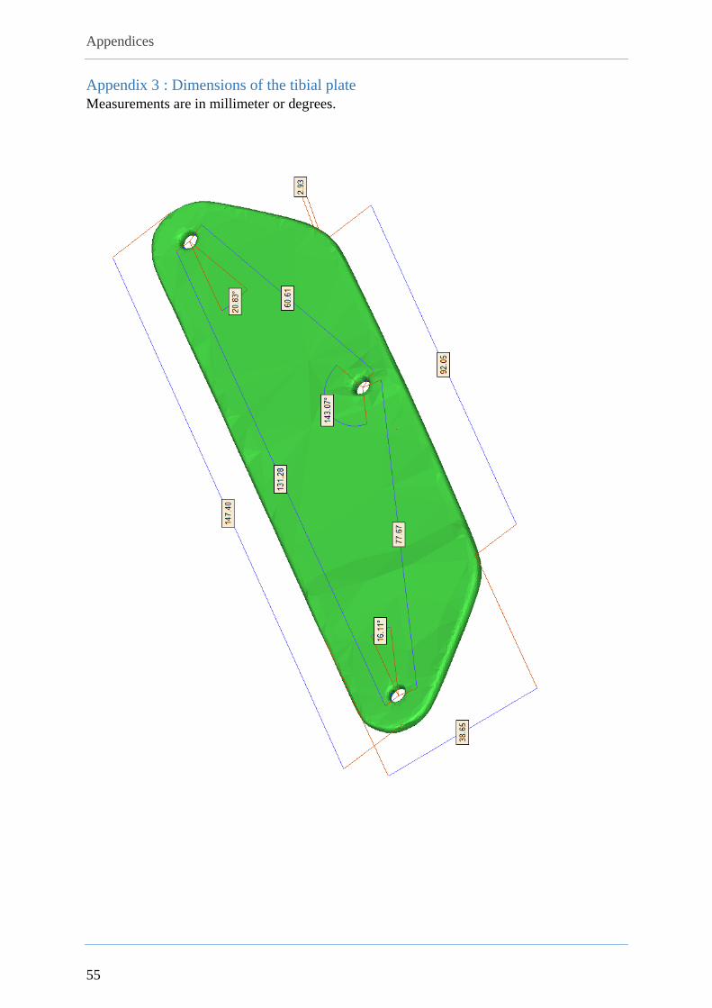
Appendices
55
Appendix 3 : Dimensions of the tibial plate
Measurements are in millimeter or degrees.

Appendices
56
Appendix 4 : Dimensions of the sacral plate
Measurements are in millimeter or degrees.

Appendices
57
Appendix 5 : Assessment of reliability of gait lab data
Both the reliability of gait data and CT image collection was estimated by repeated
measurements by different observers. The results were necessary to interpret forthcoming
results.
The reliability of the gait lab procedure, as outlined in 3.1.2, was rated by repeated gait
assessments on the same two subjects on four different days. Also, the assessments of the three
patients, included for this pilot study, before surgery was used. For every assessment the three-
dimensional coordinates of each marker (120 times per second) of one trial were exported to
the statistical software package of SPSS Statistics (v21.0 - © IBM, Armonk, New York, U.S.).
The three-dimensional position of the centre of gravity of each plate was determined (it was
believed that calculating the average x-, y- and z-coordinates for each three plate-markers was
sufficiently accurate as an estimation). The distances of these centres of gravity to various
points of interest were calculated and plotted in a line graph. Data was trimmed for extreme
values, such as sometimes occurred at the ends of the graphs (see Figure 11 below). These
extreme values mainly arose at the outside borders of the observed zone, mainly because of
reduced reliability in camera capture.
BEFORE AFTER
Figure 11: Example of how data was trimmed for extreme end values (graphs before and after trimming)
After trimming for these extreme values, the graphs had a cyclic pattern. Thus, most probably,
the remaining variation could be assigned to the gait pattern. The percent variation, defined by

Appendices
58
the range of this variation divided by the mean, was calculated for all the trials. On average,
this percent variation was 6.68% (minimum 3.79%, maximum 9.58%). This meant that a
similar effect-size (~6%) at least would be necessary to determine a significant difference
between e.g. pre- and post-surgery. Largest values of percent variation were found for the
distances from (1) sacral plate to the posterior iliac spine markers and (2) the tibial plates to
the calculated knee centres and tibial markers. Worth the thought could be that, although the
percent variation for the distance sacral plate-posterior iliac spines was the largest, its range
was not. Even more, with 8.06mm and 8.08mm, respectively to the left and right posterior iliac
spine, it was below the overall average range of 10.49mm. The surprising percent variation
could largely be due to its relative short distance from plate to marker (~4-6mm instead of e.g.
~24-26cm from tibial plate to ankle markers).
There were small differences to be noted between healthy subjects and knee OA patients, but
the average percent variation was nearly the same (6.68% versus 6.69%). Moreover, the
Wilcoxon matched-pair signed-ranks test was not significant, both for the range (p=0.124) as
well as the percent variation (p=0.363). Hence, it could be concluded that both (small) groups
were more or less comparable. More detail can be found in the table below.
Healthy subjects Knee OA patients Total
From To Range
(mm) Percent
variation Range
(mm) Percent
variation Range
(mm) Percent
variation
Sacral plate
LFEP 7.51 3.36% 14.40 5.61% 9.81 4.11%
RFEP 7.06 3.17% 11.27 4.37% 8.46 3.57%
LPSI 9.85 14.42% 4.49 8.18% 8.06 12.34%
RPSI 9.81 13.64% 4.61 7.93% 8.08 11.74%
LASI 10.44 4.35% 16.07 5.59% 12.32 4.76%
RASI 10.57 4.46% 12.68 4.38% 11.27 4.43%
Left tibial
plate
LFEO 12.36 6.48% 15.21 7.94% 13.31 6.97%
LKNE 9.55 5.01% 11.31 5.77% 10.13 5.27%
LTIB 9.24 8.76% 7.05 6.56% 8.51 8.02%
LANK 8.77 3.78% 10.73 5.78% 9.42 4.44%
Right tibial
plate
RFEO 17.22 10.06% 20.23 10.97% 18.22 10.36%
RKNE 8.86 5.13% 12.48 6.59% 10.06 5.62%
RTIB 8.15 6.74% 8.48 7.11% 8.26 6.86%
RANK 9.47 4.14% 13.82 6.89% 10.92 5.06%
AVERAGE (average - SD,
average + SD) 9.92 (7.43,
12.40)
6.68%
(2.98%,
10.38%)
11.63
(7.22,
16.04)
6.69%
(4.97%,
8.42%)
10.49
(7.74,
13.24)
6.68%
(3.79%,
9.58%) Table 14: Percent variation of gait analysis in healthy subjects and knee OA patients

Appendices
59
In the same way, also the reliability of the analysis in 3-matic was estimated. In total, two
observers each individually did 6 measurements on the same 3D surface objects (those of the
first patient included). The inter- and intra-observer reliability was defined by the average
distances in space the calculated points varied across the different analyses. The overall average
distance of variation was 2.22 mm. This distance was slightly larger between observers
(2.56mm) than intra-observer (2.07mm). Variation was highest in the pelvic area (LPSI, RPSI,
LASI and RASI). The different distances of variation for the plates, pelvic -, femoral - and
lower leg region can be found in the figure below.
Figure 12: Inter- and intra-observer variation in analysis in 3-matic
Comparison of the observations made by the two observers was done using a mixed-design
ANOVA. Mauchly’s Test of Sphericity did not allow to accept the condition of sphericity
(p<0.001). This meant that the variances of the various measurements of the anatomical
landmarks were significantly different. Subsequently, the Greenhouse-Geiser Correction
TOTAL:
0,90 1,08
3,61 4,97
2,13 2,20
2,54 3,37
2,07 2,56
Inter-observer variation
Intra-observer variation

Appendices
60
(ε=0.049) had to be used5, which increased the p-value from p<0.001 to p=0.074 for the
combined effect of anatomical landmark and observer. The p-value of the error that was
dependent on the landmark stayed smaller than 0.001. Already here, it could be assumed that
the landmark itself introduced more error than the person who made the observation.
Although the Levene’s Test of Equality of Error Variances was highly significant (p<0.001)
for eight of the 87 coordinates (three dimensions for 29 landmarks), the overall F-ratio was
2.628. Using the Test of Between-Subject Effects this corresponded to a p-value of 0.136. Thus,
the null hypothesis (there is no significant effect of rater) could be accepted.
Mauchly’s Test of Sphericity
Within Subjects Effect Mauchly's Test
Epsilon
(Greenhouse-
Geisser)
Anatomical landmark p<0.001 0.049
Tests of Within-Subjects Effects
Source F-ratio Significance
Anatomical landmark Sphericity Assumed 1115309.094 p<0.001
Greenhouse-Geisser 1115309.094 p<0.001
Anatomical landmark *
Observer
Sphericity Assumed 2.276 p<0.001
Greenhouse-Geisser 2.276 p=0.074
Table 15: Mixed-design ANOVA to test the effect of the observer on the measurements done in 3-matic
5 The Greenhouse-Geiser Correction should be used when ε < 0.75. Otherwise, the Huynh-Feldt Correction is
more appropriate. These correction factors reduce the number of degrees of freedom. In this way, the F-ratio’s are
made more conservative, which means they have to be larger to be as significant.

Appendices
61
Appendix 6 : Kinematic graphs comparing the Plug-in-Gait with the replica model
Gait cycle in x-axis, joint angles in degrees in y-axis. Normal values in gray.
BMJ pre-surgery PIG vs. PIGr
Generic Plug-in-Gait
model
Generic Plug-in-Gait
replica model
Left Left
Right Right
Current vrs Previous
Lef t Current (23-08-2013 PIG) Right Current (23-08-2013 PIG) Lef t 470524 070A38 PIGr.pxd (23-08-2013 PIGr) Right 470524 070A38 PIGr.pxd (23-08-2013 PIGr)
Pelvic Tilt30
-30
Ant
Post
deg
Hip Flexion/Extension60
-30
Flex
Ext
deg
Knee Flexion/Extension80
-10
Flex
Ext
deg
Ankle Dorsi/Plantar60
-60
Dors
Plan
deg
Pelvic Obliquity30
-30
Up
Down
deg
Hip Ab/Adduction30
-30
Add
Abd
deg
Knee Ab/Adduction30
-30
Var
Val
deg
Ankle Rotation70
-70
Int
Ext
deg
Pelvic Rotation30
-30
Int
Ext
deg
Hip Rotation40
-40
Int
Ext
deg
Knee Rotation30
-30
Int
Ext
deg
Foot Progress Angles60
-60
Int
Ext
deg

Appendices
62
BMJ post-surgery PIG vs. PIGr
Generic Plug-in-Gait
model
Generic Plug-in-Gait
replica model
Left Left
Right Right
Current vrs Previous
Lef t Current (28-02-2014 PIG) Right Current (28-02-2014 PIG) Lef t 470524 070A38 Post PIGr.pxd (28-02-2014 PIGr) Right 470524 070A38 Post PIGr.pxd (28-02-2014 PIGr)
Pelvic Tilt30
-30
Ant
Post
deg
Hip Flexion/Extension60
-30
Flex
Ext
deg
Knee Flexion/Extension80
-10
Flex
Ext
deg
Ankle Dorsi/Plantar60
-60
Dors
Plan
deg
Pelvic Obliquity30
-30
Up
Down
deg
Hip Ab/Adduction30
-30
Add
Abd
deg
Knee Ab/Adduction30
-30
Var
Val
deg
Ankle Rotation70
-70
Int
Ext
deg
Pelvic Rotation30
-30
Int
Ext
deg
Hip Rotation40
-40
Int
Ext
deg
Knee Rotation30
-30
Int
Ext
deg
Foot Progress Angles60
-60
Int
Ext
deg

Appendices
63
DBM pre-surgery PIG vs. PIGr
Generic Plug-in-Gait
model
Generic Plug-in-Gait
replica model
Left Left
Right Right
Current vrs Previous
Lef t 400914 034A61 18-10-2013 PIG.pxd (18-10-2013 PIG) Right 400914 034A61 18-10-2013 PIG.pxd (18-10-2013 PIG) Lef t 400914 034A61 18-10-2013 PIGr.pxd (18-10-2013 PIGr)
Right 400914 034A61 18-10-2013 PIGr.pxd (18-10-2013 PIGr)
Pelvic Tilt30
-30
Ant
Post
deg
Hip Flexion/Extension60
-30
Flex
Ext
deg
Knee Flexion/Extension80
-10
Flex
Ext
deg
Ankle Dorsi/Plantar60
-60
Dors
Plan
deg
Pelvic Obliquity30
-30
Up
Down
deg
Hip Ab/Adduction30
-30
Add
Abd
deg
Knee Ab/Adduction30
-30
Var
Val
deg
Ankle Rotation70
-70
Int
Ext
deg
Pelvic Rotation30
-30
Int
Ext
deg
Hip Rotation40
-40
Int
Ext
deg
Knee Rotation30
-30
Int
Ext
deg
Foot Progress Angles60
-60
Int
Ext
deg

Appendices
64
DBM post-surgery PIG vs. PIGr
Generic Plug-in-Gait
model
Generic Plug-in-Gait
replica model
Left Left
Right Right
Current vrs Previous
Lef t Current (07-03-2014 PIG) Right Current (07-03-2014 PIG) Lef t 400914 034A61 Post PIGr.pxd (07-03-2014 Post PIGr) Right 400914 034A61 Post PIGr.pxd (07-03-2014 Post PIGr)
Pelvic Tilt30
-30
Ant
Post
deg
Hip Flexion/Extension60
-30
Flex
Ext
deg
Knee Flexion/Extension80
-10
Flex
Ext
deg
Ankle Dorsi/Plantar60
-60
Dors
Plan
deg
Pelvic Obliquity30
-30
Up
Down
deg
Hip Ab/Adduction30
-30
Add
Abd
deg
Knee Ab/Adduction30
-30
Var
Val
deg
Ankle Rotation70
-70
Int
Ext
deg
Pelvic Rotation30
-30
Int
Ext
deg
Hip Rotation40
-40
Int
Ext
deg
Knee Rotation30
-30
Int
Ext
deg
Foot Progress Angles60
-60
Int
Ext
deg

Appendices
65
DRM pre-surgery PIG vs. PIGr
Generic Plug-in-Gait
model
Generic Plug-in-Gait
replica model
Left Left
Right Right
Current vrs Previous
Lef t Current (03-05-2013 PIG) Right Current (03-05-2013 PIG) Lef t 420820 018A29 03-05-2013 PIGr.pxd (03-05-2013 PIGr) Right 420820 018A29 03-05-2013 PIGr.pxd (03-05-2013 PIGr)
Pelvic Tilt30
-30
Ant
Post
deg
Hip Flexion/Extension60
-30
Flex
Ext
deg
Knee Flexion/Extension80
-10
Flex
Ext
deg
Ankle Dorsi/Plantar60
-60
Dors
Plan
deg
Pelvic Obliquity30
-30
Up
Down
deg
Hip Ab/Adduction30
-30
Add
Abd
deg
Knee Ab/Adduction30
-30
Var
Val
deg
Ankle Rotation70
-70
Int
Ext
deg
Pelvic Rotation30
-30
Int
Ext
deg
Hip Rotation40
-40
Int
Ext
deg
Knee Rotation30
-30
Int
Ext
deg
Foot Progress Angles60
-60
Int
Ext
deg
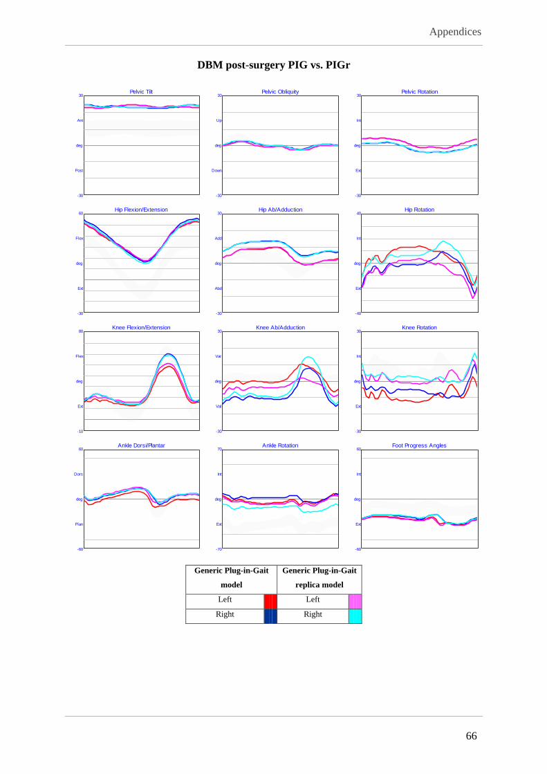
Appendices
66
DBM post-surgery PIG vs. PIGr
Generic Plug-in-Gait
model
Generic Plug-in-Gait
replica model
Left Left
Right Right
Current vrs Previous
Lef t Current (28-02-2014 PIG) Right Current (28-02-2014 PIG) Lef t 420820 018A29 Post PIGr.pxd (28-02-2014 PIGr) Right 420820 018A29 Post PIGr.pxd (28-02-2014 PIGr)
Pelvic Tilt30
-30
Ant
Post
deg
Hip Flexion/Extension60
-30
Flex
Ext
deg
Knee Flexion/Extension80
-10
Flex
Ext
deg
Ankle Dorsi/Plantar60
-60
Dors
Plan
deg
Pelvic Obliquity30
-30
Up
Down
deg
Hip Ab/Adduction30
-30
Add
Abd
deg
Knee Ab/Adduction30
-30
Var
Val
deg
Ankle Rotation70
-70
Int
Ext
deg
Pelvic Rotation30
-30
Int
Ext
deg
Hip Rotation40
-40
Int
Ext
deg
Knee Rotation30
-30
Int
Ext
deg
Foot Progress Angles60
-60
Int
Ext
deg

Appendices
67
Appendix 7 : Summary kinematic variables and their comparison between the generic PIG-model and the replica model PIG - PIGr Paired samples T-test Pearson correlation ICC (95% CI) F-test Mean Mean D SD (DIFF) 95% LOA
n=86 T-value p-value Correlation p-value Lower Upper p-value Lower Upper
Peak pelvic tilt (°) 0.244 0.808 0.984 <0.001 0.984 0.975 0.989 <0.001 18.871 0.022 0.834 -0.156 0.200
Range pelvic tilt (°) -2.191 <0.05 0.010 0.927 0.005 -0.194 0.207 0.481 3.192 -0.916 3.899 -1.747 -0.085
Peak pelvic obliquity (°) -2.176 <0.05 0.483 <0.001 0.450 0.268 0.602 <0.001 3.097 -0.511 2.190 -0.978 -0.044
Range pelvic obliquity (°) -2.473 <0.05 0.486 <0.001 0.459 0.276 0.609 <0.001 5.967 -0.617 2.328 -1.113 -0.121
Peak pelvic rotation (°) -1.543 0.127 0.161 0.136 0.074 -0.134 0.277 0.244 4.318 -2.260 13.661 -5.171 0.652
Range pelvic rotation (°) -1.831 0.071 -0.210 0.051 -0.047 -0.247 0.160 0.673 7.769 -3.258 16.597 -6.795 0.279
Peak hip flexion (°) 0.255 0.800 0.954 <0.001 0.954 0.931 0.970 <0.001 41.851 0.073 2.655 -0.496 0.642
Peak hip extension (°) 2.340 <0.05 0.983 <0.001 0.982 0.972 0.988 <0.001 4.384 0.410 1.624 0.062 0.758
Range hip flexion/extension (°) -1.453 0.150 0.937 <0.001 0.936 0.903 0.958 <0.001 37.467 -0.337 2.151 -0.798 0.124
Peak hip abduction (°) 0.677 0.500 0.984 <0.001 0.984 0.976 0.990 <0.001 -0.601 0.055 0.751 -0.106 0.216
Peak hip adduction (°) -1.415 0.161 0.973 <0.001 0.973 0.959 0.982 <0.001 9.184 -0.170 1.114 -0.409 0.069
Range hip abduction/adduction (°) -1.946 0.055 0.882 <0.001 0.878 0.818 0.919 <0.001 9.785 -0.225 1.071 -0.454 0.005
Peak hip external rotation (°) -0.162 0.871 0.917 <0.001 0.918 0.876 0.945 <0.001 -16.515 -0.086 4.890 -1.134 0.963
Peak hip internal rotation (°) 0.936 0.352 0.813 <0.001 0.809 0.722 0.871 <0.001 10.839 0.479 4.746 -0.538 1.497
Range hip rotation (°) 1.946 0.055 0.958 <0.001 0.956 0.933 0.971 <0.001 27.353 0.565 2.692 -0.012 1.142
Peak knee extension (°) -0.630 0.530 0.955 <0.001 0.954 0.930 0.970 <0.001 5.985 -0.140 2.057 -0.581 0.301
Range knee flexion extension (°) -2.827 <0.05 0.948 <0.001 0.944 0.911 0.964 <0.001 43.284 -0.769 2.522 -1.310 -0.228
Peak knee varus (°) 3.307 <0.05 0.870 <0.001 0.856 0.770 0.909 <0.001 9.923 1.387 3.889 0.553 2.221
Peak knee valgus (°) 3.600 <0.05 0.975 <0.001 0.971 0.949 0.983 <0.001 -6.105 0.614 1.581 0.275 0.953
Range knee varus/valgus (°) 2.260 <0.05 0.910 <0.001 0.891 0.835 0.928 <0.001 16.028 0.773 3.170 0.093 1.453
Peak knee external rotation (°) -0.835 0.406 0.025 0.818 0.022 -0.191 0.232 0.421 -7.283 -0.764 8.487 -2.583 1.056
Peak knee internal rotation (°) -0.977 0.332 0.683 <0.001 0.626 0.479 0.739 <0.001 9.551 -0.739 7.019 -2.244 0.766
Range knee rotation (°) 0.062 0.951 0.887 <0.001 0.888 0.834 0.926 <0.001 16.834 0.025 3.713 -0.771 0.821
Peak ankle plantarflexion (°) -5.984 <0.001 0.890 <0.001 0.780 0.522 0.885 <0.001 -8.291 -2.716 4.234 -3.618 -1.814
Range of dorsi/plantar flexion (°) 1.269 0.208 0.929 <0.001 0.928 0.893 0.953 <0.001 21.729 0.289 2.123 -0.164 0.741
Peak foot progression angle (°) -1.087 0.280 0.533 <0.001 0.437 0.251 0.592 <0.001 -9.836 -1.554 13.332 -4.396 1.287
Peak ankle external rotation (°) 1.863 0.066 0.674 <0.001 0.619 0.469 0.734 <0.001 -6.805 1.147 5.711 -0.077 2.372
Peak ankle internal rotation (°) -0.085 0.933 0.405 <0.001 0.385 0.188 0.552 <0.001 8.685 -0.084 9.187 -2.054 1.886
Range ankle rotation (°) -2.275 <0.05 0.226 <0.05 0.216 0.014 0.404 <0.05 15.490 -1.231 5.018 -2.307 -0.155
Peak knee flexion in swing (°) -2.679 <0.05 0.928 <0.001 0.923 0.880 0.951 <0.001 49.269 -0.909 3.146 -1.583 -0.234
Peak ankle dorsiflexion in swing (°) -4.726 <0.001 0.596 <0.001 0.485 0.249 0.654 <0.001 6.021 -2.190 4.323 -3.112 -1.269
Peak knee flexion in stance (°) -0.953 0.343 0.941 <0.001 0.937 0.906 0.959 <0.001 16.781 -0.285 2.770 -0.878 0.309
Peak ankle dorsiflexion in stance (°) -6.254 <0.001 0.588 <0.001 0.410 0.113 0.617 <0.001 13.476 -2.324 3.467 -3.063 -1.586
Ankle position at initial contact (°) -4.569 <0.001 0.468 <0.001 0.404 0.179 0.581 <0.001 1.711 -2.083 4.253 -2.990 -1.177
Mean -0.892 0.240 0.698 0.058 0.676 0.565 0.764 0.054 10.688 -0.539
0.883*
4.447 -1.490 0.412
Table 16: Summary kinematic variables and the comparison between the generic PIG-model and the replica model. ICC: intraclass correlation (two-way mixed effect, absolute agreement, single measures);
95% CI: 95% confidence interval; Mean D: average difference between the two models for the various assessments; SD (DIFF): standard deviation of the differences between the models; 95% LOA: 95%
limits-of-agreement (confidence interval for the mean differences); SEM: standard error of measurement; MDC: minimally detectable change; *average of the absolute values

Appendices
68
Appendix 8 : Kinematic graphs comparing the Plug-in-Gait with the CT-model
Gait cycle in x-axis, joint angles in degrees in y-axis. Normal values in gray.
BMJ pre-surgery PIG vs. CTM
CT-based subject-
specific model
Generic Plug-in-Gait
model
Left Left
Right Right
Current vrs Previous
Lef t 470524 070A38 CTM.pxd (23-08-2013 CTM) Right 470524 070A38 CTM.pxd (23-08-2013 CTM) Lef t 470524 070A38 PIG.pxd (23-08-2013 PIG)
Right 470524 070A38 PIG.pxd (23-08-2013 PIG)
Pelvic Tilt30
-30
Ant
Post
deg
Hip Flexion/Extension80
-31
Flex
Ext
deg
Knee Flexion/Extension80
-10
Flex
Ext
deg
Ankle Dorsi/Plantar60
-60
Dors
Plan
deg
Pelvic Obliquity30
-30
Up
Down
deg
Hip Ab/Adduction30
-30
Add
Abd
deg
Knee Ab/Adduction30
-30
Var
Val
deg
Ankle Rotation70
-70
Int
Ext
deg
Pelvic Rotation30
-30
Int
Ext
deg
Hip Rotation40
-40
Int
Ext
deg
Knee Rotation30
-30
Int
Ext
deg
Foot Progress Angles60
-60
Int
Ext
deg

Appendices
69
DBM pre-surgery PIG vs. CTM
CT-based subject-
specific model
Generic Plug-in-Gait
model
Left Left
Right Right
Current vrs Previous
Lef t Current (18-10-2013 CTM) Right Current (18-10-2013 CTM) Lef t 400914 034A61 18-10-2013 PIG.pxd (18-10-2013 PIG) Right 400914 034A61 18-10-2013 PIG.pxd (18-10-2013 PIG)
Pelvic Tilt30
-30
Ant
Post
deg
Hip Flexion/Extension60
-30
Flex
Ext
deg
Knee Flexion/Extension80
-10
Flex
Ext
deg
Ankle Dorsi/Plantar60
-60
Dors
Plan
deg
Pelvic Obliquity30
-30
Up
Down
deg
Hip Ab/Adduction30
-30
Add
Abd
deg
Knee Ab/Adduction30
-30
Var
Val
deg
Ankle Rotation70
-70
Int
Ext
deg
Pelvic Rotation30
-30
Int
Ext
deg
Hip Rotation40
-40
Int
Ext
deg
Knee Rotation30
-30
Int
Ext
deg
Foot Progress Angles60
-60
Int
Ext
deg

Appendices
70
DRM pre-surgery PIG vs. CTM
CT-based subject-
specific model
Generic Plug-in-Gait
model
Left Left
Right Right
Current vrs Previous
Lef t 420820 018A29_03-05-2013 CTM.pxd (03-05-2013 CTM) Right 420820 018A29_03-05-2013 CTM.pxd (03-05-2013 CTM) Lef t 420820 018A29_03-05-2013 PIG.pxd (03-05-2013 PIG)
Right 420820 018A29_03-05-2013 PIG.pxd (03-05-2013 PIG)
Pelvic Tilt40
-30
Ant
Post
deg
Hip Flexion/Extension74
-49
Flex
Ext
deg
Knee Flexion/Extension80
-10
Flex
Ext
deg
Ankle Dorsi/Plantar60
-60
Dors
Plan
deg
Pelvic Obliquity30
-30
Up
Down
deg
Hip Ab/Adduction30
-30
Add
Abd
deg
Knee Ab/Adduction30
-30
Var
Val
deg
Ankle Rotation70
-70
Int
Ext
deg
Pelvic Rotation30
-30
Int
Ext
deg
Hip Rotation40
-40
Int
Ext
deg
Knee Rotation60
-60
Int
Ext
deg
Foot Progress Angles60
-60
Int
Ext
deg

Appendices
71
Appendix 9 : Summary kinematic variables and the comparison between the PIG model and the CTM: Systematic differences by T-testing PIG - CTM (pre-surgery) BMJ (n=9) DBM (n=9) DRM (n=20) ALL (n=38)
Paired samples T-test Mean Mean D SD (of D) p-value Mean Mean D SD (of D) p-value Mean Mean D SD (of D) p-value Mean Mean D SD (of D) p-value
Peak pelvic tilt (°) 23.782 -12.982 1.180 <0.001 17.186 0.749 1.307 0.124 27.120 -12.688 2.973 <0.001 23.977 -9.575 6.261 <0.001
Range pelvic tilt (°) 5.137 -1.589 1.378 <0.05 2.638 -1.234 1.774 0.070 6.285 -7.458 2.984 <0.001 5.149 -4.594 3.878 <0.001
Peak pelvic obliquity (°) 3.614 0.322 8.602 0.913 1.297 0.148 2.763 0.877 1.705 0.613 3.111 0.389 2.060 0.434 4.760 0.578
Range pelvic obliquity (°) 4.214 5.226 1.002 <0.001 2.829 -0.218 1.391 0.651 3.280 0.936 1.577 <0.05 3.394 1.679 2.479 <0.001
Peak pelvic rotation (°) 3.548 0.674 4.912 0.691 1.632 -1.016 1.394 0.060 3.424 0.191 2.027 0.678 3.029 0.020 2.851 0.966
Range pelvic rotation (°) 6.436 -1.760 1.102 <0.05 3.517 -1.837 1.272 <0.05 6.972 0.171 1.100 0.494 6.027 -0.762 1.493 <0.05
Peak hip flexion (°) 53.407 -21.414 2.070 <0.001 41.277 -6.891 4.988 <0.05 51.971 -34.997 7.470 <0.001 49.778 -25.123 13.109 <0.001
Peak hip extension (°) 10.464 -18.198 3.777 <0.001 8.850 -4.093 1.727 <0.001 19.387 -26.558 8.158 <0.001 14.778 -19.257 11.087 <0.001
Range hip flexion/extension (°) 42.943 -3.217 3.712 <0.05 32.427 -2.798 4.314 0.088 32.584 -8.439 4.782 <0.001 35.000 -5.866 5.131 <0.001
Peak hip abduction (°) 0.384 4.901 11.532 0.238 -2.352 0.564 1.600 0.321 -3.641 2.655 3.125 <0.05 -2.383 2.692 6.051 <0.05
Peak hip adduction (°) 10.750 5.758 11.621 0.175 5.201 -0.657 1.040 0.095 4.641 0.466 3.942 0.604 6.220 1.453 6.598 0.183
Range hip abduction/adduction (°) 10.366 0.857 2.177 0.272 7.553 -1.221 1.613 0.053 8.282 -2.189 2.249 <0.001 8.603 -1.238 2.396 <0.05
Peak hip external rotation (°) -11.689 -15.624 4.983 <0.001 -0.565 -3.497 3.431 <0.05 -4.045 -22.561 14.372 <0.001 -5.031 -16.403 13.234 <0.001
Peak hip internal rotation (°) 9.702 -11.176 5.347 <0.001 14.236 -2.074 1.863 <0.05 13.151 -17.622 14.264 <0.001 12.591 -12.413 12.347 <0.001
Range hip rotation (°) 21.391 4.449 3.497 <0.05 14.801 1.422 4.447 0.365 17.197 4.939 4.133 <0.001 17.623 3.990 4.223 <0.001
Peak knee extension (°) 9.008 -4.252 2.970 <0.05 8.885 -4.710 6.271 0.054 6.028 -9.684 40.550 0.299 7.411 -7.219 29.355 0.138
Range knee flexion extension (°) 47.474 -12.388 3.398 <0.001 45.997 -7.838 3.938 <0.001 40.307 -7.434 7.222 <0.001 43.352 -8.703 6.082 <0.001
Peak knee varus (°) 6.017 -8.773 4.634 <0.001 13.456 3.792 2.564 <0.05 10.779 -9.300 5.476 <0.001 10.285 -6.074 7.248 <0.001
Peak knee valgus (°) -6.632 -12.483 5.441 <0.001 1.395 -1.561 3.225 0.184 2.173 -8.234 3.972 <0.001 -0.097 -7.660 5.625 <0.001
Range knee varus/valgus (°) 12.648 3.710 3.393 <0.05 12.061 5.353 1.628 <0.001 8.607 -1.066 3.279 0.162 10.382 1.586 4.115 <0.05
Peak knee external rotation (°) 8.628 -19.396 19.522 <0.05 -11.869 11.130 10.641 <0.05 -19.549 28.368 2.419 <0.001 -11.057 12.973 22.219 <0.001
Peak knee internal rotation (°) 19.099 -18.323 20.629 <0.05 -1.428 13.876 5.822 <0.001 -7.558 20.234 8.190 <0.001 0.208 9.596 19.723 <0.05
Range knee rotation (°) 10.472 1.072 4.109 0.456 10.442 2.746 5.183 0.151 11.991 -8.135 6.783 <0.001 11.264 -3.377 7.698 <0.05
Peak ankle plantarflexion (°) -0.104 -2.083 5.733 0.307 -6.909 1.668 6.489 0.463 -0.925 -4.979 18.621 0.246 -2.148 -2.719 14.206 0.246
Range of dorsi/plantar flexion (°) 16.618 -0.891 3.187 0.426 22.326 -1.768 5.309 0.347 18.488 0.034 4.853 0.976 18.954 -0.612 4.578 0.415
Peak foot progression angle (°) 0.217 -1.496 3.675 0.257 -9.219 1.439 1.700 <0.05 -19.629 0.521 7.398 0.756 -12.463 0.261 5.725 0.780
Peak ankle external rotation (°) -16.071 23.063 18.964 <0.05 3.257 -7.164 6.317 <0.05 -2.189 -6.841 10.977 <0.05 -4.187 0.165 17.759 0.955
Peak ankle internal rotation (°) -1.260 24.660 15.705 <0.05 14.801 -12.509 8.005 <0.05 12.356 -5.265 12.329 0.071 9.710 0.107 18.606 0.972
Range ankle rotation (°) 14.811 1.597 4.623 0.330 11.544 -5.344 4.768 <0.05 14.544 1.577 3.222 <0.05 13.897 -0.058 4.876 0.942
Peak knee flexion in swing (°) 56.482 -16.640 2.361 <0.001 54.882 -12.548 7.266 <0.001 46.335 -17.118 46.767 0.118 50.763 -15.922 33.755 <0.05
Peak ankle dorsiflexion in swing (°) 11.749 -1.471 5.226 0.423 3.958 1.179 3.714 0.369 9.842 -4.119 14.731 0.226 8.900 -2.237 11.190 0.226
Peak knee flexion in stance (°) 24.239 -9.323 2.169 <0.001 16.896 -5.142 5.765 <0.05 13.802 -9.572 41.272 0.313 17.007 -8.464 29.773 0.088
Peak ankle dorsiflexion in stance (°) 16.514 -2.974 7.283 0.255 15.417 -0.100 2.012 0.885 17.549 -4.917 14.204 0.138 16.799 -3.316 10.949 0.070
Ankle position at initial contact (°) 5.963 0.976 5.301 0.596 -0.462 3.399 3.445 <0.05 2.033 -2.797 17.376 0.480 2.373 -0.436 13.067 0.838
Mean -3.506 6.036 0.160 -1.081 3.794 0.156 -5.037 10.174 0.177 -3.737 10.660 0.219
Mean of the absolute values 8.051 3.873 8.608 5.794
Table 17: Summary kinematic variables and the comparison between the generic PIG-model and the CT-based subject-specific model (CTM): Systematic differences by means of T-testing. Mean D: average
difference between the two models (PIG-CTM); SD (of D): standard deviation of the differences between the models; p-value for the paired samples T-test (PIG-CTM)

Appendices
72
Appendix 10 : Summary kinematic variables and the comparison between the PIG model and the CTM: Correlation and agreement testing PIG - CTM (pre-surgery) BMJ (n=9) DBM (n=9) DRM (n=20) ALL (n=38)
Correlation Pearson p-value ICC p-value Pearson p-value ICC p-value Pearson p-value ICC p-value Pearson p-value ICC p-value
Peak pelvic tilt (°) -0.538 0.135 -0.003 0.936 0.701 <0.05 0.454 0.069 0.090 0.706 0.002 0.427 0.627 <0.001 0.113 <0.05
Range pelvic tilt (°) -0.265 0.491 -0.087 0.726 0.710 <0.05 0.375 0.095 0.109 0.646 0.010 0.390 0.064 0.703 0.016 0.411
Peak pelvic obliquity (°) -0.801 <0.05 -0.165 0.655 -0.676 <0.05 -0.647 0.946 0.902 <0.001 0.728 <0.001 0.506 <0.05 0.353 <0.05
Range pelvic obliquity (°) -0.573 0.107 -0.013 0.951 -0.564 0.113 -0.492 0.893 -0.320 0.168 -0.223 0.915 -0.674 <0.001 -0.318 1.000
Peak pelvic rotation (°) -0.855 <0.05 -1.031 0.999 0.204 0.599 0.142 0.299 0.962 <0.001 0.905 <0.001 0.727 <0.001 0.694 <0.001
Range pelvic rotation (°) 0.635 0.066 0.282 <0.05 0.238 0.537 0.085 0.274 0.688 <0.001 0.672 <0.001 0.767 <0.001 0.659 <0.001
Peak hip flexion (°) 0.780 <0.05 0.025 <0.05 -0.467 0.205 -0.126 0.908 -0.173 0.465 -0.003 0.624 -0.251 0.128 -0.029 0.823
Peak hip extension (°) 0.940 <0.001 0.146 <0.05 0.627 0.071 0.184 <0.05 0.125 0.600 0.006 0.383 0.284 0.084 0.044 0.171
Range hip flexion/extension (°) 0.629 0.070 0.411 0.056 -0.215 0.579 -0.139 0.700 0.458 <0.05 0.094 0.096 0.627 <0.001 0.424 <0.001
Peak hip abduction (°) -0.486 0.184 -0.061 0.571 -0.282 0.463 -0.270 0.779 0.896 <0.001 0.587 <0.001 0.379 <0.05 0.250 <0.05
Peak hip adduction (°) -0.933 <0.001 -0.410 0.926 -0.167 0.668 -0.124 0.677 0.838 <0.001 0.632 <0.05 0.253 0.126 0.235 0.072
Range hip abduction/adduction (°) 0.594 0.092 0.583 <0.05 -0.006 0.989 -0.004 0.506 -0.058 0.808 -0.029 0.597 0.338 <0.05 0.277 <0.05
Peak hip external rotation (°) 0.768 <0.05 0.142 <0.05 0.896 <0.05 0.772 <0.001 -0.267 0.255 -0.058 0.841 0.046 0.784 0.018 0.395
Peak hip internal rotation (°) 0.624 0.072 0.135 0.096 0.980 <0.001 0.958 <0.001 -0.751 <0.001 -0.209 1.000 -0.137 0.412 -0.064 0.797
Range hip rotation (°) -0.014 0.972 -0.005 0.515 0.520 0.151 0.400 0.127 0.647 <0.05 0.431 <0.001 0.634 <0.001 0.461 <0.001
Peak knee extension (°) 0.935 <0.001 0.824 <0.001 -0.871 <0.05 -0.381 0.983 0.259 0.271 0.083 0.359 0.239 0.148 0.102 0.263
Range knee flexion extension (°) 0.720 <0.05 0.153 <0.05 0.350 0.355 0.094 0.172 0.685 <0.001 0.457 <0.05 0.713 <0.001 0.395 <0.001
Peak knee varus (°) 0.378 0.316 0.055 0.284 0.970 <0.001 0.830 <0.001 0.216 0.360 0.067 0.173 0.327 <0.05 0.223 <0.05
Peak knee valgus (°) -0.761 <0.05 -0.070 0.982 0.648 0.059 0.116 0.362 0.674 <0.05 0.281 <0.001 0.536 <0.001 0.277 <0.001
Range knee varus/valgus (°) 0.378 0.316 0.225 0.141 0.973 <0.001 0.665 <0.001 0.006 0.980 0.004 0.493 0.532 <0.001 0.486 <0.001
Peak knee external rotation (°) -0.868 <0.05 -0.145 0.809 -0.449 0.225 -0.047 0.605 0.069 0.771 0.000 0.397 0.428 <0.05 0.076 0.277
Peak knee internal rotation (°) -0.633 0.067 -0.075 0.643 -0.344 0.364 -0.014 0.609 0.534 <0.05 0.053 0.107 0.694 <0.001 0.196 0.082
Range knee rotation (°) 0.595 0.091 0.473 0.089 -0.059 0.881 -0.029 0.538 0.421 0.064 0.126 0.131 -0.020 0.907 -0.012 0.533
Peak ankle plantarflexion (°) 0.834 <0.05 0.405 0.119 -0.285 0.457 -0.302 0.788 -0.190 0.423 -0.067 0.615 0.025 0.881 0.012 0.471
Range of dorsi/plantar flexion (°) 0.059 0.879 0.052 0.445 -0.152 0.696 -0.149 0.659 0.139 0.558 0.108 0.327 0.320 0.050 0.299 <0.05
Peak foot progression angle (°) 0.762 <0.05 0.642 <0.05 0.500 0.171 0.269 0.145 0.510 <0.05 0.176 0.231 0.849 <0.001 0.824 <0.001
Peak ankle external rotation (°) 0.957 <0.001 0.101 0.279 -0.071 0.855 -0.010 0.524 -0.740 <0.001 -0.457 1.000 0.060 0.721 0.035 0.419
Peak ankle internal rotation (°) 0.919 <0.001 0.161 0.131 0.118 0.762 0.036 0.381 -0.588 <0.05 -0.485 0.997 -0.068 0.684 -0.045 0.604
Range ankle rotation (°) -0.575 0.105 -0.563 0.957 0.405 0.279 0.158 0.211 0.279 0.234 0.219 0.138 0.047 0.779 0.048 0.388
Peak knee flexion in swing (°) 0.825 <0.05 0.085 <0.05 -0.070 0.859 -0.011 0.546 -0.273 0.244 -0.018 0.534 0.068 0.684 0.020 0.444
Peak ankle dorsiflexion in swing (°) 0.473 0.198 0.178 0.316 -0.651 0.058 -0.660 0.979 0.559 <0.05 0.140 0.267 0.468 <0.05 0.207 0.101
Peak knee flexion in stance (°) 0.909 <0.001 0.336 <0.001 -0.706 <0.05 -0.232 0.912 0.263 0.263 0.076 0.371 0.273 0.097 0.110 0.243
Peak ankle dorsiflexion in stance (°) 0.735 <0.05 0.306 0.186 0.332 0.383 0.274 0.242 0.054 0.822 0.024 0.456 0.133 0.427 0.059 0.353
Ankle position at initial contact (°) 0.221 0.568 0.200 0.302 0.225 0.561 0.113 0.298 0.059 0.805 0.017 0.471 0.120 0.472 0.064 0.353
Mean 0.217 0.143 0.097 0.361 0.099 0.338 0.067 0.449 0.208 0.281 0.128 0.363 0.292 0.241 0.191 0.246
Table 18: Summary kinematic variables and the comparison between the generic PIG-model and the CT-based subject-specific model (CTM): Correlation and agreement testing. Pearson: Pearson
correlation coefficient; ICC: intraclass correlation coefficient (ICC(3,1): two-way mixed effect, absolute agreement, single measures

Appendices
73
Appendix 11 : Temporal parameters pre- and post-surgery
Temporal parameters BMJ DBM DRM ALL
PRE-POST Mean Mean D T-test Mean Mean D T-test Mean Mean D T-test Mean Mean D T-test
PIG
Cadence L 101.225 11.994 <0.001 118.550 -12.700 <0.001 96.945 -38.310 <0.001 106.369 -15.158 <0.001
Cadence R 101.142 11.383 <0.001 118.300 -11.400 <0.001 96.635 -36.130 <0.001 106.774 -17.186 <0.001
Step length L 0.451 0.037 0.583 0.500 -0.074 <0.001 0.418 -0.165 <0.001 0.459 -0.075 <0.05
Step length R 0.459 -0.018 0.081 0.503 -0.101 <0.001 0.417 -0.153 <0.001 0.461 -0.105 <0.001
Step width L 0.165 -0.041 <0.001 0.132 0.001 0.843 0.213 0.029 <0.001 0.170 -0.001 0.902
Step width R 0.167 -0.037 <0.001 0.136 0.007 0.311 0.216 0.036 <0.001 0.173 0.009 0.426
Stride length L 0.882 -0.038 <0.001 0.998 -0.185 <0.001 0.837 -0.312 <0.001 0.910 -0.190 <0.001
Stride length R 0.887 -0.021 <0.05 1.002 -0.175 <0.001 0.836 -0.318 <0.001 0.916 -0.204 <0.001
Walking speed L 0.744 0.057 <0.001 0.990 -0.287 <0.001 0.701 -0.516 <0.001 0.822 -0.276 <0.001
Walking speed L 0.746 0.072 <0.05 0.994 -0.268 <0.001 0.696 -0.510 <0.001 0.833 -0.304 <0.001
CTM
Cadence L 101.433 10.467 <0.05 119.583 -13.167 <0.001 97.068 -36.436 <0.001 106.204 -19.166 <0.001
Cadence R 100.613 8.775 <0.05 119.325 -12.150 <0.001 97.269 -36.263 <0.001 103.812 -19.362 <0.001
Step length L 0.430 -0.020 0.086 0.503 -0.078 <0.001 0.422 -0.150 <0.001 0.452 -0.102 <0.001
Step length R 0.459 -0.008 0.580 0.502 -0.124 <0.001 0.428 -0.159 <0.001 0.457 -0.117 <0.001
Step width L 0.164 -0.038 <0.05 0.130 0.008 0.360 0.213 0.026 <0.05 0.173 0.007 0.620
Step width R 0.161 -0.033 <0.05 0.136 -0.001 0.905 0.219 0.030 <0.05 0.180 0.015 0.339
Stride length L 0.884 -0.018 0.266 1.002 -0.187 <0.001 0.849 -0.297 <0.001 0.912 -0.204 <0.001
Stride length R 0.881 -0.043 <0.05 1.001 -0.211 <0.001 0.839 -0.314 <0.001 0.894 -0.229 <0.001
Walking speed L 0.748 0.062 <0.05 1.003 -0.294 <0.001 0.708 -0.496 <0.001 0.824 -0.319 <0.001
Walking speed L 0.739 0.033 0.132 1.001 -0.307 <0.001 0.704 -0.511 <0.001 0.793 -0.336 <0.001
Table 19: Temporal parameters before and after surgery compared by means of T-testing. PIG: generic Plug-in-Gait model; CTM: CT-based subject-specific model; Mean: average of pre- and post-
surgical values; Mean D: average difference between pre- and post-surgical values; T-test: p-values for the independent T-test; Cadence in steps/min, step length and width and stride length in metres,
walking speed in metres/second

Appendices
74
Appendix 12 : Summary kinematic variables and the comparison between pre- and post-surgically: Systematic differences by T-testing
PRE-POST BMJ DBM DRM ALL
Paired samples T-test Bad side - R Good side Bad side - R Good side Bad side - L Good side Bad side Good side
p-values PIG CTM PIG CTM PIG CTM PIG CTM PIG CTM PIG CTM PIG CTM PIG CTM
Peak hip flexion (°) <0.001 <0.05 <0.001 <0.001 0.083 <0.001 <0.001 <0.05 <0.001 <0.001 <0.001 <0.001 <0.05 <0.05 <0.05 <0.05
Peak hip extension (°) <0.05 <0.05 <0.001 0.174 <0.001 0.824 <0.001 <0.001 <0.001 <0.001 <0.001 <0.001 0.319 <0.001 0.446 <0.001
Range hip flexion/extension (°) 0.729 <0.05 <0.05 <0.001 <0.001 <0.001 <0.001 <0.001 <0.001 <0.05 <0.001 <0.05 <0.001 <0.001 <0.001 <0.001
Peak knee extension (°) <0.001 <0.05 <0.05 0.583 <0.001 <0.001 0.408 <0.001 <0.001 <0.001 <0.001 0.830 0.270 <0.05 0.001 0.824
Range knee flexion extension (°) <0.05 <0.05 <0.001 <0.001 <0.001 <0.05 <0.001 <0.001 <0.001 <0.001 <0.001 0.081 <0.05 <0.05 <0.001 <0.001
Peak knee flexion in swing (°) <0.001 <0.05 <0.05 <0.001 <0.05 <0.001 <0.001 <0.05 <0.001 <0.001 <0.001 0.644 <0.05 0.940 <0.001 0.330
Peak knee flexion in stance (°) <0.05 <0.05 <0.05 0.954 0.439 <0.001 <0.001 0.122 <0.001 <0.001 <0.001 0.459 0.243 <0.05 <0.001 0.413
PRE-POST BMJ DBM DRM ALL
Mean differences Bad side - R Good side Bad side - R Good side Bad side - L Good side Bad side Good side
PIG CTM PIG CTM PIG CTM PIG CTM PIG CTM PIG CTM PIG CTM PIG CTM
Peak hip flexion (°) 12.220 -5.023 8.480 -10.937 1.588 -12.861 -4.942 -4.653 -19.199 43.390 -23.625 44.686 -5.944 16.133 -7.115 12.431
Peak hip extension (°) 11.490 6.027 12.250 -1.655 7.972 0.314 6.710 4.893 -7.950 48.636 -11.448 51.733 2.464 25.249 2.421 20.878
Range hip flexion/extension (°) 0.730 -11.050 -3.770 -9.282 -6.385 -13.175 -11.653 -9.547 -11.249 -5.246 -12.177 -7.047 -8.407 -9.116 -9.536 -8.447
Peak knee extension (°) 9.553 4.067 3.988 -0.698 4.790 -6.789 -0.583 6.058 -4.751 17.209 -18.107 -5.722 1.588 8.044 -6.764 -2.272
Range knee flexion extension (°) 5.427 6.490 -6.710 -12.443 -9.360 -9.486 -9.818 -7.952 -6.069 -7.881 -6.297 -8.623 -7.091 -7.844 -7.944 -9.416
Peak knee flexion in swing (°) 14.980 10.557 -2.722 -13.142 -4.570 -16.275 -10.401 -1.893 -10.820 9.327 -24.404 -14.345 -5.504 0.200 -14.708 -11.689
Peak knee flexion in stance (°) 12.133 9.573 4.300 -0.060 -5.628 -10.739 -4.629 1.423 -6.279 15.116 -22.867 -20.976 -2.846 6.539 -9.755 -8.976
Table 20: Summary kinematic variables and the comparison between the pre- and post-surgical assessment and between the generic PIG-model and the CT-based subject-specific model (CTM): Systematic
differences by paired samples T-testing (pre-post).