indoor scene segmentation using a structured light sensorfergus/drafts/kinect_names.pdf ·...

Computer Science Technical Report TR2011-939, May 2011Courant Institute of Mathematical Science, New York University

Indoor Scene Segmentation using a Structured Light Sensor

Nathan Silberman and Rob FergusDept. of Computer Science, Courant Institute, New York University

{silberman,fergus}@cs.nyu.edu

Abstract

In this paper we explore how a structured light depthsensor, in the form of the Microsoft Kinect, can assist withindoor scene segmentation. We use a CRF-based model toevaluate a range of different representations for depth in-formation and propose a novel prior on 3D location. Weintroduce a new and challenging indoor scene dataset, com-plete with accurate depth maps and dense label coverage.Evaluating our model on this dataset reveals that the com-bination of depth and intensity images gives dramatic per-formance gains over intensity images alone. Our resultsclearly demonstrate the utility of structured light sensorsfor scene understanding.

1. IntroductionScene understanding is a problem of primary importance

in vision. However, the diversity of objects, lighting, view-points and occlusions in natural scenes makes it a highlychallenging task. Many current approaches address it asa multi-class segmentation problem where the goal is toprovide a dense label field over the image pixels. Exist-ing methods, such as the layered segmentation of Yanget al. [24], Layout-CRF of Shotton et al. [21], generativeprobabilistic models of Li et al. [16] and hierarchical CRFsof He and Zemel [8] show good performance on datasetssuch as MSRC [21] and PASCAL [5]. While outdoor scenesform the majority of these datasets, indoor scenes pose moreof a challenge for current vision methods. In this setting,large texture-less regions (walls, ceilings) occupy a signifi-cant fraction of the image and many indoor objects are eas-ily confused (e.g. sofa/bed and chair/table). Notably, cur-rent stereo methods for depth recovery do not perform wellin this environment.

In this paper we explore multi-class scene segmentationusing the Microsoft Kinect. This device uses structuredlight methods to give an accurate depth map of the scene,which can be aligned spatially and temporally with the de-vice’s webcam (see Fig. 1). From a vision perspective,this device dramatically changes the scene understanding

(a) (b)

(d)(c)

Sofa SofaFloor

Picture Wall

Book-shelf

Blind

Figure 1. A typical indoor scene captured by the Microsoft Kinect.(a): Webcam image. (b) Raw depth map (red=close, blue=far). (c)Labels obtained via Amazon Mechanical Turk. (d) After a ho-mography, followed by pre-processing to fill in missing regions,the depth map (hue channel) can be seen to closely aligned withthe image (intensity channel). In this paper, we explore multi-classsegmentation using both image and depth, with the aid of manualannotations.

problem since depth is now an observed variable, as op-posed to one that must be inferred (typically with signifi-cant effort from incomplete information). Although struc-tured light methods for depth estimation have previouslybeen proposed [25], and other hardware methods measur-ing scene depth exist, e.g. LIDARs and time-of-flight cam-eras, the main attractions of the Kinect are that it is cheap,accurate, compact and portable (after a few modifications).These qualities make use of the device viable in numerousvision applications, such as assisting the visually impairedand robot navigation.

One clear limitation of the Kinect is that it can only op-erate reliably indoors, since the projected pattern is over-whelmed by exterior lighting conditions. We therefore fo-cus our attention on indoor scenes.

Recent work on indoor scene recognition by Hedauet al. [23] recovers the 3D structure of the room from asingle image, which then provides context for recognition.

1


In contrast, the explicit depth information provided by theKinect makes the recovery of the room geometry trivial.Other work that explicitly reasons about scene depth forrecognition includes: the scene context of Hoiem et al. [10],the hierarchical 3D scene model of Sudderth et al. [22], andstreet scene understanding using a car-mounted stereo rigby Leibe et al. [14].

In the robotics community, depth information is oftenavailable from LIDAR or stereo systems. Helmer and Loweexplore how stereo can aid recognition [9], while Gouldet al. combine laser range finder data with images [7]. Theclosest work to ours is that of Lai et al. [12] who also usea Kinect for recognition. Their use, however, is limited toisolated objects with uncluttered backgrounds, rather thanentire scenes, making their dataset qualitatively similar toCOIL [19].

This paper makes a number of contributions: (1) we in-troduce a new indoor scene dataset, of which every framehas an accurate depth map as well as a dense manually-provided labeling – to our knowledge, the first of its kind;(2) we describe simple modifications that make the Kinectfully portable, hence usable for indoor recognition; (3) weintroduce several new approaches that leverage the depthmap to give significant performance gains over image-basedmethods, validating the potential of the Kinect as a compo-nent in a recognition system.

2. ApproachBefore describing our multi-class segmentation model,

we first detail the hardware setup, data acquisition and pre-processing.

2.1. Capture Setup

The Kinect has two cameras: the first is a conventionalVGA resolution webcam that records color video at 30Hz.The second is an infra-red (IR) camera that records a non-visible structured light pattern generated by the Kinect’s IRprojector. The IR camera’s output is processed within theKinect to provide a smoothed VGA resolution depth map,also at 30Hz, with an effective range of ∼0.7–6 meters. SeeFig. 1(a) & (b) for typical output.

The Kinect requires a 12V input for the Peltier cooleron the IR depth camera, necessitating a mains adapter topower the device (USB sockets only provide 5V at limitedcurrents). Since the mains adapter severely limits portabil-ity of the device, we remove it and connect a rechargeable4200mAh 12V battery pack in its place. This is capable ofpowering the device for 12 hours of operation. The outputfrom the Kinect was logged on a laptop carried in a back-pack, using open-source Kinect drivers [18] to acquire timesynchronized image, depth and accelerometer feeds. Theoverall system is shown in Fig. 2(a). To avoid camera shakeand blur when capturing data, the Kinect was strapped to

a motion-damping rig built from metal piping, shown inFig. 2(b). The weights damp the motion and have a sig-nificant smoothing effect on the captured video.

Both the depth and image cameras on the Kinect werecalibrated using a set of checkerboard images in conjunc-tion with the calibration tool of Burrus [4]. This also pro-vided the homography between the two cameras, allowingus to obtain precise spatial alignment between the depth andRGB images, as demonstrated in Fig. 1(d).

Infra-RedLaser Projector

Depth Camera

RGB Webcam

Laptop

Microsoft Kinect

Mouse to (de)activate recording

BatteryPack

(a) (b)

Figure 2. (a): Our capture system with a Kinect modified to runfrom a battery pack. (b) Our capture platform, with counter-weights to damp camera movements.

2.2. Dataset CollectionWe visited a range of indoor locations within a large US

city, gathering video footage with our capture rig. Thesemainly consisted of residential apartments, having livingrooms, bedrooms, bathrooms and kitchens. We also cap-tured workplace and university campus settings. From theacquired video, we extracted frames every 2–3 seconds togive a dataset of 2151 unique frames, spread over 67 dif-ferent indoor environments. The dataset is summarized inTable 1. These frames were then uploaded to Amazon Me-chanical Turk and manually annotated using the LabelMeinterface [20]. The annotators were instructed to providedense labels that covered every pixel in the image (seeFig. 1(c)). Further details of the resulting label set are givenin Section 4.2.

2.3. Pre-processing

Following alignment with the RGB webcam images, thedepth maps still contain numerous artifacts. Most notable ofthese is a depth “shadow” on the left edges of objects. These

Scene class Scenes Frames Labeled FramesBathroom 6 2308 69Bedroom 19 18287 462Bookstore 2 27173 753Kitchen 11 11666 254

Living Room 14 14602 308Office 15 19254 305Total 67 93290 2151

Table 1. Statistics of captured sequences.

2


regions are visible from the depth camera, but not reachedby the infra-red laser projector pattern. Consequently theirdepth cannot be estimated, leaving a hole in the depth map.A similar issue arises with specular and low albedo surfaces.The internal depth estimation algorithm also produces nu-merous fleeting noise artifacts, particularly near edges.

Before extracting features for recognition, these artifactsmust be removed. To do this, we adapt the graph Laplacian-based colorization algorithm of Levin et al. [15]. Using theRGB image intensities, it guides the diffusion of the ob-served depth values into the missing shadow regions, re-specting the edges in intensity. An example result is shownin Fig. 1(d).

The Kinect contains a 3-axis accelerometer that allowsus to directly measure the gravity vector1 and hence esti-mate the pitch and roll for each frame. Fig. 3 shows the es-timate of the horizon for two examples. We rotate the RGBimage, depth map and labels to eliminate any pitch and roll,leaving the horizon horizontal and centered in the image.

Figure 3. Examples of images with significant pitch and rolloverlaid with horizon estimates, computed from the Kinect’s ac-celerometer.

3. ModelIn common with several other multi-class segmenta-

tion approaches [8, 21], we use a conditional random field(CRF) model as its flexibility makes it easy to explore a va-riety of different potential functions. A further benefit is thatinference can be performed efficiently with the graph-cutsoptimization scheme of Boykov et al. [2]2.

The CRF energy function E(y) measures the cost of alatent label yi over each pixel i in the image N . yi can takeon a discrete set of values {1, . . . , C}, C being the numberof classes. The energy is composed of three potential terms:(1) a unary cost function φ, which depends on the pixel lo-cation i, local descriptor xi and learned parameters θ; (2)a class transition cost ψ(yi, yj) between pairs of adjacentpixels i and j and (3) a spatial smoothness term η(i, j), alsobetween adjacent pixels, that varies across the image.

E(y) =∑i∈N

φ(xi, i|θ) +∑

i,j∈N

ψ(yi, yj)η(i, j) (1)

1During capture the device was moved slowly to minimize direct ac-celerations.

2In practice we use Bagon’s Matlab wrapper [1].

Before applying the CRF, we generate super-pixels{s1, . . . , sk} using the low-level segmentation approach ofFelzenszwalb and Huttenlocher [6]. We compute two dif-ferent sets of super-pixels: SRGB using the RGB image andSRGBD, which is computed using both RGB and depth im-ages3. We make use of super-pixels when computing theunary potentials φ, as explained in Section 3.1.1. We alsohave the option of using them in the spatial smoothness po-tential η (Section 3.3).

3.1. Unary Potentials

The unary potential function φ is the product of two com-ponents, a local appearance model and a location prior.

φ(xi, i|θ) = − log(P (yi|xi, θ)︸︷︷︸Appearance

P (yi, i)︸︷︷︸Location

) (2)

3.1.1 Appearance Model

Our appearance model P (yi|xi, θ) is discriminativelytrained using a range of different local descriptors xi, de-tailed below. For most of these, we use the same framework,which we now describe:

Given the set M of descriptors xm, computed over adense grid in all training images, we first learn a sparse cod-ing model [17]:

arg minαm,D

M∑m=1

‖xm −Dαm‖22 + λ‖αm‖1 s.t. αm > 0 (3)

where D is an |xm| × V codebook and αm are positivesparse code vectors of length V , where V = 1000 and λ =0.1. Note that during testing, only the sparse vectors αm areestimated, with the codebook D fixed.

Then, for each super-pixel sk within an image, we sumthe sparse vectors αi that fall within it. This gives super-pixel descriptors p̂k, which we normalize to sum to 1:

p̂k =∑i∈sk

αi, pk =p̂k∑p̂k

(4)

We now train a logistic regression model using pk fromall super-pixels in all training images. The model uses asoft-max output layer of dimension C, which is interpretedas P (yi|xi, θ). It has parameters θ (a weight matrix of size(V +1)×C) which are learned using back-propagation anda cross-entropy loss function. The ground truth labels y∗

for each super-pixel are taken from the dense image labelsobtained from Amazon Mechanical Turk.

Following training, the logistic regression model maps asuper-pixel descriptor pk directly to P (yi|xi, θ), which wecopy to all locations i within the super-pixel.

We use a range of different descriptor types as input xi

to the scheme above. In all cases, they are extracted overthe same dense grid4:

3Here, the input to [6] is the RGB image, with the blue channel replacedby an appropriately scaled depth map.

4Stride: 10 pixels; Patch size: 40× 40 pixels.

3


• RGB-SIFT: SIFT descriptors are extracted from theRGB image. This is our baseline approach.

• Depth-SIFT: SIFT descriptors are extracted from thedepth image. These capture both large magnitude gra-dients caused by depth discontinuities, as well as smallgradients that reveal surface orientation.

• Depth-SPIN: Spin image descriptors [11] are ex-tracted from the depth map. To review, this is a de-scriptor designed for matching 3D point clouds andsurfaces. Around each point in the depth image, a 2Dhistogram is built that counts nearby points as a func-tion of radius and depth. The histogram is vectorizedto form a descriptor.

We also propose several approach that combine informa-tion from the RGB and depth images:

• Joint-SIFT: SIFT descriptors are extracted from bothdepth and RGB images. At each location, the 128D de-scriptors both images are concatenated to form a single256D descriptor xi.

• Stacked-SIFT: SIFT descriptors are extracted fromboth depth and RGB images. Each are coded sepa-rately, giving two different pk’s for each super-pixel(pRGB

k and pDepthk ). These are concatenated to form a

2000D input to the logistic regression model.• Stacked-SPIN: Spin image descriptors are extracted

from the depth map, while SIFT is extracted from theRGB image. Each are coded separately and the re-sulting super-pixel descriptors concatenated to form a2000D input to the logistic regression model..

3.1.2 Location Prior

Our location prior P (yi, i) can take on two different forms.The first captures the 2D location of objects, similar to othercontext and segmentation approaches (e.g [21]). The sec-ond is a novel 3D location prior that leverages the depthinformation.

2D location priors: The 2D priors for each class arebuilt by averaging over every training image’s ground truthlabel map y∗. We then smooth the averaged map with an11 × 11 Gaussian filter. To compute the actual prior distri-bution P (yi, i), we normalize each map so it sums to 1/C,i.e.

∑i P (yi, i) = 1/C. Note that this assumes the prior

class distribution to be uniform5. Figure Fig. 4 shows theresulting distributions for 4 classes.

3D location priors: The depth information provided bythe Kinect allows us to estimate the 3D position of eachobject in the scene. However, the problem when buildinga prior is how to combine this information from scenes ofdiffering size and shape.

5In practice, if the true class frequencies are used, common classeswould be overly dominant in the CRF output.

Picture Bed Bookshelf Cabinet

Figure 4. 2D location priors for select object classes.

Our solution is to normalize the depth of an object, usingthe depth of the room itself. We assume that in any givencolumn6 of the depth map, the point furthest from the cam-era is on the bounding hull of the room. Fig. 5 demonstratesthe reliability of the procedure in separating the boundariesof the room from objects of similar depth. We scale thedepths of all points in a given column so that the furthestpoint has relative depth z̃ = 1. This effectively maps eachroom to a lie within a cylinder of radius 1.

Figure 5. A demonstration of our scheme for finding the bound-aries of the room. In this scene, the blue channel has been re-placed by a binary mask, set to 1 if the depth of point is within 4%of the maximum depth within each column (and 0 otherwise). Thewalls of the room are cleanly identified, while segmenting objectsof similar depth such as the fire extinguisher and towel dispenser.On the right, the cabinets and sink are correctly resolved as beingin the room interior, rather on the boundary.

Within this normalized reference frame, we can nowbuild histograms from the 3D positions of objects in thetraining set. Fig. 6 shows the relative depth histograms for4 different object classes, revealing distinctive profiles.

The actual priors are 3D histograms over (h, ω, z̃). h isthe absolute scene height relative to the horizon (in meters);ω is angle about the vertical axis and z̃ is relative depth. Inpractice, we find that many objects are near the boundary ofthe room, thus use a non-linear binning for z̃. Similar to the2D versions, the 3D histograms are normalized so that theysum to 1/C for each class (see Fig. 7 for examples).

6This is assisted by the pitch and roll correction made in pre-processing.

4


0.25 0.50 0.75 10

0.5

1

1.5

2

2.5

3

3.5

4

Relative Depth z

Prob

abili

ty D

ensi

ty

0.25 0.50 0.75 10

1

2

3

4

5

6

7

8

9

Relative Depth z

Prob

abili

ty D

ensi

ty

0.25 0.50 0.75 10

1

2

3

4

5

6

7

8

Relative Depth z

Prob

abili

ty D

ensi

ty

0.25 0.50 0.75 10

0.5

1

1.5

2

2.5

3

3.5

4

Relative Depth z

Prob

abili

ty D

ensi

ty

Table Television

WallBed

~ ~

~ ~

Figure 6. Relative depth histograms for table, television, bed andwall. As walls usually are on the boundary, they cluster near z̃ =1. Televisions lie just inside the room boundary, while tables andbeds are found in the room interior.

During testing, the extremal depth for each column in thedepth map is found and the relative 3D coordinate of eachpoint can be computed. Looking up these coordinates in the3D histograms gives the value of P (yi, i).

TableTelevision

ω

z = 0.21

Wall

~ z = 0.55~ z = 0.76 z = 0.87 z = 0.93 z = 0.98~ ~ ~ ~

-45 -450

0

(deg)

2

-1.5

h (m

eter

s)

Figure 7. 3D location priors for wall, television and table. Eachcolumn shows a different relative depth z̃. For each subplot, thex-axis is orientation ω about the vertical and the y-axis is heighth (relative to the horizon). The non-linear bin spacing in z̃ gives amore balanced distribution than linear spacing used in Fig. 6.

3.2. Class Transition Potentials

For this term we chose a simple Potts model [3]:

ψ(yi, yj) ={

0 if yi = yj

d otherwise (5)

The deliberate use of a simple class transition model allowsus to clearly see the benefits of the depth on the other twopotentials in the CRF. In our experiments we use d = 3.

3.3. Spatial Transition Potentials

The spatial transition cost η(i, j) provides a mechanismfor inhibiting or encouraging a label transition at each loca-tion (independently of the proposed label class). We exploreseveral options using a potential of the form:

η(i, j) = η0 e−α max(|I(i)−I(j)|−t,0) (6)

where |I(i) − I(j)| is gradient between adjacent pixels i, jin image I , t is a threshold and α and η0 are scaling factors.We use η0 = 100 for all the following methods:

• None: The baseline method is to keep η(i, j) = 0 forall i, j in the CRF. The smoothness of the labels y isthen solely induced by the class transition potential ψ.

• RGB Edges: We use IRGB in Eqn. 6, thus encouragingtransitions at intensity edges in the RGB image. α =40 and t = 0.04.

• Depth Edges: We use IDepth in Eqn. 6, with α = 30and t = 0.1. This encourages transitions at depth dis-continuities.

• RGB + Depth Edges: We combine edges from bothRGB and depth images, with η(i, j) = βηRGB(i, j) +(1− β)ηDepth(i, j) and β = 0.8.

• Super-Pixel Edges: We only allow transitions on theboundaries defined by the super-pixels, so set η(i, j) =0 on super-pixel boundaries and η0 elsewhere.

• Super-Pixel + RGB Edges: As for RGB-Edgesabove, but now we multiply |I(i) − I(j)| in Eqn. 6by the binary super-pixel boundary mask.

• Super-Pixel + Depth Edges: As for Depth-Edgesabove, but now we apply the binary super-pixel bound-ary mask to |I(i)− I(j)|.

4. ExperimentsBefore performing multi-class segmentation using our

CRF-based model, we first try the simpler task of scenerecognition to gauge the difficulty of our dataset.

4.1. Scene Classification

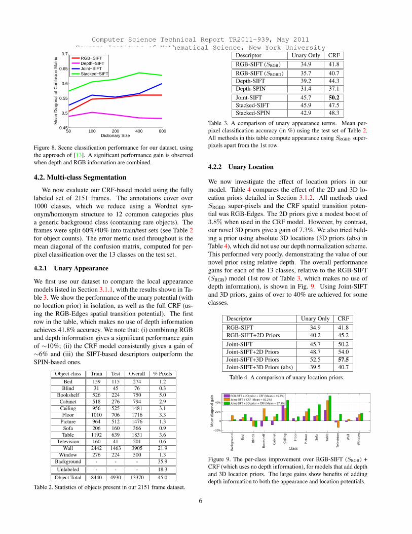
Table 1 shows the 6 scene-level classes in our dataset.We split each of these into disjoint sets of equal size, care-ful to ensure frames from the same scene are not in bothtrain and test sets. We apply the spatial pyramid matchingscheme of Lazebnik et al. [13], using SIFT extracted fromthe RGB image (standard features), as well as SIFT on thedepth image and both images (using the combination meth-ods explained in Section 3.1.1). The mean confusion matrixdiagonal is plotted in Fig. 8 as a function of k-means dictio-nary size for the different methods. Note that when usingthe RGB images, the accuracy is only 55%, far less than the81% achieved by the same method on the 15-class scenedataset used in [13]. This demonstrates the challenging na-ture of our data.

5


50 100 200 400 8000.45

0.5

0.55

0.6

0.65

0.7

Dictionary Size

Mea

n D

iago

nal o

f Con

fusi

on M

atrix

RGB−SIFTDepth−SIFTJoint−SIFTStacked−SIFT

Figure 8. Scene classification performance for our dataset, usingthe approach of [13]. A significant performance gain is observedwhen depth and RGB information are combined.

4.2. Multi-class Segmentation

We now evaluate our CRF-based model using the fullylabeled set of 2151 frames. The annotations cover over1000 classes, which we reduce using a Wordnet syn-onym/homonym structure to 12 common categories plusa generic background class (containing rare objects). Theframes were split 60%/40% into train/test sets (see Table 2for object counts). The error metric used throughout is themean diagonal of the confusion matrix, computed for per-pixel classification over the 13 classes on the test set.

4.2.1 Unary Appearance

We first use our dataset to compare the local appearancemodels listed in Section 3.1.1, with the results shown in Ta-ble 3. We show the performance of the unary potential (withno location prior) in isolation, as well as the full CRF (us-ing the RGB-Edges spatial transition potential). The firstrow in the table, which makes no use of depth informationachieves 41.8% accuracy. We note that: (i) combining RGBand depth information gives a significant performance gainof ∼10%; (ii) the CRF model consistently gives a gain of∼6% and (iii) the SIFT-based descriptors outperform theSPIN-based ones.

Object class Train Test Overall % PixelsBed 159 115 274 1.2

Blind 31 45 76 0.3Bookshelf 526 224 750 5.0

Cabinet 518 276 794 2.9Ceiling 956 525 1481 3.1Floor 1010 706 1716 3.3

Picture 964 512 1476 1.3Sofa 206 160 366 0.9Table 1192 639 1831 3.6

Television 160 41 201 0.6Wall 2442 1463 3905 21.9

Window 276 224 500 1.3Background - - - 35.9Unlabeled - - - 18.3

Object Total 8440 4930 13370 45.0

Table 2. Statistics of objects present in our 2151 frame dataset.

Descriptor Unary Only CRFRGB-SIFT (SRGB) 34.9 41.8RGB-SIFT (SRGBD) 35.7 40.7Depth-SIFT 39.2 44.3Depth-SPIN 31.4 37.1Joint-SIFT 45.7 50.2Stacked-SIFT 45.9 47.5Stacked-SPIN 42.9 48.3

Table 3. A comparison of unary appearance terms. Mean per-pixel classification accuracy (in %) using the test set of Table 2.All methods in this table compute appearance using SRGBD super-pixels apart from the 1st row.

4.2.2 Unary Location

We now investigate the effect of location priors in ourmodel. Table 4 compares the effect of the 2D and 3D lo-cation priors detailed in Section 3.1.2. All methods usedSRGBD super-pixels and the CRF spatial transition poten-tial was RGB-Edges. The 2D priors give a modest boost of3.8% when used in the CRF model. However, by contrast,our novel 3D priors give a gain of 7.3%. We also tried buld-ing a prior using absolute 3D locations (3D priors (abs) inTable 4), which did not use our depth normalization scheme.This performed very poorly, demonstrating the value of ournovel prior using relative depth. The overall performancegains for each of the 13 classes, relative to the RGB-SIFT(SRGB) model (1st row of Table 3, which makes no use ofdepth information), is shown in Fig. 9. Using Joint-SIFTand 3D priors, gains of over to 40% are achieved for someclasses.

Descriptor Unary Only CRFRGB-SIFT 34.9 41.8RGB-SIFT+2D Priors 40.2 45.2Joint-SIFT 45.7 50.2Joint-SIFT+2D Priors 48.7 54.0Joint-SIFT+3D Priors 52.5 57.5Joint-SIFT+3D Priors (abs) 39.5 40.7

Table 4. A comparison of unary location priors.

−20%

0

20%

40%

ClassBack

grou

nd

Bed

Blin

ds

Book

shel

f

Cabi

net

Ceili

ng

Floo

r

Pict

ure

Sofa

Tabl

e

Tele

visi

on

Wal

l

Win

dow

Mea

n di

agon

al g

ain

RGB-SIFT + 2D prior + CRF (Mean = 45.2%)Joint-SIFT + CRF (Mean = 50.2%)Joint-SIFT + 3D prior + CRF (Mean = 57.5%)

Figure 9. The per-class improvement over RGB-SIFT (SRGB) +CRF (which uses no depth information), for models that add depthand 3D location priors. The large gains show benefits of addingdepth information to both the appearance and location potentials.

6


In Fig. 10 we show three example images, each with la-bel maps output by 4 different models7. The baseline RGB-SIFT model (2nd row) makes mistakes which are implausi-ble based on the object location. Adding a 2D prior resolvesmany of these errors. The Joint-SIFT and 3D prior gives amore powerful spatial context, with the label map of the fi-nal model (5th row) being close to that of ground truth (6throw).

4.2.3 Spatial Transition PotentialsTable 5 explores different forms for the spatial transitionpotential. All methods use unary potentials based on SRGBDsuper-pixels and Joint-SIFT + 3D prior. The results showthat combining RGB and depth edges gives a performancegain of 5.6%. Using the super-pixel constraints does notgive a significant gain however.

Type CRFNone 53.4RGB Edges 57.5Depth Edges 56.6RGB + Depth Edges 59.0Super-Pixel Edges 55.7Super-Pixel + RGB Edges 56.4Super-Pixel + Depth Edges 52.7

Table 5. A comparison of spatial transition potentials. Mean per-pixel classification accuracy (in %).

5. DiscussionWe have introduced a new indoor scene dataset that com-

bines intensities, depth maps and dense labels. Using thisdata, our experiments clearly show that the depth informa-tion provided by the Kinect gives a significant performancegain over methods limited to intensity information. Thesegains have been achieved using a range of simple tech-niques, including novel 3D location priors. The magnitudeof the gains achieved makes a compelling case for the use ofdevices such as the Kinect for indoor scene understanding.

References[1] S. Bagon. Matlab wrapper for graph cut, December 2006. 3[2] Y. Boykov, O. Veksler, and R. Zabih. Efficient approx-

imate energy minimization via graph cuts. IEEE PAMI,20(12):1222–1239, 2001. 3

[3] Y. Boykov, O. Veksler, and R. Zabih. Fast approximate en-ergy minimization via graph cuts. IEEE PAMI, 23:1222–1239, 2001. 5

[4] N. Burrus. Kinect rgb demo v0.4.0. Website,2011. http://nicolas.burrus.name/index.php/Research/

KinectRgbDemoV2. 2[5] M. Everingham, L. Van Gool, C. K. I. Williams, J. Winn, and

A. Zisserman. The PASCAL Visual Object Classes Chal-lenge 2010. 1

7All use RGB-Edges for the spatial potential and SRGBD super-pixels

[6] P. Felzenszwalb and D. Huttenlocher. Efficient graph-basedimage segmentation. IJCV, 59(2), 2004. 3

[7] S. Gould, P. Baurnstark, M. Quigley, A. Ng, and D. Koller.Integrating visual and range data for robotic object detection.In ECCV Workshop (M2SFA2), 2008. 2

[8] X. He, R. Zemel, and M. Perpinan. Multiscale conditionalrandom fields for image labeling. In CVPR, 2004. 1, 3

[9] S. Helmer and D. G. Lowe. Using stereo for object recogni-tion. In ICRA, 2010. 2

[10] D. Hoiem, A. Efros, and M. Hebert. Putting objects in per-spective. IJCV, 80(1), October 2008. 2

[11] A. E. Johnson and M. Hebert. Using spin images for effi-cient object recognition in cluttered 3d scenes. IEEE PAMI,21(5):433–449, 1999. 4

[12] K. Lai, L. Bo, X. Ren, and D. Fox. A large-scale hierarchicalmulti-view rgb-d object dataset. In ICRA, 2011. 2

[13] S. Lazebnik, C. Schmid, and J. Ponce. Beyond bags offeatures: Spatial pyramid matching for recognizing naturalscene categories. In CVPR, 2006. 5, 6

[14] B. Leibe, N. Cornelis, K. Cornelis, and L. van Gool. Dy-namic 3D scene analysis from a moving vehicle. In CVPR,2007. 2

[15] A. Levin, D. Lischinski, and Y. Weiss. Colorization using op-timization. ACM Trans. Graph., Proc. SIGGRAPH, 23:689–694, 2004. 3

[16] L.-J. Li, R. Socher, and L. Fei-Fei. Towards total scene un-derstanding:classification, annotation and segmentation in anautomatic framework. In CVPR, 2009. 1

[17] J. Mairal, F. Bach, J. Ponce, and G. Sapiro. Online dictionarylearning for sparse coding. In ICML, 2009. 3

[18] H. Martin. Openkinect.org. Website, 2010. http://

openkinect.org/. 2[19] S. A. Nene, S. K. Nayar, and H. Murase. Columbia Object

Image Library (COIL-20). Technical report, Feb 1996. 2[20] B. C. Russell, A. Torralba, K. P. Murphy, and W. T. Free-

man. Labelme: A database and web-based tool for imageannotation. MIT AI Lab Memo, 2005. 2

[21] J. Shotton, J. Winn, C. Rother, and A. Criminisi. Texton-boost: Joint appearance, shape and context modeling formulti-class object recognition and segmentation. In ECCV,2006. 1, 3, 4

[22] E. Sudderth, A. Torralba, W. Freeman, and A. Willsky. Depthfrom familiar objects: A hierarchical model for 3d scenes. InCVPR, 2006. 2

[23] D. F. V. Hedau, D. Hoiem. Thinking inside the box: Usingappearance models and context based on room geometry. InECCV, 2010. 1

[24] Y. Yang, S. Hallman, D. Ramanan, and C. Fowlkes. Lay-ered object detection for multi-class segmentation. In CVPR,2010. 1

[25] L. Zhang, B. Curless, and S. Seitz. Rapid shape acquisi-tion using color structured light and multi-pass dynamic pro-gramming. In International Symposium on 3D Data Process-ing Visualization and Transmission, 2002. 1

7

http://nicolas.burrus.name/index.php/Research/KinectRgbDemoV2

http://nicolas.burrus.name/index.php/Research/KinectRgbDemoV2

http://openkinect.org/

http://openkinect.org/


Gro

und

trut

hJo

int-

SIFT

+ 3

D p

rior

Join

t-SI

FTRG

B-SI

FT +

2D

prio

rRG

B-SI

FTIm

age

Background Bed Blind Window Cabinet Ceiling

Picture Floor Sofa Table Television Wall

Figure 10. Three example scenes, along with outputs from 4 different models. See text for details. This figure is best viewed in color.

8

indoor scene segmentation using a structured light sensorfergus/drafts/kinect_names.pdf ·...

Documents