induced vibrations energy generation from vortex · pdf fileenergy generation from vortex...
TRANSCRIPT

ENERGY GENERATION FROM VORTEX INDUCED VIBRATIONS
BJS-VE10
A Major Qualifying Project
Submitted to the Faculty of the
WORCESTER POLYTECHNIC INSTITUTE
In partial fulfillment of the requirements for the
Degree of Bachelor of Science
By
Aaron Hall-Stinson
Christopher Lehrman
Everett Tripp
April 28, 2011
Submitted to Professor Brian J. Savilonis, Advisor
ii
Abstract
Vortex induced vibration is a well-known fluid flow phenomenon studied in multiple
engineering disciplines and typically sought to be minimized. However, a potential exists to
harness this phenomenon for electrical energy generation from low velocity marine currents. In
this project, a mathematical model was created to predict the dynamic response and
mechanical power of elastically mounted PVC cylinders subjected to a range of flow velocities.
Next, a six foot long open channel flow tank was designed and constructed to test cylinder
behavior over a range of flow velocities. A total of 85 tests were conducted using five different
cylinder diameters, each with several different masses, suspended on springs from a fixed
apparatus submerged in the channel. Cylinder displacement, velocity, and acceleration, as well
as flow velocity, were measured and recorded at a rate of 20 Hz over a one minute test interval
for each trial. From these data, oscillation frequency, mean amplitude, and fluid force vs. time
were calculated, as well as an estimate of available mechanical power in the cylinder
oscillations. These calculations were then used with other derived properties to develop a
single power coefficient curve over the range 5x10³< Re <1.5x10⁴. Additionally, efficiency
calculations indicated that the 0.75” cylinder had the most ideal aspect ratio of the cylinders
considered. In terms of power density, the 1” cylinder produced the maximum result of
10W/m3.

iii
Table of Contents
Abstract ............................................................................................................................................................................................................... ii
Table of Contents ............................................................................................................................................................................................ iii
Table of Figures .................................................................................................................................................................................................v
Table of Tables ............................................................................................................................................................................................... vii
1 Introduction ............................................................................................................................................................................................ 1
2 Background ............................................................................................................................................................................................. 3
2.1 VIV Theory .................................................................................................................................................................................... 3
2.1.1 Vortex Shedding .................................................................................................................................................................... 5
2.1.2 Strouhal Number .................................................................................................................................................................. 6
2.1.3 Lock In ....................................................................................................................................................................................... 7
2.1.4 Boundary Gap ...................................................................................................................................................................... 10
2.2 VIVACE.......................................................................................................................................................................................... 11
3 Modeling ................................................................................................................................................................................................. 12
4 Methodology ......................................................................................................................................................................................... 18
4.1 Experimental Setup ................................................................................................................................................................ 18
4.1.1 Materials ................................................................................................................................................................................. 19
4.1.2 Description ............................................................................................................................................................................ 19
4.2 Experimental Procedure ...................................................................................................................................................... 29
4.2.1 Data Collection ..................................................................................................................................................................... 29
4.2.2 Flow Profile Measurements ........................................................................................................................................... 31
4.2.3 Spring Stiffness .................................................................................................................................................................... 31
4.2.4 Cylinder Dimensions ......................................................................................................................................................... 31
4.2.5 Natural Frequency and Damping ................................................................................................................................ 32
4.2.6 Cylinder Displacement ..................................................................................................................................................... 33
5 Analysis and Results.......................................................................................................................................................................... 34
5.1 Data Analysis and Reduction Process ............................................................................................................................. 34
5.1.1 Still Water Decay Tests .................................................................................................................................................... 35

iv
5.1.1.1 Natural Frequency .................................................................................................................................................. 36
5.1.1.2 Damping Ratio .......................................................................................................................................................... 37
5.1.1.3 Hydrodynamic Mass ............................................................................................................................................... 38
5.1.2 Flowing Water Tests ......................................................................................................................................................... 39
5.1.2.1 Flow Speed ................................................................................................................................................................. 41
5.1.2.2 Oscillation Frequency ............................................................................................................................................ 41
5.1.2.3 Mean Amplitude ....................................................................................................................................................... 44
5.1.2.4 Potential Mechanical Power ............................................................................................................................... 45
5.2 Results & Discussion .............................................................................................................................................................. 46
5.2.1 Oscillation frequency ........................................................................................................................................................ 46
5.2.2 Power Coefficient ............................................................................................................................................................... 48
5.2.3 Power Harnessing Efficiency ........................................................................................................................................ 49
5.2.4 Damping ................................................................................................................................................................................. 50
5.2.5 Hydrodynamic Mass.......................................................................................................................................................... 51
5.2.6 Power Density ...................................................................................................................................................................... 52
5.2.7 Cylinder Amplitude ........................................................................................................................................................... 54
5.2.8 Observations......................................................................................................................................................................... 55
6 Recommendations for Future Work .......................................................................................................................................... 56
6.1 Project Continuation Proposal ........................................................................................................................................... 56
6.2 Task Specifications .................................................................................................................................................................. 57
6.3 Design Concepts ....................................................................................................................................................................... 61
6.4 Suggested Experiments ......................................................................................................................................................... 62
7 Conclusions ........................................................................................................................................................................................... 64
8 References ............................................................................................................................................................................................. 66
Appendix A Still Water Decay Test Data ...................................................................................................................................... 67
Appendix B Flowing Water Test Data ........................................................................................................................................... 68
v
Table of Figures
Figure 1: Vortex shedding Regimes (MIT) ........................................................................................................................................... 5
Figure 2: Strouhal Number vs. Reynolds number (MIT OCW) .................................................................................................... 7
Figure 3: Reduced Velocity vs. Mass Ratio (Williamson and Govardhan) ............................................................................. 9
Figure 4: Cylinder Amplitude over Diameter as a Function of Time ...................................................................................... 15
Figure 5: Derived Cylinder Velocity ...................................................................................................................................................... 16
Figure 6: Cylinder Power with Defining Parameters .................................................................................................................... 17
Figure 7: Tank and Channel Top View ................................................................................................................................................. 20
Figure 8: Tank and Channel Isometric View ..................................................................................................................................... 20
Figure 9: Pumps Top View ........................................................................................................................................................................ 21
Figure 10: Pumps Isometric View .......................................................................................................................................................... 21
Figure 11: Flow Guides Top View .......................................................................................................................................................... 22
Figure 12: Tank with Pumps and Flow Guides ................................................................................................................................ 22
Figure 13: Cylinder Diameters ................................................................................................................................................................ 23
Figure 14: Cylinder with Platform Apparatus .................................................................................................................................. 23
Figure 15: Cylinder Housing ..................................................................................................................................................................... 24
Figure 16: Cylinder Arrangement Front View .................................................................................................................................. 25
Figure 17: Cylinder Arrangement Isometric View ......................................................................................................................... 25
Figure 18: Cylinder Arrangement in Channel ................................................................................................................................... 26
Figure 19: Test Set Up ................................................................................................................................................................................. 27
Figure 20: Vernier MD BTD Sensor and Flow Rate Sensor ......................................................................................................... 27
Figure 21: Measurement Location Top View .................................................................................................................................... 28
Figure 22: Measurement Location Isometric View ........................................................................................................................ 28
Figure 23: Final Set-Up ............................................................................................................................................................................... 28
Figure 24: The LoggerPro Interface ...................................................................................................................................................... 30
Figure 25: Experimental Data Flowchart ........................................................................................................................................... 34
Figure 26: Free Decay Test Sample Trial ............................................................................................................................................ 36
Figure 27: flow speed time series from 1" cylinder ....................................................................................................................... 41
vi
Figure 28: MATLAB FFT Script ............................................................................................................................................................... 42
Figure 29: 1.0" Cylinder Single Sided Amplitude Spectrum ....................................................................................................... 43
Figure 30: 0.75" Cylinder Phase Portrait ............................................................................................................................................ 44
Figure 31: Non-Dimensional Frequency Results ............................................................................................................................ 47
Figure 32: Plot of Power Coefficients vs. Reynolds Number ...................................................................................................... 48
Figure 33: Power Efficiency vs. Reduced Velocity .......................................................................................................................... 49
Figure 34: Mechanical Power Component Terms........................................................................................................................... 50
Figure 35: Power Density Schematic .................................................................................................................................................... 52
Figure 36: Schematic of the Alden Labs Test Flume ...................................................................................................................... 57
Figure 37: Slider Concept Design ........................................................................................................................................................... 61
Figure 38: Right View of Slider Concept ............................................................................................................................................. 61

vii
List of Tables
Table 1: Cylinder and Flow Parameters .............................................................................................................................................. 12
Table 2: Cylinder Mass by Diameter ..................................................................................................................................................... 23
Table 3: Flow Profile Locations ............................................................................................................................................................... 31
Table 4: Damping Test Configurations ................................................................................................................................................ 32
Table 5: Cylinder Diameter-Mass Configurations Used in Experiments .............................................................................. 33
Table 6: Free Decay Test Summary Data ............................................................................................................................................ 35
Table 7: 0.75" Cylinder Trial 1Final Results ...................................................................................................................................... 39
Table 8: Power Density by Cylinder Diameter ................................................................................................................................. 53
Table 9: Proposed Setups for Testing the Lock-in Range ............................................................................................................ 63
Table 10: Data Summary of 0.75" Cylinder........................................................................................................................................ 67
Table 11: Data Summary of 1" Cylinder .............................................................................................................................................. 67
Table 12: Data Summary of 1.5" Cylinder .......................................................................................................................................... 67
Table 13: Data Summary of 2" Cylinder .............................................................................................................................................. 67
Tables 14: 0.75" Cylinder Final Data .................................................................................................................................................... 68
Tables 15: 1" Cylinder final Data ............................................................................................................................................................ 69
Tables 16: 1.5" Cylinder final Data ........................................................................................................................................................ 70
Tables 17: 2" Cylinder final Data ............................................................................................................................................................ 71

1
1 Introduction
The global demand for scalable renewable energy sources is large and ever growing.
Many hydrokinetic energy technologies exist currently, but are unable to truly meet this
demand due to self-limitations. The Earth’s water bodies constitute a huge portion of the
planet and their slow and steady motion represents a vast, but as yet untapped energy
resource. Most energy is currently harnessed from water flow by the joint effort of a dam and a
hydroelectric generator. Newer and less ecologically intrusive technology is needed to support
growing energy demand. One promising new technology that meets these criteria utilizes
vortex induced vibrations in water to extract energy.
Structures subjected to fluid flow are usually designed to minimize fatigue caused by
vortex induced vibrations. Only recently has the idea been proposed to enhance the vibrations
in order to maximize energy extraction from the fluid. This technology works by securing a
cylinder horizontally in water and constraining it to a single degree of freedom; movement up
and down in the plane perpendicular to the fluid flow. Flow over this cylinder creates an
alternating vortex pattern which exerts alternating lift forces on the cylinder, pushing it up and
down. This motion is then converted into electricity via a power take off mechanism.
This technology is superior to traditional hydro technology in several ways. Most turbine
based converters only operate efficiently at currents greater than 2 m/s, while surface
oscillation converters only give high output over a small range of wave frequencies. A vortex
induced vibration based generator could potentially function in slow moving waterways over a
wide range of frequencies. Further, Large scale tidal and dam type systems are very capital
intensive and environmentally obtrusive. The VIV concept is capable of producing energy from
water flow without altering the local environment, posing any danger to nearby residents,
changing the landscape in any visible way, or interfering with water traffic in any slow moving
waterway (0.5-5 knots).
Energy generation from VIV has significant potential for coastal areas as well. Fifty
percent of the U.S. population lives within 50 miles of the coast, whereas this coastal land
accounts for only 11 percent of U.S. territory. Energy demand in these coastal regions is
predictably larger than inland regions.

2
Scalability and versatility are two of the greatest strengths of this technology. Modules
can range in size from single cylinder arrays to mega-watt producing power plants. Areas of
potential power production include water bodies and/or rivers such as the Gulf Stream, the
Columbia, the Missouri, the Colorado, the Mississippi, the Kansas, and the Ohio. All water
bodies listed contain segments of flow averaging in the prime production speeds required for
this technology, which are significantly lower than other turbine based hydrokinetic
technologies.
This study examined the potential for vortex induced vibrations as a source of
energy by accomplishing the following goals:
• The development of a mathematical model to predict the dynamic response of a cylinder
in water flow
• The design of a small-scale setup and methodology to experimentally test cylinder
behavior under varying conditions
• The use of the experimental results to determine potential mechanical power and
efficiency, and the validity of the model
• The use of observations and data to propose a larger scale testing setup with power
take-off ability
3
2 Background
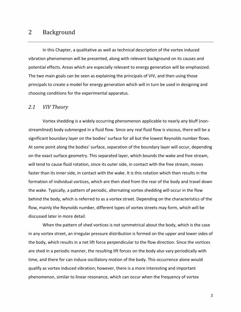
In this Chapter, a qualitative as well as technical description of the vortex induced
vibration phenomenon will be presented, along with relevant background on its causes and
potential effects. Areas which are especially relevant to energy generation will be emphasized.
The two main goals can be seen as explaining the principals of VIV, and then using those
principals to create a model for energy generation which will in turn be used in designing and
choosing conditions for the experimental apparatus.
2.1 VIV Theory
Vortex shedding is a widely occurring phenomenon applicable to nearly any bluff (non-
streamlined) body submerged in a fluid flow. Since any real fluid flow is viscous, there will be a
significant boundary layer on the bodies’ surface for all but the lowest Reynolds number flows.
At some point along the bodies’ surface, separation of the boundary layer will occur, depending
on the exact surface geometry. This separated layer, which bounds the wake and free stream,
will tend to cause fluid rotation, since its outer side, in contact with the free stream, moves
faster than its inner side, in contact with the wake. It is this rotation which then results in the
formation of individual vortices, which are then shed from the rear of the body and travel down
the wake. Typically, a pattern of periodic, alternating vortex shedding will occur in the flow
behind the body, which is referred to as a vortex street. Depending on the characteristics of the
flow, mainly the Reynolds number, different types of vortex streets may form, which will be
discussed later in more detail.
When the pattern of shed vortices is not symmetrical about the body, which is the case
in any vortex street, an irregular pressure distribution is formed on the upper and lower sides of
the body, which results in a net lift force perpendicular to the flow direction. Since the vortices
are shed in a periodic manner, the resulting lift forces on the body also vary periodically with
time, and there for can induce oscillatory motion of the body. This occurrence alone would
qualify as vortex induced vibration; however, there is a more interesting and important
phenomenon, similar to linear resonance, which can occur when the frequency of vortex
4
shedding fS is close to the natural frequency of the body in motion, fN. In this phenomenon,
referred to as “lock in”, the vortex shedding frequency actually shifts to match the bodies’
natural frequency, and as a result, much larger amplitudes of vibration can occur. It is this
particular aspect of vortex induced vibration, lock in, which has traditionally been of greatest
concern to structural engineers, since it poses the greatest risk of damage or failure.
Accordingly, the range of shedding frequencies which lock in can occur over is one of the most
important research areas within vortex induced vibration, and will be discussed in more depth
as it is also very relevant to the design of an energy harnessing device.
The phenomenon of vortex induced vibration is rather unique, as it is both widely
known and yet still poorly understood. Historical records show that vortex shedding had been
observed as early as the 15th century by da Vinci in the form of a vortex row forming behind a
piling submersed in a stream (Blevins). In perhaps the first scientific analysis, Strouhal found in
1878 that the Aeolian tones caused by a wire suspended in the wind were proportional to the
ratio of the wind speed to wire thickness (Blevins). In modern times, much research has been
undertaken to examine both the dynamics of vortex shedding, as well as the parameters which
most influence a bodies’ motion during vortex induced vibration. Although important, the
details of vortex shedding itself are not as relevant to energy extraction as the flow conditions
and body properties are. Therefore, more focus will be given to this later area.
From the description given earlier, it can be seen that many engineered structures
which are subjected to steady fluid flow may be susceptible to vortex induced vibration. A
broad range of applications, including, but certainly not limited to, offshore structures, marine
risers, heat transfer equipment, mooring cables, bridges and other civil structures, nuclear
reactor components, and cooling stacks are all areas where the possibility of VIV must be taken
into account during the design process. Accordingly, a vast majority of the past research has
focused on how to suppress vortex shedding and reduce the effects of VIV on structural
motion. Despite this, the information available is still quite useful in understanding the
phenomenon, and is still relevant to the topic of energy generation, where it is desired to
maximize, rather than suppress VIV. As a final comment, it should be noted that much of the
research encountered on VIV is still in the experimental and empirical areas, rather than
analytical, and as a result it can at best be used as a guideline in the design process.

5
2.1.1 Vortex Shedding
Like many fluid flow phenomenon, vortex shedding has been observed to be directly
dependent on the Reynolds number of the flow, which is defined in Eq. 2-1.
Eq. 2-1
U is the free stream velocity, D is the cylinder diameter, and is the kinematic viscosity of the
fluid. As a note, most studies in literature were in fact performed using a submerged cylinder,
which is the geometry later used in the experimental methodology, so the correlation length of
cylinder diameter used in Re is appropriate and widely applicable, as many submerged
structures are typically cylindrical in shape.
Figure 1: Vortex shedding Regimes (MIT)

6
The various vortex shedding patterns which occur over different ranges of Reynolds
number are presented in Figure 1. For the lowest two regimes, periodic vortex shedding is
nonexistent, and no resulting lift forces act on the body. For Re >40, a vortex street begins to
form, which does in fact result in varying lift forces, since the vortices shed non symmetrically
from the top and bottom of the cylinder. Between 150< Re<300-400, the first transition zone
occurs, in which the vortex street changes from laminar flow to turbulent. As a result, no
organized shedding or lift occurs in this region. For ~400<Re< 3x10⁵, the vortex street is fully
turbulent, and strong, periodic shedding results (Blevins, 1990). The second transition region
occurs when the flow around the cylinder changes from laminar to turbulent, and again vortex
shedding is disrupted and irregular. The agreed upon ranges for this transition region were
found to be varying, with the results of Lienhard giving 3x10⁵<Re< 3.5x10⁶ (Blevins), but
experimental measurements by Bernitsas give the range as 3x10⁵<Re< 5x10⁵. Above this final
transition region, from Re>5x10⁵ to 3.5x10⁶, both the vortex street and cylinder boundary layer
are turbulent, and regular vortex shedding resumes.
The ranges of no periodic vortex shedding, or dead zones (Bernitsas), must obviously be
avoided for any device extracting energy from VIV. For the experimental system described in
the methodology, the Reynolds number is on the order of the range 103<Re<104, which is well
clear of both the transition zones.
2.1.2 Strouhal Number
An additional non-dimensional parameter has been established to relate the frequency
of vortex shedding fS to the flow conditions. This is given by the Strouhal number S, and is
defined in Eq. 2-2.
Eq. 2-2
Again, U is the free stream velocity, and D is the cylinder diameter. For a wide range of
Reynolds number, the Strouhal number varies very little, and can essentially be taken as
constant, as seen in Figure 2.
7
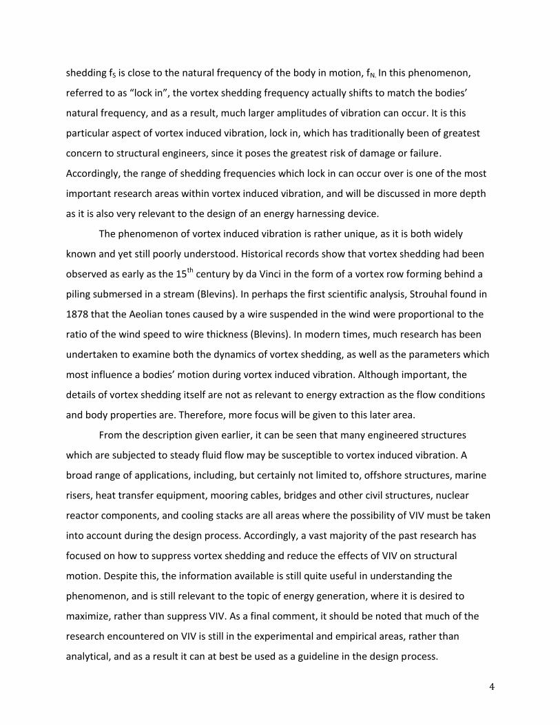
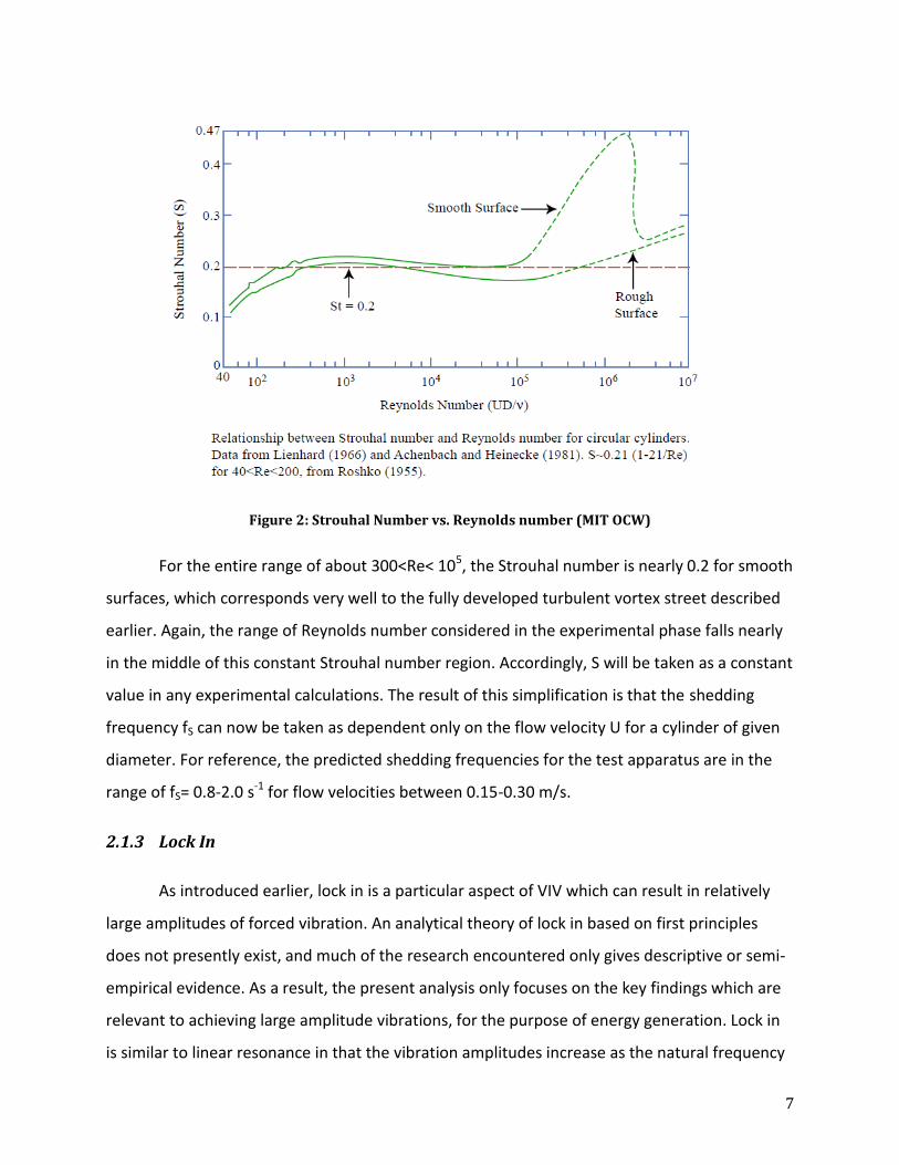
Figure 2: Strouhal Number vs. Reynolds number (MIT OCW)
For the entire range of about 300<Re< 105, the Strouhal number is nearly 0.2 for smooth
surfaces, which corresponds very well to the fully developed turbulent vortex street described
earlier. Again, the range of Reynolds number considered in the experimental phase falls nearly
in the middle of this constant Strouhal number region. Accordingly, S will be taken as a constant
value in any experimental calculations. The result of this simplification is that the shedding
frequency fS can now be taken as dependent only on the flow velocity U for a cylinder of given
diameter. For reference, the predicted shedding frequencies for the test apparatus are in the
range of fS= 0.8-2.0 s-1 for flow velocities between 0.15-0.30 m/s.
2.1.3 Lock In
As introduced earlier, lock in is a particular aspect of VIV which can result in relatively
large amplitudes of forced vibration. An analytical theory of lock in based on first principles
does not presently exist, and much of the research encountered only gives descriptive or semi-
empirical evidence. As a result, the present analysis only focuses on the key findings which are
relevant to achieving large amplitude vibrations, for the purpose of energy generation. Lock in
is similar to linear resonance in that the vibration amplitudes increase as the natural frequency
8
of the cylinder is approached by the vortex shedding frequency. However, the analogy stops
here, as lock in is a highly non-linear phenomenon, affected by feedback loops referred to as
fluid structure interaction. Additionally, lock in does not result in the classic large amplitude
spike at exactly the natural frequency, as in linear resonance. Instead, lock in has been
described as both a self-limiting and self-governing occurrence, as the cylinder vibrations
themselves effect the vortex shedding process, and vice versa. It is self-limiting in the sense that
as the cylinder displacement increases, the vortex shedding is weakened, and hence tends to
reduce further motion. Detailed experimental studies have shown that at large amplitude
vibration, the vortex shedding pattern can be changed from the typical two vortices per cycle to
three, as well as other unsteady combinations (Blevins).
The most important result from lock in studies has been that the phenomenon can
occur over very wide ranges of shedding frequencies. This means that even at shedding
frequencies significantly different than the bodies’ natural frequency, the cylinder-vortex street
interaction may still cause the shedding frequency to suddenly shift, matching the natural
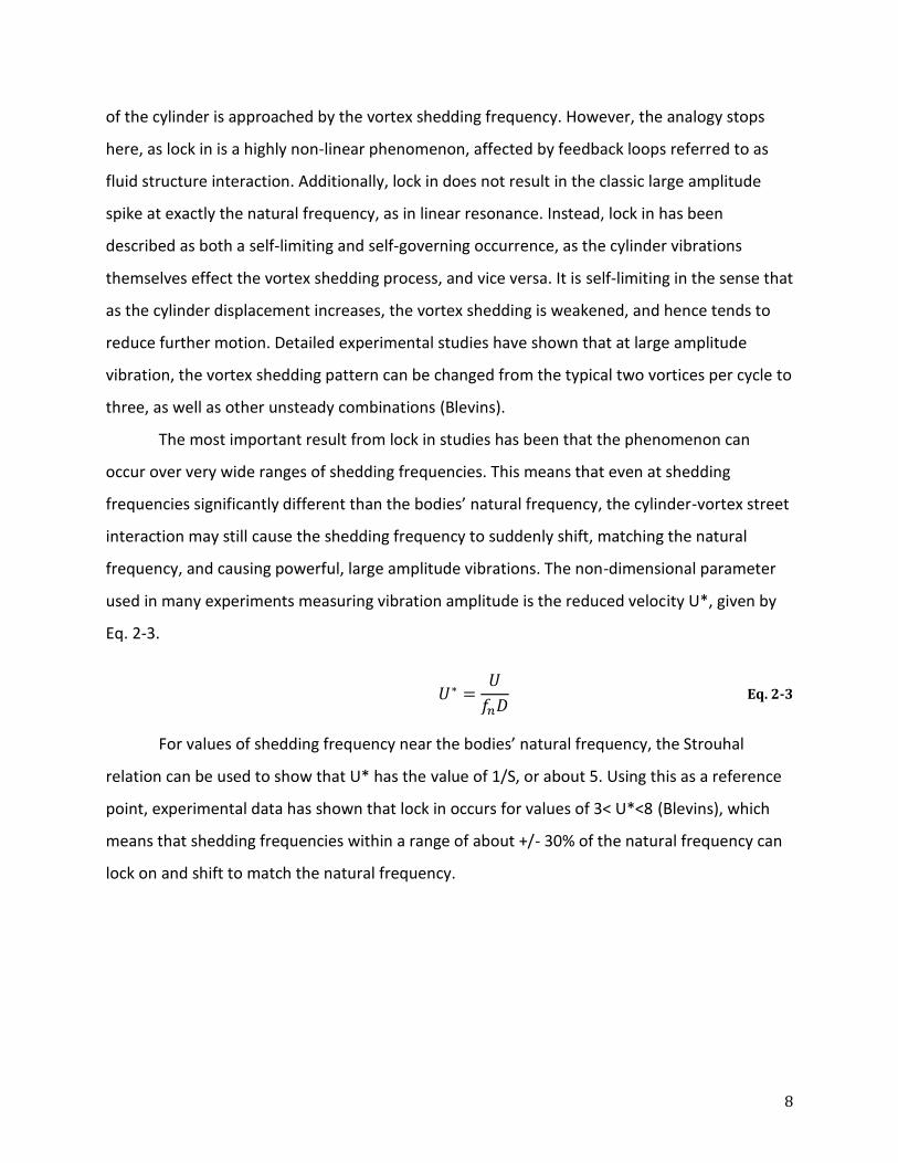
frequency, and causing powerful, large amplitude vibrations. The non-dimensional parameter
used in many experiments measuring vibration amplitude is the reduced velocity U*, given by
Eq. 2-3.
Eq. 2-3
For values of shedding frequency near the bodies’ natural frequency, the Strouhal
relation can be used to show that U* has the value of 1/S, or about 5. Using this as a reference
point, experimental data has shown that lock in occurs for values of 3< U*<8 (Blevins), which
means that shedding frequencies within a range of about +/- 30% of the natural frequency can
lock on and shift to match the natural frequency.

9
Figure 3: Reduced Velocity vs. Mass Ratio (Williamson and Govardhan)
To further complicate things, studies reviewed by (Govardhan, 2004) have shown that
the range over which lock in occurs has a strong dependence on another non-dimensional
parameter, the mass ratio m*, defined as ⁄ , where md is the displaced fluid mass, or
simply the cylinder volume multiplied by the fluid density. For large values of m*, the lock in
range does not vary significantly as the oscillating mass is changed. However, as seen in Figure
3, as the value of m* approaches 2, the upper limit of the lock in range begins to grow
exponentially.
By extrapolating the data outward, it was found that at a mass ratio of 0.54, the lock in
region extended to infinity on the upper side, suggesting that this value was a type of “critical
mass” for VIV (Govardhan, 2004). This phenomenon has also been taken into consideration for
the test apparatus, as the mass ratio m* for the considered 1.25” PVC cylinder has been
calculated as ~0.46. However, it is unknown if this will have the desired effect of expanding the
lock in region, as it is additionally noted that this phenomenon is only applicable to systems of
low reduced mass-damping product, given by the criteria (m* + 1)ζ <0.05. The damping
10
considered for the test apparatus may meet this criterion; however, much greater damping will
need to be added for the implementation of a power take off system, and will definitely be well
above ζ=0.03, which is the limit for satisfying the criterion.
2.1.4 Boundary Gap
Another modeling constraint affecting the oscillation of the cylinder is the boundary gap
ratio. The gap ratio is equal to the minimum distance between the cylinder and lower flow
surface boundary divided by the diameter of the cylinder. (Raghavan, Bernitsas, & Maroulis,
2009) demonstrated that the coefficient of viscous drag and lift coefficient were directly related
to the gap ratio. As the gap ratio increases, viscous drag decreases and lift increases. This is due
to the effect of the gap ratio on vortex shedding. When the cylinder is in close proximity to the
flow surface boundary, flow over the cylinder is uneven. Normal vortex shedding patterns are
weakened or disrupted completely. It was found that, for a boundary gap value of about 3.0 or
greater, the effect of the boundary gap on vortex shedding was negligible. To calculate an
appropriate gap distance for a 1.25” diameter cylinder, as will be used in the test apparatus,
multiply the cylinder diameter by three: 3*1.25” = 3.75”. This yields a gap ratio of 3, rendering
the effects of the boundary on vortex shedding negligible.
11
2.2 VIVACE
The Vortex Induced Vibration Aquatic Clean Energy converter design was patented in
2008 by Professor Michael Bernitsas of the University of Michigan. The converter harnesses
energy from water flow using vortex induced vibrations.
The VIVACE system is composed of a cylinder secured horizontally in a stationary frame
and allowed to oscillate transverse to the direction of water flow. The cylinder is connected to
the frame at the ends of the cylinder, where magnetic sliders move up and down over a rail
containing a coil. The motion of the magnet over the coil creates a DC current, which can be
stored or converted to AC to be sent into the grid.
This technology is superior to dam technology in several ways. It is capable of producing
energy from fluid flow without altering the local environment, posing any danger to nearby
residents, changing the landscape in any visible way, or interfering with water traffic in any slow
moving waterway (0.5-5 knots). Energy generation from VIV has significant potential for coastal
areas as well. Fifty percent of the U.S. population lives within 50 miles of the coast, whereas
this coastal land accounts for only 11 percent of U.S. territory. Energy demand in coastal
regions is much larger than demand inland.
Scalability and versatility are two of the greatest strengths of this technology. Modules
can range in size from single-cylinder arrays to thousand-cylinder, mega-watt producing power
plants. In their initial report, Bernitsas et al. outline array specifications for 1kW to 1000MW
cylinder arrays. Areas of potential power production include ocean water bodies and rivers.
Flow in the prime production speeds required for this technology is significantly lower than for
other turbine based hydrokinetic technologies.
According to Bernitsas, VIVACE has superior energy density compared with other non-
turbine ocean energy technologies. As of August 2010, Bernitsas’ start-up company, Vortex
Hydro Energy, has begun open water tests in the St. Clair River in Port Huron, MI.

12
3 Modeling
In order to establish estimates of the potential dynamic performance of a VIV based
energy harnessing device, a relatively simple mathematical model was constructed to describe
the fluid-oscillator interaction. This section seeks to explain this process and also demonstrate
the results for one particular cylinder size. Since a basic concept of how the testing would later
be carried out had already been established, many physical parameters of the setup were
known or at least bounded within a specific range. The initial model calculations were based on
the use of a 1.25 in nominal diameter PVC pipe section, and the geometrical and fluid
properties show in Table 1.
Property Variable Value
Cylinder diameter D 0.042 m
Cylinder length L 0.22 m
Linear cylinder density ρcyl 0.64 kg/m
Water density ρfluid 998 kg/m3
Water kinematic viscosity ν 1.31E-6 m2/s
Maximum flow speed U 0.35 m/s
Table 1: Cylinder and Flow Parameters
All fluid properties were taken at 20°C, sine the experiments were carried out at room
temperature. Although the flow velocity was one of the main variables under control during the
experimental phase, the maximum value achieved was used here to establish upper limits on
performance. Eq. 3-1 below shows the value of the Reynolds number based on initial
parameters.
Eq. 3-1
For 300<Re< 3x10⁵, the vortex street behind the cylinder is known to be fully turbulent,
and strong, periodic shedding results. Accordingly, for a fixed pipe size, a wide range of flow
velocities are possible while still resulting in a suitable value of Reynolds number for vortex
shedding to occur.

13
The Strouhal number determines the vortex shedding frequency as an empirical
function of Re over a wide range of flow speeds (Eq. 3-2).
(
) Eq. 3-2
The Strouhal number is insensitive to Reynolds number and thus flow speed, as S remains
nearly constant for 103<Re<105. For this reason, the S will be treated as a constant throughout
the experiment. The vortex shedding frequency fS is then calculated from Eq. 3-3.
Eq. 3-3
This will be the main variable of interest for achieving large amplitude vibrations, since it must
be matched to the natural vibration frequency of the cylinder in order to achieve large
amplitude vibrations.
In the experiments, the vortex shedding frequency will be determined by the flow
conditions and cylinder size. To match the cylinder’s natural frequency to the vortex shedding
frequency, the following cylinder properties were determined.
Eq. 3-4
Eq. 3-5
Eq. 3-6
Eq. 3-7
Eq. 3-8
Mass madd (Eq. 3-6) represents additional mass added to the pipe, which will initially be
set as 0. The pipe mass mpipe (Eq. 3-7) was determined based on unit length density of
0.64kg/m. The term mdis (Eq. 3-5) represents the mass of fluid displaced by the cylinder, and
must be added to take into account the force which must be exerted as the cylinder pushes the
fluid out of its path. The apparent mass of the pipe in the fluid is then given by Eq. 3-8 as the
sum of the pipe mass and displaced fluid mass. It is this value of apparent mass which should

14
then be used to determine the natural frequency of the cylinder in water. The natural
frequency of vibration is determined in Eq. 3-9.
√
Eq. 3-9
For this particular system, k represents the stiffness of the springs used to suspend the
pipe, which will be controlled approximately to 0.2 lbf/in. This value of k was chosen to match
the natural frequency to the shedding frequency. For these chosen values, the frequency ratio
f* is equal to 1.041, which is well within the ± 30% lock-in range.
The motion of the cylinder was modeled by a general equation of motion for linear
vibration (Eq. 3-10).
Eq. 3-10
This model is only an approximation due to the non-linear nature of vortex shedding;
however, experimental studies have shown that this approximation is accurate. This equation
includes the term m*y’’ representing the inertia of the cylinder, 2mζ ny’ representing the
viscous drag force (damping), and the restoring force k*y. A value of 0.06 is assumed for ζ based
on experimental findings of similar vortex induced vibration studies. F(t) represents the periodic
force exerted on the cylinder by the vortices. In this model, F(t) is assumed to be a sinusoidal
function with frequency equivalent to natural frequency of the cylinder, representing the
condition of lock-in. The equation for FL (Eq. 3-11) comes from the definition of lift force and
gives the amplitude of F(t).
Eq. 3-11
Coefficient of lift CL is assumed to be 0.6 as a conservative estimate based on
background research. Realistically, CL varies with displacement of the cylinder, so this value is
an average. The solution for the amplitude of the cylinder vs. time is given by Eq. 3-12. Figure 4
shows cylinder amplitude in terms of cylinder diameter as a function of time.

15
( )
√( (
)
)
(
)
Eq. 3-12
Figure 4: Cylinder Amplitude over Diameter as a Function of Time
Velocity of the cylinder is found by differentiating the equation for displacement with
respect to time (Eq. 3-13), and is shown in Figure 5.
Eq. 3-13
0 0.2 0.4 0.62
1
0
1
2
yres t( )
Dpipe
t

16
Figure 5: Derived Cylinder Velocity
Maximum velocity of the cylinder is about 0.5 m/s at the point where cylinder
displacement is zero.
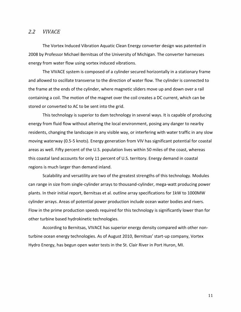
Power is determined by the product of the velocity and force of lift exerted on the
cylinder by vortex shedding (Eq. 3-14). As seen in Figure 6, the frequency of P(t) is twice the
frequency of either v(t) or FL since it contains the product of sine and cosine.
Eq. 3-14
0 0.2 0.4 0.61
0.5
0
0.5
1
v t( )
t
17
Figure 6: Cylinder Power with Defining Parameters
Maximum power amplitude is calculated to be 0.063W. Average power for the cylinder
is determined in Eq. 3-15. The theoretical upper limit of power in the fluid is represented by Eq.
3-16.
√ Eq. 3-15
=0.18W Eq. 3-16
Eq. 3-16 is derived from the product of force exerted on the cylinder by fluid flow and
flow velocity. Efficiency η is calculated to be:
Eq. 3-17
This efficiency falls within the range shown in VIVACE studies, although VIVACE power output
was much larger.
0 0.2 0.4 0.61
0.5
0
0.5
1
P t( )
FL sin n t
v t( )
t
18
4 Methodology
This section discusses the physical set up of the flow tank and all components. A design
process is discussed, including the reasoning behind selection of the tank design and sensor
type. The experimental progression followed throughout this project is outlined.
4.1 Experimental Setup
In order to test the VIV phenomenon, an open channel flow tank was needed. Sump
pumps were researched based on pumping capacity and price. From our initial calculations, a
flow speed of 0.35 m/s through the channel area matched the Reynolds number range we
wanted (Re = 300 to 3*105), and was calculated to require a volumetric flow rate of 30,920
gallons per hour (GPH). It was later found using a flow rate sensor that the recirculating nature
of the tank allowed channel flow speeds of up to 0.32 m/s with a total of only 9,130 GPH total
pump capacity.
The objective of the tank design was to provide a uniform and steady flow speed within
a data collection area. The initial tank design was for a circular flow tank of 4' diameter, but at
the expected flow speeds it was anticipated that uneven flow velocity across a channel cross
section due to the curve of the tank would be problematic. The final recirculating tank design
was reached, which eliminated these problems, and provided a consistent flow through the test
area.
To measure the energy flow rate of the cylinder during vibration, it was necessary to
measure the acceleration and displacement of the cylinder in the water, as well as flow
velocity. Measurement systems that would work under water were initially considered. A linear
slider pushed by the cylinder to the distance of its maximum amplitude was initially considered;
that method recorded only maximum amplitude, not amplitude over time. Laser Doppler
velocimetry was researched for the purpose of measuring flow velocity and flow patterns, but
required the use of a dye in the water to make readings. It was found through testing that dye
in the moving water dispersed within a matter of a few seconds and the water color quickly
became uniform. The technology was also found to be too expensive. The final set up involved

19
the measurement of movement of an out of water platform supported over the cylinder using a
sonic motion sensor, and use of propeller type flow sensor placed in the central channel.
4.1.1 Materials
The following materials and equipment were used in the set up.
1. 6’x2’x2’ water tank
2. 5 gallon bucket
3. Schedule 40 PVC pipe, 0.75”-2.0” diameter
4. 3125 GPH sump pump (2)
5. 2880 GPH sump pump
6. 0.75”x16”x48” boards (3)
7. Aluminum stock
8. Extension spring (4)
9. Vernier Flow Rate Sensor
10. Vernier MD BTD (Displacement Sensor)
11. Vernier LabPro
12. Logger Pro Computer Software
4.1.2 Description
The experimental set-up was assembled within a 6’x2’x2’ water tank using. Data was
collected within a central channel 4’ long by 11¾” wide placed in the center of the tank. Figure
7 and Figure 8 show the channel within the tank.

20
Figure 7: Tank and Channel Top View
Figure 8: Tank and Channel Isometric View
On one end of the tank, sump pumps drew in water and pumped it towards the other end via
the two thin channels created between the walls of the central channel and the walls of the
tank. The two side pumps were rated at 3125 GPH each and the central pump was rated at
2880 GPH. The piping used for the pumps was 1.25” diameter schedule 40 PVC pipe and pipe
components. For each of the two side pumps, a threaded connector, an elbow, and a 16”
length of straight pipe were used. For the central pump, a threaded connector, a ball valve, a T
split, two 7” lengths, two elbows, and two 16” lengths were used. The valve allowed
adjustment of the flow velocity during testing.
21
On the other end of the tank, two flow guides served to merge flow from the side
channels and direct it through the central channel. The purpose of the flow guides was to
redirect flow in the smoothest manner possible. Since the test channel was short, it was
important to smooth the flow as much as possible before it reached the cylinder testing area.
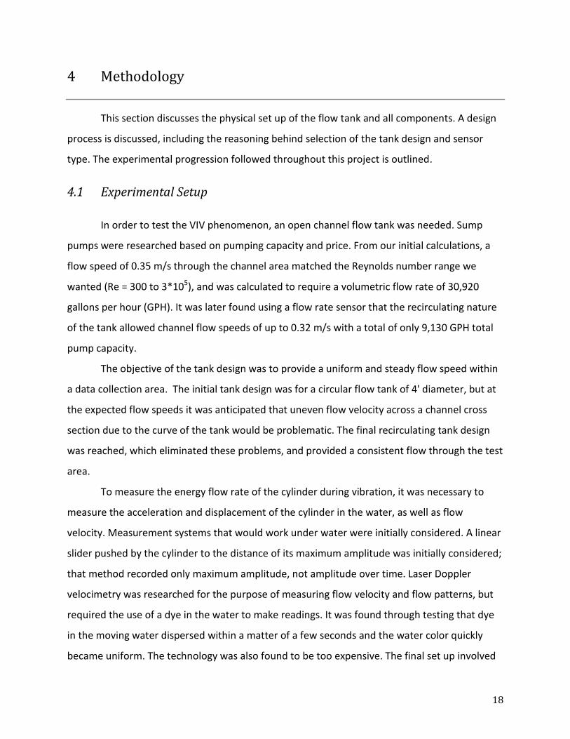
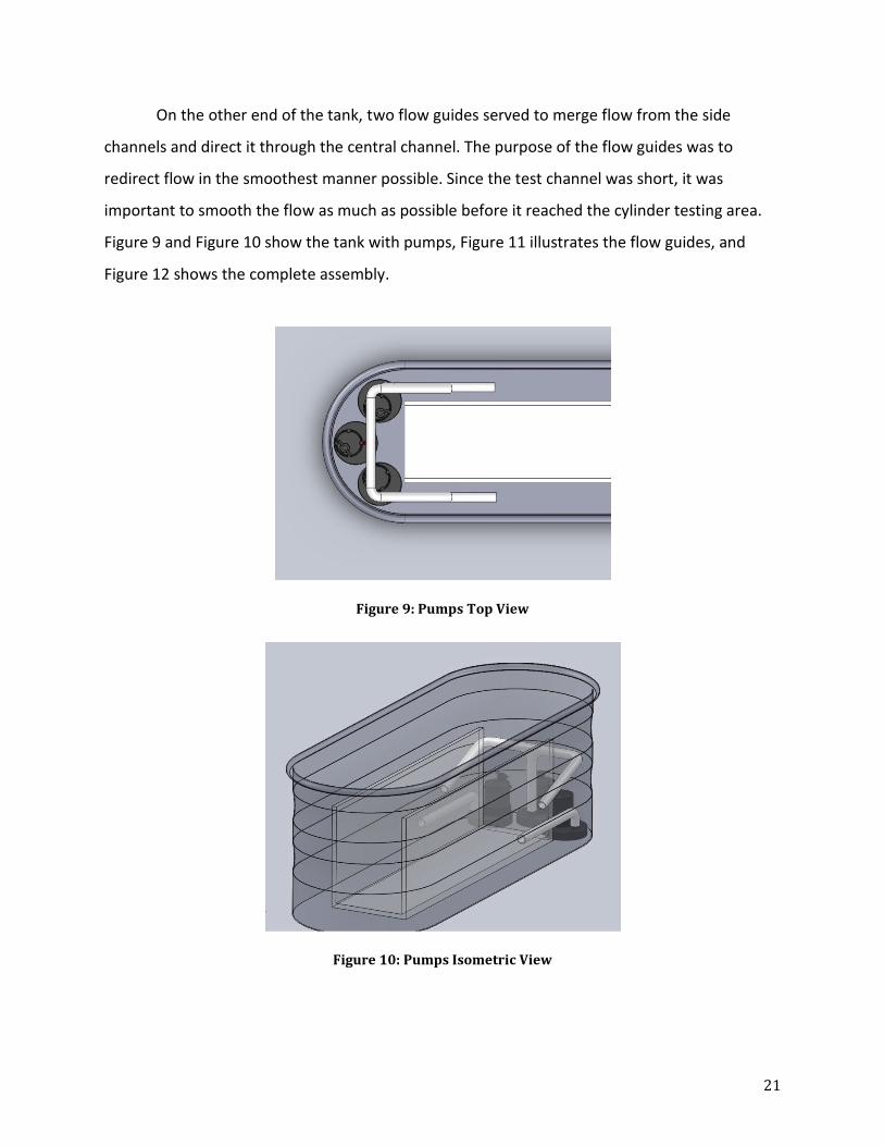
Figure 9 and Figure 10 show the tank with pumps, Figure 11 illustrates the flow guides, and
Figure 12 shows the complete assembly.
Figure 9: Pumps Top View
Figure 10: Pumps Isometric View

22
Figure 11: Flow Guides Top View
Figure 12: Tank with Pumps and Flow Guides
Initially, walls were placed in the side channels with holes fit to and secured around the
sump pump pipes in order to block any flow unless pumped through the pipes. These were
intended to prevent flow from pumps returning directly back to the pump inlet without first
circulating through the center channel, but they were found to restrict tank flow and decrease
overall flow speed.
Five cylinders of varying diameter were constructed from PVC schedule 40 piping. All
cylinders were approximately nine inches in total length, with ¾”, 1”, 1 ¼”, 1 ½”, and 2” nominal
diameters. The true outer diameters of these cylinders were 1.050”, 1.315”, 1.660”, 1.900”, and
2.375” respectively. Stock PVC end caps were pressed onto the ends of the cylinders to seal
23
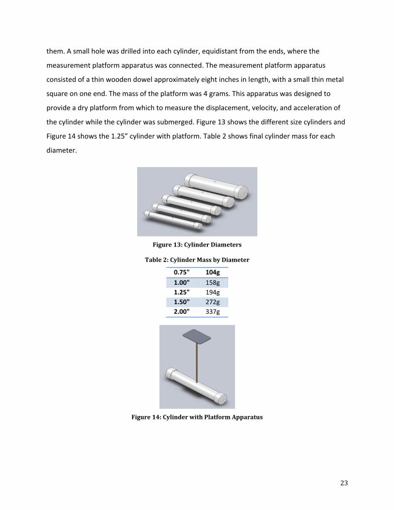
them. A small hole was drilled into each cylinder, equidistant from the ends, where the
measurement platform apparatus was connected. The measurement platform apparatus
consisted of a thin wooden dowel approximately eight inches in length, with a small thin metal
square on one end. The mass of the platform was 4 grams. This apparatus was designed to
provide a dry platform from which to measure the displacement, velocity, and acceleration of
the cylinder while the cylinder was submerged. Figure 13 shows the different size cylinders and
Figure 14 shows the 1.25” cylinder with platform. Table 2 shows final cylinder mass for each
diameter.
Figure 13: Cylinder Diameters
Table 2: Cylinder Mass by Diameter
0.75" 104g
1.00" 158g
1.25" 194g
1.50" 272g
2.00" 337g
Figure 14: Cylinder with Platform Apparatus
24
Holes were drilled into the end caps oriented concentric to the cylinder pipe. Pre-cut
wooden dowels were inserted into the end cap holes to provide a location about which to wrap
the ends of the springs. Two or four springs were used, with one or two on each side in parallel
to each other. These springs were attached at the other ends to the cylinder housing. Springs
were selected based on calculations from the mathematical model. In order to achieve lock-in
range, for cylinders of the given mass and given flow speed, total spring stiffness needed to be
close to 46N. Springs used in the final set up had a stiffness of 12N each, for a total stiffness of
48N.
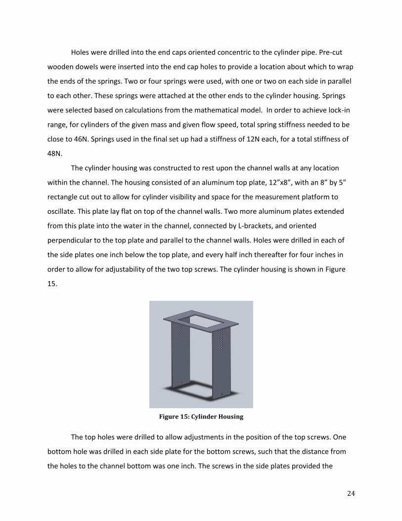
The cylinder housing was constructed to rest upon the channel walls at any location
within the channel. The housing consisted of an aluminum top plate, 12”x8”, with an 8” by 5”
rectangle cut out to allow for cylinder visibility and space for the measurement platform to
oscillate. This plate lay flat on top of the channel walls. Two more aluminum plates extended
from this plate into the water in the channel, connected by L-brackets, and oriented
perpendicular to the top plate and parallel to the channel walls. Holes were drilled in each of
the side plates one inch below the top plate, and every half inch thereafter for four inches in
order to allow for adjustability of the two top screws. The cylinder housing is shown in Figure
15.
Figure 15: Cylinder Housing
The top holes were drilled to allow adjustments in the position of the top screws. One
bottom hole was drilled in each side plate for the bottom screws, such that the distance from
the holes to the channel bottom was one inch. The screws in the side plates provided the
25
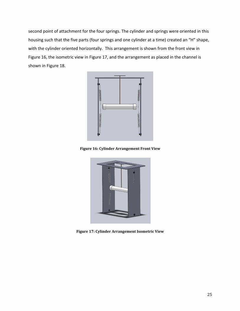
second point of attachment for the four springs. The cylinder and springs were oriented in this
housing such that the five parts (four springs and one cylinder at a time) created an “H” shape,
with the cylinder oriented horizontally. This arrangement is shown from the front view in
Figure 16, the isometric view in Figure 17, and the arrangement as placed in the channel is
shown in Figure 18.
Figure 16: Cylinder Arrangement Front View
Figure 17: Cylinder Arrangement Isometric View

26
Figure 18: Cylinder Arrangement in Channel
Two nails were inserted into the inner channel walls near the inlet, one on each side. A
three foot length of thin metal wire was tied to each nail. The wires ran along the channel walls
and attached at the other end to the wooden dowels protruding from the cylinder end caps.
These wires restricted the cylinder from moving downstream within the channel, and limited its
motion to a nearly vertical direction. The proper placement of the cylinder housing in the
channel was determined from the wire connection by noting the point at which the springs
appeared to be closest to vertical when the water was flowing. The full tank set up is shown in
Figure 19.

27
Figure 19: Test Set Up
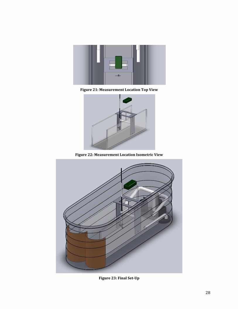
Data was taken with two Vernier instruments, the Vernier Flow Rate Sensor and the
Vernier MD BTD (Displacement Sensor). The MD BTD recorded displacement data from the dry
oscillating platform supported over the cylinder, from which the computer software (Logger Pro
3) extrapolated velocity and acceleration data. The propeller type Flow Rate Sensor had a three
inch diameter rotor and allowed us to measure flow in any small section of the tank. To create a
flow velocity profile of the channel, flow rate was measured at three channel heights at five
locations in the channel moving from right to left. The MD BTD is shown in Figure 20 (left) along
with the Flow Rate Sensor (right), and the two devices are shown in approximate measurement
positions within the tank in top view (Figure 21) and isometric view (Figure 22 and Figure 23).
Figure 20: Vernier MD BTD Sensor and Flow Rate Sensor
28
Figure 21: Measurement Location Top View
Figure 22: Measurement Location Isometric View
Figure 23: Final Set-Up
29
4.2 Experimental Procedure
To compare the response of the physical system to that of the mathematical model, a
number of parameters needed to be determined experimentally. Displacement, velocity, and
acceleration were measured directly using the motion sensor. Flow velocity was measured
using the impeller flow sensor. Mass was measured using an electronic scale, and diameter of
the cylinders was measured with calipers. All other data from experiments was derived directly
or indirectly from these measured values. The relationships between the measured and derived
variables are discussed with more depth in the Analysis chapter of this report.
The mathematical model assumed a steady flow profile across the entire length of the
cylinder. Once the flow tank had been constructed, the validity of this assumption was tested
experimentally. The differential equation for the response of the system includes variables of
spring stiffness, damped natural frequency, and the damping ratio. These values were
determined experimentally as explained below. The displacement, velocity, and acceleration of
cylinders subjected to fluid flow were measured using the motion sensor.
4.2.1 Data Collection
The Vernier MD-BTD Motion Detector 2 measures the position of objects with the use of
ultrasound waves. The detector has a range of 0.15m to 6m and a resolution of 1mm. The
detector can be zeroed based on the neutral position of a stationary object. The maximum
sampling rate is 50Hz.
The Vernier FLO-BTA Flow Rate Sensor measures the velocity of flowing water. The
sensor consists of an impeller. The rotational speed of the impeller is proportional to the speed
of the flowing water. A magnet in the impeller triggers a switch with each half rotation. The
switch creates a pulse that the signal conditioner then converts to a voltage that is proportional
to the flow velocity. This device is pre-calibrated by the manufacturer. The sensor has a range
of 0 to 5 m/s, a resolution of 0.0012m/s, and a response time of 98% of full scale reading in 5s.
The Vernier LabPro is a data collection interface that is compatible with both the motion
detector and the flow rate sensor. The Motion Detector connects to a digital input of the
LabPro device. The Flow Rate Sensor connects to an analog input of the LabPro device. When

30
LabPro is connected to a computer through a USB cable, it works in conjunction with the
LoggerPro computer software. The device automatically detects the sensors currently
connected and creates the appropriate interface with the software. This allowed data for both
flow velocity and cylinder displacement to be measured and displayed simultaneously.
Recording of data begins and ends by pressing collect. A sampling rate and sampling time can
be defined by the user. The raw data from the experiment can be imported to an excel
spreadsheet with the appropriate headers for each data type intact. The LoggerPro interface
used for the experiment is shown in Figure 24.
Figure 24: The LoggerPro Interface
31
4.2.2 Flow Profile Measurements
1. Use a test tube clamp to hold the flow meter
2. Insert the flow meter into the top corner of the central channel, facing the flow and
approximately 1 meter away from the entrance of flow into the channel
3. Record the flow for 30 seconds at a sampling rate of 4 samples per second
4. Repeat steps 1-3 at all locations of the flow profile defined in Table 3, with and without
the diffuser
Table 3: Flow Profile Locations
Top 1 Top 2 Top 3 Top 4 Top 5 Middle 1 Middle 2 Middle 3 Middle 4 Middle 5 Bottom 1 Bottom 2 Bottom 3 Bottom 4 Bottom 5
4.2.3 Spring Stiffness
1. Hang spring from ring stand; Place the motion sensor below the spring
2. Attach known mass to the free end of the spring
3. Zero the motion sensor at the neutral position for the spring-mass system using
LoggerPro
4. Extend the spring approximately 1” and release so that the system begins to oscillate
5. Begin recording with the motion sensor; record for 20 seconds with a sampling rate of
30 samples per second
6. Find the natural frequency based on the recorded displacement data: ω=n/t; where ω is
the natural frequency, n is the number of oscillations, and t is the time
7. Calculate stiffness with the following formula: k=ω2*m; where k is stiffness and m is
mass
8. Repeat steps 1-7 for all springs to be used in the experiments
9. Sum the stiffness of each spring used in a setup to determine the equivalent stiffness of
the parallel springs
4.2.4 Cylinder Dimensions
1. Use electronic scale to measure mass of the cylinder; include end caps, and dowel pins
2. Measure the length of cylinder using a ruler
3. Measure the diameter of the cylinder using calipers
4. Repeat steps 1-3 for all cylinders to be used in the experiments

32
4.2.5 Natural Frequency and Damping
1. Set up the spring-cylinder system as described earlier
2. Place the system in water so that the cylinder is completely submerged
3. Use a ring stand to hold the motion sensor 0.15-0.5m above the cylinder
4. Push down on the cylinder and release so that the system begins to oscillate
5. Begin recording with the motion sensor; record for 20 seconds with a sampling rate of
30 samples per second
6. Find the damped natural frequency based on the recorded displacement data
7. Find the damping ratio based on the recorded displacement data: This derivation is
discussed in the Analysis chapter
8. Repeat steps for different cylinder diameter-mass combinations; these are summarized
in Table 4
Table 4: Damping Test Configurations
pvc Diameter (m) configuration Mass (g)
.75" 0.0267 4 springs 135
.75" 0.0267 4 springs 152
1" 0.0334 4 springs 155
1" 0.0334 4 springs 172
1.25" 0.0422 4 springs 195
1.25" 0.0422 4 springs 212
1.5" 0.0483 4 springs 272
1.5" 0.0483 4 springs 289
2" 0.0603 2 springs 343
2" 0.0603 2 springs 377
33
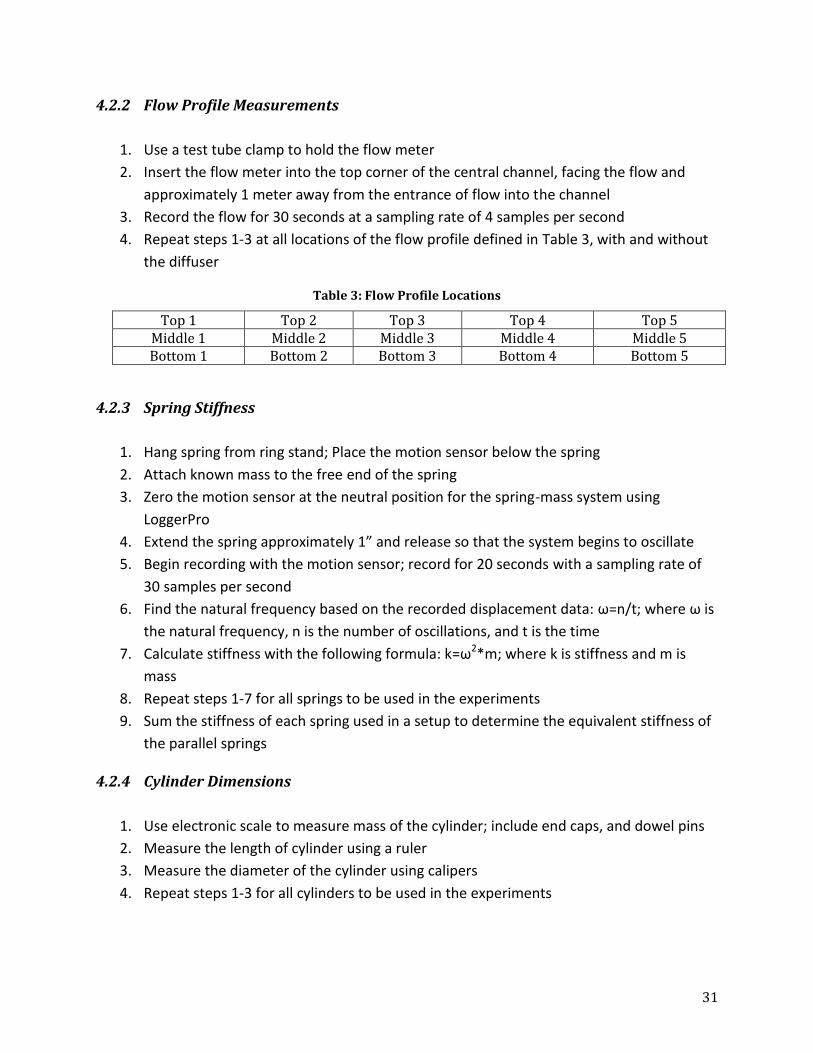
4.2.6 Cylinder Displacement
1. Set up the spring-cylinder system as described earlier
2. Begin flow in the tank at a low speed
3. Once the cylinder begins to oscillate, record displacement and flow speed for 60
seconds with a sampling frequency of 20 samples per second
4. Increase the flow speed and repeat; flow speed was increased 5 times for each cylinder-
mass configuration
5. Repeat steps 1-4 with different cylinder diameter and mass configurations; the
configurations used are summarized in Table 5
Table 5: Cylinder Diameter-Mass Configurations Used in Experiments
PVC Size Mass # of Springs
0.75" 104g 4
0.75" 121g 4
0.75" 138g 4
0.75" 155g 4
1" 158g 4
1" 175g 4
1" 192g 4
1" 209g 4
1.25" 195g 2
1.25" 212g 2
1.25" 229g 2
1.5" 272g 4
1.5" 306g 4
1.5" 340g 4
2" 337g 2
2" 405g 2

34
5 Analysis and Results
This chapter presents the details of the data handling processes used in the project, as
well as the final results that were produced from the collected data. Section 1 focuses on the
data analysis methods used, and overviews the flow and reduction of data throughout the
project. Section 2 presents a summary of the significant findings that were produced from the
analysis, as well as references to the final data presented in tabular form in the appendices.
5.1 Data Analysis and Reduction Process
Throughout the experimental phase of the project, a large number of parameters were
calculated based on data, theory, and a combination of both. This entire process is best
summarized by Figure 25.
Figure 25: Experimental Data Flowchart
Measurements
· Cylinder displacement vs time
Still water decay tests
Measurements
· Cylinder displacement, velocity, & acceleration vs time
· Flow velocity vs time
Flowing water tests
· Calculate peak oscillation frequency using FFT
· Calculate mean flow speed and mean deviation
· Plot V vs X (phase portrait) to evaluate oscillation quality
· Calculate mean amplitude
· Determine fluid force F(t) using inertial, damping, and elastic terms
· Calculate RMS mechanical power using F(t) and V(t)
Analysis
DiameterMass
Stiffness
Cylinder variables
Shedding frequency fshd
Total fluid power
Theory
Oscillation frequency fosc
Mean flow speed and deviationfosc/fn f*
Mean amplitude Xmean
RMS power PRMS
Non dimensional velocity U*Efficiency η
Power coefficient Cp
Reynolds number Re
Final metrics
Natural frequency fn
Damping ratio ζHydrodynamic mass
Derived properties
· Calculate mean natural frequency over three cycles
· Solve for total mass
· Calculate damping using logarithmic decrement over first two cycles
Analysis

35
Here, the process is broken down into the major steps represented by each box. By viewing left
to right, the process starts with the two main sets of measurements, the controlled cylinder
variables, and values calculated from basic VIV and fluid theory. From here, the cylinder
variables and still water tests are combined and passed through an analysis to produce the
derived cylinder properties. The cylinder variables, flowing water tests, and derived properties
are then passed through a second analysis, which is then combined with theory and the derived
properties to produce the final metrics. The details of each of these sub-processes are
described in the sections that follow.
5.1.1 Still Water Decay Tests
As introduced in the methodology, the still water decay tests consisted of measuring
cylinder displacement vs. time, at 20 samples/s, after applying an initial disturbance to the
cylinders in water. The data produced from these tests consisted of 5 second time series for
each trial. Overall, 5 trials were performed for each cylinder configuration, which consisted of
two different masses for each of the five cylinder diameters, giving a total of 50 data sets. From
these data, the known cylinder diameters, masses and spring stiffness were used to determine
the natural frequency (in water), damping ratio, and hydrodynamic mass of each of the five
cylinders at two different values of cylinder mass. The details of these calculations are
presented in the sub sections that follow. For the final summarized resultant data, see Table 6.
Table 6: Free Decay Test Summary Data
PVC Diameter
(m) configuration
Length (m)
Mass (g)
k (N/m)
Frequency (hz)
Zeta 1 actual added
mass (g) predicted added
mass (g) ratio
(actual/predicted)
.75" 0.0267 4 springs 0.22 135 47.6 1.860 0.107 214 123 1.74
.75" 0.0267 4 springs 0.22 152 47.6 1.802 0.067 219 123 1.78
1" 0.0334 4 springs 0.22 155 47.6 1.598 0.067 317 192 1.65
1" 0.0334 4 springs 0.22 172 47.6 1.587 0.067 307 192 1.59
1.25" 0.0422 2 springs 0.22 195 23.8 1.333 0.075 144 307 0.47
1.25" 0.0422 2 springs 0.22 212 23.8 1.324 0.074 132 307 0.43
1.5" 0.0483 4 springs 0.22 272 47.6 1.170 0.060 609 402 1.51
1.5" 0.0483 4 springs 0.22 289 47.6 1.138 0.052 642 402 1.60
2" 0.0603 2 springs 0.22 343 23.8 0.688 0.052 931 627 1.48
2" 0.0603 2 springs 0.22 377 23.8 0.683 0.050 916 627 1.46
36
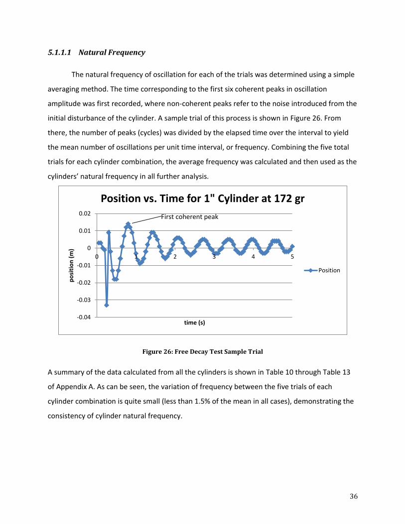
5.1.1.1 Natural Frequency
The natural frequency of oscillation for each of the trials was determined using a simple
averaging method. The time corresponding to the first six coherent peaks in oscillation
amplitude was first recorded, where non-coherent peaks refer to the noise introduced from the
initial disturbance of the cylinder. A sample trial of this process is shown in Figure 26. From
there, the number of peaks (cycles) was divided by the elapsed time over the interval to yield
the mean number of oscillations per unit time interval, or frequency. Combining the five total
trials for each cylinder combination, the average frequency was calculated and then used as the
cylinders’ natural frequency in all further analysis.
Figure 26: Free Decay Test Sample Trial
A summary of the data calculated from all the cylinders is shown in Table 10 through Table 13
of Appendix A. As can be seen, the variation of frequency between the five trials of each
cylinder combination is quite small (less than 1.5% of the mean in all cases), demonstrating the
consistency of cylinder natural frequency.
-0.04
-0.03
-0.02
-0.01
0
0.01
0.02
0 1 2 3 4 5
po
siti
on
(m
)
time (s)
Position vs. Time for 1" Cylinder at 172 gr
Position
First coherent peak

37
5.1.1.2 Damping Ratio
The damping ratio for each cylinder combination was determined using the logarithmic
decrement method. The same combination of data sets as the natural frequency calculations
were used. However, in this case, the amplitudes of the first three coherent peaks were
recorded instead. From Figure 26, it is clear why only the first three oscillation peaks were used.
It appears that after the third peak, oscillation amplitude levels out to a constant value, and
ceases to decay any further during the time interval sampled. From observations made during
the data collection, it is theorized that the wave-like disturbances created by the cylinder while
oscillating were reflected throughout the test tank. Upon returning to the cylinder, these waves
likely sustained the cylinder oscillations when they would normally continue to decay in
amplitude.
The values of the first three oscillation peaks were first used to define a new value δ,
where
, and Ai represents the amplitude of the ith peak. Since three values of Ai
were used, two corresponding δ’s were calculated. From here, the damping ratio ζ was
calculated from Eq. 5-1.
√ Eq. 5-1
This method produced two values of the damping ratio for each trial, as can again be seen for
all cylinders in Appendix A. Unlike the natural frequency data, the values of ζ for each trial
showed significant variation both between one another and between trials. Again, the mean
value of the damping ratio was determined from the five values calculated for each cylinder
combination. In light of the wave-like disturbances mentioned previously, it was decided that
only the first of the two sets of ζ’s from each trial would be used, since they were less likely to
be influenced by the disturbances. In the calculations that followed, it was these mean values of
ζ1 which were used for each cylinder combination.

38
5.1.1.3 Hydrodynamic Mass
As introduced in the modeling chapter, hydrodynamic mass refers to the additional
mass which is effectively added to the cylinder by the fluid it displaces. The theory for
cylindrical bodies states that this mass is equal to the mass of the fluid occupied by a volume
equal to that of the cylinder. To determine this value for the different cylinder combinations,
the previously calculated natural frequencies were used in combination with the known
cylinder masses and spring stiffness.
Basic vibration theory gives the damped natural frequency of a body as Eq. 5-2,
√
√ Eq. 5-2
where k is the total stiffness and m is the total mass. By solving for the total mass and then
subtracting the known cylinder mass, the hydrodynamic added mass was effectively
determined. Since this value was determined using mean natural frequencies, only one value is
calculated for each cylinder-mass combination, and the results are again shown in Table 6. As
can be seen there, there was a significant discrepancy between the hydrodynamic mass
specified by theory, and that calculated experimentally. A possible explanation of this can be
given based on the separation distance of the cylinder from the bottom surface of the channel
during the trials. Since this distance was relatively small, on the order of <5 cylinder diameters,
additional “added inertia” could be imparted to the cylinder since the assumption of infinite
fluid, from which added mass theory is based, is not valid. Despite these findings, the flowing
water tests which were to be later conducted would have the same physical setup, so use of
the experimentally determined hydrodynamic masses was an appropriate choice.

39
5.1.2 Flowing Water Tests
As introduced in the methodology, the flowing water tests consisted of 85 total cylinder
trials. For each of the five cylinder diameters, two to four different cylinder masses were used,
and each of those combinations was subjected to four to five unique flow speeds. The specific
testing combinations used were previously listed in the methodology. The data set produced
from each individual trial consisted of a one minute time series of cylinder displacement and
flow velocity. The data logging software also numerically differentiated the displacement data
and included cylinder velocity and acceleration in the data set as well. These data were then
analyzed in combination with the controlled cylinder variables and derived properties found in
section 5.1.1 in order to determine mean flow speed, oscillation frequency, f*, mean oscillation
amplitude, RMS mechanical power, U*, efficiency, power coefficient, and Re for each cylinder
test trial. The details of these calculations are presented in the sub sections that follow. For
reference, a sample of this final data is presented in Table 7 below. The complete results for all
valid tests are then shown in Appendix B.
mean flow (m/s) SD % Fshd (hz) Fosc (hz) osc/shd f* X mean (m) Prms (W) U* η Cp Re A/D
0.250 7.0 1.85 1.92 1.04 0.98 0.013 0.0169 4.79 0.37 0.37 5.09E+03 0.49
0.246 6.8 1.82 1.98 1.09 1.01 0.016 0.0213 4.72 0.49 0.49 5.01E+03 0.60
0.251 6.6 1.86 1.96 1.05 1.01 0.016 0.0213 4.82 0.46 0.46 5.12E+03 0.60
0.273 9.7 2.02 2.10 1.04 1.07 0.018 0.0272 5.24 0.46 0.46 5.56E+03 0.67
0.301 5.8 2.23 2.12 0.95 1.09 0.018 0.0302 5.78 0.38 0.38 6.14E+03 0.67
mean 7.2
0.43 0.43
0.61
Table 7: 0.75" Cylinder Trial 1Final Results
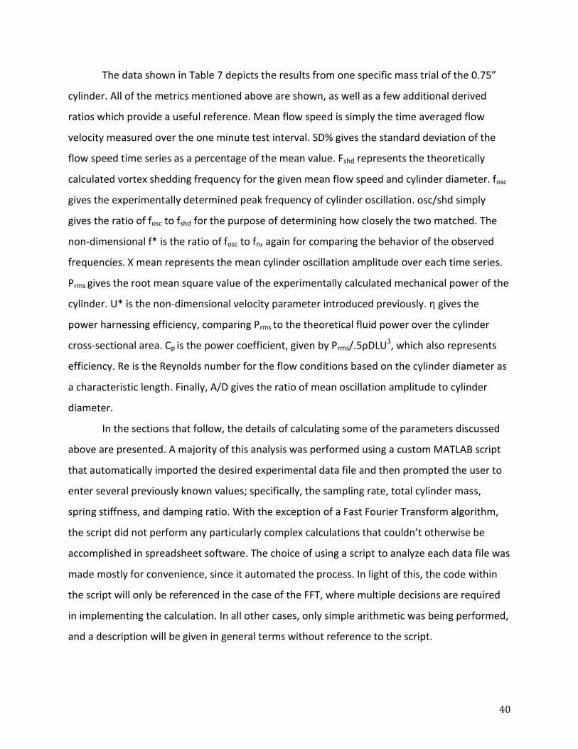
40
The data shown in Table 7 depicts the results from one specific mass trial of the 0.75”
cylinder. All of the metrics mentioned above are shown, as well as a few additional derived
ratios which provide a useful reference. Mean flow speed is simply the time averaged flow
velocity measured over the one minute test interval. SD% gives the standard deviation of the
flow speed time series as a percentage of the mean value. Fshd represents the theoretically
calculated vortex shedding frequency for the given mean flow speed and cylinder diameter. fosc
gives the experimentally determined peak frequency of cylinder oscillation. osc/shd simply
gives the ratio of fosc to fshd for the purpose of determining how closely the two matched. The
non-dimensional f* is the ratio of fosc to fn, again for comparing the behavior of the observed
frequencies. X mean represents the mean cylinder oscillation amplitude over each time series.
Prms gives the root mean square value of the experimentally calculated mechanical power of the
cylinder. U* is the non-dimensional velocity parameter introduced previously. η gives the
power harnessing efficiency, comparing Prms to the theoretical fluid power over the cylinder
cross-sectional area. Cp is the power coefficient, given by Prms/.5ρDLU3, which also represents
efficiency. Re is the Reynolds number for the flow conditions based on the cylinder diameter as
a characteristic length. Finally, A/D gives the ratio of mean oscillation amplitude to cylinder
diameter.
In the sections that follow, the details of calculating some of the parameters discussed
above are presented. A majority of this analysis was performed using a custom MATLAB script
that automatically imported the desired experimental data file and then prompted the user to
enter several previously known values; specifically, the sampling rate, total cylinder mass,
spring stiffness, and damping ratio. With the exception of a Fast Fourier Transform algorithm,
the script did not perform any particularly complex calculations that couldn’t otherwise be
accomplished in spreadsheet software. The choice of using a script to analyze each data file was
made mostly for convenience, since it automated the process. In light of this, the code within
the script will only be referenced in the case of the FFT, where multiple decisions are required
in implementing the calculation. In all other cases, only simple arithmetic was being performed,
and a description will be given in general terms without reference to the script.
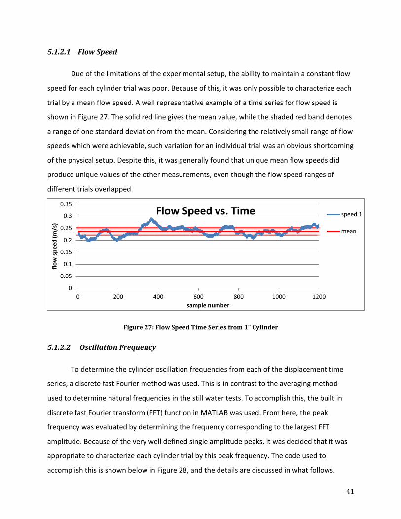
41
5.1.2.1 Flow Speed
Due of the limitations of the experimental setup, the ability to maintain a constant flow
speed for each cylinder trial was poor. Because of this, it was only possible to characterize each
trial by a mean flow speed. A well representative example of a time series for flow speed is
shown in Figure 27. The solid red line gives the mean value, while the shaded red band denotes
a range of one standard deviation from the mean. Considering the relatively small range of flow
speeds which were achievable, such variation for an individual trial was an obvious shortcoming
of the physical setup. Despite this, it was generally found that unique mean flow speeds did
produce unique values of the other measurements, even though the flow speed ranges of
different trials overlapped.
Figure 27: Flow Speed Time Series from 1" Cylinder
5.1.2.2 Oscillation Frequency
To determine the cylinder oscillation frequencies from each of the displacement time
series, a discrete fast Fourier method was used. This is in contrast to the averaging method
used to determine natural frequencies in the still water tests. To accomplish this, the built in
discrete fast Fourier transform (FFT) function in MATLAB was used. From here, the peak
frequency was evaluated by determining the frequency corresponding to the largest FFT
amplitude. Because of the very well defined single amplitude peaks, it was decided that it was
appropriate to characterize each cylinder trial by this peak frequency. The code used to
accomplish this is shown below in Figure 28, and the details are discussed in what follows.
0
0.05
0.1
0.15
0.2
0.25
0.3
0.35
0 200 400 600 800 1000 1200
flo
w s
pe
ed
(m
/s)
sample number
Flow Speed vs. Time speed 1
mean

42
The script is run for each individual data file generated from the experimental trials. The
variables v through z are then defined as vectors from the individual columns of the data file.
The period T is defined based on the user-input sampling rate (20 hz for most trials). A new
time vector t is then defined based on T and the sample length of the data file. The algorithm
requires that the signal have a number of data points equal to 2N, where N is an integer, so the
signal is padded with zero values to make it the appropriate length. A frequency vector f is then
defined based on half the sampling rate (Nyquist frequency), and the modified signal length.
From here, the single sided amplitude spectrum was plotted for evaluation, as seen in Figure
29. To determine peak frequency, the maximum value of the single sided amplitude is found
and the associated frequency returned. The previously added zero values cause a large
amplitude spectrum peak at a frequency near zero, so the determination of peak amplitude is
made starting from the 51st data point. This method effectively removes the influence of the
padded zero data.
importfile(input_file);
w = x0x22Acceleration0x22; v = x0x22Velocity0x22; y = x0x22Position0x22; x = x0x22Time0x22; z = x0x22FlowRate0x22;
T = 1/Fs; % Sample time L = length(y); % Length of signal t = (0:L-1)*T; % Time vector
NFFT = 2^nextpow2(L); % Next power of 2 from length of y Y = fft(y,NFFT)/L; f = Fs/2*linspace(0,1,NFFT/2+1);
% Plot single-sided amplitude spectrum. figure('visible','on'); plot(f,2*abs(Y(1:NFFT/2+1))); title(strcat(input_file,' - Single-Sided Amplitude Spectrum of y(t)')) xlabel('Frequency (Hz)') ylabel('|Y(f)|')
temp = 2*abs(Y(1:NFFT/2+1));
[max_val, peak_freq] = max(temp(51:end)); peak_freq = peak_freq + 50 ; % Adjust for removing first 50 values from temp peak_freq = f(peak_freq);
Figure 28: MATLAB FFT Script

43
Figure 29: 1.0" Cylinder Single Sided Amplitude Spectrum
1 2 3 4 5 6 7 8 90
0.005
0.01
0.015
0.02
2 4.csv - Single-Sided Amplitude Spectrum of y(t)
Frequency (Hz)
|Y(f
)|

44
5.1.2.3 Mean Amplitude
The mean cylinder oscillation amplitude over each time series was determined by
generating a phase portrait, or plot of velocity vs. position, for each data set. This method was
found to be far superior to individually determining each amplitude peak. A phase portrait
representative of most of the experimental data is shown by the blue trajectory in Figure 30.
Figure 30: 0.75" Cylinder Phase Portrait
The concentric rings can be thought of as being the path traced out as time elapses. As can be
seen, the locations near zero velocity correspond to peaks in the position value. This is intuitive,
since the cylinder should reach zero velocity at the peak of its oscillation. The dashed red lines
represent a region containing the lowest 10% of velocity values. The mean peak amplitude is
then found by evaluating the mean absolute value of the position data within this region. The
result is an amplitude reflective of the locations shown by the red circles.
-0.025 -0.02 -0.015 -0.01 -0.005 0 0.005 0.01 0.015 0.02 0.025
-0.25
-0.2
-0.15
-0.1
-0.05
0
0.05
0.1
0.15
0.2
0.25
position (m)
velo
city (
m/s
)

45
5.1.2.4 Potential Mechanical Power
The potential mechanical power transferred to the cylinders from the fluid was
experimentally determined using the same relations demonstrated in the modeling chapter.
The differential equation relating fluid force to cylinder behavior is given by Eq. 5-3.
Eq. 5-3
In this case, information for all the parameters and variables on the left side of the equation is
known from the experimental measurements and data. Using the experimental values along
with the cylinder oscillation data allowed the fluid force F(t) do be determined over each trial.
From there, F(t) was multiplied with the cylinder velocity data to produce a time series of
mechanical power P(t). Finally, the root mean square value of P(t), PRMS, was calculated to
produce a single metric for each cylinder trial, as given by Eq. 5-4.
√∑
Eq. 5-4
The parameter L is simply the length of the P(t) vector. Inherently, this representation of power
is slightly misleading, since it refers only to the power being transferred to the cylinder. Actual
extractable power, in the form of electricity generation, would necessarily be reduced by the
losses in the extraction process. Despite this, the power determined here provides a useful
baseline of the maximum potential power that could be extracted.
46
5.2 Results & Discussion
The final phase of this project consisted of interpretation and comparison of the
numerical results produced from the analysis described in section 5.1. The final data were
further reduced by attempting to collapse specific metrics from all cylinder trials onto single
plots, making use of the various non-dimensional parameters that were previously determined.
This section presents the final data plots that were determined to show meaningful or
significant trends. Additionally, this section provides an overall discussion of the observations
and findings made throughout the entire project, both quantitative and qualitative. As a note,
the data generated from the 1.25” cylinder was found to be unusable due to the fact that the
cylinder was reaching the shut height of the springs, seriously affecting the oscillations.
5.2.1 Oscillation frequency
All of the tests were performed at U* values between four and eight. According to lock-
in theory, the range of U* for which lock-in is most likely to occur is centered on a U* of five.
Although this was known a priori, it was not actively used in the experimental design process,
where the focus was on attempting to match cylinder natural frequency to predicted shedding
frequencies. However, significantly different experimental values of cylinder mass,
hydrodynamic mass, and flow speed were found compared to the values used in the initial
model.
One of the initial hopes of testing was to experimentally find the boundaries where VIV
ceases. In reality, limitations of the experimental set up resulted in test measurements entirely
within the ideal lock-in range. Due to this, it was not possible to determine the cutoff values of
U* for which no significant cylinder oscillation occurs. Despite this, the final comparison of
frequency to U* shown in Figure 31 has several interesting features.
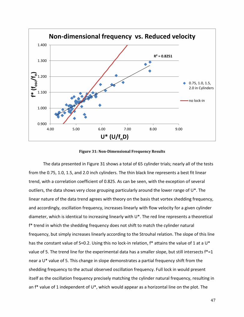
47
Figure 31: Non-Dimensional Frequency Results
The data presented in Figure 31 shows a total of 65 cylinder trials; nearly all of the tests
from the 0.75, 1.0, 1.5, and 2.0 inch cylinders. The thin black line represents a best fit linear
trend, with a correlation coefficient of 0.825. As can be seen, with the exception of several
outliers, the data shows very close grouping particularly around the lower range of U*. The
linear nature of the data trend agrees with theory on the basis that vortex shedding frequency,
and accordingly, oscillation frequency, increases linearly with flow velocity for a given cylinder
diameter, which is identical to increasing linearly with U*. The red line represents a theoretical
f* trend in which the shedding frequency does not shift to match the cylinder natural
frequency, but simply increases linearly according to the Strouhal relation. The slope of this line
has the constant value of S=0.2. Using this no lock-in relation, f* attains the value of 1 at a U*
value of 5. The trend line for the experimental data has a smaller slope, but still intersects f*=1
near a U* value of 5. This change in slope demonstrates a partial frequency shift from the
shedding frequency to the actual observed oscillation frequency. Full lock in would present
itself as the oscillation frequency precisely matching the cylinder natural frequency, resulting in
an f* value of 1 independent of U*, which would appear as a horizontal line on the plot. The
R² = 0.8251
0.900
1.000
1.100
1.200
1.300
1.400
4.00 5.00 6.00 7.00 8.00 9.00
f* (
f osc
/fn)
U* (U/fnD)
Non-dimensional frequency vs. Reduced velocity
0.75, 1.0, 1.5,2.0 in Cylinders
no lock-in

48
change in slope observed with respect to the no lock-in line towards a horizontal line signifies
that some frequency shift did occur. The margin of error throughout all the experimental
measurements could partially account for the discrepancies between full lock-in and the
experimental data, but overall the lack of complete lock-in is an inconclusive result. For this
reason, we recommend higher levels of precision and adjustability of the test set up for any
future work, as well as more realistic testing conditions.
5.2.2 Power Coefficient
A non-dimensionalized power coefficient was calculated for each of the valid
experiments. These were then plotted against the respective Reynolds Numbers, as shown in
Figure 32. The plot show that the power coefficient decays logarithmically with Reynolds
Number towards an asymptote at a power coefficient of 0.1. Ideally, the potential mechanical
power could be predicted based on this relationship, but given the disagreement between
theory and experimental data, it is unknown if this curve could be used to extrapolate for
values of Re far outside of this range.
Figure 32: Plot of Power Coefficients vs. Reynolds Number
0
0.1
0.2
0.3
0.4
0.5
0.6
0.0E+00 5.0E+03 1.0E+04 1.5E+04 2.0E+04
Cp
(P/
.5(1
/k)ρ
AU
3)
Re
Power Coefficient vs. Reynolds Number
0.75,1.0, 1.5,2.0 inCylinders

49
5.2.3 Power Harnessing Efficiency
The efficiency of the energy transfer from the fluid acting on the cylinders was plotted
against the respective reduced velocity U*, as shown in Figure 33. The peak efficiency was over
50% for the 0.75” cylinder. The efficiencies were lower for the larger cylinders and higher
velocities. The relationship between cylinder size and efficiency appears stronger than the
relationship between efficiency and velocity. The minimum efficiency was down to 10% for the
2 in cylinder at the maximum reduced velocity achieved. The length for all the cylinders was
constant. The relationship between the diameter of the cylinder to the length, or the aspect
ratio is 1:8.6 for the 0.75in cylinder. The aspect ratio is 1:3.8 for the 2in cylinder. These results
show that the efficiency is higher for slender cylinders. The VIVACE experiments had
determined that the ideal value for the aspect ratio is 1:8. Future experiments should test both
high and low aspect ratio cylinders to further develop an understanding between aspect ratio
and efficiency.
Figure 33: Power Efficiency vs. Reduced Velocity
0.00
0.10
0.20
0.30
0.40
0.50
0.60
3.00 4.00 5.00 6.00 7.00 8.00 9.00
η (
P/P
flu
id)
U* (U/fnD)
Power Efficiency vs. Reduced Velocity
0.75 in
1 in
1.5 in
2 in
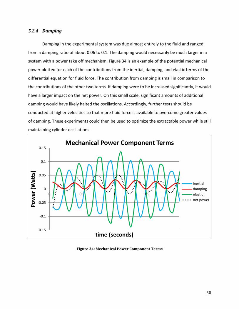
50
5.2.4 Damping
Damping in the experimental system was due almost entirely to the fluid and ranged
from a damping ratio of about 0.06 to 0.1. The damping would necessarily be much larger in a
system with a power take off mechanism. Figure 34 is an example of the potential mechanical
power plotted for each of the contributions from the inertial, damping, and elastic terms of the
differential equation for fluid force. The contribution from damping is small in comparison to
the contributions of the other two terms. If damping were to be increased significantly, it would
have a larger impact on the net power. On this small scale, significant amounts of additional
damping would have likely halted the oscillations. Accordingly, further tests should be
conducted at higher velocities so that more fluid force is available to overcome greater values
of damping. These experiments could then be used to optimize the extractable power while still
maintaining cylinder oscillations.
Figure 34: Mechanical Power Component Terms
-0.15
-0.1
-0.05
0
0.05
0.1
0.15
0 0.5 1 1.5 2
Po
we
r (W
atts
)
time (seconds)
Mechanical Power Component Terms
inertial
damping
elastic
net power
51
5.2.5 Hydrodynamic Mass
As discussed previously, the experimentally determined value for the added mass of a
cylinder was about 1.5 times greater on average than the theoretical values. The added mass
should be equal to the mass of the fluid volume displaced by the cylinder. The testing
conditions may have contributed to this difference. The small gap between the cylinder and the
surroundings of the cross-section may have increased the inertia needed to displace the
volume of the fluid. Future experiments should have a larger gap between the cylinder and the
boundaries to limit the effects on added mass. Since most calculations were based on the
experimentally determined added mass, the same experiments conducted under different test
setups would have different end results. Ensuring that the experimental added mass closely
matches the theoretical added mass for all future experiments would allow for more accurate
comparisons between experiments.

52
5.2.6 Power Density
Assuming set distances between cylinders in a power plant array, power density,
modeled in Figure 35 below, the power density of the array can be calculated as a function of
cylinder diameter. Distances t and p shown below are linear functions of diameter.
Figure 35: Power Density Schematic
VIVACE proposes the staggered cylinder arrangement from Figure 35 based on
relationships of t and p shown in Eq. 5-5 and Eq. 5-6 below.
Eq. 5-5
Eq. 5-6
The number of cylinders and resulting volume (V(D) )of the array can be calculated using
Eq. 5-7 and Eq. 5-8 below, where a is the number of cylinders deep in flow direction, b is the
number of cylinders tall, and c is the number of a x b arrays into the page.
Eq. 5-7
[ ] [ ] Eq. 5-8
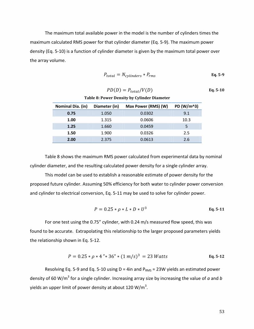
53
The maximum total available power in the model is the number of cylinders times the
maximum calculated RMS power for that cylinder diameter (Eq. 5-9). The maximum power
density (Eq. 5-10) is a function of cylinder diameter is given by the maximum total power over
the array volume.
Eq. 5-9
Eq. 5-10
Table 8: Power Density by Cylinder Diameter
Nominal Dia. (in) Diameter (in) Max Power (RMS) (W) PD (W/m^3)
0.75 1.050 0.0302 9.1
1.00 1.315 0.0606 10.3
1.25 1.660 0.0459 5
1.50 1.900 0.0326 2.5
2.00 2.375 0.0613 2.6
Table 8 shows the maximum RMS power calculated from experimental data by nominal
cylinder diameter, and the resulting calculated power density for a single cylinder array.
This model can be used to establish a reasonable estimate of power density for the
proposed future cylinder. Assuming 50% efficiency for both water to cylinder power conversion
and cylinder to electrical conversion, Eq. 5-11 may be used to solve for cylinder power.
Eq. 5-11
For one test using the 0.75” cylinder, with 0.24 m/s measured flow speed, this was
found to be accurate. Extrapolating this relationship to the larger proposed parameters yields
the relationship shown in Eq. 5-12.
Eq. 5-12
Resolving Eq. 5-9 and Eq. 5-10 using D = 4in and PRMS = 23W yields an estimated power
density of 60 W/m3 for a single cylinder. Increasing array size by increasing the value of a and b
yields an upper limit of power density at about 120 W/m3.
54
5.2.7 Cylinder Amplitude
It was found that cylinder amplitude generally increased with an increase in flow speed.
According to existing theory, amplitudes in the range of 1-2 diameters are reasonable; however
our experiments never resulted in amplitude above 1 diameter. This result is likely influenced
by the scale of the experimental set up. First, flow velocities used in this experiment are in the
lower range of VIV inducing speeds. Increasing the flow velocity to a velocity range of 1-3 m/s
as recommended for future testing may yield higher amplitude vibration. Also, amplitude may
have been limited by the small range of available space for the cylinder to vibrate. The
extension springs used in this experiment were seen on a few occasions to reach shut length.
Linear stiffness range for springs should generally be assumed to be from 15-85% of spring
extension. Stiffness varies nonlinearly outside this range, and for this small scale experiment,
the change in stiffness may have affected the overall amplitude.
A limitation of the mathematical model is that the estimate for cylinder vibration
amplitude did not take the self-limiting effect into account. This seemed a reasonable
assumption during the mathematical modeling stages of the project, but came into question
after compiling the test data. As a result, experimental findings range both above and below
the model predictions for maximum cylinder amplitude.
To compensate for these deviations in experimental results from VIV theory, the future
testing set up design has been based on the theoretical maximum amplitude over diameter
ratio (2.5-3). It is expected that in a more robust future test model, testing data will more
closely agree with theory.

55
5.2.8 Observations
It was observed while testing that placing one’s hand 2 or 3 inches in front of the
cylinder did not significantly inhibit vibration of the cylinder. It was also estimated that the
force of the cylinder pushing up on one’s hand while an object was 2 or 3 inches in front of the
cylinder remained about the same. This leads us to believe that aquatic obstructions, either
wildlife or debris that enter the path of water over the cylinder, will not have a significant effect
on the vibration.
It was also seen through comparison of flow velocity to cylinder position, velocity, and
acceleration data that measured spikes in the flow velocity did not result in quantifiable
changes in the cylinder oscillation frequency. There are a few possible reasons for this. First,
resolution of the flow rate sensor was 1.2 mm/s. Also, a limitation of measuring with the flow
rate sensor and displacement sensor simultaneously was that a uniform sampling frequency
needed to be specified. The recommended sampling frequency for the flow sensor was 4 Hz, up
to 50 Hz for the displacement sensor, while 20 or 30 Hz was used during the experiment.

56
6 Recommendations for Future Work
This section outlines potential future work to be done in a continuation of this project.
Design of future test set up is discussed as well as experiments to be conducted.
6.1 Project Continuation Proposal
The previously discussed experiments were conducted at flow speeds up to
approximately 0.35m/s. These speeds are significantly lower than those found in ocean
currents and river flows. Increasing the Reynolds number by increasing fluid velocity by an
order of magnitude to 1-3 m/s, and increasing cylinder diameter by a few inches would allow
for results that could more accurately predict the potential for the technology under realistic
conditions. Because of the low velocity for the fluid in the initial experiment, the lift force of the
fluid acting on the cylinders was also small. This lift force could only overcome small amounts of
damping and so damping was limited to the damping caused by the fluid. The vibrations of the
cylinders subjected to fluid flow can only perform useful work if a system exists to extract the
energy. Any power take off system would significantly increase the damping of the setup. The
lift force of the fluid acting on the cylinder is dependent on the velocity of the fluid squared.
Thus increasing the fluid velocity by an order of magnitude would increase the lift force by a
factor of 100. This larger lift force would be able to overcome the damping introduced by a
power take off mechanism and would allow for experiments that can truly test the potential for
power generation.
It is proposed that future participants in this project area assess the possibility of use of
large scale test facilities such as those at the Alden Research Laboratory. The Alden Research
Laboratory in Holden, MA is the oldest continuously run hydro research facility in the United
States. The company prides itself on using its resources to support the future of clean,
renewable hydro energy. Numerous test flumes and tanks exist at the site for the testing and
optimization of hydrokinetic equipment. Many of these facilities are capable of testing
prototype turbines at full scale operating velocities. The company’s newest flume has a test
section of 80x20x10 feet with a flow rate of 500 cubic feet per second. With guide walls, the

57
flow can be channeled to produce velocities up to 10ft/s or 3m/s. The flume functions similarly
to the flow tank developed for the discussed experiments, but on a much larger scale. The
flume is a closed loop, two-level system that incorporates twin axial flow pumps to generate a
flow through the test section. A schematic of the flume is shown in Figure 36.
Figure 36: Schematic of the Alden Labs Test Flume
These facilities provide greater flow speeds with greater control than the testing setup
used in the discussed experiments. The use of such testing conditions would increase the
flexibility of future experiments and lead to a better understanding of the potential for vortex
induced vibrations as a source for clean energy.
6.2 Task Specifications
Under the new proposed testing conditions, a new test rig will need to be designed.
Below is an initial list of some of the recommended task specifications.
1. Device must accommodate the installation and data measurement of
interchangeable cylinders, or other geometry, 1 meter in length.
An important component of future testing in this area is the addition or simulation of a
power take off system. Both methods introduce a larger amount of damping into the total
force acting on the cylinder. One way to increase the amount of damping the system can
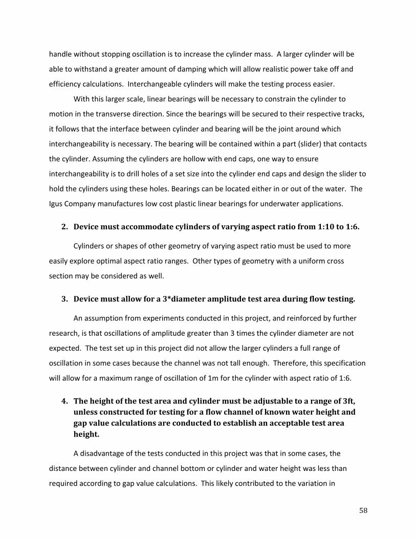
58
handle without stopping oscillation is to increase the cylinder mass. A larger cylinder will be
able to withstand a greater amount of damping which will allow realistic power take off and
efficiency calculations. Interchangeable cylinders will make the testing process easier.
With this larger scale, linear bearings will be necessary to constrain the cylinder to
motion in the transverse direction. Since the bearings will be secured to their respective tracks,
it follows that the interface between cylinder and bearing will be the joint around which
interchangeability is necessary. The bearing will be contained within a part (slider) that contacts
the cylinder. Assuming the cylinders are hollow with end caps, one way to ensure
interchangeability is to drill holes of a set size into the cylinder end caps and design the slider to
hold the cylinders using these holes. Bearings can be located either in or out of the water. The
Igus Company manufactures low cost plastic linear bearings for underwater applications.
2. Device must accommodate cylinders of varying aspect ratio from 1:10 to 1:6.
Cylinders or shapes of other geometry of varying aspect ratio must be used to more
easily explore optimal aspect ratio ranges. Other types of geometry with a uniform cross
section may be considered as well.
3. Device must allow for a 3*diameter amplitude test area during flow testing.
An assumption from experiments conducted in this project, and reinforced by further
research, is that oscillations of amplitude greater than 3 times the cylinder diameter are not
expected. The test set up in this project did not allow the larger cylinders a full range of
oscillation in some cases because the channel was not tall enough. Therefore, this specification
will allow for a maximum range of oscillation of 1m for the cylinder with aspect ratio of 1:6.
4. The height of the test area and cylinder must be adjustable to a range of 3ft,
unless constructed for testing for a flow channel of known water height and
gap value calculations are conducted to establish an acceptable test area
height.
A disadvantage of the tests conducted in this project was that in some cases, the
distance between cylinder and channel bottom or cylinder and water height was less than
required according to gap value calculations. This likely contributed to the variation in

59
apparent mass calculations. To accurately analyze a cylinder of given mass, these calculations
should be accounted for.
5. In addition to the mass of the cylinders, the mass of the testing rig will not
exceed 10kg.
The force of lift would be significantly greater at the high velocities. Nevertheless, if the
mass of the test rig is too great, the force will not be strong enough to force the setup to
oscillate. This mass includes end caps for the cylinders, sensors, springs, and the frame used to
hold the cylinder. It does not include the hydrodynamic mass of the cylinder or the mass of the
cylinder itself. Thus, this value should be constant for all experiments independent of the
cylinder size. The maximum force of lift for these cylinder sizes and flow speeds in the lock-in
range will be approximately 40-130N.
6. The stiffness of all springs storing cylinder energy must be adjustable.
As a result the limit of cylinder size and flow speed in the test set up in this project, only
a small range of spring stiffness was available to provide lock-in, and stiffness was not
adjustable. Adjustable spring stiffness in this device will enable easier testing at a wider range
of mass and other parameters. The range for the total stiffness of the system is 4000N/m to
7000N/m. The formula
where k is stiffness, G is the shear modulus, d is the wire diameter, D is the outer diameter and
N is the number of active coils, provides an approximation for the stiffness of a spring. Reducing
the number of active coils will increase the stiffness of the spring. This will allow for the same
spring to provide multiple values of stiffness. A compression spring could be screwed onto a
threaded bolt with the correct pitch and diameter to reduce the number of active coils and
increase the stiffness. To achieve the listed specification, each spring will need a stiffness of
2000N/m. The shear modulus for steel is approximately 80 Gpa. A spring with a diameter of
0.01m and wire diameter of 0.0012m will have 13 coils. From the McMaster-Carr Catalog, a
spring with these specifications is available with a length of 0.076m. Reducing the active

60
number of coils to 7 would achieve the max stiffness of 3500N/m I each spring. Many spring
manufacturers will create custom springs based on requirements for length, pitch, stiffness,
and diameter. A longer spring would be needed to accommodate the amplitude of oscillations.
7. The damping of all dampers affecting cylinder motion during testing must be
adjustable.
Adjustable damping is critical to the available power optimization testing. Damping
must be optimized with cylinder oscillation and must be high to simulate power extraction but
not so high as to critically interfere with the vibrations. In future testing, this relationship must
be tested and established.
8. The device must be compatible with one or more high resolution or analog
linear displacement sensors.
A disadvantage of tests conducted in this project was sensor resolution. To avoid
resolution issues, an analog sensor such as a linear variable differential transformer (LVDT)
could be used, which converts linear motion to a signal using the motion of a magnet over a
coil.
Stellar Technology Inc. offers the LLC65X, a 37 inch stroke linear displacement LVDT,
which matches the absolute maximum displacement range required according to Task
Specification 3. Different LVDTs are available for either out of water or underwater use.
9. The cylinders will be Schedule 10 aluminum pipes.
PVC pipes for the proposed sizes for the cylinders are too light to achieve the proper
natural frequencies for lock-in. Aluminum pipes will provide a suitable mass that is not too
great for the lift force of the fluid acting on the cylinders.

61
6.3 Design Concepts
This section outlines a few conceptual designs. The part views in Figure 37 show the
slider concept design.
Figure 37: Slider Concept Design
In this design, the large center hole is to hold a linear bearing. The two adjacent holes provide a
location to secure the ends of a spring and a damper. The circular protrusion will be secured to
the block by a bolt. The bolt hole in the block will be counter bored, as shown in Figure 38
below.
Figure 38: Right View of Slider Concept
The circular protrusion will be inserted into a hole in the end of a cylinder for a firm fit.
For tests with aluminum pipes, this protrusion can be bolted into the appropriate sized end
caps pressed onto either side of the cylinder. The guides for the linear bearings will be attached
to a stationary frame. This frame will need to be secured within the testing cross section. This
frame will hold a LVDT sensor above the cylinder. The core of the LVDT will be attached directly
to the cylinder so that it will move in conjunction with the displacement of the cylinder.

62
6.4 Suggested Experiments
As previously discussed, testing facilities such as those at Alden Labs would increase the
flexibility of future experiments. Based on the new testing rig, a series of new experiments are
proposed below. These values are based on the mathematical model discussed in Chapter 3. In
addition to allowing for a test rig with much higher values of damping, the new facilities will
allow for tests that occur both outside and within the lock-in ranges. A much greater range of
Reynolds numbers can also be achieved to further develop the relationship between flow
conditions and power.
Experiment 1
The length of the cylinder is a constant length of 1m and the damping will have a
constant value. A range of cylinder diameters are chosen to achieve aspect ratios from 1:6 to
1:10. The stiffness of each setup is chosen so that a 1:1 ratio of vortex shedding frequency to
natural frequency will occur at an approximate flow speed of 1.5 m/s. The natural frequency
calculation uses the mass of the cylinder with the hydrodynamic mass and the mass of the rest
of the test rig. The test rig is assumed to have a mass of 10kg, its maximum based on the task
specifications. With flow speeds of approximately below 1 m/s or above 1.8m/s, the system will
be outside of the theoretical +/-30% lock-in region. For each cylinder, the flow velocity will be
adjusted at constant intervals from 0m/s to 2m/s. At each interval, the displacement of the
cylinder will be recorded for 60 seconds. This will allow for data that will show the difference in
amplitude, frequency, power, and efficiency of the cylinder within the lock-in range and outside
of the lock-in range. By comparing these same results between the varying cylinders, the
relationship between aspect ratio and efficiency can be further explored. Additionally, these
results can be used to create a non-dimensional curve to plot the relationship between the
power coefficient and the Reynolds Number. This experiment can be repeated with different
stiffness values to create a different natural frequency for each of the cylinders tested.
Additional cylinder sizes could also be used.
63
Table 9: Proposed Setups for Testing the Lock-in Range
Aspect Ratio Diameter Cylinder Mass Stiffness
1:6 6in/0.15m 4.1kg 4000N/m 1:7 5in/0.13m 3.4kg 4500N/m 1:8 4.5in/0.11m 3.0kg 5000N/m 1:9 4in/0.10m 2.7kg 6000N/m
1:10 3in/0.90m 2.3kg 7000N/m
Experiment 2
This experiment will explore the relationship between damping and the oscillations of
the cylinders. The same cylinders and same values of stiffness from the previous experiment
can be used. The velocity for each test is held constant at 1m/s so that the cylinders will
oscillate within the lock-in region. The damping ratio of the cylinders will be adjusted at
constant intervals between the minimum value and the maximum value achievable by the test
setup. For each damping ratio, the displacement of the cylinder will be recorded for 60 seconds.
These tests will show the relationship between the damping of the system and the ability of the
system to oscillate. The objective of this portion of the testing schedule is to determine what
the ideal value of zeta is, or at what value the most power can be extracted from the cylinder
without critically interfering with cylinder oscillations.
64
7 Conclusions
Through mathematical modeling and small-scale experiments, the potential for vortex-
induced vibrations as an energy source was studied. Initial research was conducted on VIV
theory and existing aquatic energy technologies, including VIVACE. Based on the background
research, a mathematical model was created in order to predict the relationship between
experimental parameters and cylinder response, to establish feasibility of small scale VIV
testing and to create estimates for experimental results. Measured oscillation frequencies were
generally in-between the measured natural frequency and the theoretically calculated shedding
frequency. Because the oscillation frequencies did not match the natural frequencies, the
systems were likely not fully locked- in. But because the ratio of natural frequency to oscillation
frequency was consistently less than the calculated ratio of shedding frequency to the
oscillation frequency, the lock-in conditions had an impact on the dynamic behavior of the
cylinders. Cylinder amplitude estimates proved accurate in some cases. However, the equation
for amplitude in the model is linear, whereas VIV is known to be highly non-linear.
A test set up was designed and constructed using purchased hardware, hand
construction and CNC machining processes. Throughout the building and testing phases of the
project, possible improvements to the set up became apparent, such as adjustable stiffness and
damping. Through the use of this test set up, still water tests were conducted to measure the
natural frequency of each cylinder, establish damping ratios, and to determine the
hydrodynamic mass of the cylinders. Flowing water tests were then conducted to measure the
displacement, velocity, and acceleration of the cylinder at various flow velocities. Tests were
limited in scope, precision, and accuracy due to lack of control of flow velocity and the limited
resolution of the device used to measure displacement. The motion sensor had a resolution of
1mm. This created large uncertainty for damping ratio results because the logarithmic decay
was on the scale of millimeters. Because damping was a small contribution to the power
equation, this did not significantly impact the uncertainty in power calculations. If future
experiments were conducted with greater damping values, damping would need to be
measured with higher resolution devices. The resolution of the LVDT displacement sensor
would only be limited by noise in the signal conditioner and by the resolution of the output

65
device. This would allow for lower uncertainty values for calculated parameters such as
damping. Because of the limited scope, all tests were within the lock-in range. None of the
experiments were able to test the changes in oscillation behavior below or above lock-in.
The experimentally determined parameters were used with the differential equation of
motion for the cylinders to calculate the force of lift with respect to time and ultimately
calculate the power transferred from the fluid. From this data, a curve relating power to flow
conditions was plotted and showed that the non-dimensional power term decreased
logarithmically with Reynolds number. This curve could be used to predict power based on
known conditions. Due to the inconsistencies between theoretical and observed added mass,
this curve would only be valid for this test setup. Future experiments should continue to
explore this relationship under different conditions. Additionally, the cylinder with aspect ratio
of 1:8.6 showed efficiencies around 50% while the cylinder with the aspect ratio of 1:3.8
showed that the efficiency dropped to around 15%. This suggests that slender bodies will
provide more efficient power extraction. However, the results showed increases in the
magnitude of power with increased cylinder size. Future tests should be conducted to
determine the aspect ratio that will optimize efficiency.
Overall, this project demonstrated proof of concept for scale VIV tests. At this small
scale, the maximum calculated power ranged from 15 to 45 mili-watts RMS and a maximum
power density of 10.3 watts/m3. Based on lessons from this project, design of a further testing
set up and a testing plan have been presented for larger scale VIV tests. The power density
model showed that single cylinder power density of 60 watts per cubic meter for a 4 inch
diameter, 36 inch long cylinder is feasible. These tests would allow for a greater force to
overcome damping caused by a power-take off system. By incorporating a power take off
system into future experiments, the validity of the analytical power calculations could be tested
and true data for extractable power can be measured. Because the results showed the
phenomenon occurring at flow velocities lower than the realistic conditions, the potential exists
for vortex induced vibrations as a source of energy generation.
66
8 References
1. Bernitsas. (2009). The VIVACE Converter: Model Tests at High Damping and Reynolds
Number Around 105. Journal of Offshore Mechanics and Arctic Engineering, 12.
2. Bernitsas, M. M., Raghavan, K., Ben-Simon, Y., & Garcia, E. M. (2008). VIVACE (Vortex
Induced Vibration Aquatic Clean Energy): A New Concept in Generation of Clean and
Renewable Energy From Fluid Flow. Journal of Offshore Mechanics and Arctic
Engineering.
3. Blevins. (1990). Flow-Induced Vibration. New York: Van Nostrand Reinhold.
4. Govardhan, C. a. (2004). VORTEX-INDUCED VIBRATIONS. Annual Review of Fluid
Mechanics, (p. 53).
5. MIT. (n.d.). Retrieved 10 2010, from Open Course Ware.
6. Raghavan, K., Bernitsas, M. M., & Maroulis, D. E. (2009). Effect of Bottom Boundary on
VIV for Energy Harnessing at 8E3<Re<1.5E5. Journal of Offshore Mechanics and Arctic
Engineering.

67
Appendix A Still Water Decay Test Data
mass (gr) zeta 1 zeta 2 frequency (hz)
135 0.093 0.081 1.770
135 0.128 0.046 1.900
135 0.093 0.081 1.820
135 0.128 0.046 1.860
135 0.093 0.081 1.950
mean 0.107 0.067 1.860
152 0.064 0.046 1.820
152 0.064 0.046 1.760
152 0.072 0.025 1.820
152 0.064 0.046 1.790
152 0.072 0.025 1.820
mean 0.067 0.038 1.802
Table 10: Data Summary of 0.75" Cylinder
mass (gr) zeta 1 zeta 2 frequency (hz)
155 0.077 0.046 1.600
155 0.064 0.046 1.589
155 0.077 0.046 1.600
155 0.058 0.064 1.600
155 0.058 0.064 1.600
mean 0.067 0.053 1.598
172 0.070 0.064 1.589
172 0.058 0.064 1.579
172 0.058 0.064 1.589
172 0.070 0.064 1.579
172 0.077 0.046 1.600
mean 0.067 0.061 1.587
Table 11: Data Summary of 1" Cylinder
mass (gr) zeta 1 zeta 2 frequency (hz)
272 0.046 0.029 1.170
272 0.055 0.014 1.180
272 0.075 reject 1.180
272 0.060 0.015 reject
272 0.064 0.017 1.150
mean 0.060 0.019 1.170
289 0.055 0.014 1.140
289 0.055 0.014 1.150
289 0.055 0.014 1.130
289 0.043 0.027 1.130
289 0.052 0.013 1.140
mean 0.052 0.016 1.138
Table 12: Data Summary of 1.5" Cylinder
mass (gr) zeta 1 zeta 2 frequency (hz)
343 0.051 0.034 0.690
343 0.053 0.026 0.690
343 0.053 0.035 0.690
343 0.053 0.035 0.680
343 0.051 0.043 0.690
mean 0.052 0.035 0.688
377 0.041 0.031 0.678
377 0.058 0.029 0.678
377 0.048 0.031 0.678
377 0.055 0.031 0.690
377 0.048 0.031 0.690
mean 0.050 0.031 0.683
Table 13: Data Summary of 2" Cylinder

68
Appendix B Flowing Water Test Data
Tables 14: 0.75" Cylinder Final Data
trial 1 2 3 4
m cyl (kg) 0.104 0.121 0.138 0.155
m tot (kg) 0.317 0.334 0.351 0.374
m* 0.488 0.568 0.648 0.708
d (m) 0.0267 0.0267 0.0267 0.0267
k (N/m) 47.6 47.6 47.6 47.6
Zeta 0.11 0.11 0.11 0.11
fn water (hz) 1.950 1.900 1.860 1.802
L (m) 0.22 0.22 0.22 0.22 Trial 1
mean flow(m/s) SD % f shd (hz) f osc (hz) osc/shd f* X mean (m) Prms (W) U* η Cp Re A/D
0.250 7.0 1.850 1.919 1.037 0.984 0.013 0.0169 4.791 0.37 0.37 5.09E+03 0.49
0.246 6.8 1.822 1.978 1.085 1.014 0.016 0.0213 4.718 0.49 0.49 5.01E+03 0.60
0.251 6.6 1.862 1.963 1.054 1.006 0.016 0.0213 4.822 0.46 0.46 5.12E+03 0.60
0.273 9.7 2.022 2.095 1.036 1.074 0.018 0.0272 5.235 0.46 0.46 5.56E+03 0.67
0.301 5.8 2.234 2.124 0.951 1.089 0.018 0.0302 5.784 0.38 0.38 6.14E+03 0.67
mean 7.2
0.43 0.43
0.61 Trial 2
mean flow(m/s) SD % f shd (hz) f osc (hz) osc/shd f* X mean (m) Prms (W) U* η Cp Re A/D
0.243 6.5 1.805 1.904 1.055 1.002 0.013 0.0186 4.798 0.44 0.44 4.96E+03 0.49
0.265 7.8 1.964 1.919 0.977 1.010 0.016 0.0221 5.222 0.41 0.41 5.40E+03 0.60
0.242 6.6 1.794 1.934 1.078 1.018 0.016 0.0216 4.768 0.52 0.52 4.93E+03 0.60
0.253 7.2 1.874 1.978 1.055 1.041 0.017 0.0244 4.981 0.52 0.52 5.15E+03 0.64
0.293 6.6 2.172 2.036 0.937 1.072 0.018 0.0285 5.774 0.39 0.39 5.97E+03 0.67
mean 6.9
0.45 0.45
0.60 Trial 3
mean flow(m/s) SD % f shd (hz) f osc (hz) osc/shd f* X mean (m) Prms (W) U* η Cp Re A/D
0.240 6.7 1.778 1.885 1.060 1.013 0.015 0.0193 4.829 0.48 0.48 4.89E+03 0.56
0.240 10.0 1.776 1.875 1.056 1.008 0.016 0.0213 4.823 0.53 0.53 4.88E+03 0.60
0.264 8.6 1.954 1.943 0.995 1.045 0.017 0.0229 5.306 0.43 0.43 5.37E+03 0.64
0.266 8.6 1.973 1.973 1.000 1.061 0.017 0.0246 5.356 0.45 0.45 5.42E+03 0.64
0.281 8.5 2.084 2.041 0.979 1.097 0.018 0.0277 5.658 0.43 0.43 5.73E+03 0.67
mean 8.5
0.46 0.46
0.62 Trial 4
mean flow(m/s) SD % f shd (hz) f osc (hz) osc/shd f* X mean (m) Prms (W) U* η Cp Re A/D
0.246 8.5 1.823 1.865 1.023 1.035 0.016 0.0201 5.109 0.46 0.46 5.01E+03 0.60
0.247 5.5 1.832 1.875 1.024 1.041 0.017 0.022 5.134 0.50 0.50 5.03E+03 0.64
0.240 6.6 1.781 1.885 1.058 1.046 0.016 0.0214 4.992 0.53 0.53 4.90E+03 0.60
0.277 5.2 2.056 1.943 0.945 1.078 0.017 0.0247 5.761 0.40 0.40 5.65E+03 0.64
0.296 5.0 2.193 2.002 0.913 1.111 0.018 0.0265 6.146 0.35 0.35 6.03E+03 0.67
mean 6.2
0.45 0.45
0.63

69
Tables 15: 1" Cylinder final Data
trial 1 2 3 4
m cyl (kg) 0.158 0.175 0.192 0.209
m tot (kg) 0.475 0.482 0.502 0.519
m* 0.498 0.571 0.619 0.674
d (m) 0.0334 0.0334 0.0334 0.0334
k (N/m) 47.6 47.6 47.6 47.6
Zeta 0.067 0.067 0.067 0.067
fn water (hz) 1.60 1.59 1.55 1.52
L (m) 0.22 0.22 0.22 0.22
Trial 1
mean flow(m/s) SD % f shd (hz) f osc (hz) osc/shd f* X mean (m) Prms (W) U* η Cp Re A/D
0.247 8.9 1.462 1.631 1.115 1.021 0.011 0.0176 4.622 0.32 0.32 6.29E+03 0.33
0.256 9.7 1.516 1.553 1.024 0.972 0.014 0.0158 4.793 0.26 0.26 6.52E+03 0.42
0.258 7.6 1.531 1.699 1.110 1.063 0.018 0.0199 4.838 0.32 0.32 6.58E+03 0.54
0.272 8.8 1.614 1.690 1.047 1.057 0.019 0.0202 5.100 0.27 0.27 6.94E+03 0.57
0.293 6.6 1.737 1.709 0.984 1.069 0.020 0.0207 5.490 0.22 0.22 7.47E+03 0.60
mean 8.3
0.28 0.28
0.49
Trial 2
mean flow(m/s) SD % f shd (hz) f osc (hz) osc/shd f* X mean (m) Prms (W) U* η Cp Re A/D
0.237 7.6 1.403 1.514 1.079 0.954 0.011 0.0154 4.466 0.32 0.32 6.03E+03 0.31
0.238 6.2 1.410 1.572 1.115 0.991 0.018 0.0199 4.486 0.40 0.40 6.06E+03 0.52
0.261 6.7 1.549 1.611 1.040 1.015 0.020 0.0226 4.930 0.35 0.35 6.66E+03 0.60
0.274 5.6 1.625 1.650 1.015 1.040 0.022 0.0252 5.173 0.33 0.33 6.99E+03 0.66
0.282 3.9 1.669 1.680 1.006 1.058 0.022 0.0247 5.313 0.30 0.30 7.18E+03 0.66
mean 6.0
0.34 0.34
0.55
Trial 3
mean flow(m/s) SD % f shd (hz) f osc (hz) osc/shd f* X mean (m) Prms (W) U* η Cp Re A/D
0.223 8.8 1.323 1.494 1.129 0.964 0.015 0.0144 4.312 0.35 0.35 5.69E+03 0.45
0.251 8.1 1.489 1.543 1.037 0.996 0.018 0.0194 4.851 0.33 0.33 6.40E+03 0.54
0.262 6.2 1.554 1.611 1.037 1.040
0.0241 5.065 0.36 0.36 6.69E+03 0.00
0.270 8.8 1.600 1.611 1.007 1.040 0.021 0.0233 5.214 0.32 0.32 6.88E+03 0.63
0.284 6.6 1.681 1.641 0.976 1.059 0.023 0.025 5.477 0.30 0.30 7.23E+03 0.69
mean 7.7
0.33 0.33
0.46
Trial 4
mean flow(m/s) SD % f shd (hz) f osc (hz) osc/shd f* X mean (m) Prms (W) U* η Cp Re A/D
0.221 9.5 1.312 1.484 1.131 0.974 0.016 0.015 4.347 0.38 0.38 5.64E+03 0.48
0.240 8.5 1.422 1.514 1.064 0.993 0.018 0.0193 4.712 0.38 0.38 6.12E+03 0.54
0.255 8.8 1.509 1.572 1.042 1.032 0.022 0.0223 4.999 0.37 0.37 6.49E+03 0.66
0.281 5.7 1.666 1.621 0.973 1.064 0.023 0.0257 5.520 0.32 0.32 7.16E+03 0.69
0.285 5.8 1.691 1.631 0.965 1.070 0.024 0.0274 5.602 0.32 0.32 7.27E+03 0.72
mean 7.7
0.35 0.35
0.62
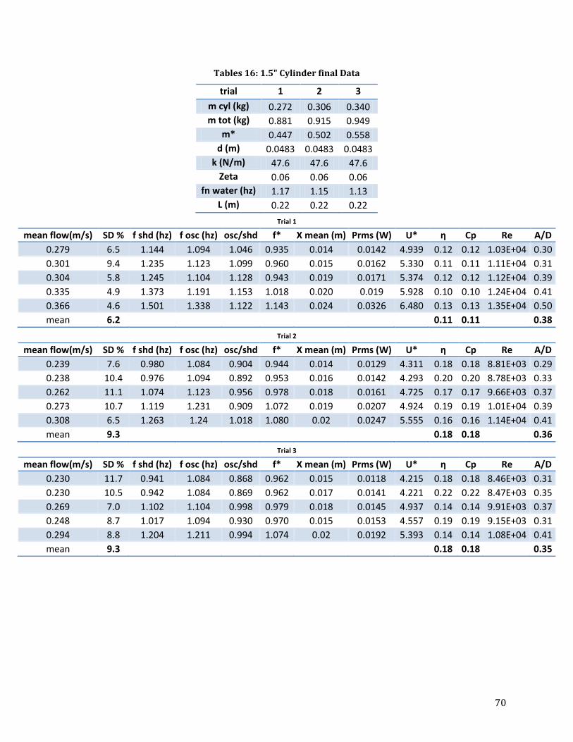
70
Tables 16: 1.5" Cylinder final Data
trial 1 2 3
m cyl (kg) 0.272 0.306 0.340
m tot (kg) 0.881 0.915 0.949
m* 0.447 0.502 0.558
d (m) 0.0483 0.0483 0.0483
k (N/m) 47.6 47.6 47.6
Zeta 0.06 0.06 0.06
fn water (hz) 1.17 1.15 1.13
L (m) 0.22 0.22 0.22
Trial 1
mean flow(m/s) SD % f shd (hz) f osc (hz) osc/shd f* X mean (m) Prms (W) U* η Cp Re A/D
0.279 6.5 1.144 1.094 1.046 0.935 0.014 0.0142 4.939 0.12 0.12 1.03E+04 0.30
0.301 9.4 1.235 1.123 1.099 0.960 0.015 0.0162 5.330 0.11 0.11 1.11E+04 0.31
0.304 5.8 1.245 1.104 1.128 0.943 0.019 0.0171 5.374 0.12 0.12 1.12E+04 0.39
0.335 4.9 1.373 1.191 1.153 1.018 0.020 0.019 5.928 0.10 0.10 1.24E+04 0.41
0.366 4.6 1.501 1.338 1.122 1.143 0.024 0.0326 6.480 0.13 0.13 1.35E+04 0.50
mean 6.2
0.11 0.11
0.38
Trial 2
mean flow(m/s) SD % f shd (hz) f osc (hz) osc/shd f* X mean (m) Prms (W) U* η Cp Re A/D
0.239 7.6 0.980 1.084 0.904 0.944 0.014 0.0129 4.311 0.18 0.18 8.81E+03 0.29
0.238 10.4 0.976 1.094 0.892 0.953 0.016 0.0142 4.293 0.20 0.20 8.78E+03 0.33
0.262 11.1 1.074 1.123 0.956 0.978 0.018 0.0161 4.725 0.17 0.17 9.66E+03 0.37
0.273 10.7 1.119 1.231 0.909 1.072 0.019 0.0207 4.924 0.19 0.19 1.01E+04 0.39
0.308 6.5 1.263 1.24 1.018 1.080 0.02 0.0247 5.555 0.16 0.16 1.14E+04 0.41
mean 9.3
0.18 0.18
0.36
Trial 3
mean flow(m/s) SD % f shd (hz) f osc (hz) osc/shd f* X mean (m) Prms (W) U* η Cp Re A/D
0.230 11.7 0.941 1.084 0.868 0.962 0.015 0.0118 4.215 0.18 0.18 8.46E+03 0.31
0.230 10.5 0.942 1.084 0.869 0.962 0.017 0.0141 4.221 0.22 0.22 8.47E+03 0.35
0.269 7.0 1.102 1.104 0.998 0.979 0.018 0.0145 4.937 0.14 0.14 9.91E+03 0.37
0.248 8.7 1.017 1.094 0.930 0.970 0.015 0.0153 4.557 0.19 0.19 9.15E+03 0.31
0.294 8.8 1.204 1.211 0.994 1.074 0.02 0.0192 5.393 0.14 0.14 1.08E+04 0.41
mean 9.3
0.18 0.18
0.35

71
Tables 17: 2" Cylinder final Data
trial 1 2
m cyl (kg) 0.337 0.405
m tot (kg) 1.267 1.335
m* 0.362 0.435
d (m) 0.060 0.060
k (N/m) 23.8 23.8
Zeta 0.052 0.052
fn water (hz) 0.688 0.672
L (m) 0.22 0.22
Trial 1
mean flow(m/s) SD % f shd (hz) f osc (hz) osc/shd f* X mean (m) Prms (W) U* η Cp Re A/D
0.215 12.1 0.704 0.752 0.937 1.093 0.036 0.0247 5.170 0.38 0.38 9.87E+03 0.60
0.247 9.6 0.811 0.791 1.025 1.150 0.039 0.0317 5.951 0.32 0.32 1.14E+04 0.65
0.272 9.3 0.894 0.830 1.078 1.207 0.033 0.0395 6.566 0.30 0.30 1.25E+04 0.55
0.320 5.4 1.049 0.879 1.194 1.277 0.037 0.0496 7.704 0.23 0.23 1.47E+04 0.61
0.327 6.8 1.073 0.889 1.208 1.292 0.040 0.0613 7.880 0.27 0.27 1.50E+04 0.66
mean 8.6
0.30 0.30
0.61
Trial 2
mean flow(m/s) SD % f shd (hz) f osc (hz) osc/shd f* X mean (m) Prms (W) U* η Cp Re A/D
0.207 12.3 0.679 0.713 0.952 1.061 0.035 0.0164 5.101 0.28 0.28 9.51E+03 0.58
0.220 10.1 0.722 0.732 0.986 1.089 0.035 0.0197 5.424 0.28 0.28 1.01E+04 0.58
0.259 10.0 0.850 0.772 1.102 1.149 0.038 0.0309 6.392 0.27 0.27 1.19E+04 0.63
0.277 8.0 0.909 0.781 1.164 1.163 0.037 0.0317 6.833 0.23 0.23 1.27E+04 0.61
0.319 9.3 1.047 0.830 1.262 1.235 0.037 0.0436 7.872 0.20 0.20 1.47E+04 0.61
mean 9.9
0.25 0.25
0.60