inducing cooperation through weighted voting and veto power
TRANSCRIPT

HAL Id: halshs-01630090https://halshs.archives-ouvertes.fr/halshs-01630090v4
Preprint submitted on 19 Jun 2019
HAL is a multi-disciplinary open accessarchive for the deposit and dissemination of sci-entific research documents, whether they are pub-lished or not. The documents may come fromteaching and research institutions in France orabroad, or from public or private research centers.
L’archive ouverte pluridisciplinaire HAL, estdestinée au dépôt et à la diffusion de documentsscientifiques de niveau recherche, publiés ou non,émanant des établissements d’enseignement et derecherche français ou étrangers, des laboratoirespublics ou privés.
Inducing Cooperation through Weighted Voting andVeto Power
Antonin Macé, Rafael Treibich
To cite this version:Antonin Macé, Rafael Treibich. Inducing Cooperation through Weighted Voting and Veto Power.2018. �halshs-01630090v4�

Inducing Cooperation through Weighted Voting and VetoPower∗
Antonin Mace1 and Rafael Treibich2
1Paris School of Economics, CNRS and ENS2University of Southern Denmark
June 19, 2019
Abstract
We study the design of voting rules for committees representing heterogeneous groups
(countries, states, districts) when cooperation among groups is voluntary. While efficiency
recommends weighting groups proportionally to their stakes, we show that accounting for
participation constraints entails overweighting some groups, those for which the incentive to
cooperate is the lowest. When collective decisions are not enforceable, cooperation induces
more stringent constraints that may require granting veto power to certain groups. In the
benchmark case where groups differ only in their population size (i.e, the apportionment
problem), the model provides a rationale for setting a minimum representation for smaller
groups.
JEL: F53, D02, C61, C73.
1 Introduction
In 1787, when the founding fathers met in Philadelphia to discuss the creation of a new consti-
tution, the most contentious issue revolved around the composition of the future legislature.
∗This paper was previously circulated under the title “On the Weights of Sovereign Nations”. We wouldlike to thank the associate editor and three anonymous referees for very valuable advice. We would also liketo thank Alessandra Casella, Ernesto Dal Bo, Andreas Kleiner, Jean-Francois Laslier, Michel Lebreton, AniolLlorente-Saguer, Sharun Mukand and Stefan Napel for useful comments, as well as audiences from Barcelona,Berkeley, Copenhagen, Glasgow, Hanover, Louvain-la-Neuve, Odense, Paris, Saint-Etienne, and Toulouse. Fi-nancial support from the ANR-17-CE26-0003 (CHOp) project and the ANR-17-EURE-001 (a French governmentsubsidy managed by the Agence Nationale de la Recherche under the framework of the Investissements d’avenirprogramme) is gratefully acknowledged.
1

Larger states, led by Virginia, argued in favor of a bicameral legislature, under which states
would receive a number of seats proportional to their population in both houses. Smaller
states rejected the Virginia Plan, proposing instead the creation of a single house, under
which states would receive an equal number of seats, independently of their population. The
conflict was so serious that smaller states threatened to leave the union if larger states insisted
on the idea of a purely proportional representation:
“The small ones would find some foreign ally of more honor and good faith, who will take them by
the hand and do them justice.”
Gunning Bedford Jr., representative for Delaware, 1787.
The issue was resolved by the so-called Connecticut Compromise, and the creation of a
bicameral legislature, under which states received a weight proportional to their population in
the lower house (House of Representatives), but an equal weight in the upper house (Senate).
The resulting distribution of seats in the Electoral College1 appears as a compromise between
the principle of “one man, one vote”, leading to efficient and democratic decision-making,
and the principle of “one state, one vote”, ensuring the voluntary participation of all states.
As illustrated in Figure 1, this distribution is such that the number of electors per capita in
each state decreases with the state’s population.
Figure 1: Electors per million citizens in the U.S. Electoral College, by state population (2017).
The tension between the efficiency of a multi-party institution and its acceptability by all
parties is not limited to the episode of the Constitutional Convention. In fact, such a tension
1The Electoral College is a representative committee designed to elect the U.S. president. The numberof electors obtained by each state corresponds to the sum of its number of senators (2) and of its number ofrepresentatives in the House. In most states, electors are appointed through a winner-takes-all system.
2

is also inherently present for many international organizations and confederations, when a set
of sovereign states voluntarily commits to collectively decide on one or several policy areas.
One prominent example is the UN Security Council, in which the five permanent members
can veto any resolution, thus benefiting from a disproportionate power. The veto power has
often been criticized for severely reducing the efficiency of the UN and taking away much of
its relevance on the international scene. However, when the Charter of the UN was ratified in
San Francisco in 1945, “the issue was made crystal clear by the leaders of the Big Five: it was
either the Charter with the veto or no Charter at all” (Wilcox, 1945). In the UN, as in many
international organizations, the need to accommodate countries’ voluntary participation is
further aggravated by the lack of external enforcement, since sovereign countries cannot be
forced to respect the collective decision ex-post.
The importance of both ex-ante and ex-post participation constraints may vary with the
nature of collective decisions, sometimes leading to different voting rules within the same
organization. This is the case for example at the Council of the European Union, one of
the EU’s main decision-making bodies, where the most sensitive decisions are taken at the
unanimity, while other type of reforms are taken at a double qualified majority.2 At the UN,
the General Assembly - who has a softer, more deliberative role than the Security Council
- gives an equal representation to all countries and makes decisions at a two third majority
rule.
As these examples show, participation constraints play a critical role in shaping collective
decision rules. Although the agreed rules vary significantly across institutions, they all appear
to depart from efficiency so as to ensure the voluntary participation of all parties. In this
article, we propose to study the design of voting rules for committees representing heteroge-
neous groups (countries, states, districts) when cooperation among groups is voluntary, and
the enforceability of collective decisions may not be guaranteed. When should the voting rule
depart from the efficient benchmark, and if so, which group should be overweighted? When
should some groups benefit from veto power? To address these questions, we take a second-
best approach to institutional design by looking for the most efficient rules among those that
are politically feasible.3
2Decisions regarding common foreign and security policy, citizenship (the granting of new rights to EUcitizens), EU membership, harmonisation of national legislation on indirect taxation, EU finances (own resources,the multiannual financial framework), certain provisions in the field of justice and home affairs (the Europeanprosecutor, family law, operational police cooperation, etc.), the harmonization of national legislation in thefield of social security and social protection are taken at the unanimity. Other (less sensitive) decisions are takenaccording to the following rule: a reform is adopted if approved by 55% of the Member States, representing atleast 65% of the EU population. Additionally, a proposal cannot be blocked by less than four Member States.
3An alternative approach would be to explore which decision rules are likely to arise from a bargainingphase among countries in the presence of such constraints. We provide a discussion of this perspective in theConclusion and in Section A.9 in the Appendix.
3
Our model features a fixed set of countries choosing whether to delegate some of their com-
petences to a supranational entity.4 The choice to transfer a competence is made unanimously
ex ante, before countries learn about their preferences over future decisions.5 If cooperation
is agreed upon, decisions are made collectively according to a predetermined voting rule. If
cooperation is rejected, countries remain sovereign and make their own decisions.
Our core assumption is that the choice to delegate reflects a trade-off between the efficiency
gains from cooperation and a reduced control over decisions. Making collective decisions
is profitable for many reasons: it generates coordination gains from harmonized decisions
(Loeper, 2011), allows for economies of scale (Alesina et al., 2005), increases bargaining
power (Moravcsik, 1998), strengthens commitment (Bown, 2004), etc. However, by forfeiting
the right to make their own decisions, countries also lose some decision power. As a result,
countries may reject cooperation if they expect to disagree too frequently with the collective
decision. The voting rule, which determines how much influence each country exerts on the
collective decision, thus plays a critical role in generating cooperation.
We consider in turn the cases of enforceable and non-enforceable collective decisions. When
decisions are enforceable, we show that a voting rule induces cooperation if it satisfies a set
of participation constraints. We then characterize the optimal rules, defined as solutions of
a welfare maximization problem under these participation constraints. Optimal rules involve
weighted voting, but may depart from efficiency to make some countries willing to cooperate.
If collective decisions cannot be enforced, as is often the case in international organizations
(Maggi and Morelli, 2006), countries may decide not to comply with collective decisions ex
post. In that case, compliance incentives arise from a dynamic interaction, as countries may
abide by an unwanted decision to obtain future gains from cooperation. We model these
incentives in a repeated game, from which we derive a set of compliance constraints that a
voting rule needs satisfy in order to be self-enforcing. We solve for the optimal self-enforcing
rules, and show that they are weighted and possibly grant veto power to some countries.
The result provides a new rationale for the use of veto power:6 compliance can sometimes be
4For instance, the European Union has exclusive competence over customs unions, competition policy, mon-etary policy (for countries in the Eurozone), common fisheries policy, and common commercial policy. The EUalso holds shared competence (Member States cannot exercise competence in areas where the EU has done so)over various other domains, such as the internal market, agricultural policy, environmental policy, and consumerprotection. See Treaty of Lisbon (2007b).
5The fact that all EU competences must be voluntarily transferred by its Member States is known as theprinciple of conferral (Treaty of Lisbon, 2007a).
6Note that the argument put forth here is conceptually different from the one proposed by Bouton et al.(2018), as the rules under consideration differ. In the present article, we consider dichotomous voting (yes/no),and a country has veto power under a weighted rule if its weight and/or the threshold is high enough. In Boutonet al. (2018), voting is trichotomous (yes/no/veto), so that veto power can be granted independently from themajority rule. Our focus on dichotomous voting is reasonable here as we solely deal with preference aggregation,and we provide a rationale for the veto in this setting. By contrast, Bouton et al. (2018) emphasize the advantageof trichotomous voting (with veto) when both preferences and information are aggregated.
4
best achieved by giving some “negative power” to a country (i.e., veto power) rather than by
compensating it with too much additional “positive power” (i.e., overly large weight).
Finally, we consider a simpler model in which utilities are binary and countries differ only
in their population size, but are otherwise (ex ante) identical. This model allows us to address
the classic problem of apportionment : how should countries’ populations be translated into
voting weights of representatives in an international committee? We obtain sharper results
in that model. Countries must receive weights proportional to their populations, except for
the smallest ones, which must all be weighted equally. The result thus offers a rationale
for a minimum representation of smaller countries, as required explicitly in the Treaty of
Lisbon (Treaty of Lisbon, 2007a). It also echoes the distribution of weights in the U.S.
Electoral College, where each state is allocated a baseline of two seats plus a number of seats
proportional to its population. We extend the characterization of the optimal weights to allow
for heterogeneity in efficiency gains across countries and show that smaller countries ought
to be overweighted at the optimum even when they gain relatively more from cooperation
than larger countries. We further discuss how double majority rules can similarly depart
from efficiency to help smaller countries satisfy participation constraints, although they are
not optimal in our model. Finally, we focus on optimal self-enforcing rules, which take the
form of weighted majorities or unanimity, and derive comparative statics with respect to
parameters of the model.
1.1 Related Literature
Our article combines both a normative and a positive approach to voting rules in represen-
tative committees. On the normative side, we follow the literature on apportionment, which
studies the allocation of weights to nations (states) of different sizes in international unions
(federations). A first branch of the literature focuses on how to best approximate propor-
tionality when weights are constrained to be integers, such as for the allocation of seats in a
parliament (Balinski and Young, 1982). A second branch of the literature questions the desir-
ability of proportionality, arguing instead in favor of a principle of degressive proportionality,
which requires weights to increase less than proportionally to states’ populations.7 Our article
7The literature on degressive proportionality has focused in particular on the square-root law, which recom-mends weights that are proportional to the square-root of each state’s population. Arguments in favor of thesquare-root law are developed by Penrose (1946), Felsenthal and Machover (1999), and Barbera and Jackson(2006), on the grounds of (respectively) equalizing each citizen’s influence, minimizing the mean majority deficit(extent of disagreement with the federation-wise majority rule), and following the utilitarian principle. Theseworks are extended by Beisbart and Bovens (2007) and Kurz et al. (2017), who show the fragility of the lawto the introduction of a small degree of correlation in citizen’s preferences. Finally, Koriyama et al. (2013)offer a different rationale for degressive proportionality based on the utilitarian principle when citizens exhibitdecreasing marginal utility. See Laslier (2012) for a survey.
5

follows this second strand, building in particular on the utilitarian approach8 proposed by
Barbera and Jackson (2006) to study voting rules in two-tier democracies, where citizens elect
representatives that vote on their behalf. They show in a general framework that an efficient
voting rule must weight each state proportionally to its stake in the collective decisions, a
result we refer to as the efficient benchmark.9 Similar to our model of apportionment, they
also consider two simpler models of preference formation, for which they derive a closed-form
solution of the efficient weights. In their fixed-size block model, preferences are independent
across citizens and the efficient weight of a country is proportional to the square root of its
population. In their fixed-number-of-blocks model, citizens’ preferences are correlated within
each country and the efficient weights are proportional to countries’ populations. We follow
the latter model in our section on apportionment, as it appears to be more consistent with
empirical studies (Gelman et al., 2004).
We depart from this literature by adding political feasibility constraints. The premise
is that countries’ decision to cooperate is voluntary. Starting with the same assumption,
but inspired by the formation of monetary unions, Casella (1992) shows that a two-country
partnership may require overweighting (in the welfare function of the partnership’s decision-
maker) the country most tempted to remain sovereign. Our first result on enforceable decisions
generalizes her argument to committees with more than two countries by analyzing this trade-
off in a voting game. Barbera and Jackson (2004) also follow a positive approach to the
design of voting rules, but their focus is on the stability of the voting rule with respect to
a constitutional change: a voting rule is self-stable if it cannot be overthrown by another
voting rule. In contrast, we study the stability of a rule with respect to the composition of
the union and require that a rule induces the cooperation of all of its members. Note that the
optimal rules and optimal self-enforcing rules that we identify are self-stable10 among those
satisfying the same feasibility constraints, since they are obtained from a welfare-maximization
program. The assumption of enforceable decisions is relaxed in a pioneering article by Maggi
and Morelli (2006), who consider a union of homogeneous countries engaging in repeated
collective decisions. They prove that the optimal self-enforcing rule is either the (efficient)
qualified majority rule, or the unanimity rule if the discount factor falls below a critical
threshold. Our section on self-enforcing voting rules extends their analysis to the case of a
heterogeneous union. In particular, we show that the optimal self-enforcing rule may give
veto power to a strict subset of countries. In the apportionment model, veto power is given
8The ex-ante utilitarian approach to binary voting rules was initiated by Rae (1969) to provide an argumentfor the majority rule.
9A similar result is provided by Azrieli and Kim (2014) in a mechanism design context. See also Brighouseand Fleurbaey (2010) for a discussion of this idea at the level of political philosophy.
10With respect to the unanimity rule, taken as the benchmark constitutional rule.
6

to all countries or none, but the optimal self-enforcing rule may be neither the (efficient)
qualified majority rule nor the unanimity rule, for intermediate values of the discount factor.
Finally, a central assumption in our article is that a country’s decision to cooperate results
from a trade-off between the efficiency of collective decisions and the loss of power in the
union.11 Following the seminal article of Alesina and Spolaore (1997) on the (endogenous) size
of nations, several articles have explored this rationale for cooperation between countries.12
Alesina et al. (2005) study the composition and size of international unions when efficiency
gains stem from externalities in public good provisions. Renou (2011) studies the effect of the
stringency of the supermajority rule on the endogenous composition of the union. Similar to
Renou (2011), our article emphasizes the importance of the voting rule on the stability of the
union, but differs in that we take into account the heterogeneity of countries.
1.2 Outline
Section 2 introduces the model and the decision game. Section 3 derives the optimal voting
rule when collective decisions are enforceable. Section 4 introduces an infinitely repeated
version of the decision game and derives the optimal self-enforcing rule. Section 5 illustrates
the results of Section 3 and Section 4 in a simple example with five countries. Finally,
the model is applied in Section 6 to a simple environment in which utilities are binary and
countries differ only in their populations. Section 7 concludes. All the proofs are gathered in
Section A.
2 Model
An international union N is made of n countries. Each country has a representative who takes
decisions on behalf of its citizens. Representatives must decide whether to remain sovereign
or to cooperate, and in the latter case, whether to implement a reform or to stick with the
status quo. This is modeled as a game with four stages.
2.1 The Decision Game
In the first stage, each country i ∈ N decides to remain sovereign, di = 0, or to cooperate,
di = 1. If at least one country wants to remain sovereign, cooperation is aborted (the
game ends), and each country i derives a stand-alone utility U∅i ∈ R. If all countries decide
to cooperate, the game continues, and countries have to make a collective decision on the
11See Demange (2017) for a survey of theoretical models on the general tension between the efficiency of largegroups and the associated preference heterogeneity.
12Note that some authors provide other rationales for international cooperation, such as information aggre-gation (Penn, 2016), or even pure preference aggregation (Cremer and Palfrey, 1996).
7
adoption of a proposed reform.13
In the second stage, countries learn the realization of their preferences for the proposed
reform. A vector of utilities u = (ui)i∈N is drawn from a distribution µ. The number ui
measures country i’s aggregate utility if the reform is adopted by all countries. The utilities
are drawn independently across countries,14 and such that for all i ∈ N , Pµ[ui > 0] > 0,
Pµ[ui = 0] = 0 and Pµ[ui < 0] > 0. Each country i privately observes its own utility ui, and
the prior µ is common knowledge. If the reform is not adopted by all countries, each country
derives a utility of 0.15
The third stage is a voting stage. Each country reports a message mi ∈ {0, 1}, where
mi = 1 is interpreted as a vote in favor of the reform, and mi = 0 is interpreted as a
vote against the reform. The collective decision to adopt the reform is made according to a
predetermined voting rule v. To keep the model flexible, we define a voting rule as a non-
decreasing function v : {0, 1}N → [0, 1], where v(m) denotes the probability of accepting the
reform, given the vector of messages m.16 We denote by V the set of all such voting rules
and by v(m) ∈ {0, 1} the realized collective decision; i.e., a random variable v(m) such that
P[v(m) = 1] = v(m). For a given profile of votes m, v(m) = 0 indicates that countries must
keep the status quo and v(m) = 1 means that countries must implement the reform.
In the fourth stage, each country i takes an action ai ∈ {0, 1}, taking the value 1 if country
i implements the reform, and 0 otherwise. If collective decisions are enforceable, each country
must abide by the collective decision, ai = v(m) for all i ∈ N . If collective decisions are not
enforceable, then countries may choose to go against the collective decision.
The game thus defined is denoted by ΓE(v) if decisions are enforceable and by ΓNE(v) if
decisions are not enforceable. In the game ΓE(v), a strategy for i ∈ N is a vector si = (di,mi),
with di ∈ {0, 1} and mi : R → {0, 1};ui 7→ mi(ui). In the game ΓNE(v), a strategy for
i ∈ N is a vector si = (di,mi, ai), with di ∈ {0, 1}, mi : R → {0, 1};ui 7→ mi(ui) and
ai : R× {0, 1}N × {0, 1} → {0, 1}; (ui,m, v(m)) 7→ ai(ui,m, v(m)).
In this article, we particularly focus on the cooperative profile of the game; i.e., the profile
of strategies such that, for all i ∈ N , di = 1, mi = 1ui>0 and ai = v(m). The expected
13Equivalently, one could assume that countries have to make repeated independent collective decisions. Weassume a single decision for ease of exposition.
14The independence assumption is ubiquitous in the literature. It emphasizes the conflict of preferences acrosscountries that is central to the model, and it allows for a tractable framework. Note that, if arbitrary patternsof correlation are allowed, the efficient rule may not be weighted.
15The model does not assume specific population sizes. Each country is characterized by its marginal proba-bility distribution µi and its stand-alone utility U∅i . Both may reflect the country’s population size (as well asthe degree of preference homogeneity among its citizens, the quality of its democratic representation, how muchit gains from cooperation, etc.), but this need not be explicit.
16This expression allows for probabilistic decisions, in order to break possible ties. See Koriyama et al. (2013)for an introduction of this class of voting rules, labeled probabilistic simple games.
8

aggregate utility of country i associated with this profile is given by:
Ui(v) = Eµ[v((1uj>0)j∈N )ui
].
A central theme of the article is to identify conditions for which this cooperative profile
can be implemented as an equilibrium, as these conditions reflect the constraints that are
relevant ex ante, at the constitutional stage where the voting rule is chosen. Section 3 tackles
this question when decisions are enforceable, and Section 4 studies the non-enforceable case.
Before incorporating such strategic constraints, we introduce the notions of weighted rules,
vetoes, welfare, and (first-best) efficient voting rules.
2.2 Weighted Majority Rules and Vetoes
In practice, decision rules used by international committees often take the form of a weighted
majority whereby each country is assigned a fixed voting weight and a reform is approved
if the total weight of countries in favor exceeds a given threshold (e.g., IMF or Council of
the EU before 2014). Formally, a rule v is a weighted majority rule if there exist a vector
of weights w = (wi)i∈N ∈ RN , and a threshold t ∈ [0, 1] such that, for any profile of votes
m = (mi)i∈N ∈ {0, 1}N , ∑i|mi=1
wi > t∑i∈N
wi ⇒ v(m) = 1∑i|mi=1
wi < t∑i∈N
wi ⇒ v(m) = 0.
We say that rule v is weighted and can be represented by the system [w; t].17 Whether
weighted or not, some rules grant veto power to certain countries (e.g., UN Security Council).
Formally, we say that a country i ∈ N has veto power under rule v if v(m) = 0 whenever
mi = 0. We denote by V E(v) ⊆ N the set of countries having veto power under the rule v:
V E(v) ={i ∈ N
∣∣ mi = 0 ⇒ v(m) = 0}.
2.3 Welfare and Efficient Voting Rule
For any voting rule v, we define the welfare associated with the cooperative profile under v
as:
W (v) = Eµ
[v((1uj>0)j∈N )
∑i∈N
ui
]=∑i∈N
Ui(v).
17Note that the definition is agnostic with respect to the tie-breaking rule. Note also that the representationof v may not be unique, even after re-scaling the weights w by a common factor.
9

We say that a rule is efficient if it achieves the maximum welfare at the cooperative profile;
that is, absent any incentive constraint. Following the analysis of Barbera and Jackson (2006),
it is useful to define country i’s expected utility from a favorable reform, w+i = Eµ[ui|ui > 0],
and its expected disutility from an unfavorable reform, w−i = −Eµ[ui|ui < 0]. From these
two numbers, we define country i’s stake in the decision as wei = w+i + w−i , and its efficient
threshold as tei = w−i /wei .
Theorem 1. (Barbera and Jackson, 2006; Azrieli and Kim, 2014) Any efficient voting rule
ve is a weighted majority rule. It is represented by [we; te], where the threshold te is defined
by:
te =
∑i∈N
wei tei∑
i∈Nwei
.
The result asserts that the efficient rule is essentially unique, in the sense that any efficient
rule is represented by the same system of weights [we; te], although the tie-breaking rule may
differ between two efficient rules.18 Therefore, we will refer to wei as country i’s efficient
weight, and the threshold tei is efficient in the sense that it is the threshold of an efficient rule
if all countries have the same “efficient threshold”. Note that the result focuses on first-best
efficiency and that the associated cooperative profile may not be an equilibrium of the decision
game. Incorporating such constraints is the main goal of our article and is the object of the
following two sections. In what follows, we assume, without substantial loss of generality,
that no country has veto power under the efficient rule (Assumption NEV, for no efficient
veto).19
3 Enforceable Decisions
3.1 General Case
We start the analysis by considering the case where decisions prescribed by the voting rule
v are enforceable: each country i ∈ N commits to follow the action plan ai = v(m) for
any realization of the messages m. We say that a voting rule v induces cooperation if the
cooperative profile is a Perfect Bayesian Equilibrium of the game ΓE(v). We denote by V1 ⊆ Vthe corresponding set of voting rules.
18Note some subtleties associated with the weight representation. First, there may be other systems of weights[w′; t′] such that efficient rules are represented by [w′; t′]. Second, there may be weights [w′; t′] such that someefficient rules are represented by these weights and some other are not.
19Formally, we require that ∀i ∈ N, w−i <∑j 6=i
w+j (Assumption NEV).
10

Proposition 1. A voting rule v induces cooperation if and only if each country satisfies the
participation constraint: Ui(v) ≥ U∅i for all i ∈ N .
We say that a voting rule is optimal if it maximizes social welfare in V1, i.e. if it is a solution of
the maximization problem maxv∈V1 W (v).20 The following theorem describes optimal voting
rules.
Theorem 2. There exists a system of weights [w∗; t∗] such that any optimal voting rule
v∗ is weighted and represented by [w∗; t∗]. Countries for which the participation constraint
is binding are overweighted relative to their efficient weight, while countries for which the
participation constraint is not binding receive their efficient weight.
Similar to Theorem 1, the result asserts that the optimal rule v∗ is essentially unique,
in the sense that any optimal rule is represented by the same system of weights [w∗; t∗].
However, contrary to the efficient rule, the optimal rule is such that countries that do not
strictly benefit from cooperation may receive more than their efficient weight. We say that
these countries are overweighted.21 In contrast, countries that get strictly more than their
stand-alone utility receive their efficient weight.22 Formally, there exists a system [w∗; t∗],
such that any optimal rule v∗ is represented by [w∗; t∗], with, for each country i ∈ N :{Ui(v
∗) = U∅i ⇒ w∗i ≥ wei
Ui(v∗) > U∅i ⇒ w∗i = wei ,
and where the threshold t∗ is the associated weighted average of countries’ efficient thresholds:
t∗ =
∑i∈N
w∗i tei∑
i∈Nw∗i
.
At one extremity, if stand-alone utilities are low enough, all countries are willing to co-
operate under the efficient voting rule. In that case, the constraints are inoperative, and the
efficient rule coincides with the optimal rule. However, as stand-alone utilities become larger,
the constraint starts to bind for some countries. The result asserts that, in comparison to
the efficient benchmark, these countries should be overweighted, and that the threshold t∗
should be closer to their efficient thresholds. This is illustrated in the example of Section 5,
where the optimal voting rule, represented by [(3, 1, 1, 1, 1); 1/2], is such that country 1 is
20The existence of a solution is guaranteed when V1 is non-empty, as the objective function is linear and the
set of voting rules V1 is a closed subset of [0, 1]2N
.21We refer here to absolute weights that are higher than the efficient absolute weights. In the paper, we retain
this framing, as optimal rules are more easily described in terms of absolute rather than relative weights.22Note that the conditions given in Theorem 2 are endogenous. Identifying overweighted countries from
exogenous conditions is possible under more specific assumptions, as in Section 6.
11

overweighted, while countries 2 to 5 get their efficient weight. Country 1’s utility 16/35 is
equal to its stand-alone utility, while countries 2 to 5’s utility 146/35 is larger than their
stand-alone utility 32/35.
In contrast with the efficient voting weights, which can be computed independently for
each country, the optimal voting weights cannot be obtained separately since they each depend
on the complete probability distribution µ and on the vector of stand-alone utilities (U∅i )i∈N .
A country may be overweighted at the optimum if it gains relatively little from cooperation
or if it often disagrees with the (efficient) collective decision (as in the example of Section 5).
The level of heterogeneity across countries, both in stakes and preferences, thus plays a crucial
role in determining the optimal rule.
Inducing all countries to cooperate may turn out costly if some countries do not benefit
enough from cooperation or if they disagree too often with the (endogenous) collective de-
cision. Mechanically, the cost of participation, the loss of welfare from having to satisfy the
participation constraints,23 increases with each country’s stand-alone utility: decreasing a
country’s stand-alone utility means relaxing its participation constraint, and thus improving
the welfare reached at the optimal rule. However, understanding the effect of other aspects of
the model (such as the probability distribution µ) on the cost of participation is more difficult
due to the simultaneous effect on the participation constraints and on the efficient decision
rule. This ambiguous interplay may lead to counter-intuitive effects. For example, an increase
in the efficiency of cooperation may actually increase the cost of cooperation. Consider, for
instance, a situation where the efficient decision rule is optimal, and assume that the stake of
one country increases (thus increasing the overall efficiency of cooperation). As the new effi-
cient rule weights this country more, other countries whose (ex ante) preferences are opposite
to the first country’s may end up with a reduced utility. Such countries may then require some
additional voting power to cooperate, thus leading to an increase in the cost of participation
(from zero to positive). Similarly, an increase in the degree of preference homogeneity may
actually increase the cost of participation. Again, starting from a situation where the efficient
rule satisfies the participation constraints, raising the homogeneity of preferences may change
the efficient voting rule, leading one country’s participation constraint to be violated.24 A
more homogeneous union may thus induce a larger cost of participation.
23That is, the difference in welfare between the efficient and the optimal rules.24Consider, for example, a union of three countries, and assume that the simple majority rule is both efficient
and optimal. The probability of favoring the reform is 1/2 for country 1, q ∈ (1/2, 1) for country 2, and 1 forcountry 3. As q increases, the union is more homogeneous, as the probability of any two (or three) countriesagreeing is either constant or increasing. However, as U1 decreases with q (the efficient rule is independent of q,and q only affects the probability of approving the reform when 1 is unfavorable), country 1 may require to beoverweighted for high q, and this leads to a positive cost of participation.
12

4 Non-Enforceable Decisions
We have assumed so far that collective decisions were fully enforceable under cooperation.
In fact, enforceability is a major concern for most international organizations, as countries
always retain some form of sovereignty and full enforceability is never really achieved. Fol-
lowing Maggi and Morelli (2006), we thus relax the assumption of enforceability and consider
an infinitely repeated version of our decision game where countries must repeatedly decide
whether to cooperate and, if so, whether to respect the collective decision. In that framework,
we show that inducing self-enforcing cooperation is more difficult than inducing cooperation
under enforceability. Then, we characterize the optimal self-enforcing rule, which occasionally
entails giving veto power to some countries, but not necessarily all.
4.1 Repeated Game
When decisions are not enforceable, considering the one-shot game ΓNE(v) is not sufficient,
since countries have no incentive to abide by collective decisions in the fourth stage of the
game if the game ends right away. A notion of self-enforcing cooperation can instead be
introduced if we repeat the decision game. We thus consider the δ-discounted infinitely
repeated game ΓδNE(v). At each stage T ∈ N, each country i ∈ N decides whether to
participate or not, dTi ∈ {0, 1}. Preferences for the reform proposed at stage T , uT , are
drawn from µ, independently of the previous stages. Each country i ∈ N reports a message
mTi ∈ {0, 1}, observes the action plan vT (mT ), and takes an action aTi ∈ {0, 1}, which can
differ from v(mT ). At each stage, dT , mT , vT (mT ), and aT are publicly observed. All
countries are characterized by the same discount factor δ ∈ (0, 1].
For a given value of the discount factor δ, we say that a voting rule v is self-enforcing
if there exists a perfect public equilibrium25 of ΓδNE(v) such that the cooperating profile is
played at each stage of the game on the equilibrium path. We denote by Vδ ⊆ V the set of
self-enforcing rules.
To construct such an equilibrium, we consider the profile of strategies for which each
country follows the cooperative strategy absent any deviation and ceases to cooperate forever
after any (publicly observed) deviation by a single country i, of the form dTi = 0 or aTi 6=vT (mT ) for some T .
We observe that, under such a profile, a deviation is profitable for a country when it is
unfavorable to a reform approved by the committee. In that case, a deviation yields a short-
term benefit for not complying at the current stage in addition to the stand-alone utility at
25The notion of public perfect equilibrium is a generalization of subgame perfection for games of incompleteinformation, commonly employed to analyze games of the type of ΓδNE(v) as, for instance, in Athey and Bagwell(2001) or Maggi and Morelli (2006).
13

the subsequent stages. Compared to the one-shot game, the repeated game thus creates an
extra incentive to leave the union, which can only be mitigated by giving veto power to the
country tempted to exit. To measure this new temptation to deviate, we define the maximal
disutility that country i may suffer from a collective decision:
wDi = −min{w ∈ R | Pµ(ui = w) > 0
}.
Note that wDi ≥ w−i > 0. We say that a country i ∈ N satisfies the compliance constraint if
Ui(v) ≥ U∅i +1− δδ
wDi .
Proposition 2. A voting rule v is self-enforcing if and only if each country either has veto
power and satisfies the participation constraint, or does not have veto power and satisfies the
compliance constraint.
The result establishes the equivalence between the notion of self-enforceability and a set
of endogenous constraints. Indeed, the constraint that country i should satisfy under rule
v is contingent on i having veto power under v. Moreover, we observe that the compliance
constraints are more stringent than the participation constraints. As a result, if a voting rule
is self-enforcing then it also satisfies the participation constraints. Note that the extreme case
δ = 1 coincides with the model of enforceable decisions.
4.2 Optimal Self-Enforcing Rules
We say that the voting rule v is optimal self-enforcing if it maximizes social welfare among self-
enforcing rules; i.e., if it is a solution of maxv∈Vδ W (v).26 From Proposition 2, we immediately
get that social welfare is lower under an optimal self-enforcing rule than under an optimal
voting rule since Vδ ⊆ V1. The following theorem describes optimal self-enforcing rules.
Theorem 3. For any optimal self-enforcing voting rule v∗∗ there exists a system of weights
[w∗∗; t∗∗] such that v∗∗ is weighted and represented by [w∗∗; t∗∗]. Countries for which the
compliance constraint is not satisfied are strictly overweighted and have veto power. Countries
for which the compliance constraint is binding are weakly overweighted. Countries for which
the compliance constraint is satisfied but not binding receive their efficient weight and do not
have veto power.
Formally, for any optimal self-enforcing rule v∗∗, there exists a system [w∗∗; t∗∗] represent-
26The existence of a solution is guaranteed when Vδ is non-empty, as it can be checked that Vδ is a closed
subset of [0, 1]2N
.
14

ing v∗∗, such that for all i ∈ N :Ui(v
∗∗) < U∅i +1− δδ
wDi ⇒ w∗∗i > wei and i ∈ V E(v∗∗),
Ui(v∗∗) = U∅i +
1− δδ
wDi ⇒ w∗∗i ≥ wei ,
Ui(v∗∗) > U∅i +
1− δδ
wDi ⇒ w∗∗i = wei and i /∈ V E(v∗∗),
and where the threshold t∗∗ satisfies:
t∗∗ ≥
∑i∈N
w∗∗i tei∑
i∈Nw∗∗i
,
with an equality if no country has veto power, and a strict inequality otherwise.27
Theorem 3 differs from Theorem 2 in two main respects. First, the benchmark level of util-
ity U∅i that separates overweighted countries from non-overweighted countries is increased by
an additional (1− δ)wDi /δ. Countries that fall strictly below this augmented utility threshold
are strictly overweighted, while countries that fall strictly above receive their efficient weight.
Second, in contrast to Theorem 2, the benchmark utility also separates countries that benefit
from veto power from countries that do not. This is illustrated in the example of Section 5,
where the optimal self-enforcing rule grants veto power to country 1, but not to countries 2 to
5. Country 1’s utility, 72/35 ≈ 0.30, falls below its augmented utility threshold of 16/35 + 2/
5 ≈ 0.47, while countries 2 to 5’s utility, 84/35 ≈ 0.35, falls above their augmented utility
threshold of 32/35 + 1/5 ≈ 0.33. The fact that optimal self-enforcing rules may grant veto
power to only a strict subset of countries is a major difference to Maggi and Morelli (2006),
in which either all countries have veto power or no country has veto power, and this stems
from the generality of our model, which allows for heterogeneous countries.28
5 An example
We now develop a simple example to illustrate the results of Sections 3 and 4. Consider
a union of five countries which must decide, repeatedly, whether to impose embargoes on
27Note again that the conditions given in Theorem 3 are endogenous. However, it is possible to identifyveto countries from exogenous conditions under more specific assumptions. Assume for instance that the utilitydistribution µ has uniform marginals (µi)i∈N , and that these marginals can be ranked, once normalized by(U∅i )i∈N , according to first-order stochastic dominance. Then, it can be shown that veto countries must havesmaller ranks than non-veto countries.
28In the conclusion of their paper, Maggi and Morelli (2006) allude to the possibility of such a result whencountries are heterogeneous: “If nonegalitarian voting rules are allowed, however, there may be systems that dobetter than unanimity. One possibility would be to adopt a nonunanimous voting rule but give the ”problematic”countries veto power.”, page 1153.
15
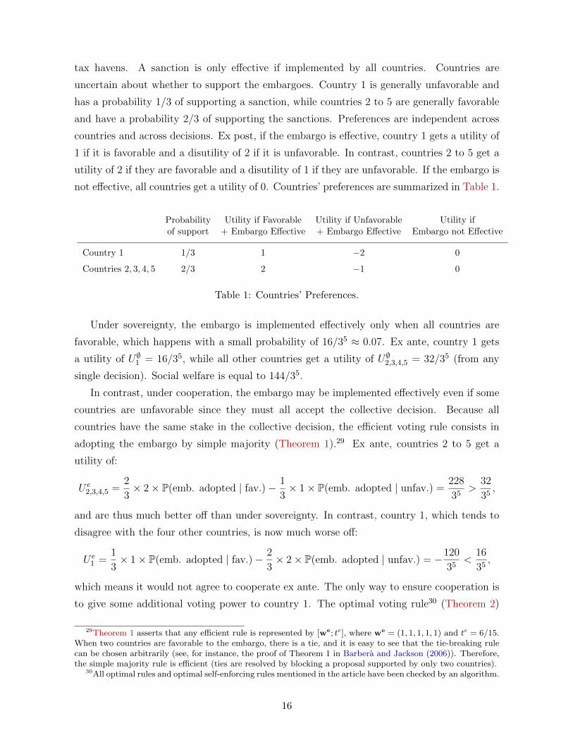
tax havens. A sanction is only effective if implemented by all countries. Countries are
uncertain about whether to support the embargoes. Country 1 is generally unfavorable and
has a probability 1/3 of supporting a sanction, while countries 2 to 5 are generally favorable
and have a probability 2/3 of supporting the sanctions. Preferences are independent across
countries and across decisions. Ex post, if the embargo is effective, country 1 gets a utility of
1 if it is favorable and a disutility of 2 if it is unfavorable. In contrast, countries 2 to 5 get a
utility of 2 if they are favorable and a disutility of 1 if they are unfavorable. If the embargo is
not effective, all countries get a utility of 0. Countries’ preferences are summarized in Table 1.
Probability Utility if Favorable Utility if Unfavorable Utility ifof support + Embargo Effective + Embargo Effective Embargo not Effective
Country 1 1/3 1 −2 0
Countries 2, 3, 4, 5 2/3 2 −1 0
Table 1: Countries’ Preferences.
Under sovereignty, the embargo is implemented effectively only when all countries are
favorable, which happens with a small probability of 16/35 ≈ 0.07. Ex ante, country 1 gets
a utility of U∅1 = 16/35, while all other countries get a utility of U∅2,3,4,5 = 32/35 (from any
single decision). Social welfare is equal to 144/35.
In contrast, under cooperation, the embargo may be implemented effectively even if some
countries are unfavorable since they must all accept the collective decision. Because all
countries have the same stake in the collective decision, the efficient voting rule consists in
adopting the embargo by simple majority (Theorem 1).29 Ex ante, countries 2 to 5 get a
utility of:
U e2,3,4,5 =
2
3× 2× P(emb. adopted | fav.)− 1
3× 1× P(emb. adopted | unfav.) =
228
35>
32
35,
and are thus much better off than under sovereignty. In contrast, country 1, which tends to
disagree with the four other countries, is now much worse off:
U e1 =
1
3× 1× P(emb. adopted | fav.)− 2
3× 2× P(emb. adopted | unfav.) = −120
35<
16
35,
which means it would not agree to cooperate ex ante. The only way to ensure cooperation is
to give some additional voting power to country 1. The optimal voting rule30 (Theorem 2)
29Theorem 1 asserts that any efficient rule is represented by [we; te], where we = (1, 1, 1, 1, 1) and te = 6/15.When two countries are favorable to the embargo, there is a tie, and it is easy to see that the tie-breaking rulecan be chosen arbitrarily (see, for instance, the proof of Theorem 1 in Barbera and Jackson (2006)). Therefore,the simple majority rule is efficient (ties are resolved by blocking a proposal supported by only two countries).
30All optimal rules and optimal self-enforcing rules mentioned in the article have been checked by an algorithm.
16
consists in overweighting country 1 just enough, so that its participation constraint becomes
binding: the embargo is adopted either if country 1 and at least one other country are in
favor or if all but country 1 are in favor. This voting rule can be represented as a weighted
majority rule with weights w∗ = (3, 1, 1, 1, 1) and threshold t∗ = 1/2.31 Country 1 gets
exactly its stand-alone utility, U∗1 = 16/35 = U∅1 , while countries 2 to 5 now get a reduced
utility of U∗2,3,4,5 = 146/35. Social welfare is reduced from 792/35 (under the efficient decision
rule) to 600/35, but still much larger than under sovereignty.
If collective decisions cannot be enforced, countries may choose not to implement the
embargo even if it has been approved collectively. As defined in Section 4, a voting rule is
self-enforcing if there exists a perfect public equilibrium of the associated infinitely repeated
game such that the cooperating profile is played at each stage of the game on the equilibrium
path. In order for a voting rule to be self-enforcing, the benefit of not implementing the
embargo for unfavorable countries must be outweighed by the long-term cost of not sustaining
cooperation, which yields an additional compliance constraint (Proposition 2) that is more
stringent than the original participation constraint. In this example, the optimal voting
rule (with enforcement) cannot be self-enforcing since country 1’s participation constraint
is already binding. Here, self-enforcement can only be achieved by granting veto power to
country 1 (Theorem 3). For δ = 5/6, the optimal self-enforcing rule is such that the embargo
is adopted if and only if country 1 and at least two other countries are in favor. This voting
rule can be represented as a weighted majority rule with weights w∗∗ = (3, 1, 1, 1, 1) and
threshold t∗∗ = 2/3. Country 1 gets a utility of U∗∗1 = 72/35 > U∅1 , while countries 2 to 5 now
get an even more reduced utility of U∗∗2,3,4,5 = 84/35. Social welfare is reduced from 600/35
(under the optimal rule) to 408/35. Note that even though collective decisions cannot be
enforced, social welfare is still much larger under the optimal self-enforcing rule than under
sovereignty. Table 2 summarizes the rules and utilities obtained in each of the four considered
benchmarks (to simplify the expressions, utilities are multiplied by a factor 35).
When the union is divided in two groups of identical countries, the algorithm finds an optimal (resp. optimalself-enforcing) rule among rules that are symmetric within groups. This is without loss of generality, by linearityof the problem. The algorithm is available upon request.
31According to Theorem 2, the optimal rule is represented by [w∗; t∗] with t∗ = 10/21. We note that the ruleis equally well represented by [w∗; 1/2].
17

Benchmark Sovereignty Efficient Optimal Optimal Self-Enforcing
Symbol ∅ e ∗ ∗∗
Voting rule Simple Majority 1 overweighted 1 overweighted + veto
w1 1 3 3
w2,3,4,5 1 1 1
t 1/2 1/2 2/3
U1 ∝ 16 −120 16 72
U2,3,4,5 ∝ 32 228 146 84
Welfare ∝ 144 792 600 408
Table 2: Summary of the example.
6 A Model of Apportionment
In this section, we apply our theory to a model where countries vary along a single dimension:
their population size. At the heart of this more specific model lies a simple process of prefer-
ence formation, where citizens’ preferences are binary and unbiased ex-ante. We assume that
these preferences are correlated within a given country, but independent across countries, and
that each country’s representative follows the national majority. As in Koriyama et al. (2013),
we formalize these assumptions in a parsimonious manner: representatives’ preferences are
first drawn independently across countries, and citizens’ preferences are then derived from
their representative’s preferences by assuming that a fraction q > 1/2 of the country’s pop-
ulation shares the same preference as the representative. Our focus on preferences that are
correlated within countries is akin to the fixed-number of blocks model of Barbera and Jackson
(2006), and is in line with empirical studies on real elections (Gelman et al., 2004). As we
explain below, the main insights of this section would also go through if we assumed that
citizens’ preferences were independent within each country.32
32In that case, it would not be meaningful to start from the preferences of the representatives as in Koriyamaet al. (2013). Instead, we would start from citizens’ preferences, assumed to be independent and identicallydistributed, and define the opinion of the country’s representative as the preference of the majority. This modelcorresponds to the original framework proposed by Penrose (1946), and to the fixed-size block model of Barberaand Jackson (2006). In such a model, the fraction of the population agreeing with the country’s representative,qi, is a random variable. As pi grows large, we obtain qi ≈ 1/2 by the law of large numbers, and qi − 1/2 isapproximately proportional to 1/
√pi, by the central limit theorem.
18

6.1 Model
Under cooperation, proposals are determined exogenously. Ex ante, each country’s represen-
tative has a probability 1/2 of agreeing with any of the proposed reforms, independently of
other countries. In each country, for any given reform, a (randomly chosen) fraction q > 1/2
of citizens agrees with the preference of its country’s representative. If the reform ends up
being implemented effectively (by all countries), favorable citizens get a utility of 1, while
unfavorable citizens get a disutility of 1. If the reform is not adopted effectively, all citizens
get a utility of 0. The probability distribution µ associated with this model is such that:
∀i ∈ N, Pµ (ui = (2q − 1)pi) = Pµ (ui = −(2q − 1)pi) =1
2.
The stake of country i ∈ N is thus given by w+i = w−i = wei /2 = (2q − 1)pi, and its efficient
threshold is tei = 1/2. By normalization, the efficient rule is thus represented by [p; 1/2].33
Under sovereignty, each country now chooses independently which reforms to implement.
In each country, for any given reform, a (randomly chosen) fraction q > 1/2 of citizens agrees
with the reform. Citizens who are favorable get a reduced utility of 1e < 1, while citizens who
are unfavorable get a disutility of 1e . The parameter e > 1 reflects the efficiency gain from
cooperating.34 Ex ante, the aggregate (stand-alone) utility of country i with population pi is
thus equal to:
U∅i = qpi1
e− (1− q)pi
1
e=
(2q − 1)pie
.
In this more specific model of apportionment, countries thus vary in their stakes wei , which
are proportional to their populations pi, but are otherwise identical. Note that Assumption
NEV boils down to pi < (∑
j∈N pj)/2 for all i ∈ N , which means that any country accounts
for less than half of the total population.
6.2 Optimal Voting Rules
We now obtain sharper predictions for the optimal voting rule: first, overweighted countries
are those with the smallest populations; and second, these countries must be given the same
voting weight.
33By contrast, under independent preferences (i.e. qi ≈ 1/2), the stake of country i is w+i = w−i = E[2(qi −
1)pi], which is approximately proportional to√pi, by the central limit theorem. In that case, the efficient rule
is represented by [(√pi)i∈N ; 1/2], this is the original insight of Penrose (1946).
34Note that cooperation is assumed to increase the utility from a favorable reform and the disutility froman unfavorable one, by the same factor e, consistent with the view that the collective action goes further inthe desired/undesired direction. In a previous version of the article, it was assumed that the disutility of anunfavorable reform was multiplied by a factor e−, below or above 1. With that alternative (and more general)assumption, the subsequent Theorem 4 remains valid, with a suitable adaptation of the threshold of the optimalrule.
19

Theorem 4. In the model of apportionment, there exists p ∈ R such that any optimal voting
rule is a weighted majority rule represented by [w∗; 1/2], with w∗i = max(pi, p) for all i ∈ N .
The intuition behind the result of Theorem 4 is as follows. Start from the efficient weights,
which are here proportional to the populations. Smaller countries have a smaller weight and
therefore enjoy a smaller probability of success : their probability of agreeing with the collective
decision is lower. In turn their utilities are lower, relative to their stand-alone utilities. If
the efficient rule does not satisfy the participation constraints, then it can be adjusted by
increasing the weights of smaller countries, up to the level at which their constraints bind.35
Figure 2: Optimal weights (absolute and per capita) in the model of apportionment
population pi
optimal weight w∗i
p
w∗i = piw∗i = p
population pi
w∗i /pi
p
The optimal apportionment rule is illustrated in Figure 3, in absolute and per-capita terms.
We first note that the distribution of weights is degressively proportional : weights increase
with countries’ populations (left panel’s curve is increasing), but less than proportionally
(right panel’s curve is decreasing). A sizeable literature on apportionment has already argued
in favor of this property,36 but on different grounds than the one we put forth here. In
particular, our argument focuses on the bottom of the distribution and supports overweighting
small countries that may otherwise have almost no say in the collective decisions. By contrast,
previous models recommend degressively proportional rules that have noticeable implications
for medium to larger states, often with weights in the order of pα with 1/2 ≤ α ≤ 1.37
The requirement that smaller countries shall be given a minimal and equal representation
is actually found explicitly in the Treaty of Lisbon, which specifies a set of constraints for the
35The argument similarly applies in the case of independent preferences (i.e. qi ≈ 1/2). In that case,the optimal weights are equal to: w∗i = max(
√pi, w). The main insights thus remain: smaller countries are
overweighted, and they receive the same weight.36Laslier (2012) offers a review of the different arguments in favor of such rules.37For instance, in the model of Barbera and Jackson (2006), the optimal α is approximately equal to 1/2
in the fixed-size block model, and equal to 1 in the fixed-number-of-blocks model. See also Beisbart and Bovens(2007).
20

composition of the European Parliament.38 Indeed, article 14.2 states that “representation
of citizens [in the European Parliament] shall be degressively proportional, with a minimum
threshold of six members per Member State” (Treaty of Lisbon, 2007a). Our article thus
offers a theoretical rationale for such a minimal representation threshold.
Finally, the apportionment formula proposed here combines in a simple manner the no-
tions of proportionality and equality, which is reminiscent of several prominent examples.
In particular, the overweighting of smaller states echoes the distribution of seats in the U.S.
Electoral College,39 and the optimal weights per capita observed in the right panel of Figure 3
mirror the actual ones exhibited in Figure 1. The eight smaller states are allocated the same
number of three seats,40 representing 4.5% of the seats for only 1.9% of the total population.
The same type of apportionment formula has also been proposed for the allocation of seats
in the European Parliament, under the name of Cambridge Compromise.41
6.3 Heterogeneous Gains
Our basic model of apportionment assumes that citizens in all countries benefit from the
same level of efficiency gain from cooperation. However, it might be sensible in some appli-
cations to assume that efficiency gains decrease with a country’s population, larger countries
being usually less dependent on international cooperation than smaller countries. In order to
investigate the implications of this more general assumption, we introduce a model of appor-
tionment with heterogeneous gains, where each country is characterized by a possibly different
efficiency gain ei ∈ (1,+∞).
In this more complex model, the efficient rule remains the same (the weighted rule [p; 1/2])
and the stand-alone utilities become U∅i =(2q − 1)pi
ei. The reasoning conducted in the proof
of Theorem 4 does not extend directly, but we obtain a similar characterization of the optinal
weights by resorting to an approximation. The difficulty lies in precisely estimating the
expected utility Ui(v), which is proportional to the product of country i’s population pi to
its Banzhaf voting power under rule v, that we denote BZi(v).42 We use the Penrose limit
approximation (Lindner and Machover, 2004), stating that for n large enough, the ratio of
any two countries’ voting power under a weighted voting rule represented by [w; 1/2] can be
38For a discussion of the application to the allocation of seats in a federal parliament, rather than votingweights in a federal council, see Koriyama et al. (2013).
39Each state is allocated a baseline of two electors plus a number of electors proportional to its population.40Alaska, Delaware, District of Columbia, Montana, North Dakota, South Dakota, Vermont, and Wyoming.41The Cambridge Compromise was the result of an academic initiative by the European Parliament, which
aimed at formulating a transparent and fair allocation of the seats in the European Parliament. The proposedallocation is based on a similar base + prop formula as in the U.S. Electoral College, whereby each country isallocated a base of six seats plus a number of seats proportional to its population. See Grimmett (2012).
42The Banzhaf index (Banzhaf, 1964) is a standard measure of ex ante voting power in committees, given by
the following formula: BZi(v) =1
2n−1
∑S⊆N,i∈S [v(S)− v(S\{i})] .
21
approximated by the ratio of their respective voting weights.43
Proposition 3. In the model of apportionment with heterogeneous gains, under the Penrose
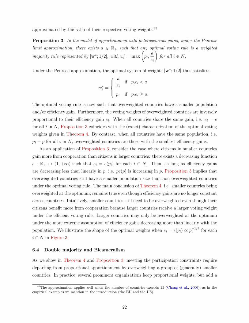
limit approximation, there exists a ∈ R+ such that any optimal voting rule is a weighted
majority rule represented by [w∗; 1/2], with w∗i = max
(pi,
a
ei
)for all i ∈ N .
Under the Penrose approximation, the optimal system of weights [w∗; 1/2] thus satisfies:
w∗i =
a
eiif piei < a
pi if piei ≥ a.
The optimal voting rule is now such that overweighted countries have a smaller population
and/or efficiency gain. Furthermore, the voting weights of overweighted countries are inversely
proportional to their efficiency gain ei. When all countries share the same gain, i.e. ei = e
for all i in N , Proposition 3 coincides with the (exact) characterization of the optimal voting
weights given in Theorem 4. By contrast, when all countries have the same population, i.e.
pi = p for all i in N , overweighted countries are those with the smallest efficiency gains.
As an application of Proposition 3, consider the case where citizens in smaller countries
gain more from cooperation than citizens in larger countries: there exists a decreasing function
e : R+ 7→ (1,+∞) such that ei = e(pi) for each i ∈ N . Then, as long as efficiency gains
are decreasing less than linearly in p, i.e. pe(p) is increasing in p, Proposition 3 implies that
overweighted countries still have a smaller population size than non overweighted countries
under the optimal voting rule. The main conclusion of Theorem 4, i.e. smaller countries being
overweighted at the optimum, remains true even though efficiency gains are no longer constant
across countries. Intuitively, smaller countries still need to be overweighted even though their
citizens benefit more from cooperation because larger countries receive a larger voting weight
under the efficient voting rule. Larger countries may only be overweighted at the optimum
under the more extreme assumption of efficiency gains decreasing more than linearly with the
population. We illustrate the shape of the optimal weights when ei = e(pi) ∝ p−1/4i for each
i ∈ N in Figure 3.
6.4 Double majority and Bicameralism
As we show in Theorem 4 and Proposition 3, meeting the participation constraints require
departing from proportional apportionment by overweighting a group of (generally) smaller
countries. In practice, several prominent organizations keep proportional weights, but add a
43The approximation applies well when the number of countries exceeds 15 (Chang et al., 2006), as in theempirical examples we mention in the introduction (the EU and the US).
22

Figure 3: Optimal weights (absolute and per capita) in the model of apportionment with
heterogeneous gains for ei ∝ p−1/4i
population pi
optimal weight w∗i
p
w∗i = pi
w∗i = a/ei
population pi
w∗i /pi
p
requirement on the number of favorable countries for a proposal to be accepted. This is the
case for example at the Council of the European Union, where a proposal needs the support
of at least 55% of countries, representing at least 65% of the total population of the EU.
The US bicameral legislative system, although of a different nature, can also be interpreted
as a form of double majority if one assumes that representatives from the same state vote
identically. A successful proposal then requires the support of at least 26 states (through the
Senate), representing at least 50% of the population (through the House of Representatives).
Formally, a rule v is an efficient rule with size threshold if there exist an efficient rule ve
and a size threshold k ∈ {0, . . . , n} such that, for any profile of votes m = (mi)i∈N ∈ {0, 1}N ,{#{i | mi = 1} ≥ k ⇒ v(m) = ve(m)
#{i | mi = 1} < k ⇒ v(m) = 0.
We write v = ve ⊕ k. Note that such a rule v is not a weighted rule in general, and thus
cannot be optimal.44 As we show in the following proposition, even though these rules are
not optimal, they are more likely to satisfy the participation constraints than the efficient
voting rule itself.
Proposition 4. In the apportionment model, assuming that no two countries have the same
population and that one country is more populated than a group of two other countries, there
44Whenever the vector of populations is far from being collinear to the constant vector, one may apply thecharacterization of weighted voting in Taylor and Zwicker (1992) to show that an efficient rule with (positive)size threshold is not weighted. For instance, if p = (1, 10, 10, 10, 10, 100, 100), the rule v = ve⊕ 4 is not weightedas v(1236) = v(1457) = 1 but v(12345) = v(167) = 0, violating the property of trade robustness. A similarargument implies that the rule of the Council of the EU is not weighted.
23

exist two thresholds e, e ∈ (1,+∞), with e < e, such that:
(i) if e ≥ e, then the efficient voting rule satisfies the participation constraints.
(ii) if e ≤ e < e, then the efficient voting rule does not satisfy the participation constraints
but there exists k∗ > 0 such that the efficient rule with size threshold k∗ does.
(iii) if e < e, then none of the efficient rules with size threshold satisfy the participation
constraints.
The main message of Proposition 4 is contained in statement (ii): for intermediate ef-
ficiency gains, adding a certain size threshold k∗ to the efficient rule allows to satisfy the
participation constraints. Note that the assumption under which the statement holds is very
mild: it simply requires that countries’ populations are not too similar from each other.45
To illustrate the effect of the size threshold on states’ ability to satisfy their participation
constraints, we plot in Figure 4 the voting power of a U.S. state’s representative as a function
of the state’s population. Note that the voting power is here proportional to Ui(v)/U∅i ,
the ratio that determines whether a state satisfies its participation constraint. We plot the
corresponding graphs for several rules: the efficient rule ve represented by [p; 1/2], and the
efficient rules with size threshold k, ve ⊕ k, for k ∈ {24, 26, 28, 30}.
Figure 4: Voting power of a state’s representative, as a function of the state’s population, forefficient rules with varying size thresholds, for the U.S. (2017 population figures)
●●●●●●●●●●●●●●●●
●●●●●●●●●●
●●●●●●●●
●●●●●●
●●●●
●●●
●●
●
●
0.00
0.05
0.10
0.15
0.20
0.25
0 10 20 30 40
State population (millions)
Vot
ing
Pow
er
Size threshold k
● 0
24
26
28
30
We observe in Figure 4 the two effects associated with the introduction of a size threshold.
45For instance, it is satisfied in the EU as Germany is more populated than Malta and Luxembourg takentogether, and in the U.S. as California is more populated than Alabama and Arkansas taken together.
24

Starting from the efficient voting rule (k = 0), introducing a small size threshold induces first
a distributional effect: smaller countries gain with respect to the efficient benchmark while
larger countries lose.46 This effect is at the heart of Proposition 4 because increasing the
utility of the smallest country makes all countries more likely to satisfy the participation
constraints. As the size threshold increases, a second effect comes into play: the rule becomes
more stringent, making proposals more difficult to pass, which may ultimately decrease the
utility of all countries. This is for example the case in the U.S. legislature when the size
threshold goes from 26 to 30.
We conclude that, while not as efficient as the optimal voting rules, double majority rules
similarly depart from efficiency by accommodating smaller countries.47
6.5 Optimal Self-Enforcing Rules
Finally, we investigate the shape of optimal self-enforcing rules in the model of apportionment.
We also obtain sharper predictions: either no country has veto power or all countries have
it, and we can map these two cases on a graph parametrized by the efficiency gain e and the
discount factor δ.
Theorem 5. In the model of apportionment, any optimal self-enforcing rule is either the
unanimity rule or a weighted majority rule for which no country has veto power. There exist
a threshold e > 1, and two non-increasing functions δc, δeff : (1,+∞) → R+, such that
δc(e) ≤ δeff (e) for all e > 1, lime→∞ δeff (e) < 1, and:
(i) if δ ≥ δeff (e), any optimal self-enforcing rule is an efficient weighted majority rule,
(ii) if δc(e) ≤ δ < δeff (e), any optimal self-enforcing rule is a weighted majority rule, with
overweighting of small countries,
(iii) if δ < δc(e) and e ≥ e, the optimal self-enforcing rule is the unanimity rule,
(iv) if δ < δc(e) and e < e, there is no self-enforcing rule.
Moreover, for δc(e) ≤ δ < δeff (e), there exists a minimal weight p(e, δ), non-increasing in
both e and δ, such that any optimal self-enforcing rule is represented by [w∗∗; 1/2], defined by
w∗∗i = max(pi, p(e, δ)
)for all i ∈ N .
Theorem 5 defines four regions in the space (e, δ) that yield different (or no) optimal self-
enforcing rules, as represented in Figure 5 below.
46Formally, we can show that the difference in utility associated to the introduction of the size threshold,relative to the stand-alone utility, is decreasing with a country’s population.
47One may wonder what is the loss of welfare associated to an efficient rule with size threshold, compared tothe optimal rule. As an exercise, we computed for each size threshold k > 10 the minimal level of efficiency gaine for which ve ⊕ k satisfies the participation constraints and the optimal rule associated to e. Numerically, weobserve that the optimal rule always fills at least 66.8% of the welfare gap between ve ⊕ k and the efficient ruleve.
25

Figure 5: Optimal self-enforcing rule in the model of apportionment
e
1Weighted majority (efficient)
Weighted majority (overweighting)
UnanimityNo cooperation
efficiency gain e0
discount factor δ
δc(e)
δeff (e)
The figure can be interpreted either horizontally or vertically. First, the line δ = 1 depicts
the results we obtain for enforceable decisions. If the efficiency gain e is too small, there
is no rule inducing cooperation. If the efficiency gain e is large enough, the efficient voting
rule induces cooperation and is therefore optimal. However, for intermediate values of e, the
optimal rule involves overweighting small countries, and the extent to which small countries
are overweighted decreases with e.
Reading Figure 5 vertically reveals how Theorem 5 extends the main result of Maggi and
Morelli (2006). In that article, countries are homogeneous, and there exists a threshold δ,
below which the optimal self-enforcing rule is the unanimity, and above which the optimal
self-enforcing rule is the (efficient) majority rule. In our model, for e ≥ e, there are two
thresholds: δeff (e) and δc(e). As in the homogeneous model, the optimal self-enforcing rule
is the efficient rule when the discount factor is high (δ ≥ δeff (e)), and it is the unanimity
rule when the discount factor is low (δ < δc(e)). What is new here is that we obtain a region
of intermediate values of the discount factor (δc(e) ≤ δ < δeff (e)), for which the optimal self-
enforcing rule is an inefficient weighted majority rule, with overweighting of small countries.
Moreover, the extent to which small countries are overweighted decreases with the efficiency
gain e and with the discount factor δ.
7 Conclusion
We have studied the design of voting rules in representative committees when decisions are bi-
nary and cooperation is voluntary. In contrast to the efficient voting rule, which assigns to each
26

country a voting weight proportional to its stake, the optimal voting rule sometimes involves
overweighting certain countries, namely those that have the lowest endogenous incentive to
cooperate. In the apportionment case, where the heterogeneity reduces to the population
size and countries have identical ex-ante preferences, the optimal voting rule assigns an equal
(and larger than proportional) weight to smaller countries, while larger countries keep their
efficient weight. The theory thus provides a new rationale for the use of degressive propor-
tional apportionment rules. When collective decisions are not enforceable, and cooperation
must be agreed on repeatedly, voting rules must satisfy stronger compliance constraints, thus
reducing social welfare. At the optimum, countries that do not satisfy compliance constraints
benefit from veto power. In the apportionment case, the optimal self-enforcing rule is either
unanimous (thus giving veto power to all countries), or such that no country enjoys veto
power.
We have assumed throughout the article that cooperation was only beneficial if all coun-
tries participated, the “pure” collective action case (Maggi and Morelli, 2006).48 Note that
all of our results on enforceable decisions remain valid for more general forms of cooperation
gains. Indeed, as participation is decided at the unanimity in our model, either all countries
cooperate or all remain sovereign. Nevertheless, inducing the cooperation of all countries may
prove costly, as in our main example, in which the welfare drops by 24% from the efficient
to the optimal rule. When the cooperation gains are “impure”, this cost may be alleviated
by allowing a strict subset of countries to cooperate while the others remain sovereign.49 Ex-
tending the model to such flexible forms of cooperation seems a promising avenue for further
research.
We have taken a “constrained” normative approach where a benevolent social planner
looks for the welfare-maximizing voting rule while accounting for the effect of the rule on
countries’ participation and compliance. A natural alternative would be to consider a fully
positive approach where countries bargain over the voting rule. The first participation stage
in our game (as described in Section 2) could then be replaced by a bargaining stage where
the voting rule (to be used in the subsequent stages) is determined by the following Nash
program:
maxv∈V
∏i∈N
(Ui(v)− U∅i
).
48The “pure” collective action case applies whenever the failure to cooperate of even one country can jeopardizethe success of the considered policy. Examples include climate change agreements, immigration policy, oragreements not to harbor terrorists.
49This flexible form of cooperation, known as enhanced cooperation, was first introduced by the EuropeanUnion in the Treaty of Amsterdam (1997). It allows a subset of nine or more countries to move forward withcooperation without the consent of the other countries.
27

The rest of the game would follow in the same fashion. In contrast to the original model,
the voting rule is not chosen exogenously so as to maximize social welfare but is obtained
endogenously as the outcome of a Nash bargaining between countries in the initial stage. As
we explain in Section A.9 in the Appendix, one can show that under enforceable decisions
the outcome is a weighted voting rule such that countries that are closer to their stand-alone
utility under the bargained voting rule are relatively more overweighted. The result captures
a similar intuition as Theorem 2. Countries that gain less from cooperation (relative to their
outside option) under the bargained voting rule are more overweighted. For instance, in the
example of Section 5, the bargained rule can be represented as a weighted majority rule with
weights (4, 1, 1, 1, 1) and a threshold of 1/2.50 Country 1’s utility increases from 16/35 (under
the optimal voting rule) to 38.8/35, while the utility of countries 2 to 5 decreases from 146/35
to 123.2/35. Social welfare decreases from 600/35 to 531.6/35. More generally, overweighted
countries under the optimal voting rule are necessarily better off under the bargained vot-
ing rule since their utility under the optimal voting rule is equal to their stand-alone utility.
However, social welfare is necessarily lower since the bargained voting rule satisfies all partic-
ipation constraints. Finally, note that the bargained voting rule is more difficult to compute
algebraically because it is defined as the solution of a non-linear maximization problem.
References
Alesina, A., Angeloni, I., and Etro, F. (2005). International unions. American Economic
Review, 95(3):602–615.
Alesina, A. and Spolaore, E. (1997). On the number and size of nations. The Quarterly
Journal of Economics, 112(4):1027–1056.
Athey, S. and Bagwell, K. (2001). Optimal collusion with private information. RAND Journal
of Economics, pages 428–465.
Azrieli, Y. and Kim, S. (2014). Pareto efficiency and weighted majority rules. International
Economic Review, 55(4):1067–1088.
Balinski, M. L. and Young, H. P. (1982). Fair representation: Meeting the ideal of one man,
one vote. Yale University Press.
Banzhaf, J. F. (1964). Weighted voting doesn’t work: A mathematical analysis. Rutgers L.
Rev., 19:317.
50And such that the embargo is approved with probability 0.65 if all but country 1 are in favor and withprobability 0.4 if only country 1 is in favor.
28

Barbera, S. and Jackson, M. O. (2004). Choosing how to choose: Self-stable majority rules
and constitutions. The Quarterly Journal of Economics, 119(3):1011–1048.
Barbera, S. and Jackson, M. O. (2006). On the weights of nations: Assigning voting power
to heterogeneous voters. Journal of Political Economy, 114(2):317–339.
Beisbart, C. and Bovens, L. (2007). Welfarist evaluations of decision rules for boards of
representatives. Social Choice and Welfare, 29(4):581–608.
Bouton, L., Llorente-Saguer, A., and Malherbe, F. (2018). Get rid of unanimity rule: The
superiority of majority rules with veto power. Journal of Political Economy, 126(1):107–
149.
Bown, C. (2004). On the economic success of gatt/wto dispute settlement. The Review of
Economics and Statistics, 86:811–823.
Brighouse, H. and Fleurbaey, M. (2010). Democracy and proportionality. Journal of Political
Philosophy, 18(2):137–155.
Casella, A. (1992). Participation in a currency union. American Economic Review, 82(4):847–
63.
Chang, P.-L., Chua, V. C., and Machover, M. (2006). Ls penrose’s limit theorem: tests by
simulation. Mathematical Social Sciences, 51(1):90–106.
Cremer, J. and Palfrey, T. R. (1996). In or out? centralization by majority vote. European
Economic Review, 40(1):43–60.
Demange, G. (2017). The stability of group formation. Revue d’economie politique,
127(4):495–516.
Felsenthal, D. S. and Machover, M. (1999). Minimizing the mean majority deficit: The second
square-root rule. Mathematical Social Sciences, 37(1):25–37.
Gelman, A., Katz, J. N., and Bafumi, J. (2004). Standard voting power indexes do not work:
an empirical analysis. British Journal of Political Science, 34(04):657–674.
Grimmett, G. R. (2012). European apportionment via the cambridge compromise. Mathe-
matical Social Sciences, 63(2):68–73.
Koriyama, Y., Laslier, J.-F., Mace, A., and Treibich, R. (2013). Optimal apportionment.
Journal of Political Economy, 121(3):584–608.
29

Kurz, S., Maaser, N., and Napel, S. (2017). On the democratic weights of nations. Journal
of Political Economy, 125(5):1599–1634.
Laslier, J.-F. (2012). Why not proportional? Mathematical Social Sciences, 63(2):90–93.
Lindner, I. and Machover, M. (2004). Ls penrose’s limit theorem: proof of some special cases.
Mathematical Social Sciences, 47(1):37–49.
Loeper, A. (2011). Coordination in heterogeneous federal systems. Journal of Public Eco-
nomics, 95(7):900–912.
Maggi, G. and Morelli, M. (2006). Self-enforcing voting in international organizations. The
American Economic Review, 96(4):1137–1158.
Moravcsik, A. (1998). The choice for Europe: social purpose and state power from Messina
to Maastricht. Cornell University Press.
Penn, E. M. (2016). Engagement, disengagement, or exit: A theory of equilibrium associa-
tions. American Journal of Political Science, 60(2):322–336.
Penrose, L. S. (1946). The elementary statistics of majority voting. Journal of the Royal
Statistical Society, 109(1):53–57.
Rae, D. W. (1969). Decision-rules and individual values in constitutional choice. American
Political Science Review, 63(1):40–56.
Renou, L. (2011). Group formation and governance. Journal of Public Economic Theory,
13(4):595–630.
Taylor, A. and Zwicker, W. (1992). A characterization of weighted voting. Proceedings of the
American Mathematical Society, 115(4):1089–1094.
Treaty of Lisbon (2007a). Consolidated version of the treaty on european union - title i:
Common provisions.
Treaty of Lisbon (2007b). Consolidated version of the treaty on the functioning of the euro-
pean union - part one: Principles.
Wilcox, F. O. (1945). The yalta voting formula. American Political Science Review, 39(5):943–
956.
30

A Appendix: Proofs
A.1 Proof of Proposition 1
In the game ΓE(v), the only relevant beliefs are given by the prior µ at the first stage, and
by µ(ui, ·) for a player i at the third stage. Thus, the only condition to check to see if the
cooperating profile is a perfect Bayesian equilibrium is that of sequential rationality.
First, it is clear that sending mi = 1ui>0 is always rational in the third stage, as v is
non-decreasing. Second, playing di = 1 at the first stage is rational if and only if the expected
outcome of the game under cooperation is no worse than under sovereignty (obtained if
di = 0). The result follows.
A.2 Proof of Theorem 2
In this proof, and in the subsequent proofs, we abuse notation and write v(M) for v(m),
where M ⊆ N denotes the coalition of countries that vote in favor of the proposal: M = {i ∈N |mi = 1}.
Let V∗ = arg maxv∈V1 W (v) be the set of optimal rules. The set V∗ is convex: for any
v, v′ ∈ V∗ and α ∈ (0, 1), it is clear that αv + (1 − α)v′ ∈ V∗, by linearity of the objective
function and of the constraints that define V∗. Let v∗ be an optimal rule such that:
v∗ ∈ arg max #{M ⊆ N |v(M) ∈ (0, 1)}.
In words, the rule v∗ maximizes the recourse to probabilistic tie-breaking among optimal
rules. We claim that, if v∗ is represented by [w; t], then any optimal rule v′ ∈ V∗ is also
represented by [w; t]. To see that, assume that v∗ is represented by [w; t], but that v′ ∈ V∗
is not. Then, without loss of generality, we can assume that there exists M ⊆ N , such that∑i∈M wi > t
∑i∈N wi, but v′(M) < 1. We have by assumption v∗(M) = 1. We obtain a
contradiction by considering the rule v′′ = (v∗ + v′)/2, as v′′ ∈ V∗, but #{M ⊆ N |v′′(M) ∈(0, 1)} > #{M ⊆ N |v∗(M) ∈ (0, 1)}. In the remainder of the proof, we solely focus on v∗, as
we know that any representation of v∗ will be a representation of any optimal rule.
We claim that v∗ is also a solution of the following maximization problem (note that v is
not constrained to be non-decreasing in that problem) :
(P) :
∣∣∣∣∣∣∣max
{v(M)}M⊆N∈[0,1](2N )
∑i∈N
Ui(v)
s.t. ∀i ∈ N, Ui(v) ≥ U∅i .
It suffices to show that any solution of (P) is non-decreasing. For that, let v be a solution of
(P) such that v(M) > v(M ′) with M ⊂ M ′. It is straightforward that the rule v′, obtained
from v by permuting M and M ′, will increase the expected utility of countries in M ′\M , while
31

decreasing the expected utility of no country. Hence, v′ improves the welfare and satisfies the
constraints, a contradiction.
Let P be the probability distribution on the coalitions M of countries favoring the reform
(under truthful voting), induced by the probability distribution µ. Formally:
∀M ⊆ N, P (M) = Pµ ({i|ui > 0} = M) .
By assumption, we have that for all M ⊆ N , P (M) > 0. As countries’ utilities are indepen-
dent, the expected utility of a country i ∈ N under a rule v writes
Ui(v) = Eµ[v((1uj>0)j∈N )ui
]=∑
M,i∈MP (M)v(M)Eµ [ui|ui > 0] +
∑M,i/∈M
P (M)v(M)Eµ [ui|ui < 0]
=∑
M,i∈MP (M)v(M)w+
i −∑
M,i/∈M
P (M)v(M)w−i .
The Lagrangian of the problem (P) writes
L(v) =∑i∈N
Ui(v) +∑i∈N
λi[Ui(v)− U∅i ] +∑M⊆N
[ηMv(M) + νM (1− v(M))].
Its partial derivative with respect to v(M) (one of the 2n variables) is
∂L∂v(M)
(v) = P (M)
(∑i∈M
(1 + λi)w+i −
∑i/∈M
(1 + λi)w−i
)+ ηM − νM .
As v∗ is a solution of (P), we can apply the first-order conditions of the Kuhn-Tucker theorem
(the constraints are affine functions). There exist non-negative coefficients (λi, ηM , νM )i∈N,M⊆N
such that
(i) ∀M ⊆ N,∂L
∂v(M)(v∗) = 0
(ii) ∀i ∈ N, λi[Ui(v∗)− U∅i ] = 0
(iii) ∀M ⊆ N, ηMv∗(M) = 0
(iv) ∀M ⊆ N, νM (1− v∗(M)) = 0.
By the last two lines, ηM and νM cannot be simultaneously positive. Therefore, we have{ηM − νM < 0 ⇒ νM > 0 ⇒ v∗(M) = 1
ηM − νM > 0 ⇒ ηM > 0 ⇒ v∗(M) = 0.
32

By (i), and the formula for the derivative of the Lagrangian, we have that
ηM − νM < 0 ⇔∑i∈M
(1 + λi)w+i >
∑i/∈M
(1 + λi)w−i
⇔∑i∈M
(1 + λi)(w+i + w−i ) >
∑i∈N
(1 + λi)w−i
⇔∑i∈M
(1 + λi)wei >
∑i∈N
(1 + λi)w−i∑i∈N
(1 + λi)wei
∑i∈N
(1 + λi)wei .
Setting w∗i = (1 + λi)wei and
t∗ =
∑i∈N
(1 + λi)w−i∑i∈N
(1 + λi)wei=
∑i∈N
w∗i tei∑
i∈Nw∗i
,
we get that:
∀M ⊆ N,
∑i∈M
w∗i > t∗∑i∈N
w∗i ⇒ v∗(M) = 1∑i∈M
w∗i < t∗∑i∈N
w∗i ⇒ v∗(M) = 0.
Therefore we conclude that v∗, and thus any optimal rule in V∗, is weighted and can be
represented by [w∗; t∗]. Moreover, by application of the Kuhn-Tucker conditions, we have
that Ui(v∗) = U∅i ⇒ λi ≥ 0⇒ w∗i ≥ wei and Ui(v
∗) > U∅i ⇒ λi = 0⇒ w∗i = wei .
A.3 Proof of Proposition 2
The proof is divided in two steps. First, we construct a profile of the repeated game, with
cooperation at each stage on the equilibrium path, and we show that it is a perfect public
equilibrium if the constraints of the proposition are satisfied. Second, we show that if one
constraint is not satisfied, no perfect public equilibrium can sustain cooperation on the equi-
librium path.
Step 1: Let v be a voting rule that satisfies the constraints of Proposition 2. We consider
the following profile of strategies:
• At each stage T , play the cooperative profile of the game ΓNE(v).
• If exactly one country is observed to deviate at time T (either dTi = 0 or aTi 6= vT (mT )
for some i ∈ N), then all countries choose to remain sovereign in any subsequent stage
T ′ > T .
33
Consider a potential deviation from the previous profile, for some country i, and assume it is
a (strict) best reply. We note (d0i ,m0i , a
0i ) the first stage of this deviation.
If d0i = 0, the deviation yields a stage payoff U∅i , and a future payoff U∅i (given the trigger
strategies employed by other players). As Ui(v) ≥ U∅i (each country satisfies at least the
participation constraint), this deviation is not profitable.
If d0i = 1, and the deviation is such that ∃ui ∈ R,m0i (ui) 6= 1ui>0, then it is (weakly)
dominated by the strategy (d0i ,1ui>0, a0i ). Indeed, as the rule v is non-decreasing, lying only
makes it more likely for the action plan v(m) to go against the country’s will, which is never
beneficial, and it doesn’t changes what happens at subsequent stages at it cannot be detected.
We may thus assume that m0i = 1ui>0.
Let ui ∈ R and m−i ∈ {0, 1}N\{i} be such that µ(ui) > 0 and a0i 6= v(1ui>0,m−i). As the
deviation will be detected, it must yield a stage-payoff of more than
v(1ui>0,m−i)ui +δ
1− δ(Ui(v)− U∅i )
(because of the trigger strategies). This deviation can only be profitable if ui < 0. We then
distinguish two cases:
• If i has veto power, since 1ui>0 = 0, we have v(1ui>0,m−i) = 0. Therefore, the deviation
is not profitable.
• If i has no veto, we have:
v(1ui>0,m−i)ui +δ
1− δ(Ui(v)− U∅i ) ≥ −wDi +
δ
1− δ(Ui(v)− U∅i ) ≥ 0
because i satisfies the compliance constraint. Therefore, the deviation is not profitable.
Finally, we conclude that the proposed profile of strategies is a perfect public equilibrium.
Step 2: Now suppose that there exists i ∈ V E(v) such that Ui(v) < U∅i . Consider a profile
such that cooperation is chosen at any stage, and (vT (1uTi >0)i∈N ) is always implemented.
Country i’s expected utility is Ui(v). Therefore, playing dTi = 0 for all T is a profitable
deviation.
Alternatively, suppose that there exists i /∈ V E(v) such that Ui(v) < U∅i +1− δδ
wDi .
Consider a profile such that cooperation is chosen at any stage, and (vT (1uTi >0)i∈N ) is always
implemented. Consider the following deviation of player i: follow the first profile, and if there
exists some T such that ui = −wDi , then play aTi = 0, and dT′
i = 0 for all T ′ > T . The event
{uTi = −wDi } occurs almost surely in finite time (for T < +∞), and yields a superior payoff
when it occurs. This is thus a profitable deviation.
34

A.4 Proof of Theorem 3
Let v∗∗ be an optimal self-enforcing rule, and let V ∗∗ = V E(v∗∗) be its set of veto coun-
tries. By definition, v∗∗ is solution of the problem maxv∈Vδ W (v), which is equivalent to
maxV⊆N maxv∈Vδ,V E(v)=V W (v). Therefore, v∗∗ is solution of maxv∈Vδ,V E(v)=V ∗∗W (v), and
by the argument made at the beginning of the proof of Theorem 2, the rule v∗∗ is also a
solution of:
(PV ∗∗) :
∣∣∣∣∣∣∣∣∣∣∣
max{v(M)}V ∗∗⊆M⊆N∑
i∈N Ui(v)
s.t. ∀i ∈ V ∗∗, Ui(v) ≥ U∅i
s.t. ∀i ∈ N\V ∗∗, Ui(v) ≥ U∅i +1− δδ
wDi
s.t. ∀M, V ∗∗ *M ⇒ v(M) = 0.
Now, by the arguments made in the proof of Theorem 2, if λi denotes the Lagrange multiplier
associated to country i’s constraint in (PV ∗∗), and if we note w0i = (1 + λi)wei and
t0 =
∑i∈N
w0i tei∑
i∈Nw0i
,
we obtain:
∀M ⊆ N, V ∗∗ ⊆M,
∑i∈M
w0i > t0
∑i∈N
w0i ⇒ v∗∗(M) = 1∑
i∈Mw0i < t0
∑i∈N
w0i ⇒ v∗∗(M) = 0.
Moreover, we know that V ∗∗ * M ⇒ v∗∗(M) = 0. Now, we define w∗∗i = w0i + K1i∈V ∗∗ ,
where K is defined as a sufficiently large number, for instance K = 1 +∑
i∈N w0i . We obtain
that if∑
i∈M w∗∗i > t0∑
i∈N w0i + K#V ∗∗, then V ∗∗ ⊆ M and
∑i∈M w0
i > t0∑
i∈N w0i , and
therefore v∗∗(M) = 1. We also have that if∑
i∈M w∗∗i < t0∑
i∈N w0i +K#V ∗∗, then V ∗∗ *M
or∑
i∈M w0i < t0
∑i∈N w
0i , and therefore v∗∗(M) = 0. Finally, denoting
t∗∗ =1∑
i∈Nw∗∗i
(t0∑i∈N
w0i +K#V ∗∗
)
We obtain that:
∀M ⊆ N,
∑i∈M
w∗∗i > t∗∗∑i∈N
w∗∗i ⇒ v∗∗(M) = 1∑i∈M
w∗∗i < t∗∗∑i∈N
w∗∗i ⇒ v∗∗(M) = 0.
35

This means that v∗∗ is represented by [w∗∗; t∗∗]. Furthermore, note that:
t∗∗ =1∑
i∈Nw∗∗i
(∑i∈N
w0i tei +K#V ∗∗
)
=1∑
i∈Nw∗∗i
(∑i∈N
witei +K
∑i∈V ∗∗
(1− tei )
)≥
∑i∈N
w∗∗i tei∑
i∈Nw∗∗i
.
Finally, let i ∈ N be a country such that Ui(v∗∗) < U∅i +
1− δδ
wDi . As we have assumed
that v∗∗ is self-enforcing, it must be that i ∈ V E(v∗∗). Then, by construction, we obtain that
w∗∗i > w0i ≥ wei .
Conversely, let i ∈ N be a country such that Ui(v∗∗) > U∅i +
1− δδ
wDi . We then show
that i has no veto power under v∗∗. By contradiction, suppose that i has veto power. Then,
v∗∗(N\{i}) = 0. For ε > 0, consider vε defined by:{vε(N\{i}) = ε
∀M 6= N\{i}, vε(M) = v∗∗(M).
We have Ui(vε) = Ui(v
∗∗)−εP (N\{i})w−i and ∀j 6= i, Uj(vε) = Uj(v
∗∗)+εP (N\{i})w+j . By
Assumption NEV, we get W (vε) > W (v∗∗). Moreover, vε is self-enforcing for ε small enough,
hence a contradiction. We obtain that i /∈ V E(v∗∗). It follows that w∗∗i = w0i = wei .
A.5 Proof of Theorem 4
We now have:
Ui(v) =(2q − 1)pi
2n
∑M, i∈M
v(M)−∑
M, i/∈M
v(M)
.
and U∅i = (2q − 1)pi/e. Let v∗ be an optimal rule maximizing the recourse to probabilistic
tie-breaking (i.e. chosen as in the proof of Theorem 2, as we know that any representation
of v∗ will be a representation of any optimal rule). We know from Theorem 2 that v∗ is a
weighted majority rule with threshold t =1
2, and with weights (wi)i∈N satisfying51{
∀i ∈ N, wi = (1 + λi)pi ≥ pi
∀i ∈ N, λi[Ui(v∗)− U∅i ] = 0.
51For simplicity, the weights obtained in the proof of Theorem 2 are re-scaled by a factor pi/wei , independent
of i.
36

Let S1 = {i ∈ N |Ui(v∗) > U∅i } and S0 = {i ∈ N |Ui(v∗) = U∅i }, so that N = S0 ∪ S1 is
a partition. From the previous system of equations, we have wi = pi for all i ∈ S1. If all
parameters λi are null, we have wi = pi for each country i ∈ N and the result is obtained.
If not, there are some countries in S0 for which wi > pi, and the following equation has a
unique solution p ∈ R:52 ∑i∈S0
max(pi, p) =∑i∈S0
wi.
Let us show that v∗ is represented by the modified system of weights [w∗; 1/2] defined by:{∀i ∈ S0, w∗i = max(pi, p)
∀i ∈ S1, w∗i = pi.
Note that the vector w∗ can be obtained from w by a finite sequence of (Pigou-Dalton)
transfers of the form (wi → wi+α,wj → wj−α) with i, j ∈ S0 and wi < wi+α ≤ wj−α < wj .
Let us show that if v∗ is represented by a vector [w; t], it is represented by the vector [w′; t],
when w′ has been obtained from w by such a transfer.
Note Q = t∑
i∈N wi = t∑
i∈N w′i and let R be a coalition such that
∑k∈R w
′k > Q. We
have two cases:
• In all cases but (i ∈ R, j /∈ R), we have∑k∈R
wk ≥∑k∈R
w′k > Q = t∑k∈N
wk,
and we get v∗(R) = 1, as v∗ is represented by [w; t].
• If i ∈ R and j /∈ R, we may have∑
k∈R wk ≤ Q. Let us show that v∗(R) = 1. Assume
by contradiction that v∗(R) < 1. Let σ : N → N be the transposition between i and j.
We have v∗(σ(R)) = 1 (by the previous argument, since j ∈ σ(R)). Moreover, since v∗
is represented by the system of weights [w; t] with wi < wj , we have for any coalition
M : i, j ∈M ⇒ v∗(σ(M)) = v∗(M) (since σ(M) = M)
i, j /∈M ⇒ v∗(σ(M)) = v∗(M) (since σ(M) = M)
i ∈M, j /∈M ⇒ v∗(σ(M)) ≥ v∗(M)
i /∈M, j ∈M ⇒ v∗(σ(M)) ≤ v∗(M).
52Note that the function f : x 7→ f(x) =∑
i∈S0 max(pi, x) is increasing and continuous, with f(0) <∑
i∈S0 wiand limx→∞ f(x) = +∞.
37

We obtain:
Uj(v∗)
U∅j=
e
2n
v∗(σ(R)) +∑
M, j∈M, M 6=σ(R)
v∗(M)−∑
M, j /∈M
v∗(M)
≥ e
2n
v∗(σ(R)) +∑
M, j∈M, M 6=σ(R)
v∗(σ(M))−∑
M, j /∈M
v∗(σ(M))
>
e
2n
v∗(R) +∑
M, i∈M, M 6=R
v∗(M)−∑
M, i/∈M
v∗(M)
>Ui(v
∗)
U∅i.
We get a contradiction with the assumption that i, j ∈ S0. Finally, it must be that
v∗(R) = 1.
Similarly, one can show that∑
k∈R w′k < Q implies v∗(R) = 0. Finally, v∗ is represented by
[w′; t]. By induction, v∗ (and thus any optimal rule) is represented by [w∗; 1/2].
Finally, let us show that w∗i = max(pi, p) for any i ∈ S1. Let i ∈ S1 and j ∈ S0. AsUi(v
∗)
U∅i>Uj(v
∗)
U∅j, and v∗ is represented by [w∗; 1/2], it must be that w∗i ≥ w∗j (by an argument
similar to the previous computation). We have w∗j = max(pj , p) ≥ p, and thus w∗i ≥ p. As
we already know that w∗i = pi, we can write w∗i = max(pi, p).
A.6 Proof of Proposition 3
Proof. We first note that a country’s utility is proportional to its Banzhaf voting power:
Ui(v) =(2q − 1)pi
2n
∑M, i∈M
v(M)−∑
M, i/∈M
v(M)
=eiU
∅i
2BZi(v).
By Theorem 2 and the unbiased assumption, there exists w∗ such that any optimal voting
rule v∗ is weighted and represented by [w∗; 1/2], since tei = 1/2 for all countries. Denote by
O(v∗) ⊂ N the subset of overweighted countries under the optimal voting rule,
O(v∗) = {i ∈ N | w∗i > pi}
Let i, j ∈ O(v∗). Then by Theorem 2, Ui(v∗) = U∅i and Uj(v
∗) = U∅j . By the Penrose limit
approximation,
1 =Ui(v
∗)/U∅iUj(v∗)/U
∅j
=eiBZi(v
∗)
ejBZj(v∗)≈ eiw
∗i
ejw∗j.
We obtain that ∀i, j ∈ O(v∗), w∗i /w∗j = ej/ei, hence there exists a > 0 such that ∀i ∈
O(v∗), w∗i = a/ei. Moreover, for each such country i ∈ O(v∗), we have piei < w∗i ei = a.
38

Now, let i /∈ O(v∗) and j ∈ O(v∗). By application of Theorem 2 and using Penrose limit
approximation, we obtain:
1 ≤ Ui(v∗)/U∅i
Uj(v∗)/U∅j
=eiBZi(v
∗)
ejBZj(v∗)≈ eiw
∗i
ejw∗j=
eipiejw∗j
.
Hence, for any i /∈ O(v∗), we have both w∗i = pi and pi ≥ w∗j ej/ei = a/ei. This concludes the
proof.
�
A.7 Proof of Proposition 4
Proof. The proof is divided in two parts. First, we show that if a rule of the form ve ⊕ k
satisfies the participation constraint for the smallest country, then all participation constraints
are satisfied. Then, we show that there exists k∗ ∈ {1, . . . , n} such that the smallest country
is strictly better off under ve ⊕ k∗ than under ve. Throughout the proof, we assume that the
population vector p is strictly ordered, so that ve(M) is non-decreasing as function of the
population of M .
1. Let ve be an efficient rule, it is represented by [p; 1/2]. We order countries by increasing
order of population, so that p1 < p2 < . . . < pn. For a size threshold k ∈ {0, . . . , n} and a
country i ∈ N\{1}, we write:
Ui(ve ⊕ k)
U∅i− U1(v
e ⊕ k)
U∅1=
e
2n
( ∑M,i∈M,#M≥k
ve(M)−∑
M,i6∈M,#M≥k
ve(M)
−∑
M,1∈M,#M≥k
ve(M) +∑
M,16∈M,#M≥k
ve(M)
)
=e
2n
( ∑M,i∈M,1/∈M,#M≥k
ve(M)−∑
M,i6∈M,1∈M,#M≥k
ve(M)
)=
e
2n
∑M,i/∈M,1/∈M,#M≥k−1
[ve(M ∪ {i})− ve(M ∪ {1})]
≥ 0.
The last inequality comes from the assumption that p1 6= pi, implying that for any coalition
M , the population of M ∪ {i} is strictly higher than that of M ∪ {1}. Hence, if country 1
satisfies the participation constraint for ve ⊕ k, then all countries also do.
2. For the second part, we use the assumption that pn > p1 + p2. It follows that by
adding countries to {n} and {1, 2} respectively, we may find a partition of the set of countries
N = S∪T such that #S ≤ #T and∑
i∈S pi >∑
i∈T pi. We conclude that there is a coalition
S of size at most n/2 such that ve(S) = 1.
39

Let k∗ be the minimal size of a non-losing coalition under the efficient rule: k∗ =
min{#M | ve(M) > 0}. We know that k∗ ≤ n/2, and we can write the relative gain of
country 1 when a size threshold (k∗ + 1) is added as
U1(ve ⊕ (k∗ + 1))− U1(v
e)
U∅1=
e
2n
∑M,16∈M,#M<k∗+1
ve(M)−∑
M,1∈M,#M<k∗+1
ve(M)
=
e
2n
∑M,16∈M,#M=k∗
ve(M)−∑
M,1∈M,#M=k∗
ve(M)
.
Writing M+j−1 for M ∪ {j}\{1}, we have for any coalition M with 1 ∈ M and j /∈ M ,
ve(M) ≤ ve(M+j−1), since the population of coalition M+j−1 is strictly larger than that of
M . So, we write
∑M,1∈M,#M=k∗
ve(M) ≤∑
M,1∈M,#M=k∗
1
n− k∗∑j /∈M
ve(M+j−1)
≤
∑M,1/∈M,#M=k∗
ve(M).
The remaining point is to show that this inequality is strict. For that, it suffices to
show that there exists a coalition M of size k∗, with 1 ∈ M , n /∈ M and for which ve(M) <
ve(M+n−1). As ve is represented by [p; 1/2] and by definition of k∗, we must have ve(Mmax) >
0, where Mmax = {n − k∗ + 1, . . . , n} is the coalition of size k∗ with a maximal population.
As k∗ ≤ n/2, we have that ve(Mmin) = 0, where Mmin = {1, . . . , k∗} is the coalition of size
k∗ with a minimal population (since the population of Mmin is strictly lower than that of
N\Mmin).
To find the desired coalition, we construct a sequence of coalitions as follows. Let
(Sp)p=1...P be a sequence of coalitions such that S1 = {2, . . . , k∗}, SP = {n−k∗+1, . . . , n−1},each coalition Sp is of size k∗ − 1, and the difference in population between two consecutive
coalitions is positive but bounded by pn − p1: 0 <∑
i∈Sp+1 pi −∑
i∈Sp pi < pn − p1. As p1
and pn are the smallest and largest populations (respectively), such a sequence of coalition
40

exists. Now, we write
0 < ve(Mmax)− ve(Mmin) = ve(SP+n)− ve(S1+1)
=P∑p=1
[ve(Sp+n)− ve(Sp+1)] +P−1∑p=1
[ve(Sp+1+1 )− ve(Sp+n)]
≤P∑p=1
[ve(Sp+n)− ve(Sp+1)],
where the inequality arises from the observation that the population of Sp+n is larger than
that of Sp+1+1 , by construction of the sequence (Sp). Thus, there must be a p such that
ve(Sp+n) > ve(Sp+1), the strict inequality that we were looking for. Therefore, we obtained
that U1(ve ⊕ (k∗ + 1)) > U1(v
e).
To conclude, we define e as the lowest parameter e such that ve satisfies the participation
constraints, and we define e as the lowest parameter e such that there exists k ∈ {1, . . . , n}for which ve ⊕ k satisfies the participation constraints. We have shown that e < e, and this
concludes the proof.
�
A.8 Proof of Theorem 5
We introduce the notion of relative utility of a country under a rule v as the ratio between
its utility under v and the utility it would get if it was a dictator:
∀i ∈ N, ui(v) =Ui(v)
wei /2=
Ui(v)
(2q − 1)epi=Ui(v)
eU∅i.
With this notation, i’s compliance constraint can be written as: ui(v) ≥ 1
e+
1− δδ
.
Claim 1 : The optimal rule is either unanimous or a weighted majority rule with threshold
1/2.
By application of Theorem 3, it suffices to show that the optimal self-enforcing rule v
cannot have a set of veto players V = V E(v) such that ∅ ( V ( N . Assume by contradiction
that it is the case, and take i ∈ V and j /∈ V . We have:
ui(v) =1
2n
∑M,V⊆M
v(M)
uj(v) =1
2n
∑M,V⊆M,j∈M
v(M)−∑
M,V⊆M,j /∈M
v(M)
.
Since j /∈ V , there exists a coalition M with V ⊆ M , j /∈ M and v(M) > 0. Therefore,
41

ui(v) > uj(v). As v is self-enforcing, we have ui(v) > uj(v) ≥ 1
e+
1− δδ
: i’s constraint is not
binding. For ε > 0, consider now vε defined by:{vε(N\{i}) = ε
∀M 6= N\{i}, vε(M) = v(M).
We have ui(vε) = ui(v) − ε
2nand ∀j 6= i, uj(v
ε) = uj(v) +ε
2n. As pi <
∑j 6=i pj , we have
W (vε) > W (v). Moreover, vε is self-enforcing for ε small enough, hence a contradiction.
Claim 2 : If simple majority is self-enforcing, the optimal self-enforcing rule is a weighted
majority rule with threshold 1/2. If unanimity is self-enforcing, but simple majority is not,
then unanimity is the optimal self-enforcing rule. If neither unanimity nor simple majority is
self-enforcing, there is no self-enforcing rule.
Let us note vm the simple majority rule. If vm is self-enforcing, as unanimity is strictly
welfare-dominated by vm,53 we get from Claim 1 that the optimal self-enforcing rule is a
weighted majority rule with threshold 1/2.
If vm is not self-enforcing, note that no country satisfies the compliance constraint under
simple majority (simple majority yields the same relative utility for all countries, and they all
face the same constraint). We show that no weighted majority v can then be self-enforcing.
Indeed, we have:
∑i∈N
ui(v) =1
2n
∑i∈N
∑M,i∈M
v(M)−∑
M,i/∈M
v(M)
=
1
2n
∑M⊆N
(∑i∈M
v(M)−∑i/∈M
v(M)
)
=1
2n
∑M⊆N
(2#M − n)v(M)
≤∑i∈N
ui(vm).
At least one country has a (weakly) lower relative utility under v than under vm, therefore v
cannot be self-enforcing (as v does not grant veto to any country, the endogenous constraints
are the same for v and vm). To conclude, if simple majority is not self-enforcing, the only
possible optimal self-enforcing rule is unanimity, and it can be optimal self-enforcing only
when it is self-enforcing.
53The relative utility of any country is1
2n−1
( n−1
bn−12 c
)under simple majority and 1/2n under unanimity.
42

Let um be the relative utility of any country under simple majority. It is easy to see that:
um =1
2n−1(n−1bn−1
2c). Simple majority is self-enforcing if and only if
um ≥ 1
e+
1− δδ
⇔ 1
δ≤ 1 + um − 1
e
⇔ δ ≥ 1
1 + um − 1
e
:= δc(e).
Let ueff > 0 be the relative utility of the smallest country under the efficient voting
rule. The (efficient) population-weighted majority rule is self-enforcing, and is therefore the
optimal self-enforcing rule, if and only if
δ ≥ 1
1 + ueff − 1
e
:= δeff (e).
By the proof of claim 2, it is easy to see that ueff ≤ um, thus δeff (e) ≥ δc(e). Moreover, as
ueff > 0, we have lime→∞ δeff (e) < 1.
Finally, unanimity is self-enforcing if and only if1
2n≥ 1
e, that is if and only if e ≥ 2n := e.
Claim 3 : For δ ≥ δc(e), there exists a minimal weight function p(e, δ) non-increasing in
both e and δ, such that, for each e and δ, any optimal self-enforcing rule is represented by
[w; 1/2], with for all i ∈ N , wi = max(pi, p(e, δ)
).54
We note k(e, δ) =1
e+
1− δδ
, this function is decreasing in both e and δ. Consider the
following problem:
(Pk) :
∣∣∣∣∣∣∣∣∣max
{v(M)}M⊆N
∑i∈N
piui(v)
s.t. ∀i ∈ N, ui(v) ≥ k
s.t. ∀M ⊆ N, 0 ≤ v(M) ≤ 1.
Following the proofs of Theorem 2 and Theorem 4, we know that any solution v of (Pk)is a weighted rule represented by a certain vector [w; 1/2] with:
• for all i ∈ N , wi = max(pi, p)
• p is the solution55 of∑
i∈N max(pi, p) =∑
i∈N pi(1 + λi∗)
54The claim may seem obvious, as increasing e and/or δ relaxes the self-enforcing constraints. Note howeverthat the welfare attached to a rule weighted by [w; 1/2], with wi = max(pi, p), may be non-monotonic as afunction of p. One can construct such an example with p = (2, 4, 4, 5) and p = 2 or 4 or 5.
55To be precise, p is defined in the proof of Theorem 5 as the solution of∑
i∈S0 max(pi, p) =∑
i∈S0 pi(1+λi∗),
and it is shown at the end of the proof that for all i ∈ S1 = N\S0, max(pi, p) = pi = pi(1 + λi∗). Therefore, theabove definition is equivalent.
43

• for all i ∈ N , λi∗ is the Lagrangian coefficient associated to country i’s constraint, related
to a solution v∗ of the problem (Pk).
With this definition, it is clear that p increases with∑
i∈N piλi∗. Let us show that this last
quantity is non-decreasing as a function of k. The linear program (Pk) can be re-written as
follows (we multiplied each country i’s constraint by a factor −pi):
(Pk) :
∣∣∣∣∣∣∣∣∣∣∣∣∣∣∣∣
max{v(M)}M⊆N
1
2n
∑M⊆N
(∑i∈M
pi −∑i/∈M
pi
)v(M)
s.t. ∀i ∈ N, 1
2n
∑M,i/∈M
piv(M)−∑
M,i∈Mpiv(M)
≤ −kpis.t. ∀M ⊆ N, v(M) ≤ 1
s.t. ∀M ⊆ N, v(M) ≥ 0.
The dual of (Pk), of which the variables (λi∗)i∈N are solution, is the following linear program:
(Dk) :
∣∣∣∣∣∣∣∣∣∣∣∣∣∣
min{λi}i∈N ,{νM}M⊆N
∑M⊆N
νM − k∑i∈N
piλi
s.t. ∀M ⊆ N,1
2n
(∑i/∈M
piλi −∑i∈M
piλi
)+ νM ≥ 1
2n
(∑i∈M
pi −∑i/∈M
pi
)s.t. ∀i ∈ N, λi ≥ 0
s.t. ∀M ⊆ N, νM ≥ 0.
Now, consider the mapping Φ : ((λi), (νM )) 7→ (X =∑
i∈N piλi, Y =
∑M⊆N ν
M ). It is
a linear mapping from R2n × RN into R2, which transforms any convex polyhedron into a
convex polyhedron. Therefore, for any solution ((νM ), (λi)) of the program (Dk), there is a
corresponding solution (X, Y ) of a the 2-dimensional program (Dk)′ defined by:
(Dk)′ :
∣∣∣∣∣∣∣∣∣∣∣
minX,Y
Y − kX
s.t. (X, Y ) ∈ ∆
s.t. X ≥ 0
s.t. Y ≥ 0,
where ∆ ⊂ R2 is a convex polyhedron. It is clear (see Figure 6) that X is non-decreasing as
a function of k, in the following strong sense: for any k2 > k1 and any solutions (X1, Y1) of
(Dk1)′ and (X2, Y2) of (Dk2)′, we have that X2 ≥ X1.
To conclude, there exists a non-decreasing function p(k), such that for each k, any solution
of (Pk) is represented by [w; 1/2], with for all i ∈ N , wi = max(pi, p(k)).
44

Figure 6: Solutions of (Dk1)′ and (Dk2)′ for k2 > k1.
X
Y
∆ k1
X1
k2
X2
A.9 Bargained Voting Rule
The voting rule agreed upon via the bargaining process described in the conclusion is solution
to the following maximization problem:
(PB) :
∣∣∣∣∣ max{v(M)}M⊆N∈[0,1](2N )
∑i∈N ln
(Ui(v)− U∅i
)s.t. ∀i ∈ N, Ui(v) > U∅i .
We show the following proposition.
Proposition 5. If some decision rules strictly satisfy all participation constraints, then the
bargained voting rule vB exists and is unique. There exists a system of weights [wB; tB] such
that it is weighted and represented by [wB; tB]. Countries that are closer to their stand-alone
utility under the bargained voting rule are relatively more overweighted.
Formally, for any two countries i, j ∈ N : Ui(vB)− U∅i > Uj(v
B)− U∅j implies wBi /wei < wBj /
wej .
Proof. The function f : v 7→∑
i∈N ln(Ui(v)− U∅i
)is strictly concave on the non-empty, open
and convex set {v | ∀i ∈ N,Ui(v) > U∅i } and limUi(v)→U∅if(v) = −∞ . Thus, the problem
(PB) admits a unique solution. The Lagrangian writes
L(v) =∑i∈N
ln(Ui(v)− U∅i
)+∑M⊆N
[ηMv(M) + νM (1− v(M))].
45

Its partial derivative with respect to v(M) (one of the 2n variables) is
∂L∂v(M)
(v) = P (M)
(∑i∈M
w+i
Ui(v)− U∅i−∑i/∈M
w−iUi(v)− U∅i
)+ ηM − νM .
Denoting by vB the solution of (PB), we obtain (as in the proof of Theorem 2):
∀M ⊆ N,
∑i∈M
wBi > tB∑i∈N
wBi ⇒ vB(M) = 1∑i∈M
wBi < tB∑i∈N
wBi ⇒ vB(M) = 0.
where wBi =
(1
Ui(vB)− U∅i
)wei and tB =
∑i∈N
wBi tei∑
i∈NwBi
.
Therefore we conclude that vB is weighted and can be represented by [wB; tB]. Further-
more, by definition of wB, Ui(vB)− U∅i > Uj(v
B)− U∅j implies wBi /wei < wBj /w
ej .
�
46