inductance and force calculation for ax- · pdf fileinductance and force calculation for ax-...
TRANSCRIPT

Progress In Electromagnetics Research B, Vol. 41, 377–396, 2012
INDUCTANCE AND FORCE CALCULATION FOR AX-ISYMMETRIC COIL SYSTEMS INCLUDING AN IRONCORE OF FINITE LENGTH
T. Lubin*, K. Berger, and A. Rezzoug
Groupe de Recherche en Electrotechnique et Electronique de Nancy,Universite de Lorraine, Green, EA 4366, Vandœuvre-les-Nancy F-54506, France
Abstract—This paper presents new semi-analytical expressions tocalculate the self-inductance and the electromagnetic force for aferromagnetic cylinder of finite length placed inside a circular coil ofrectangular cross section. The proposed analytical model is basedon boundary value problems with Fourier analysis. Laplace’s andPoisson’s equations are solved in each region by using the separationof variables method. The boundary and continuity conditions betweenthe different regions yield to the global solution. Moreover, theiron cylinder is assumed to be infinitely permeable. Magnetic fielddistribution, self-inductance and electromagnetic force obtained withthe proposed analytical model are compared with those obtained fromfinite-element.
1. INTRODUCTION
Circular coils are widely used in many industrial applications suchas tubular actuators, transformers, linear accelerators, magneticvalves, induction heaters, magnetic resonance imaging. An accurateknowledge of the magnetic field distribution is necessary for thecomputation of useful quantities such as self and mutual inductances,stored energy and electromagnetic forces. The magnetic field canbe evaluated by analytical methods or by numerical techniques likefinite elements. Finite elements simulations give accurate resultsconsidering the nonlinearity of ferromagnetic materials for iron-coredcoils. However, this method is computer time consuming and poorlyflexible for the first step of design stage. Analytical models can provide
Received 11 May 2012, Accepted 13 June 2012, Scheduled 22 June 2012* Corresponding author: Thierry Lubin ([email protected]).

378 Lubin, Berger, and Rezzoug
closed-form solutions giving physical insight for designers. Theyare useful tools for design optimization since continuous derivativesissued from the analytical solution are of great importance in mostoptimization methods.
Analytical models have been proposed since a long time forcomputing the magnetic field distribution of ironless circular coils [1–15]. As the coils are in free space (without any ferromagnetic material),analysis is generally based on the Biot-Savart law. The analyticalexpressions of the magnetic field can be expressed in terms of ellipticintegrals of the first and second kind or by integrals with the productof Bessel functions [9, 11]. Although these methods give very accurateresults, they are not suitable to study circular coils with iron-corestructures.
An alternative analytical method to compute the magnetic fieldof circular coils with iron parts is based on boundary value problemswith Fourier analysis. This method consists in solving directly theMaxwell’s equations in the different regions, e.g., air-gap and coilsby the separation of variables method [16, 17]. The magnetic fieldsolutions in each region are obtained by using boundary and interfaceconditions. The solutions are expressed in terms of infinite series.Boundary value problem has been used by Rabins [18] to compute theinductances of a transformer with a simplified geometry consisting ofa core, coils, and yokes of infinite extent. In [19–21], the magnetic fielddistribution of circular coils located between two semi-infinite blocksof iron is given. In these models, the ferromagnetic parts are supposedto be infinitely permeable and are taken into account by means of theboundary conditions. In [22, 23], the self and mutual inductances arecomputed for filamentary turns placed on infinitely-long ferromagneticcore of circular cross-section. In [24, 25], eddy-current problems aresolved inside infinitely long conducting rods with coaxial circular coilsdriven by alternating current. The coils are considered as filamentarycurrent sources. The solution is given in the form of integrals of first-order Bessel functions. In [26, 27], an analytical approach to computeeddy-currents induced in a conducting/ferromagnetic rod of finitelength by a coaxial coil is developed. The authors use the truncatedregion eigenfunction expansion to compute the magnetic field insidethe rod.
In this paper, we propose new semi-analytical expressions tocompute the self inductance and the electromagnetic force in a systemcomposed of a coil, with rectangular cross-section, and a ferromagneticcylinder (Fig. 1). A similar approach to that presented in [16, 24, 26] isfollowed to compute the magnetic field. However, compared to [24, 26],only the magnetostatic case is studied here (i.e., no-eddy current in the

Progress In Electromagnetics Research B, Vol. 41, 2012 379
Figure 1. Axisymmetric system: a circular coil of rectangular crosssection with an iron cylinder of finite length placed on the same axisat a distance h.
ferromagnetic cylinder). The analytical model is based on the solutionof Laplace’s and Poisson’s equations in the different five regions asindicated in Fig. 1. The electromagnetic force acting on the ironcore is obtained by using the Maxwell stress tensor method. Theself-inductance is also computed with the analytical model. In orderto validate the proposed model, the results are compared with thoseobtained from finite elements simulations.
2. PROBLEM FORMULATION AND ASSUMPTIONS
The geometric representation of the studied problem is shown in Fig. 1.It consists of a circular coil of rectangular cross section with innerradius R2, outer radius R3, and length L = (z2 − z1). This coil is fedwith a uniform current density J in the θ-direction. An iron cylinderof radius R1 and length l = (z4−z3) is placed on the same axis as thatof the coil. As shown in Fig. 1, the relative axial position between thecenter of the iron cylinder and the center of the coil is noted h.
The whole domain is limited in the axial direction (z = 0 andz = z5), where homogeneous Dirichlet boundary conditions have beenimposed on the magnetic vector potential (A = 0). It is also possibleto impose homogeneous Neumann boundary conditions but the globalsolution will be more complex. These outer boundaries must be chosensufficiently far away from the area where reliable solutions are neededso that they do not affect the results (z1 À 0 and z5 À z4).
The approximation in the modeling of this problem is in assuminginfinite permeability for the iron cylinder, so the tangential componentof the magnetic field is null on its boundaries.

380 Lubin, Berger, and Rezzoug
As can be seen in Fig. 1, the whole domain of the field problem isdivided into five regions: the region of air above the winding (RegionI), the winding region (Region II), the air-gap between the windingand the iron core (Region III), the air region on the left of the ironcore (Region IV), and the air region on the right of the iron core(Region V). As indicated previously, the iron cylinder is consideredas infinitely permeable. This implies that the magnetic field is notcalculated inside the iron cylinder but that the material is representedby a boundary condition at its surface. Therefore, the iron cylindersplits the surrounding space in two regions (Region IV and Region Vin Fig. 1). This is not the case for the current source coil (Region IIin Fig. 1) which presents the same permeability as the air.
A magnetic vector potential formulation in cylindrical coordinatesis used to solve the problem. The problem being axisymmetric, themagnetic vector potential presents only one component along the θ-direction and only depends on the r and z coordinates. From Maxwell’sequations and considering the Coulomb gauge, the field equations interms of magnetic vector potential A are a Poisson equation in the coilregion and a Laplace equation in the other regions
{ ∇2AII = −µ0J for Region II (coil)∇2Ai = 0 for Region i = I, III, IV and V (1)
where µ0 is the permeability of the vacuum, and J is the current densityin the coil.
3. ANALYTICAL SOLUTION OF THE MAGNETICFIELD
The solution of any partial differential equation (PDE) depends on thedomain in which the solution is to be valid as well as the boundaryconditions that this solution must satisfy. By using the separationof variables method, we now consider the general solution of (1) inRegions I to V.
3.1. General Solution of Laplace’s Equation in Region I
In Region I, we have to solve the Laplace equation in a cylinder of innerradius R3 and infinite outer radius, delimited in the axial direction byz = 0 and z = z5
∂2AI
∂r2+
1r
∂AI
∂r− AI
r2+
∂2AI
∂z2= 0 for
{R3 ≤ r ≤ ∞0 ≤ z ≤ z5
(2)

Progress In Electromagnetics Research B, Vol. 41, 2012 381
As indicated previously, homogeneous Dirichlet boundary condi-tions have been imposed at z = 0 and z = z5
AI(r, z = 0) = 0 and AI(r, z = z5) = 0 (3)
Moreover, the vector potential tends to zero when r →∞AI(r →∞, z) → 0 (4)
Considering the boundary conditions (3) and (4), the generalsolution of (2) can be expressed as
AI(r, z) =∞∑
n=1
bInK1 (αnr) sin (αnz) (5)
where n is a positive integer, αn = nπ/z5 are the eigenvalues, and K1
is the modified Bessel function of the second kind and order 1 [28].The integration constant bI
n will be determinate in Section 4 fromthe interface conditions between Region I and Region II.
3.2. General Solution of Poisson’s Equation in Region II
In Region II, we have to solve the Poisson equation in a cylinder ofinner radius R2 and outer radius R3, delimited by z = 0 and z = z5
∂2AII
∂r2+
1r
∂AII
∂r−AII
r2+
∂2AII
∂z2= −µ0J (r, z) for
{R2 ≤ r ≤ R3
0 ≤ z ≤ z5(6)
where J(r, z) is the current density distribution in Region II.As the current density in the coil is homogeneous, the current
density distribution is independent of the r-coordinate and dependsonly on the z-coordinate as shown in Fig. 2
J(z) ={
J ∀z ∈ [z1, z2]0 elsewhere (7)
Figure 2. Current density distribution along the axial coordinate zin Region II.

382 Lubin, Berger, and Rezzoug
As for Region I,AII (r, z = 0) = 0 and AII (r, z = z5) = 0 (8)
Equation (6) is classically solved [29] by finding the eigenvaluesand the eigenfunctions of the homogeneous equation (∇2AII = 0)which satisfies the boundary conditions (8). The source term J(z)can then be expanded in terms of the eigenfunctions, i.e., orthogonalbasis, as
J(z) =∞∑
n=1
Jn sin (αnz) with Jn =2z5
z5∫
0
J(z) sin (αnz) dz
Jn =2J
nπ[cos (αnz1)− cos (αnz2)]
(9)
The general solution of (6), which requires the solution of a non-homogeneous Bessel’s differential equation on the r-variable, is thengiven by
AII (r, z)=∞∑
n=1
{aII
n I1(αnr)+bIIn K1 (αnr)−CnL1 (αnr)}sin (αnz) (10)
withCn = µ0 (π/2)Jnα−2
n (11)where n is a positive integer, and I1 and K1 are respectively themodified Bessel functions of the first and second kind of order 1, andL1 is the modified Struve function of order 1 [28].
The integration constants aIIn and bIIn in (10) will be determinate
in Section 4 from the interface conditions at r = R2 and r = R3.
3.3. General Solution of Laplace’s Equation in Region III
In Region III, we have to solve the Laplace equation in a cylinder ofinner radius R1 and outer radius R2, delimited by z = 0 and z = z5
∂2AIII
∂r2+
1r
∂AIII
∂r− AIII
r2+
∂2AIII
∂z2= 0 for
{R1 ≤ r ≤ R2
0 ≤ z ≤ z5(12)
The boundary conditions for the Region III areAIII (r, z = 0) = 0 and AIII (r, z = z5) = 0 (13)
Considering (13), the general solution of (12) can be expressed as
AIII (r, z) =∞∑
n=1
{aIII
n I1 (αnr) + bIIIn K1 (αnr)}
sin (αnz) (14)
where n is a positive integer. The integration coefficients aIIIn and bIIIn
in (14) will be determinate in subsection 4 from the interface conditionsat r = R1 and r = R2.

Progress In Electromagnetics Research B, Vol. 41, 2012 383
3.4. General Solution of Laplace’s Equation in Region IV
As shown in Fig. 1, Region IV is delimited by a cylinder of radius R1,and by z = 0 and z = z3 in the axial direction. The magnetic vectorpotential in Region IV satisfies to the Laplace equation
∂2AIV
∂r2+
1r
∂AIV
∂r− AIV
r2+
∂2AIV
∂z2= 0 for
{0 ≤ r ≤ R1
0 ≤ z ≤ z3(15)
The boundary condition at z=0 is
AIV (r, z = 0) = 0 (16)
The radial component of the magnetic field on the side of the ironcylinder being null, the boundary condition at z = z3 is then given by
∂AIV
∂z
∣∣∣∣z=z3
= 0 (17)
Moreover, the magnetic vector potential AIV must be finite atr = 0. Considering the boundary conditions (16) and (17), the generalsolution of (15) can be expressed as
AIV (r, z) =∞∑
k=1
aIVk I1 (βkr) sin (βkz) (18)
where k is a positive odd integer, and βk = kπ/(2z3) are theeigenvalues. The integration constant aIV
k will be determined inSection 4 from the interface conditions at r = R1.
3.5. General Solution of Laplace’s Equation in Region V
Region V is delimited by a cylinder of radius R1, and by z = z4 andz = z5. The magnetic vector potential in Region V is governed by theLaplace equation
∂2AV
∂r2+
1r
∂AV
∂r− AV
r2+
∂2AV
∂z2= 0 for
{0 ≤ r ≤ R1
z4 ≤ z ≤ z5(19)
The boundary condition at z = z5 is
AIV (r, z = z5) = 0 (20)
The boundary condition at z = z4 is given as for Region IV by
∂AV
∂z
∣∣∣∣z=z4
= 0 (21)

384 Lubin, Berger, and Rezzoug
Because the magnetic vector potential AV must be finite at r = 0,and considering the boundary conditions (20) and (21), the generalsolution of (19) can be expressed as
AV (r, z) =∞∑
k=1
aVk I1 (λkr) cos (λk (z − z4)) (22)
where k is a positive odd integer, and λk = kπ/(2(z5 − z4)). Theintegration constant aV
k is to be determinate from the interfaceconditions at r = R1.
The radial and axial flux density distribution in the differentregions (i = I to V ) can be deduced from the magnetic vector potentialby
Bir = −∂Ai
∂zand Biz =
1r
∂(rAi)∂r
(23)
4. INTERFACE CONDITIONS BETWEEN THEREGIONS
The relations between the integration constants bIn, aII
n , bIIn , aIIIn ,
bIIIn , aIVk , and aV
k are determined by applying the interface conditionsbetween the different regions. The interface conditions must satisfythe continuity of the radial component of the flux density and thecontinuity of the axial component of the magnetic field. The firstcondition could be replaced by the continuity of the magnetic vectorpotential.
4.1. Interface Conditions at r = R3
In terms of magnetic vector potential, the interface conditions betweenRegion I and Region II at r = R3 lead to:
AI(r = R3, z) = AII (r = R3, z)∂ (rAI)
∂r
∣∣∣∣r=R3
=∂ (rAII )
∂r
∣∣∣∣r=R3
(24)
From (24), (5), and (10), we obtain two relations between thecoefficients of Region I and Region II
aIIn =αnR3Cn (L0 (αnR3) K1 (αnR3)+L1 (αnR3) K0 (αnR3)) (25)
bIIn =bIn + αnR3Cn (L1 (αnR3) I0 (αnR3)−L0 (αnR3) I1 (αnR3)) (26)
where I0 and K0 are respectively the modified Bessel functions of thefirst and second kind of order 0, and L0 is the modified Struve functionof order 0.
Progress In Electromagnetics Research B, Vol. 41, 2012 385
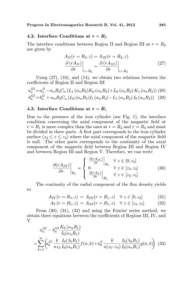
4.2. Interface Conditions at r = R2
The interface conditions between Region II and Region III at r = R2
are given by
AII (r = R2, z) = AIII (r = R2, z)∂ (rAII )
∂r
∣∣∣∣r=R2
=∂ (rAIII )
∂r
∣∣∣∣r=R2
(27)
Using (27), (10), and (14), we obtain two relations between thecoefficients of Region II and Region III
aIIIn =aII
n −αnR2Cn (L1 (αnR2)K0 (αnR2)+L0 (αnR2) K1 (αnR2)) (28)
bIIIn =bIIn + αnR2Cn (L0 (αnR2)I1 (αnR2)−L1 (αnR2) I0 (αnR2)) (29)
4.3. Interface Conditions at r = R1
Due to the presence of the iron cylinder (see Fig. 1), the interfacecondition concerning the axial component of the magnetic field atr = R1 is more complex than the ones at r = R2 and r = R3 and mustbe divided in three parts. A first part corresponds to the iron cylindersurface (z3 ≤ z ≤ z4) where the axial component of the magnetic fieldis null. The other parts corresponds to the continuity of the axialcomponent of the magnetic field between Region III and Region IVand between Region III and Region V. Therefore, we can write
∂(rAIII )∂r
∣∣∣∣R1
=
∂(rAIV )∂r
∣∣∣R1
∀ z ∈ [0, z3]
0 ∀ z ∈ [z3, z4]∂(rAV )
∂r
∣∣∣R1
∀ z ∈ [z4, z5](30)
The continuity of the radial component of the flux density yieldsto
AIV (r = R1, z) = AIII (r = R1, z) ∀ z ∈ [0, z3] (31)AV (r = R1, z) = AIII (r = R1, z) ∀ z ∈ [z4, z5] (32)
From (30), (31), (32) and using the Fourier series method, weobtain three equations between the coefficients of Regions III, IV, andV
aIIIn − bIIIn
K0 (αnR1)I0(αnR1)
=∞∑
k=1
(aIV
k
k
nz3
I0(βkR1)I0(αnR1)
f(n, k)+aVk
k
n(z5−z4)I0(λkR1)I0(αnR1)
g(n, k))
(33)

386 Lubin, Berger, and Rezzoug
aIVk =
2z3
∞∑
n=1
(aIII
n
I1 (αnR1)I1 (βkR1)
+ bIIIn
K1 (αnR1)I1 (βkR1)
)× f(n, k) (34)
aVk =
2z5 − z4
∞∑
n=1
(aIII
n
I1 (αnR1)I1 (λkR1)
+ bIIIn
K1 (αnR1)I1 (λkR1)
)× g(n, k) (35)
where
f(n, k) =
{−αn sin(kπ/2) cos(αnz3)
(α2n−β2
k)for αn 6= βk
0.5× z3 for αn = βk
(36)
g(n, k) =
{−αn cos(αnz4)
(α2n−λ2
k)for αn 6= λk
0.5× (z5 − z4) sin(αnz4) for αn = λk
(37)
Because aIIn and aIII
n are directly linked to the source term (25) and(28), we have only to solve a system of five linear equations with fiveunknowns. By rewriting the above equations in matrix and vectorsformat, a numerical solution can be found by using mathematicalsoftware (Matlab, Mathematica, etc.). It should be noted here thata numerical matrix inversion is required for the calculation of theunknown coefficients but using symbolic packages, this matrix needsto be inverted only once even in parametric studies.
5. SELF-INDUCTANCE AND ELECTROMAGNETICFORCE EXPRESSION
5.1. Electromagnetic Force Expression
The electromagnetic force acting on the iron core is obtained using theMaxwell stress tensor method. A line of radius Re and length [0, z5] inRegion III is taken as the integration path (it is also possible to choicean integration path directly around the iron core but we obtain a morecomplex analytical expression). The electromagnetic force in the axialdirection can be expressed as follows
Fz =2πRe
µ0
z5∫
0
BIIIr (Re, z)BIIIz (Re, z)dz (38)
where BIIIr and BIIIz are respectively the radial and the axialcomponents of the flux density in Region III. Their expressions canbe obtained from (14) and (23)
BIIIr (r, z) =∞∑
n=1
−αn
{aIII
n I1 (αnr) + bIIIn K1 (αnr)}
cos (αnz) (39)

Progress In Electromagnetics Research B, Vol. 41, 2012 387
BIIIz (r, z) =∞∑
n=1
αn
{aIII
n I0 (αnr)− bIIIn K0 (αnr)}
sin (αnz) (40)
Substituting (39) and (40) into (38), we obtain the followinganalytical expression for the electromagnetic force
Fz =4z5Re
µ0
∞∑
n=1
∞∑
m=1
m
m2 − n2XnYm with m 6= n (41)
andXn = −αn
{aIII
n I1 (αnRe) + bIIIn K1 (αnRe)}
Ym = αm
{aIII
m I0 (αmRe)− bIIIm K0 (αmRe)} (42)
where m and n are positive integers.
5.2. Self-inductance Expression
The self-inductance L11 of the iron-core solenoid is related to the totalstored magnetic energy as
12L11I
2 =12
∫
VA · Jdv (43)
The integral in (43) is restricted to the volume of the conductor,since the current density elsewhere is zero. We have supposed that thecurrent density is uniformly distributed over the whole cross section ofthe winding, this leads to
I =J(R3 −R2)L
N(44)
where N and I are the number of turns in the winding and the electricalcurrent in the wire, respectively. L is the axial length of the coil.
The magnetic vector potential in the winding is given by (10).Substituting (10) and (44) into (43) and integrating first in respect tothe z variable, we obtained
L11 =2πN2
(R3 −R2)2L2J
∞∑
n=1
{cos(αnz1)−cos(αnz2)
αn
×R3∫
R2
(aII
n I1 (αnr)+bIIn K1 (αnr)−CnL1 (αnr))rdr
}(45)
The radial integration in (45) leads to integral of the form:∫rI1(αnr)dr=
πr
2αn(I1(αnr)L0(αnr)−I0(αnr)L1(αnr))=
πr
2αnU(r) (46)

388 Lubin, Berger, and Rezzoug
∫rK1(αnr)dr=
πr
2αn(K1(αnr)L0(αnr)+K0(αnr)L1(αnr))=
πr
2αnV(r)(47)
∫rL1(αnr)dr=
α2nr4
6πF
(1, 2;
32,52, 3;
α2nr2
4
)=
α2nr4
6πW(r) (48)
where F in (48) is the hypergeometric function [28]. The functionsU(r), V (r) and W (r) in (46) to (48) have been introduced here tosimplify the mathematical expressions. Substituting (46), (47) and(48) into (45), the semi-analytical expression of the self-inductance isgiven by:
L11 =2πN2
(R3 −R2)2L2J
∞∑
n=1
cos(αnz1)−cos(αnz2)
2×
aIIn
πα2
n(R3U(R3)−R2U(R2))
+bIInπ
α2n
(R3V (R3)−R2V (R2))−Cn
αn3π
(R4
3W (R3)−R42W (R2)
)
(49)
An analytical expression for the self-inductance without the ironcore can be obtained by imposing the coefficients bIIIn , aIV
k , and aVk to
be null (Regions IV and V disappears without the ferromagnetic rod),that gives from (25) and (29)
aIIn = αnR3CnV (R3) bIIn = −αnR2CnU(R2) (50)
By substituting (11) and (50) into (49), we obtain an analyticalexpression for the self-inductance without the iron-core in term of aninfinite series as:
L′11 =4µ0N
2R23z
35
π(R3 −R2)2L2
∞∑
n=1,3,5...
1n4
sin2
(nπL
2z5
)
×
U(R3)V (R3)− 2R2R3
U(R2)V (R3)
+(
R2R3
)2U(R2)V (R2)
− (nR3)2
3z25
(W (R3)−
(R2R3
)4W (R2)
)
(51)
6. ANALYTICAL RESULTS AND COMPARISON WITHFINITE ELEMENT SIMULATIONS
The geometrical parameters are given in Table 1. The outer boundariesin the axial direction have been placed at z = 0 cm and z5 = 200 cm.These boundaries are sufficiently far away from the coil and the ironcore so that they do not affect the results (the length of the domain is

Progress In Electromagnetics Research B, Vol. 41, 2012 389
Figure 3. Equipotential lines around the coil for h = 7.5 cm(maximum force).
ten times bigger than the length of the coil). Analytical solutions inRegions I to V have been computed with a finite number of harmonicterms M and K as indicated in Table 1.
In order to validate the proposed model, the analytical results havebeen compared with those obtained by using a finite element (FE)software FEMM [30]. For the FE solutions, a relative permeabilityof µr = 10000 has been used for the iron core. The axial length ofthe whole domain in FE simulations is the same as the one of theanalytical model. Homogeneous Dirichlet boundary conditions havebeen imposed at z = 0 and z = z5 for FE simulations like for theanalytical model. The mesh in the different regions has been refineduntil convergent results are obtained.
Figure 3 shows the equipotential lines around the coil when thecenter of the iron core is placed at a distance h = 7.5 cm from thecenter of the coil. This position corresponds to the maximum forceacting on the iron core as it can be observed in Fig. 5.
The radial and axial components of the magnetic flux densitydistribution along the z-axis in Region III are shown in Fig. 4. The fluxdensity distribution without the iron core is also plotted in this figure(when the iron core is not present, the solution is symmetric about thecenter of the coil). The results without the iron core are obtained withthe analytical model by imposing the coefficients bIIIn , aIV
k , and aVk to
be null.From Fig. 4, the effects of the iron core on the magnetic field
distribution are very clear. One can see the distortion of the fluxdensity waveforms at the vicinity of the iron cylinder. An excellent

390 Lubin, Berger, and Rezzoug
agreement with the results deduced from FEM is obtained.Figure 5 compares the electromagnetic axial force acting on the
iron core obtained with the semi-analytical formula (41) and withFE simulations. For the computation, the center of the iron core isdisplaced axially by a distance h relative to the center of the coil. Asexpected, the force is null when the iron core is centered inside thecoil and it presents a symmetry around h = 0. The maximum force isreached for a displacement h = 7.5 cm and its value is equal to 76.8 Nwith the analytical model and 77.9 N with FEM. The error is less than1.5% if we considered 50 harmonic terms. It appears that results fromthe proposed analytical method and FE simulations are very close toeach other. To compute the peak value of the force, the computationtime is 1.21 s with the analytical model (50 harmonic terms, ProcessorIntel Core2 Duo P8700, 2.53 GHz, Matlab Software) whereas the finiteelement simulation takes 5.83 s for a mesh of 97 423 elements [30]. The
(a) (b)
Figure 4. Radial (a) and axial (b) components of the flux density inRegion III for r = 4 cm and h = 7.5 cm.
Figure 5. Electromagnetic force versus iron-core position h.

Progress In Electromagnetics Research B, Vol. 41, 2012 391
Table 1. Geometrical parameters.
Symbol Quantity valueR1 Radius of the iron core 3 cmR2 Inner radius of the coil 5 cmR3 Outer radius of the coil 7 cmz1 Axial position of the coil (left side) 90 cmz2 Axial position of the coil (right side) 110 cmL Axial length of the coil (L = z2 − z1) 20 cmN Number of turns in the winding 1000
hAxial position of the center of
the iron core from the center of the coilvariable
z3 Axial position of the iron core (left side) 95 + h cmz4 Axial position of the iron core (right side) 105 + h cml Axial length of the iron core (l = z4 − z3) 10 cmz5 Outer boundary of the domain 200 cmJ Current density in the coil 5 A/mm2
MNumber of harmonic terms used for magnetic
field calculation in Regions I, II and III50
KNumber of harmonic terms used for magnetic
field calculation in Regions IV and V50
analytical computation being much faster, the presented model canadvantageously be used in a preliminary design stage.
Figure 6 gives the self-inductance variation versus iron rodposition obtained with the semi-analytical formula (49) and with FEsimulations. As for the magnetic force, the iron core is displaced axiallyby a distance h relative to the center of the coil. As expected, the self-inductance is maximal for h = 0 cm and presents a symmetry aroundh = 0 cm. The maximal value of the self-inductance is L11 = 85.8 mHwith the analytical model (50 harmonic terms) and L11 = 87 mH withfinite element simulations (97 423 elements). The error is less than1.4%. The value of the self-inductance without the iron core (51)is L′11 = 48.8mH by using the analytical model (50 harmonics) andL′11 = 49mH with finite element simulations. Without the ironcylinder (51), the error on the self-inductance computation is lessthan 0.4% and the computational time is much faster (0.11 s for 50harmonic terms). The analytical expressions for the self-inductancewith or without iron core are well verified by comparison with finite

392 Lubin, Berger, and Rezzoug
Figure 6. Self-inductance versus iron-core position h.
(a) (b)
Figure 7. Performances of the analytical model versus the number ofharmonic terms; (a) Error; (b) Computer time.
element simulations.The error (axial force and self-inductance values) and computer
time variations with respect to the number of harmonic termsconsidered in evaluating the analytical solutions are given in Table 2and are shown in Fig. 7(a) and Fig. 7(b). The same number ofharmonic terms is considered for the five regions (M = K). Forthe definition of the error, we assumed that results obtained withfinite element simulations are correct (F = 77.9 N and L11 = 87 mH).Only the peak values of the force (h = 7.5 cm) and self-inductance(h = 0 cm) are considered here. As shown in Fig. 7, the error increasesand the computer time decreases when the number of harmonic termsdecreases. We can observe from Fig. 7(a) that the error is smaller forthe self-inductance than for the force. From Table 2, we can say thata number of 40 harmonic terms in the analytical model seems to bea good compromise in terms of precision and computer time for thestudied example.
Progress In Electromagnetics Research B, Vol. 41, 2012 393
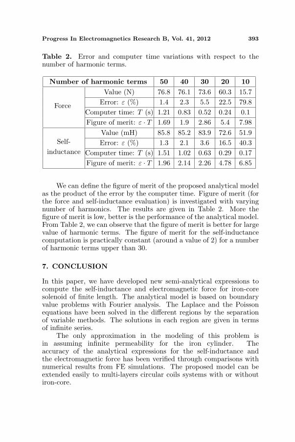
Table 2. Error and computer time variations with respect to thenumber of harmonic terms.
Number of harmonic terms 50 40 30 20 10
Force
Value (N) 76.8 76.1 73.6 60.3 15.7Error: ε (%) 1.4 2.3 5.5 22.5 79.8
Computer time: T (s) 1.21 0.83 0.52 0.24 0.1Figure of merit: ε · T 1.69 1.9 2.86 5.4 7.98
Self-inductance
Value (mH) 85.8 85.2 83.9 72.6 51.9Error: ε (%) 1.3 2.1 3.6 16.5 40.3
Computer time: T (s) 1.51 1.02 0.63 0.29 0.17Figure of merit: ε · T 1.96 2.14 2.26 4.78 6.85
We can define the figure of merit of the proposed analytical modelas the product of the error by the computer time. Figure of merit (forthe force and self-inductance evaluation) is investigated with varyingnumber of harmonics. The results are given in Table 2. More thefigure of merit is low, better is the performance of the analytical model.From Table 2, we can observe that the figure of merit is better for largevalue of harmonic terms. The figure of merit for the self-inductancecomputation is practically constant (around a value of 2) for a numberof harmonic terms upper than 30.
7. CONCLUSION
In this paper, we have developed new semi-analytical expressions tocompute the self-inductance and electromagnetic force for iron-coresolenoid of finite length. The analytical model is based on boundaryvalue problems with Fourier analysis. The Laplace and the Poissonequations have been solved in the different regions by the separationof variable methods. The solutions in each region are given in termsof infinite series.
The only approximation in the modeling of this problem isin assuming infinite permeability for the iron cylinder. Theaccuracy of the analytical expressions for the self-inductance andthe electromagnetic force has been verified through comparisons withnumerical results from FE simulations. The proposed model can beextended easily to multi-layers circular coils systems with or withoutiron-core.

394 Lubin, Berger, and Rezzoug
REFERENCES
1. Garrett, M. W., “Calculations of fields, forces and mutualinductances of current systems by elliptic integral,” J. Appl. Phys.,Vol. 34, 2567, 1963.
2. Durand, E., Magnetostatique, Masson et Cie, Paris, 1968.3. Urankar, L., “Vector potential and magnetic field of current-
carrying finite arc segment in analytical form, part III: Exactcomputation for rectangular cross-section,” IEEE Trans. Magn.,Vol. 18, No. 6, 1860–1867, Nov. 1982.
4. Yu, D. and K. S. Han, “Self-inductance of aire-core circular coilswith rectangular cross-section,” IEEE Trans. Magn., Vol. 43,No. 6, 3916–3921, Nov. 1987.
5. Rezzoug, A., J. P. Caron, and F. M. Sargos, “Analyticalcalculation of flux induction and forces of thick coils with finitelength,” IEEE Trans. Magn., Vol. 28, No. 5, 2250–2252, Sep. 1992.
6. Azzerboni, B., E. Cardelli, M. Raugi, A. Tellini, and G. Tina,“Magnetic field evaluation for thick annular conductors,” IEEETrans. Magn., Vol. 29, No. 3, 2090–2094, May 1993.
7. Conway, J. T., “Exact solutions for the magnetic fields of solenoidsand current distributions,” IEEE Trans. Magn., Vol. 37, No. 4,2977–2988, Jul. 2001.
8. Babic, S. and C. Akiel, “Improvement of the analytical calculationof the magnetic field produced by permanent magnet rings,”Progress In Electromagnetic Research C, Vol. 5, 71–82, 2008.
9. Conway, J. T., “Trigonometric integrals for the magnetic field ofthe coil of rectangular cross section,” IEEE Trans. Magn., Vol. 42,No. 5, 1538–1548, May 2006.
10. Babic, S. and C. Akyel, “Magnetic force calculation between thincoaxial circular coils in air,” IEEE Trans. Magn., Vol. 44, No. 4,445–452, Apr. 2008.
11. Conway, J. T., “Inductance calculations for circular coils ofrectangular cross section and parallel axes using Bessel and Struvefunctions,” IEEE Trans. Magn., Vol. 46, No. 1, 75–81, Jan. 2010.
12. Ravaud, R., G. Lemarquand, V. Lemarquand, and C. Depollier,“The three exact components of the magnetic field createdby a radially magnetized tile permanent magnet,” Progress InElectromagnetics Research, Vol. 88, 307–319, 2008.
13. Ravaud, R., G. Lemarquand, V. Lemarquand, S. Babic, andC. Akyel, “Mutual inductance and force exerted between thickcoils,” Progress In Electromagnetics Research, Vol. 102, 367–380,

Progress In Electromagnetics Research B, Vol. 41, 2012 395
2010.14. Babic, S., F. Sirois, C. Akyel, G. Lemarquand, V. Lemarquand,
and R. Ravaud, “New formulas for mutual inductance and axialmagnetic force between a thin wall solenoid and a thick circularcoil of rectangular cross-section,” IEEE Trans. Magn., Vol. 47,No. 8, 2034–2044, Aug. 2011.
15. Zhang, D. and C. S. Koh, “An efficient semi-analytic computationmethod of magnetic field for a circular coil with rectangular crosssection,” IEEE Trans. Magn., Vol. 48, No. 1, 62–68, Jan. 2012.
16. Gysen, B. L. J., K. J. Meessen, J. J. H. Paulides, andE. A. Lomonova, “General formulation of the electromagnetic fielddistribution in machines and devices using Fourier analysis,” IEEETrans. Magn., Vol. 46, No. 1, 39–52, Jan. 2010.
17. Lubin, T., S. Mezani, and A. Rezzoug, “Exact analytical methodfor magnetic field computation in the air-gap of cylindricalelectrical machines considering slotting effects,” IEEE Trans.Magn., Vol. 46, No. 4, 1092–1099, Apr. 2010.
18. Rabins, L., “Transformer reactances calculation with digitalcomputer,” AIEE Trans., Vol. 75, Pt. I, 261–267, Jul. 1956.
19. Martinelli, G. and A. Morini, “A potential vector field solution insuperconducting magnets, part I: Method of calculation,” IEEETrans. Magn., Vol. 19, No. 4, 1537–1545, Jul. 1983.
20. Caldwell, J. and A. Zisserman, “A Fourier series approach tomagnetostatic field calculations involving magnetic materials,” J.Appl. Phys., Vol. 54, No. 9, 4734–4738, Sep. 1983.
21. Caldwell, J. and A. Zisserman, “Magnetostatic field calculationsinvolving iron using eigenfunction expansion,” IEEE Trans.Magn., Vol. 19, No. 6, 2725–2729, Nov. 1983.
22. Uzal, E., I. Ozkol, and M. O. Kaya, “Impedance of acoil surrounding an infinite cylinder with an arbitrary radialconductivity profile,” IEEE Trans. Magn., Vol. 34, No. 1, 213–217, Nov. 1987.
23. Wilcox, D. J., M. Conlon, and W. G. Hurley, “Calculation ofself and mutual impedances for coils on ferromagnetic cores,” IEEProceedings, Vol. 135, Pt. A, No. 7, 470–476, Jan. 1998.
24. Dodd, C. V. and W. E. Deeds, “Analytical solutions to eddy-current probe-coil problems,” Journal of Applied Physics, Vol. 39,2829–2838, May 1968.
25. Dodd, C. V., C. C. Cheng, and W. E. Deeds, “Induction coilscoaxial with an arbitrary number of cylindrical conductors,”Journal of Applied Physics, Vol. 45, 638–647, Feb. 1974.
396 Lubin, Berger, and Rezzoug
26. Bowler, J. R. and T. P. Theodoulidis, “Eddy currents inducedin a conducting rod of finite length by a coaxial encircling coil,”Journal of Physics D: Applied Physics, Vol. 38, 2861–2868, 2005.
27. Sun, H., J. R. Bowler, and T. P. Theodoulidis, “Eddy currentsinduced in a finite length layered rod by a coaxial coil,” IEEETrans. Magn., Vol. 41, No. 9, 2455–2461, Sep. 2005.
28. Abramowitz, M. and I. A. Stegun, Handbook of MathematicalFunctions, Dover Publications, Inc., New York, 1972.
29. Farlow, S. J., Partial Differential Equations for Scientists andEngineers, 414, Dover Publications, New York, 1993.
30. Meeker, D. C., Finite Element Method Magnetics, Version 4.2,Apr. 1, 2009, http://www.femm.info.