inductive communication and localization method for

Inductive Communication and Localization Method for Wireless Sensors in

Photobioreactors

SENSORCOMM 2020

Presenter: David Demetz

[email protected]

Institute of Measurement and Sensor Technology

UMIT Tirol – The Tyrolean Private University

Hall in Tirol, Austria

November 21 - November 25, 2020

Authors: David Demetz, Alexander Sutor

David Demetz was born in South-Tirol, Italy, in

1994. He received the Dipl.-Ing. degree in

Mechatronics from the Umit Tirol, Hall in Tirol,

Austria and the University of Innsbruck, Austria

(Joint Degree Programme), in 2019.

In 2019 he joined the Institute of Measurement and

Sensor Technology, at the Umit Tirol, Austria. His

research interests include wireless sensors,

inductive coupling systems and signal processing.

Content

Photoreactors in general and the internal illumination of them

Inductive communication method for wireless sensors

Inductive sensor localization: theory and results

Simulation: localization accuracy improvement by using multiple receivers

SENSORCOMM 2020 3D. Demetz, A. Sutor November 2020

Photoreactors in general

Are used to

cultivate photosynthetic active microorganismsand cells

to perform photocatalytic reactions

General problem:

limited penetration depth of light

4D. Demetz, A. Sutor November 2020SENSORCOMM 2020

Internally illuminated photoreactors

Wireless light emitters (WLE)



Inductively supplied spherical light emitters (WLEs) which are floating in the reactor media

The driving Coils at the outer circumference of the reactor are driven by a class-e power amplifier


The next step:

inclusion of sensors for measuring crucial parameters

e.g. temperature, pH-value, oxygen and carbon dioxide concentrations, …

wireless sensors to counteract the drawback of measuring the respective parameter only at one point in the reactor

determining the position of the sensor leads to a spatial resolution of the measured parameter


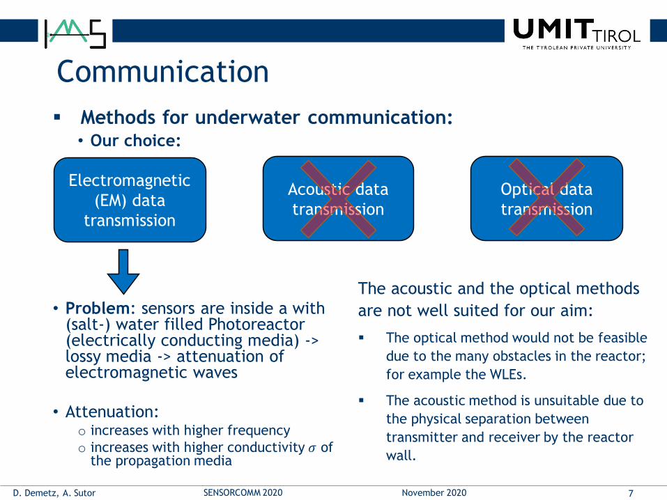
Communication

Methods for underwater communication:• Our choice:

Electromagnetic

(EM) data

transmission

Acoustic data

transmission

Optical data

transmission

• Problem: sensors are inside a with(salt-) water filled Photoreactor (electrically conducting media) -> lossy media -> attenuation of electromagnetic waves

• Attenuation:o increases with higher frequency

o increases with higher conductivity 𝜎 of the propagation media


The acoustic and the optical methods

are not well suited for our aim:

The optical method would not be feasible

due to the many obstacles in the reactor;

for example the WLEs.

The acoustic method is unsuitable due to

the physical separation between

transmitter and receiver by the reactor

wall.

Communication

Physical requirements for the communication layer:

• low frequencies

• based on the inductive principle since the relative magnetic permeability of water (and saltwater) is ≈ 1 (like air).

Our choice: inductive communication link with a carrier frequency of 298kHz -> only the quasi-static field component results relevant

• On-off keying is used as a modulation technique.


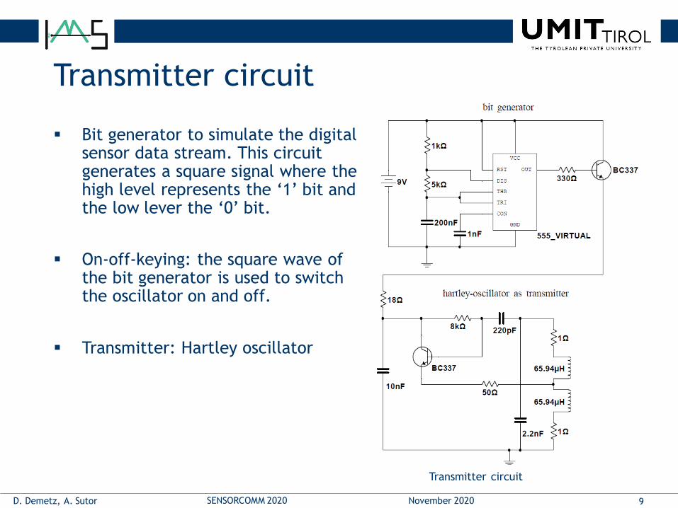
Transmitter circuit

Bit generator to simulate the digital sensor data stream. This circuit generates a square signal where the high level represents the ‘1’ bit and the low lever the ‘0’ bit.

On-off-keying: the square wave of the bit generator is used to switch the oscillator on and off.

Transmitter: Hartley oscillator

Transmitter circuit


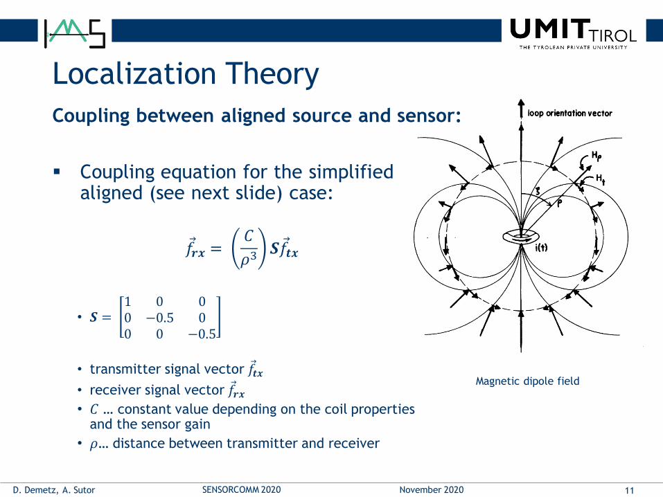
Localization Theory

For the localization task we use the magnetic dipole field equation to model the magnetic field of the transmitter coil

• Magnetic field strength in radial 𝐻ρ

and tangential 𝐻𝑡 component

𝐻ρ =𝑁𝐼𝐴

2𝜋ρ3cos 𝜍

𝐻𝑡 =𝑁𝐼𝐴

4𝜋ρ3sin 𝜍

Magnetic dipole field

Measuring the magnetic field at well defined positions outside the reactor makes the calculation of the transmitter positionpossible.


Localization Theory

Coupling equation for the simplified aligned (see next slide) case:

Ԧ𝑓𝒓𝒙 =𝐶

𝜌3𝑺 Ԧ𝑓𝒕𝒙

• 𝑺 =1 0 00 −0.5 00 0 −0.5

• transmitter signal vector Ԧ𝑓𝒕𝒙

• receiver signal vector Ԧ𝑓𝒓𝒙• 𝐶 … constant value depending on the coil properties

and the sensor gain

• 𝜌… distance between transmitter and receiver

11

Coupling between aligned source and sensor:

Magnetic dipole field

D. Demetz, A. Sutor November 2020SENSORCOMM 2020

Localization Theory

12

Coupling between aligned source and sensor:

Alignment conditions:

Ԧ𝑒𝑥−𝑟𝑥 = Ԧ𝑒𝑥−𝑡𝑥

Ԧ𝑒𝑦−𝑟𝑥 || Ԧ𝑒𝑦−𝑡𝑥

Ԧ𝑒𝑧−𝑟𝑥 || Ԧ𝑒𝑧−𝑡𝑥


Alignement conditions

13

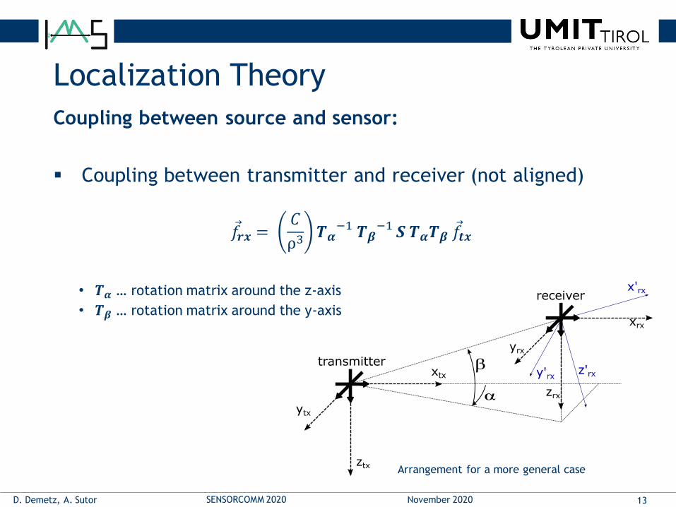
Localization Theory

Coupling between source and sensor:

Coupling between transmitter and receiver (not aligned)

Ԧ𝑓𝒓𝒙 =𝐶

ρ3𝑻𝜶

−1 𝑻𝜷−1 𝑺 𝑻𝜶𝑻𝜷 Ԧ𝑓𝒕𝒙

• 𝑻𝜶 … rotation matrix around the z-axis

• 𝑻𝜷 … rotation matrix around the y-axis


Arrangement for a more general case

Localization Theory

Two receivers for measuring the magnetic field at a defined positions.

Solving the equation

𝑻𝜶−1 𝑻𝜷

−1 𝑺 𝑻𝜶𝑻𝜷 Ԧ𝑓𝒕𝒙 − Ԧ𝑓𝒓𝒙 = 𝟎

with Ԧ𝑓𝒕𝒙 = (𝟎 𝟎 𝒂)𝑻 for the angles α and β (and for a) enables the calculation of a directional vector Ԧ𝑟 which points from themeasurement point to the transmitter position.

The position is calculated by determining the point where the two directional vectors come closest (ideally the intersection).

14

Our method


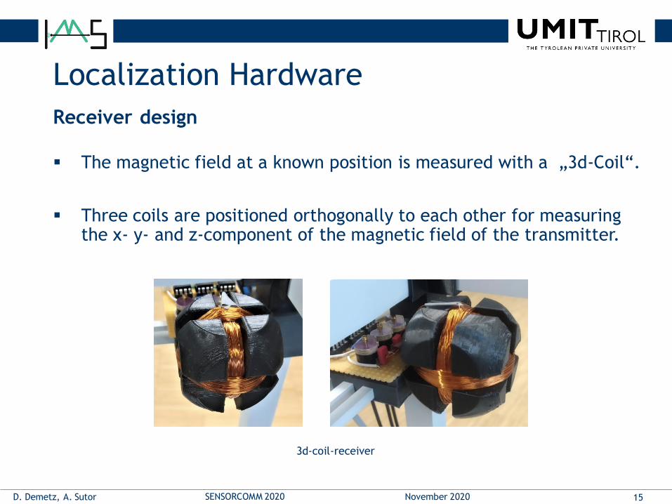
Localization Hardware

The magnetic field at a known position is measured with a „3d-Coil“.

Three coils are positioned orthogonally to each other for measuring the x- y- and z-component of the magnetic field of the transmitter.

3d-coil-receiver

15

Receiver design



Coil as main receiver component.

The coil signal is amplified with a resonant filter in order to amplify the receiver signal only at the transmitting frequency.

16

Receiver design

Resonant filter



Bode magnitude plot of the resonant filter:

17

Receiver design


Localization Setup

18

Our system

With the measured magnetic field and based on the magnetic dipole equation a

directional vector റ𝑟 is calculated for each receiver. This vector points from the

receiver to the transmitter.

The directional vector റ𝑟 is defined by the two angles α and β.

By using two or more receivers the transmitter position is calculated by finding

the point were the direction vectors comes closest, ideally the intersection.


Definition of the directional vector റ𝑟

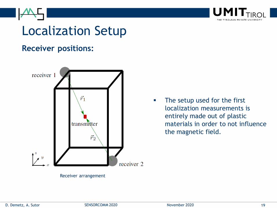
Localization Setup

19

Receiver positions:

Receiver arrangement


The setup used for the first

localization measurements is

entirely made out of plastic

materials in order to not influence

the magnetic field.

Localization Measurements

20

Measurement points:

Five measuring points at seven different heights in our region of interest.

The x and y coordinates of the individual points are the same at all heights.

Measurement pattern (unit: cm)


Results

Real position vs. measured position (25cm height)


Results

Mean values of the relative errors of all three coordinates at different heights


For low as well as for high z-coordinates, the distance to one receiver increases and, therefore, the accuracy decreases.

Simulation results

Accuracy improvement by using more than two receivers

• Mean value of the magnitude of the deviation vectors between the exact

positions and calculated positions with added noise.


signal amplitude variation:• random values in the range between 0

and 5% of the calculated exact amplitude

overlap of white noise• random values in the range between 0

and 50% of the signal amplitude

power supply magnetic field overlap• random values in the range between 0

and 50% of the signal amplitude

Thank you for your attention!

24November 2020SENSORCOMM 2020D. Demetz, A. Sutor

References

M. Heining, A. Sutor, S. Stute, C. Lindenberger und R. Buchholz, „Internal illumination of photobioreactors via wireless light emitters:,“ Journal of Applied Phycology, vol. 27, pp. 59-66, 2015, doi:10.1007/s10811-014-0290-x.

A. Sutor, M. Heining und R. Buchholz, „A Class-E Amplifier for a Loosely Coupled Inductive Power,“ Energies, Bd. 12, Nr. 6, 2019, doi: 10.3390/en12061165.

B. O. Burek, A. Sutor, B. W. Bahnemann und J. Z. Bloh, „Completely integrated wirelessly-powered photocatalyst-coated spheres as a novel means to perform heterogeneous photocatalytic reactions,“ Catal. Sci. Technol., Bd. 7, Nr. 21, p. 4977–4983, 2017, doi: 10.1039/c7cy01537b.

J. Edelmann, R. Stojakovic, C. Bauer und T. Ussmueller, „An Inductive Through-The-Head OOK Communication Platform for Assistive Listening Devices,“ 2018 IEEE Topical Conference on Wireless Sensors and Sensor Networks (WiSNet), p. 30–33, 2018, doi: 10.1109/WISNET.2018.8311556.

F. H. Raab, E. B. Blood, T. O. Steiner und H. R. Jones, „Magnetic position and orientation tracking system,“ IEEE Transactions on Aerospace and Electronic Systems, p. 709–718, 1979, doi: 10.1109/TAES.1979.308860.

C. A. Balanis „Advanced Engineering Electromagnetics” John Wiley & Sons, 2012 ISBN: 0470589485, 9780470589489


inductive communication and localization method for

Documents