industrial applications of digital rock technology
TRANSCRIPT

1
Industrial applications of digital rock technology
Carl Fredrik Berg1*, Olivier Lopez1 and Håvard Berland1
1 Statoil R&D Center, Arkitekt Ebbels veg 10, Rotvoll, 7053 Trondheim, Norway
* Corresponding author’s email address: [email protected]. Present address: Department of
Geoscience and Petroleum, NTNU, Trondheim, Norway.
Abstract
This article provides an overview of the current state of digital rock technology, with emphasis on
industrial applications. We show how imaging and image analysis can be applied for rock typing
and modeling of end-point saturations. Different methods to obtain a digital model of the pore
space from pore scale images are presented, and the strengths and weaknesses of the different
methods are discussed. We also show how imaging bridges the different subjects of geology,
petrophysics and reservoir simulations, by being a common denominator for results in all these
subjects. Network modeling is compared to direct simulations on grid models, and their
respective strengths are discussed. Finally we present an example of digital rock technology
applied to a sandstone oil reservoir. Results from digital rock modeling are compared to results
from traditional laboratory experiments. We highlight the mutual benefits from conducting both
traditional experiments and digital rock modeling.
Keywords: Digital rock, pore scale, imaging, modeling, simulation.
1 Contents 2 Introduction ............................................................................................................................. 2
3 Imaging .................................................................................................................................... 5
3.1 3D imaging ...................................................................................................................... 5
3.2 2D imaging ...................................................................................................................... 7
3.3 3D reconstruction from 2D images ................................................................................. 8
4 Image analysis ......................................................................................................................... 9

2
4.1 Mineralogy ...................................................................................................................... 9
4.2 Porosity classification .................................................................................................... 10
4.2.1 Effective porosity .................................................................................................. 11
4.2.2 Microporosity ........................................................................................................ 12
4.2.3 Irreducible water saturation ................................................................................... 14
4.3 Grain size and distribution ............................................................................................. 15
5 Simulation ............................................................................................................................. 19
5.1 Absolute and relative permeability ................................................................................ 19
5.2 Electrical conductance and steady-state diffusion ......................................................... 20
5.3 Elastic properties ........................................................................................................... 21
6 Application example .............................................................................................................. 21
7 Summary ............................................................................................................................... 27
8 Bibliography .......................................................................................................................... 28
2 Introduction
Information about subsurface reservoir characteristics can roughly divided into two classes; data
obtained from surface surveys such as seismic, electromagnetic, gravimetric etc., and data
obtained from wells, such as well logs, transient pressure testing, reservoir performance, cores
and drill cuttings. While data obtained from the surface typically have low resolution and large
coverage, well data typically has high resolution and low coverage. At the extreme, core material
can provide pore scale resolution, the foundation for digital rock physics, as will be discussed in
detail in this article.
Cores provides essential data for formation evaluation, with direct information on the presence,
distribution and transport of reservoir fluids at a peerless resolution (Andersen et al., 2013).
Conventional core analysis (CCA) provides basic properties such as porosity, permeability and
grain density, while special core analysis (SCAL) provides more complex reservoir properties
such as capillary pressure, relative permeability and electrical properties (McPhee et al., 2015).
Digital rock physics is integrated with and provides similar types of data as CCA and SCAL, and
consequentially has a similar entry point into conventional subsurface workflows as CCA and
SCAL. However, the strong modeling component of digital rock physics brings it closer to
reservoir modeling than traditional CCA and SCAL.
Digital rock physics (DRP) is to numerically solve transport equations on digital representations
of rock samples. This roughly divides digital rock technology into two parts: imaging and
modeling (Andrä et al., 2013a, 2013b; Blunt et al., 2013). The aim of digital rock physics is thus
to derive a digital description of a reservoir rock, and then perform numerical simulations of
transport processes on this obtained digital structure. It could be argued that digital image
analysis is a prerequisite for digital rock physics, whereas digital rock physics only comprises

3
simulation of rock physics. Such a distinction would classify the calculation of porosity as digital
image analysis, while obtaining the permeability by solving the Stokes equation on a segmented
rock image would classify as digital rock physics. Such a distinction have advantages, however
imaging and simulations are so intertwined that this article will classify both as digital rock
physics.
Traditional workflows for rock physics are typically based on purely empirical relations from
laboratory experiments, e.g. Archie’s law (Archie, 1942). Theoretical models based on simplified
microstructures and calibrated to laboratory data is also commonly used, e.g. the Kozeny-Carman
relationship (Carman, 1937; Kozeny, 1927). There are limitations for the number of different data
types that can be measured on a single rock sample with traditional laboratory experiments. In
contrast, any effective property that can be calculated with digital rock modeling can be
calculated on the same pore structure, i.e. the same sample (Arns et al., 2005). This removes a
major uncertainty for cross-property relations: The assumed similarity of sister-plugs. Further,
digital rock physics opens up new possibilities to link effective properties to the underlying pore
structure, and thereby obtain fundamental cross-property relations (Berg and Held, 2016).
Furthermore, pore scale characterization of two-phase flow can lead to fundamental
understanding of macroscopic parameters such as relative permeability (Liu et al., 2017).
Calculation of transport properties on digital representations of the pore structure are typically
fast compared to laboratory experiments. Calculation of different properties can be conducted in
parallel, thus enabling a further acceleration compared to laboratory experiments if the same plug
is planned to be used serially in several experiments. In summary, digital rock physics has the
possibility to reduce uncertainty in formation evaluation by providing fundamental rock physics
relations at a reduced time.
Digital rock physics typically require imaging and modeling at high resolution and large coverage
(Andrä et al., 2013a, 2013b). Due to limitations on imaging and computational power, the advent
of digital rock technology was mostly devoted to basic research on transport and displacement
processes on simplified pore structures or on clean well-sorted outcrop rock samples.
Improvements in imaging and computational power has enabled application of digital rock
physics on ever more complex rock samples. Such improvements has transformed the application
of digital rock technology from mostly being devoted to basic research to an integrated element in
(oil-)industry workflows for modeling of transport in porous media (Blunt et al., 2013; Fredrich et
al., 2014; Lopez et al., 2012, 2010).
The obtainable properties from digital rock physics can be divided into three classes. The first
class is mainly dependent on an accurate description of the pore structure. With an accurate three-
dimensional (3D) pore structure description one can obtain conventional core analysis single-
phase properties such as porosity and permeability (Berg, 2014; Øren et al., 2007; Schwartz et al.,
1993). Also the formation factor is mainly dictated by the pore structure, however it should be
noted that formation factor could be significantly influenced by clays and surface conductance
(Berg, 2012; Johnson et al., 1986; Wildenschild et al., 2000). The second class is multiphase
properties with simple fluid-fluid and fluid-rock interactions, such as capillary dominated primary
drainage. This includes properties such as primary drainage capillary pressure (including mercury
injection) and saturation (electrical resistivity) index (Bekri et al., 2003; C. F. Berg et al., 2016;
Gomari et al., 2011). The third class has complex rock-fluid and fluid-fluid interactions, such as
relative permeability and imbibition capillary pressure (Øren et al., 1998; Ramstad et al., 2010;
Valvatne and Blunt, 2004).
The two first classes of digital rock results are thus mainly influenced by the digital
representation of the pore structure, while the third class additionally needs accurate information
on fluid-fluid and fluid-rock interactions. These two types of input translates into the two main
challenges for digital rock physics.

4
The first is to obtain 3D information which resolves the pore structure to a sufficient degree, and
then to balance the opposing objectives of sufficient resolution with a representative elementary
volume (REV) (Al-Raoush and Papadopoulos, 2010). This challenge is strongly dependent on the
sample; clean sands with small grain size variation is demonstrated feasible today, while larger
grain size variation, cementation, clays and partly dissolved grains still pose significant problems.
Advances in imaging has been an integral part of the growth of digital rock modeling, and has to
some extent solved the challenge of obtaining pore structure data of sufficient resolution. Larger
images translate into computational challenges; modeling and simulations with sufficient
resolution at a REV is computational heavy. This challenge is commonly targeted by brute force
and parallel computing, while dynamic gridding, network modeling, hybrid solutions and
upscaling are other ways to tackle the same issue.
The second main challenge for digital rock physics is how to implement fluid-fluid and fluid-rock
interactions. These properties are translated into interfacial tension, wettability and contact
angles, thus one need interfacial tension, wettability and a contact angle distribution
representative for the reservoir in question (Sorbie and Skauge, 2012). The fluid-fluid property
interfacial tension is fairly straightforward to measure and to implement into simulators. For the
fluid-rock properties, there is a range of methods to include wettability and contact angle
descriptions into pore scale multiphase simulations (Blunt, 1998; Øren et al., 1998; Valvatne and
Blunt, 2004). Thus the challenge is not a lack of flexibility when including fluid-rock interaction
into the simulations, but how to decide on a representative description. There exist fairly simple
measurement methods for fluid-rock properties, such as measuring the contact angle of a droplet
on a surface. Unfortunately it is not simple to implement the experimental results into pore scale
simulators with a complex surface geometry and a range of mineral surfaces. An even harder
problem, which is shared with traditional experiments, is to relate the fluid-rock properties to
reservoir properties. Typically this is solved by ageing rock samples in crude oil from the relevant
oil reservoir. It is assumed that the rock surface then changes wettability to a state that resembles
reservoir conditions. The fluid configuration at such a wettability state can be imaged, both in
micro-tomography (micro-CT) and with scanning electron microscopes (SEM). Contact angles
can be measured directly by imaging, at least for samples were one of the fluids is strongly
wetting (Andrew et al., 2014). Unfortunately, such advanced imaging cannot answer the
underlying problem: Is the obtained wettability state representative for the reservoir in question.
As digital rock models are many orders of magnitude smaller than a grid block in a reservoir
simulation model, bringing digital rock results into a full field reservoir simulation involves
upscaling (Aarnes et al., 2007; Lohne et al., 2006). This is a challenge digital rock modeling
shares with experimental results from core samples: Relative to the size of grid blocks in
reservoir models the size of core samples and digital rock models are essentially the same. As
geological structures might contain laminas smaller than the size of core plugs, flow parameters
obtained from core flooding does not always correspond to a REV (Bhattad et al., 2014; Nordahl
and Ringrose, 2008). Digital rock modelling can easily accommodate different model sizes, and
thereby ensure the flow parameters are representative for a REV (Nordahl et al., 2014; Odsæter et
al., 2015).
Digital rock physics has been applied to a variety of sedimentary rocks. Arguably, digital rock
physics has been centered on siliciclastic rocks. The advent of the technology focused on outcrop
samples (Arns et al., 2001; Bakke and Øren, 1997; Schwartz et al., 1994), while subsequent
studies has been extended to reservoir rocks (Lopez et al., 2010; Øren et al., 2007). Carbonates,
the second most abundant rock type for oil reservoirs, has also been studies from the onset of
digital rock physics (Schwartz et al., 1994), with later uptake for industrial applications (Grader et
al., 2010; Kalam et al., 2012; Lopez et al., 2012). It should be noted that large pore size variations
in carbonates might require multiscale modeling (Biswal et al., 2009; Lopez et al., 2012). The
arrival of the shale hydrocarbon industry has delivered a third class of reservoir rocks investigated

5
by digital rock physics. Recently a majority of cored wells in the US are from shale reservoirs,
making shale an important rock type for core analysis (Walls and Armbruster, 2012). The
extremely small pore sizes in such samples make them intrinsically hard to resolve and model
(Kelly et al., 2016). However, as such samples are equally hard to measure using traditionally
laboratory procedures, digital rock physics has been a popular choice for evaluating shale samples
(Walls et al., 2012).
This article starts with an overview of different imaging techniques and 3D reconstruction that
has been applied in digital rock technology. Section 4 presents methods and results from image
analysis, including direct industrial applications of image analysis results. In Section 5 we present
different pore scale simulation methods, with a focus on the direct modeling versus network
modeling. An application of digital rock technology is presented in Section 6, while we
summarize this article in the last section, Section 7.
3 Imaging
In digital rock physics workflows, imaging of rock samples typically has a two-fold purpose: The
first is to obtain sample description such as grain size distribution, pore size distribution,
mineralogy, clay content etc. The other purpose is to obtain 3D structures for computation of
effective properties such as permeability and conductivity. Those two imaging purposes cause
different constraints, some of which are conflicting.
At the early stage of digital rock physics it was more common to reconstruct 3D structures from
2D electron microscopy images than to use 3D X-ray tomography images directly. This was due
to the low quality and low availability of X-ray tomography at the resolution needed for
predictive modeling. As X-ray tomography is of better quality and more readily available today, it
is more frequently used. However, there are situations where the advantages from starting with
2D images make this method preferable also today.
3.1 3D imaging
X-ray computed tomography (CT) reconstructs a 3D image of a sample from a set of X-ray
images of the sample taken at different angles (Wildenschild and Sheppard, 2013). CT-imaging
has been used in the oil industry for decades (Cromwell et al., 1984). Typical use includes core
inspection, localization of where to drill plug samples, inspection of core plugs, imaging of core
flooding experiments and rock characterization (Gilliland and Coles, 1990; Honarpour et al.,
1985; Hove et al., 1987; Wellington and Vinegar, 1987). For such applications it is common to
use a medical CT scanner. In medical CTs the X-ray source and detectors are rotating around the
stationary sample.
Calculation of effective rock properties from digitized images of the pore structure requires an
image resolution that sufficiently resolves all parts of the structure important for the property in
question. Digital rock physics therefore requires a higher image resolution that what is obtained
using standard medical CTs. Some of the first high-resolution images of rock samples were
acquired using the beam-line at a synchrotron facility as the X-ray source (Flannery et al., 1987).
Today, imaging using synchrotrons are mostly conducted when one wants to capture rapid
transient processes on the pore scale (Berg et al., 2013).

6
Laboratory based micro-CT equipment are readily available today, and is the standard equipment
for obtaining 3D images of rock samples for digital rock physics (Wildenschild and Sheppard,
2013). Most such laboratory micro-CTs use a stationary X-ray source and detector while the
sample is rotated, however micro-CT gantry scanners are also used (Bultreys et al., 2015).
As stated, when imaging for digital rock analysis one needs to resolve the structure important for
the property of interest. Exemplary, the main flow paths are of ultimate importance for
calculation of flow properties, while electrical properties is dependent on all porosity, also the
microporosity to be discussed in Subsection 4.2.2.
Further, the 3D distribution of X-ray attenuation values needs to be discretized into a form that
allows for calculation of effective properties. For calculation of flow properties this typically
means segmentation into pore and matrix phases, and sometimes also a third micro-porous phase.
One common segmentation practice is to use a global threshold value, were the threshold might
be chosen to enforce a separately measured porosity value (Iassonov et al., 2009). Often the
measured porosity is representing a larger sample than the imaged subvolume, or the sample size
is so small that the porosity measurement becomes uncertain. More fundamentally, when a
significant amount of the porosity is unresolved, the porosity cannot be used as a guide for global
threshold (Leu et al., 2014). Information on the unresolved porosity could be obtained by dry-wet
imaging, to be discussed in Subsection 4.2.2. Global thresholds approaches without a prior
porosity value, e.g. approaches based on histogram analysis or visual inspection, has been shown
to be significantly user dependent (Iassonov et al., 2009). However, they can be improved
significantly by application of filters before segmentation (Sheppard et al., 2004). Use of local
spatial information, e.g. indicator kriging based segmentation, reduce user dependence (Oh and
Lindquist, 1999). Local spatial information has been deemed crucial, however such methods still
require significant supervision by the operator (Iassonov et al., 2009).
For a coarse grained outcrop sandstone like Fontainebleau with a typical grain size of 200𝜇𝑚 a
resolution of around 5𝜇𝑚 can be sufficient, while more complex pore structures typically needs
higher resolution (Shah et al., n.d.).
Figure 1: A micro-CT image of an outcrop Bentheimer sample. The image has a resolution of 6.7 𝝁𝒎, while the
sample has a diameter of approximately 5mm.

7
A micro-CT image of an outcrop Bentheimer sample is shown in Figure 1, both as a 3D volume
and an extracted cross-section. Higher resolution implies smaller sample volume for micro-CT
imaging. While the resolution and sample volume of the Bentheimer sample shown here could be
considered typical, more complex samples would demand higher resolution at the expense of
sample size.
Denser materials are typically higher X-ray attenuating, which is reflected by higher CT-values
visualized with lighter colors. On the other hand, materials with low atomic weight gives lower
values visualized by darker colors. Thus the air filled pore space appears as black, while the
heavier grains appear as gray in Figure 1.
3.2 2D imaging
There are several microscopy methods which produces high-resolution images of rock samples.
The most common is back-scattered electron (BSE) images from scanning electron microscopes
(SEM). BSE is routinely applied to acquire images with resolution in the sub-micron scale, and
such BSE images are commonly used in rock characterization. Measuring X-ray diffraction
produces additional information on the mineralogy (Minnis, 1984).
Focused ion beam SEM (FIB-SEM) is a newer technology which produces 3D images with the
same resolution as SEM (Lemmens et al., 2010). This is a destructive method where the focused
ion beam mills thin slices from the sample, while the SEM sequentially acquires images of the
newly exposed surface. The resulting 3D image typically covers a volume of around 5 𝜇𝑚3,
which raises concerns of the representativeness of the sample (Kelly et al., 2016). This method
has mostly been applied to shale samples to obtain 3D images of the extremely small pores in
such samples (Curtis et al., 2010; Walls and Sinclair, 2011).
A typical workflow for BSE imaging starts by hardening a rock sample with epoxy, where the
sample is placed in a vacuum chamber and impregnated with epoxy resin. A thin section is then
cut from the epoxy-filled sample. The thickness of the thin section is in the order of 20 𝜇𝑚, and is
fixed to a glass-plate. In principal this is a destructive technique, but in practice it is common to
use endcaps from plugs, as such endcaps has limited use.
For optical imaging of thin sections it is common to have a cover glass, while BSE imaging
requires an uncovered surface. Thus any cover glass needs to be removed, and the thin section
surface should be polished to produce a flat surface. This surface is typically carbon coated before
imaging. Backscattered electrons consist of electrons originating from the electron beam, where
elements with high atomic number backscatter electrons more strongly than elements with low
atomic number. This produces gray scale images, where the epoxy appears darker than the denser
grains. As the epoxy has impregnated the pores, the dark areas thus represent the pore space
(Dilks and Graham, 1985).
8
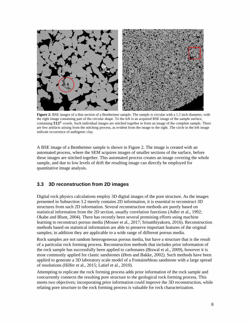
Figure 2: BSE images of a thin section of a Bentheimer sample. The sample is circular with a 1.5 inch diameter, with
the right image containing part of the circular shape. To the left is an acquired BSE image of the sample surface,
containing 𝟓𝟏𝟐𝟐 voxels. Such individual images are stitched together to form an image of the complete sample. There
are few artifacts arising from the stitching process, as evident from the image to the right. The circle in the left image
indicate occurrence of authigenic clay.
A BSE image of a Bentheimer sample is shown in Figure 2. The image is created with an
automated process, where the SEM acquires images of smaller sections of the surface, before
these images are stitched together. This automated process creates an image covering the whole
sample, and due to low levels of drift the resulting image can directly be employed for
quantitative image analysis.
3.3 3D reconstruction from 2D images
Digital rock physics calculations employ 3D digital images of the pore structure. As the images
presented in Subsection 3.2 merely contains 2D information, it is essential to reconstruct 3D
structures from such 2D information. Several reconstruction methods are purely based on
statistical information from the 2D section, usually correlation functions (Adler et al., 1992;
Okabe and Blunt, 2004). There has recently been several promising efforts using machine
learning to reconstruct porous media (Mosser et al., 2017; Srisutthiyakorn, 2016). Reconstruction
methods based on statistical information are able to preserve important features of the original
samples; in addition they are applicable to a wide range of different porous media.
Rock samples are not random heterogeneous porous media, but have a structure that is the result
of a particular rock forming process. Reconstruction methods that includes prior information of
the rock sample has successfully been applied to carbonates (Biswal et al., 2009), however it is
most commonly applied for clastic sandstones (Øren and Bakke, 2002). Such methods have been
applied to generate a 3D laboratory scale model of a Fontainebleau sandstone with a large spread
of resolutions (Hilfer et al., 2015; Latief et al., 2010).
Attempting to replicate the rock forming process adds prior information of the rock sample and
concurrently connects the resulting pore structure to the geological rock forming process. This
meets two objectives; incorporating prior information could improve the 3D reconstruction, while
relating pore structure to the rock forming process is valuable for rock characterization.
9
One process based 3D reconstruction was introduced in (Bakke and Øren, 1997), where three
steps are applied to mimic the natural occurring rock forming process: Grain sedimentation,
compaction and diagenesis. The grain sedimentation is modelled by creating a sphere pack with a
size distribution representative for the grain size distribution. Compaction is modelled by a linear
shift of the grains in the vertical direction. The main elements of the diagenesis modeling are to
simulate quartz overgrowth, clay and cement precipitation. Quartz might be modelled using a
method introduced in (Pilotti, 2000), while clay and cement are usually distributed statistically.
Such a process based modeling technique has been shown to be more predictive than typical
statistical reconstruction techniques (Hilfer and Manwart, 2001).
4 Image analysis
Imaging involves processing to enhance the image quality, e.g. beam hardening correction,
removal of ring artifacts, filtering, etc. (Wildenschild and Sheppard, 2013). Such processing is
essential to obtain high quality images, however it is considered outside the scope of this paper.
In this section we consider image analysis on already processed images.
The input for simulation of transport processes are 3D structures containing few phases, often
simply binary images representing only the matrix and pore space (Iassonov et al., 2009). This
requires processing of the rock sample images irrespectively of where they are originating from;
micro-CT, SEM or other methods. Segmentation into the relevant phases needs to be calibrated,
as the segmentation process is non-unique (Andrä et al., 2013a; Leu et al., 2014; Schembre-
McCabe et al., n.d.). In addition to an input for simulations, image analysis can provide further
information of the samples; e.g. grain- and pore-size distribution, mineralogy, and clay content.
4.1 Mineralogy
Mineralogy is one of the key parameters in characterizing rocks. One commonly applied method
to quantify the mineralogy is X-ray diffraction measurements of crushed samples (Środoń et al.,
2001). This involves crushing the sample to a powder, the method is thus destructive and it gives
no information on spatial relationships. Another commonly applied method is optical
petrography. Samples can be inspected manually, e.g. by point-counting methods (Walderhaug et
al., 2012), or by digital image analysis (Grove and Jerram, 2011).
In both micro-CT and BSE images the gray scales correlates to the density of the material, thus
such gray scale images have information on the mineralogy of the sample. Unfortunately,
different minerals might have similar gray values, e.g. the BSE values for quartz and plagioclase
are similar, hampering mineral identification.
Other methods to obtain more quantitative measurements for mineralogy are available. It is
possible to back-calculate density values from dual-energy scans, i.e. a set of two micro-CT scans
obtained at different energy levels, however this is more widely used on larger scales such as
whole cores (Lopez et al., 2016). For thin sections it is common to apply energy-dispersive X-ray
microanalysis (EDS) in combination with SEM to obtain elemental information (Minnis, 1984).
Together with a mineral identification system this can give high resolution mineral map of the
imaged core sample (Gottlieb et al., 2000; Knackstedt et al., 2010). Mineral quantification can be
used in rock typing directly, by separating different rock types based on the amount of different
minerals.

10
4.2 Porosity classification
Porosity information is obtained from images by segmentation. For a dry sample in ambient
conditions the pore space is filled with air. It is typically straight forward to detect large pore
bodies in micro-CT images, as air has low X-ray attenuation compared to minerals such as quartz.
Smaller pores, e.g. tight pore throats and pores inside clays, is typically not fully resolved in a
micro-CT image. With SEM imaging such pores can be resolved, but higher resolution is
conflicting with the objective of obtaining a REV. Exemplary, authigenic clays has pore sizes in
the range of 100Å to 1000Å, which are several orders of magnitude smaller than grains (Hurst
and Nadeau, 1995). Thus resolving such small pores and at the same time capturing a REV is
hardly possible in 2D, while it is clearly outside present capabilities in 3D.
When excluding fractures, sandstone porosity can be classified into three types: Intergranular,
dissolution and micro (Pittman, 1979). The integranular porosity is the primary porosity between
the grains. Dissolution of soluble rock components, e.g. feldspar grains, creates dissolution
porosity. Completely dissolved components can create large vugs, which gives a larger effect on
porosity than permeability. Microporosity is commonly defined by size, e.g. pores smaller than
0.5𝜇𝑚, and occurs e.g. in clays. There might be significant overlap between these porosity
definitions. When working with images it is common to classify the porosity after how it is
resolved in the image: The resolved porosity is defined as effective porosity, while porosity
below the image resolution is called microporosity (Lopez et al., 2013). The separation between
effective and micro-porosity is thus dependent on the image resolution and image quality.
The capillary pressure is linked to pore sizes through the Young-Laplace equation:
𝑃𝑐 =
2𝜎 cos 𝜃
𝑟,
( 1 )
where 𝜎 is the interfacial tension, 𝜃 is the contact angle, and 𝑟 is the radius of the pore. For
mercury imbibition into a dry core it is common to assume that the contact angle is constant as
mercury is non-wetting for most materials. The interfacial tension is also assumed constant, thus
the capillary pressure is inversely proportional to the pore radius from the Young-Laplace
equation. One can therefore get information of the pore size distribution by monitoring the
capillary pressure during a mercury intrusion experiment (Purcell, 1949). Measurements of high
accuracy can actually observe when single pore throats are intruded by the mercury (Yuan and
Swanson, 1989).
We can quality control the accuracy of the pore structure for a segmented pore space from a
micro-CT image, equivalently the pore space in a reconstructed 3D structure from a 2D image, by
comparing a mercury injection simulation to experimental data. Such a comparison is shown in
Figure 3. Note that the simulated mercury intrusion saturations have been scaled by the fraction
of resolved porosity in the images to the measured porosity on the corresponding plug used in the
mercury experiment. The difference between resolved and measured porosity is then attributed to
pores smaller than the image resolution. The good match between simulated and experimental
data observed in Figure 3 indicates that the image segmentation has captured the pore structure to
a high degree of accuracy. This yields a good starting point for further numerical simulations.

11
Figure 3: Plots of a simulated mercury intrusion for a segmented micro-CT image of a core plug together with
experimental mercury intrusion conducted on a sister plug. Note that for the simulated data we do not have pore throats
smaller than the image voxel size.
It is evident from Figure 3 that a significant fraction of the pore space is not contained in the
resolved porosity in the image. SEM imaging obtains better resolution than micro-CT images.
Still pores bellow the image resolution, e.g. pores inside clays, is common when the image
capture a REV. As clays are porous, their gray scale values are commonly between the values
associated with quartz and porosity, as indicated with a red circle in Figure 2. This enables
segmentation of the microporous phase.
4.2.1 Effective porosity
The Hagen–Poiseuille equation gives the volumetric flow rate 𝑄 through a pipe as
𝑄 =
𝜋𝑟4
8𝜇∇𝑃,
( 2 )
where 𝑟 is the pipe radius, 𝑃 is the pressure, and 𝜇 is the viscosity. As the flow rate is
proportional to the cross-sectional area squared, the smallest pores has little impact on overall
flow. If the image resolution is sufficient to properly resolve the pore space containing the
backbone of the fluid flow, then simulations on the resolved pore space would capture the
important features of the fluid flow. On the other hand, smaller pores give small contribution to
the overall flow, and they are therefore of little importance when trying to capture the main
impacts on the fluid flow in our simulations. They can however be important for saturations and
electrical conductance.
The effective porosity is sometimes defined as the porosity that contributes to fluid flow. As the
smallest pores have little effect on the overall fluid flow, they are commonly excluded from the
effective porosity. If the image resolution is fine enough for simulations to capture the main
portion of the fluid flow, then the resolved porosity corresponds to the effective porosity.
Identifying the resolved porosity with effective porosity is thus dependent on sufficient image
resolution and quality. The amount of resolved porosity in Figure 3 indicates a sufficient image
resolution to capture the main flow paths, as the majority of the pore throats are resolved
properly. Tighter rocks would require a higher resolution. In the following we assume that the

12
image resolution is fine enough to resolve the main flow paths, and would therefore equate
resolved and effective porosity.
As the contribution to flow from the smallest pores might be ignored, it is expected that the
effective porosity has a better correlation with permeability than the total porosity (Nordahl et al.,
2014). In Figure 4 we have plotted both helium and effective porosity versus permeability for a
set of samples from a field at the Norwegian Continental Shelf (NCS). The thin sections have
been produced from end caps of a set of core plugs, and the helium porosity and permeability
values are from the corresponding core plug. More information on the imaging procedure can be
found in (Lopez et al., 2013).
As expected we observe an improved porosity-permeability correlation for the effective porosity
over the helium porosity. On should note that we obtain an improved porosity-permeability
correlation despite the fact that the effective porosity is calculated from a thin section
representing a cross-section at one end of the core sample. Heterogeneities in the sample not
represented at the end-cap cross-section will therefore not be accounted for. Improvements in the
porosity-permeability correlation have been observed for a large variety of reservoirs, and the
strongest improvements occur for fairly homogeneous reservoirs.
Figure 4: Plot comparing the correlation of helium porosity and effective porosity from thin sections versus
permeability.
4.2.2 Microporosity
While the fluid flow rate in a tube is proportional to the cross-sectional area squared, electrical
conductance is proportional to the area. To accurately simulate electrical conductance the
unresolved porosity must be accounted for. For lower permeability samples the unresolved
porosity is important for simulation of fluid flow too.
For both micro-CT and SEM images unresolved porosity typically gives gray levels between
quartz and fully resolved porosity, as observed for the micro-CT image at the left in Figure 6 and
for the BSE image in Figure 2. This enables direct segmentation of the unresolved porosity. Let
𝑉𝑚 be the fraction of pixels with grey levels between the levels associated with quartz and
resolved porosity. Assuming a constant porosity fraction 𝜇𝑚 for the unresolved porosity, then the
amount of porosity associated to the unresolved pores is:

13
𝜙𝑚 =
𝑉𝑚𝜇𝑚
𝑉𝑡,
( 3 )
where 𝑉𝑡 is the total amount of pixels in the image. If 𝜙𝑒 is the effective porosity (resolved
porosity) in the image, then the total porosity is given by the sum
𝜙 = 𝜙𝑒 + 𝜙𝑚. ( 4 )
We can now treat the micro-porosity fraction 𝜇𝑚 as an adjustable variable to minimize the
difference between image porosity and measured porosity. The micro-porosity in samples from
the NCS is mainly associated with clays, mostly kaolinite. Depending on clay types, resolution
and segmentation, the micro-porosity fraction 𝜇𝑚 is typically around 0.5 for BSE images of NCS
samples with resolution around 1 𝜇𝑚. For the samples considered in Figure 4 we used a fraction
of 𝜇𝑚 = 0.4. Calculated image porosity versus helium porosity for the corresponding plugs is
plotted in Figure 5. The clustering around the 1-1 line fraction gives confidence in the
microporosity value of 𝜇𝑚 = 0.4.
Figure 5: Helium porosity versus the calculated image porosity from the corresponding thin sections.
One method to obtain a better porosity image from micro-CT imaging is dry-wet imaging. With
this method the same sample is imaged both in dry state and fully saturated with brine (Bhattad et
al., 2014; Feali et al., 2012; Long et al., 2013). The brine is added a strongly X-ray attenuating
dope to increase the contrast. Example images of dry and wet samples are presented in Figure 6.
Such dry-wet imaging has the advantage that it can reveal sub-resolution pores, i.e.
microporosity. The red circle in Figure 6 indicates voxels with attenuation between that of pores
and quartz. The center image in Figure 6 shows that these voxels still have attenuation values
between pore and quartz when pores have a higher X-ray attenuation than quartz as the sample
has been filled with doped brine. This indicates that these voxels are influenced by the doped
brine, and therefore represents a microporous phase. The difference between the dry and wet
image produce an image of the porosity of the sample. The gray-levels of the difference image
corresponds to the porosity value for the voxel, and can be utilized to estimate the porosity
fraction 𝜇𝑚 for the unresolved porosity.

14
Figure 6: Cross-section of micro-CT image of Bentheimer sample. Left image shows dry sample, centre image shows
sample saturated with dope brine, while right image show sample when drained to irreducible water saturation. The red
circle indicates unresolved porosity.
4.2.3 Irreducible water saturation
When oil (equivalently, gas) imbibes a water-filled rock, it first invade the largest pore-throats
according to the Young-Laplace equation ( 1 ). Oil will enter smaller and smaller pore-throats as
the capillary pressure increase. For a pore-throat size of 0.1𝜇𝑚, assuming an interfacial tension of
𝜎 = 0.03𝑁/𝑚 and a contact angle of 𝜃 = 𝜋/6, the Young-Laplace equation gives a capillary
pressure of 5.2𝐸5 Pa, or approximately 5 bar. To reach such a capillary pressure in a reservoir
with a water oil system of densities 1000 𝑘𝑔/𝑚3 and 800 𝑘𝑔/𝑚3, respectively, we need an oil
column of height ℎ = 5.2𝐸5𝑃𝑎/(200𝑘𝑔/𝑚3 ∗ 9.81𝑚/𝑠2) = 265𝑚, which is considered a high
oil column.
Most capillary pressure experiments are stopped at 5 bar, as capillary pressures experienced in the
reservoir is assumed to be below this value. When plotting water saturation versus capillary
pressure, most sandstones exhibit an asymptote before reaching 5 bar. This asymptote is assumed
to distinguish the effective porosity from the micro-porosity, and oil will not enter the micro-
porosity. The water saturation at this asymptote is interpreted as the irreducible water saturation
𝑆𝑤𝑖𝑟𝑟. As the capillary pressure curves do not always exhibit an asymptote, the irreducible water
saturation is not well defined. It is therefore common to define the irreducible water saturation as
the water saturation at a capillary pressure of 5 bar.
From the calculations above, an irreducible water saturation defined as the saturation at 5 bar
capillary pressure corresponds to a pore-throat size of approximately 0.1 𝜇𝑚. Given the aspect
ratio between pore body and pore throat, this corresponds to porosity not resolved by an image
resolution around 1𝜇𝑚. For such images, we can then estimate the irreducible water saturation
with the formula:
𝑆𝑤𝑖𝑟𝑟 =
𝜙𝑚
𝜙.
( 5 )
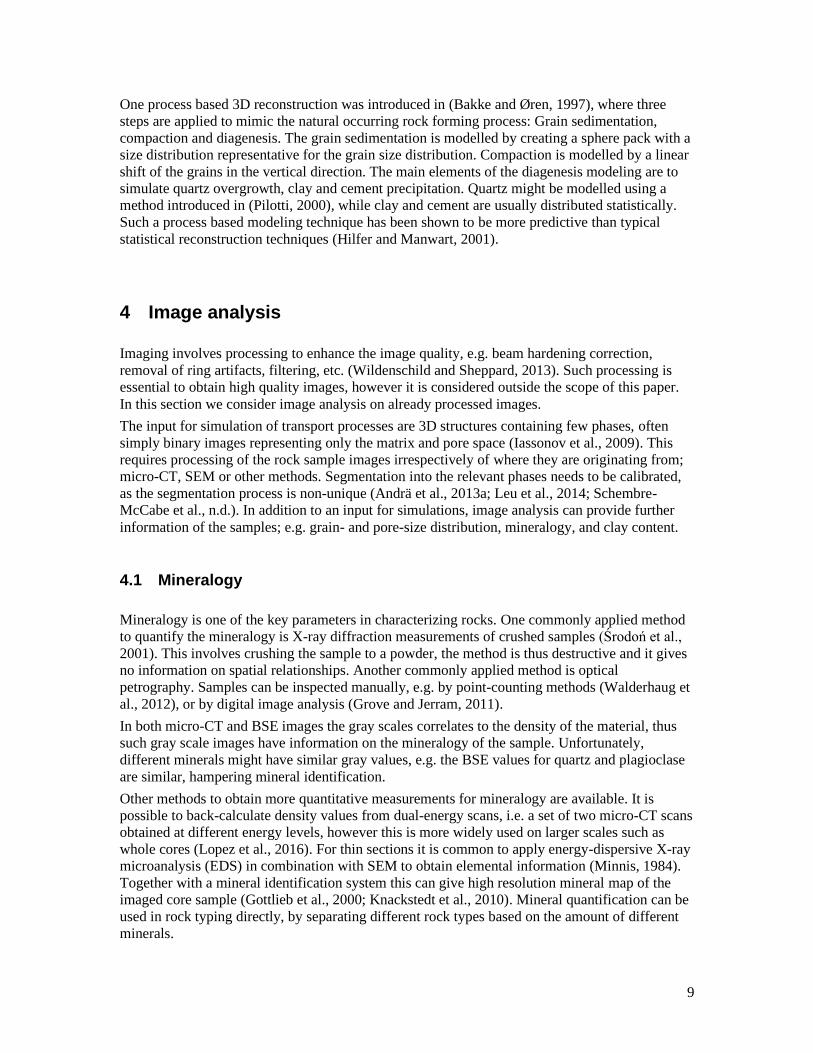
In Figure 7 we have plotted the irreducible water saturation calculated using Equation ( 5 ) versus
permeability. The experiments were conducted using a porous plate method with a maximum end
pressure of 5 bar. We observe that the irreducible water saturation from image analysis gave a
similar trend as the experiments. For this set of core plugs, most of the unresolved porosity was
associated with clays. The negative correlation between irreducible water saturation and
permeability is as expected as the clay fill and blocks pores (Coskun and Wardlaw, 1995; Hamon
and Pellerin, 1997).
15
Figure 7: Permeability versus irreducible water saturation. The plot includes porous plate experimental data and the
calculated values for thin section from the same well.
4.3 Grain size and distribution
The grain size distribution is an integral part of the sedimentological description of reservoir
rocks. While visual and optical microscopy might give reliable grain size data, one can obtain
higher quality data by imaging on the pore scale.
Grain sizes can be extracted directly from a segmented image whenever the image resolves the
individual grains. Codes for extracting the grain size are readily available in visualization
software such as ImageJ and Avizo. Many grain identification routines are sensitive to noise.
Fortunately, the adverse effect from filtering, e.g. a median filter on the segmented binary image,
diminishes when the voxel resolution becomes significantly smaller than the grains.
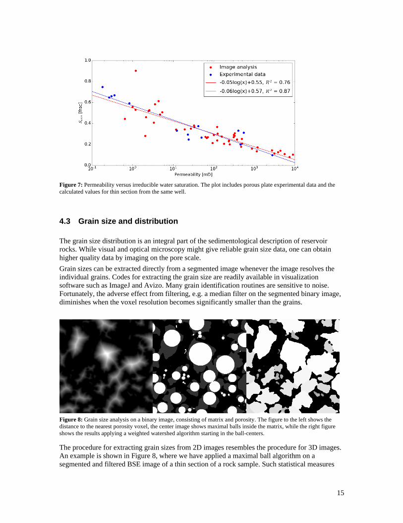
Figure 8: Grain size analysis on a binary image, consisting of matrix and porosity. The figure to the left shows the
distance to the nearest porosity voxel, the center image shows maximal balls inside the matrix, while the right figure
shows the results applying a weighted watershed algorithm starting in the ball-centers.
The procedure for extracting grain sizes from 2D images resembles the procedure for 3D images.
An example is shown in Figure 8, where we have applied a maximal ball algorithm on a
segmented and filtered BSE image of a thin section of a rock sample. Such statistical measures

16
give an estimate for the grain size distribution, and can be used directly if one only compares 2D
distributions. If one need the 3D grain size distribution, e.g. for generating a 3D rock model, the
stereological effect needs to be accounted for.
A BSE image of a thin section can be considered as an infinitesimal plane through the rock
sample. Given a sphere of radius 𝑟, a plane cutting through the sphere at a distance 𝑙 from the
center gives a circle of radius 𝑟′ = √𝑟2 − 𝑙2. This translates into a probability distribution as
plotted in Figure 9. The grain size distribution of a monodispersed grain pack is plotted in the
same figure. As seen from the plots, there is a fair correspondence between the analytical
probability distribution and the disk sizes from the cross-section of the sphere pack.
To back-calculate the original 3D distribution, let us represent the observed size distribution by a
vector �⃗⃗� = (𝑤𝑖), where 𝑤0 corresponds to the smallest grain size bin, while 𝑤𝑛 corresponds to
the largest. Then let 𝑃 = (𝑝𝑖,𝑗) be the 𝑛 × 𝑛 triangular matrix with
𝑝𝑖,𝑗 = 1/𝑗 (√𝑗2 − (𝑖 − 1)2 − √𝑗2 − 𝑖2) ∀𝑖 ≤ 𝑗.
Then ∑ 𝑝𝑖,𝑗𝑗𝑖=0 = 1, and if 𝑣 is the distribution of the 3D sphere radius, then �⃗⃗� = 𝑃𝑣 , thus 𝑣 =
𝑃−�⃗⃗� . To ensure 𝑣 only consists of positive elements one can use an iterative method to minimize ‖�⃗⃗� − 𝑃𝑣 ‖. Note that this estimate gives the size distribution of the spheres represented in the
cross-section. To obtain an estimate of the 3D size distribution one need to adjust for the volume
the spheres occupy.
Figure 9: Probability distribution for a mono-dispersed sphere pack, together with a cross-section of the sphere pack.
The shades of gray in the cross-sectional image correspond to the different disk sizes.
The permeability is described by the pore structure as
𝑘 =
𝜙𝑙𝑐2𝜏2
𝐶,
( 6 )
where 𝑙𝑐 is a characteristic length of the pore space, the tortuosity 𝜏<1 represents the sinuosity of
the flow paths, while the constriction factor 𝐶 represents the aspect ratio between the pore bodies

17
and pore throats (Berg, 2014). The grain size is closely related to the characteristic length 𝑙𝑐, and
thereby to the permeability.
Figure 10: Coarse grained sample from Field 1 of 1.5 inch diameter. Image analysis gave an inter-granular porosity of
20.5%, clay fraction of 7.4%, and volume weighted mean grain size of 474𝝁m. The permeability of the corresponding
core plug was 11.8D.
Figure 11: Fine grained sample from Field 1 of 1.5 inch diameter. Image analysis gave an inter-granular porosity of
21.4%, clay fraction of 10.6%, and volume weighted mean grain size of 100𝝁m. The permeability of the corresponding
core plug was 477mD.
BSE images of two rock samples from a reservoir at the NCS are shown in Figure 10 and Figure
11. We observe that these samples have clearly different grain sizes. However, when
investigating the enlarged section, the grain size distribution and the pore structure has
similarities. As the tortuosity 𝜏 and constriction factor 𝐶 are scale invariant (see (Berg, 2014)),
such similarities indicates similar tortuosity and constriction factor for the two samples. Also the

18
porosity for the two samples are similar. Applying Eq. ( 6 ), where subscript 1 is for the coarse
sample in Figure 10 while subscript 2 is for the fine grained sample in Figure 11, we obtain:
𝑘1
𝑘2=
𝜙1𝑙12𝜏1
2
𝐶1
𝐶2
𝜙2𝑙22𝜏2
2 ≃𝑙12
𝑙22 ~
(474𝜇𝑚)2
(100𝜇𝑚)2= 22.5
This is a fair correspondence with the measured fraction of 𝑘1/𝑘2 = 11800/477 =24.7,
indicating that the grain size is a first order effect for the permeability difference between these
two samples.
Grain sorting impacts both the characteristic length, porosity and constriction factor. In general,
rocks with a large variance in grain size exhibit a short characteristic length, low porosity and
high constriction factor. Large variation in grain size then implies lower permeability from
Equation ( 6 ). In Figure 12 we have plotted the mean and standard deviation of the grain size
distribution in Krumbein 𝜙-scale. The scatter points are colored by the logarithm of the
corresponding permeability divided by porosity. Note that in the Krumbein 𝜙-scale a lower value
indicates a larger grain size. Thus a lower mean grain size value in Figure 12 indicates a larger
grain size. The larger grain size correlates with a higher value for the permeability divided by
porosity, as expected. A lower variance also correlates with higher value for the permeability
divided by porosity. We observe that lower values for both mean and variance in Figure 12
correlates with higher permeability divided by porosity.
Figure 12: Plot of mean and standard deviation of the grain size distribution from a set of thin section data. The plot is
colored by the corresponding logarithm of permeability divided by porosity.
In Figure 12 we have also include 5 pore scale models. These models were generated using a
grain size distribution given by a normal distribution on the Krumbein 𝜙-scale with the indicated
mean and standard deviation. Observe that the permeability divided by porosity for the generated
models are in fair correspondence with the experimental data, indicating the importance of the
grain size distribution on the permeability.

19
5 Simulation
Digital representation of the pore structure enables the simulation of physical processes to obtain
effective porous medium properties. Such effective porous medium properties include absolute
and relative permeability, electrical conductance, diffusion and elasticity. In this section we will
discuss and compare different methods for calculating these effective properties.
5.1 Absolute and relative permeability
Methods to calculate the permeability can be divided into two main groups; modeling directly on
grid representation and network modeling (Blunt et al., 2013). Both methods have its strengths
and weaknesses.
Direct modeling is usually conducted on a binarized image of the pore structure. Such images can
be obtained by the different methods described in Section 3 and 4. Direct modeling thus honors
the geometry in the digitized image. On the other hand they are computational demanding and
have limited possibilities to include effects happening below the voxel size.
As the name suggest, network modeling extracts a network representation of the pore structure
(Fatt, 1956). This honors the underlying topology and overall volumes, however it is a
simplification that does not take all the finer details of the pore geometry into account. The main
benefit of network modeling is computational efficiency and resolution (Valvatne and Blunt,
2004).
As mentioned in the introduction, capillary dominated pore filling processes during primary
drainage has simpler fluid-fluid and fluid-rock interactions. This enables the modeling of these
processes solely based on pore structure information (Hilpert and Miller, 2001). Such pore
structure based simulations has been shown to closely match experimental pore scale data for
primary drainage (Hussain et al., 2014), while imbibition processes need more information for
accurately modeling (S. Berg et al., 2016). Another option for a capillary dominated displacement
is to use the level-set method to track fluid interfaces (Prodanović and Bryant, 2006).
The most popular direct modeling technique is the lattice-Boltzmann method. Historically this
method evolve from the lattice-gas automata models, employing a Boltzmann equation to model
the single-particle lattice gas (McNamara and Zanetti, 1988). The method relies on a simplified
collision and propagation scheme, and can be shown to approximate the Navier-Stokes equation.
The popularity of this method partly arises from the fact that it is easy to implementation and well
suited for parallelization. In addition it can be extended to multiphase flow as fluid-fluid and
fluid-solid interactions are straight forward to include (Ramstad et al., 2012). In particular, phases
can easily be tracked as particles represent fluid elements, while there are several different
methods for fluid separation (Gunstensen et al., 1991; Mcclure et al., 2016; Shan and Chen,
1993). Fluid separation by both the color gradient and the free energy model has been shown to
accurately capture the dynamics of capillary filling events (Ryan T. Armstrong et al., 2016;
Zacharoudiou and Boek, 2016).
For slow flow the Navier-Stokes equation can be simplified to the Stoke equation. For single
phase flow the Stokes equation has been solved by an artificial compressibility method (Bentz
and Martys, 2007; Berg and Held, 2016). Multiphase flow has been treated by solving the Navier-
Stokes equation while tracking the fluid interface, e.g. by a volume-of-fluid technique (Hirt and
Nichols, 1981). Several groups has used the openFOAM framework for such volume-of-fluid
two-phase flow simulations (Ferrari and Lunati, 2013; Raeini et al., 2012).

20
Another direct modeling technique is the Smoothed Particles Hydrodynamics (SPH), where fluid-
fluid surface tension is simulated by interaction forces between different particles (Morris, 2000;
Tartakovsky and Meakin, 2006). In contrast to the Lattice-Boltzmann technique, the SPH
techniques can handle larger viscosity and density contrasts. The SPH technique has recently
been used to model micromodel experiments of multiphase flow (Kunz et al., 2016;
Sivanesapillai et al., 2016).
Direct hydrodynamic (DHD) simulation is a fairly new method based on classical continuum
hydrodynamics. DHD takes into account thermodynamic energy balance in addition to mass and
momentum, while fluid-fluid interaction is modeled with the density functional approach
(Demianov et al., 2011). It has been demonstrated that the method can reproduce a wide range of
basic two-phase flow mechanisms (R. T. Armstrong et al., 2016). Digital rock modeling applying
the DHD method is commercially available (Koroteev et al., 2014).
As mentioned, network modeling involves extracting a network representation of the pore
structure, where larger voids defined as pores are connected by smaller voids defined as throats.
For complex pore structures there are no unique definition of pores and pore throats, thus
different network extraction methods produces different networks (Dong and Blunt, 2009).
Reconstructed porous media, as described in Section 3.3, contains information about the borders
of the individual grains. Invoking grain information benefits the network extraction in the sense
that it reduces the freedom in separating pores and throats (Bakke and Øren, 1997).
The validity of networks could be tested by comparing their transport properties to direct
solutions. Even though direct simulations are computational heavier than network simulations,
simulation of single phase properties such as permeability and electrical conductance are light
enough to be used for quality control of network models. Confidence in the network model is
strengthen when calculated values for permeability and electrical conductance are comparable for
the direct and network model. Also the individual pore structure descriptors for transport given in
Equation ( 6 ) has been applied to validate pore networks (Berg, 2013).
Simulation of multiphase flow in pore networks is typically quasi-static and restricted to a flow
regime dominated by capillary forces (Oren et al., 1998). There exists dynamic simulators that
can account for viscous forces, however these are still at a research state (Nguyen et al., 2006).
The picture is quite opposite for direct modeling; direct modeling takes viscous forces into
account, and simulations get more computational demanding when capillary forces starts to
dominate. With direct simulations one circumvents the inherent issue of creating a representative
network. Unfortunately they are so computational demanding that it is hard to capture a REV and
at the same time resolving film flow. Networks have in practice infinite resolution, and film flow
is incorporated in commercially available simulators.
The pros and cons for direct modeling and network modeling indicate that the method of choice is
highly dependent the objectives for the investigation. Exemplarily, when modeling high flow
rates or low surface tension the viscous forces become dominant, and direct modeling is typically
the method of choice. Conversely, when modeling end-point saturations in a capillary dominated
regime, then film flow is a first order effect and network modeling is typically the method of
choice. The service industry delivering digital rock modeling has been divided between focusing
on direct modeling (Koroteev et al., 2014) and network modeling (Bakke and Øren, 1997).
5.2 Electrical conductance and steady-state diffusion
Both electrical conductance and steady-state diffusion is governed by the Laplace equation, thus
they have equivalent solutions. We will only consider electrical conductance in this paper. From
the Hagen–Poiseuille equation, Equation ( 2 ), we saw that for a tube the fluid flow rate is

21
proportional to the cross-sectional area squared. However, the electrical conductance of an
electrolyte in a tube is correlated with the area. The effective electrical conductance 𝜎𝑐 for a non-
conductive porous medium filled with an electrolyte of conductance 𝜎 is described by the pore
structure as (Berg, 2012):
𝜎𝑐
𝜎=
𝜙𝜏𝑐2
𝐶𝑐.
( 7 )
The equation is analogue to Equation ( 6 ) for permeability, however it does not contain a
characteristic length as the electrical conductance is correlated to the area instead of the area
square. Note that the tortuosity 𝜏𝑐 is an explicit integral of electric field line lengths. As the
electric field lines are different from the fluid streamlines, the electrical tortuosity 𝜏𝑐 is different
from the fluid flow tortuosity 𝜏. Analogous, the electrical constriction factor 𝐶𝑐 differs from the
fluid flow constriction factor 𝐶.
As the electrical conductance correlates with the area, the contribution from the microporosity to
overall conductance is significant. Simulation of electrical conductance therefore needs to
account for the microporosity. If the microporous phase is assumed homogeneous, then one could
calculate its effective electrical conductance on high resolution FIB-SEM images or reconstructed
3D structures from high resolution SEM images of the microporous phase. Such procedures has
been conducted for micrite in carbonates and clays in sandstones (Lopez et al., 2012; Ruspini et
al., 2016). Without such micro-pore models one could use trend analysis to obtain a relation for
the tortuosity and constriction factor versus porosity for the microporous phase (Rezaei-Gomari et
al., 2011).
With a 3D model of the pore structure, including effective conductance for the microporous
phase, the Laplace equation can be solved using e.g. a conjugate gradient method. The surface
conductance can also be included into such calculations (Johnson et al., 1986); however the
surface conductance is typically of second order for reservoir salinities. The resulting electric
field then gives an effective porous medium conductance 𝜎𝑐 for a given electrolyte conductance
𝜎, which yields the formation factor 𝐹 = 𝜎/𝜎𝑐. For a multiphase flow simulation one might
compute the electrical conductance for the water phase for each saturation step, which yields the
resistivity index.
5.3 Elastic properties
There exists a range of methods for obtaining different elastic properties (Andrä et al., 2013b).
Assuming a linear elastic regime, the local equations governing the static elastic behavior can be
solved by finite element methods (Garboczi and Day, 1995). Such methods has been applied to
grid models of sandstones (Øren et al., 2007). In highly consolidated materials the grain-grain
connections are properly resolved. For such consolidated material, e.g. Fountainebleau samples,
computed elastic properties is in fair agreement with experimental data (Arns et al., 2002). For
less consolidated materials, e.g. sand packs, grain-grain interfaces are not properly resolved. Thus
calculation of elastic properties tends to have the same issues with scale and resolution as for
fluid flow and electrical properties. Unfortunately, robust workarounds for reservoir sandstones
are still not on an industrial standard, thus calculation of elastic properties has not had a wide
adoption yet. We will therefore not consider elastic properties in the remainder of this paper.
6 Application example
22
This section describes an example of industrial application of digital rock technology. We will
consider a field on the NCS together with a smaller satellite field. The main aim of this digital
rock application was to provide flow parameters for the satellite field within a short time frame.
Depending on results from the rock characterization, a secondary aim was to apply the generated
flow parameters for the main field.
Based on results in (Lopez et al., 2010), we consider the digital rock modeling presented in this
section reliable for samples with resolved porosity larger than 10%, permeability larger than
10mD and clay content below 15%. While no objective quantification of grain size distribution
could cover all eventualities, in our experience the radius ratio between the smallest and largest
grains should not be much larger than 1:10 for models to properly resolve both the smallest and
largest grains. This operational range is for model sizes around 1000^3 voxels. Larger models or
other modeling techniques can extend the operational range.
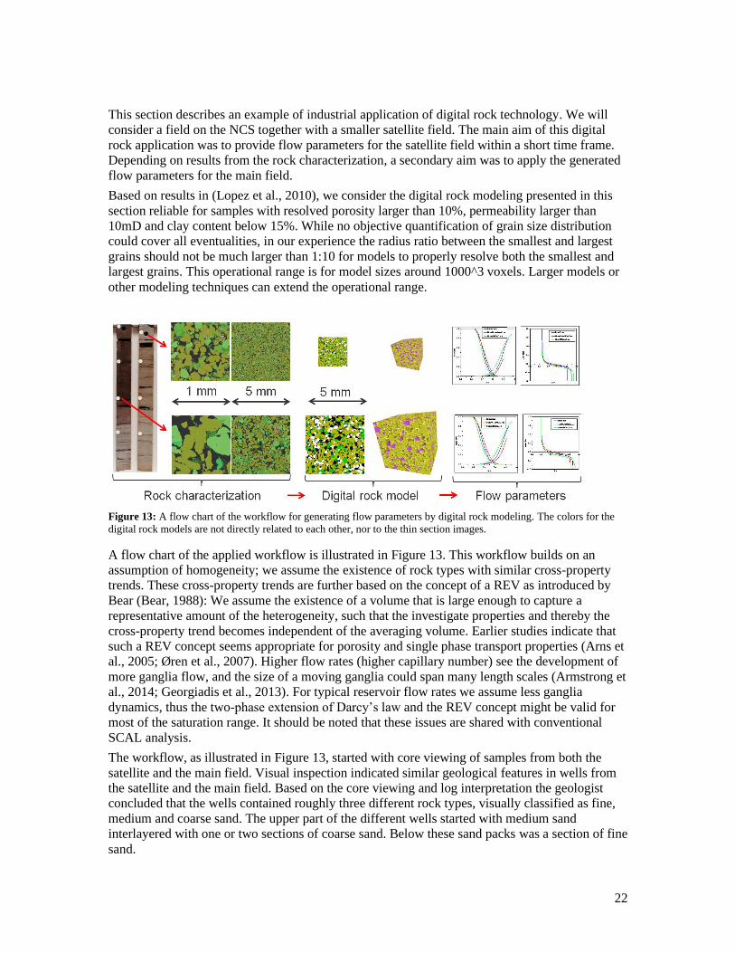
Figure 13: A flow chart of the workflow for generating flow parameters by digital rock modeling. The colors for the
digital rock models are not directly related to each other, nor to the thin section images.
A flow chart of the applied workflow is illustrated in Figure 13. This workflow builds on an
assumption of homogeneity; we assume the existence of rock types with similar cross-property
trends. These cross-property trends are further based on the concept of a REV as introduced by
Bear (Bear, 1988): We assume the existence of a volume that is large enough to capture a
representative amount of the heterogeneity, such that the investigate properties and thereby the
cross-property trend becomes independent of the averaging volume. Earlier studies indicate that
such a REV concept seems appropriate for porosity and single phase transport properties (Arns et
al., 2005; Øren et al., 2007). Higher flow rates (higher capillary number) see the development of
more ganglia flow, and the size of a moving ganglia could span many length scales (Armstrong et
al., 2014; Georgiadis et al., 2013). For typical reservoir flow rates we assume less ganglia
dynamics, thus the two-phase extension of Darcy’s law and the REV concept might be valid for
most of the saturation range. It should be noted that these issues are shared with conventional
SCAL analysis.
The workflow, as illustrated in Figure 13, started with core viewing of samples from both the
satellite and the main field. Visual inspection indicated similar geological features in wells from
the satellite and the main field. Based on the core viewing and log interpretation the geologist
concluded that the wells contained roughly three different rock types, visually classified as fine,
medium and coarse sand. The upper part of the different wells started with medium sand
interlayered with one or two sections of coarse sand. Below these sand packs was a section of fine
sand.

23
All three rock types consisted of homogeneous sand. As these sands were resolved in the
corresponding reservoir models, it was concluded that there was no need for upscaling of flow
parameters. Less homogeneous sands would have implied one or several upscaling steps to obtain
flow parameters for the appropriate scale (Bhattad et al., 2014; Odsæter et al., 2015; Rustad et al.,
2008).
A set of thin sections were chosen to cover the internal spread in properties for the three rock
types. Both BSE and EDS images of the thin sections were obtained, with examples shown in
Figure 10 and Figure 11. The grain size distributions were extracted as described in subsection
4.3. Resulting grain size distributions are plotted in Figure 14. The naming for the three sand
classes are not necessarily in accordance with the Wentworth size terms, the naming is still kept
for simplicity.
Figure 14: Grain size distribution for samples from the satellite and main field. The colors correspond to the associated
rock type determined during the core viewing.
The SEM images indicated that most microporosity was associated with clay. Image analysis
gave slightly lower amounts of clays for the coarse sand compared to the medium sand. The fine
sand had a large variation in clay amount which correlated with depth. The upper samples, close
to the coarse and medium sand, had clay levels comparable to the coarse and medium samples,
while deeper samples contained significantly more clay.
The differences in grain size and clay amount translate into different trends for permeability
versus porosity, as seen in Figure 15. The coarse and medium samples has higher permeability
values for comparable porosity values, and the larger spread in clay amount for the fine scale
samples translates into a large spread in both permeability and porosity.

24
Figure 15: Porosity versus permeability for different sands, comparing models to experimental data.
Four digital rock models were created to represent the three different sand types, with an extra
model to capture the spread in clay values for the fine grained rock type. Each of these rock
models were generated based on statistics from a single thin section. The porosity, grain size
distribution and mineralogy values for the four corresponding thin sections were all close to the
average for the rock type. Thus the generated digital rock model was assumed to represent the
rock type in general, and not just the single thin section from which it was generated. The digital
rock models are also included in Figure 15, and we observe that they are all aligned with the
permeability trend for the corresponding experimental values for the associated rock type. This is
a further confirmation that the digital rock models are representative for their corresponding rock
types.
Network representations were extracted from the digital rock models. Fluid-fluid and fluid-rock
information for two-phase oil-water simulations was estimated based on experimental data from
the main field. This included an estimated value for interfacial tension value and an estimate of
the wettability of the samples.

25
Figure 16: In blue are saturations calculated using a single set of Archie parameters and irreducible water saturation
value. Computer-processed interpretation (CPI) from well log data is plotted in red. The horizontal gray lines indicate
cell boundaries in the corresponding reservoir model, with height in the order of 1.5 meters.
Capillary pressure curves from the digital rock modeling was assigned to facies in a geo-model of
the main field. Together with depths for fluid contacts, these capillary pressure curves was used
to estimate water saturation in the model. The obtained water-saturation logs are plotted with blue
log curves in Figure 16. The same plot includes computer-processed interpretation (CPI) from
well log data, displayed with red log curves. There is a clear correlation between the two
independent methods, which strengthens the representativeness of the digital rock models even
further.

26
Figure 17: Water-cut for a single producer at the main field. This plot contains both historical data and simulation
results. The historical data is indicated with black dots, while results from flow simulations are indicated using lines.
The blue line is simulations using multiphase flow parameters from digital rock modeling, the green line is simulations
using SCAL data, while the red curve shows a simulation using both sets of data.
The resulting two-phase flow parameters were implemented into the dynamic reservoir model for
the main field. Given the good results for the water saturation model described above, the digital
rock models were assigned to facies in the same way as for the water saturation modeling. The
reservoir model with multiphase data from digital rock modeling produced a fair match with
historical data, as seen for an exemplary production well in Figure 17. We observe that the
simulations based on digital rock modeling results in an earlier water break-through than the
historical data. Except for the water-breakthrough, and given that the simulation model has not
been history matched, the simulation results are in fair agreement with the historical data.
It took less than two months from the first core viewing to delivery of digital rock modeling data.
These data was then obtained significantly faster than conventional experimental data. They were
indeed delivered fast enough to be included in simulations for decisions on field development for
the satellite field.

27
Figure 18: Relative permeability curves from digital rock modeling (blue lines) compared to a set of experimental data.
The experiments were conducted on sister plugs. For all curves the irreducible water saturation is scaled out for
comparison reasons.
When traditional experimental data was obtained at a later stage, the data was compared to the
results from digital rock modeling. Comparisons for one sample is included in Figure 18. This
comparison shows clear differences for the oil relative permeability curve at low water
saturations. There are also significant differences for the endpoints, with the steady-state and
unsteady state flooding experiments indicating higher residual oil values than the digital rock
modeling, while the centrifuge indicates a slightly lower value. The water curves seems to follow
similar trends toward the residual oil endpoint. Given the spread between different experimental
methods, there is a fair agreement between digital rock models and experimental data overall.
The SCAL data was implemented into the reservoir model considered above. This produced a
significantly better result for the water break-through, and arguably better results for the
remainder of the production curve, as shown in Figure 17. It was observed that the main
difference between the digital rock data and the SCAL data was that the digital rock data lacked a
representative curve for the lowest permeability saturation region. We therefore tried to augment
the digital rock data with a single SCAL relative permeability curve for the low permeability
saturation region. The simulation result is denoted combined data in Figure 17. We observe that
the combined data gave an improved match over the SCAL data.
7 Summary
In this paper we have presented an overview of digital rock technology from an industrial
perspective. We have provided examples of industrial employment of digital rock technology,
and also pointed to the adoption of such technology.
While imaging is a starting point for digital rock simulations, it is also a means in itself. Images
of rock samples have direct application in formation evaluation, rock typing and estimation of
irreducible water saturation, as demonstrated in this paper.
As with imaging, also rock modeling is a means in itself. In contrast with both 3D imaging and
traditional experiments, rock modeling gives the ability to do sensitivity studies by constructing
3D models where only one property is changed. This was exemplified by creating rock models
with different grain size distribution, which revealed correspondence between grain size
distribution and permeability. Investigations of the individual effects of changing porosity, clay
amount, degree of cementation, etc. could be performed similarly.

28
It is fairly straightforward to simulate the fluid permeability given a 3D image with sufficient
resolution to resolve the backbone of the fluid flow and at the same time large enough to capture
a REV. For two-phase flow properties the situation is more complex. Network modeling has the
advantage of practically infinite resolution and computational efficiency. As films are resolved in
network models, they might be more reliable for obtaining the residual oil saturation. On the
other hand, simulations directly on the grid remove the inherent uncertainty in network
extraction. Including viscous forces is more straightforward for direct gird simulations than in
network simulations, therefore direct grid simulations are typically the preferred tool for
simulation of enhanced recovery processes.
Industrial applications were exemplified by an application to a field at the NCS. The direct
relation between simulation and imaging offers a robust link between rock types and flow
parameters. The imaging part of digital rock technology contributes to the rock typing, at the
same time simulation provides petrophysical and flow parameters directly related to the images
and thereby the rock types. This helps bridge the gap between geological interpretation,
petrophysics and reservoir simulations.
In the digital rock study described in this paper, flow parameters from digital rock technology
was obtained in a timeframe of 2 month, which was a fraction of the time used for traditional
SCAL. This exemplifies how digital rock technology can be a tool for fast track decisions. The
study also shows how digital rock technology can extend traditional experiments, as traditional
experiments and digital rock technology provides mutual benefits. Imaging and modeling links
geological interpretation and transport properties, and demonstrates how traditional experiments
benefits from digital rock technology. Another example is the possibility to do sensitivity studies.
On the other hand, fast experiments such as mercury injection are important for calibration of
digital rock models.
Digital rock imaging, modeling and simulation have had a large present in academia for decades.
In the last decade it has moved from a fringe activity to a mature technology for the oil industry.
Most large oil companies now have in-house tools and development efforts, while smaller
companies are more dependent on a number of service providers who deliver digital rock
technology.
8 Acknowledgment
We thank Statoil for permission to publish this work.
9 Bibliography
Aarnes, J.E., Kippe, V., Lie, K.-A., Rustad, A.B., 2007. Modelling of multiscale
structures in flow simulations for petroleum reservoirs, in: Geometric Modelling,
Numerical Simulation, and Optimization. Springer, pp. 307–360.
Adler, P.M., Jacquin, C.G., Thovert, J.-F., 1992. The formation factor of reconstructed
porous media. Water Resour. Res. 28, 1571–1576.

29
Al-Raoush, R., Papadopoulos, A., 2010. Representative elementary volume analysis of
porous media using X-ray computed tomography. Powder Technol. 200, 69–77.
https://doi.org/10.1016/j.powtec.2010.02.011
Andersen, M., Duncan, B., McLin, R., 2013. Core truth in formation evaluation. Oilfield
Rev. 25, 16–25.
Andrä, H., Combaret, N., Dvorkin, J., Glatt, E., Han, J., Kabel, M., Keehm, Y., Krzikalla,
F., Lee, M., Madonna, C., 2013a. Digital rock physics benchmarks—Part I:
Imaging and segmentation. Comput. Geosci. 50, 25–32.
Andrä, H., Combaret, N., Dvorkin, J., Glatt, E., Han, J., Kabel, M., Keehm, Y., Krzikalla,
F., Lee, M., Madonna, C., 2013b. Digital rock physics benchmarks—Part II:
Computing effective properties. Comput. Geosci. 50, 33–43.
Andrew, M., Bijeljic, B., Blunt, M.J., 2014. Pore-by-pore capillary pressure
measurements using X-ray microtomography at reservoir conditions: Curvature,
snap-off, and remobilization of residual CO2. Water Resour. Res. 50, 8760–8774.
Archie, G.E., 1942. The electrical resistivity log as an aid in determining some reservoir
characteristics. Trans. AIME 146, 54–62.
Armstrong, R. T., Berg, S., Dinariev, O., Evseev, N., Klemin, D., Koroteev, D., Safonov,
S., 2016. Modeling of Pore-Scale Two-Phase Phenomena Using Density
Functional Hydrodynamics. Transp. Porous Media 112, 577–607.
Armstrong, R.T., Georgiadis, A., Ott, H., Klemin, D., Berg, S., 2014. Critical capillary
number: Desaturation studied with fast X-ray computed microtomography.
Geophys. Res. Lett. 41, 55–60.
Armstrong, Ryan T., McClure, J.E., Berrill, M.A., Rücker, M., Schlüter, S., Berg, S.,
2016. Beyond Darcy’s law: The role of phase topology and ganglion dynamics for
two-fluid flow. Phys. Rev. E 94, 043113.
Arns, C.H., Knackstedt, M.A., Martys, N.S., 2005. Cross-property correlations and
permeability estimation in sandstone. Phys. Rev. E 72, 046304.
https://doi.org/10.1103/PhysRevE.72.046304
Arns, C.H., Knackstedt, M.A., Pinczewski, W.V., 2001. Accurate estimation of transport
properties from microtomographic images. Geophys. Res. Lett. 28, 3361–3364.
Arns, C.H., Knackstedt, M.A., Pinczewski, W.V., Garboczi, E.J., 2002. Computation of
linear elastic properties from microtomographic images: Methodology and
agreement between theory and experiment. Geophysics 67, 1396–1405.
Bakke, S., Øren, P.-E., 1997. 3-D pore-scale modelling of sandstones and flow
simulations in the pore networks. Spe J. 2, 136–149.
Bear, J., 1988. Dynamics of fluids in porous media. Dover.
Bekri, S., Howard, J., Muller, J., Adler, P.M., 2003. Electrical Resistivity Index in
Multiphase Flow through Porous Media. Transp. Porous Media 51, 41–65.
https://doi.org/10.1023/A:1021229106005
Bentz, D.P., Martys, N.S., 2007. A stokes permeability solver for three-dimensional
porous media. US Department of Commerce, Technology Administration,
National Institute of Standards and Technology.
Berg, C.F., 2014. Permeability description by characteristic length, tortuosity,
constriction and porosity. Transp. Porous Media 103, 381–400.
Berg, C.F., 2013. A Microstructure Description of the Relationship between Formation
Resistivity Factor and Porosity.

30
Berg, C.F., 2012. Re-examining Archie’s law: Conductance description by tortuosity and
constriction. Phys. Rev. E 86, 046314.
Berg, C.F., Held, R., 2016. Fundamental Transport Property Relations in Porous Media
Incorporating Detailed Pore Structure Description. Transp. Porous Media 112,
467–487.
Berg, C.F., Herrick, D., Kennedy, D., 2016. Geometrical Factor of Conductivity in
Rocks: Bringing New Rigor to a Mature Model, in: SPWLA 57th Annual
Logging Symposium. Society of Petrophysicists and Well-Log Analysts.
Berg, S., Ott, H., Klapp, S.A., Schwing, A., Neiteler, R., Brussee, N., Makurat, A., Leu,
L., Enzmann, F., Schwarz, J.-O., 2013. Real-time 3D imaging of Haines jumps in
porous media flow. Proc. Natl. Acad. Sci. 110, 3755–3759.
Berg, S., Rücker, M., Ott, H., Georgiadis, A., van der Linde, H., Enzmann, F., Kersten,
M., Armstrong, R.T., de With, S., Becker, J., 2016. Connected pathway relative
permeability from pore-scale imaging of imbibition. Adv. Water Resour. 90, 24–
35.
Bhattad, P., Young, B., Berg, C.F., Rustad, A.B., Lopez, O., 2014. X-ray Micro-CT
Assisted Drainage Rock Typing for Characterization of Flow Behaviour of
Laminated Sandstone Reservoirs.
Biswal, B., Øren, P.-E., Held, R.J., Bakke, S., Hilfer, R., 2009. Modeling of multiscale
porous media. Image Anal. Stereol. 28, 23–34.
Blunt, M.J., 1998. Physically-based network modeling of multiphase flow in
intermediate-wet porous media. J. Pet. Sci. Eng. 20, 117–125.
Blunt, M.J., Bijeljic, B., Dong, H., Gharbi, O., Iglauer, S., Mostaghimi, P., Paluszny, A.,
Pentland, C., 2013. Pore-scale imaging and modelling. Adv. Water Resour. 51,
197–216.
Bultreys, T., Boone, M.A., Boone, M.N., De Schryver, T., Masschaele, B., Van
Hoorebeke, L., Cnudde, V., 2015. Fast laboratory-based micro-computed
tomography for pore-scale research: illustrative experiments and perspectives on
the future. Adv. Water Resour.
Carman, P.C., 1937. Fluid flow through granular beds. Trans.-Inst. Chem. Eng. 15, 150–
166.
Coskun, S.B., Wardlaw, N.C., 1995. Influences of pore geometry, porosity and
permeability on initial water saturation—An empirical method for estimating
initial water saturation by image analysis. J. Pet. Sci. Eng. 12, 295–308.
Cromwell, V., Kortum, D.J., Bradley, D.J., 1984. The use of a medical computer
tomography (CT) system to observe multiphase flow in porous media, in: SPE
Annual Technical Conference and Exhibition. Society of Petroleum Engineers.
Curtis, M.E., Ambrose, R.J., Sondergeld, C.H., 2010. Structural Characterization of Gas
Shales on the Micro- and Nano-Scales. Society of Petroleum Engineers.
https://doi.org/10.2118/137693-MS
Demianov, A., Dinariev, O., Evseev, N., 2011. Density functional modelling in
multiphase compositional hydrodynamics. Can. J. Chem. Eng. 89, 206–226.
Dilks, A., Graham, S.C., 1985. Quantitative mineralogical characterization of sandstones
by back-scattered electron image analysis. J. Sediment. Res. 55.
Dong, H., Blunt, M.J., 2009. Pore-network extraction from micro-computerized-
tomography images. Phys. Rev. E 80, 036307.

31
Fatt, I., 1956. The network model of porous media.
Feali, M., Pinczewski, W., Cinar, Y., Arns, C.H., Arns, J.-Y., Francois, N., Turner, M.L.,
Senden, T., Knackstedt, M.A., 2012. Qualitative and quantitative analyses of the
three-phase distribution of oil, water, and gas in bentheimer sandstone by use of
micro-CT imaging. SPE Reserv. Eval. Eng. 15, 706–711.
Ferrari, A., Lunati, I., 2013. Direct numerical simulations of interface dynamics to link
capillary pressure and total surface energy. Adv. Water Resour. 57, 19–31.
Flannery, B.P., Deckman, H.W., Roberge, W.G., D’AMICO, K.L., 1987. Three-
dimensional X-ray microtomography. Science 237, 1439–1444.
Fredrich, J.T., Lakshtanov, D.L., Lane, N.M., Liu, E.B., Natarajan, C.S., Ni, D.M., Toms,
J.J., 2014. Digital Rocks: Developing An Emerging Technology Through To A
Proven Capability Deployed In The Business. Society of Petroleum Engineers.
https://doi.org/10.2118/170752-MS
Garboczi, E.J., Day, A.R., 1995. An algorithm for computing the effective linear elastic
properties of heterogeneous materials: three-dimensional results for composites
with equal phase Poisson ratios. J. Mech. Phys. Solids 43, 1349–1362.
Georgiadis, A., Berg, S., Makurat, A., Maitland, G., Ott, H., 2013. Pore-scale micro-
computed-tomography imaging: Nonwetting-phase cluster-size distribution
during drainage and imbibition. Phys. Rev. E 88, 033002.
Gilliland, R.E., Coles, M.E., 1990. Use of CT scanning in the investigation of damage to
unconsolidated cores, in: SPE Formation Damage Control Symposium. Society of
Petroleum Engineers.
Gomari, K.A.R., Berg, C.F., Mock, A., Øren, P. al-Eric, Petersen Jr, E., Rustad, A.,
Lopez, O., 2011. Electrical and petrophysical properties of siliciclastic reservoir
rocks from pore-scale modeling, in: SCA2011-20 Presented at the 2011 SCA
International Symposium, Austin, Texas.
Gottlieb, P., Wilkie, G., Sutherland, D., Ho-Tun, E., Suthers, S., Perera, K., Jenkins, B.,
Spencer, S., Butcher, A., Rayner, J., 2000. Using quantitative electron microscopy
for process mineralogy applications. JoM 52, 24–25.
Grader, A., Kalam, M., Toelke, J., Mu, Y., Derzhi, N., Baldwin, C., Stenger, B., 2010. A
comparative study of digital rock physics and laboratory SCAL evaluations of
carbonate cores. SCA2010-24 Novia Scotia.
Grove, C., Jerram, D.A., 2011. jPOR: An ImageJ macro to quantify total optical porosity
from blue-stained thin sections. Comput. Geosci. 37, 1850–1859.
Gunstensen, A.K., Rothman, D.H., Zaleski, S., Zanetti, G., 1991. Lattice Boltzmann
model of immiscible fluids. Phys. Rev. A 43, 4320.
Hamon, G., Pellerin, F.M., 1997. Evidencing capillary pressure and relative permeability
trends for reservoir simulation, in: SPE Annual Technical Conference and
Exhibition. Society of Petroleum Engineers.
Hilfer, R., Manwart, C., 2001. Permeability and conductivity for reconstruction models of
porous media. Phys. Rev. E 64, 021304.
Hilfer, R., Zauner, T., Lemmer, A., Biswal, B., 2015. Threedimensional microstructures
at submicron resolution.
Hilpert, M., Miller, C.T., 2001. Pore-morphology-based simulation of drainage in totally
wetting porous media. Adv. Water Resour. 24, 243–255.

32
Hirt, C.W., Nichols, B.D., 1981. Volume of fluid (VOF) method for the dynamics of free
boundaries. J. Comput. Phys. 39, 201–225.
Honarpour, M.M., Cromwell, V., Hatton, D., Satchwell, R., 1985. Reservoir rock
descriptions using computed tomography (CT), in: SPE Annual Technical
Conference and Exhibition. Society of Petroleum Engineers.
Hove, A.O., Ringen, J.K., Read, P.A., 1987. Visualization of laboratory corefloods with
the aid of computerized tomography of X-rays. SPE Reserv. Eng. 2, 148–154.
Hurst, A., Nadeau, P.H., 1995. Clay microporosity in reservoir sandstones: an application
of quantitative electron microscopy in petrophysical evaluation. AAPG Bull. 79,
563–573.
Hussain, F., Pinczewski, W.V., Cinar, Y., Arns, J.-Y., Arns, C.H., Turner, M.L., 2014.
Computation of relative permeability from imaged fluid distributions at the pore
scale. Transp. Porous Media 104, 91–107.
Iassonov, P., Gebrenegus, T., Tuller, M., 2009. Segmentation of X-ray computed
tomography images of porous materials: A crucial step for characterization and
quantitative analysis of pore structures. Water Resour. Res. 45.
Johnson, D.L., Koplik, J., Schwartz, L.M., 1986. New pore-size parameter characterizing
transport in porous media. Phys. Rev. Lett. 57, 2564.
Kalam, Z., Seraj, S., Bhatti, Z., Mock, A., Oren, P.E., Ravlo, V., Lopez, O., 2012.
Relative permeability assessment in a giant carbonate reservoir using Digital
Rock Physics, in: SCA2012-03, International Symposium, Aberdeen, United
Kingdom.
Kelly, S., El-Sobky, H., Torres-Verdín, C., Balhoff, M.T., 2016. Assessing the utility of
FIB-SEM images for shale digital rock physics. Adv. Water Resour. 95, 302–316.
Knackstedt, M.A., Jaime, P., Butcher, A., Botha, P., Middleton, J., Sok, R., 2010.
Integrating Reservoir Characterization: 3D Dynamic, Petrophysical and
Geological Description of Reservoir Facies. Society of Petroleum Engineers.
https://doi.org/10.2118/133981-MS
Koroteev, D., Dinariev, O., Evseev, N., Klemin, D., Nadeev, A., Safonov, S., Gurpinar,
O., Berg, S., van Kruijsdijk, C., Armstrong, R., Myers, M.T., Hathon, L., de Jong,
H., 2014. Direct Hydrodynamic Simulation of Multiphase Flow in Porous Rock.
Petrophysics 55, 294–303.
Kozeny, J., 1927. Über kapillare Leitung des Wassers im Boden:(Aufstieg, Versickerung
und Anwendung auf die Bewässerung). Hölder-Pichler-Tempsky.
Kunz, P., Zarikos, I.M., Karadimitriou, N.K., Huber, M., Nieken, U., Hassanizadeh,
S.M., 2016. Study of multi-phase flow in porous media: comparison of sph
simulations with micro-model experiments. Transp. Porous Media 114, 581–600.
Latief, F.D.E., Biswal, B., Fauzi, U., Hilfer, R., 2010. Continuum reconstruction of the
pore scale microstructure for Fontainebleau sandstone. Phys. Stat. Mech. Its Appl.
389, 1607–1618.
Lemmens, H., Butcher, A., Botha, P.W., 2010. FIB/SEM and Automated Mineralogy for
Core and Cuttings Analysis. Society of Petroleum Engineers.
https://doi.org/10.2118/136327-MS
Leu, L., Berg, S., Enzmann, F., Armstrong, R.T., Kersten, M., 2014. Fast X-ray micro-
tomography of multiphase flow in berea sandstone: A sensitivity study on image
processing. Transp. Porous Media 105, 451–469.
33
Liu, Z., Herring, A., Arns, C., Berg, S., Armstrong, R.T., 2017. Pore-Scale
Characterization of Two-Phase Flow Using Integral Geometry. Transp. Porous
Media 1–19.
Lohne, A., Virnovsky, G.A., Durlofsky, L.J., 2006. Two-stage upscaling of two-phase
flow: from core to simulation scale. SPE J. 11, 304–316.
Long, H., Nardi, C., Idowu, N., Carnerup, A., Øren, P.E., Knackstedt, M., Varslot, T.,
Sok, R.M., Lithicon, A., 2013. Multi-scale imaging and modeling workflow to
capture and characterize microporosity in sandstone, in: International Symposium
of the Society of Core Analysts, Napa Valley, California, USA.
Lopez, O., Berg, C.F., Bakke, S., Boassen, T., Rustad, A.B., 2013. Thin Section Image
Analysis for Estimation of Initial Water Saturation in Siliciclastic Reservoir
Rocks.
Lopez, O., Berg, C.F., Rennan, L., Digranes, G., Forest, T., Krisoffersen, A., Bøklepp,
B.R., 2016. Quick Core Assessment from CT Imaging: From Petrophysical
Properties to Log Evaluation. Int. Symp. Soc. Core Anal. Snowmass Colo. USA.
Lopez, O., Mock, A., Øren, P.E., Long, H., Kalam, Z., Vahrenkamp, V., Gibrata, M.,
Seraj, S., Chacko, S., Al Hammadi, M., 2012. Validation of fundamental
carbonate reservoir core properties using digital rock physics. SCA Aberd. Scotl.
Lopez, O., Mock, A., Skretting, J., Petersen Jr, E.B., Øren, P.-E., Rustad, A.B., 2010.
Investigation into the reliability of predictive pore-scale modeling for siliciclastic
reservoir rocks, in: SCA2010-41 Presented at the 2010 SCA International
Symposium, Halifax, Canada.
Mcclure, J.E., Berrill, M.A., Gray, W.G., Miller, C.T., 2016. Tracking interface and
common curve dynamics for two-fluid flow in porous media. J. Fluid Mech. 796,
211–232.
McNamara, G.R., Zanetti, G., 1988. Use of the Boltzmann equation to simulate lattice-
gas automata. Phys. Rev. Lett. 61, 2332.
McPhee, C., Reed, J., Zubizarreta, I., 2015. Core Analysis: A Best Practice Guide.
Elsevier.
Minnis, M.M., 1984. An automatic point-counting method for mineralogical assessment.
AAPG Bull. 68, 744–752.
Morris, J.P., 2000. Simulating surface tension with smoothed particle hydrodynamics.
Int. J. Numer. Methods Fluids 33, 333–353.
Mosser, L., Dubrule, O., Blunt, M.J., 2017. Reconstruction of three-dimensional porous
media using generative adversarial neural networks. ArXiv Prepr.
ArXiv170403225.
Nguyen, V.H., Sheppard, A.P., Knackstedt, M.A., Val Pinczewski, W., 2006. The effect
of displacement rate on imbibition relative permeability and residual saturation. J.
Pet. Sci. Eng., Reservoir Wettability8th International Symposium on Reservoir
Wettability 52, 54–70. https://doi.org/10.1016/j.petrol.2006.03.020
Nordahl, K., Messina, C., Berland, H., Rustad, A.B., Rimstad, E., 2014. Impact of
multiscale modelling on predicted porosity and permeability distributions in the
fluvial deposits of the Upper Lunde Member (Snorre Field, Norwegian
Continental Shelf). Geol. Soc. Lond. Spec. Publ. 387, 85–109.

34
Nordahl, K., Ringrose, P.S., 2008. Identifying the representative elementary volume for
permeability in heterolithic deposits using numerical rock models. Math. Geosci.
40, 753–771.
Odsæter, L.H., Berg, C.F., Rustad, A.B., 2015. Rate Dependency in Steady-State
Upscaling. Transp. Porous Media 110, 565–589.
Oh, W., Lindquist, B., 1999. Image thresholding by indicator kriging. IEEE Trans.
Pattern Anal. Mach. Intell. 21, 590–602.
Okabe, H., Blunt, M.J., 2004. Prediction of permeability for porous media reconstructed
using multiple-point statistics. Phys. Rev. E 70, 066135.
Øren, P.-E., Bakke, S., 2002. Process based reconstruction of sandstones and prediction
of transport properties. Transp. Porous Media 46, 311–343.
Øren, P.-E., Bakke, S., Arntzen, O.J., 1998. Extending predictive capabilities to network
models. SPE J. 3, 324–336.
Oren, P.-E., Bakke, S., Arntzen, O.J., 1998. Extending predictive capabilities to network
models. SPE J. 3, 324–336.
Øren, P.-E., Bakke, S., Held, R., 2007. Direct pore-scale computation of material and
transport properties for North Sea reservoir rocks. Water Resour. Res. 43.
Pilotti, M., 2000. Reconstruction of clastic porous media. Transp. Porous Media 41, 359–
364.
Pittman, E.D., 1979. Porosity diagenesis and productive capability of sandstone
reservoirs.
Prodanović, M., Bryant, S.L., 2006. A level set method for determining critical
curvatures for drainage and imbibition. J. Colloid Interface Sci. 304, 442–458.
https://doi.org/10.1016/j.jcis.2006.08.048
Purcell, W.R., 1949. Capillary pressures-their measurement using mercury and the
calculation of permeability therefrom. J. Pet. Technol. 1, 39–48.
Raeini, A.Q., Blunt, M.J., Bijeljic, B., 2012. Modelling two-phase flow in porous media
at the pore scale using the volume-of-fluid method. J. Comput. Phys. 231, 5653–
5668.
Ramstad, T., Idowu, N., Nardi, C., Øren, P.-E., 2012. Relative permeability calculations
from two-phase flow simulations directly on digital images of porous rocks.
Transp. Porous Media 94, 487–504.
Ramstad, T., Øren, P.-E., Bakke, S., 2010. Simulation of two-phase flow in reservoir
rocks using a lattice Boltzmann method. SPE J. 15, 917–927.
Rezaei-Gomari, S., Berg, F., Mock, A., Øren, P.E., Petersen Jr, E.B., Rustad, A.B.,
Lopez, O., 2011. Electrical and petrophysical properties of siliciclastic reservoir
rocks from pore-scale modeling.
Ruspini, L.C., Lindkvist, G., Bakke, S., Alberts, L., Carnerup, A.M., Øren, P.E., 2016. A
Multi-Scale Imaging and Modeling Workflow for Tight Rocks. Society of
Petroleum Engineers. https://doi.org/10.2118/180268-MS
Rustad, A.B., Theting, T.G., Held, R.J., 2008. Pore space estimation, upscaling and
uncertainty modelling for multiphase properties, in: SPE Symposium on
Improved Oil Recovery. Society of Petroleum Engineers.
Schembre-McCabe, J., Salazar-Tio, R., Ball, G., Kamath, J., n.d. A Framework to
Validate Digital Rock Technology. SCA2011-28.

35
Schwartz, L.M., Auzerais, F., Dunsmuir, J., Martys, N., Bentz, D.P., Torquato, S., 1994.
Transport and diffusion in three-dimensional composite media. Phys. Stat. Mech.
Its Appl. 207, 28–36.
Schwartz, L.M., Martys, N., Bentz, D.P., Garboczi, E.J., Torquato, S., 1993. Cross-
property relations and permeability estimation in model porous media. Phys. Rev.
E 48, 4584.
Shah, S.M., Gray, F., Crawshaw, J.P., Boek, E.S., n.d. Micro-computed tomography
pore-scale study of flow in porous media: Effect of voxel resolution. Adv. Water
Resour. https://doi.org/10.1016/j.advwatres.2015.07.012
Shan, X., Chen, H., 1993. Lattice Boltzmann model for simulating flows with multiple
phases and components. Phys. Rev. E 47, 1815.
Sheppard, A.P., Sok, R.M., Averdunk, H., 2004. Techniques for image enhancement and
segmentation of tomographic images of porous materials. Phys. Stat. Mech. Its
Appl. 339, 145–151.
Sivanesapillai, R., Falkner, N., Hartmaier, A., Steeb, H., 2016. A CSF-SPH method for
simulating drainage and imbibition at pore-scale resolution while tracking
interfacial areas. Adv. Water Resour. 95, 212–234.
Sorbie, K.S., Skauge, A., 2012. Can network modeling predict two-phase flow functions?
Petrophysics 53, 401–409.
Srisutthiyakorn, N., 2016. Deep-learning methods for predicting permeability from
2D/3D binary-segmented images. SEG Tech. Program Expand. Abstr. 2016
3042–3046.
Środoń, J., Drits, V.A., McCarty, D.K., Hsieh, J.C., Eberl, D.D., 2001. Quantitative X-ray
diffraction analysis of clay-bearing rocks from random preparations. Clays Clay
Miner. 49, 514–528.
Tartakovsky, A.M., Meakin, P., 2006. Pore scale modeling of immiscible and miscible
fluid flows using smoothed particle hydrodynamics. Adv. Water Resour. 29,
1464–1478.
Valvatne, P.H., Blunt, M.J., 2004. Predictive pore-scale modeling of two-phase flow in
mixed wet media. Water Resour. Res. 40.
Walderhaug, O., Eliassen, A., Aase, N.E., 2012. Prediction of permeability in quartz-rich
sandstones: examples from the norwegian continental shelf and the fontainebleau
sandstone. J. Sediment. Res. 82, 899–912.
Walls, J., Armbruster, M., 2012. Shale reservoir evaluation improved by dual energy X-
Ray CT imaging. Technol. Update JPT Novemb.
Walls, J.D., Diaz, E., Cavanaugh, T., 2012. Shale reservoir properties from digital rock
physics, in: SPE/EAGE European Unconventional Resources Conference &
Exhibition-From Potential to Production.
Walls, J.D., Sinclair, S.W., 2011. Eagle Ford shale reservoir properties from digital rock
physics. First Break 29, 97–101.
Wellington, S.L., Vinegar, H.J., 1987. X-ray computerized tomography. J. Pet. Technol.
39, 885–898.
Wildenschild, D., Roberts, J.J., Carlberg, E.D., 2000. On the relationship between
microstructure and electrical and hydraulic properties of sand-clay mixtures.
Geophys. Res. Lett. 27, 3085–3088.

36
Wildenschild, D., Sheppard, A.P., 2013. X-ray imaging and analysis techniques for
quantifying pore-scale structure and processes in subsurface porous medium
systems. Adv. Water Resour., 35th Year Anniversary Issue 51, 217–246.
https://doi.org/10.1016/j.advwatres.2012.07.018
Yuan, H.H., Swanson, B.F., 1989. Resolving pore-space characteristics by rate-controlled
porosimetry. SPE Form. Eval. 4, 17–24.
Zacharoudiou, I., Boek, E.S., 2016. Capillary filling and Haines jump dynamics using
free energy Lattice Boltzmann simulations. Adv. Water Resour. 92, 43–56.