1

Industrial Concentration in a Liberalising Economy: A Study of Indian Manufacturing+

1 December 2003

Suma Athreye Sandeep Kapur

Abstract

We study the evolution of industrial concentration in twelve manufacturing

sectors in Indian industry over the period 1970-99. Our aim is to examine the impact

of economic liberalisation on concentration. Given the strong regulation of Indian

industry till the mid 1980s, the market structure in most industries was largely an

product of government policy. With deregulation, we might expect the pattern of

concentration to be determined by the interaction between the technological

characteristics of the industry and what we might call the normal competitive

processes.

+ We are grateful to Ron Smith for guidance and to the Reserve Bank of India for giving us access to the data used in this paper. The authors are responsible for errors that remain. Corresponding author: Suma Athreye, Economics, Open University, Milton Keynes, MK7 6AA.

E-mail : s.s.athreye@open.ac.uk School of Economics, Birkbeck College, Malet Street, London WC1E 7HX

2

1 Introduction

The economic reforms of 1991 are often seen as a watershed in the management of

Indian industry. Through much of the 1960s and 1970s Indian industry was highly

regulated and protected. Most formal manufacturing sectors were subject to licensing

requirements and capacity controls. Many sectors were reserved for the public sector

or for small-scale firms. Controls on imports and tariffs protected Indian industry

from foreign competition. In a process that arguably began in the 1980s, but gained

prominence after 1991, Indian industry has been progressively deregulated and

exposed to domestic and foreign competition. In this paper we study the impact of this

liberalisation on patterns of industrial concentration in Indian manufacturing.

In the regulated phase the pattern of industrial concentration was a direct outcome

of industrial policy. Early regulation was guided by a perceived need to conserve

scarce capital: in order to prevent ‘unnecessary duplication of investment’, in many

sectors production licenses were restricted to a handful of firms. Market shares were

determined largely, though not entirely, by capacity allocations at the level of

individual firms and plants. Sectors subject to such licensing requirements and

capacity regulations were, quite often, relatively concentrated. On the other hand

some sectors were reserved for small-scale firms to support higher levels of

employment: if firms were required to be below some size, these sectors would have

been relatively fragmented. With deregulation, we might expect the pattern of

concentration to be determined by the interaction between the technological

characteristics of the industry and what we might call the normal competitive

processes.

How does competition affect the levels of industrial concentration? The traditional

‘size-structure relationship’ contends that industries in which the size of the market is

large relative to setup costs, competitive entry would result in a fragmented market

structure. Sutton (1991, 1998) pointed out that for industries that were technology-

intensive or advertising-intensive this simple relationship may break down: If larger

markets create incentives for a competitive escalation of advertising and technology

expenditures, the heightened level of such expenditures may preclude fragmentation.

Thus the pattern of industrial concentration in unregulated markets might be sensitive

to a range of variables: notably, setup costs, advertising expenditure and technology

3

expenditures of firms. Relying on the framework developed by Sutton, we refer to

these factors collectively as the ‘sunk cost variables’.

We study the pattern of concentration for a cross-section of 53 manufacturing

sectors of Indian manufacturing over the period 1980-99. For a subset of twelve

manufacturing sectors (for which a longer time series was available), we also study

the evolution of concentration over the period 1970-99. Studying concentration is of

interest because it is indicative, at least in unregulated markets, of the degree of

market power of firms. If indeed the above sunk costs variables influence

concentration levels in unregulated markets, we would expect these variables to

become more significant in the post-liberalisation phase. The greater role of these

variables may well lead to a decrease in industrial concentration in some sectors, but

could result in higher levels of concentration in advertising- and technology-intensive

industries.

Industrial concentration in India was definitely affected by these policy changes.

However we find that the crucial determinants of changes in concentration differ

across industries. This suggests that the nature of competition differs across sectors,

which may imply the need for sector-specific competition policies. We also assess the

importance of industry specific differences in competition and ‘behavioural’

differences in competition due the strategic conduct of firms as the policy

environment changed competitive rules within an industry.

The paper is organised as follows. Section 2 reviews the theoretical and empirical

literature on concentration and outlines the liberalisation of industrial policy in India.

Section 3 describes our data and methodology. Section 4 discusses our empirical

findings and Section 5 concludes with a summary of our findings and their

implications for the design of future industrial policy.

2. Factors influencing concentration

Industrial concentration refers to the extent to which production is concentrated

amongst firms in an industry. For unregulated industries, a long-standing and

plausible approach relates concentration levels to setup costs in that industry. The

latter refers to the cost of setting up a plant of minimum efficient scale, which is

4

determined primarily by the technology in use in that industry. If the size of the

market (say, the average level of demand) can support only a handful of firms

operating at minimum efficient scale, the equilibrium structure would be relatively

concentrated. Larger markets can accommodate more firms of efficient size, and so

would be more fragmented. As Sutton (1991) has pointed out, this size-structure

relationship may be tempered by the intensity of price competition in an industry. In

industries where price competition is very intense, profit margins are lower, and firms

may be unable to recoup the setup costs. Such intense price competition would make a

fragmented market structure harder to sustain. Consequently, equilibrium levels of

concentration are likely to be higher.

The size-structure relation may even break down in industries in which advertising

and technology play an important role. Suppose the nature of the industry or product

is such that firms have an incentive to increase such expenditures to gain market

shares. In the long run, the increased level of expenditures is sustainable only if

profitability is high enough. Relatively fragmented market structures are unlikely to

sustain such high levels of profitability, resulting in the creation of a more

concentrated structure through gradual exit and consolidation of firms. To the extent

the level of advertising and technology expenditure is endogenous to the market

structure, larger market size may be associated with an escalation of sunk costs in

advertising or technology expenditures, with no concomitant reduction in

concentration.

Thus, Sutton’s framework offers some theoretical insights regarding the

relationship between market size and market structure. For industries in which

advertising and technology do not play a major role, concentration is likely to be a

decreasing function of market size, measured relative to setup costs. However, in

industries where technology and/or advertising matter, the size-structure relationship

is more complex. Sutton’s analysis is more nuanced than this casual summary

suggests, but it helps us to identify the variables that may be relevant to the

determination of industrial structure: apart from the technologically-given setup costs,

the endogenously-determined level of advertising expenditures and technology

expenditures all affect industrial concentration. In keeping with Sutton’s terminology,

we will refer to these as the ‘sunk-cost variables’.

5

Our argument is that, given the tight regulatory framework prior to liberalization,

these factors were unlikely to have mattered much in the determination of

concentration. After liberalisation, the emergence of a broadly competitive

environment created greater scope for advertising and expenditure on technology. To

understand this, we review the changes in the policy environment in India.

Industrial and economic policy in India Planned industrial development in India incorporated substantial control of industry.

The Industrial Policy Resolution of 1956 reserved certain industries for the public

sector, by prohibiting the entry of private-sector firms (examples include steel

manufacture, aviation, petrochemicals). This was deemed necessary to release

resources for public sector investment in the core sectors of the economy. The

strategy of planned development ran into unforeseen crises (foreign exchange crises,

two wars, two droughts). Industrial policy was quite reactive in the 1960s, but

somewhat perversely moved towards more restriction to mitigate the visible

symptoms of these crises. For instance, the foreign exchange crises paved the way for

the Foreign Exchange Regulation Act (1973). The Monopolies and Restrictive Trade

Practices Act aimed to control the perceived abuse of the licensing system by the big

business houses. These changes are detailed in Table la below.

(Tables 1a&b)

By the mid-1980s, a long period of industrial stagnation, especially technological

stagnation, created pressure for deregulation. As early as 1984, there was some

limited liberalization of industrial policy and import policy. The New Industrial

Policy in 1991 carried this process further. Table 1b shows that many of these changes

reversed the earlier restrictive policies. It is interesting that unlike the previous crises

that had led to a more restrictive environment, the crises of the late 1980s led to

liberalization.

The early regulation affected the pattern of industrial concentration through a

variety of channels. The licensing regime governed the entry and exit of firms as well

as the level of production capacity. Allocated licenses were extremely particular in

terms of product specification of what could be manufactured. There was no

6

mechanism for the exit of inefficient or unprofitable firms. The Monopolies and

Restrictive Trade Practices Act of 1969 imposed additional restrictions on large

business houses, dampening the tendency towards growing concentration in some

sectors.

Some sectors were reserved for the small-scale sector, in order to mitigate the

perverse consequences of capital-intensive industrialization in a labour-surplus

economy. While only a few industries were so reserved initially -- the Third Five-

Year Plan (1961-66) listed only nine – by the late 1970s, the scope of the small scale

sector had expanded to cover most products that could be produced in the small scale

sector. Given that small firms risked losing their preferential status if they expanded

output, its implications for concentration were obvious. According to Gang (1995)

three sectors --- mechanical engineering, chemical products and auto ancillaries –

accounted for most of the small firms. In these sectors, the regulatory regime created

artificially low levels of concentration.

In some cases, a dualistic structure emerged with some large firms and a fringe of

small producers, with little movement between categories of firms. Where sectors

were reserved for small-scale manufacture, but incumbent firms were allowed to

continue at frozen capacities (e.g. in the soap industry), such a dualistic structure was

the natural outcome.

On the whole, the pattern of concentration during the regulated phase was a

product of government design rather than market forces. Not surprisingly,

deregulation changed things. The early deregulation of the 1980s introduced ‘broad-

banding’ of production licenses: this change allowed firms to use their existing

licensed capacity (previously tied to a narrow product specification) to manufacture a

broader range of related product. Though licensing requirements were formally

retained, they were granted more easily. The later New Economic Policy of 1991

abandoned formal licensing requirements in most but not all industrial sectors. These

changes facilitated fresh entry in some sectors, lowering concentration levels. In 1985,

the government introduced legislation to enable the exit of inefficient or 'sick' (i.e.,

chronically unprofitable) firms, which increased concentration in other sectors.

Overall liberalization created an environment in which market structure was fashioned

more by market forces than government policy.

7

Levels of concentration in Indian industry were also influenced by the policy

towards foreign investment and imports. In the wake of the foreign exchange crises of

the 1960s, the economic regime became relatively hostile to new investment by

foreign firms. This tended to preserve the relatively concentrated structure in some

industries that were dominated by incumbent foreign firms (see Athreye and Kapur,

2001). Imports were restricted through licensing and tariffs, ostensibly to conserve

foreign exchange and provide protection to the fledgling industries. Prior to 1978,

import licenses were the preferred mode and they were issued on the basis of the twin

criteria of 'essentiality' and 'domestic non-availability'. Domestic availability was

judged without reference to price, and with the broad based growth of manufacturing,

it became relatively difficult to meet this non-availability criterion. Tariff policy acted

to complement these quantitative restrictions. At an average rate of 122%, tariffs in

India in the late-1980s were higher than most other countries.1 Tariffs insulated many

sectors from price competition: this allowed many inefficient firms to survive, and

may have supported a more fragmented structure relative to what stronger price

competition may have created.

With import liberalisation, tariff levels fell (see Table 1b for major policy

changes). This lowered the costs of capital good or embodied technology imports.

Changes in the patent laws and the relaxation of restrictions on royalty payments led

to a marked increase in technology expenditures.

Of course, deregulation may increase or decrease the level of concentration. In

sectors where deregulation allowed the incumbent firms to increase their market

dominance, concentration could increase. In other sectors, deregulation may have

eroded the advantages of incumbency, resulting in lower concentration. Hence, a

cross-section study might identify such effects. Further, the impact of deregulation

even within a sector may be complicated: for instance, concentration may rise in the

early stages of deregulation and then fall over time. Our results suggest that this may

be the case in established industries as well. Consider for instance the passenger car

industry. Till the early 1980s the Indian passenger car industry was an effective

duopoly, with the two large manufacturers, Premier Automobiles and Hindustan

Motors. In the early 1980s, Maruti Udyog was set up (as a public sector firm in

8

collaboration with Suzuki of Japan). Maruti imported technology (and, for a while,

even the cars, in the form of knocked-down kits). Given that Maruti cars were

technologically-superior to the models sold by the incumbents, Maruti acquired a

dominant share in the market very quickly. However, as a consequence of further

liberalisation, other manufacturers entered too: now a proliferation of models has

been accompanied by a reduction in concentration.

It is tempting to relate changes in concentration directly to the key policy changes

(say the policies on entry or exit, for instance). However we view deregulation as

enabling concentration levels to approach their ‘equilibrium’ values, and these are

determined by a host of factors. In particular, we look at how the effect of policy

changes was mediated through their impact on the ‘sunk cost’ variables. For instance,

rather than relate changing concentration levels in the passenger car industry to policy

changes directly, we aim to study how policy changes affected the strategic behaviour

of firms in this sector. Notably, technology intensity rose sector-wide after 1980; the

proliferation of models has been accompanied by increased marketing expenditures.

As the industry adapted to modern assembly lines, set-up costs for new entrants rose.

In this paper, we study the relationship between concentration and these sunk-cost

variables, both across and within various manufacturing sectors.

3. Empirical methodology

3.1 The econometric model

The econometric model aims to model changes in concentration across industries and

overtime. We follow existing empirical studies in modelling changes in concentration

as an adaptive process. Let itC denote the concentration level in industry i in period t.

*, 1( )it i it i t itC C Cλ ε−∆ = − + , where (1)

* 'it i i it iC W tα β γ= + +

1 Estimates from World Bank (1989)

9

Concentration levels adjust towards their equilibrium value, *itC . Here iλ is the partial

adjustment coefficient ( 0 1)iλ≤ ≤ ), and itε is the usual error term. In this

specification, equilibrium concentration depends, apart from the industry-specific

intercept, iα , and time trend, itγ , on a vector of sunk cost variables. We have

i it ik iktkW Wβ β′ =∑ . In our model, we consider three kinds of sunk cost variables, so

that k=1,2,3.

The reduced form of the above dynamic model can be written as:

, 1it i i i i it i i i i t itC W t Cλα λ β λ γ λ ε−′∆ = + + − +

or

34 5 , 10 1

it i i t iti ki kitkC W t Cθ θ θ θ ε−

== + + + +∑ (2)

Pesaran and Smith (1995) caution against an automatic use of pooled data in dynamic

estimations, such as (2) above, without ascertaining the degree of heterogeneity in the

underlying slope coefficients. They show that in the presence of heterogeneity the

imposition of the assumption of a single common slope coefficient in the data

produces inconsistent (and biased) estimates of the slope coefficient. To ascertain the

degree of heterogeneity, we estimated equation (2) for twelve industrial sectors for

which a long time series (1970-99) was available. We then computed the degree of

dispersion around the mean of the individual industry regressions (computed as a

simple average of individual country means) to assess if a panel estimation was

indicated.

For the twelve industries for which the dynamic model was estimated, the

structural parameters could also be recovered from the reduced equation (2): we have

λi = (1- θ5) and βk = (θk /λ). Estimating this equation thus tells us about the influence

of particular factors in influencing concentration in each industry. The results and the

recovered values of the structural parameters are contained in Table 5, and discussed

in Section 4.1.

10

Pesaran and Smith (1995) have also shown that if the parameters are random

across industry and independent of W, the long-run relationship can be estimated

from the levels cross-section

* 'i i iC W uα β= + + (3)

where β is the mean of the iβ , and *α will reflect average intercept and mean trend

effect. We do not estimate the dynamic model from the cross-section, because the

average of the lagged dependent variable is clearly endogenous. Further, if the time

span of the data is long enough, the average of these cross sectional coefficients do

provide a consistent estimate of the average long term effect of each of the W factors.

In the presence of heterogeneity in the underlying slope coefficients, the mean group

estimator based on (3) may provide a better measure of the long term impact of the

factors influencing concentration.

Thus, we estimate 20 cross-section levels regressions (based on (3) above), for

each year from 1980-99, interpreting them as changing long-run estimates of the

relationship between concentration and the sunk-cost variables. The estimated β

coefficients for each period are then plotted in Figures 1- 3. This exercise reveals

how the relative influence of various factors influencing concentration across

industries changed over time, perhaps in response to changes in industrial policy. We

also estimate a two way fixed effects model based on (3) writing *α = αi + αt , for

the entire time span of the data (1970-99) and for the liberalisation period (1985-99).

3.2 Data and Variables

We use a longitudinal data set of balance-sheet data, from 1970 to 1999, of publicly-

listed manufacturing companies to estimate our model. The data we use is maintained

by the Reserve Bank of India and is described in Appendix 1. The data identify an

industrial sector code for each firm. This allows us to aggregate data across firms for

any particular industrial sector of interest. Thus, for example, advertising intensity

would be the sum of advertising expenditures by all firms in the industry as

percentage of the total sales of the industry.

The panel of data is however unbalanced and data for several industrial sectors

started from 1975 or 1978. We excluded industries that seemed to group together

11

firms of different types - other rubber products, other non-ferrous metals - for

examples. The full list of the 53 industries included in the cross section analysis is

detailed in Appendix 1. For the time-series regressions, we selected twelve industrial

sectors from the dataset which had data from 1970-99, in which the number of

reporting firms did not drop to one in any year and a homogenous industry grouping

of firms.2 For the cross section levels regressions we started from 1980, the year after

which significant de-regulation took place in industrial policy, and estimated twenty

different regressions. Thus, the cross sectional regressions were estimated across 53

manufacturing sectors and for 20 years.

The measure of concentration we use as the dependent variable in our empirical

analysis is the Herfindahl index. This index is constructed as the squared sum of

market shares of all firms in any industrial sector. There are alternative measures of

industrial concentration. The simplest measure would consider the number of active

firms in the industry. Alternatively, we could have considered the n-firm

concentration ratio: the share of industry output controlled by the largest n firms.

Kambhampati (1996), for instance, uses the four-firm concentration ratio. We find

that the Herfindahl index is more suitable for longer spans of data.3 The dependent

variable, HERF2 is the value of the index expressed in percentage terms. The lagged

value of HERF2 also enters in the dynamic estimations (for each industry over time)

as an independent variable.

We included three measures of sunk cost proxying the size-setup ratio, marketing

intensity and technology intensity of industries. MKTINT is the industry’s marketing

intensity measured as the total of all advertising and selling expenses as a percentage

of industry sales. Firms in our dataset report ‘selling expenses’ separately from

advertising expenses. The former include sales commissions to retailers, which are

quite important to maintenance of distribution networks in rural areas and non-

metropolitan settings with poor reach of conventional advertising channels. We use a

2 ADF tests for the time series variables are contained in Appendix 2. 3 Since the Herfindahl index combines information on the variance of shares and numbers it can be decomposed in interesting ways. Using the same data set, Kambhampati and Kattuman (2003) decompose the Herfindahl index into two components: one showing the volatility of market shares and the other showing the gain of smaller (fringe) firms. Our interest is however on studying the influence of sunk cost variables upon the Herfindahl index itself.

12

composite term, marketing expenses, to capture all selling costs. Marketing intensity

is computed as the percentage of these costs to overall industry sales.

TECHACQ is the industry’s technology acquisition intensity and measured as

the sum of technology fees and royalties by all firms in the industry as a percentage of

total industry sales. For many Indian firms, expenditure on technology acquisition is

often more important than R&D expenditures. We have thus constructed a composite

measure of technology acquisition costs as a percentage of sales to use instead of

R&D expenditures.

SIZSETUP is the ratio of industry sales to average net fixed assets. T refers to

time, and NUMBER is control variable for the number of reporting firms. The

Herfindahl index is quite sensitive to the number of firms included especially in

sectors where numbers are small or in years when there is a fall in numbers due to

non-reporting by certain firms. This also affects the calculation of size to set-up costs

where the denominator is the average of net fixed assets across firms in an industrial

sector in any one year. For both these reasons we use the number of reporting firms

as a control variable for possible measurement errors.

(Table 2 here)

Table 2 summarises the variables used in the analysis, and indicates the

hypothesised sign on the coefficients.

4. Results

The first part of our empirical analysis addresses the issue of what causes the

variability of concentration equation over time: is this variability due to differences in

the response of firms to the new policies or is it because the new policies favoured

different industrial sectors differently? Consider our example from the automobile

sector. Was the variability in concentration in the passenger cars market due to the

fact that import liberalisation allowed firms like Maruti Udyog and Tatas to import

technology and so win greater market shares over their competitors, or was it because

freer imports of technology were always more likely to influence concentration in the

technology intensive automobiles sector more than, say, in sugar or breweries?

13

To examine this question we decompose the variability in the three W variables

and in concentration into between and within industry components of variation. If the

former component dominates the overall variation then we could say that

concentration was mostly determined by the changes in the nature of industries. If the

latter component dominates then of course we would conclude it was firm strategies

that changed concentration more.

(Table 3 here)

Table 3 reports both the mean values and the between and within variance of the

variables over the period 1980-99. Over the liberalisation period, in all cases, the

between variance dominated the total variance – implying that the differences

between sectors in concentration and the sunk cost variables was larger than their

differences over time.

4.1 The dynamic model

We use time series data for twelve industries. Table 4 reports the descriptive statistics.

The first row reports the mean value of the dependent variable, averaged over time for

each of the twelve industries. Concentration ranges from around 4% (for the sugar

industry) to over 20% for machine tools, and wool textiles.

( Table 4 here)

Regression estimates for the dynamic model are reported next in Table 5.

Looking across the industries, these results suggest that concentration in each industry

was influenced possibly by factors specific to that industry. Six of the twelve

industries show a significant time trend in concentration levels. Of these, breweries,

chemical fertilizers, medicinal preparations and cement show a decreasing time trend

in concentration while dyes & dye-stuffs and cotton textiles show an increasing trend.

(Table 5 here)

Marketing intensity seems to significantly affect concentration in sugar, auto

vehicles, machine tools and paper. Indeed, in all except sugar, higher marketing

intensity is associated with lower concentration. Technology acquisition costs too

have a significant negative impact on levels of concentration in Jute textiles and

machine tools. Size set up costs impact concentration positively in woolen textiles,

14

auto-vehicles and machine tools. It has a negative impact on concentration in dyes &

dyestuffs and medicinal preparations.

The autoregressive parameter is significant in six of the twelve industries (cotton

textiles, wool textiles, jute textiles, auto vehicles, chemical fertilisers, and dyes and

dyestuffs). This suggests that the partial adjustment framework that underlies the

estimated equation (2) is relevant only in these industrial sectors, and for the others

this is a misspecification. There are other signs of misspecification in the remaining

industrial sectors. Autocorrelation in breweries and medicinal preparations suggests

that the 'right' equation should have more lagged dependent variables as explanatory

variables. The estimated values of λ for Sugar, medicinal preparations and cement are

also close to 1, suggesting that a more appropriate dependent variable is the level of

concentration.

Overall these results cast serious doubts about the usefulness of pooled or panel

estimations of equation (2). We used a method described by Boyd and Smith (2000)

to examine departures from the long-run pooled mean. As we discussed in Section 3,

for these twelve industries this can be obtained by averaging the industry coefficients.

Table 6 reports the deviations of each industry’s coefficient (normalized by the

standard error of the average mean). As can be seen some of these deviations are

very large (greater than 1) especially in the case of marketing intensity and technology

intensity. A panel estimation imposing a single slope coefficient on the entire panel

would be inappropriate and would also yield inconsistent (and biased) estimates of the

common slope coefficient.

(Table 6 here)

The interesting question for us is to understand is why there are these different

patterns across industrial sectors. For some industries, namely cotton textiles and

brewery, we find that the 'sunk cost' variables are not significant in explaining

concentration. This is not surprising given that in these sectors government policy

control has survived in the form of lingering capacity regulation, control over pricing

or reservation as small-scale industries. Sectors that were liberalized to a greater

extent (in our sample this includes auto vehicles, machine tools, dyes and paper)

allowed a much greater play for market forces. Here the sunk cost variables do affect

levels of concentration.

15

Where the sunk cost variables do have a significant impact upon concentration,

they often have the wrong sign from that predicted in Table 2. In the immediate

aftermath of liberalization, we might expect concentration levels to fall as new firms

enter and at the same time an increase in technology and advertising expenditures as

firms compete for larger market shares. Of course over a longer run, such heightened

levels of expenditure may not be sustainable. We would then expect that technology

and advertising intensive sectors would tend to have growing levels of concentration

as conventional theory predicts. Many of the industrial sectors in our sample could be

in the transitional phase, given that liberalisation started in the 1980s and gathered

pace in the 1990s.

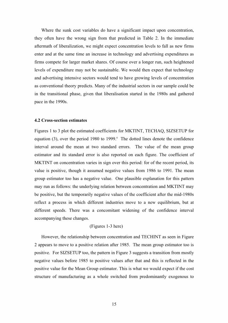
4.2 Cross-section estimates

Figures 1 to 3 plot the estimated coefficients for MKTINT, TECHAQ, SIZSETUP for

equation (3), over the period 1980 to 1999.4 The dotted lines denote the confidence

interval around the mean at two standard errors. The value of the mean group

estimator and its standard error is also reported on each figure. The coefficient of

MKTINT on concentration varies in sign over this period: for of the recent period, its

value is positive, though it assumed negative values from 1986 to 1991. The mean

group estimator too has a negative value. One plausible explanation for this pattern

may run as follows: the underlying relation between concentration and MKTINT may

be positive, but the temporarily negative values of the coefficient after the mid-1980s

reflect a process in which different industries move to a new equilibrium, but at

different speeds. There was a concomitant widening of the confidence interval

accompanying these changes.

(Figures 1-3 here)

However, the relationship between concentration and TECHINT as seen in Figure

2 appears to move to a positive relation after 1985. The mean group estimator too is

positive. For SIZSETUP too, the pattern in Figure 3 suggests a transition from mostly

negative values before 1985 to positive values after that and this is reflected in the

positive value for the Mean Group estimator. This is what we would expect if the cost

structure of manufacturing as a whole switched from predominantly exogenous to

16

endogenous sunk costs. One possibility is that liberalisation enabled easier imports of

capital goods and technology.

Interestingly, this explanation lends support to the thesis (see DeLong 2001) that

the reforms of the mid-1980s were more significant in terms of their impact on

economic activity than the much-emphasised reforms of 1991. To test if this is indeed

the case, we estimated (3) with fixed time and industry effects for the periods 1970-

84, 1985-99, 1991-99 and 1970-99. The results reported in Table 7 do indeed confirm

the change in underlying coefficient values after 1985. In particular, the relationship

between concentration and the size set-up ratio emerges as positive and significant in

the later period.

(Table 7 here)

5. Conclusion

Prior to liberalization, market structure in Indian manufacturing was largely an artifact

of government policy. This was hardly surprisingly given the nature and extent of

regulatory control. We would expect deregulation and liberalization to alter the

picture, though the precise effects could vary across industries. Concentration levels

may rise or fall depending on the specifics of individual sectors. The dynamic picture

within individual sectors could be complicated too, as deregulation alters the strategic

choices of incumbents and enables new entry. This variability suggests the need for a

sector-specific rather than general examination of the impact of deregulation on

concentration. Looking across sectors, we also find that concentration was more

affected by sunk cost variables in the period before 1991 than after.

The fact that implications of deregulation for concentration differ across sectors

strongly supports the need for a sector-specific approach to competition policy. While

this is quite common practice in developed countries, many developing economies

have yet to develop this approach. Recent discussions of the Competition Bill suggest

that India is taking the right path. A second implication suggested by our analysis in

Section 1 is that policy changes respond to increases in levels of concentration: in that

sense regulatory policy may have an element of ‘endogeneity’.

4 The full estimated equations corresponding to these are available from the authors.

17

References

Ahluwalia, I.J. (1985), Industrial Growth in India: Stagnation Since the Mid-1960s, Oxford University Press.

Athreye, S. and S. Kapur (2001), ‘Private Foreign Investment in India: pain or panacea?’ The World Economy, 24 (3), 399-424.

Basant, R. (2000), ‘Corporate Response to Economic Reforms’, Economic and Political Weekly, March 4, pp. 813-22.

Boyd, D. and R. Smith (2000), ‘Some Econometric Issues in Measuring the Monetary Transmission Mechanism with an Application to Developing Countries’, Discussion Papers in Economics No. 15/2000; Birkbeck College, London, UK.

Davies, S. and P. Geroski (1997), ‘Changes in Concentration, Turbulence, and the Dynamics of Market Shares’, Review of Economics and Statistics, 79, 383-91.

DeLong, B. (2001), ‘India since Independence: an analytic growth narrative’. Available online at ksghome.harvard.edu/~drodrik.academic.ksg/Growth%20volume/DeLong-India.pdf Gang, I. (1995), Small firms in India: a discussion of some issues, in D. Mookherjee(ed). Indian Industry: policies and performance, Delhi: Oxford University Press.

Kambhampati, U.S. (1996), Industrial Concentration and Performance: A Study of the Structure, Conduct and Performance of Indian Industry, Delhi: Oxford University Press.

Kambhampati, U. S. and P. Kattuman (2003), ‘Growth response to competitive shocks: Market structure dynamics under liberalization: the case of India’, working paper number 263, ESRC Centre for Business Research, University of Cambridge.

Sivadasan, J. (2002), ‘Regulatory regime in India: 1947 to 1998’, available at

http://home.uchicago.edu/~jmsivada/reg_history1.doc .

Smith, R. and M.H. Pesaran (1995), ‘Estimating long run relationships from dynamic heterogeneous panels’, Journal of Econometrics, 68, 79-113.

Sutton, J. (1991), Sunk Costs and Market Structure: Price Competition, Advertising, and the Evolution of Concentration. MIT Press

Sutton, J. (1998), Technology and Market Structure: theory and history. MIT Press

World Bank (1989), India: An Industrialising Economy in Transition, Washington DC: World Bank.

18

Table 1a: Key changes in India’s industrial policy regime, 1950-1980 Industries (Development and Regulation) Act, 1951

Specified the Schedule I industries where licenses were required for firms with fixed investment above a certain level of investment or import content of investment above a certain level

Companies Act, 1951 Restrictions on the operation of managing agencies, which affected the operation of many British companies in India

Industrial Policy Resolution, 1956

Articulated the role of public investment in planned development and specified: Schedule A industries reserved exclusively for state enterprises Schedule B industries where further expansion would be by state enterprises

Corporate Tax policies, 1957-1991

Specified rates of corporate tax on companies incorporated outside India. These were usually between 15-20% higher than the rates applied to large Indian companies during this period.

Monopolies and Restrictive Trade Practices Act, 1969

All applications for a license from companies belonging to a list of big business houses and subsidiaries of foreign companies were to be referred to a ‘MRTP Commission’ which invited objections and held public hearings before granting a license for production.

Industrial Policy Notification, 1973

Made licensing mandatory for all industries above certain investment limits Specified industry Schedules IV and V , where licensing was mandatory for all firms irrespective of size Small scale industry reservation introduced for some industries. Small was defined based on an investment limit.

Industrial Policy Statement, 1973

Specified the criteria and list of Appendix I of ‘core’ industries to which large business houses and foreign firms were to be confined. Main criteria for being an Appendix 1 industry were that of local non-availability or domination of a sector by a single foreign firm. Schedule A industries from IPR, 1956 could not figure in the Appendix 1 list.

Foreign Exchange Regulation Act, 1973

Foreign companies operating in India were required to educe their share in equity capital to below 40%. Exceptions were decided on a discretionary basis if: The company was engaged in ‘core’ activities ( as defined in IPS, 1973) The company was using sophisticated technology or Met certain export commitments

Industrial Policy Resolution 1977

Expanded the scope of reservations of particular lines of business activity for production in the small scale industrial sector. Small industry concessions would be lost if firm grew to a certain ‘large’ size.

19

Table 1b: Key changes in India’s industrial policy regime, 1980-1999

Policy announcements, 1985

Business houses were not restricted to Appendix 1 industries as long as they moved to industrially backward regions Minimum asset limit defining business houses was raised from Rs. 200 million to Rs. 1 billion

Amendment to MRTP Act, 1985

A company could be referred to the MRTP commission only if it showed assets greater than Rs. 1 billion.

New Industrial Policy 1991

Abolished licensing for all except 18 industries. Large companies no longer needed MRTP approval for capacity expansions Number of industries reserved for the public sector in Schedule A (IPR1951), cut down from 17 to 8; Schedule B was abolished altogether. Small firms were allowed to offer upto 24% of shareholding to large enterprises. Limits on foreign equity holdings were raised from 40 to 51% in a wide range of industries and foreign exchange outflows as dividends were balanced by export earnings. EXIM scrips (import entitlements linked to export earnings) were introduced and were freely tradable and could be used for all categories of imports. Actual user requirements for import of capital goods, raw materials and components under OGL were removed. Royalty limits increased to encourage technology imports.

Policy announcements, 1992-99

Number of industries requiring licensing steadily decreased. By 1998 the number of industries requiring compulsory licensing was down to 9. Oil exploration and Minerals were removed from list of reserved industries for the public sector, bringing the number of Schedule A industries down to 6. Infrastructure industries like basic telecom and power opened to private ownership (including foreign ownership). Small scale industry reservations decreased: 15 items including ready made garments are removed from reserved list. Investment limit for defining a firm as small scale raised from Rs. 7.5 million to Rs. 30 million. Pricing of coal, drugs and pharmaceuticals de-regulated.

Tariff reductions, 1992-99

Peak tariffs reduced to 110% in 1992 and gradually brought down to 40% in 1998. List of freely importable goods expanded Reform of structure of tariffs.

Source for Table 1: Adapted from Sivadasan, J. (2002), with authors’ additions.

20

Table 2: Variables used in the analysis and expected coefficient values

Variable Name

Relation to Equation (2) or (3)

Description Expected signs

HERF2 Cit HERF2(-1) Cit-1 Lagged value of the Herfindahl

index In equation (2) only (+) as 0 ≤ λ1 < 1

MKTINT W1it Value of industry’s marketing intensity; marketing intensity is total of all advertising and selling expenses as a percentage of industry sales

(+)

TECHACQ W2it Value of industry’s technology acquisition intensity; technology intensity is the sum of royalties paid (in rupees and foreign currency) + technology fees in foreign currency, by all firms in the industry as a percentage of total industry sales

(+)

SIZSETUP W3it Ratio of industry sales to average net fixed assets

(-) But can become positive in the presence of endogenous sunk costs

TIME T In equation (2) only Can take any sign.

NUMBER Control variable

The number of reporting firms in each year, controls for measurement errors of right hand side variable and spurious increases in the Herfindahl index due to under-reporting in certain years

(-) . Increasing numbers of firms decrease the Herfindahl index and vice versa.

21

Table 3: Variability between and within industries (1980-99)

Variable Mean Std dev Minimum Maximum

HERF2 Overall 31.840 26.489 1.101 100.00

Between 23.355 2.459 95.512

Within 12.393 -10.873 89.051

MKTINT Overall 1.642 1.647 0.000 12.618

Between 1.222 0.127 6.702

Within 1.078 -4.429 8.989

TECHACQ Overall 0.373 1.414 0.000 19.796

Between 1.246 0.002 9.138

Within 0.770 -5.299 11.030

SIZSETUP Overall 60.084 94.038 0.502 1112.769

Between 71.907 4.553 353.802

Within 59.852 -278.842 819.051

NUMBER Overall 18.112 24.328 1 249

Between 20.885 1.367 104.64

Within 12.525 -64.221 166.779

Notes: (i) The above figures are estimated by STATA.

(ii) The between mean is calculated over 53 industrial sectors and is x i. The within

mean is calculated as ( xit - x i + x ) where x is the global mean computed over 1441

observations.

22

Table 4: Descriptive statistics, dynamic model (1970-1999)

Cotton Wool Jute Auto Machine Chemical Variable Sugar Textiles Textiles Textiles

BreweryVehicles Tools Fertilisers

Dyes & Dyestuffs

Medicinal prep.

Cement Paper

HERF2 mean 4.325 6.928 30.458 6.857 20.170 18.058 22.789 15.798 18.462 4.306 16.446 9.611std devn 1.490 6.082 11.822 2.918 10.686 3.029 4.315 3.141 3.498 0.616 4.099 3.619Min 2.468 1.100 15.028 3.382 10.131 13.860 16.601 10.289 14.238 3.306 9.875 5.972max 8.412 20.650 64.255 12.609 47.407 25.048 32.933 20.223 29.237 5.353 23.265 22.186MKTINT mean 0.428 1.472 3.954 0.671 4.449 0.965 2.535 0.464 1.915 3.493 0.692 0.720std devn 0.106 0.482 0.634 0.129 1.856 0.482 1.051 0.374 0.334 0.629 0.337 0.382Min 0.241 0.924 2.956 0.414 2.250 0.312 1.019 0.120 1.136 2.612 0.325 0.294max 0.693 3.175 5.508 0.844 11.780 2.871 4.197 1.457 2.569 5.198 1.506 1.529TECHACQ mean 0.076 0.117 0.076 0.019 0.492 0.323 0.366 0.481 0.073 0.144 0.548 0.112std devn 0.067 0.225 0.151 0.032 0.585 0.194 0.369 0.632 0.079 0.186 0.326 0.135Min 0.000 0.000 0.000 0.000 0.000 0.000 0.000 0.000 0.000 0.000 0.000 0.000max 0.254 0.898 0.758 0.118 2.020 0.680 1.811 3.251 0.378 0.671 1.120 0.540SIZSETUP mean 147.242 353.802 23.518 110.940 56.968 61.430 33.147 29.651 31.187 269.186 35.794 57.521std devn 76.489 359.291 18.417 87.842 27.600 20.653 6.986 9.383 8.113 54.368 10.864 17.366Min 30.965 14.877 6.084 20.850 16.772 34.941 21.110 12.222 17.378 162.130 16.762 36.923max 270.574 1112.769 79.130 258.207 102.157 117.426 51.915 47.505 48.770 393.362 62.329 98.481NUMBER mean 45.900 100.333 8.330 24.867 19.467 19.933 11.433 18.433 12.800 63.333 24.967 39.533std devn 14.947 78.171 1.971 10.708 4.769 6.948 1.073 4.790 2.398 11.050 9.661 9.515Min 20.000 18.000 5.000 12.000 11.000 13.000 10.000 12.000 9.000 52.000 15.000 25.000max 70.000 249.000 13.000 42.000 28.000 34.000 13.000 29.000 16.000 89.000 45.000 62.000

Notes to Table 4: The industry group Cotton textiles was re-classified into finer categories in later years. The number of firms in initial years is thus quite large – 249 reporting firms from 1970-75, 113 reporting firms from 1975-80 and 91 reporting firms thereafter.

23

Table 5: Time series estimations for twelve industry groups (1970-99) Variable Sugar Cotton

Textiles Wool Textiles

Jute Textiles

Brewery Auto Vehicles

Machine Tools

Chemical Fertilisers

Dyes & Dyestuffs

Medicinal prep.

Cement Paper

Constant 7.096*** -12.352*** 28.667** 15.651*** 57.732*** 23.782*** 39.408*** 24.821*** 19.773*** 7.812*** 25.222*** 16.455** MKTINT 2.706** 0.857 3.053 -1.512 -0.026 -1.767*** -1.364** -1.706 -0.772 -0.204 -0.081 -4.422* TECHACQ -2.472 0.841 1.616 -9.689* 1.610 0.872 -3.359*** -0.270 -11.576 0.384 3.674*** -9.135 SIZSETUP 0.001 0.006 0.332* 0.005 -0.035 0.120*** 0.223*** -0.030 -0.201*** -0.003* -0.053 0.060 HERF2 0.006 0.094*** 0.684** 0.048* -0.021 0.069*** 0.214 -0.019* 0.405*** -0.021 0.026 0.237 TIME 0.032 0.891*** 0.007 -0.039 -0.600*** -0.022 0.005 -0.319** 0.167** -0.055** -0.318*** 0.112* NUMBER -0.097*** 0.013 -4.575** -0.318*** -1.364*** -0.638*** -2.134*** -0.103 -0.211 -0.016 -0.174** -0.258* Structural parameters λ 0.994 0.906 0.316 0.952 1.021 0.931 0.786 1.019 0.595 1.021 0.974 0.763 β1i 2.722 0.946 9.662 -1.588 -0.025 -1.897 -1.736 -1.674 -1.299 -0.200 -0.083 -5.799 β2i -2.487 0.928 5.113 -10.178 1.577 0.937 -4.274 -0.265 -19.468 0.376 3.770 -11.980

β3i 0.006 0.104 2.165 0.050 -0.021 0.074 0.273 -0.019 0.682 -0.021 0.026 0.311

Diagnostics R-squared 0.924 0.904 0.935 0.935 0.899 0.747 0.785 0.736 0.652 0.775 0.874 0.460 Adjusted R-squared 0.904 0.879 0.918 0.918 0.873 0.681 0.730 0.667 0.562 0.716 0.842 0.319 S.E. of regression 0.461 2.113 3.394 0.835 3.812 1.710 2.244 1.811 2.315 0.328 1.631 2.987 Sum squared resid 4.894 102.721 265.008 16.035 334.304 67.237 115.851 75.454 123.314 2.479 61.177 205.187 F-statistic 46.602 36.203 54.793 55.211 34.138 11.341 14.035 10.702 7.197 13.184 26.698 26.698 Prob(F-statistic) 0.000 0.000 0.000 0.000 0.000 0.000 0.000 0.000 0.000 0.000 0.000 0.000 Autocorrelation Durbin-Watson 1.604 1.871 1.315 1.825 0.586 2.140 1.385 1.488 1.800 1.152 0.780 1.950 LM test F-statistic

0.421 1.540 0.913 0.071 13.741*** 1.624 1.022 1.204 0.085 3.132** 0.128 0.139

24

Table 6: Dispersion of industry coefficients around mean value

Cotton Wool Jute Auto Machine Chemical Variable Sugar Textiles Textiles Textiles

BreweryVehicles Tools Fertilisers

Dyes & Dyestuffs

Medicinal prep.

Cement Paper

MKTINT Average value -0.722 Standard error 2.033 Z-values 3.061 1.212 3.408 -1.157 0.329 -1.412 -1.009 -1.351 -0.417 0.151 0.274 -4.067 TECHACQ Average value -2.276 Standard error 5.100 Z-values -2.026 1.287 2.062 -9.243 2.057 1.319 -2.913 0.177 -11.130 0.830 4.120 -8.689 SIZSETUP Average value 0.035 Standard error 0.138 Z-values -0.253 -0.248 0.077 -0.249 -0.289 -0.135 -0.032 -0.285 -0.456 -0.258 -0.308 -0.195

Notes: Computed from Table 5.

25

Table 7: Change in the long-term relationship between concentration and sunk cost variables

Coefficient S.Error significance

1970-84, N*T=649 constant 38.18 3.07 *** MKTINT 0.98 0.41 ** TECHACQ 3.07 1.01 *** SIZSETUP 0.00 0.01NUMBER -0.08 0.07Residual sum of squares 47949.38F (70, 578) 73.46 *** 1985-99, N*T=792 constant 34.60 3.04 *** MKTINT -0.14 0.40TECHACQ 2.96 0.41 *** SIZSETUP 0.04 0.02 * NUMBER -0.44 0.09 *** Residual sum of squares 74803.43F (70, 721) 63.48 *** 1991-99, N*T=474 constant 38.37 3.55 *** MKTINT -0.078 0.51 TECHACQ 2.80 0.50 *** SIZSETUP 0.10 0.03 *** NUMBER -0.81 0.16 *** Residual sum of squares 36888.74 F (64, 409) 50.91 *** 1970-99, N*T=1441 constant 36.49MKTINT 0.73 0.30 ** TECHACQ 2.89 0.43 *** SIZSETUP 0.27 0.11 ** NUMBER -0.28 0.05 *** Residual sum of squares 198829.70F (85,1355) 65.07Notes:

(i) The panel is unbalanced and we estimated equation (3) as a fixed effects model with industry and time effects, but do not report the time and industry dummies here.

(ii) Estimations done in STATA, wit the following syntax

xi: regress herf2 mktint techaq sizsetup number i.sic i.year

26

Appendix 1: A note on the firm level data used in the analysis

The Reserve Bank of India conducts censuses of the public and private limited companies at periodic intervals (typically every 5 years). We rely here on these unpublished data on medium and large non-government, non-financial, public limited companies (i.e. those quoted on the stock exchange). Summary statistics based on this data are published periodically as reports on the Finances of Medium and Large Public Limited Companies. The coverage of industrial sectors is not complete as the Annual Survey of Industries. The exclusion of small firms is not a serious omission: except in a handful of sectors (e.g. leather) they are unlikely to be the principal competitors of publicly listed firms. The exclusion of government-owned companies is more serious as, over time, they came to contribute a substantial fraction of manufacturing output in the economy. The exclusion of 'unlisted' companies misses out firms such as the automobile giant Maruti Udyog Ltd (owned by Suzuki, Japan and the Government of India).

The data is longitudinal and, as available for the period 1965-2001 as a sequence of surveys. For confidentiality of financial data, companies are identified by a company code rather than company names. Firms are assigned to a three-digit industry code based on their primary activity. Reporting of firms is not uniform across all years and so the number of firms in an industry also fluctuates due to reporting. The cross-section analysis used data on 53 industry groups. Industries that appeared to be miscellaneous groupings were deliberately excluded. The industry coverage of data improves in later years and complete data for all industries are available from 1983. Table A1: List of 53 industries used in the cross section regressions Industry code Description 310 Grains and Pulses 320 Edible vegetable and hydrogenated oils 331 Sugar 341 Cigarettes 342 Tobacco ( other than cigarettes) 351 Cotton textiles (spinning) 352 Cotton textiles (weaving) 353 Cotton textiles( composite) 354 Other cotton textiles 355 Jute textiles 356 Silk and Rayon textiles ( spinning) 357 Silk & Rayon textiles (weaving) 358 Silk &Rayon textiles( composite) 359 Woollen textiles 360 Ginning pressing and other textile products 370 Breweries and distilleries 380 Leather & leather products 410 Iron & Steel 420 Aluminium 441 Auto vehicles 442 Automobile components 443 Railway equipment

27

445 Cables 446 Dry cells 447 Electric lamps 449 Machine tools 450 Textile machinery 452 Steel tubes and pipes 453 Steel wire ropes 454 Steel forgings 456 Aluminium ware 461 Chemical fertilisers 462 Dyes and dyestuffs 463 Man made fibres 464 Plastic raw materials 466 Medicines and pharmaceutical preparations 467 Paints, varnishes and allied products 469 Industrial and medical gases 470 Matches 510 Mineral Oils 521 Cement ( hydraulic) 522 Asbestos and asbestos cement products 531 Structural clay products 532 Ceramics 541 Tyres and tubes 551 Paper 552 Products of pulp and board 553 Wood products, furniture and fixtures 561 Glass containers 571 Printing 572 Publishing 573 Printing, publishing and allied activities 580 Plastic products

28

Appendix 2: Order of integration, I(p), of the variables: summary of ADF tests Industry Model:

Intercept only

Model: Trend and intercept

HERF2 MKTINT TECHACQ SIZSETUP HERF2 MKTINT TECHACQ SIZSETUPSugar I(1) I(1) I(1) I(1) I(0) I(1) I(1) I(0) Cotton Textiles I(1) I(1) I(0) I(0) I(1) I(0) I(1) I(0) Woollen Textiles I(1) I(1) I(1) I(1) I(2) I(0) I(1) I(1) Jute textiles I(1) I(1) I(0) I(1) I(1) I(0) I(1) I(0) Breweries I(0) I(1) I(4) I(1) I(1) I(1) I(1) I(1) Auto Vehicles I(0) I(0) I(1) I(1) I(1) I(0) I(1) I(1) Machine Tools I(4) I(1) I(0) I(0) I(2) I(0) I(0) I(1) Chemical Fertilisers I(1) I(0) I(0) I(0) I(0) I(1) I(0) I(1) Dyes and Dyestuffs I(0) I(0) I(1) I(0) I(1) I(0) I(1) I(2) Medicinal preparations

I(1) I(0) I(1) I(0) I(1) I(0) I(2) I(2)

Cement I(1) I(1) I(1) I(1) I(1) I(1) I(0) I(0) Paper I(0) I(1) I(1) I(0) I(1) I(1) I(1) I(2) Printing, Publishing & allied activities

I(0) I(1) I(1) I(1) I(0) I(1) I(1) I(1)

Figure 1: Change in coefficient on marketing intensity (eqaution 3) overtime[Mean group estimator = -0.463, Std error= 2.13]

-10

-5

0

5

10

1980 1981 1982 1983 1984 1985 1986 1987 1988 1989 1990 1991 1992 1993 1994 1995 1996 1997 1998 1999

year

coef

ficen

t val

ues

Figure 2: Change in coefficient on technological intensity (equation 3) overtime[Mean group Estimator= 2.18, Standard Error=2.047]

-15

-10

-5

0

5

10

15

1980 1981 1982 1983 1984 1985 1986 1987 1988 1989 1990 1991 1992 1993 1994 1995 1996 1997 1998 1999

year

coef

ficen

t val

ues

Figure 3: Change in coefficent on the ratio of market size to set-up costs (equation 3) overtime[ Mean Group estimate=0.084, Standard error=0.135]

-0.3

-0.2

-0.1

0

0.1

0.2

0.3

0.4

0.5

0.6

1980 1981 1982 1983 1984 1985 1986 1987 1988 1989 1990 1991 1992 1993 1994 1995 1996 1997 1998 1999

year

coef

ficen

t val

ues