industrial cooling systems - wiley
TRANSCRIPT

APPLIED INDUSTRIAL ENERGY AND ENVIRONMENTAL MANAGEMENT
Z. K. Morvay, D. D. Gvozdenac
Part III:
FUNDAMENTALS FOR ANALYSIS AND CALCULATION OF ENERGY AND
ENVIRONMENTAL PERFORMANCE
1
Applied Industrial Energy and Environmental Management Zoran K. Morvay and Dusan D. Gvozdenac © John Wiley & Sons, Ltd
Toolbox 12
COOLING TOWERS
1. Mechanical Draft Water Cooling Tower Designs. These towers usually consist of a vertical shell
made of plastic or metal. Water is distributed near the top and falls to the collecting basin. It passes
through the air that flows from the bottom to the top by means of forced or induced draft fans. Only
cooling towers with induced fans are presented in Fig. 12.1. The inside of a mechanical-draft tower
may be filled with a spray of water droplets from nozzles or packed with plastic or ceramic filling
down which water cascades from the top to the bottom. In many cases, a combination of spray and
plastic or ceramic-filling is used.
Before being discharged into the atmosphere, the water-laden exhaust air passes through a drift
(spray) eliminator which removes the water droplets as they are carried along.
Air Out
Air In Air In
Water in
Water out
Cross Flow
Air Out
Water in
Water out
Eliminator
Counter Flow
FAN
Plastic Filling
Air in Air In
Sprinkler
Pipe
Collecting Basin
FAN
Eliminator
Elim
ina
tor
Elim
ina
tor
Sprinkler Pipe
Collecting Basin
Figure 12.1: Scheme of Counter Flow and Cross Flow Cooling Towers
Counter flow cooling towers have, theoretically, a uniform exit air wet bulb temperature. Cross
flow towers exhibit a large variation of exit air wet bulb temperature, which is responsible for further

Part III – Toolbox 12:
COOLING TOWERS 2
evaporation loss. In addition, cross flow towers require more airflow in order to meet the same
cooling capacity and overall evaporation losses are very slightly higher.
Cooling towers used for air-conditioning systems are often located on the top of buildings, and the
cross flow cooling tower usually has a lower profile, which lends itself better to architectural
treatment.
2. Principles for Operation Analysis. A cooling tower cools water by contacting it with the air and
evaporating some of the water. One or more axial or centrifugal fans move the air vertically up or
horizontally through the tower. Spraying the water through nozzles or splashing the water down the
tower from one baffle to another provides a large surface area of water.
The performance of cooling towers is often expressed in terms of range and approach (Fig. 12.2).
Cooling range is the temperature difference between the hot water coming to the cooling tower and
the temperature of the cold water leaving the tower. Approach is the temperature difference between
the temperature of the cold water leaving the tower and the surrounding air wet bulb temperature.
Both the range and approach must be greater than zero in normal cooling tower operation. Most
common values are approximately 5 oC for both. Designers use the parameters and geometry of the
cooling tower in order to achieve these temperature differences in practice. That these and other
parameters are traditionally present in the designer’s practice, does not imply that they are also the
best. Their impact is also very important for the size of a cooling tower and its price. Unfortunately,
economic parameters change over time. There is no doubt that an optimum exists but it is very
difficult to change it as it requires frequent alteration in cooling tower manufacturing technology. This
is, however, very expensive.
In the cooling tower, the transfer takes place from water to unsaturated air. There are two driving
forces for the transfer:
the difference in dry bulb temperatures, and
the difference in vapor pressures between water surface and unsaturated air.
These two driving forces when combined form the enthalpy potential.
Hot Water to
Cooling Tower
Cold Water from
Cooling Tower
All temperatures used are illustrative only and subject
to wide variation
Wet bulb
temperature
28
oC
32 oC
38 oC
Cooling
Range
Approach
Figure 12.2: Schematic Definition Explains the Terms Cooling Range and Approach
Above the wetted surface (Fig. 12.3), there is a film of air through which temperature and vapor
pressure gradients exist. In the immediate vicinity of the wetted surface, the air is saturated at ta,s, xa,s
and ha,s. The rate of diffusion of water vapor through the air film will be equal to the rate of
condensation or evaporation of water on the wetted surface. Because of the condensation or
evaporation process which occurs over the wetted surface, there is a difference in enthalpy between
unsaturated and saturated air (h - ha,s). This quantity is the Enthalpy Potential, and it is the driving
force for the total energy transfer process between water and unsaturated air.

Part III – Toolbox 12:
COOLING TOWERS 3
t [oC] x [kgw/kgda]
tw,s = ta,s
xa,s
xw,s = ∞
WETTED SURFACE
Water
tw, xw = ∞
tws, xws = ∞
Unsaturated Air
t, x, h
tas, xas
Figure 12.3: One of Possible Temperature and Concentration Profiles with Unsaturated Air over
Wetted Surface
The cooling tower calculation is based on the most generally accepted theory of the cooling tower
heat-transfer process developed by Merkel. This analysis is based upon enthalpy potential difference
as the driving force.
It is assumed that a film of air surrounds each particle of water, and the enthalpy difference
between the film and surrounding air provides the driving force for the cooling process. In its
integrated form the Merkel equation is:
pm
c
A
0 pm
c
t
t ai c
Ah
c
dAh
hh
dtL19.4
in
out
(12.1)
Where:
tin = water temperature entering the cooling tower, oC;
tout = water temperature leaving the cooling tower, oC;
hc = convection coefficient, kW/(m2 K);
hi = enthalpy of saturated air at water temperature, kJ/(kg of dry air);
ha = enthalpy of air, kJ/(kg of dry air);
cpm = mean specific heat of moist air, kJ/(kg K);
A = total area of wetted surface includes the surface area of water drops as well as
wetted slats or other fill material, m2;
L = water mass flow rate, kg/s.
4.19 = mean ratio between specific heats of water and air
The airflow rate (G) is not shown explicitly in the equation above, but implicitly it is in the
convection coefficient.
This method assumes that the temperature of the surface of the water droplets prevails throughout
the droplet. Actually, the interior of the droplet has a higher temperature than that of the surface, and
heat flows by conduction to the surface where the heat- and mass-transfer processes occurs.
Cooling tower designer and manufacturers often use the Number of Transfer Units (NTU) to refer
to the term pmc c/Ah . The higher the value of NTU, the closer the temperature of the water leaving
the cooling tower will come to the wet bulb temperature of the entering air. The NTU is one of the
performance indicators for cooling towers.
Figure 4 illustrates the water and air relationships and the driving potential that exists in the
cooling tower, where air flows in a parallel but opposite direction to the water flow. The water
operating line is shown by the line AB and is fixed to the inlet and outlet tower water temperature.
The air operating line begin at C, vertically below B (in h - t diagram, Fig. 4(a)) and at the point
having enthalpy corresponding to that of the entering wet-bulb temperature.
The slope of air–operating lines is 4.19 · L/G.

Part III – Toolbox 12:
COOLING TOWERS 4
Heat capacity is the amount of heat thrown away by the cooling tower. It is equal to the mass flow
rate of water circulated times the specific heat of water times the cooling range.
It is very important to stress that:
– The change in wet bulb temperature (due to atmospheric conditions) will not change the
cooling tower performance indicator NTU.
– The change in the cooling range will not change the cooling tower indicator NTU.
– Only the change of water and air flow will change the performance indicator NTU.
En
tha
lpy
, k
J/k
g
Air Operatin
g LineW
ater
Oper
atin
g Lin
e
Saturated Line
A
D
B
C
Temperature, oC Absolute Humidity [-]
En
tha
lpy
[k
J/k
g]
A
D
B
C
tintout
ha = Enthalpy of Air
hi = Enthalpy of Saturated Air at Water Temperature(a) (b)
Saturated Line
Wate
r Opera
ting L
ine
hi,in
ha,out
hi,out
ha,in
hi,in
ha,out
hi,outha,in
Air Operating Line
Figure 12.4: Water and Air Operating Lines in Enthalpy-Temperature and Enthalpy-Absolute
Humidity Diagrams
3. For the practical analysis of cooling tower operation, the following losses influencing the operation
have to be defined:
Blow-Down
Evaporating Loss
Drift Loss
Make-Up
Blow-Down is the continuous or intermittent wasting of a small fraction of circulating water in order
to prevent concentration of chemicals in water. The purpose of blow-down in water cooling apparatus
is to reduce soluble solids or hardness. This reduces the scale-forming tendencies of water. The blow
down loss is as follows:
WaterMakeUpWatergCirculatin
WaterMakeUp
TDSTDS
TDSLossnEvaporatioLossDownBlow (12.2)
where:
TDSMakeUp Water = Total Dissolved Solids in Make-Up Water (mg/l or ppm)
TDSCirculating Water = Total Dissolved Solids in Circulating Water (mg/l or ppm)
Solids may be present in suspension and/or in solution and they may be divided into organic and
inorganic matters. Total dissolved solids (TDS) are caused by soluble materials whereas suspended
solids (SS) are discrete particles which can be measured by filtering the sample through fine paper.
The electrical conductivity of a solution depends on the quantity of dissolved salts present and for
diluted solutions it is approximately proportional to the TDS content:
Part III – Toolbox 12:
COOLING TOWERS 5
]l/mg[TDS
]m/S[tyConductiviK (12.3)
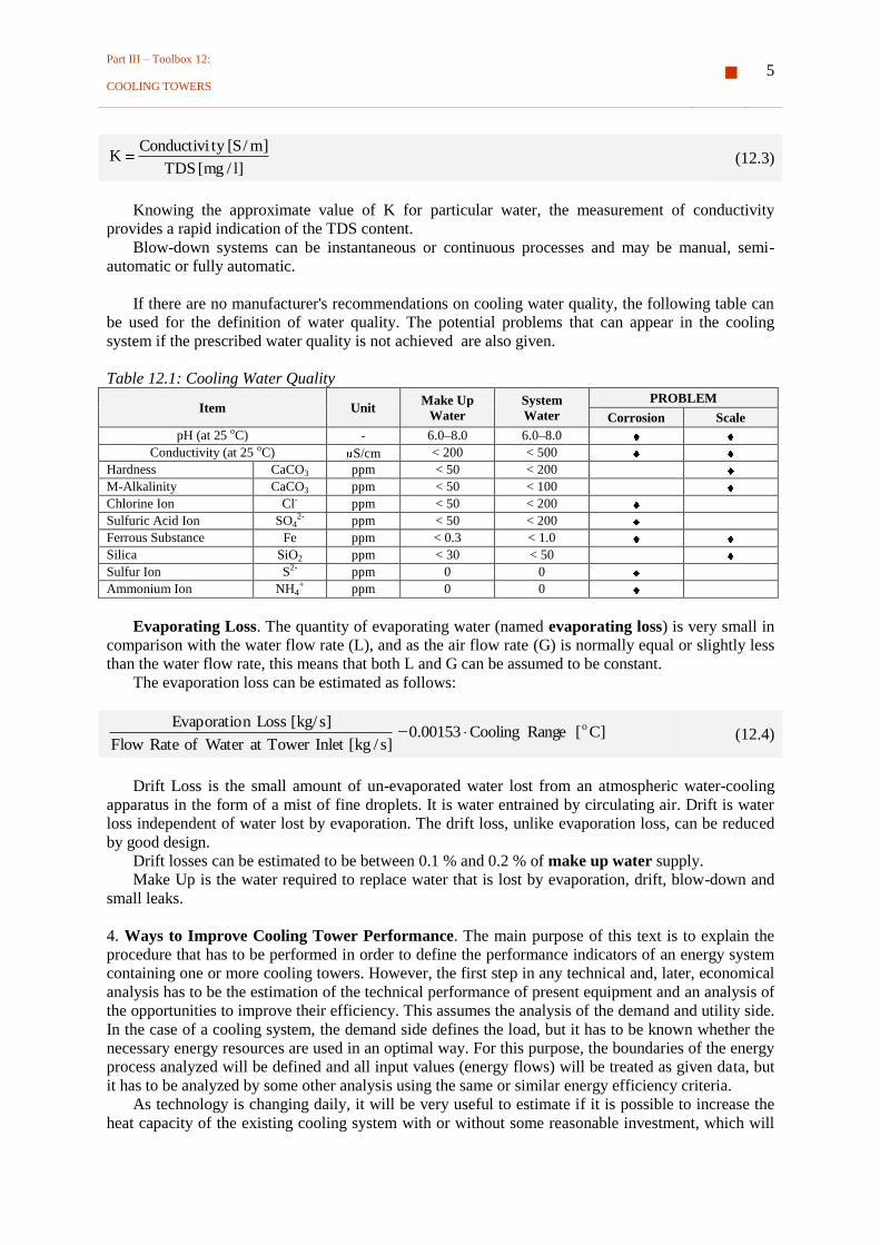
Knowing the approximate value of K for particular water, the measurement of conductivity
provides a rapid indication of the TDS content.
Blow-down systems can be instantaneous or continuous processes and may be manual, semi-
automatic or fully automatic.
If there are no manufacturer's recommendations on cooling water quality, the following table can
be used for the definition of water quality. The potential problems that can appear in the cooling
system if the prescribed water quality is not achieved are also given.
Table 12.1: Cooling Water Quality
Item Unit Make Up
Water
System
Water
PROBLEM
Corrosion Scale
pH (at 25 oC) - 6.0–8.0 6.0–8.0
Conductivity (at 25 oC) S/cm < 200 < 500
Hardness CaCO3 ppm < 50 < 200
M-Alkalinity CaCO3 ppm < 50 < 100
Chlorine Ion Cl- ppm < 50 < 200
Sulfuric Acid Ion SO42- ppm < 50 < 200
Ferrous Substance Fe ppm < 0.3 < 1.0
Silica SiO2 ppm < 30 < 50
Sulfur Ion S2- ppm 0 0
Ammonium Ion NH4+ ppm 0 0
Evaporating Loss. The quantity of evaporating water (named evaporating loss) is very small in
comparison with the water flow rate (L), and as the air flow rate (G) is normally equal or slightly less
than the water flow rate, this means that both L and G can be assumed to be constant.
The evaporation loss can be estimated as follows:
]C[RangeCooling00153.0]s/kg[InletToweratWaterofRateFlow
]s/kg[LossnEvaporatio o (12.4)
Drift Loss is the small amount of un-evaporated water lost from an atmospheric water-cooling
apparatus in the form of a mist of fine droplets. It is water entrained by circulating air. Drift is water
loss independent of water lost by evaporation. The drift loss, unlike evaporation loss, can be reduced
by good design.
Drift losses can be estimated to be between 0.1 % and 0.2 % of make up water supply.
Make Up is the water required to replace water that is lost by evaporation, drift, blow-down and
small leaks.
4. Ways to Improve Cooling Tower Performance. The main purpose of this text is to explain the
procedure that has to be performed in order to define the performance indicators of an energy system
containing one or more cooling towers. However, the first step in any technical and, later, economical
analysis has to be the estimation of the technical performance of present equipment and an analysis of
the opportunities to improve their efficiency. This assumes the analysis of the demand and utility side.
In the case of a cooling system, the demand side defines the load, but it has to be known whether the
necessary energy resources are used in an optimal way. For this purpose, the boundaries of the energy
process analyzed will be defined and all input values (energy flows) will be treated as given data, but
it has to be analyzed by some other analysis using the same or similar energy efficiency criteria.
As technology is changing daily, it will be very useful to estimate if it is possible to increase the
heat capacity of the existing cooling system with or without some reasonable investment, which will
Part III – Toolbox 12:
COOLING TOWERS 6
ultimately affect energy consumption. Actually, the first energy efficiency measure is to increase the
efficiency of the existing plant by improving the maintenance procedures and by implementing new
proven technology in the current energy system. Unfortunately, in many factories technical staff
hesitate to change to new technologies. Although they do not provide any technical parameters for
claiming that the existing technologies are successful, they fear the introduction of new technologies
because of lack of knowledge.
When the cooling tower load is exceeded, it is possible to install a second unit, install a larger
unit, or increase capacity of the existing cooling tower. The third option may give new life and
efficiency without requiring new, costly equipment.
If there is a need for more cooling tower capacity, but there is no room for a larger unit, the first
question is how to get more capacity out of the present cooling tower.
Cooling tower owners are often in trouble since many units serving power, process plants, or air-
conditioning systems are used for serving increased cooling loads as the plants have expanded.
However, many towers have not been able to keep up with actual plant operating conditions since
startup. This is not surprising when you realize that this type of equipment is often selected and
installed solely on a low first cost basis. As might be expected, a unit thus selected is very likely not
to be the most efficient or is even sometimes impractical for the job.
5. Increasing Capacity. Perhaps half of the field-erected and a few of the prefabricated towers
installed today can be improved to some degree. This is largely because of new technologies allowing
for more efficient components, and new materials that can be built into harder working, more rugged
and, therefore, more reliable packages.
Before trying to upgrade capacity, a complete study must be made of the cooling requirements.
Then, a careful inspection and analysis of the existing tower components is needed. This can be tied
together with respect to the existing tower size, pressure drop, airflow characteristics, drift loss, fan
performance curves, gear selection, service factors and installation problems.
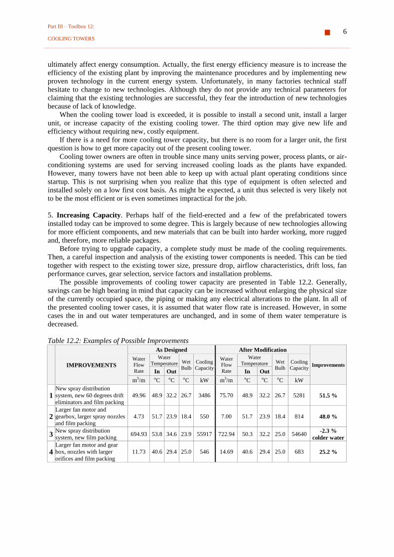
The possible improvements of cooling tower capacity are presented in Table 12.2. Generally,
savings can be high bearing in mind that capacity can be increased without enlarging the physical size
of the currently occupied space, the piping or making any electrical alterations to the plant. In all of
the presented cooling tower cases, it is assumed that water flow rate is increased. However, in some
cases the in and out water temperatures are unchanged, and in some of them water temperature is
decreased.
Table 12.2: Examples of Possible Improvements
IMPROVEMENTS
As Designed After Modification
Improvements
Water Flow
Rate
Water
Temperature Wet
Bulb
Cooling
Capacity
Water Flow
Rate
Water
Temperature Wet
Bulb
Cooling
Capacity In Out In Out
m3/m oC oC oC kW m3/m oC oC oC kW
1 New spray distribution
system, new 60 degrees drift
eliminators and film packing
49.96 48.9 32.2 26.7 3486 75.70 48.9 32.2 26.7 5281 51.5 %
2 Larger fan motor and
gearbox, larger spray nozzles
and film packing
4.73 51.7 23.9 18.4 550 7.00 51.7 23.9 18.4 814 48.0 %
3 New spray distribution
system, new film packing 694.93 53.8 34.6 23.9 55917 722.94 50.3 32.2 25.0 54640
-2.3 %
colder water
4 Larger fan motor and gear
box, nozzles with larger
orifices and film packing
11.73 40.6 29.4 25.0 546 14.69 40.6 29.4 25.0 683 25.2 %

Part III – Toolbox 12:
COOLING TOWERS 7
5
Fan motors increased from
29.4 t0 44.1 kW and larger
gearbox changed from high-
pressure spray to low-
pressure down spray type and
put in additional splash-type
fill
17.03 43.3 29.4 25.6 990 24.60 39.4 29.4 25.6 1030 4.0 %
colder water
6
Increased flume height of
tower by 5 m, new spray
distribution system, larger
motor, more splash-type fill
and tip seals placed in fan
stack
49.96 48.9 32.2 26.7 3486 84.03 48.9 32.2 26.7 5862 68.2 %
A cooling tower specialist should carry out studies and make recommendations. Once the findings
are acted upon in order to achieve practical results, substantial savings can be achieved and often save
on cost for a new unit.
6. The variables that influence cooling tower capacity and which have to be considered in order to
increase capacity are:
Fill Configuration
Distribution System
Drift Elimination
Mechanical Equipment
Fan Stack
Partitioning
Fill Configuration. Cooling tower packing has improved greatly over the years. When older
towers were originally installed, tower manufacturers designed the units to perform according to
specified conditions by using the type of packing that they considered to be the most economical for
their manufacturing facilities to produce. The design was, of course, consistent with the performance
and test data available at that time. Since then, improvements in design have come a long way, and
more field test data is currently available on different fill configurations.
For example, most old counter flow towers have splash type packing installed. Rows of splash
decks are usually spaced about 600 mm apart in the tower. The theory is to break up the water into
drops as it cascades through the tower. And each drop surface is increased by the continuous
interception of its fall by the splash decks, thus exposing a fresh evaporating surface on every new
drop.
Appraisal of the fill arrangement, and its quantity, by an experienced cooling tower specialist will
establish if more fill can be added in order to provide increased capacity. In this case, film surface
packing, or special packing that combines both film surface as well as additional splash surface is
installed. Some fill designs will increase the surface area and also the time that the water surface is
exposed to air. As a result, the rate of exposure may be high enough to permit the reduction of air
required. Therefore, film packing may be added without increasing fan horsepower requirements.
The percentage of capacity improvement that results from adding film surface-type fill depends
on the severity of the duty, the performance level and the height of the tower. For example, by adding
substantial quantities of film packing for a very low tower that is subjected to a very severe duty, 40
to 50 % capacity improvement can be obtained. On the other hand, if a very high tower is used for a
very easy duty, the performance can be adversely affected when film-type packing is installed. In this
instance, airflow rate is more critical to performance than the performance level itself.
However, for a reasonable performance level, a 20 % increase in capacity can be achieved for a
tower of average design. An increase of 20 % in capacity may be equated to a 20 % increase in the
water flow rate at the same temperature level, or an approximately 20 % decrease in the approach to
the wet bulb at the same flow rate and heat load.
Distribution System. Some older towers have open flume or trough distribution systems. This
type of system, especially in multi-cell installations, is hard to balance. The problem is then

Part III – Toolbox 12:
COOLING TOWERS 8
compounded when water loadings change in the process. Flooding or dry spots also detract from the
tower’s effectiveness.
Sometimes the gravity feed clogs at the downspouts. Each downspout has a diffusion deck, or
splash plate, under it. If these are broken or out of line, then the effective cooling volume is reduced.
Here, the change to a positive pressure spray-type distribution system reduces balancing problems. An
advanced design header-lateral spray system ensures a good water pattern over the entire fill area and
permits the passage of more air through this area of the tower.
Again, an analysis of the tower in operation reveals possible areas for improvement. Water spray
may not fully cover upper fill layers. Occasionally, water is halfway down through the fill before it is
evenly distributed across the entire plan area of the tower.
The obvious solution to this problem is to modify the nozzles so that the spray pattern is altered,
or corrected. This simple improvement often adds capacity to an existing tower.
Some older, high-pressure up spray towers have been converted to low-pressure down spray units
with improved results. This process entails raising the distribution system level, which permits
additional rows of fill decks to be installed. While this modification may increase capacity for as
much as 12 to 15 %, there will also be an overall, small decrease in pumping head.
Drift Eliminators. Many older towers have extra heavy drift eliminators. Others have close-
spaced eliminator blades of a 45o angle. Both designs are found to be too conservative for some
requirements. One reason is that these designs naturally restrict the air flow. By replacing them with
staggered drift eliminator blades at a 60o instead of a 45
o angle, more air is admitted through the tower
and the result is additional capacity.
Drift eliminator modifications are usually made when the drift eliminator requires replacement. A
counter flow tower improved by this simple change can increase capacity from 4 to 5 %. On a 5 oC
approach tower, this is equivalent to almost 0.5 oC colder water.
In some cases, an extra pass of drift eliminators can be installed in order to enable the change of
fan or gear to draw the maximum air flow rate without causing a drift loss problem.
Mechanical Equipment. If additional capacity is expected from the existing cooling tower, more
air movement is generally needed. But many installations already operate at the maximum rated
power. In such cases, additional readings have to be taken at the motor leads in order to determine
how close the motor is running to full load or nameplate amperage. If there is room for additional
load, the fan blade-angle has to be changed. Since power varies as the cube of airflow rate, nothing
much can be done without a larger motor.
Conversely, an increase in the air rate varies as the cube root of the increase in power. But a
substantial increase of power may lead only to a relatively small increase in capacity, as summarized
in Table 12.3.
Table 12.3: Motor Power versus Flow Rate
Motor Power Change
[kW]
Motor Power Change
[%]
Approximate Flow Rate
Change
[%]
25 to 30 20.0 6.0
30 to 40 33.3 10.0
40 to 50 25.0 7.5
50 to 60 20.0 6.0
60 to 75 25.0 7.5
75 to 100 33.3 10.0
If the unit is installed with the fan pitch angle at the maximum efficiency level, a change in fan
speed may be appropriate. Changing the gear ratio or motor achieves that.
Major modifications include increasing the fan size. But this is rarely done, as increasing the flow
rate by increasing fan speeds strains the limits of the tower from another viewpoint as a velocity that
is too high through the tower and drift eliminators can cause problems from excess carryover.
Full effectiveness can be realized from a larger motor with an increased pitch angle or fan speed.
Here, capacity improvement of as much as 10 % can be achieved.

Part III – Toolbox 12:
COOLING TOWERS 9
Fan Stack. The importance of fan stack design for top performance cannot be overemphasized. It
is not practical to change or increase the motor size on many existing units. One reason is that any
change of the electrical service to the cooling tower site might be unreasonably costly. Here, the
installation of a parabolic ventury-type fan stack may be the answer because, with this velocity
recovery-type fan stack, the fan is capable of delivering 6 to 7 % more air through the tower with the
same motor. 7 % more air means 7 % more tower capacity.
Partitioning. Some larger multi-cell towers are built for operation only at design load. Some of
these units have two fans per cell and there is no partition in the plenum area. If one fan is shut down
for repairs, or if the tower is operated with only one fan per cell for any reason, the mechanical draft
feature will be rendered practically ineffective. This is because the operating unit will then be drawing
most of its air through the adjacent fan opening, thus bypassing the fill area, which is extremely
wasteful.
But even if plenum areas are partitioned properly between fan cells (in counter flow towers) the
transverse partition should be extended down to the top of the louver level. Only then can the
effective counter flow principle be realized. If the unit is installed in a wide-open area, a longitudinal
partition has to be installed in order to prevent blow through when high winds hit at 90o to the
longitudinal axis of the tower. When the plant operates at partial load, proper partitions between fans
and cells will greatly improve operating efficiency.
7. Efficiency Obtained by Proper Operation and Maintenance. The cooling tower will be the
focus of more and more attention as increased effort is directed to the more efficient use and
conservation of water. The operating and maintenance manual for the cooling tower should be studied
by operating personnel in order to make sure that peak efficiency of the equipment is realized.
Consultations with a trained cooling tower engineer will enable the proper assessment of tower
components. The distribution system (air water pattern) is the key for the tower’s operating efficiency
and by an experienced survey the small difference needed to maintain the design capacity level may
be found. The dividends obtained by following such a procedure will more than justify the
comparatively small amount of time invested.
8. Energy Audit. The main purpose of an energy audit is to find opportunities to reduce energy
consumption and reduce energy costs. An energy audit is a process which can be divided into the
following steps:
Step 1: Boundary Identification and Physical Inspection
The first step in this process is to define the boundary of the system and establish the mass and energy
balances over the defined boundaries of the energy system. It includes the physical inspection of the
system and all the elements that form the system. An example of a cooling system is presented in Fig.
5. Three main parts can be identified:
– Cooling Tower System (within the boundary)
– Distribution System of Cooling Water
– End-users
The task of the cooling tower is simply to remove the heat generated by end-users. If the cooling
tower is ‘big’, it may accomplish the duty by cooling water temperature, for example, from 35 to 30 oC. If it is ‘small’, it may cool the water in the same process from 38 to 33
oC. In both cases, the heat
removed from the process to be cooled will be the same, if the flow rate is the same. The size of the
cooling tower, the flow rate and the wet bulb temperature determine the inlet and outlet water
temperatures, but not the difference between them.
In this phase of the system analysis, the measuring points have to be identified. In Fig. 12.5, the
following points are identified:
M1: Supply Water. The flow rate of water and its temperature has to be measured.
M2: Return Water. The temperature of return water has to be measured.
If measurements are performed, the heat capacity of cooling system will be:

Part III – Toolbox 12:
COOLING TOWERS 10
]C[TT)]Ckg/(kJ[19.4]s/kg[M]kW[Q oin,wout,w
ow (12.5)
For the proper operation of end-users, it is sometimes very important that the temperature of the
supply water is as designed.
The equation above defines the load of the system and it is obvious that the load varies with time
and depends on the processes that have to be cooled. Load versus time is the load profile and for any
energy analysis it must be defined.
MATRIXAmbient Air
Water
Exhaust Air
Waste Water
Electrical Energy
Boundary
M1
M5
M2
M3
M4
M6
Figure 12.5: Possible Scheme of Cooling System
M3: Ambient Air Parameters. In a cooling tower system water is cooled by moist air and,
because of that, the parameters of the air must be known. Of all moist air parameters, the most
important for cooling tower operation is wet bulb temperature. It is only wet bulb temperature that
strongly influences the enthalpy of air. The influence of other parameters such as dry bulb
temperature and pressure are within negligible ranges which occur in the normal operation of cooling
towers. The enthalpy of air versus wet bulb temperature is presented in Fig. 12.6.
The analytical relation of enthalpy versus wet bulb temperature can be represented by an
analytical expression as follows:
4.574424 t2.512014 t102.703963 - t101.618366 h WB2WB
-23WB
-3 (12.6)
The variation of ambient air parameters can be great during a day or month and will cause the
variation of cooling tower heat capacity and supply water temperature.
The flow rate of air has to be known as it influences the cooling tower’s heat capacity.

Part III – Toolbox 12:
COOLING TOWERS 11
0
20
40
60
80
100
120
140
160
10 15 20 25 30 35 40
Wet Bulb Temperature [oC]
Enth
alp
y o
f A
ir [
kJ/k
g]
Enthalpy of Air versus Wet Bulb Temperature
P = 1013 mbar
Figure 12.6: Enthalpy versus Wet Bulb Temperature (the Influence of Dry Bulb Temperature is
Negligible)
M4: Exhaust Air. The evaporation process within the cooling tower increases the absolute
humidity of exhaust air. Evaporation loss is practically the same for both counter- and cross- flow
cooling towers. As the air is almost saturated, the measurement of relative humidity or wet bulb
temperature is very difficult.
M5: Electrical Energy. Electrical energy is used for running the pump(s), fan(s) and auxiliary
equipment. The pump which runs water throughout the cooling tower is called the circulating pump.
The pump or pumps that are used for supplying end-users with cooling water are supply pumps and,
if there is a pump which returns the water from end-users to the cooling tower, it will be called the
return pump.
Most of the electrical energy is used for running the pumps. The power of a fan's electrical motor
is typically from 25 to 35 % of the circulating pump’s power.
M6: Waste water. The blow down is necessary in order to prevent the concentration of dissolved
solids from increasing to the point where it may precipitate and scale up heat exchangers and the
cooling tower fill, or reach unacceptable levels for other reasons.
Economics plays an important role in the selection of water treatment methods. It is possible to
prescribe ideal water for each cooling job, but the costs of equipment and chemicals are unacceptable
for most installations. So, treatment must be tailored to fit the size of any type of cooling-water
system currently in use.
The calculation of blow down is explained above, but the blow down loss is small compared to
the flow of circulating water flow.
During physical inspection, all of the relevant parts of the cooling tower system have to be
checked and repaired if necessary. In the previous section, all of the relevant elements are mentioned.
The potential measurement points and instrumentation have also to be checked. The methods of any
additional measurements necessary for energy audit have to be analyzed.
Step 2: Equipment Specification
An energy audit entails measurements, technical calculations and analysis. This means that a great
deal of technical data must be known. The most important thing is to know what are the design data
and/or standards for any measured and written value in the daily log sheets. This means that the
energy flows entering the boundary must always be known. The waste energy and material must also
be known.
The typical sets of data for any cooling tower are as follows:

Part III – Toolbox 12:
COOLING TOWERS 12
Name plate data Type of cooling tower
Manufacturer
Age
Type and characteristics of matrix
Design parameters:
- Water temperatures in tw,in oC
- Water temperatures out tw,out oC
- Mass flow rate of water L kg/s
- Wet bulb air temperature in ta,WB oC
- Mass flow rate of air G kg/s
Control system: ________________________________________________
Total annual operating time: ________________________________________
Total annual quantity of water supplied to the system: ____________________
Instrumentation and metering system: _______________________________
Housekeeping procedure: ___________________________________________
Water analysis report:
– pH = ____________
– Total dissolved solids of cooling tower water (TDSCTW) = _________
– Total dissolved solids of make-up water (TDSMuW) = ______________
Cooling tower fan:
– Mass flow rate of air
– Head of fan
– Power of electrical motor
– Type of fan
– Type of transmission
– Fan characteristics
Cooling tower pump (circulating pump):
– Mass flow rate of water
– Head of pump
– Power of electrical motor
– Type of pump
– Type of transmission
– Pump characteristics
Supply water pump
– Mass flow rate of water
– Head of pump
– Power of electrical motor
– Type of pump
– Type of transmission
– Pump characteristics
Step 3: Daily Log Sheets and Maintenance Records Analysis
The daily log sheet normally gives information on water temperature and pressure in and out, dry bulb
temperature and relative humidity or wet bulb temperature, and current (or electrical energy
consumption – kWh) of the electrical motors of the cooling system. In factories, regular water flow
measurements are rarely found and air flow measurements almost never.
Maintenance records provide the opportunity to estimate the condition of the analyzed energy
system. Preventive and regular maintenance always reduce maintenance costs significantly and
increase the reliability and prolong the lifetime of equipment.
Part III – Toolbox 12:
COOLING TOWERS 13
These matters have to be analyzed and improved within the implementation of the energy
management system.
Daily, weekly or/and monthly reports are desirable.
Step 4: Meteorological Data
Meteorological data could be very important for energy audit analysis. Many energy systems depend
strongly on meteorological data (heating, drying, air conditioning, etc.). In the case of cooling tower
systems the most dominant influence comes from the wet bulb temperature of the air. This value does
not vary by much. For example, the design wet bulb temperature in San Francisco and Bogota is 18 oC and for Hanoi is 30
oC. However, this value influences the dimensions dramatically and, later, the
operation of cooling towers.
These data can be obtained from a local meteorological institution.
Step 5: Measurements
The analysis performed during the realization of the actions described in Steps 1–3 has to be used for
the preparation of the measurement plan. How detailed the plan will be depends on the expected
results.
This means that in this phase the target must be clearly identified.
For example, if the water temperature difference is higher than designed, the cause can be a low
water flow rate, problems with the bed water spraying system, damage of the cooling tower filling,
increased load due to new machines installed, or a scaling problem at the machine heat exchanger,
etc. In this case, all potential causes must be checked and quantified. The water flow rate has to be
measured, the list of installed machines and their cooling load prepared and the spray system assessed
as either ‘poor’ or ‘good’, etc.
This procedure provides an opportunity to eliminate some of the causes and to solve the problems
of cooling system operation. All of these actions will result in energy efficiency improvement and, at
the same time, reduction in energy consumption.
The measurements necessary for cooling system analyses have already been defined in Step 1 and
presented pictorially in Fig. 12.5. The frequency of measurement, the type of instruments used, their
accuracy and the organization of measurements have to be the subject of independent analysis.
Step 6: Load Profile
A typical daily load is presented in Fig. 12.7. The presented heat load meets the real production
program. There is an automatic control system for the temperature of fluid to be cooled. The design
temperature of cooling tower water out is 32 oC and the design temperature difference is 5
oC.
However, as ambient parameters vary during the year, the load profile has to be defined for any
characteristic period of the year.

Part III – Toolbox 12:
COOLING TOWERS 14
0
500
1000
1500
2000
2500
1 2 3 4 5 6 7 8 9 10 11 12 13 14 15 16 17 18 19 20 21 22 23 24
Hour of Day
He
at
Lo
ad
[kW
]
Figure 12.7: Typical Load Profile
Step 7: Calculation and Analysis
It is very difficult to prescribe the types of calculation needed during an energy audit. But, it is
possible to identify the calculations that are used most often. As it has already been mentioned, the
energy audit is based on everyday measurements performed by technical staff and reported in daily
log sheets or by performing some advanced measurements prepared in advance with some special task
which will result in energy savings.
Software 10: Cooling Tower Calculation offers solutions to four problems for both counter or
cross flow cooling towers:
1. DETERMINATION OF PERFORMANCE INDICATORS
2. COMPARISON OF COOLING TOWER PERFORMANCE INDICATORS WITH
DESIGN DATA (ACCEPTANCE TEST)
3. INFLUENCE OF MASS FLOW RATES OF AIR AND WATER VARIATION
4. CALCULATION OF WATER MASS FLOW RATE FOR GIVEN LOAD AND WET BULB
TEMPERATURE
The cooling tower performance indicators are:
1. Number of Transfer Units (NTU):
m,p
c
c
AhNTU (12.7)
cp,m = mean isobaric specific heat of moist air, [kJ/(kg K)]
2. Heat capacity (Q):
]kW[TT19.4LQ in,wout,w (12.8)

Part III – Toolbox 12:
COOLING TOWERS 15
3. Range (r)
]C[TTr oout,win,w (12.9)
4. Approach (a)
]C[tTa oin,wb,aout,w (12.10)
5. Cooling degree ( CT)
][tT
TT
in,wb,ain,w
out,win,w
CT (12.11)
Step 8: Energy Conservation Opportunities
Generally speaking, after improving the existing cooling tower system by curing the deficiencies
found during the physical inspection of the site and satisfying optimal performance indicators, there
are only a few opportunities for reducing energy consumption:
a) Operational procedure improvement to meet the real load and design supply water
temperature
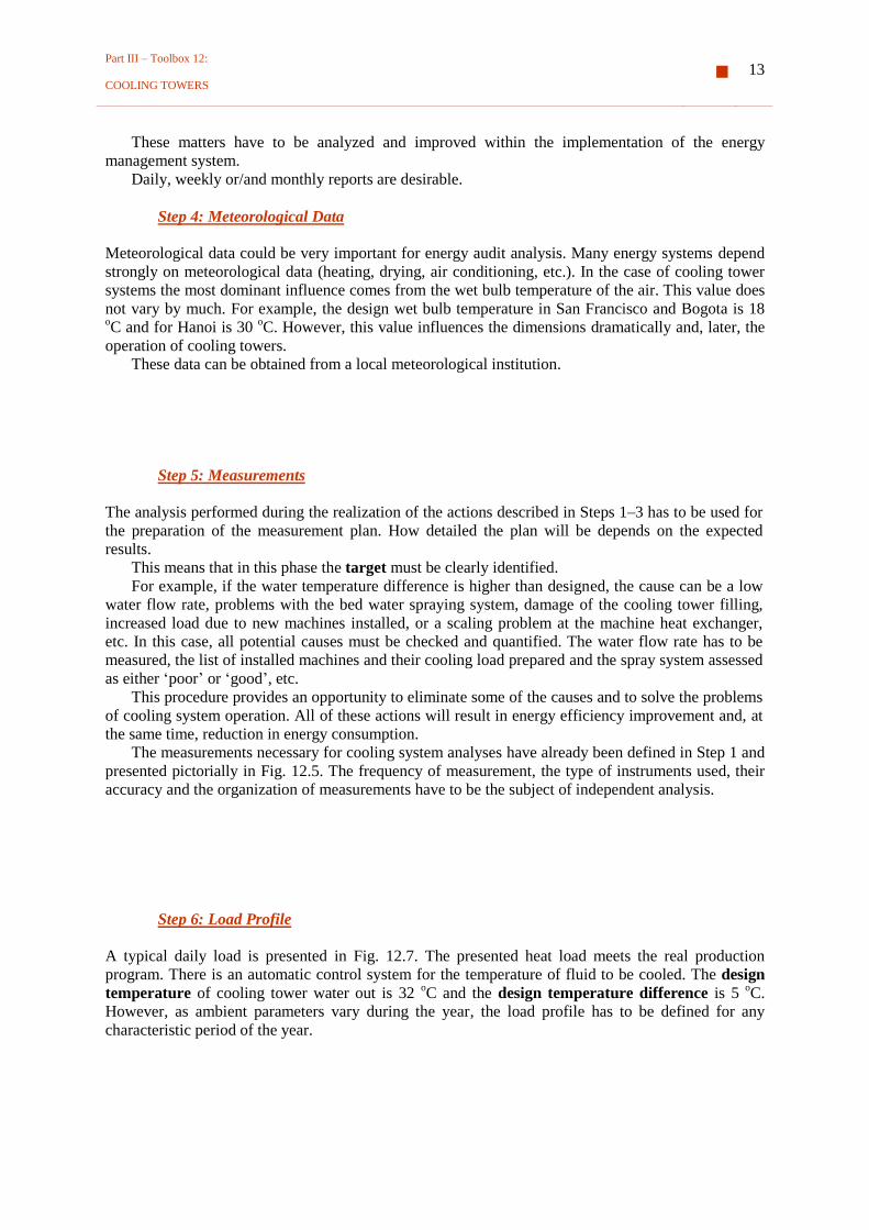
The ambient air wet bulb temperature will vary during the day and during the year. For any analysis
of the cooling tower system it has to be known in relation to weather conditions. The change of heat
capacity versus ambient wet bulb temperature for a particular counter flow cooling tower is presented
in Fig. 12.8. The outlet water temperature is also presented. In the case of more than one cooling
tower, sequential control has to be used. It can be done manually or automatically. For low wet bulb
temperatures often only one cooling tower will be enough. This procedure demands the measuring of
wet bulb temperature and load.
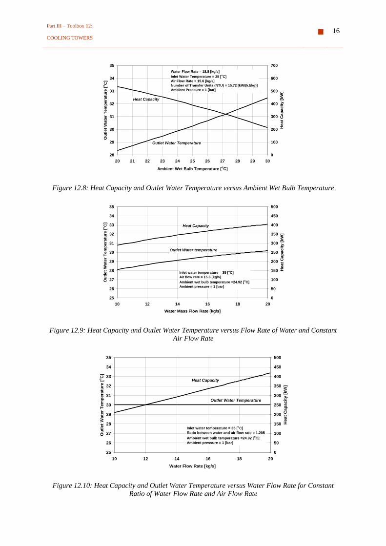
b) Implementation of variable speed drive control systems for pumps and fans
The more advanced technique used for adjusting the operation of cooling system to meet the real load
entails the implementation of variable speed drive control of pumps and fans.
The capacity of a cooling tower depends strongly on water and airflow rates (Figs 12.9 and
12.10).
c) Improvement of the control system and operational procedure of end-users
The analysis performed in this chapter assumes that the load is given. This means that the operation of
the end-users has not been subjected to analysis. However, it has to be stressed that the analysis of
end-users’ operation has also to be done. For example, in many industries there is no automatic
closing of cooling water valves when a machine is not in operation. If an electromagnetic valve is
installed, after stopping the machine the cooling water valve will be closed automatically or will be
closed after the time necessary for cooling the part of the relevant machine. If such valves are
installed, the load profile will be changed.
Part III – Toolbox 12:
COOLING TOWERS 16
28
29
30
31
32
33
34
35
20 21 22 23 24 25 26 27 28 29 30
Ambient Wet Bulb Temperature [oC]
Ou
tlet
Wate
r T
em
pera
ture
[oC
]
0
100
200
300
400
500
600
700
Heat
Cap
acit
y [
kW
]
Heat Capacity
Outlet Water Temperature
Water Flow Rate = 18.8 [kg/s]
Inlet Water Temperature = 35 [oC]
Air Flow Rate = 15.6 [kg/s]
Number of Transfer Units (NTU) = 15.72 [kW/(kJ/kg)]
Ambient Pressure = 1 [bar]
Figure 12.8: Heat Capacity and Outlet Water Temperature versus Ambient Wet Bulb Temperature
25
26
27
28
29
30
31
32
33
34
35
10 12 14 16 18 20
Water Mass Flow Rate [kg/s]
Ou
tle
t W
ate
r T
em
pe
ratu
re [
oC
]
0
50
100
150
200
250
300
350
400
450
500
He
at
Ca
pa
cit
y [
kW
]
Heat Capacity
Outlet Water temperature
Inlet water temperature = 35 [oC]
Air flow rate = 15.6 [kg/s]
Ambient wet bulb temperature =24.92 [oC]
Ambient pressure = 1 [bar]
Figure 12.9: Heat Capacity and Outlet Water Temperature versus Flow Rate of Water and Constant
Air Flow Rate
25
26
27
28
29
30
31
32
33
34
35
10 12 14 16 18 20
Water Flow Rate [kg/s]
Ou
tlet
Wa
ter
Te
mp
era
ture
[oC
]
0
50
100
150
200
250
300
350
400
450
500
Hea
t C
ap
acit
y [
kW
]
Inlet water temperature = 35 [oC]
Ratio between water and air flow rate = 1.205
Ambient wet bulb temperature =24.92 [oC]
Ambient pressure = 1 [bar]
Heat Capacity
Outlet Water Temperature
Figure 12.10: Heat Capacity and Outlet Water Temperature versus Water Flow Rate for Constant
Ratio of Water Flow Rate and Air Flow Rate

Part III – Toolbox 12:
COOLING TOWERS 17
Step 9: Financial Evaluation and Cost Benefit Analysis (see Toolbox 3)
This step will not be evaluated here. With precise technical and technological goals to improve
existing cooling tower energy efficiency, financial evaluation can be done in direct contact with
equipment manufacturers. With their prices and costs and financial capabilities, it is easy to prepare
the elements for a final decision.
9. Energy Audit Example
Step 1: Boundary Identification and Physical Inspection
Scheme of the System:
The boundaries of the system are presented in Fig. 12.11. At the same time, the measuring points are
also defined.
The overflow valve is opened if the pressure after the supply pump exceeds 5 barg. This has to
protect the pump from overloading.
A physical inspection will show that there is no visible damage to the system.
MATRIX
Ambient Air
Water
Exhaust Air
Waste Water
Electrical Energy
Boundary
M1
M2
M3
M4
M5
M6
Tw,in
[oC] Tw,out
[oC]
Figure 12.11: Scheme of the Cooling System

Part III – Toolbox 12:
COOLING TOWERS 18
Step 2: Equipment Specification
Cooling Tower Specifications (as designed):
LBC 600 – counter flow
Ambient wet bulb temperature = 28 oC
Water-in temperature = 37 oC
Water-out temperature = 32 oC
Water flow rate = 6736 l/min
Air flow rate = 3750 m3/min
Power of fan motor = 14.7 kW
Circulating Pump Specifications:
At working point (as designed):
Centrifugal
Flow rate = 112.3 l/s (6738 l/min)
Head = 25 mWC
Power of electrical motor = 39.33 kW
Speed = 1500 rpm
= 1.030623 10-3
V3 - 2.897075 10
-2 V
2 + 2.494792 10
-1 V + 1.382308 10
-2
H = -0.2125211 V2 +0. 6067072 V + 30.58355
N = -0.2616082 V2 + 5.427147 V + 14.64698
0
5
10
15
20
25
30
35
40
45
0 1 2 3 4 5 6 7 8 9
Volume Flow Rate [m3/min]
He
ad
[m
WC
] a
nd
Po
we
r [k
W]
0.0
0.1
0.2
0.3
0.4
0.5
0.6
0.7
0.8
0.9
Pu
mp
Eff
icie
nc
y [
-]
Head
Power
Efficiency
Figure 12.12: Head, Power and Pump Efficiency versus Volume Flow Rate of Circulating Pump

Part III – Toolbox 12:
COOLING TOWERS 19
0
5
10
15
20
25
30
35
40
0 1 2 3 4 5 6 7 8 9 10
Volume Flow Rate [m3/min]
He
ad
[m
WC
]
0
10
20
30
40
50
60
70
80
Po
we
r o
f E
lec
tric
al
Mo
tor
[kW
]
1500 rpm
1250 rpm
1000 rpm
750 rpm
500 rpm
Head
Power
Figure 12.13: Head and Power versus Volume Flow Rate of Circulating Pump for Different Speeds
Supply Water Pump Specifications:
At working point (as designed):
Centrifugal
Flow rate = 150 l/s (9000 l/min)
Head = 55.6 mWC
Power of electrical motor = 115.5 kW
Speed = 1750 rpm
Fluid temperature = from –15 to 180 oC
Maximum working pressure = 12 bar
Material = Cast iron casing
Inlet diameter = 250 mm
Discharge diameter = 200 mm
Impeller diameter = 342 mm
0
10
20
30
40
50
60
0
10
20
30
40
50
60
70
80
90
100
110
120
130
140
150
160
170
180
190
200
210
220
230
240
250
260
270
280
290
300
Flow Rate [l/s]
To
tal H
ead
[m
WC
]
1750 rpm
1600 rpm
1425 rpm
1200 rpm
960 rpm
Figure 12.14: Head versus Volume Flow Rate of Supply Pump for Different Speeds

Part III – Toolbox 12:
COOLING TOWERS 20
0
20
40
60
80
100
120
140
0
10
20
30
40
50
60
70
80
90
100
110
120
130
140
150
160
170
180
190
200
210
220
230
240
250
260
270
280
290
300
Flow Rate [l/s]
Sh
aft
Po
wer
[kW
]
1750 rpm
1600
1425 rpm
1200 rpm
960 rpm
Figure 12.15: Shaft Power versus Volume Flow Rate of Supply Pump for Different Speeds
0.0
0.1
0.2
0.3
0.4
0.5
0.6
0.7
0.8
0.9
1.0
0
10
20
30
40
50
60
70
80
90
100
110
120
130
140
150
160
170
180
190
200
210
220
230
240
250
260
270
280
290
300
Flow Rate [l/s]
Sh
aft
Eff
icie
ncy o
f P
um
p [
-]
17
50
rp
m
16
00
rp
m
14
25
rp
m
12
00
rp
m
96
0 r
pm
Figure 12.16: Efficiency versus Volume Flow Rate of Supply Pump for Different Speeds
Step 3: Daily Log Sheet and Maintenance Record
The system operates for 8000 hours annually. The production is more or less stable and varies from
75 to 90 % of installed capacity.
Daily log sheets contain the water temperature in and out and the pressure of water after the
supply pump. Only the current for the whole system is measured. These measurements show that
consumption is more or less constant.
Water and air flows have not been measured.
Water analysis has been performed once every day. pH and conductivity have been measured and
controlled. In compliance with performed measurements, chemicals have been added manually.
The water temperature after supply pump is approximately 32 oC and return water temperature
from end-users is approximately 35 oC. This means that the temperature difference is around 3
oC. As
the flow rate can be assumed to be constant (constant measured current), it can be concluded that the
supply water flow rate is greater than designed (5 oC).
From equipment specifications it can be recognized that the flow rate of the circulating pump is
6736 l/min and the supply water pump flow rate is 9000 l/min. There is no reason for the supply pump
flow rate to be greater than the circulating pump flow rate.
By inspecting the maintenance records, it is found that three years ago the supply pump was
replaced by a new one and it was decided then to buy a bigger pump for no special reason. After that
period, the temperature difference dropped from approximately 5 oC to 3
oC.
Part III – Toolbox 12:
COOLING TOWERS 21
The variation of the supply water temperature difference shows that there are significant
variations in the heat load.
There have been no complaints from production departments about the operation of the cooling
system. This means that during the whole year it has operated within the design’s anticipated ranges.
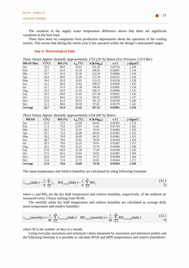
Step 4: Meteorological Data
These Values Appear Annually Approximately 1752 (20 %) Hours (For Pressure 1.013 Bar) MEAN Max T [oC] RH [%] twb [oC] h [kJ/kgda] x [-] [kg/m3]
Jan 32.0 89.0 30.41 101.59 0.02710 1.138
Feb 32.7 91.0 31.39 106.95 0.02891 1.134
Mar 33.7 91.0 32.36 112.50 0.03066 1.130
Apr 34.9 89.0 33.20 117.54 0.03213 1.124
May 34.0 92.0 32.81 115.13 0.03156 1.128
Jun 33.1 90.0 31.63 108.27 0.02926 1.133
Jul 32.7 91.0 31.39 106.95 0.02891 1.134
Aug 32.5 92.0 31.35 106.71 0.02890 1.135
Sep 32.3 94.0 31.45 107.30 0.02921 1.136
Oct 32.0 94.0 31.16 105.67 0.02870 1.137
Nov 31.6 91.0 30.33 101.13 0.02709 1.140
Dec 31.3 88.0 29.59 97.26 0.02570 1.142
Average 32.7 91.0 31.42 107.25 0.02901 1.134
These Values Appear Annually Approximately 5256 (60 %) Hours MEAN t [oC] RH [%] twb [oC] h [kJ/kgda] x [-] [kg/m3]
Jan 25.9 71.0 22.00 64.05 0.01491 1.170
Feb 27.4 75.0 23.97 71.61 0.01726 1.162
Mar 28.7 75.0 25.16 76.54 0.01866 1.156
Apr 29.7 75.0 26.08 80.50 0.01981 1.152
May 29.2 78.0 26.09 80.53 0.02002 1.153
Jun 28.7 78.0 25.62 78.50 0.01943 1.156
Jul 28.3 78.0 25.25 76.91 0.01897 1.157
Aug 28.1 79.0 25.21 76.76 0.01899 1.158
Sep 27.8 82.0 25.38 77.44 0.01938 1.159
Oct 27.6 81.0 25.04 76.03 0.01891 1.160
Nov 26.9 76.0 23.66 70.37 0.01698 1.164
Dec 25.6 71.0 21.73 63.05 0.01464 1.171
Average 27.8 76.6 24.60 74.36 0.01816 1.160
The mean temperature and relative humidity are calculated by using following formulae:
8
1n
nmean
8
1n
nmean RH8
1)daily(RHt
8
1)daily(t
(12.1
2)
where tn and RHn are the dry bulb temperature and relative humidity, respectively, of the ambient air
measured every 3 hours starting from 00:00.
The monthly mean dry bulb temperature and relative humidity are calculated as average daily
mean temperature and relative humidity:
M
1m
mean,mmean
M
1m
mean,mmean )daily(RHM
1)monthly(RH)daily(t
M
1)monthly(t
(12.1
3)
where M is the number of days in a month.
Using everyday maximum and minimum values measured by maximum and minimum probes and
the following formulae it is possible to calculate MAX and MIN temperatures and relative humidities:

Part III – Toolbox 12:
COOLING TOWERS 22
M
1m
MAX,mMAX
M
1m
MAX,mMAX )daily(RHM
1)monthly(RH)daily(t
M
1)monthly(t
(12.1
4)
M
1m
MIN,mMIN
M
1m
MIN,mMIN )daily(RHM
1)monthly(RH)daily(t
M
1)monthly(t
(12.1
5)
These Values Appear Annually Approximately 1752 (20 %) Hours
MEAN Min t
[oC]
RH
[%]
twb
[oC]
h
[kJ/kgda]
x
[-]
[kg/m3]
Jan 21.0 48.0 14.31 39.94 0.00741 1.194
Feb 23.3 54.0 17.14 47.92 0.00962 1.183
Mar 24.9 55.0 18.65 52.58 0.01081 1.176
Apr 26.1 55.0 19.67 55.89 0.01162 1.171
May 25.6 60.0 20.05 57.16 0.01232 1.172
Jun 25.4 62.0 20.19 57.63 0.01259 1.173
Jul 25.0 62.0 19.84 56.45 0.01229 1.175
Aug 24.9 63.0 19.90 56.67 0.01241 1.175
Sep 24.6 64.0 19.79 56.29 0.01239 1.176
Oct 24.3 64.0 19.52 55.41 0.01216 1.178
Nov 23.1 58.0 17.58 49.24 0.01022 1.184
Dec 20.8 51.0 14.59 40.68 0.00778 1.195
Average 24.1 58.0 18.44 52.15 0.01097 1.179
It is estimated that MAX mean and MIN mean temperatures and relative humidities appear
approximately 1752 hours per year and mean ones approximately 4256 h/year.
Step 5: Target Setting and Measurements
The previous analysis shows that there are no significant technical problems in the operation of the
analyzed system. However, the electrical energy consumption of this system is estimated to be
approximately 5 % of the total electrical energy consumption. The estimation is based on
measurements of the total electrical energy consumption (what is paid) and the electrical energy
consumed by this system and the compressed air system (which is on the side of the end-users of the
cooled water) as they have a kWh meter. The participation of this system in electrical energy
consumption is estimated on the installed power of both systems.
The main targets of the energy audit are formulated as follows:
Improve the efficiency of the system by implementing the Variable Speed Drive (VSD)
control system in both the pumps and the fan.
Analyze the possible consequences for the operations of end-users that can be produced by
the implementation of VSD control.
The basic assumptions of the technical and financial analysis are:
The load will not be changed in the near future.
The price of electricity will not change in the next 2–3 years.
The following plan for measurement is prepared (readings or measurements are done hourly):
Cooling Tower
Water flow measurement of circulating water
Water temperature in
Water temperature out
Air flow measurement
Dry bulb temperature measurement
Relative humidity of ambient air
Pressure of air

Part III – Toolbox 12:
COOLING TOWERS 23
Supply Water System
Water flow measurement of supply pump
Supply water temperature
Return water temperature
The list of instruments is not presented. The standard equipment is used.
The results are shown in the form of a graph in Figs 12.17–12.22. Figure 12.17 shows the dry and
wet bulb temperatures. It is easy to conclude that the wet bulb temperature (which is the most
important for cooling tower operation) is very stable. The mean value is 26.6 [oC]. This temperature is
quite high generally speaking, but for the area of Bangkok (Thailand), it is so very often (the designed
wet bulb temperature for Bangkok is 28 oC).
The air flow rate (Fig. 12.18) is measured by an anemometer. The velocity of the air is measured
at 24 points around the cooling tower suction area. The average velocity is multiplied by area and
density to get the average air flow rate. The average flow rate is 72.0 [kg/h] with StDev = 5.1 [kg/s] or
7.1 [%].
The average supply water flow is 141.1 [kg/s] (Fig. 12.19) with a standard deviation of 4.4 [kg/s].
The StDev is only 3.1 [%] and can be the error of measurement. Error includes both instrumentation
errors and errors of method. The power of the electrical motor is not measured.
The average circulating water flow (Fig. 12.21) is 110.0 [kg/s] with a standard deviation of 2.5
[kg/s] or 2.8 %. The power of the electrical motor is not measured. The comment on this measurement
is the same as for supply water measurement.
The temperatures of water are measured by immersing the thermometer (thermocouple). The bush
is installed in the pipeline after the supply water pump and return water tank. The circulated water
temperature is measured in the same way after the circulating pump and in the collecting basin at the
bottom of the cooling tower (Figs 12.21 and 12.22).
Average values are used for further calculations because the variation of flow measurements is
not significant and can be within the range of measurement errors. This means that it is not possible to
find a correlation between measured flow rates, measurement errors and what happens on the side of
end-users.
0
5
10
15
20
25
30
35
40
0:0
0
1:0
0
2:0
0
3:0
0
4:0
0
5:0
0
6:0
0
7:0
0
8:0
0
9:0
0
10
:00
11
:00
12
:00
13
:00
14
:00
15
:00
16
:00
17
:00
18
:00
19
:00
20
:00
21
:00
22
:00
23
:00
0:0
0
Time [hh:mm]
Dry
an
d W
et
Bu
lb T
em
pera
ture
[oC
]
Dry
Wet
P = 1.013 [bar]
Average 31.6 [oC]
Average 26.6 [oC]
Figure 12.17: Dry and Wet Bulb Temperature of Ambient Air

Part III – Toolbox 12:
COOLING TOWERS 24
0
10
20
30
40
50
60
70
80
90
1 2 3 4 5 6 7 8 9 10 11 12 13 14 15 16 17 18 19 20 21 22 23 24
Time [hh]
Air
flo
w r
ate
[k
g/s
] Mean Air Flow Rate = 72.0 [kg/s]
Figure 12.18: Air Flow Rate versus Time
0
20
40
60
80
100
120
140
160
1 2 3 4 5 6 7 8 9 10 11 12 13 14 15 16 17 18 19 20 21 22 23 24
Time [hh]
Su
pp
ly W
ate
r F
low
Ra
te [
kg
/s]
Mean Supply Water Flow Rate = 141.8 [kg/s]
Figure 12.19: Supply Water Flow Rate versus Time
20
22
24
26
28
30
32
34
36
38
40
1 2 3 4 5 6 7 8 9 10 11 12 13 14 15 16 17 18 19 20 21 22 23 24
Time [hh]
Su
pp
ly a
nd
Re
turn
Wa
ter
Te
mp
era
ture
s [
oC
]
Mean Supply Water Temperature = 31.6 [o
C]
Mean Return Water Temperature = 34.3 [o
C]
Figure 12.20: Supply Water Temperature In and Temperature Difference versus Time

Part III – Toolbox 12:
COOLING TOWERS 25
0
20
40
60
80
100
120
1 2 3 4 5 6 7 8 9 10 11 12 13 14 15 16 17 18 19 20 21 22 23 24
Time [hh]
Cir
cu
late
d w
ate
r fl
ow
ra
te [
kg
/s] Mean Circulated Water Flow Rate = 110.0 [kg/s]
Figure 12.21: Circulated Water Flow Rate versus Time
20
22
24
26
28
30
32
34
36
38
40
1 2 3 4 5 6 7 8 9 10 11 12 13 14 15 16 17 18 19 20 21 22 23 24
Time [hh]
Cir
cu
late
d w
ate
r te
mp
era
ture
in
/ou
t [o
C]
Mean Water Temperature OUT = 30.7 [o
C]
Mean Water Temperature IN = 34.3 [o
C]
Figure 12.22: Circulated Water Temperature Out and Temperature Difference versus Time
Finally, the values relevant for further calculation are:
Mass flow rate of circulated water (L) = 110.0 [kg/s]
Temperature of circulated water in (Tcw,in) = 34.3 [oC]
Temperature of circulated water out (Tcw,out) = 30.7 [oC]
Mass flow rate of air (G) = 72.0 [kg/s]
Wet bulb temperature (twb) = 26.6 [oC]
Mass flow rate of supply water (Msw) = 141.8 [kg/s]
Temperature of supply water in (Tsw,in) = 31.6 [oC]
Temperature of supply water out (Tsw,out) = 34.3 [oC]
Step 6: Load Profile
The load profile represents the heat energy removed from process versus time. For the analyzed case
it is presented in Fig. 12.23. This heat load meets the real production program. The water flow is
controlled manually before the water enters the machine. There are no electromagnetic valves in front
of the machines which will be closed when the machine is not in operation. The design temperature of
the water-in is 32 oC and the temperature difference is 5
oC.
If the load is split into 12 intervals starting from 900 kW by steps of 100 kW, it is possible to
calculate the frequency of load appearance over 24 hours. It is presented in Fig. 12.24. The maximum

Part III – Toolbox 12:
COOLING TOWERS 26
load (1950–2100 kW) appears approximately 30 % of time and the rest of the time system operates
with a load lower than maximum.
The average daily load is 1562.5 kW. As the cooling tower operates with a maximum water flow
rate this means that the temperatures of water in and out will be lower proportionally to the real load.
0
500
1000
1500
2000
2500
1 2 3 4 5 6 7 8 9 10 11 12 13 14 15 16 17 18 19 20 21 22 23 24
Hour of Day
Heat
Lo
ad
[kW
]
Figure 12.23: Daily Load
0
2
4
6
8
10
12
14
16
18
900-1
000
1000-1
100
1100-1
200
1200-1
300
1300-1
400
1400-1
500
1500-1
600
1600-1
700
1700-1
800
1800-1
900
1900-2
000
2000-2
100
Load [kW]
Fre
qe
nc
y o
f L
oa
d A
pp
ea
ran
ce
[%
]
Figure 12.24: Frequency of Load Appearance during the Day
Step 7: Calculation and Analysis
For the following measurement data:
pa = 1.013 bar
L = 110 kg/s
Tw,in = 34.30 oC
Tw,out = 31.60 oC
G = 72.00 kg/s
tdb,in = 31.60 oC
RHin = 68.2 %
by using Software (PROBLEM 1) it is possible to calculate the following cooling tower performance
indicators:
NTU = 51.78 kW/(kJ/kg)

Part III – Toolbox 12:
COOLING TOWERS 27
Q = 1244.43 kW
Cooling degree = 0.351
Range = 2.7 oC
Approach = 5.0 oC
By using NAME PLATE data (PROBLEM 2) and the already calculated NTU, the measured flow
rates and design temperature of air and water and a capacity of the cooling tower of 1562.53 kW are
obtained. This means that the actual capacity is lower by 33.6 % than that designed. The acceptance
test shows that the manufacturer delivered a cooling tower with a lower capacity. But, as the
guarantee period has expired, it is decided to accept the real capacity and to continue with the energy
audit.
Step 8: Energy Conservation Opportunities
ECO1: Increasing the air flow rate
The ratio is L/G = 1.53. It is decided to increase the flow rate of the fan from 72 kg/s to 90 kg/s by
replacing the electrical motor and transmission. The new ratio L/G will be 1.22. However, the
capacity of the cooling tower will increase from the current 1244.43 kW to 1431.89 kW (13.1 %). The
new NTU will be 60.80 kW/(kJ/kg).
ECO2: VSD control of pumps and fan
It is estimated that the most promising measure for the reduction of energy consumption is the
implementation of a variable speed drive for both pumps and the fan because:
a. The maximum load appears during only 30 % of the operating time. For the rest of the
operating time, the pumps can operate the system with much lower flows.
b. The supply pump is bigger than it is necessary and expends more energy for circulating
water around the network with a low temperature difference. This can be solved by
closing the proper valve but the energy consumption will be approximately the same.
c. All end-users are designed to operate with a supply water temperature of 32 oC and a
temperature difference of 5 oC.
The scheme of the cooling system with new VSD control systems is presented in Fig. 12.25.

Part III – Toolbox 12:
COOLING TOWERS 28
MATRIX
Tw,in
[oC] Tw,out
[oC]
VSD
controler
Three
phase
supply
VSD
controler
Three
phase
supply
Supply water
temperature 32 oC
Return water
temperature 37 oC
]C[5Tw o
]C[32out,Tw o
VSD
controler
Three
phase
supply
L/G = const.
Figure 12.25: Proposed Scheme of the Cooling System
The sensors for supply and return water temperature signal the temperatures to the controller
where the difference is calculated (the set temperature difference is 5 oC). The controller responds to
this temperature difference and adjusts the pump flow rate.
At the same controller of the circulating pump, the cooling tower flow rate is adjusted to
correspond to the outlet temperature of 32 oC. The controller of the fan follows the circulating pump
flow rate to keep the L/G ration on 1.22. The positioner for this control system produces the signal
proportional to the water flow rate and uses this signal to adjust the air flow rate in order to keep the
ratio L/G constant. Some of the details of the control systems can be and have to be discussed with the
manufacturers directly.
In the current case, the energy consumption can be estimated as follows:
]kWh[240,356,1000,85.11533.397.14ECurrent (12.16)
However, in the case where the system reacts to the ambient wet bulb temperature and changes
the load, the energy consumption calculation is more complicated. One possible approach is as
follows:
(a) The ambient air parameters relevant to the calculation of energy consumption are:
MAX mean (1752 hours per year):
tdb = 32.7 oC twb = 31.42
oC
MEAN (5256 hours per year):
tdb = 27.8 oC twb = 24.6
oC
MIN mean (1752 hours per year):
tdb = 24.1 oC twb = 18.44
oC
Part III – Toolbox 12:
COOLING TOWERS 29
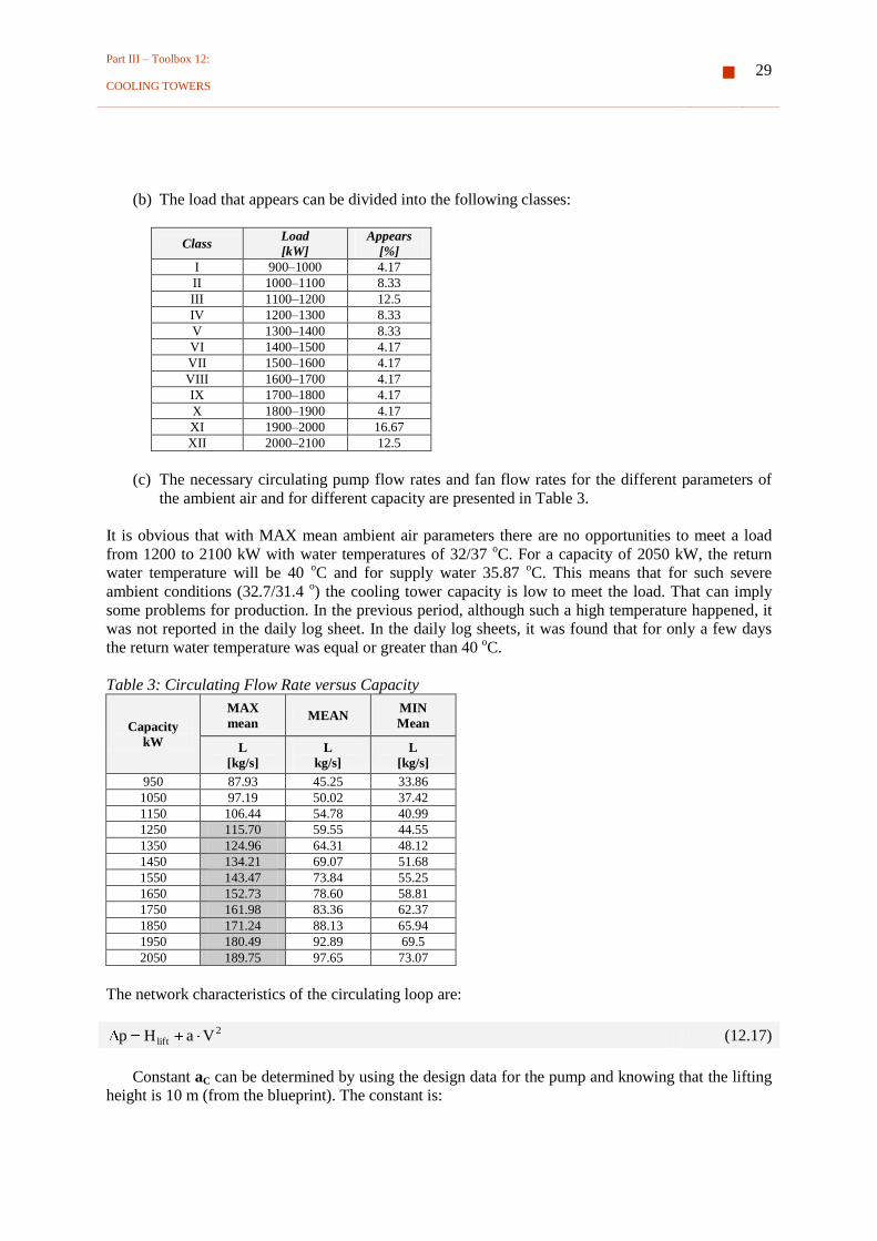
(b) The load that appears can be divided into the following classes:
Class Load
[kW]
Appears
[%]
I 900–1000 4.17
II 1000–1100 8.33
III 1100–1200 12.5
IV 1200–1300 8.33
V 1300–1400 8.33
VI 1400–1500 4.17
VII 1500–1600 4.17
VIII 1600–1700 4.17
IX 1700–1800 4.17
X 1800–1900 4.17
XI 1900–2000 16.67
XII 2000–2100 12.5
(c) The necessary circulating pump flow rates and fan flow rates for the different parameters of
the ambient air and for different capacity are presented in Table 3.
It is obvious that with MAX mean ambient air parameters there are no opportunities to meet a load
from 1200 to 2100 kW with water temperatures of 32/37 oC. For a capacity of 2050 kW, the return
water temperature will be 40 oC and for supply water 35.87
oC. This means that for such severe
ambient conditions (32.7/31.4 o) the cooling tower capacity is low to meet the load. That can imply
some problems for production. In the previous period, although such a high temperature happened, it
was not reported in the daily log sheet. In the daily log sheets, it was found that for only a few days
the return water temperature was equal or greater than 40 oC.
Table 3: Circulating Flow Rate versus Capacity
Capacity
kW
MAX
mean MEAN
MIN
Mean
L
[kg/s]
L
kg/s]
L
[kg/s]
950 87.93 45.25 33.86
1050 97.19 50.02 37.42
1150 106.44 54.78 40.99
1250 115.70 59.55 44.55
1350 124.96 64.31 48.12
1450 134.21 69.07 51.68
1550 143.47 73.84 55.25
1650 152.73 78.60 58.81
1750 161.98 83.36 62.37
1850 171.24 88.13 65.94
1950 180.49 92.89 69.5
2050 189.75 97.65 73.07
The network characteristics of the circulating loop are:
2
lift VaHp (12.17)
Constant aC can be determined by using the design data for the pump and knowing that the lifting
height is 10 m (from the blueprint). The constant is:
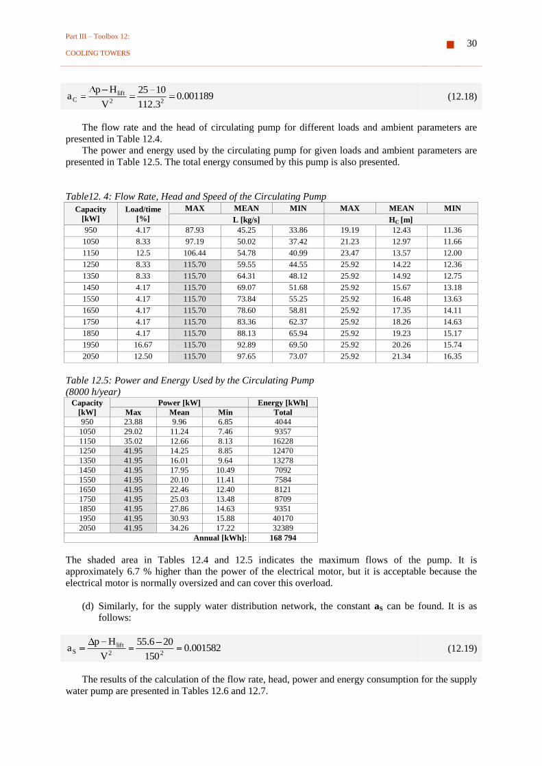
Part III – Toolbox 12:
COOLING TOWERS 30
001189.03.112
1025
V
Hpa
22
liftC (12.18)
The flow rate and the head of circulating pump for different loads and ambient parameters are
presented in Table 12.4.
The power and energy used by the circulating pump for given loads and ambient parameters are
presented in Table 12.5. The total energy consumed by this pump is also presented.
Table12. 4: Flow Rate, Head and Speed of the Circulating Pump
Capacity
[kW]
Load/time
[%]
MAX MEAN MIN MAX MEAN MIN
L [kg/s] HC [m]
950 4.17 87.93 45.25 33.86 19.19 12.43 11.36
1050 8.33 97.19 50.02 37.42 21.23 12.97 11.66
1150 12.5 106.44 54.78 40.99 23.47 13.57 12.00
1250 8.33 115.70 59.55 44.55 25.92 14.22 12.36
1350 8.33 115.70 64.31 48.12 25.92 14.92 12.75
1450 4.17 115.70 69.07 51.68 25.92 15.67 13.18
1550 4.17 115.70 73.84 55.25 25.92 16.48 13.63
1650 4.17 115.70 78.60 58.81 25.92 17.35 14.11
1750 4.17 115.70 83.36 62.37 25.92 18.26 14.63
1850 4.17 115.70 88.13 65.94 25.92 19.23 15.17
1950 16.67 115.70 92.89 69.50 25.92 20.26 15.74
2050 12.50 115.70 97.65 73.07 25.92 21.34 16.35
Table 12.5: Power and Energy Used by the Circulating Pump
(8000 h/year) Capacity
[kW]
Power [kW] Energy [kWh]
Max Mean Min Total
950 23.88 9.96 6.85 4044
1050 29.02 11.24 7.46 9357
1150 35.02 12.66 8.13 16228
1250 41.95 14.25 8.85 12470
1350 41.95 16.01 9.64 13278
1450 41.95 17.95 10.49 7092
1550 41.95 20.10 11.41 7584
1650 41.95 22.46 12.40 8121
1750 41.95 25.03 13.48 8709
1850 41.95 27.86 14.63 9351
1950 41.95 30.93 15.88 40170
2050 41.95 34.26 17.22 32389
Annual [kWh]: 168 794
The shaded area in Tables 12.4 and 12.5 indicates the maximum flows of the pump. It is
approximately 6.7 % higher than the power of the electrical motor, but it is acceptable because the
electrical motor is normally oversized and can cover this overload.
(d) Similarly, for the supply water distribution network, the constant aS can be found. It is as
follows:
001582.0150
206.55
V
Hpa
22
liftS (12.19)
The results of the calculation of the flow rate, head, power and energy consumption for the supply
water pump are presented in Tables 12.6 and 12.7.
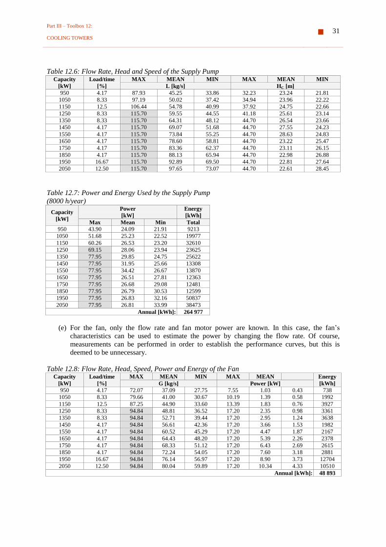
Part III – Toolbox 12:
COOLING TOWERS 31
Table 12.6: Flow Rate, Head and Speed of the Supply Pump Capacity
[kW]
Load/time
[%]
MAX MEAN MIN MAX MEAN MIN
L [kg/s] HC [m]
950 4.17 87.93 45.25 33.86 32.23 23.24 21.81
1050 8.33 97.19 50.02 37.42 34.94 23.96 22.22
1150 12.5 106.44 54.78 40.99 37.92 24.75 22.66
1250 8.33 115.70 59.55 44.55 41.18 25.61 23.14
1350 8.33 115.70 64.31 48.12 44.70 26.54 23.66
1450 4.17 115.70 69.07 51.68 44.70 27.55 24.23
1550 4.17 115.70 73.84 55.25 44.70 28.63 24.83
1650 4.17 115.70 78.60 58.81 44.70 23.22 25.47
1750 4.17 115.70 83.36 62.37 44.70 23.11 26.15
1850 4.17 115.70 88.13 65.94 44.70 22.98 26.88
1950 16.67 115.70 92.89 69.50 44.70 22.81 27.64
2050 12.50 115.70 97.65 73.07 44.70 22.61 28.45
Table 12.7: Power and Energy Used by the Supply Pump
(8000 h/year)
Capacity
[kW]
Power
[kW]
Energy
[kWh]
Max Mean Min Total
950 43.90 24.09 21.91 9213
1050 51.68 25.23 22.52 19977
1150 60.26 26.53 23.20 32610
1250 69.15 28.06 23.94 23625
1350 77.95 29.85 24.75 25622
1450 77.95 31.95 25.66 13308
1550 77.95 34.42 26.67 13870
1650 77.95 26.51 27.81 12363
1750 77.95 26.68 29.08 12481
1850 77.95 26.79 30.53 12599
1950 77.95 26.83 32.16 50837
2050 77.95 26.81 33.99 38473
Annual [kWh]: 264 977
(e) For the fan, only the flow rate and fan motor power are known. In this case, the fan’s
characteristics can be used to estimate the power by changing the flow rate. Of course,
measurements can be performed in order to establish the performance curves, but this is
deemed to be unnecessary.
Table 12.8: Flow Rate, Head, Speed, Power and Energy of the Fan Capacity
[kW]
Load/time
[%]
MAX MEAN MIN MAX MEAN Energy
[kWh] G [kg/s] Power [kW]
950 4.17 72.07 37.09 27.75 7.55 1.03 0.43 738
1050 8.33 79.66 41.00 30.67 10.19 1.39 0.58 1992
1150 12.5 87.25 44.90 33.60 13.39 1.83 0.76 3927
1250 8.33 94.84 48.81 36.52 17.20 2.35 0.98 3361
1350 8.33 94.84 52.71 39.44 17.20 2.95 1.24 3638
1450 4.17 94.84 56.61 42.36 17.20 3.66 1.53 1982
1550 4.17 94.84 60.52 45.29 17.20 4.47 1.87 2167
1650 4.17 94.84 64.43 48.20 17.20 5.39 2.26 2378
1750 4.17 94.84 68.33 51.12 17.20 6.43 2.69 2615
1850 4.17 94.84 72.24 54.05 17.20 7.60 3.18 2881
1950 16.67 94.84 76.14 56.97 17.20 8.90 3.73 12704
2050 12.50 94.84 80.04 59.89 17.20 10.34 4.33 10510
Annual [kWh]: 48 893

Part III – Toolbox 12:
COOLING TOWERS 32
(f) Finally, after installing the new electrical motor and transmission and after implementing the
VSD control system, the electrical energy consumption will be:
[kWh]482,66448,893264,977168,794Enew (12.20)
The expected electrical energy consumption reduction will be:
[%]4.64100240,356,1
240,356,1664,482100
E
EEE
Current
CurrentNew (12.21)
Step 9: Financial Evaluation
(All prices in this chapter can be used only as an illustration. Current prices should be
obtained from the manufacturers)
The unit price of electrical energy is 0.045 c$US/kWh (this price is calculated by taking the total
annual electrical energy cost and dividing it by the total electrical energy consumption). The cost of
electrical energy is then:
year/$US10.030,61240,356,1045.0CECurreent (12.22)
After the implementation of the proposed energy conservation measures the cost of electricity will be
as follows:
year/$US720,21664,482045.0CE New (12.23)
The expected cost reduction for running the cooling system is 39 310 $US/year.
The estimated investment costs are as follows:
DIRECT COSTS (DC)
1. Onsite costs
Purchased-equipment costs (PEC)
– VSD control units for:
Circulating pump (39.33 kW) 6200 $US
Fan of cooling tower (14.7 kW) 3000 $US
Supply pump (115.5 kW) 16 500 $US
– Temperature sensors 500 $US
– Others 2500 $US
Purchased-equipment installation (33 % of PEC) 8500 $US
Piping (5 % of PEC) 1300 $US
Electrical materials (10 % of PEC) 2500 $US
Total onsite costs: 38 500 $US
2. Offsite costs
Civil, structural and architectural work 1500 $US
Service facilities 1000 $US
Total offsite costs: 2500 $US

Part III – Toolbox 12:
COOLING TOWERS 33
TOTAL DIRECT COSTS: 41 000 $US
INDIRECT COST (IC)
Engineering and supervision (8 % of DC) 3200 $US
Construction costs (15 % of DC) 6100 $US
TOTAL INDIRECT COSTS: 9300 $US
TOTAL CAPITAL INVESTMENT (TCI = DC + IC): 47 800 $US
COST-BENEFIT ANALYSIS
years2.139,310
47,800PeriodBack -Pay Simple (12.24)
Notation:
A total area of the wetted surface (includes the
surface area of drops of water as well as the
wetted slates or other fill material), [m2]
a cooling tower approach, [oC]
cp specific heat of fluid at constant pressure
G mass flow rate of air, [kg/s]
h enthalpy, [kJ/kg]
hc convection coefficient, [kW/(m2 K)]
L mass flow rate of water, [kg/s]
M mass flow rate, [kg/s]
NTU number of heat transfer units
r cooling tower range, [oC]
RH Relative humidity of air, [%]
T water temperature, [oC]
t air temperature, [oC]
Q heat capacity of cooling tower, [kW]
CT efficiency of cooling tower, [-]
Subscripts:
w refers to water
a refers to air
db refers to dry bulb
wb refers to wet bulb
in refers to inlet
out refers to outlet
References Arora, C.P. (2000) Refrigeration and Air Conditioning, TataMcGraw-Hill.
Elonka, S.M. (1980) Standard Plant Operators' Manual, McGraw-Hill.
Good Practice Guide No. 225 (1999) Industrial Cooling Water System, Energy Efficiency Office,
Department of the Environment, UK.
Gvozdenac, D., Morvay, Z., Kljajić, M. (2003) Energy Audit of Cooling Towers, PSU-UNS
International Conference 2003: Energy and the Environment, Prince Songkla University, Hat
Yai, Thailand, 11–12 December.
http://myhome.hananet.net/criok (Cooling Tower Technical Site of Daeil Aqua Co., Ltd. for Cooling
Tower Engineers, Operators and Purchaser)
http://www.ctdoc.com (Cooling Tower Doctor)
http://www.marleycoolingtower.com (The Marley Cooling Tower Company)
http://www.chersources.com (Cooling Towers: Design and Operation Considerations)
Kern, D.Q. (1997) Process Heat Transfer, TataMcGraw-Hill.
Perry's Chemical Engineers' Handbook (1997) 7th Edition, McGraw-Hill.
Stoecker, W.F., Jones, J.W. (1984) Refrigeration and Air Conditioning, McGraw-Hill.

Part III – Toolbox 12:
COOLING TOWERS 34