industrial excess heat and district heating: potentials

ECEEE INDUSTRIAL SUMMER STUDY PROCEEDINGS 285

Industrial excess heat and district heating: potentials and costs for the EU-28 on the basis of network analysis

Ali Aydemir Fraunhofer ISIBreslauer Str. 4876139 [email protected]

David Schilling Fraunhofer ISIBreslauer Str. 4876139 KarlsruheGermany

Tobias FleiterFraunhofer ISIBreslauer Str. 4876139 KarlsruheGermany

Mostafa FallahnejadTU WienEnergy Economics GroupGußhausstraße 25–29 1040 ViennaAustria

Keywordswaste heat, district heating

AbstractMany studies see district heating as an important measure to reduce greenhouse gas emissions in the building sector. In this context, industrial excess heat can contribute to the provi-sion of cost-effective heat for district heating networks with a low CO2-footprint. The potential of excess heat to be used for district heating depends, among other things, on the amount of energy available from the supplying factories, the seasonal profiles and the distances to possible district heating areas, which in turn determine possible transport costs for the heat. Here, we present a new method to estimate the costs of sup-plying industrial excess heat to potential district heating areas by calculating potential pipeline connections based on network analysis. As a first step, we map areas with district heating po-tential. In the second step, we calculate how much industrial excess heat can be provided to supply these areas. To do this, we use a database of georeferenced industrial sites containing information on the amount of excess heat (1,058 sites with a total of 94 TWh). In addition, we use a heuristic model to de-sign networks for heat transport between excess heat sources and district heating areas. On this basis, the investments for the necessary infrastructure are estimated. We take into ac-count investments and operating costs for pipelines and heat exchangers as well as heat losses. This results in costs for trans-porting the excess heat to the district heating areas. For our analysis, we vary the parameters in our model and thus gener-ate cost-potential curves to show how much excess heat can be transported to the district heating areas at which costs. For the

EU-28, our calculation shows that about 34 TWh of excess heat could be provided for transport costs of up to 0.75 ct./kWh. This corresponds to about 36 % of the excess heat in the data set. A further 13 % can be provided at costs of up to 1.5 ct/kWh. In total, about 54 % of the excess heat can be provided for costs of up to 2 ct./kWh.

IntroductionAbout 70 % of energy consumption in industry is due to the provision of process heat, resulting in large amounts of unused excess heat. From a technical point of view, excess heat can be described as unwanted heat generated by an industrial process (Pehnt 2010). From a social point of view, it can be described as heat which is a by-product of industrial processes and currently not utilized, but which could be used for society and industry in the future (Broberg Viklund and Johansson 2014).

Industrial excess heat is generated by inefficiencies of plants and processes as well as by thermodynamic constraints (cf. Hirzel 2013, Johnson et al. 2008). One example of plant inef-ficiencies is the lack of insulation to reduce heat losses. Ther-modynamic limitations, on the other hand, result from pro-cess characteristics. One example is the melting of aluminium in flame furnaces. Exhaust gases leaving the furnace can reach temperatures of up to 1,300 °C. As a result, the waste gases contain a high heat content, which accounts for up to 60 % of the energy input of the furnace. An energy efficiency meas-ure for flame furnaces would therefore be to strive for lower exhaust gas temperatures, e.g. through better heat transfer in the furnace. But even in this case, the laws of thermodynam-ics prescribe a lower limit for the exhaust gas temperature.

REVISED 30 SEPTEMBER 2020

4-073-20 AYDEMIR ET AL

286 INDUSTRIAL EFFICIENCY 2020

4. TECHNOLOGY, PROCESSES AND SYSTEMS

During heat exchange in the furnace, energy is transferred from a high temperature source to a low temperature sink. To achieve melting of the aluminium, the combustion gas temperature must always be above the melting point for alu-minium, otherwise no melt is produced. The melting point of aluminium is between 650 and 750 °C, consequently the low-er limit for the exhaust gas temperature is also in this range. In relation to the energy input in the furnace, at an exhaust gas temperature in this range at least 40 % of the energy fed into the furnace would still be lost as excess heat. The type of kiln and the function therefore specifies a minimal amount of excess heat in the exhaust gas due to thermodynamic restric-tions. However, this excess heat could be made available to other processes and the unused industrial excess heat would thus be reduced overall.

In Europe, industrial excess heat utilisation is not new. For example, Bergmeier (2003) summarizes the history of waste energy recovery in Germany, starting in 1920’s. Already in the 1920’s, numerous journals dealt with the topic of “heat manage-ment” and in this context measures to increase energy efficien-cy by using industrial excess heat were discussed. Bergmeier (2003) concludes that in the past, fewer technical barriers were decisive for the wider use of excess heat. Rather, the barriers were always economic, social and political barriers that stood in the way of a broader use.

Excess heat in the context of district heatingFor the use of industrial excess heat, different measures can be weighed up against each other in terms of economic efficien-cy and environmental friendliness. In engineering practice, a staged approach is used, which prioritises the different possi-bilities as shown below:

1. Avoiding the generation of excess heat.

2. In-process use of excess heat (by heat transfer).

3. Factory-internal use of excess heat (by heat transfer).

4. Conversion of excess heat into other media (e.g. electric-ity, cooling, compressed air), or factory-external use of the excess heat.

Case studies, completed projects and scientific contributions indicate that even after carrying out steps 1 to 3, considerable amounts of excess heat would remain. These amounts of heat could then be used for external supply. Aydemir and Rohde (2018), for example, analyse the potential for heat integration in German industry. Heat integration is an umbrella term for concepts for the thermal combination of stationary or discon-tinuous processes for the purpose of heat recovery through heat transfer (cf. Klemeš and Kravanja (2013)).With regard to the staged approach mentioned above, it is therefore the sys-tematic elaboration of steps 1 to 3. To estimate the potential, Aydemir and Rohde (2018) use a step-by-step approach, with which they attempt to quantify the effect of a cascade-like pro-cess control of heat supply. As a result, a theoretical potential for heat integration of about 10–11 %, based on the final energy consumption of industry, is quantified. About 30 to about 50 % (depending on the scenario) are due to external heat integra-tion, i.e. the external use of excess heat. This heat can be used

either to provide heat for other production plants (cf. Aydemir et al. (2017)) or for district heating networks.

Another example is the contribution of Persson et al. (2014) by estimating the potential contribution of industrial excess heat to the heating of buildings for the EU-28. For this purpose, the European Pollutant Emission Register is used to estimate how much excess heat is generated by industrial plants, how much of it is used within the plants and how much excess heat could thus be provided externally for district heating networks. In addition, numerous projects have already been carried out in the past in which industrial excess heat has been integrated as an energy source for district heating networks, or correspond-ing projects are being planned (cf. Petersen&Energie (2017)).

Overall, industrial excess heat is therefore considered as a promising energy source for district heating networks, which might be on the one hand cheap and on the other hand can lead to overall greenhouse gas reductions, at least in the context of a transition phase towards a greenhouse gas neutral economy (cf. Buehler et al. (2018)). In this context, however, few analyses have been carried out to date that assess the potential for using industrial excess heat in district heating networks for the entire EU on a site-specific basis, taking into account the necessary infrastructure and corresponding costs.

Here, we present a new method to estimate the costs of sup-plying industrial excess heat to potential district heating areas by calculating potential pipeline connections based on network analysis. The method contains individual locations of heat sources and sinks, the potential pipeline connection between points and seasonal variations in both the supply and the de-mand profiles. We apply the method to an open data set con-taining industrial sites and heat demand densities for the EU-28 countries. We calculate cost-potential curves for the transport of excess heat from industrial sites to potential district heating clusters. Both, the method and the data are available as open source online tool (https://www.hotmaps.hevs.ch/map).

Data and methodology

DATAThe analysis builds on the following two major data-sets. Both are publicly available as open data.

• Heat demand buildings: To identify areas with promising properties for district heating networks, a map for the heat demand density of buildings is used. This map shows the estimated energy demand of buildings for space heating and hot water. The data are available in spatial resolution in the form of digital raster maps with a resolution of 100 by 100 metres and cover the EU-28. The estimation of energy demand is based, among other things, on population data, regionally differentiated building stock characteristics and locally differentiated heating degree days. The methodology is described in detail in Pezutto et al. (2018) and Müller et al. (2019). The data set is publicly available for download.1

1. Industrial plants: https://gitlab.com/hotmaps/industrial_sites/industrial_sites_Industrial_Database.




• Excess heat from industrial sites: For excess heat from industrial sites, a data set from Manz et al. (2018) was used. The data set estimates the industrial excess heat for 1,058 sites in the EU-28, in total about 94 TWh. The indus-trial sites are located by coordinates. The data set is based on data from the EU Emissions Trading Scheme (ETS data) and production statistics. In the ETS data, CO2 emissions are shown for individual production sites, differentiated by industry and year (e.g. for the cement and lime production industry). The production statistics show national produc-tion quantities for certain products (e.g. national cement production in a certain year). The data set has been cre-ated in two basic steps. In the first step, based on national production statistics and the assigned CO2 emissions in the ETS data, production volumes for specific products are es-timated for the production sites listed in the ETS data. For this purpose, the following data are put in relation to each other: total allocated CO2 emissions per industry and coun-try, total production of a specific product per industry and country, and allocated CO2 emissions per site. In principle, a specific CO2 emission factor (CO2/tonne of product) is formed for the national level for this estimation in order to estimate the production volumes for the sites under consid-eration. In the second step, the production quantities per site are assigned to a certain production process in order to allow a specific estimate of the excess heat potentials. In a third step, specific excess heat potentials from literature (in e.g. GJ/tonne of glass produced) are then related to each process. Here, we can consider specific differences across processes, whereas we assume there are not differences in the specific excess heat across countries for a single process. In the fourth step, the total available excess heat is calculated by multiplication with the total production quantity per site. The methodology is explained in more detail in Manz et al (2018). The data set is publicly available for download.2

METHODOLOGYThe methodology for the assessment of integration potentials for excess heat in district heating networks is based on two steps. As a first step, we map areas with district heating poten-tial. In the second step, we calculate how much industrial ex-cess heat can be provided to supply these areas and at what cost. For the second step we use a network algorithm. This has the following background: if there are only few sources of excess heat, one single pipeline per source could always be consid-ered for transporting the heat to a nearby area with favourable conditions for district heating. However, if several excess heat sources are to flow into one and the same area, it would make sense to collect the heat and transport it to the area in a larg-er common pipeline. The approach with one pipe per source would thus tend to overestimate the cost of the pipelines. To counteract this, the pipeline planning problem was approxi-mated by assuming a network flow problem. To solve the prob-lem, a heuristic model is used in which the excess heat can be bundled and transported to the potential users. The two steps are explained in more detail below.

2. Heat density maps: https://gitlab.com/hotmaps/building_footprint_tot_curr.

Step 1: mapping areas with district heating potentialFor this step we use the map for the heat demand density of buildings (abbreviated heat map). A common approach is to identify areas with potential for district heating based on heat demand densities (energy demand per area). Above a defined minimum heat demand density, the area has district heating potential. The minimum heat demand densities to be defined are based either on empirical values or techno-economic con-siderations.

We implement this in our model in two steps. In the first step, all the cells of the heat map with heating demand below the minimum heat demand density are filtered and eliminated. By eliminating these cells from the map, we obtain groups of cells that are attached to each other (polygons). Each set of these attached cells constitutes a zone. In the second steps, the total heat demand in each of the zones is calculated. For a zone, if the total heat demand is higher than the minimum heat de-mand density, then, it is considered as potential district heat-ing area. We define the minimum heat demand density in our model based on Persson et al. (2017), it is 50 TJ/km².

To use the network algorithm it is necessary to generate feed-in points within the zones. These are points up to which fictitious pipelines can be drawn for the supply of industrial excess heat. We do this by adding equidistant entry points to each zone.

Step 2: Generation of networks to transport excess heatIn the second step, we calculate how much industrial excess heat can be provided to supply the zones identified in step 1. To do this, we use the database of georeferenced industrial sites containing information on the amount of excess heat available and the temperature. Only sources with a temperature above 100 °C are included in the analysis, since the temperature for the flow of the heating network is assumed to be 100 °C. In addition, we use a self-developed heuristic model to design net-works for heat transport between excess heat sources and dis-trict heating areas. The heuristic is based on five interim steps.

In the first interim step, all points within a considered area that do not exceed a maximum distance are connected. Thus, excess heat sources (in the following only sources) are con-nected to sinks, sources to sources and sinks to sinks. Then we cut out an area where all considered points do not exceed a defined minimum distance. In our analysis it is 50 kilometres. The maximum distance serves most of all to reduce the com-putational effort. If a too small maximum distance is selected, many interesting networks may not be found. If the distance is chosen too high, the computing time is increased unnecessar-ily, because waste heat feeds become unrealistic from a certain distance on.

The distance of the connections between the points are then used in the second interim step as so-called edge weights. A minimum spanning tree is computed with the distance of the edges as weights. Thus the distances within the network are re-duced to the minimum, with the boundary condition that all points are still at least indirectly connected to each other (cf. Figure 1). At this point, the network is defined, but the actual heat flows are not yet considered.

In the third interim step the maximum possible heat trans-port is calculated for each network. This takes into account that several sinks can be connected in one network and the heat




flow is reduced by each sink. In addition, the weekly load pro-file of possible relationships between sources and sinks is taken into account. The annual load profiles are aggregated to weeks over one year in order to consider seasonal changes in demand and supply. A higher resolution to e.g. daily profiles would also be possible, but would have increased the required computing performance substantially.

To find the maximum flow between source and sink (over the course of the year), the load profiles of the considered combination of source and sink are intersected. For each week considered, the value that is lower is then chosen to determine the maximum power flow for the combination (cf. Figure 2). In the left-hand example in Figure 2, the power of the heat source (i.e. the excess heat) would be consistently lower than the power of the heat sink. In the middle example, the power of the heat source would be partly higher and partly lower than the power of the heat sink. In our model, we want to use as much excess heat as possible, so in both cases the design of the components would refer to the power of the heat source.

In the example on the right, the power of the heat source is consistently higher than that of the heat sink. In this case, therefore, the maximum power of the heat sink would be used to design the system.

In the fourth interim step, the necessary investments and operating costs for connecting the points in the network are esti-mated and heat losses are considered. The edges represent pipe-lines. First, a diameter for the pipes per edge is selected based on the maximum power along the edges. For this purpose, relation-ships between the power to be transported and the associated usual nominal diameters from Nielsen et al. (2013) are used. Based on this, the investment for the pipelines is calculated ac-cording to the distances in the network per edge (using cost data for pipes per meter from Nielsen et al. (2013)). In addition, the pumping needs (PN) based on the pressure loss of the pipelines per edge is calculated according to equation 1. In this equation PL stands for the pressure drop and V for the water volume flow in the pipes; both are based on values given in a Swedish cost catalogue for district heating pipes with optimum flow velocities. (cf. Swedish District Heating Association et al. (2007)). ηpump is the efficiency of the pump, which we assume to be 80 %.

PN = (PL· V) ÷ (ηpump) (1)

The investment required for pumps (Ipump) is calculated on the basis of equation 2. Pmax is the maximum rated power that the pump must deliver when maximum heat is transported (cf. Fig-ure 2). CF is the cost factor based on Danish Energy Agency (2017).

Ipump = Pmax · CFpump, with (2)

CFpump = 240k euro/MW if Pmax < 1 MW, or CFpump = 90k euro/MW else

Furthermore, the heat loss for the pipelines is calculated ac-cording to Equation 3. In this equation, L is the pipe length, HI is the insulator conductivity, Th the temperature of the water in the pipe, Ts the temperature outside the pipes, which is approxi-mated with the soil temperature, IT is the insulation thickness and HD the pipe’s hydraulic diameter. The parameters for the variables are taken from a Swedish cost catalogue for district heating pipes based on the nominal diameter for the pipes, i.e. for the insulation thickness standard values based on the diameters for the pipes are used (cf. Swedish District Heating Association et al. (2007)).

1

2 3

1 1

3 5 6

9Area 1

Area ...n

1

2

1 1

3

9Area 1

Area ...n

Minimum spanning tree

Figure 1. Visualisation of steps 1 and 2: Calculation of the minimum spanning tree between all points. Red represents heat sinks, blue heat sources.

Pmax Pmax Pmax

Power P P

week week week

Figure 2. Visualisation for the intersection of load profiles; blue is for the sink, red for the source.




HL =(L · 10-6 · 2π · HI · (Th - Ts))÷(ln(1 + 2 · IT ÷ HD)) (3)

In addition, the investments for heat exchangers per source and sink are calculated according to the maximum capacity. For the source side air to liquid heat exchangers are assumed using Equation 4. For the sink side liquid to liquid heat exchangers are assumed using equation 5 (cf. Swedish District Heating As-sociation et al. (2007)). In the equation Pmax is the maximum heat transport for the pipe under consideration (cf. Figure 2).

Iheat exchanger source = Pmax · CFheat exchanger source, with (4)

CFheat exchanger source = 15k euro/MW

Iheat exchanger sink = Pmax · CFheat exchanger sink, with (5)

CFheat exchanger sink = 265k euro/MW if Pmax < 1 MW, or CFpump = 100k euro/MW else

Based on the previous calculations, a ratio of costs to heat transport (CH) is defined for each pipe according to equa-tion 6. IPipe and IPump are investments. CRF is the discount fac-tor for taking into account the cost of capital (cf. equation 7). CO&M includes the costs of operating a pump corresponding to the calculated pumping needs from equation (1) and electricity costs for industrial users per EU country from Eurostat (2018). Furthermore, maintenance costs, which are assumed to be one percent of the investment sum are included in CO&M. EH is the used excess heat flowing through the considered pipe and HL are the heat losses reducing the transported excess heat in this pipe. Please note that the factor CH does not include the costs for heat exchangers.

CH = (CRF · (Ipipe + Ipump) + CO&M ) (6)

÷ (EHin pipe - HLin pipe), with

CRF = (i · (1 + i)n) ÷ ((1 + i)n – 1) (7)

In the fifth interim step, we use CH to optimize the design of the network. For this purpose, a maximum ratio of cost to heat transport (CHmax) per pipeline is first defined. For the variation, all pipes that exceed this maximum ratio are then re-moved. Since the flow in the network is then interrupted, a new network is generated based on the previous steps 2 and 3. This is repeated iteratively until CH falls for all pipelines in the net-work below CHmax. Basically the following relationships apply: the higher the CHmax, the more industrial excess heat is trans-ported in the network. However, a higher CHmax also means higher investments and costs for the network and thus has an impact on the costs of heat transport in the network.

Finally, the costs of transporting industrial excess heat per network are calculated using Equation 8. This equation in-cludes the costs for all components of the final total network (i.e. all pipelines, pumps and heat exchangers) and these are set in relation to the delivered excess heat. We call this the levelised cost of heat (LCOH) of the respective network.

LCOH = (CRF· (Iall pipes + Iall pumps + Iall heat exchangers) (8)

+ CO&M) ÷ (EHdelivered in complete network - HLin complete network)

The factor CHmax thus determines how much heat is transport-ed in the networks at what cost and thus also effects the result-ing LCOH per network. Therefore, by varying the CHmax factor

we can develop cost-potential curves for the heat transport. An example network for the province Hainaut in Belgium is shown in Figure 3.

Results: Case study for EU-28 excess heat potentialsFigure 4 shows the amount of excess heat delivered for the countries investigated as a function of the LCOH for the net-works in the form of cost-potential curves. For all countries together, up to LCOH of 0.75 ct./kWh about 34 TWh of excess heat is delivered, which corresponds to 36 % of the total excess heat in the data set. For an LCOH of up to 1.5 ct./kWh, 46 TWh of excess heat are delivered, which corresponds to about 49 % of the amount in the data set; up to 2.0 ct./kWh 6.5 TWh are add-ed, so that in total 51 TWh are delivered, which corresponds to 54 %. From this point on, the increase decreases strongly with increasing LCOH, up to 5 ct./kWh only 2.3 TWh are added, so that in total 53 TWh are delivered, which corresponds to a share of about 57 %. After that, no additional excess heat is delivered, because in our model the heat losses would exceed the possible supply quantities.

With regard to the share of countries in relation to the total excess heat delivered, two countries dominate in the analysis. With an LCOH of 0.75 ct./kWh, Germany and Italy have a share of 45 % of the total excess heat supplied (Germany: 26 %, Italy: 19 %). This trend continues even with higher LCOH, with an LCOH of 1.5 ct./kWh these two countries still have a share of 38 %. This indicates that in these two countries there are many excess heat sources close to residential areas with district heating potential that could be tapped relatively cheaply. The second group of countries with rather high shares of the total excess heat delivered are France, Spain, Belgium and the UK, with shares of 7–9 % at an LCOH of 1.5 ct./kWh.

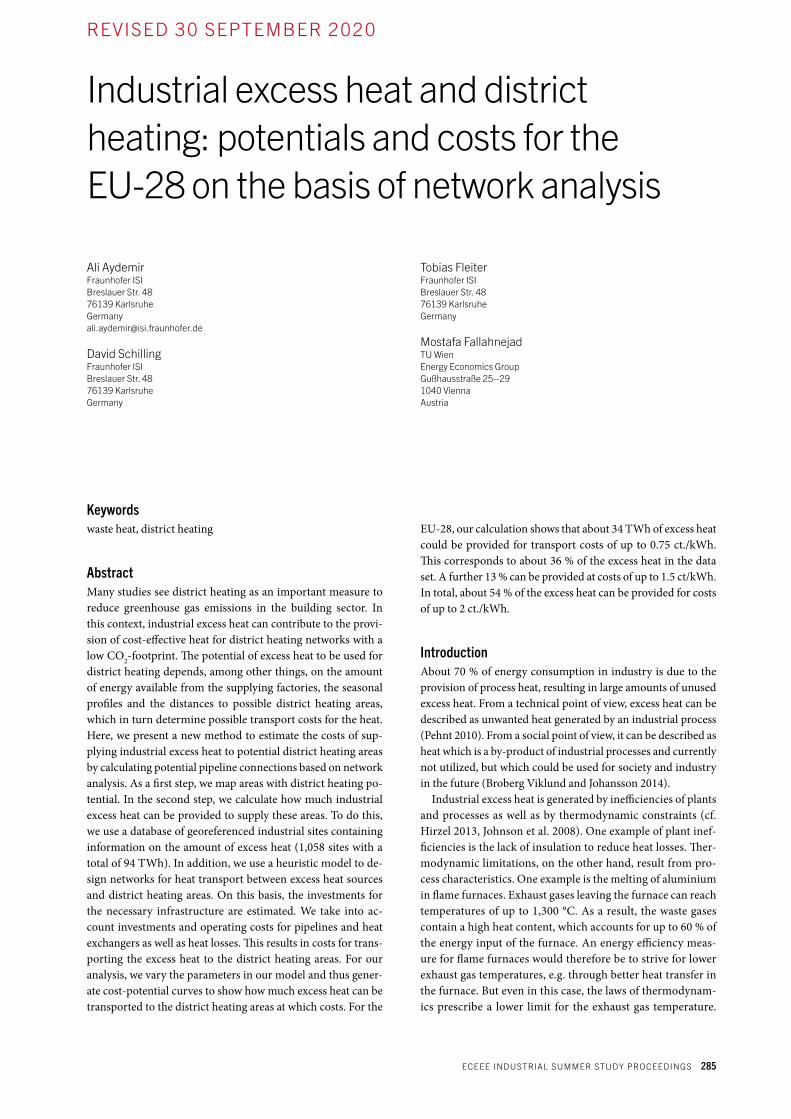
Figure 5 shows the delivered excess heat differentiated for the investigated countries in a map. The picture described above; Germany and Italy supply comparatively large amounts of ex-cess heat, is reflected in the map. In addition, it can be seen that with increasing LCOH more excess heat is delivered, e.g. the interval for France and Portugal changes when the LCOH rises from up to 0.75 ct./kWh to up to 1.5 ct./kWh.

Figure 6 shows the delivered excess heat in relation to the available excess heat per country. It can be seen that even at an

Figure 3. Exemplary network generated based on the described

method.




LCOH of up to 0.75 ct./kWh, more than 80 % of the available excess heat in Denmark and more than 60 % of the available excess heat in the Netherlands is delivered. With an LCOH of up to 1.5 ct/kWh, more than 60 % of the excess heat is also de-livered in Austria, Belgium, Germany and Finland.

DiscussionIn this paper the potential of industrial excess heat for district heating networks is investigated. For this purpose, among other things, a database for industrial sites is used, which estimates the externally available excess heat potential of the sites under consideration on the basis of literature data and public data. However, it should be emphasised that it is not always com-pletely clear from the literature figures used to what extent in-ternal heat utilisation possibilities have been taken into account in the figures. The more consistently internal utilisation possi-bilities are exploited, the lower the potential for external provi-sion and thus the potential of industrial excess heat for district heating. There is therefore still a need for research in this area to quantify the potential. This is particularly important against the background of a possible change in the provision of process heat in the future, with the aim of decarbonising it. In this con-text heat pumps powered by renewable electricity are discussed as a promising option. In order to increase the efficiency of heat

pumps in industry, the use of excess heat is essential. In such a scenario, this could well lead to the fact that at many industrial sites significantly more excess heat could be used internally and thus less excess heat would be left for external supply.

The industrial excess heat included in the data set used is relatively low compared to other estimates of industrial excess heat for the EU-28. For example, Persson et al. (2014) estimated a potential of 398 TWh of industrial excess heat for the EU-27, which is about four times higher than the sum in our data set. One reason is that Persson et al. (2014) have recorded more production sites compared to Manz et al. (2018). However, the excess heat is not estimated on the basis of technical processes, but rather simplified on the basis of characteristic values. Pa-papetrou et al. (2018) estimate an industrial excess heat po-tential of 304 TWh for the EU. However, they use a top-down approach, so no estimation is made for individual production sites. Our analysis therefore only refers to a fraction of the available excess heat. This means that this analysis cannot yet show what proportion of the total industrial excess heat within the EU-28 could be used for heat supply at what cost. Therefore, the relative results of the analysis are of particular interest: what percentage of the excess heat from the data set is provided at what cost.

With regard to the method, it should be noted that although distances are taken into account, local conditions are not. For

Figure 4. Cost-potential curves: Excess heat delivered as a function of LCOH.




LCOH ≤ 0.75 ct./kWh



Excess heat delivered per

country for different

LCOH

Figure 5. Excess heat delivered per country for different LCOH.







Excess heat delivered

in % of available heat in

dataset per country for

different LCOH

Figure 6. Excess heat delivered in % of available heat in dataset per country for different LCOH.




Bühler, F., Petrović, S., Holm, F. M., Karlsson, K., & Elmeg-aard, B. (2018). Spatiotemporal and economic analysis of industrial excess heat as a resource for district heat-ing. Energy, 151, 715–728. https://doi.org/10.1016/j.energy.2018.03.059.

Danish Energy Agency and Energinet. (2017). Technology data for Energy Transport. https://ens.dk/sites/ens.dk/files/Analyser/technology_data_for_energy_transport_dec_2017_1.pdf.

eurostat. Electricity prices for non-household consumers – bi-annual data (from 2007 onwards): for 2018. https://ec.europa.eu/eurostat/statistics-explained/index.php/Electricity_price_statistics#Electricity_prices_for_non-household_consumers.

Johnson, I., William, T., Choate, W. T., & Amber Davidson, A. (2008). Waste heat recovery: technology and opportuni-ties in US industry. http://www1.eere.energy.gov/manu-facturing/intensiveprocesses/pdfs/waste_heat_recovery.pdf. Accessed 26 April 2016.

Klemeš, J. J., & Kravanja, Z. (2013). Forty years of Heat Inte-gration: Pinch Analysis (PA) and Mathematical Program-ming (MP). Current Opinion in Chemical Engineering, 2, 461–474. https://doi.org/10.1016/j.coche.2013.10.003.

Manz, P., Fleiter, T., & Aydemir, A. (2018). Developing a geo-referenced database of energy-intensive industry plants for estimation of excess heat potentials. eceee Industrial Summer Study Proceedings, 2018.

Müller, A., Hummel, M., Kranzl, L., Fallahnejad, M., & Büchele, R. (2019). Open Source Data for Gross Floor Area and Heat Demand Density on the Hectare Level for EU 28. Energies, 12, 4789. https://doi.org/10.3390/en12244789.

Nielsen, S., & Möller, B. (2013). GIS based analysis of future district heating potential in Denmark. Energy, 57, 458–468. https://doi.org/10.1016/j.energy.2013.05.041.

Papapetrou, M., Kosmadakis, G., Cipollina, A., La Commare, U., & Micale, G. (2018). Industrial waste heat: Estimation of the technically available resource in the EU per indus-trial sector, temperature level and country. Applied Ther-mal Engineering, 138, 207–216. https://doi.org/10.1016/j.applthermaleng.2018.04.043.

Pehnt, M. (2010). Energieeffizienz: Ein Lehr- und Handbuch. Berlin, Heidelberg: Springer-Verlag Berlin Heidelberg.

Persson, U., Möller, B., & Werner, S. (2014). Heat Road-map Europe: Identifying strategic heat synergy regions. Energy Policy, 74, 663–681. https://doi.org/10.1016/j.enpol.2014.07.015.

Persson, U., Möller, B., & Wiechers, E. (2017). Methodologies and assumptions used in the mapping: Deliverable 2.3: A final report outlining the methodology and assumptions used in the mapping: Heat Roadmap Europe. https://heatroadmap.eu/wp-content/uploads/2018/11/D2.3_Re-vised-version_180928.pdf.

Petersen, A. B., & Energi, G. (2017). Handbook: 25 cases of urban waste heat recovery. https://www.reuseheat.eu/wp-content/uploads/2018/03/6.1-Other-experiences-25-case-studies.pdf. Accessed 13 March 2020.

Pezzutto, S., Zambotti, S., Croce, S., Zambelli, P., Garegnani, G., Scaramuzzino, C., et al. (2018). D2. 3 WP2 Report – Open Data Set for the EU28. Wien: Technische Universität

example, the course of roads or existing buildings can signifi-cantly change the cost of laying district heating pipes. Further developments are necessary at this point. For example, by using GIS systems to take greater account of local conditions when calculating costs.

Finally, it should be stressed that the analysis examines the potential for using industrial excess heat in areas with prom-ising characteristics for district heating. This does not mean, of course, that district heating networks must already exist in these areas. At this point, therefore, an analysis that takes into account the real distribution of existing district heating net-works in Europe would be desirable.

ConclusionIn the present analysis, we develop a method to generically calculate transport costs for feeding industrial excess heat into potential district heating areas. We apply the method to data containing excess heat potentials from 1,058 industrial sites in Europe. We find that about 50 % of the excess heat could be pro-vided at transport costs of up to 1.5 ct./kWh. This includes in-frastructure investments as well as operating and maintenance costs. In addition, the load profile of the heat suppliers and the possible heat consumers is taken into account when matching heat sources and sinks. The method and the open data set allow similar assessments for selected regions and countries.

All in all, the calculated potentials and their transport costs indicate that industrial excess heat is an attractive energy source for district heating networks and can contribute to de-carbonise district heating grids at low costs. However, it has to be underlined that many of the calculated excess heat po-tentials first require the built-up of district heating infrastruc-ture. The connection of excess heat sources can be a driver to establish a local district heating infrastructure (cf. Popovski et al. (2019)). Nevertheless, the question has to be addressed to what extent this will remain so in the future against the background of a changing industry. Of particular interest here is how a possible decarbonisation of the supply of industrial process heat will change the supply of industrial excess heat quantitatively and qualitatively; and to what extent this will affect the possible role of industrial excess heat for district heating networks.

References Aydemir, A., Ko, D., & Rohde, C. (2016). Energy savings of

inter-company heat integration: Tapping potentials with spatial analysis. eceee Industrial Summer Study Proceed-ings, 2016.

Aydemir, A., & Rohde, C. (2018). What about heat integra-tion? Quantifying energy saving potentials for Germany. eceee Industrial Summer Study Proceedings, 2018.

Bergmeier, M. (2003). The history of waste energy recovery in Germany since 1920. Energy, 28, 1359–1374. https://doi.org/10.1016/S0360-5442(03)00114-2.

Broberg Viklund, S., & Johansson, M. T. (2014). Technolo-gies for utilization of industrial excess heat: Potentials for energy recovery and CO2 emission reduction. Energy Conversion and Management, 77, 369–379. https://doi.org/10.1016/j.enconman.2013.09.052.




Swedish District Heating Association et al. (2007). Kulvertko-stnadskatalog (The district heating pipe cost catalogue). www.energiforetagen.se/globalassets/energiforetagen/det-erbjuder-vi/publikationer/kulvertkostnadskata-log_2007-1.pdf.

AcknowledgementsThis paper is based on work packages carried out within the project Hotmaps. This project has received funding from the European Union’s Horizon 2020 research and innovation pro-gramme under grant agreement No 723677.

Wien-Institute of Energy Systems and Electrical Drives-Energy Economics Group.

Popovski, E., Fleiter, T., Santos, H., Leal, V., & Fernandes, E. O. (2018). Technical and economic feasibility of sustain-able heating and cooling supply options in southern European municipalities – A case study for Matosinhos, Portugal. Energy, 153, 311–323. https://doi.org/10.1016/j.energy.2018.04.036.

Sächsische Energieagentur GmbH (SAENA). (2012). Tech-nologien zur Abwärmenutzung. http://www.saena.de/download/Broschueren/BU_Technologien_der_Abwaer-menutzung.pdf. Accessed 27 January 2016.

industrial excess heat and district heating: potentials

Documents