industry tournament incentives and the strategic value of
TRANSCRIPT

Industry Tournament Incentives and the Strategic Value of Corporate Liquidity
Jian Huanga, Bharat A. Jain
a, Omesh Kini
b, *
a College of Business and Economics, Towson University, Towson, MD 21252 b Robinson College of Business, Georgia State University, Atlanta, GA 30303
First draft: February 2014
Latest draft: September 2015
_____________________________________________________________________________________
Abstract
We evaluate the link between CEO industry tournament incentives (ITI) and the strategic value of
corporate liquidity. We find that ITI increase the level and marginal value of cash holdings even after
conducting several tests to control for endogeneity. Additionally, for firms with excess cash, higher ITI
lead to increased R&D expenditures and spending on focused acquisitions, and reduced shareholder
payouts. Furthermore, ITI strengthen the relation between firm cash holdings and market share gains.
Overall, our results suggest that ITI increase the value of cash by incentivizing CEOs to deploy cash
strategically to capture its product market benefits.
JEL classification: G31; G32; G34; J31; J33; L25; D21
Keywords: Industry tournament incentives; Marginal value of cash; Level of cash; Dissipation and
accumulation of excess cash; Strategic investments; Market share; Product markets
_____________________________________________________________________________________
☆We would like to thank Naveen Daniel, Jarrad Harford, and Amiyatosh Purnanandam for helpful
comments. We thank Ryan Williams for his help with the construction of some of our incentive related
variables. The usual disclaimer applies.
*Corresponding author. Robinson College of Business, Georgia State University, Atlanta, GA 30303,
USA. Tel. + 1-404-413-7343; Fax: + 1-404-413-7312.
E-mail addresses: [email protected] (Jian Huang), [email protected] (Bharat A. Jain), [email protected]
(Omesh Kini).

Industry Tournament Incentives and the Strategic Value of Corporate Liquidity
_____________________________________________________________________________________
Abstract
We evaluate the link between CEO industry tournament incentives (ITI) and the strategic value of
corporate liquidity. We find that ITI increase the level and marginal value of cash holdings even after
conducting several tests to control for endogeneity. Additionally, for firms with excess cash, higher ITI
lead to increased R&D expenditures and spending on focused acquisitions, and reduced shareholder
payouts. Furthermore, ITI strengthen the relation between firm cash holdings and market share gains.
Overall, our results suggest that ITI increase the value of cash by incentivizing CEOs to deploy cash
strategically to capture its product market benefits.
JEL classification: G31; G32; G34; J31; J33; L25; D21
Keywords: Industry tournament incentives; Marginal value of cash; Dissipation and accumulation of
excess cash; Strategic investments; Market share; Product markets
_____________________________________________________________________________________

1
1. Introduction
Recent research suggests that the inherent optionality present in industry and intra-firm
tournaments provide managers with distinct and incremental career enhancing incentives from option-
based compensation schemes to implement riskier but value enhancing firm policies (Coles, Li, and
Wang, 2013; Kale, Reis, and Venkateswaran, 2009; and Kini and Williams, 2012). For example, focusing
on intra-firm tournaments that arise as a result of the compensation gap between the CEO and top
managers, Kale, Reis, and Venkateswaran (2009) find that the option-like feature of winning the CEO
promotion tournament within the firm positively influences firm performance, while Kini and Williams
(2012) document that it also encourages firm risk taking. Extending the notion of tournaments beyond the
top management team to focus on the CEO, Coles, Li, and Wang (2013) find that CEO industry
tournament incentives, as captured by the compensation gap between the firm’s CEO and higher paid
CEOs operating in the same product market (for example, the pay differential between the firm’s CEO
and the maximal industry CEO pay), encourage the adoption of riskier but value enhancing corporate
policies.
Corporate liquidity decisions are especially vulnerable to potential agency conflicts between
managers and shareholders because it is not easy to ascertain whether managerial actions with regard to
the accumulation, maintenance, and dissipation of cash are driven by managerial self-interest or
shareholder interest (see, e.g., Harford, 1999; Dittmar and Mahrt-Smith, 2007; and Harford, Mansi, and
Maxwell, 2008). Nalebuff and Stiglitz (1983) and Zabojnik and Bernhardt (2001) suggest that
tournaments are particularly valuable when extracting managerial effort from output signals is difficult.
Thus, tournament incentives can potentially serve as economically efficient mechanisms to induce
managers to pursue cash policies that are consistent with shareholder value maximization. To shed light
on this issue, we empirically examine the impact of CEO industry tournament incentives (henceforth
referred to as ITI) on the: (i) marginal value of corporate cash holdings, (ii) level of cash holdings, (iii)
rate of accumulation and dissipation of excess cash, and (iv) strategic actions that entail the use of excess

2
cash to obtain competitive benefits in the firm’s product markets. We focus on ITI primarily because,
amongst all the senior managers, the CEO is likely to have the most influence on the cash policies of the
firm due to the importance of cash as a “strategic” resource (see, e.g., Benoit, 1984; Bolton and
Scharfstein, 1990; Campello, 2006; and Fresard, 2010). While our emphasis is on CEO industry
tournament incentives, we control for intra-firm tournament incentives as well as the CEO’s shareholder
alignment of interest (CEO delta) and risk-taking (CEO vega) incentives that arise from her compensation
structure in all our empirical tests.
Our focus on examining how ITI shape various facets of firm cash policy and their economic
consequences is also driven by the growing propensity for U.S. corporations to stockpile huge cash
reserves well in excess of what is required to fund operations coupled with the dramatic and secular
increase in their cash holdings.1 The overarching concern with regard to greater managerial access to
liquidity arises from cash being a fundamentally different type of asset in the hands of management,
largely because of the flexibility it provides them in terms of decisions related to its accumulation and
dissipation. The pursuit of managerial self-interest can result in the unproductive utilization of cash
holdings as a result of either overinvestment or underinvestment. In the former case, cash enables
managers to pursue risky empire building investments that can destroy shareholder value but increase
their personal benefits (Jensen, 1986). In the latter case, a combination of managerial risk aversion and
preference for the "quiet life" (Bertrand and Mullainathan, 2003) can result in shareholder wealth
destruction due to underinvestment of cash holdings.2
While the discretionary nature of cash holdings can impose substantial costs on shareholders as
described above, it also has the potential to generate considerable strategic and hedging benefits. For
1 Gao, Harford, and Li (2013) report that cash represents approximately 20.45% of firm assets as of 2011. In
addition, Bates, Kahle, and Stulz (2009) report that the average cash ratio for U.S. firms has doubled during the
1980 – 2006 period. 2 In support of the notion that agency conflicts negate any potential benefits of liquidity, Faulkender and Wang
(2006) find that shareholders of an average firm assign a value of $0.94 for each dollar of cash in the hands of
management. Similarly, Nikolov and Whited (2014) estimate that typical agency problems can result in increased
cash holdings and a significant drop in shareholder value.
3
instance, Fresard (2010) points out that cash holdings have a strategic dimension that can affect firm and
rival product market strategies and outcomes. Specifically, research suggests that there are at least three
avenues through which cash rich firms can secure a competitive advantage in their product markets. First,
cash rich firm can effectively take predatory actions against their financially constrained rivals by
engaging in aggressive price cutting and/or capacity expansion that can shrink industry profit margins and
drive weaker firms from the market (Bolton and Scharfstein, 1990).
Second, cash holdings provide firms with an insurance policy against rivals adopting similar
predation strategies since the threat of aggressive retaliation by deep pocket competitors can be sufficient
to deter aggressive capacity expansion decisions by rivals and deter entry from potential entrants (Benoit,
1984). Finally, moving beyond predation strategies, cash holdings provide firms with the flexibility to
withstand short term shrinkage in profit margins in order to pursue longer term market share building
strategies such as investments in advertising and promotions, development of supplier/customer networks,
more efficient supply chains, and increases in capital expenditures and R&D investments (Campello,
2006; Fresard, 2010). Consistent with the notion that cash represents a strategic resource, Fresard (2010)
finds that large cash reserves lead to future market share gains by firms at the expense of industry rivals.
Overall, these studies suggest that cash policy has competitive effects that can allow firms to influence
product market outcomes.
The dichotomy arising from cash serving as a “strategic” resource capable of generating product
market benefits versus its potential to increase agency costs underscores the importance of evaluating how
alternative managerial incentive systems and/or governance mechanisms influence the value to
shareholders from maintaining a highly liquid balance sheet. Extant evidence indicates that while good
governance increases the value of liquidity, CEO compensation incentives such as CEO vega and CEO
delta have either no effect or decrease the value of excess cash in the hands of management (Dittmar and
Mahrt-Smith, 2007; and Liu and Mauer, 2011). Extending this line of research, we evaluate the impact of
ITI on the value of balance sheet liquidity as well as on various facets of firm cash policy. Specifically,

4
we develop and test three hypotheses – strategic investment, empire building, and bondholder risk
aversion – on the link between ITI with firm cash policies (decision to hold excess cash and the rate of
accumulation and dissipation of excess cash) as well as their economic consequences (marginal value of
cash holdings, investment and payout choices, and the product market effects of cash). As such, we not
only attempt to evaluate the relation between ITI and the value of firm liquidity, but also try to shed light
on the avenues through which ITI can impact the value of excess cash in the hands of management.
The strategic investment hypothesis is based on the premise that industry tournament incentives
provide CEOs with career enhancing incentives to work harder and efficiently as well as pursue riskier
polices choices.3 Consistent with the notion that ITI give career enhancing incentives to CEOs to work
harder, smarter, and more efficiently in order to win the tournament, Coles, Li, and Wang (2013) find that
higher ITI are associated with higher shareholder value and better firm performance. Further, consistent
with the inherent optionality in ITI, they also document that higher ITI are associated with greater firm
risk and riskier firm policies. Our strategic investment hypothesis is predicated on both these aspects of
ITI; that is, CEOs will use cash to pursue riskier but value enhancing policies in order to improve their
relative ranking in the managerial labor market. Specifically, ITI can reshape managerial view of cash as a
conservative asset to a riskier orientation where it is seen as a “strategic weapon” to be used to implement
value maximizing product market strategies that result in garnering market share at the expense of rivals
in the hopes of winning the tournament prize.4 Since CEOs are motivated to exploit the strategic benefits
of cash in order to win the industry tournament, shareholders will view cash in the hands of CEOs with
higher ITI more positively. Therefore, this hypothesis predicts a positive relation between the marginal
value of cash and ITI.
3 Lazear and Rosen (1981) and Prendergast (1999) contend that the effort exerted by economic agents will be higher
if the size of the promotion prize is greater. In addition, the option-like features and convex payoff structure of
tournament incentives will also increase managerial appetite for risk taking in order to increase the probability of
winning the tournament (see, e.g., Chen, Hughson, and Stoughton, 2012; Coles, Li, and Wang, 2013; Goel and
Thakor, 2008; and Hvide, 2002). 4 The CEO can take incremental and distinct steps in winning the industry tournament by getting hired by another
firm or alternatively by getting higher compensation in the same firm possibly by being benchmarked against a now
more appropriate compensation peer group.

5
Further, under this hypothesis, the optionality and convexity inherent in ITI are likely to spur
CEOs to embrace risk taking initiatives by accumulating a cash war chest to be able to undertake
aggressive product market strategies. Specifically, CEOs with higher ITI will accumulate cash more
quickly to build up its cash war chest in order to be able to subsequently use it either as an offensive
weapon to fund market share enhancing investments and/or as a predation deterrence mechanism while
pursuing riskier product market strategies. As such, under this hypothesis, we would expect firms
managed by CEOs with higher ITI to maintain larger cash holdings and exhibit a faster rate of
accumulation of cash reserves relative to firms managed by CEOs with lower ITI. The strategic
investment hypothesis has no clear prediction on the relation between the dissipation of excess cash and
ITI. On the one hand, the excess cash allows CEOs with high ITI to take bigger strategic bets because the
cash will make the firm less vulnerable to the downside of such risk-taking. Under this scenario, high ITI
CEOs will dissipate cash slower. On the other hand, if time-sensitive investment opportunities arise, the
high ITI CEO will be motivated to aggressively dissipate the excess cash in order to capture its product
market benefits. Finally, the sensitivity of market share gains to excess cash holdings should be higher for
firms with higher ITI, since these CEOs are motivated to exploit the strategic benefits of cash in order to
win the industry tournament.5
On the other hand, the empire building hypothesis posits that, in an attempt to generate the same
benefits as winning the industry tournament, self-interested CEOs will immediately use any excess cash
to pursue overpriced acquisitions and other similar forms of myopic investments that rapidly scale up the
firm and generate compensation and control benefits, but do not necessarily contribute to shareholder
value. It draws upon the “spending hypothesis” in Harford, Mansi, and Maxwell (2008), which suggests
that self-interested CEOs prefer immediate spending of excess cash and discount the ability to invest in
5 Note that ITI alleviate concerns regarding both the overinvestment and underinvestment of excess cash under the
strategic investment hypothesis.
6
the future.6 Thus, under this hypothesis, the risk taking incentives generated by ITI exacerbate rather than
mitigate agency conflicts with regard to cash policy. As such, the empire building hypothesis posits that
ITI can reduce incentives for CEOs to accumulate cash reserves to reduce predation risk, deter aggressive
investments by rivals and/or await opportunities to invest cash strategically to generate product market
gains. It instead spurs them to immediately deploy any available excess cash to fund myopic investments
that rapidly scale up the firm and, in the process, enhance their prestige, reputation, and visibility in the
managerial labor market, but potentially destroy shareholder value. By managing a larger firm, these
CEOs can obtain the same benefits as winning the industry tournament either through an increase in
compensation in their current jobs or by moving to a higher paying job before the outcomes of their sub-
optimal investment decisions are fully realized and understood by the managerial labor market. Thus, the
empire building hypothesis predicts a negative relation between the marginal value of cash holdings and
ITI due to the increased incentive to overinvest and the loss of the product market benefits of excess cash.
Further, since CEOs with high ITI are focused on immediately spending excess cash, the rate of
accumulation of excess cash will be slower, while the rate of dissipation of excess cash will be faster in
high ITI firms relative to their low ITI counterparts. As a result, high ITI firms will maintain lower cash
holdings relative to low ITI firms due to the faster spending of excess cash. Additionally, self-interested
managers with high ITI will use any excess cash to make myopic investments with an eye towards short-
term payoffs, either within or outside the firm’s industry, in an attempt to derive pecuniary and non-
pecuniary benefits that arise from managing a bigger firm and/or improved visibility in the managerial
labor market. As a result, ITI should not materially affect the market share sensitivity of cash reserves
under this hypothesis.
While ITI have the potential to reduce agency costs by aligning the interests of CEOs and
shareholders as described in the strategic investment hypothesis, it can heighten conflicts of interests
between shareholders and bondholders. We evaluate this effect through the bondholder risk aversion
6 Managers may be spurred to take these actions because CEO compensation and wealth, on average, increase after
both acquisitions and large capital expenditures even if these investments are value destroying (see, e.g., Bliss and
Rosen, 2001; and Harford and Li, 2007).

7
hypothesis. This hypothesis draws upon the costly contracting hypothesis described in Liu and Mauer
(2011) who argue that compensation-based incentives that promote managerial risk taking behavior can
heighten creditor concerns regarding the potential for liquidity problems. Consequently, stronger
managerial risk-taking incentives can lead creditors to seek protection through liquidity covenants,
thereby requiring firms to hold higher cash reserves. Since the higher cash reserves serve to protect
creditors’ interests rather than shareholders, Liu and Mauer (2011) argue and find evidence to suggest that
stronger CEO risk taking incentives (CEO vega) lead to higher cash holdings and lower marginal value of
cash reserves. We similarly argue that higher ITI can increase the potential for managerial risk shifting or
asset substitution, thereby increasing bondholder risk aversion. In order to protect themselves against the
possibility that ITI give CEOs excessive risk taking incentives that can result in inefficient liquidation,
bondholders will impose stronger liquidity covenants and seek higher cash reserves. Thus, under the
bondholder risk aversion hypothesis, firms with higher ITI are likely to maintain a higher level of cash to
satisfy bondholder liquidity covenants.
Further, higher ITI should result in a faster rate of excess cash accumulation and a slower rate of
dissipation relative to low ITI firms. In terms of economic effects, since some part of the excess cash
reserves are held to protect creditor interests rather than to pursue strategies aimed at boosting product
market performance, we expect a negative relation between ITI and the marginal value of cash.
Additionally, for the same reason as above, the positive relation between excess cash and subsequent
market share gains documented by Fresard (2010) will be negatively impacted by ITI. We provide a
summary of the predictions with regard to the impact of ITI on various facets of firm cash policy and their
economic consequences under the above three hypotheses in Table 1.
Our empirical analysis unfolds as follows. First, we adapt the Faulkender and Wang (2006) cash
value model by additionally including both ITI and the interaction between ITI and Change in cash in all
our estimated regressions models. We use four different proxies for ITI based on the compensation gap
between the firm’s CEO and alternative definitions of maximal CEO pay of firms operating in the same

8
product market. We focus on the coefficient on the interaction term, ITI*Change in cash to determine
whether ITI increase or decrease the marginal value of cash. We attempt to establish whether a causal link
exists between tournament incentives and the marginal value of cash holdings by conducting a battery of
tests to alleviate concerns regarding endogeneity. Specifically, we always use lagged ITI measures
(instruments for lagged ITI measures) in all our estimated OLS (2SLS) regression models. Additionally,
in these regression models, we control for industry (or firm) and year fixed effects to account for time
invariant industry (or firm) factors and time trends. Finally, we conduct two quasi-natural experiments
associated with exogenous shocks to ITI and estimate difference-in-differences regressions. The first
exogenous shock we use impacts the competitive environment of the firm through a reduction in import
tariffs, while the second exogenous shock we use impacts ITI through a change in the enforceability of
executive non-competition agreements.
Overall, for all four measures of ITI, we find consistent evidence to indicate that CEO industry
tournament incentives positively influence the marginal value of firm cash holdings. These results are
consistent with the strategic investment hypothesis, but inconsistent with the empire building hypothesis
and the bondholder risk aversion hypothesis. Our results are both statistically and economically
significant. Specifically, for our main measure of ITI, we find that there is a $0.45-$0.50 difference in the
marginal value of a dollar of cash between firms that have an above median level and below median level
of ITI.
Next, we evaluate the impact of ITI on the level of excess cash holdings as well as the rate of
accumulation and dissipation of cash. We estimate the link between ITI and the level of cash by
augmenting the Bates, Kahle, and Stulz (2009) cash model by including ITI as the main independent
variable of interest. We control for industry (or firm) and year fixed effects in the estimated OLS and
2SLS models. We find a consistently significant and positive relation between ITI and the level of cash
holdings which is consistent with both the strategic investment and bondholder risk aversion hypotheses,
but inconsistent with the empire building hypothesis. In an attempt to assess the impact of ITI on

9
bondholder behavior, we additionally evaluate whether ITI are associated with the presence of liquidity
covenants in new bank loans. We do not find any reliable relation between them, thereby suggesting that
the positive relation between ITI and the level of cash holdings is not due to creditors imposing additional
liquidity covenants that require higher cash reserves as predicted under the bondholder risk aversion
hypothesis. In addition, we find that firms with higher ITI have both higher rates of accumulation and
dissipation of excess cash. Our findings that greater ITI increase the marginal value of cash, result in a
higher level of cash holdings, and lead to both faster accumulation and dissipation of excess cash are
consistent only with the strategic investment hypothesis.
Finally, we examine the impact of ITI on investment strategies of cash rich firms that can
potentially yield product market benefits as well as the sensitivity of market share gains to excess cash to
provide additional insights as to why the market assesses a larger marginal value to cash in the hands of
CEOs with higher ITI. Our results suggest that high ITI firms invest more in R&D and acquisitions
(especially focused acquisitions), and have lower shareholder payouts. While R&D investments can
potentially give the firm a competitive advantage in either the short- or long-term (given the nature of the
industry), the pursuit of focused acquisitions can rapidly increase firm scale and efficiency. The presence
of a larger cash war chest in the hands of CEOs with higher ITI will dissuade rival firms’ CEOs with
lower ITI from pursuing similar strategies. Thus, our results suggest that ITI provide CEOs with
incentives towards investment strategies largely directed towards gaining a competitive advantage at the
expense of rival firms. In order to assess the effectiveness of this strategy, we further evaluate whether
tournament incentives influence the relation between excess cash holdings and subsequent market share
gains. Our results provide consistent evidence to suggest that the market share gains arising from excess
cash holdings are larger for high ITI firms relative to low ITI firms. Overall, in line with the strategic
investment hypothesis, our analyses suggests that ITI provide CEOs with incentives to aggressively build
and then deploy excess cash reserves to pursue product market strategies that produce competitive
benefits at the expense of industry rivals, and consequently enhance the value shareholders assign to cash

10
in the hands of management. Harford, Mansi, and Maxwell (2008) find evidence consistent with the
notion that managerial predilection for immediately investing excess cash and, consequently, their
tendency to overinvest is mitigated in well-governed firms. The results in our paper suggest higher ITI,
much like good governance, tend to mitigate rather than exacerbate agency conflicts with regard to cash
policy.
Our paper makes contributions to the following strands of research – tournament incentives,
design of corporate compensation policies/incentive structures, corporate liquidity policies, and product
market outcomes. Our paper is most closely tied to the literature on CEO industry tournament incentives
and intra-firm tournament incentives that suggests that these tournament incentives lead to value
enhancing risk taking strategies by firms (Coles, Li, and Wang, 2013; Kale, Reis, and Venkateswaran,
2009; Kini and Williams, 2012). Consistent with both the value creating and risk taking incentives that
arise from tournament incentives, we find higher powered CEO industry tournament incentives increase
the marginal value of cash and enhance the strategic use of cash to gain market share. Next, our study
adds to a growing stream of research that focuses on governance structures that can increase the marginal
value of cash in the hands of management (see, e.g., Bates, Chang, and Lindsey, 2012; and Dittmar and
Mahrt-Smith, 2007). For instance, Dittmar and Mahrt-Smith (2007) find that good governance increases
the marginal value of cash by preventing inefficient investment. In our paper, we also find that industry
tournament incentives increase the marginal value of cash, but with the key difference that the value
enhancement comes not from preventing inefficient investment, but rather from more efficient
deployment of cash to capture its competitive benefits.
In addition, our results provide additional insights as to how alternative CEO incentive
mechanisms differentially influence the value of cash. For example, Liu and Mauer (2011) find that CEO
risk taking incentives (CEO vega) decrease the value of cash and attribute their result largely to creditors
seeking protection against excessive managerial risk taking by imposing stronger liquidity constraints. In
contrast, we find evidence consistent with the notion that the risk taking incentives attributable to CEO

11
industry tournament incentives enhance the value of cash, thereby indicating that they do not lead to an
increase in the agency cost of debt. Our paper also builds on the literature which views corporate cash
holdings as a strategic resource (see, e.g., Bolton and Scharfstein, 1990; Opler, Pinkowitz, Stulz, and
Williamson, 1999; and Fresard, 2010) by illustrating that CEO tournament incentives strengthen the link
between cash holdings and subsequent market share gains.
Finally, while boards can design CEO and top management incentive mechanisms and internal
governance structures, they have little control on the design of the industry tournament and the setting of
the CEO industry pay gap. Our results suggest that boards should take into account ITI in formulating
incentive/governance mechanisms that are under their control to properly influence managerial behavior
vis-à-vis liquidity policies. On this note, it is also likely that we are able to empirically document the
positive effects of ITI on the marginal value of cash, level of cash, and relation between market share
gains and excess cash because boards have little influence over ITI.7
The rest of the paper is structured as follows. Section 2 presents our sample selection procedure
and describes our variables. Section 3 examines the relation between ITI and the value of cash and, in
Section 4; we examine the relation between ITI and the level of cash holdings. In Sections 5, we examine
the impact of ITI on the accumulation and dissipation of excess cash. We examine whether CEOs with
greater ITI are more or less effective in using cash to garner market share in Section 6. The paper
concludes in Section 7.
2. Sample selection and variable description
2.1. Sample Description
Our initial sample consists of all ExecuComp firms from 1994 to 2009. In line with prior research
on corporate liquidity, we exclude utility and financial firms (Standard Industrial Classification (SIC)
codes between 4900 – 4999 and 6000 – 6999, respectively). We include all firm-years that have an
identifiable CEO on ExecuComp. We obtain data that are used to compute our various measures of
7 See Coles, Li, and Wang (2013) for similar arguments.

12
industry tournament incentives (Industry pay gap), intra-firm tournament incentives (Firm pay gap), CEO
alignment of interest incentives (CEO delta), and CEO risk-taking incentives (CEO vega) from the
ExecuComp database and require information be available to compute these variables for inclusion in our
sample.8 We obtain data on firm-specific financial variables from the Compustat data files and stock
return data from the Center for Research in Security Prices (CRSP) files. Our final sample consists of
2,266 firms with 18,641 firm-year observations. All dollar-denominated variables are inflation-adjusted to
2003 dollars using the consumer price index. Further, all the continuous variables are winsorized at their
1% and 99% values.
2.2. Description of main variables
In this section, we describe the main variables used in our study. A more detailed description of
each variable and its measurement is provided in the Appendix. We also report univariate statistics for
these variables in Table 2.
2.2.1. Measures of industry tournament incentives
We follow Coles, Li, and Wang (2013) in computing four alternative measures of industry
tournament incentives under the premise that every CEO in the industry except the highest paid CEO has
an incentive to compete for the position of highest paid CEO in the industry. Thus, all our measures of ITI
are related to the pay gap between the given firm’s CEO pay and measures of the maximal CEO pay in
the industry with industry being defined on the basis of Fama-French 30-industry classification scheme.9
The four measures of industry pay gap largely differ in terms of choice of the definition of maximal CEO
pay. The univariate statistics on our four measures of ITI are provided in Table 2.
Our first and primary measure of ITI (Industry pay gap 1) is based on Coles, Li, and Wang (2013)
and is defined as the pay gap between the firm’s CEO and the second highest paid CEO in the same
8 In order to make the computation of all ExecuComp variables consistent throughout our entire sample period, we
follow the approach outlined in Kini and Williams (2012) and Coles, Daniel, and Naveen (2014) to modify the
database for the post-2005 period in response to the passage of Financial Accounting Standards (FAS) 123R on
December 12, 2004. 9 See Coles, Li, and Wang (2013) for the justification behind using the Fama-French 30-industry classification to
compute industry pay gaps.

13
Fama-French 30 industry.10 The mean (median) value of Industry pay gap 1 for our sample firms is
$26.32 ($14.72) million and is in line with Coles, Li, and Wang (2013) who report mean (median) values
of $24.50 ($14.29) million. Our second measure of industry pay gap (Industry pay gap 2) is drawn from
an earlier version of Coles, Li, and Wang (2013) and is measured as the difference in compensation
between the firm’s CEO and the highest paid CEO in the industry. The mean (median) value of Industry
pay gap 2 is $55.06 ($24.38) million. Our third measure of industry pay gap measures the gap in
compensation between the firm’s CEO and the size- and industry-matched maximal CEO pay. As such, in
line with Coles, Li, and Wang (2013), we segment firms in each industry-year into two groups based on
whether their net sales are above or below the industry median. Therefore, our third measure of industry
pay gap (Industry pay gap 3) is measured as the difference in compensation between the firm’s CEO and
the second highest paid CEO in the industry who belongs to the same size group (above or below industry
median). The mean (median) value of Industry pay gap 3 is $32.14 ($12.95) million. Finally, our fourth
and final ITI measure (Industry pay gap 4) is the difference in compensation between the firm’s CEO and
the CEO in the same industry whose compensation is 50 percentile points higher in the compensation
distribution.11 The mean (median) values of Industry pay gap 4 is $31.83 ($9.44) million.
2.2.2. Measures of firm pay gap and CEO performance incentives
In evaluating the relation between ITI and the market value of firm cash holdings, we control for
the effect of Firm pay gap, CEO vega, and CEO delta.12 In line with Kale, Reis, and Venkateswaran
(2009) and Kini and Williams (2012), we estimate intra-firm tournament incentives by the variable Firm
pay gap which is computed as the difference between firm CEO compensation and median VP
compensation. The mean (median) Firm pay gap value in our sample is $3.06 million ($1.44 million) and
10 Coles, Li, and Wang (2013) argue that the highest compensation in the industry in any year may be a transitory
event and not representative of compensation available to the tournament winner. As such, to control for outliers,
they recommend using the second highest compensation in the industry as a proxy for the maximal CEO pay. 11 This proxy for ITI is also in line with one of the measures used in an earlier version of Coles, Li, and Wang
(2013). 12 Liu and Mauer (2011) study whether both CEO delta and CEO vega impact the value of cash holdings. Similarly,
Kale, Reis, and Venkateswaran (2009) examine whether internal promotion-based incentives as proxied by Firm pay
gap can lead to better performance.

14
is comparable to Kini and Williams (2012) who report a mean (median) value of $3.03 million ($1.42
million).
The variable CEO delta represents the increase in a CEO's portfolio wealth for a percentage
increase in the stock price, while CEO vega is the dollar increase in a CEO's portfolio for a 0.01 increase
in the standard deviation of the underlying stock volatility. Consistent with Coles, Daniel, and Naveen
(2006) and Kini and Williams (2012), CEO delta is constructed as the weighted average of the delta of a
CEO's stock and option holdings, while CEO vega is the vega of a CEO's option holdings. We follow the
methodology in Kini and Williams (2012) to value the options for the delta and vega calculations and
they are both adjusted for inflation by scaling to 2003 dollars. Our sample has a mean (median) CEO
delta of $0.43 million ($0.16 million) and a mean (median) CEO vega of $0.197 million ($0.073 million).
3. Industry tournament incentives and the marginal value of cash holdings
In this section, we evaluate whether a causal link runs from ITI to the marginal value of cash
holdings. To establish this link, we first develop and estimate various alternative specifications of cash
value regression models after accounting for endogeneity concerns to assess whether ITI influence the
marginal value of cash holdings. To further alleviate endogeneity concerns, we use two quasi-natural
experiments and estimate difference-in-differences regressions to evaluate whether ITI are related to the
marginal value of cash. In Section 3.1, we provide a discussion of the empirical methodology underlying
our cash value regression models and discuss our results along with robustness tests. In Section 3.2, we
discuss the empirical design and results of our quasi-natural experiments and the results from the
corresponding difference-in-differences regressions.
3.1. Cash value regression model with industry tournament incentives
3.1.1. Empirical methodology
Our empirical methodology builds on the Faulkender and Wang (FW) (2006) cash value
regression model to evaluate whether there is a link between industry pay gap and the marginal value of
cash holdings. To achieve this objective, we extend the Faulkender and Wang (2006) model by: (i)

15
including our alternative measures of ITI both directly as well as interacted with the change in cash
(C/MVE), (ii) controlling for the effects of Firm pay gap, CEO delta, and CEO vega, and (iii) addressing
concerns regarding endogeneity by also estimating instrumented 2SLS regressions as well as controlling
for industry (or firm) and year fixed effects.13 As such, our regression model is specified as follows:
𝑅𝑖,𝑡 − 𝑅𝑖,𝑡𝐵 = 𝛽0 + 𝛽1 ∆𝐶𝑖,𝑡 𝑀𝑉𝐸𝑖,𝑡−1⁄ + 𝛽2𝐿𝑛(𝐼𝑛𝑑𝑢𝑠𝑡𝑟𝑦 𝑝𝑎𝑦 𝑔𝑎𝑝𝑖,𝑡−1) ∗ ∆𝐶𝑖,𝑡 𝑀𝑉𝐸𝑖,𝑡−1⁄ +
𝛽3𝐿𝑛(𝐼𝑛𝑑𝑢𝑠𝑡𝑟𝑦 𝑝𝑎𝑦 𝑔𝑎𝑝𝑖,𝑡−1) + 𝐹𝑊 𝑐𝑜𝑛𝑡𝑟𝑜𝑙 𝑣𝑎𝑟𝑖𝑎𝑏𝑙𝑒𝑠 + 𝑂𝑡ℎ𝑒𝑟 𝑐𝑜𝑛𝑡𝑟𝑜𝑙 𝑣𝑎𝑟𝑖𝑎𝑏𝑙𝑒𝑠 +
𝑖𝑛𝑑𝑢𝑠𝑡𝑟𝑦 (𝑓𝑖𝑟𝑚)𝑓𝑖𝑥𝑒𝑑 𝑒𝑓𝑓𝑒𝑐𝑡𝑠 + 𝑦𝑒𝑎𝑟 𝑓𝑖𝑥𝑒𝑑 𝑒𝑓𝑓𝑒𝑐𝑡𝑠 + ɛ𝑖,𝑡 (1)
The univariate statistics on both the dependent as well as independent variables are reported in Table 2.
The dependent variable excess return, (𝑅𝑖,𝑡 − 𝑅𝑖,𝑡𝐵 ) is measured as the difference in returns for firm i
during fiscal year t and the return on its size and book-to-market matched Fama-French portfolio
measured over the same period.14 The mean (median) value of excess return in our sample is 1.46% (-
3.98%).
The notation refers to the change in the value of a right hand side variable for firm i during
fiscal year t with each variable being scaled by the lagged market value of equity. As such, Ci,t/MVEi,t-1
represents the change in cash holdings for firm i during fiscal year t scaled by market value of equity end
of period t-1. Additionally, its coefficient β1 can be interpreted as the change in shareholder wealth for a
dollar increase in cash held by the firm when there are no other variables interacted with Ci,t/MVEi,t-1
(Faulkender and Wang, 2006). The mean (median) Ci,t for our sample firm represents 0.98% (0.23%) of
the market value of equity. The variable Ln(Industry pay gapi,t-1) represents the natural logarithm of
lagged industry tournament incentives and is measured by one of our four alternative proxies for ITI as
described earlier. Since we are interested in the impact of ITI on the value of firm cash holdings, our main
right hand side variable of interest is the interaction of Ln(Industry pay gapi,t-1) with Ci,t/MVEi,t-1. As
13 Our results are qualitatively similar whether we use two-digit SIC codes or the Fama-French 30-industry
classification to control for industry fixed effects. 14 Following Faulkender and Wang (2006), we use the 25 Fama-French portfolios formed on size and book-to-
market as our benchmark portfolios. The benchmark return is the value-weighted return based on market
capitalization within each of the 25 portfolios.

16
such, a positive and significant value for β would indicate that an increase in industry pay gap increases
the marginal value of cash in the hands of management, and vice versa.
Further, FW control variables represent the set of Faulkender and Wang (2006) control variables.
With the exception of leverage, all these variables are scaled by the lagged market value of equity. These
variables include change in earnings before extraordinary items (Ei,t/MVEi,t-1), change in net assets
(NAi,t/MVEi,t-1), change in R&D expenditures (RDi,t/MVEi,t-1), change in interest expense (Ii,t/ MVEi,t-
1), change in dividends (Di,t/MVEi,t-1), lagged cash (Cashi,t-1./MVEi,t-1), leverage (Li,t), net new financing
(NFi,t/MVEi,t-1), interaction of lagged cash with change in cash (Ci,t-1/MVEi,t-1*Ci,t/MVEi,t-1), and
interaction of leverage with the change in cash (Li,t* Ci,t/MVEi,t-1). A more detailed description of the
above variables and measurement information is provided in the Appendix. In addition to the Faulkender
and Wang (2006) control variables, we also include CEO vega, CEO delta, and Firm pay gap as control
variables. Since cash policy is a possible channel through which CEO vega, CEO delta, and Firm pay gap
can influence firm value, we include both their direct as well as interactive effects with change in cash in
our cash value regressions.15 Finally, we include industry (or firm) and year fixed effects to account for
any time invariant industry (or firm) sources of heterogeneity and time trends.
While deploying lagged instead of contemporaneous industry tournament incentives in OLS cash
value regressions is an initial step towards addressing endogeneity concerns, we additionally estimate
instrumented 2SLS regressions to mitigate concerns regarding the potential for endogeneity arising from
missing latent factors. We, therefore, endogenize our measures of ITI as well as the interaction of ITI with
change in cash in our cash value regressions. As such, our instrumented 2SLS regressions proceed as
follows. Initially, we estimate two first stage regressions to obtain predicted values of Ln(Industry pay
gapi,t-1) and Ln(Industry pay gapi,t-1)*Ci,t./MVEi,t-1. For instance, in the first stage regression for predicted
values of Ln(Industry pay gapi,t-1), the dependent variable is Ln(Industry pay gapi,t-1) and the independent
15Since Dittmar and Mahrt-Smith (2007) find evidence to indicate that governance quality influences the market
value of cash, we additionally control for the interactive effects of alternative measures of governance quality with
the change in cash. The results with these alternative specifications are not reported in the paper for purposes of
brevity, but are briefly discussed in the relevant sections of the paper.

17
variables include appropriately selected instruments as described below as well as all other second stage
regressors. Similarly, in the first stage regressions for Ln(Industry pay gapi,t-1)*Ci,t/MVEi.t-1, the
dependent variable is Ln(Industry pay gapi,t-1)*Ci,t/MVEi,t-1and the independent variables include
selected instruments and all the second stage regressors. Next, we estimate Equation (1) in our second
stage regressions with the variable Ln(Industry pay gapi,t-1) and Ln(Industry pay gapi,t-1)*Ci,t/MVEi,t-1
being replaced by their predicted values from the first stage regressions.
Since we are dealing with potentially two endogenous variables (Ln(Industry pay gapi,t-1) and
Ln(Industry pay gapi,t-1)*Ci,t/MVEi,t-1, we seek to identify three relevant and valid instruments in order to
overidentify the model.16 In order to satisfy the relevance criteria, our selected instruments should be
correlated with industry pay gap and its interaction with Ci,t/MVEi,t-1 after controlling for all other second
stage regressors. Additionally, our instruments should satisfy the exclusion criteria and consequently
impact the dependent variable only through their effect on Ln(Industry pay gapi,t-1) and Ln(Industry pay
gapi,t-1)*Ci,t./MVEi,t-1. In selecting our instruments, we draw from the literature on tournament-based
incentives to identify instruments that can potentially meet both relevance and validity criteria. In the
discussion below, we describe our instruments and provide an economic justification for their inclusion.
We provide univariate statistics for our instruments in Table 2.
Our primary instrument is based on the number of CEOs in the same industry as the sample firm
(Number of CEOs within each industry). We draw support for our choice of this instrument from Coles,
Li, and Wang (2013) who argue that since it may take several moves for CEOs at the lower spectrum of
industry pay to achieve maximal CEO pay, they may have to participate in multiple tournaments. As
such, a larger number of industry CEOs increases the number of tournaments that a firm CEO may need
to win to achieve maximal pay. Consequently, the incentive effects of industry pay gap will increase with
the number of industry CEOs. In line with the above reasoning, we find that the number of industry CEOs
to be significantly positively correlated at the 1% level with all our measures of industry pay gap. Further,
16 We repeat our analysis by estimating exactly identified models. These results are qualitatively similar to those
reported in the paper. We do not report them for brevity.

18
we have no economic reason to expect that excess returns should be directly related with the number of
CEOs in the industry and any potential impact of this variable on firm excess returns should arise as a
result of its impact on industry pay gap. As such, our primary instrument is Number of CEOs within each
industry and its mean (median) value in our sample is 101.63 (69.00).
Our second instrument is drawn from Coles, Li, and Wang (2013) and represents the total
compensation received by all CEOs in the same industry. In line with Coles, Li, and Wang (2013), we
compute total CEO compensation in the industry by excluding the maximal CEO pay as well as firm CEO
pay to avoid a mechanical relation with industry pay gap. Thus, our second instrument is the natural
logarithm of the sum of the CEO compensation across all firms in the industry (Ln(Sum of CEO
compensation within each industry)), and it has a mean (median) value of 12.48 (12.47). Additionally, we
also use another instrument for industry pay gap in Coles, Li, and Wang (2013) – the average
compensation of geographically close CEOs – in lieu of one of the above described instruments for
industry pay gap if required. Therefore, our third instrument is the natural logarithm of the average CEO
compensation of geographically close firms (Ln(average CEO compensation of geographically close
firms)), and it has a mean (median) value of 8.53 (8.67).17, 18
3.1.2. Empirical results of cash value regression models
The results of our estimation of various alternative specifications of the cash value regression
model in Equation (1) are reported in Table 3 for our primary measure of ITI (Industry pay gap 1).
Models 1 – 5 represent specifications with industry and year fixed effects, while Models 6 – 10 represent
corresponding specifications with firm and year fixed effects. In all the reported 2SLS regression
specifications, we employ Number of CEOs within each industryt-1, Number of CEOs within each
industryt-1*Ci,t./MVEi,t-1, and Ln(Sum of CEO compensation within each industryt-1)*Ci,t./MVEi,t-1 as the
three instruments.
17 Geographically close firms are defined as firms headquartered within a 250-kilometer radius. In line with Coles,
Li, and Wang (2013), we exclude all CEOs of firms in the same industry (based on Fama-French 30-industry
classification scheme) as the given firm in computing the average compensation of geographically close CEOs. 18 We repeat our analyses using the same two instruments as Coles, Li, and Wang (2013) for industry pay gap. Our
results with these alternative set of instruments are qualitatively similar to those reported in the paper.

19
Model 1 represents our baseline model based on Faulkender and Wang (2006) to facilitate
comparison with the literature. Models 2 – 3 (Models 4 – 5) represent estimates of our complete cash
value regression model as specified in Equation (1) with our primary measure of ITI measured as a
dichotomous (continuous) variable. In Models 2 and 3, we construct a dichotomous variable to capture
ITI that takes on the value 1 if Industry pay gap 1 is above its median value, and zero otherwise. Finally,
while Models 2 and 4 represent OLS specifications, Models 3 and 5 are the corresponding 2SLS models.
The results from our baseline model (Model 1) indicate that the marginal value of cash holdings
for an average firm in our sample is $1.48. In the extant literature, estimates for the marginal value of
cash holdings for an average firm range from $0.94 to $1.45 depending on the sample source (Compustat
versus ExecuComp firms) as well as time period. For example, using a sample of Compustat firms over
the period 1972 – 2002, Faulkender and Wang (2006) estimate the value of a dollar of cash for an average
firm as $0.94. Dittmar and Mahrt-Smith (2007), who also use a sample of Compustat firms but over the
period 1990 – 2003 and restricted to firms with either strong or weak governance, arrive at an estimate of
$1.09. In contrast, Liu, Mauer, and Zhang (2014) focus on a sample of ExecuComp firms over the period
2006 – 2011 and estimate the marginal value of cash for an average firm to be $1.45 which is similar to
our estimate. Importantly, the sign and significance of the control variables in our baseline Model 1 are
similar to Faulkender and Wang (2006).
Next, we focus on Models 2 – 5 where the coefficient of interest (β2) is on the interaction term,
Ln(Industry pay gap 1i,t-1)*Ci,t/MVEi,t-1The results indicate β2 is positive and significant in the second-
stage of both the instrumented 2SLS regression specifications (Models 3 and 5). Specifically, in Model 3,
where we use the dichotomous measure of ITI, the results indicate that that our instruments meet all the
relevance conditions and are individually significant at the 5% or below level in at least one of the two
first-stage regressions. The first-stage F-statistic for both endogenous variables is greater than 10 and
significant at the 1% level. The Hansen J-statistic is 0.0204 and is insignificant, thereby suggesting that
the instruments are valid. The Anderson-Rubin Wald F-statistic for joint relevance is 7.846 and

20
significant at the 1% level indicating that the endogenous variables are jointly significant. Finally, the
difference in Sargan-Hansen statistic is 17.10 and significant at the 1% level indicating that the use of
2SLS methodology is appropriate. The results of the second-stage regressions of Model 3 indicate that the
coefficient on Industry pay gap 1i,t-1*Ci,t/MVEi,t-1 (where Industry pay gap is measured as a dichotomous
variable) is 0.4980 and is significant at the 1% level. This result supports our strategic investment
hypothesis which predicts that ITI will increase the marginal value of cash holdings. In terms of economic
significance, our results from Model 3 suggest that the marginal value of a dollar of cash for firms with
high industry pay gap is $1.68 relative to $1.18 for firms with low industry pay gap.19 As such, our
results suggest that going from the low to high industry pay gap group increases the marginal value of a
dollar of cash in the hands of management by $0.50. Further, the results from Model 5, which is similar to
Model 3 with the exception that industry pay gap is measured as a continuous variable (Ln(Industry pay
gap 1)) instead of a dummy variable, provide additional support to the hypothesis that ITI positively
influence the marginal value of firm cash holdings. Specifically, the coefficient on the interaction of
industry pay gap and the change in cash is 0.1942, and is also significantly positive at the 1% level.
Once again, our instruments pass all the relevance and validity tests.
Next, we focus on Models 5 – 10 which are specifications with firm and year fixed effects. The
results are qualitatively similar to those reported for industry and year fixed effects. For instance, the
coefficient on Industry pay gap 1i,t-1*Ci,t/MVEi,t-1 is positive and significant at least at the 5% level for
both the 2SLS models (Models 8 and 10) and one of the OLS specifications (Model 9). Further, our
instruments pass the relevance and validity tests in both estimated models. As such, the results of our
2SLS instrumented regressions provides consistent evidence of a positive relation between ITI and the
market value of cash holdings after controlling for industry (or firm) and year fixed effects.20 Again, in
terms of economic significance, our results from Model 8 suggest that the marginal value of a dollar of
19 In computing marginal value of cash for the high and low ITI firms, i.e., $1.68 and $1.18, respectively, all the
other variables that are interacted with Ci,t/MVEi,t-1 in Equation (1) are assessed at their mean values. 20 In untabulated results, we find that the results reported in the paper are robust to controlling for additional CEO
characteristics such as CEO age and tenure.

21
cash for firms with high industry pay gap is $1.76 relative to $1.31 for firms with low industry pay gap.
These results only rely on within-firm variation which controls for the unobserved heterogeneity between
firms.
We evaluate the sensitivity of our results to the choice of measure of industry pay gap. In Table 4,
we report results with our three alternative measures of industry tournament incentives, i.e., Industry pay
gap 2, Industry pay gap 3, and Industry pay gap 4 which are as defined earlier. For purposes of brevity,
we only report results of our 2SLS specifications. The instruments employed in this table are the same as
in Table 3. Models 1 – 3 represent specifications with industry and year fixed effects, while Models 4 – 6
represent specifications with firm and year fixed effects. Our results indicate that regardless of the
measure of ITI, the coefficient on Ln(Industry pay gap i,t-1)*Ci,t/MVEi,t-1 is positive and significant for
models with industry and year fixed effects as well as with firm and year fixed effects. Further, our
instruments pass all the relevance and validity tests in all six estimated 2SLS regression models.21
We conduct additional robustness tests to evaluate whether our main result of a positive relation
between ITI and the value of cash holdings continues to hold after controlling for the quality of firm
governance. Dittmar and Mahrt-Smith (2007) find that good governance approximately doubles the
marginal value of cash holdings. We, therefore, additionally include governance quality, both directly as
well as interacted with the change in cash as additional control variables in Equation (1). We follow
Dittmar and Mahrt-Smith (2007) in using the Gompers, Ishii, and Metrick (2003) index (GIM Index) as
our primary measure of governance. Further, in line with their study, we create the variable Governance
that takes on the value of one if the firm is in the top tercile of the GIM index, and is zero if it is in the
bottom tercile.22 Our results indicate that the coefficient on Ln(Industry pay gap 1i,t-1)*Ci,t/MVEi,t-1
continues to be positive and significant in all the estimated 2SLS specifications after controlling for the
21 It is likely that CEO industry tournament incentives are weaker or non-existent for new CEOs and retiring CEOs.
Consistent with this conjecture, we find that the relation between the marginal value of cash and ITI is insignificant
for new and retiring CEOs. 22Consistent with Dittmar and Mahrt-Smith (2007) we repeat our analysis using three alternative measures of
governance such as the Bebchuk, Cohen, and Ferrell (2009) index, the sum of 5% institutional blockholdings, and
the sum of public pension holdings. We find that our main result of a positive relation between ITI and the market
value of cash is not sensitive to our choice of governance measure.

22
effects of governance quality. For instance, in the 2SLS specification with our primary measure of ITI and
industry and year fixed effects, the coefficient on Ln(Industry pay gap 1i,t-1)*Ci,t/MVEi,t-1 is 0.2385 and is
significant at the 1% level. Similarly, in the specification with firm and year fixed effects, the coefficient
on Ln(Industry pay gap 1i,t-1)*Ci,t/MVEi,t-1 is 0.1426 and is significant at the 10% level. Given the limited
availability of the GIM index and the fact that we only include firm-year observations in the extreme two
terciles of the GIM distribution, the sample sizes in these tests are appreciably smaller. We do not tabulate
these results for brevity.
Overall, the results from Tables 3 and 4 provide consistent support for our hypothesis of a
positive relation between ITI and the market value of cash holdings. Specifically, our results support the
argument that higher ITI reduce investor concerns regarding inefficient use of cash holdings, thereby
increasing the value they assign to cash in the hands of management. These results are consistent with the
predictions of the strategic investment hypothesis, but are inconsistent with the predictions of the
bondholder risk aversion hypothesis and the empire building hypothesis.
3.2. Industry tournament incentives and the value of cash: Evidence from two quasi-natural experiments
We conduct two quasi-natural experiments to further investigate whether there is a causal relation
between the marginal value of cash, and ITI. In our first quasi-natural experiment, we examine the impact
of an exogenous shock to the competitive environment of the firm arising from a significant cut in import
tariffs on this relation. In our second quasi-natural experiment, we examine the impact of an exogenous
shock to ITI arising from changes in the enforceability of non-competition employment agreements on
this relation. In both situations, we estimate difference-in-differences regressions to evaluate whether
these exogenous shocks lead to changes in the relation between the marginal value of cash holding and
ITI as would be expected if there were a causal relation between them.
3.2.1. Industry tournament incentives and the value of cash: Evidence from import tariff shocks
A significant reduction in import tariffs will likely trigger an increase in import penetration by
foreign firms, considerably increase competition, and result in a negative cash flow shock for all domestic

23
firms in the industry. As indicated earlier, it has been suggested by researchers that cash can be used by
firms for strategic purposes vis-à-vis their industry rivals through predatory pricing, concentrated
advertising, investment in research and development, building of efficient distribution networks, and as a
deterrent to entry (see, e.g., Bolton and Scharfstein, 1990; Campello, 2006; and Benoit, 1984). Consistent
with the use of cash to gain a strategic advantage, Fresard (2010) finds a significant positive relation
between cash and an increase in industry market share of the firm – a finding that is significantly stronger
in the face of a large reduction in import tariffs. Thus, his findings suggest that the value of cash is higher
when firms face an exogenous negative cash flow shock due to an increase in their competitive
environment. Accordingly, if there is a causal relation between the marginal value of cash and industry
tournament incentives, then this effect should be magnified in industries facing exogenous negative cash
flow shocks. Specifically, the pre-existing level of cash should be more valuable for firms with CEOs
who have greater incentives to exert more effort and aggressively deploy cash to effectively compete in a
significantly changed competitive landscape and, in the process, generate greater value for their
shareholders than their counterparts with lower industry tournament incentives.
We generally follow the approach described in Fresard (2010) to compute significant decreases in
industry tariff rates. Specifically, we obtain the annual values for Calculated Duties and Imports by
Custom Value by the four-digit NAICS industry over the period 1994 – 2006 to compute tariff rates from
the United States International Trade Commission (USITC) website. Calculated Duties are the estimated
import duties collected and Imports by Custom Value is the value of imports as appraised by the U.S.
Customs Service (Source: http://dataweb.usitc.gov/). The tariff rate for an industry-year is calculated as
Calculated Duties divided by Imports by Custom Value. We then compute the annual percentage change
in the tariff rate for each industry-year observation. From these annual percentage changes, we estimate
the median level of the annual percentage change for each industry across all years. Finally, the annual
percentage reduction in tariff rate for any industry-year is considered a significant tariff cut if it is at least

24
2.0 times, 2.5 times, or 3.0 times the industry median level.23 In addition, we try to ensure that large tariff
cuts reflect permanent rather than transient changes in tariffs by excluding industry-years where the tariff
cuts are followed by a comparable large percentage increase in the tariff rate the next year. Overall, as
argued in Fresard (2010), the procedure likely captures exogenous changes in product market competition
resulting from significant permanent cuts in tariff rates. Finally, we define the variable, Cut dummy as a
dummy variable that is equal to one for an industry-year that recorded a significant drop in tariff rates,
and zero otherwise.
We then estimate the following difference-in-differences regression model to test the prediction
that the impact of ITI on the marginal value of cash will be stronger in the face of this exogenous shock.
𝑅𝑖,𝑡 − 𝑅𝑖,𝑡𝐵 = 𝛽0 + 𝛽1𝐿𝑛(𝐼𝑛𝑑𝑢𝑠𝑡𝑟𝑦 𝑝𝑎𝑦 𝑔𝑎𝑝𝑖,𝑡−1) ∗ ∆𝐶𝑖,𝑡 𝑀𝑉𝐸𝑖,𝑡−1⁄ ∗ 𝐶𝑢𝑡 𝐷𝑢𝑚𝑚𝑦𝑖,𝑡
+ 𝛽2𝐿𝑛(𝐼𝑛𝑑𝑢𝑠𝑡𝑟𝑦 𝑝𝑎𝑦 𝑔𝑎𝑝𝑖,𝑡−1) ∗ 𝐶𝑢𝑡 𝐷𝑢𝑚𝑚𝑦𝑖,𝑡 + 𝛽3𝐿𝑛(𝐼𝑛𝑑𝑢𝑠𝑡𝑟𝑦 𝑝𝑎𝑦 𝑔𝑎𝑝𝑖,𝑡−1)
∗ ∆𝐶𝑖,𝑡 𝑀𝑉𝐸𝑖,𝑡−1⁄ + 𝛽4𝐿𝑛(𝐼𝑛𝑑𝑢𝑠𝑡𝑟𝑦 𝑝𝑎𝑦 𝑔𝑎𝑝𝑖,𝑡−1) + 𝛽5 ∆𝐶𝑖,𝑡 𝑀𝑉𝐸𝑖,𝑡−1⁄
∗ 𝐶𝑢𝑡 𝐷𝑢𝑚𝑚𝑦𝑖,𝑡 + 𝛽6𝐶𝑢𝑡 𝐷𝑢𝑚𝑚𝑦𝑖,𝑡 + 𝛽7 ∆𝐶𝑖,𝑡 𝑀𝑉𝐸𝑖,𝑡−1⁄ + 𝐹𝑊 𝑐𝑜𝑛𝑡𝑟𝑜𝑙 𝑣𝑎𝑟𝑖𝑎𝑏𝑙𝑒𝑠
+ 𝑂𝑡ℎ𝑒𝑟 𝑐𝑜𝑛𝑡𝑟𝑜𝑙 𝑣𝑎𝑟𝑖𝑎𝑏𝑙𝑒𝑠 + 𝑖𝑛𝑑𝑢𝑠𝑡𝑟𝑦 (𝑓𝑖𝑟𝑚)𝑓𝑖𝑥𝑒𝑑 𝑒𝑓𝑓𝑒𝑐𝑡𝑠 + 𝑦𝑒𝑎𝑟 𝑓𝑖𝑥𝑒𝑑 𝑒𝑓𝑓𝑒𝑐𝑡𝑠+ ɛ𝑖,𝑡 (2)
The subscripts i and t denote firm i and time period t, respectively. Our empirical strategy is to estimate
the same OLS regression model as in Equation (1), but with the addition of the variables Cut dummy,
Ln(Industry pay gap)*Cut dummy, ΔC/MVE*Cut dummy, and Ln(Industry pay gap)*Cut
dummy*ΔC/MVE. Note that the coefficient β3 indicates the impact of Ln(Industry pay gap) on the
marginal value of cash for firms operating in industries unaffected by a significant tariff cut. In turn, the
sum of the coefficients (β1 + β3) reflects the impact of Ln(Industry pay gap) on the marginal value of cash
for firms operating in industries affected by a significant tariff cut. Thus, the coefficient β1 captures the
incremental effect of industry tournament incentives on the marginal value of cash for firms affected by
the tariff shock. Our empirical strategy, therefore, effectively amounts to a difference-in-differences
approach. We expect the impact of industry tournament incentives on the marginal value of cash to be
23 In cases where the industry median annual percentage change in tariff rates is positive, the above procedure will
fail to capture any tariff reduction as a significant tariff cut. In these instances, we define an annual percentage drop
in tariff rate for an industry-year as a significant tariff cut if it is at least 2.0 times, 2.5 times, or 3.0 times the
industry median level in absolute terms.

25
stronger for firms operating in industries impacted by the exogenous shock (i.e., β1 > 0). On the other
hand, if there was no causal impact of industry tournament incentives on the marginal value of cash, then
the coefficient β1 should be insignificantly different from zero.
The results from the estimated OLS regressions are reported in Table 5. The sample size is
smaller in this table because information to compute tariff rates is only available for manufacturing
industries until 2006. The first three columns in the table report the regression results with industry- and
year-fixed effects, whereas the last three columns report the regression results with firm- and year-fixed
effects. In each set of regressions, the first, second, and third columns define the Cut dummy as the
industry-year in which the annual percentage change in the tariff rate is at least 2.0, 2.5, and 3.0 times the
industry median level over the entire sample period, respectively. We use our primary measure of ITI
(Ln(Industry pay gap 1)) in all six reported regression specifications in the table.
The results indicate that the coefficient (β1) on the triple interaction term, Ln(Industry pay gap
1)*Cut dummy*ΔC/MVE is significantly positive generally at the 5% level or lower in five of the six
reported regressions. The significant coefficients range between 0.4398 – 0.6341 across these five
regression specifications. These results indicate the relation between industry tournament incentives and
the marginal value of cash is significantly greater for firms operating in industries that are affected by
significant cuts in tariff rates in comparison to unaffected firms and, thus, are consistent with the notion
that the significant positive relation between industry tournament incentives and the marginal value of
cash documented in Tables 3 and 4 is likely to be causal in nature.
We examine whether the above documented results are robust to our alternative definitions of
industry pay gap. The results from this analysis are presented in Table 6. Panel A contains results from
regression specifications that include industry-fixed effects, while Panel B contains results from
regression specifications with firm-fixed effects. In each panel, we report three sets of regressions – with
Ln(Industry pay gap 2), Ln(Industry pay gap 3), and Ln(Industry pay gap 4) being used as the measure of
industry tournament incentive in each set, respectively. As in Table 5, in each set of regressions, the first,

26
second, and third columns define the Cut dummy as the industry-year in which the annual percentage
change in the tariff rate is at least 2.0, 2.5, and 3.0 times the industry median level over the entire sample
period, respectively. The set of control variables are exactly the same as in Tables 3 – 5; we do not report
them for purposes of brevity.
Across both panels, the coefficient (β1) on the triple interaction term, Ln(Industry pay gap)*Cut
Dummy*ΔC/MVE is significantly positive generally at the 5% level or lower. For example, using
Ln(Industry pay gap 2) as the measure of industry pay gap and controlling for industry-fixed effects in
Columns 1 – 3 in Panel A, the estimated coefficient β1 ranges from 0.6687 – 0.8340 and is significant at
the 1% level in all three regressions. Further, using the same measure of industry pay gap but with firm-
fixed effects in Panel B, the estimated coefficient β1 ranges from 0.6093 – 0.7555 and is also significant at
the 1% level in all three regressions. Similarly, the coefficient β1 is positive and significant in all the
specifications with our remaining two measures of industry tournament incentives.
3.2.2. Industry tournament incentives and the value of cash: Evidence from enforceability of non-
competition employment agreements
Our second quasi-natural experiment is based on exogenous changes to the enforceability of non-
competition employment agreements. These agreements represent covenants in employment contracts
designed to reduce the possibility that managers will accept employment offers from rival firms. The
ability to deter managers from accepting jobs from rival firms will, however, depend on the enforceability
of these agreements. Research suggests that changes to the extent of enforceability of these contracts
affect executive mobility as well as their level of compensation; with increased enforceability resulting in
lower turnover and compensation (Garmaise, 2011). As such, changes to the enforceability of these non-
competition agreements affect the ability of CEOs to move to rival firms and win the tournament and
hence represents a shock to ITI. We, therefore, exploit the exogenous variation in the enforceability of
these contracts to evaluate whether a causal link runs from ITI to the value of cash.

27
Although state laws governing the enforceability of non-competition agreements are largely
static, changes in non-competition enforceability law occurred in three states during our sample period.
For instance, the enforceability of non-competition agreements increased in Florida in 1996, while it
decreased in Texas in 1994 and Louisiana during the period 2002-2003 (Garmaise, 2011). Therefore, in
line with Garmaise (2011), we construct a variable Increased enforceability that takes on the value of one
for firms in Florida in 1997-2004 and -1 for firms in Texas from 1995-2004 and Louisiana in 2002-2003,
and zero otherwise. Further, Garmaise (2011) suggests that non-competition law is mainly important to
firms with substantial within state competition since non-compete covenants have limited geographic
scope and are easiest to enforce in the same legal jurisdiction. As such, the impact of changes in
enforceability of non-competition agreement on ITI is likely to increase with the number of within state
competitors. When the number of within state competitors is low, the impact of the exogenous shock on
ITI is likely to be marginal. On the other hand, when number of within state competitors is high, changes
in the enforceability of non-competition contracts should have a measurable impact on ITI.
We, therefore, evaluate the impact of the enforceability shock on the link between ITI and the
market value of cash on samples with varying degrees of within state competition. Specifically, we report
the results for subsamples that include firms-year observations if: (a) there are at least 10 within state
competitors in the industry, (b) there are at least 30 within state competitors in the industry, and (c) there
are at least 100 within state competitors in the industry. We expect the strength of the relationship
between ITI and the market value of cash for shock firms to become stronger as the within state
competition in an industry is higher. We, thus, estimate difference-in-differences regressions as specified
in Equation 2 with the variable Cut dummy being replaced by the variable Increased enforceability for
subsamples based on the amount of within state competition in the industry. We also include the variables
State unemployment rate and the State personal per capital income measured in the relevant year and
obtained from the Bureau of Economic Analysis as additional controls. The coefficient of interest is on
the triple interaction term, Ln(Industry pay gap 1t-1) x ΔCt/MVEt-1 x Increased enforceabilityt-1.

28
The results are reported in Table 7. As expected, the impact on ITI on firm cash value for shock
firms increases as the extent of within state competition increases. Focusing on the regression
specification with the largest within state completion firms (# in-state competitors >100), the results
indicate that the coefficient on the three-way interaction variable Ln(Industry pay gap 1t-1) x ΔCt/MVEt-1 x
Increased enforceabilityt-1 is negative and significant for three of the four alternative ITI measures. This
is also the case with regression specifications for the moderate within state competition group (# in-state
competitors >30). As such, the results suggest that relation between market value of cash and ITI is
weaker for firms incorporated in states where the enforceability of non-competition agreement is higher,
i.e., where CEOs are less likely to win the tournament. Further, this effect becomes stronger as the within
state competition facing the firm increases.
Thus, the results from our two quasi-natural experiments suggest that the link between ITI and
market value of cash becomes stronger when product market competition intensifies and weaker when the
enforceability of non-competition agreements are increased. Further, in light of all these results, we again
come to the conclusion that the positive relation between industry tournament incentives and the marginal
value of cash is not spurious, but is likely to be causal in nature. Finally, this positive relation is only
consistent with the strategic investment hypothesis.
4. Industry tournament incentives and the level of cash holdings
In this section, we empirically examine the relation between cash holdings and industry
tournament incentives. Both the strategic investment hypothesis and the bondholder risk aversion
hypothesis predict a positive relation between cash holdings and industry tournament incentives, while the
empire building hypothesis predicts a negative relation between cash holdings and industry tournament
incentives. Specifically, we estimate the following OLS (2SLS) regressions to test these hypotheses.
𝐶𝑎𝑠ℎ/𝐴𝑠𝑠𝑒𝑡𝑠𝑖,𝑡 =
𝛽0 + 𝛽1𝐿𝑛(𝐼𝑛𝑑𝑢𝑠𝑡𝑟𝑦 𝑝𝑎𝑦 𝑔𝑎𝑝𝑖,𝑡−1) + 𝛽2𝐿𝑛(𝐹𝑖𝑟𝑚 𝑝𝑎𝑦 𝑔𝑎𝑝𝑖,𝑡−1) + 𝛽3𝐶𝐸𝑂 𝑣𝑒𝑔𝑎𝑖,𝑡−1 +
𝛽4𝐶𝐸𝑂 𝑑𝑒𝑙𝑡𝑎𝑖,𝑡−1 + 𝐵𝑎𝑡𝑒𝑠, 𝐾𝑎ℎ𝑙𝑒, 𝑎𝑛𝑑 𝑆𝑡𝑢𝑙𝑧 (𝐵𝐾𝑆)𝑐𝑜𝑛𝑡𝑟𝑜𝑙 𝑣𝑎𝑟𝑖𝑎𝑏𝑙𝑒𝑠 + 𝑂𝑡ℎ𝑒𝑟 𝑐𝑜𝑛𝑡𝑟𝑜𝑙 𝑣𝑎𝑟𝑖𝑎𝑏𝑙𝑒𝑠 +
𝑖𝑛𝑑𝑢𝑠𝑡𝑟𝑦 (𝑓𝑖𝑟𝑚)𝑓𝑖𝑥𝑒𝑑 𝑒𝑓𝑓𝑒𝑐𝑡𝑠 + 𝑦𝑒𝑎𝑟 𝑓𝑖𝑥𝑒𝑑 𝑒𝑓𝑓𝑒𝑐𝑡𝑠 + ɛ𝑖,𝑡 (3)

29
In all the estimated regressions, we control for Firm pay gap, CEO vega and CEO delta. The other control
variables are the same as those used in Bates, Kahle, and Stulz (2009) and include Ln(Assets), Cash
flow/Assets, NWC/Assets, Industry sigma, R&D/Sales, CAPX/Assets, Leverage, Dividend dummy (dummy
variable that takes on the value of one if the firm pays dividends, and zero otherwise), and
Acquisition/Assets. Further, we include either industry or firm fixed effects and year fixed effects.
The results are reported in Table 8. The only difference between the two panels is that we include
industry fixed effects in Panel A and firm fixed effects in Panel B. In each panel, the results are reported
for all four measures of industry tournament incentives. For each tournament incentive variable, the first
estimated regression is an OLS model, while the second estimated regression is a 2SLS model. In all the
estimated 2SLS regression models, we use over-identified models where the instruments for industry
tournament incentives are the Number of industry CEOs and Ln(Average CEO compensation of
geographically close firms). The justification for the choice of these instruments was described earlier.
These instruments pass all our tests for relevance and validity.
In Panel A, we find that the coefficients on our industry tournament incentive variables are
positively significant at least at the 5% level in all four estimated OLS regression models and they are
positively significant at the 1% level in all four estimated 2SLS regression models. In Panel B, we find
that the coefficients on our industry tournament incentive variables are positively significant at least at the
5% level in all four estimated OLS regression models and they are positively significant at the 1% level in
all four estimated 2SLS regression models. These results are consistent with the strategic investment and
bondholder risk aversion hypotheses, but inconsistent with the empire building hypothesis.
Next, in order to further distinguish between the strategic investment and bondholder risk
aversion hypotheses with regard to the link between ITI and firm cash holdings, we evaluate whether the
higher cash holdings associated with ITI is largely the result of bondholders imposing liquidity provisions
in an attempt to reduce incentives for risk shifting or asset substitution on the part of management.
Following Liu and Mauer (2011), we estimate probit regressions to examine the relation between the

30
presence of liquidity covenants in new bank loans and ITI. We do not report these results for brevity. In
these tests, we do not find any reliable relation between them, thereby suggesting that higher ITI do not
lead to creditors perceiving an increase in the agency cost of debt and consequently imposing additional
liquidity constraints. Therefore, our results suggest that creditors understand that while greater industry
tournament incentives may give CEOs higher risk taking incentives, they also provide the CEO with the
incentives to work harder and more efficiently in order to win the tournament. Overall, our results are
inconsistent with the bondholder risk aversion hypothesis given that we find a significant positive relation
between the marginal value of cash and ITI and no relation between the presence of liquidity covenants in
new bank loans and ITI.
5. Industry tournament incentives and the accumulation, dissipation, and uses of excess cash
In this section, we evaluate whether industry tournament incentives influence the rate of
accumulation and dissipation of excess cash reserves as well as the uses of excess cash. In line with the
extant cash management literature, we define excess cash as the cash in excess of the level that is required
to fund operations and other necessary requirements. Further, we follow the literature in estimating the
optimal level of cash by regressing firm cash holdings on variables that capture the precautionary demand
for cash such as investment opportunities, financing constraints, etc. (Opler, Pinkowitz, Stulz, and
Williamson, 1999; Dittmar and Mahrt -Smith, 2007; Harford, Mansi, and Maxwell, 2008; and Bates,
Kahle, and Stulz, 2009). As such, we regress firm cash holdings on several independent variables that
include Ln(Assets), Cash flow/Assets, NWC/Assets, Industry sigma, R&D/Sales, CAPX/Sales, Book
leverage, and Dividends dummy (dummy variable that takes on the value 1 if the firm pays dividends, and
zero otherwise). All the above variables are either as described earlier or defined in Appendix. Finally, we
compute the variable Excess Cash as the difference between actual cash holdings and what is predicted by
our optimal cash model. The mean (median) value of excess cash is 0.0011 (-0.1814).
Initially, we provide a univariate analysis of the extent industry tournament incentives influence
the rate of accumulation and dissipation of excess cash. We focus on the subset of firms that have excess

31
cash at time t (year 0) and evaluate the rate at which they accumulate and dissipate cash over a (-3, +3)
year window. In line with Dittmar and Mahrt-Smith (2007), we compute the ratio of excess cash in each
of the years -3 to +3 relative to year 0. In Figure 1, we evaluate the extent to which industry tournament
incentives influence the rate of accumulation and dissipation of excess cash. The results are reported for
our primary measure of industry pay gap (Industry pay gap 1). Specifically, we segment our sample firms
with excess cash at time t = 0 into four quartiles based on Industry pay gap 1. Figure 1 suggests that firms
with higher ITI tend to both accumulate and dissipate excess cash faster than firms with lower ITI. The
results from Figure 1 suggest that firms with the highest industry pay gap dissipate almost all their excess
cash within three years. In contrast, firms with the lowest industry pay gap dissipate only about 25% of
their excess cash within three years. As such, the univariate results from Figure 1 provide initial support
to our argument that industry pay gap influences both the rate of accumulation and dissipation of excess
cash. To provide more compelling evidence of the link between ITI and rate of accumulation and
dissipation of cash, we next report results of our multivariate analysis where we control for other factors
that can affect the rate of dissipation and accumulation of cash.
To examine the accumulation (dissipation) of excess cash, our regression analysis involves
regressing the ∆Excess Cash (change in excess cash) from period t-1 to t (t to t+1) on our measures of
industry tournament incentives after controlling for the effect of Ln(Firm pay gap), CEO delta, CEO
vega, and Industry average change in excess cash. In addition to OLS regressions, we also estimate 2SLS
regressions to account for endogenous effects of industry tournament incentives on changes in excess
cash reserves. We use the Number of CEOs within each industry and Ln(Average CEO compensation of
geographically close firms) as our two instruments for industry pay gap to overidentify the model. The
results are reported for accumulation in Panel A and dissipation in Panel B of Table 9. We report results
of OLS and 2SLS regressions for all four of our measures of industry pay gap. Focusing on accumulation
of excess cash in Panel A, the results indicate that the coefficients on our measures of industry pay gap
are positive and significant at the 1% level in all four of the 2SLS models, and at least at the 5% level in

32
three of the four OLS specifications. The only instance where ITI is positive but not significant is for the
OLS specification where Industry pay gap 3 is the proxy for industry tournament incentives (Model 5).24
Further, the results for dissipation of excess cash in Panel B indicate that the coefficients on our measures
of industry pay gap are negative and significant at the 1% level in all four of the 2SLS models. In these
models, our two instruments pass all the relevance and validity tests in both panels. The only specification
where industry pay gap is negative but not significant is for the OLS specification where Industry pay gap
3 is the proxy for industry tournament incentives (Model 5). The above findings suggest that higher ITI
result in the faster accumulation and dissipation of excess cash and, therefore, taken together are only
consistent with the predictions of the strategic investment hypothesis, but are inconsistent with the
predictions of the empire building hypothesis and the bondholder risk aversion hypothesis.
6. Do industry tournament incentives affect the product market benefits of cash?
In the previous section we documented that CEOs with higher tournament incentives are likely to
dissipate excess cash faster. Given that the marginal value of cash is higher when CEOs have greater
industry tournament incentives and that these CEOs are more likely to dissipate cash faster, it is
reasonable to infer that this cash is expected by the market to be deployed in value increasing activities.
The natural question that arises is towards what fruitful purposes is cash being used by managers with
greater industry tournament incentives. To provide additional insights, we examine whether ITI have an
effect on the manner in which firms disgorge excess cash by examining its impact on both investment and
payout decisions. In line with Harford, Mansi, and Maxwell (2008), we evaluate the extent to which
excess cash is deployed among alternative avenues of investment such as R&D, capital expenditures, and
acquisition spending as well as to fund shareholder payouts in the form of dividends and repurchases.
Additionally, we focus on potential uses of excess cash that are specifically targeted towards building
market share gains. As such, we evaluate whether conditional on pursuing acquisitions, high ITI firms are
more likely to engage in focused acquisitions which can help quickly scale up the firm and increase its
24 In untabulated results, we generally find that firms with high ITI accumulate cash through internal cash flows and
debt financing.

33
market share. We estimate both OLS and 2SLS regression models for firms that have excess cash at time
t. Our investment decision variables are R&D expenditures (R&D/Assetst), capital expenditures
(CAPX/Assetst), acquisitions (Acquisitions/Assetst), focused acquisition expenditures (Focused
acquisitions/Assetst), and our payout variable is (Div + Rep)/Net income (where Div and Rep equal cash
dividends and stock repurchases, respectively). In all the estimated regressions, we include lagged values
of the dependent variable.
The results are reported in Table 10. The results from this analysis indicate that firms with higher
ITI follow product market strategies that involve increasing their R&D expenditures and investments in
acquisitions (driven by focused acquisitions), and reduce their dividend payout ratios. These results are
consistent with the findings in Coles, Li, and Wang (2013) that CEOs with higher ITI orient their firms
towards riskier strategies. Further, since higher R&D spending by cash rich firms can deter rival firms
from similarly innovating, and the use of excess cash to pursue focused acquisitions can increase firm
scale and efficiency, our results suggest that high ITI firms are more likely to use cash to capture its
strategic benefits.25 To directly address this issue, we examine whether these investment strategies by
higher ITI firms result in the effective deployment of cash reserves to increase firm market share. As
such, we attempt to evaluate whether industry tournament incentives positively influence the relation
between excess cash reserves and gains in firm market share.
Fresard (2010) argues and documents evidence that excess cash can be used by firms for strategic
purposes such as to garner additional market share. We posit that CEOs with higher industry pay gap will
have the incentives to use excess cash to accumulate market share because: (i) higher industry tournament
incentives will give the CEO incentives to use cash more effectively at gaining market share at the
expense of its industry rival firms in order to win the industry tournament, (ii) the higher risk taking
incentives due to the option-like features of tournament incentives will result in CEOs keeping the firm
25 We also examine other possible product market strategies for high ITI firms with excess cash such as increasing
their marketing efforts. Consistent with these strategies, we find evidence of a significant positive relation between
both Adv/Sales (advertising/sales) and SGA/Sales (selling, general, and administrative expenses/sales) with ITI for
firms with excess cash.

34
focused and one way to become bigger and at the same time remain focused is to garner market share and
(iii) by becoming relatively larger within the industry, the CEO places herself in a better position to either
get higher compensation in another job within the industry or enhanced compensation within the same
firm through a different set of compensation peer firms (Bizjak, Lemmon, and Nguyen, 2011). Thus, we
predict that CEOs with higher tournament incentives will use cash more effectively to build market share.
We use a modified version of the regression specification used in Fresard (2010) to examine
whether industry tournament incentives influence the relation between market share growth and cash.
Specifically, we estimate the following regression specification:
𝑀𝑎𝑟𝑘𝑒𝑡 𝑠ℎ𝑎𝑟𝑒 𝑔𝑟𝑜𝑤𝑡ℎ𝑖,𝑡 =
𝛽0 + 𝛽1𝐿𝑛(𝐼𝑛𝑑𝑢𝑠𝑡𝑟𝑦 𝑝𝑎𝑦 𝑔𝑎𝑝𝑖,𝑡−1) ∗ 𝐶𝑎𝑠ℎ𝑖,𝑡−1 + 𝛽2𝐿𝑛(𝐼𝑛𝑑𝑢𝑠𝑡𝑟𝑦 𝑝𝑎𝑦 𝑔𝑎𝑝𝑖,𝑡−1) + 𝛽3𝐶𝑎𝑠ℎ𝑖,𝑡−1 +
𝐶𝑜𝑛𝑡𝑟𝑜𝑙 𝑣𝑎𝑟𝑖𝑎𝑏𝑙𝑒𝑠 + 𝑓𝑖𝑟𝑚 𝑓𝑖𝑥𝑒𝑑 𝑒𝑓𝑓𝑒𝑐𝑡𝑠 + 𝑦𝑒𝑎𝑟 𝑓𝑖𝑥𝑒𝑑 𝑒𝑓𝑓𝑒𝑐𝑡𝑠 + ɛ𝑖,𝑡 (4)
The results from these regression specifications are presented in Table 11. The dependent variable
is the firm’s market share growth [(Market sharei,t - Market share i,t-1)/Market share i,t-1] in Models 1 – 4
and is the firm's industry-adjusted sales growth [(Sales i,t - Sales i,t-1)/Sales i,t-1] in Models 5 – 8. In line
with Fresard (2010), we use two measures of excess cash (i.e., firm’s cash position relative to rivals) in
these models – Industry-adjusted casht i,-1 in Models 1 – 2 and Models 5 – 6 and ZCash i,t-1 in Models 3 –
4 and Models 7 – 8. Industry-adjusted cash i,t-1 is computed by subtracting from the firm’s Cash/Assets
ratio its industry-year mean Cash/Assets ratio. ZCash i,t-1 is computed by subtracting from the Cash/Assets
ratio its industry-year mean Cash/Assets ratio and dividing the difference by its industry-year standard
deviation. In all these models, Ln(Industry pay gap 1i,t-1) is our measure of industry tournament
incentives. Thus, we have four sets of models with each set containing two specifications. In each of these
sets, the first specification is the baseline Fresard (2010) 2SLS regression model, and the second
specification is our 2SLS model. We include Ln(Firm pay gapt-1), CEO delta i,t-1, and CEO vega i,t-1 as
control variables in addition to the control variables used in Fresard (2010). Finally, we employ firm- and
year-fixed effects in all estimated models. Given the above regression specification, our hypothesis

35
predicts that the coefficient on the interaction term Ln(Industry pay gap 1i,t-1) * Cash i,t-1 (β1) should be
significantly positive.
In the baseline Fresard (2010) 2SLS models, we use Tangibility as the instrument for Cash.
Consistent with the results reported in Fresard (2010), we find that coefficient on Cash (either Industry-
adjusted Cash i,t-1 in Models 1 and 5 or ZCash i,t-1 in Model 3 and 7) is significant at the 1% level. This
result is consistent with the notion that firms can use cash for strategic purpose like garnering market
share. As expected, in the first-stage regression in all these models, the relation between Cash and
Tangibility is significantly negative (at the 1% level).
Our interest, however, is to determine whether industry tournament incentives amplify the effect
of Cash on measures of market share growth. Thus, the focus of our attention, therefore, is on the
coefficient on the interaction term Ln(Industry pay gap 1)*Cash. In Models 2, 4, 6, and 8, we instrument
for Cash, Ln(Industry pay gap 1), and Ln(Industry pay gap 1)*Cash. The instruments are Number of
CEOs within the industry, Tangibility, Number of CEOs within the industry*Tangibility, and Ln(Sum of
CEO compensation within the industry)*Tangibility and, as such, all these models are over-identified. In
all these models, the instruments are individually and collectively relevant and they are also valid.
Further, the test for endogeneity indicates that the use of the 2SLS methodology is appropriate. In these
four estimated 2SLS regression models, the coefficient associated with Ln(Industry pay gap 1)*Cash is
0.7981 in Model 2 (significant at the 1% level), 0.1583 in Model 4 (significant at the 1% level), 0.3583 in
Model 6 (significant at the 5% level), and 0.0791 in Model 8 (significant at the 1% level). Thus, we find
that industry tournament incentives magnify the impact of cash on market share growth regardless of
whether we use Industry-adjusted cash or ZCash as the measure of cash holdings relative to rivals or
Market share growth or Industry-adjusted sales growth as the measure of market share growth. Thus,
consistent with our strategic investment hypothesis, these results indicate that higher ITI increase the
effectiveness of these firms in strategically deploying cash to garner market share.

36
In additional tests, we again investigate whether industry tournament incentives amplify the
impact of cash on market share growth, but this time by examining the impact of cash on market share
growth for subsamples formed by quartiles of Ln(Industry pay gap 1) rather than including the interaction
term Ln(Industry pay gap 1)*Cash in the estimated regressions. Specifically we form four subsamples
with the first including all firm-years that fall in the highest quartile, the second including all firm-years
that fall in the middle two quartiles, and the third including all firm-years that fall in the lowest quartile of
industry pay gap. Since we are estimating the impact of cash on market share growth for each of these
subsamples, we only need to instrument for cash. We use the same instruments for cash as employed by
Fresard (2010). All the estimated models include firm- and year-fixed effects. Regardless of whether we
use Industry-adjusted cash or ZCash as the measure of firm cash holdings relative to rival firms or
Market share growth or Industry-adjusted sales growth as the measure of market share growth, we find
that the impact of cash on market share growth is the strongest for the subsample of firms with the highest
tournament incentives (coefficient is always significant at the 1% level) and the weakest for the
subsample of firms with the lowest tournament incentives (coefficient is always insignificant). We do not
report these results for purposes of brevity, but they too indicate the strategic use of cash to build market
share is most effective for firms in which CEOs have the highest industry tournament incentives.
We conduct robustness tests with our other three measures of industry pay gap too. These results
are reported in Table 12 with the dependent variable being Market share growth in Panel A, and Industry-
adjusted sales growth in Panel B. In both the panels, Industry-adjusted cash (ZCash) is the measure of
cash holdings relative to rivals in the first (second) three models. For each combination of market share
growth and cash measure, the first, second, and third model uses Ln(Industry pay gap2), Ln(Industry pay
gap 3), Ln(Industry pay gap 4), respectively as the measure of industry tournament incentives. All the
estimated models use the 2SLS regression methodology with firm- and year-fixed effects. The
specifications are the same as those used in the 2SLS regressions in Table 11. Our focus here too is on the
coefficient associated with the interaction term between industry pay gap and cash. The instruments used

37
in all the estimated models are exactly the same as those employed in Table 11. These instruments are
always individually and jointly relevant. With one exception, they are always valid.26 In addition, the tests
of exogeneity in all the models indicate that the use of the 2SLS methodology is appropriate.
The results reported in both panels of Table 12 indicate that the coefficient associated with the
interaction term industry pay gap and cash is significantly positive at least at the 10% level in all the
estimated 2SLS regression models. For example, in Panel A where the dependent variable is Market
share growth and the measure of cash is Industry-adjusted cash, the coefficient on the interaction term
Ln(Industry pay gap 2)*Cash in Model 1 is 1.1415 (significant at the 1% level), the coefficient on the
interaction term Ln(Industry pay gap 3)*Cash in Model 2 is 0.9031 (significant at the 1% level), and the
coefficient on the interaction term Ln(Industry pay gap 4)*Cash in Model 3 is 0.8287 (significant at the
5% level). Thus, we find that our results are robust to the specific measure used for market share growth,
cash, and industry tournament incentives.
In Tables 3 – 7, we had shown that the marginal value of cash is higher when the CEO of the firm
has higher industry tournament incentives, and that this relation is likely to be causal in nature. This result
is consistent with the notion that higher industry tournament incentives will give incentives to the CEO to
put in more effort to judiciously use cash for value creating purposes to enhance her chance of winning
the tournament. In Table 9 and in Figure 1, we had further demonstrated that firms will dissipate excess
cash faster if they have higher industry tournament incentives. These results are not surprising because the
option-like features of tournament incentives will give CEOs incentives to take on greater risk. The
natural question that arises is towards what purpose these funds are being deployed. Consistent with the
findings in Coles, Li, and Wang (2013), we document that CEOs in firms with higher industry tournament
incentives use their excess cash to invest more in R&D expenditures, pay out lower dividends, and make
more focused acquisitions. Further, we find that the net effect of these actions is that it makes these firms
26 In Model 6 in Panel A, the Hansen J-statistic is 3.796 and is significant at the 10% level. We did not change the
instruments to be consistent across all the models in this table. However, when we use other combinations of
instruments for industry pay gap, we pass all tests for relevance and validity and the coefficient on the interaction
term Ln(Industry pay gap 4)*ZCash remains significantly positive.

38
more effective in garnering market share. Interestingly, size and industry are two of the most important
characteristics that determine the composition of firms in the compensation peer group (Faulkender and
Yang, 2010). By garnering more market share, these firms are effectively getting relatively larger in their
industry and, as a result, their compensation peer group will be comprised of larger firms whose CEOs are
paid more (Gabaix and Landier, 2008). Thus, even if these CEOs do not change jobs, they may have
effectively won the tournament by getting higher compensation in their current firms (see, e.g., Coles, Li,
and Wang (2013) for arguments along these lines). Overall, our results are consistent with the notion that
CEOs with higher ITI deploy cash strategically to gain market share at the cost of rival firms.
7. Conclusions
In this paper, we study the linkages between CEO industry tournament incentives and the
strategic value of corporate liquidity. We first propose and then attempt to empirically discriminate
between three non-mutually exclusive hypotheses – the strategic investment, empire building, and
bondholder risk aversion hypotheses. Our empirical strategy unfolds in four stages. First, we examine
whether there is a causal relation between CEO industry tournament incentives and the marginal value of
cash holdings. Our battery of tests suggests that ITI increase the marginal value of cash holdings. Second,
we find a consistently significant and positive relation between ITI and the level of cash holdings. Further,
we do not find any relation between the presence of liquidity covenants in new bank loans and ITI,
thereby suggesting that the positive relation between ITI and the level of cash holdings is not due to
creditors requiring more liquidity covenants. The above results only support the strategic investment
hypothesis given that we find a positive relation between the marginal value of cash and ITI, a positive
relation between the level of cash and ITI, and no relation between the presence of liquidity covenants in
new bank loans and ITI. Third, we examine whether ITI affect the rate of accumulation and dissipation of
excess cash for a sample of firms that have excess cash. We find that ITI increase the rate of accumulation
and dissipation of excess cash. Further, firms with higher ITI disgorge their excess cash by investing more
in R&D expenditures and taking part in more (focused) acquisition activity. Finally, we find that ITI
39
positively influence the link between firm cash holdings relative to rivals and market share gains, thereby
lending further support to the strategic investment hypothesis.
Our paper is most closely tied to studies on CEO industry incentives and intra-firm tournament
incentives that suggest that tournament incentives lead to value enhancing risk-taking by firms (Coles, Li,
and Wang, 2013; Kale, Reis, and Venkateswaran, 2009; and Kini and Williams, 2012). Consistent with
both the value-creating and risk-taking incentives that arise from tournament incentives, we find larger
ITI increase the value of cash, result in the faster accumulation and dissipation of excess cash, and
increase the strategic use of excess cash to gain market share. Further, our paper contributes to a growing
stream of research that focuses on identifying monitoring mechanisms that can increase the marginal
value of cash (see, e.g., Bates, Chang, and Lindsey, 2012; and Dittmar and Mahrt-Smith, 2007). For
instance, Dittmar and Mahrt-Smith (2007) find that good governance enhances the marginal value of cash
by deterring inefficient investment. In our paper, we also find that ITI increase the marginal value of cash,
but with the difference that the value enhancement comes not from preventing inefficient investment but
rather from the strategic use of cash to obtain product market benefits.
Our paper is also related to the literature on whether managerial risk taking incentives influence
the marginal value of cash. For example, Liu and Mauer (2011) find that an increase in CEO risk-taking
incentives (CEO vega) decreases the marginal value of cash. They attribute this result largely to creditors
seeking protection against excessive managerial risk taking by imposing stronger liquidity constraints. In
contrast, we find evidence consistent with the idea that the risk-taking incentives attributable to ITI
increase the value of cash because shareholders expect it to be used to gain a competitive advantage in the
firm’s industry. Finally, our paper adds additional insights to work that highlights the role of cash as a
strategic resource that can be used to gain an advantage in the firm’s product market (e.g., Fresard, 2010).
Specifically, we find that higher ITI lead to a stronger relation between cash and market share gains.

40
References
Bates, T.W., C.H. Chang, and L. Lindsey, 2012, Analysts and corporate liquidity policy, Arizona State
University working paper.
Bates, T.W., K.M. Kahle, and R.M. Stulz, 2009, Why do U.S. firms hold so much more cash than they
used to? Journal of Finance 64, 1985 – 2021.
Bebchuk, L., A. Cohen, A. Ferrell, 2009, What matters in corporate governance? Review of Financial
Studies 22, 783 – 827.
Benoit, J., 1984, Financially constrained entry in a game with incomplete information, Rand Journal of
Economics 15, 490 – 499.
Berger, P.G., E. Ofek, and I. Swary, 1996, Investor valuation of the abandonment option, Journal of
Financial Economics 42, 257-287.
Bertrand M., and S. Mullainathan, 2003, Enjoying the quite life? Corporate governance and managerial
preferences, Journal of Political Economy 111, 1043 – 1075.
Bizjak, J., M. Lemmon, and T. Nguyen, 2011, Are all CEOs above average? An empirical analysis of
compensation peer groups and pay design, Journal of Financial Economics 100, 538-555.
Bliss, R., and R. Rosen, 2001, CEO compensation and bank mergers. Journal of Financial Economics 61,
107–138.
Bolton, P., and D.S. Scharfstein, 1990, A theory of predation based on agency problems in financial
contracting, American Economic Review 80, 93-106.
Campello, M., 2006, Debt financing: Does it hurt or boost firm performance in product markets? Journal
of Financial Economics 82, 135 – 172.
Chen, J., E.N. Hughson, and N. Stoughton, 2012, Strategic mutual fund tournaments, University of
California - Davis, Claremont Colleges, and Vienna University of Economics and Business
Administration working paper.
Coles, J.L., N.D. Daniel, and L. Naveen, 2006, Managerial incentives and risk-taking, Journal of
Financial Economics 79, 431 – 468.
Coles, J.L., N.D. Daniel, and L. Naveen, 2014, Co-opted boards, Review of Financial Studies 27, 1751 –
1796.
Coles, J.L., Z. Li, and Y. Wang, 2013, Industry tournament incentives, Arizona State University,
University of Western Ontario, and Chinese University of Hong Kong working paper.
Dittmar, A., and J. Mahrt-Smith, 2007, Corporate governance and the value of cash holdings, Journal of
Financial Economics 83, 599 – 634.
Fama, E.F., and K.R. Kenneth, 1993, Common risk factors in the returns on stocks and bonds, Journal of
Financial Economics 33, 3-56
41
Faulkender, M., and R. Wang, 2006. Corporate financial policy and the value of cash, Journal of Finance,
61, 1957 – 1990.
Faulkender, M., and J. Yang, 2010. Inside the black box: The role and composition of compensation peer
groups, Journal of Financial Economics 96, 257 – 270.
Fresard, L., 2010, Financial strength and product market behavior: The real effects of corporate cash
holdings, Journal of Finance 65, 1097–1122.
Gabaix, X., and A. Landier, 2008, Why has CEO pay increased so much?, Quarterly Journal of
Economics 123, 49 – 100.
Gao, H., J. Harford, and K. Li, 2013, Determinants of corporate cash policy: Insights from private firms,
Journal of Financial Economics 109, 623 – 639.
Garmaise, M.J., 2011, Ties that truly bind: Non-competition agreements, executive compensation, and
firm investment, Journal of Law, Economics, and Organization 27, 376-425
Goel, A.M., and A.V. Thakor, 2008, Overconfidence, CEO selection, and corporate governance, Journal
of Finance 63, 2737 – 2784.
Gompers, P., J. Ishii, and A. Metrick, 2003, Corporate governance and equity prices, Quarterly Journal of
Economics 118, 107 – 155.
Harford, J., 1999, Corporate cash reserves and acquisitions, Journal of Finance 54, 1969 – 1997.
Harford, J., and K. Li, 2007, Decoupling CEO wealth and firm performance: the case of acquiring CEOs.
Journal of Finance 62, 917–949.
Harford, J., S. Mansi, and W. Maxwell, 2008, Corporate governance and firm cash holdings in the US,
Journal of Financial Economics 87, 535 – 555.
Hvide, H., 2002, Tournament rewards and risk taking, Journal of Labor Economics 20, 877 – 898.
Jensen, M., 1986, Agency costs of free cash flow, corporate finance, and takeovers, American Economic
Review 76, 323 – 329.
Kale, J.R., E. Reis, and A. Venkateswaran, 2009, Rank-order tournaments and incentive alignment: The
effect on firm performance, Journal of Finance 64, 1479 – 1512.
Kini, O and R. Williams, 2012, Tournament incentives, firm risk, and corporate policies, Journal of
Financial Economics 103, 350 – 376.
Lazear, E.P., and S. Rosen, 1981, Rank-order tournaments as optimum labor contracts, Journal of
Political Economy 89, 841 – 864.
Liu, Y. and D.C. Mauer, 2011, Corporate cash holdings and CEO compensation incentives, Journal of
Financial Economics 102, 183 – 198.

42
Liu, Y., D.C. Mauer, and Y. Zhang, 2014, Firm cash holdings and CEO inside debt, Journal of Banking
and Finance 42, 83 – 100.
Nalebuff, B.J., and J.E. Stiglitz, 1983, Prizes and incentives: Towards a general theory of compensation
and competition, Bell Journal of Economics 14, 21 – 43.
Nikolov, B., and T. Whited, 2014, Agency conflicts and cash: Estimates from a structural model, Journal
of Finance 69, 1883 – 1921.
Opler, T., L. Pinkowitz, R.M. Stulz, and R. Williamson, 1999, The determinants and implications of
corporate cash holdings, Journal of Financial Economics 52, 3 – 46.
Prendergast, C., 1999, The provision of incentives in firms, Journal of Economic Literature 37, 7 – 63.
Zabojnik, J., and D. Bernhardt, 2001, Corporate tournaments, human capital acquisition, and firm size-
wage relation, Review of Economic Studies 68, 693 – 716.

43
Appendix. Definition of the main variables
The appendix provides definition and source of the main variables used in this paper. Our sample is ExecuComp firms from 1994-2009. Financial firms and utilities are excluded
from the sample. All continuous variables are winsorized at 1% and 99% and all dollar-value variables are expressed in 2003 dollars.
Variable Description Source
Compensation variables
Industry pay gap 1 t-1 (in 000s) ($2003) Industry pay gap 1t-1 is the difference between the second highest CEO total compensation in the industry
and the CEO's total compensation. ExecuComp
Industry pay gap 2 t-1 (in 000s) ($2003) Industry pay gap 2t-1 is the difference between the highest CEO total compensation in the industry and
the CEO's total compensation. ExecuComp
Industry pay gap 3 t-1 (in 000s) ($2003) Industry pay gap 3t-1 is the difference between the highest CEO total compensation in the industry and
size group and the CEO's total compensation. ExecuComp
Industry pay gap 4 t-1 (in 000s) ($2003)
Industry pay gap 4t-1 is the difference between the total compensation of the CEO 50 percentile points
higher in the distribution and the CEO's total compensation and for a CEO above the median it is the
difference between the maximal CEO compensation in the industry and the CEO's total compensation.
ExecuComp
Firm pay gap t-1 (in 000s) ($2003) Firm pay gapt-1 is the difference between the CEO's total compensation and the median VP's total
compensation. ExecuComp
CEO delta t-1 (per 1%, in 000s) ($2003) CEO deltat-1 is a CEO's total portfolio delta, and is computed as her dollar increase in wealth for a 1%
increase in stock price. ExecuComp
CEO vega t-1 (per 0.01, in 000s) ($2003) CEO vegat-1 is a CEO's total portfolio vega, or her increase in option-wealth for a 0.01 standard deviation
increase in stock volatility. ExecuComp
Firm characteristics
Cash/Assetst Cash/Assetst is cash plus marketable securities scaled by firm net assets. Compustat
Assetst-1 (in 000,000s) ($2003) Assetst-1 is firm net assets. Compustat
Book leveraget-1 Book leveraget-1 is long-term debt plus short-term debt divided by firm net assets. Compustat
Cash value regression variables
Ri,t - RB
i,t Ri,t - R
Bi,t is the excess stock return, where Ri,t is the annual stock return of firm i at time t and RB
i,t is
stock i's benchmark portfolio return at time t. CRSP
ΔCt/MVEt-1 ΔCt/MVEt-1 is ΔCt scaled by lagged market value of equity, where ΔCt is (Ct-Ct-1) and C is cash plus
marketable securities. Compustat
Ct-1/MVEt-1 Ct-1/MVEt-1 is Ct-1 scaled by lagged market value of equity, where C is cash plus marketable securities. Compustat
ΔEt/MVEt-1 ΔEt/MVEt-1 is ΔEt scaled by lagged market value of equity, where ΔEt is Et-Et-1 and E is earnings before
extraordinary items plus interest, deferred tax credits, and investment tax credits. Compustat
ΔNAt/MVEt-1 ΔNAt/MVEt-1 is ΔNAt scaled by lagged market value of equity, where ΔNAt is NAt-NAt-1 and NA is total
assets minus cash holdings. Compustat
ΔRDt/MVEt-1 ΔRDt/MVEt-1 is ΔRDt scaled by lagged market value of equity, where ΔRDt is RDt-RDt-1 and RD is Compustat

44
research and development expense.
ΔIt/MVEt-1 ΔIt/MVEt-1 is ΔIt scaled by lagged market value of equity, where ΔIt is It-It-1 and I is interest expense. Compustat
ΔDt/MVEt-1 ΔDt/MVEt-1 is ΔDt scaled by lagged market value of equity, where ΔDt is Dt-Dt-1 and D is common
dividends. Compustat
Lt Lt is market leverage which is total debt over the sum of total debt and the market value of equity. Compustat
NFt/MVEt-1 NFt/MVEt-1 is NFt scaled by lagged market value of equity, where NF is the total equity issuance minus
repurchases plus debt issuance minus debt redemption. Compustat
Instruments
Number of CEOs within each industryt-1 Number of CEOs within each industryt-1 is the total number of CEOs within the same industry. ExecuComp
Ln(Sum of CEO compensation within each industryt-
1) ($2003)
Ln(Sum of CEO compensation within each industryt-1) is the natural logarithm of sum of total
compensation received by all other CEOs within the same industry except the highest-paid CEO. ExecuComp
Ln(Average CEO compensation of geographically-
close firmst-2) ($2003)
Ln(Average CEO compensation of geographically-close firmst-2) is the natural logarithm of average of
total compensation received by all other CEOs of firms headquartered within a 250-kilometer radius
except its industry peers.
ExecuComp

45
Table 1. Predicted relations under the strategic investment, empire building, and bondholder risk aversion hypotheses
Hypothesis Effects Marginal
value of cash
Level of cash Accumulation
of cash
Dissipation
of cash
Effect of cash
on market
share gains
Strategic
investment
hypothesis
Higher ITI provide CEOs with incentives to build a cash war chest in
order to pursue value enhancing but riskier strategies. These strategies
aim to exploit the product market benefits of excess cash in order to
win the tournament.
+
+
+
+/-
+
Empire
building
hypothesis
Higher ITI provide CEOs with incentives to obtain the same benefits
as winning the tournament by immediately spending excess cash to
fund investments that benefit managers but not necessarily
shareholders.
-
-
-
+
+/-
Bondholder risk
aversion
hypothesis
Higher ITI increase bondholders’ concerns regarding the potential for
risk shifting and asset substitution, thereby leading bondholders to
impose liquidity constraints in loan covenants.
-
+
+
-
-
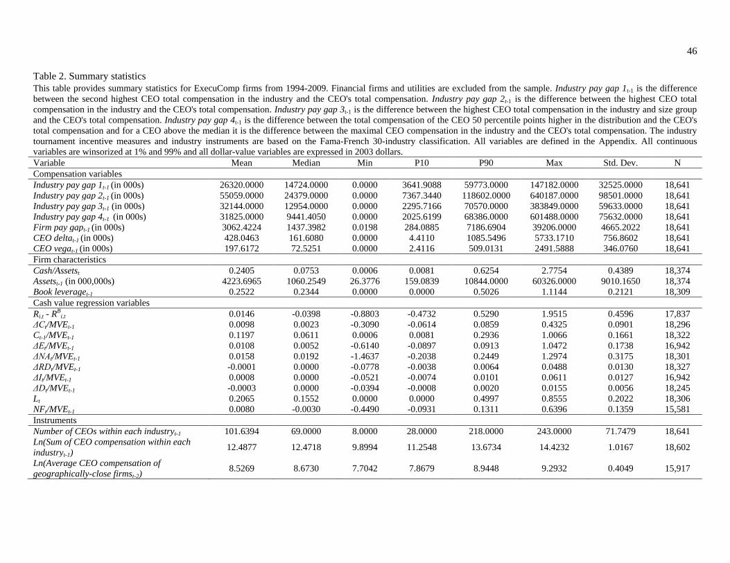
46
Table 2. Summary statistics
This table provides summary statistics for ExecuComp firms from 1994-2009. Financial firms and utilities are excluded from the sample. Industry pay gap 1t-1 is the difference
between the second highest CEO total compensation in the industry and the CEO's total compensation. Industry pay gap 2t-1 is the difference between the highest CEO total
compensation in the industry and the CEO's total compensation. Industry pay gap 3t-1 is the difference between the highest CEO total compensation in the industry and size group
and the CEO's total compensation. Industry pay gap 4t-1 is the difference between the total compensation of the CEO 50 percentile points higher in the distribution and the CEO's
total compensation and for a CEO above the median it is the difference between the maximal CEO compensation in the industry and the CEO's total compensation. The industry
tournament incentive measures and industry instruments are based on the Fama-French 30-industry classification. All variables are defined in the Appendix. All continuous
variables are winsorized at 1% and 99% and all dollar-value variables are expressed in 2003 dollars.
Variable Mean Median Min P10 P90 Max Std. Dev. N
Compensation variables
Industry pay gap 1t-1 (in 000s) 26320.0000 14724.0000 0.0000 3641.9088 59773.0000 147182.0000 32525.0000 18,641
Industry pay gap 2t-1 (in 000s) 55059.0000 24379.0000 0.0000 7367.3440 118602.0000 640187.0000 98501.0000 18,641
Industry pay gap 3t-1 (in 000s) 32144.0000 12954.0000 0.0000 2295.7166 70570.0000 383849.0000 59633.0000 18,641
Industry pay gap 4t-1 (in 000s) 31825.0000 9441.4050 0.0000 2025.6199 68386.0000 601488.0000 75632.0000 18,641
Firm pay gapt-1 (in 000s) 3062.4224 1437.3982 0.0198 284.0885 7186.6904 39206.0000 4665.2022 18,641
CEO deltat-1 (in 000s) 428.0463 161.6080 0.0000 4.4110 1085.5496 5733.1710 756.8602 18,641
CEO vegat-1 (in 000s) 197.6172 72.5251 0.0000 2.4116 509.0131 2491.5888 346.0760 18,641
Firm characteristics
Cash/Assetst 0.2405 0.0753 0.0006 0.0081 0.6254 2.7754 0.4389 18,374
Assetst-1 (in 000,000s) 4223.6965 1060.2549 26.3776 159.0839 10844.0000 60326.0000 9010.1650 18,374
Book leveraget-1 0.2522 0.2344 0.0000 0.0000 0.5026 1.1144 0.2121 18,309
Cash value regression variables
Ri,t - RB
i,t 0.0146 -0.0398 -0.8803 -0.4732 0.5290 1.9515 0.4596 17,837
ΔCt/MVEt-1 0.0098 0.0023 -0.3090 -0.0614 0.0859 0.4325 0.0901 18,296
Ct-1/MVEt-1 0.1197 0.0611 0.0006 0.0081 0.2936 1.0066 0.1661 18,322
ΔEt/MVEt-1 0.0108 0.0052 -0.6140 -0.0897 0.0913 1.0472 0.1738 16,942
ΔNAt/MVEt-1 0.0158 0.0192 -1.4637 -0.2038 0.2449 1.2974 0.3175 18,301
ΔRDt/MVEt-1 -0.0001 0.0000 -0.0778 -0.0038 0.0064 0.0488 0.0130 18,327
ΔIt/MVEt-1 0.0008 0.0000 -0.0521 -0.0074 0.0101 0.0611 0.0127 16,942
ΔDt/MVEt-1 -0.0003 0.0000 -0.0394 -0.0008 0.0020 0.0155 0.0056 18,245
Lt 0.2065 0.1552 0.0000 0.0000 0.4997 0.8555 0.2022 18,306
NFt/MVEt-1 0.0080 -0.0030 -0.4490 -0.0931 0.1311 0.6396 0.1359 15,581
Instruments
Number of CEOs within each industryt-1 101.6394 69.0000 8.0000 28.0000 218.0000 243.0000 71.7479 18,641
Ln(Sum of CEO compensation within each
industryt-1) 12.4877 12.4718 9.8994 11.2548 13.6734 14.4232 1.0167 18,602
Ln(Average CEO compensation of
geographically-close firmst-2) 8.5269 8.6730 7.7042 7.8679 8.9448 9.2932 0.4049 15,917

47
Table 3. The marginal value of cash and industry tournament incentives (ITI): Using primary ITI measure
This table presents results of OLS and instrumental variables (IV) estimation of ITI on the marginal value of cash using ExecuComp firms from 1994 – 2009. Financial firms
and utilities are excluded. The dependent variable is the annual excess stock return of the firm relative to the Fama and French (1993) 25 size and book-to-market portfolios.
Industry pay gap 1t-1 is the difference between the second highest CEO total compensation in the industry and the CEO's total compensation. Models 1 and 6 are the benchmark
Faulkender and Wang (2006) specification. Models 2, 3, 7, and 8 use dummy Industry pay gap 1t-1, where Industry pay gap 1t-1 is equal to one if its continuous value is above
the sample median and zero otherwise. Models 4, 5, 9, and 10 use the natural logarithm of continuous Industry pay gap 1t-1. All other incentive variables and control variables
are defined in the Appendix. Models 1 – 5 contain year fixed effects and two-digit SIC industry fixed effects, and Models 6 – 10 contain year fixed effects and firm fixed
effects. All continuous variables are winsorized at 1% and 99% and all dollar-value variables are expressed in 2003 dollars. p-values based on robust standard errors clustered
by firm are in parentheses. ***, **, and * denote significance at the 1%, 5%, and 10% levels, respectively.
Fixed effects Industry fixed effects Firm fixed effects
ITI measure
Dummy industry pay
gap 1t-1
Continuous industry pay
gap 1t-1
Dummy industry pay
gap 1t-1
Continuous industry pay
gap 1t-1
Estimation type FW Model OLS 2SLS
OLS 2SLS
FW Model OLS 2SLS
OLS 2SLS
(1) (2) (3) (4) (5) (6) (7) (8) (9) (10)
ΔCt/MVEt-1 1.8818*** 1.6820*** 1.3556***
0.7651 -0.3396
2.0699*** 1.9030*** 1.3973***
0.9854 0.4213
(0.0000) (0.0000) (0.0004)
(0.2917) (0.6726)
(0.0000) (0.0000) (0.0004)
(0.1409) (0.5911)
Ln(Industry pay gap 1t-1 )x
ΔCt/MVEt-1 0.1211 0.4980***
0.0900 0.1942***
0.0875 0.4506***
0.0985* 0.1503**
(0.2763) (0.0025)
(0.1556) (0.0071)
(0.4127) (0.0072)
(0.0941) (0.0387)
Ln(Industry pay gap 1t-1) -0.0222** -0.0833***
-0.0218*** -0.0387***
-0.0060 -0.4330***
-0.0117* -0.2037***
(0.0127) (0.0002)
(0.0000) (0.0003)
(0.5774) (0.0002)
(0.0517) (0.0002)
Ln(Firm gap gapt-1)x
ΔCt/MVEt-1 0.0099 0.0231
0.0250 0.0350
0.0012 0.0314
0.0041 0.0116
(0.8506) (0.6553)
(0.6528) (0.5308)
(0.9817) (0.5616)
(0.9415) (0.8344)
Ln(Firm pay gapt-1) 0.0081** 0.0048
0.0066* 0.0042
-0.0191*** -0.0345***
-0.0186*** -0.0390***
(0.0149) (0.1620)
(0.0609) (0.2519)
(0.0000) (0.0000)
(0.0002) (0.0000)
CEO deltat-1 x ΔCt/MVEt-1 0.0003*** 0.0003***
0.0003*** 0.0003**
0.0003*** 0.0002*
0.0003** 0.0003**
(0.0034) (0.0063)
(0.0073) (0.0142)
(0.0096) (0.0511)
(0.0312) (0.0488)
CEO deltat-1 -0.0000*** -0.0000**
-0.0000*** -0.0000***
-0.0000*** -0.0000***
-0.0000*** -0.0000***
(0.0064) (0.0124)
(0.0047) (0.0080)
(0.0003) (0.0018)
(0.0003) (0.0018)
CEO vegat-1 x ΔCt/MVEt-1 -0.0004 -0.0004
-0.0005 -0.0005
-0.0003 -0.0003
-0.0003 -0.0004
(0.1508) (0.2154)
(0.1365) (0.1746)
(0.2767) (0.4423)
(0.3489) (0.2593)
CEO vegat-1 -0.0000 -0.0000*
-0.0000* -0.0000**
-0.0001*** -0.0002***
-0.0002*** -0.0002***
(0.1041) (0.0614)
(0.0762) (0.0482)
(0.0000) (0.0000)
(0.0000) (0.0000)
ΔEt/MVEt-1 0.5207*** 0.5192*** 0.5119***
0.5255*** 0.5232***
0.3973*** 0.3948*** 0.3880***
0.4028*** 0.4018***
(0.0000) (0.0000) (0.0000)
(0.0000) (0.0000)
(0.0000) (0.0000) (0.0000)
(0.0000) (0.0000)
ΔNAt/MVEt-1 0.1948*** 0.1931*** 0.1920***
0.1905*** 0.1895***
0.1317*** 0.1289*** 0.1245***
0.1265*** 0.1140***
(0.0000) (0.0000) (0.0000)
(0.0000) (0.0000)
(0.0000) (0.0000) (0.0000)
(0.0000) (0.0000)
ΔRDt/MVEt-1 0.4676 0.4717 0.4734
0.5166 0.5024
-0.1571 -0.1403 -0.1844
-0.1269 -0.1764

48
(0.2714) (0.2654) (0.2635)
(0.2272) (0.2408)
(0.7183) (0.7465) (0.6868)
(0.7716) (0.6891)
ΔIt/MVEt-1 -2.2860*** -2.2408*** -2.2335***
-2.2093*** -2.2069***
-1.0729** -0.9412* -1.0134**
-0.9665* -0.8780*
(0.0000) (0.0000) (0.0000)
(0.0000) (0.0000)
(0.0319) (0.0557) (0.0406)
(0.0542) (0.0846)
ΔDt/MVEt-1 0.2598 0.3411 0.4882
0.3790 0.4116
-1.5023** -1.2076 -0.8469
-1.2726 -1.2962
(0.7191) (0.6368) (0.4942)
(0.6175) (0.5865)
(0.0494) (0.1108) (0.2710)
(0.1024) (0.1123)
Ct-1/MVEt-1 0.4869*** 0.4838*** 0.4989***
0.4904*** 0.4984***
1.2174*** 1.1479*** 1.1414***
1.1656*** 1.1661***
(0.0000) (0.0000) (0.0000)
(0.0000) (0.0000)
(0.0000) (0.0000) (0.0000)
(0.0000) (0.0000)
Lt -0.5293*** -0.5471*** -0.5613***
-0.5525*** -0.5599***
-1.1590*** -1.2063*** -1.2222***
-1.2018*** -1.2247***
(0.0000) (0.0000) (0.0000)
(0.0000) (0.0000)
(0.0000) (0.0000) (0.0000)
(0.0000) (0.0000)
NFt/MVEt-1 -0.1766*** -0.1730*** -0.1685***
-0.1749*** -0.1722***
-0.0821* -0.0671 -0.0551
-0.0661 -0.0438
(0.0000) (0.0001) (0.0001)
(0.0001) (0.0001)
(0.0703) (0.1388) (0.2453)
(0.1447) (0.3467)
Ct-1/MVEt-1 x ΔCt/MVEt-1 -0.2848 -0.2617 -0.2920
-0.2676 -0.3031
-0.5685*** -0.5287** -0.4931**
-0.5870*** -0.6259***
(0.1887) (0.2268) (0.1792)
(0.2487) (0.1905)
(0.0070) (0.0116) (0.0195)
(0.0086) (0.0048)
Lt x ΔCt/MVEt-1 -1.7639*** -1.7135*** -1.5487***
-1.6773*** -1.5735***
-1.6468*** -1.5755*** -1.3729***
-1.5507*** -1.5234***
(0.0000) (0.0000) (0.0000)
(0.0000) (0.0000)
(0.0000) (0.0000) (0.0000)
(0.0000) (0.0000)
Constant 0.0982*** 0.0520* 0.0708**
0.2479*** 0.4076***
(0.0000) (0.0653) (0.0137)
(0.0000) (0.0001)
Year Fixed Effects Yes Yes Yes
Yes Yes
Yes Yes Yes
Yes Yes
Industry Fixed Effects Yes Yes Yes
Yes Yes
No No No
No No
Firm Fixed Effects No No No
No No
Yes Yes Yes
Yes Yes
Number of Observations 13,917 13,917 13,882
13,326 13,326
13,917 13,917 13,669
13,326 13,102
R2 0.220 0.222 0.218
0.223 0.222
0.275 0.286 0.189
0.288 0.230
1st Stage: Dependent variable is Ln(Industry pay gap 1t-1)x ΔCt/MVEt-1
Number of CEOs within
each industryt-1 x
ΔCt/MVEt-1
-0.0005
-0.0034***
-0.0004
-0.0032***
(0.1693)
(0.0000)
(0.3159)
(0.0000)
Number of CEOs within
each industryt-1 0.0000*
0.0000*
0.0001***
0.0002***
(0.0972)
(0.0516)
(0.0012)
(0.0000)
Ln(Sum of CEO
compensation within each
industryt-1) x ΔCt/MVEt-1
0.3858***
1.0418***
0.3763***
1.0225***
(0.0000)
(0.0000)
(0.0000)
(0.0000)
1st Stage: Dependent variable is Ln(Industry pay gap 1t-1)
Number of CEOs within
each industryt-1 x
ΔCt/MVEt-1
-0.0018**
-0.0020
-0.0010
-0.0007
(0.0175)
(0.2094)
(0.1827)
(0.6614)
Number of CEOs within
each industryt-1 0.0042***
0.0091***
0.0033***
0.0069***

49
(0.0000)
(0.0000)
(0.0000)
(0.0000)
Ln(Sum of CEO
compensation within each
industryt-1) x ΔCt/MVEt-1
0.1788***
0.1548
0.1387**
0.1042
(0.0008)
(0.2025)
(0.0101)
(0.4032)
Anderson-Rubin Wald F-
statistic for joint relevance 7.846***
7.132***
6.396***
5.786***
Hansen's J-statistic
0.0204
0.282
0.130
0.756
Difference in Sargan-
Hansen statistics (test for
endogeneity)
17.10***
9.567***
17.25***
12.95***
First-stage F-statistics:
Ln(Industry pay gap 1t-1)x
ΔCt/MVEt-1 363.93***
394.86***
352.35***
351.00***
Ln(Industry pay gap 1t-1) 693.37***
915.94***
52.61***
89.77***
The marginal value of cash for the average firm:
Marginal value of $1
(average firm) $1.43
$1.53
Marginal value of $1 (high
industry pay gap) $1.68
$1.76
Marginal value of $1 (low
industry pay gap) $1.18 $1.31

50
Table 4. The marginal value of cash and industry tournament incentives (ITI): Using alternative ITI measures This table presents results of OLS and instrumental variables (IV) estimation of ITI on the marginal value of cash using alternative ITI
measures and ExecuComp firms from 1994 – 2009. Financial firms and utilities are excluded. The dependent variable is the annual
excess stock return of the firm relative to the Fama and French (1993) 25 size and book-to-market portfolios. Models 1 and 4 use
Industry pay gap 2t-1; Models 2 and 5 use Industry pay gap 3t-1; Models 3 and 6 use Industry pay gap 4t-1. Models 1 – 3 contain year
fixed effects and two-digit SIC industry fixed effects, and Models 4 – 6 contain year fixed effects and firm fixed effects. All variables
are defined in the Appendix. The continuous variables are winsorized at 1% and 99% and all dollar-value variables are expressed in
2003 dollars. p-values based on robust standard errors clustered by firm are in parentheses. ***, **, and * denote significance at the 1%,
5%, and 10% levels, respectively. Industry fixed effects Firm fixed effects
Industry pay
gap 2t-1
Industry pay
gap 3t-1
Industry pay
gap 4t-1
Industry pay
gap 2t-1
Industry pay
gap 3t-1
Industry pay
gap 4t-1
Estimation type (1) (2) (3) (4) (5) (6)
Ln(Industry pay gap 2t-1)x
ΔCt/MVEt-1 0.2066***
0.1287*
(0.0067)
(0.0987)
Ln(Industry pay gap 2t-1) -0.0384***
-0.1561***
(0.0003)
(0.0003)
Ln(Industry pay gap 3t-1)x
ΔCt/MVEt-1 0.2215***
0.1445*
(0.0033)
(0.0563)
Ln(Industry pay gap 3t-1)
-0.0372***
-0.1456***
(0.0002)
(0.0002)
Ln(Industry pay gap 4t-1)x
ΔCt/MVEt-1 0.3123***
0.2287*
(0.0076)
(0.0520)
Ln(Industry pay gap 4t-1) -0.0527***
-0.1930***
(0.0003)
(0.0005)
ΔCt/MVEt-1 -0.5397 -0.2327 0.2609
0.4493 0.5873 0.8531
(0.5364) (0.7515) (0.6891)
(0.6050) (0.4147) (0.1833)
Constant 0.4250*** 0.3511*** 0.2808***
(0.0001) (0.0001) (0.0001)
Controls Yes Yes Yes
Yes Yes Yes
Year Fixed Effects Yes Yes Yes
Yes Yes Yes
Industry Fixed Effects Yes Yes Yes
No No No
Firm Fixed Effects No No No
Yes Yes Yes
Number of Observations 13,626 13,349 13,626
13,405 13,121 13,405
R2 0.222 0.212 0.208
0.242 0.223 0.169
Anderson-Rubin Wald F-statistic
for joint relevance 7.365*** 8.325*** 7.365***
6.108*** 6.222*** 6.108***
Hansen's J-statistic 0.203 0.00151 0.0128
1.439 0.256 0.599
Difference in Sargan-Hansen
statistics (test for endogeneity) 9.720*** 32.00*** 21.60***
12.44*** 17.61*** 16.18***
First-stage F-statistics:
Ln(Industry pay gapt-1)x
ΔCt/MVEt-1 197.09*** 151.54*** 84.86***
173.62*** 133.13*** 73.57***
Ln(Industry pay gapt-1) 643.53*** 223.43*** 142.67*** 106.26*** 68.57*** 29.18***
Instruments used in IV (2SLS) Number of CEOs within each industryt-1
Number of CEOs within each industryt-1 x ΔCt/MVEt-1
Ln(Sum of CEO compensation within each industry t-1) x ΔCt/MVEt-1

51
Table 5. The marginal value of cash and industry tournament incentives (ITI): Using difference-in-differences (tariff cut)
specifications and primary ITI measure
This table presents results of OLS difference-in-differences estimation of ITI on the marginal value of cash following large reductions in
import tariffs using ExecuComp firms from 1994 – 2006. Tariff data are available for manufacturing firms (2000-3999 SIC range) until
2006. The dependent variable is the annual excess stock return of the firm relative to the Fama and French (1993) 25 size and book-to-
market portfolios. Ln(Industry pay gap 1)t-1 is the natural logarithm of Industry pay gap 1t-1, where Industry pay gap 1t-1 is the difference
between the second highest CEO total compensation in the industry and the CEO's total compensation. Following Fresard (2010), we define
tariff reductions (Cut dummy) using three different cut-offs. Specifically, a tariff "cut" occurs in a specific industry-year when a negative
change in the tariff rate is 2 (Models 1 and 4), 2.5 (Models 2 and 5), or 3 times (Models 3 and 6) larger than its median change. For these
three definitions, Cut dummyt = 1 if an industry had experienced a tariff cut in the year. To make sure that large tariff reductions truly
reflect non-transitory changes in the competitive environment, we exclude tariff cuts that are followed by equivalently large increases in
tariffs over the two subsequent years. All other incentive variables and control variables are defined in the Appendix. Models 1 – 3 contain
year fixed effects and two-digit SIC industry fixed effects. Models 4 – 6 contain year fixed effects and firm fixed effects. All continuous
variables are winsorized at 1% and 99% and all dollar-value variables are expressed in 2003 dollars. p-values based on robust standard
errors clustered by firm are in parentheses. ***, **, and * denote significance at the 1%, 5%, and 10% levels, respectively.
Fixed effects Industry fixed effects
Firm fixed effects
Cut dummy
CUT 2 x
Median
Change
CUT 2.5 x
Median
Change
CUT 3 x
Median
Change
CUT 2 x
Median
Change
CUT 2.5 x
Median
Change
CUT 3 x
Median
Change
(1) (2) (3) (4) (5) (6)
Ln(Industry pay gap 1t-1) x
ΔCt/MVEt-1 x Cut dummyt 0.4602** 0.5720** 0.6341***
0.3807 0.4398* 0.5026*
(0.0500) (0.0120) (0.0060)
(0.1365) (0.0849) (0.0550)
Ln(Industry pay gap 1t-1) x Cut
dummyt 0.0396** 0.0402** 0.0507***
0.0413** 0.0437** 0.0566***
(0.0114) (0.0144) (0.0025)
(0.0218) (0.0217) (0.0042)
Ln(Industry pay gap 1t-1) x
ΔCt/MVEt-1 0.0611 0.0440 0.0363
0.1041 0.0936 0.0820
(0.6355) (0.7282) (0.7736)
(0.3768) (0.4183) (0.4776)
Ln(Industry pay gap 1t-1) -0.0322*** -0.0316*** -0.0332***
-0.0298** -0.0291** -0.0312**
(0.0005) (0.0006) (0.0003)
(0.0180) (0.0205) (0.0123)
Cut dummyt x ΔCt /MVEt-1 -3.9503* -5.0196** -5.6307**
-3.0658 -3.6453 -4.3049*
(0.0852) (0.0238) (0.0124)
(0.2130) (0.1372) (0.0886)
Cut dummyt -0.3352** -0.3407** -0.4353***
-0.3322** -0.3553** -0.4769***
(0.0200) (0.0257) (0.0049)
(0.0456) (0.0442) (0.0093)
Ln(Firm gap gapt-1) x ΔCt/MVEt-1 0.1917* 0.1872* 0.1840*
0.1330 0.1291 0.1259
(0.0788) (0.0849) (0.0901)
(0.2416) (0.2545) (0.2670)
Ln(Firm pay gapt-1) 0.0110 0.0108 0.0109
-0.0249** -0.0248** -0.0242**
(0.1338) (0.1384) (0.1359)
(0.0195) (0.0197) (0.0231)
CEO deltat-1 x ΔCt/MVEt-1 0.0007** 0.0007** 0.0007**
0.0004 0.0004 0.0004
(0.0354) (0.0414) (0.0443)
(0.1624) (0.1766) (0.1796)
CEO deltat-1 -0.0000* -0.0000 -0.0000
-0.0000 -0.0000 -0.0000
(0.0987) (0.1055) (0.1109)
(0.1301) (0.1355) (0.1321)
CEO vegat-1 x ΔCt/MVEt-1 -0.0014* -0.0013* -0.0013*
-0.0007 -0.0007 -0.0006
(0.0514) (0.0577) (0.0681)
(0.3806) (0.3873) (0.4151)
CEO vegat-1 -0.0000 -0.0000 -0.0000
-0.0002*** -0.0002*** -0.0002***
(0.5818) (0.5687) (0.5393)
(0.0000) (0.0000) (0.0000)
ΔCt/MVEt-1 -0.0846 0.1355 0.2412
-0.1109 0.0551 0.2149
(0.9537) (0.9250) (0.8668)
(0.9316) (0.9656) (0.8660)
ΔEt/MVEt-1 0.5919*** 0.5912*** 0.5926***
0.4493*** 0.4503*** 0.4521***
(0.0000) (0.0000) (0.0000)
(0.0000) (0.0000) (0.0000)
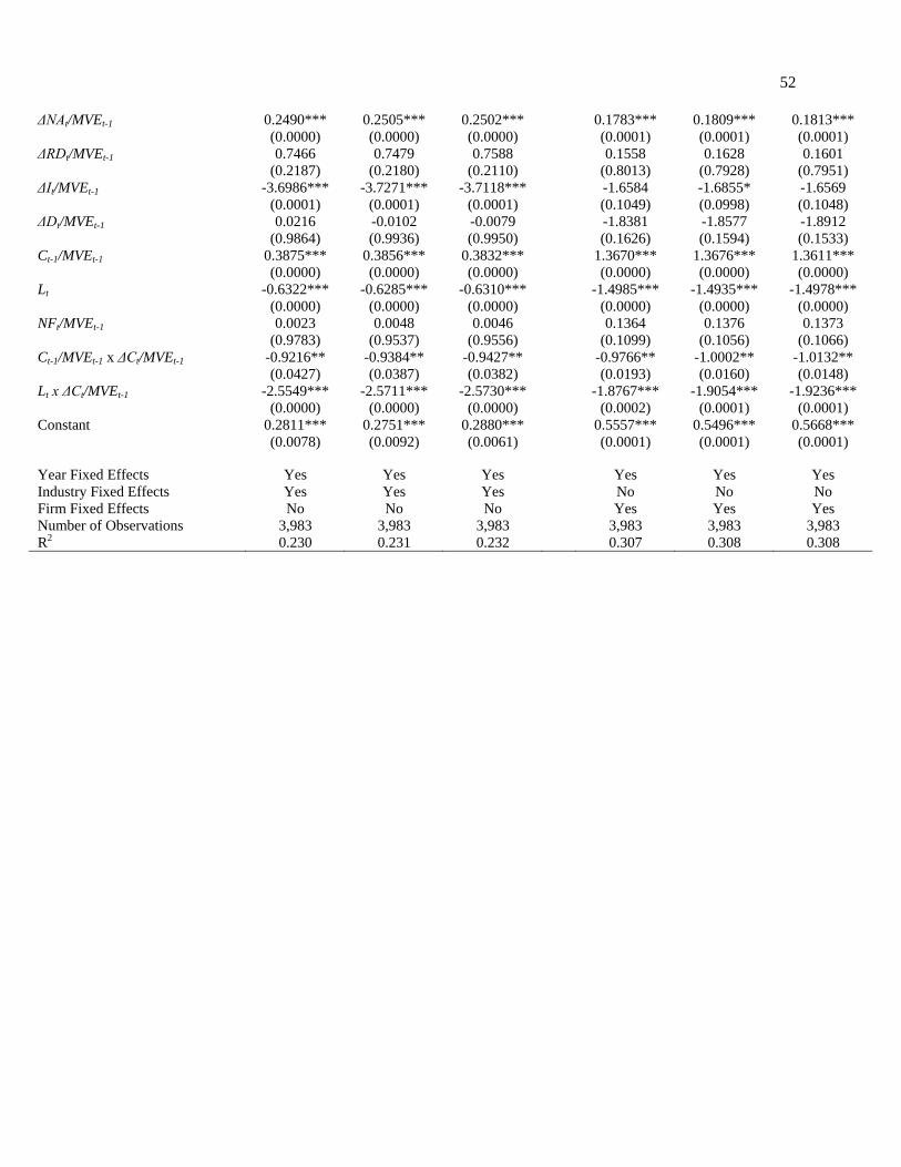
52
ΔNAt/MVEt-1 0.2490*** 0.2505*** 0.2502***
0.1783*** 0.1809*** 0.1813***
(0.0000) (0.0000) (0.0000)
(0.0001) (0.0001) (0.0001)
ΔRDt/MVEt-1 0.7466 0.7479 0.7588
0.1558 0.1628 0.1601
(0.2187) (0.2180) (0.2110)
(0.8013) (0.7928) (0.7951)
ΔIt/MVEt-1 -3.6986*** -3.7271*** -3.7118***
-1.6584 -1.6855* -1.6569
(0.0001) (0.0001) (0.0001)
(0.1049) (0.0998) (0.1048)
ΔDt/MVEt-1 0.0216 -0.0102 -0.0079
-1.8381 -1.8577 -1.8912
(0.9864) (0.9936) (0.9950)
(0.1626) (0.1594) (0.1533)
Ct-1/MVEt-1 0.3875*** 0.3856*** 0.3832***
1.3670*** 1.3676*** 1.3611***
(0.0000) (0.0000) (0.0000)
(0.0000) (0.0000) (0.0000)
Lt -0.6322*** -0.6285*** -0.6310***
-1.4985*** -1.4935*** -1.4978***
(0.0000) (0.0000) (0.0000)
(0.0000) (0.0000) (0.0000)
NFt/MVEt-1 0.0023 0.0048 0.0046
0.1364 0.1376 0.1373
(0.9783) (0.9537) (0.9556)
(0.1099) (0.1056) (0.1066)
Ct-1/MVEt-1 x ΔCt/MVEt-1 -0.9216** -0.9384** -0.9427**
-0.9766** -1.0002** -1.0132**
(0.0427) (0.0387) (0.0382)
(0.0193) (0.0160) (0.0148)
Lt x ΔCt/MVEt-1 -2.5549*** -2.5711*** -2.5730***
-1.8767*** -1.9054*** -1.9236***
(0.0000) (0.0000) (0.0000)
(0.0002) (0.0001) (0.0001)
Constant 0.2811*** 0.2751*** 0.2880***
0.5557*** 0.5496*** 0.5668***
(0.0078) (0.0092) (0.0061)
(0.0001) (0.0001) (0.0001)
Year Fixed Effects Yes Yes Yes
Yes Yes Yes
Industry Fixed Effects Yes Yes Yes
No No No
Firm Fixed Effects No No No
Yes Yes Yes
Number of Observations 3,983 3,983 3,983
3,983 3,983 3,983
R2 0.230 0.231 0.232 0.307 0.308 0.308
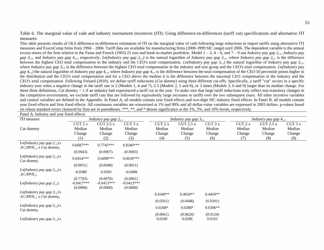
53
Table 6. The marginal value of cash and industry tournament incentives (ITI): Using difference-in-differences (tariff cut) specifications and alternative ITI
measures This table presents results of OLS difference-in-differences estimation of ITI on the marginal value of cash following large reductions in import tariffs using alternative ITI
measures and ExecuComp firms from 1994 – 2006. Tariff data are available for manufacturing firms (2000-3999 SIC range) until 2006. The dependent variable is the annual
excess return of the firm relative to the Fama and French (1993) 25 size and book-to-market portfolios. Model 1 – 3, 4 – 6, and 7 – 9 use Industry pay gap 2t-1, Industry pay
gap 3t-1, and Industry pay gap 4t-1, respectively. Ln(Industry pay gap 2t-1) is the natural logarithm of Industry pay gap 2t-1, where Industry pay gap 2t-1 is the difference
between the highest CEO total compensation in the industry and the CEO's total compensation. Ln(Industry pay gap 3t-1) the natural logarithm of Industry pay gap 3t-1,
where Industry pay gap 3t-1 is the difference between the highest CEO total compensation in the industry and size group and the CEO's total compensation. Ln(Industry pay
gap 4t-1) the natural logarithm of Industry pay gap 4t-1, where Industry pay gap 4t-1 is the difference between the total compensation of the CEO 50 percentile points higher in
the distribution and the CEO's total compensation and for a CEO above the median it is the difference between the maximal CEO compensation in the industry and the
CEO's total compensation. Following Fresard (2010), we define tariff reductions (Cut dummy) using three different cut-offs. Specifically, a tariff "cut" occurs in a specific
industry-year when a negative change in the tariff rate is 2 (Models 1, 4 and 7), 2.5 (Models 2, 5 and 8), or 3 times (Models 3, 6 and 9) larger than its median change. For
these three definitions, Cut dummyt = 1 if an industry had experienced a tariff cut in the year. To make sure that large tariff reductions truly reflect non-transitory changes in
the competitive environment, we exclude tariff cuts that are followed by equivalently large increases in tariffs over the two subsequent years. All other incentive variables
and control variables are defined in the Appendix. In Panel A, all models contain year fixed effects and two-digit SIC industry fixed effects. In Panel B, all models contain
year fixed effects and firm fixed effects. All continuous variables are winsorized at 1% and 99% and all dollar-value variables are expressed in 2003 dollars. p-values based
on robust standard errors clustered by firm are in parentheses. ***, **, and * denote significance at the 1%, 5%, and 10% levels, respectively. Panel A. Industry and year fixed effects
ITI measure Industry pay gap 2t-1 Industry pay gap 3t-1
Industry pay gap 4t-1
Cut dummy
CUT 2 x
Median
Change
CUT 2.5 x
Median
Change
CUT 3 x
Median
Change
CUT 2 x
Median
Change
CUT 2.5 x
Median
Change
CUT 3 x
Median
Change
CUT 2 x
Median
Change
CUT 2.5 x
Median
Change
CUT 3 x
Median
Change
(1) (2) (3) (4) (5) (6) (7) (8) (9)
Ln(Industry pay gap 2t-1) x
ΔCt/MVEt-1 x Cut dummyt 0.6687*** 0.7745*** 0.8340***
(0.0043) (0.0007) (0.0003)
Ln(Industry pay gap 2t-1) x
Cut dummyt 0.0454*** 0.0498*** 0.0630***
(0.0051) (0.0048) (0.0011)
Ln(Industry pay gap 2t-1) x
ΔCt/MVEt-1 -0.0380 -0.0501 -0.0498
(0.7703) (0.6970) (0.6961)
Ln(Industry pay gap 2t-1) -0.0417*** -0.0413*** -0.0423***
(0.0000) (0.0000) (0.0000)
Ln(Industry pay gap 3t-1) x
ΔCt/MVEt-1 x Cut dummyt 0.4340** 0.4034** 0.4459**
(0.0261) (0.0448) (0.0301)
Ln(Industry pay gap 3t-1) x
Cut dummyt 0.0268* 0.0288* 0.0396**
(0.0661) (0.0624) (0.0124)
Ln(Industry pay gap 3t-1) x
0.0100 0.0206 0.0161

54
ΔCt/MVEt-1
(0.9249) (0.8414) (0.8751)
Ln(Industry pay gap 3t-1)
0.0013 0.0015 0.0006
(0.8191) (0.7939) (0.9136)
Ln(Industry pay gap 4t-1) x
ΔCt/MVEt-1 x Cut dummyt 0.3859** 0.3950** 0.4027**
(0.0416) (0.0352) (0.0456)
Ln(Industry pay gap 4t-1) x
Cut dummyt 0.0269* 0.0287* 0.0387**
(0.0723) (0.0686) (0.0179)
Ln(Industry pay gap 4t-1) x
ΔCt/MVEt-1 -0.0181 -0.0179 -0.0146
(0.8820) (0.8829) (0.9042)
Ln(Industry pay gap 4t-1) -0.0073 -0.0073 -0.0082
(0.3098) (0.3077) (0.2539)
Cut dummyt x ΔCt/MVEt-1 -6.3777*** -7.4472*** -8.0308***
-3.6266* -3.3341* -3.7484*
-3.1279* -3.2121* -3.3135*
(0.0082) (0.0015) (0.0008)
(0.0556) (0.0872) (0.0608)
(0.0783) (0.0666) (0.0813)
Cut dummyt -0.4164*** -0.4619*** -0.5881***
-0.2150 -0.2323 -0.3309**
-0.2182 -0.2349 -0.3245**
(0.0083) (0.0079) (0.0018)
(0.1108) (0.1055) (0.0233)
(0.1141) (0.1092) (0.0315)
ΔCt/MVEt-1 0.9305 1.0920 1.1131
0.5584 0.4931 0.5490
1.0412 1.0409 1.0245
(0.5358) (0.4649) (0.4536)
(0.6520) (0.6821) (0.6455)
(0.3302) (0.3234) (0.3238)
Constant 0.4091*** 0.4057*** 0.4165***
-0.0310 -0.0318 -0.0260
0.0201 0.0205 0.0227
(0.0001) (0.0001) (0.0001)
(0.6916) (0.6842) (0.7397)
(0.7734) (0.7696) (0.7457)
Controls Yes Yes Yes
Yes Yes Yes
Yes Yes Yes
Year Fixed Effects Yes Yes Yes
Yes Yes Yes
Yes Yes Yes
Industry Fixed Effects Yes Yes Yes
Yes Yes Yes
Yes Yes Yes
Number of Observations 4,066 4,066 4,066
3,914 3,914 3,914
3,983 3,983 3,983
R2 0.233 0.234 0.236 0.230 0.230 0.231 0.227 0.227 0.228
Panel B. Firm and year fixed effects
ITI measure Industry pay gap 2t-1 Industry pay gap 3t-1
Industry pay gap 4t-1
Cut dummy
CUT 2 x
Median
Change
CUT 2.5 x
Median
Change
CUT 3 x
Median
Change
CUT 2 x
Median
Change
CUT 2.5 x
Median
Change
CUT 3 x
Median
Change
CUT 2 x
Median
Change
CUT 2.5 x
Median
Change
CUT 3 x
Median
Change
(1) (2) (3) (4) (5) (6) (7) (8) (9)
Ln(Industry pay gap 2t-1) x
ΔCt/MVEt-1 x Cut dummyt 0.6093*** 0.6823*** 0.7555***
(0.0073) (0.0025) (0.0012)
Ln(Industry pay gap 2t-1) x
Cut dummyt 0.0483*** 0.0539*** 0.0685***
(0.0066) (0.0055) (0.0013)
Ln(Industry pay gap 2t-1) x 0.0199 0.0107 0.0051

55
ΔCt/MVEt-1
(0.8637) (0.9262) (0.9645)
Ln(Industry pay gap 2t-1) -0.0423*** -0.0414*** -0.0425***
(0.0001) (0.0001) (0.0000)
Ln(Industry pay gap 3t-1) x
ΔCt/MVEt-1 x Cut dummyt 0.3921** 0.3730* 0.4535**
(0.0447) (0.0643) (0.0296)
Ln(Industry pay gap 3t-1) x
Cut dummyt 0.0409** 0.0437** 0.0569***
(0.0180) (0.0175) (0.0031)
Ln(Industry pay gap 3t-1) x
ΔCt/MVEt-1 0.0146 0.0195 0.0066
(0.8750) (0.8278) (0.9409)
Ln(Industry pay gap 3t-1)
-0.0163** -0.0156* -0.0164**
(0.0415) (0.0523) (0.0418)
Ln(Industry pay gap 4t-1) x
ΔCt/MVEt-1 x Cut dummyt 0.3606* 0.3682** 0.4373**
(0.0511) (0.0486) (0.0307)
Ln(Industry pay gap 4t-1) x
Cut dummyt 0.0378** 0.0404** 0.0521***
(0.0319) (0.0301) (0.0083)
Ln(Industry pay gap 4t-1) x
ΔCt/MVEt-1 -0.0653 -0.0666 -0.0767
(0.5730) (0.5617) (0.5025)
Ln(Industry pay gap 4t-1) -0.0179** -0.0178** -0.0180**
(0.0466) (0.0473) (0.0441)
Cut dummyt x ΔCt/MVEt-1 -5.6241** -6.3722*** -7.1525***
-3.1340* -2.9645 -3.7727*
-2.7988 -2.8820* -3.5917*
(0.0149) (0.0054) (0.0027)
(0.0930) (0.1222) (0.0595)
(0.1038) (0.0964) (0.0604)
Cut dummyt -0.4280** -0.4876** -0.6319***
-0.3301** -0.3568** -0.4808***
-0.3033* -0.3285* -0.4375**
(0.0132) (0.0103) (0.0025)
(0.0386) (0.0365) (0.0068)
(0.0620) (0.0575) (0.0166)
ΔCt/MVEt-1 0.6930 0.8419 0.9435
0.9051 0.8988 1.0509
1.5884 1.6099 1.7054*
(0.6031) (0.5271) (0.4748)
(0.4444) (0.4325) (0.3518)
(0.1283) (0.1145) (0.0872)
Constant 0.6995*** 0.6920*** 0.7008***
0.4251*** 0.4186*** 0.4225***
0.3635*** 0.3628*** 0.3613***
(0.0000) (0.0000) (0.0000)
(0.0002) (0.0002) (0.0002)
(0.0000) (0.0000) (0.0000)
Controls Yes Yes Yes
Yes Yes Yes
Yes Yes Yes
Year Fixed Effects Yes Yes Yes
Yes Yes Yes
Yes Yes Yes
Firm Fixed Effects Yes Yes Yes
Yes Yes Yes
Yes Yes Yes
Number of Observations 4,066 4,066 4,066
3,914 3,914 3,914
3,983 3,983 3,983
R2 0.310 0.311 0.312 0.311 0.311 0.312 0.306 0.306 0.307

56
Table 7. The marginal value of cash and industry tournament incentive (ITI): using difference-in-differences (non-competition agreement enforceability) specifications
This table presents results of OLS difference-in-difference estimation of ITI on the marginal value of cash following the change in non-competition agreement enforceability using
ExecuComp firms from 1994 – 2009. The dependent variable is the annual excess stock return of the firm relative to the Fama and French (1993) 25 size and book-to-market portfolios.
Ln(Industry pay gap 1)t-1 is the natural logarithm of Industry pay gap 1t-1, where Industry pay gap 1t-1 is the difference between the second highest CEO total compensation in the
industry and the CEO's total compensation. Ln(Industry pay gap 2t-1) is the natural logarithm of Industry pay gap 2t-1, where Industry pay gap 2t-1 is the difference between the highest
CEO total compensation in the industry and the CEO's total compensation. Ln(Industry pay gap 3t-1) the natural logarithm of Industry pay gap 3t-1, where Industry pay gap 3t-1 is the
difference between the highest CEO total compensation in the industry and size group and the CEO's total compensation. Ln(Industry pay gap 4t-1) the natural logarithm of Industry pay
gap 4t-1, where Industry pay gap 4t-1 is the difference between the total compensation of the CEO 50 percentile points higher in the distribution and the CEO's total compensation and for
a CEO above the median it is the difference between the maximal CEO compensation in the industry and the CEO's total compensation. Consistent with Garmaise (2011), Increased
enforceabilityt-1 takes the value of one for firms in Florida from 1997 on, takes the value of negative one for firms in Texas from 1995 on and for firms in Louisiana in 2002-2003, and is
set equal to zero otherwise. #in-state competitors is the number of firms within the same industry and state. We also include as additional controls State unemployment rate and State
personal per capita income in the year provided by the Bureau of Economic Analysis. All other incentive variables and control variables are defined in the Appendix. All continuous
variables are winsorized at 1% and 99% and all dollar-value variables are expressed in 2003 dollars. p-values based on robust standard errors clustered by firm are in parentheses. ***,
**, and * denote significance at the 1%, 5%, and 10% levels, respectively. #in-state competitors > 10 #in-state competitors > 30 #in-state competitors > 100
Industry
pay gap1
Industry
pay gap2
Industry
pay gap3
Industry
pay gap4
Industry
pay gap1
Industry
pay gap2
Industry
pay gap3
Industry
pay gap4
Industry
pay gap1
Industry
pay gap2
Industry
pay gap3
Industry
pay gap4
(1) (2) (3) (4) (5) (6) (7) (8) (9) (10) (11) (12)
Ln(Industry pay gap 1t-1) x
ΔCt/MVEt-1 x Increased
enforceabilityt-1
-0.4549*
-0.5861*
-1.1823*
(0.0587)
(0.0548)
(0.0568)
Ln(Industry pay gap 1t-1) x
Increased enforceabilityt-1 0.0315**
0.0138
0.1507***
(0.0248)
(0.6231)
(0.0020)
Ln(Industry pay gap 1t-1) x
ΔCt/MVEt-1 0.0146
-0.0411
0.0056
(0.9071)
(0.8015)
(0.9878)
Ln(Industry pay gap 1t-1) -0.0019
0.0042
0.0194
(0.8194)
(0.7319)
(0.4333)
Ln(Industry pay gap 2t-1) x
ΔCt/MVEt-1 x Increased
enforceabilityt-1
-0.2148
-0.6085*
-1.0436*
(0.3068)
(0.0896)
(0.0568)
Ln(Industry pay gap 2t-1) x
Increased enforceabilityt-1 0.0255*
0.0004
0.1348***
(0.0811)
(0.9878)
(0.0028)
Ln(Industry pay gap 2t-1) x
ΔCt/MVEt-1 0.0521
-0.0483
0.0724
(0.6028)
(0.7351)
(0.8081)
Ln(Industry pay gap 2t-1)
-0.0024
0.0011
0.0265
(0.7332)
(0.9197)
(0.2424)

57
Ln(Industry pay gap 3t-1) x
ΔCt/MVEt-1 x Increased
enforceabilityt-1
-0.4577***
-0.7634***
-1.1312**
(0.0080)
(0.0082)
(0.0295)
Ln(Industry pay gap 3t-1) x
Increased enforceabilityt-1 0.0285**
0.0359
0.2231***
(0.0125)
(0.1065)
(0.0000)
Ln(Industry pay gap 3t-1) x
ΔCt/MVEt-1 -0.0125
-0.0736
0.0170
(0.8885)
(0.5804)
(0.9493)
Ln(Industry pay gap 3t-1)
0.0114*
0.0307***
0.0366*
(0.0536)
(0.0023)
(0.0744)
Ln(Industry pay gap 4t-1) x
ΔCt/MVEt-1 x Increased
enforceabilityt-1
-0.0483
0.1638
0.3160
(0.7572)
(0.4243)
(0.4640)
Ln(Industry pay gap 4t-1) x
Increased enforceabilityt-1 0.0222**
0.0170
0.1210***
(0.0278)
(0.2579)
(0.0004)
Ln(Industry pay gap 4t-1) x
ΔCt/MVEt-1 0.0170
-0.0361
0.3245*
(0.8412)
(0.7471)
(0.0982)
Ln(Industry pay gap 4t-1) 0.0129**
0.0256**
0.0501**
(0.0497)
(0.0118)
(0.0126)
Increased enforceabilityt-1
x ΔCt /MVEt-1 4.4725* 2.1550 4.3971** 0.2557
5.7783* 6.3986 7.4487** -1.9152
12.6467* 11.4984* 11.1724** -2.6459
(0.0791) (0.3436) (0.0122) (0.8740)
(0.0780) (0.1042) (0.0127) (0.3751)
(0.0549) (0.0537) (0.0367) (0.5283)
Increased enforceabilityt-1 -0.3501** -0.3043* -0.3161*** -0.2435**
-0.1543 -0.0137 -0.3778 -0.1819
-1.4454*** -1.3351*** -2.0316*** -1.0324***
(0.0138) (0.0526) (0.0069) (0.0144)
(0.6034) (0.9617) (0.1086) (0.2340)
(0.0027) (0.0039) (0.0001) (0.0011)
Ct-1/MVEt-1 0.4316*** 0.4343*** 0.4330*** 0.4287***
0.5945*** 0.5887*** 0.5875*** 0.5913***
0.6141*** 0.6047*** 0.6344*** 0.6178***
(0.0000) (0.0000) (0.0000) (0.0000)
(0.0000) (0.0000) (0.0000) (0.0000)
(0.0005) (0.0006) (0.0004) (0.0009)
State unemployment ratet-1 -0.0054 -0.0064 -0.0059 -0.0052
-0.0028 -0.0031 -0.0009 -0.0003
0.0068 0.0080 0.0054 0.0097
(0.1645) (0.1051) (0.1316) (0.1833)
(0.6716) (0.6415) (0.8907) (0.9596)
(0.6778) (0.6279) (0.7348) (0.5362)
State personal income per
capitat-1 -0.0558 -0.0514 -0.0546 -0.0593
-0.1882** -0.1719* -0.1425 -0.1588*
-0.1857 -0.1390 -0.1076 -0.1755
(0.2501) (0.2926) (0.2694) (0.2264)
(0.0365) (0.0559) (0.1129) (0.0759)
(0.4048) (0.5281) (0.6366) (0.4289)
Constant 0.5498 0.5204 0.4271 0.4993
1.8267* 1.7042* 1.1337 1.4225
1.2660 0.7229 0.4834 1.1153
(0.2818) (0.3114) (0.4170) (0.3329)
(0.0676) (0.0895) (0.2589) (0.1549)
(0.5902) (0.7586) (0.8456) (0.6344)
Controls Yes Yes Yes Yes
Yes Yes Yes Yes
Yes Yes Yes Yes
Industry Fixed Effects Yes Yes Yes Yes
Yes Yes Yes Yes
Yes Yes Yes Yes
Year Fixed Effects Yes Yes Yes Yes
Yes Yes Yes Yes
Yes Yes Yes Yes
Number of Observations 5,075 5,149 5,079 5,149
2,390 2,412 2,377 2,412
760 765 754 765
R2 0.203 0.202 0.205 0.202 0.209 0.209 0.216 0.210 0.259 0.258 0.271 0.263

58
Table 8. Cash holdings and industry tournament incentives (ITI)
This table presents results on the relation between cash holdings and industry tournament incentives (ITI). The dependent variable is Cash/Assetst. Model 1-2, 3-4, 5-6, and 7-8 use
Industry pay gap 1, Industry pay gap 2, Industry pay gap 3, and Industry pay gap 4, respectively. Ln(Industry pay gap 1) is the natural logarithm of Industry pay gap 1, where Industry
pay gap 1 is the difference between the second highest CEO total compensation in the industry and the CEO's total compensation. Ln(Industry pay gap 2) is the natural logarithm of
Industry pay gap 2, where Industry pay gap 2 is the difference between the highest CEO total compensation in the industry and the CEO's total compensation. Ln(Industry pay gap 3)
the natural logarithm of Industry pay gap 3, where Industry pay gap 3 is the difference between the highest CEO total compensation in the industry and size group and the CEO's total
compensation. Ln(Industry pay gap 4) the natural logarithm of Industry pay gap 4, where Industry pay gap 4 is the difference between the total compensation of the CEO 50 percentile
points higher in the distribution and the CEO's total compensation and for a CEO above the median it is the difference between the maximal CEO compensation in the industry and the
CEO's total compensation. All other incentive variables are defined in the Appendix, and the other control variables are consistent with those used in Bates, Kahle, and Stulz (2009). All
continuous variables are winsorized at 1% and 99% and all dollar-value variables are expressed in 2003 dollars. p-values based on robust standard errors clustered by firm are in
parentheses. ***, **, and * denote significance at the 1%, 5%, and 10% levels, respectively.
Panel A. Industry and year fixed effects
ITI measure Industry pay gap1 t-1 Industry pay gap2 t-1 Industry pay gap3 t-1 Industry pay gap4 t-1
(1) (2) (3) (4) (5) (6) (7) (8)
Ln(Industry pay gap 1t-1) 0.0128** 0.0581***
(0.0429) (0.0040)
Ln(Industry pay gap 2t-1)
0.0135*** 0.0582***
(0.0054) (0.0036)
Ln(Industry pay gap 3t-1)
0.0140*** 0.0521***
(0.0003) (0.0036)
Ln(Industry pay gap 4t-1)
0.0143*** 0.0794***
(0.0001) (0.0038)
Ln(Firm pay gapt-1) 0.0198*** 0.0260***
0.0191*** 0.0232***
0.0200*** 0.0241***
0.0104** -0.0240
(0.0000) (0.0000)
(0.0000) (0.0000)
(0.0000) (0.0000)
(0.0112) (0.1285)
CEO vegat-1 0.0000 0.0000
0.0000 0.0000
0.0000 0.0000
0.0000 0.0000
(0.4809) (0.5368)
(0.5292) (0.5546)
(0.7339) (0.9469)
(0.5389) (0.6549)
CEO deltat-1 0.0000 0.0000
0.0000 0.0000
0.0000 0.0000
0.0000 0.0000
(0.5113) (0.8290)
(0.5715) (0.8994)
(0.2640) (0.4079)
(0.4419) (0.2426)
Industry sigmat 0.0272 0.0202
0.0310 0.0366
0.0277 0.0281
0.0312 0.0407*
(0.1988) (0.4064)
(0.1317) (0.1302)
(0.1822) (0.2421)
(0.1287) (0.0931)
Market-to-bookt 0.0660*** 0.0651***
0.0656*** 0.0644***
0.0658*** 0.0640***
0.0654*** 0.0624***
(0.0000) (0.0000)
(0.0000) (0.0000)
(0.0000) (0.0000)
(0.0000) (0.0000)
Ln(Assetst) -0.0869*** -0.0855***
-0.0859*** -0.0850***
-0.0911*** -0.1018***
-0.0881*** -0.0969***
(0.0000) (0.0000)
(0.0000) (0.0000)
(0.0000) (0.0000)
(0.0000) (0.0000)
Cash flow/Assetst 0.1284 0.0884
0.1238 0.0898
0.1228 0.0849
0.1181 0.0588
(0.1246) (0.3406)
(0.1368) (0.3325)
(0.1452) (0.3646)
(0.1547) (0.5110)
NWC/Assetst -0.3654*** -0.3868***
-0.3653*** -0.3833***
-0.3586*** -0.3696***
-0.3633*** -0.3728***
(0.0000) (0.0000)
(0.0000) (0.0000)
(0.0000) (0.0000)
(0.0000) (0.0000)
CAPX/Assetst -0.3547*** -0.4222***
-0.3516*** -0.4301***
-0.3227*** -0.3834***
-0.3517*** -0.4501***

59
(0.0004) (0.0004)
(0.0003) (0.0003)
(0.0008) (0.0010)
(0.0003) (0.0002)
Book leveraget -0.0146 -0.0272
-0.0154 -0.0274
-0.0104 -0.0227
-0.0161 -0.0251
(0.7269) (0.5508)
(0.7089) (0.5433)
(0.8033) (0.6192)
(0.6979) (0.5744)
R&D/Salest 1.1374*** 1.1098***
1.1377*** 1.1211***
1.1389*** 1.1327***
1.1337*** 1.0870***
(0.0000) (0.0000)
(0.0000) (0.0000)
(0.0000) (0.0000)
(0.0000) (0.0000)
Dividend dummyt 0.0036 0.0119
0.0034 0.0118
0.0040 0.0100
0.0031 0.0128
(0.7020) (0.2707)
(0.7189) (0.2731)
(0.6719) (0.3447)
(0.7367) (0.2519)
Acquisition/Assetst -0.3654*** -0.3530***
-0.3622*** -0.3550***
-0.3639*** -0.3354***
-0.3627*** -0.3707***
(0.0000) (0.0000)
(0.0000) (0.0000)
(0.0000) (0.0000)
(0.0000) (0.0000)
Constant 0.4095*** 0.0042
0.3926*** -0.0222
0.4283*** 0.1821
0.4706*** 0.2545**
(0.0000) (0.9825)
(0.0000) (0.9101)
(0.0000) (0.1630)
(0.0000) (0.0208)
Year Fixed Effects Yes Yes
Yes Yes
Yes Yes
Yes Yes
Industry Fixed Effects Yes Yes
Yes Yes
Yes Yes
Yes Yes
Number of Observations 14,877 11,874
15,188 12,130
14,881 11,898
15,188 12,130
R2 0.590 0.593
0.590 0.590
0.591 0.589
0.590 0.576
Anderson-Rubin Wald F-statistic for joint relevance
4.497***
4.532***
4.612***
4.532***
Hansen J-statistic
1.091
0.713
1.132
0.901
Difference in Sargan-Hansen statistics (test for
endogeneity) 8.074***
6.991***
6.115***
5.942***
First-stage F-statistics:
Ln(Industry pay gapt-1)
1279***
1023***
464.2***
191.4***
Instruments used in IV (2SLS) Number of CEOs within each industryt-1
Ln(Average CEO compensation of geographically-close firmst-2)
Panel B. Firm and year fixed effects
ITI measure Industry pay gap1 t-1 Industry pay gap2 t-1 Industry pay gap3 t-1 Industry pay gap4 t-1
(1) (2) (3) (4) (5) (6) (7) (8)
Ln(Industry pay gap 1t-1) 0.0077** 0.1042***
(0.0269) (0.0041)
Ln(Industry pay gap 2t-1)
0.0072*** 0.0912***
(0.0094) (0.0063)
Ln(Industry pay gap 3t-1)
0.0086*** 0.0798***
(0.0005) (0.0027)
Ln(Industry pay gap 4t-1)
0.0077*** 0.1039***
(0.0009) (0.0068)
Ln(Firm pay gapt-1) 0.0126*** 0.0227***
0.0120*** 0.0167***
0.0127*** 0.0199***
0.0080*** -0.0359**
(0.0001) (0.0000)
(0.0001) (0.0000)
(0.0000) (0.0000)
(0.0057) (0.0402)

60
CEO vegat-1 0.0000 0.0000
0.0000 0.0000
0.0000 0.0000
0.0000 0.0000
(0.5108) (0.4211)
(0.5394) (0.3220)
(0.5084) (0.5862)
(0.5529) (0.4999)
CEO deltat-1 0.0000 0.0000
0.0000 0.0000
0.0000 0.0000
0.0000 0.0000*
(0.1128) (0.2572)
(0.1821) (0.3513)
(0.1382) (0.2035)
(0.1551) (0.0763)
Industry sigmat 0.0140 0.0184
0.0154 0.0417**
0.0154 0.0337*
0.0153 0.0396**
(0.3758) (0.2733)
(0.3189) (0.0284)
(0.3284) (0.0568)
(0.3225) (0.0370)
Market-to-bookt 0.0509*** 0.0475***
0.0506*** 0.0477***
0.0502*** 0.0467***
0.0505*** 0.0471***
(0.0000) (0.0000)
(0.0000) (0.0000)
(0.0000) (0.0000)
(0.0000) (0.0000)
Ln(Assetst) -0.1523*** -0.1608***
-0.1510*** -0.1598***
-0.1538*** -0.1806***
-0.1519*** -0.1722***
(0.0000) (0.0000)
(0.0000) (0.0000)
(0.0000) (0.0000)
(0.0000) (0.0000)
Cash flow/Assetst 0.0729 0.0822
0.0697 0.0794
0.0623 0.0621
0.0680 0.0551
(0.2530) (0.2730)
(0.2735) (0.2918)
(0.3320) (0.4106)
(0.2847) (0.4633)
NWC/Assetst -0.3473*** -0.4072***
-0.3471*** -0.3875***
-0.3413*** -0.3784***
-0.3468*** -0.3960***
(0.0000) (0.0000)
(0.0000) (0.0000)
(0.0000) (0.0000)
(0.0000) (0.0000)
CAPX/Assetst 0.0495 0.0160
0.0473 -0.0226
0.0669 0.0011
0.0451 -0.0798
(0.5250) (0.8622)
(0.5380) (0.8136)
(0.3906) (0.9911)
(0.5567) (0.4685)
Book leveraget 0.1727*** 0.1699***
0.1714*** 0.1688***
0.1729*** 0.1661***
0.1719*** 0.1796***
(0.0001) (0.0004)
(0.0001) (0.0003)
(0.0001) (0.0005)
(0.0001) (0.0001)
R&D/Salest 0.4568*** 0.5046***
0.4497*** 0.4817***
0.4643*** 0.5454***
0.4507*** 0.4789***
(0.0007) (0.0008)
(0.0006) (0.0018)
(0.0006) (0.0003)
(0.0006) (0.0013)
Dividend dummyt 0.0488*** 0.0524***
0.0478*** 0.0492***
0.0469*** 0.0450***
0.0473*** 0.0426***
(0.0000) (0.0000)
(0.0000) (0.0000)
(0.0000) (0.0001)
(0.0000) (0.0009)
Acquisition/Assetst -0.1909*** -0.1839***
-0.1910*** -0.1905***
-0.2008*** -0.1710***
-0.1923*** -0.2070***
(0.0000) (0.0000)
(0.0000) (0.0000)
(0.0000) (0.0000)
(0.0000) (0.0000)
Constant 0.8937***
0.8940***
0.9025***
0.9293***
(0.0000)
(0.0000)
(0.0000)
(0.0000)
Year Fixed Effects Yes Yes
Yes Yes
Yes Yes
Yes Yes
Firm Fixed Effects Yes Yes
Yes Yes
Yes Yes
Yes Yes
Number of Observations 14,877 11,622
15,188 11,883
14,881 11,649
15,188 11,883
R2 0.300 0.250
0.299 0.236
0.300 0.233
0.299 0.164
Anderson-Rubin Wald F-statistic for joint relevance
4.217***
3.838***
4.677***
3.838***
Hansen J-statistic
0.356
0.0553
0.144
0.0360
Difference in Sargan-Hansen statistics (test for
endogeneity) 7.316***
6.950***
7.965***
6.892***
First-stage F-statistics:
Ln(Industry pay gapt-1)
110.5***
129.5***
134.0***
41.49***
Instruments used in IV (2SLS) Number of CEOs within each industryt-1
Ln(Average CEO compensation of geographically-close firmst-2)

61
Table 9. Dissipation/Accumulation of excess cash and industry tournament incentives (ITI)
This table presents results on the dissipation/accumulation of excess cash motivated by Dittmar and Mahrt-Smith (2007). The sample includes all firms that have positive excess
cash at date t. In Panel A, the dependent variable is the past change in excess cash relative to assets (ratio at t minus ratio at t-1), and in Panel B, the dependent variable is the future
change in excess cash relative to assets (ratio at t+1 minus ratio at t). Model 1-2, 3-4, 5-6, and 7-8 of both panels use Industry pay gap 1t-1, Industry pay gap 2t-1, Industry pay gap
3t-1, and Industry pay gap 4t-1, respectively. Ln(Industry pay gap 1t-1) is the natural logarithm of Industry pay gap 1t-1, where Industry pay gap 1t-1 is the difference between the
second highest CEO total compensation in the industry and the CEO's total compensation. Ln(Industry pay gap 2t-1) is the natural logarithm of Industry pay gap 2t-1, where Industry
pay gap 2t-1 is the difference between the highest CEO total compensation in the industry and the CEO's total compensation. Ln(Industry pay gap 3t-1) the natural logarithm of
Industry pay gap 3t-1, where Industry pay gap 3t-1 is the difference between the highest CEO total compensation in the industry and size group and the CEO's total compensation.
Ln(Industry pay gap 4t-1) the natural logarithm of Industry pay gap 4t-1, where Industry pay gap 4t-1 is the difference between the total compensation of the CEO 50 percentile
points higher in the distribution and the CEO's total compensation and for a CEO above the median it is the difference between the maximal CEO compensation in the industry and
the CEO's total compensation. Industry average change in excess casht is the past industry average change in excess cash divided by assets (ratio at t minus ratio at t-1). All other
incentive variables are defined in the Appendix. Excess cash is the residual from Panel A Model 9 by regressing Cash/Assetst on the median industry standard deviation of the past
10 year cash flow over assets (Industry sigmat), market-to-book ratio (Market-to-bookt), natural logarithm of firm real assets (Ln(Assets)t), cash flow to assets (Cash flow/Assetst),
net working capital to assets (NWC/Assetst), R&D to sales (R&D/Salest), capital expenditures to assets (CAPX/Assetst), long-term debt plus short-term debt divided by assets (Book
leveraget), a dummy variable if the firm pays dividends (Dividend dummyt), year dummies, and two-digit SIC industry dummies. All continuous variables are winsorized at 1% and
99% and all dollar-value variables are expressed in 2003 dollars. p-values based on robust standard errors clustered by firm are in parentheses. ***, **, and * denote significance at
the 1%, 5%, and 10% levels, respectively.
Panel A. Accumulation of excess cash
ITI measure Industry pay gap1t-1 Industry pay gap2t-1 Industry pay gap3t-1 Industry pay gap4t-1 Excess cash estimation
Estimation type OLS 2SLS
OLS 2SLS
OLS 2SLS
OLS 2SLS
(1) (2) (3) (4) (5) (6) (7) (8) (9)
Ln(Industry pay gap 1t-1) 0.0174*** 0.0308***
Industry
sigmat 0.0219
(0.0000) (0.0000)
(0.2319)
Ln(Industry pay gap 2t-1) 0.0142*** 0.0319***
Market-to-
bookt 0.0632***
(0.0000) (0.0000)
(0.0000)
Ln(Industry pay gap 3t-1) 0.0025 0.0348***
Ln(Assetst) -0.0721***
(0.2382) (0.0000)
(0.0000)
Ln(Industry pay gap 4t-1) 0.0058** 0.0425***
Cash
flow/Assetst 0.1227
(0.0410) (0.0000)
(0.1274)
Ln(Firm pay gapt-1) -
0.0110*** -0.0098***
-0.0116*** -0.0103***
-0.0139*** -0.0161***
-0.0160*** -0.0365*** NWC/Assetst -0.3515***
(0.0016) (0.0047)
(0.0005) (0.0018)
(0.0000) (0.0000)
(0.0000) (0.0000)
(0.0000)
CEO deltat-1 0.0000 0.0000
0.0000 0.0000
0.0000 -0.0000
0.0000 -0.0000 R&D/Salest 1.1936***
(0.7472) (0.8982)
(0.5932) (0.8197)
(0.5321) (0.8202)
(0.5202) (0.8379)
(0.0000)
CEO vegat-1 0.0000** 0.0000**
0.0000* 0.0000*
0.0000* 0.0000
0.0000* 0.0000** CAPX/Assetst -0.2066**
(0.0362) (0.0408)
(0.0921) (0.0916)
(0.0843) (0.2508)
(0.0798) (0.0302)
(0.0253)
Industry average change in 1.2016*** 1.1893***
1.1807*** 1.1509***
1.1948*** 1.1123***
1.2032*** 1.1508*** Book -0.0187

62
excess casht leveraget
(0.0000) (0.0000)
(0.0000) (0.0000)
(0.0000) (0.0000)
(0.0000) (0.0000)
(0.6361)
Dividend
dummyt -0.0045
(0.6341)
Constant -0.0553 -0.1916***
-0.0279 -0.2167***
0.1085*** -0.1845***
0.0928*** -0.1006** Constant 0.5409***
(0.1675) (0.0006)
(0.4945) (0.0002)
(0.0008) (0.0016)
(0.0037) (0.0220)
(0.0000)
Number of Observations 4,896 4,794
5,060 4,949
4,965 4,855
5,060 4,949
16,469
R2 0.054 0.050 0.053 0.044 0.047 0.014 0.048 0.010 0.582
Anderson-Rubin Wald F-
statistic for joint relevance 18.50***
18.76***
18.84***
18.76***
Hansen's J-statistic
0.00324
0.0240
0.935
0.632
Difference in Sargan-Hansen
statistics (test for
endogeneity)
17.65***
23.99***
34.94***
35.58***
First-stage F-statistics:
Ln(Industry pay gapt-1)
1084***
921.3***
302.7***
263.4***
Instruments used in IV
(2SLS) Number of CEOs within each industryt
Ln(Average CEO compensation of geographically-close firmst-1)
Panel B. Dissipation of excess cash
ITI measure Industry pay gap1t Industry pay gap2t
Industry pay gap3t Industry pay gap4t
Estimation type OLS 2SLS
OLS 2SLS
OLS 2SLS
OLS 2SLS
(1) (2) (3) (4) (5) (6) (7) (8)
Ln(Industry pay gap 1t) -0.0144*** -0.0381***
(0.0000) (0.0000)
Ln(Industry pay gap 2t)
-0.0120*** -0.0403***
(0.0000) (0.0000)
Ln(Industry pay gap 3t)
-0.0001 -0.0476***
(0.9562) (0.0000)
Ln(Industry pay gap 4t)
-0.0061** -0.0545***
(0.0242) (0.0000)
Ln(Firm pay gapt) 0.0048 0.0017
0.0058* 0.0031
0.0068** 0.0097***
0.0101*** 0.0358***
(0.1309) (0.6001)
(0.0577) (0.3168)
(0.0276) (0.0050)
(0.0024) (0.0000)
CEO deltat 0.0045 0.0055
0.0060 0.0084**
0.0047 0.0105***
0.0057 0.0117***
(0.2163) (0.1350)
(0.1039) (0.0279)
(0.2191) (0.0098)
(0.1314) (0.0036)
CEO vegat -0.0003 0.0016
-0.0029 -0.0041
-0.0025 0.0070
-0.0029 -0.0101
(0.9766) (0.8853)
(0.7691) (0.7003)
(0.8084) (0.5308)
(0.7648) (0.3668)
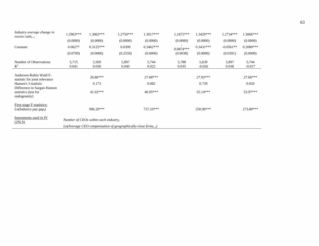
63
Industry average change in
excess casht+1 1.2963*** 1.3062***
1.2750*** 1.3017***
1.2475*** 1.3429***
1.2734*** 1.3066***
(0.0000) (0.0000)
(0.0000) (0.0000)
(0.0000) (0.0000)
(0.0000) (0.0000)
Constant 0.0627* 0.3125***
0.0399 0.3462***
-
0.0874*** 0.3431***
-0.0561** 0.2080***
(0.0709) (0.0000)
(0.2559) (0.0000)
(0.0038) (0.0000)
(0.0391) (0.0000)
Number of Observations 5,715 5,569
5,897 5,744
5,788 5,639
5,897 5,744
R2 0.041 0.030
0.040 0.022
0.035 -0.026
0.038 -0.017
Anderson-Rubin Wald F-
statistic for joint relevance 26.86***
27.68***
27.93***
27.68***
Hansen's J-statistic
0.173
0.082
0.739
0.020
Difference in Sargan-Hansen
statistics (test for
endogeneity)
41.02***
40.95***
55.14***
53.97***
First-stage F-statistics:
Ln(Industry pay gapt)
996.20***
737.10***
250.90***
273.80***
Instruments used in IV
(2SLS) Number of CEOs within each industryt
Ln(Average CEO compensation of geographically-close firmst-1)

64
Table 10. Impact of industry tournament incentives (ITI) on the uses of excess cash for investment and distribution purposes
This table presents results to examine how firms disgorge excess cash. The sample includes all firms that have positive excess cash at date t. The dependent variables are
R&D expenditures (R&D/Assetst), capital expenditures (CAPX/Assetst), acquisitions (Acquisitions/Assetst), focused acquisition expenditures (Focused
acquisitions/Assetst), and payout ((Div+Rep)/Net incomet). Focused acquisitions involve acquirer and target firms that operate in the same industry based on Fama-
French 30-industry classification. Ln(Industry pay gap1t-1) is the natural logarithm of Industry pay gap1t-1, where Industry pay gap1t-1 is the difference between the
second highest CEO total compensation in the industry and the CEO's total compensation. All other incentive variables are defined in Appendix. The control variables
include natural logarithm of firm real assets (Ln(Assetst-1)), cash flow to assets (Cash flow/Assetst-1), the median industry standard deviation of the past 10-year cash flow
over assets (Industry sigmat-1), sales growth (Sales growtht-1), and long-term debt plus short-term debt divided by assets (Book leveraget-1). Excess cash is the residual
from Table 8 Model 9 by regressing Cash/Assetst on the median industry standard deviation of the past 10 year cash flow over assets (Industry sigmat), market-to-book
ratio (Market-to-bookt), natural logarithm of firm real assets (Ln(Assetst)), cash flow to assets (Cash flow/Assetst), net working capital to assets (NWC/Assetst), R&D to
assets (R&D/Assetst), capital expenditures to assets (CAPX/Assetst), long-term debt plus short-term debt divided by assets (Book leveraget), a dummy variable if the firm
pays dividends (Dividend dummyt), year dummies, and two-digit SIC industry dummies. All continuous variables are winsorized at 1% and 99% and all dollar-value
variables are expressed in 2003 dollars. p-values based on robust standard errors clustered by firm are in parentheses. ***, **, and * denote significance at the 1%, 5%,
and 10% levels, respectively.
Investment Decisions Payout Decisions
R&D/Assetst CAPX/Assetst Acquisitions/Assetst Focused Acquisitions/Assetst (Div+Rep)/Net incomet
Estimation type OLS 2SLS OLS 2SLS OLS 2SLS OLS 2SLS
OLS 2SLS
(1) (2) (3) (4) (5) (6) (7) (8) (9) (10)
Outcome variablet-1 0.8626*** 0.8600*** 0.6431*** 0.6416*** 0.0478*** 0.0470*** 0.0353** 0.0349*
0.1055*** 0.1050***
(0.0000) (0.0000) (0.0000) (0.0000) (0.0012) (0.0014) (0.0491) (0.0516)
(0.0000) (0.0000)
Ln(Industry pay gap1t-1) 0.0013** 0.0057*** -0.0002 0.0012 0.0050** 0.0108*** 0.0053*** 0.0106***
-0.0454** -0.0711**
(0.0304) (0.0000) (0.7181) (0.2191) (0.0293) (0.0035) (0.0068) (0.0013)
(0.0297) (0.0351)
Ln(Firm pay gapt-1) -0.0001 0.0004 0.0005 0.0006 0.0084*** 0.0090*** 0.0066*** 0.0071***
0.0212 0.0185
(0.8850) (0.5173) (0.3353) (0.2050) (0.0000) (0.0000) (0.0000) (0.0000)
(0.1277) (0.1947)
CEO deltat-1 -0.0000 -0.0000 0.0000 0.0000 0.0000* 0.0000* -0.0000 -0.0000
0.0000 0.0000
(0.4091) (0.3345) (0.6371) (0.6648) (0.0739) (0.0784) (0.1577) (0.1382)
(0.3184) (0.3070)
CEO vegat-1 0.0000*** 0.0000*** 0.0000 0.0000 0.0000 0.0000 0.0000** 0.0000**
0.0001 0.0001
(0.0011) (0.0008) (0.3365) (0.3150) (0.9303) (0.9134) (0.0416) (0.0377)
(0.4344) (0.4372)
Ln(Assetst-1) -0.0021*** -0.0018*** -0.0023*** -0.0022*** -0.0098*** -0.0094*** -0.0060*** -0.0056***
-0.0003 -0.0022
(0.0002) (0.0008) (0.0000) (0.0000) (0.0000) (0.0000) (0.0000) (0.0000)
(0.9835) (0.8585)
Cash flow/Assetst-1 -0.0129 -0.0137 0.0150*** 0.0150*** 0.0329* 0.0330* 0.0328* 0.0331*
0.6879*** 0.6883***
(0.1944) (0.1690) (0.0084) (0.0078) (0.0985) (0.0955) (0.0745) (0.0689)
(0.0000) (0.0000)
Industry sigmat-1 0.0077** 0.0074** 0.0028 0.0027 0.0162* 0.0158* 0.0267*** 0.0260***
-0.0388 -0.0380
(0.0130) (0.0161) (0.2137) (0.2317) (0.0545) (0.0594) (0.0027) (0.0030)
(0.6474) (0.6538)
Sales growtht-1 -0.0097** -0.0094** 0.0076*** 0.0077*** 0.0503*** 0.0506*** 0.0144 0.0148
-0.3542*** -0.3561***

65
(0.0217) (0.0243) (0.0058) (0.0049) (0.0000) (0.0000) (0.1424) (0.1300)
(0.0000) (0.0000)
Book leveraget-1 0.0036 0.0041 -0.0019 -0.0018 -0.0012 -0.0007 0.0120 0.0123
-0.2340*** -0.2369***
(0.4607) (0.4073) (0.5447) (0.5670) (0.9070) (0.9494) (0.2497) (0.2351)
(0.0025) (0.0021)
Dividend dummyt-1 -0.0034*** -0.0029*** -0.0013 -0.0011 -0.0122*** -0.0115*** -0.0128*** -0.0122***
0.3107*** 0.3080***
(0.0002) (0.0010) (0.1910) (0.2509) (0.0011) (0.0022) (0.0001) (0.0003)
(0.0000) (0.0000)
Constant 0.0076 -0.0351*** 0.0460*** 0.0325*** -0.0088 -0.0654* -0.0154 -0.1092***
0.3479 0.5997*
(0.2806) (0.0006) (0.0000) (0.0011) (0.7326) (0.0824) (0.5244) (0.0035)
(0.1480) (0.0989)
Year Fixed Effects Yes Yes Yes Yes Yes Yes Yes Yes
Yes Yes
Industry Fixed Effects Yes Yes Yes Yes Yes Yes Yes Yes
Yes Yes
Number of Observations 8,638 8,638 8,490 8,490 8,638 8,638 6,255 6,255
7,917 7,917
R2 0.871 0.870 0.632 0.632 0.063 0.062 0.044 0.043
0.066 0.066
Anderson-Rubin Wald F-
statistic for joint relevance 13.42***
2.116
4.293***
5.891***
3.386**
Hansen's J-statistic
0.590
1.828
0.315
1.603
2.505
Difference in Sargan-
Hansen statistics (test for
endogeneity)
37.59***
4.678**
5.173***
5.676**
0.764
First-stage F-statistics:
Ln(Industry pay gap1t-1) 605.9***
607.5***
618.4***
392.1***
564.2***
Instruments used in IV
(2SLS) Number of CEOs within each industryt-1
Ln(Sum of CEO compensation within each industryt-1)
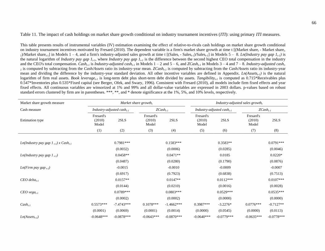
66
Table 11. The impact of cash holdings on market share growth conditional on industry tournament incentives (ITI): using primary ITI measures.
This table presents results of instrumental variables (IV) estimation examining the effect of relative-to-rivals cash holdings on market share growth conditional
on industry tournament incentives motivated by Fresard (2010). The dependent variable is a firm's market share growth at time t [(Market sharet - Market sharet-
1)/Market sharet-1] in Models 1 – 4, and a firm's industry-adjusted sales growth at time t [(Salest - Salest-1)/Salest-1] in Models 5 – 8. Ln(Industry pay gap 1t-1) is
the natural logarithm of Industry pay gap 1t-1, where Industry pay gap 1t-1 is the difference between the second highest CEO total compensation in the industry
and the CEO's total compensation. Casht-1 is Industry-adjusted casht-1 in Models 1 – 2 and 5 – 6, and ZCasht-1 in Models 3 – 4 and 7 – 8. Industry-adjusted casht-
1 is computed by subtracting from the Cash/Assets ratio its industry-year mean. ZCasht-1 is computed by subtracting from the Cash/Assets ratio its industry-year
mean and dividing the difference by the industry-year standard deviation. All other incentive variables are defined in Appendix. Ln(Assetst-1) is the natural
logarithm of firm real assets. Book leveraget-1 is long-term debt plus short-term debt divided by assets. Tangibilityt-1 is computed as 0.715*Receivables plus
0.547*Inventories plus 0.535*Fixed capital (see Berger, Ofek, and Swary, 1996). Consistent with Fresard (2010), all models include firm fixed effects and year
fixed effects. All continuous variables are winsorized at 1% and 99% and all dollar-value variables are expressed in 2003 dollars. p-values based on robust
standard errors clustered by firm are in parentheses. ***, **, and * denote significance at the 1%, 5%, and 10% levels, respectively.
Market share growth measure Market share growtht Industry-adjusted sales growtht
Cash measure Industry-adjusted casht-1 ZCasht-1
Industry-adjusted casht-1 ZCasht-1
Estimation type
Fresard's
(2010)
Model
2SLS
Fresard's
(2010)
Model
2SLS
Fresard's
(2010)
Model
2SLS
Fresard's
(2010)
Model
2SLS
(1) (2) (3) (4) (5) (6) (7) (8)
Ln(Industry pay gap 1 t-1) x Casht-1
0.7981***
0.1583***
0.3583**
0.0791***
(0.0032)
(0.0006)
(0.0285)
(0.0046)
Ln(Industry pay gap 1 t-1)
0.0458**
0.0471**
0.0185
0.0220*
(0.0487)
(0.0280)
(0.1790)
(0.0876)
Ln(Firm pay gap t-1)
-0.0015
-0.0010
-0.0009
-0.0007
(0.6917)
(0.7923)
(0.6838)
(0.7513)
CEO deltat-1
0.0157**
0.0147**
0.0112***
0.0107***
(0.0144)
(0.0210)
(0.0016)
(0.0028)
CEO vegat-1
0.0789***
0.0803***
0.0529***
0.0535***
(0.0002)
(0.0002)
(0.0000)
(0.0000)
Casht-1 0.5573*** -7.4743***
0.1078*** -1.4662***
0.3987*** -3.2276*
0.0776*** -0.7127**
(0.0001) (0.0069)
(0.0001) (0.0014)
(0.0000) (0.0545)
(0.0000) (0.0113)
Ln(Assetst-1) -0.0648*** -0.0878***
-0.0643*** -0.0870***
-0.0640*** -0.0779***
-0.0635*** -0.0778***

67
(0.0000) (0.0000)
(0.0000) (0.0000)
(0.0000) (0.0000)
(0.0000) (0.0000)
Book leveraget-1 0.2407*** 0.2511***
0.2523*** 0.2578***
0.1437*** 0.1574***
0.1519*** 0.1622***
(0.0000) (0.0000)
(0.0000) (0.0000)
(0.0000) (0.0000)
(0.0000) (0.0000)
Book leveraget-2 -0.1829*** -0.1706***
-0.1883*** -0.1794***
-0.1334*** -0.1355***
-0.1373*** -0.1411***
(0.0000) (0.0004)
(0.0000) (0.0001)
(0.0000) (0.0000)
(0.0000) (0.0000)
Market share growtht-1 -0.0659*** -0.0767***
-0.0655*** -0.0755***
(0.0000) (0.0000)
(0.0000) (0.0000)
Market share growtht-2 -0.0585*** -0.0661***
-0.0582*** -0.0674***
(0.0000) (0.0000)
(0.0000) (0.0000)
Industry-adjusted sales growtht-1
0.0809*** 0.0694***
0.0811*** 0.0699***
(0.0000) (0.0000)
(0.0000) (0.0000)
Industry-adjusted sales growtht-2
-0.0579*** -0.0661***
-0.0592*** -0.0670***
(0.0000) (0.0000)
(0.0000) (0.0000)
Year Fixed Effects Yes Yes
Yes Yes
Yes Yes
Yes Yes
Firm Fixed Effects Yes Yes
Yes Yes
Yes Yes
Yes Yes
Number of Observations 16,996 16,175
16,996 16,175
17,087 16,266
17,087 16,262
Anderson-Rubin Wald F-statistic for joint
relevance 10.22***
10.22***
10.96***
10.96***
Hansen J-statistic
0.786
2.326
0.0565
0.530
Difference in Sargan-Hansen statistics (test
for endogeneity) 40.18***
36.12***
44.40***
40.74***
First-stage F-statistics:
Ln(Industry pay gap 1 t-1) x Casht-1
92.08***
141.47***
131.66***
149.40***
Ln(Industry pay gap 1 t-1) 17.72***
17.72***
18.31***
18.31***
Casht-1
117.57***
135.07***
127.81***
144.86***
Instruments used in IV (2SLS): Number of CEOs within each industryt-1 x Tangibilityt-1
Ln(Sum of CEO compensation within each industryt-1) x Tangibilityt-1
Number of CEOs within each industryt-1
Tangibilityt-1

68
Table 12. The impact of cash holdings on market share growth conditional on industry tournament incentives (ITI): Using
alternative ITI measures
This table presents results of instrumental variables (IV) estimation examining the effect of relative-to-rivals cash holdings on market
share growth conditional on industry tournament incentives motivated by Fresard (2010) using alternative ITI measures. The dependent
variable is a firm's market share growth at time t [(Market sharet - Market sharet-1)/Market sharet-1] in Panel A, and a firm's industry-
adjusted sales growth at time t [(Salest - Salest-1)/Salest-1] in Panel B. Casht-1 is Industry-adjusted casht-1 in Models 1 – 3, and ZCasht-1 in
Models 4 – 6. Industry-adjusted casht-1 is computed by subtracting from the Cash/Assets ratio its industry-year mean. ZCasht-1 is
computed by subtracting from the Cash/Assets ratio its industry-year mean and dividing the difference by the industry-year standard
deviation. Ln(Industry pay gap 2t-1) is the natural logarithm of Industry pay gap 2t-1, where Industry pay gap 2t-1 is the difference
between the highest CEO total compensation in the industry and the CEO's total compensation. Ln(Industry pay gap 3t-1) the natural
logarithm of Industry pay gap 3t-1, where Industry pay gap 3t-1 is the difference between the highest CEO total compensation in the
industry and size group and the CEO's total compensation. Ln(Industry pay gap 4t-1) the natural logarithm of Industry pay gap 4t-1, where
Industry pay gap 4t-1 is the difference between the total compensation of the CEO 50 percentile points higher in the distribution and the
CEO's total compensation and for a CEO above the median it is the difference between the maximal CEO compensation in the industry
and the CEO's total compensation. All other incentive variables are defined in the Appendix. The control variables include Ln(Firm pay
gapt-1), CEO deltat-1, CEO vegat-1, Ln(Assetst-1), Book leveraget-1, and Book leveraget-2. Tangibilityt-1 is computed as 0.715*Receivables
plus 0.547*Inventories plus 0.535*Fixed capital (see Berger, Ofek, and Swary, 1996). Consistent with Fresard (2010), all models
include firm fixed effects and year fixed effects. All continuous variables are winsorized at 1% and 99% and all dollar-value variables
are expressed in 2003 dollars. p-values based on robust standard errors clustered by firm are in parentheses. ***, **, and * denote
significance at the 1%, 5%, and 10% levels, respectively.
Panel A. Dependent variable is Market share growtht
Cash measure Industry-adjusted casht-1 ZCasht-1
(1) (2) (3) (4) (5) (6)
Ln(Industry pay gap t-1) x Casht-1 1.1415***
0.1910***
(0.0088)
(0.0009)
Ln(Industry pay gap 2t-1) 0.0726**
0.0571**
(0.0391)
(0.0217)
Ln(Industry pay gap 3t-1) x Casht-1
0.9031***
0.1896***
(0.0080)
(0.0014)
Ln(Industry pay gap 3t-1)
0.0497*
0.0474*
(0.0824)
(0.0617)
Ln(Industry pay gap 4 t-1) x Casht-1
0.8287**
0.1900**
(0.0256)
(0.0115)
Ln(Industry pay gap 4 t-1) 0.0410
0.0486
(0.2432)
(0.1813)
Casht-1 -11.5858** -8.0214** -7.2251**
-1.8993*** -1.6811*** -1.6628**
(0.0132) (0.0143) (0.0399)
(0.0018) (0.0028) (0.0176)
Market share growtht-1 -0.0756*** -0.0783*** -0.0732***
-0.0746*** -0.0803*** -0.0740***
(0.0000) (0.0000) (0.0000)
(0.0000) (0.0000) (0.0000)
Market share growtht-2 -0.0697*** -0.0546*** -0.0711***
-0.0697*** -0.0560*** -0.0704***
(0.0000) (0.0000) (0.0000)
(0.0000) (0.0000) (0.0000)
Controls Yes Yes Yes Yes Yes Yes
Year Fixed Effects Yes Yes Yes
Yes Yes Yes
Firm Fixed Effects Yes Yes Yes
Yes Yes Yes
Number of Observations 16,539 16,192 16,539
16,539 16,192 16,539
Anderson-Rubin Wald F-statistic for
joint relevance
10.44*** 10.20*** 10.44***
10.44*** 10.20*** 10.44***
Hansen J-statistic 0.794 0.249 1.977
2.552 1.321 3.796*
Difference in Sargan-Hansen 38.19*** 37.16*** 37.70***
32.66*** 32.45*** 31.26***

69
statistics (test for endogeneity)
First-stage F-statistics:
Ln(Industry pay gap t-1) x Casht-1 125.65*** 121.52*** 119.78***
143.65*** 138.85*** 139.87***
Ln(Industry pay gap t-1) 20.60*** 45.59*** 12.80***
20.60*** 45.59*** 12.80***
Casht-1 120.40*** 116.42*** 120.40***
138.08*** 133.46*** 138.08***
Instruments used in IV (2SLS): Number of CEOs within each industryt-1 x Tangibilityt-1
Ln(Sum of CEO compensation within each industry t-1) x Tangibilityt-1
Number of CEOs within each industryt-1
Tangibilityt-1
Panel B. Dependent variable is Industry-adjusted sales growtht-1
Cash measure Industry-adjusted casht-1 ZCasht-1
(1) (2) (3) (4) (5) (6)
Ln(Industry pay gap 2t-1) x Casht-1 0.4489*
0.0896***
(0.0505)
(0.0080)
Ln(Industry pay gap 2t-1) 0.0225
0.0217
(0.2084)
(0.1275)
Ln(Industry pay gap 3t-1) x Casht-1
0.3729**
0.0904***
(0.0474)
(0.0081)
Ln(Industry pay gap 3t-1)
0.0168
0.0196
(0.2741)
(0.1682)
Ln(Industry pay gap 4t-1) x Casht-1
0.3551*
0.0915**
(0.0707)
(0.0201)
Ln(Industry pay gap 4t-1) 0.0100
0.0163
(0.5832)
(0.3940)
Casht-1 -4.3864* -3.1629* -2.9469
-0.8656** -0.7798** -0.7773**
(0.0764) (0.0820) (0.1165)
(0.0157) (0.0165) (0.0357)
Industry-adjusted sales growtht-1 0.0705*** 0.0679*** 0.0704***
0.0706*** 0.0667*** 0.0700***
(0.0000) (0.0000) (0.0000)
(0.0000) (0.0001) (0.0000)
Industry-adjusted sales growtht-2 -0.0699*** -0.0593*** -0.0732***
-0.0693*** -0.0597*** -0.0736***
(0.0000) (0.0000) (0.0000)
(0.0000) (0.0000) (0.0000)
Controls Yes Yes Yes Yes Yes Yes
Year Fixed Effects Yes Yes Yes
Yes Yes Yes
Firm Fixed Effects Yes Yes Yes
Yes Yes Yes
Number of Observations 16,627 16,274 16,627
16,627 16,274 16,627
Anderson-Rubin Wald F-statistic for
joint relevance
11.61*** 11.32*** 11.61***
11.61*** 11.32*** 11.61***
Hansen J-statistic 0.0114 0.00183 0.200
0.394 0.210 0.909
Difference in Sargan-Hansen
statistics (test for endogeneity) 45.57*** 43.80*** 46.37***
42.15*** 40.11*** 41.84***
First-stage F-statistics:
Ln(Industry pay gapt-1) x Casht-1 135.57*** 130.90*** 129.19***
153.16*** 147.82*** 149.50***
Ln(Industry pay gapt-1) 21.40*** 48.66*** 13.68***
21.40*** 48.66*** 13.68***
Casht-1 131.59*** 126.63*** 131.59***
149.07*** 143.43*** 149.07***
Instruments used in IV (2SLS): Number of CEOs within each industryt-1 x Tangibilityt-1
Ln(Sum of CEO compensation within each industryt-1) x Tangibilityt-1
Number of CEOs within each industryt-1
Tangibilityt-1

70
Fig. 1. Accumulation and dissipation of excess cash. This figure shows the change in excess cash
for the median firm over time. All firms with positive excess cash based on Table 8 (Model 9) are
included. The year with positive excess cash is considered year 0. The ratio plotted is the amount
of excess cash in year t divided by the amount of excess cash in year 0. Industry tournament
incentive (ITI) is measured as the difference between the second highest CEO total compensation
in the industry and the CEO's total compensation (Industry pay gap 1). ITI Q4 is the top quartile,
while Q1 is the bottom quartile.
0%
20%
40%
60%
80%
100%
120%
-4 -3 -2 -1 0 1 2 3 4
Year
% of Excess Cash Before or After t Years (Industry Tournament Incentive Quartiles)
ITI Q1
ITI Q2
ITI Q3
ITI Q4