Full Terms & Conditions of access and use can be found athttp://www.tandfonline.com/action/journalInformation?journalCode=fjds20

The Journal of Development Studies

ISSN: 0022-0388 (Print) 1743-9140 (Online) Journal homepage: http://www.tandfonline.com/loi/fjds20

Inequality of Opportunities at Early Ages: Evidencefrom Chile

Dante Contreras & Esteban Puentes

To cite this article: Dante Contreras & Esteban Puentes (2017) Inequality of Opportunities atEarly Ages: Evidence from Chile, The Journal of Development Studies, 53:10, 1748-1764, DOI:10.1080/00220388.2016.1262025

To link to this article: https://doi.org/10.1080/00220388.2016.1262025

View supplementary material

Published online: 08 Dec 2016.

Submit your article to this journal

Article views: 143

View related articles

View Crossmark data

Inequality of Opportunities at Early Ages:Evidence from Chile

DANTE CONTRERAS* & ESTEBAN PUENTES**Faculty of Economics and Business, Department of Economics, Universidad de Chile, Santiago, Chile

(Original version submitted October 2015; final version accepted November 2016)

ABSTRACT This paper examines inequality of opportunity for Chilean children starting from an early age. Ituses a psychometric test designed to assess children’s receptive vocabulary (PPVT), height, and weight asopportunity measures. We consider traditional circumstances such as parental income and educational level, butimprove on the previous literature including mother’s cognitive skills in our assessment. Our results indicate thatChilean children do not exhibit significant differences in height or weight either as newborns or at two tofour years old. Nevertheless, there is evidence of inequality of opportunities for vocabulary skills. Maternalcognitive ability is the greatest contributor. Finally, the evidence also suggests that inequality of opportunity onvocabulary skills increases with age.

1. Introduction

There is a recent and growing literature that studies inequality of opportunity. The original approachdeveloped by John Roemer has been translated into different methodologies that relate variables at theindividual level, such as personal income or achievement in academic measurement tests, with hisexogenous circumstances. These methodologies have been proposed by Bourguignon, Ferreira, andWalton (2007) and Checchi and Peragine (2010), and were later expanded on by Paes de Barros (2009)and Ferreira and Gignoux (2011). Several indicators have been constructed that calculate the level ofinequality of opportunities for different countries, allowing comparisons over time and across coun-tries. These studies have focused on examining the inequality on wages, educational performance, andaccess to basic services (drinking water, electricity, and sewage). However, the literature falls shortwhen it comes to examining the inequality at early ages, especially for health outcomes and cognitivedevelopment.

This is particularly relevant when we consider the vast empirical evidence that suggests theimportance of opportunities for young children. On one hand, health outcomes such as height andweight have been shown to be important predictors of outcomes in adolescence and adulthood(Grantham-McGregor et al., 2007). Also, cognitive ability measured at early ages is highly correlatedwith educational outcomes such as college attendance and returns to schooling (Heckman & Carneiro,2003). Additionally, early interventions that seek to improve health outcomes or cognitive develop-ment have long-term results on variables such as schooling, employment, and wages (Maluccio et al.,2009; Hoddinott, Maluccio, Behrman, Flores, & Martorell, 2008; and Gertler et al., 2014).Consequently, it is critical to study the level and evolution of young children’s opportunities.

Correspondence Address: Esteban Puentes, Faculty of Economics and Business, Department of Economics, Universidad deChile, Diagonal Paraguay 257, Of. 1603, Santiago, Chile. Email: epuentes@fen.uchile.clAn Online Appendix is available for this article which can be accessed through the online version of this journal available athttp://dx.doi.org/10.1080/00220388.2016.1262025

The Journal of Development Studies, 2017Vol. 53, No. 10, 1748–1764, https://doi.org/10.1080/00220388.2016.1262025

© 2016 Informa UK Limited, trading as Taylor & Francis Group

Previous evidence has found that Latin America has a high level of inequality of opportunities foradolescents, Ferreira and Gignoux (2014) perform a comparative study of students who took theProgramme of International Student Assessment or PISA test, and they find that inequality seems to behigher in Latin American countries and parts of continental Europe. Related to the research on equalityof opportunities, several papers have focused on estimating the relationship of the household’s socio-economic status and child outcomes, also finding that Latin America tends to exhibit greater inequal-ity. For instance, using data from Ethiopia, Peru, India, and Vietnam, López Bóo (2013) finds thatfrom ages five to eight, the relevance of socio-economic background seems to decrease for cognitiveskills, at the same time Peru stands out as a the country with the largest socio-economic gaps.Similarly, Schady et al. (2015) study the wealth gradient of children’s cognitive skills in Chile,Colombia, Ecuador, Nicaragua, and Peru; they find that there are important gaps by wealth and thatentering school does not seem to reduce the gaps. For Chile however, there is evidence of animprovement in equality of opportunities for young children. Contreras, Larranaga, Puentes, andRau (2012) find that from 1990 to 2006, the equality of opportunities improved for children betweenzero and five years of age for the following variables: access to preschool, good nutrition and water,and sanitation. Nonetheless, our paper contributes with evidence regarding the inequality of opportu-nities for variables more closely related to the quality of the provision of health and educationalservices than simple access.

Following the methodology presented in Ferreira and Gignoux (2014), this paper contributes newevidence regarding the measurement of inequality of opportunity for three aspects. First, it showsevidence of the inequality of opportunities at an early age (two to four years old). Second, it examinesthe degree of inequality of opportunity using health and cognitive variables as opportunities. In thecase of health, we use height and weight at birth and height and weight from two to four years old, andfor cognitive variables we use a vocabulary test (the PPVT). Finally, we control for a number of factorstraditionally ignored in the literature, which prove to be significant when it comes to explaininginequality. Specifically, mother’s cognitive skills, measured through the Wechsler Adults IntelligenceScale (WAIS) test, are a key factor in inequality of opportunities.

The evidence suggests that in Chile, newborns do not have significant differences in height orweight regardless of socioeconomic background. In other words, anthropometric outcomes are thesame for all children no matter their original socioeconomic background. However, there is evidencethat inequality of opportunity represents 17 per cent of the inequality observed in children’s cognitivetest performance. This measurement of inequality rises significantly with age. Upon deconstructingthis index of inequality of opportunity, maternal cognitive ability is the greatest contributor toinequality. Variables such as the presence of durable goods and parental education levels also havea significant impact.

This paper is divided into five sections. First is this introduction, Section 2 presents the data used inthis paper. Section 3 describes the methodology used in the paper. Section 4 discusses the results, andSection 5 presents the conclusions.

2. Data

This study uses the first round of the 2010 Early Childhood Longitudinal Survey (ELPI for itsacronym in Spanish). It includes data on 11,175 children born between 1 January 2006 and 31August 2009. It consisted of questionnaires from two household visits. The first visit was a socio-demographic household survey. On the second visit, several instruments were used to assess thecognitive, social-emotional, and physical development of the child. The survey is nationally repre-sentative for households with children five years old and younger.

An important aspect of the survey is that it not only uses data about the circumstances typically usedin inequality of opportunity literature such as household income, durable products in the home,ethnicity, and parental education, it also includes measures such as maternal cognitive ability throughthe use of the WAIS test.

Inequality of opportunities at early ages 1749

We focus on three different outcomes: height, weight, and a vocabulary test. The survey providesinformation on birth and current height and weight. We restrict the sample to children between 30 to60 months of age because the vocabulary test was only given to that sub-group.1 The final sampleconsists of 6114 children.

2.1. Main outcomes: Peabody picture vocabulary test (PPVT), height, and weight

The PPVT is a psychometric test designed to assess children’s receptive vocabulary; the internationalversion has been translated into Spanish (Test de Vocabulario en Imágenes Peabody o TVIP). Theinstrument is given to children between 2.5 and 5 years old. The test contains 125 laminated sheets,each of which contains four pictures. The examiner says a word and then asks the child to identify thepicture that best corresponds to the word.

The PPTV has been used for different goals such as proving the level of vocabulary accuracy atcertain ages, estimating the child’s scholastic aptitude, and longitudinal studies that measured changesin vocabulary accuracy over time. Importantly, the PPVT has predictive power over several relevantoutcomes during childhood and adulthood, such as wages (Schady et al., 2015).

The standardised scores are scaled from 55 to 145 points. Less than 96 points is a low score, whilescores between 96 and 103 points are average. Finally, scores above 103 are high scores (Dunn,Padilla, Lugo, & Dunn, 1986).

The survey also collects information about current and birth height and weight. In the case ofcurrent health outcomes, the enumerator measures the children, while the mother provides birth data.

A first approach to measure inequality of opportunity is to compare these indicators by incomelevel. We present the results using the absolute measure of each opportunity in the left graph, and thestandardised variable in the right. Figure 1 shows birth height of children in Chile by income quintile.On average, children born in 2009 are 49.6 centimetres tall. From the figure we observe that height ishighly independent of socioeconomic background. A similar pattern is observed for birth weight inFigure 2. The children weighed 3368 grammes at birth on average. Again, there are very smallsocioeconomic differences in this outcome.2 Thus, according to Figures 1 and 2, Chilean children havesimilar conditions at birth for anthropometric outcomes. This is quite a surprising result considering

Figure 1. Average newborn height by income quintile.

1750 D. Contreras & E. Puentes

the high levels of income inequality in Chile. One plausible explanation for these results is the publichealth policies that started in the 1920s and were greatly expanded during the 1970s. In 1924 Chilestarted a programme to provide milk for the children of working mothers and in 1937 the passage ofthe ‘Mother-Child Law’ initiated a plan of public health policies aimed at reducing risk duringpregnancy through periodic medical checks at community health centres.3 These policies wereaccompanied with a food intervention that provided half a litre of milk for children. While thesepolicies were ambitious, their coverage was low, reaching no more than 5 per cent of children by the1940s. It was in 1970, after Salvador Allende was elected, that this programme increased its reach toalmost 60 per cent of the children below 15 years of age and 54 per cent of pregnant women (Hakim &Solimano, 1976).4 While there are no studies that provide a causal link between these policies andhealth outcomes, other studies have argued that past health policies (since 1940) are associated withimprovements in health outcomes such as height (Nunez & Pérez, 2015). In addition, the Nunez andPérez (2015) provide evidence indicating the gap in height between individuals from different socio-economic groups is decreasing over time, which is consistent with a positive effect of the nutritionalpolicies. Nowadays, Chile exhibits some health outcomes that are comparable or better than otherOECD nations, for instance the percentage of low birth weight in Chile is 6 per cent, lower than the6.7 per cent average for OECD countries in 2011.5

In contrast, Figure 3 shows the PPVT and standardised PPVT by household income quintile. Thefigure shows that there is significant inequality in vocabulary development, for instance children fromthe richest families are 0.7 standard deviations above children from the poorest families.6 In addition,as we show in Section 4, that gap increases with age. Using a different data set, we also found thatsimilar differences are present for older children; at fourth grade the differences in test scores betweenthe poorest and richest quintile is 0.8 in math scores and 0.7 in language ones, and by tenth grades thegap increases to 1.2 standard deviations in math and 0.9 in language.7 These results suggest that thedifferences found in Ferreira and Gignoux (2014) at age 15 can be in part already explained bydifferences before age six.

Figure 2. Average newborn weight by income quintile.

Inequality of opportunities at early ages 1751

2.2. Circumstances: household characteristics

The ELPI allows us to construct several important variables that can be considered householdcircumstances. The previous literature mainly focuses on parents’ education, per capita income,gender, ethnicity and household durables. We include all those variables, but more importantly weinclude maternal cognitive ability, which has not been included in the previous literature.

As the measure of cognitive skills we use the Wechsler Adults Intelligence Scale (WAIS). TheWAIS is designed to measure global intelligence of individuals between 16 and 64 years old,regardless of education, socio-economic status, or reading level. It involves the application of twoscales, vocabulary and numeracy, comparing the results to the average scores obtained by subjects ofthe same age. The WAIS has been shown to have high measurement quality and predictive capacity onthe future behaviour of an individual; on the other hand, it needs to be updated approximately every 10years to offset to so-called ‘Flynn effect’ – the increase in IQ over time seen in most countries.

The WAIS test was given to the mothers as two subtests. The first subtest is a digit span thatassesses working memory, processing speed, and short-term auditory memory. A high score impliesrapid adaptation to the stimuli demands and flexibility of cognitive adaptation. The second subtest isthe vocabulary subtest that tests the ability to receive new information, store and use it properly. Thetest scale for each subset ranges from 0 to 19 points (Apfelbeck & Hermosilla, 2000).

As mentioned above we include parental education and occupation and per-capita income ascircumstances. As a measure of wealth, we also include information about durable goods. We considernumber of siblings as a measure of circumstances because it limits the available resources for anyspecific child in the household. Geographical zones help us to control for differences in the provisionof public services. We also include whether the child is a member of an ethnic group as a measure ofdifferentiated access to public services, labour markets, and general potential discrimination.

Table 1 shows the descriptive statistics for the entire sample and then by child age. We observe that16 per cent of the sample have mothers with primary education, 57 per cent of mothers have a

Figure 3. Vocabulary development by income quintile.

1752 D. Contreras & E. Puentes

secondary education, and 14 per cent have a college education. Meanwhile 11 per cent of the fathersare self-employed, and 8 per cent of the children belong to an ethnic group. The average per-capitahousehold income is $115,900 Chilean pesos, equivalent to US $200. Most of the households own arefrigerator (93%), but only 23 per cent own a laptop. There are no differences in circumstances bychild age.

3. Methodology

This section closely follows Ferreira and Gignoux (2014), which presents and discusses the construc-tion of inequality of opportunity indexes that are robust to standardisation of the outcome variablesunder study. They focus on the academic achievement of 15 year-olds using PISA test scores, whichare standardised and compared across countries.

They extend the methodology proposed by Bourguignon et al. (2007) and Ferreira and Gignoux(2011). Additionally, they build on Roemer (2009), which states that observed results depend on twofactors, the effort (E) of an individual, and his or her life circumstances (C) such as household incomeand parental education. Given that we are interested in inequality of opportunities at early ages, the

Table 1. Sample statistics

WholeSample 2 Years 3 Years 4 Years

Mean SD Mean SD Mean SD Mean SD

PPVT Score 106 15.19 104.3 11.54 106 16.06 108.2 16.97Weight (Grammes) 16503 3621 14830 2678 16641 3571 18503 3803Height (Centimeters) 98.81 6.60 93.34 5.13 99.49 5.49 104.70 4.97Male = 1 0.50 0.50 0.50 0.50 0.50 0.50 0.49 0.50Mother without formal education of unknown = 1 0.01 0.10 0.01 0.10 0.01 0.11 0.01 0.10Mother with primary education = 1 0.16 0.37 0.15 0.35 0.16 0.37 0.18 0.38Mother with secondary education = 1 0.57 0.50 0.57 0.50 0.57 0.50 0.55 0.50Mother with vocational education = 1 0.13 0.33 0.13 0.33 0.13 0.34 0.12 0.33Mother with college education = 1 0.14 0.34 0.15 0.36 0.13 0.33 0.14 0.35Father without formal education of unknown = 1 0.07 0.26 0.07 0.25 0.08 0.27 0.08 0.27Father with primary education = 1 0.15 0.36 0.14 0.35 0.16 0.37 0.16 0.37Father with secondary education = 1 0.53 0.50 0.54 0.50 0.53 0.50 0.50 0.50Father with vocational education = 1 0.10 0.30 0.10 0.30 0.11 0.31 0.08 0.28Father with college education = 1 0.15 0.35 0.16 0.37 0.13 0.33 0.17 0.38Father Self-Employed = = 1 0.11 0.31 0.10 0.30 0.10 0.31 0.13 0.33Ethnicity = 1 0.08 0.27 0.07 0.26 0.08 0.27 0.07 0.26Urban = 1 0.91 0.29 0.92 0.27 0.91 0.29 0.90 0.31Per-Capita HH Income 1.16 1.53 1.24 1.70 1.14 1.55 1.11 1.21Father Employment Unknown = 1 0.31 0.46 0.31 0.46 0.32 0.47 0.30 0.46Refrigerator = 1 0.93 0.25 0.93 0.25 0.93 0.26 0.94 0.23Washing machine = 1 0.78 0.42 0.78 0.42 0.77 0.42 0.80 0.40Microwave = 1 0.55 0.50 0.56 0.50 0.55 0.50 0.56 0.50Laptop = 1 0.23 0.42 0.22 0.42 0.23 0.42 0.25 0.43TV cable = 1 0.46 0.50 0.45 0.50 0.47 0.50 0.46 0.50Number of Siblings 0.99 1.00 0.93 1.00 0.99 1.00 1.08 0.99Maternal WAIS score (numeracy) 6.97 2.94 7.05 2.90 6.91 2.90 6.99 3.10Maternal WAIS score (vocabulary) 8.41 3.70 8.44 3.76 8.36 3.66 8.52 3.71Number of Observations 6114 1700 3219 1195

Notes: Per-capita household income in 100,000 s of 2010 Chilean peso. Average exchange rate during 2010 was501 Chilean pesos per US dollar.Source: ELPI 2010.

Inequality of opportunities at early ages 1753

effort component is much less important.8 Thus, the test scores can be expressed as a function ofcircumstances and a random or chance factor μð Þ:

score ¼ g C; μð Þ (1)

Finally, assuming linearity, the observed result can be expressed as a linear relationship with thecircumstances and a random factor:

scorei ¼ C0iθ þ �i (2)

Ferreira and Gignoux (2014) show that several inequality indexes such as the Generalized Entropy andGini coefficient are not equivalent before and after standardising the outcome variable, which leadsthem to use the variance, which is ordinally invariant to standardisation. Thus they propose thefollowing index of inequality of opportunities:

DIOp ¼ VarðC 0ibθÞ

Var scoreið Þ (3)

Where θ̂ corresponds to the OLS estimators of Equation (2).The use of the variance has several complications. It increases with the mean and does not hold the

transfer sensibility axiom, however, it is additively decomposable. Moreover, the index proposed byFerreira and Gignoux (2014) corresponds to an R-squared of the linear relationship between theoutcome variable and the set of circumstances (Equation [2] ).

Additionally, the linear approximation can be decomposed as follows:

θ̂IOp ¼Xj

θ̂j ¼Xj

Var scoreð Þ�1 θ̂2j var Cj þ 2Xk

θ̂k θ̂jcov CkCj

� �" #con j � k (4)

This decomposition allows us to calculate the contribution of each circumstance to total inequality;however as Ferreira and Gignoux (2014) point out, the decomposition is sensible to the specificationof Equation (2) and the number of circumstances included.

In the general specification there could be some omission of relevant variables, then the contributionof each circumstance would be contaminated by the correlation between the omitted variable and thecircumstance. In the Online Appendix we add maternal health variables as a set of circumstances. Ourresults are robust to the inclusion of these variables.9

In terms of the mechanisms that could explain how family characteristics and parental ability affectchildren behaviour, Duncan, Kalil, Mayer, Tepper, and Payne (2005) propose several ways that couldexplain the positive correlations between parents and children’s traits that have been largely found inthe literature. They state and test four mechanisms for the transmission of traits: genetic, socio-economic status, role-models, and parenting style. In the case of the genetic mechanism, abilitiesand other traits are simply inherited. The socio-economic mechanism basically states that parents withhigher abilities tend to have a higher income, and are then able to provide more and better inputs fortheir children’s ability production function. Good parenting styles such as involvement, control,emotional warmth, and cognitive stimulation could also have a positive effect on many children’soutcomes including ability, and more able parents could in general be more likely to adopt these goodparenting styles. Finally, the role-model mechanism assumes that children mimic the behaviour of theirparents; it is more likely to explain the transmission of social behaviour than cognitive skills. Theauthors find some evidence in favour of the genetic and role model mechanisms for several beha-vioural and cognitive traits.

1754 D. Contreras & E. Puentes

4. Results

In this section we present the results from several models of Equation (2). First, we evaluate the importanceof including the maternal WAIS test in calculating the effects of inequality of opportunity on a child’svocabulary development. At the same time, we compare this inequality with birth height and weight inTable 2. A second set of calculations is done for different age groups, which examine whether inequality of

Table 2. OLS estimation, whole sample

VARIABLES PPVT PPVT Weight at birth Height at birth

Male = 1 −0.065** −0.067*** 0.137*** 0.202***(0.026) (0.025) (0.026) (0.027)

Mother without formal education of unknown = 1 0.069 0.102 −0.027 −0.097(0.123) (0.126) (0.121) (0.114)

Mother with primary education = 1 −0.155*** −0.022 0.045 0.043(0.036) (0.036) (0.041) (0.043)

Mother with vocational education = 1 0.152*** 0.078* −0.065 −0.004(0.048) (0.047) (0.042) (0.048)

Mother with college education = 1 0.345*** 0.214*** −0.073 −0.069(0.053) (0.052) (0.051) (0.054)

Father without formal education of unknown = 1 −0.046 −0.040 −0.121** −0.087(0.052) (0.050) (0.055) (0.054)

Father with primary education = 1 −0.185*** −0.165*** 0.003 −0.012(0.036) (0.035) (0.040) (0.040)

Father with vocational education = 1 0.115** 0.103** −0.049 −0.035(0.051) (0.048) (0.048) (0.048)

Father with college education = 1 0.076 0.023 0.012 0.041(0.052) (0.051) (0.048) (0.053)

Father Self-Employed = = 1 0.047 0.040 0.026 0.044(0.043) (0.042) (0.046) (0.044)

Ethnicity = 1 −0.158*** −0.120*** 0.054 −0.003(0.042) (0.041) (0.047) (0.052)

Urban = 1 0.126*** 0.109*** −0.004 −0.015(0.040) (0.039) (0.045) (0.044)

Per-Capita HH Income 0.021 0.012 −0.015 −0.022*(0.014) (0.012) (0.012) (0.012)

Father Employment Unknown = 1 −0.112*** −0.106*** −0.066** −0.021(0.030) (0.029) (0.031) (0.031)

Refrigerator = 1 0.096** 0.086* −0.044 0.044(0.047) (0.046) (0.054) (0.053)

Washing machine = 1 0.069** 0.031 0.071** 0.032(0.031) (0.031) (0.035) (0.035)

Microwave = 1 0.081*** 0.066** −0.054* −0.028(0.027) (0.027) (0.028) (0.028)

Laptop = 1 0.126*** 0.095** −0.085** −0.046(0.042) (0.041) (0.038) (0.044)

TV cable = 1 0.224*** 0.216*** 0.012 0.032(0.027) (0.027) (0.028) (0.029)

Number of Siblings −0.080*** −0.088*** 0.048*** 0.023(0.014) (0.013) (0.014) (0.015)

Maternal WAIS subset numeracy 0.036*** −0.001 0.005(0.005) (0.005) (0.005)

Maternal WAIS subset vocabulary 0.040*** −0.000 −0.000(0.004) (0.004) (0.004)

Constant −0.310*** −0.803*** −0.029 −0.154*(0.065) (0.072) (0.082) (0.084)

Observations 6,114 6,114 6,114 6,114R-squared 0.139 0.173 0.019 0.016

Notes: Robust standard errors in parentheses. *** p < 0.01, ** p < 0.05, * p < 0.1.

Inequality of opportunities at early ages 1755

opportunity increases over time.We calculate these changes for vocabulary development and child’s heightandweight from two to four years old. These results are presented in Tables 3–5. To statistically evaluate thedifferences among the inequality of opportunity, we calculate confidence intervals for the R-squared. Wecalculate bootstrap confidence intervals using 999 repetitions and adjusting for bootstrap bias (adjusted

Table 3. OLS estimations, Two year-old

VARIABLES PPVT Weight (Grammes) Height (Cms)

Male = 1 −0.016 0.129*** 0.169***(0.038) (0.035) (0.039)

Mother without formal education of unknown = 1 −0.089 −0.209 −0.390(0.131) (0.260) (0.292)

Mother with primary education = 1 −0.043 0.089 −0.031(0.049) (0.055) (0.066)

Mother with vocational education = 1 0.049 0.020 −0.006(0.071) (0.053) (0.059)

Mother with college education = 1 0.239*** 0.052 0.076(0.081) (0.058) (0.072)

Father without formal education of unknown = 1 −0.039 −0.034 0.076(0.071) (0.083) (0.093)

Father with primary education = 1 −0.004 0.015 0.065(0.051) (0.055) (0.058)

Father with vocational education = 1 0.194*** −0.069 0.013(0.072) (0.066) (0.074)

Father with college education = 1 0.010 −0.069 0.120(0.077) (0.060) (0.074)

Father Self-Employed = = 1 0.080 −0.055 −0.011(0.071) (0.061) (0.064)

Ethnicity = 1 −0.005 −0.014 −0.065(0.060) (0.053) (0.078)

Urban = 1 0.069 0.144* −0.063(0.055) (0.077) (0.066)

Per-Capita HH Income 0.005 0.001 −0.004(0.015) (0.012) (0.016)

Father Employment Unknown = 1 −0.103** −0.001 −0.009(0.041) (0.042) (0.046)

Refrigerator = 1 0.045 −0.066 0.017(0.066) (0.077) (0.084)

Washing machine = 1 0.050 0.127*** 0.009(0.044) (0.049) (0.053)

Microwave = 1 0.024 −0.014 0.059(0.040) (0.039) (0.042)

Laptop = 1 0.034 −0.074* −0.040(0.060) (0.042) (0.059)

TV cable = 1 0.097** −0.005 0.083**(0.038) (0.037) (0.041)

Number of Siblings −0.097*** −0.025 −0.022(0.018) (0.018) (0.020)

Maternal WAIS subset numeracy 0.030*** −0.001 −0.016*(0.008) (0.007) (0.008)

Maternal WAIS subset vocabulary 0.015*** 0.004 0.006(0.006) (0.005) (0.007)

Constant −0.570*** −0.656*** −0.877***(0.100) (0.113) (0.118)

Observations 1,700 1,700 1700R-squared 0.127 0.022 0.031

Notes: Robust standard errors in parentheses. *** p < 0.01, ** p < 0.05, * p < 0.1.

1756 D. Contreras & E. Puentes

column) and not adjusting for bias (unadjusted column). The confidence intervals of the overall indexes,from Table 2, are presented in Table 6, while the confidence intervals of the indexes calculated by age, fromTables 3–5, are shown in Table 7. Finally, in Table 8 we calculate the contribution of each circumstance tooverall inequality of opportunities.

Table 4. OLS estimations three year-old

VARIABLES PPVT Weight (Grammes) Height (Cms.)

Male = 1 −0.060 0.137*** 0.211***(0.036) (0.034) (0.030)

Mother without formal education of unknown = 1 −0.010 −0.130 −0.151(0.183) (0.141) (0.154)

Mother with primary education = 1 −0.075 −0.022 0.035(0.051) (0.053) (0.044)

Mother with vocational education = 1 0.134** 0.135** 0.122**(0.065) (0.064) (0.050)

Mother with college education = 1 0.213*** −0.064 0.028(0.075) (0.066) (0.058)

Father without formal education of unknown = 1 −0.035 0.063 0.092(0.073) (0.062) (0.061)

Father with primary education = 1 −0.190*** 0.047 0.016(0.051) (0.050) (0.045)

Father with vocational education = 1 0.038 −0.136** −0.056(0.069) (0.066) (0.053)

Father with college education = 1 0.053 0.028 0.042(0.074) (0.063) (0.054)

Father Self-Employed = = 1 0.015 0.060 −0.027(0.061) (0.055) (0.046)

Ethnicity = 1 −0.138** −0.043 −0.029(0.057) (0.071) (0.049)

Urban = 1 0.115** 0.059 −0.064(0.057) (0.062) (0.052)

Per-Capita HH Income 0.018 0.001 0.008(0.018) (0.008) (0.012)

Father Employment Unknown = 1 −0.087** −0.042 0.016(0.043) (0.042) (0.035)

Refrigerator = 1 0.081 0.012 0.019(0.067) (0.067) (0.057)

Washing machine = 1 −0.049 0.057 0.108***(0.044) (0.043) (0.041)

Microwave = 1 0.083** −0.003 −0.008(0.038) (0.038) (0.033)

Laptop = 1 0.086 −0.004 −0.025(0.058) (0.047) (0.045)

TV cable = 1 0.258*** 0.032 0.015(0.039) (0.037) (0.033)

Number of Siblings −0.086*** −0.057*** −0.033**(0.019) (0.017) (0.016)

Maternal WAIS subset numeracy 0.037*** 0.008 0.011**(0.007) (0.006) (0.006)

Maternal WAIS subset vocabulary 0.048*** 0.007 0.010*(0.006) (0.005) (0.005)

Constant −0.830*** −0.204** −0.213**(0.103) (0.098) (0.095)

Observations 3,219 3,219 3,219R-squared 0.184 0.017 0.034

Notes: Robust standard errors in parentheses. *** p < 0.01, ** p < 0.05, * p < 0.1.

Inequality of opportunities at early ages 1757

As circumstance variables we include: parental education and occupation, per-capita householdincome, ethnicity, geographical zone, dummy variables for durable goods, number of siblings, and thematernal numeracy and vocabulary WAIS scores separately.

In Table 2 we observe that inequality of opportunity in vocabulary development is 17 per cent forthe entire population (when WAIS scores are included), while the inequality of opportunity index for

Table 5. OLS estimations four year-old

VARIABLES PPVT Current Weight Current Height

Male = 1 −0.113* 0.114* 0.128***(0.060) (0.060) (0.047)

Mother without formal education of unknown = 1 0.665** 0.640** 0.133(0.306) (0.290) (0.243)

Mother with primary education = 1 0.112 0.057 −0.110(0.090) (0.087) (0.076)

Mother with vocational education = 1 −0.005 −0.048 −0.044(0.102) (0.100) (0.080)

Mother with college education = 1 0.200* −0.056 0.051(0.115) (0.121) (0.085)

Father without formal education of unknown = 1 −0.110 −0.080 0.010(0.118) (0.119) (0.088)

Father with primary education = 1 −0.269*** −0.096 0.020(0.088) (0.095) (0.067)

Father with vocational education = 1 0.134 0.025 0.045(0.112) (0.109) (0.080)

Father with college education = 1 0.004 −0.091 0.008(0.105) (0.113) (0.080)

Father Self-Employed = = 1 0.031 0.011 0.033(0.095) (0.098) (0.072)

Ethnicity = 1 −0.195* 0.070 −0.064(0.115) (0.100) (0.079)

Urban = 1 0.165* 0.247** −0.065(0.092) (0.109) (0.062)

Per-Capita HH Income 0.073* 0.006 −0.021(0.042) (0.024) (0.024)

Father Employment Unknown = 1 −0.113 0.121 0.107**(0.072) (0.074) (0.054)

Refrigerator = 1 0.148 0.167 0.220**(0.124) (0.121) (0.105)

Washing machine = 1 0.226*** −0.076 0.046(0.081) (0.079) (0.060)

Microwave = 1 0.057 −0.037 −0.048(0.065) (0.063) (0.050)

Laptop = 1 0.096 0.078 0.126**(0.085) (0.080) (0.064)

TV cable = 1 0.243*** 0.014 0.114**(0.063) (0.066) (0.052)

Number of Siblings −0.076** −0.055* −0.008(0.032) (0.030) (0.026)

Maternal WAIS subset numeracy 0.038*** 0.004 0.002(0.011) (0.011) (0.008)

Maternal WAIS subset vocabulary 0.054*** 0.005 −0.002(0.010) (0.009) (0.007)

Constant −1.104*** 0.136 0.610***(0.185) (0.187) (0.134)

Observations 1,195 1,195 1,195R-squared 0.255 0.025 0.039

Notes: Robust standard errors in parentheses. *** p < 0.01, ** p < 0.05, * p < 0.1.

1758 D. Contreras & E. Puentes

birth height and weight is close to 2 per cent. These results confirm the evidence presented in Section 2where we see little difference in height and weight at birth by income quintile, but significantdifferences in vocabulary development by income. Additionally, we observe in Table 2 that inequalityof opportunity increases when we consider maternal cognitive measures from 14 per cent to 17 percent when maternal cognition is included in the model. Table 6 shows the confidence intervalscalculated by using bootstrapping for these indexes, which statistically confirms the higher degreeof inequality in vocabulary development than in birth measurements. The comparison between theconfidence intervals for child vocabulary development including maternal cognitive measures isstatistically significant at 5 per cent when we use bootstrap methodology that corrects for bias(adjusted column) and when we do not correct for bias (unadjusted column). Thus, we find thatincluding maternal cognitive skills increases the index of inequality of opportunities in 20 per cent.This is an important lesson, because it implies that to understand the degree of inequality ofopportunities for child outcomes, we should include parental characteristics that measure cognitiveability.

Table 6. PPVT inequality index, 95 per cent confidence intervals calculated using bootstrap (999 repetitions)

Not Including WAIS

Unadjusted Adjusted

PPVT PPVT

LB 0.125 0.122UP 0.159 0.152

Including WAIS

Unadjusted Adjusted Unadjusted Adjusted Unadjusted Adjusted

PPVT Height at Birth Weight at Birth

LB 0.160 0.156 0.013 0.009 0.016 0.013UP 0.193 0.188 0.026 0.019 0.030 0.022

Notes: LB: lower bound. UP: upper bound. Unadjusted: Confidence interval by percentile methodology. Adjusted:bootstrap bias corrected confidence interval.

Table 7. 95 per cent confidence intervals calculated using bootstrap, by age (999 repetitions)

2 years old 3 years old 4 years old

Unadjusted Adjusted Unadjusted Adjusted Unadjusted Adjusted

PPTVLB 0.107 0.091 0.167 0.158 0.225 0.197UP 0.171 0.146 0.213 0.204 0.311 0.284WeightLB 0.019 0.013 0.014 0.011 0.023 0.014UP 0.056 0.025 0.034 0.020 0.068 0.027HeightLB 0.028 0.023 0.028 0.021 0.036 0.021UP 0.067 0.036 0.055 0.041 0.081 0.042

Notes: LB: lower bound. UP: upper bound. Unadjusted: Confidence interval by percentile methodology. Adjusted:bootstrap bias corrected confidence interval.

Inequality of opportunities at early ages 1759

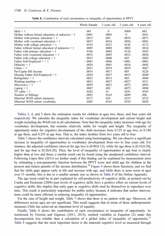
Tables 3, 4, and 5 show the estimation results for children at ages two, three, and four years oldrespectively. We calculate the inequality index for vocabulary development and current height andweight including the WAIS test in all calculations. Note that the inequality index increases with age forvocabulary development, but remains relatively stable for weight and height. The inequality ofopportunity index for cognitive development of the child increases from 0.125 at age two, to 0.186at age three, and 0.255 at age four. That is, the index doubles from two years old to four.

Table 7 shows the confidence intervals calculated using bootstrapping. We can observe a significantincrease in inequality of opportunities in vocabulary development from two to four years old. Forinstance, the adjusted confidence interval for age two is [0.09;0.15], while for age three is [0.16;0.20],and for age four is [0.20;0.28]. Then, the level of inequality of opportunities at age four is clearlyhigher than at two and three; a similar result can be found using the unadjusted confidence interval.Following López Bóo (2013) we further study if this finding can be explained by measurement errorby estimating a non-parametric function between the PPVT score and child age for children in thepoorest and richest quintile of the income distribution.10 Figure 4 shows these functions, and we findthat the skills gaps appear early in life and increase with age, and while there is more noise at agesover 51 months, this is due to a smaller sample size as shown in Table 8 of the Online Appendix.

The age trend could be in part explained by self-productivity of cognitive skills, as pointed out byCunha and Heckman (2008) past levels of cognitive skills have a positive effect on current levels ofcognitive skills; this implies that early gaps in cognitive skills tend by themselves to reproduce overtime. This result is particularly important for public policy because it indicates that earlier interven-tions could be more efficient in reducing inequality of opportunities.

For the case of height and weight, Table 7 shows that there is no pattern with age. Moreover, alldifferences across ages are not significant. This result suggests that in terms of these anthropometricmeasures Chile has achieved an important level of equality.

Finally, Table 8 shows the contribution of each circumstance to inequality of opportunity. Asmentioned by Ferreira and Gignoux (2011, 2014), omitted variables in Equation (2) make thisdecomposition less reliable than a calculation of a global index of inequality of opportunity.11

Table 8 suggests that the most important factor is the maternal cognitive level as measured through

Table 8. Contribution of each circumstance to inequality of opportunities in PPVT

Whole Sample 2 years old 3 years old 4 years old

Male = 1 .001 0 .0009 .003Mother without formal education of unknown = 1 −.0001 .0005 0 .0031Mother with primary education = 1 .0015 .003 .0052 −.0071Mother with vocational education = 1 .0027 .0016 .0056 −.0001Mother with college education = 1 .0165 .0251 .0142 .0172Father without formal education of unknown = 1 .0005 .0008 .0003 .0016Father with primary education = 1 .0106 .0002 .0126 .0203Father with vocational education = 1 .0032 .0085 .0012 .0028Father with college education = 1 .0015 .0008 .003 .0003Father Self-Employed = = 1 −.0001 .0006 −.0001 −.0001Ethnicity = 1 .0026 .0001 .0034 .0045Urban = 1 .0031 .0019 .0029 .0067Per-Capita HH Income .0035 .0017 .005 .0226Missing Father Self-Employed = 1 .0028 .0037 .0015 .0048Refrigerator = 1 .0023 .0012 .002 .0044Washing machine = 1 .0021 .0037 −.0027 .0211Microwave = 1 .0059 .0021 .0072 .0055Laptop = 1 .0087 .003 .0075 .0098TV cable = 1 .0242 .01 .0281 .0305Number of Siblings .0091 .0163 .0089 .006Maternal WAIS subset numeracy .0273 .026 .0253 .0322Maternal WAIS subset vocabulary .0445 .0163 .0524 .0656

1760 D. Contreras & E. Puentes

the WAIS test, with the vocabulary subset being more important. This can be explained because thePPVT also measures vocabulary skills, then there could be a direct transmission of vocabulary formmother to child. The importance of both components of the WAIS test also tends to increase with theage of the child. Additionally, household income also becomes more important as the child ages. Thisresult suggests that the effects of income inequality could start early in life with a strong intergenera-tional transmission of income, which has been documented in Urzua, Rodriguez, and Contreras(2014).

5. Conclusions

In this paper we analyse inequality of opportunities for young children. Using a unique dataset fromChile, we take advantage of several measures of children’s physical and cognitive development toassess the importance of circumstances. We also use detailed measures of maternal ability, whichallows us to obtain a better approximation of the level of inequality of opportunities.

We find that for the sample, traditional circumstances such as household income and parentaleducation explain 14 per cent of the variation in development of children between two and four yearsold. This increases to 17 per cent when considering maternal cognitive ability measures. These resultssuggest that inequality of opportunity that begins early in life is affected by maternal cognitive ability.Meanwhile, physical measures such as height and weight are much less likely to be affected inequalityof opportunities.

Additionally, we found that inequality of vocabulary development increases significantly from agetwo to four, indicating that not only is inequality important at an early age, but also becomesincreasingly important over time. Moreover, our results show similar gaps by income quintile infourth grade testing, suggesting that socio-economic gaps in school could start before formaleducation.

Figure 4. Age Patterns in PPVT, Local polynomial smooth estimator.Note: Nonparametric estimation of standardised PPVT on age by household per capita income. Bandwidth ischosen to minimise the conditional weighted mean integrated squared error. For the poorest quintile bandwidth is

1.7 and for the richest quintile is 2.1

Inequality of opportunities at early ages 1761

In terms of policies that could be implemented to reduce the inequality of opportunities in skills, ourresults indicate that maternal ability plays an important role. Public policies should not necessarilyfocus on improving maternal skills, but might be more efficient to provide all mothers, and especiallythose from more disadvantaged backgrounds, with tools to help them stimulate their children. Someinterventions in this vein have proved successful. For example, Attanasio, Fitzsimons, Grantham-McGregor, Douglas, and Rubo-Codina (2014) compared three interventions for children between 12 to24 months in Colombia. The first intervention consisted of psychosocial stimulation, the secondconsisted of increasing nutrient quality and the third was a combination of the first and second. Theauthors find that only the first intervention had a positive and large effect on cognitive scores.Importantly, the stimulation programme was delivered through the local community and at a lowcost, which could easily be replicated in other countries.

Also, free or cheap access to day-care centres could be useful to reduce skill gaps, although theevidence of this is mixed. Specifically, Noboa and Urzua (2012) find for Chile that public day-carecentres can at the same time improve child outcomes such as emotional regulation, but negativelyaffect others such as child-adult interactions. Thus it is important to consider not only coverage butalso quality of day-care policies.

Since research has found the importance of both cognitive and non-cognitive abilities in adulthood(Heckman, Stixrud, & Urzua, 2006), future research should focus on non-cognitive abilities. Thiscould be done in two ways: one is considering parental non-cognitive abilities as child circumstances,and the other is studying how circumstances affect children’s non-cognitive abilities.

Acknowledgment

We would like to thank Tomás Rau, Jaime Ruiz Tagle, and Patricia Medrano for their comments. Wethank Nicolás Campos for his valuable research assistance. This version of the paper has benefitedfrom comments made by two anonymous referees. Data and code will be available on request. DanteContreras also acknowledges funding from the Centre for Social Conflict and Cohesion Studies(CONICYT/FONDAP/15130009).

Disclosure statement

No potential conflict of interest was reported by the authors.

Funding

This work was supported by the Centre for Social Conflict and Cohesion Studies [CONICYT/FONDAP/15130009]; Comisión Nacional de Investigación Científica y Tecnológica [15130009];

Notes

1. We group children into three age categories: two, three, and four years of age, which correspond to children between 25 to30 months-old, between 36 to 47 months-old, and between 48 to 59 months-old respectively.

2. All means are not statistically different at 5 per cent, except for the means of children living in the richest households, whohave a slight lower height and weight than the rest of the population.

3. The minister of Health at the time, Eduardo Cruz Coke, was one of the most influential people promoting these policies(Hakim & Solimano, 1976).

4 For more details on those policies see Larrañaga (2010).5. OECD Family database: http://www.oecd.org/social/family/database.htm, accessed on 22 September 2015.6. The differences are statistically significant at 5 per cent.7. See Online Appendix, Table 10 A8. In the standard approach to measure inequality of opportunities (previously developed by Bourguignon et al. (2007) and

Ferreira and Gignoux (2011) both circumstances and effort play a role in explaining inequality of opportunities. In that

1762 D. Contreras & E. Puentes

model a person’s effort depending on the circumstances and a random factor or luck (ν) is expressed as E = h (C, v). In thepresent context, it is difficult to argue that effort plays a role for very young children. As a consequence of that we follow amodel based only on circumstances.

9. We excluded some variables because of a potential double causality problem such as maternal socio-emotional status,whether the mother was working and parenting techniques. If these variables are positively related to maternal cognitiveskills, we would be over-estimating the effect of mother’s skills or any other variable included in our specification

10. As mentioned before, we perform a robust analysis including more variables and the results are very similar. See Tables 1Ato 7A in the Online Appendix.

11. As mentioned before, we perform a robust analysis including more variables and the results are very similar. See Tables 1Ato 7A in the Online Appendix

References

Apfelbeck, E.-M., & Hermosilla, M. (2000). Manual de Administración y Tabulación del Test de WAIS. Santiago.Attanasio, O. P., Fitzsimons, E. O. A., Grantham-McGregor, S. M., Douglas, C. M., & Rubo-Codina, M. (2014). Using the

infrastructure of a conditional cash transfer program in Colombia: Cluster randomized controlled trial. British MedicalJournal, 349, g5785. doi:10.1136/bmj.g5785

Bourguignon, F., Ferreira, F. H., & Walton, M. (2007). Equity, efficiency and inequality traps: A research agenda. The Journal ofEconomic Inequality, 5(2), 235–256. doi:10.1007/s10888-006-9042-8

Checchi, D., & Peragine, V. (2010). Inequality of opportunity in Italy. The Journal of Economic Inequality, 8(4), 429–450.doi:10.1007/s10888-009-9118-3

Contreras, D., Larranaga, O., Puentes, E., & Rau, T. (2012). Chile: Evaluation of the opportunities for children, 1990-2006.CEPAL Review, (106), 115–133.

Cunha, F., & Heckman, J. J. (2008). Formulating, identifying and estimating the technology of cognitive and noncognitive skillformation. Journal of Human Resources, 43(4), 738–782. doi:10.1353/jhr.2008.0019

Duncan, G., Kalil, A., Mayer, S. E., Tepper, R., & Payne, M. R. (2005). The apple does not fall far from the tree. In S. Bowles,H. Gintis, M. Osborne Groves (Eds.), Unequal chances: Family background and economic success. New York, NY: RussellSage Foundation.

Dunn, L. M., Padilla, E. R., Lugo, D. E., & Dunn, L. M. (1986). Manual del Examinador para el Test de Vocabulario enImágenes Peabody: Adaptación Hispanoamericana (Peabody Picture Vocabulary Test: Hispanic-American Adaptation).Minnesota: AGS.

Ferreira, F. H., & Gignoux, J. (2011). The measurement of inequality of opportunity: Theory and an application to LatinAmerica. Review of Income and Wealth, 57(4), 622–657. doi:10.1111/j.1475-4991.2011.00467.x

Ferreira, F. H., & Gignoux, J. (2014). The measurement of educational inequality: Achievement and opportunity. The WorldBank Economic Review, 28(2), 210–246. doi:10.1093/wber/lht004

Grantham-McGregor, S., Cheung, Y. B., Cueto, S., Glewwe, P., Ritcher, L., & Strupp, B. (2007). Developmental potential in thefirst 5 years for children in developing countries. The Lancet, 369(9555), 60–70. doi:10.1016/S0140-6736(07)60032-4

Hakim, P., & Solimano, G. (1976). Supplemental feeding as a nutritional intervention: The chilean experience in the distributionof milk. Journal of Tropical Pediatrics, 22(4), 185–202. doi:10.1093/tropej/22.4.185

Heckman, J., & Carneiro, P. (2003). Human capital policy (No. w9495). National Bureau of Economic Research.Heckman, J. J., Stixrud, J., & Urzua, S. (2006). The effects of cognitive and noncognitive abilities on labor market outcomes and

social behavior. Journal of Labor Economics, 24(3), 411–482. doi:10.1086/504455Hoddinott, J. F., Maluccio, J. A., Behrman, J. R., Flores, R., & Martorell, R. (2008). Effect of a nutrition intervention during

early childhood on economic productivity in guatemalan adults. The Lancet, 371(9610), 411–416. doi:10.1016/S0140-6736(08)60205-6

Gertler, P., Heckman, J., Pinto, R., Zanolini, A., Vermeersch, C., Walker, S. . . . Grantham-McGregor, S. (2014). Labor marketreturns to an early childhood stimulation intervention in Jamaica. Science, 344(6187), 998–1001. doi:10.1126/science.1251178

Larrañaga, O. (2010). “El Estado Bienestar en Chile: 1910–2010.” In R. Lagos (Ed.), Cien Años de Luces y Sombras (Vol. 2).Santiago de Chile: Taurus.

López Bóo, F. (2013). Intercontinental evidence on socioeconomic status and early childhood: Cognitive skills: Is latin Americadifferent? (No. 81846). Inter-American Development Bank.

Maluccio, J. A., Hoddinott, J. F., Behrman, J. R., Quisumbing, A. R., Martorell, R., & Stein, A. D. (2009). The impact ofnutrition during early childhood on education among guatemalan adults. Economic Journal, 119(537), 734–763.doi:10.1111/j.1468-0297.2009.02220.x

Noboa-Hidalgo, G. E., & Urzua, S. S. (2012). The effects of participation in public child care centers: Evidence from Chile.Journal of Human Capital, 6(1), 1–34. doi:10.1086/664790

Nunez, J., & Pérez, G. (2015). Trends in physical stature across socioeconomic groups of Chilean boys, 1880–1997. Economics& Human Biology, 16, 100–114. doi:10.1016/j.ehb.2013.12.008

Paes De Barros, R. (2009). Measuring inequality of opportunities in Latin America and the Caribbean. World BankPublications.

Inequality of opportunities at early ages 1763

Roemer, J. E. (2009). Equality of opportunity. Harvard University Press.Schady, N., Behrman, J., Araujo, M. C., Azuero, R., Bernal, R., Bravo, D. . . . Vakis, R. (2015). Wealth gradients in early

childhood cognitive development in five Latin American countries. Journal of Human Resources, 50(2), 446–463.doi:10.3368/jhr.50.2.446

Urzua, S., Rodriguez, J., & Contreras, D. (2014). On the origins of inequality in Chile. Mimeo.

1764 D. Contreras & E. Puentes