inertial currents in the southern gulf of mexico ... · expósito-díaz et al.: inertial currents...

Ciencias Marinas (2009), 35(3): 287–296

287

Introduction

Ocean dynamics are characterized by processes that occur

at a variety of temporal scales, among them inertial or free

oscillations, which are prominent in some areas (e.g., Knauss

2000). Inertial oscillations may play a crucial role in pollution

transport (Pickett et al. 1984, Schumann et al. 2005) and

plankton fate (Pingree et al. 1982, Van Haren et al. 1999). For

instance, the Bay of Campeche, in the southern Gulf of Mexico

(fig. 1), is an area of major economic resources due to its

fisheries and large number of oil platforms in operation (Salas-

Introducción

La dinámica del océano se caracteriza por procesos que

ocurren en una amplia variedad de escalas temporales, entre

ellas la inercial o de las oscilaciones libres, que son importan-

tes en algunas regiones de los océanos (e.g., Knauss 2000). Las

oscilaciones inerciales pueden jugar un papel crucial en el

transporte de contaminantes (Pickett et al. 1984, Schumann et

al. 2005) y en la distribución del plancton (Pingree et al. 1982,

Van Haren et al. 1999). Por ejemplo, la Bahía de Campeche,

en el sur del Golfo de México (fig. 1), es un sitio con gran

Inertial currents in the southern Gulf of Mexico

Corrientes inerciales en el sur del Golfo de México

G Expósito-Díaz1, DA Salas-de León2*, MA Monreal-Gómez2, D Salas-Monreal3, F Vázquez-Gutiérrez2

1 Posgrado en Ciencias del Mar y Limnología, Universidad Nacional Autónoma de México, Circuito Exterior s/n, Cd.

Universitaria, Col. Copilco, Delegación Coyoacán, 04510 México DF.2 Instituto de Ciencias del Mar y Limnología, Universidad Nacional Autónoma de México, Circuito Exterior s/n, Cd.

Universitaria, Col. Copilco, Delegación Coyoacán, 04510 México DF. * E-mail: [email protected] Centro de Ecología y Pesquerías, Universidad Veracruzana, Hidalgo 617, Col. Río Jamapa, Boca del Río, Veracruz, CP 94290,

México.

Abstract

Current velocity data recorded from 1 March to 17 June 1997 at four stations in the Bay of Campeche, southern Gulf of

Mexico, were used to describe inertial currents. Data were low-pass filtered using a Lanczos filter, and transformed to the

frequency domain with the classical Fast Fourier Transform, rotary spectra, and the Morlet Wavelet Method. The strongest total

currents developed in the eastern part of the bay, with a dominant east-west component. The predominant direction of the total

current was parallel to the coast. The amplitude of tidal currents was small when compared with subtidal currents. During the

sampling period several episodes of inertial currents were observed, some of which corresponded to those predicted by theory.

Inertial currents in the lower layer were linked through large phase lags, revealing the baroclinic mode of the inertial currents.

Spectral energy was concentrated in the low-frequency bands, corresponding to inertial and subinertial periods. The dominance

of spectral energy at low frequencies reveals the influence of mesoscale cyclonic and small-scale anticyclonic eddies in the

northeastern Bay of Campeche. These eddies are believed to be the origin of the inertial currents, since the inertial currents

observed were unrelated to wind forcing.

Key words: Bay of Campeche, Gulf of Mexico, inertial currents, tides.

Resumen

Las corrientes inerciales en la Bahía de Campeche, al sur del Golfo de México, fueron analizadas a partir de datos de

corrientes tomados en cuatro anclajes, del 1 de marzo al 17 de junio de 1997. Los datos se filtraron mediante un filtro pasa bajas

Lanczos y fueron transformados al dominio de la frecuencia mediante la transformada rápida de Fourier, espectros rotacionales

y el método de Wavelets usando coeficientes Morlet. Los resultados muestran que las corrientes más intensas se presentan en la

parte este de la bahía, con una dominancia de la componente este-oeste y dirección predominante paralela a la costa. La amplitud

de las corrientes de marea fue pequeña comparada con la amplitud de las corrientes submareales. Durante el periodo de muestreo

se observaron varios episodios de corrientes inerciales, algunos de ellos coincidiendo con los predichos de forma teórica. Las

corrientes subsuperficiales no mostraron alta correlación con las superficiales y se observó un desfase importante, indicando el

modo baroclinico de las corrientes inerciales. La dominancia de la energía espectral en las frecuencias bajas muestra la

influencia de giros de mesoescala y de pequeños giros anticiclónicos del noreste de la Bahía de Campeche. Se considera que

estos giros son los que dieron origen a las corrientes inerciales, ya que no se encontró ninguna correlación entre el forzamiento

por el viento y las corrientes inerciales.

Palabras clave: corrientes inerciales, Bahía de Campeche, Golfo de México, mareas.

Ciencias Marinas, Vol. 35, No. 3, 2009

288

de León et al. 2007). In the Bay of Campeche, inertial currents

derived from numerical solutions have been shown to be rele-

vant for the transport of dissolved and suspended matter

(Salas-de Leon et al. 1992a). Despite the bay’s importance in

terms of fisheries and oil production, and even though a num-

ber of studies have been conducted on its hydrography, little is

known about its dynamics. The purpose of this study is to

describe inertial currents in the Bay of Campeche, using field

observations.

The Bay of Campeche has typical depths beyond 200 m. At

the shelf edge, depth increases rapidly to 1000 m, reaching

more than 3000 m at the centre of the bay. Water circulation in

the entire Gulf of Mexico is dominated by two semi-permanent

flow features: the Loop Current and a basin-scale anticyclonic

eddy (Behringer et al. 1977). These characteristics strongly

determine the circulation in the bay (e.g., Salas-de León et al.

1992b). In turn, this circulation pattern is conditioned by wind

forcing, mass transport entering the gulf through the Yucatan

Channel, and upwelling in the eastern corner of the Yucatan

Peninsula (Cochrane 1972, Nowlin 1972, Merrell and

Morrison 1981, Salas-de León and Monreal-Gómez 1986).

A cyclonic eddy dominates the mesoscale circulation

within the Bay of Campeche (Monreal-Gómez and Salas-de

León 1997). This eddy oscillates in strength and position dur-

ing its transport toward the west, giving origin to small eddies

(Díaz-Flores 2004). The small eddies, as well as secondary

cyclonic and anticyclonic eddies, have been described with

model results and observations (Salas-de León et al. 1992b).

Easterly winds dominate during the summer, when tropical

storms affect the southern Gulf of Mexico. During the winter,

the region is affected by storms locally called Nortes, i.e.,

northerly winds (Salas-de León et al. 1992a, Hernández-Tellez

et al. 1993). These winds tend to trigger inertial currents in the

cantidad de recursos debido a sus importantes pesquerías y al

gran número de plataformas de petróleo que en ella operan

(Salas-de León et al. 2007). En la Bahía de Campeche, los

resultados de modelos numéricos muestran que las corrientes

inerciales son importantes para el transporte de material

disuelto y en suspensión (Salas-de León et al. 1992a). No obs-

tante que la bahía tiene una gran importancia en términos de

pesquerías y producción de petróleo y, a que se han realizado

una gran cantidad de estudios sobre su hidrografía, se conoce

poco acerca de su dinámica. El objetivo de este estudio es des-

cribir las corrientes inerciales en la Bahía de Campeche usando

resultados de observaciones en el campo.

La Bahía de Campeche tiene profundidades típicas que van

de los 200 m en la plataforma continental, profundidades que

aumentan rápidamente hasta los 1000 m y alcanzan los 3000 m

en el centro de la bahía. La circulación en el Golfo de México

es dominada por dos flujos característicos semipermanentes: la

Corriente de Lazo y un giro anticiclónico a escala de toda la

cuenca (Behringer et al. 1977), características que determinan

fuertemente la circulación en la bahía (e.g., Salas-de León et

al. 1992b). A su vez, este patrón de circulación está condicio-

nado por el forzamiento del viento, el transporte de masa que

entra al golfo por el Canal de Yucatán y las surgencias que ocu-

rren en la parte este de la Península de Yucatán (Cochran 1972,

Nowlin 1972, Merrell y Morrison 1981, Salas-de León y

Monreal-Gómez 1986).

Un giro ciclónico de mesoescala domina la circulación en

la Bahía de Campeche (Monreal-Gómez y Salas-de León

1997). Este giro oscila tanto en su tamaño como en su posición

durante su traslado hacia el oeste, dando origen a pequeños

giros (Díaz-Flores 2004). Estos giros más pequeños, así como

giros ciclónicos y anticiclónicos secundarios, fueron descritos

mediante resultados obtenidos con modelos numéricos y obser-

vaciones (Salas-de León et al. 1992b).

Los vientos del este son dominantes durante el verano,

cuando las tormentas tropicales afectan el sur del Golfo de

México. Durante el invierno, la región es afectada por el paso

de tormentas, localmente llamadas "Nortes" i.e., "Northerns"

(Salas-de León et al. 1992a, Hernández-Tellez et al. 1993).

Estos vientos tienden a formar corrientes inerciales en la Bahía

de Campeche, por lo que este tipo de corrientes en el norte del

Golfo de México son comúnmente asociadas a los huracanes y

los Nortes. Por ejemplo, el paso del Huracán Gilberto durante

septiembre de 1988, generó corrientes inerciales de 0.2 m s–1

(Shay et al. 1998) con un periodo inercial de ~30 h. En el

sur del Golfo de México las corrientes inerciales sólo han

sido estudiadas numéricamente. Este estudio contribuye a

mostrar el desarrollo de las corrientes inerciales en la Bahía de

Campeche usando datos observados en el campo.

Materiales y métodos

Marco teórico

Las corrientes inerciales son inducidas por transferencias

intermitentes de momentum. Cuando la transferencia de

Figure 1. Geographical location of the study area, bathymetry (m), locationof the mooring stations (S1–4), and the El Carmen and Dos Bocas weatherstation.

Figura 1. Ubicación geográfica de la zona de estudio, batimetría (m),localización de los anclajes (S1–4) y de las estaciones meteorológicas ElCarmen y Dos Bocas.

15

20

25

30

100 95 90 85 80

Gulf of Mexico

CaribbeanSea

500

1000

500

200 50

200 100 50

18

19

20

21

Latitude

95 94 93 92 91 90

Bay of Campeche

Bank of Campeche

Yuca

tan

Pe

nin

su

la

S1

S2

S3

S4

del CarmenIsland

Longitude

Mooring CurrentMeterWeather stationDos Bocas

CoatzacoalcosRiver

UsumacintaGrijalva

Expósito-Díaz et al.: Inertial currents in the southern Gulf of Mexico

289

Bay of Campeche. Thus, inertial currents in the northern Gulf

of Mexico are commonly related to hurricanes and Nortes. For

example, during September 1988, Hurricane Gilbert induced

inertial currents of 0.2 m s–1 (Shay et al. 1998) with an inertial

period of ~30 h. In the southern Gulf of Mexico, inertial cur-

rents have only been studied numerically. This study contrib-

utes observational evidence on the development of inertial

currents in the Bay of Campeche, using field measurements.

Material and methods

Theoretical frame

Inertial currents are driven by intermittent momentum

transfer. After the momentum transfer ceases, the currents thus

driven may be influenced by Coriolis accelerations. Under

these conditions, i.e., accelerations only provided by Earth’s

rotation, the motion is inertial. The inertial currents are repre-

sented by (Knauss 2000):

(1)

where V 2 = u2 + v2 , u and v are water velocity components in

the x and y direction, respectively, f is the Coriolis parameter,

and t is time. Equation (1) describes the inertial currents or

inertial oscillations. Particles driven by inertial currents des-

cribe a circle with diameter given by Di = 2V/f and a period

Ti = 2π/f = T/(2 sin φ), where T is a sidereal day and φ is the

latitude. Although inertial motions are commonly present in

the ocean, they generally are masked by motions with other

frequencies.

Field observations

Current data were recorded with ten Aandera current

meters from 1 March to 17 June 1997, placed in an array of

four moorings. The ten current meters (two RCM-7, three

RCM-4, and five RCM-S4) had a sampling period of 20 min.

The position and total depth of the mooring sites (fig. 1) were

measured with a GPS and an echosounder mounted on the R/V

Justo Sierra of the National Autonomous University of Mexico

(UNAM). Table 1 gives the location, the local inertial period in

days, and the total depth at the mooring stations. Table 2 shows

u V ft( )sin=

v V ft( )cos=

momentum cesa, las corrientes son gobernadas por la influen-

cia de la aceleración de Coriolis. Bajo estas condiciones, i.e.,

sólo bajo la aceleración debida a la rotación de la Tierra, el

movimiento es inercial. Las corrientes inerciales son represen-

tadas por (Knauss 2000):

(1)

donde V 2 = u2 + v2, u y v son las componentes en x y y de

la velocidad del agua, respectivamente, f es el parámetro

de Coriolis y t es tiempo. La ecuación (1) describe las co-

rrientes inerciales u oscilaciones inerciales. Las partículas

transportadas por las corrientes inerciales describen círculos

cuyos diámetros están dados por Di = 2V/f y periodos Ti = 2π/f

= T/(2 sin φ), donde T es un día sideral y φ la latitud. No

obstante que los movimientos inerciales están comúnmente

presentes en el océano, éstos se encuentra por lo general,

enmascarados por movimientos de otras frecuencias.

Observaciones en campo

Los datos de corrientes se obtuvieron del 1 de marzo al 17

de junio de 1997 con diez correntímetros Aandera colocados

en cuatro anclajes o arreglos de correntímetros. Los diez

correntímetros, dos RCM-7, tres RCM-4 y cinco RCM-S4,

fueron programados para tomar datos cada 20 minutos. La

posición y profundidad de los sitios de los anclajes (fig. 1) se

ubicó con el GPS y la ecosonda del B/O Justo Sierra de la

Universidad Nacional Autónoma de México (UNAM). La

tabla 1 muestra el nombre de los anclajes, su ubicación, el

periodo inercial local en días y la profundidad total en la ubica-

ción del anclaje. La tabla 2 muestra el nombre del instrumento,

el tipo de instrumento, la profundidad de muestreo y la fecha

de inicio y fin de la operación de los correntímetros.

Con el objeto de obtener la corriente de baja frecuencia, las

frecuencias mayores a 0.04 cph (periodos menores a 25 h) que

corresponden a la marea, fueron filtradas de la corriente total

(Salas-Monreal y Valle-Levinson 2008), lo anterior fue para

evitar la contaminación espectral por las componentes de alta

frecuencia (Priestley 1981). Previo al análisis espectral se eli-

minó la tendencia de las series aplicando un filtro mediante una

regresión lineal de mínimos cuadrados (Salas-Monreal y Valle-

u V ft( )sin=

v V ft( )cos=

Table 1. Location, local inertial period, and total depth at the mooring stations.

Tabla 1. Ubicación, periodo inercial local y profundidad total en el sitio del anclaje.

Station Latitude Longitude Local inertial period

(days)

Total depth

(m)

S1 20º08.035′ 92º02.601′ 1.4525 77.0

S2 19º26.762′ 92º08.957′ 1.5018 51.3

S3 18º37.199′ 93º12.337′ 1.5659 28.0

S4 18º32.868′ 94º01.216′ 1.5718 75.5


290

the instrument name, type of instrument, sampling depth, and

recording start and end times for each current meter.

To eliminate noise from the measurements, data were low-

pass filtered using a Lanczos-type cosine filter of 0.04 cycles

per hour for the inertial analysis (Salas-Monreal and Valle-

Levinson 2008) in order to avoid aliasing by high-frequency

components (Priestley 1981). Trends in the time series were

removed prior to spectral analysis by fitting a linear least-

square regression to the data from the series (Salas-Monreal

and Valle-Levisnon 2008) to avoid distortion of low frequen-

cies in the spectrum (Weedon 2003). In turn, series were trans-

formed to the frequency domain using the classical Fast

Fourier Transform (FFT) (Salas-de León et al. 1992a), rotary

spectra (Godin 1988, Emery and Thomson 2001, Deepa et al.

2007), and the Morlet Wavelet Method (MWM) (Expósito-

Díaz 2006).

Decomposition of the time series in time and frequency

domains (FFT) allows identifying the variability of the domi-

nant processes and their time dependence. A limitation of FFT

and rotary spectra is that they do not provide identification of

the exact frequency of interest for an energetic spectral peak,

nor can they detect irregular or non-stationary spaced events;

however, they provide useful information on the spectral

energy associated with each frequency and the sense of rota-

tion of the currents. By using a combination of FFT, rotary

spectra, vector representation, and wavelet analysis, the timing

of the different components of the frequency was identified

reliably. In addition, the wavelet analysis provided detection of

non-stationary events (Smith et al. 1998). Finally, the theoreti-

cal inertial frequency (f) and period (T ) were computed for

each of the mooring stations and compared with that obtained

by the spectral analysis of the currents.

Results

A casual inspection of the current time series (fig. 2) shows

a clockwise rotation tendency with increasing depth, which is

consistent with the expected Coriolis effect in the northern

Levinson 2008), lo que evita la distorsión en las frecuencias

bajas de los espectros (Weedon 2003). Posteriormente se trans-

formaron las series de tiempo al dominio de las frecuencias

mediante el método clásico de la transformada rápida de

Fourier (FFT) (Salas-de León et al. 1992a), espectros rotacio-

nales (Godin 1988, Emery y Thomson 2001, Deepa et al.

2007), y se aplicó un análisis mediante el método de Wavelets

usando el filtro de Morlet (MWM) (Expósito-Díaz 2006).

La descomposición de la series de tiempo en el dominio de

las frecuencias (FFT) permite identificar la variabilidad de los

procesos dominantes y su dependencia en el tiempo. Sin

embargo, una limitante de los espectros vía FFT y rotacionales

es que no nos permiten identificar la variabilidad de la frecuen-

cia de un pico espectral, ni detectar irregularidades o eventos

no-estacionarios; no obstante dan información útil de la ener-

gía espectral asociada con cada frecuencia, así como propor-

cionan el sentido de rotación de las corrientes. Usando una

combinación de los métodos FFT, rotacionales, representacio-

nes vectoriales y análisis wavelets, se pueden identificar los

diferentes componentes espectrales en el domino de las fre-

cuencias de las series. Además, el método de wavelets permite

identificar eventos no estacionarios (Smith et al. 1998). Final-

mente se calcularon las frecuencias y periodos teóricos que

correspondían a cada lugar de los anclajes y éstos se compara-

ron con los obtenidos a partir del análisis espectral de las series

de corrientes.

Resultados

Una inspección rápida de las series de tiempo de las

corrientes de baja frecuencia (fig. 2) muestra una tendencia de

las corrientes a rotar en dirección de las manecillas del reloj

con la profundidad, lo que es consistente con lo esperado por el

efecto de Coriolis en el hemisferio norte (Salas-de León et al.

1992b). Los espectros de las componentes de la velocidad u y

v, que son las velocidades en la dirección x y y (fig. 3), en los

que u es positiva hacia el este y v hacia el norte en el anclaje

S1, muestran picos espectrales con periodos de 12.42 y

Table 2. Name of the instrument at the mooring site, type of instrument, sampling depth, and recording start and end times for each current meter.

Tabla 2. Nombre del instrumento en el anclaje, tipo de instrumento, profundidad de muestreo, y tiempo inicial y final del registro para cada correntímetro.

Instrument name Instrument type Sampling depth

(m)

Start time

(GMT)

End time

(GMT)

S1S RCM7 36.5 22:40/06/03 11:20/22/05

S1B RCM4 70.5 22:40/06/03 15:20/27/04

S2S RCM7 23.0 16:20/06/03 19:00/21/05

S2M RCM4-S 34.5 16:20/06/03 19:00/21/05

S2B RCM4 44.5 16:20/06/03 19:00/21/05

S3S RCM4-S 16.0 17:40/03/03 19:00/12/06

S3B RCM4-S 23.5 17:40/03/03 19:00/12/06

S4S RCM4-S 17.3 17:40/02/03 12:00/20/05

S4M RCM4-S 47.5 17:40/02/03 12:00/20/05

S4B RCM4 66.0 17:40/02/03 12:00/20/05


291

hemisphere (Salas-de León et al. 1992b). The spectral compo-

nents of the u and v current velocities in the x and y direction

(fig. 3), where u is positive eastward and v northward, at moor-

ing station 1 (S1) show main peaks at periods of 12.42 and

25.82 h, corresponding to the principal lunar semidiurnal (M2)

and principal lunar diurnal (O1) tide components, respectively.

The letter “f” in figure 3 indicates the inertial frequency. The

theoretical calculation for the inertial oscillations at this loca-

tion gave a period of 34.86 h, equal to this obtained by spectral

analysis. The peak in both frequency components was

observed from surface to bottom.

Spectral analysis of the u and v current components at sta-

tion 2 (S2) also showed a peak at the 12.42 h period, corre-

sponding to the main lunar component (M2). The u component

showed a peak at the 23.93 h period (K1). In the v component,

the peak was observed at a period of 25.82 h (O1). At this site,

there were peaks corresponding to the inertial frequency of

36.00 h (1f) in both components, coinciding with the calculated

theoretical frequency at this location (36.04 h).

The spectrum of the u and v velocity components at

mooring station 3 (S3) shows the highest spectral density for

both components (u and v) at periods of 25.82, 12.42, and

33.6 h. The calculated theoretical inertial period for this site

was 37.58 h, which is consistent with the one calculated using

the data (37.58 h).

The spectral density decreases gradually from station 1

(S1) to station 4 (S4), i.e., it diminishes from east to west in the

area studied. At S4, the peaks had periods of 25.82 and 12.42 h

for both components. The inertial theoretical period computed

at this station was 37.72 h, which is consistent with the one

obtained from the observations (37.72 h) using the spectral

analysis (1f). The results of the FFT spectral analysis revealed

25.82 h, que corresponden a las principales componentes de

marea lunar (M2) y (O1), respectivamente. La letra "f" en la

figura 3 indica las frecuencias inerciales. El periodo inercial

obtenido por el análisis espectral para el anclaje S1 fue de

34.86 h, similar al obtenido de forma teórica. El pico espectral

inercial se encontró tanto en las series de superficie como en

las de fondo para las dos componentes de velocidad.

El análisis espectral de las componentes u y v en el anclaje

S2 también mostró picos con periodos de 12.42 h, correspon-

diendo con la componente principal lunar semidiurna (M2). La

componente u presentó un pico con periodo de 23.93 h (K1).

Para la componente v el pico se observó a un periodo de

25.82 h (O1). En este lugar se observaron picos espectrales en

ambas series que coincidieron con la frecuencia inercial teórica

de 36.04 h.

El espectro de las componentes de velocidad u y v en la

estación S3 muestra que la mayor densidad espectral para

ambas componentes (u y v) ocurren en periodos de 25.82,

12.42 y 33.6 h. El periodo inercial obtenido mediante análisis

espectral de los datos (37.58 h) fue consistente con el periodo

teórico inercial para esta estación, que es de 37.58 h.

La densidad espectral decae gradualmente de la estación S1

a la estación S4, i.e., a una disminución de este a oeste en la

Figure 2. Time series of low-frequency currents (<0.04 cph) at mooringstations S1, S2, S3, and S4. Component u (left panel) is positive eastwardand component v (right panel) is positive northward.

Figura 2. Series de tiempo de las corrientes de baja frecuencia (<0.04 cph)en los anclajes S1, S2, S3 y S4. En el panel de la izquierda se muestra lacomponente u que es positiva hacia el este y en el panel de la derecha lacomponente v que es positiva hacia el norte.

Figure 3. Power spectrum for current components u and v at mooringstations S1, S2, S3, and S4. The spectrum was performed with 14 degreesof freedom obtained by smoothing. The frequency value represented by theletter “f” corresponds to inertial processes.

Figura 3. Espectros de potencia de las componentes u y v de las corrientesen los anclajes S1, S2, S3 y S4. El espectro se obtuvo con 14 grados delibertad mediante filtrado. El lugar indicado por la letra "f" corresponde a lafrecuencia de los procesos inerciales.

S1

S2

S3

S4

Time (Julian day)

u component v component

36.5 m 70.5 m

23.0 m 34.5 m 44.5 m

16.0 m 23.5 m

17.3 m 47.5 m 66.0 m

Spectral density (cm

s-1)2 h

Frequency (cph)

u component v component

SIS

S1B

S2S

S2M

S2B

S3S

S3B

S4S

S4M

S4B

f f

ff

f f

f f

SIS

S1B

S2S

S2M

S2B

S3S

S3B

S4S

S4M

S4B

95%

M2 M2

36.5 m

70.5 m

23 m

34.5 m

44.5 m

16 m

17.3 m

47.5 m

66 m 66 m

47.5 m

17.3 m

36.5 m

70.5 m

23 m

44.5 m

16 m

23.5 m

Frequency (cph)


292

the presence of oscillations with inertial periods in the dynam-

ics of the Bay of Campeche. Similar results were obtained with

the rotary spectra (figures not shown).

Cross-correlation and cross-spectral analysis between cur-

rent time series and time series of winds (figs. 4, 5) do not

show any significant correlation (r2 = 0.023) between inertial

oscillations and winds. It is thus likely that the inertial events

are forced by the oscillations of the centers of the cyclonic and

anticyclonic eddies observed in the northern part of the study

area. These oscillations were observed from satellite images

starting one day before the inertial events and their influence is

noticeable at the mooring sites (Díaz-Flores 2004).

The time series were filtered with the Lanczos low-pass

filter to eliminate tidal frequencies, i.e., periods smaller than

25 h. The filtered series were also used to analyze subtidal cur-

rent components with the MWM to identify inertial oscil-

laitions, as well as their phase and approximate time of

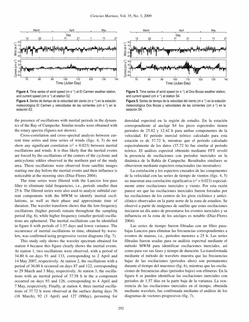
duration. The wavelet transform shows that the low-frequency

oscillations (higher period) remain throughout the sampling

period (fig. 6), while higher frequency (smaller period) oscilla-

tions are ephemeral. The inertial oscillations can be identified

in figure 6 with periods of 1.57 days and lower variance. The

occurrence of inertial oscillations in time, obtained by wave-

lets, was confirmed using progressive vector diagrams (fig. 7).

This study only shows the wavelet spectrum obtained for

station 4 because this figure clearly shows the inertial events.

At station 1, two oscillations were observed, with a period of

34.80 h on days 91 and 133, corresponding to 2 April and

14 May 2007, respectively. At station 2, the oscillations with a

period of 36.00 h occurred on days 87 and 122, corresponding

to 29 March and 3 May, respectively. At station 3, the oscilla-

tions with an inertial period of 37.58 h in the u component

occurred on days 93 and 126, corresponding to 4 April and

7 May, respectively. Finally, at station 4, three inertial oscilla-

tions of 37.72 h were observed at the surface during days 76

(18 March), 92 (3 April) and 127 (8May), persisting for

densidad espectral en la región de estudio. En la estación

correspondiente al anclaje S4 los picos espectrales tienen

periodos de 25.82 y 12.42 h para ambas componentes de la

velocidad. El periodo inercial teórico calculado para esta

estación es de 37.72 h, mientras que el periodo calculado

espectralmente de los datos (37.72 h) fue similar al periodo

teórico. El análisis espectral obtenido mediante FFT reveló

la presencia de oscilaciones con periodos inerciales en la

dinámica de la Bahía de Campeche. Resultados similares se

obtuvieron mediante espectros rotacionales (no mostrados).

La correlación y los espectros cruzados de las componentes

de la velocidad con las series de tiempo de vientos (figs. 4, 5)

no muestran una correlación significativa (r2 = 0.023) especial-

mente entre oscilaciones inerciales y viento. Por esta razón

parece ser que las oscilaciones inerciales fueron forzadas por

las oscilaciones de los centros de los giros ciclónico y antici-

clónico observados en la parte norte de la zona de estudios. Se

observó a partir de imágenes de satélite que estas oscilaciones

iniciaron un día antes de presentarse los eventos inerciales y su

influencia en la zona de los anclajes es notable (Díaz-Flores

2004).

Las series de tiempo fueron filtradas con un filtro pasa-

bajas Lanczos para eliminar las frecuencias correspondientes a

eventos de mareas, i.e., periodos menores a 25 h. Las series

filtradas fueron usadas para su análisis espectral mediante el

método MWM para identificar oscilaciones inerciales, así

como para ver sus fases y tiempo de duración. La transformada

mediante el método de wavelets muestra que las frecuencias

bajas de las oscilaciones (periodos altos) son permanentes

durante el tiempo del muestreo (fig. 6), mientras que las oscila-

ciones de frecuencias altas (periodos bajos) son efímeras. En la

figura 6 se pueden identificar las oscilaciones inerciales con

periodos de 1.57 días en la parte baja de la varianza. La ocu-

rrencia de las oscilaciones inerciales en el tiempo, obtenida

mediante wavelets, fue confirmada mediante el análisis de los

diagramas de vectores progresivos (fig. 7).

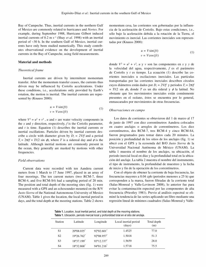
Figure 4. Time series of wind speed (m s–1) at El Carmen weather station,

and current speed (cm s–1) at station S2.

Figura 4. Series de tiempo de la velocidad del viento (m s–1) en la estación

meteorológica El Carmen y velocidades de las corrientes (cm s–1) en laestación S2.

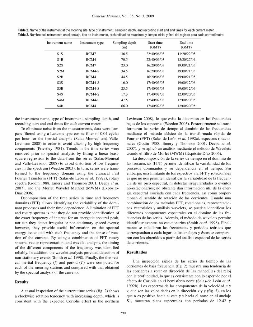
Figure 5. Time series of wind speed (m s–1) at Dos Bocas weather station,

and current speed (cm s–1) at station S4.

Figura 5. Series de tiempo de la velocidad del viento (m s–1) en la estación

meteorológica Dos Bocas y velocidades de las corrientes (cm s–1) en laestación S4.

-20

-10

0

10

20

0

20

40

20

-40

March

Day

MayApril

-20

-10

0

10

20

0

20

40

20

-40

March

Day

MayApril


293

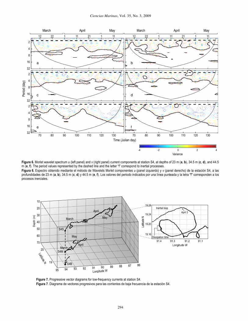
approximately 10 days. Figure 7 shows the progressive vector

diagrams at station 4 with the corresponding inertial loop on 3

April and the trajectory and dissipation time of the inertial

event.

Discussion

In the northernmost section (station 1) the amplitude of the

inertial oscillations was slightly higher for the v component

than for the u component, decaying slowly with depth. Diag-

nostic calculations (Xing and Davies 2004) show that, in the

near-coastal region, inertial oscillations are inhibited by the

coastal boundary. Away from the boundary, the magnitude of

the inertial oscillations increases, showing a 180º phase shift in

the vertical. This feature was observed at stations 2 and 4,

where the amplitude of the inertial oscillations was slightly

higher below the upper layer. The wavelet method revealed

inertial oscillations of two and three days duration. The pro-

gressive vector diagram shows that the dissipation time of the

inertial events is between 6 and 9 h. This is consistent with

Pollard (1970) and Millard (1970), who also found that the

evolution and decline of the inertial currents are due to a dis-

persion of the inertial oscillations generated within the region.

The disappearance of the inertial oscillations is usually pro-

duced by a second wind pulse with opposite direction to the

one that forced the inertial oscillations in the surface layer.

Smith (1973) supported this argument. Kundu (1976) stated

that this is possible, but suggested that it is not the only factor

responsible for the intermittence of the inertial oscillations.

Intermittence is produced by several mechanisms, such as the

horizontal heterogeneity of the ocean, the horizontal compo-

nent of the Coriolis parameter, and non-linear interactions with

currents of low frequencies (Hasselman 1970), as in this study.

The amplitude of tidal currents found in this study is small

when compared with total motion amplitudes. During the

sampling period, several episodes of inertial currents were

observed, some of which corresponded to those predicted by

theory. The currents in the lower layer are not strongly linked

to those at the surface. A typical phase lag of 0.85 h for M2 and

3.46 h for K1 is observed between lower and upper layers, evi-

dencing that the inertial currents have a baroclinic first mode.

The spectral energy was concentrated at the low-frequency

bands, corresponding to tidal and inertial periods. Some of

these oscillations were also observed in the progressive vector

diagrams in a semicircular path. The dominance of the MWM

spectral energy at low frequencies revealed the influence of the

mesoscale cyclonic and small anticyclonic eddies of the north-

eastern Bay of Campeche. This was because the oscillations of

the cyclonic and anticyclonic eddy cores observed in the north-

eastern part of the study area were highly correlated with the

inertial events. Those eddies can be the origin for the inertial

currents because the observed inertial currents were unrelated

to wind forcing. Similar responses have been reported for other

regions of the world ocean (Benitez-Nelson and McGillicuddy

2008).

En este estudio se muestra sólo el resultado del espectro

obtenido mediante el método de wavelets Morlet de la estación

S4, ya que esta figura es la que muestra más claramente

los eventos inerciales. En la estación S1 se observaron dos

oscilaciones con periodos de 34.80 h durante los días 91 y

133, correspondientes al 2 de abril y 14 de mayo de 2007,

respectivamente. En la estación S2 se encontraron oscilaciones

inerciales con periodos de 36.00 h durante los días 87 y 122,

que corresponden al 29 de marzo y al 3 de mayo, respectiva-

mente. En la estación S3, las oscilaciones observadas con un

periodo inercial de 37.58 h en la componente u ocurrieron

durante los días 93 y 126, que corresponden al 4 de abril y 7 de

mayo, respectivamente. Finalmente, en la estación S4 se

observaron tres oscilaciones inerciales con periodos de 37.72 h

en la serie de datos del correntímetro superficial durante los

días 76 (18 de marzo), 92 (3 de abril) y 127 (8 de mayo),

persistiendo por aproximadamente 10 días. La figura 7 muestra

el diagrama de vectores progresivos para la estación S4 con un

rizo inercial durante el 3 de abril, así como su trayectoria y

tiempo de disipación.

Discusión

En la porción más al norte (estación 1) la amplitud de las

oscilaciones inerciales fue ligeramente mayor para la compo-

nente v que para la componente u de las corrientes y decayó

suavemente con la profundidad, mientras que en las otras tres

localidades u es más grande que la componente v. Cálculos

efectuados por Xing y Davis (2004) muestran que, cerca de la

costa, las oscilaciones inerciales son inhibidas por la frontera,

que es la costa. Al alejarse de la costa la magnitud de las osci-

laciones inerciales se incrementa, mostrando un defasamiento

de 180° en la vertical. Esta característica se observó en las esta-

ciones 2 y 4, donde la amplitud de las oscilaciones inerciales

fue ligeramente mayor debajo de la capa superficial. El método

de wavelets reveló la ocurrencia de oscilaciones inerciales con

duraciones de dos y tres días. El diagrama de vectores progre-

sivos muestra que el tiempo de disipación de los eventos iner-

ciales fue entre 6 y 9 h. Esto es consistente con lo encontrado

por Pollard (1970) y Millard (1970), quienes también encontra-

ron que la evolución y declive de las corrientes inerciales se

deben a la dispersión de las oscilaciones inerciales generada en

la región. La desaparición de las oscilaciones inerciales es

usualmente producida por un segundo impulso de viento en

dirección opuesta a la del forzamiento que produjo la oscila-

ción inercial en la capa superficial. Smith (1973) apoya este

argumento. Kundo (1976) dice que es posible, sin embargo

sugiere que éste no es el único factor responsable de la intermi-

tencia de las oscilaciones inerciales. La intermitencia se pro-

duce por varios mecanismos tales como la heterogeneidad en

las condiciones horizontales del océano, la componente hori-

zontal del parámetro de Coriolis y la no linealidad de las inte-

racciones de las corrientes de baja frecuencia (Hasselman

1970), como es el caso en este estudio.


294

Figure 6. Morlet wavelet spectrum u (left panel) and v (right panel) current components at station S4, at depths of 23 m (a, b), 34.5 m (c, d), and 44.5m (e, f). The period values represented by the dashed line and the letter “f” correspond to inertial processes.

Figura 6. Espectro obtenido mediante el método de Wavelets Morlet componentes u (panel izquierdo) y v (panel derecho) de la estación S4, a lasprofundidades de 23 m (a, b), 34.5 m (c, d) y 44.5 m (e, f). Los valores del periodo indicados por una línea punteada y la letra "f" corresponden a losprocesos inerciales.

0 2 4

70 80 90 100 110 120 130 70 80 90 100 110 120 130

Variance

2

4

8

16

32

2

4

8

16

32

2

4

8

16

32

Period (day)

12 22 1 11 21 1 11 12 22 1 11 21 1 11

March April May March April May

-4 -2

Time (Julian day)

a b

d

f

c

e

95 94 93 92 91 90 89 88 87 8619

20

70

60

50

40

30

20

10

Longitude W

Latitude N

Dep

th (

m)

S4B

S4M

S4S

May

MarchApril

May

April

March

19.16

19.20

19.24

19.28

April 3

Dissipation time

Inertial loop

Figure 7. Progressive vector diagrams for low-frequency currents at station S4.

Figura 7. Diagrama de vectores progresivos para las corrientes de baja frecuencia de la estación S4.


295

This study describes the presence of a low-frequency com-

ponent in current velocities in the southern Gulf of Mexico.

The low frequency variations are related to inertial oscillations

with an approximate duration of three days. Spectral analysis

indicated that inertial and semidiurnal frequency motions were

the major contributors to current velocities. The observed near-

inertial frequency was about 0.1% lower than the local inertial

frequency, suggesting that the near-inertial motion was embed-

ded in a region of anticyclonic shear.

The highest spectral energy in the inertial oscillations cor-

responded to the north-south current component, which

decayed slowly with depth, although in some cases, as at sta-

tions 2 and 4, the spectral density was slightly higher near the

bottom than in the surface layer. In turn, in the east-west com-

ponent, the current amplitude increased seaward reaching a

maximum near the shelf break. During the three months of

observations, several episodes of inertial currents were

observed. The frequencies of these events obtained from the

data coincided with those predicted by theory.

Acknowledgements

This study was financed by PEMEX and the Institute

of Marine Science and Limnology (UNAM). We would like

to acknowledge the crew and officers of the R/V Justo Sierra

for their dedication during the different stages of sampling.

Figures were substantially inproved by J Castro.

References

Behringer DW, Molinari RL, Festas JF. 1977. The variability of

anticyclonic current patterns in the Gulf of Mexico. J. Geophys.Res. 82: 5469–5476.

Benitez-Nelson CR, McGillicuddy Jr. DJ. 2008. Mesoscale physical-

biological-biogeochemical linkages in the open ocean: An

introduction to the results of the E-Flux and EDDIES programs.Deep-Sea Res. II 55: 1133–1138.

Cochrane JD. 1972. Separation of an anticyclone and subsequent

developments in the Loop Current (1969). In: Capurro LRA, ReidJL (eds.), Contributions on the Physical Oceanography of the Gulf

of Mexico. Gulf Publishing Co., Houston, Texas, pp. 91–106.

Deepa R, Seetaramayya P, Nagar SG, Gnanaseelan C. 2007. Inertial

oscillation forced by the September 1997 cyclone in the Bay ofBengal. Curr. Sci. 92: 790–794.

Díaz-Flores MA. 2004 Estudios de las corrientes en la Bahía de

Campeche utulizando un perfilador acústico Doppler (ADCP).M.Sc. thesis, Universidad Nacional Autónoma de México, 67 pp.

Emery WJ, Thomson RE. 2001. Data Analysis Methods in Physical

Oceanography. 2nd and revised ed. Elsevier, Amsterdam, 654 pp.

Expósito-Díaz G. 2006. Corrientes inerciales al sur del Golfo deMéxico. M.Sc. thesis, Universidad Nacional Autónoma de

México, 94 pp.

Godin G. 1988. Tides. Centro de Investigación Científica y de

Educación Superior de Ensenada (CICESE), Ensenada, Mexico,290 pp.

Hasselman K. 1970. Wave-driven inertial oscillations. Geophys.

Astrophys. Fluid Dyn. 1: 463–502.

Hernández-Téllez J, Aldeco J, Salas-de León DA. 1993. Cooling andheating due to latent and sensible heat over the Yucatan

continental shelf. Atmósfera 6: 223–233.

La amplitud de las corrientes de marea encontradas en este

trabajo fue pequeña comparada con las amplitudes de las

corrientes totales. Durante el tiempo del muestreo se observa-

ron varios episodios de corrientes inerciales, algunos de los

cuales correspondieron en periodo con los predichos por la teo-

ría. Las corrientes en las capas profundas no estuvieron fuerte-

mente ligadas con las de la superficie. Se observó un

defasamiento típico de 0.85 h para la M2 y de 3.46 h para la K1

entre las capas superficiales y las profundas, lo que evidencia

que las corrientes inerciales corresponden a un primer modo

baroclínico. La energía espectral se concentró en la banda de

las frecuencias bajas, correspondiendo a periodos de marea e

inerciales. Algunas de estas oscilaciones fueron observadas

también en el diagrama de vectores progresivos mediante

trayectorias semicirculares. La energía dominante en el

espectro obtenido por el método de wavelets con Morlet reveló

la influencia de los giros ciclónicos y anticiclónicos de

mesoescala del norte de la Bahía de Campeche. Esto se debe a

que las oscilaciones del centro de los giros ciclónicos y

anticiclónicos observadas en la parte norte de la zona de

estudio estuvieron fuertemente correlacionadas con los eventos

inerciales. Las oscilaciones de los centros de estos giros

pueden ser las que forzaron las corrientes inerciales, ya que

estas corrientes no mostraron una correlación significativa con

el forzamiento por viento. En otras regiones de los océanos en

el mundo se han reportado respuestas similares (Benitez-

Nelson y McGillicuddy 2008).

Este estudio describe la presencia de componentes de baja

frecuencia en las velocidades de las corrientes en el sur del

Golfo de México. Las variaciones en las frecuencias bajas

están relacionadas con las oscilaciones inerciales con duración

aproximada de tres días. El análisis espectral indica que los

movimientos con frecuencias inerciales y los semidiurnos son

las componentes más importantes de las corrientes. Las

diferencias entre las frecuencias inerciales observadas y las

teóricas fue menor a 0.1%. Estos resultados sugieren que los

movimientos inerciales estuvieron insertados en una región de

esfuerzos tangenciales de un giro anticiclónico.

La mayor energía espectral de las oscilaciones inerciales

correspondió a la componente norte-sur de las corrientes, la

cual decayó suavemente con la profundidad; sin embargo, en

algunos casos como en las estaciones 2 y 4, la densidad espec-

tral fue ligeramente mayor cerca del fondo que en la capa

superficial. A su vez, la amplitud de la componente este-oeste

de las corrientes se incrementó mar adentro alcanzando un

máximo cerca del borde del talud. Durante los tres meses de

observaciones se detectaron varios episodios de corrientes

inerciales. Las frecuencias de estos eventos coincidieron con

los predichos por la teoría.

Agradecimientos

Este trabajo fue financiado por PEMEX y por el Instituto

de Ciencias del Mar y Limnología de la Universidad Nacional

Autónoma de México (UNAM). Los autores agradecen a la


296

Knauss JA. 2000. Introduction to Physical Oceanography. Prentice

Hall, New Jersey, 309 pp.

Kundu PK. 1976. An analysis of inertial oscillations observed near

Oregon coast. J. Phys. Oceanogr. 6: 879–893.

Merrel WJ Jr, Morrison JM. 1981. On the circulation of the Gulf of

Mexico with observations from April 1978. J. Geophys. Res. 86:4181–4185.

Millard RC. 1970. Comparison between observed and simulated

wind-generated inertial oscillations. Deep-Sea Res. 17: 813–821.

Monreal-Gómez MA, Salas-de León DA. 1997. Circulación yestructura termohalina del Golfo de México. In: Lavín-Peregrina

MF (ed.), Oceanografía Física en México. Monografía No. 3 de la

Unión Geofísica Mexicana, pp. 183–199.

Nowlin WD Jr. 1972. Winter circulation patterns and property

distributions. In: Capurro LRA, Reid JL (eds.), Contributions on

the Physical Oceanography of the Gulf of Mexico. GulfPublishing Co., Houston, Texas, pp. 3–15.

Pickett RL, Partridge RM, Arnone RA, Galt JA. 1984. The Persian

Gulf, oil and natural circulation. Sea Tech. 9: 23–25.

Pingree RD, Mardell GT, Holligan PM, Griffiths DK, Smithers J.1982. Celtic Sea and Armorican Current structure and the vertical

distributions of temperature and chlorophyll. Cont. Shelf Res. 1:

99–116.

Pollard RT. 1970. On the generation by winds of inertial oscillationsin the ocean. Deep-Sea Res. 17: 795–812.

Priestley MB. 1981. Spectral Analysis and Time Series. Academic

Press, London, 237 pp.

Salas-de León DA, Monreal-Gómez MA. 1986. The role of the LoopCurrent in the Gulf of Mexico fronts. In: Nihoul JCJ (ed.), Marine

Interfaces Ecohydrodynamics. Elsevier Oceanographic Series,

pp. 295–300.

Salas-de León DA, Monreal-Gómez MA, Aldeco-Ramírez J. 1992a.

Períodos característicos en las oscilaciones de parámetros

meteorológicos en Cayo Arcas, México. Atmósfera 5: 193–205.

Salas-de León DA, Monreal-Gómez MA, Colunga-Enríquez G.1992b. Hidrografía y circulación geostrófica en el sur de la Bahía

de Campeche. Geofís. Int. 3: 315–323.

tripulación y oficiales del B/O Justo Sierra por su dedicación

durante las diferentes etapas del muestreo. Las figuras fueron

mejoradas sustancialmente por J Castro.

Salas-de León DA, Monreal-Gómez MA, Salas-Monreal D, Expósito-

Díaz G, Riverón-Enzástiga ML, Vázquez-Gutiérrez F. 2007. Tidal

current components in the southern Bay of Campeche, Gulf ofMexico. Geofís. Int. 2: 141–147.

Salas-Monreal D, Valle-Levinson A. 2008. Sea level slopes and

volume fluxes produced by atmospheric forcing in estuaries:

Chesapeake Bay by case. J. Coast. Res. 6: 1–10.

Schumann EH, Churchill JRS, Zaayman HJ. 2005. Oceanic variability

in the western sector of Algoa Bay, South Africa. Afr. J. Mar. Sci.

1: 65–80.

Shay LK, Mariano AJ, Jacob SD, Ryan EH. 1998. Mean and near-inertial ocean current response to Hurricane Gilbert. J. Phys.

Oceanogr. 5: 858–889.

Smith LC, Turcotte D, Isacks BL. 1998. Stream flow characterizationand feature detection using a discrete wavelet transform. Hydrol.

Process. 12: 233–249.

Smith R. 1973. Evolution of inertial frequency oscillations. J. Fluid

Mech. 60: 383–389.

Van Haren H, Maas L, Zimmerman JTF, Ridderinkhof H, Malschaert

H. 1999. Strong inertial currents and marginal internal wave

stability in the central North Sea. J. Geophys. Res. L. 19:2993–2996.

Weedon G. 2003. Time-series Analysis and Cyclostratigraphy.

Examining Stratigraphic Records of Environmental Cycles.

Cambridge Univ. Press, 259 pp.

Xing J, Davies AM. 2004. A three-dimensional model study of near-

inertial motion: Generation and influence of an along-shelf flow.

Ocean Dyn. 2: 163–178.

Recibido en febrero de 2008;

aceptado en agosto de 2009.

inertial currents in the southern gulf of mexico ... · expósito-díaz et al.: inertial currents...

Documents