inexact newton methods and pde-constrained optimization
TRANSCRIPT

PDE Optimization Inexact Newton methods Experimental results Conclusion
Inexact Newton Methods andPDE-Constrained Optimization
Frank E. Curtis
COPTA Lecture SeriesUniversity of Wisconsin at Madison
April 24, 2009
Inexact Newton Methods and PDE-Constrained Optimization COPTA Lecture, U. Wisconsin

PDE Optimization Inexact Newton methods Experimental results Conclusion
Outline
PDE-Constrained Optimization
Inexact Newton methods
Experimental results
Conclusion and final remarks
Inexact Newton Methods and PDE-Constrained Optimization COPTA Lecture, U. Wisconsin

PDE Optimization Inexact Newton methods Experimental results Conclusion
Outline
PDE-Constrained Optimization
Inexact Newton methods
Experimental results
Conclusion and final remarks
Inexact Newton Methods and PDE-Constrained Optimization COPTA Lecture, U. Wisconsin

PDE Optimization Inexact Newton methods Experimental results Conclusion
Hyperthermia treatment
I Regional hyperthermia is a cancer therapy that aims at heating large anddeeply seated tumors by means of radio wave adsorption
I Results in the killing of tumor cells and makes them more susceptible toother accompanying therapies; e.g., chemotherapy
Inexact Newton Methods and PDE-Constrained Optimization COPTA Lecture, U. Wisconsin

PDE Optimization Inexact Newton methods Experimental results Conclusion
Hyperthermia treatment planning
I Computer modeling can be used to help plan the therapy for eachpatient, and it opens the door for numerical optimization
I The goal is to heat the tumor to a target temperature of 43C whileminimizing damage to nearby cells
Inexact Newton Methods and PDE-Constrained Optimization COPTA Lecture, U. Wisconsin

PDE Optimization Inexact Newton methods Experimental results Conclusion
Hyperthermia treatment as an optimization problem
The problem is to
miny,u
∫Ω
(y − yt)2dV where yt =
37 in Ω\Ω0
43 in Ω0
subject to the bio-heat transfer equation (Pennes (1948))
− ∇ · (κ∇y)︸ ︷︷ ︸thermal conductivity
+ ω(y)π(y − yb)︸ ︷︷ ︸effects of blood flow
= σ2
∣∣∑i ui Ei
∣∣2︸ ︷︷ ︸electromagnetic field
, in Ω
and the bound constraints
y ≤ 37.5, on ∂Ω
y ≥ 41.0, in Ω0
where Ω0 is the tumor domain
Inexact Newton Methods and PDE-Constrained Optimization COPTA Lecture, U. Wisconsin

PDE Optimization Inexact Newton methods Experimental results Conclusion
ApplicationsModel calibration Data assimilation
Image registrationOptimal design/control
(Walker et al., 2009)
Inexact Newton Methods and PDE-Constrained Optimization COPTA Lecture, U. Wisconsin
PDE Optimization Inexact Newton methods Experimental results Conclusion
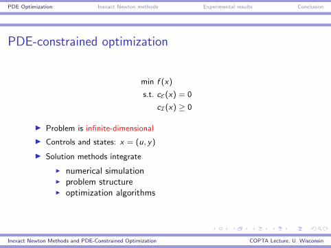
PDE-constrained optimization
min f (x)
s.t. cE(x) = 0
cI(x) ≥ 0
I Problem is infinite-dimensional
I Controls and states: x = (u, y)
I Solution methods integrate
I numerical simulationI problem structureI optimization algorithms
Inexact Newton Methods and PDE-Constrained Optimization COPTA Lecture, U. Wisconsin

PDE Optimization Inexact Newton methods Experimental results Conclusion
Algorithmic frameworks
We hear the phrases:
I Discretize-then-optimize
I Optimize-then-discretize
I prefer:
I Discretize the optimization problem
min f (x)
s.t. c(x) = 0⇒
min fh(x)
s.t. ch(x) = 0
I Discretize the optimality conditions
min f (x)
s.t. c(x) = 0⇒
[∇f + 〈A, λ〉
c
]= 0 ⇒
[(∇f + 〈A, λ〉)h
ch
]= 0
I Discretize the search direction computation
Inexact Newton Methods and PDE-Constrained Optimization COPTA Lecture, U. Wisconsin

PDE Optimization Inexact Newton methods Experimental results Conclusion
Algorithms
I Nonlinear elimination
minu,y
f (u, y)
s.t. c(u, y) = 0⇒ min
uf (u, y(u)) ⇒ ∇uf +∇uyT∇y f = 0
I Reduced-space methods
dy : toward satisfying the constraints
λ : Lagrange multiplier estimates
du : toward optimality
I Full-space methodsHu 0 ATu
0 Hy ATy
Au Ay 0
du
dy
δ
= −
∇uf + ATu λ
∇y f + ATy λ
c
Inexact Newton Methods and PDE-Constrained Optimization COPTA Lecture, U. Wisconsin
PDE Optimization Inexact Newton methods Experimental results Conclusion
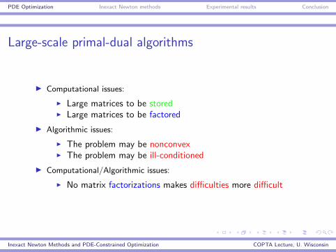
Large-scale primal-dual algorithms
I Computational issues:
I Large matrices to be storedI Large matrices to be factored
I Algorithmic issues:
I The problem may be nonconvexI The problem may be ill-conditioned
I Computational/Algorithmic issues:
I No matrix factorizations makes difficulties more difficult
Inexact Newton Methods and PDE-Constrained Optimization COPTA Lecture, U. Wisconsin

PDE Optimization Inexact Newton methods Experimental results Conclusion
Outline
PDE-Constrained Optimization
Inexact Newton methods
Experimental results
Conclusion and final remarks
Inexact Newton Methods and PDE-Constrained Optimization COPTA Lecture, U. Wisconsin
PDE Optimization Inexact Newton methods Experimental results Conclusion
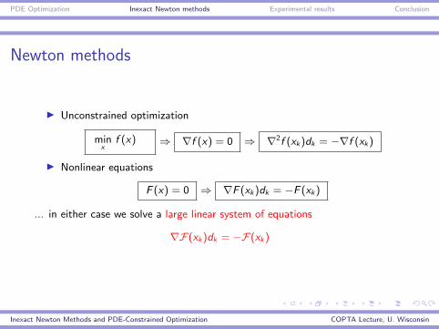
Newton methods
I Unconstrained optimization
minx
f (x) ⇒ ∇f (x) = 0 ⇒ ∇2f (xk)dk = −∇f (xk)
I Nonlinear equations
F (x) = 0 ⇒ ∇F (xk)dk = −F (xk)
... in either case we solve a large linear system of equations
∇F(xk)dk = −F(xk)
Inexact Newton Methods and PDE-Constrained Optimization COPTA Lecture, U. Wisconsin
PDE Optimization Inexact Newton methods Experimental results Conclusion
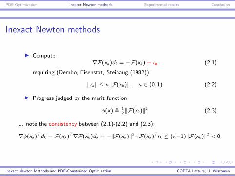
Inexact Newton methods
I Compute∇F(xk)dk = −F(xk) + rk (2.1)
requiring (Dembo, Eisenstat, Steihaug (1982))
‖rk‖ ≤ κ‖F(xk)‖, κ ∈ (0, 1) (2.2)
I Progress judged by the merit function
φ(x) , 12‖F(xk)‖2 (2.3)
... note the consistency between (2.1)-(2.2) and (2.3):
∇φ(xk)T dk = F(xk)T∇F(xk)dk = −‖F(xk)‖2+F(xk)T rk ≤ (κ−1)‖F(xk)‖2 < 0
Inexact Newton Methods and PDE-Constrained Optimization COPTA Lecture, U. Wisconsin

PDE Optimization Inexact Newton methods Experimental results Conclusion
Equality constrained optimization
I Considerminx∈Rn
f (x)
s.t. c(x) = 0
I Lagrangian isL(x , λ) , f (x) + λT c(x)
so the first-order optimality conditions are
∇L(x , λ) =
[∇f (x) +∇c(x)λ
c(x)
], F(x , λ) = 0
Inexact Newton Methods and PDE-Constrained Optimization COPTA Lecture, U. Wisconsin

PDE Optimization Inexact Newton methods Experimental results Conclusion
Newton methods and sequential quadratic programmingIf H(xk , λk) is positive definite on the null space of ∇c(xk)T , then[
H(xk , λk) ∇c(xk)∇c(xk)T 0
] [dδ
]= −
[∇f (xk) +∇c(xk)λk
c(xk)
]is equivalent to
mind∈Rn
f (xk) +∇f (xk)T d + 12dT H(xk , λk)d
s.t. c(xk) +∇c(xk)T d = 0
Inexact Newton Methods and PDE-Constrained Optimization COPTA Lecture, U. Wisconsin
PDE Optimization Inexact Newton methods Experimental results Conclusion
Merit function
I Simply minimizing
ϕ(x , λ) = 12‖F(x , λ)‖2 = 1
2
∥∥∥∥[∇f (x) +∇c(x)λc(x)
]∥∥∥∥2
is generally inappropriate for constrained optimization
I We use the merit function
φ(x ;π) , f (x) + π‖c(x)‖
where π is a penalty parameter
Inexact Newton Methods and PDE-Constrained Optimization COPTA Lecture, U. Wisconsin
PDE Optimization Inexact Newton methods Experimental results Conclusion
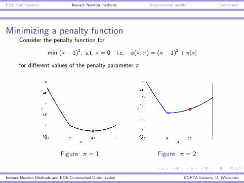
Minimizing a penalty functionConsider the penalty function for
min (x − 1)2, s.t. x = 0 i.e. φ(x ;π) = (x − 1)2 + π|x |
for different values of the penalty parameter π
Figure: π = 1 Figure: π = 2
Inexact Newton Methods and PDE-Constrained Optimization COPTA Lecture, U. Wisconsin

PDE Optimization Inexact Newton methods Experimental results Conclusion
Algorithm 0: Newton method for optimization
(Assume the problem is convex and regular)for k = 0, 1, 2, . . .
I Solve the primal-dual (Newton) equations[H(xk , λk) ∇c(xk)∇c(xk)T 0
] [dk
δk
]= −
[∇f (xk) +∇c(xk)λk
c(xk)
]I Increase π, if necessary, so that πk ≥ ‖λk + δk‖ (yields Dφk(dk ;πk) 0)
I Backtrack from αk ← 1 to satisfy the Armijo condition
φ(xk + αkdk ;πk) ≤ φ(xk ;πk) + ηαkDφk(dk ;πk)
I Update iterate (xk+1, λk+1)← (xk , λk) + αk(dk , δk)
Inexact Newton Methods and PDE-Constrained Optimization COPTA Lecture, U. Wisconsin

PDE Optimization Inexact Newton methods Experimental results Conclusion
Convergence of Algorithm 0
AssumptionThe sequence (xk , λk) is contained in a convex set Ω over which f , c, andtheir first derivatives are bounded and Lipschitz continuous. Also,
I (Regularity) ∇c(xk)T has full row rank with singular values boundedbelow by a positive constant
I (Convexity) uT H(xk , λk)u ≥ µ‖u‖2 for µ > 0 for all u ∈ Rn satisfyingu 6= 0 and ∇c(xk)T u = 0
Theorem(Han (1977)) The sequence (xk , λk) yields the limit
limk→∞
∥∥∥∥[∇f (xk) +∇c(xk)λk
c(xk)
]∥∥∥∥ = 0
Inexact Newton Methods and PDE-Constrained Optimization COPTA Lecture, U. Wisconsin

PDE Optimization Inexact Newton methods Experimental results Conclusion
Incorporating inexactness
I Iterative as opposed to direct methods
I Compute[H(xk , λk) ∇c(xk)∇c(xk)T 0
] [dk
δk
]= −
[∇f (xk) +∇c(xk)λk
c(xk)
]+
[ρk
rk
]satisfying ∥∥∥∥[ρk
rk
]∥∥∥∥ ≤ κ ∥∥∥∥[∇f (xk) +∇c(xk)λk
c(xk)
]∥∥∥∥ , κ ∈ (0, 1)
I If κ is not sufficiently small (e.g., 10−3 vs. 10−12), then dk may be anascent direction for our merit function; i.e.,
Dφk(dk ;πk) > 0 for all πk ≥ πk−1
Inexact Newton Methods and PDE-Constrained Optimization COPTA Lecture, U. Wisconsin
PDE Optimization Inexact Newton methods Experimental results Conclusion
Model reductions
I Define the model of φ(x ;π):
m(d ;π) , f (x) +∇f (x)T d + π(‖c(x) +∇c(x)T d‖)
I dk is acceptable if
∆m(dk ;πk) , m(0;πk)−m(dk ;πk)
= −∇f (xk)T dk + πk(‖c(xk)‖ − ‖c(xk) +∇c(xk)T dk‖) 0
I This ensures Dφk(dk ;πk) 0 (and more)
Inexact Newton Methods and PDE-Constrained Optimization COPTA Lecture, U. Wisconsin
PDE Optimization Inexact Newton methods Experimental results Conclusion
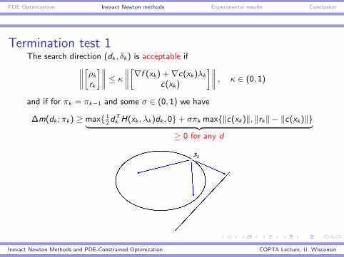
Termination test 1The search direction (dk , δk) is acceptable if∥∥∥∥[ρk
rk
]∥∥∥∥ ≤ κ ∥∥∥∥[∇f (xk) +∇c(xk)λk
c(xk)
]∥∥∥∥ , κ ∈ (0, 1)
and if for πk = πk−1 and some σ ∈ (0, 1) we have
∆m(dk ;πk) ≥ max 12dT
k H(xk , λk)dk , 0+ σπk max‖c(xk)‖, ‖rk‖ − ‖c(xk)‖︸ ︷︷ ︸≥ 0 for any d
Inexact Newton Methods and PDE-Constrained Optimization COPTA Lecture, U. Wisconsin
PDE Optimization Inexact Newton methods Experimental results Conclusion
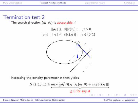
Termination test 2The search direction (dk , δk) is acceptable if
‖ρk‖ ≤ β‖c(xk)‖, β > 0
and ‖rk‖ ≤ ε‖c(xk)‖, ε ∈ (0, 1)
Increasing the penalty parameter π then yields
∆m(dk ;πk) ≥ max 12dT
k H(xk , λk)dk , 0+ σπk‖c(xk)‖︸ ︷︷ ︸≥ 0 for any d
Inexact Newton Methods and PDE-Constrained Optimization COPTA Lecture, U. Wisconsin
PDE Optimization Inexact Newton methods Experimental results Conclusion
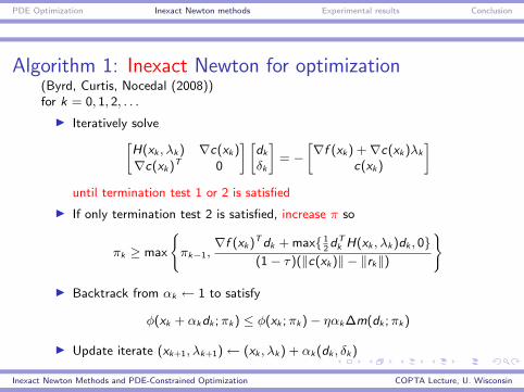
Algorithm 1: Inexact Newton for optimization(Byrd, Curtis, Nocedal (2008))for k = 0, 1, 2, . . .
I Iteratively solve[H(xk , λk) ∇c(xk)∇c(xk)T 0
] [dk
δk
]= −
[∇f (xk) +∇c(xk)λk
c(xk)
]until termination test 1 or 2 is satisfied
I If only termination test 2 is satisfied, increase π so
πk ≥ max
πk−1,
∇f (xk)T dk + max 12dT
k H(xk , λk)dk , 0(1− τ)(‖c(xk)‖ − ‖rk‖)
I Backtrack from αk ← 1 to satisfy
φ(xk + αkdk ;πk) ≤ φ(xk ;πk)− ηαk∆m(dk ;πk)
I Update iterate (xk+1, λk+1)← (xk , λk) + αk(dk , δk)
Inexact Newton Methods and PDE-Constrained Optimization COPTA Lecture, U. Wisconsin
PDE Optimization Inexact Newton methods Experimental results Conclusion
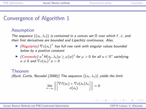
Convergence of Algorithm 1
AssumptionThe sequence (xk , λk) is contained in a convex set Ω over which f , c, andtheir first derivatives are bounded and Lipschitz continuous. Also,
I (Regularity) ∇c(xk)T has full row rank with singular values boundedbelow by a positive constant
I (Convexity) uT H(xk , λk)u ≥ µ‖u‖2 for µ > 0 for all u ∈ Rn satisfyingu 6= 0 and ∇c(xk)T u = 0
Theorem(Byrd, Curtis, Nocedal (2008)) The sequence (xk , λk) yields the limit
limk→∞
∥∥∥∥[∇f (xk) +∇c(xk)λk
c(xk)
]∥∥∥∥ = 0
Inexact Newton Methods and PDE-Constrained Optimization COPTA Lecture, U. Wisconsin
PDE Optimization Inexact Newton methods Experimental results Conclusion
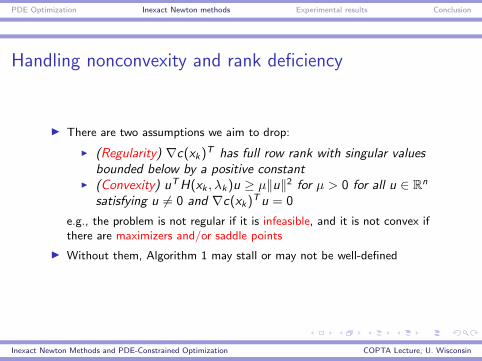
Handling nonconvexity and rank deficiency
I There are two assumptions we aim to drop:
I (Regularity) ∇c(xk)T has full row rank with singular valuesbounded below by a positive constant
I (Convexity) uTH(xk , λk)u ≥ µ‖u‖2 for µ > 0 for all u ∈ Rn
satisfying u 6= 0 and ∇c(xk)Tu = 0
e.g., the problem is not regular if it is infeasible, and it is not convex ifthere are maximizers and/or saddle points
I Without them, Algorithm 1 may stall or may not be well-defined
Inexact Newton Methods and PDE-Constrained Optimization COPTA Lecture, U. Wisconsin

PDE Optimization Inexact Newton methods Experimental results Conclusion
No factorizations means no clue
I We might not store or factor[H(xk , λk) ∇c(xk)∇c(xk)T 0
]so we might not know if the problem is nonconvex or ill-conditioned
I Common practice is to perturb the matrix to be[H(xk , λk) + ξ1I ∇c(xk)∇c(xk)T −ξ2I
]where ξ1 convexifies the model and ξ2 regularizes the constraints
I Poor choices of ξ1 and ξ2 can have terrible consequences in the algorithm
Inexact Newton Methods and PDE-Constrained Optimization COPTA Lecture, U. Wisconsin
PDE Optimization Inexact Newton methods Experimental results Conclusion
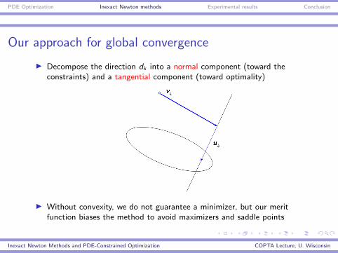
Our approach for global convergence
I Decompose the direction dk into a normal component (toward theconstraints) and a tangential component (toward optimality)
I Without convexity, we do not guarantee a minimizer, but our meritfunction biases the method to avoid maximizers and saddle points
Inexact Newton Methods and PDE-Constrained Optimization COPTA Lecture, U. Wisconsin
PDE Optimization Inexact Newton methods Experimental results Conclusion
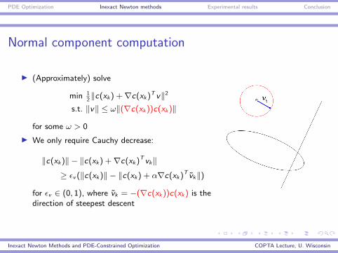
Normal component computation
I (Approximately) solve
min 12‖c(xk) +∇c(xk)T v‖2
s.t. ‖v‖ ≤ ω‖(∇c(xk))c(xk)‖
for some ω > 0
I We only require Cauchy decrease:
‖c(xk)‖ − ‖c(xk) +∇c(xk)T vk‖
≥ εv (‖c(xk)‖ − ‖c(xk) + α∇c(xk)T vk‖)
for εv ∈ (0, 1), where vk = −(∇c(xk))c(xk) is thedirection of steepest descent
Inexact Newton Methods and PDE-Constrained Optimization COPTA Lecture, U. Wisconsin

PDE Optimization Inexact Newton methods Experimental results Conclusion
Tangential component computation (idea #1)
I Standard practice is to then (approximately) solve
min (∇f (xk) + H(xk , λk)vk)T u + 12uT H(xk , λk)u
s.t. ∇c(xk)T u = 0, ‖u‖ ≤ ∆k
I However, maintaining
∇c(xk)T u ≈ 0 and ‖u‖ ≤ ∆k
can be expensive
Inexact Newton Methods and PDE-Constrained Optimization COPTA Lecture, U. Wisconsin

PDE Optimization Inexact Newton methods Experimental results Conclusion
Tangential component computation
I Instead, we formulate the primal-dual system[H(xk , λk) ∇c(xk)∇c(xk)T 0
] [uk
δk
]= −
[∇f (xk) +∇c(xk)λk + H(xk , λk)vk
0
]I Our ideas from before apply!
Inexact Newton Methods and PDE-Constrained Optimization COPTA Lecture, U. Wisconsin
PDE Optimization Inexact Newton methods Experimental results Conclusion
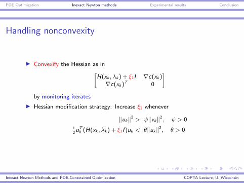
Handling nonconvexity
I Convexify the Hessian as in[H(xk , λk) + ξ1I ∇c(xk)∇c(xk)T 0
]by monitoring iterates
I Hessian modification strategy: Increase ξ1 whenever
‖uk‖2 > ψ‖vk‖2, ψ > 0
12uT
k (H(xk , λk) + ξ1I )uk < θ‖uk‖2, θ > 0
Inexact Newton Methods and PDE-Constrained Optimization COPTA Lecture, U. Wisconsin
PDE Optimization Inexact Newton methods Experimental results Conclusion
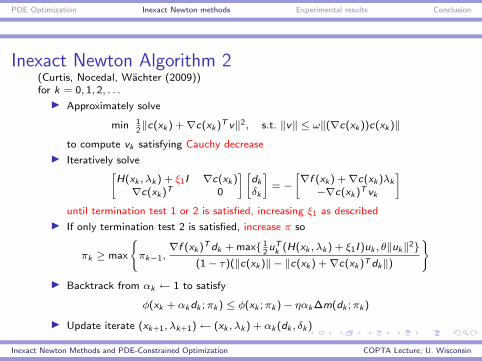
Inexact Newton Algorithm 2(Curtis, Nocedal, Wachter (2009))for k = 0, 1, 2, . . .
I Approximately solve
min 12‖c(xk ) +∇c(xk )T v‖2, s.t. ‖v‖ ≤ ω‖(∇c(xk ))c(xk )‖
to compute vk satisfying Cauchy decrease
I Iteratively solve[H(xk , λk ) + ξ1I ∇c(xk )∇c(xk )T 0
] [dk
δk
]= −
[∇f (xk ) +∇c(xk )λk
−∇c(xk )T vk
]until termination test 1 or 2 is satisfied, increasing ξ1 as described
I If only termination test 2 is satisfied, increase π so
πk ≥ max
πk−1,
∇f (xk )T dk + max 12uT
k (H(xk , λk ) + ξ1I )uk , θ‖uk‖2(1− τ)(‖c(xk )‖ − ‖c(xk ) +∇c(xk )T dk‖)
I Backtrack from αk ← 1 to satisfy
φ(xk + αkdk ;πk ) ≤ φ(xk ;πk )− ηαk∆m(dk ;πk )
I Update iterate (xk+1, λk+1)← (xk , λk ) + αk (dk , δk )
Inexact Newton Methods and PDE-Constrained Optimization COPTA Lecture, U. Wisconsin

PDE Optimization Inexact Newton methods Experimental results Conclusion
Convergence of Algorithm 2
AssumptionThe sequence (xk , λk) is contained in a convex set Ω over which f , c, andtheir first derivatives are bounded and Lipschitz continuous
Theorem(Curtis, Nocedal, Wachter (2009)) If all limit points of ∇c(xk)T have fullrow rank, then the sequence (xk , λk) yields the limit
limk→∞
∥∥∥∥[∇f (xk) +∇c(xk)λk
c(xk)
]∥∥∥∥ = 0.
Otherwise,lim
k→∞‖(∇c(xk))c(xk)‖ = 0
and if πk is bounded, then
limk→∞
‖∇f (xk) +∇c(xk)λk‖ = 0
Inexact Newton Methods and PDE-Constrained Optimization COPTA Lecture, U. Wisconsin
PDE Optimization Inexact Newton methods Experimental results Conclusion
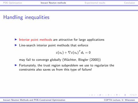
Handling inequalities
I Interior point methods are attractive for large applications
I Line-search interior point methods that enforce
c(xk) +∇c(xk)T dk = 0
may fail to converge globally (Wachter, Biegler (2000))
I Fortunately, the trust region subproblem we use to regularize theconstraints also saves us from this type of failure!
Inexact Newton Methods and PDE-Constrained Optimization COPTA Lecture, U. Wisconsin
PDE Optimization Inexact Newton methods Experimental results Conclusion
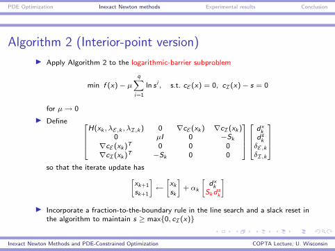
Algorithm 2 (Interior-point version)
I Apply Algorithm 2 to the logarithmic-barrier subproblem
min f (x)− µq∑
i=1
ln s i , s.t. cE(x) = 0, cI(x)− s = 0
for µ→ 0
I Define H(xk , λE,k , λI,k ) 0 ∇cE(xk ) ∇cI(xk )
0 µI 0 −Sk
∇cE(xk )T 0 0 0∇cI(xk )T −Sk 0 0
dxk
d sk
δE,kδI,k
so that the iterate update has[
xk+1
sk+1
]←[xk
sk
]+ αk
[dx
kSkd s
k
]I Incorporate a fraction-to-the-boundary rule in the line search and a slack reset in
the algorithm to maintain s ≥ max0, cI(x)
Inexact Newton Methods and PDE-Constrained Optimization COPTA Lecture, U. Wisconsin

PDE Optimization Inexact Newton methods Experimental results Conclusion
Convergence of Algorithm 2 (Interior-point)
AssumptionThe sequence (xk , λE,k , λI,k) is contained in a convex set Ω over which f ,cE , cI , and their first derivatives are bounded and Lipschitz continuous
Theorem(Curtis, Schenk, Wachter (2009))
I For a given µ, Algorithm 2 yields the same limits as in the equalityconstrained case
I If Algorithm 2 yields a sufficiently accurate solution to the barriersubproblem for each µj → 0 and if the linear independence constraintqualification (LICQ) holds at a limit point x of xj, then there existLagrange multipliers λ such that the first-order optimality conditions ofthe nonlinear program are satisfied
Inexact Newton Methods and PDE-Constrained Optimization COPTA Lecture, U. Wisconsin

PDE Optimization Inexact Newton methods Experimental results Conclusion
Outline
PDE-Constrained Optimization
Inexact Newton methods
Experimental results
Conclusion and final remarks
Inexact Newton Methods and PDE-Constrained Optimization COPTA Lecture, U. Wisconsin

PDE Optimization Inexact Newton methods Experimental results Conclusion
Implementation details
I Incorporated in IPOPT software package (Wachter)
I Linear systems solved with PARDISO (Schenk)
I Symmetric quasi-minimum residual method (Freund (1994))
I PDE-constrained model problems
I 3D grid Ω = [0, 1]× [0, 1]× [0, 1]I Equidistant Cartesian grid with N grid pointsI 7-point stencil for discretization
Inexact Newton Methods and PDE-Constrained Optimization COPTA Lecture, U. Wisconsin

PDE Optimization Inexact Newton methods Experimental results Conclusion
Boundary control problem
min 12
∫Ω(y(x)− yt(x))2dx , // yt(x) = 3 + 10x1(x1 − 1)x2(x2 − 1) sin(2πx3)
s.t. −∇ · (ey(x) · ∇y(x)) = 20, in Ω
y(x) = u(x), on ∂Ω, // u(x) defined on ∂Ω
2.5 ≤ u(x) ≤ 3.5, on ∂Ω
N n p q # nnz f ∗ # iter CPU sec20 8000 5832 4336 95561 1.3368e-2 12 33.430 27000 21952 10096 339871 1.3039e-2 12 139.440 64000 54872 18256 827181 1.2924e-2 12 406.050 125000 110592 28816 1641491 1.2871e-2 12 935.660 216000 195112 41776 2866801 1.2843e-2 13 1987.2
(direct) 40 64000 54872 18256 827181 1.2924e-2 10 3196.3
Inexact Newton Methods and PDE-Constrained Optimization COPTA Lecture, U. Wisconsin
PDE Optimization Inexact Newton methods Experimental results Conclusion
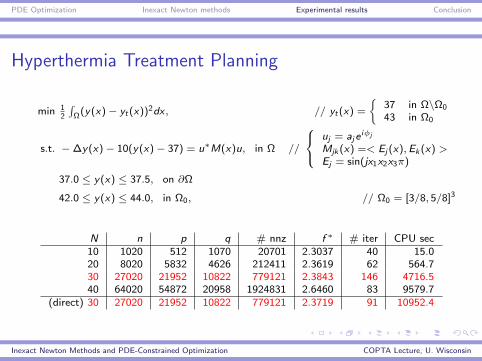
Hyperthermia Treatment Planning
min 12
∫Ω(y(x)− yt(x))2dx , // yt(x) =
37 in Ω\Ω0
43 in Ω0
s.t. −∆y(x)− 10(y(x)− 37) = u∗M(x)u, in Ω //
uj = ajeiφj
Mjk (x) =< Ej (x),Ek (x) >Ej = sin(jx1x2x3π)
37.0 ≤ y(x) ≤ 37.5, on ∂Ω
42.0 ≤ y(x) ≤ 44.0, in Ω0, // Ω0 = [3/8, 5/8]3
N n p q # nnz f ∗ # iter CPU sec10 1020 512 1070 20701 2.3037 40 15.020 8020 5832 4626 212411 2.3619 62 564.730 27020 21952 10822 779121 2.3843 146 4716.540 64020 54872 20958 1924831 2.6460 83 9579.7
(direct) 30 27020 21952 10822 779121 2.3719 91 10952.4
Inexact Newton Methods and PDE-Constrained Optimization COPTA Lecture, U. Wisconsin
PDE Optimization Inexact Newton methods Experimental results Conclusion
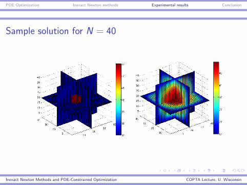
Sample solution for N = 40
Inexact Newton Methods and PDE-Constrained Optimization COPTA Lecture, U. Wisconsin

PDE Optimization Inexact Newton methods Experimental results Conclusion
Outline
PDE-Constrained Optimization
Inexact Newton methods
Experimental results
Conclusion and final remarks
Inexact Newton Methods and PDE-Constrained Optimization COPTA Lecture, U. Wisconsin

PDE Optimization Inexact Newton methods Experimental results Conclusion
Conclusion and final remarks
I PDE-Constrained optimization is an active and exciting area
I Inexact Newton method with theoretical foundation
I Convergence guarantees are as good as exact methods, sometimes better
I Numerical experiments are promising so far, and more to come
Inexact Newton Methods and PDE-Constrained Optimization COPTA Lecture, U. Wisconsin