inference for bivariate conway-maxwell-poisson
TRANSCRIPT

Inference for Bivariate Conway-Maxwell-Poisson
Distribution and Its Application in Modeling
Bivariate Count Data

INFERENCE FOR BIVARIATE CONWAY-MAXWELL-POISSON
DISTRIBUTION AND ITS APPLICATION IN MODELING
BIVARIATE COUNT DATA
BY
XINYI WANG, B.Sc.
a thesis
submitted to the department of mathematics & statistics
and the school of graduate studies
of mcmaster university
in partial fulfilment of the requirements
for the degree of
master of science
c© Copyright by Xinyi Wang, September 2019
All Rights Reserved

Master of Science (2019) McMaster University
(Mathematics & Statistics) Hamilton, Ontario, Canada
TITLE: Inference for Bivariate Conway-Maxwell-Poisson Distri-
bution and Its Application in Modeling Bivariate Count
Data
AUTHOR: Xinyi Wang
B.Sc., ( Actuarial and Financial Math )
McMaster University, Hamilton, Canada
SUPERVISOR: Dr. Narayanaswamy Balakrishnan
NUMBER OF PAGES: x, 59
ii

To my parents, Hong and Hao.

Abstract
In recent actuarial literature, the bivariate Poisson regression model has been found to
be useful for modeling paired count data. However, the basic assumption of marginal
equi-dispersion may be quite restrictive in practice. To overcome this limitation, we
consider here the recently developed bivariate Conway–Maxwell–Poisson (CMP) dis-
tribution. As a distribution that allows data dispersion, the bivariate CMP distribu-
tion is a flexible distribution which includes the bivariate Poisson, bivariate Bernoulli
and bivariate Geometric distributions all as special cases. We discuss inferential
methods for this CMP distribution. An application to automobile insurance data
demonstrates its usefulness as an alternative framework to the commonly used bi-
variate Poisson model.
iv

Acknowledgements
First and most importantly, I would like to express my great appreciation to my
supervisor, Professor Narayanaswamy Balakrishnan, for his guidance and encourage-
ment throughout my Master study. It is a great honor to get to work with someone
who cares not only care about my research work but also inspires me every day.
I would also like to thank Dr. Shui Feng and Dr. Anas Abdallah, who were
members of my examination committee, for making the defense enjoyable.
My sincere thanks also go to Dr. Xiaojun Zhu and Nikola Pocuca for their valuable
help on the theoretical and computational work involved in this thesis.
Thanks to all my friends for being my side. I am especially appreciative of Kai
Liu who has been a wonderful teacher and a friend of mine in the past few years. I
am grateful for all the suggestions she gave.
Finally, I would like to thank my dear parents, Hao Wang and Hong Cao, for
shaping my life with positivity and passion, and encouraging me to chase my dreams.
Because of their support, both financially and emotionally, my life seems full of hap-
piness.
v

Notation and abbreviations
CMP Conway–Maxwell–Poisson distribution
LRT Likelihood Ratio Test
MLE Maximum Likelihood Estimation
PGF Probability Generating Function
vi

Contents
Abstract iv
Acknowledgements v
Notation and abbreviations vi
1 Introduction 1
2 Data description 3
3 Background 5
3.1 Three Prominent Bivariate Distributions . . . . . . . . . . . . . . . . 6
3.1.1 Bivariate Bernoulli Distribution . . . . . . . . . . . . . . . . . 6
3.1.2 Bivariate Poisson Distribution . . . . . . . . . . . . . . . . . . 8
3.1.3 Bivariate Geometric Distribution . . . . . . . . . . . . . . . . 10
3.2 Univariate Conway–Maxwell–Poisson (CMP) Distribution . . . . . . . 12
3.3 Bivariate Conway–Maxwell–Poisson (CMP) Distribution . . . . . . . 13
4 Methodology 18
4.1 Maximum Likelihood Estimation (MLE) . . . . . . . . . . . . . . . . 18
vii

4.2 MLEs for Bivariate Poisson (M0) . . . . . . . . . . . . . . . . . . . . 19
4.3 MLEs for Bivariate Bernoulli (M1) . . . . . . . . . . . . . . . . . . . 21
4.4 MLEs for Bivariate Geometric (M2) . . . . . . . . . . . . . . . . . . . 22
4.5 MLEs for CMP (Mg) . . . . . . . . . . . . . . . . . . . . . . . . . . . 24
4.6 Model Discrimination . . . . . . . . . . . . . . . . . . . . . . . . . . . 24
4.6.1 Likelihood-Based Method . . . . . . . . . . . . . . . . . . . . 24
4.6.2 Information-Based Criterion . . . . . . . . . . . . . . . . . . . 26
5 Simulation and Illustrative Examples 28
5.1 Simulation study . . . . . . . . . . . . . . . . . . . . . . . . . . . . . 28
5.1.1 Case 1 . . . . . . . . . . . . . . . . . . . . . . . . . . . . . . . 29
5.1.2 Case 2 . . . . . . . . . . . . . . . . . . . . . . . . . . . . . . . 30
5.1.3 Case 3 . . . . . . . . . . . . . . . . . . . . . . . . . . . . . . . 33
5.1.4 Illustrative real data analysis . . . . . . . . . . . . . . . . . . 35
6 Conclusions and Future Work 37
A R code 39
B Derivation of the three special cases via pgf 50
C Real data 55
viii

List of Tables
2.1 Tweleve exogenous variables in the data set . . . . . . . . . . . . . . 4
5.1 The MLEs of bivariate Poisson and bivariate CMP models on the sim-
ulated bivariate Poisson dataset (500 pairs) . . . . . . . . . . . . . . . 29
5.2 The Log-likelihood, AIC and BIC of bivariate Poisson (M0), bivariate
Bernoulli (M1), bivariate Geometric (M2) and bivariate CMP (Mg)
models on the simulated bivariate Poisson dataset (500 pairs) . . . . 30
5.3 The MLEs of bivariate Poisson (M0) and bivariate CMP (Mg) models
on the simulated bivariate Bernoulli dataset (500 pairs) . . . . . . . . 31
5.4 The Log-likelihood, AIC and BIC of bivariate Poisson (M0), bivari-
ate Bernoulli (M1), and bivariate CMP (Mg) models on the simulated
bivariate Bernoulli dataset (500 pairs) . . . . . . . . . . . . . . . . . . 32
5.5 The MLEs of bivariate Poisson (M0) and bivariate CMP (Mg) models
on the simulated bivariate Geometric dataset (500 pairs) . . . . . . . 33
5.6 The Log-likelihood, AIC and BIC of bivariate Poisson (M0), bivariate
Geometric (M2), and bivariate CMP (Mg) models on the simulated
bivariate Geometric dataset (500 pairs) . . . . . . . . . . . . . . . . 34
5.7 The MLEs of bivariate Poisson (M0) and bivariate CMP (Mg) models
on the automobile insurance dataset . . . . . . . . . . . . . . . . . . . 35
ix

5.8 The Log-likelihood, AIC and BIC of bivariate Poisson (M0), and bi-
variate CMP (Mg) models on the automobile insurance dataset . . . . 36
B.1 The probability table of bivariate Bernoulli distribution as a special
case of CMP distribution as ν →∞ . . . . . . . . . . . . . . . . . . . 53
C.2 Cross-tabulation of grouped data . . . . . . . . . . . . . . . . . . . . 55
x

Chapter 1
Introduction
Bermudez and Karlis (2017) proposed an application of the bivariate Poisson distri-
bution to a Spanish automobile data which provides a relatively accurate prediction
of two different types of claim. As a well-know distribution, bivariate Poisson is useful
for modeling paired count data. This thesis takes consideration of data dispersion and
proposed the bivariate Conway–Maxwell–Poisson (CMP) distribution, which includes
the bivariate Poisson, bivariate Bernoulli and bivariate Geometric all as three special
cases, is an alternate approach of the bivariate Poisson distribution.
To start, Chapter 3 outlines the fundamental properties of distributions that are
used in this work. Basic properties of the Bernoulli distribution are discussed in
Kocherlakota and Kocherlakota (1992), Marshall and Olkin (1985). The Poisson dis-
tribution was introduced by M’Kendrick (1926). It is originally derived as a solution
to a differential equation for a biological application. Later, Campbell (1934) pro-
posed that it can be obtained from the Bernoulli distribution by taking limits in nth
power of the factorial moment generating function. Moreover, the number of failure
before the first successful trial has a Geometric distribution (Hawkes, 1972). Due to
1

M.Sc. Thesis - Xinyi Wang McMaster - Mathematics and Statistics
the natural bivariate property of Bernoulli distribution, all these basic facts can be
extended to two dimensions.
The CMP distribution was first introduced in Conway and Maxwell (1962) and
Shmueli et al. (2005). As a flexible distribution, it has also been applied as a bivariate
distribution to numerous insurance and biology papers such as Sellers et al. (2016),
Balakrishnan and Pal (2013). In this work, the usefulness has been revealed by
applying it to the auto insurance dataset discussed above as an alternative approach
to the bivariate Poisson distribution.
After a brief description of the automobile data in Chapter 2, an introductory
theoretical framework of three classical bivariate distributions and bivariate CMP
distribution has been described in Chapter 3. Chapter 4 addresses the method of
maximum likelihood estimation and model selection criterion such as likelihood ratio
test, AIC, and BIC. Results of some illustrating examples are presented in Chapter
5, followed by some conclusion and remarks have been discussed in the last Chapter.
2

Chapter 2
Data description
Data that have been used in this thesis originally contained a ten percent automobile
portfolio of private used cars from an insurance company in Spain in 1995. Originally,
the collected data has 80,994 profiles of customers who had been insured with the
company for seven or more years.
The collected information included the number of annual accidents reported along
with twelve exogenous variables that are listed in Table 2.1. Bermudez and Karlis
(2017) defined the third-party liability as type N1 claims, and basic guarantees, com-
prehensive coverage and collision coverage as type N2 claims. Third-party liability
included damage caused by the policyholder to someone else’s property. Basic guar-
antees here included emergency roadside assistance or legal and medical assistance.
In addition, comprehensive coverage contained the damage of vehicle resulting from
theft, fire or flood. The collision coverage was defined as damage resulting from a
collision when the policyholder is at fault.
In this thesis, we have focused over attention on policyholders were clients for
three or more years. Thus, v7 is removed with restriction applied to v8. Now, the
3

M.Sc. Thesis - Xinyi Wang McMaster - Mathematics and Statistics
Table 2.1: Tweleve exogenous variables in the data set
Variable 1 0
v1 women men
v2 driving in urban area
otherwise
v3 zone is medium risk (Madrid and Catalonia)
v4 when zone is high risk (Northern Spain)
v5 if the driving license is between 4 and 14 years old
v6 if the driving license is 15 or more years old
v7 if the client is in the company between 3 and 5 years
v8 if the client is in the company for more than 5 years
v9 if the insured is 30 years old or younger
v10 if includes comprehensive coverage (exceptfire)
v11 if includes comprehensive and collision coverages
v12 if horsepower is greater than or equal to 5500cc
variable v8 equals 0 if the customer is insured with the company for less than 5
years. Also, variable v10 and v11 are classified as type N2 claim. Therefore, there
are nine exogenous variables that have been considered in the later analysis of the
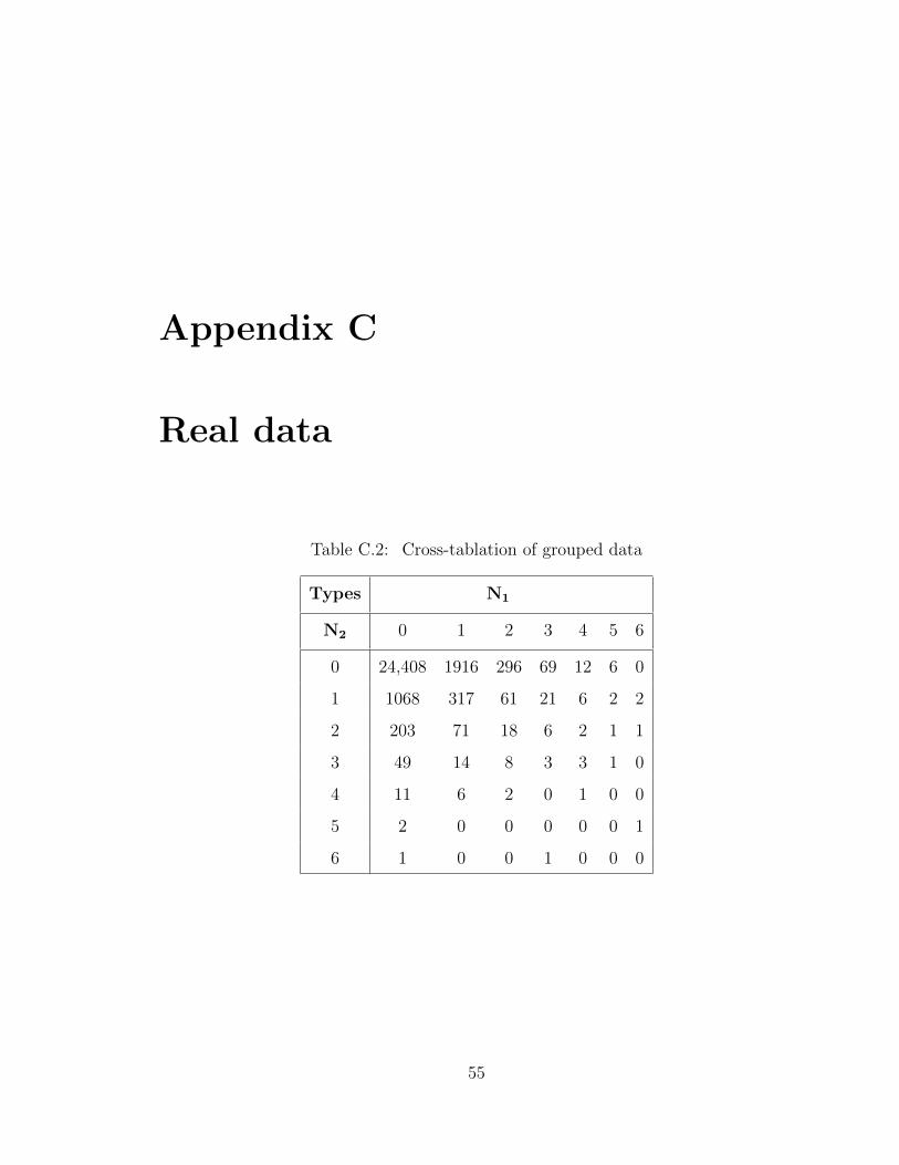
thesis. Similar to Table 1 of Bermudez and Karlis (2017), Table C.2 in Appendix C
shows the number of claims for types N1 and N2 obtained from these data. The total
number of claims is 5986. The number of claims for N1 is 3564 and for N2 is 2422.
The average frequency of N1 and N2 are 0.085 and 0.125, respectively.
4

Chapter 3
Background
In the Bivariate Conway-Maxwell-Poisson (CMP) distribution, there are three spe-
cial cases that have been mentioned in Sellers et al. (2016), which are the bivariate
Poisson, bivariate Bernoulli, and bivariate geometric distributions. The following sec-
tions focus on introducing the fundamental concepts of all four distributions starting
with the bivariate Bernoulli distribution and followed by the bivariate Poisson and
bivariate geometric distribution since they can be derived from a sequence of inde-
pendent Bernoulli random variables. Specifically, the number of failures before the
first successful results in a geometric distribution, while the number of failed trials
before the rth success has a negative binomial distribution. The Poisson distribution
can be obtained as a limit of the binomial and the negative binomial distributions.
Finally, the general theoretical framework of the bivariate CMP, that encompasses
all these three models as special cases, is described.
5

M.Sc. Thesis - Xinyi Wang McMaster - Mathematics and Statistics
3.1 Three Prominent Bivariate Distributions
3.1.1 Bivariate Bernoulli Distribution
To start from the simplest case, we recall the probability mass function of Bernoulli
random variable X is fX(x) = px(1 − p)1−x, where x is the realization of X taking
values 0 or 1. Similarly, consider another Bernoulli random variable Y . Assume they
form a random pair (X, Y ), random possessing the bivariate Bernoulli distribution
(Marshall and Olkin, 1985; Kocherlakota and Kocherlakota, 1992). Possible outcomes
of (X,Y) are (0,0), (0, 1), (1, 0), (1, 1) in the Cartesian product space {0, 1}2 =
{0, 1} × {0, 1} with probabilities p00, p01, p10 and p11 respectively.
According to the above definition of the bivariate Bernoulli distribution, it is easy
to see that the marginal distribution of X is P(X = 0) = p00 + p01 and P(X = 1) =
p10 + p11. Then X has an univariate Bernoulli distribution with parameter p10 + p11,
and Y follows another univariate Bernoulli distribution with parameter p01+p11 since
P(Y = 1) = p01 + p11 and P(Y = 0) = p00 + p10. The means of X and Y are then
p10 + p11 and p01 + p11, respectively. It is also easy to see that
Cov(X, Y ) = E(XY )− E(X)E(Y )
= p11 − (p10 + p11)(p01 + p11)
= p00p11 − p10p01,
Corr(X, Y ) = Cov(X, Y )/√p1+p0+p+1p+0
where p1+ = p10 + p11, p0+ = p00 + p01, p+1 = p01 + p11, and p+0 = p00 + p10. Due to
the close relation between probabilities, a 2 × 2 contingency table is always used to
6

M.Sc. Thesis - Xinyi Wang McMaster - Mathematics and Statistics
illustrate this distribution.
The probability mass function of a bivariate Bernoulli distribution can be written
as
P (x, y) = pxy11px(1−y)10 p
(1−x)y01 p
(1−x)(1−y)00
= exp
{log(p00) + x log
(p10p00
)+ y log
(p01p00
)+ xy log
(p11p00p10p01
)}, (3.1)
for x, y = 0, 1, where the condition p00 + p01 + p10 + p11 = 1 is satisfied. Eq. (3.1) can
be simplified using the natural parameters N ’s where
N1 = log
(p10p00
), N2 = log
(p01p00
)and N3 = log
(p11p00p10p01
)(3.2)
Then, the original mass function can be rewritten in a log-linear formulation as
P (x, y) = exp{log(p00) + x N1 + y N2 + xy N3}, (3.3)
which is a member of the exponential family of distributions.
As stated in Dai et al. (2013), the bivariate Bernoulli distribution has properties
similar to those of the bivariate Gaussian distribution. More specifically, the marginal
and conditional distributions of the bivariate Bernoulli distribution are still Bernoulli.
Finally, we have the generating function, given in Kocherlakota and Kocherlakota
(1992), as
G(t1, t2) = E(tx1 , ty2) = p00 + p01t2 + p10t1 + p11t1t2. (3.4)
7

M.Sc. Thesis - Xinyi Wang McMaster - Mathematics and Statistics
3.1.2 Bivariate Poisson Distribution
In this section, we consider the bivariate Poisson distribution which can be obtained
by taking limits in the nth power (as n→ ∞) of the factorial moment generating
function of the bivariate Bernoulli distribution; see Campbell (1934) for details.
We specifically recall the trivariate reduction method, which is a classic approach
to construct the bivariate Poisson distribution by settingX = P1+P3 and Y = P2+P3,
where independent Pi follow Poisson(λi), for i = 1, 2, 3, see Johnson et al. (1997) for
all pertinent details. It can be denoted by (X, Y ) ∼ BP (λ1, λ2, λ3), where the two
marginal distribution follows two Poisson distributions. In this case,
E(X) = λ1 + λ3,
E(Y ) = λ2 + λ3,
Cov(X, Y ) = λ3,
and Corr(X, Y ) = λ3/√
(λ1 + λ3)(λ2 + λ3)
. The correlation here is always non-negative. Further, the probability mass function
of (X, Y ) can be expressed as
P(X = x, Y = y;λ1, λ2, λ3) = e−(λ1+λ2+λ3)λx1x!
λy2y!
min(x,y)∑i=0
(x
i
)(y
i
)i!
(λ3λ1λ2
)i, (3.5)
where x and y are the realizations of X and Y , respectively. Then, we can show the
probability generating function (pgf) of the bivariate Poisson vector (X ,Y ) to be
G(t1, t2) = exp{
(λ1 + λ3)(t1 − 1) + (λ2 + λ3)(t2 − 1) + λ3(t1 − 1)(t2 − 1)}, (3.6)
8
M.Sc. Thesis - Xinyi Wang McMaster - Mathematics and Statistics
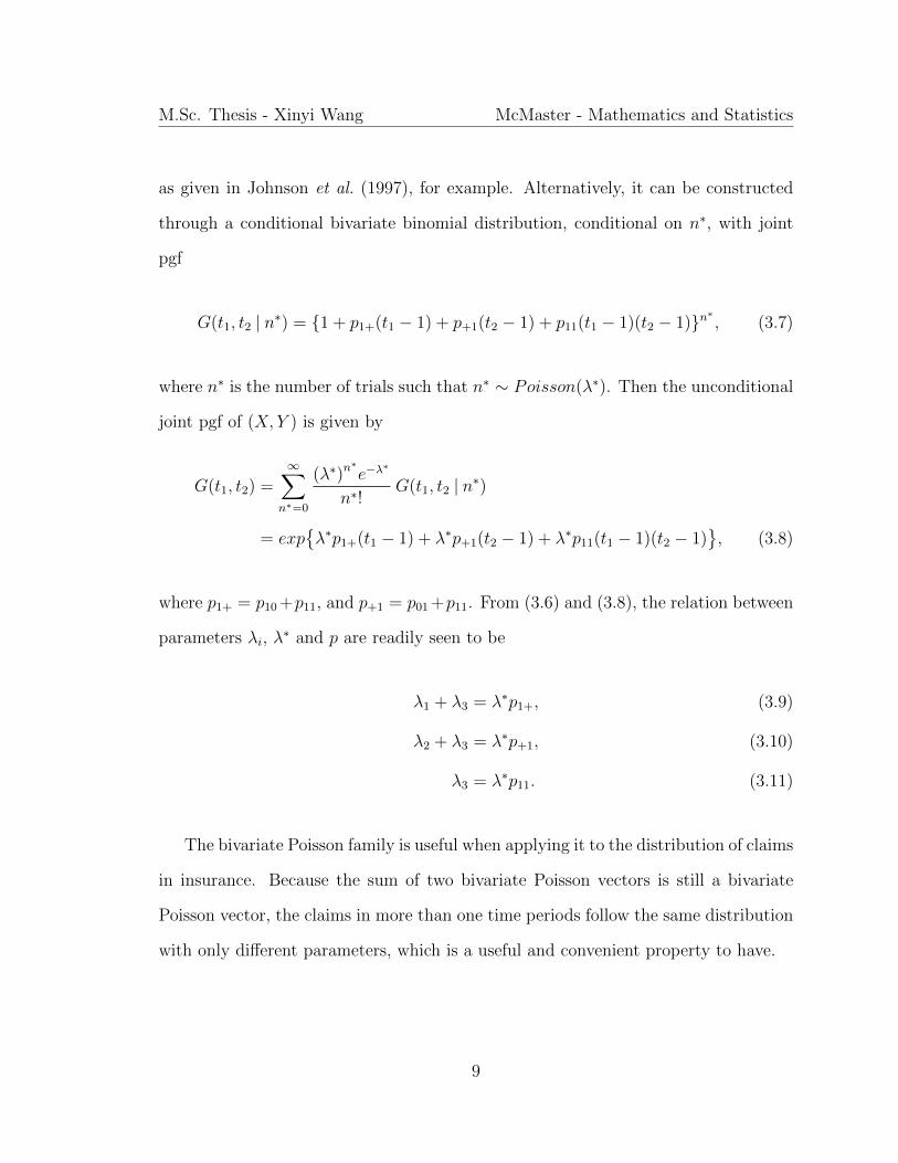
as given in Johnson et al. (1997), for example. Alternatively, it can be constructed
through a conditional bivariate binomial distribution, conditional on n∗, with joint
pgf
G(t1, t2 | n∗) = {1 + p1+(t1 − 1) + p+1(t2 − 1) + p11(t1 − 1)(t2 − 1)}n∗, (3.7)
where n∗ is the number of trials such that n∗ ∼ Poisson(λ∗). Then the unconditional
joint pgf of (X, Y ) is given by
G(t1, t2) =∞∑
n∗=0
(λ∗)n∗e−λ
∗
n∗!G(t1, t2 | n∗)
= exp{λ∗p1+(t1 − 1) + λ∗p+1(t2 − 1) + λ∗p11(t1 − 1)(t2 − 1)
}, (3.8)
where p1+ = p10+p11, and p+1 = p01+p11. From (3.6) and (3.8), the relation between
parameters λi, λ∗ and p are readily seen to be
λ1 + λ3 = λ∗p1+, (3.9)
λ2 + λ3 = λ∗p+1, (3.10)
λ3 = λ∗p11. (3.11)
The bivariate Poisson family is useful when applying it to the distribution of claims
in insurance. Because the sum of two bivariate Poisson vectors is still a bivariate
Poisson vector, the claims in more than one time periods follow the same distribution
with only different parameters, which is a useful and convenient property to have.
9

M.Sc. Thesis - Xinyi Wang McMaster - Mathematics and Statistics
3.1.3 Bivariate Geometric Distribution
Consider the bivariate geometric framework discussed in Basu and Dhar (1995). Sup-
pose a system has two components and three causes of failure which are the failure
of the first component only, failure of the second component only, and failure of
both components simultaneously. Here, the three events possess Binomial distribu-
tions with failure probabilities p1, p2, and p3, respectively, and can be denoted by
B(x, 1 − p1), B(y, 1 − p2) and B(x ∨ y, 1 − p3), where x ∨ y = max(x, y). Now con-
sider X ∈ Z+ and Y ∈ Z+ that have discrete lifetime distribution of first and second
components of the considered system. The survival function for this bivariate system
can then be expressed as
P (X > x, Y > y) = P (B(x, 1− p1) = 0, B(y, 1− p2) = 0, B(x ∨ y, 1− p3) = 0)
= px1py2pmax(x,y)3 (3.12)
and satisfies 0 < p1, p2 < 1 and 0 < p3 ≤ 1 since p1, p2 and p3 are probabilities.
Moreover, it also satisfies x ≤ 1, y ∈ Z+ where Z+ indicates positive intergers. Since
the survival function has the loss of memory property,
P (X > x+ k, Y > y + k|X > x, Y > y) = P (X > k, Y > k) = (p1 p2 p3)k,
for some positive interger k. We expend (3.12) and obtain
P (X = x, Y = y) = P (X > x− 1, Y > y − 1)− P (X > x, Y > y − 1)
−P (X > x− 1, Y > y) + P (X > x, Y > y − 1).
10

M.Sc. Thesis - Xinyi Wang McMaster - Mathematics and Statistics
It is similar as treat P (X = x, Y = y) as three cases under x < y, x = y and x > y.
P (X = x, Y = y) =
px−11 (p2p3)
y−1 (1− p1) (1− p2p3) for x < y,
(p1 p2 p3)x−1(1− p1p3 − p2p3 + p1p2p3) for x = y,
py−12 (p1p3)x−1(1− p2)(1− p1p3) for x > y.
(3.13)
The probability generating function is given by
G(t1, t2) = E(tx1 , ty2)
=∑
(x,y)∈T
tx1ty2f(x, y)
=∑x<y
tx1ty2f(x, y) +
∑x>y
tx1ty2f(x, y) +
∑x=y
tx1ty2f(x, y)
=∑x<y
tx1ty2px−11 (p2p3)
y−1q1(1− p2p3) +∑x>y
tx1ty2py−12 (p1p3)
x−1q2(1− p1p3)
+∑x=y
tx1ty2(p1p2p3)
(x− 1)(1− p1p3 − p2p3 + p1p2p3)
=t1t2q1(1− p2p3)(t2p2p3)
(1− t1t2p1p2p3)+
t1t2q2(1− p1p3)(t1p1p3)(1− t1t2p1p2p3)(1− t1p1p3)
+t1t2(1− p1p3 − p2p3 + p1p2p3)
1− t!t2p1p2p3,
where 0 < pi < 1, i = 1, 2, 3, |t1| < 1/p1, |t2| < 1/p2 and |t1t2| < 1/p1p2p3.
11

M.Sc. Thesis - Xinyi Wang McMaster - Mathematics and Statistics
3.2 Univariate Conway–Maxwell–Poisson (CMP)
Distribution
The Conway–Maxwell–Poisson (CMP) distribution is a model that naturally gener-
alizes the Poisson distribution and allows for over-dispersion and under-dispersion
in a given dataset using dispersion parameter ν. It was introduced by Conway and
Maxwell (1962), and its probability mass function is given by
P (K = k) =λk
(k!)ν1
Z(λ, ν), k = 0, 1, 2, . . . , (3.14)
where
Z(λ, ν) =∞∑i=0
λi
(i!)ν,
with ν ≥ 0, λ > 0.
The dispersion parameter ν indicates equi-dispersion when ν= 1, over-dispersion
when ν < 1, and under-dispersion when ν > 1. The CMP distribution possesses
three special cases. When ν= 1, it is a Poisson distribution with parameter λ and
in this case the dataset has equi-dispersion, and the normalizing constant becomes
Z(λ, ν) = exp(λ). Because ν → ∞ implies Z(λ, ν) → 1 + λ, the CMP in this case
becomes a Bernoulli distribution with parameter λ1+λ
. When ν = 0 and λ < 1,
it reduces a geometric distribution with success probability 1 − λ. In this case,
Z(λ, ν) =∑∞
i=0 λi = 1
1−λ is the normalizing constant, and the mass function can
be written as P(K = k;λ) = λk(1 − λ), i.e., a geometric distribution. When λ ≥ 1
and ν = 0, Z(λ, ν) does not coverage, and so in this case, the distribution is undefined.
12

M.Sc. Thesis - Xinyi Wang McMaster - Mathematics and Statistics
Moments of the CMP distribution can be derived using recursive methods since it
is from a family of two-parameter power series distribution; see Johnson et al. (1992)
for details. It has the form of
E[Kr+1] =
λE[K + 1]1−ν for r = 0,
λ∂
∂λE(Kr) + E(K)E(Kr) for r > 0.
(3.15)
The approximation of E(K) can be obtained using asymptotic approximation for the
normalizing constant Z(λ, ν). Indeed, the mean is given by
E(K) = λ∂
∂λlog(Z(λ, ν))
≈ λ1ν − ν − 1
2ν. (3.16)
Similarly, the variance, moment generating function and pgf of K are given by
V ar(K) = λ∂E(G)
∂Logλ≈ 1
νλ
1ν , (3.17)
MK(t) = E(eKt) =Z(λet, ν)
Z(λ, ν), (3.18)
GK(t) = E(tK) =Z(λt, ν)
Z(λ, ν). (3.19)
3.3 Bivariate Conway–Maxwell–Poisson (CMP) Dis-
tribution
In order to derive the distribution of the bivariate CMP distribution, we consider the
method stated in Sellers et al. (2016) which use bivariate Poisson distribution while
13

M.Sc. Thesis - Xinyi Wang McMaster - Mathematics and Statistics
the number of trials is modeled via CMP (λ, ν). Applying the compounding method
which enables us to rewrite the joint pgf of the CMP distribution along with (3.7) as
G (t1, t2) =∞∑n=0
λn
n!νZ(λ, ν)G(t1, t2|n)
=∞∑n=0
λn{1 + p1+(t1 − 1) + p+1(t2 − 1) + p11(t1 − 1)(t2 − 1)}n
n!νZ(λ, ν)(3.20)
=Z [λ{1 + p1+(t1 − 1) + p+1(t2 − 1) + p11(t1 − 1)(t2 − 1)}, ν]
Z(λ, ν)(3.21)
=1
Z(λ, ν)
∞∑n=0
1
(n!)ν(A+ Bt1 + Ct2 +Dt1t2)n (3.22)
=1
Z(λ, ν)
∞∑n=0
1
(n!)ν×W , (3.23)
where
A = λp00 = λ(1− p+1 − p1+ + p11),
B = λp10 = λ(p1+ − p11),
C = λp01 = λ(p+1 − p11),
D = λp11,
W = (A+ Bt1 + Ct2 +Dt1t2)n. (3.24)
14

M.Sc. Thesis - Xinyi Wang McMaster - Mathematics and Statistics
We use the multinomial expansion, then W has the following forms
W = (A+ Bt1 + Ct2 +Dt1t2)n
=n∑
a,b,c=0;a+d+c≤n
(n
a, b, c, n− a− b− c
)AaBbCcDn−a−b−ctn−a−c1 tn−a−b2 ,
From (3.23), if we assume x = n− a− c, y = n− a− b, the joint pmf of (X, Y ) can
be derived as P (X = x, Y = y) = 1Z(λ,ν)
∑∞n=0
λn
(n!)ν×W∗(x, y), and
W∗(x, y) =n∑
a=n−x−y
(n
a, n− a− y, n− a− x, x+ y + a− n
)pa00p
n−a−y10 pn−a−x01 px+y+a−n11 ,
as showed in Sellers et al. (2016). Its moment generating function, factorial moment
generating function, and cumulant generating function are given by
M (t1, t2) =G (et1 , et2)
=Z [λ{1 + p1+(et1 − 1) + p+1(e
t2 − 1) + p11(et1 − 1)(et2 − 1)}, ν]
Z(λ, ν),
M∗ (t1, t2) =G (t1 + 1, t2 + 1)
=Z [λ{1 + p1+t1 + p+1t2 + p11t1t2}, ν]
Z(λ, ν),
K (t1, t2) = logM (t1, t2)
=log Z [λ{1 + p1+(et1 − 1) + p+1(et2 − 1) + p11(e
t1 − 1)(et2 − 1)}, ν]− log Z(λ, ν).
Apply the knowledge of the bivariate Fisher index of dispersion, as defined in
15

M.Sc. Thesis - Xinyi Wang McMaster - Mathematics and Statistics
(Minkova and Balakrishnan, 2014),
FI(X, Y ) =
{V ar(X)
E(X)+V ar(Y )
E(Y )− 2Corr(XY )
Cov(XY )√E(Y )
√E(Y )
}(1− Corr(XY )2)−1,
we have FI(X, Y) = 2 for bivariate Poisson. Then, when ν = 1, the pgf of the CMP
distribution can be written as
G (t1, t2) = exp{λp1+(t1 − 1) + λp+1(t2 − 1) + λp11(t1 − 1)(t2 − 1)}}.
Because ν →∞, the CMP in this case is given by
G (t1, t2) = 1 + λλ+1
p1+(t1 − 1) + λλ+1
p+1(t2 − 1) + λλ+1
p11(t1 − 1)(t2 − 1).
When ν = 0 and λ < 1, it reduces a geometric distribution with success probability
1− λ. In this case, we obtain
G (t1, t2) = {1− λ
1− λ{p1+(t1 − 1) + p+1(t2 − 1) + p11(t1 − 1)(t2 − 1)}}−1,
and λ1−λ{p1+(t1−1)+p+1(t2−1)+p11(t1−1)(t2−1)} < 1. Assume the parameters of
the bivariate CMP’s are λ∗, ν∗, p∗00, p∗10, p
∗01 and p∗11. The relations between bivariate
CMP and bivariate Poisson are
p∗00 = 1− p∗11 − p∗10 − p∗01, p∗10 =λ1λ∗, p∗01 =
λ2λ∗, p∗11 =
λ3λ∗. (3.25)
The parameter values for comparison of the bivariate CMP and bivariate Bernoulli
are presented in Table B.1. The parameter values for comparison of the bivariate CMP
and bivariate Geometric distribution and the proof of this result is also presented in
Appendix B.
16
M.Sc. Thesis - Xinyi Wang McMaster - Mathematics and Statistics
The approximations perform well for λ > 10ν or ν ≤ 1. It is important to note
that CMP belongs to the exponential family, which makes the estimation easier.
There are few methods that can be used to estimate the parameters of the bivariate
CMP distribution from a dataset. Although maximum likelihood estimation (MLE)
is said to be more complex and computationally intensive for the CMP distribution,
we apply it in this thesis due to its efficiency and asymptotic properties. Details of
its application are discussed in subsequent chapters.
17

Chapter 4
Methodology
The method proposed in this thesis is the maximum likelihood estimation (MLE) for
the four models discussed in Chapter 3, and their performance are then evaluated. If
one is interested in selecting a suitable model for a given data, the selection of model
can be carried out in three ways, by applying the likelihood ratio test (LRT), by using
Akaike information criterion (AIC), or by using the Bayesian Information Criterion
(BIC). The bivariate CMP distribution includes the three special cases of bivariate
Poisson, bivariate Bernoulli, and bivariate Geometric distributions. In this work, we
denote these three special cases by M0, M1 and M2, respectively, and the bivariate
case of CMP distribution by Mg.
4.1 Maximum Likelihood Estimation (MLE)
The Maximum likelihood estimation (MLE) is a well-known method to estimate the
model parameters. The concept of MLE was first introduced by R.A. Fisher in 1920s
and has since become the most prominent model-fitting method.
18

M.Sc. Thesis - Xinyi Wang McMaster - Mathematics and Statistics
As stated in Myung (2003), let L(θ|K) be the likelihood function of a probability
distribution, where the data vector K = (k1, . . . , kn) is random sample from a pop-
ulation and the parameter vector θ is equal to (θ1, . . . , θn∗). The ML estimates are
obatined by maximizing the log-likelihood function, l(θ|K), due to the monotonicity.
If l(θ|K) is differentiable and provided that the ML estimates exist, the likelihood
equation at θi = θi is given by ∂ l(θ)/∂θi = 0 for i = 1, . . . , n∗. Note here that θi is
the MLE of parameter θi. In addition, to ensure the log-likelihood function is convex
and that θi is the maximum instead of minimum, we can check whether the second
derivative of l(θ|K) is negative, or not.
However, an optimization algorithm may generate a local maximum instead of
a global maximum depending on the choice of the starting values given for the al-
gorithm. In this thesis, different initial values were chosen over multiple iterating
processes to overcome this difficulty in the applications, discussed hereon.
4.2 MLEs for Bivariate Poisson (M0)
To compute the MLE of the bivariate Poisson, let us recall the probability function
P (x, y) in (3.5) given by
P(X = x, Y = y;λ1, λ2, λ3) = e−(λ1+λ2+λ3)λx1x!
λy2y!
min(x,y)∑i=0
(x
i
)(y
i
)i!
(λ3λ1λ2
)i.
19
M.Sc. Thesis - Xinyi Wang McMaster - Mathematics and Statistics
We now apply the recurrence relations introduced in Teicher (1954) to simplify the
calculation. It can be shown that
xP (x, y) = λ1P (x− 1, y) + λ3P (x− 1, y − 1),
yP (x, y) = λ2P (x, y − 1) + λ3P (x− 1, y − 1). (4.1)
Following the methods proposed in Holgate (1964), we take the probability mass
function of bivariate Poisson distribution in (3.5) and differentiated with respect to
λ1, λ2 and λ3 to get
∂P (x, y)
∂λ1= P (x− 1, y)− P (x, y)
∂P (x, y)
∂λ2= P (x, y − 1)− P (x, y) (4.2)
∂P (x, y)
∂λ3= P (x, y)− P (x, y − 1)− P (x− 1, y) + P (x− 1, y − 1)
Combining these with the recurrence relations for Poisson distribution given in (4.1),
the three likelihood equations∑
1P∂P (x,y)∂λ1
=∑
1P∂P (x,y)∂λ2
=∑
1P∂P (x,y)∂λ3
= 0 can be
rewritten as follows:
x
λ1− λ3λ1
W 1 − 1 = 0, (4.3)
y
λ2− λ2λ2
W 2 − 1 = 0, (4.4)
x
λ1+
y
λ2− (1 +
λ3λ1
+λ2λ2
)W 3 − 1 = 0, (4.5)
20

M.Sc. Thesis - Xinyi Wang McMaster - Mathematics and Statistics
where
W 1 =1
n
n∑i=1
P (xi − 1, yi)
P (xi, yi), (4.6)
W 2 =1
n
n∑i=1
P (xi, yi − 1)
P (xi, yi), (4.7)
and W 3 =1
n
n∑i=1
P (xi − 1, yi − 1)
P (xi, yi). (4.8)
Simplification of Eqs. (4.3)-(4.5) lead to W 1 = W 2 = W 3 = 1, which implies that
λ1 +λ3 =n∑i=1
xin
= x and λ2 +λ3 =n∑i=1
yin
= y. Therefore, the MLEs λ1, λ2 and λ3 of
the bivariate Poisson satisfies λ1 + λ3 = x and λ2 + λ3 = y. The MLEs for individual
parameters can then be estimated using an iterative process.
4.3 MLEs for Bivariate Bernoulli (M1)
One of the most important properties as mentioned in the last Chapter is that the two-
dimensional Bernoulli distribution possesses good properties similar to those of Gaus-
sian distibution as discussed in Dai et al. (2013). Recall a 2-dimensional Bernoulli
pair (X, Y ) has its probability mass function as p(x, y) = pxy11px(1−y)10 p
(1−x)y01 p
(1−x)(1−y)00 =
exp{log(p00) + x N1 + y N2 + xy N3}, as in (3.1).
In order to generate the MLE for the bivariate Bernoulli distribution, we treat
bivariate Bernoulli as a special case of the multivariate Bernoulli distribution which
21

M.Sc. Thesis - Xinyi Wang McMaster - Mathematics and Statistics
is of the form
l(x, y,N) = −ln{p(x, y)} = −{∑
x,y
(∑x≤y
Nx yC(x y)
)− b(N)
}, (4.9)
where the natural parameter is N = (N1, N2, N3)T , the interaction term C(x y) = xy,
and the normalizing factor is b(N). The normalizaing factor, also known as the log
partition function, is given by
b(N) = ln{
1 +∑x≤y
exp(N1 +N2 +N3)}
(4.10)
This is a term to ensure the disrtribution is normalized properly. Since the bivariate
Bernoulli distribution is a member of the exponential family, there are relations be-
tween the natural and general parameters. Finally, the log determinant relaxation of
the log partition function can be used to calculate the MLE of the bivariate binary
data. For details, see Banerjee et al. (2008) and Wainwright and Jordan (2006).
4.4 MLEs for Bivariate Geometric (M2)
Then, we can write the likelihood function of the bivariate Geometirc according to
Eq. (3.13) which is of the form
L(x, y ; p1, p2, p3) = pa1pb2pe3(1− p1)d(1− p2)c(1− p1p3)c
×(1− p2p3)d(1− p1p3 − p2p3 + p1p2p3)g, (4.11)
22

M.Sc. Thesis - Xinyi Wang McMaster - Mathematics and Statistics
where the letter a, b, c, d, e and g satisfied the following conditions
a =n∑i=1
(xi − n), b =n∑i=1
(yi − n),
c =n∑i=1
I[y < x], d =n∑i=1
I[x < y],
e =n∑i=1
{(y − 1)I[x < y] +
n∑i=1
(x− 1)I[x ≤ y]},
g =n∑i=1
I[x = y].
Once the formula for likelihood has been defined, the logarithm, l(x, y; p1, p2, p3), can
be passed on to find the maximum likelihood estimators p1, p2 and p3. It can be
achieved simply by solving the following score functions (Li and Dhar, 2013), where
∂l
∂p1=
a
p1− d
1− p1− cp3
1− p1p3+
g(−p3 + p2p3)
1− p1p3 − p2p3 + p1p2p3= 0, (4.12)
∂l
∂p2=
b
p2− c
1− p2− dp3
1− p2p3+
g(−p3 + p1p3)
1− p1p3 − p2p3 + p1p2p3= 0, (4.13)
∂l
∂p3=
c
p3− cp1
1− p1p3− dp2
1− p2p3+
g(−p1 − p2 + p3)
1− p1p3 − p2p3 + p1p2p3= 0. (4.14)
Due to the complex calculation involved, Eqs.(4.12) - (4.14) are not easy to solve.
Fortunately, when dataset (X, Y ) is given, the values of a, b, c, d, e, and g can be
calculated directly since they are associated with the dataset only. Given values of
a to g have been calculated, we can obtain an explicit form of the equations which
make estimation easier. Thus obtained the MLE’s for parameters p1, p2 and p3 can
be achieved through iterating process. The illustrative examples based on simulated
23

M.Sc. Thesis - Xinyi Wang McMaster - Mathematics and Statistics
datasets for this method is given in Chapter 5.
4.5 MLEs for CMP (Mg)
There are few approaches to determine the MLE for the CMP distribution as sug-
gested in Sellers and Shmueli (2010). In this thesis, we consider the method stated in
Sellers et al. (2016) which uses bivariate Poisson distribution while the number of tri-
als is modeld via CMP (λ, ν). Then according the definition of MLE, we maximize the
log-likelihood function which is given by l(λ, ν,p) =∑
x
∑y nxy lnP (X = x, Y = y).
The MLE of parameters, λ, , ν, and p, can be estimated using an iterative scheme
with deffient starting values to aviod the local maximum problem discussed before.
More details are explained in Shmueli et al. (2005).
4.6 Model Discrimination
There are a couple of criteria that have been used in this thesis for the evaluation of
parameters, the maximum likelihood estimation (MLE) and model selection. The first
model selection statistic that has been considered is the likelihood ratio test (LRT)
(King, 1998), followed by Akaike information criterion (Akaike, 1974) and Bayesian
information criterion (Schwarz, 1978).
4.6.1 Likelihood-Based Method
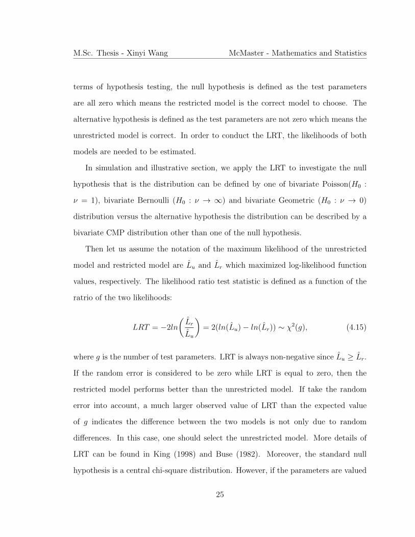
The idea of Likelihood Ratio Test (LRT) is to compare the unrestricted model and
the restricted model provided the simpler model (unrestricted model) is a special
case of the restricted model. It also called comparison of two nested models. In
24
M.Sc. Thesis - Xinyi Wang McMaster - Mathematics and Statistics
terms of hypothesis testing, the null hypothesis is defined as the test parameters
are all zero which means the restricted model is the correct model to choose. The
alternative hypothesis is defined as the test parameters are not zero which means the
unrestricted model is correct. In order to conduct the LRT, the likelihoods of both
models are needed to be estimated.
In simulation and illustrative section, we apply the LRT to investigate the null
hypothesis that is the distribution can be defined by one of bivariate Poisson(H0 :
ν = 1), bivariate Bernoulli (H0 : ν → ∞) and bivariate Geometric (H0 : ν → 0)
distribution versus the alternative hypothesis the distribution can be described by a
bivariate CMP distribution other than one of the null hypothesis.
Then let us assume the notation of the maximum likelihood of the unrestricted
model and restricted model are Lu and Lr which maximized log-likelihood function
values, respectively. The likelihood ratio test statistic is defined as a function of the
ratrio of the two likelihoods:
LRT = −2ln
(Lr
Lu
)= 2(ln(Lu)− ln(Lr)) ∼ χ2(g), (4.15)
where g is the number of test parameters. LRT is always non-negative since Lu ≥ Lr.
If the random error is considered to be zero while LRT is equal to zero, then the
restricted model performs better than the unrestricted model. If take the random
error into account, a much larger observed value of LRT than the expected value
of g indicates the difference between the two models is not only due to random
differences. In this case, one should select the unrestricted model. More details of
LRT can be found in King (1998) and Buse (1982). Moreover, the standard null
hypothesis is a central chi-square distribution. However, if the parameters are valued
25

M.Sc. Thesis - Xinyi Wang McMaster - Mathematics and Statistics
on the boundary of the parameter space, such as H0 : φ → ∞ and H0 : φ → 0, we
consider the asymptotic null distribution when conducting the LRT.
4.6.2 Information-Based Criterion
As we know that the increase of the likelihood can be achieved by increasing the pa-
rameters. In order to avoid overfitting, the Akaike information criterion (AIC, Akaike
(1974)) and Bayesian information criterion (BIC, Schwarz (1978) ) are introduced to
resolve this problem by including a term to penalize free parameters. The AIC is
defined as
AIC(θ) = −2 ln(L) + 2k, (4.16)
where L represents the value of the maximum log-likelihood of the model and k is the
number of parameters used in the model. It evaluates the performance of the models
by the goodness of fits while penalizes the increases of the parameters. The model
gives the minimum AIC value is the best model that should be selected.
The Bayesian information criterion (BIC) has been widely used as a criterion for
model selection. It is an alternative to AIC and the criterion is given by
BIC = −2 ln(L) + k ln(n), (4.17)
where L represents the value of the maximum log-likelihood for the estimated model, k
is the number of free parameters to be estimated and n is the number of observations.
The model with the lowest value of BIC is the one preferred. The increase the
variation in the dependent variable and the number of explanatory variables increase
26

M.Sc. Thesis - Xinyi Wang McMaster - Mathematics and Statistics
the value of BIC. The lower value of BIC indicates the model has few variables,
generate a better fit of the data, or both. Again, although the BIC criterion depends
on the data size n and k, it is more strict with free parameters than AIC. Also, unlike
LRT, BIC does not require the test models to be nested.
27
Chapter 5
Simulation and Illustrative
Examples
5.1 Simulation study
In the simulation study, we investigate the performance of AIC and BIC in selecting
one of the M0, M1 and M2 distribution given the true distribution is one of the three
distributions. With specified parameters, we conduct three simulated studies where
each case has data generated from one of M0, M1 and M2. Then the AIC and BIC
values have been calculated after fitted bivariate Poisson, bivariate Bernoulli, and
bivariate Geometric distribution.
Moreover, to compare the performance of bivariate Poisson and bivariate CMP
under data dispersion, we calculated AIC and BIC values of the fitted bivariate CMP
distribution to the three simulated datasets as well.
28

M.Sc. Thesis - Xinyi Wang McMaster - Mathematics and Statistics
5.1.1 Case 1
In this section, we generated a dataset with 500 data pairs that follow the bivariate
Poisson distribution (M0 model) using the rpois function in Stats package in R version
1.1.456. Applying the method of trivariate reduction discussed in Section 3.1.2, we
set Pi ∼ Poisson(λi), where the parameter λi = 1, 4, 5, X = P1+P3 and Y = P2+P3.
The range observed for X and Y are 1 to 14 and 2 to 18. The mean and variance for
X are 5.8 and 5.2, while the mean and variance for Y are 8.7 and 8.0. The empirical
dispersions are 0.9 and 0.92 for X and Y , respectively.
Table 5.1: The MLEs of bivariate Poisson and bivariate CMP models on the simulatedbivariate Poisson dataset (500 pairs)
M0 Mg
λ1 1.044 -
λ2 4.00 -
λ3 4.89 -
λ - 9.046
ν - 0.956
p00 - 0.007
p10 - 0.106
p01 - 0.401
p11 - 0.486
In Table 5.1, the generated MLEs of M0 are λ1 = 1.044, λ2 = 4.00, and λ3 = 4.89
which is close to the true values of parameters. The parameters λ and ν from CMP
distribution are 9.046 and 0.956, respectively. The ν = 9.046 indicates the simulated
29

M.Sc. Thesis - Xinyi Wang McMaster - Mathematics and Statistics
data are nearly equi-dispersion. The other four MLEs of Mg model are p00 = 0.007,
p10 = 0.106, p01 = 0.401, and p11 = 0.486. According to the formulas derived
in Section 3.2, we can calculate CMP estimates, while assuming ν ∼= 1, which are
λ1 = p10× λ = 0.959, λ2 = p01× λ = 3.627, and λ3 = p11× λ = 4.993. It is clear that
the estimates of the bivariate Poisson distribution are close to the true values under
M0.
Then, we fit the dataset to M0, M1, M2 and Mg and resulting values of log-
likelihood and AIC are presented in Table 5.2. The log-likelihood of M0 and Mg are
similar. However, according to the AIC and BIC formulas in Section 3.2, AIC, and
BIC of M0 are lower than those of Mg due to lower penalty based on the number of
parameters. The likelihood ratio test confirms that the data are from M0 model since
LRT = −2ln(L∗) = 0.40 with a p-value of 0.53, where L∗ = LrLu
.
Table 5.2: The Log-likelihood, AIC and BIC of bivariate Poisson(M0), bivariateBernoulli (M1), bivariate Geometric (M2) and bivariate CMP (Mg) models on thesimulated bivariate Poisson dataset (500 pairs)
M0 M1 M2 Mg
LnL -2259.120 -2833.026 -2828.070 -2258.919
AIC 4524.240 5674.052 5662.130 4525.838
BIC 4536.884 5641.194 5674.774 4542.696
5.1.2 Case 2
In the second case of our simulation study, we used rbinom2.or in package VGAM in
R to generate 500 data pairs from a bivariate Bernoulli model (M1). We set the
30

M.Sc. Thesis - Xinyi Wang McMaster - Mathematics and Statistics
marginal probability for the first component to be 0.6, odds ratio equal to exp(1.5)
and the two marginal probabilities are constrained to be equal. The dataset has zeros
and ones with means of X and Y as 0.63 and 0.64, variances as 0.23 and 0.24, and the
empirical dispersions are 0.37 and 0.40, respectively. It is equivalent to generating a
dataset with probabilities p00 = 0.244, p01 = 0.156, p10 = 0.156, and p11 = 0.444.
Table 5.3: The MLEs of bivariate Poisson (M0) and bivariate CMP (Mg) models onthe simulated bivariate Bernoulli dataset (500 pairs)
M0 Mg
λ1 0.158 -
λ2 0.202 -
λ3 0.410 -
λ - 6.000
ν - 30.000
p00 - 0.153
p10 - 0.306
p01 - 0.268
p11 - 0.273
In this case, as shown in Table 5.3, the estimates λ and ν of Mg are 6 and 30 with
p00 = 0.153, p10 = 0.306, p01 = 0.268, and p11 = 0.273. The under dispersion in the
data is naturally detected by the estimate ν = 30. According to the relation between
Mg and M1, the estimated probabilities of the bivariate Bernoulli, as a special case
31

M.Sc. Thesis - Xinyi Wang McMaster - Mathematics and Statistics
of the CMP distribution, are given by
p∗00 = 1− λ
λ+ 1(p01 + p10 + p11) ∼= 0.232, (5.1)
p∗01 =λ
λ+ 1p01 ∼= 0.133, (5.2)
p∗10 =λ
λ+ 1p10 ∼= 0.163, (5.3)
p∗11 =λ
λ+ 1p11 ∼= 0.469. (5.4)
Compare results from (5.1) - (5.4) with true probabilities of the data. We noticed
that p00 and p01 are slightly underestimated by the second decimal place and p10 and
p11 are slightly overestimated . In general, the overall estimation is quite accurate
since 1− µ = 0.4, and p∗00 + p∗10 = 0.394.
Table 5.4: The Log-likelihood, AIC and BIC of bivariate Poisson (M0), bivariateBernoulli (M1), and bivariate CMP (Mg) models on the simulated bivariate Bernoullidataset (500 pairs)
M0 M1 Mg
LnL -831.110 -629.819 -629.819
AIC 1668.220 1265.638 1267.638
BIC 1680.864 1278.282 1284.496
TheM1 generates the lowest AIC and BIC values amongM0,M1, andMg. In Table
5.4, the difference in AIC values are small for Mg and M1 while M1’s value is slightly
lower. We performed likelihood ratio test between M0 and Mg with −2ln(L∗) ∼= 403
and a p-value around 0, which indicates M0 is not the correct model and the existence
of significant data dispersion. Again, the LRT between Mg and M1 confirms that the
32

M.Sc. Thesis - Xinyi Wang McMaster - Mathematics and Statistics
simulated data is from M1 model since −2ln(L∗) ∼= 0 with p-value greater than
significance level. Thus, the bivariate CMP model detects the under-dispersion in the
data, and provides a better fit.
5.1.3 Case 3
For the third case, we used rbivgeo2 in package BivGeo in R to generate 500 data pairs
from a bivariate Geometric model (M2). We set failure probabilities equal to 0.9. The
ranges for X and Y are 1 to 21 and 1 to 20, with means 3.12 to 3.73, and variances
7.00 and 10.25, respectively. The empirical dispersions are 2.24 and 2.75. Applying
the method as in pervious cases, as shown in Table 5.5, the MLEs for M0 model are
λ1 = 1.92, λ2 = 2.53, λ3 = 1.2, the MLE for Mg model are λ = 0.942, ν = 0.000,
p00 = 0.389, p01 = 0.339, p10 = 0.270, and p11 = 0.002. Dispersion parameter here is
smaller than 1, which implies that the data are over-dispersion.
Table 5.5: The MLEs of bivariate Poisson (M0) and bivariate CMP (Mg) models onthe simulated bivariate Geometric dataset (500 pairs)
M0 Mg
λ1 1.920 -
λ2 2.530 -
λ3 1.200 -
λ - 0.942
ν - 0.000
p00 - 0.389
p10 - 0.339
p01 - 0.270
p11 - 0.002
33

M.Sc. Thesis - Xinyi Wang McMaster - Mathematics and Statistics
Model M2 generates the lowest AIC and BIC values among M0,M2, and Mg. From
Table 5.6, the log-likelihood value for Mg ( ∼= −2583.909) is significantly larger than
the log-likelihood value for M0 ( ∼= −3142.720). It can also be shown by LRT where
−2ln(L∗) = 1117.622 with p-value significantly small (∼= 0). It implies the existence
of data dispersion and M0 is not the correct model to use. Moreover, Mg generated
the smaller AIC and BIC value than M0 model in this case.
Again, the LRT between Mg and M1 confirms that the simulated data is from
M1 model since −2ln(L∗) ∼= 1.242 with a p-value of 0.265. Here again, the bivariate
CMP model outperforms the bivariate Poisson model by considering the dispersion
in the data.
Table 5.6: The Log-likelihood, AIC and BIC of bivariate Poisson (M0), bivariate Ge-ometric (M2), and bivariate CMP (Mg) models on the simulated bivariate Geometricdataset (500 pairs)
M0 M2 Mg
LnL -3142.720 -2584.530 -2583.909
AIC 6291.442 5175.060 5175.818
BIC 6304.255 5187.704 5192.676
From the previous three cases with different dispersion of the datasets, we ob-
serve that the bivariate CMP always outperforms the bivariate Poisson model if data
dispersion is presented. It is agreed with the theoretical derivation as in Chapter 4.
34

M.Sc. Thesis - Xinyi Wang McMaster - Mathematics and Statistics
5.1.4 Illustrative real data analysis
In this section, we compare and contrast the performance of the bivariate Poisson
model and the CMP model using the data introduced in Chapter 2. According to
Bermudez and Karlis (2017), the bivariate Poisson model is approved to perform well
with the auto insurance data. In this section, we fit the data using the CMP model
while monitoring data dispersion using the dispersion parameter ν.
Recall X and Y are annual number of claims for N1 type and N2 type, respectively.
We observed values of X and Y with ranges of 1-6 and 1-6, means of 0.085 and 0.125,
variances of 0.130 and 0.178, and empirical dispersions are 1.5 and 1.4. Fitting M0
model produces parameters λ1 = 0.04, λ2 = 0.5 and λ3 = 1.13. The MLEs for the
Mg model are λ = 0.112, ν = 0.000, p00 = 0.011, p01 = 0.315, p10 = 0.001, and
p11 = 0.672, as shown in Table 5.7. Here, the dispersion parameter is equal to zero,
which indicates that the data are over-dispersed.
Table 5.7: The MLEs of bivariate Poisson (M0) and bivariate CMP (Mg) models onthe automobile insurance dataset
M0 Mg
λ1 0.040 -
λ2 0.500 -
λ3 1.130 -
λ - 0.112
ν - 0.000
p00 - 0.011
p10 - 0.001
p01 - 0.315
p11 - 0.672
35

M.Sc. Thesis - Xinyi Wang McMaster - Mathematics and Statistics
Table 5.8: The Log-likelihood, AIC and BIC of bivariate Poisson (M0), and bivariateCMP (Mg) models on the automobile insurance dataset
bivariate Poisson (M0) bivariate CMP (Mg)
LnL -13690.590 -13303.180
AIC 27387.180 26614.360
BIC 27411.867 26647.403
From Table 5.8, the log-likelihood for Mg is -13303.180, which is larger than the
value for M0. When the Mg model is fitted to the data, it produces lower AIC value
than when the M0 model is fitted (AICMg = 26614 < AICM0 = 27387). So, Mg
outperforms M0 based on AIC. We then compare the BIC values of the two models.
The BIC for M0 and Mg are 27412 and 26617, respectively. Based on these BIC
values, we find that the CMP model fit the data better than the bivariate Poisson
model.
When we apply the LRT to M0 and Mg, we also notice that −2ln(L∗) ∼= 774.820
with a p-value of 1.610× 10−170. Hence, we reject the null hypothesis of the bivariate
Poisson. Since the data are over-dispersed, we tried to fit it using a negative bivariate
binomial model which is a more general form of the bivariate geometric distribution,
and it has log-likelihood value, AIC, and BIC of -13365.810, 26762.400, 26762.400.
Although its values show the model performs better than bivariate Poisson, the bi-
variate CMP still provides the best model among these.
These examples demonstrate that the bivariate CMP model outperforms the bi-
variate Poisson for modeling the auto insurance dataset given by Bermudez and Karlis
(2017) due to the presence of dispersion in the data.
36

Chapter 6
Conclusions and Future Work
In this thesis, we have demonstrated the usefulness of the CMP model as a more gen-
eral case of the bivariate Poisson distribution. It closely monitors the over and under
dispersion for bivariate count data which allows the analysis to be more accurate.
As a more general model, the CMP captures bivariate Poisson, bivariate Bernoulli
and bivariate geometric as three special cases, and can be used as a tool for analyzing
other structure using its dispersion parameter. We have applied the theoretical frame-
work to the simulation study and real data from an insurance company in Chapter 5.
The results fully demonstrated bivariate CMP is a powerful overarching model with
lower AIC, BIC values than bivariate Poisson model with and without data disper-
sion. Along with model discrimination, we also performed parameter estimation and
hypothesis testing for simulated and real datasets.
As a powerful model, the bivariate CMP distribution has ensured a more general
model fitting results. However, as a complex distribution, it does not have a closed-
form. Because of the complexity of its calculation, the difficulty of applying it raises.
37

M.Sc. Thesis - Xinyi Wang McMaster - Mathematics and Statistics
In this work, we have used the R package from Sellers et al. (2018) where it uses
the finite sum to approximate the distribution. Although it is a relatively reliable
approach, more research has to be done to reveal the impact of infinite summation to
the iterating process when generating the bivariate CMP model. The goodness of fit
tests and Bayesian inference can also be performed. The extension of bivariate CMP
to multivariate CMP is another topic can be focused on. Its accuracy of modeling
can be investigated if the dataset has been grouped into more than two categories.
38
Appendix A
R code
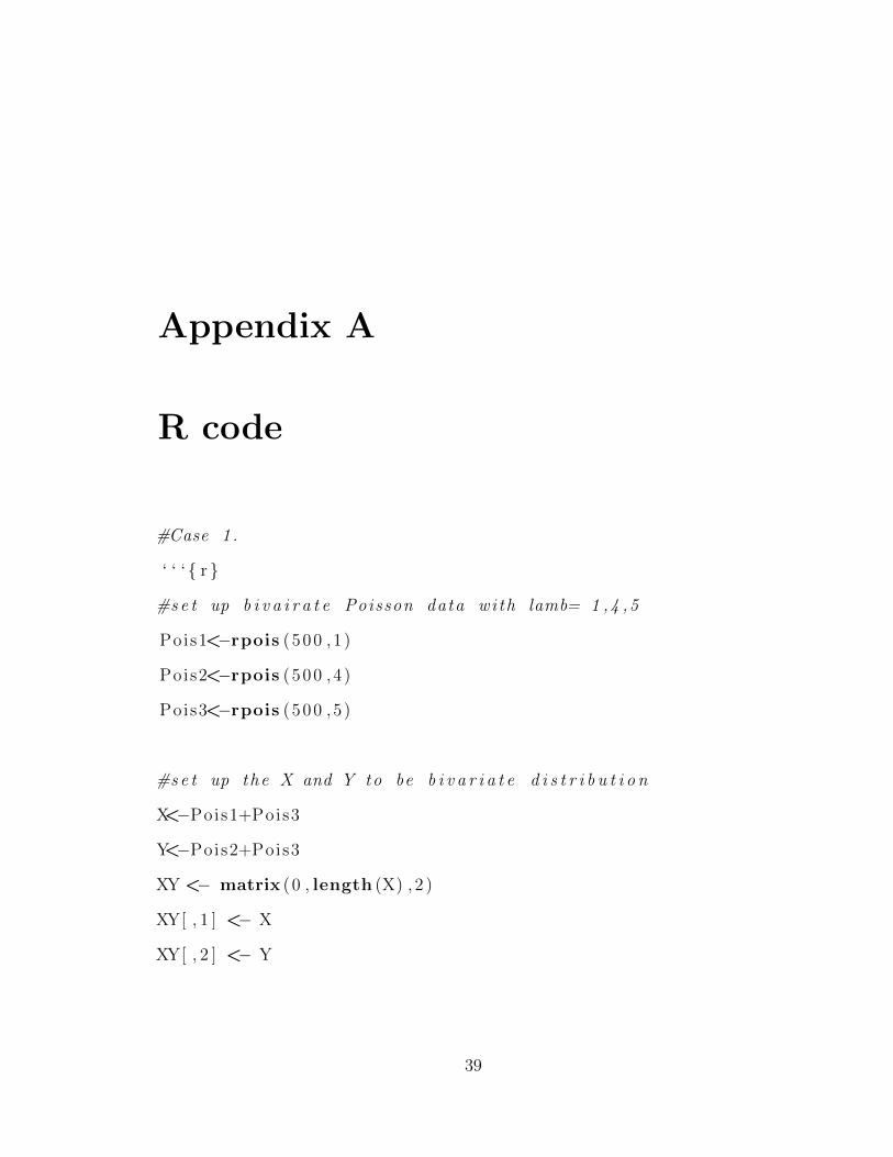
#Case 1 .
‘ ‘ ‘{ r}
#se t up b i v a i r a t e Poisson data wi th lamb= 1 ,4 ,5
Pois1<−rpois (500 ,1 )
Pois2<−rpois (500 ,4 )
Pois3<−rpois (500 ,5 )
#se t up the X and Y to be b i v a r i a t e d i s t r i b u t i o n
X<−Pois1+Pois3
Y<−Pois2+Pois3
XY <− matrix (0 , length (X) , 2 )
XY[ , 1 ] <− X
XY[ , 2 ] <− Y
39
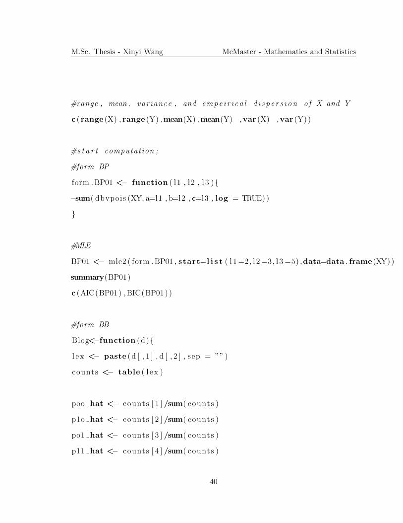
M.Sc. Thesis - Xinyi Wang McMaster - Mathematics and Statistics
#range , mean , variance , and empe i r i ca l d i s p e r s i on o f X and Y
c ( range (X) , range (Y) ,mean(X) ,mean(Y) ,var (X) ,var (Y) )
#s t a r t computation ;
#form BP
form . BP01 <− function ( l1 , l2 , l 3 ){
−sum( dbvpois (XY, a=l1 , b=l2 , c=l3 , log = TRUE) )
}
#MLE
BP01 <− mle2 ( form . BP01 , start=l i s t ( l 1 =2, l 2 =3, l 3 =5) ,data=data . frame (XY) )
summary(BP01)
c (AIC(BP01) ,BIC(BP01 ) )
#form BB
Blog<−function (d){
l e x <− paste (d [ , 1 ] , d [ , 2 ] , sep = ”” )
counts <− table ( l ex )
poo hat <− counts [ 1 ] /sum( counts )
p1o hat <− counts [ 2 ] /sum( counts )
po1 hat <− counts [ 3 ] /sum( counts )
p11 hat <− counts [ 4 ] /sum( counts )
40

M.Sc. Thesis - Xinyi Wang McMaster - Mathematics and Statistics
props <− c ( poo hat , p1o hat , po1 hat , p11 hat )
L <− sum( counts∗log ( props ) )
return (L)
}
#MLE BB
Blog (XY)
(−2)∗Blog (XY)+2∗4 #AIC.BB
(−2)∗Blog (XY)+2∗log (500)#BIC .BB
#log pmg o f BG
dbg<−function (x , p = c ( ) ) {
x<−as .matrix ( x )
x0 <− x [ , 1 ]
y0 <− x [ , 2 ]
i n t e r 1 <− p [ 1 ] ∗ p [ 3 ]
i n t e r 2 <− p [ 2 ] ∗ p [ 3 ]
i n t e r 3 <− p [ 1 ] ∗ p [ 2 ] ∗ p [ 3 ]
#x<y
t e r 1 <− p [ 1 ] ˆ ( x0 − 1) ∗ ( i n t e r 2 )ˆ ( y0 − 1)
t e r2 <− (1 − i n t e r 2 ) ∗ (1 − p [ 1 ] )
f o r 1 <− t e r 1 ∗ t e r 2
#x=y
41

M.Sc. Thesis - Xinyi Wang McMaster - Mathematics and Statistics
t e r 3 <− ( i n t e r 3 )ˆ ( x0 − 1)
t e r4 <− (1 − i n t e r 1 − i n t e r 2 + i n t e r 3 )
f o r 2 <− t e r 3 ∗ t e r 4
#x>y
t e r 5 <− p [ 2 ] ˆ ( y0 − 1) ∗ ( i n t e r 1 )ˆ ( x0 − 1)
t e r6 <− (1 − i n t e r 1 ) ∗ (1 − p [ 2 ] )
f o r 3 <− t e r 5 ∗ t e r 6
pmf .BG <− i f e l s e ( x0 < y0 , for1 ,
i f e l s e ( x0 > y0 , for3 , f o r 2 ) )
return ( log (pmf .BG) )
}
#form BG
form . BG01 <− function ( t1 , t2 , t3 ){
f<−dbg (XY, p=c ( t1 , t2 , t3 ) )
return(−sum( as .numeric ( f ) ) )
}
#MLE BG
BG01 <− mle2 ( form . BG01 , start=l i s t ( t1 =0.5 , t2 =0.5 , t3 =0.7) ,data=data . frame (XY) , method = ” Nelder−Mead” )
summary(BG01)
c (AIC(BG01) ,BIC(BG01) )
#MLE CMP
42

M.Sc. Thesis - Xinyi Wang McMaster - Mathematics and Statistics
COM.MLE.BP<−mult icmpests (XY, s t a r t v a l u e s = c (9 , 1 , 0 , 0 . 1 , 0 . 4 , 0 . 5 ) )
#check i f the lambda c a l c u l a t e d base on parameters genera ted from COM model i s c l o s ed to the o r i g i n a l lambda va l u e s ;
e s t . l 1<−COM.MLE.BP$par [ 1 ] ∗COM.MLE.BP$par [ 5 ]
e s t . l 2<−COM.MLE.BP$par [ 1 ] ∗COM.MLE.BP$par [ 4 ]
e s t . l 3<−COM.MLE.BP$par [ 1 ] ∗COM.MLE.BP$par [ 6 ]
( 2 )∗(COM.MLE.BP$ n e g l l )+2∗6 #AIC CMP
(2 )∗(COM.MLE.BP$ n e g l l )+6∗log (500) #BIC CMP
##Case 2 .
#genera te BB data
BB. data<−rbinom2 . or (500 ,mu1=0.6 , o r a t i o=exp ( 1 . 5 ) , exchangeable = TRUE)
#check i n i t i a l v a l u e s o f p [ i j ]
dbinom2 . or (mu1=0.6 , exchangeable = TRUE, o r a t i o = exp ( 1 . 5 ) )
BB. data<−as .matrix (BB. data0 )
range (BB. data [ , 1 ] )
range (BB. data [ , 2 ] )
mean(BB. data [ , 1 ] )
mean(BB. data [ , 2 ] )
var (BB. data [ , 1 ] )
43

M.Sc. Thesis - Xinyi Wang McMaster - Mathematics and Statistics
var (BB. data [ , 2 ] )
#s t a r t computation ;
#form BP
BP2 <− function ( l1 , l2 , l 3 ){
−sum( dbvpois (BB. data , a=l1 , b=l2 , c=l3 , log = TRUE) )
}
#MLE BP
BP02 <− mle2 (BP2, start=l i s t ( l 1 =0.1 , l 2 =0.03 , l 3 =0.3) ,data=data . frame (BB. data ) , method = ” Nelder−Mead” )
summary(BP02)
AIC(BP02)
BIC(BP02)
#MLE BB
Blog (BB. data )
(−2)∗Blog (BB. data)+2∗4 #AIC.BB
(−2)∗Blog (BB. data)+2∗log (500)#BIC .BB
#form BG
BG2 <− function ( t1 , t2 , t3 ){
f<−dbg (BB. data , p=c ( t1 , t2 , t3 ) )
return(−sum( as .numeric ( f ) ) )
}
#MLE BG
44

M.Sc. Thesis - Xinyi Wang McMaster - Mathematics and Statistics
BG02 <− mle2 (BG2, start=l i s t ( t1 =0.5 , t2 =0.5 , t3 =0.5) ,data=data . frame (BB. data ) , method = ” Nelder−Mead” )
summary(BG02)
c (AIC(BG02) ,BIC(BG02) )
#MLE CMP
COM.MLE.BB<−mult icmpests (BB. data , s t a r t v a l u e s = c (6 , 30 , 0 . 2 , 0 . 1 , 0 . 1 , 0 . 6 ) )
(2 )∗(COM.MLE.BB$ n e g l l )+2∗6 #AIC
(2 )∗(COM.MLE.BB$ n e g l l )+6∗log (500) #BIC
##Case 3 .
#data
G<−rb ivgeo1 (500 , theta=c ( 0 . 8 4 , 0 . 9 1 2 , 0 . 8 1 4 ) )
G<−as .matrix (G)
c ( range (G[ , 1 ] ) , range (G[ , 2 ] ) ,mean(G[ , 1 ] ) ,mean(G[ , 2 ] ) , var (G[ , 1 ] ) , var (G[ , 2 ] ) )
BP3 <− function ( l1 , l2 , l 3 ){
−sum( dbvpois (G, a=l1 , b=l2 , c=l3 , log = TRUE) )
}
BP03 <− mle2 (BP3, start=l i s t ( l 1 =10, l 2 =10, l 3 =1) ,data=data . frame (G) , method = ” Nelder−Mead” )
#−3488.5
AIC(BP03)
45

M.Sc. Thesis - Xinyi Wang McMaster - Mathematics and Statistics
BIC(BP03)
BG3 <− function ( t1 , t2 , t3 ){
f<−dbg (G, p=c ( t1 , t2 , t3 ) )
return(−sum( as .numeric ( f ) ) )
}
#MLE
BG03 <− mle2 (BG3, start=l i s t ( t1 =0.9 , t2 =0.9 , t3 =0.9) ,data=data . frame (G) , method = ” Nelder−Mead” )
summary(BG03)
AIC(BG03)
BIC(BG03)
#MLE CMP
COM.MLE.BG<−mult icmpests (G, s t a r t v a l u e s = c (1 , 0 , 0 , 0 . 4 , 0 . 4 , 0 . 2 ) )
(2 )∗(COM.MLE.BG$ n e g l l )+2∗6
(2 )∗(COM.MLE.BG$ n e g l l )+6∗log (20)
##Real Data .
#data
x0<−c (24408 ,1916 ,296 ,69 ,12 ,6 ,0 )
x1<−c (1068 , 317 , 61 ,21 ,6 , 2 ,2 )
46

M.Sc. Thesis - Xinyi Wang McMaster - Mathematics and Statistics
x2<−c (203 , 71 , 18 , 6 ,2 , 1 , 1)
x3<−c ( 49 , 14 , 8 , 3 , 3 , 1 , 0 )
x4<−c (11 , 6 , 2 , 0 , 1 , 0 ,0 ,0 )
x5<−c (2 ,0 ,0 , 0 ,0 , 0 , 1)
x6<−c ( 1 , 0 , 0 , 1 , 0 , 0 , 0 )
x8<−c ( 0 , 0 , 1 , 0 , 0 , 0 , 0 )
DR<−rbind ( x0 , x1 , x2 , x3 , x4 , x5 , x6 , x8 )
#N1: s i n g l e row sum
f r<−function ( x ){
sum(DR[ x , 1 : 7 ] )
}
sum. 1<−rbind ( f r ( 1 ) , f r ( 2 ) , f r ( 3 ) , f r ( 4 ) , f r ( 5 ) , f r ( 6 ) , f r ( 7 ) , f r ( 8 ) )
#N2: s i g n l e c o l sum
f c<−function ( x ){
sum(DR[ 1 : 8 , x ] )
}
sum. 2<−cbind ( f c ( 1 ) , f c ( 2 ) , f c ( 3 ) , f c ( 4 ) , f c ( 5 ) , f c ( 6 ) , f c ( 7 ) )
#check i f N1=N2?
sum(sum.1)−sum(sum . 2 )
#t o t a l o b s e r va t i on s : 28590
#func to genera t ing N1 vec to r
N1 . f<−function ( x ){
47

M.Sc. Thesis - Xinyi Wang McMaster - Mathematics and Statistics
rep (x , t imes=sum . 1 [ x+1])
}
#func to genera t ing N2 vec to r
N2 . f<−function ( y ){
rep (y , t imes=sum . 2 [ y+1])
}
N1<−c (N1 . f ( 0 ) ,N1 . f ( 1 ) ,N1 . f ( 2 ) ,N1 . f ( 3 ) ,N1 . f ( 4 ) ,N1 . f ( 5 ) ,N1 . f ( 6 ) , rep (8 , time=1))
N2<−c (N2 . f ( 0 ) ,N2 . f ( 1 ) ,N2 . f ( 2 ) ,N2 . f ( 3 ) ,N2 . f ( 4 ) ,N2 . f ( 5 ) ,N2 . f ( 6 ) )
DR. b i<−cbind (N1 , N2)
#dim(DR. b i )
as .matrix (DR. b i )
#mean , var iance and d i s p e r s i on o f N1 and N2
c (mean(DR. b i [ , 1 ] ) ,mean(DR. b i [ , 2 ] ) ,var (DR. b i [ , 1 ] ) ,var (DR. b i [ , 2 ] ) )
#s t a r t computat ions ;
#form BP
f . br <− function ( l1 , l2 , l 3 ){
−sum( dbg (DR. bi , a=l1 , b=l2 , c=l 3 )
}
#MLE
48

M.Sc. Thesis - Xinyi Wang McMaster - Mathematics and Statistics
BP. r <− mle2 ( f . br , start=l i s t ( l 1 =0.09 , l 2 =0.11 , l 3 =0.01) ,data=data . frame (DR. b i ) , method=” Nelder−Mead” )
summary(BP. r )
#MLE CMP
COM. dr<−mult icmpests (DR. bi , s t a r t v a l u e s = c (1 , 1 , 0 . 25 , 0 . 25 , 0 . 25 , 0 . 2 5 ) )
D1<−(2 )∗(COM. dr$ n e g l l )+2∗6 #AIC
D2<−(2 )∗(COM. dr$ n e g l l )+6∗log (28590) #BIC
c (AIC(BP. r ) ,BIC(BP. r ) ,D1 , D2)
49

Appendix B
Derivation of the three special
cases via pgf
Similar as Section 4.5, we consider the method stated in Sellers et al. (2016) which use
bivariate Poisson distribution while the number of trials is modelled via CMP (λ, ν).
Applying the compounding method which enables us to rewrite the joint pgf of the
CMP distribution along with (3.7) as
G (t1, t2) =∞∑n=0
λn
n!νZ(λ, ν)G(t1, t2|n)
=∞∑n=0
λn{1 + p1+(t1 − 1) + p+1(t2 − 1) + p11(t1 − 1)(t2 − 1)}n
n!νZ(λ, ν)
=Z [λ{1 + p1+(t1 − 1) + p+1(t2 − 1) + p11(t1 − 1)(t2 − 1)}, ν]
Z(λ, ν)(B.1)
50
M.Sc. Thesis - Xinyi Wang McMaster - Mathematics and Statistics
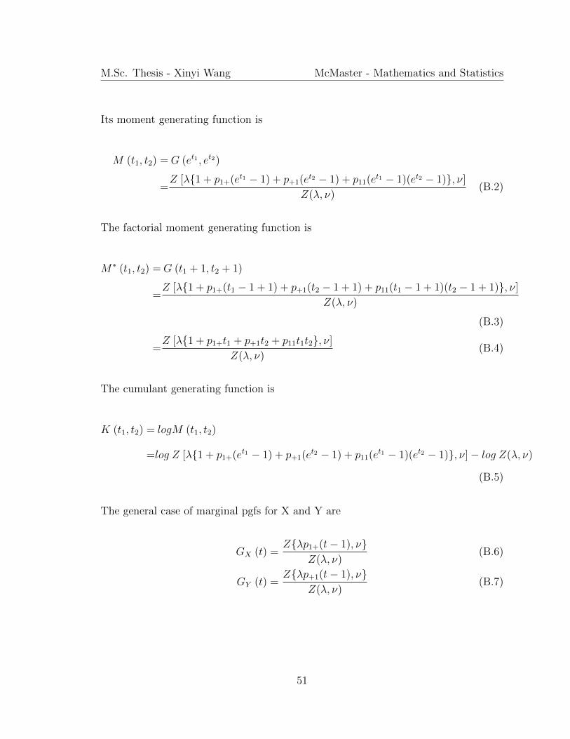
Its moment generating function is
M (t1, t2) =G (et1 , et2)
=Z [λ{1 + p1+(et1 − 1) + p+1(e
t2 − 1) + p11(et1 − 1)(et2 − 1)}, ν]
Z(λ, ν)(B.2)
The factorial moment generating function is
M∗ (t1, t2) =G (t1 + 1, t2 + 1)
=Z [λ{1 + p1+(t1 − 1 + 1) + p+1(t2 − 1 + 1) + p11(t1 − 1 + 1)(t2 − 1 + 1)}, ν]
Z(λ, ν)
(B.3)
=Z [λ{1 + p1+t1 + p+1t2 + p11t1t2}, ν]
Z(λ, ν)(B.4)
The cumulant generating function is
K (t1, t2) = logM (t1, t2)
=log Z [λ{1 + p1+(et1 − 1) + p+1(et2 − 1) + p11(e
t1 − 1)(et2 − 1)}, ν]− log Z(λ, ν)
(B.5)
The general case of marginal pgfs for X and Y are
GX (t) =Z{λp1+(t− 1), ν}
Z(λ, ν)(B.6)
GY (t) =Z{λp+1(t− 1), ν}
Z(λ, ν)(B.7)
51

M.Sc. Thesis - Xinyi Wang McMaster - Mathematics and Statistics
For the Poisson case, set ν = 1, then marginal pgfs for X and Y are
G∗X (t; ν = 1) = exp {λp1+(t− 1)} ∼ Poisson(λp+1) (B.8)
G∗Y (t; ν = 1) = exp {λp+1(t− 1)} ∼ Poisson(λp1+) (B.9)
When ν = 1 pgf of (X, Y) becomes (3.8)
G (t1, t2) = exp{λ[1 + p1+(t1 − 1) + p+1(t2 − 1) + p11(t1 − 1)(t2 − 1)]− λ} (B.10)
= exp{λp1+(t1 − 1) + λp+1(t2 − 1) + λp11(t1 − 1)(t2 − 1)}}
and the relations between parameters of trivariate reduction method and the param-
eters from CMP are
λ1 + λ3 = λp1+
λ2 + λ3 = λp+1
λ3 = λp11
For the bivariate Bernoulli, set ν →∞, and then pgf of (X, Y) becomes
G (t1, t2) =1 + λ{1 + p1+(t1 − 1) + p+1(t2 − 1) + p11(t1 − 1)(t2 − 1)}
1 + λ
=1 +λ
λ+ 1p1+(t1 − 1) +
λ
λ+ 1p+1(t2 − 1) +
λ
λ+ 1p11(t1 − 1)(t2 − 1)
(B.11)
compare the (B.11) and (3.4), we generate the relation between parameters of bivari-
ate Bernoulli and the Bernoulli case under the CMP model. The details are in Table
52

M.Sc. Thesis - Xinyi Wang McMaster - Mathematics and Statistics
Table B.1: The probability table of bivariate Bernoulli distribution as a special caseof CMP distribution as ν →∞
Y
X
0 1
0 p∗00 = 1− λλ+1
(p01 + p10 + p11) p∗01 = λλ+1
p01 p∗0+ = 1− λ1+λ
p1+
1 p∗10 = λ1+λ
p10 p∗11 = λ1+λ
p11 p∗1+ = λ1+λ
p1+
p∗+0 = 1− λ1+λ
p+1 p∗+1 = λ1+λ
p+1
B.1.
For the Geometric case, when ν = 0, λ < 1 the Z(λ, ν) = 11−λ . The pgf becomes
a bivariate Geometric distribution as
G (t1, t2) =1− λ
1− λ{1 + p1+(t1 − 1) + p+1(t2 − 1) + p11(t1 − 1)(t2 − 1)}(B.12)
=1
1− λ1−λ{p1+(t1 − 1) + p+1(t2 − 1) + p11(t1 − 1)(t2 − 1)}
(B.13)
for both numerator and denominator of (B.12) are greater than 0. It is similar as
set α as an exp(θ) with probability density function as f(α) = 1θe−α/θ to the pgf of
Poisson case, where θ > 0 and α > 0. Recall the pgf of a bivariate poisson as in
(B.10) where G (t1, t2) = exp{αc1(t1 − 1) + αc2(t2 − 1) + αc3(t1 − 1)(t2 − 1)}. Then
53

M.Sc. Thesis - Xinyi Wang McMaster - Mathematics and Statistics
combine adjusted (B.10), the unconditional joint pfg of (X, Y ) is
G (t1, t2) =
∫ ∞0
G (t1, t2 | α)f(α)dα
=
∫ ∞0
1
θe−α[
1θ−c1(t1−1)−c2(t2−1)−c3(t1−1)(t2−1)] dα
=1/θ
1/θ − [c1(t1 − 1) + c2(t2 − 1) + c3(t1 − 1)(t2 − 1)]
=1
1− θ[c1(t1 − 1) + c2(t2 − 1) + c3(t1 − 1)(t2 − 1)]](B.14)
where the denominator of (B.14) is great than 0. Hence, compare (B.11) and (B.14),
the relations between parameter of bivariate Geometric and as a special case of the
bivariate CMP are
θc1 =λ
1− λp1+, θc2 =
λ
1− λp+1, θc3 =
λ
1− λp11.
54
Appendix C
Real data
Table C.2: Cross-tablation of grouped data
Types N1
N2 0 1 2 3 4 5 6
0 24,408 1916 296 69 12 6 0
1 1068 317 61 21 6 2 2
2 203 71 18 6 2 1 1
3 49 14 8 3 3 1 0
4 11 6 2 0 1 0 0
5 2 0 0 0 0 0 1
6 1 0 0 1 0 0 0
55

Bibliography
Akaike, H. (1974). A new look at the statistical model identification. IEEE Transac-
tions on Automatic Control, 19(6), 716–723.
Balakrishnan, N. and Pal, S. (2013). Lognormal lifetimes and likelihood-based in-
ference for flexible cure rate models based on com-poisson family. Computational
Statistics and Data Analysis, 67, 41–67.
Banerjee, O., Ghaoui, L. E., and d’Aspremont, A. (2008). Model selection through
sparse maximum likelihood estimation for multivariate gaussian or binary data.
The Journal of Machine Learning Research, 9, 485–516.
Basu, A. P. and Dhar, S. (1995). Bivariate geometric distribution. Journal of Applied
Statistical Science, 2(1), 33–34.
Bermudez, L. and Karlis, D. (2017). A posteriori ratemaking using bivariate poisson
models. Scandinavian Actuarial Journal, 2017(2), 148–158.
Buse, A. (1982). The likelihood ratio, Wald, and Lagrange multiplier tests: An
expository note. The American Statistician, 36(3), 153–157.
Campbell, J. T. (1934). The poisson correlation function. Proceedings of the Edin-
burgh Mathematical Society, 2(4), 18–26.
56

M.Sc. Thesis - Xinyi Wang McMaster - Mathematics and Statistics
Conway, R. W. and Maxwell, W. L. (1962). A queuing model with state dependent
service rates. Journal of Industrial Engineering, 12, 132–136.
Dai, B., Ding, S., and Wahba, G. (2013). Multivariate bernoulli distribution models.
Bernoulli, 19(4), 1465–1483.
Hawkes, A. G. (1972). A bivariate exponential distribution with applications to
reliability. Journal of the Royal Statistical Society, 34, 129–1131.
Holgate, P. (1964). Estimation for the bivariate polsson distribution. Biometrika, 51,
241–245.
Johnson, N. L., Kotz, S., and Kemp, A. W. (1992). Univariate Discrete Distributions.
Wiley, New York.
Johnson, N. L., Kotz, S., and Balakrishnan, N. (1997). Discrete Multivariate Distri-
butions. Wiley, New York.
King, G. (1998). Unifying Political Methodology: The Likelihood Theory of Statistical
Inference. University of Michigan Press, Ann Arbor.
Kocherlakota, S. and Kocherlakota, K. (1992). Bivariate Discrete Distributions. Mar-
cel Dekker, New York.
Li, J. and Dhar, S. (2013). Modeling with bivariate geometric distributions. Journal
of Applied Statistical Science, 42(2), 252–266.
Marshall, A. W. and Olkin, I. (1985). A family of bivariate distributions generated by
the bivariate bernoulli distribution. Journal of the American Statistical Association,
80(390), 332–338.
57

M.Sc. Thesis - Xinyi Wang McMaster - Mathematics and Statistics
Minkova, L. D. and Balakrishnan, N. (2014). Type II bivariate polya–Aeppli distri-
bution. Statistics and Probability Letters, 88, 40–49.
M’Kendrick, A. G. (1926). Applications of mathematics to medical problems. Pro-
ceedings of the Edinburgh Mathematical Society, 44, 98–130.
Myung, I. J. (2003). Tutorial on maximum likelihood estimation. Journal of Mathe-
matical Psychology, 47, 90–100.
Schwarz, G. (1978). Estimating the dimension of a model. The Annals of Statistics,
6(2), 461–464.
Sellers, K. F. and Shmueli, G. (2010). A flexible regression model for count data. The
Annals of Applied Statistics, 4(2), 943–961.
Sellers, K. F., Morris, D. S., and Balakrishnan, N. (2016). Bivariate Con-
way–Maxwell–Poisson distribution: Formulation, properties, and inference. Jour-
nal of Multivariate Analysis, 150, 152–168.
Sellers, K. F., Morris, D. S., Balakrishnan, N., and Davenport, D. (2018). R:flexible
modeling of multivariate count data via the multivariate conway-maxwell-poisson
distribution.
Shmueli, G., Minka, T. P., Kadane, J, B., Borle, S., and Boatwright, P. (2005). A
useful distribution for fitting discrete data: revival of the conway-maxwell-poisson
distribution. Applied Statistics, 54, 127–142.
Teicher, H. (1954). On the multivariate Poisson distribution. Skandinauisk Aktttari-
etidskrift, 37, 1–9.
58

M.Sc. Thesis - Xinyi Wang McMaster - Mathematics and Statistics
Wainwright, M. J. and Jordan, M. I. (2006). Log-determinant relaxation for approx-
imate inference in discrete markov random fields. IEEE Transactions on Signal
Processing, 54(6), 485–516.
59