Inference for the Case Probability in High-dimensional

Logistic Regression∗

Zijian Guo Prabrisha Rakshit Daniel S. Herman Jinbo Chen

December 13, 2020

Abstract

Labeling patients in electronic health records with respect to their statuses ofhaving a disease or condition, i.e. case or control statuses, has increasingly reliedon prediction models using high-dimensional variables derived from structured andunstructured electronic health record data. A major hurdle currently is a lack ofvalid statistical inference methods for the case probability. In this paper, consideringhigh-dimensional sparse logistic regression models for prediction, we propose anovel bias-corrected estimator for the case probability through the developmentof linearization and variance enhancement techniques. We establish asymptoticnormality of the proposed estimator for any loading vector in high dimensions. Weconstruct a confidence interval for the case probability and propose a hypothesistesting procedure for patient case-control labelling. We demonstrate the proposedmethod via extensive simulation studies and application to real-world electronichealth record data.

Keywords: EHR phenotyping; Case-control; Outcome labelling; Re-weighting;Contraction principle.

1 Introduction

Electronic health record (EHR) data provides an unprecedented resource for clinicaland translational research. Since EHRs were initially designed primarily to supportdocumentation for medical billing, patients’ data are frequently not represented with

∗The research of Z. Guo was supported in part by NSF DMS 1811857, 2015373 and NIH R01GM140463-01, R56-HL-138306-01. The research of P. Rakshit was supported in part by NSF DMS 1811857. Theresearch of D. Herman was supported in part by the University of Pennsylvania Department of Pathologyand Laboratory Medicine and a Penn Center for Precision Medicine Accelerator Fund Award. Theresearch of J. Chen was supported in part by NIH R56-HL138306, R01-HL138306 and R01GM140463-01.We would like to acknowledge Dr. Qiyang Han for the helpful discussion on contraction principles andMr. Rong Ma for sharing the WLDP code; We would like to acknowledge the efforts of Xiruo Ding MSand Imran Ajmal MBBS, who were essential to the real data analysis presented. Mr. Ding extracted,wrangled, and engineered the EHR data. Dr. Ajmal performed the chart review for the three clinicalphenotypes studied.

1

sufficient precision and nuance for accurate phenotyping. Therefore, heuristic rulesand statistical methods are needed to identify patients with a specific health condition.Logistic regression models have been frequently adopted for this “EHR phenotyping”task [32, 1, 21, 15]. These methods commonly require a curated set of patients who areaccurately labeled with regard to the presence or absence of a phenotype (e.g. diseaseor health condition). To obtain such a dataset, medical experts need to retrospectivelyreview EHR charts and/or prospectively evaluate patients to label them. For manyphenotypes, the labor and cost of the label assignment processes limit the achievablesample size, which is typically in the range of 50 to 1, 000. On the other hand, potentialpredictors in EHRs may include hundreds or thousands of variables derived from billingcodes, demographics, disease histories, co-morbid conditions, laboratory test results,prescription codes, and concepts extracted from doctors’ notes through methods suchas natural language processing. The dimension of these predictors is usually large incomparison to the sample size of the curated dataset [11].

One important example phenotyping goal that would benefit from accurate riskprediction models leveraging large EHR data is primary aldosteronism (PA), the mostcommon identifiable and specifically treatable cause of secondary high blood pressure[34, 27, 12]. PA is thought, based on epidemiological studies, to affect up to 1% of USadults [25, 20], but is diagnosed in many fewer individuals. Endocrine Society Guidelinesrecommend screening for PA in specific subgroups of hypertension patients, includingpatients with treatment-resistant high blood pressure or high blood pressure with lowblood potassium [19]. While simple, expert-curated heuristics can be used to identifypatients that meet PA screening guidelines, it is of great interest to derive more sensitiveand specific prediction models by leveraging the larger set of available potential featuresin the EHR. One goal of the current paper is to use data extracted from the PennMedicine EHR and develop preliminary prediction models to help identify patients withhypertension and subsets thereof for which PA screening is recommended by guidelines.

1.1 Problem Formulation

We introduce a general statistical problem, which is motivated by EHR phenotyping. Weuse {yi, Xi·}1≤i≤n to denote the available dataset. For the i-th observation, the outcomeyi ∈ {0, 1} indicates whether the interest condition (e.g. PA) is present and Xi· ∈ Rpdenotes the observed high-dimensional covariates. Here we assume that {yi, Xi·}1≤i≤nare independent and identically distributed and allow the number of covariates p to belarger than the sample size n as often seen in analyzing EHR data. We consider thefollowing high-dimensional logistic regression model, for 1 ≤ i ≤ n,

P(yi = 1|Xi·) = h(Xᵀi·β) with h(z) = exp(z)/[1 + exp(z)] (1)

where β ∈ Rp denotes the high-dimensional vector of odds ratio parameters. Thehigh-dimensional vector β is assumed to be sparse througout the paper.

The quantity of interest is the case probability P(yi = 1|Xi· = x∗) ≡ h (xᵀ∗β), which isthe conditional probability of yi = 1 given Xi· = x∗ ∈ Rp. The outcome labeling problem

2

in EHR phenotyping is formulated as testing the following null hypothesis on the caseprobability,

H0 : h(xᵀ∗β) < 1/2. (2)

Here, the threshold 1/2 can be replaced by other positive numbers in (0, 1), whichare decided by domain scientists. Throughout the paper, we use the threshold 1/2 toillustrate the main idea of EHR phenotyping.

Although the statistical inference problem is motivated from EHR phenotyping, theproposed inference procedure in the high-dimensional logistic model has a broader scopeof applications. The linear contrast xᵀ∗β itself and the conditional probability of being acase are important quantities in statistics. Additionally, the case probability h(Xᵀ

i·β) isthe same as the propensity score in causal inference, which is a central quantity for bothmatching [33, 35] and double robustness estimators [4, 24].

1.2 Our Results and Contribution

The penalized maximum likelihood estimation methods have been well developed toestimate β ∈ Rp in the high-dimensional logistic model [8, 3, 7, 29, 30, 22]. The penalizedestimators enjoy desirable estimation accuracy properties. However, these methods do notlend themselves directly to statistical inference on the case probability mainly because thebias of the penalized estimator dominates the total uncertainty. Our proposed method isbuilt upon the idea of bias correction that has been first developed for confidence intervalconstruction for individual regression coefficients in high-dimensional linear regressionmodels [39, 23, 40]. This idea has also been extended to making inference for βj for1 ≤ j ≤ p in high-dimensional logistic regression models [39, 31, 28]. However, there is alack of methods and theories for inference for the case probability P(yi = 1|Xi· = x∗),which depends on the high-dimensional loading vector x∗ ∈ Rp and involves the entireregression vector β ∈ Rp.

We propose a novel two-step bias-corrected estimator of the case probability. Inthe first step, we estimate β by a penalized maximum likelihood estimator β andconstruct the plug-in estimator h(xᵀ∗β) = exp(xᵀ∗β)/[1 + exp(xᵀ∗β)]. In the second step,we correct the bias of this plug-in estimator. The existing bias correction methods[39, 23, 40] compute the projection direction through estimating the high-dimensionalvector [EH(β)]−1x∗ ∈ Rp with H(β) denoting the sample Hessian matrix of the negativelog-likelihood (see Section 2.1 for its definition). However, it is challenging to extendthis idea to inference for the case probability mainly due to the fact that the Hessisanmatrix EH(β) is complicated in the logistic model and x∗ ∈ Rp can be an arbitraryhigh-dimensional vector (with no sparsity structure).

We address these challenges through development of linearization and varianceenhancement techniques. The linearization technique is introduced to handle the complexform of the Hessian matrix in the logistic model. Particularly, instead of assigningequal weights, we conduct a weighted average with reweighing Xi·[yi − h(xᵀ∗β)] by1/Var(yi | Xi), which leads to a re-weighted Hessian matrix n−1

∑ni=1Xi·X

ᵀi·. We refer to

this re-weighting step as “Linearization” since the re-weighted Hessian matrix corresponds

3

to the Hessian matrix of the least square loss in the linear model. In addition, to develop ainference procedure for any high-dimensional vector x∗, we introduce an extra constraintin constructing the projection direction for bias correction. The additional constraint isto enhance the variance component of the proposed bias-correct estimator such that itsvariance dominates its bias for any high-dimensional loading vector x∗. We refer to theproposed inference method as Linearization with Variance Enhancement, shorthanded asLiVE.

We have established the asymptotic normality of the proposed LiVE estimator forany high-dimensional loading vector x∗ ∈ Rp. We then construct a confidence intervalfor the case probability and conduct the hypothesis testing (2) related to the outcomelabelling. We have developed new technical tools to establish the asymptotic normalityfor the re-weighted estimator after applying the linearization technique (See Section 3.3).This analysis has resolved a open question in [28], whether the sample splitting is neededto establish the asymptotic normality of a re-weighted estimator with data-dependentweights.

We have conducted a large set of simulation studies to compare the finite-sampleperformance of the proposed LiVE estimator with the existing state-of-the art methods:the plug-in Lasso estimator, post-selection method, the plug-in hdi [14] and the plug-inWLDP [28]. The proposed method outperforms these existing methods in terms of inferenceproperties and computational efficiency. The proposed method is computationally efficientsince the proposed method corrects biases in the entire vector all at once. The maincomputational cost is to fit two high-dimensional penalized regression models whilea direct application of the coordinate-wise bias correction procedure [14, 28] requiresimplementation of p+ 2 penalized regression problems. See Tables 1 and 2 for details.

We have demonstrated the proposed method using Penn Medicine EHR data toidentify patients with hypertension and two subsets thereof that should be screened forPA, per specialty guidelines.

To sum up, the contribution of the current paper is two-folded.

1. We propose a novel bias-corrected estimator of the case probability and establishits asymptotic normality. To our best knowledge, this is the first inference methodfor the case probability in high dimensions, which is computationally efficient andstatically valid for any high-dimensional vector x∗.

2. The theoretical justification on establishing the asymptotic normality of the re-weighted estimators is of independent interest and can be used to handle otherinference problems in high-dimensional nonlinear models.

1.3 Existing Literature Comparison

We shall mention other related works and discuss the connections and difference. Theestimation problem in the high-dimensional logistic regression has been investigatedin the literature, including the `1 penalized logistic regression [8, 3, 7] and the grouppenalized regression [29]. The `1 penalized logistic regression can be taken as special

4

cases of the results established in [30] and [22], where [30] established general theories onM -estimator and [22] established general theories on penalized convex loss optimization.

Post-selection inference [5] is a commonly used method in constructing confidenceintervals, where the first step is to conduct model selection and the second step is to runa low-dimensional logistic model with the selected sub-model. However, such a methodtypically requires the consistency of model selection in the first step. Otherwise, theconstructed confidence intervals are not valid as the uncertainty of model selection inthe first step is not properly accounted for. It has been observed in Section 4 that thepost-selection method has produced under-covered confidence intervals in finite samples;see Tables 1 and 2 for a detailed comparison.

Inference for a linear combination of regression coefficients in high-dimensional linearmodel has been investigated in [9, 2, 41, 10]. However, the method cannot be directlyapplied to solve the same research problem in logistic model due to the more complicatedform of Hessian matrix of the log-likelihood function. The linearization technique andalso the developed empirical process results in the current paper are useful in adoptingthe inference methods developed for linear model to the logistic model. The connectionestablished by the linearization is also useful for simplifying the sufficient conditions forestimating the precision matrix or the inverse Hessian matrix. Specifically, the establishedresults in the current paper impose no sparsity conditions on the precision matrix orthe inverse Hessian matrix, where such a requirement has typically been imposed intheoretical justifications on inference for individual regression coefficients in the logisticregression setting [39, 31, 28].

The re-weighting idea has been proposed in [28] for inference for the single regressioncoefficient βj in the high-dimensional logistic model. However, the current paper targetsat the case probability, which can be involved with all regression coefficients {βj}1≤j≤p.New methods and proof techniques are developed to address the inference problem for thecase probability, especially for an arbitrary loading x∗. We have provided both theoreticaland numerical comparisons in Sections 3.4 and 4, respectively.

The papers [6, 16, 13] studied inference for treatment effects in high-dimensionalregression models while the current paper focuses on inference for a different quantity,the case probability. The papers [36, 37] studied inference in high-dimensional logisticregression and focused on the regime where the dimension p is a fraction of the samplesize n. The current paper considered the regime allowing for the dimension p being muchlarger than the sample size n with imposing additional sparsity conditions on β.

Another related work is the iterated re-weighted least squares (IRLS) [17], which isthe standard technique used to maximize the log-likelihood of the logistics modeling.The weighting is used in IRLS to facilitate the optimization problem. In contrast, theweighting used in the current paper is to facilitate the bias-correction for the statisticalinference.

1.4 Notation

For a matrix X ∈ Rn×p, Xi·, X·j and Xi,j denote respectively the i-th row, j-th column,(i, j) entry of the matrix X. Xi,−j denotes the sub-row of Xi· excluding the j-th entry.

5

Let [p] = {1, 2, · · · , p}. For a subset J ⊂ [p], for a vector x ∈ Rp, xJ is the subvector ofx with indices in J and x−J is the subvector with indices in Jc. For a vector x ∈ Rp,the `q norm of x is defined as ‖x‖q = (

∑qi=1 |xi|q)

1q for q ≥ 0 with ‖x‖0 denoting the

cardinality of the support of x and ‖x‖∞ = max1≤j≤p |xj |. We use ei to denote the i-thstandard basis vector in Rp. We use max |Xi,j | as a shorthand for max1≤i≤n,1≤j≤p |Xi,j |.For a symmetric matrix A, λmin (A) and λmax (A) denote respectively the smallest andlargest eigenvalues of A. We use c and C to denote generic positive constants that mayvary from place to place. For two positive sequences an and bn, an . bn means an ≤ Cbnfor all n and an & bn if bn . an and an � bn if an . bn and bn . an, and an � bn iflim supn→∞ an/bn = 0.

2 Methodology

We describe the proposed method for the case probability under the high-dimensionallogistic model (1). In Section 2.1, we review the penalized maximum likelihood estimationof β and highlight the challenges of inference for the case probability. Then we introducethe linearization technique in Section 2.2 and the variance enhancement technique inSection 2.3. In Section 2.4, we construct a point estimator and a confidence interval ofthe case probability and conduct hypothesis testing related to outcome labelling.

2.1 Challenges of Inference for the Case Probability

The negative log-likelihood function for the data {(Xi·, yi)}1≤i≤n under the logisticregression model (1) is written as `(β) =

∑ni=1 [log (1 + exp (Xᵀ

i·β))− yi · (Xᵀi·β)] . The

penalized log-likelihood estimator β is defined as [7],

β = arg minβ`(β) + λ‖β‖1, (3)

with the tuning parameter λ �√

log p/n. It has been shown that β satisfies certain niceestimation accuracy and variable selection properties. However, the plug-in estimatorh(xᵀ∗β) cannot be directly used for confidence interval construction and hypothesis testing,because its bias can be as large as its variance as demonstrated in later simulation studies.(See Table 3 in the supplement for details.)

Our proposed method is built on the idea of correcting the bias of the plug-inestimator xᵀ∗β and then apply the h function to estimate the case probability. We conductthe bias correction through estimating the error of the plug-in estimator xᵀ∗β − xᵀ∗β =xᵀ∗(β − β). Before proposing the method, we review the existing bias-corrected idea inhigh-dimensional linear and logistic models [39, 23, 40]. In particular, a bias-correctedestimator of βj can be constructed as

βj + uᵀ1

n

n∑i=1

Xi·(yi − h(Xᵀi·β)) (4)

6

where u ∈ Rp is the projection direction constructed for correcting the bias of βj . Definethe model error εi = yi − h(Xᵀ

i·β) for 1 ≤ i ≤ n and the prediction error

yi − h(Xᵀi·β) = h(Xᵀ

i·β)(1− h(Xᵀi·β))[Xᵀ

i·(β − β) + ∆i] + εi, (5)

with the approximation error ∆i =∫ 1

0 (1 − t)h′′(Xᵀ

i·β+tXᵀi·(β−β))

h′(Xᵀi·β)

dt · (Xᵀi·(β − β))2. By

multiplying both sides of (5) by Xi and summing over i, we obtain

1

n

n∑i=1

Xi·(yi− h(Xᵀi·β)) = H(β)(β − β) +

1

n

n∑i=1

εiXi·+1

n

n∑i=1

h(Xᵀi·β)(1− h(Xᵀ

i·β))∆iXi·,

(6)where H(β) = 1

n

∑ni=1 h(Xᵀ

i·β)(1 − h(Xᵀi·β))Xi·X

ᵀi· is the Hessian matrix of the log-

likelihood `(β). The bias-corrected estimator of βj proposed in [39] essentially constructs

the projection direction u ∈ Rp in (4) such that H(β)u ≈ ej and hence

uᵀ1

n

n∑i=1

Xi·(yi − h(Xᵀi·β)) ≈ βj − βj

Such an approximation has been shown to be accurate by assuming a sparse [EH(β)]−1ei[39]. However, for an arbitrary x∗ ∈ Rp, it is challenging to estimate [EH(β)]−1x∗ andgeneralize the bias-correction procedure in [39] for the following two reasons: (1) if[EH(β)]−1 does not have special structures (e.g. sparsity), the algorithm of directlyinverting H(β) can be unstable in high dimensions; (2) even imposing sparsity structureson [EH(β)]−1, it is challenging to estimate [EH(β)]−1x∗ ∈ Rp accurately if x∗ is a densevector.

In the following two sections, we develop new techniques, which can effectively correctthe bias for arbitrary loadings x∗ ∈ Rp in the high-dimensional logistic regression.

2.2 Linearization: Connecting Logistic to Linear

We introduce a linearization technique to simplify the Hessian matrix. Instead of averagingwith equal weights as in (6), we introduce the following re-weighted summation of (5),

1

n

n∑i=1

[h(Xᵀi·β)(1− h(Xᵀ

i·β))]−1︸ ︷︷ ︸weight for i−th observation

Xi·(yi − h(Xᵀi·β)).

In contrast to (6), the above re-weighted summation has the following decomposition:

1

n

n∑i=1

[h(Xᵀi·β)(1− h(Xᵀ

i·β))]−1εiXi· + Σ(β − β) +1

n

n∑i=1

∆iXi·, with Σ =1

n

n∑i=1

Xi·Xᵀi·.

The main advantage of the re-weighting step is that the second component Σ(β − β) onthe right hand side is multiplication of the sample covariance matrix Σ and the vector

7

difference β − β. In contrast to (6), it is sufficient to deal with Σ to estimate the errorβ − β, instead of the more complicated Hessian matrix H(β). Since the main purpose ofthis re-weighting step is to match the re-weighted Hessian matrix as that of the leastsquare loss in the linear models, we refer to this as the “Linearization” technique. We shallpoint out that, although linearization connects the logistic model to the linear model, italso poses great challenges of studying the theoretical properties of the proposed method.The corresponding technical challenge will be addressed in Section 3.3 by developingsuitable empirical process techniques.

2.3 Variance Enhancement: Uniform Procedure for x∗

We apply the linearization technique and correct the bias of the plug-in estimator xᵀ∗β as,

xᵀ∗β = xᵀ∗β + uᵀ1

n

n∑i=1

[h(Xᵀi·β)(1− h(Xᵀ

i·β))]−1Xi·(yi − h(Xᵀi·β)). (7)

with u ∈ Rp denoting a projection direction to be constructed. To see how to construct

u, we decompose the estimation error xᵀ∗β − xᵀ∗β as

1

n

n∑i=1

[h(Xᵀi·β)(1− h(Xᵀ

i·β))]−1εiuᵀXi· + (Σu− x∗)ᵀ(β − β) +

1

n

n∑i=1

∆iuᵀXi·, (8)

where all three terms depend on u.Motivated by the above decomposition, we construct u ∈ Rp as the solution of the

following optimization problem,

u = arg minu∈Rp

uᵀΣu subject to ‖Σu− x∗‖∞ ≤ ‖x∗‖2λn (9)

|xᵀ∗Σu− ‖x∗‖22| ≤ ‖x∗‖22λn (10)

‖Xu‖∞ ≤ ‖x∗‖2τn (11)

where λn � (log p/n)1/2 and τn � (log n)1/2. The details on implementing the abovealgorithm with tuning parameters selection are presented in Section 4.1.

We now provide some explanations on the above algorithm through connecting it tothe error decomposition (8). The objective function scaled by 1/n, uᵀΣu/n, is of thesame order of magnitude as the variance of the first term in the error decomposition (8).The constraints (9) and (11) are introduced to control the second and third terms inthe error decomposition (8), respectively. Hence, the objective function, together withthe constraints (9) and (11), ensures a projection direction u ∈ Rp such that the error

xᵀ∗β − xᵀ∗β is controlled to be small. Such an optimization idea has been proposed inthe linear model [23, 40] and is shown to be effective when x∗ = ej [23, 40], a sparsex∗ [9] and a bounded x∗ [2]. We shall emphasize that such an idea cannot be extendedto general loadings x∗ since the variance level of 1

n

∑ni=1[h(Xᵀ

i·β)(1− h(Xᵀi·β))]−1εiu

ᵀXi·is not guaranteed to dominate the other two bias terms in (8), without the additionalconstraint (10). See Proposition 2 of [10] for the examples.

8

To resolve this, we introduce the additional constraint (10) such that the variancecomponent 1

n

∑ni=1[h(Xᵀ

i·β)(1− h(Xᵀi·β))]−1εiu

ᵀXi· is the dominating term in the errordecomposition (8), for any high-dimensional vector x∗ ∈ Rp. In particular, this constraintenhances the variance component in the error decomposition (8) and hence we refer tothe above construction of projection direction u in (9) to (11) as “variance enhancement”.

Remark 1. We have shown in Theorem 1 that, with a high probability, u∗ = Σ−1x∗belongs to the feasible set defined by (9), (10) and (11). However, we shall emphasize that,although u defined by the optimization problem (9) to (11) is targeting at u∗ = Σ−1x∗, theasymptotic normality of the proposed LiVE estimator defined in (7) does not require thatu is an accurate estimator of u∗. This explains why the proposed bias-corrected estimatoris applied to a broad setting since our construction does not require any sparsity conditionon Σ−1, x∗ or Σ−1x∗. See Theorem 1 and its proof for details.

Remark 2. In the high-dimensional linear model, the variance enhancement idea has beenproposed in constructing the bias corrected estimator for xᵀ∗β [10]. However, the methoddeveloped for linear models in [10] cannot be directly applied to the inference problem forthe case probabilities due to the complexity of the Hession matrix, as highlighted in Section2.2. A valid inference procedure for the case probability depends on both Linearizationand Variance Enhancement techniques.

Remark 3. The idea of adding the constraint ‖Xu‖∞ ≤ ‖x∗‖2τn was introduced in [23]to handle the non-Gaussian error in the linear model. In our analysis, this additionalconstraint is not just introduced to deal with the non-Gaussian error εi, but also facilitatesthe empirical process proof. The upper bound τn is also different, where equation (54) of[23] has ‖x∗‖2 = 1 and τn � nδ0 with 1/4 < δ0 < 1/2 while τn here is required to satisfy

(log n)1/2 . τn � n1/2. We have set τn � (log n)1/2 throughout the current paper.

2.4 LiVE: Inference for Case Probabilities

We propose to estimate xᵀ∗β by xᵀ∗β as defined in (7), with the initial estimator β definedin (3) and the projection direction u constructed in (9) to (11).

Subsequently, we estimate the case probability P(yi = 1|Xi· = x∗) by

P(yi = 1|Xi· = x∗) = h(xᵀ∗β) (12)

From the above construction, the asymptotic variance of xᵀ∗β can be estimated by

V = uᵀ

[1

n2

n∑i=1

[h(Xᵀi·β)(1− h(Xᵀ

i·β))]−1Xi·Xᵀi·

]u.

We construct the confidence interval for the case probability P(yi = 1|Xi· = x∗) as follows:

CIα(x∗) =[h(xᵀ∗β − zα/2V1/2

), h(xᵀ∗β + zα/2V1/2

)], (13)

9

where zα/2 is the upper α/2-quantile of the standard normal distribution. We can conductthe following hypothesis testing related to outcome labeling (2)

φα(x∗) = 1(xᵀ∗β − zαV1/2 ≥ 0

). (14)

Here, the testing procedure (14) will label the observation as a case if xᵀ∗β is abovezαV1/2; as a control, otherwise. If the goal is to test the null hypothesis H0 : h(xᵀ∗β) < c∗

for c∗ ∈ (0, 1), we generalize (14) to φc∗α (x∗) = 1(xᵀ∗β − zαV1/2 ≥ h−1(c∗)

), where h−1

is the inverse function of h defined in (1).

3 Theoretical Justification

We provide theoretical justification for the proposed method. In Section 3.1, we presentthe model conditions and the theoretical properties of the initial estimator β. In Section3.2, we establish asymptotic normality of the proposed LiVE estimator and then providetheoretical justification for confidence interval construction and hypothesis testing. InSection 3.3, we present the technical tools of handling the theoretical challenge oflinearization.

3.1 Model Conditions and Initial Estimators

We introduce the following modeling assumptions to facilitate theoretical analysis.

(A1) The rows {Xi·}1≤i≤n are i.i.d. p-dimensional Sub-gaussian random vectors withΣ = E(Xi·X

ᵀi·) where Σ satisfies c0 ≤ λmin (Σ) ≤ λmax (Σ) ≤ C0 for some positive

constants C0 ≥ c0 > 0; The high-dimensional vector β is assumed to be of sparsityk.

(A2) With probability larger than 1− p−c,

min

{exp (Xᵀ

i·β)

1 + exp (Xᵀi·β)

,1

1 + exp (Xᵀi·β)

}≥ cmin,

for 1 ≤ i ≤ n and some small positive constant cmin ∈ (0, 1).

The assumption (A1) imposes the tail condition for the high-dimensional covariates Xi·and assumes that the population second order moment matrix is invertible. Assumption(A2) is imposed such that the case probability is uniformly bounded away from 0 and1 by a small positive constant cmin. Condition (A2) requires Xᵀ

i·β to be bounded forall 1 ≤ i ≤ n with a high probability. Such a condition has been commonly made in inanalyzing high-dimensional logistic models [2, 39, 28, 31]. For example, see condition (iv)of Theorem 3.3 of [39] and the overlap assumption (Assumption 6) in [2].

The following proposition establishes the theoretical properties of the penalizedmaximum likelihood estimator β in (3) under model conditions (A1) and (A2).

10

Proposition 1. Suppose that Conditions (A1) and (A2) hold and maxi,j |Xij | kλ0 ≤ cwith λ0 =

∥∥ 1n

∑ni=1 εiXi

∥∥∞ and a positive constant c. For any positive constant δ0 > 0

and the proposed estimator β in (3) with λ = (1 + δ0)λ0, then with probability greaterthan 1− p−c − exp(−cn),

‖βSc − βSc‖1 ≤ (2/δ0 + 1)‖βS − βS‖1 and ‖β − β‖1 ≤ Ckλ0 (15)

where S denotes the support of β and C > 0 is a positive constant.

We will choose λ0 at the scale of (log p/n)1/2 and then Proposition 1 shows that theinitial estimator β satisfies the following property:

(B) With probability greater than 1 − p−c − exp(−cn) for some constant c > 0, theinitial estimator β satisfies

‖β − β‖1 ≤ Ck (log p/n)1/2 and ‖βSc − βSc‖1 ≤ C0‖βS − βS‖1

where S denotes the support of β and C > 0 and C0 > 0 are positive constants.

As a remark, the asymptotic normality established in next subsection will hold for anyinitial estimator satisfying condition (B), including the initial estimator (3) used in ouralgorithm.

3.2 Asymptotic Normality and Statistical Inference

We now establish the limiting distribution for the proposed point estimator xᵀ∗β. The

limiting distribution for xᵀ∗β will naturally lead to a limiting distribution for h(xᵀ∗β).

Theorem 1. Suppose that Conditions (A1) and (A2) hold, τn � (log n)1/2 defined in(11) satisfies τnk log p/

√n→ 0. Then for any initial estimator β satisfying condition (B)

and any constant 0 < α < 1,

P[V−1/2

(xᵀ∗β − xᵀ∗β

)≥ zα

]→ α (16)

where

V = uᵀ

[1

n2

n∑i=1

[h(Xᵀi·β)(1− h(Xᵀ

i·β))]−1Xi·Xᵀi·

]u. (17)

With probability greater than 1− p−c − exp(−cn),

c0‖x∗‖2/n1/2 ≤ V1/2 ≤ C0‖x∗‖2/n1/2, (18)

for some positive constants c, c0, C0 > 0.

By the above theorem, we can use the delta method to obtain the following limiting

distribution of h(xᵀ∗β), P[(ρ2V

)−1/2(h(xᵀ∗β)− P(yi = 1|Xi· = x∗)

)≥ zα

]→ α, where

ρ = h(xᵀ∗β)(1− h(xᵀ∗β)).The established limiting distribution in Theorem 1 can be used to justify the validity

of the proposed confidence interval.

11

Proposition 2. Under the same conditions as in Theorem 1, the confidence intervalCIα(x∗) proposed in (13) satisfies

lim infn→∞

P [P(yi = 1|Xi· = x∗) ∈ CIα(x∗)] ≥ 1− α.

andlim supn→∞

P(L(CIα(x∗)) ≥ (1 + δ)

(ρ2V

)1/2)= 0

where L(CIα(x∗)) denotes the length of the confidence interval CIα(x∗), δ > 0 is anypositive constant, V is defined in (17) and ρ = h(xᵀ∗β)(1− h(xᵀ∗β)).

A few remarks are in order for Theorem 1 and Proposition 2. Firstly, the asymptoticnormality in Theorem 1 is established without imposing any condition on the high-dimensional vector x∗ ∈ Rp. The variance enhancement construction of the projectiondirection u in (9) to (11) is crucial to establishing such a uniform result over any x∗ ∈ Rp.Specifically, with the additional constraint (10), we can establish the lower bound of theasymptotic variance in (18), which guarantees the variance component of (8) to dominatethe remaining bias.

Secondly, to establish the asymptotic normality result, we do not imposes any sparsitycondition on the precision matrix Σ−1. This has weakened the sparsity assumptions onΣ−1 in the literature; see Section 3.4 for details. Thirdly, the sparsity condition on β isnearly the weakest condition, which is necessary to construct adaptive confidence interval.With τn � (log n)1/2, a sufficient sparsity condition on β is k � n1/2/[log p (log n)1/2].The optimality results in [9] have shown that the ultra-sparse condition k � n1/2/log p isnecessary and sufficient for constructing adaptive confidence intervals for βj in the linear

setting with unknown Σ−1. The required sparsity condition k � n1/2/[log p (log n)1/2]for the case probability inference in the non-linear logistic model almost achieves theweakest sparsity condition for constructing adaptive confidence intervals in the linearmodels.

Theorem 1 also justifies the validity of the proposed testing procedure. To study thetesting procedure, we introduce the following parameter space for θ = (β,Σ),

Θ(k) = {θ = (β,Σ) : ‖β‖0 ≤ k, c0 ≤ λmin(Σ) ≤ λmax(Σ) ≤ C0}

for some positive constants C0 ≥ c0 > 0. We consider the following null parameter spaceH0 = {θ = (β,Σ) ∈ Θ(k) : xᵀ∗β ≤ 0} and the local alternative parameter space

H1(µ) ={θ = (β,Σ) ∈ Θ(k) : xᵀ∗β = µ/n1/2

}, for some µ > 0.

Proposition 3. Under the same conditions as in Theorem 1, for each θ ∈ H0, theproposed testing procedure φα(x∗) in (14) satisfies lim supn→∞ Pθ [φα(x∗) = 1] ≤ α. Forθ ∈ H1(µ), we have

lim supn→∞

∣∣∣Pθ [φα(x∗) = 1]− [1− Φ−1(zα − µ/(nV)1/2)]∣∣∣ = 0, (19)

where Φ−1 is the inverse of the cumulative function of standard normal distribution.

12

The proposed hypothesis testing procedure is shown to have a well-controlled typeI error rate. Regarding the power for testing against H1(µ), we note that (18) implies

c0‖x∗‖2 ≤ (nV)1/2 ≤ C0‖x∗‖2 and hence the power of the proposed test in (19) isnontrivial if µ ≥ C‖x∗‖2 holds for a large positive constant C. If µ/‖x∗‖2 → ∞ orequivalently n1/2xᵀ∗β/‖x∗‖2 →∞, then the asymptotic power will be 1 in the asymptoticsense. It has also been observed in Section 4 that the finite sample performance of theproposed procedure depends on the sample size n and the `2 norm ‖x∗‖2.

3.3 Analysis Related to Reweighting in Linearization

In the following, we provide more insights on how to establish the asymptotic normal-ity and summarize new technical tools for analyzing the re-weighted estimator in thelinearization procedure. Regarding the decomposition (8), the first term captures thestochastic error due to the model error εi, the second term is a bias component arisingfrom estimating Σ−1x∗, and the third term appears due to the nonlinearity of the logisticregression model. The following proposition controls the second and third terms.

Proposition 4. Suppose that Conditions (A1) and (A2) hold. For any estimator βsatisfying Condition (B), then with probability larger than 1− p−c − exp(−cn),

n1/2∣∣∣(Σu− x∗)ᵀ(β − β)

∣∣∣ ≤ n1/2‖x∗‖2λn‖β − β‖1 . ‖x∗‖2k log p · n−1/2, (20)

and

n1/2|uᵀ 1

n

n∑i=1

Xi·∆i| ≤ τn‖x∗‖2k log p · n−1/2 (21)

With the above proposition and the decomposition (8), the main next step is toestablish the asymptotic normality of re-weighted summation of the model errors,

uᵀ1

n

n∑i=1

[h(Xᵀi·β)(1− h(Xᵀ

i·β))]−1Xi·εi. (22)

Because of the dependence between the weight [h(Xᵀi·β)(1− h(Xᵀ

i·β))]−1 and the modelerror εi, it is challenging to establish the asymptotic normality of this re-weightedsummation (22).

Remark 4. In comparison, in the linear model case or the logistic model without re-weighting [39, 23, 40], such a challenge does not exist since the corresponding stochasticerror term is of the form uᵀ 1

n

∑ni=1Xi·εi and the direction u, defined in (author?)

[39, 23, 40], is either directly independent of εi or can be replaced by u∗ = Σ−1x∗ (byassuming Σ−1x∗ to be sparse). The similar techniques cannot be applied to establish theasymptotic normality of the term (22) in the re-weighted estimator.

13

The dependence between the weights and the model error in (22) requires a carefulanalysis to establish the asymptotic normality. We decouple the correlation between βand εi through the following expression,

uᵀ1

n

n∑i=1

[h(Xᵀi·β)(1− h(Xᵀ

i·β))]−1Xi·εi = uᵀ1

n

n∑i=1

[h(Xᵀi·β)(1− h(Xᵀ

i·β))]−1Xi·εi

+ uᵀ1

n

n∑i=1

([h(Xᵀ

i·β)(1− h(Xᵀi·β))]−1 − [h(Xᵀ

i·β)(1− h(Xᵀi·β))]−1

)Xi·εi.

(23)

The first component on the right hand side of the above summation is not involved withthe estimator β, so that the standard probability argument can be applied to establishthe asymptotic normality. The second component on the right hand side of (23) capturesthe error of estimating β by β. We will provide a sharp control of this error term throughthe development of suitable empirical process theory. The following lemma addresses theapproximation error in the decoupling decomposition (23).

Lemma 1. Suppose that Conditions (A1) and (A2) hold and the initial estimator βsatisfies Condition (B), then with probability greater than 1− p−c − exp(−cn)− 1/t0,∣∣∣∣∣uᵀ 1

n1/2

n∑i=1

([h(Xᵀ

i·β)(1− h(Xᵀi·β))]−1 − [h(Xᵀ

i·β)(1− h(Xᵀi·β))]−1

)Xi·εi

∣∣∣∣∣ ≤ Ct0τn‖x∗‖2 k log p

n1/2

(24)

where τn is defined in (11), t0 > 1 is a large positive constant and c > 0 and C > 0 arepositive constants.

The main step of establishing the above lemma is to apply a contraction principle fori.i.d. symmetric random variables taking values {−1, 1, 0}. See Lemma 7 for the precisestatement. This extends the existing results of contraction principles on i.i.d Rademacherrandom variables [26]. This lemma and the related analysis are particularly useful forcarefully characterizing the approximation error in (24) and can be of independent interestin establishing asymptotic normality of other re-weighted estimators in high dimensions.The proof of Lemma 1 is presented in Section 6.

We remark that the bound in Lemma 1 is more refined than applying standard inequali-ties. In particular, we can apply Holder inequality to upper bound the left hand side of (24)

by 1n1/2

∑ni=1 |uᵀXi·εi|max1≤i≤p

∣∣∣([h(Xᵀi·β)(1− h(Xᵀ

i·β))]−1 − [h(Xᵀi·β)(1− h(Xᵀ

i·β))]−1)∣∣∣ .

By the Taylor expansion and assuming [h(Xᵀi·β)(1 − h(Xᵀ

i·β))]−1 to have a finite firstorder derivative, we can further upper bound the left hand side of (24) by

1

n1/2

n∑i=1

|uᵀXi·εi| max1≤i≤p

|Xᵀi·(β − β)| . n1/2 max

1≤i≤p|Xᵀ

i·(β − β)| . k log p, (25)

where the first inequality follows from 1n

∑ni=1 |uᵀXi·εi| → E (|uᵀXi·εi|) and the second

inequality follows from the error bound for ‖β − β‖1. By comparing (25) and (24), wehave seen the analysis in (24) leads to the additional convergence factor 1/

√n.

14

3.4 Comparison to Existing Estimators

In the following, we make a few remarks on comparing the proposed LiVE method withthe existing inference results for high-dimensional sparse logistic regression models. Adetailed numerical comparison with the state-of-the-art methods [39, 28] are provided inSection 4. The main distinction is that the existing literature focused on single regressioncoefficients, instead of the case probability. Since the proposed method is directlytargeting at the case probability, it enjoys both theoretical and numerical advantage incomparison to the existing inference methods.

Firstly, there exists technical difficulties to establish the asymptotic normality of theplug-in estimators xᵀ∗β with β ∈ Rp denoting any coordinate-wise bias-corrected estimatorproposed in [39, 31, 28]. To see this, we can apply the results in [39, 31, 28] to show thatfor 1 ≤ j ≤ p, βj = βj + Var(βj) + Bias(βj) where

√nVar(βj) is asymptotically normal

and Bias(βj) is a small bias component. Then we have, for the error decomposition xᵀ∗β−xᵀ∗β =

∑pj=1 x∗,jVar(βj) +

∑pj=1 x∗,jBias(βj), the component

√n∑p

j=1 x∗,jVar(βj) is

asymptotically normal with a standard error of order ‖x∗‖2 and the bias∑p

j=1 x∗,jBias(βj)is upper bounded by ‖x∗‖1k log p/n, with a high probability. If ‖x∗‖1 is much largerthan ‖x∗‖2, the upper bound for the bias

∑pj=1 x∗,jBias(βj) is not necessarily dominated

by the standard error of∑p

j=1 x∗,jVar(βj), even if k �√n/ log p. We shall point out

that, the upper bound for the bias depends on ‖x∗‖1 instead of ‖x∗‖2 mainly becausethe coordinate-wise inference results constrained the bias Bias(βj) separately instead of

directly constraining∑p

j=1 x∗,jBias(βj) as a total. This makes it challenging to establishasymptotic normality of the plug-in estimators for any high-dimensional loading x∗. Dueto the same reason, the computation cost of the plug-in estimator xᵀ∗β can be much higherthan the proposed method, as the proposed method targets at xᵀ∗β directly and requiresconstruction of one projection direction. In contrast, the plug-in debiased estimator xᵀ∗βrequires construction of p projection directions. See Tables 1 and 2 for details.

Secondly, the proposed re-weighting in the linearization step is helpful in removing spar-sity conditions imposed on the inverse of the Hessian matrix E (h(Xᵀ

i·β) (1− h(Xᵀi·β))Xi·X

ᵀi·)

or the precision matrix Σ−1 [39, 31, 28]. Thirdly, a related re-weighting idea has beenproposed in [28] for the inference on individual regression coefficients. It is not obvioushow to extend the specific estimator in [28] to handle the inference for arbitrary linearcombination of all regression coefficients. Additionally, the theoretical justification in[28] required sample splitting for establishing the asymptotic normality, where half of thedata was used for constructing an initial estimator of the regression coefficient vector andthe other half was used for bias correction. It has been left as an open question in [28]whether sample splitting can be avoided for general re-weighting estimators. Our newlydeveloped empirical process results in Lemma 1 are key to establishing the asymptoticnormality without sample splitting. As a consequence, the proposed estimator makes useof the full sample in both initial estimation and bias-correction steps and hence retainsthe efficiency.

15

4 Numerical Studies

Throughout the simulation, we range the sample size n across {200, 400, 600} and fixp = 501, including the intercept and 500 predictors. We use Xi,1 = 1 to representthe intercept and generate the covariates {Xi,−1}1≤i≤n from the multivariate normaldistribution with zero mean and covariance matrix Σ = {0.51+|j−l|}1≤j,l≤500. We generateboth exact sparse and approximate sparse regression vector β and present them in Sections4.2 and 4.3, respectively. Conditioning on the high-dimension covariates Xi·, the binaryoutcome is generated by yi ∼ Bernoulli (h (Xᵀ

i·β)) , for 1 ≤ i ≤ n. All simulation resultsare averaged over 500 replications. To illustrate that the proposed method works forarbitrary x∗, we generate the following loadings x∗.

• Loading 1: We set xbasis,1 = 1 and generate xbasis,−1 ∈ R500 following N(0,Σ)with Σ = {0.51+|j−l|}1≤j,l≤500 and generate x∗ as

x∗,j =

{xbasis,j for 1 ≤ j ≤ 11

r · xbasis,j for 12 ≤ j ≤ 501(26)

where the ratio r varies across {1, 1/25}. For r = 1, x∗ is the same as xbasis whilefor r = 1/25, x∗ is a shrunk version of xbasis.

• Loading 2: xbasis,1 is set as 1 and xbasis,−1 ∈ R500 is generated as following N(0,Σ)with Σ = {(−0.75)1+|j−l|}1≤j,l≤500 and x∗ is generated using (26) with r = 1 orr = 1/25.

The loadings are only generated once and kept the same across all 500 replications.

4.1 Algorithm Implementation

We provide details on how to implement the LiVE estimator defined in (7). The initialestimator β defined in (3) is computed using the R-package cv.glmnet [18] with thetuning parameter λ chosen by cross-validation. To compute the projection directionu ∈ Rp, we implement the following constrained optimization,

u = arg minu∈Rp

uᵀΣu subject to ‖Σu− x∗‖∞ ≤ ‖x∗‖2λn

|xᵀ∗Σu− ‖x∗‖22| ≤ ‖x∗‖22λn(27)

In comparison to the optimization problem in (9) to (11), the numerical implementationdoes not include constraint (11) as such a condition is mainly imposed to facilitating thetechnical proof. We have observed that construction of u in (27) is effective in correctingthe bias and constructing valid confidence intervals across different settings. We solvethe dual problem of (27),

v = arg minv∈Rp+1

1

4vᵀHᵀΣHv + bᵀHv + µ‖v‖1 with H = [b, Ip×p] , b =

1

‖x∗‖2x∗

16

and then solve the primal problem (27) as u = − (v−1 + v1b) /2. In this dual problem,when Σ is singular and the tuning parameter µ > 0 gets sufficiently close to 0, the dualproblem cannot be solved as the minimum value converges to negative infinity. Hence,we choose the smallest µ > 0 such that the dual problem has a finite minimum value.The exact code for implementing the algorithm is available at https://github.com/

zijguo/Logistic-Model-Inference.We compare the proposed LiVE estimator with the following state-of-the-art methods.

• Plug-in Lasso. We estimate xᵀ∗β by xᵀ∗β with β denoting the penalized logisticregression estimator in (3).

• Post-selection method. First select important predictors through penalizedlogistic regression estimator β in (3) and then fit a standard logistic regression withthe selected predictors. The post-selection estimator βPL ∈ Rp is used to estimatexᵀ∗β by xᵀ∗βPL. The variance of this post-selection estimator xᵀ∗βPL can be obtainedby the inference results in the classical low-dimensional logistic regression, denotedby VPL.

• Plug-in hdi [14]. The R package hdi is implemented to obtain the coordinatedebiased Lasso estimator βhdi ∈ Rp and the plug-in estimator xᵀ∗βhdi is used toestimate xᵀ∗β, with the variance estimator as Vhdi.

• Plug-in WLDP [28]. We compute the debiased lasso estimator βWLDP ∈ Rp by theWeighted LDP algorithm in Table 1 of [28]. The plug-in estimator of xᵀ∗β and theassociated variance are given by xT∗ βWLDP and VWLDP respectively.

We compare the above estimators with the proposed LiVE estimator in (7) in termsof Root Mean Square Error (RMSE), standard error and bias. Since the plug-in Lassoestimator is not useful for CI construction due to its large bias, we compare withPost-selection method, plug-in hdi and WLDP, from the perspectives of CI constructionand hypothesis testing (2). Recall that the proposed CI and testing procedure for (2)are implemented as in (13) and (14), respectively. The inference procedures based onpost-selection method, plug-in hdi and plug-in weighted WLDP are defined as,

CIα(x∗) =[h(xᵀ∗β − zα/2V1/2), h(xᵀ∗β + zα/2V1/2)

], φα(x∗) = 1

(xᵀ∗β − zαV1/2 ≥ 0

).

with replacing (β, V) with(βPL, VPL

),(βhdi, Vhdi

)and

(βWLDP, VWLDP

), respectively.

4.2 Exact Sparse β

We generate the sparse regression vector β as β1 = 0, βj = (j − 1)/20 for 2 ≤ j ≤ 11 andβj = 0 for 12 ≤ j ≤ 501. Since the R package hdi and the WLDP algorithm only report thedebiased estimators together with their variance estimators for the regression coefficientsexcluding the intercept, the intercept β1 is set as 0 to have a fair comparison. For thisβ, the case probabilities P(yi = 1 | Xi· = x∗) = h(xᵀ∗β) for Loading 1 and Loading 2turn out to be 0.732 and 0.293, respectively. Here, the scale parameter r in (26) controlsthe magnitude of the noise variables in x∗. As r decreases, ‖x∗‖2 decreases but the case

17

probability h(xᵀ∗β) remains the same for all choices of r since only the values of x∗,j for1 ≤ j ≤ 11 affect xᵀ∗β.

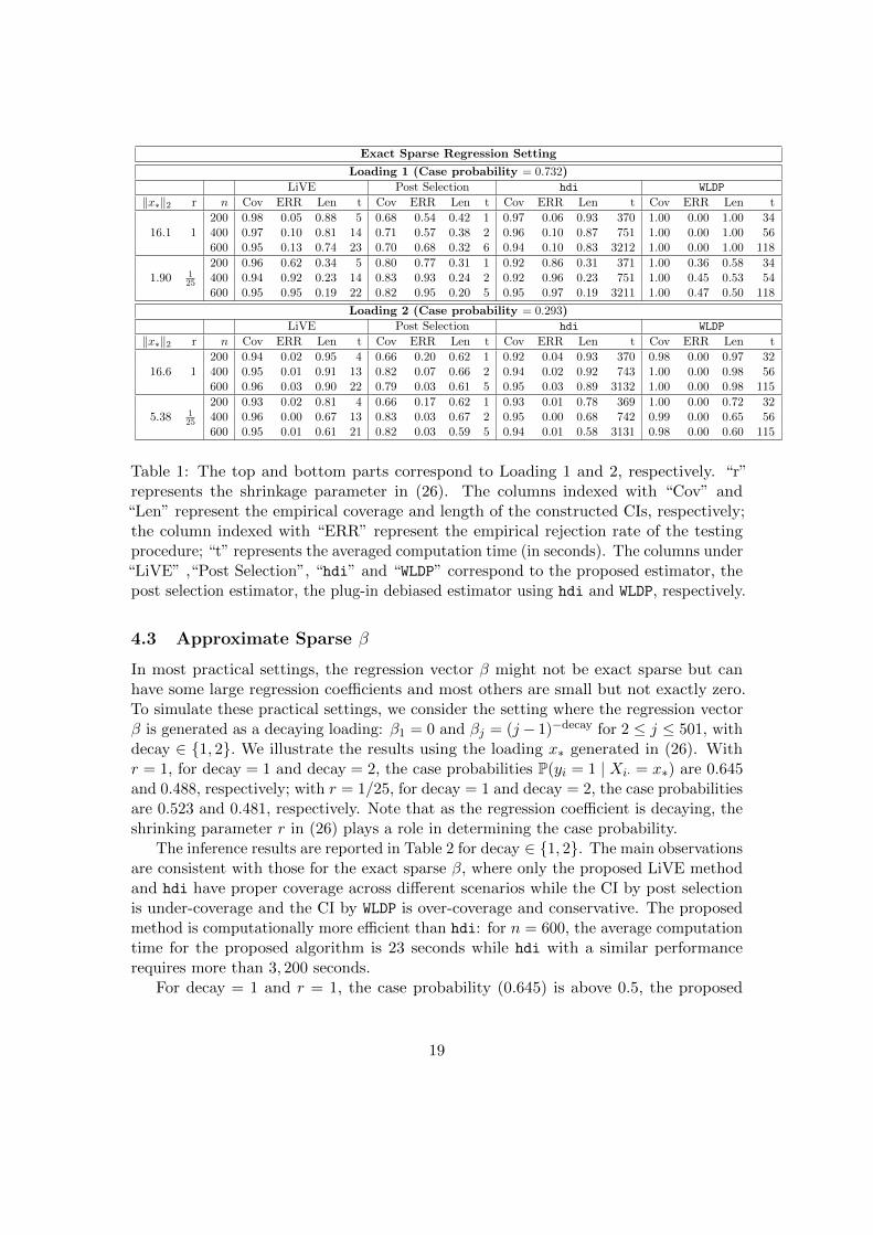
In Table 1, we compare the proposed LiVE method with post-selection, hdi andWLDP, in terms of CI construction and hypothesis testing. The coverage and lengths ofCIs are reported under the columns indexed with “Cov” and “Len”, respectively. TheCIs constructed by LiVE and hdi have coverage over different scenarios and the lengthsare reduced when a larger sample is used to construct the CI. WLDP suffers from the issueof over-coverage and the post-selection method suffers from under-coverage.

Regarding the testing procedure, we report the empirical rejection rate (ERR) of theproposed testing procedures, where ERR is defined as the proportion of null hypothesisin (2) being rejected out of the 500 replications. Under the null hypothesis, ERR isan empirical measure of the type I error; under the alternative hypothesis, ERR is anempirical measure of the power. For Loading 1 (alternative hypothesis), the empiricalpower increases with sample sizes, for all methods. For the case that ‖x∗‖2 is relativelysmall, the proposed LiVE method has a power above 0.90 when the sample size reaches400. For settings with large ‖x∗‖2, the power is not as high mainly due to the highvariance of the bias-corrected estimator. This is consistent with the theoretical resultsestablished in Proposition 3. On the contrary, even with sample size as large as 600 andrelatively small ‖x∗‖2, the test based on WLDP does not have a good power. For loading 2(null hypothesis), the proposed LiVE method, hdi and WLDP have type I error controlledacross all sample sizes while post selection does not have it controlled for the sample sizeat n = 200.

We have investigated the computational efficiency of all methods and reported theaveraged time of implementing each method under the column indexed with “t” (theunits are seconds). The proposed LiVE method is computationally efficient and canbe finished within 25 seconds on average. The hdi algorithm provides valid CIs butrequires around an hour to achieve the same goal for n = 600 and p = 501. The mainreason is that the hdi is not designed for inference for case probabilities and requires theimplementation of p high-dimensional penalization algorithm for bias-correction.

We report Root Mean Squared Error (RMSE), the bias and also the standard deviationof the proposed LiVE estimator, plug-in Lasso, post-selection, hdi and WLDP in Table3 in Section B.1 of the supplementary material. It is observed that the plug-in Lassoestimator cannot be used for confidence interval construction as its bias component is aslarge as its variance component and the uncertainty of the bias component is hard toquantify.

Post selection inference methods can produce incorrect inference due to the fact thatthe model selection uncertainty is not quantified. In the selection step, the post-selectionmethod can select either a larger model or a smaller model compared to the true one.As reported in Table 1, post selection is under-coverage since, in this specific simulationsetting, post-selection tends to select a relatively large set of variables and this resultsin perfect separation of cases and controls in the re-fitting step. In Section B.3 of thesupplementary material, we show another setting where the post-selection method selectsa smaller model and leads to a substantial omitted variable bias.

18

Exact Sparse Regression Setting

Loading 1 (Case probability = 0.732)

LiVE Post Selection hdi WLDP

‖x∗‖2 r n Cov ERR Len t Cov ERR Len t Cov ERR Len t Cov ERR Len t

16.1 1200 0.98 0.05 0.88 5 0.68 0.54 0.42 1 0.97 0.06 0.93 370 1.00 0.00 1.00 34400 0.97 0.10 0.81 14 0.71 0.57 0.38 2 0.96 0.10 0.87 751 1.00 0.00 1.00 56600 0.95 0.13 0.74 23 0.70 0.68 0.32 6 0.94 0.10 0.83 3212 1.00 0.00 1.00 118

1.90 125

200 0.96 0.62 0.34 5 0.80 0.77 0.31 1 0.92 0.86 0.31 371 1.00 0.36 0.58 34400 0.94 0.92 0.23 14 0.83 0.93 0.24 2 0.92 0.96 0.23 751 1.00 0.45 0.53 54600 0.95 0.95 0.19 22 0.82 0.95 0.20 5 0.95 0.97 0.19 3211 1.00 0.47 0.50 118

Loading 2 (Case probability = 0.293)

LiVE Post Selection hdi WLDP

‖x∗‖2 r n Cov ERR Len t Cov ERR Len t Cov ERR Len t Cov ERR Len t

16.6 1200 0.94 0.02 0.95 4 0.66 0.20 0.62 1 0.92 0.04 0.93 370 0.98 0.00 0.97 32400 0.95 0.01 0.91 13 0.82 0.07 0.66 2 0.94 0.02 0.92 743 1.00 0.00 0.98 56600 0.96 0.03 0.90 22 0.79 0.03 0.61 5 0.95 0.03 0.89 3132 1.00 0.00 0.98 115

5.38 125

200 0.93 0.02 0.81 4 0.66 0.17 0.62 1 0.93 0.01 0.78 369 1.00 0.00 0.72 32400 0.96 0.00 0.67 13 0.83 0.03 0.67 2 0.95 0.00 0.68 742 0.99 0.00 0.65 56600 0.95 0.01 0.61 21 0.82 0.03 0.59 5 0.94 0.01 0.58 3131 0.98 0.00 0.60 115

Table 1: The top and bottom parts correspond to Loading 1 and 2, respectively. “r”represents the shrinkage parameter in (26). The columns indexed with “Cov” and“Len” represent the empirical coverage and length of the constructed CIs, respectively;the column indexed with “ERR” represent the empirical rejection rate of the testingprocedure; “t” represents the averaged computation time (in seconds). The columns under“LiVE” ,“Post Selection”, “hdi” and “WLDP” correspond to the proposed estimator, thepost selection estimator, the plug-in debiased estimator using hdi and WLDP, respectively.

4.3 Approximate Sparse β

In most practical settings, the regression vector β might not be exact sparse but canhave some large regression coefficients and most others are small but not exactly zero.To simulate these practical settings, we consider the setting where the regression vectorβ is generated as a decaying loading: β1 = 0 and βj = (j− 1)−decay for 2 ≤ j ≤ 501, withdecay ∈ {1, 2}. We illustrate the results using the loading x∗ generated in (26). Withr = 1, for decay = 1 and decay = 2, the case probabilities P(yi = 1 | Xi· = x∗) are 0.645and 0.488, respectively; with r = 1/25, for decay = 1 and decay = 2, the case probabilitiesare 0.523 and 0.481, respectively. Note that as the regression coefficient is decaying, theshrinking parameter r in (26) plays a role in determining the case probability.

The inference results are reported in Table 2 for decay ∈ {1, 2}. The main observationsare consistent with those for the exact sparse β, where only the proposed LiVE methodand hdi have proper coverage across different scenarios while the CI by post selectionis under-coverage and the CI by WLDP is over-coverage and conservative. The proposedmethod is computationally more efficient than hdi: for n = 600, the average computationtime for the proposed algorithm is 23 seconds while hdi with a similar performancerequires more than 3, 200 seconds.

For decay = 1 and r = 1, the case probability (0.645) is above 0.5, the proposed

19

LiVE method and hdi achieve the correct coverage level but the testing procedureshave low powers. This matches with Proposition 3, that is, the power of the proposedtesting procedure tends to be low for the observation x∗ with very large ‖x∗‖2. Fordecay = 1 and r = 1/25, the case probability is 0.523 and this represents an alternativein the indistinguishable region and the power of the proposed testing procedure is low asexpected. For decay = 2, the testing procedures based on the proposed LiVE, hdi andWLDP have type I error controlled for both r = 1 and r = 1/25 while the post selectionmethod suffers from an inflated Type I error for the setting r = 1. The estimationresults are reported in Table 4 in Section B.2 of the supplementary material. The plug-inLasso estimator suffers from a large bias and cannot be used for confidence intervalconstruction.

The consistent performance of the proposed inference method suggests that the pro-posed method not only works for the exact sparse setting, but also for the approximatelysparse setting, which is simulated here to better approximate the practical data sets.

Approximate Sparse Regression Seting

decay = 1

LiVE Post Selection hdi WLDP

‖x∗‖2 r Prob n Cov ERR Len t Cov ERR Len t Cov ERR Len t Cov ERR Len t

16.1 1 0.645200 0.96 0.05 0.93 5 0.58 0.26 0.45 1 0.96 0.06 0.93 370 1.00 0.00 1.00 34400 0.96 0.04 0.85 14 0.60 0.31 0.41 2 0.97 0.07 0.90 751 1.00 0.00 1.00 56600 0.97 0.05 0.80 23 0.62 0.37 0.37 6 0.96 0.07 0.86 3212 1.00 0.00 1.00 118

1.09 125 0.523

200 0.96 0.06 0.40 5 0.69 0.13 0.31 1 0.96 0.05 0.39 371 1.00 0.00 0.75 34400 0.96 0.11 0.28 14 0.58 0.16 0.24 2 0.94 0.11 0.28 751 1.00 0.00 0.68 54600 0.97 0.07 0.24 22 0.71 0.09 0.21 5 0.96 0.04 0.24 3211 1.00 0.00 0.65 118

decay = 2

LiVE Post Selection hdi WLDP

‖x∗‖2 r Prob n Cov ERR Len t Cov ERR Len t Cov ERR Len t Cov ERR Len t

16.1 1 0.488200 0.95 0.04 0.91 5 0.66 0.14 0.37 1 0.94 0.03 0.92 370 1.00 0.00 1.00 34400 0.96 0.03 0.86 14 0.60 0.18 0.29 2 0.95 0.04 0.88 751 1.00 0.00 1.00 56600 0.96 0.03 0.78 23 0.67 0.15 0.27 6 0.93 0.03 0.85 3212 1.00 0.00 1.00 118

1.09 125 0.481

200 0.96 0.03 0.35 5 0.87 0.05 0.22 1 0.95 0.03 0.38 371 1.00 0.00 0.75 34400 0.93 0.04 0.27 14 0.83 0.06 0.15 2 0.93 0.03 0.27 751 1.00 0.00 0.68 54600 0.96 0.02 0.22 22 0.73 0.02 0.12 5 0.94 0.02 0.23 3211 1.00 0.00 0.65 118

Table 2: The top and bottom parts correspond to decay = 1 and decay = 2, respectively.“r” and“Prob” represent the shrinkage parameter in (26) and Case Probability respectively.The columns indexed with “Cov” and “Len” represent the empirical coverage and lengthof the constructed CIs; the column indexed with “ERR” represent the empirical rejectionrate of the testing procedure; “t” represents the averaged computation time (in seconds).The columns under “LiVE” ,“Post Selection”, “hdi” and “WLDP” correspond to theproposed estimator, the post selection estimator, the plug-in debiased estimator usinghdi and WLDP respectively.

20

5 Real Data Analysis

We applied the proposed methods to develop preliminary models for predicting threerelated disease conditions, hypertension, hypertension that appears to be resistant tostandard treatment (henceforth “R-hypertension”), and hypertension with unexplainedlow blood potassium (henceforth “LP-hypertension”). The data were extracted fromthe Penn Medicine clinical data repository, including demographics, laboratory results,medication prescriptions, vital signs, and encounter meta information. The analysiscohort consisted of 348 patients who were at least 18 years old, had at least 5 officevisits over at least three distinct years between 2007 and 2017, and at least 2 officevisits were at one of the 37 primary care practices. Patient charts were reviewed bya dedicated physician to determine each of the three outcome statuses, and unclearcases were secondarily reviewed by an additional expert clinician. The prevalence ofthe three outcome variables were 39.4%, 8.1%, and 4.6%, respectively. LongitudinalEHR variables, which had varied values over multiple observations, were summarizedby minimum, maximum, mean, median, standard deviation, and/or skewness, and thesesummary statistics were used as predictors after appropriate normalization. Highlyright-skewed variables were log-transformed. We included 198 predictors in the finalanalyses, after removing those with missing values.

In our analysis, we randomly sampled 30 patients as the test sample, then theirpredictor vectors were treated as x∗. A prediction model for each outcome variable wasdeveloped using the remaining 318 patients and then applied to the test sample to obtainbias-corrected estimates of the case probabilities using our method. The left and rightcolumns in Figure 1 present results on two independent test samples, where the threerows within each column correspond to the three outcome variables. In each panel, thex-axis represents the predicted probability generated by our method, and the y-axisrepresents the true outcome status (1 or 0). In all six panels, the predicted probabilitiesby the LiVE method for true cases tended to be high and for true controls tended to below. This illustrates that the LiVE estimator in (12) is predictive for the true outcomestatus.

Figure 2 presented confidence intervals constructed using our method for the caseprobabilities shown in the top two panels in the right column in Figure 1, correspondingto prediction of hypertension and resistant hypertension. The length of the constructedconfidence intervals appeared to vary since each patient in the test sample had differentobserved predictors x∗. This observation is consistent with the established theory inTheorem 1, which states that the length of confidence interval depends on ‖x∗‖2. Moreinterestingly, the constructed confidence intervals appeared to be informative of theoutcome statuses for the majority of the test patients. For hypertension, 80% of theconfidence intervals lied either above or below 50%; For R-hypertension, 83% of theconfidence intervals lie either above or below 50%.

We further divide the 30 randomly sampled observations into two subgroups by theirtrue status and then investigate the performance of constructed confidence intervalsfor the subgroup of observations being cases and the other subgroup of observations

21

0.0 0.2 0.4 0.6 0.8 1.0

0.0

0.4

0.8

hypertension Sample A

Projected Probabilities

Labe

ls

0.0 0.2 0.4 0.6 0.8 1.0

0.0

0.4

0.8

hypertension Sample B

Projected Probabilities

Labe

ls

0.0 0.2 0.4 0.6 0.8 1.0

0.0

0.4

0.8

R−hypertension Sample A

Projected Probabilities

Labe

ls

0.0 0.2 0.4 0.6 0.8 1.0

0.0

0.4

0.8

R−hypertension Sample B

Projected ProbabilitiesLa

bels

0.0 0.2 0.4 0.6 0.8 1.0

0.0

0.4

0.8

LP−hypertension Sample A

Projected Probabilities

Labe

ls

0.0 0.2 0.4 0.6 0.8 1.0

0.0

0.4

0.8

LP−hypertension Sample B

Projected Probabilities

Labe

ls

Figure 1: Performance for predicting three phenotypes in two random sub-samples.

being controls. On the left panel of Figure 2, the observations with indexes between1 and 11 correspond to cases (observations with hypertension) while the remaining 19observations correspond to observations without hypertension. Out of the 11 observationswith hypertension, six constructed CIs are predictive with the whole interval above 0.5,one is misleading as the interval is below 0.5 and the remaining four are not predictive asthe CIs come cross 0.5; Out of the 19 patients without hypertension, 17 constructed CIsare below 0.5 and hence predictive but the remaining two are not. On the right hand sideof Figure 2, the observations with indexes between 1 and 4 correspond to observationswith R-hypertension while the remaining 26 observations correspond to the observationswithout R-hypertension. Out of the four observations with R-hypertension, only oneconstructed CI is predictive and the other three are not; out of the 26 observations withoutR-hypertension, 24 are predictive and the other two are not. Overall, the constructedCIs are predictive for the outcome for 77% (hypertension), 83%(R-hypertension), and77% (LP-hypertension) of subjects, where a constructed CI is predictive if either theconstructed CI lies above 0.5 for the true case or below 0.5 for the true control. Thisdemonstrated the practical usefulness of the developed models for evaluating the outcomestatus of patients, the labor-intensive chart review may be avoided for the majority ofpatients.

22

0 5 10 15 20 25 30

0.0

0.4

0.8

hypertension Sample B

Index

Pro

ject

ed P

roba

bilit

ies

0 5 10 15 20 25 30

0.0

0.4

0.8

R−hypertension Sample B

Index

Pro

ject

ed P

roba

bilit

ies

Figure 2: Confidence interval construction: on the left panel, indexes 1 to 11 correspond toobservations with hypertension; indexes 12 to 30 correspond to those without hypertension.On the right panel, indexes 1 to 4 correspond to observations with R-hypertension; indexes5 to 30 correspond to those without R-hypertension.

The additional results corresponding to the remaining four panels are presented inFigure 3 in the supplementary materials. The observation is similar to that reported inFigure 2.

6 Proof

We provide the proof of Theorem 1 in Section 6.1 and that of Lemma 1 in Section 6.2.The remaining of the proof is postponed to Section A in the supplementary material.

We introduce the following events and also two lemmas to facilitate the proof.

A1 =

{max

1≤i≤n, 1≤j≤p|Xij | ≤ C

√log n+ log p

}, A2 =

{min

‖η‖2=1,‖ηSc‖1≤C‖ηS‖1

1

n

n∑i=1

(Xᵀi·η)

2 ≥ cλmin (Σ)

}

A3 =

{min

1≤i≤n

exp (Xᵀi·β)

[1 + exp (Xᵀi·β)]

2 ≥ c2min

}, A4 =

{λ0 =

∥∥∥∥∥ 1

n

n∑i=1

εiXi

∥∥∥∥∥∞

≤ C√

log p

n

}

A5 =

{‖β − β‖2 ≤ C

√k log p

n

}, A6 =

{‖(β − β)Sc‖1 ≤ C0‖(β − β)S‖1

}(28)

where S denotes the support of the high-dimensional vector β. The following lemma 2controls the probability of these defined events and the proof is omitted as it is similarto Lemma 4 in [9].

Lemma 2. Suppose Conditions (A1) and (A2) hold, then

P(∩4i=1Ai

)≥ 1− exp(−cn)− p−c (29)

23

and on the event ∩4i=1Ai, the events A5 and A6 hold.

The following Lemma is about the Taylor expansion of logit function and the corre-sponding proof is presented in Section A.4 in the supplementary material.

Lemma 3. For h(x) = exp(x)1+exp(x) , we have

(h′(B)

)−1(h(x)− h(B)) = (x− a) +

∫ 1

0(1− t)(x− a)2h

′′(a+ t(x− a))

h′(B)dt. (30)

where

h′(x) =exp(x)

(1 + exp(x))2and h′′(x) =

2 exp(2x)

(1 + exp(x))3

We further have

exp (− |x− a|) ≤ h′(x)

h′(B)≤ exp (|x− a|) and

∣∣∣∣ h′(x)

h′(B)− 1

∣∣∣∣ ≤ exp (|x− a|) (31)

and ∣∣∣∣∫ 1

0(1− t)(x− a)2h

′′(a+ t(x− a))

h′(B)dt

∣∣∣∣ ≤ exp(|x− a|)(x− a)2 (32)

6.1 Proof of Theorem 1

Proof of (18). We first note that, on the event A3,

uᵀ

[1

n2

n∑i=1

Xi·Xᵀi·

]u ≤ V ≤ 1

c2min

uᵀ

[1

n2

n∑i=1

Xi·Xᵀi·

]u. (33)

To control the upper bound part√

V ≤ C0‖x∗‖2n , we define the following events

B1 ={∥∥∥ΣΣ−1x∗ − x∗

∥∥∥∞≤ ‖x∗‖2λn

}B2 =

{∥∥∥xᵀ∗ΣΣ−1x∗ − ‖x∗‖22∣∣∣ ≤ ‖x∗‖22λn}

B3 ={‖XΣ−1x∗‖∞ ≤ ‖x∗‖2τn

} (34)

On the event ∩3i=1Bi, then u = Σ−1x∗ satisfies the constraints (9), (10) and (11). As a

consequence, the feasible set is non-empty on the event ∩3i=1Bi and we further obtain an

upper bound for the minimum value, that is,

V ≤ xᵀ∗Σ−1ΣΣ−1x∗/n. (35)

The following lemma controls the probability of the above events,

24

Lemma 4. Suppose Condition (A1) holds and λn �√

log pn and τn . nδ for 0 < δ < 1

2 ,

thenP(∩3i=1Bi

)≥ 1− n−c − p−c. (36)

The proof of the lower bound part√

V ≥ c0‖x∗‖2n is facilitated by the optimization

constraint (9). We define a proof-facilitating optimization problem,

u = arg minu∈Rp

uᵀ

(1

n

n∑i=1

Xi·Xᵀi·

)u

subject to |xᵀ∗Σu− ‖x∗‖22| ≤ ‖x∗‖22λn

(37)

Note that u satisfies the feasible set of (37) and hence

uᵀ

(1

n

n∑i=1

Xi·Xᵀi·

)u ≥ uᵀ

(1

n

n∑i=1

Xi·Xᵀi·

)u

≥ uᵀ(

1

n

n∑i=1

Xi·Xᵀi·

)u+ t

((1− λn)‖x∗‖22 − xᵀ∗Σu

)for any t ≥ 0,

(38)

where the last inequality follows from the constraint of (37). Note that for a given t ≥ 0,we have

uᵀ

(1

n

n∑i=1

Xi·Xᵀi·

)u+ t

((1− λn)‖x∗‖22 − xᵀ∗Σu

)≥ min

u∈Rpuᵀ

(1

n

n∑i=1

Xi·Xᵀi·

)u+ t

((1− λn)‖x∗‖22 − xᵀ∗Σu

).

(39)

By solving the minimization problem of the right hand side of (39), we have the minimizeru∗ satisfies Σu∗ = t

2 Σx∗ and hence the minimized value of the right hand side of (39) is

− t2

4xᵀ∗Σx∗ + t(1− λn)‖x∗‖22.

Combined with (38) and (39), we have

uᵀ

(1

n

n∑i=1

Xi·Xᵀi·

)u ≥ max

t≥0

[− t

2

4xᵀ∗Σx∗ + t(1− λn)‖x∗‖22

]. (40)

For t∗ = 2(1−λn)‖x∗‖22

xᵀ∗Σx∗> 0, the minimum of the right hand side of (40) is achieved and

hence establish

uᵀ

(1

n

n∑i=1

Xi·Xᵀi·

)u ≥ (1− λn)2‖x∗‖42

xᵀ∗Σx∗. (41)

Proof of (16). The limiting distribution in (16) follows from the decomposition (8), thevariance control in (18), Lemma 1 and Proposition 4 and the following lemma.

25

Lemma 5. Suppose that Conditions (A1) and (A2) hold and τn defined in (11) satisfies

(log n)1/2 . τn � n1/2, then

1

V 1/2uᵀ

1

n

n∑i=1

[h(Xᵀi·β)(1− h(Xᵀ

i·β))]−1Xi·εi → N(0, 1) (42)

where V is defined in (17).

6.2 Proof of Lemma 1

To start the proof, we recall that h(z) = exp(z)1+exp(z) and define the functions gi for 1 ≤ i ≤ n

gi(ti) =

( exp (Xᵀi·β + ti)

(1 + exp (Xᵀi·β + ti))

2

)−1

−

(exp (Xᵀ

i·β)

(1 + exp (Xᵀi·β))

2

)−1 uᵀXi·,

and the space for δ ∈ Rp as

C =

{δ : ‖δSc‖1 ≤ c‖δS‖1, ‖δ‖2 ≤ C∗

√k log p

n

}. (43)

for some positive constants c > 0 and C∗ > 0. We further define

T = {t = (t1, · · · , tn) : ti = Xᵀi·δ where δ ∈ C} , (44)

We can rewrite the main component of the left hand side of (24) as∣∣∣∣∣∣∣uᵀ1√n

n∑i=1

exp(Xᵀ

i·β)(1 + exp(Xᵀ

i·β))2

−1

−

(exp (Xᵀ

i·β)

(1 + exp (Xᵀi·β))

2

)−1Xi·εi

∣∣∣∣∣∣∣ · 1A1∩A3∩A5∩A6

≤ supδ∈C

∣∣∣∣∣ 1√n

n∑i=1

gi(Xᵀi·δ) · 1A1∩A3 · εi

∣∣∣∣∣ = supt∈T

∣∣∣∣∣ 1√n

n∑i=1

gi(ti) · 1A1∩A3 · εi

∣∣∣∣∣(45)

where C is defined in (43) and T is defined in (44). In the following, we control the lastpart of (45) via applying the symmetrization technique [38] stated in Lemma 6 and thecontraction principle in Lemma 7. The proofs of Lemma 6 and Lemma 7 are presentedin Sections A.5 and A.6 in the supplementary materials, respectively.

Lemma 6. Suppose that y′i is an independent copy of yi and ε′i is defined as y′i−E(y′i | Xi).For all convex nondecreasing functions Φ : R+ → R+, then

EΦ

(supt∈T

∣∣∣∣∣n∑i=1

gi(ti)εi

∣∣∣∣∣)≤ EΦ

(supt∈T

∣∣∣∣∣n∑i=1

gi(ti)ξi

∣∣∣∣∣), (46)

whereξi = εi − ε′i = yi − y′i.

26

The following lemma is a modification of Theorem 2.2 in [26], where the result in[26] was only developed for i.i.d Rademacher variables ξi. The following lemma is moregeneral in the sense that ξ1, ξ2, · · · , ξn are only required to be independent and satisfythe probability distribution (49).

Lemma 7. Let t = (t1, · · · , tn) ∈ T ⊂ Rn and let φi : R→ R, i = 1, · · · , n be functionssuch that φi(0) = 0 and

|φi(u)− φi(v)| ≤ |u− v|, u, v ∈ R. (47)

For all convex nondecreasing functions Φ : R+ → R+, then

EΦ

(1

2supt∈T

∣∣∣∣∣n∑i=1

φi(ti)ξi

∣∣∣∣∣)≤ EΦ

(supt∈T

∣∣∣∣∣n∑i=1

tiξi

∣∣∣∣∣), (48)

where {ξi}1≤i≤n are independent random variables with the probability density function

P (ξi = 1) = P (ξi = −1) ∈ [0,1

2], P (ξi = 0) = 1− 2P (ξi = 1) . (49)

We will apply Lemmas 6 and 7 and provide a sharp control for supt∈T

∣∣∣ 1√n

∑ni=1 gi(ti) · 1A1∩A3 · εi

∣∣∣in (45). For t, s ∈ T ⊂ Rn, then there exist δt, δs ∈ C ⊂ Rp such that

ti − si = Xᵀi·(δt − δs

)and ti = Xᵀ

i·δt for 1 ≤ i ≤ n.

Hence on the event A1,

max

{max

1≤i≤n|ti − si|, max

1≤i≤n|ti|}≤ Ck

√log p

n

√log p+ log n ≤ 1. (50)

where the last inequality follows as long as√n ≥ k log p

(1 +

√lognlog p

)Define q(x) =

(exp(x)

(1+exp(x))2

)−1and then

gi(si)− gi(ti) = (q (Xᵀi·β + si)− q (Xᵀ

i·β + ti)) uᵀXi·

=

(q (Xᵀ

i·β + si)

q (Xᵀi·β + ti)

− 1

)q (Xᵀ

i·β + ti)

q (Xᵀi·β)

q (Xᵀi·β) uᵀXi·

(51)

By (31), we have ∣∣∣∣q (Xᵀi·β + si)

q (Xᵀi·β + ti)

− 1

∣∣∣∣ ≤ |exp(|si − ti|)− 1| ≤ e|si − ti|, (52)

27

where the last inequality holds as long as |si − ti| is sufficiently small, as verified in (50).

Similarly, we establish thatq(Xᵀ

i·β+ti)q(Xᵀ

i·β)≤ e. Combined with (51) and (52), we obtain

|gi(si)− gi(ti)| ≤1

c2min

e2 |si − ti| |uᵀXi·| ≤1

c2min

e2 |si − ti| ‖x∗‖2τn, (53)

where the last inequality follows from the constraint (11). By applying (53), we have

1

Ln|gi(ti)− gi(si)| · 1A1∩A3 ≤ |ti − si| where Ln =

e2

c2min

‖x∗‖2τn. (54)

Define φi(ti) = 1Lngi(ti) · 1A1 . We then apply (46) and (48) with Φ(x) = x and obtain

Eξ|X supt∈T

∣∣∣∣∣ 1nn∑i=1

φi(ti) · 1A1∩A3ξi

∣∣∣∣∣ ≤ 2Eξ|X supδ∈C

∣∣∣∣∣ 1nn∑i=1

δᵀXi·ξi

∣∣∣∣∣and hence

E supt∈T

∣∣∣∣∣ 1nn∑i=1

φi(ti) · 1A1∩A3ξi

∣∣∣∣∣ ≤ 2E supδ∈C

∣∣∣∣∣ 1nn∑i=1

δᵀXi·ξi

∣∣∣∣∣ .Note that

E supδ∈C

∣∣∣∣∣ 1nn∑i=1

δᵀXi·ξi

∣∣∣∣∣ ≤ supδ∈C‖δ‖1E

∥∥∥∥∥ 1

n

n∑i=1

Xi·ξi

∥∥∥∥∥∞

≤ supδ∈C‖δ‖1

√2 log p

n‖Xi·‖ψ2 ,

where the last inequality follows from the fact that 1√n

∑ni=1Xi·ξi is sub-gaussian random

variable with sub-gaussian norm ‖Xi·‖ψ2 . Combined with the fact that supδ∈C ‖δ‖1 ≤Ck√

log pn , we establish E supδ∈C

∣∣ 1n

∑ni=1 δ

ᵀXi·ξi∣∣ ≤ C k log p

n ‖Xi·‖ψ2 and hence

E supt∈T

∣∣∣∣∣ 1nn∑i=1

φi(ti) · 1A1ξi

∣∣∣∣∣ ≤ Ck log p

n‖Xi·‖ψ2 .

By Chebyshev’s inequality, we have

P

(supt∈T

∣∣∣∣∣ 1nn∑i=1

gi(ti) · 1A1ξi

∣∣∣∣∣ ≥ Ct‖x∗‖2τnk log p

n‖Xi·‖ψ2

)≤ 1

t

By (45), we establish that (24) holds with probability larger than 1−(1t +p−c+exp(−cn)).

References

[1] Zakhriya Alhassan, David Budgen, Riyad Alshammari, and Noura Al Moubayed.Predicting current glycated hemoglobin levels in adults from electronic health records:Validation of multiple logistic regression algorithm. JMIR Medical Informatics, 2020.

28

[2] Susan Athey, Guido W Imbens, and Stefan Wager. Approximate residual balancing:debiased inference of average treatment effects in high dimensions. Journal of theRoyal Statistical Society: Series B (Statistical Methodology), 80(4):597–623, 2018.

[3] Francis Bach. Self-concordant analysis for logistic regression. Electronic Journal ofStatistics, 4:384–414, 2010.

[4] Heejung Bang and James M Robins. Doubly robust estimation in missing data andcausal inference models. Biometrics, 61(4):962–973, 2005.

[5] Alexandre Belloni and Victor Chernozhukov. Least squares after model selection inhigh-dimensional sparse models. Bernoulli, 19(2):521–547, 2013.

[6] Alexandre Belloni, Victor Chernozhukov, and Christian Hansen. High-dimensionalmethods and inference on structural and treatment effects. Journal of EconomicPerspectives, 28(2):29–50, 2014.

[7] Peter Buhlmann and Sara van de Geer. Statistics for high-dimensional data: methods,theory and applications. Springer Science & Business Media, 2011.

[8] Florentina Bunea. Honest variable selection in linear and logistic regression modelsvia `1 and `1+ `2 penalization. Electronic Journal of Statistics, 2:1153–1194, 2008.

[9] T. Tony Cai and Zijian Guo. Confidence intervals for high-dimensional linearregression: Minimax rates and adaptivity. The Annals of Statistics, 45(2):615–646,2017.

[10] Tianxi Cai, Tony Cai, and Zijian Guo. Optimal statistical inference for individualizedtreatment effects in high-dimensional models. Journal of the Royal Statistical Society:Series B (Statistical Methodology), 2019.

[11] Victor M Castro, Jessica Minnier, Shawn N Murphy, Isaac Kohane, Susanne EChurchill, Vivian Gainer, Tianxi Cai, Alison G Hoffnagle, Yael Dai, Stefanie Block,Sydney R Weill, Mireya Nadal-Vicens, Alisha R Pollastri, J Niels Rosenquist, SergeyGoryachev, Dost Ongur, Pamela Sklar, Roy H Perlis, Jordan W Smoller, andInternational Cohort Collection for Bipolar Disorder Consortium. Validation ofelectronic health record phenotyping of bipolar disorder cases and controls. TheAmerican Journal of Psychiatry, 172:363–372, 2015.

[12] Cristiana Catena, GianLuca Colussi, Roberta Lapenna, Elisa Nadalini, AlessandraChiuch, Pasquale Gianfagna, and Leonardo A. Sechi. Long-term cardiac effects ofadrenalectomy or mineralocorticoid antagonists in patients with primary aldostero-nism. Hypertension, 50:911–918, 2007.

[13] Victor Chernozhukov, Denis Chetverikov, Mert Demirer, Esther Duflo, ChristianHansen, Whitney Newey, and James Robins. Double/debiased machine learning fortreatment and structural parameters, 2018.

29

[14] Ruben Dezeure, Peter Buhlmann, Lukas Meier, and Nicolai Meinshausen. High-dimensional inference: Confidence intervals, p-values and r-software hdi. Statisticalscience, pages 533–558, 2015.

[15] Muhammad Faisal, Andy Scally, Robin Howes, Kevin Beatson, Donald Richardson,and Mohammed A Mohammed. A comparison of logistic regression models withalternative machine learning methods to predict the risk of in-hospital mortality inemergency medical admissions via external validation. Health Informatics Journal,26:34–44, 2020.

[16] Max H Farrell. Robust inference on average treatment effects with possibly morecovariates than observations. Journal of Econometrics, 189(1):1–23, 2015.

[17] John Fox. Applied regression analysis and generalized linear models. Sage Publica-tions, 2015.

[18] Jerome Friedman, Trevor Hastie, and Rob Tibshirani. Regularization paths forgeneralized linear models via coordinate descent. Journal of Statistical Software,2010.

[19] John W. Funder, Robert M. Carey, Franco Mantero, M. Hassan Murad, MartinReincke, Hirotaka Shibata, Michael Stowasser, and William F. Young Jr. Themanagement of primary aldosteronism: Case detection, diagnosis, and treatment:An endocrine society clinical practice guideline. The Journal of Clinical Endocrinology& Metabolism, 101:1889–1916, 2016.

[20] A Hannemann and H Wallaschofski. Prevalence of primary aldosteronism in patient’scohorts and in population-based studies–a review of the current literature. Hormoneand Metabolic Research, 44:157–162, 2011.

[21] Na Honga, Andrew Wena, Daniel J. Stonea, Shintaro Tsujia, Paul R. Kingsburya,Luke V. Rasmussenb, Jennifer A. Pachecob, Prakash Adekkanattuc, Fei Wangc,Yuan Luob, Jyotishman Pathakc, Hongfang Liua, and Guoqian Jiang. Developing afhir-based ehr phenotyping framework: A case study for identification of patientswith obesity and multiple comorbidities from discharge summaries. Journal ofBiomedical Informatics, 2019.

[22] Jian Huang and Cun-Hui Zhang. Estimation and selection via absolute penalizedconvex minimization and its multistage adaptive applications. Journal of MachineLearning Research, 13(Jun):1839–1864, 2012.

[23] Adel Javanmard and Andrea Montanari. Confidence intervals and hypothesistesting for high-dimensional regression. The Journal of Machine Learning Research,15(1):2869–2909, 2014.

[24] Joseph DY Kang and Joseph L Schafer. Demystifying double robustness: A com-parison of alternative strategies for estimating a population mean from incompletedata. Statistical science, 22(4):523–539, 2007.

30

[25] Sabine C Kayser, Tanja Dekkers, Hans J Groenewoud, Gert Jan van der Wilt,J Carel Bakx, Mark C van der Wel, Ad R Hermus, Jacques W Lenders, and JaapDeinum. Study heterogeneity and estimation of prevalence of primary aldostero-nism: A systematic review and meta-regression analysis. The Journal of ClinicalEndocrinology & Metabolism, 101:2826–2835, 2016.

[26] Vladimir Koltchinskii. Oracle Inequalities in Empirical Risk Minimization andSparse Recovery Problems: Ecole d?Ete de Probabilites de Saint-Flour XXXVIII-2008, volume 2033. Springer Science & Business Media, 2011.

[27] Yen-Hung Lin, Lian-Yu Lin, Aaron Chen, Xue-Ming Wu, Jen-Kuang Lee, Ta-ChenSu, Vin-Cent Wu, Shih-Chieh Chueh, Wei-Chou Lin, Men-Tzung Lo, Pa-ChunWang, Yi-Lwun Ho, Kwan-Dun Wu, and TAIPAI Study Group. Adrenalectomyimproves increased carotid intima-media thickness and arterial stiffness in patientswith aldosterone producing adenoma. Atherosclerosis, 221:154–159, 2012.

[28] Rong Ma, T Tony Cai, and Hongzhe Li. Global and simultaneous hypothesis testingfor high-dimensional logistic regression models. arXiv preprint arXiv:1805.06970,2018.

[29] Lukas Meier, Sara Van De Geer, and Peter Buhlmann. The group lasso for logisticregression. Journal of the Royal Statistical Society: Series B (Statistical Methodology),70(1):53–71, 2008.

[30] Sahand Negahban, Bin Yu, Martin J Wainwright, and Pradeep K Ravikumar. Aunified framework for high-dimensional analysis of m-estimators with decomposableregularizers. In Advances in Neural Information Processing Systems, pages 1348–1356,2009.

[31] Yang Ning and Han Liu. A general theory of hypothesis tests and confidence regionsfor sparse high dimensional models. The Annals of Statistics, 45(1):158–195, 2017.

[32] Ravi B. Parikh, Christopher Manz, Corey Chivers, Susan Harkness Regli, JenniferBraun, Michael E. Draugelis, Lynn M. Schuchter, Lawrence N. Shulman, Amol S.Navathe, Mitesh S. Pate, and Nina R. OConnor. Machine learning approaches topredict 6-month mortality among patients with cancer. JAMA Network Open, 2019.

[33] Judea Pearl. Causality: models, reasoning and inference, volume 29. Springer, 2000.

[34] Martin Reincke, Evelyn Fischer, Sabine Gerum, Katrin Merkle, Sebastian Schulz,Anna Pallauf, Marcus Quinkler, Gregor Hanslik, Katharina Lang, Stefanie Hah-ner, Bruno Allolio, Christa Meisinger, Rolf Holle, Felix Beuschlein, MartinBidlingmaier, Stephan Endres, and German Conn’s Registry-Else Krner-Fresenius-Hyperaldosteronism Registry. Observational study mortality in treated primaryaldosteronism: the german conn’s registry. Hypertension, 60:618–624, 2012.

[35] Paul R Rosenbaum and Donald B Rubin. The central role of the propensity scorein observational studies for causal effects. Biometrika, 70(1):41–55, 1983.

31

[36] Pragya Sur and Emmanuel J Candes. A modern maximum-likelihood theory forhigh-dimensional logistic regression. Proceedings of the National Academy of Sciences,116(29):14516–14525, 2019.

[37] Pragya Sur, Yuxin Chen, and Emmanuel J Candes. The likelihood ratio test in high-dimensional logistic regression is asymptotically a rescaled chi-square. Probabilitytheory and related fields, 175(1-2):487–558, 2019.

[38] Sara van de Geer. Empirical Processes in M-estimation. Cambridge UP, 2006.

[39] Sara van de Geer, Peter Buhlmann, Yaacov Ritov, and Ruben Dezeure. On asymp-totically optimal confidence regions and tests for high-dimensional models. TheAnnals of Statistics, 42(3):1166–1202, 2014.

[40] Cun-Hui Zhang and Stephanie S Zhang. Confidence intervals for low dimensionalparameters in high dimensional linear models. Journal of the Royal StatisticalSociety: Series B (Statistical Methodology), 76(1):217–242, 2014.

[41] Yinchu Zhu and Jelena Bradic. Linear hypothesis testing in dense high-dimensionallinear models. Journal of the American Statistical Association, 113(524):1583–1600,2018.

32

A Additional Proofs

A.1 Proof of Proposition 4

Proof of (20) The first inequality of (20) follows from Holder’s inequality and the secondinequality follows from Condition (B).Proof of (21) By Cauchy inequality, we have

√n

∣∣∣∣∣uᵀ 1

n

n∑i=1

Xi·∆i

∣∣∣∣∣ ≤ max1≤i≤n

|uᵀXi·|1√n

n∑i=1

|∆i| ≤ τn‖x∗‖21√n

n∑i=1

|∆i| (55)

By Lemma 3, we have |∆i| ≤ exp(|Xᵀ

i·(β − β)|)(

Xᵀi·(β − β)

)2. On the event A =

∩6i=1Ai, we have

n∑i=1

|∆i| ≤n∑i=1

exp(|Xᵀ

i·(β − β)|)(

Xᵀi·(β − β)

)2

≤ exp(

max |Xij | · ‖β − β‖1) n∑i=1

(Xᵀi·(β − β)

)2≤ C

n∑i=1

(Xᵀi·(β − β)

)2.

(56)

where the second inequality follows from Holder inequality and the last inequality follows

from the fact that√n� k log p

(1 +

√lognlog p

). On the event A, we have

1

n

n∑i=1

(Xᵀi·(β − β)

)2≤ C‖β − β‖22 ≤ C

k log p

n. (57)

Together with (55) and (56), we establish that, on the event A,

√n

∣∣∣∣∣uᵀ 1

n

n∑i=1

Xi·∆i

∣∣∣∣∣ ≤ Cτn‖x∗‖2k log p√n

. (58)

A.2 Proof of Lemma 5

1

n

n∑i=1

(exp (Xᵀ

i·β)

(1 + exp (Xᵀi·β))

2

)−1

uᵀXi·εi → N(0,V) (59)

Define

Wi =1√V

(exp (Xᵀ

i·β)

(1 + exp (Xᵀi·β))

2

)−1

uᵀXi·εi (60)

33

Conditioning on X, then {Wi}1≤i≤n are independent random variables with E(Wi |Xi) = 0 and

∑ni=1 Var(Wi | Xi) = n2. To establish (59), it is sufficient to check the

Lindeberg’s condition, that is, for any constant ε > 0,

limn→∞

1

n2

n∑i=1

E(W 2i 1{|Wi|≥ε

√n})

= 0. (61)

Note that

max1≤i≤n

∣∣∣∣∣∣ 1√V

(exp (Xᵀ

i·β)

(1 + exp (Xᵀi·β))

2

)−1

uᵀXi·εi

∣∣∣∣∣∣ ≤ 2max1≤i≤n |uᵀXi·|√

V≤ 2τn‖x∗‖2√

V≤ ε√n

(62)

where the first inequality follows from the fact that

(exp(Xᵀ

i·β)(1+exp(Xᵀ

i·β))2

)−1

εi ≤ 2cmin

, the

second inequality follows from |uᵀXi·| ≤ τn‖x∗‖2 and the last inequality follows from (18)and the condition τn �

√n. Then (61) follows from (62) and by Lindeberg’s central

limit theorem, we establish (59).

A.3 Proof of Proposition 1

For t ∈ (0, 1), by the definition of β, we have

`(β)+λ‖β‖1 ≤ `(β+t(β− β))+λ‖β+t(β− β)‖1 ≤ `(β+t(β−β))+(1−t)λ‖β‖1 +tλ‖β‖1(63)

where `(β) = 1n

∑ni=1 (log (1 + exp (Xᵀ

i·β))− yi · (Xᵀi·β)) . Then we have

`(β)− `(β + t(β − β))

t+ λ‖β‖1 ≤ λ‖β‖1 for any t ∈ (0, 1) (64)

and taking the limit t→ 0, we have

1

n

n∑i=1

(exp(Xᵀ

i·β)

1 + exp(Xᵀi·β)− yi

)Xᵀi·(β − β) + λ‖β‖1 ≤ λ‖β‖1 (65)

Note that(exp(Xᵀ

i·β)

1 + exp(Xᵀi·β)− yi

)Xᵀi·(β − β) =

(−εi +

(exp(Xᵀ

i·β)

1 + exp(Xᵀi·β)−

exp (Xᵀi·β)

1 + exp (Xᵀi·β)

))Xᵀi·(β − β)

= −εiXᵀi·(β − β) +

∫ 1

0

exp(Xᵀi·β + tXᵀ

i·(β − β))

[1 + exp

(Xᵀi·β + tXᵀ

i·(β − β))]2

(Xᵀi·(β − β)

)2dt

(66)

34

By (31), we have

exp(Xᵀi·β + tXᵀ

i·(β − β))

[1 + exp

(Xᵀi·β + tXᵀ

i·(β − β))]2 ≥

exp (Xᵀi·β)

[1 + exp (Xᵀi·β)]

2 exp(−t∣∣∣Xᵀ

i·(β − β)∣∣∣)

≥exp (Xᵀ

i·β)

[1 + exp (Xᵀi·β)]

2 exp

(−t max

1≤i≤n

∣∣∣Xᵀi·(β − β)

∣∣∣)(67)

Combined with (66), we have

∫ 1

0

exp(Xᵀi·β + tXᵀ

i·(β − β))

[1 + exp

(Xᵀi·β + tXᵀ

i·(β − β))]2

(Xᵀi·(β − β)

)2dt

≥exp (Xᵀ

i·β)

[1 + exp (Xᵀi·β)]

2

(Xᵀi·(β − β)

)2∫ 1

0exp

(−t max

1≤i≤n

∣∣∣Xᵀi·(β − β)

∣∣∣) dt=

exp (Xᵀi·β)

[1 + exp (Xᵀi·β)]

2

(Xᵀi·(β − β)

)2 1− exp(−max1≤i≤n

∣∣∣Xᵀi·(β − β)

∣∣∣)max1≤i≤n

∣∣∣Xᵀi·(β − β)

∣∣∣

(68)

Together with (65), we have

1− exp(−max1≤i≤n

∣∣∣Xᵀi·(β − β)

∣∣∣)max1≤i≤n

∣∣∣Xᵀi·(β − β)

∣∣∣(

1

n

n∑i=1

exp (Xᵀi·β)

[1 + exp (Xᵀi·β)]

2

(Xᵀi·(β − β)

)2)

+ λ‖β‖1

≤ λ‖β‖1 +1

n

n∑i=1

εiXᵀi·(β − β) ≤ λ‖β‖1 + λ0‖β − β‖1.

(69)By the fact that ‖β‖1 = ‖βS‖1 + ‖βSc − βSc‖1 and ‖β‖1 − ‖βS‖1 ≤ ‖βS − βS‖1, then wehave

1− exp(−max1≤i≤n

∣∣∣Xᵀi·(β − β)

∣∣∣)max1≤i≤n

∣∣∣Xᵀi·(β − β)

∣∣∣(

1

n

n∑i=1

exp (Xᵀi·β)

[1 + exp (Xᵀi·β)]

2

(Xᵀi·(β − β)

)2)

+ δ0λ0‖βSc − βSc‖1 ≤ (2 + δ0)λ0‖βS − βS‖1

(70)

Then we deduce (15) and

1− exp(−max1≤i≤n

∣∣∣Xᵀi·(β − β)

∣∣∣)max1≤i≤n

∣∣∣Xᵀi·(β − β)

∣∣∣(

1

n

n∑i=1

exp (Xᵀi·β)

[1 + exp (Xᵀi·β)]

2

(Xᵀi·(β − β)

)2)

≤ (2 + δ0)λ0‖βS − βS‖1.

(71)

35

Lemma 8. On the event A2 ∩ A3, then

1

n

n∑i=1

exp (Xᵀi·β)

[1 + exp (Xᵀi·β)]

2

(Xᵀi·(β − β)

)2≥ cλmin (Σ) ‖β − β‖22 (72)

Then (71) is further simplified as

1− exp(−max1≤i≤n

∣∣∣Xᵀi·(β − β)

∣∣∣)max1≤i≤n

∣∣∣Xᵀi·(β − β)

∣∣∣ cλmin (Σ) ‖β − β‖22 ≤ (2 + δ0)λ0‖βS − βS‖1 (73)

Case 1: Assume that

max1≤i≤n

∣∣∣Xᵀi·(β − β)

∣∣∣ ≤ c1 for some c1 > 0 (74)

then we have

1− exp(−max1≤i≤n

∣∣∣Xᵀi·(β − β)

∣∣∣)max1≤i≤n

∣∣∣Xᵀi·(β − β)

∣∣∣ =

∫ 1

0exp

(−t max

1≤i≤n

∣∣∣Xᵀi·(β − β)

∣∣∣) dt≥∫ 1

0exp (−tc1) dt =

1− exp (−c1)

c1

(75)

Define c2 = cλmin(Σ)2+δ0

1−exp(−c1)c1

, then we have

c2‖β − β‖22 ≤ λ0‖βS − βS‖1 ≤√kλ0‖βS − βS‖2 (76)

and hence

‖β − β‖2 .1

λmin

√kλ0 and ‖β − β‖1 ≤ kλ0 (77)

Case 2: Assume that (74) does not hold, then

1− exp(−max1≤i≤n

∣∣∣Xᵀi·(β − β)

∣∣∣)max1≤i≤n

∣∣∣Xᵀi·(β − β)

∣∣∣ ≥ 1− exp(−c1)

max1≤i≤n

∣∣∣Xᵀi·(β − β)

∣∣∣ (78)

Together with (73), we have

c2c1‖β − β‖22 ≤ λ0‖βS − βS‖1 max1≤i≤n

∣∣∣Xᵀi·(β − β)

∣∣∣ (79)

By max1≤i≤n

∣∣∣Xᵀi·(β − β)

∣∣∣ ≤ max |Xij | ‖β − β‖1 and (15), we further have

λ0‖βS − βS‖1 max1≤i≤n

∣∣∣Xᵀi·(β − β)

∣∣∣ ≤ 2 + 2δ0

δ0max |Xij |λ0‖βS − βS‖21

≤ 2 + 2δ0

δ0max |Xij | kλ0‖βS − βS‖22,

(80)

36

where the last inequality follows from Cauchy inequality. Combining (79) and (80), wehave shown that if (74) does not hold, then

max |Xij |2 + 2δ0

δ0kλ0 ≥ c2c1, (81)

Since this contradicts the assumption that max |Xij | kλ0 <c2c1δ02+2δ0

, we establish (77) andhence (15).

A.4 Proof of Lemma 3

We first introduce the following version of Taylor expansion.

Lemma 9. If f ′′(x) is continuous on an open interval I that contains a, and x ∈ I ,then

f(x)− f(a) = f ′(a)(x− a) +

∫ 1

0(1− t)(x− a)2f ′′(a+ t(x− a))dt (82)

By applying Lemma 9, we have

h(x)− h(a) = h′(a)(x− a) +

∫ 1

0(1− t)(x− a)2h′′(a+ t(x− a))dt

Divide both sides by (h′(a))−1, we establish (30). The inequality (31) follows from

h′(x)

h′(a)= exp(x− a)

[1 + exp(a)]2

[1 + exp(x)]2≤ exp(x− a) exp(2(a− x)+) = exp(|x− a|)

andh′(a)

h′(x)≤ exp(|x− a|)

The control of (32) follows from the following inequality,

h′′(a+ t(x− a))

h′(a)=

2 exp(2a+ 2t(x− a))

(1 + exp(a+ t(x− a)))3· (1 + exp(a))2

exp(a)

≤ 2 exp(t(x− a)) · (1 + exp(a))2

(1 + exp(a+ t(x− a)))2≤ 2 exp(t|x− a|)

A.5 Proof of Lemma 6

We start with the conditional expectation Ey|XΦ (supt∈T |∑n

i=1 gi(ti)εi|) and note that

Ey|XΦ

(supt∈T

∣∣∣∣∣n∑i=1

gi(ti)εi

∣∣∣∣∣)

= Ey|XΦ

(supt∈T

∣∣∣∣∣n∑i=1

gi(ti)εi −Ey′|X

n∑i=1

gi(ti)ε′i

∣∣∣∣∣).

37

Since supt∈T∣∣∑n

i=1 gi(ti)εi −Ey′|X∑n

i=1 gi(ti)ε′i

∣∣ ≤ Ey′|X supt∈T |∑n

i=1 gi(ti)(εi − ε′i)| andΦ is a non-decreasing function, we have

Φ

(supt∈T

∣∣∣∣∣n∑i=1

gi(ti)εi −Ey′|X

n∑i=1

gi(ti)ε′i

∣∣∣∣∣)≤ Φ

(Ey′|X sup

t∈T

∣∣∣∣∣n∑i=1

gi(ti)(εi − ε′i)

∣∣∣∣∣).

Since Φ is a convex function, we have

Ey|XΦ

(Ey′|X sup

t∈T

∣∣∣∣∣n∑i=1

gi(ti)(εi − ε′i)

∣∣∣∣∣)≤ E(y,y′)|XΦ

(supt∈T

∣∣∣∣∣n∑i=1

gi(ti)(εi − ε′i)

∣∣∣∣∣).

Integration of both sides of the above inequality leads to (46).

A.6 Proof of Lemma 7

The proof follows from that of Theorem 2.2 in [26] and some modification is necessary toextend the results to the general random variables ξ1, ξ2, · · · , ξn which are independentand follow the probability distribution (49).

We start with proving the following inequality for a function A : T → R,

EΦ

(supt∈T

[A(t) +

n∑i=1

φi(ti)ξi]

)≤ EΦ

(supt∈T

[A(t) +

n∑i=1

tiξi]

), (83)

We first prove the special case n = 1, which is reduced to be the following inequality,

EΦ

(supt∈T

[t1 + φ(t2)ξ0]

)≤ EΦ

(supt∈T

[t1 + t2ξ0]

), (84)

where T ⊂ R2 and P(ξ0 = 1) = P(ξ0 = −1) ∈ [0, 12 ] and P(ξ0 = 0) = 1 − 2P(ξ = 1). It

suffices to verify (84) by establishing the following inequality,

P(ξ0 = 1)Φ

(supt∈T

[t1 + φ(t2)]

)+ P(ξ0 = −1)Φ

(supt∈T

[t1 − φ(t2)]

)+ P(ξ0 = 0)Φ

(supt∈T

[t1]

)≤ P(ξ0 = 1)Φ

(supt∈T

[t1 + t2]

)+ P(ξ0 = −1)Φ

(supt∈T

[t1 − t2]

)+ P(ξ0 = 0)Φ

(supt∈T

[t1]

)This is equivalent to show

Φ

(supt∈T

[t1 + φ(t2)]

)+ Φ

(supt∈T

[t1 − φ(t2)]

)≤ Φ

(supt∈T

[t1 + t2]

)+ Φ

(supt∈T

[t1 − t2]

)(85)

The above inequality follows from the same line of proof as that in [26]. It remains to

38

prove the lemma by applying induction and (84), that is,

E(ξ1,··· ,ξn)|XΦ

(supt∈T

[A(t) +n∑i=1

φi(ti)ξi]

)= E(ξ1,··· ,ξn−1)|XEξn|XΦ

(supt∈T

[A(t) +n∑i=1

φi(ti)ξi]

)

≤ E(ξ1,··· ,ξn−1)|XEξn|XΦ

(supt∈T

[A(t) +n−1∑i=1

φi(ti)ξi + tnξn]

)

= Eξn|XE(ξ1,··· ,ξn−1)|XΦ

(supt∈T

[A(t) +

n−1∑i=1

φi(ti)ξi + tnξn]

)

Continuing the above equation, we establish E(ξ1,··· ,ξn)|XΦ (supt∈T [A(t) +∑n

i=1 φi(ti)ξi]) ≤E(ξ1,··· ,ξn)|XΦ (supt∈T [A(t) +

∑ni=1 tiξi]). Integration with respect to X leads to (83). In

the following, we will apply (83) to establish (48). Note that

EΦ

(1

2supt∈T

∣∣∣∣∣n∑i=1

φi(ti)ξi

∣∣∣∣∣)

= EΦ

1

2

(supt∈T

n∑i=1

φi(ti)ξi

)+

+1

2

(supt∈T

n∑i=1

φi(ti)(−ξi)

)+

≤ 1

2

EΦ

(supt∈T

n∑i=1

φi(ti)ξi

)+

+ EΦ

(supt∈T

n∑i=1

φi(ti)(−ξi)

)+

By applying (83) to the function u → Φ(u+), which is convex and non-decreasing, we

have EΦ(

(supt∈T∑n

i=1 φi(ti)ξi)+

)≤ EΦ (supt∈T

∑ni=1 tiξi) ≤ EΦ (supt∈T |

∑ni=1 tiξi|).

Then we establish (48).

B Additional Simulation Study

B.1 Exact Sparse

We consider the exact sparse regression setup (4.2) and report the results on estimationaccuracy in the following. In Table 3, we compare the proposed estimator, the postselection estimator, the plug-in hdi and WLDP and Lasso estimator in terms of Root MeanSquared Error (RMSE), bias and standard error. Through comparing the proposed andplug-in Lasso estimators, we observe that the bias component is reduced at the expenseof increasing the variance. Although the bias component is reduced, the total RMSE isnot necessarily decreasing after correcting the bias, since the increased variance can leadto a larger RMSE in total. The increase in variance is proportional to the loading norm‖x∗‖2; specifically, if the loading norm is large, we may suffer from a larger total RMSEafter bias-correction; if the loading norm is relatively small, the variance only increasesslightly and the total RMSE decreases due to the reduction of the bias; see loading 1with r = 1/25. This matches with the theoretical results presented in Theorem 1.

39

Exact Sparse Regression Setting

Loading 1 (Case probability = 0.732)

LiVE Post Selection hdi WLDP Lasso

‖x∗‖2 r n RMSE Bias SE RMSE Bias SE RMSE Bias SE RMSE Bias SE RMSE Bias SE

16.1 1200 0.33 -0.10 0.32 0.26 -0.02 0.26 0.38 -0.11 0.37 0.37 -0.04 0.37 0.14 -0.11 0.09400 0.26 -0.04 0.26 0.21 -0.02 0.21 0.31 -0.06 0.31 0.31 0.01 0.31 0.11 -0.08 0.07600 0.24 -0.05 0.24 0.20 -0.02 0.20 0.30 -0.08 0.29 0.30 -0.03 0.30 0.08 -0.06 0.06

1.09 125

200 0.10 -0.03 0.09 0.14 0.04 0.14 0.07 0.02 0.07 0.11 0.10 0.06 0.13 -0.11 0.07400 0.07 -0.02 0.07 0.09 0.03 0.09 0.06 0.02 0.06 0.09 0.08 0.05 0.10 -0.08 0.06600 0.06 -0.02 0.06 0.07 0.02 0.07 0.05 0.01 0.05 0.08 0.07 0.04 0.08 -0.06 0.05

Loading 2 (Case probability = 0.293)

LiVE Post Selection hdi WLDP Lasso

‖x∗‖2 r n RMSE Bias SE RMSE Bias SE RMSE Bias SE RMSE Bias SE RMSE Bias SE

16.6 1200 0.45 0.16 0.42 0.43 0.19 0.40 0.44 0.17 0.40 0.35 0.12 0.32 0.29 0.20 0.22400 0.38 0.10 0.37 0.33 0.08 0.32 0.39 0.10 0.37 0.29 0.08 0.28 0.23 0.13 0.19600 0.36 0.04 0.35 0.25 0.03 0.25 0.34 0.05 0.34 0.22 0.01 0.22 0.22 0.13 0.19

5.38 125

200 0.29 0.05 0.29 0.39 0.14 0.37 0.28 0.07 0.27 0.22 -0.02 0.22 0.27 0.17 0.21400 0.21 0.01 0.21 0.30 0.06 0.29 0.21 0.03 0.21 0.20 -0.03 0.20 0.22 0.13 0.18600 0.22 0.03 0.22 0.24 0.01 0.24 0.20 0.03 0.20 0.17 0.01 0.17 0.21 0.11 0.18

Table 3: The top and bottom parts correspond to Loading 1 and 2, respectively. “r”represents the shrinkage parameter in (26). The columns indexed with “RMSE”, “Bias”and “SE” represent the RMSE, bias and standard error, respectively. The columnsunder “LiVE”, “Post Selection”, “hdi”, “WLDP” and “Lasso” correspond to the proposedestimator, the post model selection estimator, the plug-in hdi, the plug-in WLDP and theplug-in Lasso estimator respectively.

B.2 Approximate Sparse

We report the estimation accuracy results in the approximate sparse regression setup (4.3)with decay ∈ {1, 2}. Table 4 summarizes the estimation accuracy results for Loading 1and the results are similar to the exact sparse setting in Table 3. Table 4 shows againthe plug-in Lasso estimator cannot be used for confidence interval construction owing toits large bias.

B.3 Comparison of Proposed Method with Post Selection Method

We now consider a challenging setting for post-selection and compare the post-selectionmethod with the proposed LiVE method. We set the values for the 500 regressioncoefficients as

βj =

(j − 1)/20 for 2 ≤ j ≤ 11 ; j 6= 9, 10

0.01 for j = 9, 10

0 for 12 ≤ j ≤ 501

We set the intercept β1 to be 0. The loading x∗ is generated as follows :Loading 3: We set xbasis,1 = 1 and generate xbasis,−1 ∈ R500 following N(0,Σ) with

40

Approximate Sparse Regression Setting

decay = 1

LiVE Post Selection hdi WLDP Lasso

‖x∗‖2 r Prob n RMSE Bias SE RMSE Bias SE RMSE Bias SE RMSE Bias SE RMSE Bias SE

16.1 1 0.645200 0.37 -0.03 0.37 0.31 -0.09 0.31 0.38 -0.04 0.38 0.38 -0.02 0.38 0.18 -0.14 0.11400 0.29 -0.05 0.28 0.28 -0.10 0.27 0.32 -0.06 0.31 0.32 0.02 0.32 0.16 -0.13 0.09600 0.24 -0.03 0.24 0.23 -0.05 0.23 0.28 -0.02 0.28 0.29 0.07 0.29 0.15 -0.13 0.08

1.09 125 0.523

200 0.10 -0.01 0.10 0.18 -0.03 0.18 0.10 0.02 0.10 0.12 0.05 0.11 0.07 -0.03 0.06400 0.08 -0.01 0.08 0.13 -0.01 0.13 0.08 0.01 0.08 0.09 0.04 0.09 0.05 -0.03 0.04600 0.06 -0.02 0.06 0.09 -0.03 0.08 0.05 0.01 0.05 0.05 0.05 0.05 0.05 -0.03 0.04

decay = 2

LiVE Post Selection hdi WLDP Lasso

‖x∗‖2 r Prob n RMSE Bias SE RMSE Bias SE RMSE Bias SE RMSE Bias SE RMSE Bias SE

16.1 1 0.488200 0.36 0.02 0.36 0.25 -0.02 0.25 0.38 0.01 0.38 0.41 0.02 0.41 0.08 0.00 0.08400 0.31 0.01 0.31 0.19 -0.01 0.19 0.32 -0.01 0.32 0.38 0.00 0.38 0.06 0.00 0.06600 0.26 -0.03 0.26 0.15 0.00 0.15 0.32 -0.02 0.32 0.26 -0.03 0.26 0.04 0.00 0.04

1.09 125 0.481

200 0.09 0.01 0.09 0.10 -0.01 0.10 0.10 0.01 0.10 0.11 0.01 0.11 0.04 0.01 0.04400 0.07 0.01 0.07 0.05 0.00 0.05 0.08 -0.01 0.08 0.09 -0.01 0.09 0.03 0.01 0.03600 0.06 0.01 0.06 0.05 -0.02 0.05 0.06 -0.01 0.06 0.06 -0.01 0.06 0.03 0.01 0.03

Table 4: The top and bottom parts correspond to decay = 1 and decay = 2, respectively.“r”and “Prob” represent the shrinkage parameter in (26) and case probability respectively.The columns indexed with “RMSE”, “Bias” and “SE” represent the RMSE, bias andstandard error, respectively. The columns under “LiVE”, “Post Selection”, “hdi”, “WLDP”and “Lasso” correspond to the proposed estimator, the post model selection estimator,the plug-in hdi, the plug-in WLDP and the Plug-in Lasso estimator respectively.

Σ = {0.51+|j−l|}1≤j,l≤500 and generate x∗ as

x∗,j =

xbasis,j for 1 ≤ j ≤ 11 ; j 6= 9, 10

10 for j = 9, 10125 · xbasis,j for 12 ≤ j ≤ 501

We construct the new β and x∗ as we believe this is a challenging setting for post selection.The insignificant regression coefficients β9, β10 make the corresponding covariates X·,9and X·,10 unlikely to be selected by Lasso in the first step. However, with enlarged entriesx∗,9, x∗,10, the corresponding covariates comprises a major part of the magnitude of thecase probability h(xᵀ∗β), thereby leading to a large omitted variable bias when theserelevant covariates are not selected by Lasso. We have observed in Table 5 that the postselection estimator has a large omitted variable bias and also produces a under-coveredconfidence interval.

B.4 Exact sparse with intercept

To explore the performance of the inference procedures in presence of an intercept, weset the values for the 501 regression coefficients as in Section 4.2 i.e., βj = (j − 1)/20 for2 ≤ j ≤ 11 and βj = 0 for 12 ≤ j ≤ 501 and consider two values for β1, β1 = −1 andβ1 = 1 leading to two different target case probabilities 0.501 and 0.881 respectively. Weinvestigate the finite sample performance of the inference methods for Loading 1.

41

Loading 3 ( Case Probability = 0.578)

LiVE Post Selection

‖xnew‖2 r n Cov ERR Len RMSE Bias SE Cov ERR Len RMSE Bias SE

14.19 125

200 0.91 0.11 0.87 0.36 0.05 0.35 0.54 0.29 0.29 0.24 0.05 0.23400 0.95 0.08 0.85 0.29 0.01 0.29 0.73 0.25 0.32 0.21 0.07 0.20600 0.96 0.10 0.81 0.27 0.01 0.27 0.75 0.30 0.30 0.21 0.07 0.19

Table 5: Comparison of the proposed method and the post selection method for Loading3 with regard to sample sizes {200, 400, 600}. “r” represents the shrinkage parameter in(26). The columns indexed with “Cov” and “Len” represent the empirical coverage andlength of the constructed CIs; the column indexed with “ERR” represent the empiricalrejection rate of the testing procedure; the columns indexed with “RMSE”, “Bias” and“SE” represent the RMSE, bias and standard error, respectively. The columns under“LiVE” and “Post Selection” correspond to the proposed estimator and post modelselection estimator respectively.

We report the simulation results based on 500 replications in Tables 6 and 7. Table 6shows the proposed inference procedure continue to produce valid confidence intervals andthe confidence intervals have shorter lengths for a larger sample size or a smaller `2 norm‖x∗‖2. In comparison, hdi is under-coverage in general while the over-coverage issueof WLDP is still persistent. For β1 = −1, the case probability represents an alternativein the indistinguishable region and hence the testing procedures do not have power ingeneral while for β1 = 1, the case probability is well above 0.5 and corresponds to analternative to the null hypothesis, thereby the ERR, an empirical measure of power,increases with a larger sample size for all the testing procedures except for the one basedon WLDP. It should be mentioned here that the comparison of our proposed method withhdi and WLDP in the setting with intercepts is unfair since hdi and WLDP are not designedto handle case probability and their output does not handle inference for the intercept.However, in practical applications, the intercept is an important term in capturing thecase probabilities in logistic model.

42

Exact Sparse Regression Setting with Intercept

β1 = −1 (Case Probability = 0.501)

LiVE Post Selection hdi WLDP

‖x∗‖2 r n Cov ERR Len Cov ERR Len Cov ERR Len Cov ERR Len

16.1 1200 0.97 0.01 0.93 0.65 0.22 0.49 0.91 0.11 0.97 1.00 0.00 1.00400 0.96 0.02 0.85 0.61 0.20 0.41 0.90 0.13 0.89 1.00 0.00 1.00600 0.96 0.03 0.80 0.71 0.21 0.38 0.91 0.12 0.83 1.00 0.00 1.00

1.09 125

200 0.93 0.02 0.42 0.76 0.10 0.41 0.23 0.84 0.34 0.94 0.25 0.61400 0.97 0.01 0.30 0.88 0.09 0.33 0.15 0.98 0.21 0.90 0.31 0.54600 0.98 0.02 0.22 0.94 0.02 0.26 0.07 0.99 0.21 0.88 0.34 0.51

β1 = 1 (Case Probability = 0.881)

LiVE Post Selection hdi WLDP

‖x∗‖2 r n Cov ERR Len Cov ERR Len Cov ERR Len Cov ERR Len

16.1 1200 0.97 0.07 0.91 0.65 0.80 0.28 0.91 0.07 0.98 1.00 0.00 1.00400 0.97 0.14 0.79 0.61 0.84 0.24 0.93 0.07 0.91 1.00 0.00 1.00600 0.96 0.18 0.74 0.71 0.88 0.20 0.91 0.06 0.86 1.00 0.00 1.00

1.09 125

200 0.93 0.97 0.24 0.65 0.99 0.16 0.51 0.79 0.43 1.00 0.17 0.63400 0.94 0.98 0.15 0.71 1.00 0.11 0.39 0.94 0.24 1.00 0.30 0.55600 0.91 1.00 0.12 0.85 1.00 0.11 0.21 0.96 0.20 1.00 0.32 0.52

Table 6: The top and bottom parts correspond to β1 = −1 and β1 = 1, respectively.“r” represents the shrinkage parameter in (26). The columns indexed with “Cov” and“Len” represent the empirical coverage and length of the constructed CIs; the columnindexed with “ERR” represent the empirical rejection rate of the testing procedure. Thecolumns under “LiVE” ,“Post Selection”, “hdi” and “WLDP” correspond to the proposedestimator, the post model selection estimator, the plug-in debiased estimator using hdi

and WLDP respectively.

43

Exact Sparse Regression Setting with Intercept

β1 = −1 (Case Probability = 0.501)

LiVE Post Selection hdi WLDP Lasso

‖x∗‖2 r n RMSE Bias SE RMSE Bias SE RMSE Bias SE RMSE Bias SE RMSE Bias SE

16.1 1200 0.35 0.01 0.35 0.31 0.01 0.31 0.40 0.15 0.38 0.41 0.19 0.36 0.14 -0.09 0.12400 0.32 -0.01 0.32 0.27 -0.01 0.27 0.37 0.11 0.35 0.38 0.15 0.35 0.11 -0.07 0.09600 0.26 0.02 0.26 0.20 0.02 0.20 0.31 0.16 0.27 0.32 0.10 0.25 0.08 -0.05 0.07

1.09 125

200 0.12 -0.04 0.11 0.21 -0.04 0.21 0.27 0.26 0.08 0.31 0.31 0.07 0.13 -0.10 0.08400 0.08 -0.02 0.08 0.12 -0.02 0.12 0.23 0.23 0.05 0.30 0.30 0.04 0.09 -0.07 0.06600 0.05 -0.02 0.05 0.08 0.02 0.07 0.22 0.22 0.04 0.29 0.29 0.04 0.08 0.06 0.05

β1 = 1 (Case Probability = 0.881)

LiVE Post Selection hdi WLDP Lasso

‖x∗‖2 r n RMSE Bias SE RMSE Bias SE RMSE Bias SE RMSE Bias SE RMSE Bias SE

16.1 1200 0.33 -0.15 0.30 0.18 -0.02 0.18 0.48 -0.28 0.38 0.45 -0.25 0.38 0.13 -0.10 0.08400 0.22 -0.07 0.21 0.17 -0.01 0.17 0.41 -0.20 0.33 0.35 -0.15 0.31 0.09 -0.07 0.05600 0.23 -0.06 0.21 0.10 -0.01 0.10 0.38 -0.20 0.30 0.36 -0.20 0.30 0.07 -0.06 0.04

1.09 125

200 0.06 -0.02 0.06 0.08 0.03 0.07 0.16 -0.14 0.08 0.12 -0.09 0.07 0.11 -0.10 0.06400 0.04 -0.01 0.04 0.06 0.04 0.05 0.16 -0.15 0.06 0.10 -0.09 0.05 0.08 -0.06 0.04600 0.03 -0.01 0.03 0.03 0.02 0.03 0.16 -0.16 0.05 0.11 -0.10 0.04 0.06 -0.05 0.03

Table 7: The top and bottom parts correspond to β1 = −1 and β1 = 1, respectively.“r”represents the shrinkage parameter in (26). The columns indexed with “RMSE”, “Bias”and “SE” represent the RMSE, bias and standard error, respectively. The columnsunder “LiVE”, “Post Selection”, “hdi”, “WLDP” and “Lasso” correspond to the proposedestimator, the post model selection estimator, the plug-in hdi, the plug-in WLDP and thePlug-in Lasso estimator respectively.

C Additional Real Data Analysis

Figure 3 presented confidence intervals constructed using our method for the predictedprobabilities shown in all six panels in Figure 1, corresponding to prediction of hyper-tension, resistant hypertension and high blood pressure with unexplained low bloodpotassium across two random subsamples.

44

0 5 10 15 20 25 30

0.0

0.2

0.4

0.6

0.8

1.0

Case 1 Sample A

Index

Pre

dict

ed.P

rob

0 5 10 15 20 25 30

0.0

0.2

0.4

0.6

0.8

1.0

Case 1 Sample B

Index

Pre

dict

ed.P

rob

0 5 10 15 20 25 30

0.0

0.2

0.4

0.6

0.8

1.0

Case 2 Sample A

Index

Pre

dict

ed.P

rob

0 5 10 15 20 25 30

0.0

0.2

0.4

0.6

0.8

1.0

Case 2 Sample B

Index

Pre

dict

ed.P

rob

0 5 10 15 20 25 30

0.0

0.2

0.4

0.6

0.8

1.0

Case 3 Sample A

Index

Pre

dict

ed.P

rob

0 5 10 15 20 25 30

0.0

0.2

0.4

0.6

0.8

1.0

Case 3 Sample B

Index

Pre

dict

ed.P

rob

Figure 3: Confidence interval construction for the random subsamples

45