inference in ordered response games with complete...
TRANSCRIPT

Inference in Ordered Response Games with Complete Information.∗
Andres Aradillas-Lopez†
Pennsylvania State University
Adam M. Rosen‡
Duke University and CeMMAP
April 28, 2017
Abstract
We study econometric models of complete information games with ordered action spaces,
such as the number of stores operated in a market by a firm, or the daily number of flights
on a city-pair offered by an airline. The model generalizes single agent models such as ordered
probit and logit to a simultaneous equations model of ordered response, allowing for multiple
equilibria and set identification. We characterize identified sets for model parameters under
mild shape restrictions on agents’ payoff functions. We then propose a novel inference method
for a parametric version of our model based on a test statistic that embeds conditional moment
inequalities implied by equilibrium behavior. The behavior of our test statistic depends upon
the set of conditional moments that are close to binding in the sample, but bypasses the need
for explicit inequality selection by embedding a thresholding sequence that enables automatic
adaptation to the contact set. We show that an asymptotically valid confidence set is attained
by employing an easy to compute fixed critical value, namely the appropriate quantile of a chi-
square random variable. We apply our method to study the number of stores operated by Lowe’s
and Home Depot in geographic markets, and perform inference on various quantities of economic
interest, such as the probability that any given outcome is an equilibrium, the propensity with
which any particular outcome is selected among multiple equilibria, and counterfactual store
configurations under both collusive and monopolistic regimes.
Keywords: Discrete games, ordered response, partial identification, conditional moment inequal-
ities.
∗This paper is a revised version of the 2013 CeMMAP working paper CWP33/13. We have benefited fromcomments from seminar audiences at NYU, Berkeley, UCLA, Cornell, and the June 2013 conference on RecentContributions to Inference on Game Theoretic Models co-sponsored by CeMMAP and the Breen Family Fund atNorthwestern. We thank Eleni Aristodemou, Andrew Chesher, Jeremy Fox, Ariel Pakes, Aureo de Paula, ElieTamer, and especially Francesca Molinari for helpful discussion and suggestions. Adam Rosen gratefully acknowledgesfinancial support from the UK Economic and Social Research Council through a grant (RES-589-28-0001) to the ESRCCentre for Microdata Methods and Practice (CeMMAP) and through the funding of the “Programme Evaluation forPolicy Analysis” node of the UK National Centre for Research Methods, from the European Research Council (ERC)grant ERC-2009-StG-240910-ROMETA, and from a British Academy Mid-Career Fellowship.†Address: Department of Economics, Pennsylvania State University, University Park, PA 16802, United States.
Email: [email protected].‡Address: Department of Economics, Duke University, 213 Social Sciences Building, Box 90019, United States.
Email: [email protected].
1

JEL classification: C01, C31, C35.
1 Introduction
This paper provides set identification and inference results for a model of simultaneous ordered
response in which multiple economic agents simultaneously choose actions from a discrete ordered
action space. Agents have complete information regarding each others’ payoff functions, which
depend on both their own and their rivals’ actions. Agents’ payoff-maximizing choices are observed
by the econometrician, whose goal is to infer latent payoff functions and the distribution of unob-
served heterogeneity. Given the degree of heterogeneity allowed and the dependence of each agent’s
payoffs on rivals’ actions, the model generally admits multiple equilibria. We remain agnostic as to
equilibrium selection, thus rendering the model incomplete, and its parameters set identified.
Our model can be used for econometric analysis of complete information games in which play-
ers’ actions are discrete and ordered. Our motivation lies in application to models of firm entry.
Typically, empirical models of firm entry have either allowed for only binary entry decisions, or have
placed restrictions on firm heterogeneity that limit strategic interactions.1 Yet in many contexts
firms may decide not only whether to be in a market, but also how many stores to operate, which
may reflect important information on firm profitability, and in particular on strategic interactions.
Such information could be lost by only modeling whether the firm is present in the market and
not additionally how many stores it operates. Consider, for example, a setting in which there are
two firms, A and B, with (a, b) denoting the number of stores each operates in a given market.
Observations of (a, b) = (1, 3) or (a, b) = (3, 1) are intrinsically different from observations with
e.g. (a, b) = (2, 2), the latter possibly reflecting less firm heterogeneity or more fierce competition
relative to either of the former. Yet each of these action profiles appear identical when only firm
presence is considered, as then they would all be coded as (a, b) = (1, 1).
Classical single-agent ordered response models such as the ordered probit and logit have the
property that, conditional on covariates, the observed outcome is weakly increasing in an unob-
servable payoff-shifter. Our model employs shape restrictions on payoff functions that deliver an
analogous property for each agent. These restrictions facilitate straightforward characterization
of regions of unobservable payoff shifters over which observed model outcomes are feasible. This
in turn enables the transparent development of a system of conditional moment equalities and
inequalities that characterize the identified set of agents’ payoff functions.
When the number of actions and/or players is sufficiently large, characterization of the identified
set can comprise a computationally overwhelming number of moment inequalities. While ideally
one would wish to exploit all of these moment restrictions in order to produce the sharpest possible
1See e.g. Berry and Reiss (2006) for a detailed overview of complications that arise from and methods for dealingwith heterogeneity in such models.
2

set estimates, this may in some cases be infeasible. We thus also characterize outer sets that embed
a subset of the full set of moment inequalities. Use of these outer sets can be computationally
much easier for estimation and, as shown in our application, can sometimes achieve economically
meaningful inference.
We apply a parametric version of our model to study capacity decisions (number of stores) in
geographic markets by Lowe’s and Home Depot. If pure-strategy behavior is maintained, a portion
of the parameters of interest are point-identified under mild conditions. We provide point estimates
for these and then apply a novel inference procedure by additionally exploiting conditional moment
inequalities (CMI) implied by the model.2 In applications primary interest does not always rest
on model parameters, but rather quantities of economic interest which can typically be written
as (possibly set-valued) functions of these parameters. We illustrate in our application how our
model also allows us to perform inference on such quantities, such as the likelihood that particular
action profiles are equilibria, and the propensity of the underlying equilibrium selection mechanism
to choose any particular outcome among multiple equilibria.
The application reveals several substantive findings. When entry by only Lowe’s is one of
multiple equilibria, there is a much higher propensity for Lowe’s to be the sole entrant than there
is for Home Depot to be the sole entrant when that outcome is one of multiple equilibria. We
find a greater propensity for the symmetric outcome (1, 1) to obtain when it is one of multiple
equilibria than it is for either (0, 1) or (1, 0) to occur when either of those are one of multiple
equilibria. Among an array of counterfactual experiments performed under different equilibrium
selection rules, we find that those favoring selection of more symmetric outcomes better match
features of the observed data than do more asymetric selection rules. We perform experiments
to investigate market configurations under counterfactual scenarios in which (i) the firms behave
cooperatively, and (ii) each firm is a monopolist. Results indicate that if Lowe’s were a monopolist
it would operate in many geographic regions where currently only Home Depot is present, while
in contrast there are many markets in which only Lowe’s is currently present where Home Depot
would choose not to open a store. It thus appears that many more markets would go unserved were
Home Depot a monopolist than if Lowe’s were a monopolist. This seems consistent with the casual
observation that, relative to Lowe’s, Home Depot targets its brand more to professional customers
such as building contractors and construction managers rather than nonprofessional homeowners,
at least if there are rural markets that possess only a very small number of professional customers.
Our method for inference shares some conceptual similarities to other CMI criterion function
based approaches such as those of Andrews and Shi (2013), Lee, Song, and Whang (2013, 2014),
2Other recent papers that feature set identification with a point-identified component but with different approachesinclude Kaido and White (2014), Kline and Tamer (2013), Romano, Shaikh, and Wolf (2014), and Shi and Shum(2014). The first of these focuses primarily on consistent set estimation, with subsampling suggested for inference.The other three papers provide useful and widely applicable approaches for inference based on unconditional mo-ment inequalities, but do not cover inference based on conditional moment inequalities with continuous conditioningvariables, as encountered here.
3

Armstrong (2014, 2015), Chetverikov (2012), and Armstrong and Chan (2013). but with two
important differences. The first difference regards the scaling of moment inequality violations.
The procedures cited above use statistics that measure empirical violations of CMIs scaled by
their standard errors. The statistic here instead first aggregates these violations, and then scales
the aggregate violation.3 Specifically, the aggregate inequality violation is taken together with
the equality violations in a quadratic form, using their inverse variance matrix as weights. When
evaluated at any θ in the region of interest, this statistic is asymptotically distributed chi-square.
If none of the conditional moment inequalities are satisfied with equality with positive probability
for the given θ, then only the moment equalities contribute to the asymptotic distribution, which is
chi-square with degrees of freedom equal to the number of such equalities. If, however, any of the
conditional moment inequalities are satisfied with equality with positive probability, then there is
an additional contribution to the asymptotic distribution. Nonetheless, appropriate scaling ensures
the statistic remains asymptotically distributed chi-square, but with degrees of freedom increased
by one due to the contribution of the binding moment inequalities.
The second key difference is that our test statistic adapts automatically to the “contact set”
of values of conditioning variables on which moment inequalities bind. Like other approaches in
the literature, the behavior our test statistic depends on the behavior of sample moments that are
close to binding. Other approaches in the literature either adopt a conservative approach based on
a least favorable configuration or estimate the contact set or use moment selection to appropriately
calibrate critical values. Our test statistic instead incorporates a thresholding sequence that enables
it to automatically adapt to “pick up” only those inequalities that are close to binding in the sample.
See Section 5 for details.
The paper proceeds as follows. In Section 1.1 we discuss the related literature on econometric
models of discrete games. In Section 2 we define the structure of the underlying complete informa-
tion game and shape restrictions on payoff functions. In Section 3 we derive observable implications,
including characterization of the identified set and computationally simpler outer sets. In Section
4 we provide specialized results for a parametric model of a two player game with strategic substi-
tutes, including point identification of a subset of model parameters. In Section 5 we then introduce
our approach for inference on elements of the identified set. In Section 7 we apply our method to
model capacity (number of stores) decisions by Lowe’s and Home Depot. Section 8 concludes. All
proofs are provided in the Appendix.
3The scale factor employs a truncation sequence to ensure that it is bounded away from zero, similar to that usedby Armstrong (2014) when scaling individual moment inequality violations. Armstrong (2014) shows that for a testbased on a Kolmogorov-Smirnov statistic this can lead to improvements in estimation rates and local asymptoticpower relative to using bounded weights. For the statistic considered here, which is based on aggregate momentinequality violations, truncation by a decreasing sequence ensures that the violation is asymptotically weighted byits inverse standard error, which is used to establish the asymptotic validity of fixed chi-square critical values.
4

1.1 Related Literature on Econometric Models of Games
Our research follows the strand of literature on empirical models of entry initiated by Bresnahan
and Reiss (1990, 1991a), and Berry (1992). Additional early papers on the estimation of complete
information discrete games include Bjorn and Vuong (1984) and Bresnahan and Reiss (1991b).
These models often allow the possibility of multiple or even no equilibria for certain realizations
of unobservables, and the related issues of coherency and completeness have been considered in
a number of papers, going back at least to Heckman (1978), see Chesher and Rosen (2012) for a
thorough review. Berry and Tamer (2007) discuss the difficulties these problems pose for identi-
fication in entry models, in particular with heterogeneity in firms’ payoffs, and Berry and Reiss
(2006) survey the various approaches that have been used to estimate such models.
The approach we take in this paper, common in the recent literature, is to abstain from imposing
further restrictions simply to complete the model. Rather, we work with observable implications
that may only set identify the model parameters. In the context of entry games with multiple
equilibria, this idea was initially proposed by Tamer (2003), who showed how an incomplete si-
multaneous equations binary choice model implies a system of moment equalities and inequalities
that can be used for estimation and inference. Ciliberto and Tamer (2009) apply this approach
to an entry model of airline city-pairs, employing inferential methods from Chernozhukov, Hong,
and Tamer (2007). Andrews, Berry, and Jia (2004) also consider a bounds approach to the es-
timation of entry games, based on necessary conditions for equilibrium. Pakes, Porter, Ho, and
Ishii (2015) show how empirical models of games in industrial organization can generally lead to
moment inequalities, and provide an empirical example based on Ishii (2005), which we discuss
below. Aradillas-Lopez and Tamer (2008) show how weaker restrictions than Nash Equilibrium, in
particular rationalizability and finite levels of rationality, can be used to set identify the parameters
of discrete games. Beresteanu, Molchanov, and Molinari (2011) use techniques from random set
theory to elegantly characterize the identified set of model parameters in a class of models including
entry games. Galichon and Henry (2011) use optimal transportation theory to likewise achieve a
characterization of the identified set applicable to discrete games. Chesher and Rosen (2012) build
on concepts in both of these papers to compare identified sets obtained from alternative approaches
to deal with incompleteness and in particular incoherence in simultaneous discrete outcome models.
What primarily distinguishes our work from most of the aforementioned papers is the particular
focus on a simultaneous discrete model with non-binary, ordered outcomes.
Also related are a recent strand of papers on network economies faced by chain stores when
setting their store location profiles, including Jia (2008), Holmes (2011), Ellickson, Houghton, and
Timmins (2013), and Nishida (2015). These papers study models that allow for the measurement
of payoff externalities from store location choices across different markets, which, like most of
the aforementioned literature, our model does not incorporate. On the other hand, our model
incorporates aspects that these do not, by both not imposing an equilibrium selection rule and by
5

allowing for firm-specific unobserved heterogeneity.4
Some other recent papers specifically consider alternative models of ordered response with endo-
geneity. Davis (2006) considers a simultaneous equations model with a game-theoretic foundation,
employing enough additional structure on equilibrium selection so as to complete the model and
achieve point-identification. Ishii (2005) studies ATM networks, using a structural model of a multi-
stage game that enables estimation of banks’ revenue functions via GMM. These estimates are then
used to estimate bounds for a single parameter that measures the cost of ATMs in equilibrium.
Chesher (2010) provides set identification results for a single equation ordered response model with
endogenous regressors and instrumental variables. Here we exploit the structure provided by the
simultaneous (rather than single equation) model. Aradillas-Lopez (2011) and Aradillas-Lopez and
Gandhi (2013) also consider simultaneous models of ordered response. In contrast to this paper,
Aradillas-Lopez (2011) focusses on nonparametric estimation of bounds on Nash outcome prob-
abilities, and Aradillas-Lopez and Gandhi (2013) on a model with incomplete information. The
parametric structure imposed here allows us to conduct inference on economic quantities of interest
and perform counterfactual experiments that are beyond the scope of those papers.
2 The Model
Our model consists of J economic agents or players J = 1, ..., J who each simultaneously choose
an action Yj from the ordered action space Yj = 0, ...,Mj.5 Each set Yj is discrete but Mj
can be arbitrarily large, possibly infinite. Y ≡ (Y1, ..., YJ)′ denotes the action profile of all J
players, and for any player j ∈ J we adopt the common convention that Y−j denotes the vector of
actions of j’s rivals, Y−j ≡ (Y1, ..., Yj−1, Yj+1, ..., YJ)′. As shorthand we sometimes write (Yj , Y−j)
to denote an action profile Y with jth component Yj and all other components given by Y−j .
We use Y ≡ Y1 × · · · × YJ to denote the space of feasible action profiles, and for any player j,
Y−j≡ Y1 × · · · × Yj−1 × Yj+1 × · · · × YJ to denote the space of feasible rival action profiles.
The actions of each agent are observed across a large number n of separate environments,
e.g. markets, networks, or neighborhoods. The payoff of action Yj for each agent j is affected by
observable and unobservable payoff shifters Xj ∈ Xj ⊆ Rkj and Uj ∈ R, respectively, as well as
their rivals’ actions Y−j . We assume throughout that (Y,X,U) are realized on a probability space
4Of the papers in this literature, only Ellickson, Houghton, and Timmins (2013) and Nishida (2015) also allowan ordered but non-binary within-market action space. Nishida (2015), in similar manner to Jia (2008), employs anequilibrium selection rule to circumvent the identification problems posed by multiple equilibria. We explicitly allowfor multiple equilibria, without imposing restrictions on equilibrium selection. Ellickson, Houghton, and Timmins(2013) allow for multiple equilibria and partial identification, but employ a very different payoff structure. In partic-ular, they model unobserved heterogeneity in market-level payoffs through a single scalar unobservable shared by allfirms. In our model, within each market each firm has its own unobservable.
5That is, the actions are labeled from 0 to Mj from “smallest” too “largest”. For example, action yj + 1 denotesthe next action above action y. The action labels 0, ...,Mj are of ordinal but not cardinal significance, just as inmodels of single agent ordered response.
6

(Ω,F ,P), where X denotes the composite vector of observable payoff shifters Xj , j ∈ J , without
repetition of any common components. We use P0 to denote the corresponding marginal distribution
of observables (Y,X), and PU to denote the marginal distribution of unobserved heterogeneity
U = (U1, ..., UJ)′, so that PU (U) denotes the probability that U is realized on the set U . We assume
throughout that U is continuously distributed with respect to Lebesgue measure with everywhere
positive density on RJ . The data comprise a random sample of observations (yi, xi) : i = 1, ..., nof (Y,X) distributed P0. The random sampling assumption guarantees identification of P0.6
For each player j ∈ J there is a payoff function πj (y, xj , uj) mapping action profile y ∈ Y and
payoff shifters (xj , uj) ∈ Xj × R to payoffs satisfying the following restrictions.
Restriction SR (Shape Restrictions): Payoff functions (π1, ..., πJ) belong to a class of payoff
functions Π = Π1 × · · · × ΠJ such that for each j ∈ J , πj (·, ·, ·) : Y × Xj × R → R satisfies: (i)
Payoffs are strictly concave in yj :
∀yj ∈ Yj , πj ((yj + 1, y−j), xj , uj)− πj ((yj , y−j), xj , uj)
< πj ((yj , y−j), xj , uj)− πj ((yj − 1, y−j), xj , uj) ,
where πj (−1, xj , uj) = πj (Mj + 1, xj , uj) = −∞. (ii) ∀ (y−j , x) ∈ Y−j×X , πj ((yj , y−j) , x, uj) has
strictly increasing differences in (yj , uj), that is if u′j > uj and y′j > yj , then
πj((y′j , y−j
), x, uj
)− πj ((yj , y−j) , x, uj) < πj
((y′j , y−j
), x, u′j
)− πj
((yj , y−j) , x, u
′j
).
Restriction SR(i) imposes that marginal payoffs are decreasing in each player’s own action yj . It
also implies that, for any fixed rival pure strategy profile y−j , agent j’s best response is unique
with probability one. Restriction SR(ii) plays a similar role to the monotonicity of latent utility
functions in unobservables in single agent decision problems, implying that the optimal choice of
yj is weakly increasing in unobservable uj , as in classical ordered choice models. This restriction
aids identification analysis by guaranteeing the existence of intervals for uj within which any yj
maximizes payoffs for any fixed (y−j , x).
We study models in which the distribution of unobserved heterogeneity is restricted to be
independent of payoff shifters. This restriction can be relaxed, see e.g. Kline (2012), though at the
cost of weakening the identifying power of the model, or requiring stronger restrictions otherwise.
Restriction I (Independence): U and X are stochastically independent, with the distribution of
unobserved heterogeneity PU belonging to some class of distributions PU .
A structure comprises a collection of payoff functions (π1, ..., πJ) ∈ Π satisfying Restrictions
SR and I, and a distribution of unobserved heterogeneity PU ∈ PU . Identification analysis aims to
6We impose random sampling for simplicity and expositional ease, but our results can be generalized to lessrestrictive sampling schemes. For instance our identification results require that P0 is identified, for which randomsampling is a sufficient, but not necessary, condition.
7

deduce which structures (π, PU ) ∈ Π×PU , and what relevant functionals of (π, PU ) are compatible
with P0. The collections Π and PU may each be parametrically, semiparametrically, or nonpara-
metrically specified. If they are both parametrically specified, then Π and PU may be indexed
by a finite dimensional parameter vector, say θ. Then each θ in some given parameter space Θ
represents a unique structure (π, PU ), and identification analysis reduces to deducing which θ ∈ Θ
have associated structures (π, PU ) are compatible with P0.
3 Equilibrium Behavior and Observable Implications
We assume that players have complete information and thus know the realizations of all payoff
shifters (X,U) when they choose their actions.7 We focus attention on Pure Strategy Nash Equi-
librium (PSNE) as our solution concept, although other solution concepts can be used with our
inference approach. For example, mixed-strategy Nash Equilibrium behavior can be readily handled
through conditional moment inequalities that follow as special cases of the results in Aradillas-Lopez
(2011). In the working paper Aradillas-Lopez and Rosen (2014) we further describe an alterna-
tive behavioral model that nests Nash equilibrium (in either pure or mixed strategies) as a special
case but that allows for incorrect beliefs, and we outline how our inference approach can then be
applied.8
We now formalize the restriction to PSNE behavior. Define each player j’s best response
correspondence as
y∗j (y−j , xj , uj) ≡ arg maxyj∈Yj
πj ((yj , y−j) , xj , uj) , (3.1)
which delivers the set of payoff maximizing alternatives yj for player j as a function of (y−j , xj , uj).
Restriction PSNE (Pure Strategy Nash Equilibrium): With probability one, for all j ∈ J ,
Yj = y∗j (Y−j , Xj , Uj).
Strict concavity of each player j’s payoff in her own action under Restriction SR(i) guarantees
that y∗j (y−j , Xj , Uj) is unique with probability one for any y−j , though it does not imply that the
equilibrium is unique. It also provides a further simplification of the conditions for PSNE.
Lemma 1 Suppose Restriction SR(i) holds. Then Restriction PSNE holds if and only if with
7For econometric analysis of incomplete information binary and ordered games see for example Aradillas-Lopez(2010), de Paula and Tang (2012), Aradillas-Lopez and Gandhi (2013) and the references therein.
8One motivation for using alternative solution concepts is the possibility of non-existence of PSNE. However, ingames in which all actions are strategic complements, or in 2 player games where actions are either strategic substitutesor complements, such as that used in our application, a PSNE always exists. This follows from observing that inthese cases the game is supermodular, or can be transformed into an equivalent representation as a supermodulargame. This was shown for the binary outcome game by Molinari and Rosen (2008), based on the reformulation usedby Vives (1999, Chapter 2.2.3) for Cournot duopoly. Tarski’s Fixed Point Theorem, see e.g. Theorem 2.2 of Vives(1999) or Section 2.5 of Topkis (1998), then implies the existence of at least one PSNE.
8

probability one, for all j ∈ J ,
πj (Y,Xj , Uj) ≥ max πj ((Yj + 1, Y−j) , Xj , Uj) , πj ((Yj − 1, Y−j) , Xj , Uj) , (3.2)
where we define πj ((−1, Y−j) , Xj , Uj) = πj ((Mj + 1, Y−j) , Xj , Uj) = −∞.
The proof of Lemma 1 is simple and thus omitted. That Restriction PSNE implies (3.2) is
immediate. The other direction follows from noting that if (3.2) holds then violation of (3.1) would
contradict strict concavity of πj ((yj , Y−j) , Xj , Uj) in yj .
We now characterize the identified set of structures (π, PU ). Define
∆πj (Y,X,Uj) ≡ πj (Y,Xj , Uj)− πj ((Yj − 1, Y−j) , Xj , Uj) ,
as the incremental payoff of action Yj relative to Yj − 1 for any (Y−j , X, Uj). From Restriction SR
(ii) we have that ∆πj (Y,X,Uj) is strictly increasing in Uj and thus invertible. Combining this
with Lemma 1 allows us to deduce that for each player j there is for each (y−j , x) an increasing
sequence of non-overlapping thresholds,u∗j (yj , y−j , x) : yj = 0, ...,Mj+1
with
u∗j (Mj+1, y−j , x) = −u∗j (0, y−j , x) =∞,
such that
y∗j (y−j , xj , uj) = yj ⇔ u∗j (yj , y−j , x) < uj ≤ u∗j (yj + 1, y−j , x) . (3.3)
That is, given (y−j , x), each player j’s best response yj is uniquely determined by within which of
the non-overlapping intervals(u∗j (yj , y−j , x) , u∗j (yj + 1, y−j , x)
]unobservable Uj falls. It follows
that with probability one
U ∈ Rπ (Y,X) ≡ ×j∈J
(u∗j (Yj , Y−j , X) , u∗j (Yj + 1, Y−j , X)
]. (3.4)
In other words, Y is an equilibrium precisely if U belongs to the rectangle Rπ (Y,X).
The equilibrium implication (3.4) is the key implication that, when combined with previous
set identification results in the literature – e.g. those of Galichon and Henry (2011), Beresteanu,
Molchanov, and Molinari (2011), and Chesher and Rosen (2012, 2014) – delivers the identified set
for (π, PU ). Define for any set Y ⊆ Y and all x ∈ X ,
Rπ(Y, x
)≡ ∪
y∈YRπ (y, x) ,
which is the union of all rectangles Rπ (y, x) across y ∈ Y, and
R∪ (x) ≡U ⊆ RJ : U = Rπ
(Y, x
)for some Y ⊆ Y
,
9

to be the collection of all such unions for any x ∈ X .
Theorem 1 Let Restrictions SR, I, and PSNE hold. Then the identified set of structures is
S∗ =
(π, PU ) ∈ Π× PU : ∀U ∈ R∪ (x) , PU (U) ≥ P0 [Rπ (Y,X) ⊆ U|X = x] a.e. x ∈ X
, (3.5)
where, for any x ∈ X , R∪ (x) ⊆ R∪ (x) denotes the collection of sets
R∪ (x) ≡
U ⊆ RJ :U = Rπ
(Y, x
)for some Y ⊆ Y such that ∀ nonempty Y1, Y2 ⊆ Y with
Y1 ∪ Y2 = Y and Y1 ∩ Y2 = ∅, PU(Rπ(Y1, x
)∩Rπ
(Y2, x
))> 0
.
(3.6)
The characterization (3.5) applies results from Chesher and Rosen (2012, 2014) to express the
identified set as those (π, PU ) such that
PU (U) ≥ P0 [Rπ (Y,X) ⊆ U|X = x] , a.e. x ∈ X ,
over the collection of sets U ∈ R∪ (x).9 The collection R∪ (x) is a collection of core-determining test
sets, as defined by Galichon and Henry (2011, Theorem 1), shown to be sufficient by Chesher and
Rosen (2014, Theorem 3) to imply (3.5) for all closed U ⊆ RJ , thus ensuring sharpness. Applying
those results here, and in particular using the implication that Y is a PSNE if and only if (3.4)
holds, we see that the core-determining sets in this model comprise unions of rectangles in R2.
The identified set S∗ expressed in (3.5) may comprise a rather large number of conditional
moment inequalities, namely as many as belong to R∪ (x), for each x. More inequalities will in
general produce smaller identified sets, but the use of a very large number of inequalities may
pose a practical challenge, both with regard to the quality of finite sample approximations as well
as computation. As stated in the following Corollary, consideration of those structures satisfying
inequality (3.5) applied to an arbitrary sub-collection of those in R∪ (x), or indeed any arbitrary
collection of sets in U , will produce an outer region that contains the identified set.
Corollary 1 Let U (x) : X → 2U map from values of x to collections of closed subsets of U . Let
S∗ (U) = (π, PU ) ∈ Π× PU : ∀U ∈ U (x) , PU (U) ≥ P0 [Rπ (Y,X) ⊆ U|X = x] a.e. x ∈ X .
(3.7)
Then S∗ ⊆ S∗ (U).
Because S∗ (U) contains the identified set, it can be used to estimate valid, but potentially
non-sharp bounds on functionals of (π, PU ), i.e. parameters of interest. Although S∗ (U) is a larger
9Note that by definition the collection R∪ (x) contains all sets of the form Rπ (y, x) for some y ∈ Y, since therequirement regarding subsets Y1, Y2 ⊆ Y holds trivially when Y = y.
10

set than S∗, its reliance on fewer inequalities can lead to significant computational gains for bound
estimation and inference relative to the use of S∗. Even in cases where the researcher wishes to
estimate S∗, it may be faster to first base estimation on S∗ (U). If estimation or inference based
on this outer set delivers sufficiently tight set estimates to address the empirical questions at hand,
a researcher may be happy to stop here. If it does not, the researcher could potentially refine set
estimates or confidence sets based on S∗ (U) by then incorporating additional restrictions, either
proceeding to use S∗ (U′) for some superset U′ of U, or by using S∗ itself.10 Typically, checking the
imposed inequality restrictions involves searching over a multi-dimensional parameter space, so the
computational advantage can be substantial.
The difference between the size of the outer set S∗ (U) and the identified set may or may not be
large. For a given collection of conditional moment inequalities defining S∗ (U), this will depend on
the particular distribution of (Y,X) at hand, and is thus an empirical question. In the two-player
parametric model introduced in the following Section, and used in the application of Section 7, we
show that a particular U (·) is sufficient to point identify all but three of the model parameters, and
we are able to achieve useful inferences based on an outer region that makes use of this and other
conditional moment restrictions.
4 A Two-Player Game of Strategic Substitutes
In this section we introduce a parametric specification satisfying Restriction SR for a two-player
game with J = 1, 2. We use this specification in our empirical application, and thus focus
particular attention on analysis of this model. We continue to maintain Restrictions I and PSNE.
In this model, existence of at least one PSNE a.e. (X,U), is guaranteed by e.g. Theorem 2.2 of
Vives (1999) or Section 2.5 of Topkis (1998), as noted in Section 3.
4.1 A Parametric Specification
For each j ∈ J we specify
πj (Y,Xj , Uj) = Yj × (δ +Xjβ −∆jY−j − ηYj + Uj) , (4.1)
where we impose the restriction that η > 0 to ensure that payoffs are strictly concave in Yj , ensuring
Restriction SR(i). Given this functional form, Restriction SR(ii) also holds. In this specification
the parameters of the players’ payoff functions differ only in the interaction parameters (∆1,∆2),
both restricted to be nonnegative so that actions are strategic substitutes.
10This will be valid a valid procedure if the researcher can ensure that the confidence sets are constructed suchthat that one based on the first outer set contains the one based on the second set incorporating further restrictionswith probability one.
11

Given this functional form, each player j’s best response function takes the form (3.3), where
for all yj ∈ 1, ...,Mj,
u∗j (yj , y−j , xj) ≡ η (2yj − 1) + ∆jy−j − δ − xjβ. (4.2)
In addition we restrict the distribution of bivariate unobserved heterogeneity U to the Farlie-
Gumbel-Morgenstern (FGM) copula indexed by parameter λ ∈ [−1, 1].11 Specifically U1 and U2
each have the logistic marginal CDF
G (uj) =exp (uj)
1 + exp (uj), (4.3)
and their joint cumulative distribution function is
F (u1, u2;λ) = G (u1) ·G (u2) · [1 + λ (1−G (u1)) (1−G (u2))] . (4.4)
The parameter λ measures the degree of dependence between U1 and U2 with correlation coefficient
given by ρ = 3λ/π2. This copula restricts the correlation to the interval [−0.304, 0.304]. This is
clearly a limitation, but one which appears to be reasonable in our application in Section 7. Note
that ρ captures the correlation remaining after controlling for X. Thus with sufficiently many
variables included in X a low “residual” correlation may be reasonable. Naturally, we could use
alternative specifications, such as bivariate normal, but the closed form of F (u1, u2;λ) is easy
to work with and provides computational advantages. Compared to settings with a single agent
ordered choice model, our framework offers a generalization of the ordered logit model, whereas
multivariate normal U generalizes the ordered probit model.
For notational convenience we define α ≡ η − δ and collect parameters into a composite pa-
rameter vector θ ≡(θ′1, θ
′2
)′where θ1 ≡
(α, β′, λ
)′and θ2 = (η,∆1,∆2)′. We show in the following
Section that under fairly mild conditions the parameter subvector θ1 is point identified, another
advantage of the specification for the distribution of U given in (4.4).12
4.2 Observable Implications of Pure Strategy Nash Equilibrium
Given a parametric model, we re-express the sets Rπ (Y,X) described in (3.4) as Rθ (Y,X) in order
to indicate explicitly their dependence on the finite-dimensional parameter θ. It follows from (4.2)
11See Farlie (1960), Gumbel (1960), and Morgenstern (1956).12Results from Kline (2012) can be used to establish point identification of (α, β) under alternative distributions
of unobserved heterogeneity, e.g. multivariate normal, if X is continuously distributed.
12

that observed (Y,X,U) correspond to PSNE if and only if U ∈ Rθ (Y,X) where
Rθ (Y,X) ≡
u :
η (2Y1 − 1) + ∆1Y2 − δ −X1β < u1 ≤ η (2Y1 + 1) + ∆1Y2 − δ −X1β
η (2Y2 − 1) + ∆2Y1 − δ −X2β < u2 ≤ η (2Y2 + 1) + ∆2Y1 − δ −X2β
. (4.5)
and from Theorem 1 we have the inequality
PU (U) ≥ P0 [Rθ (Y,X) ⊆ U|X = x] (4.6)
for each U ∈ R∪ (x), a.e. x ∈ X (see the definition of R∪ (x) in (3.6)). However, it is straightforward
to see that Y = (0, 0) is a PSNE if and only if
U ∈ (−∞, α−X1β)× (−∞, α−X2β) . (4.7)
and that when this holds, Y = (0, 0) is the unique PSNE. This follows by the same reasoning
as in the simultaneous binary outcome model, see for example Bresnahan and Reiss (1991a) and
Tamer (2003), and this observation implies that the conditional moment inequality (4.6) using
U = (−∞, α−X1β)× (−∞, α−X2β) in fact holds with equality. 13 Therefore with β ≡(α, β′
)′,
and Zj ≡ (1,−Xj),
P0 [Y = (0, 0) |X = x] = F(Z1β, Z2β;λ
), (4.8)
with F(Z1β, Z2β;λ
)defined in (4.4). The log-likelihood for the event Y = (0, 0) and its comple-
ment is then
L (b, λ) =
n∑i=1
` (b, λ; zi, yi) , (4.9)
where
` (b, λ; z, y) ≡ 1 [y = (0, 0)] logF (z1b1, z2b2;λ) + 1 [y 6= (0, 0)] log (1− F (z1b1, z2b2;λ)) .
The following theorem establishes that under suitable conditions E [L (b, λ)] is uniquely maximized
at the population values for(β, λ
), which we denote
(β∗, λ∗)
. Thus there is point identification
of θ1, which is consistently estimated by the maximizer of (4.9) at the parametric rate.
Theorem 2 For each player j ∈ 1, 2 let payoffs take the form (4.1), with U ‖ X, and let
Restriction PSNE hold. Assume (i) ∀j ∈ 1, 2 there exists no proper linear subspace of the
support of Zj ≡ (1,−Xj) that contains Zj wp1, and (ii) For all conformable column vectors c1, c2
13Indeed, this equality is implied by the set of inequalities that define the identified set S∗ stated in Theorem 1.This is because those inequalities imply that (4.6) holds for both Rθ ((0, 0), x) and its complement. Since these twosets partition RJ , each side of the inequalities (4.6)applied to them sum to one, and it follows that both inequalitiesmust hold with equality. See also Chesher and Rosen (2012) for general conditions whereby the inequality in (4.6)can be strengthened to equality in simultaneous equations discrete outcome models.
13

with c2 6= 0, either P Z2c2 ≤ 0|Z1c1 < 0 > 0 or P Z2c2 ≥ 0|Z1c1 > 0 > 0. Then:
1. If U has known CDF F , then β∗
is identified. If the CDF of U is only known to belong to
some class of distribution functions Fλ : λ ∈ Γ, then the identified set for(β∗, λ∗)
takes
the form (b (λ) , λ) : λ ∈ Γ′ for some function b (·) : Γ→ B and some Γ′ ⊆ Γ.
2. If U has CDF F (·, ·;λ) given in (4.4) for some λ ∈ [−1, 1], then(β∗, λ∗)
is point identified
and uniquely maximizes E [L (b, λ)]. Moreover,
√n(θ1 − θ∗1
)d→ N
(0, H−1
0
), (4.10)
where
H0 = E
[∂` (θ1;Z, Y )
∂θ1
∂` (θ1;Z, Y )
∂θ1
′]. (4.11)
Theorem 2 makes use of two conditions on the variation in X. The first condition is standard,
requiring that for each j, Z = (1,−Xj) is contained in no proper linear subspace with probability
one. This rules out the possibility that X contains a constant component. The second condition
restricts the joint distribution of Z1 and Z2, requiring that conditional on Zjcj < 0 (> 0), Z−jc−j is
nonpositive (nonnegative) with positive probability. This condition guarantees that for any b 6= β∗
there exists a positive measure set of values for Z such that the indices z1b and z2b are either both
larger than or both smaller than each of z1β∗ and z2β
∗, with at least one of the comparisons holding
strictly. Thus, either F(z1β∗, z2β
∗;λ)> F (z1b, z2b;λ) or F
(z1β∗, z2β
∗;λ)< F (z1b, z2b;λ).
Condition (ii) is automatically satisfied under well-known semiparametric large support restrictions,
for example that Xj has a component Xjk that, conditional on all other components of Xj , has
everywhere positive density on R, with β1k 6= 0. However, it is a less stringent restriction and does
not require large support. It does require an exclusion restriction, but can accommodate bounded
and even discrete covariates.
The theorem establishes point identification of θ1 if the distribution of unobserved heterogeneity
is known. If instead the model restricts the distribution of unobserved heterogeneity to a parametric
family Fλ : λ ∈ Γ, there is for each λ ∈ Γ a unique β = b (λ) that maximizes the expected log-
likelihood for each λ ∈ Γ. Thus, the identified set for θ1 belongs to the set of pairs (b (λ) , λ)
such that λ ∈ Γ. This can simplify characterization and estimation of the identified set, since for
each λ ∈ Γ there is only one value of β to consider as a member of the identified set. Thus, for
estimation, one need only scan over λ ∈ Γ and compute the corresponding maximum likelihood
estimator for each such value, rather than search over all values of β ∈ B. When Fλ is restricted
to the FGM family, there is in fact point identification of λ∗ and hence also of θ1, which can be
consistently estimated via maximum likelihood using the coarsened outcome 1 [Y = (0, 0)]. The
parameter vector θ2 = (η,∆1,∆2)′ remains in general partially identified.
14

5 Inference on the Full Parameter Vector
To perform inference on θ we combine the results of Theorem 2 with conditional moment in-
equalities of the form (4.6). To characterize the asymptotic properties of our inference approach
we introduce Restrictions I1-I6, which entail smoothness restrictions, bandwidth restrictions, and
regularity conditions.
Our approach is based on “moment functions” mk (Y, y, x; θ) consisting of indicators over classes
of sets, indexed by y, x and θ:
mk (Y, y, x; θ) = 1 [Rθ (Y, x) ⊆ Uk (x, y; θ)]− PU (Uk (x, y; θ) ; θ) , (5.1)
where Rθ is the rectangle defined in (4.5). For values of (y, x) we use those values (yi, xi) which
are observed in the data. Test sets Uk (xi, yi; θ) – and hence the corresponding moment inequalities
– are additionally indexed by both k = 1, ...,K and θ.14
Define
R (θ) ≡ E[K∑k=1
(Tk (Y,X; θ))+
], Tk (yi, xi; θ) ≡ E [mk (Y, yi, xi; θ) |X = xi] · fX (xi) ≤ 0,
where fX (·) is the density of x, (·)+ ≡ max ·, 0, and the expectation is taken with respect to
the joint distribution of (Y,X). The function R (θ) is nonnegative, and positive only for θ that
violate the conditional moment inequality E [mk (Y, yi, xi; θ) |X = xi] ≤ 0 for some k = 1, ...,K
with positive probability. For the purpose of inference we employ an estimator for R (θ) that
incorporates a kernel estimator, denoted Tk (y, x; θ), for Tk (Y,X; θ), for each k = 1, ...,K.
We assume throughout that each element of X has either a discrete or absolutely continuous
distribution with respect to Lebesgue measure, and we write X =(Xd, Xc
), where Xd denotes the
discretely distributed components and Xc the continuously distributed components. For kernel-
weighting we define
K (xi − x;h) ≡ Kc
(xci − xc
h
)· 1[xdi = xd
],
where Kc : Rz → R is an appropriately defined kernel function. The estimators Tk (yi, xi; θ) are
then defined as
Tk (y, x; θ) ≡ 1
nhz
n∑i=1
mk (yi, y, x; θ) K (xi − x;h) . (5.2)
To establish desirable properties for these estimators we impose in Restriction I1 that the functions
fX (x) and Tk (yi, xi; θ) be sufficiently smooth in the continuous components of x. Restriction I2
14The number of inequalities used can also be allowed to vary with (yi, xi). In this case we could write K (yi, xi) forthe number of conditional moment inequalities for (yi, xi) and set mk (Y, yi, xi; θ) = 0 for each i, k with K (yi, xi) <k ≤ K ≡ maxiK (yi, xi).
15

contains our formal requirements for the kernel function and bandwidth sequences.
Restriction I1 (Smoothness): As before, let z ≡ dim(Xc). For some M ≥ 2z + 1, uniformly
in (y, x) ∈ Supp(Y,X) and θ ∈ Θ, fX (x) and Tk (y, x; θ) are almost surely M -times continuously
differentiable with respect to xc, with bounded derivatives.
Restriction I2 (Kernels and bandwidths): Kc is a bias-reducing kernel of order M with bounded
support, exhibits bounded variation, is symmetric around zero, and supv∈Rz |K (v)| ≤ K <∞. The
positive bandwidth sequences bn and hn satisfy n1/2hznbn → ∞, and there exists ε > 0, such that
h−z/2n bnn
ε → 0, and n1/2+εb2n → 0. In addition, M is large enough such that n1/2+εbMn → 0.
Our approach requires that the bias of each Tk (yi, xi; θ) disappears uniformly at the same rate
over the range of values of xi in the data. For this purpose we employ a trimming technique, making
use of conditioning variables xi that belong to a pre-specified “set” X ∗, such that the projection of
X ∗ onto X c is contained in the interior of the projection of X onto X c. In principle we could allow
X ∗ to depend on n and approach X at an appropriate rate as n → ∞. For the sake of brevity,
rather than formalize this argument, we presume fixed X ∗ and state results for the convergence of
R (θ) to an appropriately re-defined R (θ):
R (θ) ≡ E[1X
K∑k=1
(Tk (Y,X; θ))+
], (5.3)
where 1Xi ≡ 1 [xi ∈ X ∗i ] is our trimming function.
In addition, our test statistic replaces the use of the function (·)+ = max ·, 0 with the function
max ·,−bn for an appropriately chosen sequence bn 0. The estimator is thus of the form
R (θ) ≡ 1
n
n∑i=1
1Xi
(K∑k=1
Tk (yi, xi; θ) · 1[Tk (yi, xi; θ) ≥ −bn
]).
The limiting distribution of our test statistic, like others in the literature, is driven by values of
observable variables for which moment inequalities are satisfied with equality, i.e. the contact set:
(x, y) ∈ X ∗ × Y : ∃k ∈ 1, ...,K s.t. Tk (y, x; θ) = 0. (5.4)
Several papers have proposed methods to explicitly detect the set of inequalities that are close to
binding for the purpose of calibrating critical values. These include generalized moment selection as
developed by Andrews and Soares (2010) and Andrews and Shi (2013), adaptive inequality selection
as in Chernozhukov, Lee, and Rosen (2013), and the use of contact set estimators proposed by Lee,
Song, and Whang (2014). These procedures also make use of tuning parameters.
In this paper the sequence bn is used to ensure that the sample criterion R (θ) adapts automat-
ically to the contact set, bypassing the need to estimate it explicitly or employ moment selection
for computing critical values. If θ ∈ Θ∗ and bn is chosen to satisfy Restriction I2, then bn 0 at a
16

slower rate than n−1/2 and R (θ) is asymptotically equivalent to
R∗ (θ) =1
n
n∑i=1
1Xi∑k
Tk (yi, xi, θ) 1[bn ≥ Tk (yi, xi, θ) ≥ −bn
],
since Tk (yi, xi, θ) > bn occurs with probability converging to zero. The statistic R∗ (θ) sums over
only those values of (x, y) for which the moment inequalities are close to zero. If instead θ /∈ Θ∗,
the statistic R (θ) is preferred to R∗ (θ) because R (θ) ≥ R∗ (θ). It is thus asympotically equivalent
to R∗ (θ) for θ ∈ Θ∗, but can provide better power when θ /∈ Θ∗.
The use of bn in the objective function effects the way in which violations of the popu-
lation inequalities Tk (y, x, θ) ≥ 0 are measured. This is because in finite samples, whenever
0 > Tk (y, x, θ) ≥ −bn, the kth term in the sum that defines R (θ) is strictly negative. Thus,
in finite samples, there can be values of θ for which R (θ) < 0 if there are moments Tk (y, x, θ) that
satisfy the inequality Tk (y, x, θ) ≤ 0, but that are close to violating it.
Two restrictions ensure that the effect of bn is sufficiently small so that this does not occur
asymptotically, such that uniform consistency of R (θ) for R (θ) is preserved. The first of these
restrictions is that bn 0 at a suitable rate, as specified in Restriction I2. The second such
restriction, formalized now as Restriction I3, is that for each Tk (Y,X, θ) and sufficiently large n
(and thus sufficiently small bn) the probability of the event 0 > Tk (Y,X, θ) ≥ −bn is not “too big”.
Restriction I3 (Behavior of Tk (Y,X, θ) at zero from below): There are constants b > 0 and
A <∞ such that for sufficiently large n, for all positive b < b and each k = 1, ...,K:
supθ∈Θ
P (−b ≤ Tk (Y,X; θ) < 0) ≤ bA.
This restriction ensures that
supθ∈Θ
(R (θ)− R (θ)
)+
= Op (1/τn) (5.5)
for some sequence τn → ∞. Such uniform consistency conditions are a standard requirement for
consistency of extremum estimators, and the condition here corresponds to that of condition C.1(d)
of Chernozhukov, Hong, and Tamer (2007), in this paper’s notation.
Restriction I3 is a relatively mild requirement, because whenever 0 > Tk (Y,X, θ) ≥ −bn, then∣∣∣Tk (Y,X, θ)∣∣∣ < bn 0. For instance, for the probability of 0 > Tk (Y,X, θ) ≥ −bn to not be “too
big” as stated in Restriction I3, it suffices simply that the density of Tk (Y,X, θ) be bounded by
some finite A in the range 0 > Tk (Y,X, θ) ≥ −b for some fixed but arbitrarily small b > 0. This
restriction admits the possibility that P (Tk (Y,X; θ) = 0) > 0, and it also allows the distribution
of Tk (Y,X; θ) to have mass points. Figure 1 provides three illustrations to further clarify which
17

types of discontinuities in the distribution of Tk (Y,X, θ) are permitted.
We next state Restriction I4 requiring manageability of relevant empirical processes, as defined
in Definition 7.9 of Pollard (1990).
Restriction I4 (Manageability of Empirical Processes I): For each k = 1, ...,K, (i) the process
M ≡ mk (Yi, y, x; θ) ·K (Xi − x;h) : (y, x, θ) ∈ Supp(Y,X)×Θ, h > 0, 1 ≤ i ≤ n is manageable
with respect to the constant envelope K ≡ supv∈R Kc (v;h), and (ii) there exists a c > 0 such
that the process I ≡ 1 −c ≤ Tk (Yi, Xi; θ) < 0 : θ ∈ Θ, 0 < c < c, 1 ≤ i ≤ n is manageable with
respect to the constant envelope 1.
Sufficient conditions for manageability are well-established in the empirical process literature.
For example, if the kernel function Kc is of bounded variation then Lemma 22 in Nolan and Pollard
(1987) and Lemmas 2.4 and 2.14 in Pakes and Pollard (1989) imply that the the class of functions
K (x− v;h) : v ∈ X , h > 0 is Euclidean, as defined in Pakes and Pollard (1989) Definition 2.7,
with respect to the constant envelope K. From here, manageability of M follows, for example,
if the classes of functions g (y) = mk (y, y′, x; θ) : (y, x, θ) ∈ SY,X ×Θ are Euclidean with respect
to the constant envelope 1. Sufficient conditions for this property can also be found in Nolan and
Pollard (1987) and Pakes and Pollard (1989), for example.
Likewise, sufficient conditions for manageability of I can be established, for example, if the class
of sets Ψk ≡ (y, x) ∈ SY,X : −c ≤ Tk (y, x; θ) < 0, θ ∈ Θ, 0 < c < c have polynomial discrimination
(see Pollard (1984) Definition 13) of degree at most r < ∞. Lemma 1 of Asparouhova, Golanski,
Kasprzyk, Sherman, and Asparouhov (2002) provides a sufficient condition for this to hold, namely
that the number of points at which Tk (y, x; ·) changes sign be uniformly bounded over (y, x) ∈ SY,Xand k = 1, ...,K.
Consider now
R (θ) ≡ 1
n
n∑i=1
1Xi
(K∑k=1
Tk (yi, xi; θ) · 1 Tk (yi, xi, θ) ≥ 0
), (5.6)
which is equivalent to R (θ) but for the replacement of 1Tk (yi, xi; θ) ≥ −bn
with 1 Tk (yi, xi, θ) ≥ 0.
With the following Lemma we establish that R (θ) and R (θ) differ by no more that op(n−1/2
)uni-
formly in θ.
Lemma 2 Let Restrictions I1-I4 hold. Then there exists a > 1/2 such that
supθ∈Θ
∣∣∣R (θ)− R (θ)∣∣∣ = Op
(n−a
).
The task of producing a linear representation for n1/2(R (θ)−R (θ)
)is now simplified to
establishing such a representation for n1/2(R (θ)−R (θ)
), which does not depend on the bandwidth
18

bn. To do this we impose an additional restriction and employ a Hoeffding projection and results
from Sherman (1994).
Restriction I5 (Euclidean Class): For each k = 1, ...,K, the class of functions
Vk = v : v (w1, w2) = vk (w1, w2; θ, h) , θ ∈ Θ, h > 0 ,
is Euclidean with respect to an envelope V such that E[V 2+δ
]<∞ for some δ > 0.
For the definition of Euclidean classes we refer to Definition 2.7 in Pakes and Pollard (1989)
or Definition 3 in Sherman (1994). Primitive conditions to establish this property can be found,
e.g., in Nolan and Pollard (1987), Pakes and Pollard (1989) and Sherman (1994). In fact, our proof
method only requires that the U-process produced by the class Vk satisfy the maximal inequality in
Sherman (1994), for which the Euclidean property is sufficient. Restriction I5 provides a sufficient
condition for application of Sherman’s results, used in the following Theorem.15
Theorem 3 Let Restrictions I1-I5 hold. Then for some a > 1/2,
R (θ) = R (θ) +1
n
n∑i=1
ψR (yi, xi; θ, hn) + ξn (θ) , where supθ∈Θ|ξn (θ)| = Op
(n−a
),
where
ψR (yi, xi; θ, h) =K∑k=1
(1Xi (Tk (wi, θ))+ − E
[1Xi (Tk (W, θ))+
])+ [g (wi; θ, h)− E [g (W ; θ, h)]] .
We combine the linear representation for R (θ) given by Theorem 3 with the maximum likelihood
estimator described in Theorem 2 for θ1 to perform inference on the set of parameters
Θ∗ ≡
θ ∈ Θ :
∀k = 1, ...,K, ∀y ∈ Y, E [mk (Y, y,X; θ) |X = x] ≤ 0 ∧P0 [Y = (0, 0) |X = x] = F
(Z1β, Z2β;λ
), a.e. x ∈ X ∗
.
As before, group wi ≡ (yi, xi). Let ψM (wi) denote the MLE influence function for θ1. From
Theorems 2 and 3 we have that uniformly over θ ∈ Θ, for some ε > 0,
V (θ) ≡ n1/2
(θ1 − θ1
R (θ)
)= n1/2
(θ∗1 − θ1
R (θ)
)+
(n−1/2
∑ni=1 ψM (wi)
n−1/2∑n
i=1 ψR (wi; θ, hn)
)+
(op (1)
op (n−ε)
). (5.7)
For inference we use the quadratic form
Qn (θ) ≡ V (θ)′ Σ (θ)−1 V (θ) ,
15The details are in the proof of Lemma 4 in Appendix B, subsequently used to prove Theorem 3.
19

where
Σ (θ) ≡
(ΣMM (θ) ΣMR (θ)
Σ′MR (θ) ΣRR (θ)
),
is an estimator for the variance of V (θ). Specifically, we set
ΣMM (θ) ≡(n−1
n∑i=1
ψM (wi) ψM (wi)′)−1
,
ΣMR (θ) ≡ n−1n∑i=1
ψM (wi) ψR (wi; θ, hn)′ ,
ΣRR (θ) ≡ max
n−1
n∑i=1
ψR (wi; θ, hn)2 , κn
,
where ψM (wi) and ψR (wi; θ, hn) consistently estimate ψM (wi) and ψR (wi; θ, hn), respectively, and
where κn 0 is a slowly decreasing sequence of nonnegative constants such that for all ε > 0,
nεκn → ∞, for example κn = (log n)−1. This ensures that for any n, ΣRR (θ) is bounded away
from zero. Using κn in this way achieves valid inference, as it guarantees that for all θ ∈ Θ∗,
Ω−1(θ)− Σ−1(θ) is positive semidefinite with probability approaching one as n→∞, where Ω (θ)
is the same as Σ (θ), but with σ2n (θ) = 1
n
∑ni=1 ψR (wi; θ, hn)2 in place of ΣRR (θ).
Under appropriate regularity conditions, the quadratic form V (θ) is asymptotically distributed
χ2 for any θ ∈ Θ∗, where the degrees of freedom of the asymptotic distribution depend on whether
any of the K conditional moment inequalities bind with positive probability PX . If θ ∈ Θ∗ and
all of the conditional moment inequalities are satisfied strictly at θ, then n1/2R (θ) = op (1), and
Qn (θ)d→ χ2
r , where r ≡ dim (θ1). If instead θ ∈ Θ∗, but at least one of the conditional moment
inequalities are satisfied with equality at θ with positive probability, i.e. if θ belongs to the set
Θ∗ ≡
θ ∈ Θ∗ :
P x ∈ X ∗ : E [mk (Y, y,X; θ) |X = x] = 0 > 0,
for at least one k ∈ 1, ...,K and some y ∈ Y
,
then n1/2R (θ) is asymptotically normal and shows up in the asymptotic distribution of Qn (θ)
such that Qn (θ)d→ χ2
r+1. Finally, if θ /∈ Θ∗, then Qn (θ) “blows up”, i.e. for any c > 0,
PrQn (θ) > c
→ 1 as n→∞.
Theorem 4 uses these results to provide an asymptotically valid confidence set for θ, namely
CS1−α ≡θ ∈ Θ : Qn (θ) ≤ c1−α
, (5.8)
where α > 0, c1−α is the 1 − α quantile of the χ2r+1 distribution, and r ≡ dim (θ1). The Theorem
requires an additional restriction which imposes some mild regularity conditions on the influence
20

function ψR (wi; θ, hn) over θ ∈ Θ∗. To state the restriction let
Σ (θ) ≡
(ΣMM (θ) ΣMR (θ)
Σ′MR (θ) ΣRR (θ)
),
with ΣMM (θ), ΣMR (θ), ΣRR (θ) defined identically to ΣMM (θ), ΣMR (θ), ΣRR (θ), respectively,
but with E [·] replacing sample means and taking the limit as hn → 0 for ΣMR and ΣRR.
Restriction I6 (Regularity on Θ∗): ΣMR (θ) and ΣRR (θ) are continuous on Θ∗ and the estimator
Σ (θ) is uniformly consistent on Θ∗, namely
supθ∈Θ∗
∥∥∥Σ (θ)− Σn (θ)∥∥∥ = op (1) ,
In addition, the following integrability and manageability conditions hold:
(i) For some C <∞ and δ > 0,
limn→∞
supθ∈Θ∗
E
[|ψR (wi; θ, hn)|2+δ
σ2+δn (θ)
]≤ C,
where σ2n (θ) ≡ var (ψR (wi; θ, hn)); (ii) The triangular array of processes
ψR (wi; θ, hn) : i ≤ n, n ≥ 1, θ ∈ Θ∗
is manageable with respect to an envelope G satisfying E
[G2]<∞.
Theorem 4 Let Restrictions I1 - I6 hold. Then (i) limn→∞ infθ∈Θ∗ P (θ ∈ CS1−α) ≥ 1 − α, and
(ii) for any sequence of alternatives θna such that for some fixed C > 0 and some sequence of
positive constants µn → ∞, either ‖θna,1 − θ∗1‖ ≥ µnn−1/2C or R (θna) ≥ µnn
−1/2C wp→ 1,
limn→∞ P (θna ∈ CS1−α) = 0.
The Theorem establishes that the confidence set CS1−α provides correct (≥ 1− α) asymptotic
coverage for fixed P uniformly over θ ∈ Θ∗.16 Moreover, the associated test for θ ∈ Θ∗ is consistent
against all local alternatives of the form θna /∈ Θ∗ described in the Theorem, which includes fixed
alternatives as a special case. The first condition defining the class of local alternatives simply
states that the test is consistent against alternatives with point identified components further than
16It is worth noting that our CS1−α can attain good pointwise asymptotic properties, i.e.
infθ∈Θ∗
limn→∞
P (θ ∈ CS1−α) ≥ 1− α,
under weaker regularity conditions than those stated here. In particular, with Restrictions I1, I2, I3 maintained wecould relax Restrictions I4 and I6, as well as the Euclidean property invoked in Lemma 4, as only sufficient conditionsfor the asymptotically linear representation of Theorem 3 to hold pointwise in θ would be required.
21

Op(n−1/2) from the true value. The second condition is satisfied whenever one of the conditional
moment functions Tk(y, x; θna) is strictly positive on a set whose measure does not shrink to zero
too fast, such that E[1X(Tk(Y,X; θna))] exceeds µnn−1/2C. As is the case with other methods
for inference based on conditional moment inequalities, the class of alternatives covered generally
depends on both the set of values for which the conditional moment inequalities are violated and
the shape of the moment functions Tk(y, x; θna) under the sequence of local alternatives.17
6 Monte Carlo experiments
This section is motivated by two goals. First, to analyze the properties of our econometric ap-
proach and second, to study the consequences of incorrectly estimating an ordered-response game
as a binary-choice game. We present several variations of an experiment design, allowing us to
explore the extent to which these games have multiple equilibria, the variation in the range of
possible outcomes, and the inferential implications of these features of the model. We find that our
methodology performs well in our designs, while a binary-choice misspecification carries severe bias,
both for the strategic-interaction parameters and for the non-strategic payoff payoff parameters.
A binary game ignores the intensive-margin nature of strategic interaction (e.g, the fact that com-
petitors care, not only about whether other firms “enter”, but the intensity with which they enter).
In a game of strategic substitutes, this leads to fewer “entry” outcomes than a binary-choice game
would predict (where only the extensive-margin decision of “entry” matters); as a result, we find in
our experiment designs that misspecifying an ordered-response game of strategic substitutes as a
binary-choice one will lead to a systematic downward bias in the non-strategic component of payoff
functions, in order to fit the relative lack of “entry” outcomes produced by an ordered-response
game. We conjecture that, at least in designs similar to the ones we use, the opposite would be ob-
served in strategic-complements games: misspecification as binary choice would lead to systematic
upward bias in the non-strategic component of payoff functions. We also find that binary choice
misspecifications also lead to poor inferential results for the strategic component of payoffs.
17Our test statistic transforms conditional moment inequalities to conditional ones using a kernel function asan “instrument function” and then integrates over violations of these unconditional moment functions. The useof instrument functions to move from conditional to unconditional moment inequalities is conceptually similar toAndrews and Shi (2013), and integration over these violations is conceptually similar to their Cramer von-Misesstatistic as well as the Lp-type functionals used by Lee, Song, and Whang (2014). Our statistic differs from theirs,and in particular adapts automatically to the contact set in place of using generalized moment selection or explicitcontact set estimation, but nonetheless shares qualitatively similar local asymptotic power properties relative to sup-norm type tests such as those of Chernozhukov, Lee, and Rosen (2013) or the Kolmogorov-Smirnov test of Armstrong(2015). Thus our test statistic should be expected to perform well from a power standpoint against relatively flatlocal alternatives, but less well against relatively sharp-peaked alternatives where the violation of conditional momentinequalities occurs on a set of shrinking measure under the sequence of local alternatives.
22

6.1 Experiment designs
One of our goals here is to present designs that follow closely our empirical application in Section
7, where we model multiple entry decisions (number of stores in a geographic market) between
competitors Lowe’s and Home Depot. To this end, we use the same number of observable payoff
shifters and the same parametrization as our empirical application. In our empirical application,
these are: population (Xpop), total payroll per capita (Xpay), land area (Xarea), and distance
(Xdistj ) to the nearest distribution center of player j for j = 1, 2. X includes 5 covariates, 3
common to each player (Xpop, Xpay, Xarea), as well as the player-specific distances to their own
distribution centers (Xdistj ). All these covariates are, by nature, nonnegative. Once again, in order
to approximate the features of the data in our empirical example, we generated them here as jointly-
distributed log-Normal random variables with mean and variance-covariance matrix given by the
sample mean and the sample variance-covariance matrix observed in the data of our empirical
application. We employ the parametric specification described in (4.1). We have,
πj (Y,Xj , Uj) = Yj×(δ +Xpop · βpop +Xpay · βpay +Xarea · βarea +Xdist
j · βdist −∆jY−j − ηYj + Uj
),
with intercept and slope coefficients: δ = 2, βpop = 2, βpay = 0.25, βarea = 0.25 and βdist = −0.5.
The strategic interaction parameters were fixed at ∆1 = 1 and ∆2 = 2. All these parameter values
were chosen because they were interior points in the estimated CS of our empirical application.
Denote
Wj = Xpop · βpop +Xpay · βpay +Xarea · βarea +Xdistj · βdist
as the non-strategic, observable payoff “index” for player j. By the nature of payoffs in our designs,
both W1 and W2 are highly positively correlated; in this case we have ρ(W1,W2) = 0.840.
The concavity coefficient η has a significant effect on the properties of the equilibrium outcomes:
small values of η imply “flatter” payoff functions, favoring the existence of multiple equilibria, and
to a richer range of equilibrium outcomes. The opposite is true for large values of η, which imply
that marginal payoffs decrease quickly in players’ own action. To investigate the effect of those
properties, we tried multiple values of η in our designs. We considered η = 0.25, 0.75, 1.5, 4.5.As a way to evaluate the performance of our approach (and that of a misspecified binary-choice
game), we will often refer to the following aggregate index:
W = E [Xpop] · βpop + E [Xpay] · βpay + E [Xarea] · βarea +1
2
(E[Xdist
1
]+ E
[Xdist
2
])· βdist (6.1)
W is the average of the non-strategic component of payoff shifters (without the intercept) between
both players. Given the parameters of our designs, its true value is W = 5.463. We will consider
in our analysis here how well our method performs in constructing confidence intervals for W and
we will compare these results with those of a misspecified binary-choice game.
23

Finally, the unobserved (to the econometrician) payoff shifters U1 and U2 were generated as
described in Section 4.1, with marginal logistic CDFs and a joint CDF given by the FGM copula de-
scribed in (4.4). In our designs, we considered two values for the copula coefficient, λ = 0.5,−0.5,with resulting correlation coefficients between U1 and U2 of 0.153 and −0.153, respectively. Thus,
our experiments included eight MC designs in total.
The strategy space was capped at M1 = M2 = 100, which was sufficiently large to be non-
binding in any of our simulations. In each simulation we solved the game, looking for all PSNE, with
an equilibrium selection rule that chose an equilibrium at random, assigning uniform probability
to each of the existing PSNE. The equilibrium selection device was independent from all other
covariates in the game. Table 10 summarizes the population properties of our MC designs. As we
see there, smaller values of η (the payoff concavity coefficient) lead to the prevalence of multiple
equilibria, and to a richer range of possible outcomes, while the opposite is true for larger values of
η. We also see that, even though we have an underlying game of strategic substitutes, the observed
correlation in outcomes, Y1 and Y2 can range from negative to positive depending on the degree
of concavity of payoffs. When payoffs are flat and the range of equilibrium outcomes is richer and
has more variation, the strategic-substitute property of the underlying game becomes apparent in
the outcomes, but this feature becomes obscured in designs where marginal payoffs decrease faster
(and concavity is more pronounced). In this case, the positive correlation of non-strategic payoff
indices leads to a positive correlation in Y1 and Y2. Given the values we used for λ, changing the
sign in the correlation between U1 and U2 had a small effect in the distribution of outcomes.
6.1.1 Comparison with a binary-choice game
One of our goals is to investigate the consequences of misspecifying a true ordinal game as a
binary-choice one. To this end, our first step is to contrast the predictions in both cases. A binary
game ignores the intensive-margin nature of strategic interaction; that is, the fact that players
care, not only about whether other firms “enter” (the extensive-margin choice), but the intensity
with which they enter. In a game of strategic substitutes like our designs, this would lead to a
lower probability of mutual-entry outcomes than a binary-choice game would predict. Table 11
compares the predictions (duopoly, monopoly, no-entry) of our designs against those of a binary-
choice game with the same payoff parameters (intercept, slope coefficients and strategic-interaction
parameters). As we can see there, a binary-game systematically predicts a higher probability of
having a duopoly (mutual “entry”) relative to all of our designs. In fact, the predicted probability
of a duopoly is at least 85% larger in the binary-choice case. Conversely, a binary game under-
predicts the probabilities of monopoly and no-entry. Clearly, given our MC designs it is impossible
for a binary-choice game to match the predictions of an ordered-response game if we use the same
payoff parameters in both cases. Intuitively, one way to make the predictions of a binary choice
game align with those of an ordered response game would involve systematically lowering the non-
24
strategic portion of payoffs in the binary case. To this end, we use the following set of alternative
slope coefficients in the binary case: βpop = 0.2, βpay = 0.025, βarea = 0.025 and βdist = −0.75.
These parameter values systematically lower payoffs and produce outcome predictions in the binary
game that are now within the range of predictions of the ordered-response game, as shown in Table
11. To emphasize how significant the reduction in non-strategic payoffs was, note that the index W
defined in (6.1) now fell to W = −1.835. Intuitively, this leads us to expect that if we misspecify
our designs as binary games, we will obtain results where the non-strategic payoff coefficients are
significantly biased downwards. Our results corroborate this intuition, as well as the fact that the
inferential results for the strategic parameters are also poor.
6.1.2 Relationship between binary choices and intensive margin decisions when the
true game is ordinal
Constructing econometric specification tests of binary vs. ordered-response decisions in complete
information games is a subject of ongoing research, as this problem presents challenges that are
absent in incomplete-information settings (see de Paula and Tang (2012), Aradillas-Lopez and
Gandhi (2013)). However, it is interesting to ask whether, in designs such as ours, a true ordered-
response game manifests itself in a systematic way when we study the relationship between the
binary choice of “entry” by player i and the level of entry (the intensive margin decision) of player
j. After all, in a true binary choice game, conditional on the realization of payoff shifters and the
equilibrium selection mechanism, the binary choice di ≡ 1 [Yi 6= 0] depends only on dj ≡ 1 [Yj 6= 0],
but not on the actual value of Yj (as long as Yj ≥ 1). A relevant question to ask is whether, in designs
like the ones used in this section, there exists a systematic stochastic relationship between di and Yj
after we condition on observable payoff shifters. Table 12 presents Pr(di = 1|Yj ,Wi = median(Wi))
for different values of Yj . As we can see there, these probabilities are monotonically decreasing in
Yj in all cases studied, and this is true for both players. The probabilities shown in the table were
obtained for other values of Wj , such as the 25th and 75th quantiles and the same monotonicity
pattern was observed in all cases. While this monotonic feature arises in our designs and it is not a
generic property of all ordered-response games that satisfy our assumptions, it can be nevertheless
a useful diagnostic tool. In the empirical application of Section 7 we find evidence in our data
consistent with this property.
6.2 Results
We apply our methodology to each of our designs and we compare them against the results derived
from misspecifying the game as being binary and estimating it by MLE (with the correct speci-
fication for the joint distribution of U1 and U2) as in Bresnahan and Reiss (1991a). The signs of
our payoff-slope coefficients (one of them negative, the rest positive) and the distributional proper-
25

ties of our generated covariates are compatible with the identification conditions in binary games
described in Tamer (2003). In order to make a meaningful comparison between the results from
the two specifications (binary-choice vs. ordered-response), we focus our analysis on the vector of
slope coefficients β ≡ (βpop, βpay, βarea, βdist), and on the strategic-interaction parameters (∆1,∆2).
We also focus carefully on the inferential results for the non-strategic average payoff index W , to
summarize the accuracy with which both approaches lead to inference on the non-strategic payoff
coefficients β.
6.2.1 Results from a binary-game misspecification
Overall, we find that misspecifying an ordered-response game as a binary one leads to systematically
biased results, particularly when the underlying true game has multiple equilibria and a rich range
of equilibrium outcomes. With regard to the non-strategic components of payoffs, we corroborate
our previous conjecture motivated by the results in Table 11: in strategic-substitute designs like the
ones we used, a binary-choice misspecification leads to a systematic downward bias in the estimated
nonstrategic component of payoffs. Table 13 summarizes the inferential results for (∆1,∆2) from
the binary-choice misspecification. We find that an MLE-based CS for these parameters has poor
coverage probability, especially when the underlying ordinal game has multiple equilibria and a
rich range of outcomes (i.e, when the concavity coefficient η is relatively small). The results are
relatively better when the range of outcomes is very limited, as in the designs where η = 4.5 (the
most extreme case analyzed). Table 14 presents 95% CIs for the misspecified MLE estimates of
the index W . As we can see there, these intervals are systematically shifted to the left of the true
value of W , supporting the conjecture derived from Table 11: misspecifying the strategy space as a
binary-choice generates a systematic downward bias for the non-strategic component of payoffs in
our strategic-substitutes designs. This bias is much more pronounced when the underlying game
has multiple equilibria and a richer range for outcomes (i.e, when the concavity coefficient η is
smaller). However, the bias is present in all our designs. By the same token, we would expect
that in strategic-complement designs analogous to ours, we would observe a systematic upward
bias for the non-strategic component of payoffs. We do not claim this as a general result because
there could be settings where the correlation in non-strategic payoff shifters between players could
be sufficiently negative, or the equilibrium selection mechanism could have specific features that
may lead to a different conclusion, but we conjecture that this result is robust in settings like
ours, where non-strategic payoffs are positively correlated between players and the equilibrium
selection rule randomizes uniformly across equilibrium outcomes. The sign of the correlation in the
unobserved shocks (the sign of λ) had a small (but consistent) impact in the performance of the
misspecified binary game: a positive correlation in U1 and U2 increases the positive correlation in
the non-strategic component of payoffs, leading to a larger distorsion in the predicted outcomes of
the binary game vis-a-vis the true ordinal response game. This greater distorsion was evident in
26

Table 11, where the discrepancy between the binary-game prediction of the probability of a duopoly
was greater for λ = 0.5 than for λ = −0.5.
In summary, the main findings of misspecifying and estimating a binary-choice game when the
true model is ordinal were the following: (i) a systematic bias in the estimates of the non-strategic
payoffs (this bias was negative in our strategic-substitute designs and our conjecture is that it
would be positive in analogous strategic-complement designs). (ii) confidence sets for the strategic
interaction coefficients that suffer from significant undercoverage, in many cases excluding these
parameters altogether.
6.2.2 Results from our method
The kernels and bandwidths employed to implement our methodology are exactly as described in
Section 7. The class of test-sets we use in our procedure are also exactly as described there. For
brevity, we refer the reader to that section for the details. Table 15 presents the coverage probability
of our CS for the subset of parameters (β,∆1,∆2). The results presented there correspond to
projections, for that subset of parameters, of the overall CS for the entire parameter vector. Because
these are projections, the coverage probability is (for large enough sample sizes) larger than the
target nominal coverage probability of 95%. We find that, for very small sample sizes (n = 250),
our approach has under-coverage when the underlying game has many equilibria and a very rich
support of outcomes (η = 0.25). This problem was largely absent for all the other values of η used,
and it disappeared quickly for η = 0.25 for moderately large sample sizes (n ≥ 500). When the
sample size is n = 1000 (very close to the sample size of n = 954 in our empirical application),
our approach has very good coverage for these parameters across the board for all the designs
we employed. Table 16 presents a 95% CI for W from our results, constructed once again as the
projection of our overall CS. We find that our approach performs well, generating CI’s that contain
the true value of W in all the designs and for all sample sizes analyzed; furthermore, the resulting
CI’s are not too wide, and they consistently shrink as n increases. The sign of the correlation in
the unobserved shocks (the sign of λ) had no significant or systematic impact in the performance
of our method given the values analyzed for λ. The inferential results of our approach stand in
very sharp contrast with the results from the misspecified binary game.
7 An Application to Home Depot and Lowe’s
We apply our model to the study of the home improvement industry in the United States. According
to IBISWorld, this industry has two dominant firms: Home Depot and Lowe’s, whose market shares
in 2011 were 40.8% and 32.6%, respectively. We label these two players as
Player 1: Lowe’s, Player 2: Home Depot.
27

We take the outcome of interest yi = (yi1, yi2) to be the number of stores operated by each firm in
geographic market i. We define a market as a core based statistical area (CBSA) in the contiguous
United States.18 Our sample consists of a cross section of n = 954 markets in April 2012. Table 1
summarizes features of the observed distribution of outcomes.
Table 1: Summary of outcomes observed in the data, including average, median, and percentilesfor each of Y1 and Y2.
Y1 Y2
Average 1.68 1.97Median 1 1
75th percentile 2 190th percentile 4 595th percentile 7 1199th percentile 17 25
Total 1,603 1,880
(%Y 1 > Y 2) 33%
(%Y 1 < Y 2) 25%
(%Y 1 + Y 2 > 0) 74%
(%Y 1 + Y 2 > 0, Y 1 = Y 2) 16%
player 1: Lowe’s, player 2: Home Depot.
Roughly 75 percent of markets have at most 3 stores. However, more than 10 percent of markets
in the sample have 9 stores or more. If we focus on markets with asymmetries in the number of
stores operated by each firm, Table 1 suggests that Lowe’s tends to have more stores than Home
Depot in smaller markets and viceversa. Our justification for modeling this as a static game with
PSNE as our solution concept is the assumption that the outcome observed is the realization of a
long-run equilibrium.19 Because there is no natural upper bound for the number of stores each firm
could open in a market, we allowed yj to be arbitrarily large. We maintained the assumptions of
mutual strategic substitutes and pure-strategy Nash equilibrium behavior with the parametrization
described in Section 4.
18The Office of Budget and Management defines a CBSA as an area that consists of one or more counties andincludes the counties containing the core urban area, as well as any adjacent counties that have a high degree ofsocial and economic integration (as measured by commute to work) with the urban core. Metropolitan CBSAs arethose with a population of 50,000 or more. Some metropolitan CBSAs with 2.5 million people or more are split intodivisions. We considered all such divisions as individual markets.
19The relative maturity of the home improvement industry suggests that the assumption that the market is in aPSNE, commonly used in the empirical entry literature, is relatively well-suited to this application. Although, as isthe case in any industry, market structure evolves over time, 82% of markets in our data exhibited no change in storeconfiguration between March 2009 and September 2012.
28
7.1 Observable Payoff Shifters
For each market, the covariates included in Xj were: population, total payroll per capita, land area,
and distance to the nearest distribution center of player j for j = 1, 2. The first three of these
were obtained from Census data. Our covariates aim to control for basic socioeconomic indicators,
geographic size, and transportation costs for each firm.20 Note that X includes 5 covariates, 3
common to each player as well as the player-specific distances to their own distribution centers. All
covariates were treated as continuously distributed in our analysis.
Table 1 suggests a pattern where Home Depot operates more stores than Lowe’s in larger
markets. In the data we found that median market size and payroll were 50% and 18% larger,
respectively, in markets where Home Depot had more stores than Lowe’s relative to markets where
the opposite held. Overall, Home Depot opened more stores than Lowe’s in markets that were larger
and that had higher earnings per capita. Our methodology allows us to investigate whether these
types of systematic asymmetries are owed to the structure of the game, the underlying equilibrium
selection mechanism, or unobserved heterogeneity.
7.2 Inference on Model Parameters
We began by computing maximum likelihood estimates for θ1, corresponding to those of equation
(4.10), Theorem 2. These are shown in the first column of Table 2. Given the ordinal nature
of our action space, these point estimates indicate that within a each market, all else equal, a
population increase of 100,000 has roughly the same effect on per store profit as a $45 increase in
payroll per capita, a 12,300 sq mile increase in land area, or a 400 mile decrease in distance to the
nearest distribution center. The second column of Table 2 shows the corresponding 95% CI based
on these estimates. Figure 2 depicts the estimated log-likelihood for each individual parameter in
a neighborhood of the corresponding estimate. Comparing their curvatures, we see that the one
for ρ was relatively flatter than those of the remaining parameters. This is reflected in the rather
wide MLE 95% CI for ρ. The 95% CI for the coefficients on population and land area include only
positive values, while the 95% CI for the coefficient on payroll, though mostly positive, contains
some small negative values. The MLE 90% CI for this coefficient (not reported) contained only
positive values.
20Payroll per capita is included both as a measure of income and as an indicator of the overall state of the labormarket in each CBSA. We employed alternative economic indicators such as income per household, but they provedto have less explanatory power as determinants of entry in our estimation and inference results.
29

7.2.1 Test sets for the construction of confidence regions
We used the approach described in Section 5 to construct confidence regions for θ. We now describe
the class of test sets Uk(yi, xi; θ) we used. As before let Rθ be as defined in (4.5). Let
Y∗ = (y1, y2) ∈ Y: y1 ≤ 2, y2 ≤ 2 ,
SIθ(xi) =S ⊆ R2: S = Rθ(y, xi) for some y ∈ Y∗
,
SIIθ (xi) =S ⊆ R2: S = Rθ(y, xi) ∪Rθ(y′, xi) for some y, y′ ∈ Y∗ such that y 6= y′
.
We have #(SIθ(xi)
)= 9 and #
(SIIθ (xi)
)= 72. For test sets Uk(xi, yi; θ) we use each element of
the collections SIθ(xi) and SIIθ (xi) as well as the set Rθ(yi, xi). This yields K = 82 tests sets (not
necessarily distinct if yi ∈ Y∗), and moment functions
mk (Y, yi, xi; θ) = 1 (yi 6= (0, 0)) · (1 [Rθ(y, x) ⊆ Uk(xi, yi; θ)]− PU (Uk(xi, yi; θ); θ)) , k = 1, . . . ,K.
(7.1)
The term 1 (yi 6= (0, 0)) appears because the likelihood for the event Y = (0, 0) is already incor-
porated through the equalities used to estimate θ1, so the inequalities with y = (0, 0) would be
redundant.
The last column in Table 2 provides 95% projection CIs for each parameter using the approach
described in Section 5, using statistic V (θ) defined in (5.7). This statistic incorporated both the
moment equalities corresponding to likelihood contributions for the events Y = (0, 0) and Y 6= (0, 0),
as well as further moment inequalities implied by the characterization in Theorem 1. Given the
action space, the number of inequalities comprising the identified set would be extremely large. In
the interest of computational tractability we restricted attention to those sets Uk(xi, yi; θ) described
above21.
Our covariate vector X comprised five continuous random variables. We employed a multiplica-
tive kernel K (ψ1, . . . , ψ5) = k(ψ1)k(ψ2) · · ·k(ψ5), where each k(·) was given by
k(u) =10∑`=1
c` ·(1− u2
)2` · 1 |u| ≤ 30 ,
with c1, . . . , c10 chosen such that k(·) is a bias-reducing Biweight-type kernel of order 20. This is
the same type of kernel used by Aradillas-Lopez, Gandhi, and Quint (2013). Let z ≡ dim(Xc) = 5,
and denote
ε ≡ 9
10· 1
4z(2z + 1), αh ≡
1
4z− ε.
21As indicated previously, in this application the payoff functions π and the distribution of unobserved heterogeneityPU are known functions of parameters θ. We therefore write Rθ (Y,X) in place of Rπ (Y,X) defined in (3.4), andPU (·; θ) in place of PU (·).
30

For each element of X, the bandwidth used was of the form hn = c · σ(X) · n−αh .22 The order of
the kernel and the bandwidth convergence rate were chosen to satisfy Restriction I2. The constant
c was set at 0.25.23 The bandwidth bn was set to be 0.001 at our sample size (n = 954). The
“regularization” sequence κn was set below machine precision. All the results that follow were
robust to moderate changes in our tuning parameters. The region X ∗ was set to include our entire
sample, so there was no trimming used in our results. Our CS was constructed through a grid
search that included over 30 million points. The computational simplicity of our approach makes
a grid search of this magnitude a feasible task on a personal computer.
The third column of Table 2 presents the resulting 95% confidence intervals for each component
of θ, i.e. projections given by the smallest and largest values of each parameter in our CS. Relative
to the MLE CIs shown in column 2, our confidence intervals are shifted slightly and in some cases
larger while in other cases smaller. In classical models where there is point identification ML
estimators are asymptotically efficient, and hence produce smaller confidence intervals than those
based on other estimators. The comparison here however is not so straightforward. The MLE
is based only on the observation of whether each player is in or out of the market, and not the
ordinal value of the outcome. The statistic we employ incorporates these likelihood equations as
moment equalities and additionally some moment inequalities. That is, these inequalities constitute
additional information not used in the log-likelihood for the event Y = (0, 0) and its complement.
Furthermore, the CIs in Table 2 are projections onto individual parameter components, including
parameter components for which the profile likelihood carries no information such as the interaction
coefficients, ∆1 and ∆2. For all of these reasons, neither approach is expected to provide tighter
CIs than the other. Reassuringly, the CIs for point-identified parameter components using either
method are in all cases reasonably close to each other, yielding qualitatively similar interpretations.
One and two-dimensional graphical inspections of our CS did not reveal any holes but we are
not sure about the robustness of this feature for our CS given its dimension. Population, land
area and distance were the only payoff shifters with coefficient estimates statistically significantly
different from zero at the 5% level. The 95% CS for the correlation coefficient ρ was again wide
22Note that the use of a different bandwidth for each element of X is compatible with our econometric procedure.This particular choice of bandwidth is in fact equivalent to one using the same bandwidth for each component of X,but where each is first re-scaled by its standard deviation.
23c = 0.25 is approximately equal to the one that minimizes
AMISE = plim
∫ ∞−∞
E
[(f(x)− f(x)
)2]dx
,
if we employ Silverman’s “rule of thumb”, Silverman (1986), using the Normal distribution as the reference distribu-tion. In this case the constant c simplifies to
c = 2 ·
(π1/2 (M !)3 ·Rk
(2M) · (2M)! ·(k2
M
)) 12M+1
, where Rk ≡∫ 1
−1
k2(u)du, kM ≡∫ 1
−1
uMk(u)du.
Given our choice of kernel, the solution yields c ≈ 0.25, the value we used.
31

and included zero. The payoff-concavity coefficient η was significantly positive and well above the
lower bound 0.001 of our parameter space, indicating decreasing returns to scale for new stores in
a market. Figure 3 depicts joint confidence regions for pairs of parameters.
Table 2: Estimates and Confidence Intervals for each Parameter
MLE MLE Moment-Estimate 95% CI inequalities
95% CI†
Population (100,000) 2.219 [0.869, 3.568] [1.757, 3.792]Payroll per capita ($5 USD) 0.244 [−0.023, 0.510] [−0.064, 0.667]Land Area (1,000 sq miles) 0.180 [0.027, 0.333] [0.051, 0.409]
Distance (100 miles) −0.544 [−0.929,−0.159] [−0.988,−0.410]ρ (Corr(U1, U2)) −0.050 [−0.304, 0.204] [−0.265, 0.302]
δ − η (Intercept minus concavity coefficient) −1.309 [−2.084,−0.534] [−1.961,−0.656]δ (Intercept) N/A N/A [−0.351, 5.463]
η (Concavity coefficient) N/A N/A [1.076, 6.533]∆1 (Effect of Home Depot on Lowe’s) N/A N/A [0, 2.741]∆2 (Effect of Lowe’s on Home Depot ) N/A N/A [0.910, 4.078]
(†) Denotes the individual “projection” from the joint 95% CS obtained as described in Theorem 4.
Figure 4 depicts the joint CS for the strategic interaction coefficients, ∆1 and ∆2. Our grid
search for these parameters covered the two-dimensional rectangle [0, 16] × [0, 16]. As we can see,
our results strongly suggest that the strategic effect of Lowes on Home Depot (measured by ∆2)
is stronger than the effect of Home Depot on Lowes (measured by ∆1). As we can see in the
figure, our CS lies almost entirely outside the 45-degree line, with the latter crossing our CS over
a very small range. Our results conclusively excluded the point ∆1 = ∆2 = 0, so we can reject
the assertion that no strategic effect is present. In particular, while our CS includes ∆1 = 0, it
excludes ∆2 = 0, leading us to reject the assertion that Lowe’s’ decisions have no effect on Home
Depot.24 Finally, Figure 5 depicts joint confidence sets for strategic interaction coefficients and
slope parameters in the model. Once again taking the ML point estimate for the coefficient on
population as our benchmark, our 95% CIs on the strategic interaction coefficients from Table 2
can be used to bound the relative effect of interactions on profitability. These indicate that, again
all else equal and within a given market, the effect of an additional Home Depot store on Lowe’s
profit per store is bounded above by that of a population decrease of roughly 156,000. Similarly,
the effect of an additional Lowe’s store on Home Depot’s profit per store is the equivalent of a
population decrease of anywhere from roughly 24,000 to 232,000.
24We also tried variants of our payoff form specification where strategic interaction was allowed to be a function ofmarket characteristics, including population, population density and relative distance. In all cases our results failedto reject that strategic interaction effect is constant for each firm across markets.
32

7.3 Analysis of Equilibrium Likelihood, Selection, and Counterfactual Experi-
ments
Primary interest may not lie in the value of underlying model parameters, but rather on quantities
of economic interest that can typically be expressed as (sometimes set-valued) functionals of these
parameters. Equipped with a confidence set for θ, we now construct confidence regions for several
such quantities, namely (i) the probability that a given outcome y is an equilibrium, (ii) the
probability that a given outcome y′ is an equilibrium conditional on a realized outcome Y = y and
covariates X = x, (iii) the probability that an equilibrium is selected given it is an equilibrium,
and (iv) counterfactual conditional outcome probabilities generated by economically meaningful
equilibrium selection rules, including those cases where each firm operates as a monopolist, absent
competition from its rival.
The counterfactuals considered are functions of θ, say g (θ), that map from Θ to some set G ⊆ R.
In Sections 7.3.1 and 7.3.2 these counterfactuals are smooth functions of E [λ (θ;X,Y )],
g (θ) ≡ Γ (E [λ (θ;X,Y )])
for some known functions λ and Γ, which are consistently estimated by g (θ) obtained by replacing
E [λ (θ;X,Y )] above with its sample analog. By standard arguments a 1 − α confidence interval
for the counterfactual g (θ) is then given by
g (θ)± n−1/2Φ−1 (1− α/2) σ (θ) ,
where σ (θ) consistently estimates the standard deviation of n1/2 (g (θ)− g (θ)). If θ0 were known
it could be plugged into the expression above to obtain the desired confidence interval for g (θ0).
Since θ0 is unknown we use a Bonferroni bound together with CS1−α, our previously obtained
confidence interval for θ0, to construct an asympotically valid 1− 2α confidence interval for g (θ0),
CI (g (θ0)) ≡[
minθ∈CS1−α
g (θ)− n−1/2Φ−1 (1− α/2) σ (θ) , maxθ∈CS1−α
g (θ) + n−1/2Φ−1 (1− α/2) σ (θ)
].
(7.2)
In Sections 7.3.4 and 7.3.5 we also construct confidence intervals for counterfactuals g (θ) that are
known functions of θ, in which case g need not be estimated. For these counterfactuals we report
1− α confidence intervals by simply taking projections of CS1−α as
CI (g (θ0)) ≡ g (θ) : θ ∈ CS1−α . (7.3)
33

7.3.1 Likelihood of Equilibria
Let PE (y|x) denote the probability that y is an equilibrium outcome given X = x. From Lemma
1 and (3.3) we have
PE (y|x) = PU (Rθ (y, x) ; θ) .
This relation plays a role in addressing the question: given market characteristics x and the out-
come y observed in a given market, what is the probability that some other action profile y′ was
simultaneously an equilibrium, but not selected? We define this as PE (y′|y, x), which, using the
rules of conditional probability, is given by
PE(y′|y, x
)=PE (y′, y|x)
PE (y|x)=PU (Rθ (y′, x) ∩Rθ (y, x) ; θ)
PU (Rθ (y, x) ; θ),
when θ = θ0, where PE (y′, y|x) denotes the conditional probability that both y′ and y are equilibria
given X = x. For the sake of illustration, Table 3 presents a 95% CI for PE (y′|y, x) using the realized
outcome y = (2, 2) and demographics x observed in CBSA 11100 (Amarillo, TX), a metropolitan
market.
Every outcome y excluded from Table 3 had zero probability of co-existing with (2, 2) as a
PSNE. Notice that the lower bound in our CI was zero in each case. Overall, 12 different equilibrium
outcomes y′ could have simultaneously been equilibria with the observed y with positive probability.
In seven cases, the probability PE (y′|y, x) could be higher than 95%. If we consider all outcomes
included in Table 3 and think of them as possible counterfactual equilibria in this market, we can
see that the total number of stores could have ranged between 3 and 7. The actual number of stores
observed here (4) was closer to the lower bound. Our results also uncover structural asymmetries
at the market level. For instance, while (4, 1) and (5, 1) could have coexisted as Nash equilibria
with the observed outcome, our CS rule out (1, 4) and (1, 5) as equilibrium outcomes.
We now consider the unconditional probability that any y ∈ Y is an equilibrium, denoted PE (y).
By the law of iterated expectations we can write
PE (y) = E [PE (y|Y,X)] ,
where the expectation is taken over Y,X. For θ = θ0, a consistent estimator for PE (y) is given by
PE (y, θ) ≡ 1
n
n∑i=1
PE (y|yi, xi, θ) , PE (y|yi, xi, θ) ≡PU (Rθ (y, xi) ∩Rθ (yi, xi) ; θ)
PU (Rθ (yi, xi) ; θ).
Table 4 presents the 0.90 (α = 0.05) CI for PE(y) for the ten most frequently observed outcomes
in the data.
34

Table 3: Outcomes y that could have co-existed as equilibria with the realized outcome (2, 2) inCBSA 11100 (Amarillo, TX).
y 95% CI for PE(y|Yi, Xi) y 95% CI for PE(y|Yi, Xi)(0, 4) [0, 0.9981] (4, 0) [0, 0.9388](6, 0) [0, 0.9976] (3, 0) [0, 0.2666](4, 1) [0, 0.9971] (5, 1) [0, 0.1001](0, 3) [0, 0.9856] (0, 5) [0, 0.0524](5, 0) [0, 0.9730] (7, 0) [0, 0.0114](1, 3) [0, 0.9622](3, 1) [0, 0.9510]
Table 4: Outcomes y with the largest aggregate probability of being equilibria, PE(y)
y 90% CI for PE(y) Observed frequency(α = 0.05) for y
(0, 0) [0.2415, 0.2847] 0.2631(1, 0) [0.1973, 0.3001] 0.2023(1, 1) [0.1224, 0.1566] 0.1257(0, 1) [0.1081, 0.2552] 0.1205(2, 1) [0.0398, 0.0720] 0.0461(1, 2) [0.0120, 0.0691] 0.0199(2, 0) [0.0083, 0.1200] 0.0146(3, 1) [0.0078, 0.0399] 0.0136(2, 2) [0.0065, 0.0310] 0.0136(3, 2) [0.0040, 0.0276] 0.0094(2, 3) [0.0038, 0.0224] 0.0094(3, 3) [0.0045, 0.0177] 0.0083
Outcomes ordered by observed frequency.
7.3.2 Propensity of Equilibrium Selection
Our model is silent as to how any particular market outcome is selected when there are multiple
equilibria. Nonetheless, a confidence set for θ can be used to ascertain some information on various
measures regarding the underlying equilibrium selection mechanism M. Consider for example the
propensity that a given outcome y is selected when it is an equilibrium,
PM (y) ≡ P (Y = y)
PE (y).
Recall that (0, 0) cannot coexist with any other equilibrium and therefore PM(0, 0) = 1. In
Table 5 we present a CI for the selection propensity PM (y) for all other outcomes listed in Table
4. In all cases in Table 5 the upper bound of our CIs was 1, so only the lower bounds of our CIs
35

on the selection probabilities are informative.
Table 5: Aggregate propensity PM(y) to select y when it is a PSNE.y 90% CI for PM(y) Observed frequency
for y
(1, 1) [0.8884, 1] 0.1257(1, 0) [0.6896, 1] 0.2023(2, 1) [0.6350, 1] 0.0461(0, 1) [0.3932, 1] 0.1205(3, 3) [0.5772, 1] 0.0083(2, 2) [0.4503, 1] 0.0136(3, 1) [0.2850, 1] 0.0136(3, 2) [0.2381, 1] 0.0094(2, 3) [0.2322, 1] 0.0094(1, 2) [0.1920, 1] 0.0199(2, 0) [0.0506, 1] 0.0146
Outcomes ranked by the CI lower bound.
We can also make direct comparisons of the selection propensities PM (y) across particular profiles.
Figure 6 makes such comparisons by plotting PM (y; θ) for each θ ∈ CS1−α. As Figure 4 shows,
CS1−α includes parameter values θ for which ∆1 = 0. For such values, the optimal decision of
Lowes does not depend on the actions of Home Depot; by strict concavity of payoffs, this eliminates
the possibility of multiple equilibria for any such θ. Consequently for such parameter values the
propensity to select equilibria is always equal to one for any outcome (since any outcome that is an
equilibrium must be the unique equilibrium). This explains why the upper bound for PM (y) in our
CS is always 1 for any y. However, as Figure 6 shows, our results yield nontrivial lower bounds for
these propensities and they also allow us to make comparisons across different outcomes to try to
understand whether firms have a particular preference towards certain equilibrium outcomes. With
the exception of θ yielding selection propensities very close to one for both outcomes considered in
each graph, the comparisons in parts (A)-(C) of Figure 6 can be summarized as follows:
(A) Equilibria with at most one store by each firm: We compare the propensity of equilibrium se-
lection for the outcomes (0, 1), (1, 0) and (1, 1). Our results yield two findings: (i) Comparing
equilibria where only one store is opened, there is a higher selection propensity for Lowe’s to
have the only store than for Home Depot. (ii) There is a greater selection propensity for the
equilibrium in which both firms operate one store than those where only one firm does.
(B) Equilibria with a monopolist opening multiple stores: We focus on the outcomes (0, 2), (2, 0),
(0, 3) and (3, 0). Our results indicate that the selection propensity is higher for the outcome
36

in which Lowe’s operates two stores than those where Home Depot operates two stores. Our
findings regarding selection propensities for (0, 3) and (3, 0) were less conclusive.
(C) Equilibria where both firms enter with the same number of stores: We focus on the outcomes
(1, 1), (2, 2) and (3, 3). Although not illustrated in the figure, the propensity to select sym-
metric equilibria where both firms are present appeared to be comparably higher than the
propensity to select equilibria where there is only one firm in the market. For most θ ∈ CS1−α,
the outcome (1, 1) was the most favored.
Without a structural model, the observed frequencies alone are not informative about selection
propensities. For example, even though (1, 1) was observed in only 12.5% of markets while (1, 0)
was observed in 20.2% of them, our results show that, except for some θ ∈ CS1−α with both
selection propensities close to one, the selection propensity for (1, 1) when it was an equilibrium
was higher than that of (1, 0). The fact that the latter is observed more frequently simply seems
to indicate that payoff realizations where (1, 1) is an equilibrium occurred relatively rarely.
7.3.3 Counterfactual equilibrium selection rules
As explained above, our framework allows us to study the likelihood that other outcomes could
have co-existed as equilibria along with the outcomes actually observed in each market in the data.
With this information at hand we can do counterfactual analysis based on pre-specified (by us)
equilibrium selection mechanisms. Here we generate counterfactual outcomes in each market based
on four hypothetical equilibrium selection rules. We focus our analysis on those markets where at
least one firm entered and each firm opened at most 15 stores.25 This accounts for approximately
70% of the entire sample.
(A) Selection rule favoring Lowe’s. For each market i, a counterfactual outcome yci ≡ (yci1, yci2)
was generated through the following steps:
1.− Find all the outcomes y for which
P E(y|Yi, Xi) = max
PE(y, Yi, Xi|θ)PE(Yi, Xi|θ)
: θ ∈ CS1−α
(the upper bound within our CS for the probability of co-existing with Yi as NE) was at least
95%. If there are no such outcomes, then set yci = Yi. Otherwise proceed to step 2.
2.− Choose the outcome y with the largest number of Lowe’s stores. If there are ties, choose the
one with the largest number of Home Depot stores.
25Recall again that observing (0, 0) in a given market implies that no other counterfactual equilibrium was possible.
37

(B) Selection rule favoring Home Depot. Same as (A), but switching the roles of Home Depot
and Lowe’s.
(C) Selection rule favoring entry by both firms and largest total number of stores.
Here we took the following steps to determine yci :
1.− As in (A) and (B), look for all the outcomes y for which P E(y|Yi, Xi) ≥ 0.95. If no such
y 6= Yi exists, set yci = Yi. Do the same if no y was found where both firms enter. Otherwise
proceed to step 2.
2.− Among the outcomes y found in step 1, look for the one that maximizes the total number of
stores y1 + y2. If there are ties, then choose the one that minimizes |y1 − y2|. If more than
one such outcome exists, choose randomly among them using uniform probabilities.
(D) Selection rule favoring symmetry. Each yci was generated as follows:
1.− As in (A)-(C), look for all the outcomes y for which P E(y|Yi, Xi) ≥ 0.95. If no such y 6= Yi
exists, set yci = Yi. Otherwise proceed to step 2.
2.− Among the outcomes y found in step 1, look for the one that minimizes |y1 − y2|. If more
than one such outcomes exist, choose randomly among them using uniform probabilities.
Table 6: Results of counterfactual equilibrium selection experimentsSelection rules
Observed data† (A) (B) (C) (D)Y1 Y2 yc1 yc2 yc1 yc2 yc1 yc2 yc1 yc2
Average 1.76 1.62 4.72 0.41 0.66 2.85 3.27 1.02 1.79 1.67Median 1 1 1 0 0 1 1 1 1 1
75th percentile 2 1 5 0 1 3 2 1 2 190th percentile 4 4 13 1 1 7 10 1 4 495th percentile 6 7 20 1 1 15 18 2 8 7
Total 1,180 1,090 3,014 319 283 2,062 2,121 730 1,172 1,120
% (y1 > y2) 47% 64% 17% 44% 33%% (y1 = y2) 23% 21% 28% 42% 48%
(†) The markets considered in this experiment where those where at least one firm entered and each firm
opened at most 15 stores. This included approx. 70% of the entire sample.
Examining Table 6, the pattern of market outcomes that results from counterfactual selection
rules (A), (B) and (C) is decisively different from the features of the observed outcomes in the
data. This is less so for selection rule (D). Table 6 also suggests that a selection mechanism
which maximizes the total number of stores in each market (rule (C)) would produce a pattern of
38

outcomes heavily biased in favor of Lowe’s. Overall, among these counterfactual experiments, the
one employing selection rule (D) favoring symmetry most closely matches the observed pattern of
store profiles in the data.
7.3.4 Counterfactual experiments: cooperative behavior
Our results allow us to analyze counterfactual alternatives to noncooperative behavior. Here, we
consider a simple cooperative counterfactual scenario in which the firms maximize the sum of their
payoff functions, assigning equal weight to each. This produces an outcome on the frontier of the
set of feasible firm payoffs. We refer to this counterfactual as “cooperative behavior.”
Fix a parameter value θ and focus on market i. Let (yi, xi, ui) denote the realizations of (Y,X,U)
in that market. Let (ye1(xi, ui; θ), ye2(xi, ui; θ)) be an element of
arg max(y1,y2)
[π1 (y1, y2, x1,i, u1,i; θ) + π2 (y1, y2, x2,i, u2,i; θ)
],
so that (ye1(xi, ui; θ), ye2(xi, ui; θ)) denotes an action profile maximizing the sum of firm payoffs.
Recall from above that PU (Rθ(y, x); θ) denotes the probability that y is an equilibrium outcome
given X = x. We are interested in the following two functionals,
yej(yi, xi, θ) =
∫u∈Rθ(yi,xi)
yej (xi, u; θ) f (u;λ) du
PU (Rθ(yi, xi); θ)for j = 1, 2.
P e(yi, xi, θ) =
∫u∈Rθ(yi,xi)
1[(y1,i, y2,i) = (ye1 (xi, u; θ) , ye2 (xi, u; θ))
]f(u;λ)du
PU (Rθ(yi, xi); θ).
Conditional on X = xi and conditional on yi being an equilibrium outcome, yej(yi, xi, θ) is the
expected cooperative choice for j and P e(yi, xi, θ) is the probability that the outcome observed in
the ith market is the cooperative outcome.
We apply this analysis to the 308 (out of 954) markets that had a single store in our sample. We
use S1 to denote this collection of markets. Our goal is to compare observed market outcomes to
those that would be obtained under cooperative behavior, and in particular to determine whether
cooperation would lead to more stores in the markets in S1. Let[T 1, T 1
]denote a 95% CI for
the total number of stores we would observe in the markets in S1 under a cooperative regime. Of
particular interest to us is how 308 (the actual number of stores observed in S1) compares to this
CI. Our results yielded[T 1, T 1
]=[308, 445.10
]. Note first that the number of stores observed
in these markets corresponds to the lower bound we would observe under cooperation. This is
by construction, since the number of stores in markets in S1 could only be lower if the outcome
were (0, 0), which would necessarily produce lower total payoff (specifically zero) than the observed
39

single-entrant PSNE outcome, as otherwise it would not have been a PSNE. On the other hand, a
market in which equilibrium resulted in a single entrant could have resulted in more stores under
cooperation if the firm that did not enter would find it more profitable to operate multiple stores
absent the presence of the firm that actually entered. Our analysis reveals that we could have as
many as 45% more expected stores under this counterfactual scenario. Table 7 summarizes some
of the main findings.
Table 7: Summary of counterfactual results under cooperation.• There exist at least 96 markets (out of 308) where Home Depot had more stores (and Lowe’s had
fewer stores) than the expected outcome under cooperation. The number of such markets could
be as large as 110.
• There existed parameter values in our confidence set for which every market in S1 had fewer
total stores than under cooperation.
• The expected number of total stores under cooperation would increase from 1 to at least 2 in as
many as 85 markets.
• There were 286 markets for which we could not reject that P e(yi, xi) < 50%, 93 markets for
which we could not reject that P e(yi, xi) < 10% and 47 markets for which we could not reject
that P e(yi, xi) < 5%. There were 15 markets for which we could not reject that P e(yi, xi) = 0.
Our results suggest that in this market segment noncooperative behavior has led to less entry
by Lowe’s and greater entry by Home Depot than would be optimal under the counterfactual
cooperative regime. These results are in line with some of the findings in Section 7.3.2 which
showed a higher propensity to select equilibria favoring Lowe’s in markets with at most one store.
7.3.5 Counterfactual experiment: Monopolistic behavior
Our results also allow us to analyze the implications of how each of these firms would behave if
their opponent left the industry. For firm j in the ith market let
ymj (xj,i, uj,i; θ) = arg maxyj
πj ((yj , 0) , xj,i, uj,i; θ)
denote the optimal choice if j is the monopolist in market i. Let
ymj (yi, xi, θ) =
∫uj∈Rθ(yi,xi)
ymj (xj,i, uj ; θ) fj (uj) duj
PU (Rθ(yi, xi); θ)
40

denote the expected monopolistic choice firm j would make in market i given that the observed
outcome there is a PSNE. We constructed a 95% confidence set for this expected choice for every
market in our sample. Our main finding is that there is a stark contrast in the monopolistic
behavior of both firms. While Lowe’s would enter many markets where it has no current presence if
Home Depot dropped out of the industry, the opposite is not true: Home Depot would concentrate
its presence in relatively fewer markets, remaining out of multiple markets where it currently has
no presence. Lowe’s on the other hand would spread its presence over a larger geographic area
including smaller markets. Table 8 summarizes some of our main findings.
Table 8: Summary of counterfactual results under monopolistic behavior.• There exist at least 119 markets where Lowe’s is currently absent where it would enter if it were
a monopolist.
• We could not reject that Home Depot would not enter any market where it is currently absent
if it were a monopolist.
• In our data there were 251 markets with no stores. If Lowe’s were a monopolist, this number
would increase to no more than 257. In contrast, if Home Depot were a monopolist this number
could grow to as many as 465 markets (almost half of the total markets in our data).
• There exist 3,483 stores in our data. If Lowe’s were a monopolist the expected number of stores
would be at least 2,130. If Home Depot were a monopolist, this number could fall as low as
1,860, constituting approximately a 50% drop).
In summary, a sizeable number of markets that are currently served by Lowe’s (as many as 214)
could go unserved by Home Depot if the latter were a monopolist. In contrast, Lowe’s would enter
almost every market where Home Depot has a presence, staying out of at most 6 such markets.
While our model does not reveal the source of asymmetry in its predictions of monopolistic
behavior, these predictions align with differences in store branding. Fernando (2015) notes that
Home Depot’s stores are more geared toward professional customers, with an “industrial asthetic”
and some shelves that can only be reached by using forklifts. Lowe’s on the other hand is more
friendly to the typical nonprofessional home improvement customer, featuring, “more elaborate
floor displays or themed products such as patio sets or holiday decor items.” A similar view
of the stores’ distinguishing features is given by Mitchell (2015). It may then be plausible that
Lowe’s stores are more suited to certain rural markets with a relatively low density of construction
professionals, which Home Deport would not find profitable. Although not directly captured by
our model, this conjecture offers a possible explanation for the observed difference in monopolistic
behavior.
41

7.4 Estimation as a binary entry game
One of the goals of our Monte Carlo experiments in Section 6 was to study the consequences
of misspecifying a true ordinal game as a binary-choice one. Our designs, modeled to mimic the
properties of the data used in this empirical application showed two main consequences derived from
a binary choice misspecification: (i) a systematic downward bias in the estimates of non-strategic
payoff components, and (ii) poor coverage of confidence sets for strategic interaction coefficients.
We revisit this issue here by estimating our model as a binary-choice (entry) game under the
assumption of strategic substitutes. As we did in Section 6, as proposed in Bresnahan and Reiss
(1991a) we estimate the model by using MLE where the outcome variable is the number of entrants
(zero, one or two) in each market. As we did in Section 6, for brevity we aggregate the estimation
results of non-strategic payoff components through their average. Parallel to our definition of W
in (6.1), let
W = Xpop · βpop +X
pay · βpay +Xarea · βarea +
1
2
(Xdist1 +X
dist2
)· βdist (7.4)
The point-estimate when we model the game as binary was W = 5.905, with a 95% CI (taking
the sample means of the payoff shifters as fixed) of [5.121, 6.688]. In contrast, a 95% CI for W
using our approach26 was [5.975, 8.914], which excluded the binary choice point-estimate, although
it had some overlap with the CI in that case. Overall, the feature of estimated non-strategic
payoff components “shifted to the left” under a binary choice specification that we observed in our
experiments of Section 6 appears to be present in our empirical application. Lastly, we compared
the inferential results for the strategic coefficients. Misspecification in Section 6 produced CS for
(∆1,∆2) that undercovered (or excluded) the true parameter values systematically. One way to
evaluate this is to compare our CS with that of the binary-choice MLE specification. In this case,
a 95% CI (truncated at 0) was [0, 1.189] for ∆1, and [0, 0.274] for ∆2. In particular, the CI for ∆2
is entirely disjoint with the CI that follows from our results. Figure ?? compares the joint (∆1,∆2)
CS in both cases (truncated at zero since we maintain strategic substitutability). The figure shows
very clearly how both CS are disjoint, which is entirely consistent with the pattern we observed in
our experiments of Section 6 when an ordered-response game is misspecified as a binary one. Lastly,
let di = 1 [Yi ≥ 1] denote the decision of “entry”. In the experiment designs we used in Section
6 we found evidence of monotonic (nonincreasing) features for Pr (di = 1|Yj , X) – the conditional
probabilities of entry (as a binary choice) given the rival’s intensity of entry Yj– when the true
underlying game is ordinal instead of binary. While this does not constitute a proper specification
test but rather a feature of our designs (which were motivated by our empirical data), it is useful
to revisit them here. Table 9 displays the observed probabilities conditional on POPULATION
26This was computed as the projection of our CS over W , taking the sample means of payoff shifters as fixed.
42

(market size) being between the 45th and the 55th percentiles (i.e, around the median market
size). The probabilities shown there display monotonically decreasing properties consistent with
the features27 produced by ordered-response games with the types of designs analyzed in Section 6.
We reiterate that, while these features do not constitute in any way a formal specification test for the
true strategy space, they are nevertheless consistent with the properties28 of true ordered-response
games with the types of designs analyzed in Section 6.
Table 9: Probability of entry (di = 1) conditional on the number of stores of the opponent (Yj) formarkets whose size (population) was between the 45th and the 55th percentiles.
Player 1 (Lowe’s) Y2 = 1 Y2 = 2 Y2 = 3 Y2 ≥ 4
Pr(d1 = 1|Y2) 46.5% 0.3% 0% 0%
Player 2 (Home Depot) Y1 = 1 Y1 = 2 Y1 = 3 Y1 ≥ 4
Pr(d2 = 1|Y1) 32.2% 20.0% 1.2% 0%
8 Conclusion
In this paper we have analyzed a simultaneous equations model for a complete information game in
which agents’ actions are ordered. This generalized the well-known simultaneous binary outcome
model used for models of firm entry to cases where firms take ordered rather than binary actions,
for example the number of stores to operate in a market, or the number of daily routes offered on
a city pair by an airline.
We applied recently-developed methods from the literature to characterize (sharp) identified sets
for model structures via conditional moment inequalities under easily interpreted shape restrictions.
While one may ideally wish to incorporate all of the identifying information delivered by the model
in performing estimation and inference, the number of implied conditional moment inequalities can
be rather large, potentially posing significant challenges for both computation and the quality of
asymptotic approximations in finite samples. However, the structure of this characterization lends
itself readily to outer regions for model parameters, also characterized by conditional moment
inequalities, which may be easier to use for estimation and inference. We further showed that in a
parametric two player instance of our model, we achieve point identification of all but 3 parameters
under fairly mild conditions, without using large support restrictions.
27For other quantiles of POPULATION these probabilities immediately died off to zero.28While there were quantiles of POPULATION for which the probabilities shown in 9 increased, in all cases they
were nonincreasing for Yj ≥ 3.
43
We proposed a novel method for inference based on a test statistic that employed density-
weighted kernel estimators of conditional moments, summing over measured deviations of condi-
tional moment inequalities. We used results from the behavior of U-processes to show that our test
statistic behaves asymptotically as a chi-square random variable when evaluated at points in the
identified set, with degrees of freedom dependent upon whether the conditional moments are bind-
ing with positive probability. This was then used to construct confidence sets for parameters, where
the critical value employed is simply a quantile of a chi-square distribution with the appropriate
degrees of freedom.
We applied our inference approach to data on the number of stores operated by Lowe’s and
Home Depot in different markets. We presented confidence sets for model parameters, and showed
how these confidence sets could in turn be used to construct confidence intervals for other quantities
of economic interest, such as equilibrium selection probabilities and the probability that counter-
factual outcomes are equilibria jointly with observed outcomes in a given market. Our framework
and results also allowed us to conduct counterfactual analysis which included collusion as well as
monopolistic behavior.
Our inference approach can be applied much more generally to models that comprise conditional
moment inequalities, with or without identification of a subvector of parameters. Although we
focused on Pure Strategy Nash Equilibrium as a solution concept, this was not essential to our
inference method. It could alternatively be based on conditional moment inequalities implied by
(mixed or pure strategy) Nash Equilibrium, or other solution concepts, such as rationalizability.
To illustrate this, we described the testable implications of a behavioral model that nests Nash
equilibrium as a special case but allows for incorrect beliefs.
In our application we only employed a small subset of the conditional moment inequalities
comprising the identified set. In principle our approach can be applied to sharp characterizations
too, but the number of inequalities these incorporate can be rather large. The shear number
of conditional moment inequalities raises interesting questions regarding computational feasibility
and the accuracy of asymptotic approximations in finite samples, both for our inference approach
and others in the literature. Indeed, these issues may arise when considering a large number of
unconditional moment inequalities, as considered in important recent work by Menzel (2014) and
Chernozhukov, Chetverikov, and Kato (2013). Future research on these issues in models comprising
conditional moment inequalities with continuous conditioning variables thus seems warranted.
References
Andrews, D. W. K., S. T. Berry, and P. Jia (2004): “Confidence Regions for Parameters in
Discrete Games with Multiple Equilibria, with an Application to Discount Chain Store Location,”
working paper, Yale University.
44

Andrews, D. W. K., and X. Shi (2013): “Inference for Parameters Defined by Conditional
Moment Inequalities,” Econometrica, 81(2), 609–666.
Andrews, D. W. K., and G. Soares (2010): “Inference for Parameters Defined by Moment
Inequalities Using Generalized Moment Selection,” Econometrica, 78(1), 119–157.
Aradillas-Lopez, A. (2010): “Semiparametric Estimation of a Simultaneous Game with Incom-
plete Information,” Journal of Econometrics, 157(2), 409–431.
(2011): “Nonparametric probability bounds for Nash equilibrium actions in a simultaneous
discrete game,” Quantitative Economics, 2, 135–171.
Aradillas-Lopez, A., and A. Gandhi (2013): “Robust Inference of Strategic Interactions in
Static Games,” working paper, University of Wisconsin.
Aradillas-Lopez, A., A. Gandhi, and D. Quint (2013): “Identification and Inference in
Ascending Auctions with Correlated Private Values,” Econometrica, 81, 489–534.
Aradillas-Lopez, A., and A. M. Rosen (2014): “Inference in Ordered Response Games with
Complete Information,” CEMMAP working paper CWP36/14.
Aradillas-Lopez, A., and E. Tamer (2008): “The Identification Power of Equilibrium in Simple
Games,” Journal of Business and Economic Statistics, 26(3), 261–310.
Armstrong, T. B. (2014): “Weighted KS Statistics for Inference on Conditional Moment In-
equalities,” Journal of Econometrics, 181(2), 92–116.
(2015): “Asymptotically Exact Inference in Conditional Moment Inequality Models,”
Journal of Econometrics, 186(1), 51–65.
Armstrong, T. B., and H. P. Chan (2013): “Multiscale Adaptive Inference on Conditional
Moment Inequalities,” Discussion Paper 1885, Cowles Foundation.
Asparouhova, E., R. Golanski, K. Kasprzyk, R. Sherman, and T. Asparouhov (2002):
“Rank Estimators for a Transformation Model,” Econometric Theory, 18, 1099–1120.
Beresteanu, A., I. Molchanov, and F. Molinari (2011): “Sharp Identification Regions in
Models with Convex Moment Predictions,” Econometrica, 79(6), 1785–1821.
Berry, S. (1992): “Estimation of a Model of Entry in the Airline Industry,” Econometrica, 60(4),
889–917.
Berry, S., and P. Reiss (2006): “Empirical Models of Entry and Market Structure,” in The
Handbook of Industrial Organization, ed. by M. Armstrong, and P. Rob, vol. 3, pp. 1845–1886.
North-Holland.
45

Berry, S., and E. Tamer (2007): “Identification in Models of Oligopoly Entry,” in Advances in
Economics and Econometrics: Theory and Applications, Ninth World Congress, Volume II, ed.
by R. Blundell, W. Newey, and T. Persson, pp. 46–85. Cambridge University Press.
Bjorn, P., and Q. Vuong (1984): “Simultaneous Equations Models for Dummy Endogenous
Variables: A Game Theoretic Formulation with an Application to Labor Force Participation,”
CIT working paper, SSWP 537.
Bresnahan, T. F., and P. J. Reiss (1990): “Entry in Monopoly Markets,” Review of Economic
Studies, 57, 531–553.
(1991a): “Empirical Models of Discrete Games,” Journal of Econometrics, 48(1-2), 57–81.
(1991b): “Entry and Competition in Concetrated Markets,” Journal of Political Economy,
99(5), 977–1009.
Chernozhukov, V., D. Chetverikov, and K. Kato (2013): “Testing Many Moment Inequal-
ities,” CeMMAP working paper CWP65/13.
Chernozhukov, V., H. Hong, and E. Tamer (2007): “Estimation and Confidence Regions for
Parameter Sets in Econometric Models,” Econometrica, 75(5), 1243–1284.
Chernozhukov, V., S. Lee, and A. Rosen (2013): “Intersection Bounds, Estimation and
Inference,” Econometrica, 81(2), 667–737.
Chesher, A. (2010): “Instrumental Variable Models for Discrete Outcomes,” Econometrica, 78(2),
575–601.
Chesher, A., and A. Rosen (2012): “Simultaneous Equations Models for Discrete Outcomes:
Coherence, Completeness, and Identification,” CeMMAP working paper CWP21/12.
(2014): “Generalized Instrumental Variable Models,” CeMMAP working paper
CWP04/14.
Chetverikov, D. (2012): “Adaptive Test of Conditional Moment Inequalities,” Working paper.
MIT.
Ciliberto, F., and E. Tamer (2009): “Market Structure and Multiple Equilibria in Airline
Markets,” Econometrica, 77(6), 1791–1828.
Davis, P. (2006): “Estimation of Quantity Games in the Presence of Indivisibilities and Hetero-
geneous Firms,” Journal of Econometrics, 134, 187–214.
46

de Paula, A., and X. Tang (2012): “Inference of Signs of Interaction Effects in Simultaneous
Games with Incomplete Information,” Econometrica, 80(1), 143–172.
Ellickson, P. B., S. Houghton, and C. Timmins (2013): “Estimating Network Economies in
Retail Chains: A Revealed Preference Approach,” Rand Journal of Economics, 44(2), 169–193.
Farlie, D. (1960): “The Performance of Some Correlation Coefficients for a General Bivariate
Distribution,” Biometrika, 47, 307–323.
Fernando, J. (2015): “Home Depot Vs. Lowes: The Home Improvement
Battle,” http://www.investopedia.com/articles/personal-finance/070715/
home-depot-vs-lowes-home-improvement-battle.asp, Accessed: 2016-07-29.
Galichon, A., and M. Henry (2011): “Set Identification in Models with Multiple Equilibria,”
Review of Economic Studies, 78(4), 1264–1298.
Gumbel, E. (1960): “Bivariate Exponential Distributions,” Journal of the American Statistical
Association, 55, 698–707.
Heckman, J. J. (1978): “Dummy Endogenous Variables in a Simultaneous Equation System,”
Econometrica, 46, 931–959.
Hoeffding, W. (1948): “A Class of Statistics with Asymptotically Normal Distribution,” Annals
of Mathematical Statistics, 19, 293–325.
Holmes, T. J. (2011): “The Diffusion of Wal-Mart and Economies of Density,” Econometrica,
79(1), 253–302.
Ishii, J. (2005): “Interconnection Pricing, Compatibility, and Investment in Network Industries:
An Empirical Study of ATM Surcharging in the Retail Banking Industry,” working paper, Har-
vard University.
Jia, P. (2008): “What Happens When Wal-Mart Comes to Town: An Empirical Analysis of the
Discount Retailing Industry,” Econometrica, 76, 1263–1316.
Kaido, H., and H. White (2014): “A Two-Stage Procedure for Partially Identified Models,”
Journal of Econometrics, 182(1), 5–13.
Kline, B. (2012): “Identification of Complete Information Games,” Working Paper. University of
Texas at Austin.
Kline, B., and E. Tamer (2013): “Default Bayesian Inference in a Class of Partially Identified
Models,” Working Paper, Northwestern University.
47

Lee, S., K. Song, and Y.-J. Whang (2013): “Testing Functional Inequalities,” Journal of
Econometrics, 172(1), 14–32.
(2014): “Testing for a General Class of Functional Inequalities,” CeMMAP working paper
CWP09/14.
Menzel, K. (2014): “Consistent estimation with many moment inequalities,” Journal of Econo-
metrics, 182(2), 329–350.
Mitchell, M. (2015): “What’s the Difference Between Lowe’s and Home Depot?,” http://
www.seethewhizard.com/blog/whats-the-difference-between-lowes-and-home-depot/,
Accessed: 2016-07-29.
Molinari, F., and A. M. Rosen (2008): “The Identification Power of Equilibrium in Games: The
Supermodular Case, a Comment on Aradillas-Lopez and Tamer (2008).,” Journal of Business
and Economic Statistics, 26(3), 297–302.
Morgenstern, D. (1956): “Einfache Beispiele zweidimensionaler Verteilungen,” Mathematische
Statistik, 8, 234–235.
Nishida, M. (2015): “Estimating a Model of Strategic Network Choice: The Convenience-Store
Industry in Okinawa,” Marketing Science, 34, 20–38.
Nolan, D., and D. Pollard (1987): “U-Processes: Rates of Convergence,” Annals of Statistics,
15, 780–799.
Pakes, A., and D. Pollard (1989): “Simulation and the Asymptotics of Optimization Estima-
tors,” Econometrica, 57(5), 1027–1057.
Pakes, A., J. Porter, K. Ho, and J. Ishii (2015): “Moment Inequalities and Their Application,”
Econometrica, 83(1), 315–334.
Pollard, D. (1984): Convergence of Stochastic Processes. Springer Verlag.
(1990): Empirical Processes: Theory and Applications. Institute of Mathematical Statis-
tics.
Romano, J. (2004): “On non-parametric testing, the uniform behaviour of the t-test and related
problems,” Scandinavian Journal of Statistics, 31, 567–584.
Romano, J., A. Shaikh, and M. Wolf (2014): “A Practical Two-Step Method for Testing
Moment Inequalities,” Econometrica, 82(5), 1979–2002.
Severini, T. A. (2000): Likelihood Methods in Statistics. Oxford University Press.
48

Sherman, R. (1994): “Maximal Inequalities for Degenerate U-Processes with Applications to
Optimization Estimators,” Annals of Statistics, 22, 439–459.
Shi, X., and M. Shum (2014): “Simple Two-Stage Inference for a Class of Partially-Identified
Models,” Econometric Theory, forthcoming.
Silverman, B. (1986): Density estimation for statistics and data analysis. Chapman and
Hall/CRC.
Tamer, E. (2003): “Incomplete Simultaneous Discrete Response Model with Multiple Equilibria,”
Review of Economic Studies, 70(1), 147–167.
Topkis, D. M. (1998): Supermodularity and Complementarity. Princeton University Press.
Vives, X. (1999): Oligopoly Pricing. MIT Press.
A Proofs of Results in Sections 3 and 4.
Proof of Theorem 1. Let Rπ (Y,X) be the rectangles described in (3.4). It follows from Theorem
1 of Chesher and Rosen (2012) that the identified set is given by
S∗ =
(π, PU ) ∈ Π× PU : ∀U ∈ F(RJ)
, PU (U) ≥ P0 [Rπ (Y,X) ⊆ U|X = x] a.e. x ∈ X
, (A.1)
where F(RJ)
denotes all closed sets in RJ . This is equivalent to the characterizations of Galichon
and Henry (2011, Theorem 1) and Beresteanu, Molchanov, and Molinari (2011, Theorem D.2)
applicable with finite Y, specifically
S∗ =
(π, PU ) ∈ Π× PU :
∀C ∈ 2Y , PU (∃y ∈ C : y ∈ PSNE (π,X,U) |X = x) ≥ P0 [Y ∈ C|X = x] a.e. x ∈ X
,
where PSNE (π,X,U) denotes the set of PSNE when the payoff functions are π for the given (X,U).
It follows from Chesher and Rosen (2014, Theorem 3) that (A.1) can be refined by replacing F(RJ)
with the sub-collection R∪ (x).
Proof of Corollary 1. This follows from the observation that for any x ∈ X ,
∀U ∈ R∪ (x) , PU (U) ≥ P0 [Rπ (Y,X) ⊆ U|X = x] (A.2)
implies that the same inequality holds for all U ∈ R∪ (x), and in particular for all U ∈ U (x).
Proof of Theorem 2. We prove parts 1 and 2 in the statement of the Theorem in separate steps.
Step 1. Suppose that F is known and define the sets
S+b ≡ z : z1 (b1 − β∗1) > 0 ∧ z2 (b2 − β∗2) ≥ 0 ,
49

S−b ≡ z : z1 (b1 − β∗1) < 0 ∧ z2 (b2 − β∗2) ≤ 0 .
For any z ∈ S+b we have that
F (z1b1, z2b2) > F (z1β∗1, z2β
∗2) = P Y = (0, 0)|z ,
and likewise for any z ∈ S−b ,
F (z1b1, z2b2) < F (z1β∗1, z2β
∗2) = P Y = (0, 0)|z .
The probability that Z ∈ Sb ≡ S+b ∪ S
−b is
P Z ∈ Sb = PZ ∈ S+
b
+ P
Z ∈ S−b
=
(P Z2 (b2 − β∗2) ≥ 0|Z1 (b1 − β∗1) > 0P Z1 (b1 − β∗1) > 0
+P Z2 (b2 − β∗2) ≤ 0|Z1 (b1 − β∗1) < 0P Z1 (b1 − β∗1) < 0
).
Both P Z1 (b1 − β∗1) > 0 and P Z1 (b1 − β∗1) < 0 are strictly positive by (i), and at least one
of P Z2 (b2 − β∗2) ≥ 0|Z1 (b1 − β∗1) > 0 and P Z2 (b2 − β∗2) ≤ 0|Z1 (b1 − β∗1) < 0 must be strictly
positive by (ii). Therefore P Z ∈ Sb > 0, implying that with λ∗ known b is observationally
distinct from β∗ since for each z ∈ Sb, P Y = (0, 0)|z 6= F (z1b1, z2b2).
If instead F is only known to belong to some class of distribution functions Fλ : λ ∈ Γ, the
above reasoning implies that for each λ ∈ Γ, E [L (b, λ)] is uniquely maximized with respect to b.
Then the conclusion of the first claim of the Theorem follows letting b∗ (λ) denote the maximizer
of E [L (b, λ)] for any λ ∈ Γ.
Step 2. Suppose now that U has CDF F (·, ·;λ) of the form given in (4.4) for some λ ∈ [−1, 1].
To show that λ∗ is identified, consider the expectation of the profiled log-likelihood:
L0 (λ) ≡ E [L (b∗ (λ) , λ)] = E [` (b∗ (λ) , λ;Z, Y )] .
Note that because(β∗, λ∗)
maximizes E [L (b, λ)] with respect to (b, λ), it follows that λ∗ maximizes
L0 (λ) = maxbE [L (b, λ)]. That λ∗ is the unique maximizer of L0 (λ), and thus point-identified,
follows from strict concavity of L0 (λ) in λ, shown in Lemma 3 below.
A standard mean value theorem expansion for maximum likelihood estimation then gives
θ1 = θ∗1 +1
n
n∑i=1
ψM (yi, xi) + op
(n−1/2
),
where
ψM (yi, xi) ≡ H−10
∂` (θ1; zi, yi)
∂θ1
50

is the maximum likelihood influence function satisfying
n−1/2n∑i=1
ψM (yi, xi)→ N(0, H−1
0
),
with H0 as defined in (4.11).
Lemma 3 Let the conditions of Theorem 2 hold and assume that U has CDF F (·, ·;λ∗) given in
(4.4) for some λ∗ ∈ [−1, 1]. Then L0 (λ) defined in the proof of Theorem 2 is strictly concave in λ.
Proof. By definition, for any λ ∈ [−1, 1], β∗ (λ) satisfies the first and second order necessary
conditions:∂L0 (β∗ (λ) , λ)
∂β= 0,
∂2L0 (β∗ (λ) , λ)
∂β∂β′≤ 0, (A.3)
where ≤ 0 denotes non-positive definiteness. These conditions require, respectively,
g (λ, β) ≡ E[m1 (λ, z)
dF ∗
∂β
]= 0, (A.4)
at β = β∗ (λ), and
E
[m2 (λ, z)
∂F ∗
∂β
∂F ∗
∂β′+m1 (λ, z)
∂2F ∗
∂β∂β′
]≤ 0, (A.5)
where for ease of notation p (z) ≡ P0 [Y = (0, 0) |Z = z], and for any parameter µ,
∂F ∗
∂µ≡ dF (z1β, z2β;λ)
dµ, evaluated at β = β∗ (λ) ,
m1 (λ, z) ≡ p (z)F (z1β∗ (λ) , z2β
∗ (λ) ;λ)−1 − (1− p (z)) (1− F (z1β∗ (λ) , z2β
∗ (λ) ;λ))−1 ,
m2 (λ, z) ≡ −p (z)F (z1β∗ (λ) , z2β
∗ (λ) ;λ)−2 − (1− p (z)) (1− F (z1β∗ (λ) , z2β
∗ (λ) ;λ))−2 < 0.
We now use these conditions to show concavity of L0 (λ). Using (A.4), equivalently the envelope
theorem, we have that∂L0 (λ)
∂λ= E
[∂L (β∗ (λ) , λ; z)
∂λ
].
The second derivative with respect to λ is
∂2L0 (λ)
∂λ2 = E
[∂2L (β∗ (λ) , λ; z)
∂λ∂β′∂β∗ (λ)
∂λ+∂2L (β∗ (λ) , λ; z)
∂λ2
](A.6)
We now proceed to solve for each term in (A.6).
51

To solve for∂β∗ (λ)
∂λwe apply the implicit function theorem to (A.4), obtaining
∂β∗ (λ)
∂λ=∂g
∂β
−1 ∂g
∂λ= E
[m2
∂F ∗
∂β
∂F ∗
∂β′+m1
∂2F ∗
∂β∂β′
]−1
E
[m2
∂F ∗
∂β
∂F ∗
∂λ+m1
∂2F ∗
∂β∂λ
].
In addition we have
∂2L (β∗ (λ) , λ; z)
∂λ∂β′= m2
∂F ∗
∂λ
∂F ∗
∂β′+m1
∂2F ∗ (z, λ)
∂λ∂β, (A.7)
and∂2L (β∗ (λ) , λ; z)
∂λ2 = m2∂2F ∗
∂λ2 = 0.
Putting these expressions together in (A.6) gives,
∂2L0 (λ)
∂λ2 = AB−1A′ +D, (A.8)
where
A = E
[m2
∂F ∗
∂λ
∂F ∗
∂β′+m1
∂2F ∗
∂λ∂β′
], B = E
[m2
∂F ∗
∂β
∂F ∗
∂β′+m1
∂2F ∗
∂β∂β′
],
and
D = E
[m2
(∂F ∗
∂λ
)2]
.
By (A.5), B is negative semi-definite so that AB−1A′ ≤ 0. Then m2 ≤ 0 implies that
∂2L0 (λ)
∂λ2 ≤ 0,
and strictness of the inequality follows from F (·, ·;λ) ∈ (0, 1). Therefore L0 (λ) is strictly concave
in λ and consequently β∗ and λ∗ are point identified.
B Proofs of Results in Section 5.
We first state and prove the following Lemma, subsequently used in the proof of Theorem 3.
Lemma 4 Let Restrictions I1-I5 hold. Then for some a > 1/2, and for each k = 1, ...,K, uniformly
in θ ∈ Θ,
1
n2
n∑i=1
n∑`=1
vk (w`, wi; θ, hn) =1
n
n∑i=1
[gk (wi; θ, hn)− E [gk (W ; θ, hn)]] +Op(n−a
),
52

where
vk (w`, wi; θ, hn) ≡(
1
hznmk (y`, yi, xi; θ) ·K (xi − x`;hn)− Tk (wi, θ)
)1Xi1 Tk (wi, θ) ≥ 0 . (B.1)
and
gk (w; θ, h) ≡∫ (
vk(w,w′; θ, h
)+ vk
(w′, w; θ, h
))dFW
(w′)
.
Proof of Lemma 4. We prove the lemma for K = 1 and drop the subscript k notation for
convenience. This suffices for the claim of the lemma since K is finite, and a finite sum of Op (n−a)
terms is Op (n−a). Define
g (w1, w2; θ, h) ≡ v (w1, w2; θ, hn) + v (w2, w1; θ, hn) ,
g (w; θ, h) ≡∫g(w,w′; θ, h
)dFW
(w′)
, µ (θ, h) ≡∫g (w; θ, h) dFW (w) ,
v (w1, w2; θ, h) ≡ g (w1, w2; θ, h)− g (w1; θ, h)− g (w2; θ, h) + µ (θ, h) .
A Hoeffding (1948) decomposition of our U-process, making use of the relation E [g (W ; θ, h)] =
µ (θ, h), gives
1
n2
n∑i=1
n∑`=1
vk (w`, wi; θ, hn)
= µ (θ, h) +1
n
n∑i=1
[g (wi; θ, h)− E [g (W ; θ, h)]] +1
n (n− 1)
∑1≤i<`≤n
v (wi, w`; θ, h) + op(n−1
).
The third term above is a degenerate U-process of order 2. By Corollary 4 in Sherman (1994),
supθ∈Θ
1
n (n− 1)
∑1≤i<`≤n
v (wi, w`; θ, h) = Op(nh−zn
)= op
(n−1/2−ε
),
where the last equality follows from Restriction I2. Note that securing the above rate is the sole
motivation for imposing that the class V be Euclidean. Any alternative restriction that could
deliver this result would suffice.
Under Restriction I1, using iterated expectations and an M th order approximation,
supθ∈Θ|µ (θ, h)| = ChMn = Op
(n−1/2−ε
),
for some ε > 0. Thus
1
n2
n∑i=1
n∑`=1
vk (w`, wi; θ, hn) =1
n
n∑i=1
[g (wi; θ, h)− E [g (W ; θ, h)]] +Op
(n1/2+ε
).
53

Proof of Theorem 3. Let
∆g,i (θ, h) ≡K∑k=1
[gk (wi; θ, h)− E [gk (W ; θ, h)]] .
Combining Lemma 2 with the definition of R (θ) in (5.6) we have for some a > 1/2,
R (θ) =1
n
n∑i=1
1Xi
K∑k=1
(Tk (wi, θ))+ +
K∑k=1
1
n2
n∑i=1
n∑`=1
vk (w`, wi; θ, hn) +Op(n−a
)=
1
n
n∑i=1
1Xi
K∑k=1
(Tk (wi, θ))+ +1
n
n∑i=1
∆g,i (θ, hn) +Op(n−a
)= R (θ) +
1
n
n∑i=1
(1Xi
K∑k=1
(Tk (wi, θ))+ −R (θ)
)+
1
n
n∑i=1
∆g,i (θ, hn) +Op(n−a
)= R (θ) +
1
n
n∑i=1
(K∑k=1
1Xi (Tk (wi, θ))+ − E[1Xi (Tk (wi, θ))+
])+
1
n
n∑i=1
∆g,i (θ, hn) +Op(n−a
),
where the second line follows from Lemma 4, the third adding subtracting R (θ), and the fourth
substituting for R (θ) using (5.3) and interchanging summation and expectation.
Proof of Lemma 2. As in the main text, to simplify notation let w ≡ (x, y) with support
denoted W. We abbreviate Tk (wi; θ) and Tk (wi; θ) for Tk (yi, xi; θ) and Tk (yi, xi; θ), respectively,
k = 1, ...,K. Suprema with respect to w, θ are to be understood to be taken with respect toW×Θ
unless otherwise stated. Let
ξn (θ) ≡ R (θ)− R (θ)
=1
n
n∑i=1
1Xi
(K∑k=1
Tk (wi; θ) ·(
1Tk (wi; θ) ≥ −bn
− 1 Tk (wi; θ) ≥ 0
)).
Note that
|ξn (θ)| ≤ ξ1n (θ) + ξ2
n (θ) ,
where
ξ1n (θ) ≡ 1
n
n∑i=1
1Xi
(K∑k=1
∣∣∣Tk (wi; θ)∣∣∣ · 1 −2bn ≤ Tk (wi, θ) < 0
),
ξ2n (θ) ≡ 1
n
n∑i=1
1Xi
(K∑k=1
∣∣∣Tk (wi; θ)∣∣∣ · 1∣∣∣Tk (wi; θ)− Tk (wi, θ)
∣∣∣ ≥ bn) .
54

To complete the proof, we now show that each of these terms is Op (n−a) uniformly over θ ∈ Θ for
some a > 1/2.
Step 1 (Bound on∣∣ξ1n (θ)
∣∣).We have
supθ
∣∣ξ1n (θ)
∣∣ ≤ supθ
1n
n∑i=1
1Xi
(K∑k=1
|Tk (wi, θ)| · 1 −2bn ≤ Tk (wi, θ) < 0
)
+ 1n
n∑i=1
1Xi
(K∑k=1
∣∣∣Tk (wi, θ)− Tk (wi, θ)∣∣∣ · 1 −2bn ≤ Tk (wi, θ) < 0
)
≤
(2bn + sup
w,θ
∣∣∣Tk (wi, θ)− Tk (wi, θ)∣∣∣)× sup
θ
∣∣∣∣∣ 1nn∑i=1
1Xi
(K∑k=1
1 −2bn ≤ Tk (wi, θ) < 0
)∣∣∣∣∣=
(2bn +Op
(log n√nhzn
))× sup
k,θ
∣∣∣∣∣ 1nn∑i=1
1 −2bn ≤ Tk (wi, θ) < 0
∣∣∣∣∣ , (B.2)
where the first inequality follows from the triangle inequality, the second from elementary algebra,
and the third from
supw,θ
∣∣∣Tk (wi, θ)− Tk (wi, θ)∣∣∣ = Op
(log n√nhzn
)for all k = 1, ...,K holding under I2 and I4. Now for b and A as defined in Restriction I3 we have
for all k = 1, ...,K and large enough n, 2bn ≤ b and therefore
supθE [1 −2bn ≤ Tk (W, θ) < 0] ≤ 2Abn, (B.3)
Ωn ≡ supθV ar [1 −2bn ≤ Tk (W, θ) < 0] ≤ 2Abn. (B.4)
It now follows from the triangle inequality and (B.3) above that for any k = 1, ...,K,
supθ
∣∣∣∣∣ 1nn∑i=1
1 −2bn ≤ Tk (wi, θ) < 0
∣∣∣∣∣≤ sup
θ
∣∣∣∣∣ 1nn∑i=1
(1 −2bn ≤ Tk (wi, θ) < 0 − E [−2bn ≤ Tk (wi, θ) < 0])
∣∣∣∣∣+ 2Abn.
The manageability Restriction I4 implies, using Corollary 4 in Sherman (1994),
supθ
∣∣∣∣∣ 1nn∑i=1
(1 −2bn ≤ Tk (wi, θ) < 0 − E [−2bn ≤ Tk (wi, θ) < 0])
∣∣∣∣∣ = Op
(√Ωn
n
),
55

which is in fact Op
(√bnn
)by virtue of (B.4). Thus
supθ
∣∣∣∣∣ 1nn∑i=1
1 −2bn ≤ Tk (wi, θ) < 0
∣∣∣∣∣ = Op
(√bnn
)+O (bn)
= bn
(Op
(1√bnn
)+O (1)
)= bn (op (1) +O (1))
= Op (bn) .
Plugging this into (B.2) we have
supθ
∣∣ξ1n (θ)
∣∣ =
(2bn +Op
(log n√nhzn
))·Op (bn)
= Op(b2n)
+Op
(bn log n√nhzn
)= Op
(n−a
)for some a > 1/2 by the bandwidth conditions in Restriction I2.
Step 2 (Bound on P
supw,θ
∣∣∣Tk (w; θ)− Tk (w; θ)∣∣∣ ≥ c).
From Restriction I4 and application of Theorem 3.5 and equation (7.3) of Pollard (1990), there
exist positive constants κ1, κ2 such that for any c > 0, and any U ∈
P
supw,θ
∣∣∣Tk (w; θ)− Tk (w; θ)∣∣∣ ≥ c ≤ κ1 exp
(−(nhdnκ2c
)2)
. (B.5)
Our smoothness restriction I1 and an M th order expansion imply the existence of a constant C
such that
supw,θ
∣∣∣E [Tk (w; θ)]− Tk (w; θ)
∣∣∣ ≤ ChMn . (B.6)
Thus
P
supw,θ
∣∣∣Tk (w; θ)− Tk (w; θ)∣∣∣ ≥ bn (B.7)
≤ P
supw,θ
∣∣∣Tk (w; θ,U)− E[Tk (w; θ)
]∣∣∣+ supw,θ
∣∣∣E [Tk (w; θ,U)]− Tk (w; θ)
∣∣∣ ≥ bn
≤ P
supw,θ
∣∣∣Tk (w; θ,U)− Tk (w; θ)∣∣∣ ≥ bn − ChMn
,
56

where the first inequality follows by the triangle inequality and the second by (B.6). Under our
bandwidth restrictions I2 we have for large enough n that bn > ChMn , and so application of (B.5)
to (B.7) with c = bn − ChMn gives
P
supw,θ
∣∣∣Tk (w; θ)− Tk (w; θ)∣∣∣ ≥ c ≤ κ1 exp
(−(nhdnκ2
(bn − ChMn
))2)
. (B.8)
Step 3 (Bound on∣∣ξ2n (θ)
∣∣).We have
supθ
∣∣ξ2n (θ)
∣∣ ≤ supw,θ
∣∣∣Tk (w; θ)∣∣∣ · sup
w,θ1∣∣∣Tk (w; θ)− Tk (w; θ)
∣∣∣ ≥ bn= Op (1)× sup
w,θ1∣∣∣Tk (w; θ)− Tk (w; θ)
∣∣∣ ≥ bn= Op (1)× 1
supw,θ
∣∣∣Tk (w; θ)− Tk (w; θ)∣∣∣ ≥ bn .
Let Dn ≡ 1
supw,θ
∣∣∣Tk (w; θ)− Tk (w; θ)∣∣∣ ≥ bn. Now using Chebyshev’s inequality we have
|Dn − E [Dn]| = Op
(√var (Dn)
)= Op
(√E [Dn] (1− E [Dn])
)=√E [Dn]Op (1) .
Therefore
Dn ≤√E [Dn] ·Op (1) + E [Dn] =
√E [Dn]
(Op (1) +
√E [Dn]
)=√E [Dn]Op (1) . (B.9)
From (B.8) in Step 2 we have
E [Dn] ≤ κ1 exp
(−(nhdnκ2
(bn − ChMn
))2)
,
which combined with (B.9) gives
Dn = Op
(√κ1 exp
(−1
2
(nhdnκ2
(bn − ChMn
))2))
,
from which it follows that Dn = Op (n−a), completing the proof.
Proof of Theorem 4. We characterize the limiting behavior of Qn (θ) = V (θ) Σ (θ)−1 V (θ).
From Theorems 2 and 3 we have from (5.7) that uniformly over θ ∈ Θ,
V (θ) = n1/2
(θ∗1 − θ1
R (θ)
)+
(n−1/2
∑ni=1 ψM (wi)
n−1/2∑n
i=1 ψR (wi; θ, hn)
)+
(op (1)
op (n−ε)
), (B.10)
57

where ε > 0. We consider each of the three cases (i) θ ∈ Θ∗/Θ∗, (ii) θ ∈ Θ∗, and (iii) θn is a
sequence of alternatives, θn /∈ Θ∗ as specified in the statement of the Theorem. Cases (i) and (ii)
together prove the first claim of the Theorem, while case (iii) proves the second claim.
Case (i): θ ∈ Θ∗/Θ∗. Because θ ∈ Θ∗, θ∗1 − θ1 = 0 and R (θ) = 0. By definition of Θ∗, we have
that
infθ∈Θ∗/Θ∗
PW
(max
k=1,...,KTk (W, θ) < 0
)= 1.
It follows from the definition of ψR (wi; θ, hn) that n−1/2∑n
i=1 ψR (wi; θ, hn) = 0 wp→ 1 for all
θ ∈ Θ∗/Θ∗. Therefore
Qn (θ) = n−1n∑i=1
ψM (wi) H−10
n∑i=1
ψM (wi) + op (1) ,
uniformly over θ ∈ Θ∗/Θ∗. Then by Theorem 2, (4.10), for any c > 0, and any sequence θn ∈ Θ∗/Θ∗
limn→∞
P(Qn (θn) ≤ c
)= P
(χ2r ≤ c
).
Case (ii): θ ∈ Θ∗. Again, θ ∈ Θ∗ so θ∗1 − θ1 = 0 and R (θ) = 0. Let
Ω (θ) ≡
(ΣMM (θ) ΣMR (θ)
Σ′MR (θ) σ2 (θ)
), Ω (θ) ≡
(ΣMM (θ) ΣMR (θ)
Σ′MR (θ) σ2n (θ)
)
where
σ2 (θ) ≡ limn→∞
σ2n (θ) , σ2
n (θ) ≡ n−1n∑i=1
ψR (wi; θ, hn)2 .
We assume Ω (θ) to be well-defined and invertible at each θ ∈ Θ∗. Part (i) of Restriction I5 suffices
for a Lindeberg condition to hold, see Lemma 1 of Romano (2004). It allows for the limiting
variance of ψR to become arbitrarily close to zero on θ ∈ Θ∗, but essentially dictates that its
absolute expectation vanish faster. Combined with the manageability condition of Restriction I6
(ii), it follows that for any sequence θn ∈ Θ∗ such that σ2n (θ) has a well-defined limit,
n−1/2n∑i=1
ψR (wi; θn, hn)
σn (θn)→ N (0, 1) .
For a given θ ∈ Θ∗, let
Qn (θ) ≡ V (θ) Ωn (θ)−1 V (θ) .
By construction Ω−1 (θ) − Σ−1 (θ) is positive semidefinite and therefore Qn (θ) ≤ Qn (θ) for all
θ ∈ Θ∗.
Now let θn be any sequence in Θ∗. Since Θ is compact, the sequence θn is bounded and has a
convergent subsequence θan . By the continuity conditions in Restriction I6, Ω−1an (θan) exists and
58

has a well-defined limit. For any c > 0, parts (i) and (ii) of Restriction I6 then yield
limn→∞
P(Qn (θan) ≤ c
)= P
(χ2r+1 ≤ c
),
and since for all θ ∈ Θ∗ Qn (θ) ≤ Qn (θ),
limn→∞
P(Qn (θan) ≤ c
)≥ P
(χ2r+1 ≤ c
).
To analyze the behavior of
limn→∞
infθ∈Θ∗
P(Qn (θan) ≤ c
)now choose a sequence θn ∈ Θ∗ such that for some δn 0,∣∣∣∣P (Qn (θn) ≤ c
)− infθ∈Θ∗
P(Qn (θ) ≤ c
)∣∣∣∣ ≤ δn.
Note that we can always find such a sequence. Using Theorem 3, Restriction I6, and P(χ2r ≤ c
)≥
P(χ2r+1 ≤ c
), our previous arguments show that we can always find a subsequence θan such that
limn→∞
P(Qn (θan) ≤ c
)≥ P
(χ2r+1 ≤ c
),
and from here we conclude that
lim infθ∈Θ∗
P(Qn (θ) ≤ c
)≥ P
(χ2r+1 ≤ c
),
which proves the first assertion of the Theorem.
Case (iii): θna /∈ Θ∗ such that either ‖θna,1 − θ∗1‖ ≥ µnn−1/2C or R (θna) ≥ µnn−1/2C wp→ 1 for
some µn → ∞. If ‖θna,1 − θ∗1‖ ≥ µnn−1/2C then the conclusion follows from adapting standard
arguments for maximum likelihood estimators under local alternatives, for example as in chapter
4 of Severini (2000). Thus suppose instead that only R (θna) ≥ µnn−1/2C. Then it follows from
Theorems 2 and 3 that
n1/2R (θna) = n1/2R (θna) + n−1/2n∑i=1
ψr (wi; θna, hn) + op(n−ε)
,
59

for some ε > 0. Using Restriction I6 and then collecting terms it follows that
Qn (θna) =
(n1/2R (θna) + n−1/2
n∑i=1
ψr (wi; θna, hn) + op (n−ε)
)2
ΣRR (θna)+ op (1)
= χ21 + n1/2R (θna)
(n1/2R (θna) +Op (1)
ΣRR (θna)
)+ op (1) .
where χ21 is a chi-square random variable with one degree of freedom. The conclusion follows.
60

C Figures
Figure 1: Illustration of Restriction I3
61

Figure 2: Profiled log-likelihood for each parameter in θ1
62

Figure 3: Joint 95% confidence regions for slopes, intercept, and η
63

Figure 4: Joint 95% confidence region for strategic interaction coefficients
64

Figure 5: Joint 95% confidence region for strategic interaction coefficients and slope parameters
65

Figure 6: Confidence sets for estimated propensities of equilibrium selection
(A) Equilibria with at most one store by each firm
(B) Equilibria with a monopolist opening multiple stores
(C) Equilibria where both firms enter with the same number of stores
66

Figure 7: CS for strategic coefficients (target coverage 95%). Comparison of our results with thosederived from a binary-choice specification
67

D Monte Carlo Experiment Tables
Table 10: Summary statistics for our Monte Carlo designs†.Positive correlation in Negative correlation in
unobserved payoff shocks: unobserved payoff shocks:λ = 0.5 λ = −0.5
and andρ(U1, U2) = 0.153 ρ(U1, U2) = −0.153
Value of η Value of η(concavity coefficient) (concavity coefficient)
0.25 0.75 1.50 4.50 0.25 0.75 1.50 4.50
ρ(Y1, Y2) −0.37 −0.23 0.63 0.74 −0.39 −0.26 0.58 0.72
Pr(Y1 = 0, Y2 = 0) 4% 6% 10% 42% 4% 5% 9% 40%
Pr(Y1 ≥ 2) 51% 61% 40% 7% 52% 61% 40% 7%
Pr(Y2 ≥ 2) 45% 24% 24% 6% 44% 26% 25% 6%
Pr(Y1 ≥ 4) 45% 35% 10% 1% 46% 36% 10% 1%
Pr(Y2 ≥ 4) 41% 9% 4% 1% 41% 11% 4% 1%
F−1Y1
(0.75) 9 5 2 1 9 5 2 1
F−1Y2
(0.75) 9 1 1 1 9 2 2 1
F−1Y1
(0.95) 24 11 5 2 24 11 5 2
F−1Y2
(0.95) 24 4 3 2 24 5 3 2
Pr(multiple eqbia) 0.69 0.21 0.17 0.03 0.67 0.20 0.16 0.03
(†) Probabilities computed from 5 million simulations.
68

Table 11: Approximating the outcome probabilities of an ordered-response game with a binary-choice game.
Positive correlation in Negative correlation inunobserved payoff shocks: unobserved payoff shocks:
λ = 0.5 λ = −0.5and and
ρ(U1, U2) = 0.153 ρ(U1, U2) = −0.153Binary-choice gamewith sameparame-ters as theordered-responsegame (W =5.463)
Binary-choice gamewith alter-native slopecoefficients(W =−1.835)
Range ofprobabilities¶
for the or-deredresponsegames inour MonteCarlo de-signs.
Binary-choice gamewith sameparame-ters as theordered-responsegame (W =5.463)
Binary-choice gamewith alter-native slopecoefficients(W =−1.835)
Range ofprobabilities¶
for the or-deredresponsegames inour MonteCarlo de-signs.
Pr(duopoly) 67.2% 23.2% [2.9%, 37.8%] 66.1% 20.2% [2.8%, 35.5%]
Pr(monopoly) 29.1% 60.7% [33.5%, 92.7%] 30.5% 65.5% [36.3%, 93.3%]
Pr(no entrant) 3.7% 16.1% [4.4%, 42.1%] 3.4% 14.3% [3.9%, 40.3%]
(†) Probabilities computed from 5 million simulations.
(¶) Probability range taken over the corresponding range of values η ∈ 0.25, 0.75, 1.5, 4.5 for the concavity
coefficient in our Monte Carlo designs.
Table 12: Relation between players’ extensive margin decision (binary choice “entry” decision) andthe opponent’s intensive margin choice in our designs
Player 1 η = 0.25 η = 0.75 η = 1.50 η = 4.50
Pr(d1 = 1|Y2 = 1,W1 = median(W1)) 72.6% 82.3% 75.4% 7.1%
Pr(d1 = 1|Y2 = 2,W1 = median(W1)) 61.3% 46.3% 32.6% 4.0%
Pr(d1 = 1|Y2 = 3,W1 = median(W1)) 43.4% 16.6% 12.2% 0.3%
Pr(d1 = 1|Y2 ≥ 4,W1 = median(W1)) 2.7% 3.0% 3.5% 0%
Player 2 η = 0.25 η = 0.75 η = 1.50 η = 4.50
Pr(d2 = 1|Y1 = 1,W2 = median(W2)) 86.0% 73.6% 58.4% 5.8%
Pr(d2 = 1|Y1 = 2,W2 = median(W2)) 46.4% 18.7% 13.0% 3.4%
Pr(d2 = 1|Y1 = 3,W2 = median(W2)) 8.3% 1.4% 1.5% 0%
Pr(d2 = 1|Y1 ≥ 4,W2 = median(W2)) 0.1% 0.1% 0.1% 0%
• Probabilities computed from 5 million simulations.• Values shown correspond to λ = 0.5 (positive correlation in unobserved payoff shocks). Thesame type of monotonic pattern was observed for λ = −0.5.
69

Table 13: Results from Estimating the Misspecified Binary Choice Game.Empirical coverage probability§ for the strategic-interaction coefficients (∆1,∆2)
of the MLE-based analytical CS with nominal Coverage Probability: 95%
Positive correlation in Negative correlation inunobserved payoff shocks: unobserved payoff shocks:
λ = 0.5 λ = −0.5and and
ρ(U1, U2) = 0.153 ρ(U1, U2) = −0.153Value of η Value of η
Sample (concavity coefficient) (concavity coefficient)size 0.25 0.75 1.50 4.50 0.25 0.75 1.50 4.50
250 1.3% 42.1% 90.9% 93.6% 1.7% 46.5% 91.3% 94.7%
500 0% 4.0% 65.6% 91.3% 0.3% 5.6% 80.3% 93.4%
1000 0% 0.3% 26.4% 88.9% 0% 0.7% 33.1% 91.5%
(§) Let ∆ ≡ (∆1, ∆2) denote the binary-game MLE estimated strategic-
interaction coefficients, and let ∆0 = (∆01,∆
02) denote their true values. Let
Σ∆ denote the estimated MLE variance-covariance matrix of ∆. The entries
in the table correspond to the observed frequency (over 500 Monte Carlo
simulations) with which the test-statistic J∆ = n · (∆ −∆0)′Σ−1∆ (∆ −∆0)
was below the χ22 95% critical value. This is the frequency with which the
true value ∆0 of the strategic-coefficients was included in the analytical,
MLE-based 95% CS in the (misspecified) binary-game.
Table 14: Results from Estimating the Misspecified Binary Choice Game.
95% confidence interval‡ for the estimated W (500 Monte Carlo simulations)
True value: W = 5.463
Positive correlation in Negative correlation inunobserved payoff shocks: unobserved payoff shocks:
λ = 0.5 λ = −0.5and and
ρ(U1, U2) = 0.153 ρ(U1, U2) = −0.153Value of η Value of η
Sample (concavity coefficient) (concavity coefficient)size 0.25 0.75 1.50 4.50 0.25 0.75 1.50 4.50
250 [−2.82, 0.62] [−2.40, 0.97] [0.86, 3.19] [3.04, 5.99] [−3.25, 0.68] [−2.57, 0.99] [0.77, 3.00] [3.23, 6.22]
500 [−1.48, 0.44] [−1.69, 0.77] [1.10, 2.76] [3.29, 5.66] [−1.77, 0.42] [−1.74, 0.78] [1.09, 2.60] [3.76, 5.69]
1000 [−0.91, 0.17] [−1.26, 0.25] [1.32, 2.33] [3.68, 5.28] [−1.09, 0.17] [−1.18, 0.30] [−1.30, 2.29] [3.73, 5.38]
(‡) The bounds reported in the table correspond to the observed 2.5th and 97.5th quantiles of W = β′X, where β
is to the binary-game MLE estimate of β and X corresponds to the true means of our generated payoff shifters.
70
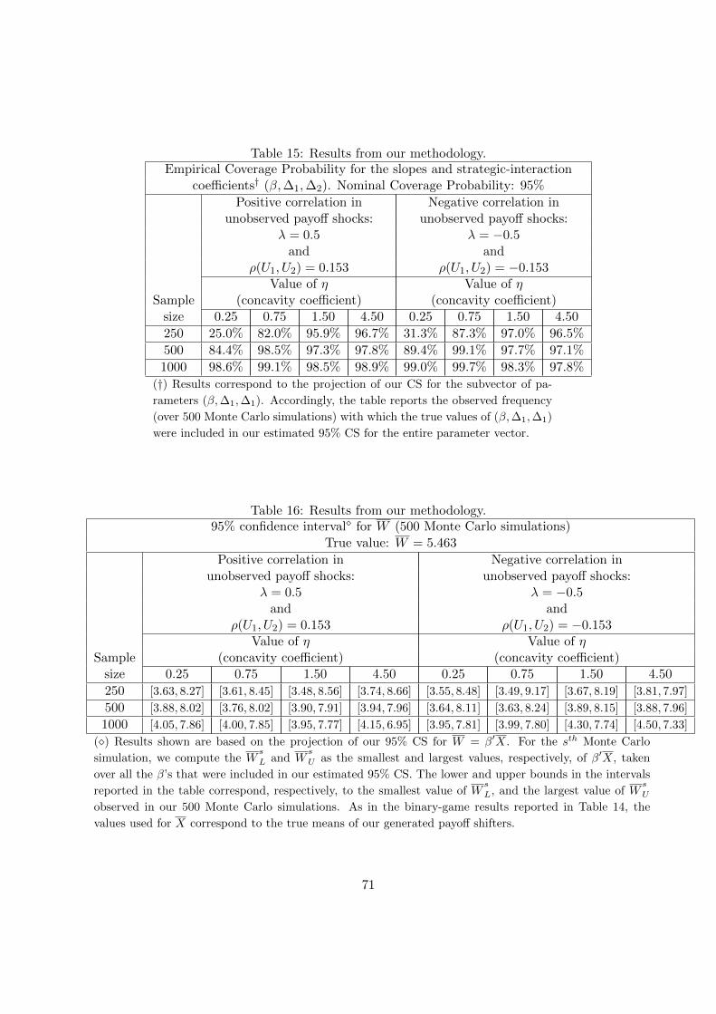
Table 15: Results from our methodology.Empirical Coverage Probability for the slopes and strategic-interaction
coefficients† (β,∆1,∆2). Nominal Coverage Probability: 95%
Positive correlation in Negative correlation inunobserved payoff shocks: unobserved payoff shocks:
λ = 0.5 λ = −0.5and and
ρ(U1, U2) = 0.153 ρ(U1, U2) = −0.153Value of η Value of η
Sample (concavity coefficient) (concavity coefficient)size 0.25 0.75 1.50 4.50 0.25 0.75 1.50 4.50
250 25.0% 82.0% 95.9% 96.7% 31.3% 87.3% 97.0% 96.5%
500 84.4% 98.5% 97.3% 97.8% 89.4% 99.1% 97.7% 97.1%
1000 98.6% 99.1% 98.5% 98.9% 99.0% 99.7% 98.3% 97.8%
(†) Results correspond to the projection of our CS for the subvector of pa-
rameters (β,∆1,∆1). Accordingly, the table reports the observed frequency
(over 500 Monte Carlo simulations) with which the true values of (β,∆1,∆1)
were included in our estimated 95% CS for the entire parameter vector.
Table 16: Results from our methodology.95% confidence interval for W (500 Monte Carlo simulations)
True value: W = 5.463
Positive correlation in Negative correlation inunobserved payoff shocks: unobserved payoff shocks:
λ = 0.5 λ = −0.5and and
ρ(U1, U2) = 0.153 ρ(U1, U2) = −0.153Value of η Value of η
Sample (concavity coefficient) (concavity coefficient)size 0.25 0.75 1.50 4.50 0.25 0.75 1.50 4.50
250 [3.63, 8.27] [3.61, 8.45] [3.48, 8.56] [3.74, 8.66] [3.55, 8.48] [3.49, 9.17] [3.67, 8.19] [3.81, 7.97]
500 [3.88, 8.02] [3.76, 8.02] [3.90, 7.91] [3.94, 7.96] [3.64, 8.11] [3.63, 8.24] [3.89, 8.15] [3.88, 7.96]
1000 [4.05, 7.86] [4.00, 7.85] [3.95, 7.77] [4.15, 6.95] [3.95, 7.81] [3.99, 7.80] [4.30, 7.74] [4.50, 7.33]
() Results shown are based on the projection of our 95% CS for W = β′X. For the sth Monte Carlo
simulation, we compute the Ws
L and Ws
U as the smallest and largest values, respectively, of β′X, taken
over all the β’s that were included in our estimated 95% CS. The lower and upper bounds in the intervals
reported in the table correspond, respectively, to the smallest value of Ws
L, and the largest value of Ws
U
observed in our 500 Monte Carlo simulations. As in the binary-game results reported in Table 14, the
values used for X correspond to the true means of our generated payoff shifters.
71