T82 978-4-86348-717-8 ©2019 JSAP 2019 Symposium on VLSI Technology Digest of Technical Papers

T8-1Inference of Long-Short Term Memory networks at software-equivalent

accuracy using 2.5M analog Phase Change Memory devicesH. Tsai, S. Ambrogio, C. Mackin, P. Narayanan, R. M. Shelby, K. Rocki, A. Chen and G. W. BurrIBM Research–Almaden, 650 Harry Road, San Jose, CA 95120, Tel: (408) 927–2073, E-mail: htsai@us.ibm.com

AbstractWe report accuracy for forward inference of long-short-term-memory

(LSTM) networks using weights programmed into the conductances of>2.5M phase-change memory (PCM) devices. We demonstrate strate-gies for software weight-mapping and programming of hardware analogconductances that provide accurate weight programming despite signifi-cant device variability. Inference accuracy very close to software-modelbaselines is achieved on several language modeling tasks.

Keywords: PCM, LSTM, forward inference, in-memory computingIntroduction

Deep neural network (DNN) computations in analog memory havemade significant progress, recently achieving software-equivalent accu-racy with weights stored in non-volatile memory arrays [1], [2]. Fully-connected (FC) networks, composed of the FC-layers that are particu-larly well-suited for acceleration using in-memory analog computing [3],have been mostly eclipsed in modern DNN applications. But recurrentneural networks (RNN), such as Long-Short-Term-Memory (LSTM),are widely used — for language modeling, speech recognition, transla-tion, and sequence classification — and primarily consist of FC-layers(plus a few element-wise vector operations). Due to the recurrent natureof LSTMs, analog device requirements for LSTMs are more stringent[4] than for FC-networks. To date, experimental demonstrations ofLSTMs in analog memory have been limited by hardware constraints tovery small networks [5]. In this paper, we study the inference accuracyof larger LSTM networks using a mixed-hardware-software experiment[1], where synaptic weights are programmed into a 90nm-node phasechange memory (PCM) array with 4M mushroom-cell devices, whileall neuron functionalities are simulated in software. We use the weightmapping scheme in Fig.1 to map LSTM networks for language modelingtasks using two datasets, including the Penn Tree Bank (PTB) dataset, awidely-used LSTM software benchmark.

LSTM Network and DatasetThe 2-layer LSTM network used in this paper is shown in Fig. 2.

A fully connected embedding layer converts characters or words usinga ‘one-hot’ encoding x0(t) into an embedding vector, x(t), with thesame size as the hidden layer. x(t) is then passed to a 2-layer LSTMwith a recurrent hidden state, h(t), in each layer. Output y(t) is thencomputed from the hidden state in the second layer, h2(t), through afully-connected output layer. Fig. 3a shows weight distributions forsoftware-trained models using two datasets: the book ‘Alice in Wonder-land’ (character-based) with a smaller model (50 hidden units) and thePTB (word-based) dataset (hidden layer size of 200). Since softwareweights span different ranges, different scaling factors are chosen to mapthe weights into the same ‘sensitive region’ of analog conductances [6].

To assess the impact of weight-programming errors, conductancevalues are individually measured from the hardware, and LSTM activa-tions are calculated in software (using the equations in Figs. 1 and 4).Future in-memory analog computing circuitry will efficiently and rapidlyperform these multiply-accumulate operations in the analog domain atthe weight locations, but expected DNN performance for such hardwarecan be evaluated by the present experiment, as follows. For languagemodeling, as each character/word is presented, the LSTM network pre-dicts the probability — quantified by softmax(y(t)) — of the nextcharacter/word in the sequence. This prediction can be compared to theactual next input vector, x0(t+1). ‘Accuracy’ of the model is quantifiedby cross-entropy loss or perplexity – lower loss (perplexity) indicatesthat correct answers are being predicted with higher probability.

Programming PCM Conductances and WeightsFig. 5 compares two strategies for efficient programming in the

presence of device variabilities. One strategy applies SET pulses with

steadily increasing compliance current to reach the target analog conduc-tance. With this method, PCM conductance is non-monotonic, decreas-ing sharply as each device reaches its RESET condition. In contrast,applying RESET pulses with steadily decreasing compliance current ismore tolerant of device variability and offers better precision at low con-ductance values. Iterating these sequences with different pulse-widthhelps further address outlying devices (Fig. 6(b)). Conductance pro-gramming of a single target conductance (Fig.6) and of a simple targetpattern with 32 different levels (Fig.7) show promising results.

Fig. 8 compares weight programming results when using 2 PCMand then 4 PCM devices for weight mapping. Target weight distribu-tions, scaled from software weights into conductance units by α=2.5µS,overlap (Fig. 8a,d) and strongly correlate (Fig. 8b,e) with weights pro-grammed into 2 or 4 PCM devices, with low weight programming error(Fig.8c,f). Successive programming of two conductance pairs with F=4(e,f) significantly reduces weight errors compared to a single pair (b,c).Simple target patterns (Fig.9) also clearly show the benefits of the weightprogramming strategies introduced here.

Impact on LSTM PerformanceFig. 10a summarizes LSTM accuracy results for the Alice in Won-

derland dataset, compared to software baselines (PyTorch & MATLAB).Customized experiments in MATLAB provided an alternate weight-setfor programming, obtained by clipping weight-magnitudes during train-ing to a level that left cross-entropy loss unaffected. The mapping ofthis reduced software-weight range better utilizes available PCM con-ductance levels, and reduces the relative impact of read and write noise.Cross-entropy loss after programming is thus reduced, despite slightlyhigher software loss in the clipped model. Programming only the weightsof the 2-layer LSTM into PCM brings cross-entropy loss even closer tobaseline. Fig.10b shows inference results for the PTB dataset, comparedto PyTorch baseline [7]. (Here only the 2-layer LSTM fits within theavailable PCM array.) LSTM network and dataset sizes are summarizedin Fig. 11a. Fig. 11b puts the inference perplexity of PTB in contextwith state-of-the-art software models [8]. For comparison with the fullmixed-hardware-software results (Fig. 10), inference results with bothconstant (Fig. 11c) and weight-dependent (Fig. 11d, σ values extractedfrom Fig. 9c) added Gaussian noise are shown. Finally, conductancedrift of PCM devices causes LSTM accuracy performance to degrade(Fig.11e), highlighting the importance of PCM device structures knownto offer lower drift [9,10] as well as potentially better conductance-programming accuracy [10].

ConclusionsWe demonstrated analog conductance programming and weight

mapping of LSTM weights into PCM arrays for inference. Write noisewas found to be the primary limiting factor. Training and mappingprocedures were shown that can help avoid large weights prone to pro-gramming error. Despite non-ideality and variability in PCM arrays,inference results close to software baselines were achieved on LSTMnetworks of competitive-size.

References[1] G. W. Burr et. al., IEDM, T29-5 (2014).[2] S. Ambrogio et. al., Nature, 558, 60-67 (2018).[3] T. Gokmen et. al., Frontiers in Neuroscience, 10, 333 (2016).[4] T. Gokmen et. al., Frontiers in Neuroscience, 12, 745 (2018).[5] C. Li et. al., Nat. Machine Intelligence, 1, 49-57 (2019).[6] C. Mackin et. al., Adv. Electr. Mater., submitted (2019).[7] https://github.com/deeplearningathome/pytorch-language-model[8] S. Merity et. al., https://arxiv.org/abs/1708.02182, (2017).[9] S. Kim et al., IEDM, 30-7 (2013).[10] I. Giannopoulos et al., IEDM, 27-7 (2018).

T832019 Symposium on VLSI Technology Digest of Technical Papers

W = G+ - G- +

G+ G– g+ g-

Most Significant Pair(MSP)

Least Significant Pair(LSP)

g+ - g-

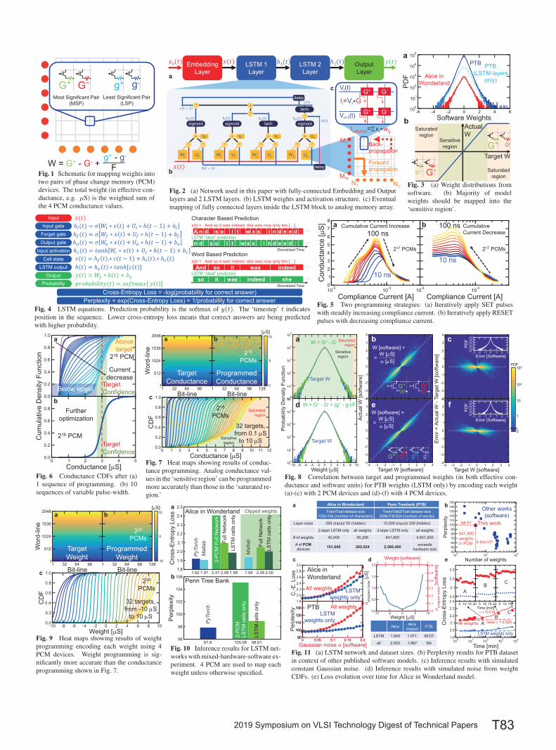
FFig. 1 Schematic for mapping weights intotwo pairs of phase change memory (PCM)devices. The total weight (in effective con-ductance, e.g. µS) is the weighted sum ofthe 4 PCM conductance values.

Embedding Layer

LSTM 1 Layer

LSTM 2 Layer

Output Layer

𝑥𝑥0(𝑡𝑡) 𝑥𝑥(𝑡𝑡) ℎ1(𝑡𝑡) ℎ2(𝑡𝑡) 𝑦𝑦(𝑡𝑡)

G+ G-

G+ G-Vi+1(t)

Vi(t)

Ii=Vi×G

Icolumn=Sxi×wij

a

b

c

N1

M1

MmNn

Forwardpropagation

Back-propagation

Wf Uf

bf

+

ℎ𝑓𝑓(𝑡𝑡)

Wi Ui

bi

+

ℎ𝑖𝑖(𝑡𝑡)

Wc Uc

bc

+

ℎ𝑐𝑐(𝑡𝑡)

Wo Uo

bo

+

ℎ𝑜𝑜(𝑡𝑡)

* * * * * * * *

sigmoid sigmoid tanh sigmoid

𝑥𝑥(𝑡𝑡) ℎ 𝑡𝑡 − 1

𝑐𝑐 𝑡𝑡 − 1 .*

.*

+tanh

𝑐𝑐 𝑡𝑡

.*ℎ(𝑡𝑡)

delay

delay

Fig. 2 (a) Network used in this paper with fully-connected Embedding and Outputlayers and 2 LSTM layers. (b) LSTM weights and activation structure. (c) Eventualmapping of fully connected layers inside the LSTM block to analog memory array.

a

Alice in Wonderland

PTB

G+ G–

G+ G–

b

Target W

Actual W

Sensitive region

Saturated region

Saturated region

PTB (LSTM layers

only)

Fig. 3 (a) Weight distributions fromsoftware. (b) Majority of modelweights should be mapped into the‘sensitive region’.

x(t) = And so it was indeed: she was now only ten […]

LSTM “ideal” predictionA n d s o i t w a s i n d e e d :

n d s o i t w a s i n d e e d :

And so it was indeed

so it was indeed she

ℎ𝑓𝑓(𝑡𝑡) = 𝜎𝜎 𝑊𝑊𝑓𝑓 ∗ 𝑥𝑥 𝑡𝑡 + 𝑈𝑈𝑓𝑓 ∗ ℎ(𝑡𝑡 − 1) + 𝑏𝑏𝑓𝑓

𝑐𝑐(𝑡𝑡) = ℎ𝑓𝑓 𝑡𝑡 .∗ 𝑐𝑐(𝑡𝑡 − 1) + ℎ𝑖𝑖 𝑡𝑡 .∗ ℎ𝑐𝑐(𝑡𝑡)ℎ 𝑡𝑡 = ℎ𝑜𝑜 𝑡𝑡 .∗ 𝑡𝑡𝑡𝑡𝑡𝑡ℎ[𝑐𝑐 𝑡𝑡 ]𝑦𝑦(𝑡𝑡) = 𝑊𝑊𝑦𝑦 ∗ ℎ(𝑡𝑡) + 𝑏𝑏𝑦𝑦

ℎ𝑖𝑖(𝑡𝑡) = 𝜎𝜎 𝑊𝑊𝑖𝑖 ∗ 𝑥𝑥 𝑡𝑡 + 𝑈𝑈𝑖𝑖 ∗ ℎ(𝑡𝑡 − 1) + 𝑏𝑏𝑖𝑖

ℎ𝑜𝑜(𝑡𝑡) = 𝜎𝜎 𝑊𝑊𝑜𝑜 ∗ 𝑥𝑥 𝑡𝑡 + 𝑈𝑈𝑜𝑜 ∗ ℎ(𝑡𝑡 − 1) + 𝑏𝑏𝑜𝑜ℎ𝑐𝑐(𝑡𝑡) = 𝑡𝑡𝑡𝑡𝑡𝑡ℎ 𝑊𝑊𝑐𝑐 ∗ 𝑥𝑥 𝑡𝑡 + 𝑈𝑈𝑐𝑐 ∗ ℎ(𝑡𝑡 − 1) + 𝑏𝑏𝑐𝑐

Input gateForget gateOutput gate

Input activationCell state

LSTM output

Input 𝑥𝑥(𝑡𝑡)

Output

Discretized Time

…

…

Character Based Prediction

Discretized Time

…

…

Word Based Predictionx(t) = And so it was indeed: she was now only ten […]

LSTM “ideal” prediction

Cross-Entropy Loss = -log(probability for correct answer) Perplexity = exp(Cross-Entropy Loss) = 1/probability for correct answer

Probability 𝑝𝑝𝑝𝑝𝑝𝑝𝑏𝑏𝑡𝑡𝑏𝑏𝑝𝑝𝑝𝑝𝑝𝑝𝑡𝑡𝑦𝑦(𝑡𝑡) = 𝑠𝑠𝑝𝑝𝑠𝑠𝑡𝑡𝑠𝑠𝑡𝑡𝑥𝑥[ 𝑦𝑦 𝑡𝑡 ]

Fig. 4 LSTM equations. Prediction probability is the softmax of y(t). The ‘timestep’ t indicatesposition in the sequence. Lower cross-entropy loss means that correct answers are being predictedwith higher probability.

a bCumulative Current Increase Cumulative Current Decrease

10 ns

100 ns100 ns

10 ns217 PCMs 217 PCMs

Fig. 5 Two programming strategies: (a) Iteratively apply SET pulseswith steadily increasing compliance current. (b) Iteratively apply RESETpulses with decreasing compliance current.

TargetConfidence

216 PCM

Abovetarget

Current decrease

a

TargetConfidence

216 PCM

Further optimization

b

Below target

Fig. 6 Conductance CDFs after (a)1 sequence of programming. (b) 10sequences of variable pulse-width.

32 targets, from 0.1 mS

to 10 mSSensitive region

Programmed Conductance

Target Conductance

a b

0

5

10[mS]

c218

PCMs

218

PCMs

Saturated region

Fig. 7 Heat maps showing results of conduc-tance programming. Analog conductance val-ues in the ‘sensitive region’ can be programmedmore accurately than those in the ‘saturated re-gion.’

0

10

103PDF

e

c

f

G+ G–

G+ G– g+ g-

102

b

d

Target W

W = G+ - G- + (g+ - g-)/F

W = G+ - G-

Target W

a Saturated region

Sensitive region

≈≈

W [software] =

=W [mS]a [mS]

W [software] =

=W [mS]a [mS]

1

Fig. 8 Correlation between target and programmed weights (in both effective con-ductance and software units) for PTB weights (LSTM only) by encoding each weight(a)-(c) with 2 PCM devices and (d)-(f) with 4 PCM devices.

Programmed Weight

Target Weight

a b

-10

0

10[mS]

32 targets, from -10 mS

to 10 mS

c

220

PCMs

220

PCMs

Fig. 9 Heat maps showing results of weightprogramming encoding each weight using 4PCM devices. Weight programming is sig-nificantly more accurate than the conductanceprogramming shown in Fig. 7.

PyT

orch

Mat

lab Fu

ll N

etw

ork

Alice in Wonderland

Penn Tree Bank

a

b

LSTM

cel

ls o

nly

Mat

lab

Full

Net

wor

kLS

TM c

ells

onl

y

1.92 1.91 2.09 1.99 1.94 2.05 2.00

PyT

orch

2-PC

M

LSTM

cel

ls o

nly

LSTM

cel

ls o

nly

97.9 105.08 98.91

2-PC

M F

ull N

etw

ork

2.41

Clipped weights

Fig. 10 Inference results for LSTM net-works with mixed-hardware-software ex-periment. 4 PCM are used to map eachweight unless otherwise specified.

Alice in Wonderland Penn Treebank (PTB)

Train/Test dataset size135k/15k (number of characters)

Train/Valid/Test dataset size929k/73k/82k (number of words)

Layer sizes 256 (input)/ 50 (hidden) 10,000 (input)/ 200 (hidden)

2-layer LSTM only all weights 2-layer LSTM only all weights

# of weights 40,400 66,256 641,600 4,651,600

# of PCM devices 161,600 265,024 2,566,400 exceeds

hardware size

a b

e

This work

Other works(software)

c

Alice Alice clipped PTB

LSTM 1.949 1.971 99.07

all 2.053 1.997 NA

d

98.91

641,600 weights in PCM 4.64x106

All weights LSTM weights onlyAll weights

LSTM weights only

Alice in Wonderland

PTB

AB

C

AB

C

All weights

LSTM weights only

n = 0.018

Ideal n = 0.005

Fig. 11 (a) LSTM network and dataset sizes. (b) Perplexity results for PTB datasetin context of other published software models. (c) Inference results with simulatedconstant Gaussian noise. (d) Inference results with simulated noise from weightCDFs. (e) Loss evolution over time for Alice in Wonderland model.