inferential model predictive control of …etd.lib.metu.edu.tr/upload/12607497/index.pdf ·...
TRANSCRIPT
INFERENTIAL MODEL PREDICTIVE CONTROL OF
POLY(ETHYLENE TEREPHTHALATE) DEGRADATION DURING EXTRUSION
A THESIS SUBMITTED TO THE GRADUATE SCHOOL OF NATURAL AND APPLIED SCIENCES
OF MIDDLE EAST TECHNICAL UNIVERSITY
BY
MURAT OLUŞ ÖZBEK
IN PARTIAL FULFILLMENT OF THE REQUIREMENTS FOR
THE DEGREE OF MASTER OF SCIENCE IN
CHEMICAL ENGINEERING
AUGUST 2006

2
Approval of the Graduate School of Natural and Applied Sciences.
___________________________
Prof Dr. Canan Özgen
Director
I certify that this thesis satisfies all the requirements as a thesis for the degree of Master of
Science.
___________________________
Prof. Dr. Nurcan Baç
Head of Department
This is to certify that we have read this thesis and that in our opinion it is fully adequate, in
scope and quality, as a thesis for the degree of Master of Science.
__________________________ __________________________
Assoc. Prof. Dr. Göknur Bayram Prof. Dr. Canan Özgen
Co-supervisor Supervisor
Examining Committee Members
Prof. Dr. Güngör Gündüz
(METU, CHE)________________________
Prof. Dr. Canan Özgen
(METU, CHE)________________________
Doç Dr. Göknur Bayram
(METU, CHE)________________________
Doç. Dr. Naime Aslı Sezgi
(METU, CHE)________________________
Prof. Dr. Kemal Leblebicioğlu
(METU, EE)________________________

iii
PLAGIARISM
I hereby declare that all information in this document has been obtained and presented in
accordance with academic rules and ethical conduct. I also declare that, as required by
these rules and conduct, I have fully cited and referenced all material and results that are
not original to this work.
Name, Last name:
Signature :
iv
ABSTRACT
INFERENTIAL MODEL PREDICTIVE CONTROL OF POLY(ETHYLENE TEREPHTHALATE) DEGRADATION
DURING EXTRUSION
Özbek, Murat Oluş
M. S., Department of Chemical Engineering
Supervisor: Prof. Dr. Canan Özgen
Co-Supervisor: Assoc. Prof. Dr. Göknur Bayram
August 2006, 91 pages
Poly(ethylene terephthalate), PET, which is commonly used as a packaging material, is not
degradable in nature. As an issue of sustainable development it must be recycled and
converted into other products. During this process, extrusion is an important unit operation.
In extrusion process, if the operating conditions are not controlled, PET can go under
degradation, which results in the loss of some mechanical properties.
In order to overcome the degradation of recycled PET (RPET), this study aims the control of
the extrusion process. Dynamic models of the system for control purposes are obtained by
experimental studies. In the experimental studies, screw speed, feed rate and barrel
temperatures are taken as process variables in the ranges of 50 – 500 rpm, 3.85 – 8.16
g/min and 270 – 310 oC respectively. Singular value decomposition (SVD) technique is used
for the best pairing between the manipulated – controlled variables, where screw speed is
taken as the manipulated variable and molecular weight of the product is taken as the
controlled variable. PID and model predictive controller (MPC) are designed utilizing the
dynamic models in the feedback inferential control algorithm. In the simulation studies, the
performance of the designed inferential control system, where molecular weight (Mv) of the
product is estimated from the measured intrinsic viscosity ([η]) of the product, is
investigated.

v
The controller utilizing PID and MPC control algorithms are found to be robust and
satisfactory in tracking the given set points and eliminating the effects of the disturbances.
Keywords: extrusion, modeling, MPC, inferential control, PET recycling.
vi
ÖZ
EKSTRÜZYON İŞLEMİNDE
POLY(ETİLEN TEREFTALAT) BOZUNMASININ
ALGISAL MODEL ÖNGÖRÜMLÜ DENETLEÇ İLE DENETLENMESİ
Özbek, Murat Oluş
Yüksek Lisans, Kimya Mühendisliği Bölümü
Tez Yöneticisi: Prof. Dr. Canan Özgen
Ortak Tez Yöneticisi: Doç. Dr. Göknur Bayram
Ağustos 2006, 91 sayfa
Genellikle, paketleme malzemesi olarak kullanılan polietilen tereftalat’ın (PET) doğada bozunma özelliği
yoktur. Bu nedenle, sürdürülebilir gelişme sürecinde PET’in geri kazanılması ve yararlı ürünlere
dönüştürülmesi gerekir. Bu işleme süreçlerinde ekstrüzyon yöntemi önemli bir temel işlemdir. Ancak,
ekstrüzyon sürecinde koşulların iyi ayarlanamadığı durumlarda, PET, bozunmaya (degradation)
uğrayabilir ve bunun sonucunda mekanik bazı özelliklerini kaybedebilir.
Bu çalışmada, PET’in bozunmasının önlenebilmesi için ekstrüzyon sürecinin denetimi amaçlanmıştır.
Denetimde kullanılmak üzere, sistemin dinamik modelleri deneysel çalışmalar yardımıyla elde edilmiştir.
Deneysel çalışmalarda süreç değişkenleri olarak 270 - 310 oC aralığında kovan sıcaklığı (T), 50 – 500
dev/dak aralığında vida hızı (SS), 3.85 - 8.16 g/dak aralığında besleme oranı (FR) seçilmiştir. En iyi
ayarlanan-denetlenen değişken eşleştirmesi için Tekil Değer Ayrıştırma (SVD) tekniği kullanılmış ve
ayarlanan değişken olarak vida hızı (SS), denetlenen değişken olarak ürünün molekül ağırlığı (Mv)
seçilmiştir. Elde edilen dinamik modellerle geleneksel (PID) ve model öngörümlü denetleçler (MÖD)
tasarlanmış ve geri beslemeli, algısal denetim algoritmasında kullanılmıştır. Benzetim çalışmalarında,
ürünün molekül ağırlığının (Mv) ölçülen içsel viskozite ([η]) değerlerinden tahmin edildiği algısal
denetim yapısının performansı incelenmiştir.
PID ve MÖD denetim algoritmaları kullanan denetleçlerin hem gürbüz hem de ayar noktası izleme ve
bozan etkenin etkisini uzaklaştırma konularında başarılı oldukları irdelenmiştir.

vii
Anahtar Sözcükler: ekstrüzyon, modelleme, model öngörümlü denetim, algısal denetim, geri
dönüşümlü PET.

viii
Dedicated to all my beloved ones…

ix
ACKNOWLEDGMENTS
First of all, I wish to express my sincere gratitude to my supervisor Prof. Dr. Canan Özgen
and co-supervisor Assoc. Prof. Göknur Bayram for their valuable suggestions, guidance and
understanding throughout my graduate study.
I would like to thank to all of my colleagues; especially to Salih Obut, Almıla Bahar, İsmail
Doğan, Hatice Ceylan, Sertan Yeşil, Güralp Özkoç, Işıl Işık, Özcan Köysüren and Mert Kılınç
for their help and support during my graduate study.
I would like to thank to all my co-workers in Middle East Technical University Graduate
School of Natural and Applied Sciences for their support and understanding.
Last but not least, I wish to express my deepest thanks to my family for their great support,
encouragement, and patience throughout my all education.
x
TABLE OF CONTENTS
PLAGIARISM ................................................................................................................... iii
ABSTRACT......................................................................................................................iv
ÖZ .................................................................................................................................vi
ACKNOWLEDGMENTS......................................................................................................ix
TABLE OF CONTENTS...................................................................................................... x
LIST OF TABLES............................................................................................................. xii
LIST OF FIGURES.......................................................................................................... xiv
NOMENCLATURE.......................................................................................................... xvii
CHAPTER
1. INTRODUCTION.......................................................................................................... 1
2. LITERATURE SURVEY .................................................................................................. 3
2.1 Extrusion, Extruder Modeling and Extruder Control................................................... 3
2.2 PET Recycling and PET Degradation ........................................................................ 8
2.3 Model Predictive Control (MPC) ..............................................................................10
2.4 Inferential Control .................................................................................................12
2.5 Singular Value Decomposition (SVD) ......................................................................13
3. BACKGROUND INFORMATION ON PET AND CONTROL TECHNIQUES ............................14
3.1 Poly(ethylene terephthalate) (PET).........................................................................14
3.1.1 Recycling........................................................................................................15
3.1.2 Degradation....................................................................................................16
3.2 Control Techniques ...............................................................................................18
3.2.1 MPC ...............................................................................................................18
3.2.1.1 MPC Algorithm..........................................................................................18
3.2.1.2 Constrained MPC ......................................................................................20
3.2.3 Inferential Control ..............................................................................................21
3.3 Singular Value Decomposition (SVD) ......................................................................22
4. EXPERIMENTAL STUDIES............................................................................................24
4.1 Properties of RPET and Trifluoroacetic Acid (TFA) ...................................................24
4.2 Experimental Setup ...............................................................................................25
4.3 Experimental Procedure.........................................................................................27
xi
4.3.1 Preliminary Experiments ..................................................................................27
4.3.2 Steady State Experiments................................................................................28
4.3.3 Dynamic Experiments......................................................................................29
5. RESULTS AND DISCUSSIONS......................................................................................31
5.1 Preliminary Experimental Results............................................................................31
5.2 Steady State Experimental Results .........................................................................33
5.3 Dynamic Experimental Results ...............................................................................36
5.4 Modeling Studies...................................................................................................39
5.4.1 Modeling Technique 1: Single Transfer Functions..............................................41
5.4.2 Modeling Technique 2: Dual Transfer Functions ................................................44
5.4.3 Modeling Technique 3: Discrete Convolution Models..........................................46
5.5 Control Studies .....................................................................................................49
5.5.1 Singular Value Decomposition..........................................................................49
5.5.2 Design of Control Scheme ...............................................................................51
5.5.3 PID Control.....................................................................................................52
5.5.4 Model Predictive Control (MPC) ........................................................................54
5.5.4.1 Process Models for MPC ............................................................................54
5.5.4.2 MPC Tuning..............................................................................................55
5.5.5 Robustness Analysis ........................................................................................63
6. CONCLUSIONS...........................................................................................................72
REFERENCES .................................................................................................................73
APPENDICES
A. MOLECULAR WEIGHT DETERMINATION......................................................................77
B. CALIBRATION FOR RESIDENCE TIME AND FEED RATE.................................................79
C. EXPERIMENTAL DATA ................................................................................................82
D. PID CONTROL LOOP AND PROGRAM CODES ...............................................................84
E. SAMPLE CALCULATIONS.............................................................................................88
xii
LIST OF TABLES
TABLES
Table 3.1: Minimum requirements for RPET flakes to be reprocessed [Ajawa and Pavel,
2005]. ....................................................................................................................16
Table 4.1: Properties of RPET resin (AdvanSA).................................................................25
Table 4.2: Step changes given to the process variables. ...................................................29
Table 5.1: Measured intrinsic viscosity and molecular weight of unprocessed RPET. ...........32
Table 5.2: Results of consistency check ...........................................................................36
Table 5.3: Single transfer function models and their normalized IAE scores. ......................42
Table 5.4: Dual transfer function models and their normalized IAE scores. ........................44
Table 5.5: PID settings utilizing modified Z-N method (Some Overshoot) [Seborg et al.,
1989], and normalized IAE scores of set point tracking (Figure 5.19)..........................52
Table 5.6: Fine tuned PID settings for PID+ and PID-........................................................53
Table 5.7: The magnitudes and the time of changes of the given set point changes...........54
Table 5.8: MPC tuning parameters. .................................................................................56
Table 5.9: Normalized IAE scores of controllers throughout set point tracking....................57
Table 5.10: Normalized IAE scores and settling times of controllers in disturbance rejection
performances. .........................................................................................................60
Table 5.11: Normalized IAE scores of controllers throughout set point tracking (10%
increase in model gains). .........................................................................................65
Table 5.12: Normalized IAE scores of controllers throughout set point tracking (10%
decrease in model gains). ........................................................................................65
Table 5.13: Normalized IAE scores and settling times of controllers in disturbance rejection
performances (10% increase in model gains). ...........................................................70
Table 5.14: Normalized IAE scores and settling times of controllers in disturbance rejection
performances (10% decrease in models gains). ........................................................71
Table B.1: Average residence times for studied screw speeds. ..........................................79
Table B.2: Flow rate calibration data for studied feed rate settings....................................80
Table C.1: Molecular weight (g/gmol), Mv, change for different SS and FR values at 270 oc.
..............................................................................................................................82
Table C.2: Molecular weight (g/gmol), Mv, change for different SS and FR values at 290 oc.
..............................................................................................................................82

xiii
Table C.3: Molecular weight (g/gmol), Mv, change for different SS and FR values at 310 oc.
..............................................................................................................................82
Table C.4: Mv (g/gmol) change with SS, FR and T (dynamic runs).....................................83
Table E.1: Experimental data (an example)......................................................................88
Table E.2: Reduced viscosity for different concentrations..................................................89
Table E.3: Ultimate gains and ultimate periods of positive and negative PID-model pairs....90
Table E.4: Original and modified Ziegler-Nichols settings for PID controllers [Seborg et al.,
1989]. ....................................................................................................................91
xiv
LIST OF FIGURES
FIGURES
Figure 3.1: PET synthesis reactions: (a) trans-esterification reaction and (b) condensation
reaction [Ajawa and Pavel, 2005]. ............................................................................15
Figure 3.2: Thermal degradation of PET [Karayannidis et al., 2000]. .................................17
Figure 3.3: Acid alcohol condensation of PET [Karayannidis and Psalida, 2000]..................17
Figure 3.4: Open loop step response of a linear plant [Seborg et al., 1989]. ......................18
Figure 3.5: Block diagram for inferential control loop........................................................21
Figure 4.1: Molecular formula of trifluoroacetic acid (TFA). ...............................................24
Figure 4.2: Extruder used for experiments. ......................................................................26
Figure 4.3: Schematic drawing for the experimental setup. ...............................................26
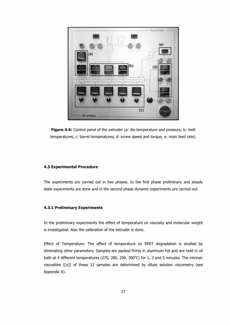
Figure 4.4: Control panel of the extruder (a: die temperature and pressure, b: melt
temperatures, c: barrel temperatures, d: screw speed and torque, e: main feed rate). 27
Figure 5.1: The effect of temperature on molecular weight of RPET. .................................32
Figure 5.2: Effect of SS and FR on Mv at T = 270 oC.........................................................34
Figure 5.3: Effect of SS and FR on Mv at T = 290 oC.........................................................34
Figure 5.4: Effect of SS and FR on Mv at T = 310 oC.........................................................35
Figure 5.5: System responses to (a) positive (+25 rpm) and (b) negative (-50 rpm) steps on
screw speed............................................................................................................37
Figure 5.6: System responses to (a) positive (+1.04 g/min) (+25) and (b) negative (-1.42
g/min) (-25) steps on feed rate. ...............................................................................38
Figure 5.7: System responses to (a) positive (+20 oC) and (b) negative (-20 oC) steps on
temperature. ...........................................................................................................38
Figure 5.8: Model representation of the system................................................................40
Figure 5.9: Plant and model responses to a (a) positive and (b) negative unit step changes
in SS (single transfer function case)..........................................................................41
Figure 5.10: Plant and model responses to a (a) positive and (b) negative unit step changes
in FR (single transfer function case)..........................................................................43
Figure 5.11: Plant and model responses to a (a) positive and (b) negative unit step changes
in T (single transfer function case). ..........................................................................43
xv
Figure 5.12: Plant and model responses to a (a) positive and (b) negative unit step changes
in SS (dual transfer functions case). .........................................................................45
Figure 5.13: Plant and model responses to a (a) positive and (b) negative unit step changes
in FR (dual transfer functions case). .........................................................................45
Figure 5.14: Plant and model responses to a (a) positive and (b) negative unit step changes
in T (dual transfer functions case). ...........................................................................46
Figure 5.15: Plant and model responses to a (a) positive and (b) negative unit step changes
in SS (discrete convolution models case)...................................................................47
Figure 5.16: Plant and model responses to a (a) positive and (b) negative unit step changes
in FR (discrete convolution models case)...................................................................48
Figure 5.17: Plant and model responses to a (a) positive and (b) negative unit step changes
in T (discrete convolution models case). ...................................................................48
Figure 5.18: Designed control system..............................................................................52
Figure 5.19: Set point tracking of PID controllers of (a) positive and (b) negative models,
tuned using modified Z-N settings (Some Overshoot) [Seborg et al., 1989].................53
Figure 5.20: Responses of ARX models to (a) positive and (b) negative unit step changes in
SS. .........................................................................................................................55
Figure 5.21: Set point tracking responses of PID and MPC. ...............................................56
Figure 5.22: Disturbance rejection responses of PID and MPC (+25 or +1.04 g/gmol step
disturbance on FR). .................................................................................................57
Figure 5.23: Disturbance rejection responses of PID and MPC (-25 or -1.42 g/gmol step
disturbance on FR). .................................................................................................58
Figure 5.24: Disturbance rejection responses of PID and MPC (+10 oC step disturbance on
T)...........................................................................................................................59
Figure 5.25: Disturbance rejection responses of PID and MPC (-10 oC step disturbance on T).
..............................................................................................................................59
Figure 5.26: Disturbance rejection responses of PID and MPC (+12.5 or +0.57 g/gmol step
disturbance on FR). .................................................................................................61
Figure 5.27: Disturbance rejection responses of PID and MPC (-12.5 or -0.71 g/gmol step
disturbance on FR). .................................................................................................61
Figure 5.28: Disturbance rejection responses of PID and MPC (+20 oC step disturbance on
T)...........................................................................................................................62
Figure 5.29: Disturbance rejection responses of PID and MPC (-20 oC step disturbance on T).
..............................................................................................................................62
Figure 5.30: Set point tracking responses of PID and MPC (10% increase in model gains). .64
Figure 5.31: Set point tracking responses of PID and MPC (10% decrease in model gains).64
xvi
Figure 5.32: Disturbance rejection responses of PID and MPC (+1.04 g/gmol step
disturbance on FR) (10% increase in model gains). ...................................................66
Figure 5.33: Disturbance rejection responses of PID and MPC (-1.42 g/gmol step disturbance
on FR) (10% increase in model gains). .....................................................................66
Figure 5.34: Disturbance rejection responses of PID and MPC (+1.04 g/gmol step
disturbance on FR) (10% decrease in model gains). ..................................................67
Figure 5.35: Disturbance rejection responses of PID and MPC (-1.42 g/gmol step disturbance
on FR) (10% decrease in model gains). ....................................................................67
Figure 5.36: Disturbance rejection responses of PID and MPC (+10 oC step disturbance on T)
(10% increase in model gains). ................................................................................68
Figure 5.37: Disturbance rejection responses of PID and MPC (-10 oC step disturbance on T)
(10% increase in model gains). ................................................................................69
Figure 5.38: Disturbance rejection responses of PID and MPC (+10 oC step disturbance on T)
(10% decrease in model gains). ...............................................................................69
Figure 5.39: Disturbance rejection responses of PID and MPC (-10 oC step disturbance on T)
(10% decrease in model gains). ...............................................................................70
Figure A.1: Ostwald and Ubbelohde viscometers. .............................................................78
Figure B.1: Avarage residence times measured at different screw speeds. .........................80
Figure B.2: Feed rate settings and corresponding flow rates (g/min). ................................81
Figure D.1: Feedback control loop for PID controllers designed in SIMULINK. ....................84
Figure E.1: Reduced viscosity change with concentration..................................................90
xvii
NOMENCLATURE
a Step response coefficient
A Coefficient matrix
E Error
E Error vector
FR Feed Rate (g/gmol)
G Steady-state gain matrix
h Impulse response coefficient
K Gain matrix
K Gain value or Mark-Hauwing constant
L Control horizon
m Manipulated variable
M Input vector
Mv Viscosity average molecular weight
Mw Weight average molecular weight
PP Polypropylene
r Set point
R Prediction horizon
SS Screw Speed (rpm)
T Temperature (oC)
U Left singular matrix in SVD
V Right singular matrix in SVD
y Output
Y Output vector
Subscripts:
n Sample number (in means of ∆t)
Superscripts:
c Corrected prediction
d Desired value
p Predicted value
N Normalized value
xviii
Greek Letters:
α Filter value or Mark-Hauwing constant
λ Weighting matrix diagonal element
τ Process transfer function time constant
∆ Increment
ω Weighting matrices
[ ]η Intrinsic viscosity
redη Reduced viscosity
relη Relative viscosity
Σ Sum or Singular value matrix in SVD
Abbreviations:
ANN Artificial Neural Network
ARTD Average Residence Time Distribution
DMC Dynamic Matrix Control
ILR In-line reometer
IMC Internal Model Control
IV Intrinsic Viscosity
LDPE Low Density Polyethylene
MAC Model Algorithmic Control
MFI Melt Flow Index
MI Melt Index
MIMO Multiple Input Multiple Output
MPC Model Predictive Control
MPHC Model Predictive Heuristic Control
MVC Minimum Variance Conroller
PET Poly(ethylene terephthalate)
PVC Polyvinyl chloride
RPET Recycled poly(ethylene terephthalate)
RTD Residence Time Distribution
SISO Single Input Single Output
SSE Single Screw Extruder
STR Self Tuning Regulator
SVD Singular Value Decomposition
TFA Trifluoroacetic acid
TSE Twin Screw Extruder
1
CHAPTER I
INTRODUCTION
PET, which is a thermoplastic resin of polyester family, has become one of the major
packaging materials due to its good barrier and mechanical properties. Due to its non-
degradable nature, PET must be recycled for sustainable development and must be used to
obtain other byproducts. Today, PET is one of the most recycled materials world wide.
The major drawback in PET recycling is the loss of the molecular weight, a phenomenon
known as degradation. Heat, mechanical effects, contaminants and water moisture are the
important factors of degradation. Degradation has an adverse effect on the mechanical
properties of the product. Therefore, degradation amount should be reduced to preserve the
mechanical properties. Molecular weight can be used to express the degradation amount.
Extruders are commonly used machinery in plastics processing and recycling industries.
Previous studies [Incarnato et al., 2000; Spinace et al., 2000; Assadi et al., 2004; Ajawa and
Pawel, 2004] showed that the degradation of RPET is caused mainly by processes taking
place in the extruder. Furthermore, the quality of an extruded product is directly related to
its rheological properties such as melt viscosity of the material in the extruder. Thus,
extrusion process should be controlled in order to reduce the degradation amount.
Previous studies [Parnaby et al., 1975; Smith et al., 1978; Hassan and Parnaby, 1981, Costin
et al., 1982; Yang and Lee, 1986; Tanttu et al., 1989; Pabendiskas et al., 1989; Nied et al.,
2000; Xiao et al., 2001; Previdi et al., 2006] on the control of an extruder or extrusion
process mainly focused on regulating the process parameters like screw speed, barrel
temperatures or barrel/die temperature or pressure on defined preset values. However, in
such a regulation, expert knowledge on the operation and on the relations between the
process conditions and product properties is required. In order to eliminate the requirement
of such an expert knowledge, by using the secondary measurements, an inferential control
2
scheme can be designed for the control of desired product property whose online
measurement is not possible.
Product property is important for the downstream operations of the extruder and can be
kept constant at a desired point by designing a proper control mechanism for the extruder.
Among the different types of controllers, model predictive controller (MPC) has proven itself
worthy and being used in the industry for the last two decades. Although different
algorithms exist for MPC, the name basically refers to a family of controllers in which the
future behavior of the plant is predicted using a dynamic model of the plant and necessary
control actions are calculated in an optimal manner.
In this study, the control of product quality in terms of molecular weight of extruded RPET is
aimed. The system parameters affecting the molecular weight (Mv) are screw speed (SS),
feed rate (FR) and temperature (T). Thus the inputs are considered to be SS, FR and T, and
the output as Mv. The die temperature, die pressure and torque which are additional
parameters are not taken as variables in the scope of this study. Nominal operating point in
term of SS, FR and T, suitable for fiber production is determined by using the steady state
experimental data. Dynamic experiments are conducted to obtain the relations between the
inputs (SS, FR and T) and the output (molecular weight of the extruded product) of the
extruder. These data are used to obtain the dynamic models of the process. An inferential
control scheme is designed to control the molecular weight of the product for different
disturbances by simulation studies by using dynamic models. In the designed control
scheme, performances of PID and MPC controllers are studied.
The outline of this work is as follows. A literature survey on previous studied on related
subjects is given in Chapter 2. Background information about PET and control techniques are
given in Chapter 3. Experimental studies including the set-up and procedures are
summarized in Chapter 4. Chapter 5 includes the results of all the experimental, modeling
and control studies with discussions. Conclusions are given in the last chapter, Chapter 6.
3
CHAPTER II
LITERATURE SURVEY
PET is one of the commonly recycled industrial plastics. However, in order to overcome the
phenomenon of loosing material property during recycling, one option is to control the
process to obtain a product with desired property. Control of product property in an
extrusion process is a challenging one as the aimed product property cannot be measured
online in most of the cases. This problem can be overcome by building an inferential control
scheme by measuring the viscosity of the product on-line and predicting the molecular
weight from this measurement. Furthermore, using a model based controller seems
promising to yield more successful results. A literature survey about these subjects is
presented in this chapter.
2.1 Extrusion, Extruder Modeling and Extruder Control
Parnaby et al. (1975) studied the automatic control of an extruder. Their work mainly
outlines the basics of the development of a feed-forward adaptive predictive control
strategy. Also system identification and modeling were done such as stochastic identification
techniques, step and impulse models. The basic structure for the extruder control scheme
and the interaction between the extruder and the die variables were illustrated. In their
work screw speed was accepted as the manipulated variable and the die pressure, as a
measure of degree of mixing, which indirectly gives the product quality, as the controlled
variable. The melt temperature was also monitored to understand the dynamics better. It is
also stated that by on-line updating the model, small changes in model can be compensated.
Smith et al. (1978) explained the operating characteristics of twins screw extruders (TSE).
The study focused on the interrelationships between the design parameters (such as screw
design, die geometry, feed zone geometry), material properties, and operation variables
4
(such as screw speed, barrel and die temperatures). The effects of these variables and
parameters on the product and product quality during operation are also reviewed. In the
work, first, the effects of the parameters were explained mathematically under certain
assumptions. Finally, these parameter based mathematical models were illustrated for
control purposes. Neither experimental nor simulation studies were carried out. Only the
responses to changes in screw speed and feed rate were illustrated using the obtained
models.
Hassan and Parnaby (1981) experimentally constructed a cascade (hierarchical) control loop
on a laboratory scale extruder and studied the feed-back and feed-forward control
strategies. The constructed system measured barrel and die wall temperatures and
pressures, screw speed and the ‘restrictor valve’ position on the die. Measuring these, the
control system sent set points to screw speed, die restrictor valve, barrel and die wall
temperatures. To achieve this goal, the controller used the constructed model of the
extruder and die behavior, and an optimization function to calculate the control action. Also,
in the work two aims of the extruder control are specified as set point tracking (steady-state
control) and disturbance rejection (dynamic control).
Costin et al. (1982) published a review on the present literature about the dynamic modeling
and control of plasticizing extruder. They developed the subject into three headings, which
were extruder disturbance studies, classical control studies and stochastic control studies. It
was pointed that the previous works were mainly focused on long-term disturbances related
with the melt temperature, melt pressure or extrudate thickness.
Costin et al. (1982) studied the effects of the screw speed on the die pressure and
temperature. System dynamics were modeled as first order with dead time and time series
models. Die pressure was controlled by manipulating screw speed. The disturbance was
introduced to the system as difference in feed material composition. Digital PI, self tuning
regulator (STR) and minimum variance controllers (MVC) were studied and compared. The
results of the study showed that instead of eliminating the disturbances, the STR tuned itself
to eliminate the flight noise, which is caused due to the rotation of the screw.
Yang and Lee (1986) proposed several feedback and feed-forward control methods to
control long term and short term disturbances and evaluated these methods using various
load changes. The aim was to control the extrudate thickness by manipulating the take-up
speed against the screw speed load. A first order model was developed and PI controller
5
with Smith predictor and digital noise filters were tested for load and set-point changes. The
experimental results showed that the control structure was good at set-point changes but its
performance was low at load changes due to the inaccuracy of the model.
Tanttu et al. (1989) planted STR on extruder in simulation level in order to control the start-
up period of the extruder by regulating the barrel temperatures. For mathematical
description of the system a distributed parameter model was used. For parameter estimation
different algorithms were tested. The simulation results showed that STR can be used with a
proper parameter estimation algorithm for the start-up and normal operation.
Pabendinskas et al. (1989) studied the degradation of polypropylene (PP) in a reactive
extrusion process to produce PP with a specified molecular weight (Mw). The measured and
manipulated variables were die pressure drop and initiator concentration, respectively. The
initiator (peroxide) concentration was manipulated via syringe pump. Online measured
viscosity via die pressure drop, and melt flow index (MFI), measured via online rheometer,
were used to determine the amount of degradation. Step tests were performed to find the
relation between the die pressure drop and degradation, and this relation was modeled with
a first order with dead time model. The implemented controller scheme was consisted of a
gain scheduling controller with Smith dead time compensator and a PI controller. The PI
controller was used in a cascade manner to control the syringe pump. The results of the
study indicated that the desired Mw could be achieved by the control of the pressure drop.
Boadhead et al. (1996) developed an in-line rheometer (ILR), which had a ‘partial Couette’
geometry, to reduce the measurement delay, and described its use. The reactive extrusion
process was modeled as a first order with dead time process. PI and minimum variance
controllers were tested. The results showed that there was a considerable dead time in spite
of the ILR advantages. It is also offered that the use of adaptive techniques for such a
system could improve the controller performance, because the tested controllers’
performances were not good due to the non-linearity of the process.
De Ruyck (1997) developed a residence time distribution (RTD) model for a twin screw food
extruder. The model was constructed as series of CSTRs with recycling flows and different
volumes. Effects of the variables (screw profile, screw speed, water supply, feed supply and
die diameter) on RTD were observed experimentally and compared with the model results
and seen to be in agreement. By using the model the effect of different screw designs were
also studied.
6
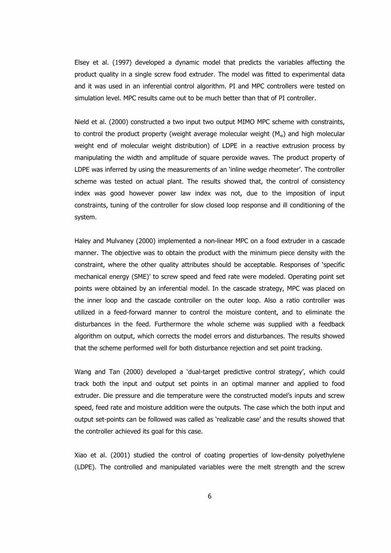
Elsey et al. (1997) developed a dynamic model that predicts the variables affecting the
product quality in a single screw food extruder. The model was fitted to experimental data
and it was used in an inferential control algorithm. PI and MPC controllers were tested on
simulation level. MPC results came out to be much better than that of PI controller.
Nield et al. (2000) constructed a two input two output MIMO MPC scheme with constraints,
to control the product property (weight average molecular weight (Mw) and high molecular
weight end of molecular weight distribution) of LDPE in a reactive extrusion process by
manipulating the width and amplitude of square peroxide waves. The product property of
LDPE was inferred by using the measurements of an ‘inline wedge rheometer’. The controller
scheme was tested on actual plant. The results showed that, the control of consistency
index was good however power law index was not, due to the imposition of input
constraints, tuning of the controller for slow closed loop response and ill conditioning of the
system.
Haley and Mulvaney (2000) implemented a non-linear MPC on a food extruder in a cascade
manner. The objective was to obtain the product with the minimum piece density with the
constraint, where the other quality attributes should be acceptable. Responses of ‘specific
mechanical energy (SME)’ to screw speed and feed rate were modeled. Operating point set
points were obtained by an inferential model. In the cascade strategy, MPC was placed on
the inner loop and the cascade controller on the outer loop. Also a ratio controller was
utilized in a feed-forward manner to control the moisture content, and to eliminate the
disturbances in the feed. Furthermore the whole scheme was supplied with a feedback
algorithm on output, which corrects the model errors and disturbances. The results showed
that the scheme performed well for both disturbance rejection and set point tracking.
Wang and Tan (2000) developed a ‘dual-target predictive control strategy’, which could
track both the input and output set points in an optimal manner and applied to food
extruder. Die pressure and die temperature were the constructed model’s inputs and screw
speed, feed rate and moisture addition were the outputs. The case which the both input and
output set-points can be followed was called as ‘realizable case’ and the results showed that
the controller achieved its goal for this case.
Xiao et al. (2001) studied the control of coating properties of low-density polyethylene
(LDPE). The controlled and manipulated variables were the melt strength and the screw
7
speed respectively. The melt strength was measured by passing the extrudate through a
pulley system connected to a balance. The disturbance was introduced by changing the type
of LDPE fed, while the feed rate was kept unchanged. The PI and MPC were tuned offline
and their on-line performances were tested individually. In the work it was pointed that
there is a high order relation between the input and the output, which resulted in MPC’s
better performance.
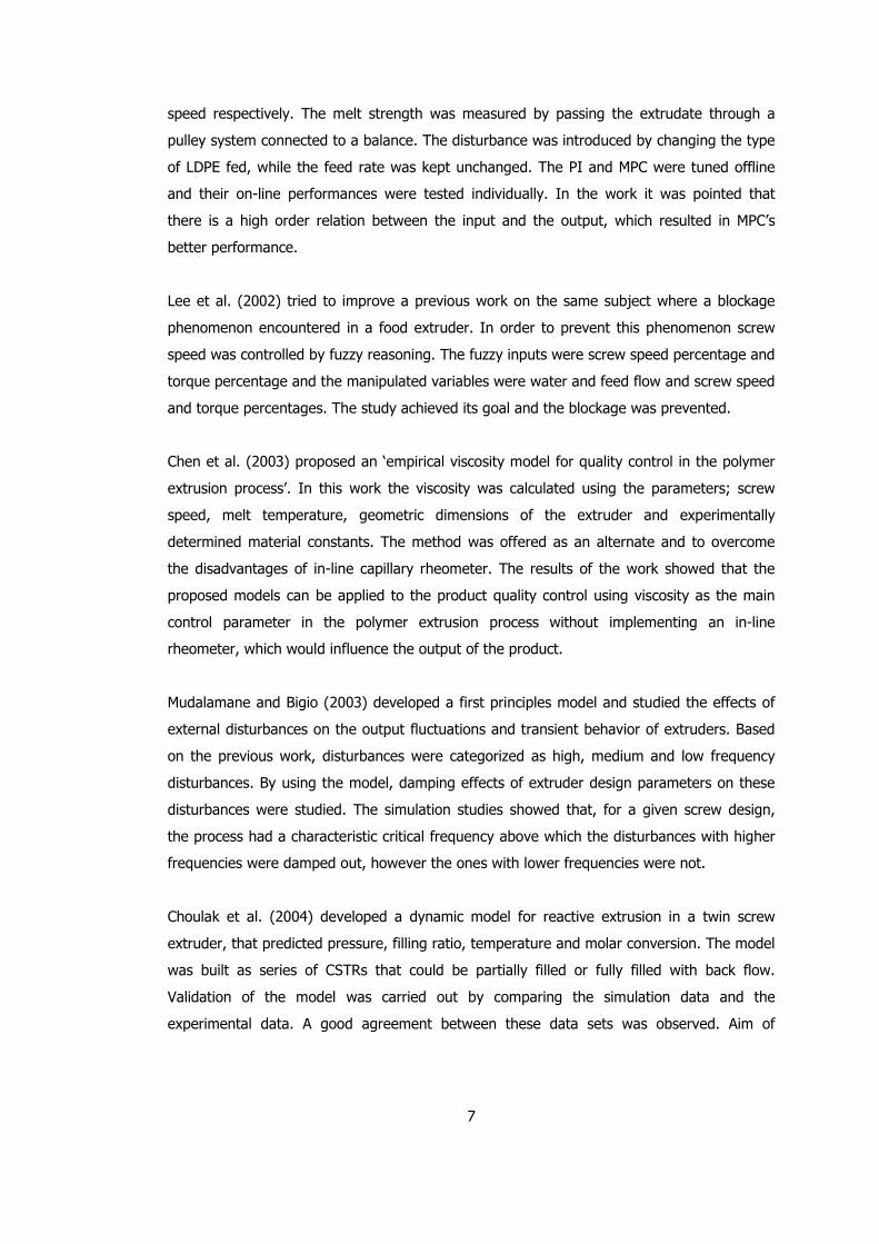
Lee et al. (2002) tried to improve a previous work on the same subject where a blockage
phenomenon encountered in a food extruder. In order to prevent this phenomenon screw
speed was controlled by fuzzy reasoning. The fuzzy inputs were screw speed percentage and
torque percentage and the manipulated variables were water and feed flow and screw speed
and torque percentages. The study achieved its goal and the blockage was prevented.
Chen et al. (2003) proposed an ‘empirical viscosity model for quality control in the polymer
extrusion process’. In this work the viscosity was calculated using the parameters; screw
speed, melt temperature, geometric dimensions of the extruder and experimentally
determined material constants. The method was offered as an alternate and to overcome
the disadvantages of in-line capillary rheometer. The results of the work showed that the
proposed models can be applied to the product quality control using viscosity as the main
control parameter in the polymer extrusion process without implementing an in-line
rheometer, which would influence the output of the product.
Mudalamane and Bigio (2003) developed a first principles model and studied the effects of
external disturbances on the output fluctuations and transient behavior of extruders. Based
on the previous work, disturbances were categorized as high, medium and low frequency
disturbances. By using the model, damping effects of extruder design parameters on these
disturbances were studied. The simulation studies showed that, for a given screw design,
the process had a characteristic critical frequency above which the disturbances with higher
frequencies were damped out, however the ones with lower frequencies were not.
Choulak et al. (2004) developed a dynamic model for reactive extrusion in a twin screw
extruder, that predicted pressure, filling ratio, temperature and molar conversion. The model
was built as series of CSTRs that could be partially filled or fully filled with back flow.
Validation of the model was carried out by comparing the simulation data and the
experimental data. A good agreement between these data sets was observed. Aim of
8
automatic control of polymerization conditions in a twin screw extruder was mentioned but
no control studies were carried out.
Wang et al. (2004) presented a ‘three-stage approach to system identification in the
continuous time’. The three stages are; data acquisition using relay feedback, non-
parametric identification of the system step response, and parametric model fitting of the
identified step response. In the work discrete time noise model was integrated into
continuous time system identification. Experimental results were obtained by applying the
proposed method on a pilot scale food extruder and the results were presented in
comparison with model data.
Previdi et al. (2006) experimentally tested a prototype feedback control system for the
control of volumetric flow in a single screw extruder. The manipulated variables were the
barrel temperatures and die pressure. The work presents all the steps of the controller from
modeling to experimental testing. The results of the tests showed that the control scheme
responded well to disturbance rejections with small offsets on temperature and pressure.
2.2 PET Recycling and PET Degradation
Tanrattanakul et al. (1996) studied ‘toughening of PET by blending with a functionalized
polystyrene-poly(ethylene-co-butylene)-polystyrene (SEBS) block copolymer’. The aim was
to increase fracture strain that was affected by both blend composition and degradation
caused by process conditions. The processes utilized were extrusion and injection molding.
The intrinsic viscosity of PET was measured by Ubbelohde type viscometer using 60w/40w
phenol/tetracholoroethane as solvent. Results shoved that the blending increased the
fracture strain of PET. Torres et al. (2001) also made a similar study. They tried to improve
the thermal and mechanical properties of PET and recycled PET using chain extenders. They
also used the same solvent and equipment type for solution viscosity measurements.
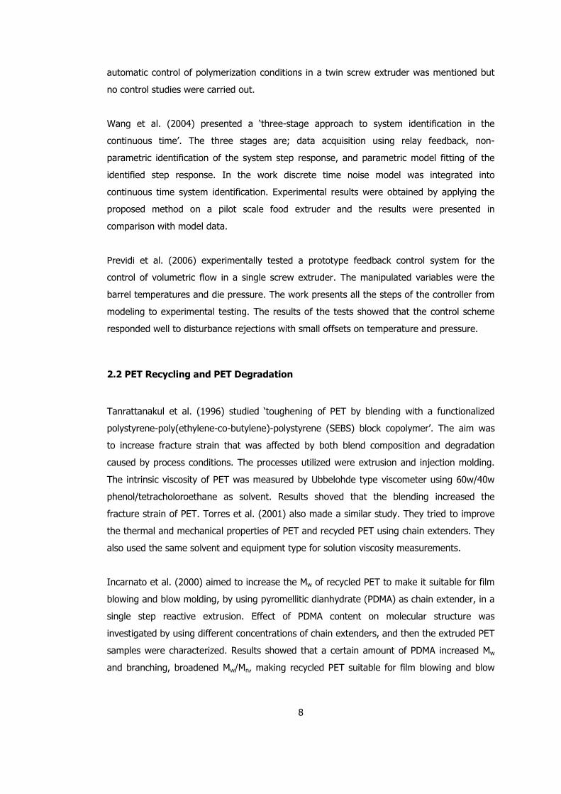
Incarnato et al. (2000) aimed to increase the Mw of recycled PET to make it suitable for film
blowing and blow molding, by using pyromellitic dianhydrate (PDMA) as chain extender, in a
single step reactive extrusion. Effect of PDMA content on molecular structure was
investigated by using different concentrations of chain extenders, and then the extruded PET
samples were characterized. Results showed that a certain amount of PDMA increased Mw
and branching, broadened Mw/Mn, making recycled PET suitable for film blowing and blow
9
molding. Awaja and Davier (2004) made a similar study on an industrial scale extruder,
where PET was recycled by PDMA chain extender. In this work, effects of residence time and
temperature were also studied.
Pawlak et al. (2000) made a study on the ‘characterization of scrap PET’ in order to find
methods of characterization of recycled polymers and to show ‘general tendencies in
property change’. Applied techniques to achieve this goal were; differential scanning
calorimetry (DSC), Fourier transform infrared spectroscopy (FTIR), thermogravimetry (TGA),
dilute solution viscometry and dynamic viscosity measurement via capillary die. In the work,
it was pointed out that the main problem in polymer recycling was the segregation, which
was caused by the impurities that catalysis hydrolysis. In the study, scrap PET from
beverage bottles were obtained from different sources, and extruded in a laboratory scale
single screw extruder. Results showed that the presence of more than 50 ppm PVC made
PET unsuitable for more advanced processes such as film blowing.
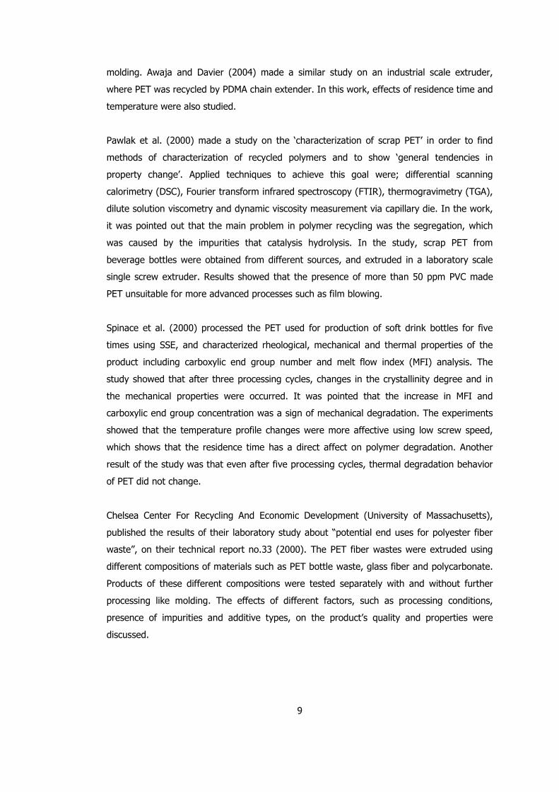
Spinace et al. (2000) processed the PET used for production of soft drink bottles for five
times using SSE, and characterized rheological, mechanical and thermal properties of the
product including carboxylic end group number and melt flow index (MFI) analysis. The
study showed that after three processing cycles, changes in the crystallinity degree and in
the mechanical properties were occurred. It was pointed that the increase in MFI and
carboxylic end group concentration was a sign of mechanical degradation. The experiments
showed that the temperature profile changes were more affective using low screw speed,
which shows that the residence time has a direct affect on polymer degradation. Another
result of the study was that even after five processing cycles, thermal degradation behavior
of PET did not change.
Chelsea Center For Recycling And Economic Development (University of Massachusetts),
published the results of their laboratory study about “potential end uses for polyester fiber
waste”, on their technical report no.33 (2000). The PET fiber wastes were extruded using
different compositions of materials such as PET bottle waste, glass fiber and polycarbonate.
Products of these different compositions were tested separately with and without further
processing like molding. The effects of different factors, such as processing conditions,
presence of impurities and additive types, on the product’s quality and properties were
discussed.
10
Oromiehie and Mamizadeh (2004) studied PET beverage bottle recycling and methods to
improve its properties. The aim was to process and modify the mixture of virgin and recycled
grade PETs, with and without chain extender (PP-graft-MA) by different extrusion methods
and then to characterize the samples. Determination of tensile and thermal properties,
viscosity and Mw, and impact tests were carried out. Results showed that the intrinsic
viscosity ([η]) decreased as thermal process cycles and amount of recycled PET
concentration increased. Also, the chain extender improved the properties of the blends.
Assadi et al. (2004) studied the degradation types of PET during recycling by extrusion. The
experiments were performed using scraps of post-consumer PET, in a single screw extruder
at different temperatures. The Mw of the extruded samples were determined using steric
exclusion chrotomography (SEC), rheological tests and infrared measurements (IR). The
experiments were carried out using nitrogen and air environments with different air
pressures. A kinetic model for PET degradation was built, and results obtained from the
model were compared with the experimental ones. This comparison showed that model
results were in good match for nitrogen and oxygen environments.
Ajawa and Pawel (2005) made a brief review of PET recycling, taking the subject starting
from the synthesis of virgin PET, its properties, processing and applications. Use of chain
extenders was discussed, with the available machinery such as extruders to overcome the
molecular weight loss problem during recycling. Finally, to convert the RPET to a valuable
product, processes such as injection stretch blow molding (ISBM), which is a way to produce
PET bottles, were reviewed.
2.3 Model Predictive Control (MPC)
Marchetti et al. (1983) described the basics of a predictive control algorithm that was based
on discrete convolution models. Developed SISO predictive controller was compared to a
PID controller for three process models on simulation levels, and for an experimental
continuous stirred tank heater. Although predictive controller was superior on simulations, a
significant improvement was not observed in the experimental system. However, it was
pointed that the real advantage of predictive controllers was for MIMO cases.
Maurath et al. (1989) discussed the effects of the controller design parameters on closed
loop performance and robustness for an unconstrained SISO linear process. A stability
11
analysis that considers the plant/model mismatch was developed. Effects of design
parameters on controller’s performance were illustrated on several examples.
Brengel and Seider (1989) developed a model predictive algorithm for nonlinear MIMO case.
The control actions were calculated with a multi step predictor by linearizing ODEs. The
proposed algorithm was capable of easily handling of input and output constraints. In
simulation studies, the multi step predictor out performed the single step predictor.
Garcia et al. (1989) published a survey paper about MPC and compared several predictive
controller algorithms such as DMC, MAC and IMC. They pointed that the significant
advantage of MPC was the ‘flexible constraint handling capability’. Applications of MPC on
nonlinear systems were also investigated and concluded that the adjustment of MPC was
easier although it was not more robust than conventional feed-back controllers.
Morningred et al. (1992) developed an adaptive nonlinear controller similar to standard
linear model predictive controller. In the algorithm the number of tuning parameters could
be reduced to one. For the developed algorithm, effects of the modeling errors were shown,
and it was compared to PI, adaptive linear predictive controller and non-adaptive nonlinear
predictive controller, on a CSTR model. Results showed that the controller was
computationally efficient and could perform well even initially designed with modeling errors.
Meziou et al. (1996) used a dynamic CSTR model of an ethylene-propylene-diene
polymerization reactor to simulate the servo and regulatory performance of three input three
output MIMO DMC. Polynomial equations that relate the process’s gains to the magnitude of
the input change were derived, because the amplitude of the change in the input caused
variations in the gains of the process. Simulation results showed that the capability of MIMO
DMC to reduce the off-spec product amount caused by the set point changes and/or
disturbances.
Özkan et al. (2003) controlled the polymerization reaction in a CSTR with the developed MPC
algorithm that different linear models instead of a non-linear model. The objective function
included finite and infinite horizon cost components. The finite component made the system
move towards the desired operating point and the infinite component, having an upper
bound, brought the system to desired steady state operating point. Simulation results
showed that the proposed controller was successful at achieving the control goals.
12
Biagiola et al. (2005) published their case study about ‘use of state estimation for inferential
non-linear MPC’. The proposed non-linear estimator updates the state vector and estimates
the unmeasured disturbances where feed concentration was not measured. In the algorithm
concentration was inferred via temperature measurements. In simulation studies the
proposed non-linear observer non-linear controller structure is found to have good
performance to reject disturbances even in the presence of significant disturbance variations
and noisy measurements.
2.4 Inferential Control
Doyle III (1998) published a review in which inferential control, linear and non-linear
estimation techniques like moving horizon estimation methods or linearization by output
injection were presented and discussed. New theoretical approaches were presented on a
simple chemical reactor example.
Ogawa et al. (1999) built an inferential control scheme to control the melt index (MI) of the
product of a HDPE process. The MI was estimated by using the measurements of feed and
co-catalyst concentration and temperature measurements. The constructed inferential model
was based on a previous work of writers, simplifying it by means of computational burden.
The calculation of the control law was based on the relations of inferential model. The
system showed good regulatory and set point tracking responses on an industrial polyolefin
production.
Wang et al. (2001) implemented an inferential MPC algorithm on a food extruder, where
screw speed was manipulated variable and the bulk density of the product was controlled
variable, in order to control the product quality. The work also demonstrates the building a
continuous time dynamic model based on multi-rate sampled data. Experimental application
of the algorithm showed that the inferential control system maintains the product quality
within the specific ranges.
Bahar et al. (2004) utilized MPC to build an inferential control loop of an industrial multi
component batch distillation column. The MIMO MPC controlled the product compositions in
a feed-back manner, using the estimated values of the product compositions coming from
the artificial neural network (ANN) estimator. The estimator used the temperature
measurements from the selected trays. Simulation results showed that the unconstrained
13
and constrained MPC performances using ANN estimator, could be alternative to the
controller using direct composition values.
2.5 Singular Value Decomposition (SVD)
Klema and Laub (1980) have given a descriptive introduction to the singular value
decomposition (SVD) from the point of view of its computation and potential
applications. They emphasized certain important details of the implementation of
SVD on a digital computer. They also included a number of illustrative examples and
computed solutions, and concluded that singular value analysis forms a fundamental
basis of modern numerical linear algebra.
Rojas et al. (2004) proposed a strategy for the solution of quadratic performance index of
the optimal control law with constraints on inputs. A MIMO system whose Hessian of the
performance index had a large condition number was chosen for the illustration. Sub-optimal
control laws were obtained using SVD on Hessian matrix. Proposed strategy was compared
against MPC. Although the results were similar, proposed strategy held the advantage of
requiring no solution to the quadratic programming problem.
Zheng and Hoo (2004) used SVD technique to reduce the order of a distributed parameter
system (DPS). The system at hand was a tubular reactor, which was modeled as time series
model (infinite order). Order of this dynamic model was reduced to 3rd order in temperature
and 1st order in concentration. This linear model was then used as the plant model in a
quadratic dynamic model based controller (QDMC) and results were illustrated.
Luyben (2006) quantitatively compared the effectiveness of five different criteria for
selecting the temperature control trays in a distillation column. Their effectiveness were
tested on several systems ranging from ideal binary to azeotropic multi-component. Results
showed that among the tested criteria, SVD analysis provides a simple and effective method
for selecting tray locations.
14
CHAPTER III
BACKGROUND INFORMATION ON PET AND CONTROL TECHNIQUES
The detailed information about PET (synthesis, recycling and degradation), control
techniques (MPC and inferential control) and SVD analysis used in the study are given
below.
3.1 Poly(ethylene terephthalate) (PET)
PET is a thermoplastic resin of polyester family. It was patented in 1941 and was
commercially introduced as a textile fiber in 1953. The first PET bottle was patented in 1973.
PET has become a very important packaging material due to its good barrier and mechanical
properties. It makes a good barrier to gas, to alcohol (requires additional treatment) and to
many of the solvents. Furthermore semi-crystalline PET presents good thermal and
mechanical properties such as high melting temperature (approximately 250 oC).
PET can be synthesized by trans-esterification and/or condensation reactions as shown in
Figure 3.1. Depending on its processing conditions, amorphous (transparent) or semi-
crystalline (opaque and white) PET can be obtained.
The bulk synthesis of PET is carried out at 270 to 285 oC, with continuous removal of gas to
pressure below 1 mm Hg. The removal of methanol or water increases the molecular weight
of the polymer. If the methanol or the water were left in the same system, they would cause
a reverse reaction which would cause depolymerization.
15
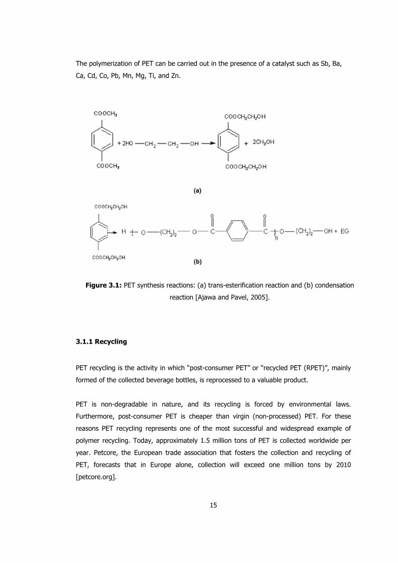
The polymerization of PET can be carried out in the presence of a catalyst such as Sb, Ba,
Ca, Cd, Co, Pb, Mn, Mg, Ti, and Zn.
Figure 3.1: PET synthesis reactions: (a) trans-esterification reaction and (b) condensation
reaction [Ajawa and Pavel, 2005].
3.1.1 Recycling
PET recycling is the activity in which “post-consumer PET” or “recycled PET (RPET)”, mainly
formed of the collected beverage bottles, is reprocessed to a valuable product.
PET is non-degradable in nature, and its recycling is forced by environmental laws.
Furthermore, post-consumer PET is cheaper than virgin (non-processed) PET. For these
reasons PET recycling represents one of the most successful and widespread example of
polymer recycling. Today, approximately 1.5 million tons of PET is collected worldwide per
year. Petcore, the European trade association that fosters the collection and recycling of
PET, forecasts that in Europe alone, collection will exceed one million tons by 2010
[petcore.org].
16
During thermal recycling process, mechanical effects, moisture and presence of impurities
(PVC, adhesives, dyes, etc.), cause the loss of molecular weight (degradation) and lead to a
decrease in intrinsic viscosity ([η]), resulting in decrease in mechanical properties. RPET
having an intrinsic viscosity about 0.60 dl/g would be appropriate for fiber production, 0.65
dl/g for film production, 0.76 dl/g for bottle production and 0.85 dl/g for tire cord production
[Chelsea Center For Recycling And Economic Development, 2000].
RPET should satisfy the specifications given in Table 3.1 to be used as raw material.
Table 3.1: Minimum requirements for RPET flakes to be reprocessed [Ajawa and Pavel,
2005].
Property Value
Intrinsic viscosity ([η]) > 0.7 dl/g
Melting temperature (Tm) > 240 oC.
Water content < 0.02 wt.%
Flake size 0.4 mm < D < 8 mm
Dye content < 10 ppm
Yellowing index < 20
Metal content < 3 ppm
PVC content < 50 ppm
Polyolefin content < 10 ppm
3.1.2 Degradation
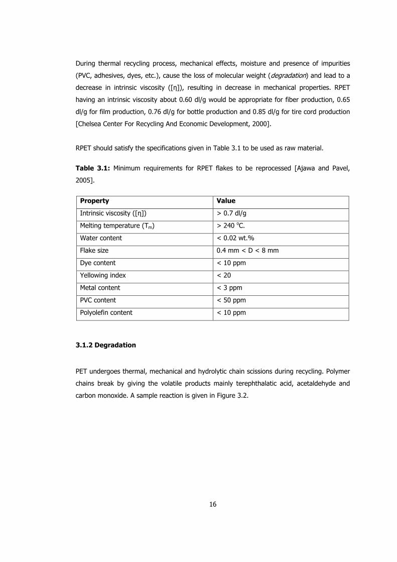
PET undergoes thermal, mechanical and hydrolytic chain scissions during recycling. Polymer
chains break by giving the volatile products mainly terephthalatic acid, acetaldehyde and
carbon monoxide. A sample reaction is given in Figure 3.2.
17
C O
O
H2C
H2C O C
O
C OH
O
+ H2C CH
O C
O
∆
Figure 3.2: Thermal degradation of PET [Karayannidis et al., 2000].
Mechanical degradation occurs due to the physical effects such as shear stress applied by
the extruder screws.
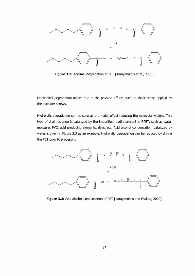
Hydrolytic degradation can be seen as the major effect reducing the molecular weight. This
type of chain scission is catalyzed by the impurities readily present in RPET, such as water
moisture, PVC, acid producing elements, dyes, etc. Acid alcohol condensation, catalyzed by
water is given in Figure 3.3 as an example. Hydrolytic degradation can be reduced by drying
the PET prior to processing.
Figure 3.3: Acid alcohol condensation of PET [Karayannidis and Psalida, 2000].
18
3.2 Control Techniques
In the control of the extruder system (see Chapter 4) MPC and PID techniques using
inferential models are used. A summary on MPC control technique and inferential control will
be given below.
3.2.1 MPC
Beginning from the late 1970’s predictive control techniques such as ‘Model Algorithmic
Control (MAC)’ [Richlet et al., 1978] (also known as Model Predictive Heuristic Control or
MPHC) or ‘Dynamic Matrix Control (DMC)’ [Cutler and Ramaker, 1980] began to gain
importance with the improving computer technology. Up to now, predictive control
techniques proved their efficiencies in many applications.
Although different MPC algorithms utilize different computation techniques, all utilize the
previous knowledge about plant dynamics (plant model) to predict what the plant output will
be after a definite time (prediction horizon), and calculates the next n number of control
actions (control horizon) in an optimal manner.
3.2.1.1 MPC Algorithm
Time
y
yM = aM
y1= a1
y2 = a2
y3 = a3
y4 = a4
h4
h2
h1
h3
4∆t 3∆t 2∆t ∆t 0
Steady state
M∆t
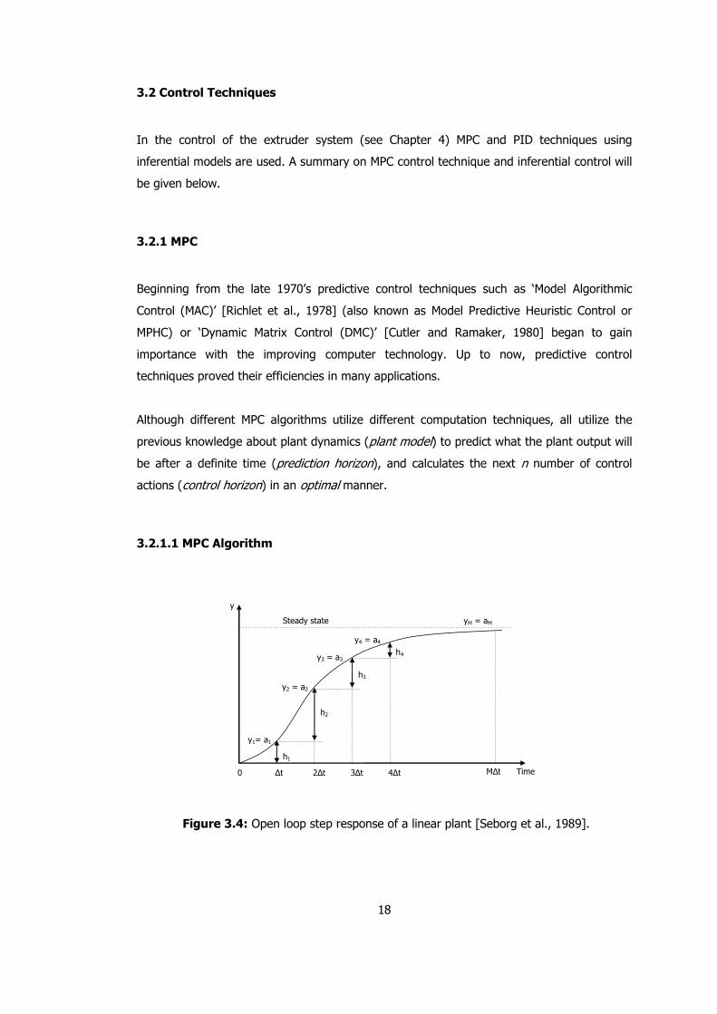
Figure 3.4: Open loop step response of a linear plant [Seborg et al., 1989].
19
In the MPC algorithm, future projection of the plant is calculated using the step response
coefficients (see Figure 3.4) in Equation 3.1 [Marchetti, 1981].
pTp ÊmAE +∆−=
−−
−−
−−
+
∆
∆
∆
−=
−
−
−
−+
+
++
++
++
Rn
R
n
n
Rn
n
nR
c
Rn
d
Rn
c
n
d
n
c
n
d
n
PE
PE
PE
m
m
m
a
a
a
aaa
yy
yy
yy
)1(
)1(
)1(
000
02
2
1
1
1
1
1
2
1
21
22
11
α
α
α
�����
��
�
�
(3.1)
where subscript R denotes the prediction horizon and n denotes the sampling instant. The
superscript c denotes the corrected prediction and d denotes the desired value. The letters
y, m, a and E are used to represent the plant output, plant input, step response coefficients
and error respectively. The predicted errors, P, are calculated as follows.
Rlk
mhPl
k
N
ki
iknil
,....,2,1,
1 1
=
∆=∑ ∑
= +=
−+ (3.2)
If a perfect match between the predicted and the desired values is wanted (Ep = 0) then,
from Equation 3.1 the control action can simply calculated as,
pT ÊAm 1)(
−=∆ (3.3)
Equation 3.3 gives the control action at present sampling instant by predicting the next R
number of plant output. By applying the first element of ∆M vector and repeating the
procedure at every sampling instant the plant output is kept on desired values. But this
control law does not come out to be satisfactory as it tries to force the output to the desired
value at one sampling instant. To overcome this problem two proposed approaches are
Model Algorithmic Control (MAC) [Mehra et al., 1982; Richalet et al., 1978] and Dynamic
Matrix Control (DMC) [Cutler and Ramaker, 1980].
DMC reduces the dimension of ∆M from R (prediction horizon) to L (control horizon), and
only L number of future control actions are calculated. Thus, Equation 3.1 can be rewritten
as,
pp ÊMAE +∆−= (3.4)
20
A being the RxL “Dynamic Matrix” equal to the first L columns of AT. Optimal solution of
Equation 3.4 is obtained by minimizing the performance index by least squares. The solution
for the control action gives,
pTT ÊAAAM 1)(
−=∆ (3.5)
“One difficulty with the above control law is that if the ATA matrix is ill conditioned it can
result in large changes in the manipulated variable (ringing) or even unstable process”
[Marchetti, 1983]. This problem can be eliminated by introducing “weighting matrices” 1W
and 2W , which limit the manipulated variable moves, to the performance index.
pTPTp ÊWMEWEMJ 21)()( ∆+=∆ (3.6)
which results in the following control law:
pTT ÊWARAWAM 2
1
1 )(−+=∆ (3.7)
Here, again, the first control action is applied and new control law is calculated by observing
the plant output at each step. As only the first control action, nm∆ is applied, the control law
can be reduced to,
pT
nn mm ÊK+= −1 (3.8)
where elements of KT (gain matrix), are the elements of the first row of (ATA)-1AT in
Equation 3.5.
3.2.1.2 Constrained MPC
Up to this point no constraints are taken into account in the calculation of the control law.
However, in most processes, constraints should be imposed to the control actions, due to
the physical limitations and/or safety margins of the plant. Constraints may also be placed to
the plant output in order to prevent high deviations on product quality. When the constraints
are introduced, then the solution of the objective function becomes an optimization problem
in the following form:
21
maxmin
maxmin
max1min
21
:
)()(min
yyy
mmm
mmmm
tosubject
n
n
nn
pTPTp
≤≤
≤≤
∆≤−≤∆
∆+=∆
−
ÊWMEWEMJ
(3.9)
3.2.3 Inferential Control
In order to build a feed-back control algorithm, regardless of the controller type, on-line
measurement of the controlled output(s) is required. However, in quite a large number of
chemical process applications direct on-line measurement of the controlled output is late,
expensive or not available at all, which are the cases that limits the construction of the feed-
back control scheme [Seborg et al., 1989]. Feed-forward control could be utilized in such
cases being limited to the presence of measured disturbances and an appropriate model. For
the cases where neither on-line measurement of output nor unmeasured disturbances is
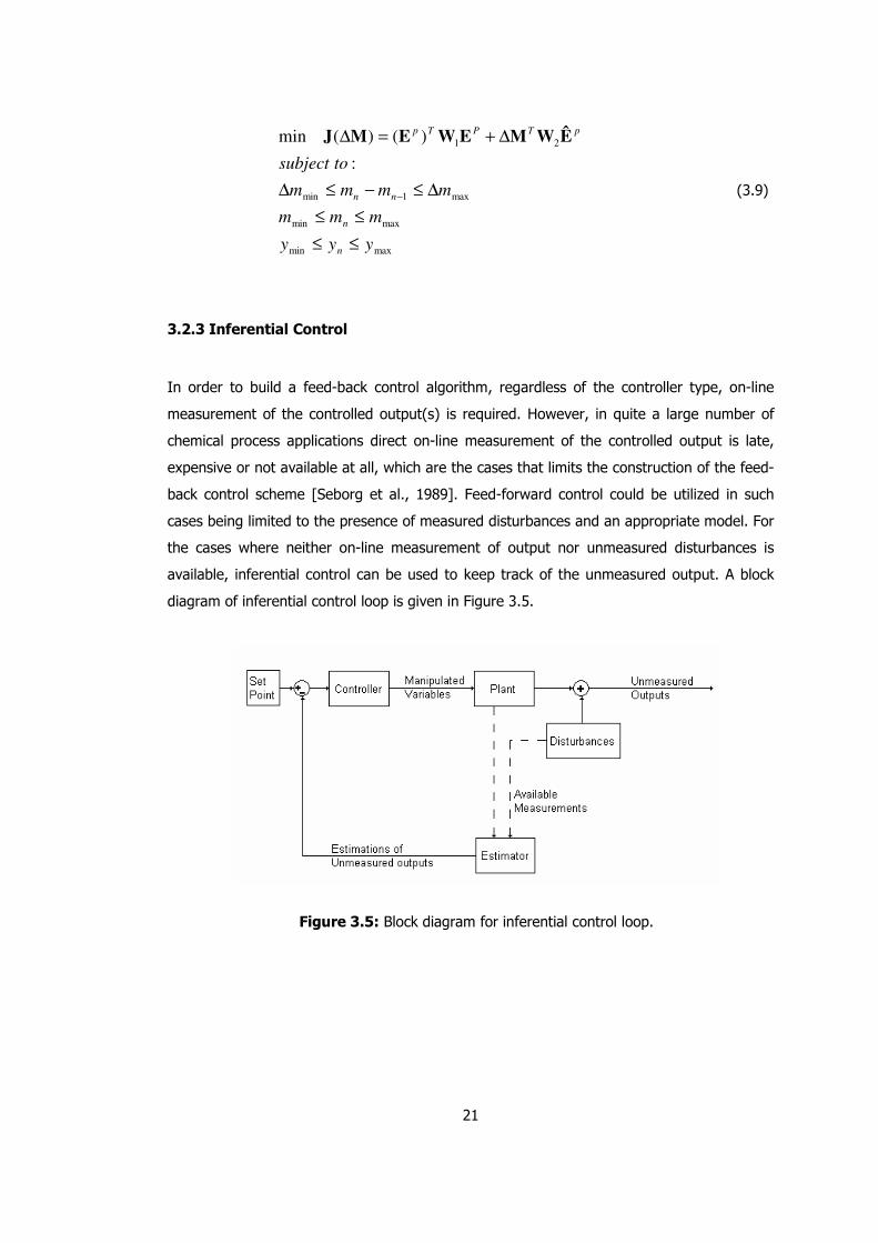
available, inferential control can be used to keep track of the unmeasured output. A block
diagram of inferential control loop is given in Figure 3.5.
Figure 3.5: Block diagram for inferential control loop.
22
3.3 Singular Value Decomposition (SVD)
SVD is an extension of singular value analysis (SVA). It is used to determine the rank and
condition of a matrix and also to determine the strengths and weaknesses of a set of
equations [wikipedia.org]. In control point of view, SVD is utilized for controlled-manipulated
variable pairing for a MIMO system. In the frame of this work, only control aspect of SVD
will be given.
In the simplest form, SVD is the factorization of a rectangular matrix, as follows:
TVUK Σ= (3.10)
Where K is the mxn matrix, U is the nxm orthonormal matrix called left singular matrix
that contains output basis vector directions forK ,Σ is an nxm diagonal matrix of singular
values that can be thought as scalar gains, and V is an mxm orthonormal matrix called
right singular matrix that contains input basis vector directions for K .
Steady state relations of a MIMO system, with n number of outputs and m number of inputs,
can be expressed in vector-matrix form as:
GMY = (3.11)
Where, Y is the output vector, G is the steady state gain matrix and M is the input vector.
It is possible to find which output is sensitive to which input by applying SVD toG . From the
resulting U andV matrices, largest element of 1st column of U ( ny∆ ) is most sensitive to
the changes in the largest element of 1st column of V ( mm ), largest element of 2nd column
of U to the largest element of 2nd column ofV , etc.
For the cases where number of inputs and outputs of the system are not equal to each
other, the pairings corresponding to the zero elements of Σ does not have to be calculated.
Such a calculation is called as the compact SVD.
Another aspect of SVD is the Condition Number, CN. It is defined as the ratio of the largest
and the smallest non-zero singular values:

23
r
lCNσ
σ= (3.12)
For a large CN of G, the system is said to be ill-conditioned. Furthermore, if G is singular,
then it is ill-conditioned.
24
CHAPTER IV
EXPERIMENTAL STUDIES
In the experimental studies done, RPET is extruded at different processing conditions and
samples are collected for molecular weight determination to obtain degradation data.
Materials used, experimental procedure, setup and machinery are presented in this chapter.
4.1 Properties of RPET and Trifluoroacetic Acid (TFA)
RPET is used in the form of flakes in the experiments. The properties of the RPET as
specified by the supplier (AdvanSA, Adana) are presented in Table 4.1.
Two commonly used solvents for PET are, 40wt% tetracholoro ethane – 60wt% phenol
mixture and trifluoroacetic acid (TFA). Being carcinogenic, the first one is eliminated and
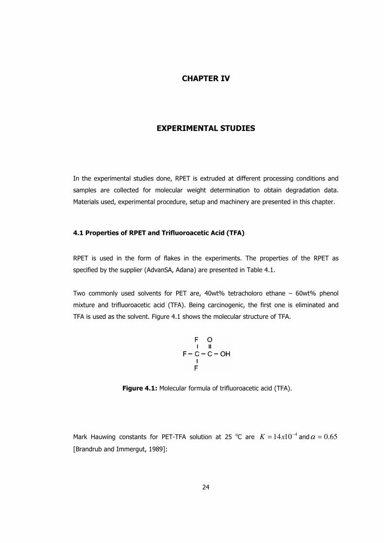
TFA is used as the solvent. Figure 4.1 shows the molecular structure of TFA.
Figure 4.1: Molecular formula of trifluoroacetic acid (TFA).
Mark Hauwing constants for PET-TFA solution at 25 oC are 41014
−= xK and 65.0=α
[Brandrub and Immergut, 1989]:
25
Table 4.1: Properties of RPET resin (AdvanSA)
PVC 60
Polyethylene 5
Metal pieces 0
Adhesive 10
Contaminants (ppm)
Paper pieces 3
Value L, Shining 66.1
Value B, Yellowness 2.6 Lighting Characteristics
Value A, Redness -2.0
Intrinsic Viscosity ([η]) 0.750 dl/g
Glass Transition Temperature (Tg) 60 ºC Material Properties
Melting Temperature (Tm) 255 ºC – 260 ºC
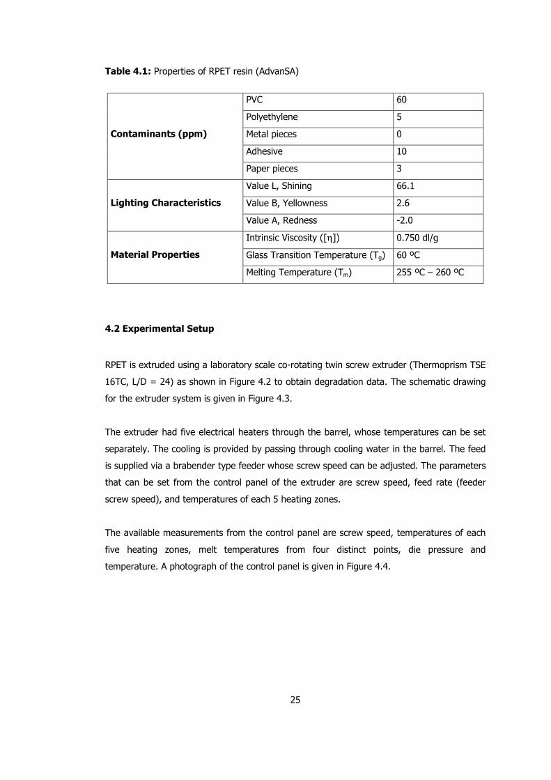
4.2 Experimental Setup
RPET is extruded using a laboratory scale co-rotating twin screw extruder (Thermoprism TSE
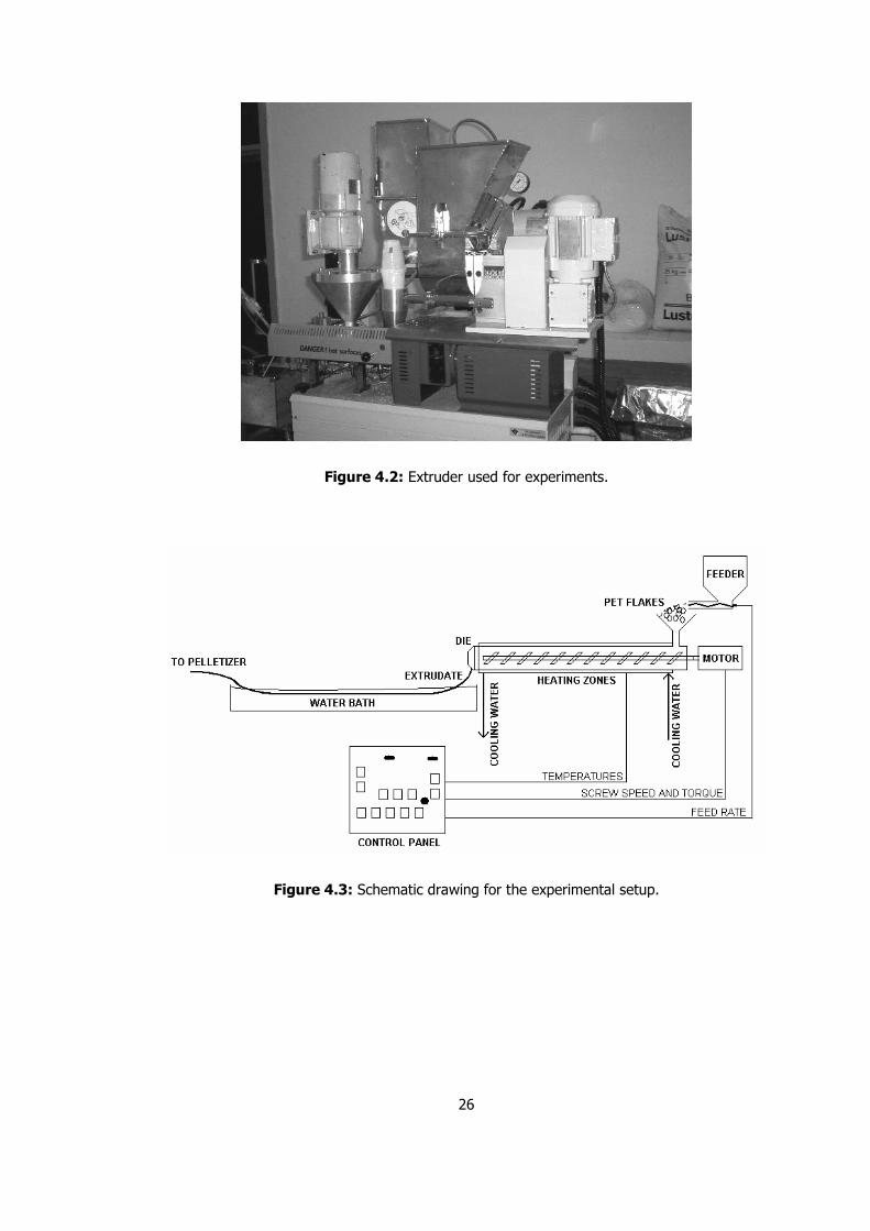
16TC, L/D = 24) as shown in Figure 4.2 to obtain degradation data. The schematic drawing
for the extruder system is given in Figure 4.3.
The extruder had five electrical heaters through the barrel, whose temperatures can be set
separately. The cooling is provided by passing through cooling water in the barrel. The feed
is supplied via a brabender type feeder whose screw speed can be adjusted. The parameters
that can be set from the control panel of the extruder are screw speed, feed rate (feeder
screw speed), and temperatures of each 5 heating zones.
The available measurements from the control panel are screw speed, temperatures of each
five heating zones, melt temperatures from four distinct points, die pressure and
temperature. A photograph of the control panel is given in Figure 4.4.
26
Figure 4.2: Extruder used for experiments.
Figure 4.3: Schematic drawing for the experimental setup.
27
Figure 4.4: Control panel of the extruder (a: die temperature and pressure, b: melt
temperatures, c: barrel temperatures, d: screw speed and torque, e: main feed rate).
4.3 Experimental Procedure
The experiments are carried out in two phases. In the first phase preliminary and steady
state experiments are done and in the second phase dynamic experiments are carried out.
4.3.1 Preliminary Experiments
In the preliminary experiments the effect of temperature on viscosity and molecular weight
is investigated. Also the calibration of the extruder is done.
Effect of Temperature: The effect of temperature on RPET degradation is studied by
eliminating other parameters. Samples are packed firmly in aluminum foil and are held in oil
bath at 4 different temperatures (270, 280, 290, 300oC) for 1, 3 and 5 minutes. The intrinsic
viscosities ([η]) of these 12 samples are determined by dilute solution viscometry (see
Appendix A).
28
The choice of studied temperature and time ranges are based on the studied temperature
and residence time range of extrusion. The residence time range of the extrusion depends
upon the screw speed in a twin screw extruder (see Appendix B). Thus in these
experiments, effect of screw speed in means of residence time is also included indirectly.
Auto ignition temperature of silicone oil limited the testing of higher temperatures.
Calibration of the Extruder: In order to find the flow rate (g/min) equivalent of feed rate
setting of extruder control panel, the feed flow is collected for one minute intervals and
weighted. Different feed rate settings such as 25, 50, 75 and 100, are used and average
values for flow rates are found by repeating the experiments.
The residence times for the studied screw speeds (50, 125, 200, 275, 350, 425 and 500
rpm) are measured by using carbon-black containing polyethylene (PE) pellets as indicator.
The indicator pellets are dropped manually into the feeding point while the main feed
(RPET) is being fed. The time when the product color (originally semi-transparent or opaque
white) changed from gray to black is recorded as the average residence time (ART).
4.3.2 Steady State Experiments
The aim of these experiments is to determine the intrinsic viscosities ([η]) and
corresponding molecular weights (Mv) of products processed at different operating
conditions.
RPET is extruded at 3 different temperatures1, 270, 290 and 310 oC; 4 different feed rate
settings, 25, 50, 75 and 100; and 7 different screw speeds, 50, 125, 200, 275, 350, 425 and
500 rpm, resulting in 84 samples.
After the system is reached its steady state operating conditions (t >> ART) (see Appendix
B) 25-30 grams of samples are collected from the extruded product. The samples are too
1 The barrel temperatures’ setting is a parameter itself for output properties. In this study, the temperature of each
zone is set constant and equal to each other, to eliminate the effect of this parameter. For example, T = 270 oC
means that all the temperatures along the barrel are set to 270 oC.
29
thin and elastic to be pelletized in the pelletizer, thus they are cut into small pieces at hand
to homogenize. From homogenized sample particles, 0.06 gram is weighed for intrinsic
viscosity ([η]) measurements.
4.3.3 Dynamic Experiments
These experiments are aimed to collect the necessary data to model the dynamic response
of the system output (Mv) to the changes in the process parameters (SS, FR and T). In other
words aim is to find out the pattern that Mv follows from one operating condition to other.
Using the data obtained from steady state experiments, operating conditions are selected as
SS = 100 rpm, FR = 7.12 g/min (feed rate setting = 75) and T = 270 oC, for a product
having an intrinsic viscosity value of [η] = 0.6 dl/g, which is suitable for fiber production
[Chelsea Center For Recycling And Economic Development, 2000].
Thus, step changes given in Table 4.2 are introduced one at a time starting from this
operating point. Each step change is given after bringing the system to the initial steady-
state operating point.
Table 4.2: Step changes given to the process variables.
Variable
Initial steady state
value
Plus
change
Minus
change
Screw speed 100 rpm 25 rpm 50 rpm
Feed rate1 7.12 g/gmol 1.04 g/gmol 1.42 g/gmol
Temperature 270 oC 20 oC 20 oC
For screw speed and feed rate changes, the samples are collected at 10 second intervals,
whereas samples are collected at 20 second intervals for temperature changes. This is
because the system responded to the changes in temperature more slowly. The first sample
1 It should be noted that, for step changes on feed rate, feed rate setting of the control panel are taken as the
basis. Calibration data for the feed rate setting and the material flow rate can be found in Appendix C

30
(sample at t = 0) is collected at the time when the step change is introduced. For every
sampling time, outcoming product is collected for 5 seconds. Then, these samples are
broken into small pieces manually for homogenization and 0.06 gram of each sample is
weighted for intrinsic viscosity measurement.
31
CHAPTER V
RESULTS AND DISCUSSIONS
The results of preliminary experiments for the verification of supplier data for RPET
specifications and the experiments on the effect of temperature on degradation of PET are
given below. These will be followed by the results of experiments on the extruder under
steady-state and transient conditions. The results of simulation and modeling studies will be
introduced with discussions.
5.1 Preliminary Experimental Results
Verification of Supplier’s Data: The intrinsic viscosity ([η]) and viscosity average molecular
weight (Mv) of RPET is measured without processing the RPET samples, in order to check
with the supplier’s data. The results of these experiments are given in Table 5.1.
It is found that the experimentally measured value for [η] = 0.75 and corresponding
molecular weight value, Mv = 18363 g/gmol are in a very good agreement with the
supplier’s data with an error of + 0.001 dl/g in [η] and + 26 g/gmol in Mv.
Effect of Temperature on RPET Degradation: As given in Chapter 4, these experiments are
performed in oil bath where samples of RPET are exposed to temperature in the range of
270 - 300 oC for different time durations. The results in terms of Mv are given in Figure 5.1.
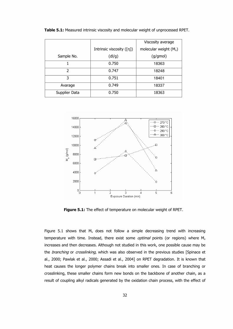
32
Table 5.1: Measured intrinsic viscosity and molecular weight of unprocessed RPET.
Sample No.
Intrinsic viscosity ([η])
(dl/g)
Viscosity average
molecular weight (Mv)
(g/gmol)
1 0.750 18363
2 0.747 18248
3 0.751 18401
Avarage 0.749 18337
Supplier Data 0.750 18363
Figure 5.1: The effect of temperature on molecular weight of RPET.
Figure 5.1 shows that Mv does not follow a simple decreasing trend with increasing
temperature with time. Instead, there exist some optimal points (or regions) where Mv
increases and then decreases. Although not studied in this work, one possible cause may be
the branching or crosslinking, which was also observed in the previous studies [Spinace et
al., 2000; Pawlak et al., 2000; Assadi et al., 2004] on RPET degradation. It is known that
heat causes the longer polymer chains break into smaller ones. In case of branching or
crosslinking, these smaller chains form new bonds on the backbone of another chain, as a
result of coupling alkyl radicals generated by the oxidation chain process, with the effect of
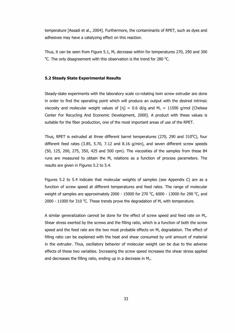
33
temperature [Assadi et al., 2004]. Furthermore, the contaminants of RPET, such as dyes and
adhesives may have a catalyzing effect on this reaction.
Thus, it can be seen from Figure 5.1, Mv decrease within for temperatures 270, 290 and 300 oC. The only disagreement with this observation is the trend for 280 oC.
5.2 Steady State Experimental Results
Steady-state experiments with the laboratory scale co-rotating twin screw extruder are done
in order to find the operating point which will produce an output with the desired intrinsic
viscosity and molecular weight values of [η] = 0.6 dl/g and Mv = 11500 g/mol [Chelsea
Center For Recycling And Economic Development, 2000]. A product with these values is
suitable for the fiber production, one of the most important areas of use of the RPET.
Thus, RPET is extruded at three different barrel temperatures (270, 290 and 310oC), four
different feed rates (3.85, 5.70, 7.12 and 8.16 g/min), and seven different screw speeds
(50, 125, 200, 275, 350, 425 and 500 rpm). The viscosities of the samples from these 84
runs are measured to obtain the Mv relations as a function of process parameters. The
results are given in Figures 5.2 to 5.4.
Figures 5.2 to 5.4 indicate that molecular weights of samples (see Appendix C) are as a
function of screw speed at different temperatures and feed rates. The range of molecular
weight of samples are approximately 2000 - 15000 for 270 oC, 6000 - 13000 for 290 oC, and
2000 - 11000 for 310 oC. These trends prove the degradation of Mv with temperature.
A similar generalization cannot be done for the effect of screw speed and feed rate on Mv.
Shear stress exerted by the screws and the filling ratio, which is a function of both the screw
speed and the feed rate are the two most probable effects on Mv degradation. The effect of
filling ratio can be explained with the heat and shear consumed by unit amount of material
in the extruder. Thus, oscillatory behavior of molecular weight can be due to the adverse
effects of these two variables. Increasing the screw speed increases the shear stress applied
and decreases the filling ratio, ending up in a decrease in Mv.
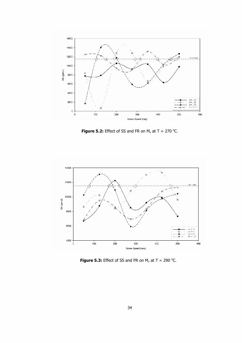
34
Figure 5.2: Effect of SS and FR on Mv at T = 270 oC.
Figure 5.3: Effect of SS and FR on Mv at T = 290 oC.
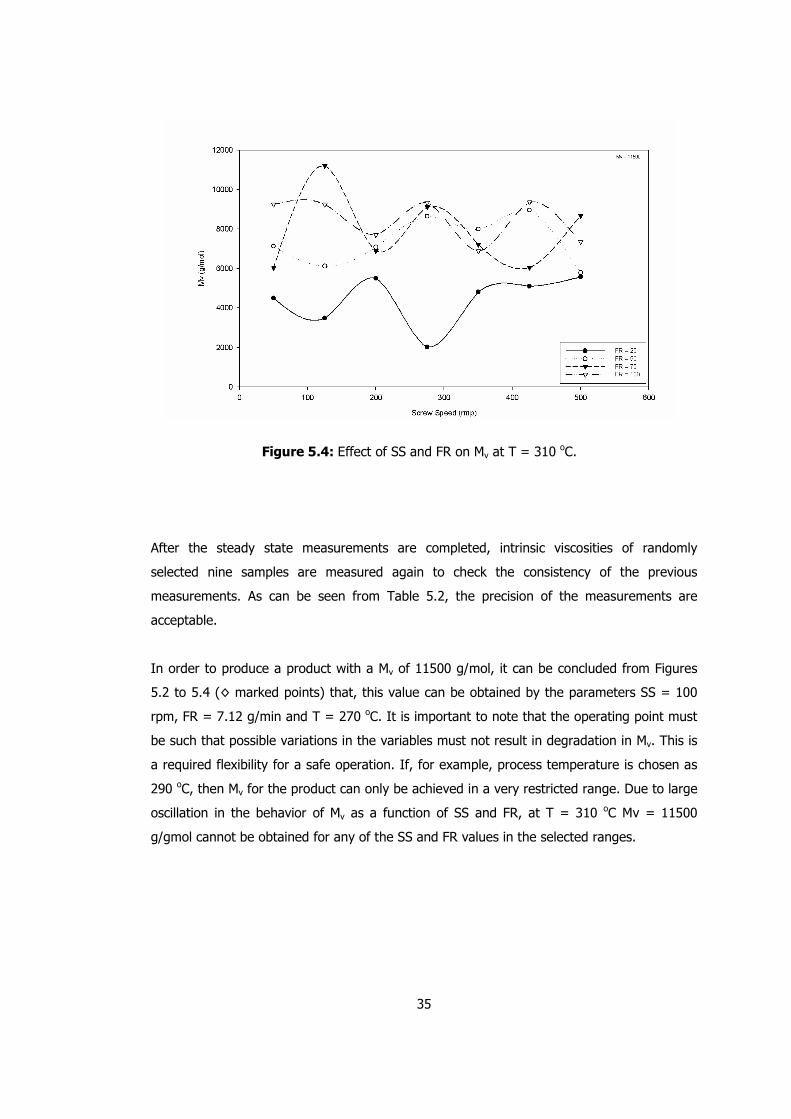
35
Figure 5.4: Effect of SS and FR on Mv at T = 310 oC.
After the steady state measurements are completed, intrinsic viscosities of randomly
selected nine samples are measured again to check the consistency of the previous
measurements. As can be seen from Table 5.2, the precision of the measurements are
acceptable.
In order to produce a product with a Mv of 11500 g/mol, it can be concluded from Figures
5.2 to 5.4 (◊ marked points) that, this value can be obtained by the parameters SS = 100
rpm, FR = 7.12 g/min and T = 270 oC. It is important to note that the operating point must
be such that possible variations in the variables must not result in degradation in Mv. This is
a required flexibility for a safe operation. If, for example, process temperature is chosen as
290 oC, then Mv for the product can only be achieved in a very restricted range. Due to large
oscillation in the behavior of Mv as a function of SS and FR, at T = 310 oC Mv = 11500
g/gmol cannot be obtained for any of the SS and FR values in the selected ranges.
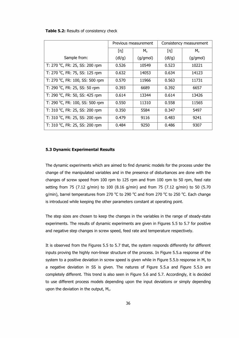
36
Table 5.2: Results of consistency check
Previous measurement Consistency measurement
Sample from:
[η]
(dl/g)
Mv
(g/gmol)
[η]
(dl/g)
Mv
(g/gmol)
T: 270 oC, FR: 25, SS: 200 rpm 0.526 10549 0.523 10221
T: 270 oC, FR: 75, SS: 125 rpm 0.632 14053 0.634 14123
T: 270 oC, FR: 100, SS: 500 rpm 0.570 11966 0.563 11731
T: 290 oC, FR: 25, SS: 50 rpm 0.393 6689 0.392 6657
T: 290 oC, FR: 50, SS: 425 rpm 0.614 13344 0.614 13426
T: 290 oC, FR: 100, SS: 500 rpm 0.550 11310 0.558 11565
T: 310 oC, FR: 25, SS: 200 rpm 0.350 5584 0.347 5497
T: 310 oC, FR: 25, SS: 200 rpm 0.479 9116 0.483 9241
T: 310 oC, FR: 25, SS: 200 rpm 0.484 9250 0.486 9307
5.3 Dynamic Experimental Results
The dynamic experiments which are aimed to find dynamic models for the process under the
change of the manipulated variables and in the presence of disturbances are done with the
changes of screw speed from 100 rpm to 125 rpm and from 100 rpm to 50 rpm, feed rate
setting from 75 (7.12 g/min) to 100 (8.16 g/min) and from 75 (7.12 g/min) to 50 (5.70
g/min), barrel temperatures from 270 oC to 290 oC and from 270 oC to 250 oC. Each change
is introduced while keeping the other parameters constant at operating point.
The step sizes are chosen to keep the changes in the variables in the range of steady-state
experiments. The results of dynamic experiments are given in Figures 5.5 to 5.7 for positive
and negative step changes in screw speed, feed rate and temperature respectively.
It is observed from the Figures 5.5 to 5.7 that, the system responds differently for different
inputs proving the highly non-linear structure of the process. In Figure 5.5.a response of the
system to a positive deviation in screw speed is given while in Figure 5.5.b response in Mv to
a negative deviation in SS is given. The natures of Figure 5.5.a and Figure 5.5.b are
completely different. This trend is also seen in Figure 5.6 and 5.7. Accordingly, it is decided
to use different process models depending upon the input deviations or simply depending
upon the deviation in the output, Mv.
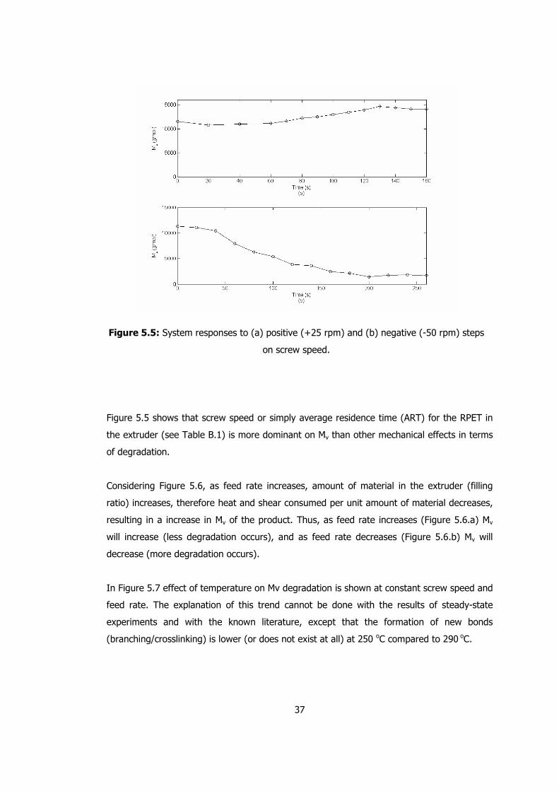
37
Figure 5.5: System responses to (a) positive (+25 rpm) and (b) negative (-50 rpm) steps
on screw speed.
Figure 5.5 shows that screw speed or simply average residence time (ART) for the RPET in
the extruder (see Table B.1) is more dominant on Mv than other mechanical effects in terms
of degradation.
Considering Figure 5.6, as feed rate increases, amount of material in the extruder (filling
ratio) increases, therefore heat and shear consumed per unit amount of material decreases,
resulting in a increase in Mv of the product. Thus, as feed rate increases (Figure 5.6.a) Mv
will increase (less degradation occurs), and as feed rate decreases (Figure 5.6.b) Mv will
decrease (more degradation occurs).
In Figure 5.7 effect of temperature on Mv degradation is shown at constant screw speed and
feed rate. The explanation of this trend cannot be done with the results of steady-state
experiments and with the known literature, except that the formation of new bonds
(branching/crosslinking) is lower (or does not exist at all) at 250 oC compared to 290 oC.
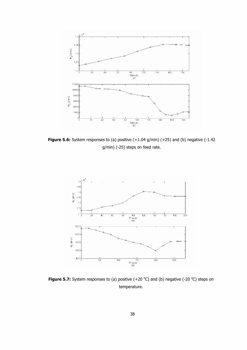
38
Figure 5.6: System responses to (a) positive (+1.04 g/min) (+25) and (b) negative (-1.42
g/min) (-25) steps on feed rate.
Figure 5.7: System responses to (a) positive (+20 oC) and (b) negative (-20 oC) steps on
temperature.
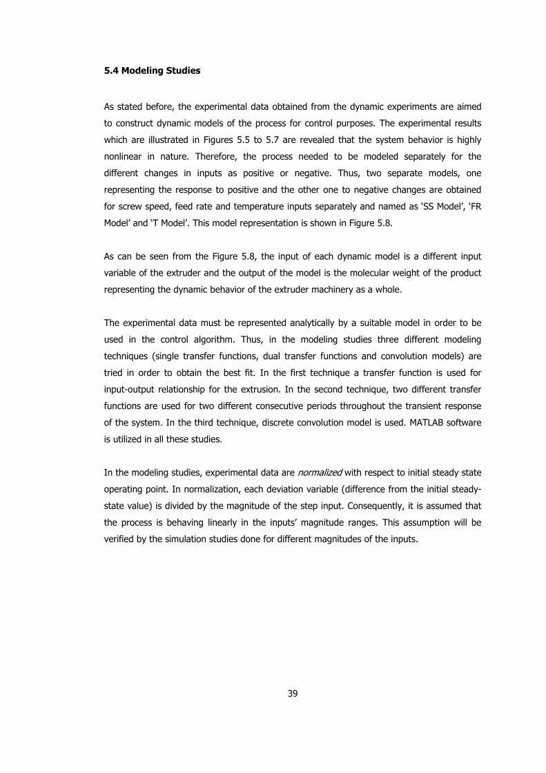
39
5.4 Modeling Studies
As stated before, the experimental data obtained from the dynamic experiments are aimed
to construct dynamic models of the process for control purposes. The experimental results
which are illustrated in Figures 5.5 to 5.7 are revealed that the system behavior is highly
nonlinear in nature. Therefore, the process needed to be modeled separately for the
different changes in inputs as positive or negative. Thus, two separate models, one
representing the response to positive and the other one to negative changes are obtained
for screw speed, feed rate and temperature inputs separately and named as ‘SS Model’, ‘FR
Model’ and ‘T Model’. This model representation is shown in Figure 5.8.
As can be seen from the Figure 5.8, the input of each dynamic model is a different input
variable of the extruder and the output of the model is the molecular weight of the product
representing the dynamic behavior of the extruder machinery as a whole.
The experimental data must be represented analytically by a suitable model in order to be
used in the control algorithm. Thus, in the modeling studies three different modeling
techniques (single transfer functions, dual transfer functions and convolution models) are
tried in order to obtain the best fit. In the first technique a transfer function is used for
input-output relationship for the extrusion. In the second technique, two different transfer
functions are used for two different consecutive periods throughout the transient response
of the system. In the third technique, discrete convolution model is used. MATLAB software
is utilized in all these studies.
In the modeling studies, experimental data are normalized with respect to initial steady state
operating point. In normalization, each deviation variable (difference from the initial steady-
state value) is divided by the magnitude of the step input. Consequently, it is assumed that
the process is behaving linearly in the inputs’ magnitude ranges. This assumption will be
verified by the simulation studies done for different magnitudes of the inputs.
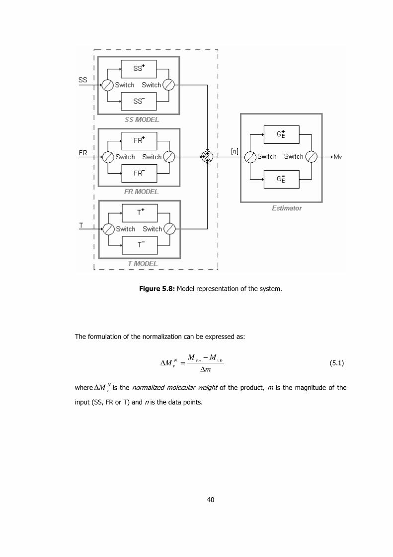
40
Figure 5.8: Model representation of the system.
The formulation of the normalization can be expressed as:
m
MMM
vnvN
v∆
−=∆ 0 (5.1)
where N
vM∆ is the normalized molecular weight of the product, m is the magnitude of the
input (SS, FR or T) and n is the data points.
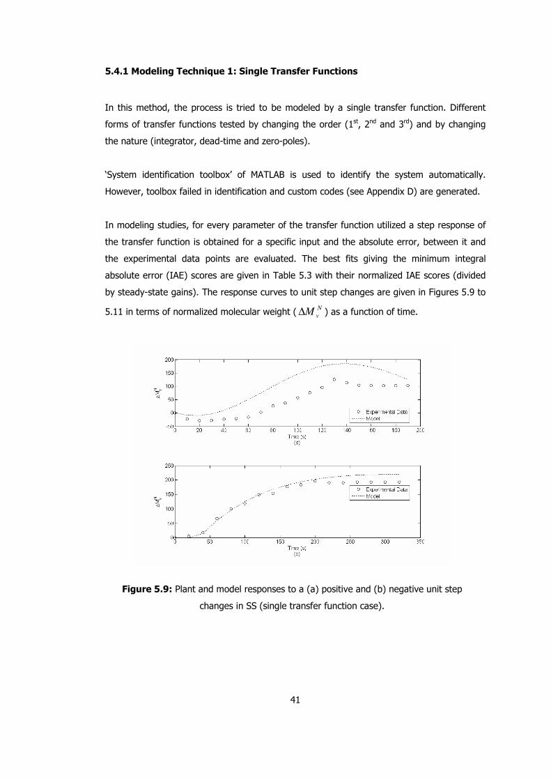
41
5.4.1 Modeling Technique 1: Single Transfer Functions
In this method, the process is tried to be modeled by a single transfer function. Different
forms of transfer functions tested by changing the order (1st, 2nd and 3rd) and by changing
the nature (integrator, dead-time and zero-poles).
‘System identification toolbox’ of MATLAB is used to identify the system automatically.
However, toolbox failed in identification and custom codes (see Appendix D) are generated.
In modeling studies, for every parameter of the transfer function utilized a step response of
the transfer function is obtained for a specific input and the absolute error, between it and
the experimental data points are evaluated. The best fits giving the minimum integral
absolute error (IAE) scores are given in Table 5.3 with their normalized IAE scores (divided
by steady-state gains). The response curves to unit step changes are given in Figures 5.9 to
5.11 in terms of normalized molecular weight ( N
vM∆ ) as a function of time.
Figure 5.9: Plant and model responses to a (a) positive and (b) negative unit step
changes in SS (single transfer function case).
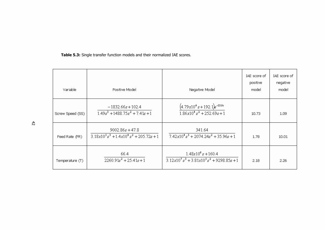
42
Table 5.3: Single transfer function models and their normalized IAE scores.
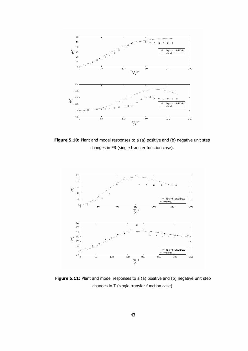
43
Figure 5.10: Plant and model responses to a (a) positive and (b) negative unit step
changes in FR (single transfer function case).
Figure 5.11: Plant and model responses to a (a) positive and (b) negative unit step
changes in T (single transfer function case).
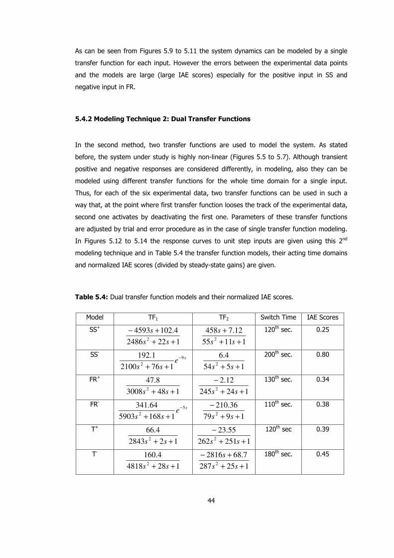
44
As can be seen from Figures 5.9 to 5.11 the system dynamics can be modeled by a single
transfer function for each input. However the errors between the experimental data points
and the models are large (large IAE scores) especially for the positive input in SS and
negative input in FR.
5.4.2 Modeling Technique 2: Dual Transfer Functions
In the second method, two transfer functions are used to model the system. As stated
before, the system under study is highly non-linear (Figures 5.5 to 5.7). Although transient
positive and negative responses are considered differently, in modeling, also they can be
modeled using different transfer functions for the whole time domain for a single input.
Thus, for each of the six experimental data, two transfer functions can be used in such a
way that, at the point where first transfer function looses the track of the experimental data,
second one activates by deactivating the first one. Parameters of these transfer functions
are adjusted by trial and error procedure as in the case of single transfer function modeling.
In Figures 5.12 to 5.14 the response curves to unit step inputs are given using this 2nd
modeling technique and in Table 5.4 the transfer function models, their acting time domains
and normalized IAE scores (divided by steady-state gains) are given.
Table 5.4: Dual transfer function models and their normalized IAE scores.
Model TF1 TF2 Switch Time IAE Scores
SS+
1222486
4.10245932 ++
+−
ss
s
11155
12.74582 ++
+
ss
s
120th sec. 0.25
SS- s
ess
9
21762100
1.192 −
++
1554
4.62 ++ ss
200th sec. 0.80
FR+
1483008
8.472 ++ ss
124245
12.22 ++
−
ss
130th sec. 0.34
FR- s
ess
5
211685903
64.341 −
++
1979
36.2102 ++
−
ss
110th sec. 0.38
T+
122843
4.662 ++ ss
1251262
55.232 ++
−
ss
120th sec 0.39
T-
1284818
4.1602 ++ ss
125287
7.6828162 ++
+−
ss
s
180th sec. 0.45
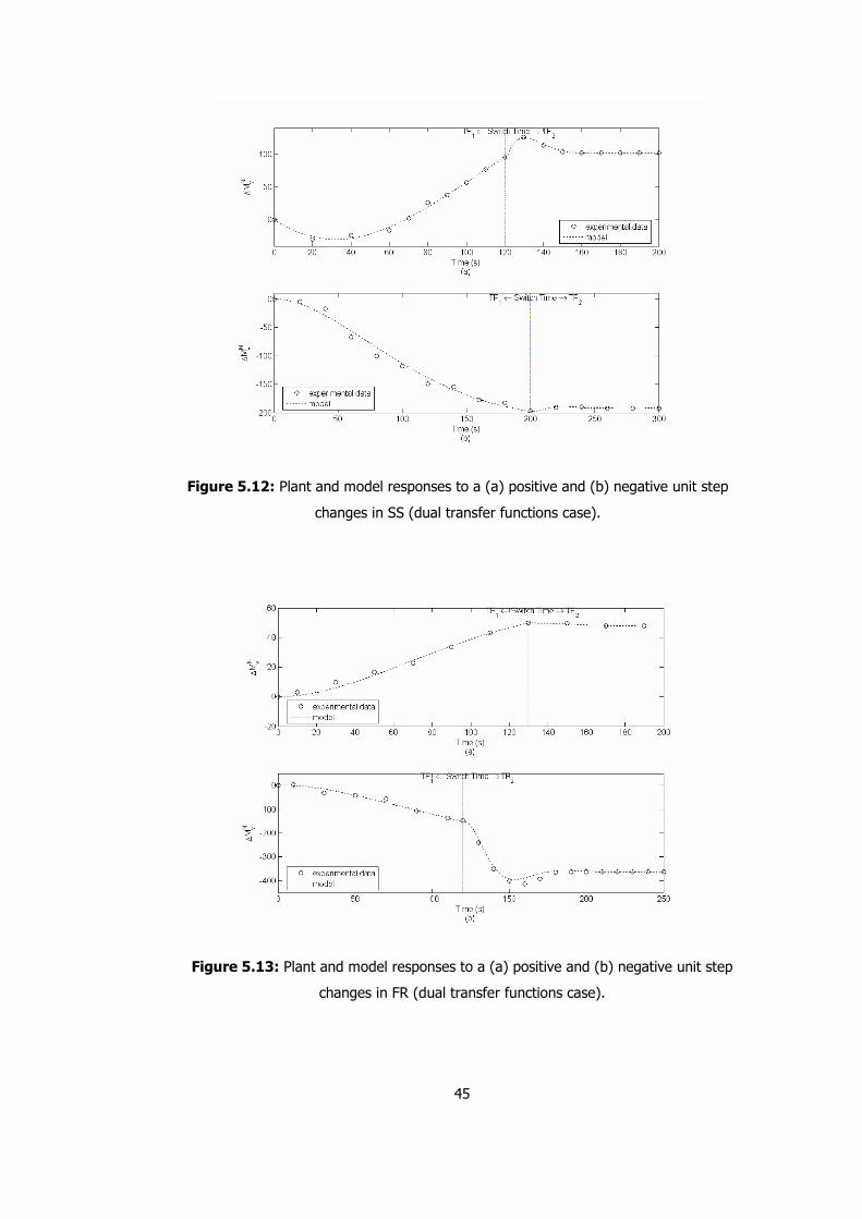
45
Figure 5.12: Plant and model responses to a (a) positive and (b) negative unit step
changes in SS (dual transfer functions case).
Figure 5.13: Plant and model responses to a (a) positive and (b) negative unit step
changes in FR (dual transfer functions case).
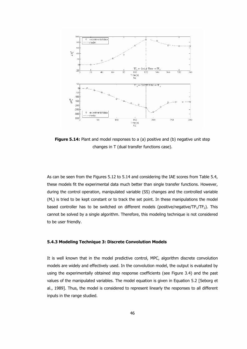
46
Figure 5.14: Plant and model responses to a (a) positive and (b) negative unit step
changes in T (dual transfer functions case).
As can be seen from the Figures 5.12 to 5.14 and considering the IAE scores from Table 5.4,
these models fit the experimental data much better than single transfer functions. However,
during the control operation, manipulated variable (SS) changes and the controlled variable
(Mv) is tried to be kept constant or to track the set point. In these manipulations the model
based controller has to be switched on different models (positive/negative/TF1/TF2). This
cannot be solved by a single algorithm. Therefore, this modeling technique is not considered
to be user friendly.
5.4.3 Modeling Technique 3: Discrete Convolution Models
It is well known that in the model predictive control, MPC, algorithm discrete convolution
models are widely and effectively used. In the convolution model, the output is evaluated by
using the experimentally obtained step response coefficients (see Figure 3.4) and the past
values of the manipulated variables. The model equation is given in Equation 5.2 [Seborg et
al., 1989]. Thus, the model is considered to represent linearly the responses to all different
inputs in the range studied.
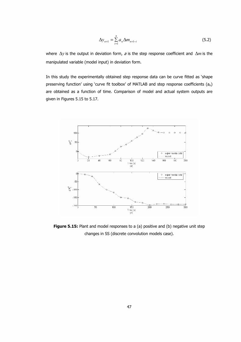
47
inn
n
in may −+
=+ ∆∑=∆ 1
11 (5.2)
where y∆ is the output in deviation form, a is the step response coefficient and m∆ is the
manipulated variable (model input) in deviation form.
In this study the experimentally obtained step response data can be curve fitted as ‘shape
preserving function’ using ‘curve fit toolbox’ of MATLAB and step response coefficients (an)
are obtained as a function of time. Comparison of model and actual system outputs are
given in Figures 5.15 to 5.17.
Figure 5.15: Plant and model responses to a (a) positive and (b) negative unit step
changes in SS (discrete convolution models case).
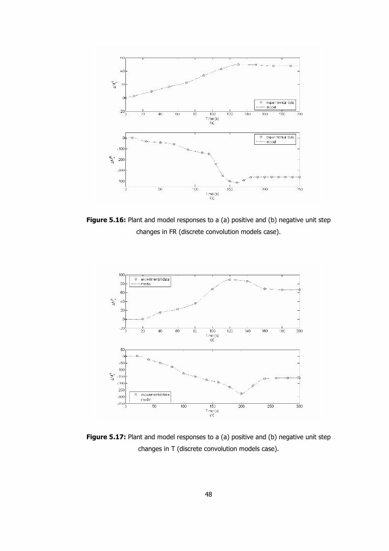
48
Figure 5.16: Plant and model responses to a (a) positive and (b) negative unit step
changes in FR (discrete convolution models case).
Figure 5.17: Plant and model responses to a (a) positive and (b) negative unit step
changes in T (discrete convolution models case).
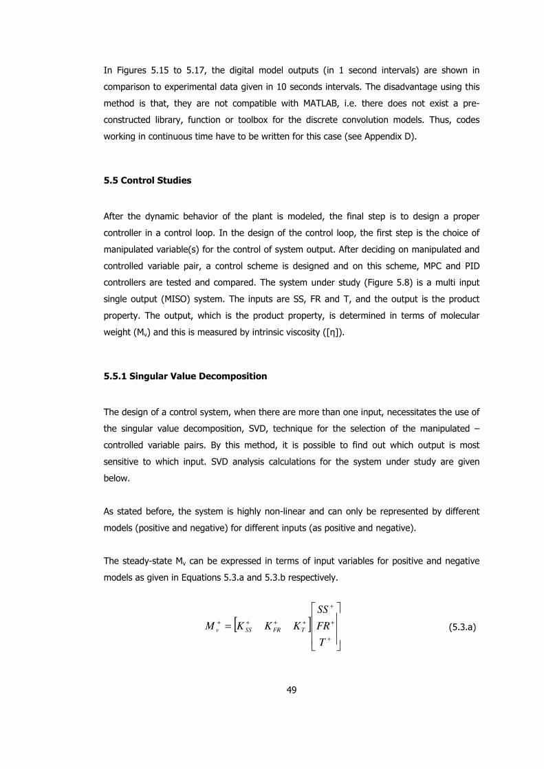
49
In Figures 5.15 to 5.17, the digital model outputs (in 1 second intervals) are shown in
comparison to experimental data given in 10 seconds intervals. The disadvantage using this
method is that, they are not compatible with MATLAB, i.e. there does not exist a pre-
constructed library, function or toolbox for the discrete convolution models. Thus, codes
working in continuous time have to be written for this case (see Appendix D).
5.5 Control Studies
After the dynamic behavior of the plant is modeled, the final step is to design a proper
controller in a control loop. In the design of the control loop, the first step is the choice of
manipulated variable(s) for the control of system output. After deciding on manipulated and
controlled variable pair, a control scheme is designed and on this scheme, MPC and PID
controllers are tested and compared. The system under study (Figure 5.8) is a multi input
single output (MISO) system. The inputs are SS, FR and T, and the output is the product
property. The output, which is the product property, is determined in terms of molecular
weight (Mv) and this is measured by intrinsic viscosity ([η]).
5.5.1 Singular Value Decomposition
The design of a control system, when there are more than one input, necessitates the use of
the singular value decomposition, SVD, technique for the selection of the manipulated –
controlled variable pairs. By this method, it is possible to find out which output is most
sensitive to which input. SVD analysis calculations for the system under study are given
below.
As stated before, the system is highly non-linear and can only be represented by different
models (positive and negative) for different inputs (as positive and negative).
The steady-state Mv can be expressed in terms of input variables for positive and negative
models as given in Equations 5.3.a and 5.3.b respectively.
[ ]
=+
+
+
++++
T
FR
SS
KKKM TFRSSv
(5.3.a)
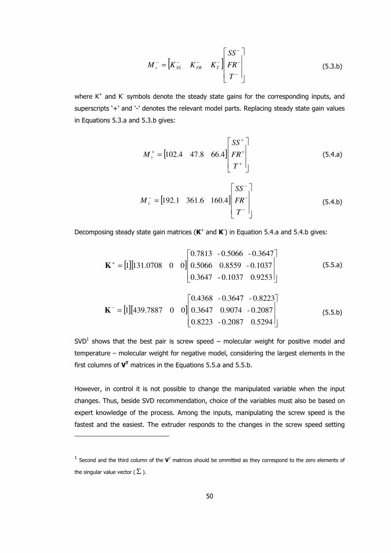
50
[ ]
=−
−
−
−−−−
T
FR
SS
KKKM TFRSSv
(5.3.b)
where K+ and K- symbols denote the steady state gains for the corresponding inputs, and
superscripts ‘+’ and ‘-’ denotes the relevant model parts. Replacing steady state gain values
in Equations 5.3.a and 5.3.b gives:
[ ]
=+
+
+
+
T
FR
SS
M v 4.668.474.102
[ ]
=−
−
−
−
T
FR
SS
M v 4.1606.3611.192
(5.4.a)
(5.4.b)
Decomposing steady state gain matrices (K+ and K-) in Equation 5.4.a and 5.4.b gives:
[ ][ ]
=+
0.9253 0.1037- 0.3647
0.1037- 0.8559 0.5066
0.3647- 0.5066- 0.7813
000708.1311K
[ ][ ]
=−
0.5294 0.2087- 0.8223
0.2087- 0.9074 0.3647
0.8223- 0.3647- 0.4368
00439.78871K
(5.5.a)
(5.5.b)
SVD1 shows that the best pair is screw speed – molecular weight for positive model and
temperature – molecular weight for negative model, considering the largest elements in the
first columns of VT matrices in the Equations 5.5.a and 5.5.b.
However, in control it is not possible to change the manipulated variable when the input
changes. Thus, beside SVD recommendation, choice of the variables must also be based on
expert knowledge of the process. Among the inputs, manipulating the screw speed is the
fastest and the easiest. The extruder responds to the changes in the screw speed setting
1 Second and the third column of the VT matrices should be ommitted as they correspond to the zero elements of
the singular value vector (Σ ).
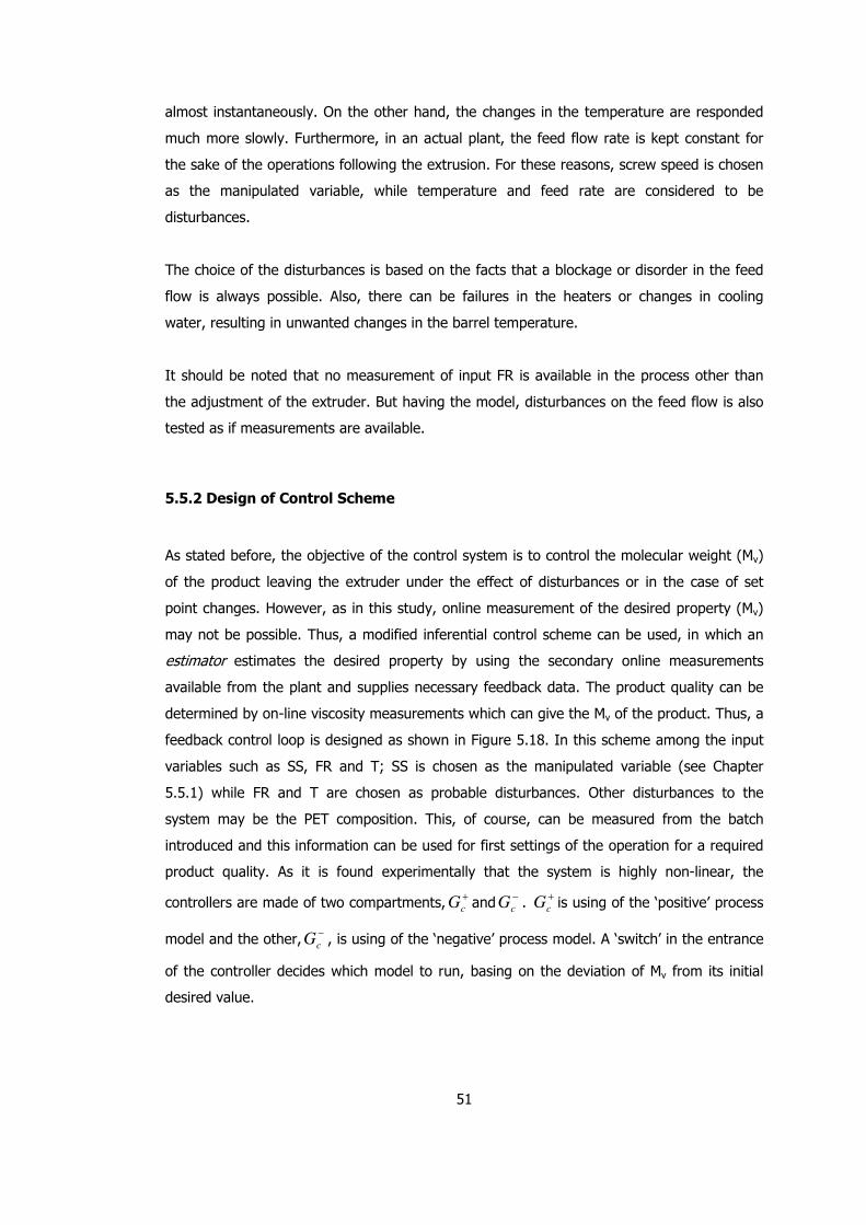
51
almost instantaneously. On the other hand, the changes in the temperature are responded
much more slowly. Furthermore, in an actual plant, the feed flow rate is kept constant for
the sake of the operations following the extrusion. For these reasons, screw speed is chosen
as the manipulated variable, while temperature and feed rate are considered to be
disturbances.
The choice of the disturbances is based on the facts that a blockage or disorder in the feed
flow is always possible. Also, there can be failures in the heaters or changes in cooling
water, resulting in unwanted changes in the barrel temperature.
It should be noted that no measurement of input FR is available in the process other than
the adjustment of the extruder. But having the model, disturbances on the feed flow is also
tested as if measurements are available.
5.5.2 Design of Control Scheme
As stated before, the objective of the control system is to control the molecular weight (Mv)
of the product leaving the extruder under the effect of disturbances or in the case of set
point changes. However, as in this study, online measurement of the desired property (Mv)
may not be possible. Thus, a modified inferential control scheme can be used, in which an
estimator estimates the desired property by using the secondary online measurements
available from the plant and supplies necessary feedback data. The product quality can be
determined by on-line viscosity measurements which can give the Mv of the product. Thus, a
feedback control loop is designed as shown in Figure 5.18. In this scheme among the input
variables such as SS, FR and T; SS is chosen as the manipulated variable (see Chapter
5.5.1) while FR and T are chosen as probable disturbances. Other disturbances to the
system may be the PET composition. This, of course, can be measured from the batch
introduced and this information can be used for first settings of the operation for a required
product quality. As it is found experimentally that the system is highly non-linear, the
controllers are made of two compartments, +cG and −
cG . +cG is using of the ‘positive’ process
model and the other, −cG , is using of the ‘negative’ process model. A ‘switch’ in the entrance
of the controller decides which model to run, basing on the deviation of Mv from its initial
desired value.
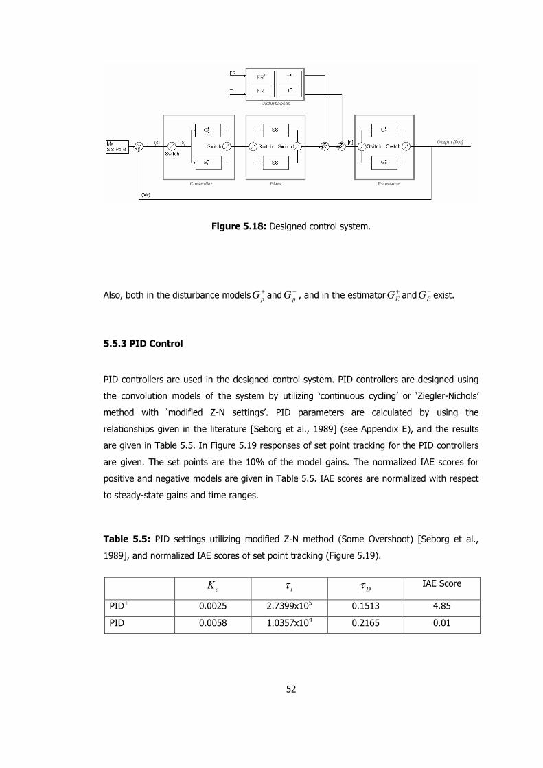
52
Figure 5.18: Designed control system.
Also, both in the disturbance models +pG and −
pG , and in the estimator +EG and −
EG exist.
5.5.3 PID Control
PID controllers are used in the designed control system. PID controllers are designed using
the convolution models of the system by utilizing ‘continuous cycling’ or ‘Ziegler-Nichols’
method with ‘modified Z-N settings’. PID parameters are calculated by using the
relationships given in the literature [Seborg et al., 1989] (see Appendix E), and the results
are given in Table 5.5. In Figure 5.19 responses of set point tracking for the PID controllers
are given. The set points are the 10% of the model gains. The normalized IAE scores for
positive and negative models are given in Table 5.5. IAE scores are normalized with respect
to steady-state gains and time ranges.
Table 5.5: PID settings utilizing modified Z-N method (Some Overshoot) [Seborg et al.,
1989], and normalized IAE scores of set point tracking (Figure 5.19).
cK iτ Dτ IAE Score
PID+ 0.0025 2.7399x10⁵ 0.1513 4.85
PID- 0.0058 1.0357x10⁴ 0.2165 0.01
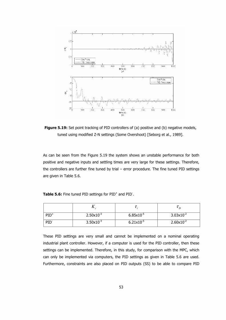
53
Figure 5.19: Set point tracking of PID controllers of (a) positive and (b) negative models,
tuned using modified Z-N settings (Some Overshoot) [Seborg et al., 1989].
As can be seen from the Figure 5.19 the system shows an unstable performance for both
positive and negative inputs and settling times are very large for these settings. Therefore,
the controllers are further fine tuned by trial – error procedure. The fine tuned PID settings
are given in Table 5.6.
Table 5.6: Fine tuned PID settings for PID+ and PID-.
cK iτ Dτ
PID+ 2.50x10⁻³ 6.85x10⁻⁵ 3.03x10⁻²
PID- 3.50x10⁻³ 6.21x10⁻⁵ 2.60x10⁻²
These PID settings are very small and cannot be implemented on a nominal operating
industrial plant controller. However, if a computer is used for the PID controller, then these
settings can be implemented. Therefore, in this study, for comparison with the MPC, which
can only be implemented via computers, the PID settings as given in Table 5.6 are used.
Furthermore, constraints are also placed on PID outputs (SS) to be able to compare PID
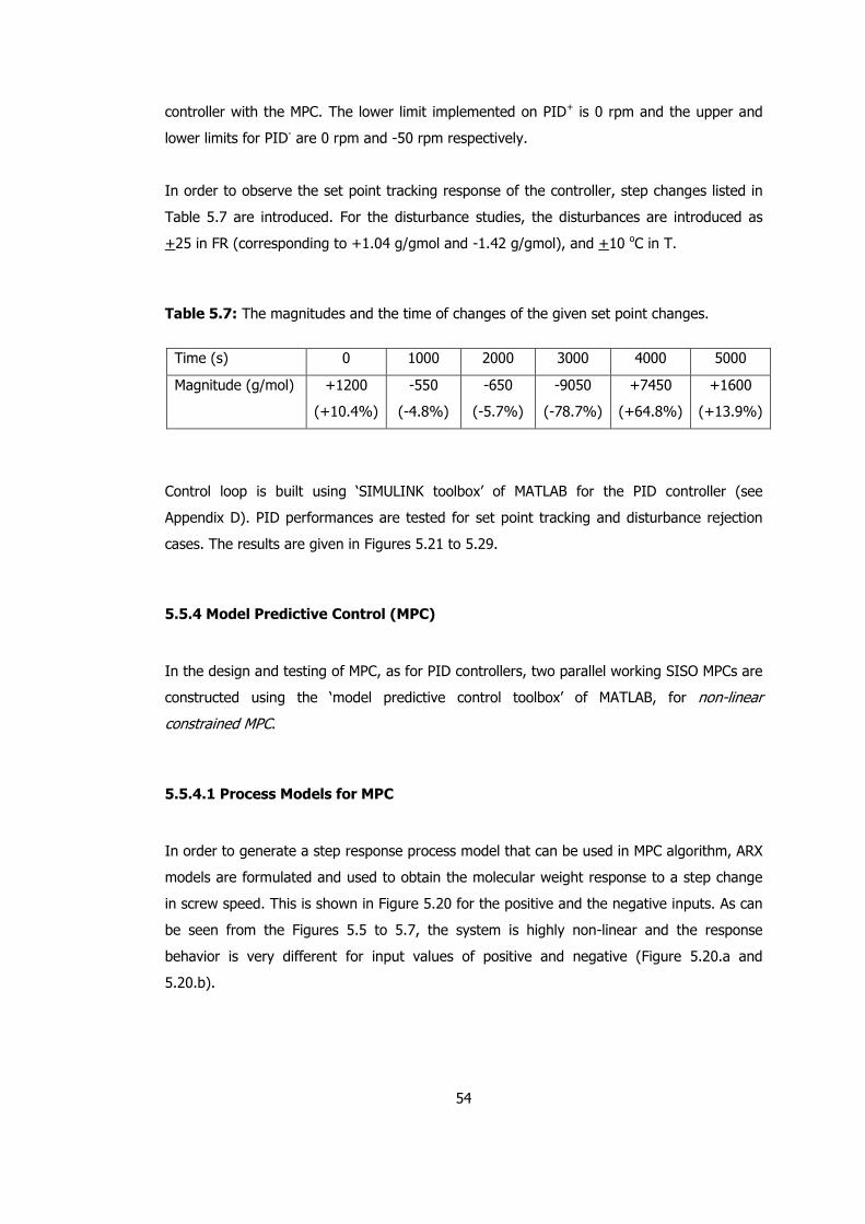
54
controller with the MPC. The lower limit implemented on PID+ is 0 rpm and the upper and
lower limits for PID- are 0 rpm and -50 rpm respectively.
In order to observe the set point tracking response of the controller, step changes listed in
Table 5.7 are introduced. For the disturbance studies, the disturbances are introduced as
+25 in FR (corresponding to +1.04 g/gmol and -1.42 g/gmol), and +10 oC in T.
Table 5.7: The magnitudes and the time of changes of the given set point changes.
Time (s) 0 1000 2000 3000 4000 5000
Magnitude (g/mol) +1200
(+10.4%)
-550
(-4.8%)
-650
(-5.7%)
-9050
(-78.7%)
+7450
(+64.8%)
+1600
(+13.9%)
Control loop is built using ‘SIMULINK toolbox’ of MATLAB for the PID controller (see
Appendix D). PID performances are tested for set point tracking and disturbance rejection
cases. The results are given in Figures 5.21 to 5.29.
5.5.4 Model Predictive Control (MPC)
In the design and testing of MPC, as for PID controllers, two parallel working SISO MPCs are
constructed using the ‘model predictive control toolbox’ of MATLAB, for non-linear
constrained MPC.
5.5.4.1 Process Models for MPC
In order to generate a step response process model that can be used in MPC algorithm, ARX
models are formulated and used to obtain the molecular weight response to a step change
in screw speed. This is shown in Figure 5.20 for the positive and the negative inputs. As can
be seen from the Figures 5.5 to 5.7, the system is highly non-linear and the response
behavior is very different for input values of positive and negative (Figure 5.20.a and
5.20.b).
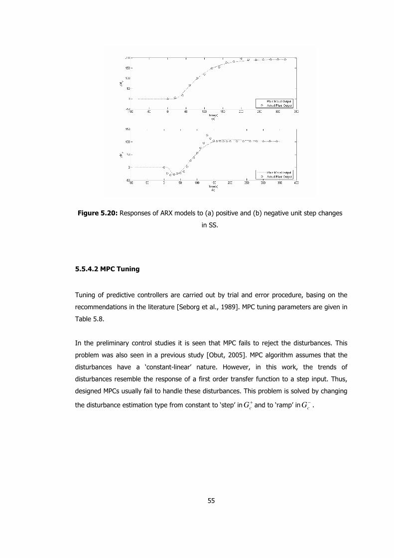
55
Figure 5.20: Responses of ARX models to (a) positive and (b) negative unit step changes
in SS.
5.5.4.2 MPC Tuning
Tuning of predictive controllers are carried out by trial and error procedure, basing on the
recommendations in the literature [Seborg et al., 1989]. MPC tuning parameters are given in
Table 5.8.
In the preliminary control studies it is seen that MPC fails to reject the disturbances. This
problem was also seen in a previous study [Obut, 2005]. MPC algorithm assumes that the
disturbances have a ‘constant-linear’ nature. However, in this work, the trends of
disturbances resemble the response of a first order transfer function to a step input. Thus,
designed MPCs usually fail to handle these disturbances. This problem is solved by changing
the disturbance estimation type from constant to ‘step’ in +cG and to ‘ramp’ in −
cG .
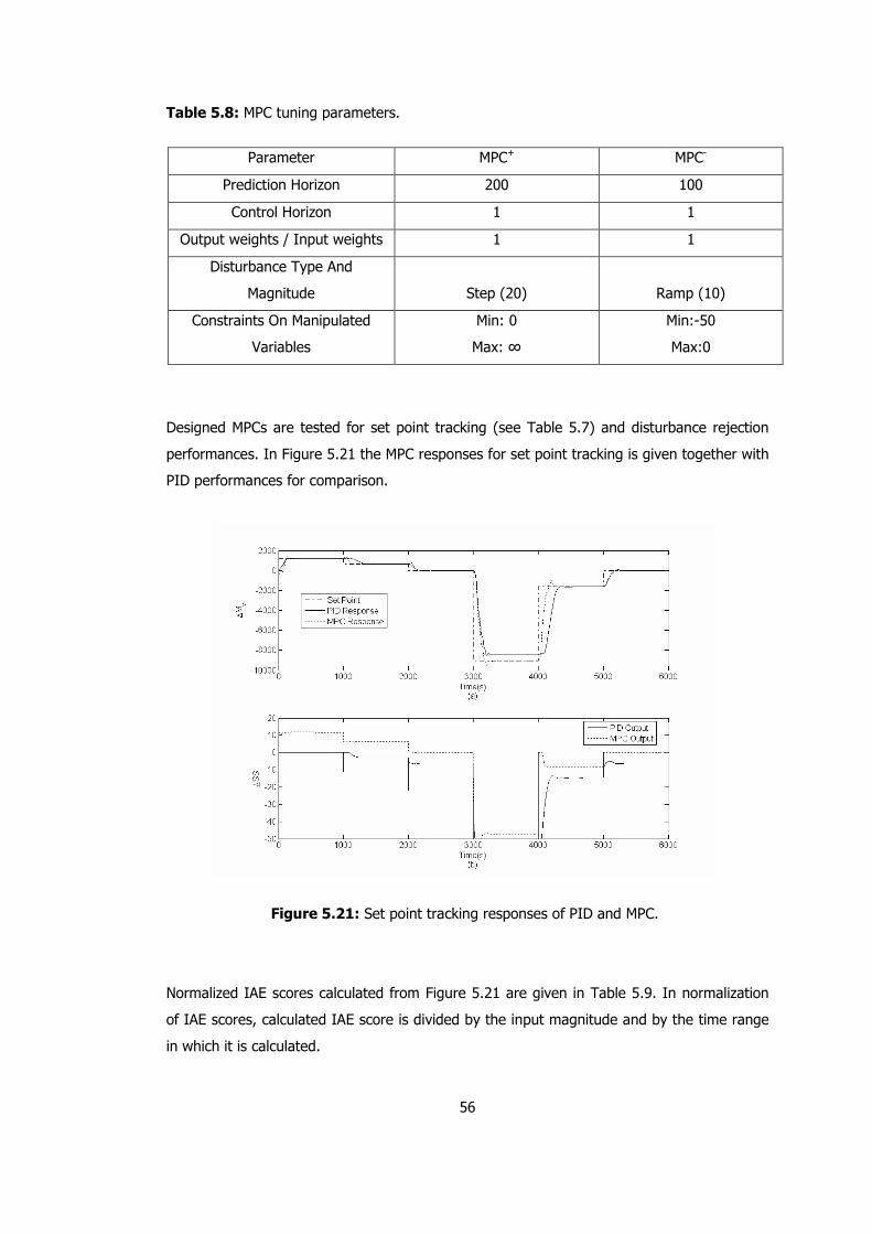
56
Table 5.8: MPC tuning parameters.
Parameter MPC+ MPC-
Prediction Horizon 200 100
Control Horizon 1 1
Output weights / Input weights 1 1
Disturbance Type And
Magnitude Step (20) Ramp (10)
Constraints On Manipulated
Variables
Min: 0
Max: ∞
Min:-50
Max:0
Designed MPCs are tested for set point tracking (see Table 5.7) and disturbance rejection
performances. In Figure 5.21 the MPC responses for set point tracking is given together with
PID performances for comparison.
Figure 5.21: Set point tracking responses of PID and MPC.
Normalized IAE scores calculated from Figure 5.21 are given in Table 5.9. In normalization
of IAE scores, calculated IAE score is divided by the input magnitude and by the time range
in which it is calculated.
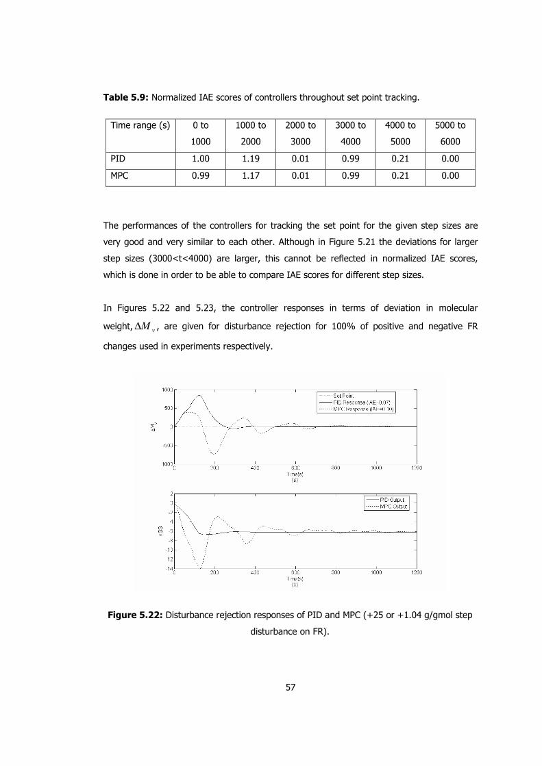
57
Table 5.9: Normalized IAE scores of controllers throughout set point tracking.
Time range (s) 0 to
1000
1000 to
2000
2000 to
3000
3000 to
4000
4000 to
5000
5000 to
6000
PID 1.00 1.19 0.01 0.99 0.21 0.00
MPC 0.99 1.17 0.01 0.99 0.21 0.00
The performances of the controllers for tracking the set point for the given step sizes are
very good and very similar to each other. Although in Figure 5.21 the deviations for larger
step sizes (3000<t<4000) are larger, this cannot be reflected in normalized IAE scores,
which is done in order to be able to compare IAE scores for different step sizes.
In Figures 5.22 and 5.23, the controller responses in terms of deviation in molecular
weight, vM∆ , are given for disturbance rejection for 100% of positive and negative FR
changes used in experiments respectively.
Figure 5.22: Disturbance rejection responses of PID and MPC (+25 or +1.04 g/gmol step
disturbance on FR).
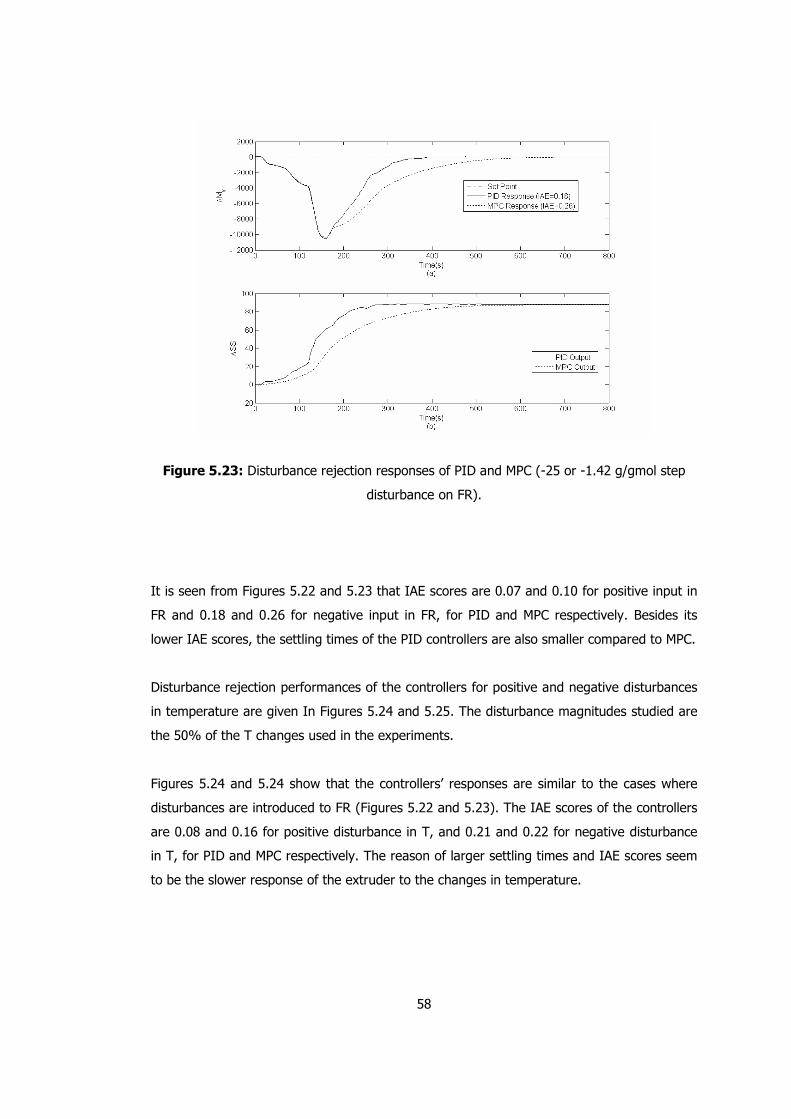
58
Figure 5.23: Disturbance rejection responses of PID and MPC (-25 or -1.42 g/gmol step
disturbance on FR).
It is seen from Figures 5.22 and 5.23 that IAE scores are 0.07 and 0.10 for positive input in
FR and 0.18 and 0.26 for negative input in FR, for PID and MPC respectively. Besides its
lower IAE scores, the settling times of the PID controllers are also smaller compared to MPC.
Disturbance rejection performances of the controllers for positive and negative disturbances
in temperature are given In Figures 5.24 and 5.25. The disturbance magnitudes studied are
the 50% of the T changes used in the experiments.
Figures 5.24 and 5.24 show that the controllers’ responses are similar to the cases where
disturbances are introduced to FR (Figures 5.22 and 5.23). The IAE scores of the controllers
are 0.08 and 0.16 for positive disturbance in T, and 0.21 and 0.22 for negative disturbance
in T, for PID and MPC respectively. The reason of larger settling times and IAE scores seem
to be the slower response of the extruder to the changes in temperature.
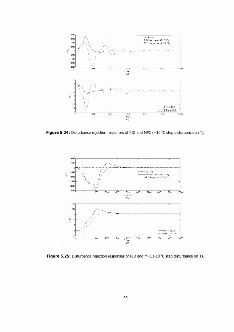
59
Figure 5.24: Disturbance rejection responses of PID and MPC (+10 oC step disturbance on T).
Figure 5.25: Disturbance rejection responses of PID and MPC (-10 oC step disturbance on T).
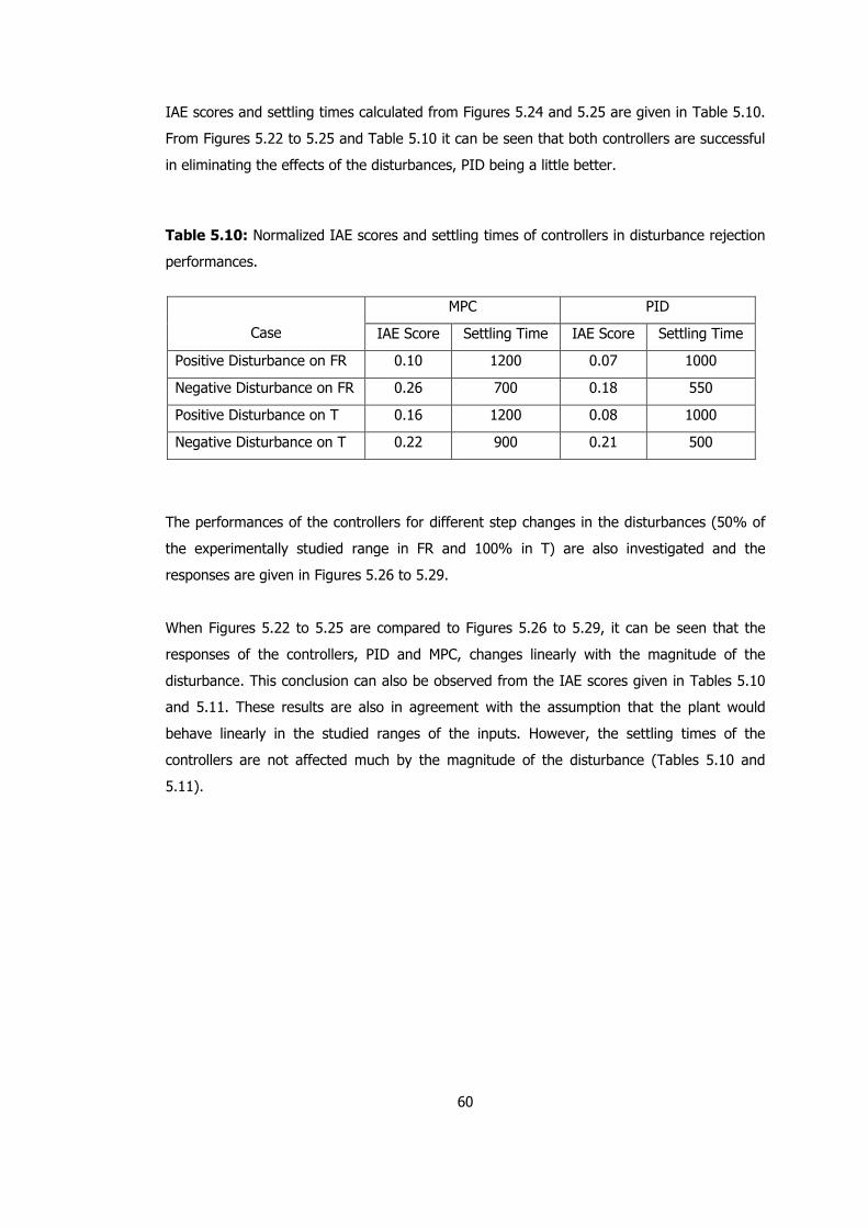
60
IAE scores and settling times calculated from Figures 5.24 and 5.25 are given in Table 5.10.
From Figures 5.22 to 5.25 and Table 5.10 it can be seen that both controllers are successful
in eliminating the effects of the disturbances, PID being a little better.
Table 5.10: Normalized IAE scores and settling times of controllers in disturbance rejection
performances.
MPC PID
Case IAE Score Settling Time IAE Score Settling Time
Positive Disturbance on FR 0.10 1200 0.07 1000
Negative Disturbance on FR 0.26 700 0.18 550
Positive Disturbance on T 0.16 1200 0.08 1000
Negative Disturbance on T 0.22 900 0.21 500
The performances of the controllers for different step changes in the disturbances (50% of
the experimentally studied range in FR and 100% in T) are also investigated and the
responses are given in Figures 5.26 to 5.29.
When Figures 5.22 to 5.25 are compared to Figures 5.26 to 5.29, it can be seen that the
responses of the controllers, PID and MPC, changes linearly with the magnitude of the
disturbance. This conclusion can also be observed from the IAE scores given in Tables 5.10
and 5.11. These results are also in agreement with the assumption that the plant would
behave linearly in the studied ranges of the inputs. However, the settling times of the
controllers are not affected much by the magnitude of the disturbance (Tables 5.10 and
5.11).
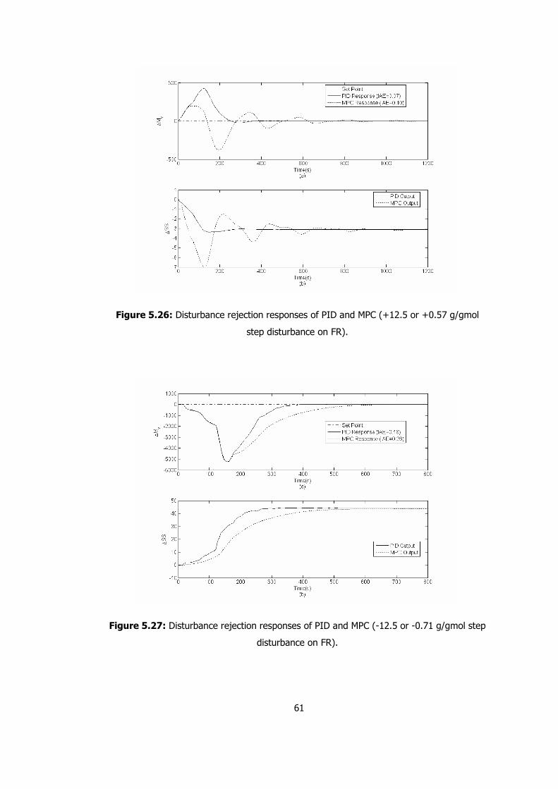
61
Figure 5.26: Disturbance rejection responses of PID and MPC (+12.5 or +0.57 g/gmol
step disturbance on FR).
Figure 5.27: Disturbance rejection responses of PID and MPC (-12.5 or -0.71 g/gmol step
disturbance on FR).
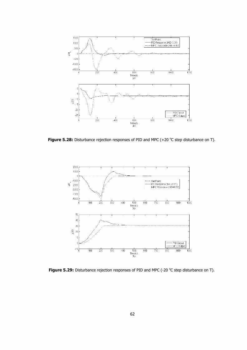
62
Figure 5.28: Disturbance rejection responses of PID and MPC (+20 oC step disturbance on T).
Figure 5.29: Disturbance rejection responses of PID and MPC (-20 oC step disturbance on T).
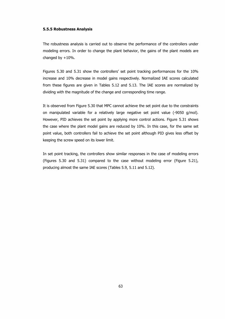
63
5.5.5 Robustness Analysis
The robustness analysis is carried out to observe the performance of the controllers under
modeling errors. In order to change the plant behavior, the gains of the plant models are
changed by +10%.
Figures 5.30 and 5.31 show the controllers’ set point tracking performances for the 10%
increase and 10% decrease in model gains respectively. Normalized IAE scores calculated
from these figures are given in Tables 5.12 and 5.13. The IAE scores are normalized by
dividing with the magnitude of the change and corresponding time range.
It is observed from Figure 5.30 that MPC cannot achieve the set point due to the constraints
on manipulated variable for a relatively large negative set point value (-9050 g/mol).
However, PID achieves the set point by applying more control actions. Figure 5.31 shows
the case where the plant model gains are reduced by 10%. In this case, for the same set
point value, both controllers fail to achieve the set point although PID gives less offset by
keeping the screw speed on its lower limit.
In set point tracking, the controllers show similar responses in the case of modeling errors
(Figures 5.30 and 5.31) compared to the case without modeling error (Figure 5.21),
producing almost the same IAE scores (Tables 5.9, 5.11 and 5.12).
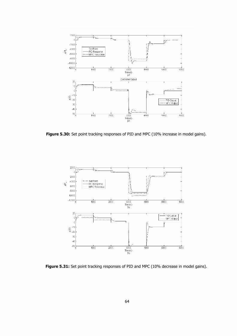
64
Figure 5.30: Set point tracking responses of PID and MPC (10% increase in model gains).
Figure 5.31: Set point tracking responses of PID and MPC (10% decrease in model gains).
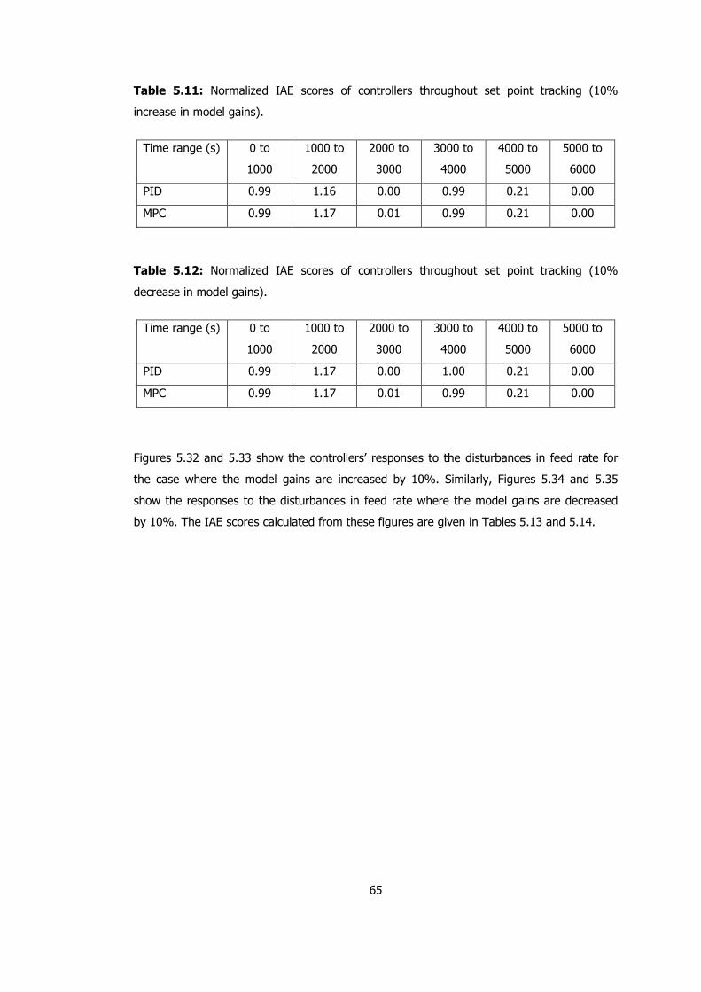
65
Table 5.11: Normalized IAE scores of controllers throughout set point tracking (10%
increase in model gains).
Time range (s) 0 to
1000
1000 to
2000
2000 to
3000
3000 to
4000
4000 to
5000
5000 to
6000
PID 0.99 1.16 0.00 0.99 0.21 0.00
MPC 0.99 1.17 0.01 0.99 0.21 0.00
Table 5.12: Normalized IAE scores of controllers throughout set point tracking (10%
decrease in model gains).
Time range (s) 0 to
1000
1000 to
2000
2000 to
3000
3000 to
4000
4000 to
5000
5000 to
6000
PID 0.99 1.17 0.00 1.00 0.21 0.00
MPC 0.99 1.17 0.01 0.99 0.21 0.00
Figures 5.32 and 5.33 show the controllers’ responses to the disturbances in feed rate for
the case where the model gains are increased by 10%. Similarly, Figures 5.34 and 5.35
show the responses to the disturbances in feed rate where the model gains are decreased
by 10%. The IAE scores calculated from these figures are given in Tables 5.13 and 5.14.
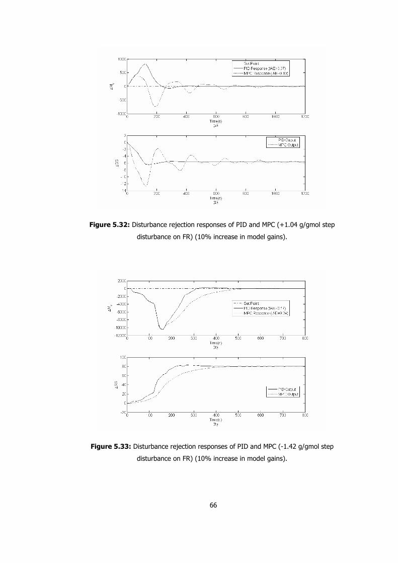
66
Figure 5.32: Disturbance rejection responses of PID and MPC (+1.04 g/gmol step
disturbance on FR) (10% increase in model gains).
Figure 5.33: Disturbance rejection responses of PID and MPC (-1.42 g/gmol step
disturbance on FR) (10% increase in model gains).
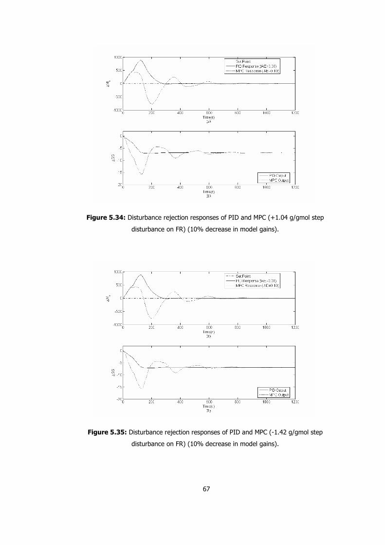
67
Figure 5.34: Disturbance rejection responses of PID and MPC (+1.04 g/gmol step
disturbance on FR) (10% decrease in model gains).
Figure 5.35: Disturbance rejection responses of PID and MPC (-1.42 g/gmol step
disturbance on FR) (10% decrease in model gains).
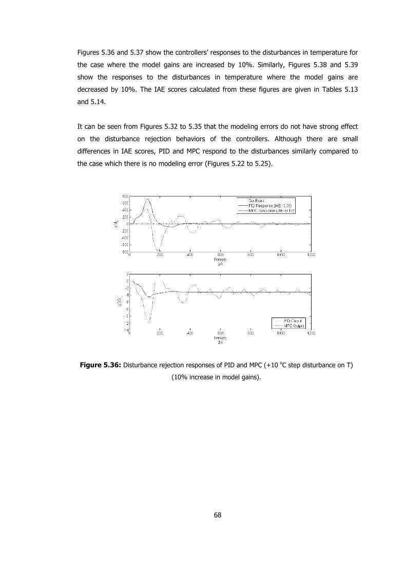
68
Figures 5.36 and 5.37 show the controllers’ responses to the disturbances in temperature for
the case where the model gains are increased by 10%. Similarly, Figures 5.38 and 5.39
show the responses to the disturbances in temperature where the model gains are
decreased by 10%. The IAE scores calculated from these figures are given in Tables 5.13
and 5.14.
It can be seen from Figures 5.32 to 5.35 that the modeling errors do not have strong effect
on the disturbance rejection behaviors of the controllers. Although there are small
differences in IAE scores, PID and MPC respond to the disturbances similarly compared to
the case which there is no modeling error (Figures 5.22 to 5.25).
Figure 5.36: Disturbance rejection responses of PID and MPC (+10 oC step disturbance on T)
(10% increase in model gains).
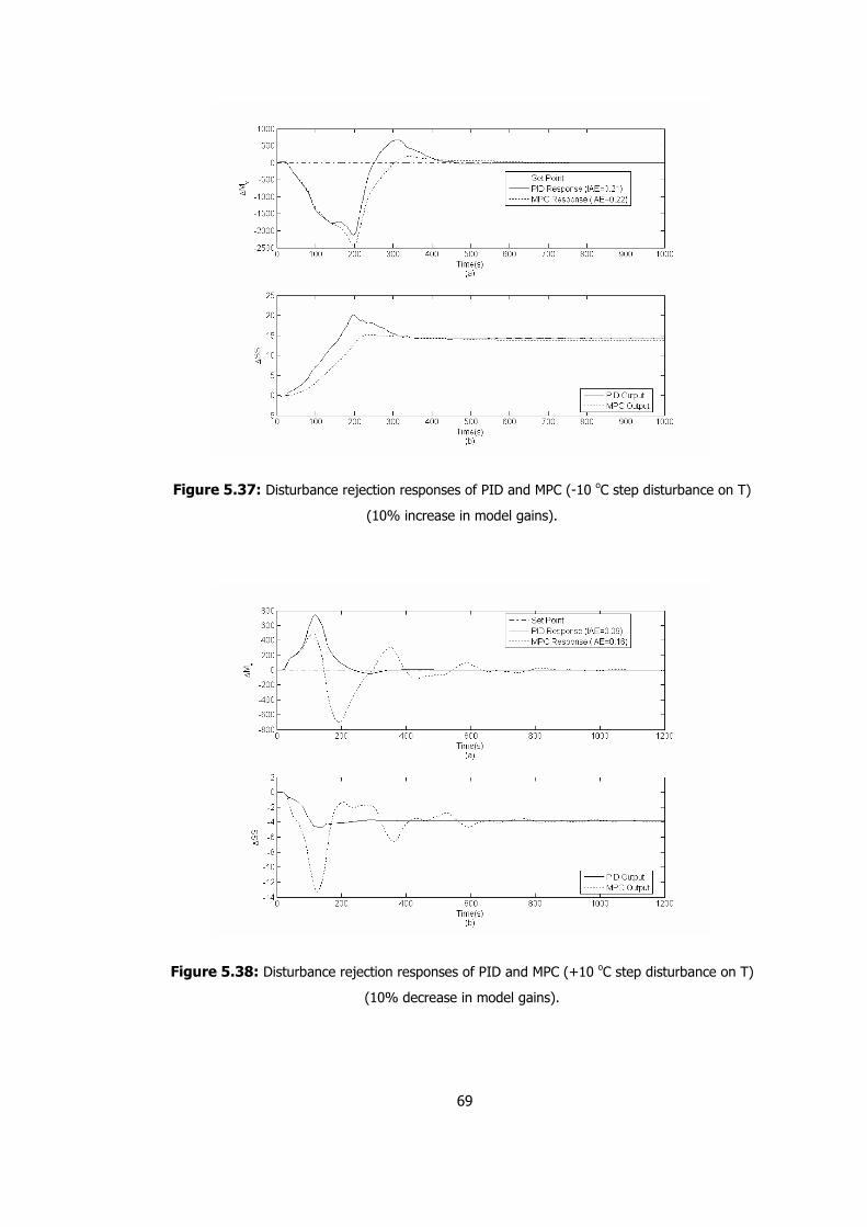
69
Figure 5.37: Disturbance rejection responses of PID and MPC (-10 oC step disturbance on T)
(10% increase in model gains).
Figure 5.38: Disturbance rejection responses of PID and MPC (+10 oC step disturbance on T)
(10% decrease in model gains).
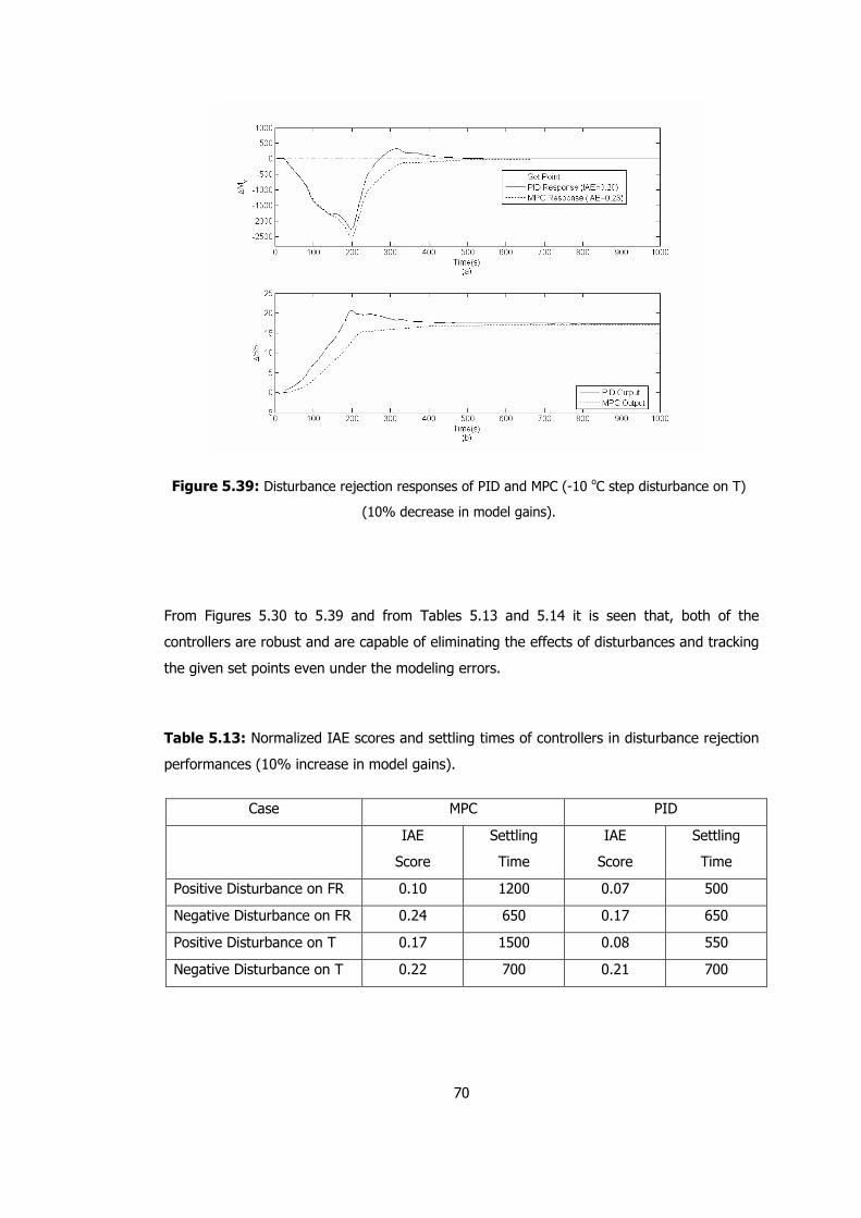
70
Figure 5.39: Disturbance rejection responses of PID and MPC (-10 oC step disturbance on T)
(10% decrease in model gains).
From Figures 5.30 to 5.39 and from Tables 5.13 and 5.14 it is seen that, both of the
controllers are robust and are capable of eliminating the effects of disturbances and tracking
the given set points even under the modeling errors.
Table 5.13: Normalized IAE scores and settling times of controllers in disturbance rejection
performances (10% increase in model gains).
Case MPC PID
IAE
Score
Settling
Time
IAE
Score
Settling
Time
Positive Disturbance on FR 0.10 1200 0.07 500
Negative Disturbance on FR 0.24 650 0.17 650
Positive Disturbance on T 0.17 1500 0.08 550
Negative Disturbance on T 0.22 700 0.21 700

71
Table 5.14: Normalized IAE scores and settling times of controllers in disturbance rejection
performances (10% decrease in models gains).
Case MPC PID
IAE
Score
Settling
Time
IAE
Score
Settling
Time
Positive Disturbance on FR 0.10 1200 0.08 600
Negative Disturbance on FR 0.29 800 0.20 650
Positive Disturbance on T 0.16 1200 0.09 600
Negative Disturbance on T 0.23 650 0.20 650

72
CHAPTER VI
CONCLUSIONS
In this study, experimental and theoretical studies are done to design an inferential control
scheme for the feedback control of RPET degradation during extrusion process. The basic
conclusions arrived are as follows:
• Degradation of PET is found to be highly nonlinear and it is affected by different
variables such as barrel temperatures and residence time spent in the extruder.
• The product quality is considered to be determined by molecular weight, Mv, and can be
measured indirectly by intrinsic viscosity ([η]).
• Dynamic experiments revealed that the extrusion process is highly nonlinear. It shows
different behaviors for the positive or negative deviations of the inputs.
• Convolution models are selected to be the best and to be used in simulations rather
than single or dual transfer functions of different properties.
• In the control system screw speed is evaluated to be manipulated variable using the
SVD analysis while barrel temperature and feed flow rate left to be probable
disturbances.
• In the control system designed, two different controllers ( +cG and −
cG ) are used for
positive and negative parts of the process model.
• PID and MPC controllers’ performances are found to be successful for set point tracking
and disturbance rejection cases.
• PID and MPC controllers are proven to be robust under modeling errors (+10%).
• The designed inferential control scheme can be utilized in controlling the product quality
in terms of molecular weight both with PID and MPC, once the off-line necessary data
for the estimator is obtained.
73
REFERENCES
Assadi, R., Colin, X., Verdu, J., (2004), “Irreversible structural changes during PET recycling
by extrusion”, Polymer 45, 4403-4412
Awaja, F., Daver, F., (2004), “Recycled poly(ethylene terephthalate) chain extension by a
reactive extrusion process”, Poly. Eng. Sci. 44, 1579-1587
Awaja, F., Dumitru, P., (2005), “Recycling of PET”, Eur. Ploym. J. 41, 1453-1477
Bahar, A., Özgen, C, Leblebicioğlu, K., Halıcı, U., (2004), “ Artificial neural network design
for the inferential model predictive control of an industrial distillation column”, Ind.
Eng. Chem. Res. 43, 6102-6111
Berkowitz, S., (1984), “Viscosity-molecular weight relationships for poly(ethylene
terephthalate) in hexafluoroisopropanol-pentafluorophenol using SEC-LALLS”, J.
App. Poly. Sci 29, 4353-4361
Biagiola, S.I., Solsona, J.A., Figueroa, J.L., (2005), “Use of state estimation for inferential
nonlinear MPC: a case study”, Chem. Eng. J. 106, 13-24
Brandrub, J., Immergut, E.H., (1989), “Polymer Handbook”, 3rd Ed., Wiley Inc.
Brengel, D., Seider, W.D., (1989), “Multistep nonlinear predictive controller”, Ind. Eng.
Chem. Res. 28, 1812-1822
Broadhead, T.O., Patterson, W.I., Dealy, J.M., (1996), “Closed loop viscosity control of
reactive extrusion with an in-line rheometer”, Polym. Eng. Sci. 36, 2840-2851
Camacho, E.F. and Bordons, C. (2000), “Model Predictive Control”, Springer Verlag London
Lim.
Chelsea Center For Recycling And Economic Development (University of Massachusetts),
(2000), “ Potential end uses for polyester fiber waste: A laboratory study”,
Technical Report #33.
Chen, Z.L., Chao, P.Y., Chiu S.H., (2003), “Proposal of an empirical viscosity model for
quality control in the polymer extrusion process”, Polymer Testing 22, 601-607
Choulak, S., Couenne, F., Le Gorrec, Y., Jallut, C., Cassagnau, P., Michel, A., (2004),
“Generic dynamic model for simulation and control of reactive extrusion”, Ind. Eng.
Chem. Res. 43, 7373-7382
Costin, M.H., Taylor, P.A., Wright, J.D., (1982), “A critical review of dynamic modeling and
control of plasticating extruders” Polym. Eng. Sci. 22, 393-401
74
Costin, M.H., Taylor, P.A., Wright, J.D., (1982), “On the dynamics and control of a
plasticating extruder”, Polym. Eng. Sci. 22, 1095-1106
De Ruyck, H., (1997), “Modeling of the residence time distribution in a twin screw extruder”,
J. Food Eng. 32, 375-390
Doyle III, F.J., (1998), “Nonlinear inferential control for process applications”, J. Proc. Con.
8 (5-6), 339-353
Elsey, J., Reipenhausen, J., McKay, B., Barton, G.W., Willis, M., (1997), “Modeling and
control of food extrusion process”, Computers Chem. Eng. 21, s361-s366
Fisher, E.G., (1976), “Extrusion of plastics”, Hazell Watson And Viney Ltd.
Garcia, C.E., Prett, D.M., Morari, M., (1989), “Model predictive control: Theory and practice
– a survey”, Automatica 25, 335-348
Haley, T.A., Mulvaney S.J., (2000), “On-line system identification and control design of an
extrusion cooking process: Part II. Model predictive and inferential control design”,
Food Control 11, 121-129
Hassan, G.A., Parnaby, J., (1981), “Model reference optimal steady-state adaptive computer
control of plastics extrusion process”, Polym. Eng. Sci. 21, 276-284
Incarnato, L., Scarfato, P., Di Maio, L., Acierno, D., (2000), “Structure and rheology of
recycled PET modified by reactive extrusion”, Polymer 41, 6825-6831
Karayannidis P G. and Psalida E A., (2000), “Chain extension of recycled poly(ethylene
terephthalate) with 2,2 -(1,4-phenylene)bis(2-oxazoline)”, J. Appl. Polym. Sci. 77,
2206-2211
Kent, R.J., (1998), “Report 104: Plastics profile extrusion”, Rapra Review Reports, Vol. 9
No.8
Klema, V.C., Laub, A.J., (1980), “The singular value decomposition: Its computation and
some applications”, IEEE Trans. Automatic Cont. 25, 164-176
Lee, S.J., Hong, C., Han, T., Kang, J., Kwon, Y.A., (2002), “Application of fuzzy control to
start-up of twin screw extruder”, Food Control 13, 301-306
Luyben W.L., (1990), “Process modeling and control for chemical engineers”, 2nd Ed.,
McGraw-Hill Book Co.
Luyben, W.L., (2006), “Evaluation of criteria for selecting temperature control trays in
distillation columns”, J. Proc. Cont. 16, 115-134
Marchetti, J.L., Mellichamp, D.A., Seborg, D.E., (1983), “Predictive control based on discrete
convolution models”, In. Eng. Chem. 22, 488-495
Maurath, P.R., Mellichamp D.A., Seborg, D.E., (1988), “Predictive controller design for
single-input/single-output (SISO) systems”, Ind. Eng. Chem. Res. 27, 956-963
75
Meziou, A.M., Deshpande, P.B., Cozewith, C., Silverman, N.I., Morrison, W.G., (1996),
“Dynamic matrix control of an ethylene-propylene-diene polymerization reactor”,
Ind. Eng. Chem. Res. 35, 164-168
Morningred, J.D., Paden, B.E., Seborg, D.E., Mellichamp, D.A., (1992), “An adaptive
nonlinear predictive control”, Chem. Eng. Sci. 47, 755-762
Mudalamane, R., Bigio, D.I., (2003), “Process variations and the transient behavior of
extruders”, AIChE J. 49(12), 3150-3160
Nied, S.A., Budman, H.M., Tzoganakis, C., (2000), “Control of a LDPE reactive extrusion
process”, Cont. Eng. Prac. 8, 911-920
Obut, S., (2005), “Control of pH neutralization reactor of a waste water treatment system
using identification reactor”, M.Sc. Thesis, Chem. Eng Dept. METU
Ogawa, M., Ohshima, M., Morinaga, K., Watanabe, F., (1999), “Quality inferential control of
an industrial high density polyethylene process”, J. Proc. Con. 9, 51-59
Oromiehie, A., Mamizadeh, A., (2004), “Recycling PET beverage bottles and improving
properties”, Polym. Int. 53, 728-732
Özkan. L., Kothare, M.V., Georgakis, C., (2003), “Control of solution polymerization reactor
using multi-model predictive control”, Chem. Eng. Sci. 58, 1207-1221
Pabedinskas, A., Cluett, W.R., Balke, S.T., (1989), “Process control for polyprobylene
degradation during reactive extrusion”, Polym. Eng. Sci. 29, 993-1003
Parnaby, J., Kochhar, A. K., Wood, B., (1975), “Development of computer strategies for
plastic extruders”, Polym. Eng. Sci. 15, 594-605
Pawlak, A., Pluta, M., Morawiec, J., Galeski, A., Pracella, M., (2000), “Characterization of
scrap poly(ethylene terephthalate)”, Eur. Poly. J. 36, 1875-1884
PETCORE, http://www.petcore.org, last accessed on 7.8.2006
Previdi, F., Savaresi, S.M., Panarotto, A., (2006), “Design of a feedback control system for
real-time control of flow in a single-screw extruder”, Con. Eng. Prac., 14, 1111-1121
Rauwendaal, C., (1998), “Understanding extrusion”, Carl Hanser Verlag
Rojas, O.J., Goodwin, G.C., Seron, M.M., Feuer, A., (2004), “An SCD based strategy for
receding horizon control of input constrained linear systems”, Int. J. Robust
Nonlinear Cont. 14, 1207-1226
Rosen, S.L., (1982), “Fundamental principles of polymeric materials”, Wiley Inc.
Seborg, D.E., Edgar, T.F., Mellichamp, D.A., (1989), “Process dynamics and control”, Wiley
Inc.
Smith, J.M., Janssen, L.P.B.M., Koning, W.L., Abeln, P.P.J., (1978), “The operating
characteristics of twin screw extruders”, Polym. Eng. Sci. 18, 660-667
76
Spinace, M.A., De Paoli, M.A., (2000), “Characterization of poly(ethylene terephtalate) after
multiple processing cycles”, App. Poly. Sci. 80, 20-25
Stephanopoulos, G., (1984), “Chemical process control – an introduction to theory and
practice”, Prentice-Hall Inc.
Tanrattanakul, V., Hiltner, A., Baer, E., Perkins, W.G., Massey, F.L., Moet, A., (1996),
“Toughening PET by blending with a functionalized SEBS block copolymer”, Polymer
38, 2191-2200
Tanttu, J.T., Zchuchenko, A.I., Koivo, H.N., (1989), “A simulation study of the self-tuning
control of a plastics extruder”, Control and Applications, ICCON, IEEE Int. Conf.
Torres, N., Robin, J.J., Boutevin B., (2000), “Chemical modification of virgin and recycled
poly(ethylene terephthalate) by adding chain extenders during processing”, App.
Poly. Sci. 79, 1816-1824
Wang, L. Gawthrop, P, Chessari, C., Podsiadly, T, Giles,A., (2004), “Indirect approach to
continuous system identification of food extruder”, J. Pro. Cont. 14, 603-615
Wang, L., Chessari, C., Karpiel, E., (2001),” Inferential control of product quality attributes –
application to food cooking extrusion process”, J. Proc. Con. 11, 621-636
Wang, Y., Tan, J., (2000), “Dual-target predictive control and application in food extrusion”,
Cont. Eng. Prac. 8, 1055-1062
Wikipedia, http://en.wikipedia.org/wiki/Plastic_recycling, last accessed on 7.8.2006
Wikipedia, http://en.wikipedia.org/wiki/Polyethylene_terephthalate, last accessed on
7.8.2006
Wikipedia, http://en.wikipedia.org/wiki/Recycling_of_PET_Bottles, last accessed on 7.8.2006
Wikipedia, http://en.wikipedia.org/wiki/Singular_value_decomposition, last accessed on
8.2.2006
Xanthos, M., (1992), “Reactive extrusion – principles and practice”, Carl Hanser Verlag
Xiao, K., Tzoganakis, C., Budman, H., (2001), “Control of coating properties of LDPE
through melt strength measurements”, Cont. Eng. Prac. 9, 357-366
Yang, B., Lee, L.J., (1986), “Process control of polymer extrusion. Part I: Feedback control”,
Polym. Eng. Sci. 26, 197-204
Zheng, D., Hoo, K.A., (2004), “System identification and model-based control for distributed
parameter systems”, Comp. Chem. Eng. 28, 1361-1375
77
APPENDIX A
MOLECULAR WEIGHT DETERMINATION
Viscosities1 of polymer solutions are usually measured in glass viscometers (Figure D.1), in
which the solution flows through a capillary tube by gravity. Two common types are Ostwald
and Ubbelohde viscometers. The Ubbelohde viscometer has the advantage that the flowing
solution is not affected by the amount of the liquid in the reservoir. Thus, the concentration
of the solution can be changed directly in the viscometer.
A.1 Molecular Weight Determination
The molecular weights (Mv) of the collected samples are determined by dilute solution
viscometry, using a Ubbelohde type viscometer.
0.06 gram of sample is weighted and dissolved in 6 ml of trifluoroacetic acid (TFA) in a test
tube, giving 1 g/dl concentration.
Initially, the flow time of pure solvent (t0) between two mark points is measured using a
chronometer, and recorded. The initial amount of pure solvent (TFA) in the viscometer is 7
ml. Measurement of t0 is repeated until same ‘minute:second’ value is read with the previous
flow (or flow time became constant).
1 “Since polymer solutions are non-Newtonian, intrinsic viscosity must be defined, strictly speaking, in terms of the
zero-shear or lower Newtonian viscosity. This is rarely a problem because the low shear rates in the usual
glassware viscometers give just that. Occasionally, however, extrapolation to zero-shear condition is required”
[Rosen, 1982].
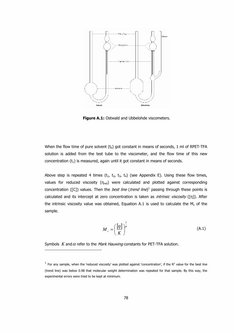
78
Figure A.1: Ostwald and Ubbelohde viscometers.
When the flow time of pure solvent (t0) got constant in means of seconds, 1 ml of RPET-TFA
solution is added from the test tube to the viscometer, and the flow time of this new
concentration (t1) is measured, again until it got constant in means of seconds.
Above step is repeated 4 times (t1, t2, t3, t4) (see Appendix E). Using these flow times,
values for reduced viscosity (ηred) were calculated and plotted against corresponding
concentration ([C]) values. Then the best line (trend line)1 passing through these points is
calculated and its intercept at zero concentration is taken as intrinsic viscosity ([η]). After
the intrinsic viscosity value was obtained, Equation A.1 is used to calculate the Mv of the
sample.
[ ] αη1
=
KM v (A.1)
Symbols K andα refer to the Mark Hauwing constants for PET-TFA solution.
1 For any sample, when the ‘reduced viscosity’ was plotted against ‘concentration’, if the R2 value for the best line
(trend line) was below 0.98 that molecular weight determination was repeated for that sample. By this way, the
experimental errors were tried to be kept at minimum.
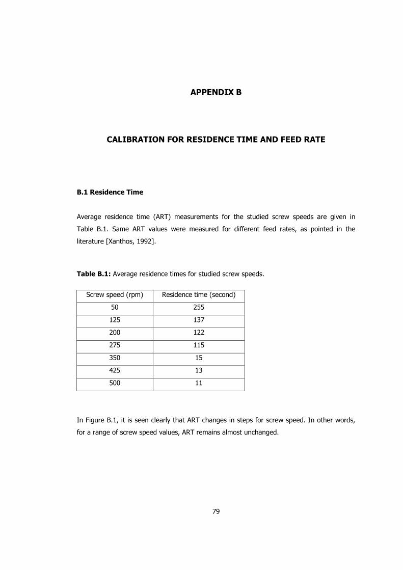
79
APPENDIX B
CALIBRATION FOR RESIDENCE TIME AND FEED RATE
B.1 Residence Time
Average residence time (ART) measurements for the studied screw speeds are given in
Table B.1. Same ART values were measured for different feed rates, as pointed in the
literature [Xanthos, 1992].
Table B.1: Average residence times for studied screw speeds.
Screw speed (rpm) Residence time (second)
50 255
125 137
200 122
275 115
350 15
425 13
500 11
In Figure B.1, it is seen clearly that ART changes in steps for screw speed. In other words,
for a range of screw speed values, ART remains almost unchanged.
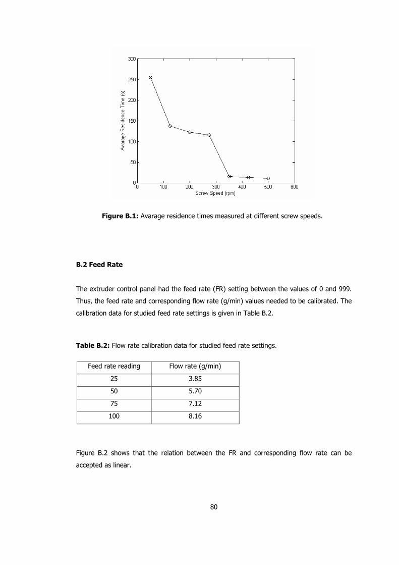
80
Figure B.1: Avarage residence times measured at different screw speeds.
B.2 Feed Rate
The extruder control panel had the feed rate (FR) setting between the values of 0 and 999.
Thus, the feed rate and corresponding flow rate (g/min) values needed to be calibrated. The
calibration data for studied feed rate settings is given in Table B.2.
Table B.2: Flow rate calibration data for studied feed rate settings.
Feed rate reading Flow rate (g/min)
25 3.85
50 5.70
75 7.12
100 8.16
Figure B.2 shows that the relation between the FR and corresponding flow rate can be
accepted as linear.
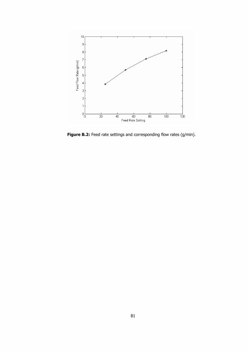
81
Figure B.2: Feed rate settings and corresponding flow rates (g/min).
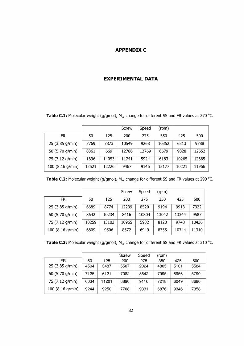
82
APPENDIX C
EXPERIMENTAL DATA
Table C.1: Molecular weight (g/gmol), Mv, change for different SS and FR values at 270 oC.
Screw Speed (rpm)
FR 50 125 200 275 350 425 500
25 (3.85 g/min) 7769 7873 10549 9268 10352 6313 9788
50 (5.70 g/min) 8361 669 12786 12769 6679 9828 12652
75 (7.12 g/min) 1696 14053 11741 5924 6183 10265 12665
100 (8.16 g/min) 12521 12226 9467 9146 13177 10221 11966
Table C.2: Molecular weight (g/gmol), Mv, change for different SS and FR values at 290 oC.
Screw Speed (rpm)
FR 50 125 200 275 350 425 500
25 (3.85 g/min) 6689 8774 12239 8520 9194 9913 7322
50 (5.70 g/min) 8642 10234 8416 10804 13042 13344 9587
75 (7.12 g/min) 10259 13103 10965 5932 8120 9748 10436
100 (8.16 g/min) 6809 9506 8572 6949 8355 10744 11310
Table C.3: Molecular weight (g/gmol), Mv, change for different SS and FR values at 310 oC.
Screw Speed (rpm)
FR 50 125 200 275 350 425 500
25 (3.85 g/min) 4504 3487 5507 2024 4805 5101 5584
50 (5.70 g/min) 7125 6121 7082 8642 7995 8956 5790
75 (7.12 g/min) 6034 11201 6890 9116 7218 6049 8680
100 (8.16 g/min) 9244 9250 7708 9331 6876 9346 7358
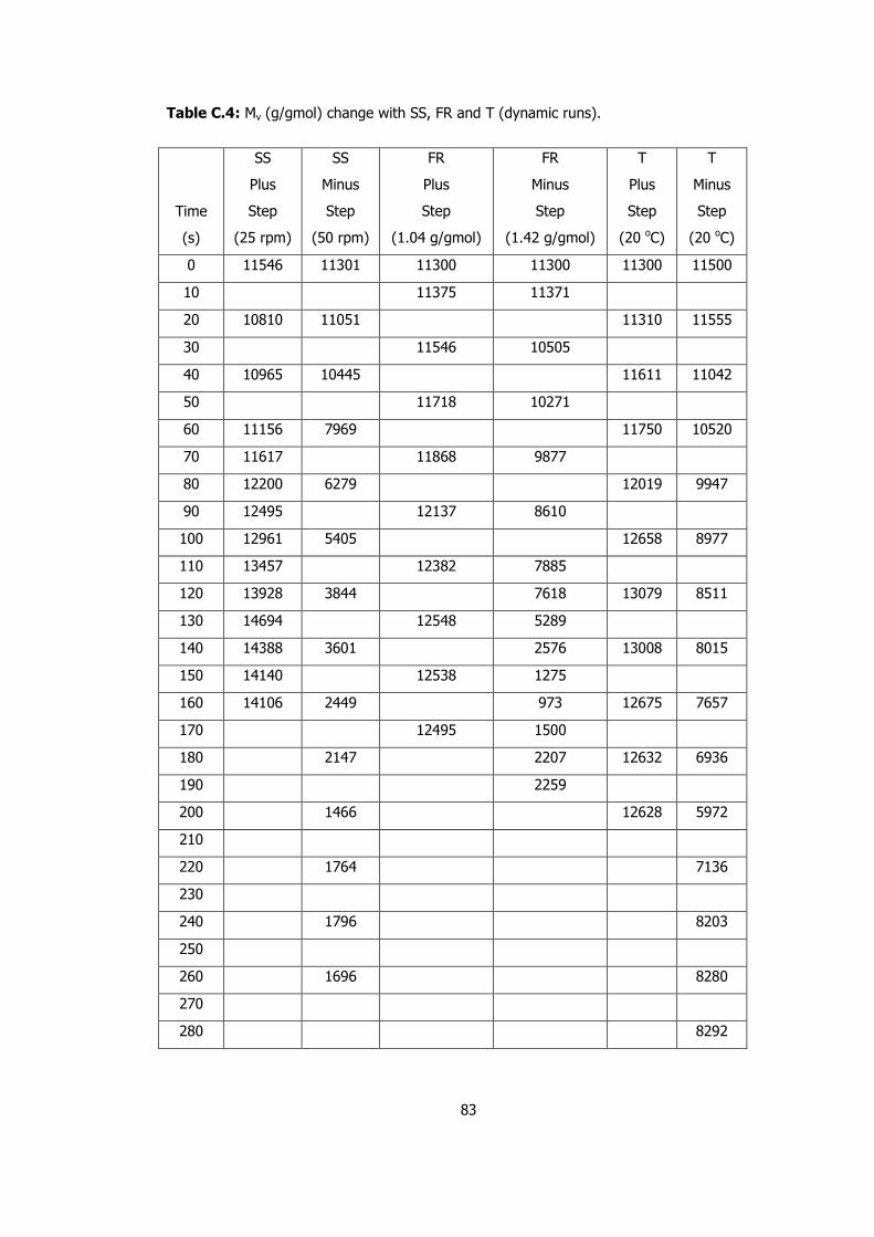
83
Table C.4: Mv (g/gmol) change with SS, FR and T (dynamic runs).
Time
(s)
SS
Plus
Step
(25 rpm)
SS
Minus
Step
(50 rpm)
FR
Plus
Step
(1.04 g/gmol)
FR
Minus
Step
(1.42 g/gmol)
T
Plus
Step
(20 oC)
T
Minus
Step
(20 oC)
0 11546 11301 11300 11300 11300 11500
10 11375 11371
20 10810 11051 11310 11555
30 11546 10505
40 10965 10445 11611 11042
50 11718 10271
60 11156 7969 11750 10520
70 11617 11868 9877
80 12200 6279 12019 9947
90 12495 12137 8610
100 12961 5405 12658 8977
110 13457 12382 7885
120 13928 3844 7618 13079 8511
130 14694 12548 5289
140 14388 3601 2576 13008 8015
150 14140 12538 1275
160 14106 2449 973 12675 7657
170 12495 1500
180 2147 2207 12632 6936
190 2259
200 1466 12628 5972
210
220 1764 7136
230
240 1796 8203
250
260 1696 8280
270
280 8292
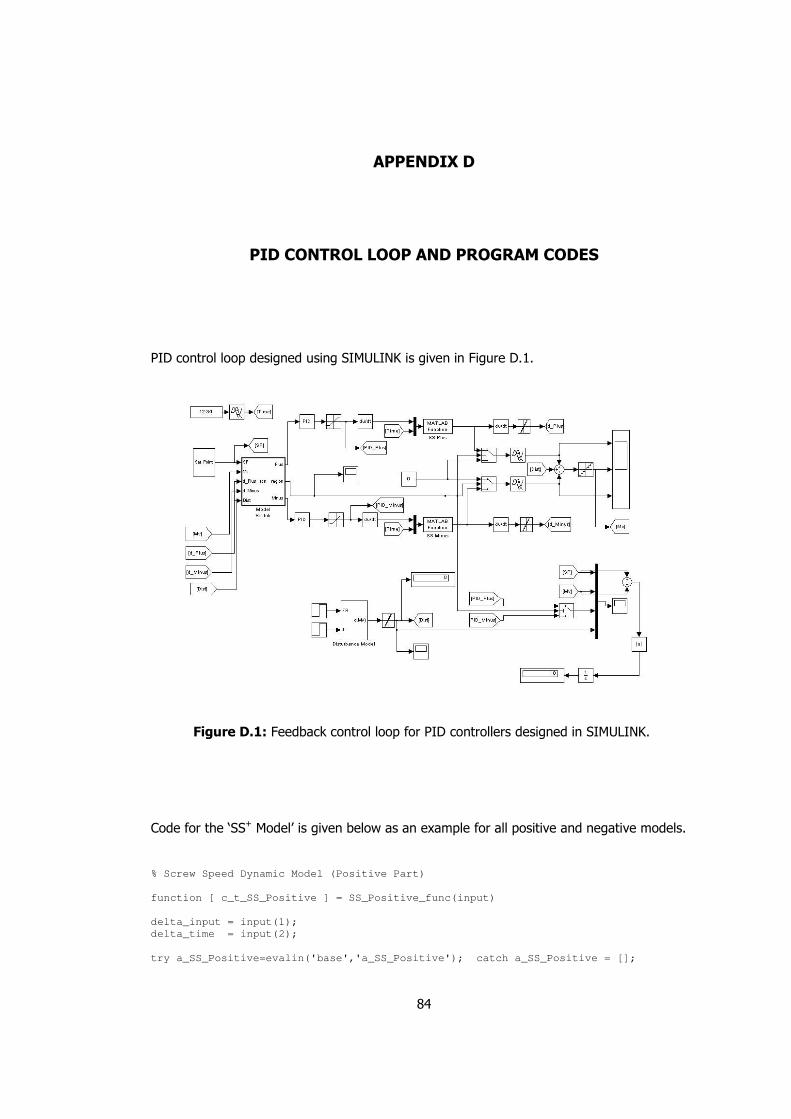
84
APPENDIX D
PID CONTROL LOOP AND PROGRAM CODES
PID control loop designed using SIMULINK is given in Figure D.1.
Figure D.1: Feedback control loop for PID controllers designed in SIMULINK.
Code for the ‘SS+ Model’ is given below as an example for all positive and negative models.
% Screw Speed Dynamic Model (Positive Part)
function [ c_t_SS_Positive ] = SS_Positive_func(input)
delta_input = input(1);
delta_time = input(2);
try a_SS_Positive=evalin('base','a_SS_Positive'); catch a_SS_Positive = [];
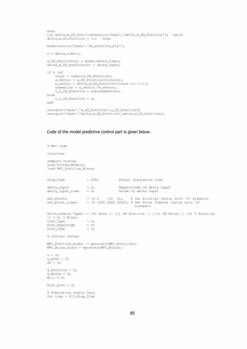
85
end;
try delta_m_SS_Positive=evalin('base','delta_m_SS_Positive'); catch
delta_m_SS_Positive = []; end;
model=evalin('base','SS_Positive_Fit');
n = delta_time+1;
a_SS_Positive(n) = model(delta_time);
delta_m_SS_Positive(n) = delta_input;
if n >=2
count = numel(a_SS_Positive);
a_vector = a_SS_Positive(2:count);
m_vector = delta_m_SS_Positive((count-1):-1:1);
summation = a_vector.*m_vector;
c_t_SS_Positive = sum(summation);
else
c_t_SS_Positive = 0;
end
assignin('base','a_SS_Positive',a_SS_Positive);
assignin('base','delta_m_SS_Positive',delta_m_SS_Positive);
Code of the model predictive control part is given below.
% MPC code
clc;clear
addpath Source;
load Fitted_Models;
load MPC_Positive_Minus;
Stop_Time = 500; %Total Simulation Time
delta_input = 0; %maginitude of delta input
delta_input_time = 0; %time of delta input
Set_Points = [0 0 -10 0]; % Set Point(s) vector with 'n' elements
Set_Point_times = [0 1000 2000 3000]; % Set Point Time(s) vector with 'n'
elements
%Disturbance Types -> (0) None || (1) FR Positive || (-1) FR Minus || (2) T Positive
|| (-2) T Minus
Dist_Type = 0;
Dist_Magnitude = 0;
Dist_Time = 0;
% Initial Values
MPC_Positive_state = mpcstate(MPC_Positive);
MPC_Minus_state = mpcstate(MPC_Minus);
u = 0;
u_prev = 0;
du = 0;
d_Positive = 0;
d_Minus = 0;
Mv_t = 0;
Dist_prev = 0;
% Simulation starts here
for time = 0:1:Stop_Time
86
for sp_detect = 1:numel(Set_Point_times) % Follow Set Points
if time == Set_Point_times(sp_detect)
Set_Point = Set_Points(sp_detect);
end
end
if not(Dist_Type == 0); % Disturbance Part
if time >= Dist_Time
dist_delta_time = time - Dist_Time;
Dist_delta_u = Dist_Magnitude - Dist_prev;
Mv_dist = disturbance_func(dist_delta_time,Dist_Type,Dist_delta_u);
Dist_prev = Dist_Magnitude;
else
Mv_dist = 0;
end
else
Mv_dist = 0;
end
region = region_select(d_Positive,d_Minus,Mv_t,Set_Point,Mv_dist);
switch region
case 0, % No models need to run
case 1, % SP Positive Region
clear minus_start_time
try Positive_start_time;
catch Positive_start_time = time;
end
u = mpcmove(MPC_Positive, MPC_Positive_state,Mv_t,Set_Point,[]);
du = u - u_prev;
Mv_t_prev = Mv_t;
delta_time = time - Positive_start_time;
Mv_t_Positive = SS_Positive_func([du delta_time]);
Mv_t = Mv_t_Positive + Mv_dist;
u_prev = u;
d_Positive = Mv_t - Mv_t_prev;
if abs(d_Positive) < 0.000001
d_Positive = 0;
end
if abs(Mv_t) < 0.1
Mv_t = 0;
end
assignin('base','Positive_start_time',Positive_start_time);
case -1, % SP Minus Region
clear Positive_start_time
try minus_start_time;
catch minus_start_time = time;
end
u = mpcmove(MPC_Minus,MPC_Minus_state,Mv_t,Set_Point,[]);
du = u - u_prev;
Mv_t_prev = Mv_t;
delta_time = time - minus_start_time;
Mv_t_minus = SS_Minus_func([du delta_time]);
87
Mv_t = Mv_t_minus + Mv_dist;
u_prev = u;
d_Minus = Mv_t - Mv_t_prev;
if abs(d_Minus) < 0.000001
d_Minus = 0;
end
if abs(Mv_t) < 0.1
Mv_t = 0;
end
assignin('base','minus_start_time',minus_start_time);
case 10, % Disturbance Positive Region
case -10, % Disturbance Minus Region
end
Mv_hist(time+1) = Mv_t;
Mv_dist_hist(time+1) = Mv_dist;
u_hist(time+1) = u;
du_hist(time+1) = du;
SP_hist(time+1) = Set_Point;
region_hist(time+1) = [region];
MPC_Dist_Response(time+1,:) = [time Set_Point Mv_dist Mv_t u];
end
disp 'finished'
subplot(2,1,1);plot(Mv_hist,'k');hold on;plot(SP_hist,':r');plot(Mv_dist_hist,'r');
subplot(2,1,2);plot(u_hist)
figure
plot(region_hist)
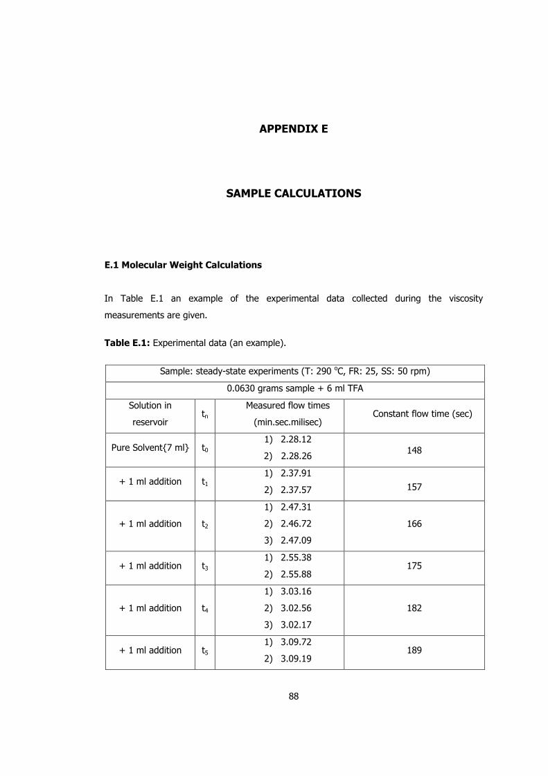
88
APPENDIX E
SAMPLE CALCULATIONS
E.1 Molecular Weight Calculations
In Table E.1 an example of the experimental data collected during the viscosity
measurements are given.
Table E.1: Experimental data (an example).
Sample: steady-state experiments (T: 290 oC, FR: 25, SS: 50 rpm)
0.0630 grams sample + 6 ml TFA
Solution in
reservoir tn
Measured flow times
(min.sec.milisec) Constant flow time (sec)
Pure Solvent{7 ml} t0 1) 2.28.12
2) 2.28.26 148
+ 1 ml addition t1 1) 2.37.91
2) 2.37.57
157
+ 1 ml addition t2
1) 2.47.31
2) 2.46.72
3) 2.47.09
166
+ 1 ml addition t3 1) 2.55.38
2) 2.55.88 175
+ 1 ml addition t4
1) 3.03.16
2) 3.02.56
3) 3.02.17
182
+ 1 ml addition t5 1) 3.09.72
2) 3.09.19 189
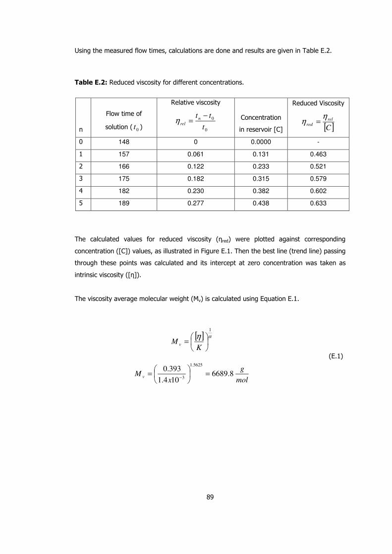
89
Using the measured flow times, calculations are done and results are given in Table E.2.
Table E.2: Reduced viscosity for different concentrations.
n
Flow time of
solution ( 0t )
Relative viscosity
0
0
t
ttn
rel
−=η Concentration
in reservoir [C]
Reduced Viscosity
[ ]C
rel
red
ηη =
0 148 0 0.0000 -
1 157 0.061 0.131 0.463
2 166 0.122 0.233 0.521
3 175 0.182 0.315 0.579
4 182 0.230 0.382 0.602
5 189 0.277 0.438 0.633
The calculated values for reduced viscosity (ηred) were plotted against corresponding
concentration ([C]) values, as illustrated in Figure E.1. Then the best line (trend line) passing
through these points was calculated and its intercept at zero concentration was taken as
intrinsic viscosity ([η]).
The viscosity average molecular weight (Mv) is calculated using Equation E.1.
[ ] αη1
=
KM v
mol
g
xM v 8.6689
104.1
393.05625.1
3=
=
−
(E.1)
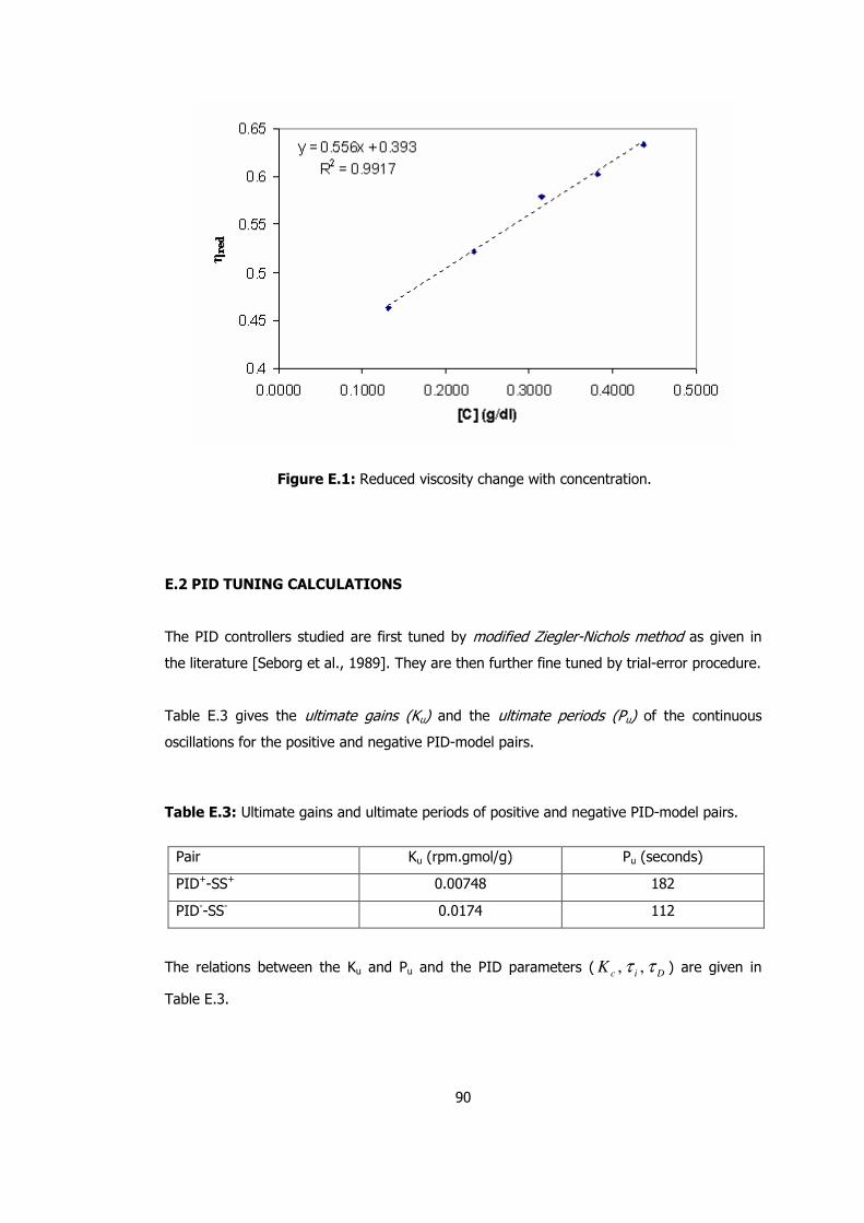
90
Figure E.1: Reduced viscosity change with concentration.
E.2 PID TUNING CALCULATIONS
The PID controllers studied are first tuned by modified Ziegler-Nichols method as given in
the literature [Seborg et al., 1989]. They are then further fine tuned by trial-error procedure.
Table E.3 gives the ultimate gains (Ku) and the ultimate periods (Pu) of the continuous
oscillations for the positive and negative PID-model pairs.
Table E.3: Ultimate gains and ultimate periods of positive and negative PID-model pairs.
Pair Ku (rpm.gmol/g) Pu (seconds)
PID+-SS+ 0.00748 182
PID--SS- 0.0174 112
The relations between the Ku and Pu and the PID parameters ( DicK ττ ,, ) are given in
Table E.3.

91
Table E.4: Original and modified Ziegler-Nichols settings for PID controllers [Seborg et al.,
1989].
cK iτ Dτ
Original (1/4 decay ratio) 0.6Ku Pu/2 Pu/8
Some Overshoot 0.33Ku Pu/2 Pu/3
No Overshoot 0.2Ku Pu/2 Pu/3