inferring gas consumption and pollution emission of ...dz220/cs671/6gasconsumption.pdf · inferring...
TRANSCRIPT
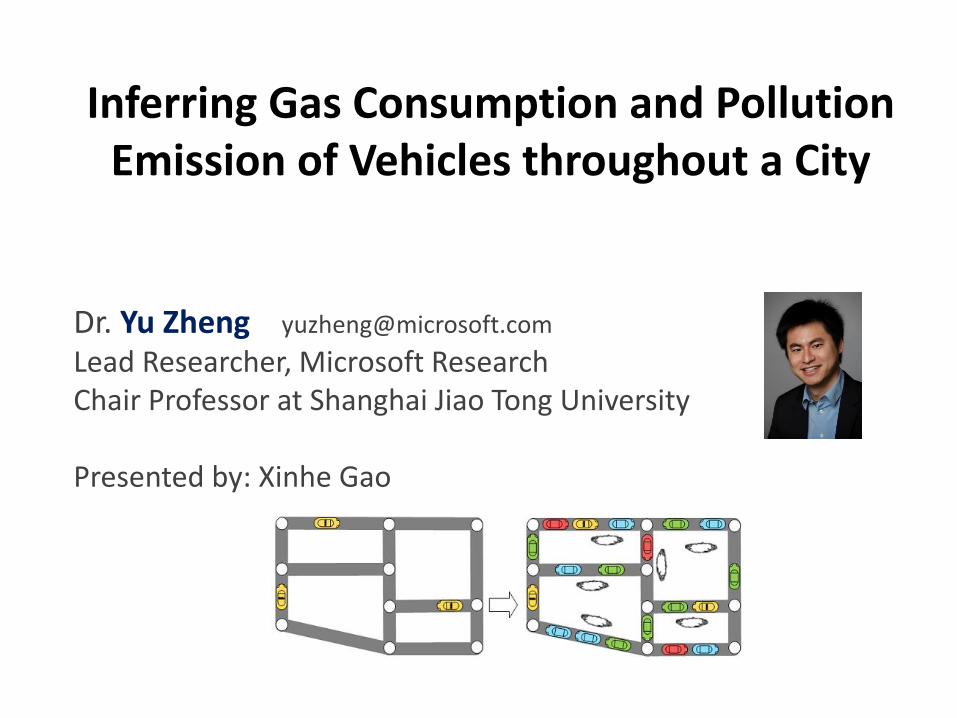
Inferring Gas Consumption and Pollution Emission of Vehicles throughout a City
Dr. Yu Zheng [email protected]
Lead Researcher, Microsoft Research Chair Professor at Shanghai Jiao Tong University
Presented by: Xinhe Gao
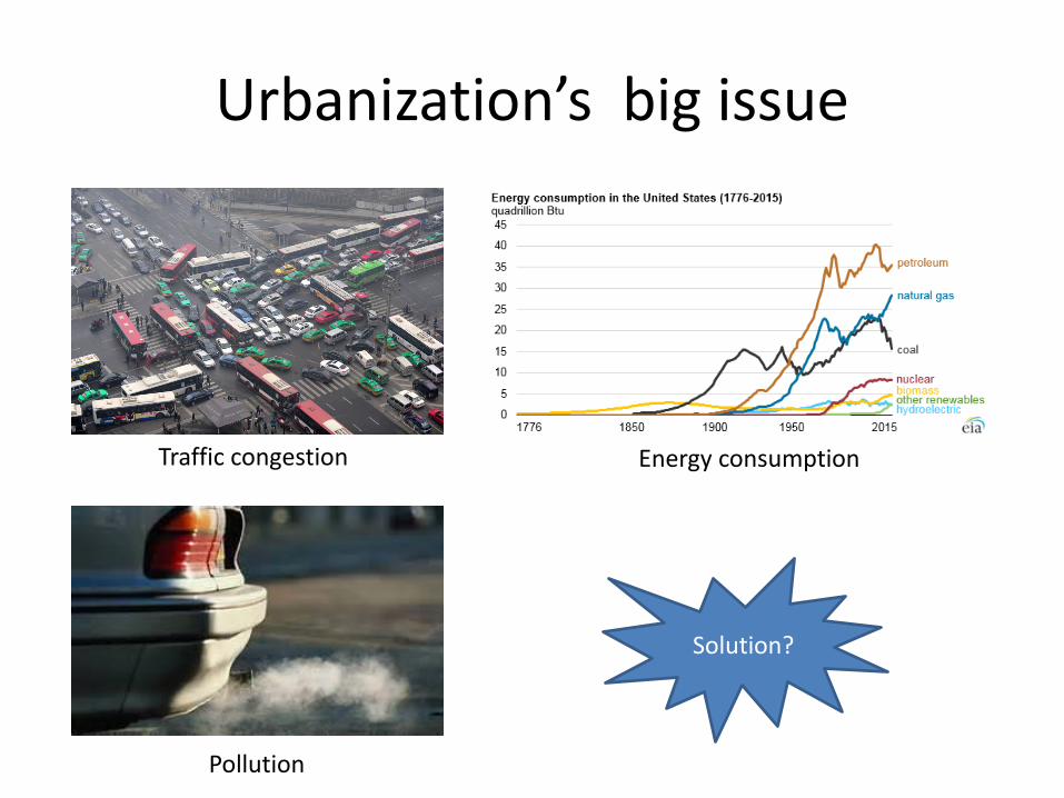
Urbanization’s big issue
Traffic congestion Energy consumption
Pollution
Solution?
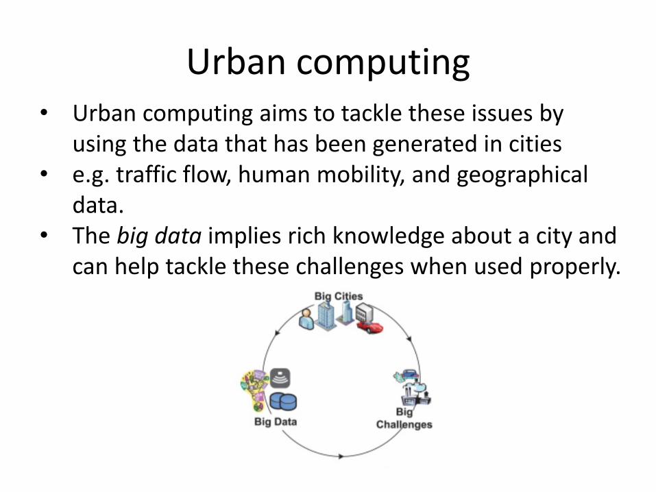
Urban computing• Urban computing aims to tackle these issues by
using the data that has been generated in cities • e.g. traffic flow, human mobility, and geographical
data. • The big data implies rich knowledge about a city and
can help tackle these challenges when used properly.
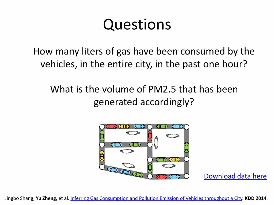
Questions
How many liters of gas have been consumed by the vehicles, in the entire city, in the past one hour?
What is the volume of PM2.5 that has been generated accordingly?
Download data here
Jingbo Shang, Yu Zheng, et al. Inferring Gas Consumption and Pollution Emission of Vehicles throughout a City. KDD 2014.
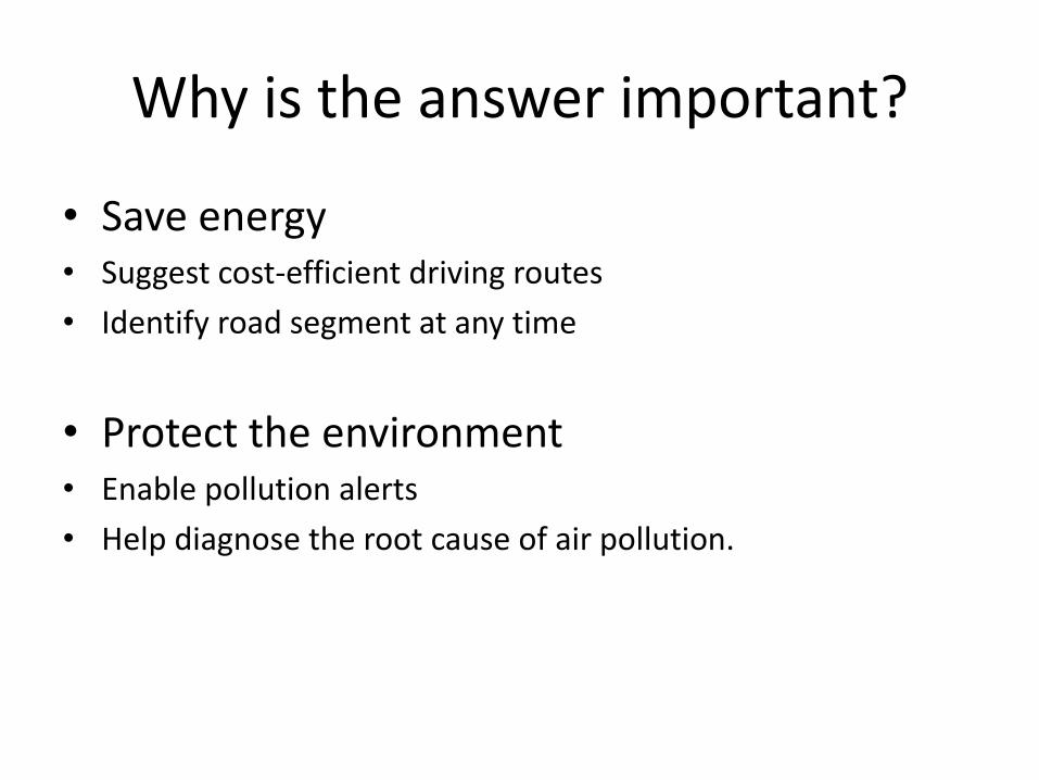
Why is the answer important?
• Save energy • Suggest cost-efficient driving routes
• Identify road segment at any time
• Protect the environment• Enable pollution alerts
• Help diagnose the root cause of air pollution.
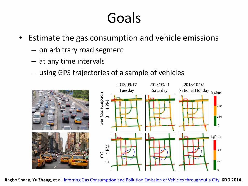
Goals• Estimate the gas consumption and vehicle emissions
– on arbitrary road segment
– at any time intervals
– using GPS trajectories of a sample of vehicles
0
150
240
kg/km
3 –
4 P
M
Gas
Con
sum
pti
on
2013/09/17
Tuesday
2013/09/21
Saturday
2013/10/02
National Holiday
0
kg/km
12
30
CO
3 –
4 P
M
Jingbo Shang, Yu Zheng, et al. Inferring Gas Consumption and Pollution Emission of Vehicles throughout a City. KDD 2014.

An Idea Solution
• Install sensors in each vehicle– Sensor monitoring gas consumption
– Sensor monitoring pollution emission
– GPS logger tracking the location
– Wireless communication module
• Mission impossible– Costly and obtrusive
– Privacy
impossible
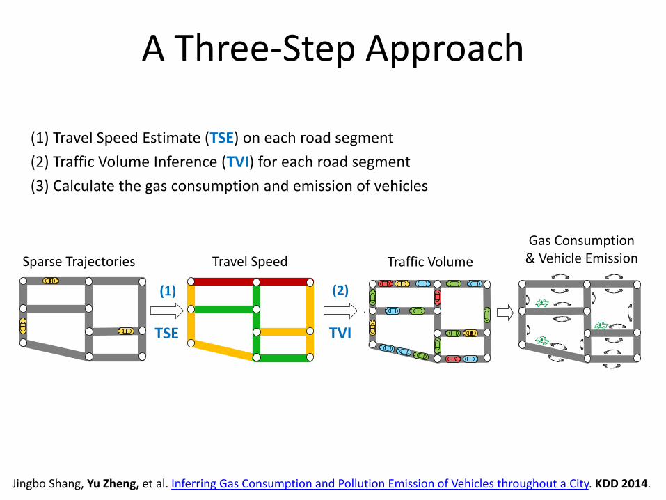
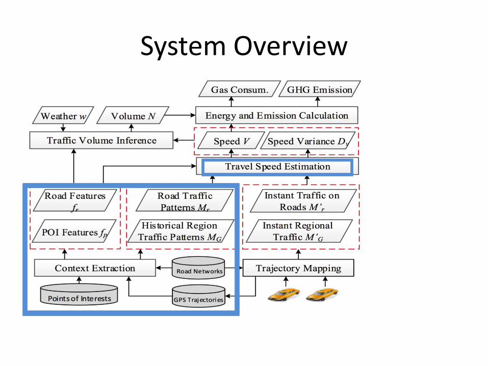
A Three-Step Approach
(1) Travel Speed Estimate (TSE) on each road segment
(2) Traffic Volume Inference (TVI) for each road segment
(3) Calculate the gas consumption and emission of vehicles
Jingbo Shang, Yu Zheng, et al. Inferring Gas Consumption and Pollution Emission of Vehicles throughout a City. KDD 2014.
Sparse Trajectories Travel Speed
Gas Consumption & Vehicle Emission
(1)
TSE
Traffic Volume
(2)
TVI
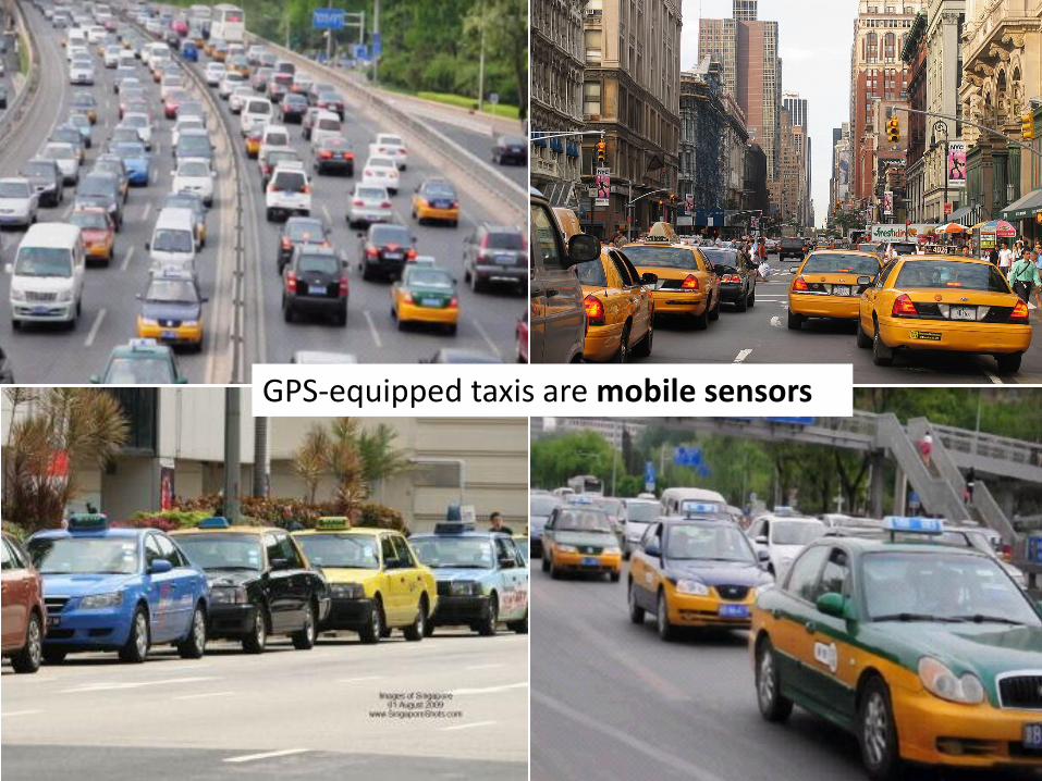
GPS-equipped taxis are mobile sensors
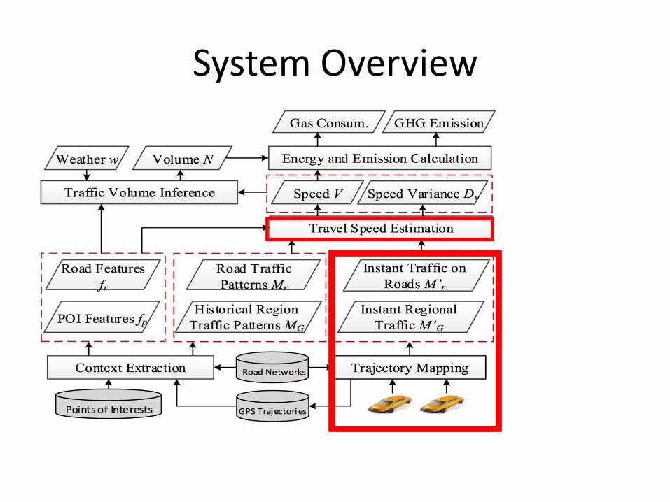
System Overview
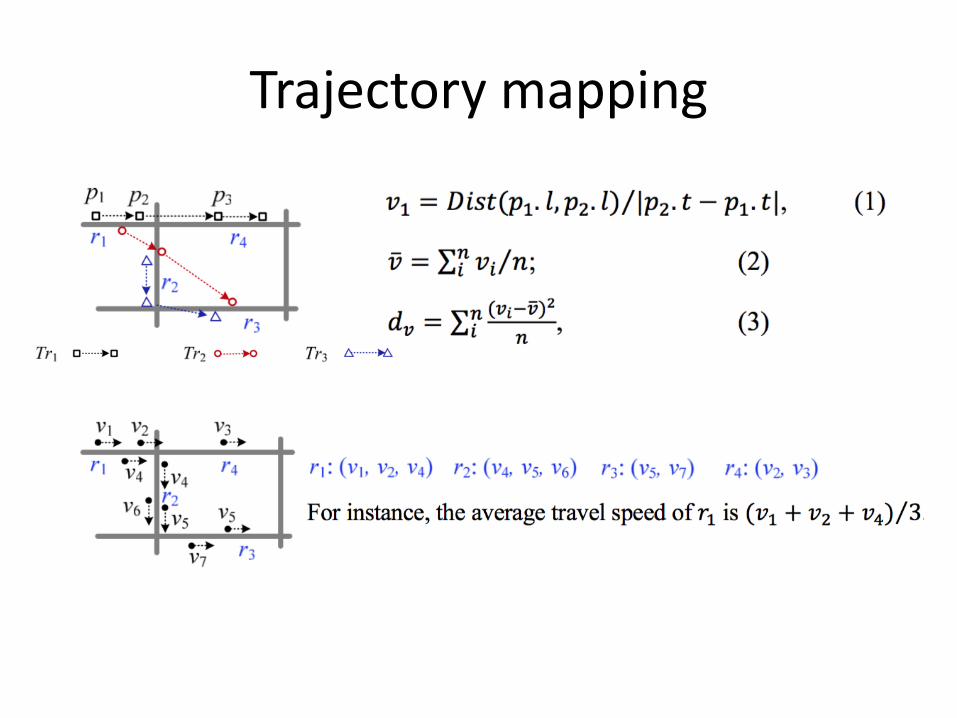
Trajectory mapping
System Overview
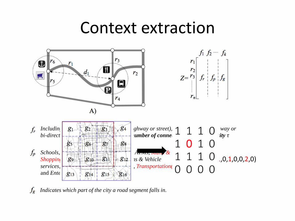
Context extraction
Including the road length, road level (highway or street), road direction (one way or
bi-direction), the number of lanes, the number of connections, and a tortuosity 𝜏
Schools, Companies & Offices, Banks & ATMs, Malls &
Shopping(1), Restaurants(1), Gas stations & Vehicle
services, Parking(1), Hotels, Residences, Transportation(2),
and Entertainment & Living Services.
(0,0,1,1,0,1,0,0,2,0)
Indicates which part of the city a road segment falls in.
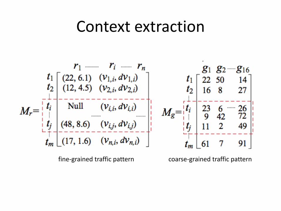
Context extraction
fine-grained traffic pattern coarse-grained traffic pattern
r1
d1 r2
r3
r4
r6
r5
r1
r2
rn
f1 f2 fk
Z
fr fp fg
Z
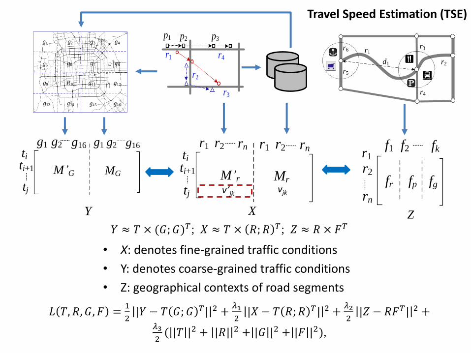
• X: denotes fine-grained traffic conditions
• Y: denotes coarse-grained traffic conditions
• Z: geographical contexts of road segments
𝐿 𝑇, 𝑅, 𝐺, 𝐹 =1
2|𝑌 − 𝑇 𝐺; 𝐺 𝑇| 2 +
𝜆1
2|𝑋 − 𝑇 𝑅; 𝑅 𝑇| 2 +
𝜆2
2|𝑍 − 𝑅𝐹𝑇| 2 +
𝜆3
2( |𝑇 |2 + |𝑅| 2 + |𝐺 |2 + |𝐹 |2),
Travel Speed Estimation (TSE)
𝑌 ≈ 𝑇 × (𝐺; 𝐺)𝑇; 𝑋 ≈ 𝑇 × 𝑅;𝑅 𝑇; 𝑍 ≈ 𝑅 × 𝐹𝑇XY
r2
Tr1
r3
r1
p1 p2
r4
p3
r2
r3
r1
v1 v2
r4
v3
v4 v4
v6 v5
v7
Tr2 Tr3
r1: (v1, v2, v4) r2: (v4, v5, v6) r3: (v5, v7) r4: (v2, v3)
v5
g1 g2 g3 g16ti
ti+1
219
42
00 0 0
6 17
0 0 0tj 0
014
g1 g2 g3
g16
g4
g5 g6 g7 g8
g9 R10 g11 g12
g13 g14 g15
g1 g2 g3 g16
t1 22
0420
35
110
0
0 0 0
16 8
0 00 15
0 31
0
tn
0
0
0
0
27
tj
ti
t2
0 0 0 7 0
MG=
=M G
r1 r2 rnti
ti+1
tj
M r Mr
r1 r2 rng1 g2 g16
ti
ti+1
tj
M G MG
g1 g2 g16
Y
v’jk vjk
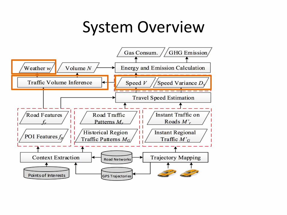
System Overview
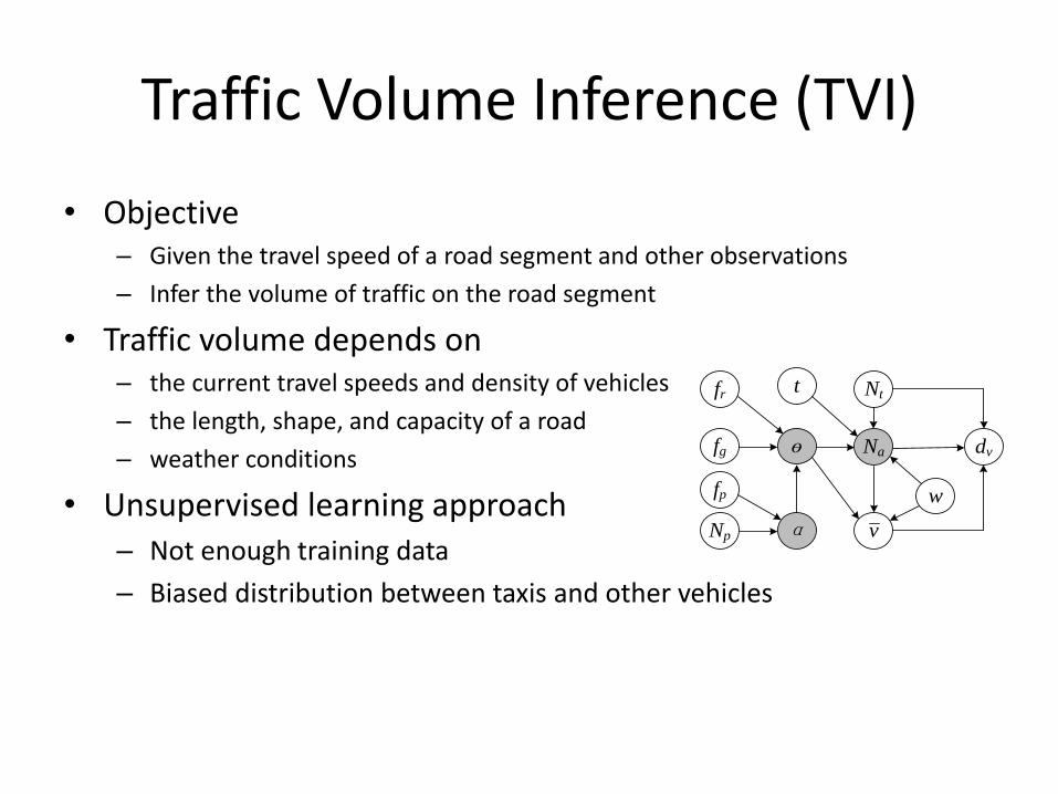
Traffic Volume Inference (TVI)
• Objective– Given the travel speed of a road segment and other observations
– Infer the volume of traffic on the road segment
• Traffic volume depends on– the current travel speeds and density of vehicles
– the length, shape, and capacity of a road
– weather conditions
• Unsupervised learning approach– Not enough training data
– Biased distribution between taxis and other vehicles
fp
fg
t Nt
ɵ Na
v
dv
fr
w
Np α
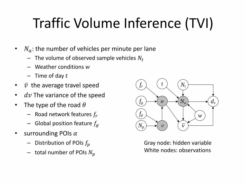
Traffic Volume Inference (TVI)
• 𝑁𝑎: the number of vehicles per minute per lane
– The volume of observed sample vehicles 𝑁𝑡– Weather conditions 𝑤
– Time of day 𝑡
• ҧ𝑣 the average travel speed
• 𝑑𝑣 The variance of the speed
• The type of the road 𝜃
– Road network features 𝑓𝑟
– Global position feature 𝑓𝑔
• surrounding POIs 𝛼
– Distribution of POIs 𝑓𝑝
– total number of POIs 𝑁𝑝
fp
fg
t Nt
ɵ Na
v
dv
fr
w
Np α
Gray node: hidden variable White nodes: observations
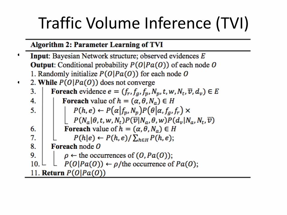
Traffic Volume Inference (TVI)
• EM algorithm
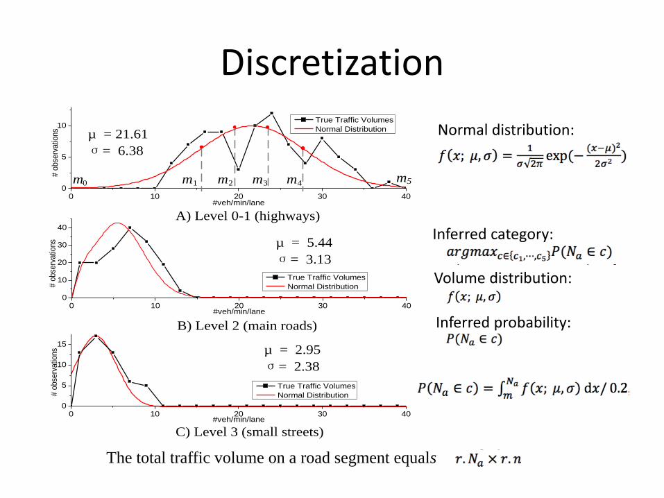
• Discretization of traffic volume– Recorded 358 video clips on 50 road segments at different time of day
– Manually count the traffic volume
– Fit a curve that reveals the distribution of the traffic volumes (for different levels)
– find a group of splitting points 𝑚0, 𝑚1, ⋯ ,𝑚5 that divide the traffic volume into five categories (𝑐1,𝑐2,…,𝑐5),
Discretization
0 10 20 30 400
5
10
# o
bse
rvatio
ns
#veh/min/lane
True Traffic Volumes
Normal Distributionµ = 21.61
σ= 6.38
0 10 20 30 400
10
20
30
40
# o
bse
rvatio
ns
#veh/min/lane
True Traffic Volumes
Normal Distribution
µ = 5.44
σ= 3.13
0 10 20 30 400
5
10
15
# o
bse
rvatio
ns
#veh/min/lane
True Traffic Volumes
Normal Distribution
µ = 2.95
σ= 2.38
A) Level 0-1 (highways)
B) Level 2 (main roads)
m1 m2 m3 m4m5 m 0
C) Level 3 (small streets)
Normal distribution:
Inferred category:
Volume distribution:
Inferred probability:
The total traffic volume on a road segment equals
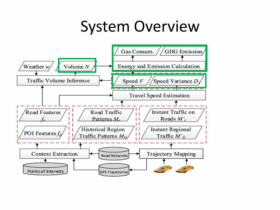
System Overview
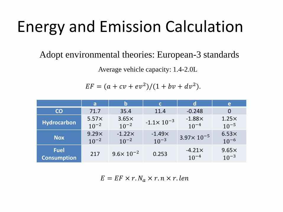
Energy and Emission Calculation
a b c d eCO 71.7 35.4 11.4 -0.248 0
Hydrocarbon5.57×10−2
3.65×10⁻²
-1.1× 10⁻³-1.88×10⁻⁴
1.25×10−5
Nox9.29×10−2
-1.22×10⁻²
-1.49×10⁻³
3.97× 10−56.53×10−6
Fuel Consumption
217 9.6× 10⁻² 0.253-4.21×10⁻⁴
9.65×10⁻³
𝐸𝐹 = (𝑎 + 𝑐𝑣 + 𝑒𝑣2)/(1 + 𝑏𝑣 + 𝑑𝑣2).
𝐸 = 𝐸𝐹 × 𝑟. 𝑁𝑎 × 𝑟. 𝑛 × 𝑟. 𝑙𝑒𝑛
Average vehicle capacity: 1.4-2.0L
Adopt environmental theories: European-3 standards
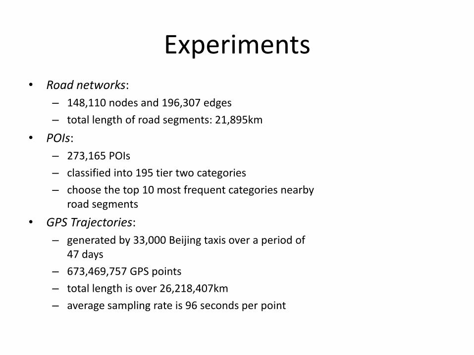
Experiments• Road networks:
– 148,110 nodes and 196,307 edges
– total length of road segments: 21,895km
• POIs:
– 273,165 POIs
– classified into 195 tier two categories
– choose the top 10 most frequent categories nearby road segments
• GPS Trajectories:
– generated by 33,000 Beijing taxis over a period of 47 days
– 673,469,757 GPS points
– total length is over 26,218,407km
– average sampling rate is 96 seconds per point
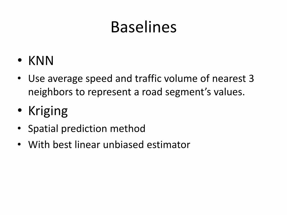
Baselines
• KNN• Use average speed and traffic volume of nearest 3
neighbors to represent a road segment’s values.
• Kriging• Spatial prediction method
• With best linear unbiased estimator
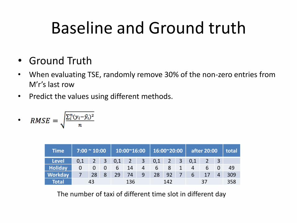
Baseline and Ground truth
• Ground Truth• When evaluating TSE, randomly remove 30% of the non-zero entries from
M’r’s last row
• Predict the values using different methods.
•
Time 7:00 ~ 10:00 10:00~16:00 16:00~20:00 after 20:00 total
Level 0,1 2 3 0,1 2 3 0,1 2 3 0,1 2 3Holiday 0 0 0 6 14 4 6 8 1 4 6 0 49
Workday 7 28 8 29 74 9 28 92 7 6 17 4 309Total 43 136 142 37 358
The number of taxi of different time slot in different day
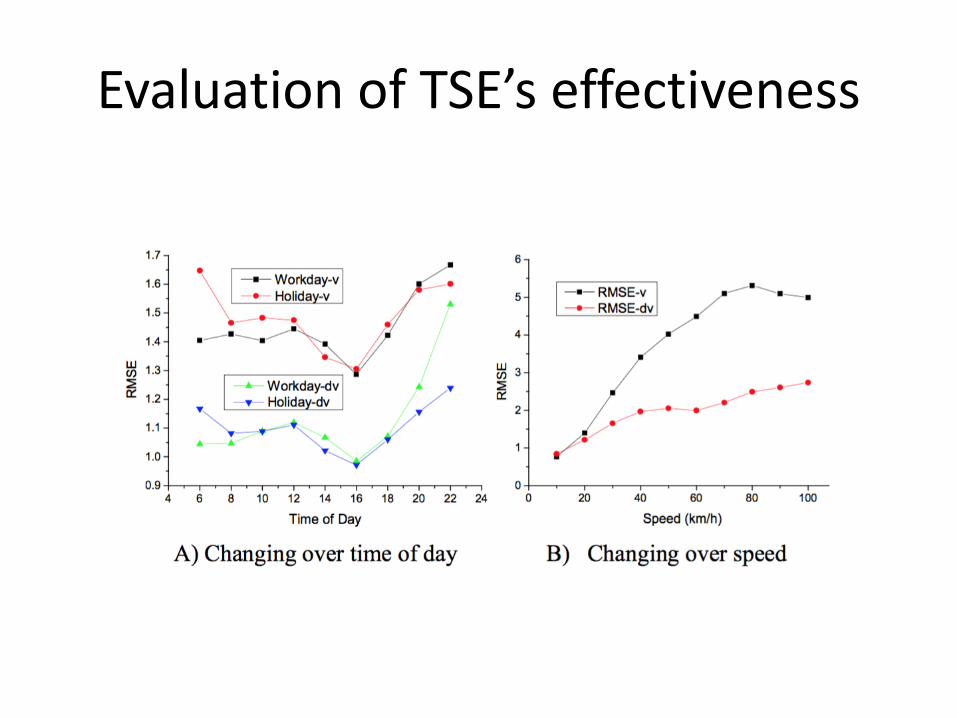
Evaluation of TSE’s effectiveness
Experiments
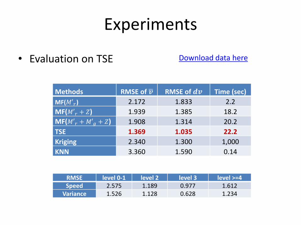
Methods RMSE of ഥ𝒗 RMSE of 𝒅𝒗 Time (sec)
MF(𝑀′𝑟) 2.172 1.833 2.2
MF(𝑀′𝑟 + 𝑍) 1.939 1.385 18.2
MF(𝑀′𝑟 +𝑀′𝑔 + 𝑍) 1.908 1.314 20.2
TSE 1.369 1.035 22.2
Kriging 2.340 1.300 1,000
KNN 3.360 1.590 0.14
• Evaluation on TSE
RMSE level 0-1 level 2 level 3 level >=4Speed 2.575 1.189 0.977 1.612
Variance 1.526 1.128 0.628 1.234
Download data here
Experiments
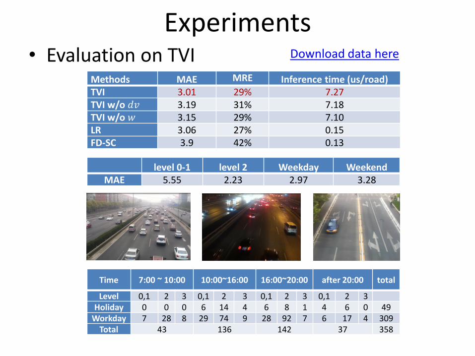
Methods MAE MRE Inference time (us/road)TVI 3.01 29% 7.27 TVI w/o 𝑑𝑣 3.19 31% 7.18TVI w/o 𝑤 3.15 29% 7.10LR 3.06 27% 0.15FD-SC 3.9 42% 0.13
• Evaluation on TVI
level 0-1 level 2 Weekday WeekendMAE 5.55 2.23 2.97 3.28
Download data here
Time 7:00 ~ 10:00 10:00~16:00 16:00~20:00 after 20:00 total
Level 0,1 2 3 0,1 2 3 0,1 2 3 0,1 2 3Holiday 0 0 0 6 14 4 6 8 1 4 6 0 49
Workday 7 28 8 29 74 9 28 92 7 6 17 4 309Total 43 136 142 37 358
Experiments
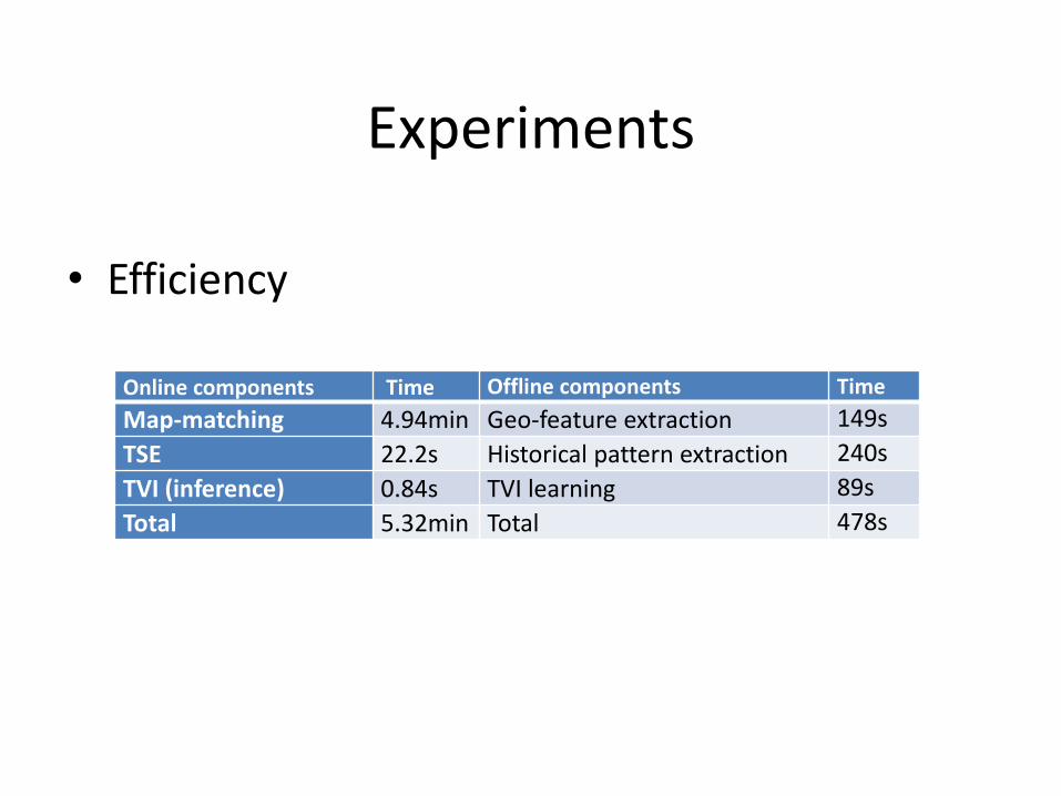
Online components Time Offline components Time
Map-matching 4.94min Geo-feature extraction 149s
TSE 22.2s Historical pattern extraction 240s
TVI (inference) 0.84s TVI learning 89s
Total 5.32min Total 478s
• Efficiency
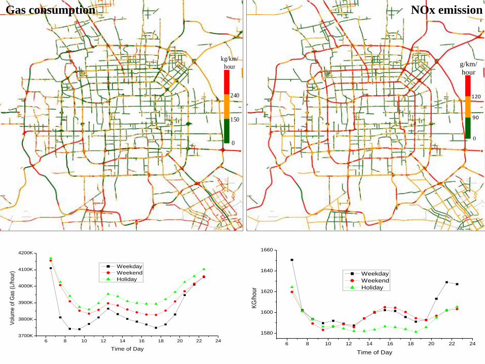
6 8 10 12 14 16 18 20 22 24
3700K
3800K
3900K
4000K
4100K
4200K
Volu
me o
f G
as
(L/h
our)
Time of Day
Weekday
Weekend
Holiday
6 8 10 12 14 16 18 20 22 24
1580
1600
1620
1640
1660K
G/h
our
Time of Day
Weekday
Weekend
Holiday
Gas consumption NOx emission
0
150
240
kg/km/
hour
90
120
g/km/
hour
0
Conclusion
• We can infer the citywide gas consumption and emission– Using a sample of vehicles
– in 8 minutes on a single machine
– With 70% accurate.
• Deal with data sparsity and data bias– Speed can be propagated while the volume cannot
– Unsupervised learning
– From a little labeled data distributions discretization

Q & A