inferring the size distribution of volcanic ash from iasi ... · inferring the size distribution of...

Inferring the size distribution of volcanic ash from IASImeasurements and optimal estimationLuke M. Western1, Peter N. Francis2, I. Matthew Watson1, and Shona Mackie3

1COMET, School of Earth Sciences, University of Bristol, Bristol, UK2Met Office, Exeter, UK3School of Earth Sciences, University of Bristol, Bristol, UK

Correspondence to: Luke M. Western ([email protected])

Abstract. This study demonstrates a method of retrieving the mass column loading and cloud-top pressure of a volcanic ash

cloud, together with the effective radius and spread of the ash particle size distribution, as well as the cloud top pressure of any

underlying water cloud, using an optimal estimation technique applied to Infrared Atmospheric Sounding Interferometer data.

Two shapes of particle size distribution are considered, a log-normal and a gamma distribution. Results show that it is viable

to retrieve a measure of the size distribution spread, namely the geometric standard deviation, when a log-normal distribution5

is assumed, whereas this is not the case for an assumed gamma distribution in terms of its effective variance. The volcanic

conditions under which the method works well are discussed, as are its shortcomings. The method is applied to two volcanic

eruptions: Eyjafjallajökull, Iceland using data from 6th May 2010 and Kasatochi, Alaska using data from 8th August 2008. The

results show that the retrieved geometric standard deviation of these ash clouds is spatially variable, and is generally similar

to what is assumed in many passive infrared remote sensing techniques. An abrupt change in the retrieved geometric standard10

deviation has been observed for the Eyjafjallajökull eruption along the trajectory of the ash cloud, and possible explanations

for this are discussed.

1 Introduction

Recent years have seen advancement in passive infrared remote sensing of volcanic ash. This was encouraged, at least in part,

by the widespread disruption caused during the 2010 eruption of Eyjafjallajökull, Iceland. Improvements in ash detection, (e.g.15

Clarisse et al., 2013; Mackie and Watson, 2014) and quantification of ash cloud properties (e.g. Francis et al., 2012; Pavolonis

et al., 2013) has allowed for corroboration (Millington et al., 2012), insertion (Wilkins et al., 2014) and assimilation (Pelley

et al., 2015) of remotely sensed data with atmospheric dispersion models to assist Volcanic Ash Advisory Centres (VAACs) in

preparing their advisories.

Despite progress in the field of volcanic ash remote sensing, large uncertainties are still apparent in many retrieval schemes20

(Corradini et al., 2008; Francis et al., 2012). In particular, little attention has been paid to the uncertainties encountered due

to uncertainty in particle size distribution, or the spread of the distribution when the shape of the particle size distribution

is known (Western et al., 2015). It is unlikely that the shape of the particle size distribution is known prior to retrieval and

conflicting data can emerge from in situ measurement from a single event (Turnbull et al., 2012). Issues surrounding airborne

1

Atmos. Meas. Tech. Discuss., doi:10.5194/amt-2016-92, 2016Manuscript under review for journal Atmos. Meas. Tech.Published: 4 May 2016c© Author(s) 2016. CC-BY 3.0 License.

in situ measurement are not unique to volcanic ash studies, see for example the discussion on measurement of meteorological

ice particles in Baumgardner et al. (2012).

This paper presents a method using the hyperspectral satellite sensor Infrared Atmospheric Sounding Interferometer to infer

an approximate size distribution of a volcanic ash cloud in terms of the moments of the size distribution and the limitations of

such a method. Some preliminary conclusions on particle size distribution are presented and compared to current knowledge.5

2 Infrared Atmospheric Sounding Interferometer

The Infrared Atmospheric Sounding Interferometer (IASI) is a nadir-looking Fourier transform spectrometer onboard the

Metop satellites (Clerbaux et al., 2009). The satellites have a polar sun-synchronous orbit with twice daily earth coverage and

a 50 km field of view at nadir with 4 footprints of 12 km in diameter over a swath width of ∼2200 km. The main advantage

of the IASI instrument is its unprecedented spectral coverage of 645 to 2760 cm−1, with spectral sampling of 0.25 cm−1 and10

apodized spectral resolution of 0.5 cm−1.

The IASI data used in the current study are acquired from the UK Centre for Environmental Data Archival (CEDA) after

processing at level 1c.

3 Method

The method employed here is, in essence, an amalgamation of the work by Francis et al. (2012) and Clarisse et al. (2010) with15

a measure of the spread of a particle size distribution added to the state vector used for the retrieval. Both these works, and the

current method, follow the work of Rodgers (2000) on inverse methods and optimal estimation. The approach taken, as applied

to volcanic ash retrieval, is briefly described in the following.

3.1 Optimal estimation

The basis of optimal estimation is the minimisation of the cost function defined by:20

−2lnP (x | y) = [y−F(x)]TS−1ε [y−F(x)] + [x−xa]TS−1

a [x−xa], (1)

where y is the observation, in this case the measured spectral radiances, F(x) is the simulated observation, in this case the

radiance calculated by some forward model, Sε contains the covariances between the observation and forward model, x is the

state vector, containing the parameters to be retrieved, xa is the vector containing the a priori estimates of the state vector and

Sa is the covariance between the state vector and the a priori estimates, i.e. the assumed uncertainty in knowledge of the state25

vector.

The minimisation is reached by an iterative method where the state vector is updated using Levenberg-Marquadt iterations

of the form:

xn+1 = xn + [(1 + γ)S−1a + KT

nS−1ε Kn]−1{KT

nS−1ε [y−F(xn)]−S−1

a [xn−xa]}, (2)

2


where γ is the Marquadt step parameter and K denotes the Jacobian matrix. In this case the scaling matrix has been chosen as

S−1a . The most likely solution of the state vector is reached when the gradient of the cost function equals zero, or when some

convergence criterion is reached. The gradient of the cost function is given as:

∇x{−2lnP (x | y)}=−KTS−1ε [y−F(x)] + S−1

a [x−xa], (3)

where∇x denotes the Fréchet derivative.5

3.2 Application to retrieval of volcanic ash

The state vector is chosen to encompass the retrievable parameters of an ash cloud, with elements consisting of the ash cloud

top pressure pash , the ash mass column loading L, the effective radius of the particle size distribution re and the spread

of the particle size distribution S, namely the geometric standard deviation σg or effective variance b of a log-normal or

gamma distribution respectively. This is a simplification of the cloud microphysical properties where assumptions on the ash10

composition, sphericity and conformation to an analytical particle size distribution are made. A log-normal distribution and

gamma distribution have both been suggested as representative particle size distributions for volcanic ash clouds (Wen and

Rose, 1994; Prata and Grant, 2001; Clarisse et al., 2010; Francis et al., 2012) and the retrieval method is run separately for both

size distributions. For a review of in situ measurements of airborne size distributions see Western et al. (2015). Ash clouds often

have underlying low-level stratus cloud present (see e.g. Prata and Prata, 2012, Fig. 7), which affects the upwelling radiation15

incident on the ash cloud. For this reason, a further element is included in the state vector, pcld, which is the cloud top pressure

of an underlying water cloud and where a value of pcld equal to the surface pressure corresponds to the case of an ash cloud

having no underlying water cloud. This underlying water cloud is assumed to be a blackbody. This is deemed a reasonable

approximation and simplifies the problem of scattering between multiple cloud layers (Watts et al., 2011).

The resultant representative state vector is therefore defined as:20

x =

pash

L

re

S

pcld

.

A log-normal distribution can be characterised by the probability density function:

n(r) =N0√

2πr lnσgexp

(−(

lnr− lnrg)2

2ln2σg

), (4)

where N0 is the total number of particles, r is the particle radius and rg is the geometric mean radius of the distribution.

3


The effective radius of a distribution of particles is defined as:

re =

∫∞0r3n(r)dr∫∞

0r3n(r)dr

, (5)

which for a log-normal distribution simplifies to:

re = rg exp(

52

ln2σg

). (6)

Conserving notation, and using b to represent the effective variance (Hansen and Travis, 1974), the probability density5

function for a gamma distribution is given as:

n(r) =N0(reb)

2b−1b

Γ( 1−2bb )

r1−3b

b exp(− r

reb

). (7)

A simple forward model is applied to simulate the IASI radiances (Prata, 1989), where the vector F(x) is made up of

modelled radiances Imodi for channel i:

Imodi (x) = (1− εi)Iup

i (pcld) + εiIoci (pash), (8)10

where Iupi is the modelled top of atmosphere upwelling radiance with no ash cloud present and Ioc

i is the modelled top of

atmosphere overcast radiances due to a blackbody at pressure pash. εi corresponds to the modelled spectral emissivity if an ash

cloud and is given by:

εi = 1− exp(−kext(re,S)L

cosθ

). (9)

kext is the scaled mass extinction coefficient (Chou et al., 1999) of a distribution of particles of size re and spread σg or b15

calculated using a Mie scattering routine (Bohren and Huffman, 2008) and θ is the satellite zenith angle.

Upwelling and overcast radiances are forward modelled using the fast radiative transfer code RTTOV (Hocking et al., 2013)

at the IASI pixel location. Surface and atmospheric data are taken from the European Centre for Medium-Range Weather

Forecasts (ECMWF) ERA-Interim Global Reanalysis data set (Dee et al., 2011) on 60 model levels. The ECMWF data are

interpolated linearly in both space and time to IASI pixel locations and acquisition times.20

It would be computationally impractical and would not greatly increase information content to use all IASI channels (Collard,

2007). For this reason a subset of 100 channels are selected in the range 700-1000 and 1100-1200 cm−1 every 4 cm−1, where

the ozone absorption band between 1000-1100 cm−1 has been excluded. These channels have been chosen as they are in an

atmospheric window sensitive to volcanic ash, incorporating the carbon dioxide absorption band to assist in the constraint of

pressure at ash cloud top.25

4


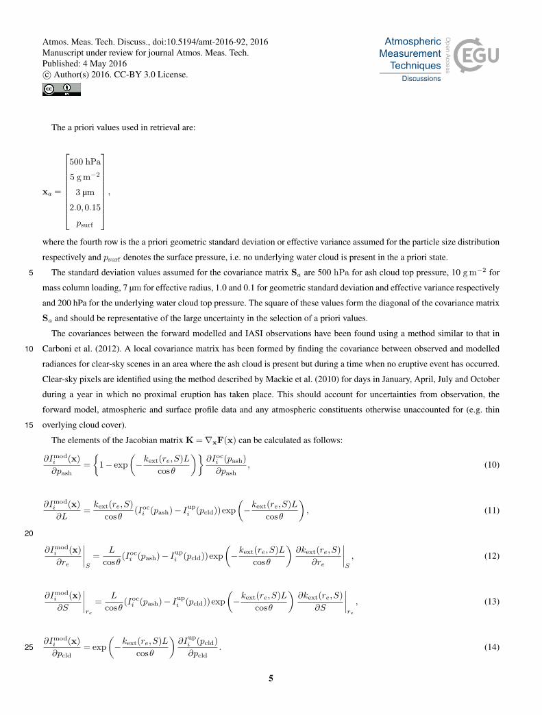
The a priori values used in retrieval are:

xa =

500 hPa

5 g m−2

3 µm

2.0,0.15

psurf

,

where the fourth row is the a priori geometric standard deviation or effective variance assumed for the particle size distribution

respectively and psurf denotes the surface pressure, i.e. no underlying water cloud is present in the a priori state.

The standard deviation values assumed for the covariance matrix Sa are 500 hPa for ash cloud top pressure, 10 g m−2 for5

mass column loading, 7 µm for effective radius, 1.0 and 0.1 for geometric standard deviation and effective variance respectively

and 200 hPa for the underlying water cloud top pressure. The square of these values form the diagonal of the covariance matrix

Sa and should be representative of the large uncertainty in the selection of a priori values.

The covariances between the forward modelled and IASI observations have been found using a method similar to that in

Carboni et al. (2012). A local covariance matrix has been formed by finding the covariance between observed and modelled10

radiances for clear-sky scenes in an area where the ash cloud is present but during a time when no eruptive event has occurred.

Clear-sky pixels are identified using the method described by Mackie et al. (2010) for days in January, April, July and October

during a year in which no proximal eruption has taken place. This should account for uncertainties from observation, the

forward model, atmospheric and surface profile data and any atmospheric constituents otherwise unaccounted for (e.g. thin

overlying cloud cover).15

The elements of the Jacobian matrix K =∇xF(x) can be calculated as follows:

∂Imodi (x)∂pash

={

1− exp(−kext(re,S)L

cosθ

)}∂Ioci (pash)∂pash

, (10)

∂Imodi (x)∂L

=kext(re,S)

cosθ(Ioci (pash)− Iup

i (pcld))exp(−kext(re,S)L

cosθ

), (11)

20

∂Imodi (x)∂re

∣∣∣∣S

=L



cosθ

)∂kext(re,S)

∂re

∣∣∣∣S

, (12)

∂Imodi (x)∂S

∣∣∣∣re

=L



cosθ

)∂kext(re,S)

∂S

∣∣∣∣re

, (13)

∂Imodi (x)∂pcld

= exp(−kext(re,S)L

cosθ

)∂Iupi (pcld)∂pcld

. (14)25

5


3.3 Information content of method

The information content of the retrieval in relation to the elements of the state vector can be represented by the averaging

kernel, given by:

A = (KTS−1ε K + S

−1

a )−1KTS−1ε K. (15)

This averaging kernel represents the sensitivity of the retrieval of the state vector elements to the physical state of what is to be5

retrieved.

The trace of the averaging kernel can be interpreted as the degrees of freedom for signal of the retrieval (DOF =∑aii).

This quantity is representative of the number of elements of the state vector that can be retrieved given a physical state,

albeit a continuous rather than discrete quantity. The degrees of freedom for a range of ash cloud properties for a log-normal

distribution and no underlying water cloud have been calculated and can be seen in Fig. 1 and for a gamma distribution in10

Fig. 2. The degrees of freedom for an ash cloud with an underlying water cloud can be seen in Fig. 3 and Fig. 4, where the

parameters describing the ash cloud are compared to a low-level underlying water cloud of varying altitude. For each grid,

two elements are varied across a range of likely encountered state vector values while the remaining state vector elements are

kept constant as their a priori values xa. Here an atmospheric profile was taken from 6th May 2010 (59◦N 12◦W) and Sε was

produced locally as described in the previous section. The refractive index used has been measured from ash collected during15

the 2010 Eyjafjallajökull eruption (Dan Peters, personal communication).

Figures 1 - 4 suggest that, in general, the retrieval of the spread of a log-normal particle size distribution has greater informa-

tion content than a gamma particle size distribution in relation to the physical state of the atmosphere and ash cloud due to the

greater number of physical states with high degrees of freedom. It is reasonable to conclude that one would be unable to detect

changes in the effective variance of a gamma distribution with much conviction in most volcanic remote sensing situations.20

However, a change in the geometric standard deviation of a log-normal particle size distribution appears to be detectable in

many conditions that would be of practical use in volcanic remote sensing applications. The limitation in the detection of a

change in size of particle size distribution with a large effective radius is known for broadband passive infrared retrievals (Wen

and Rose, 1994; Pavolonis et al., 2013) and this limitation is also apparent in hyperspectral retrievals due to the inherent single

scattering properties of volcanic ash. Other limitations appear to be when the ash cloud is of low altitude (pash & 700 hPa),25

when a size distribution spread is large, and when the column loading has very low or high values.

Figure 5 shows the fourth element of the diagonal of the averaging kernel, i.e. the element that describes the degree of

freedom for signal of the retrieval of spread for (a) a log-normal and (b) a gamma size distribution, for different values of

effective radius. The ash cloud is assumed to have its ash cloud top at the tropopause, no underlying water cloud and a mass

loading of 5 g m−2. These plots reinforce the difficulty in measuring a change in spread for large effective radii and a large30

value for spread.

It should be noted that the averaging kernel is strongly influenced by the choice of Sa. It follows that a change in choice for

the elements of Sa could change the interpreted degrees of freedom for signal. Airborne volcanic ash has not been measured as

having a gamma size distribution in situ, whereas a log-normal distribution has been measured (Farlow et al., 1981; Schumann

6


et al., 2011; Johnson et al., 2012). Other studies may have used a gamma size distribution due to it being measured for other

volcanic species, such as sulphuric acid (e.g. Brogniez et al., 1997). For this reason only a log-normal particle size distribution

is used hereafter in the retrieval scheme to approximate the spread of the ash particle size distribution.

3.4 Optical properties of ash

The mass extinction coefficient is known to vary with the refractive index and spread of a distribution of particles (Jennings5

et al., 1979; Bohren and Huffman, 2008). This means that mass extinction is both wavelength and size distribution dependent,

which leads to a unique spectral signal when a broad range of wavelengths is used. The dependence can be quite clearly seen

for a log-normal distribution in Fig. 6, where geometric standard deviations between σg = 1.5− 3.0 are shown at wavelengths

of 13.4, 12.0, 10.8 and 8.7 µm using refractive indices for ash from the 2010 Eyjafjallajökull eruption (Dan Peters, personal

communication). This serves as the physical basis as to how a unique size distribution can be retrieved over a broad spectral10

range. This uniqueness is much less pronounced for a gamma distribution (Fig. 7), where a change in effective variance b is

much less distinguishable at most effective radii and relevant wavelengths, and hence fewer degrees of freedom. For Figs. 6

and 7 the spreads of size distributions are intended to be representative of those likely to occur in nature for volcanic aerosols.

4 Case studies

4.1 2010 Eyjafjallajökull eruption15

The April - May 2010 Eyjafjallajökull eruption in Iceland was well observed and has been extensively studied from a variety

of perspectives (e.g. Schumann et al., 2011; Gudmundsson et al., 2012; Prata and Prata, 2012; Spinetti et al., 2013). Since

the eruption a refractive index data set has been measured for ash collected in Iceland on 17th April 2010 (Dan Peters, per-

sonal communication) and the bulk density of the very fine ash deposited in the period 4-8th May has been determined to be

2738 kg m−3 (Bonadonna et al., 2011). These data would most likely be unavailable during any real-time monitoring of an20

eruption but is convenient for post-eruptive analysis. The particle size distribution has been shown to be log-normal through in

situ aircraft measurement (Schumann et al., 2011; Johnson et al., 2012), although discrepancies in the spread of the distribution

exist (Turnbull et al., 2012).

Figure 8 shows the brightness temperature difference of an IASI image, with an overpass at 21:50 UTC on 6th May 2010. The

brightness temperature difference is the difference between brightness temperatures at 10.8 and 12.0 µm (926 and 833.5 cm−125

respectively), BTD =BT926−BT833.5. Volcanic ash generally gives a negative BTD while water or ice cloud generally has

a positive BTD (Prata, 1989).

4.2 2008 Kasatochi eruption

Kasatochi is a volcano located in the central Aleutian Islands of Alaska. Between 7 - 8th August 2008 it underwent a violent

eruption where the majority of the ash was deposited over sea. There is little available compositional information on the distal30

7


ash from the eruption, however it can be inferred from proximal juvenile material that the eruption was andesitic in composition

(Waythomas et al., 2010) and an andesitic refractive index (Pollack et al., 1973) has been used for the retrieval. Although the

assumption of refractive index is necessary, it is expected that the detection (Mackie et al., 2014) and retrieval (Clarisse et al.,

2010; Francis et al., 2012) is sensitive to the refractive index chosen. The ash bulk density is assumed to be similar to other

andesitic eruptions and a value of 2300 kg m−3 has been used (Bonadonna and Phillips, 2003). The size distribution of the5

volcanic ash is an unknown and a log-normal particle size distribution has been chosen as the most suitable.

The eruption plume contained a large SO2 loading (Prata et al., 2010) and can be seen by the large ν1 absorption band

present around 1152 cm−1 in Fig. 9. The forward model used in the retrieval, Eq. (8), does not account for the presence of SO2

in the ash cloud. It was therefore decided to only use channels in the range 700-1000 cm−1 for the retrieval from this eruption.

The brightness temperature difference of an IASI image from 8th August 2008, with an overpass at 21:25 UTC, can be seen10

in Fig. 10.

4.3 Detection of ash

For this work, pixels containing volcanic ash have been identified using a probabilistic detection scheme (Mackie and Watson,

2014), whereby the probability with which a pixel is associated with each of three states, clear, cloud and ash, is calculated.

The states are assumed to be mutually exclusive and so the probabilities for any one pixel sum to unity. Mixed cloud-ash pixels15

are likely to correspond to elevated probabilities for both cloud and ash, while clear pixels and ‘pure’ ash and cloud pixels are

likely to correspond to probabilities approaching either zero or unity for each state. For the purposes of this work, pixels with

a calculated probability for ash exceeding 0.2 were deemed to contain ash, and all other pixels were deemed ash free.

5 Results and Discussion

5.1 Retrieved properties20

The properties of ash clouds, from the 2010 eruption of Eyjafjallajökull on 6th May and 2008 eruption of Kasatochi on 8th

August have been retrieved using the method described in section 3 and the IASI sensor. The retrieved state vector values

of the ash cloud can be seen in Figs. 11 and 12 for Eyjafjallajökull on 6th May and Kasatochi on 8th August repectively.

The underlying cloud top pressure is not shown as it is not a parameter that describes the ash cloud itself, rather a nuisance

parameter of necessity to better describe the system. The effects of including an underlying water cloud in the retrieval is an25

interesting problem in itself as changes in the upwelling radiation incident on the ash cloud will affect retrieved parameters.

The inclusion of a non-clear-sky atmosphere to model upwelling radiation during retrieval may be important for improvements

to retrievals using both broadband and hyperspectral sensors.

8


5.2 2010 Eyjafjallajökull eruption retrieval

A histogram showing the retrieved geometric standard deviation values from Fig. 11(a) can be seen in Fig. 13(a). Two modes

are apparent around σg = 2.0 and 2.8, the implications of which are discussed in the section 5.4.

5.3 2008 Kasatochi eruption retrieval

Unlike the 2010 eruption of Eyjafjallajökull, no refractive index data are available for the 2008 Kasatochi eruption and the5

composition has been inferred from juvenile material deposited mainly through pyroclastic density currents, which may result

an incorrect assumption for the refractive index. Similarly, no in situ data are available on the shape of the particle size

distribution of the ash. The size distribution conforming to a log-normal shape is merely an assumption to which the entire ash

cloud may not conform.

The geometric standard deviation values for Kasatochi from Fig. 12(a) are shown in Fig. 13(b), which has a single mode10

present around σg = 2.1.

5.4 Discussion

Particle sedimentation from an ash cloud is somewhat complex, where particle settling and vertical transfer is more sophisti-

cated than the Lagrangian dynamics of individual particle settling (Carazzo and Jellinek, 2013). Diffuse convection can lead

to such phenomena as particle layering and fingering during sedimentation (Green, 1987; Osborn et al., 1995; Carazzo and15

Jellinek, 2013; Costa et al., 2013). As a result, it seems reasonable that the size distribution of an ash cloud, in terms of spread,

does not remain temporally or spatially constant in a heterogenous atmosphere.

The retrieved geometric standard deviation for Eyjafjallajökull from 6th May 2010 has a mode around 2.0, in line with

current assumed geometric standard values (e.g. Clarisse et al., 2010), and also consistent with values derived from in situ

sampling during the eruption, where geometric standard deviation values in the range 1.8 - 2.5 were measured (Turnbull20

et al., 2012). A larger mode around 2.8 is also present, a value greater than those observed by in situ measurement during the

eruption. The geometric standard deviation appears to get smaller as the ash cloud progresses. In situ measurement during the

2010 Eyjafjallajökull eruption was carried out in areas of relatively low mass concentration. These ash clouds were generally

more aged than that shown in Fig. 11 (Schumann et al., 2011; Johnson et al., 2012). If the geometric standard deviation of the

particle size distribution is indeed changing along the trajectory, it is therefore of little surprise that in situ observations differ25

from those retrieved in Fig. 13(a).

There is a narrowing in the spread of the size distribution of the Eyjafjallajökull ash cloud at around 14◦W 55◦N and

westward from here. This appears to match a change in the altitude of the ash cloud. This could be for a variety of reasons and

some of the possibilities are suggested.

(1) As previously mentioned, atmospheric sorting can lead to layering of particles. Here the lower altitude ash cloud farther30

along the trajectory could be a lower altitude layer containing finer particles after such sorting effects have taken place.

9


(2) It is known from Fig. 1 that a range of factors can affect the sensitivity of the retrieval scheme. It may be that the retrieval

is less sensitive as this ash cloud top is of lower altitude.

(3) Closer to the volcano the ash cloud may be less well separated from other volcanogenic emissions. Absorption due to

SO2 has been assumed to be negligible and thus not affecting Eq. (8). If this is not the case then it may cause the retrieval to

converge on a non-representative solution.5

(4) The eruption intensity varied substantially throughout the course of the day on 6th May 2010 (Ripepe et al., 2013). A

change in the spread of the size distribution may therefore be a result of a change in eruption intensity and dynamics.

Kasatochi shows a mode for the geometric standard deviation around 2.1. As no in situ observations are available for this

eruption, it is difficult to validate or criticise the retrieval. However, the geometric standard deviation values shown in Fig. 13(b)

are generally similar to log-normal size distributions measured through in situ measurement (Farlow et al., 1981; Schumann10

et al., 2011; Johnson et al., 2012).

In all circumstances pixels are assumed to be ash-filled and therefore retrievals close to the volcano, where lateral spreading

of the ash cloud may have had less time to take effect, or on the peripheries of the ash cloud, may result in an unrepresentative

retrieval due to the condition of ash-filled pixels no longer being fulfilled. The large footprint of IASI may make it particularly

susceptible to this effect. An ash cloud mixed with water cloud or ice particles, rather than a separate underlying water cloud,15

is not described by Eq. (8) and would lead to an unrepresentative retrieval. Over a long time period, it would be unsurprising

for the size distribution of volcanic ash to tend to some standard form due to atmospheric sorting.

6 Conclusions

This study has shown that, under certain conditions, it is possible to infer the particle size distribution of volcanic ash clouds,

in terms of the moments of a log-normal size distribution, using the IASI sensor. The conditions in which the retrieval method20

can reliably retrieve all state vector elements and where the method has its shortcomings are shown in Figs. 1 and 3 for a

log-normal particle size distribution and Fig. 2 and 4 for a gamma size distribution. The study suggests that this method is

unable to retrieve a change in the spread of a gamma distribution but is able to detect a change in the spread of a log-normal

distribution, which literature suggests is a more appropriate choice of distribution, in many volcanic conditions.

The retrieval of the geometric standard deviation of a log-normal particle size distribution from the April-May 2010 eruption25

of Eyjafjallajökull, Iceland suggests that the spread of the particle size distribution is spatially variable and, in places, may be

larger than what has previously been observed through in situ measurement by aircraft and what is assumed in many current

volcanic ash retrieval methods. However, it can also be seen that for much of the ash cloud the geometric standard deviation is

much inline with current assumptions made in many retrieval schemes. For the 2008 eruption of Kasatochi, Alaska the retrieved

geometric standard deviation values for the majority of pixels are close to those generally assumed in the literature. It is shown30

that the size distribution of the particles is spatially variant within an ash cloud, an issue which is generally unaccounted for

in many passive infrared remote sensing techniques, and the geometric standard deviation of the particle size distribution may

change over the lifetime of the eruption.

10


Validation of the retrieval method is difficult due to the sparsity of information on ash particle size distributions within the

ash cloud, where currently measurements have generally been taken on the peripheries of a dilute cloud or after a lengthy

residence time in the atmosphere.

For efficient, real-time retrieval methods, such as Prata and Prata (2012), this method may prove beneficial by helping to

approximate the spread of the size distribution and as a comparison to other retrieval techniques where a fixed spread in the5

size distribution is assumed.

Acknowledgements. The European Centre for Medium-Range Weather Forecasts and EUMETSAT are acknowledged for providing atmo-

spheric and satellite data for this study. Roger Saunders, Franco Marenco and Kate Wilkins are thanked for their helpful comments on the

manuscript. This work was supported by grant number Ne/K007912/1, a NERC Met Office CASE studentship.

11


References

Baumgardner, D., Avallone, L., Bansemer, A., Borrmann, S., Brown, P., Bundke, U., Chuang, P., Cziczo, D., Field, P., Gallagher, M., et al.:

In situ, airborne instrumentation: Addressing and solving measurement problems in ice clouds, 2012.

Bohren, C. F. and Huffman, D. R.: Absorption and scattering of light by small particles, John Wiley & Sons, 2008.

Bonadonna, C. and Phillips, J. C.: Sedimentation from strong volcanic plumes, Journal of Geophysical Research: Solid Earth (1978–2012),5

108, 2003.

Bonadonna, C., Genco, R., Gouhier, M., Pistolesi, M., Cioni, R., Alfano, F., Hoskuldsson, A., and Ripepe, M.: Tephra sedimentation during

the 2010 Eyjafjallajökull eruption (Iceland) from deposit, radar, and satellite observations, Journal of Geophysical Research: Solid Earth

(1978–2012), 116, 2011.

Brogniez, C., Lenoble, J., Ramananahérisoa, R., Fricke, K., Shettle, E., Hoppel, K., Bevilacqua, R., Hornstein, J., Lumpe, J., Fromm, M.,10

et al.: Second European Stratospheric Arctic and Midlatitude Experiment campaign: Correlative measurements of aerosol in the northern

polar atmosphere, Journal of Geophysical Research: Atmospheres, 102, 1489–1494, 1997.

Carazzo, G. and Jellinek, A.: Particle sedimentation and diffusive convection in volcanic ash-clouds, Journal of Geophysical Research: Solid

Earth, 118, 1420–1437, 2013.

Carboni, E., Grainger, R., Walker, J., Dudhia, A., and Siddans, R.: A new scheme for sulphur dioxide retrieval from IASI measurements:15

application to the Eyjafjallajökull eruption of April and May 2010, Atmospheric Chemistry and Physics, 12, 11 417–11 434, 2012.

Chou, M.-D., Lee, K.-T., Tsay, S.-C., and Fu, Q.: Parameterization for cloud longwave scattering for use in atmospheric models, Journal of

climate, 12, 159–169, 1999.

Clarisse, L., Hurtmans, D., Prata, A. J., Karagulian, F., Clerbaux, C., De Mazière, M., and Coheur, P.-F.: Retrieving radius, concentration,

optical depth, and mass of different types of aerosols from high-resolution infrared nadir spectra, Applied optics, 49, 3713–3722, 2010.20

Clarisse, L., Coheur, P.-F., Prata, F., Hadji-Lazaro, J., Hurtmans, D., and Clerbaux, C.: A unified approach to infrared aerosol remote sensing

and type specification., Atmospheric Chemistry & Physics, 13, 2013.

Clerbaux, C., Boynard, A., Clarisse, L., George, M., Hadji-Lazaro, J., Herbin, H., Hurtmans, D., Pommier, M., Razavi, A., Turquety, S.,

et al.: Monitoring of atmospheric composition using the thermal infrared IASI/MetOp sounder, Atmospheric chemistry and physics, 9,

6041–6054, 2009.25

Collard, A.: Selection of IASI channels for use in numerical weather prediction, Quarterly Journal of the Royal Meteorological Society, 133,

1977–1991, 2007.

Corradini, S., Spinetti, C., Carboni, E., Tirelli, C., Buongiorno, M. F., Pugnahi, S., and Gangale, G.: Mt. Etna tropospheric ash retrieval

and sensitivity analysis using Moderate Resolution Imaging Spectroradiometer measurements, Journal of Applied Remote Sensing, 2,

023 550–023 550, 2008.30

Costa, A., Folch, A., and Macedonio, G.: Density-driven transport in the umbrella region of volcanic clouds: Implications for tephra disper-

sion models, Geophysical Research Letters, 40, 4823–4827, 2013.

Dee, D., Uppala, S., Simmons, A., Berrisford, P., Poli, P., Kobayashi, S., Andrae, U., Balmaseda, M., Balsamo, G., Bauer, P., et al.: The

ERA-Interim reanalysis: Configuration and performance of the data assimilation system, Quarterly Journal of the Royal Meteorological

Society, 137, 553–597, 2011.35

Farlow, N. H., Oberbeck, V. R., Snetsinger, K. G., Ferry, G. V., Polkowski, G., and Hayes, D. M.: Size distributions and mineralogy of ash

particles in the stratosphere from eruptions of Mount St. Helens, Science, 211, 832–834, 1981.

12


Francis, P. N., Cooke, M. C., and Saunders, R. W.: Retrieval of physical properties of volcanic ash using Meteosat: A case study from the

2010 Eyjafjallajökull eruption, Journal of Geophysical Research: Atmospheres, 117, n/a–n/a, doi:10.1029/2011JD016788, http://dx.doi.

org/10.1029/2011JD016788, 2012.

Green, T.: The importance of double diffusion to the settling of suspended material, Sedimentology, 34, 319–331, 1987.

Gudmundsson, M. T., Thordarson, T., Höskuldsson, Á., Larsen, G., Björnsson, H., Prata, F. J., Oddsson, B., Magnússon, E., Högnadóttir, T.,5

Petersen, G. N., et al.: Ash generation and distribution from the April-May 2010 eruption of Eyjafjallajökull, Iceland, Scientific reports,

2, 2012.

Hansen, J. E. and Travis, L. D.: Light scattering in planetary atmospheres, Space Science Reviews, 16, 527–610, 1974.

Hocking, J., Rayer, P., Saunders, R., Matricardi, M., Geer, A., and Brunel, P.: RTTOV v11 Users Guide Met Office, Exeter, UK &, 2013.

Jennings, S., Pinnick, R., and Gillespie, J.: Relation between absorption coefficient and imaginary index of atmospheric aerosol constituents,10

Applied optics, 18, 1368–1371, 1979.

Johnson, B., Turnbull, K., Brown, P., Burgess, R., Dorsey, J., Baran, A. J., Webster, H., Haywood, J., Cotton, R., Ulanowski, Z., et al.: In

situ observations of volcanic ash clouds from the FAAM aircraft during the eruption of Eyjafjallajökull in 2010, Journal of Geophysical

Research: Atmospheres (1984–2012), 117, 2012.

Mackie, S. and Watson, M.: Probabilistic detection of volcanic ash using a Bayesian approach, Journal of Geophysical Research: Atmo-15

spheres, 2014.

Mackie, S., Merchant, C., Embury, O., and Francis, P.: Generalized Bayesian cloud detection for satellite imagery. Part 2: Technique and

validation for daytime imagery, International Journal of Remote Sensing, 31, 2595–2621, 2010.

Mackie, S., Millington, S., and Watson, I.: How assumed composition affects the interpretation of satellite observations of volcanic ash,

Meteorological Applications, 21, 20–29, 2014.20

Millington, S., Saunders, R., Francis, P., and Webster, H.: Simulated volcanic ash imagery: A method to compare NAME ash concentration

forecasts with SEVIRI imagery for the Eyjafjallajökull eruption in 2010, Journal of Geophysical Research: Atmospheres (1984–2012),

117, 2012.

Osborn, M. T., DeCoursey, R. J., Trepte, C. R., Winker, D. M., and Woods, D. C.: Evolution of the Pinatubo volcanic cloud over Hampton,

Virginia, Geophysical research letters, 22, 1101–1104, 1995.25

Pavolonis, M. J., Heidinger, A. K., and Sieglaff, J.: Automated retrievals of volcanic ash and dust cloud properties from upwelling infrared

measurements, Journal of Geophysical Research: Atmospheres, 2013.

Pelley, R. E., Cooke, M. C., Manning, A. J., Thomson, D. J., Witham, C. S., and Hort, M. C.: Initial implementation of an inversion technique

for estimating volcanic ash source parameters in near real time using satellite retrievals, Forecasting Research Technical Report 604, 2015.

Pollack, J. B., Toon, O. B., and Khare, B. N.: Optical properties of some terrestrial rocks and glasses, Icarus, 19, 372–389, 1973.30

Prata, A.: Infrared radiative transfer calculations for volcanic ash clouds, Geophysical Research Letters, 16, 1293–1296, 1989.

Prata, A. and Grant, I.: Determination of mass loadings and plume heights of volcanic ash clouds from satellite data, CSIRO Atmospheric

Research, 2001.

Prata, A. and Prata, A.: Eyjafjallajökull volcanic ash concentrations determined using Spin Enhanced Visible and Infrared Imager measure-

ments, Journal of Geophysical Research: Atmospheres (1984–2012), 117, 2012.35

Prata, A. J., Gangale, G., Clarisse, L., and Karagulian, F.: Ash and sulfur dioxide in the 2008 eruptions of Okmok and Kasatochi: Insights

from high spectral resolution satellite measurements, Journal of Geophysical Research: Atmospheres (1984–2012), 115, 2010.

13


Ripepe, M., Bonadonna, C., Folch, A., Delle Donne, D., Lacanna, G., Marchetti, E., and Höskuldsson, A.: Ash-plume dynamics and eruption

source parameters by infrasound and thermal imagery: The 2010 Eyjafjallajökull eruption, Earth and Planetary Science Letters, 366,

112–121, 2013.

Rodgers, C. D.: Inverse methods for atmospheric sounding-Theory and Practice, Inverse Methods for Atmospheric Sounding-Theory and

Practice. Series: Series on Atmospheric Oceanic and Planetary Physics, ISBN: 9789812813718. World Scientific Publishing Co. Pte. Ltd.,5

Edited by Clive D. Rodgers, vol. 2, 2, 2000.

Schumann, U., Weinzierl, B., Reitebuch, O., Schlager, H., Minikin, A., Forster, C., Baumann, R., Sailer, T., Graf, K., Mannstein, H., et al.:

Airborne observations of the Eyjafjalla volcano ash cloud over Europe during air space closure in April and May 2010, Atmos. Chem.

Phys, 11, 2245–2279, 2011.

Spinetti, C., Barsotti, S., Neri, A., Buongiorno, M., Doumaz, F., and Nannipieri, L.: Investigation of the complex dynamics and structure10

of the 2010 Eyjafjallajökull volcanic ash cloud using multispectral images and numerical simulations, Journal of Geophysical Research:

Atmospheres, 118, 4729–4747, 2013.

Turnbull, K., Johnson, B., Marenco, F., Haywood, J., Minikin, A., Weinzierl, B., Schlager, H., Schumann, U., Leadbetter, S., and Woolley,

A.: A case study of observations of volcanic ash from the Eyjafjallajökull eruption: 1. In situ airborne observations, Journal of Geophysical

Research: Atmospheres (1984–2012), 117, 2012.15

Watts, P., Bennartz, R., and Fell, F.: Retrieval of two-layer cloud properties from multispectral observations using optimal estimation, Journal

of Geophysical Research: Atmospheres (1984–2012), 116, 2011.

Waythomas, C. F., Scott, W. E., Prejean, S. G., Schneider, D. J., Izbekov, P., and Nye, C. J.: The 7–8 August 2008 eruption of Kasatochi

Volcano, central Aleutian Islands, Alaska, Journal of Geophysical Research: Solid Earth (1978–2012), 115, 2010.

Wen, S. and Rose, W. I.: Retrieval of sizes and total masses of particles in volcanic clouds using AVHRR bands 4 and 5, Journal of Geophys-20

ical Research: Atmospheres (1984–2012), 99, 5421–5431, 1994.

Western, L. M., Watson, M. I., and Francis, P. N.: Uncertainty in two-channel infrared remote sensing retrievals of a well-characterised

volcanic ash cloud, Bulletin of Volcanology, 77, 1–12, 2015.

Wilkins, K. L., Mackie, S., Watson, M., Webster, H. N., Thomson, D. J., and Dacre, H. F.: Data insertion in volcanic ash cloud forecasting,

Annals of Geophysics, 57, 2014.25

14


Figure 1. The degrees of freedom of a retrieval using a log-normal particle size distribution with two state vector elements varied over a

range of values, while the others are kept at default values of pash = 500 hPa, L= 5 g m−2, re = 3 µm and σg = 2.0 with no underlying

water cloud. The atmospheric profile is taken from ECMWF data on 6th May 2010, 54◦N 17◦W. The values of the covariance matrices used

for calculation of the averaging kernel are described in the text.

15


Figure 2. The degrees of freedom of a retrieval using a gamma particle size distribution with two state vector elements varied over a range

of values, while the others are kept at default values of pash = 500 hPa, L= 5 g m−2, re = 3 µm and b= 0.15 with no underlying water

cloud. The atmospheric profile is taken from ECMWF data on 6th May 2010, 54◦N 17◦W. The values of the covariance matrices used for

calculation of the averaging kernel are described in the text.

16


Figure 3. The degrees of freedom of a retrieval using a log-normal particle size distribution with two state vector elements varied over a

range of values, while the others are kept at default values of pash = 500 hPa, L= 5 g m−2, re = 3 µm and σg = 2.0, with an underlying

water cloud present at pressure pcld. The atmospheric profile is taken from ECMWF data on 6th May 2010, 54◦N 17◦W. The values of the

covariance matrices used for calculation of the averaging kernel are described in the text.

17


Figure 4. The degrees of freedom of a retrieval using a gamma particle size distribution with two state vector elements varied over a range of

values, while the others are kept at default values of pash = 500 hPa, L= 5 g m−2, re = 3 µm and b= 0.15 with an underlying water cloud

present at pressure pcld. The atmospheric profile is taken from ECMWF data on 6th May 2010, 54◦N 17◦W. The values of the covariance

matrices used for calculation of the averaging kernel are described in the text.

Figure 5. The fourth element of the diagonal of the averaging kernel, which relates to the spread of the size distribution for (a) a log-normal

and (b) a gamma size distribution. The ash cloud is assumed to have an ash cloud top at the tropopause, with a mass loading of 5 g m−2 and

no underlying water cloud.

18


Figure 6. Plots showing the mass extinction coefficient for ash from the 2010 Eyjafjallajökull eruption at wavelengths of 13.4, 12.0, 10.8 and

8.7 µm. The plots show how the mass extinction coefficient kext varies with the geometric standard deviation of a log-normal distribution

for a given effective radius. The refractive index dataset for the ash has been measured by Dan Peters, Personal communication

.

19


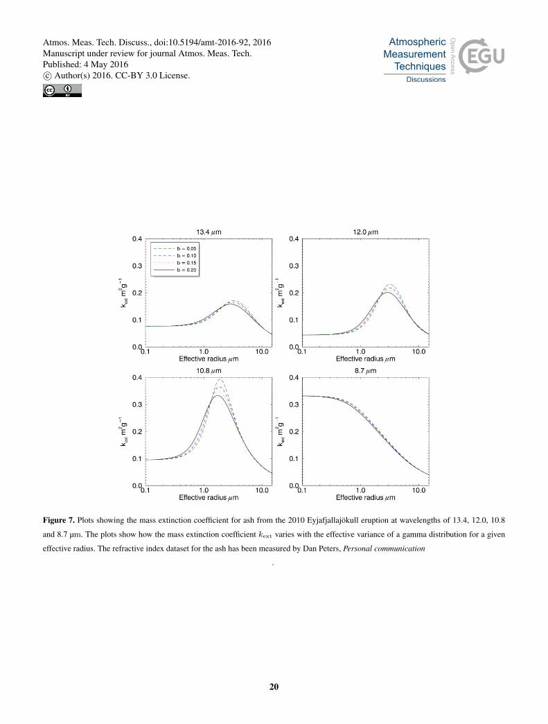
Figure 7. Plots showing the mass extinction coefficient for ash from the 2010 Eyjafjallajökull eruption at wavelengths of 13.4, 12.0, 10.8

and 8.7 µm. The plots show how the mass extinction coefficient kext varies with the effective variance of a gamma distribution for a given

effective radius. The refractive index dataset for the ash has been measured by Dan Peters, Personal communication

.

20


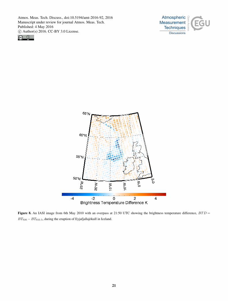
Figure 8. An IASI image from 6th May 2010 with an overpass at 21:50 UTC showing the brightness temperature difference, BTD =

BT926−BT833.5, during the eruption of Eyjafjallajökull in Iceland.

21


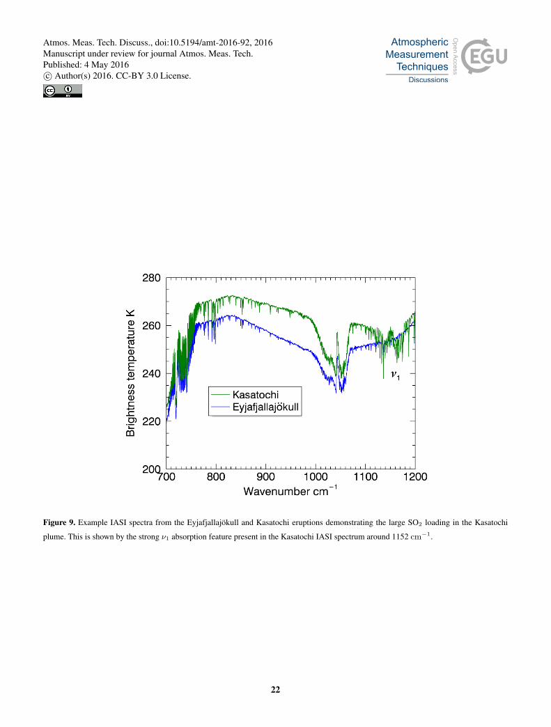
Figure 9. Example IASI spectra from the Eyjafjallajökull and Kasatochi eruptions demonstrating the large SO2 loading in the Kasatochi

plume. This is shown by the strong ν1 absorption feature present in the Kasatochi IASI spectrum around 1152 cm−1.

22


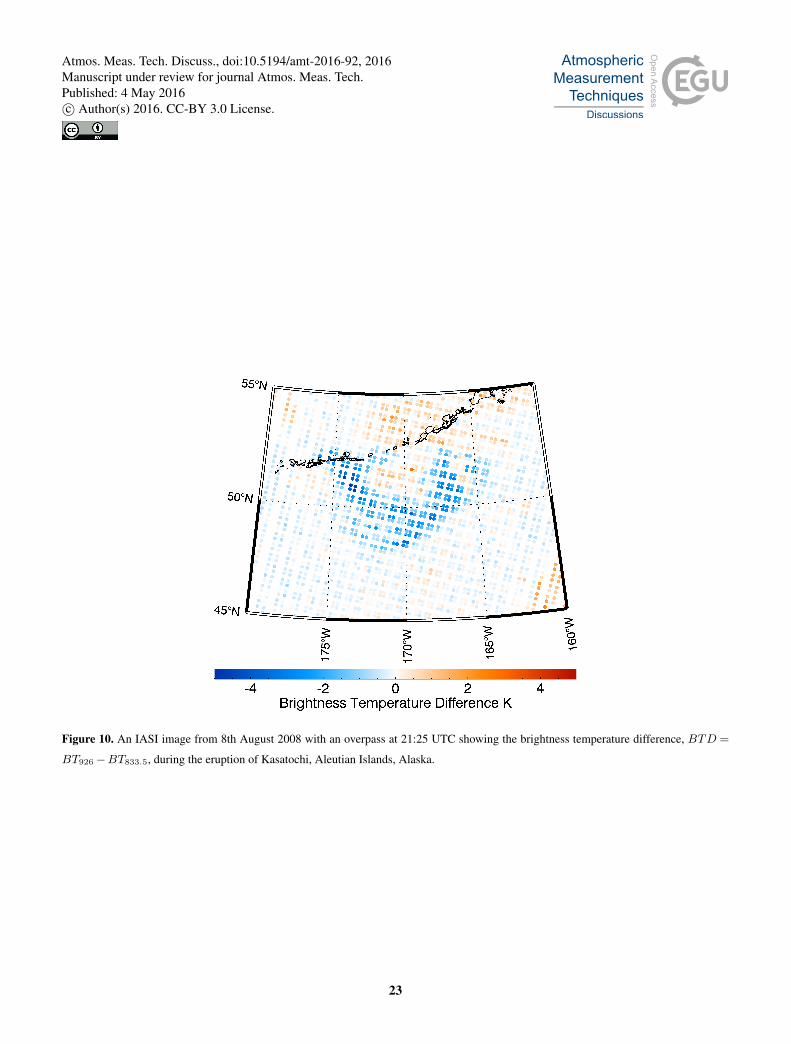
Figure 10. An IASI image from 8th August 2008 with an overpass at 21:25 UTC showing the brightness temperature difference, BTD =

BT926−BT833.5, during the eruption of Kasatochi, Aleutian Islands, Alaska.

23


Figure 11. The retrieval of (a) geometric standard deviation of a log-normal particle size distribution, (b) ash column loading, (c) effective

radius and (d) cloud top altitude from an IASI image from 6th May 2010 with an overpass at 21:50 UTC during the eruption of Eyjafjallajökull

in Iceland.

24


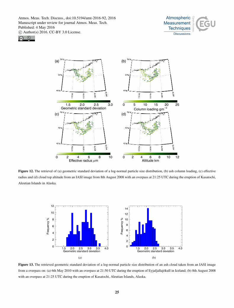
Figure 12. The retrieval of (a) geometric standard deviation of a log-normal particle size distribution, (b) ash column loading, (c) effective

radius and (d) cloud top altitude from an IASI image from 8th August 2008 with an overpass at 21:25 UTC during the eruption of Kasatochi,

Aleutian Islands in Alaska.

(a) (b)

Figure 13. The retrieved geometric standard deviation of a log-normal particle size distribution of an ash cloud taken from an IASI image

from a overpass on: (a) 6th May 2010 with an overpass at 21:50 UTC during the eruption of Eyjafjallajökull in Iceland; (b) 8th August 2008

with an overpass at 21:25 UTC during the eruption of Kasatochi, Aleutian Islands, Alaska.

25


inferring the size distribution of volcanic ash from iasi ... · inferring the size distribution of...

Documents