arX

iv:1

707.

0204

7v2

[cs

.DB

] 9

Oct

201

7

InferSpark: Statistical Inference at Scale

Zhuoyue Zhao 1, Jialing Pei 1, Eric Lo 2, Kenny Q. Zhu 1, Chris Liu 2

1Shanghai Jiao Tong University 2Hong Kong Polytechnic University

{zzy7896321@, peijialing@, kzhu@cs}.sjtu.edu.cn {ericlo, cscyliu}@comp.polyu.edu.hk

ABSTRACT

The Apache Spark stack has enabled fast large-scale dataprocessing. Despite a rich library of statistical models andinference algorithms, it does not give domain users the abil-ity to develop their own models. The emergence of proba-bilistic programming languages has showed the promise ofdeveloping sophisticated probabilistic models in a succinctand programmatic way. These frameworks have the poten-tial of automatically generating inference algorithms for theuser defined models and answering various statistical queriesabout the model. It is a perfect time to unite these twogreat directions to produce a programmable big data analy-sis framework. We thus propose, InferSpark, a probabilisticprogramming framework on top of Apache Spark. Efficientstatistical inference can be easily implemented on this frame-work and inference process can leverage the distributed mainmemory processing power of Spark. This framework makesstatistical inference on big data possible and speed up thepenetration of probabilistic programming into the data en-gineering domain.

1. INTRODUCTIONStatistical inference is an important technique to express

hypothesis and reason about data in data analytical tasks.Today, many big data applications are based on statisticalinference. Examples include topic modeling [5, 21], senti-ment analysis [22, 13, 16], spam filtering [19], to name afew.

One of most critical steps of statistical inference is to con-struct a statistical model to formally represent the under-lying statistical inference task [8]. The development of astatistical model is never trivial because a domain user mayhave to devise and implement many different models be-fore finding a promising one for a specific task. Currently,most scalable machine learning libraries (e.g. MLlib [4])only contain standard models like support vector machine,linear regression, latent Dirichlet allocation (LDA) [5], etc.To carry out statistical inference on customized models withbig data, the user has to implement her own models and in-ference codes on a distributed framework like Apache Spark[26] and Hadoop [1].

Developing inference code requires extensive knowledgein both statistical inference and programming techniques indistributed frameworks. Moreover, model definitions, infer-ence algorithms, and data processing tasks are all mixed upin the resulting code, making it hard to debug and reasonabout. For even a slight alteration to the model in questof the most promising one, the model designer will have to

re-derive the formulas and re-implement the inference codes,which is tedious and error-prone.

In this paper, we present InferSpark, a probabilistic pro-

gramming framework on top of Spark. Probabilistic pro-gramming is an emerging paradigm that allows statisticianand domain users to succinctly express a model definitionwithin a host programming language and transfers the bur-den of implementing the inference algorithm from the userto the compilers and runtime systems [3]. For example, In-fer.NET [17] is a probabilistic programming framework thatextends C#. The user can express, say, a Bayesian networkin C# and the compiler will generate code to perform infer-ence on it. Such code could be as efficient as the implemen-tation of the same inference algorithm carefully optimizedby an experienced programmer.

So far, the emphasis of probabilistic programming hasbeen put on the expressiveness of the languages and thedevelopment of efficient inference algorithms (e.g., varia-tional message passing [24], Gibbs sampling [6], Metropolis-Hastings sampling [7]) to handle a wider range of statisticalmodels. The issue of scaling out these frameworks, however,has not been addressed. For example, Infer.NET only workson a single machine. When we tried to use Infer.NET totrain an LDA model of 96 topics and 9040-word vocabularyon only 3% of Wikipedia articles, the actual memory require-ment has already exceeded 512GB, the maximum memoryof most commodity servers today. The goal of InferSparkis thus to bring probabilistic programming to Spark, a pre-dominant distributed data analytic platform, for carryingout statistical inference at scale. The InferSpark projectconsists of two parts:

(a) Extending Scala to support probabilistic program-ming

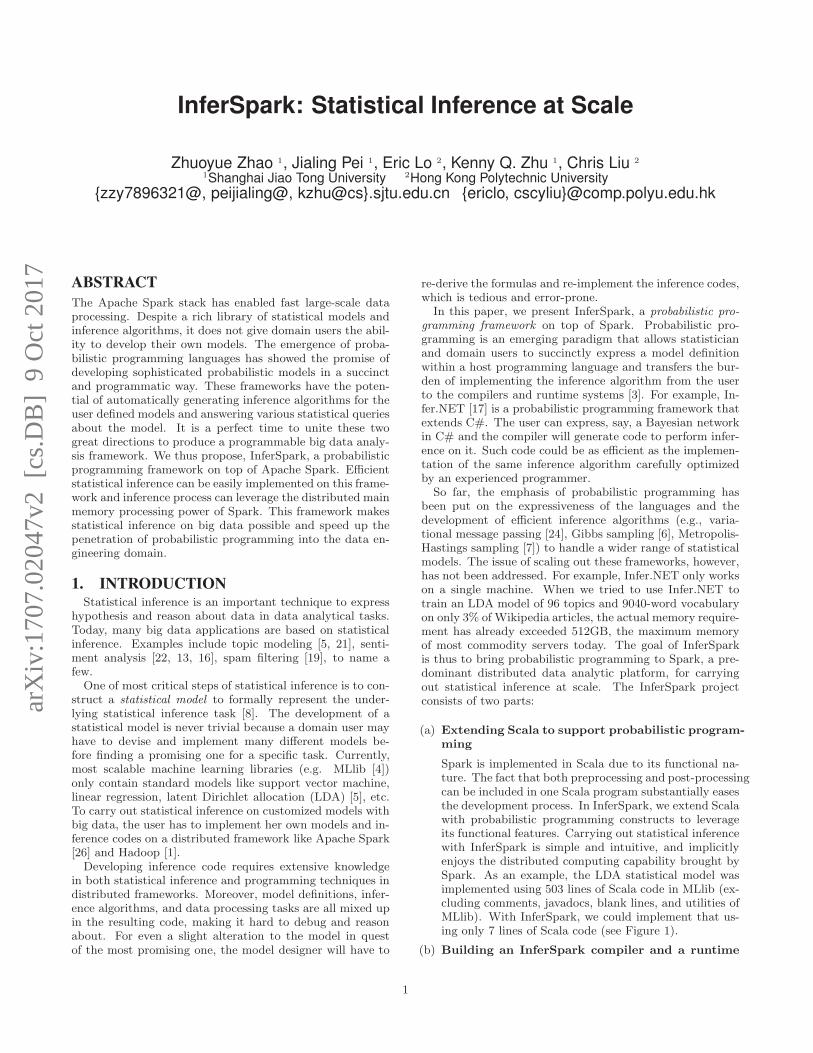
Spark is implemented in Scala due to its functional na-ture. The fact that both preprocessing and post-processingcan be included in one Scala program substantially easesthe development process. In InferSpark, we extend Scalawith probabilistic programming constructs to leverageits functional features. Carrying out statistical inferencewith InferSpark is simple and intuitive, and implicitlyenjoys the distributed computing capability brought bySpark. As an example, the LDA statistical model wasimplemented using 503 lines of Scala code in MLlib (ex-cluding comments, javadocs, blank lines, and utilities ofMLlib). With InferSpark, we could implement that us-ing only 7 lines of Scala code (see Figure 1).

(b) Building an InferSpark compiler and a runtime

1

1 @Model

2 class LDA(K: Long, V: Long, alpha: Double, beta: Double){

3 val phi = (0L until K).map{_ => Dirichlet(beta, K)}

4 val theta = ?.map{_ => Dirichlet(alpha, K)}

5 val z = theta.map{theta => ?.map{_ => Categorical(theta)

}}

6 val x = z.map{_.map{z => Categorical(phi(z))}}

7 }

Figure 1: Definition of Latent Dirichlet AllocationModel

system

InferSpark compiles InferSpark models into Scala classesand objects that implement the inference algorithms witha set of API. The user can call the API from their Scalaprograms to specify the input (observed) data and queryabout the model (e.g. compute the expectation of somerandom variables or retrieve the parameters of the pos-terior distributions).

Currently, InferSpark supports Bayesian network models.Bayesian network is a major branch of probabilistic graphi-cal model and it has already covered models like naive Bayes,LDA, TSM [16], etc. The goal of this paper is to describethe workflow, architecture, and Bayesian network implemen-tation of InferSpark. We will open-source InferSpark andsupport other models (e.g., Markov networks) afterwards.

To the best of our knowledge, InferSpark is the first en-deavor to bring probabilistic programming into the (big)data engineering domain. Efforts like MLI [20] and Sys-temML [10] all aim at easing the difficulty of developingdistributed machine learning techniques (e.g., stochastic gra-dient descent (SGD)). InferSpark aims at easing the com-plexity of developing custom statistical models, with statis-tician, data scientists, and machine learning researchers asthe target users. This paper presents the following technicalcontributions of InferSpark so far.

(a) We present the extension of Scala’s syntax that can ex-press various sophisticated Bayesian network models withease.

(b) We present the details of compiling and executing anInferSpark program on Spark. That includes the mech-anism of automatic generating efficient inference codesthat include checkpointing (to avoid long lineage), propertiming of caching and anti-caching (to improve efficiencyunder memory constraint), and partitioning (to avoidunnecessary replication and shuffling).

(c) We present an empirical study that shows InferSparkcan enable statistical inference on both customized andstandard models at scale.

The remainder of this paper is organized as follows: Sec-tion 2 presents the essential background for this paper. Sec-tion 3 then gives an overview of InferSpark. Section 4 givesthe implementation details of InferSpark. Section 5 presentsan evaluation study of the current version of InferSpark.Section 6 discusses related work and Section 7 contains ourconcluding remarks.

2. BACKGROUNDThis section presents some preliminary knowledge about

statistical inference and, in particular, Bayesian inference

using variational message passing, a popular variational in-ference algorithm, as well as its implementation concerns onApache Spark/GraphX stack.

2.1 Statistical InferenceStatistical inference is a common machine learning task

of obtaining the properties of the underlying distribution ofdata. For example, one can infer from many coin tosses theprobability of the coin turning up head by counting howmany tosses out of the all tosses are head. There are twodifferent approaches to model the number of heads: the fre-quentist approach and the Bayesian approach.

Let N be the total number of tosses and H be the numberof heads. In frequentist approach, the probability of cointurning up head is viewed as an unknown fixed parameterso the best guess φ would be the number of heads H in theresults over the total number of tosses N .

φ =H

N

In Bayesian approach, the probability of head is viewedas a hidden random variable drawn from a prior distribu-tion, e.g., Beta(1, 1), the uniform distribution over [0, 1].According to the Bayes Theorem, the posterior distributionof the probability of coin turning up head can be calculatedas follows:

p(φ|x) = φH(1− φ)N−Hf(φ; 1, 1)∫

1

0φH(1− φ)N−Hf(φ; 1, 1)dφ

= f(φ;H + 1, N −H + 1) (1)

where f(·;α, β) is the probability density function (PDF) ofBeta(α, β) and x is the outcome of N coin tosses.

The frequentist approach needs smoothing and regular-ization techniques to generalize on unseen data while theBayesian approach does not because the latter can capturethe uncertainty by modeling the parameters as random vari-ables.

2.2 Probabilistic Graphical ModelProbabilistic graphical model [14] (PGM) is a graphical

representation of the conditional dependencies in statisticalinference. Two types of PGM are widely used: Bayesiannetworks and Markov networks. Markov networks are undi-rected graphs while Bayesian networks are directed acyclicgraphs. Each type of PGM can represent certain indepen-dence constraints that the other cannot represent. InferSparkcurrently supports Bayesian networks and regards Markovnetworks as the next step.

N

�

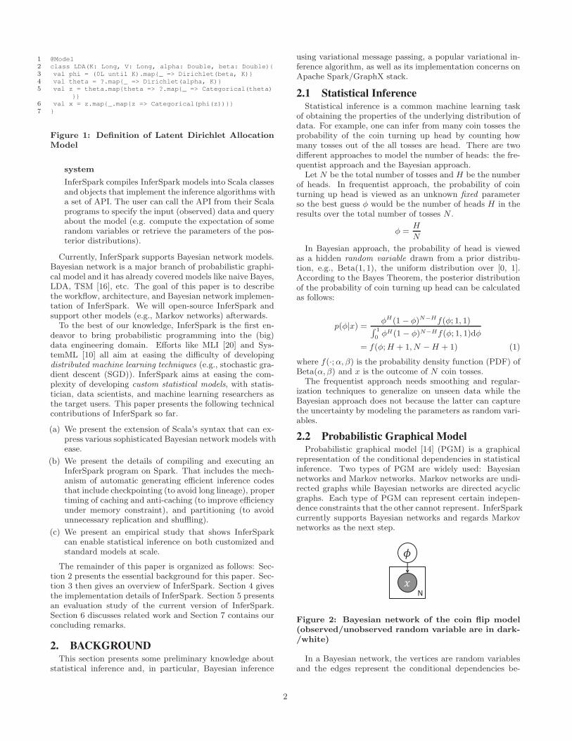
Figure 2: Bayesian network of the coin flip model(observed/unobserved random variable are in dark-/white)

In a Bayesian network, the vertices are random variablesand the edges represent the conditional dependencies be-

2

2

N

�

!

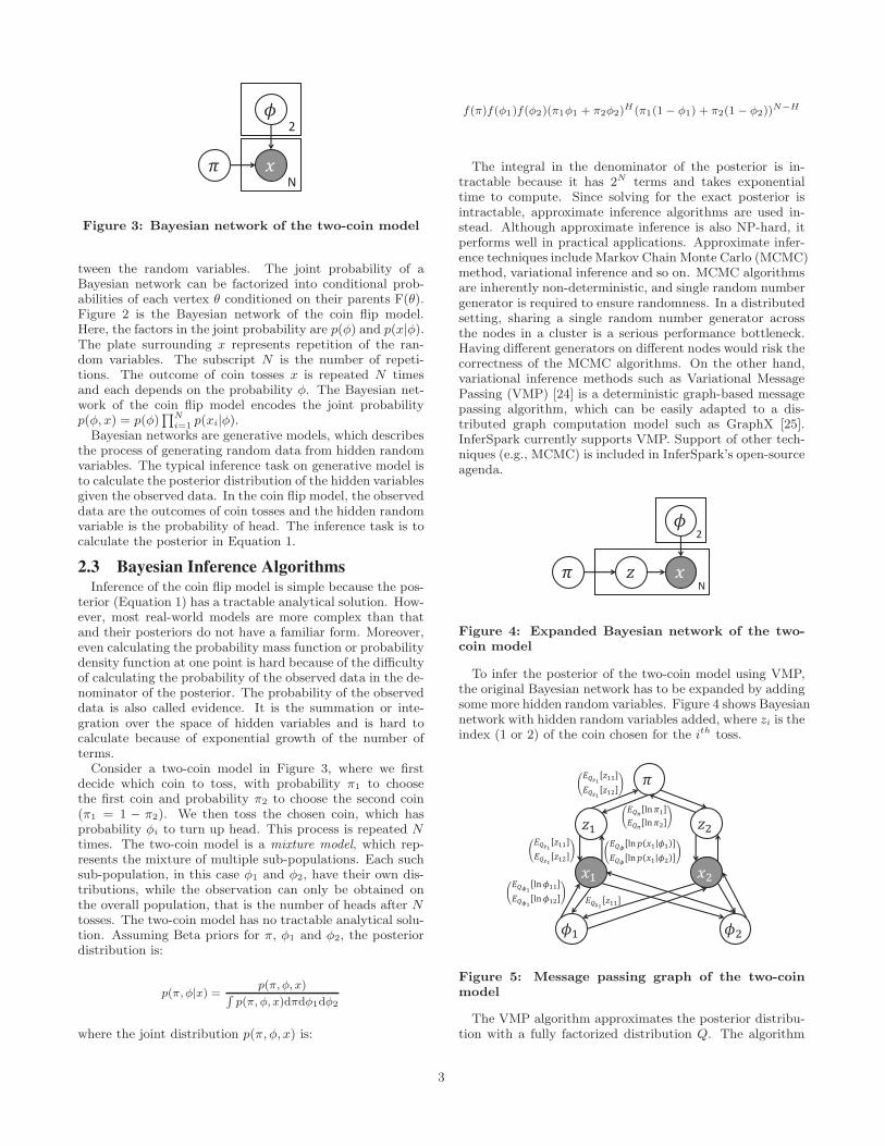
Figure 3: Bayesian network of the two-coin model

tween the random variables. The joint probability of aBayesian network can be factorized into conditional prob-abilities of each vertex θ conditioned on their parents F(θ).Figure 2 is the Bayesian network of the coin flip model.Here, the factors in the joint probability are p(φ) and p(x|φ).The plate surrounding x represents repetition of the ran-dom variables. The subscript N is the number of repeti-tions. The outcome of coin tosses x is repeated N timesand each depends on the probability φ. The Bayesian net-work of the coin flip model encodes the joint probabilityp(φ, x) = p(φ)

∏N

i=1p(xi|φ).

Bayesian networks are generative models, which describesthe process of generating random data from hidden randomvariables. The typical inference task on generative model isto calculate the posterior distribution of the hidden variablesgiven the observed data. In the coin flip model, the observeddata are the outcomes of coin tosses and the hidden randomvariable is the probability of head. The inference task is tocalculate the posterior in Equation 1.

2.3 Bayesian Inference AlgorithmsInference of the coin flip model is simple because the pos-

terior (Equation 1) has a tractable analytical solution. How-ever, most real-world models are more complex than thatand their posteriors do not have a familiar form. Moreover,even calculating the probability mass function or probabilitydensity function at one point is hard because of the difficultyof calculating the probability of the observed data in the de-nominator of the posterior. The probability of the observeddata is also called evidence. It is the summation or inte-gration over the space of hidden variables and is hard tocalculate because of exponential growth of the number ofterms.

Consider a two-coin model in Figure 3, where we firstdecide which coin to toss, with probability π1 to choosethe first coin and probability π2 to choose the second coin(π1 = 1 − π2). We then toss the chosen coin, which hasprobability φi to turn up head. This process is repeated N

times. The two-coin model is a mixture model, which rep-resents the mixture of multiple sub-populations. Each suchsub-population, in this case φ1 and φ2, have their own dis-tributions, while the observation can only be obtained onthe overall population, that is the number of heads after Ntosses. The two-coin model has no tractable analytical solu-tion. Assuming Beta priors for π, φ1 and φ2, the posteriordistribution is:

p(π, φ|x) =p(π, φ, x)

∫p(π, φ, x)dπdφ1dφ2

where the joint distribution p(π, φ, x) is:

f(π)f(φ1)f(φ2)(π1φ1 + π2φ2)H (π1(1− φ1) + π2(1 − φ2))

N−H

The integral in the denominator of the posterior is in-tractable because it has 2N terms and takes exponentialtime to compute. Since solving for the exact posterior isintractable, approximate inference algorithms are used in-stead. Although approximate inference is also NP-hard, itperforms well in practical applications. Approximate infer-ence techniques include Markov Chain Monte Carlo (MCMC)method, variational inference and so on. MCMC algorithmsare inherently non-deterministic, and single random numbergenerator is required to ensure randomness. In a distributedsetting, sharing a single random number generator acrossthe nodes in a cluster is a serious performance bottleneck.Having different generators on different nodes would risk thecorrectness of the MCMC algorithms. On the other hand,variational inference methods such as Variational MessagePassing (VMP) [24] is a deterministic graph-based messagepassing algorithm, which can be easily adapted to a dis-tributed graph computation model such as GraphX [25].InferSpark currently supports VMP. Support of other tech-niques (e.g., MCMC) is included in InferSpark’s open-sourceagenda.

2

N

�

! "

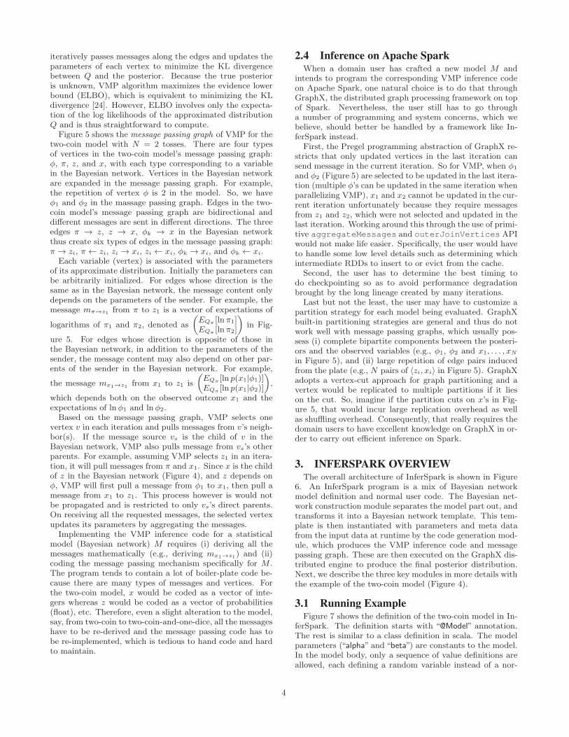
Figure 4: Expanded Bayesian network of the two-coin model

To infer the posterior of the two-coin model using VMP,the original Bayesian network has to be expanded by addingsome more hidden random variables. Figure 4 shows Bayesiannetwork with hidden random variables added, where zi is theindex (1 or 2) of the coin chosen for the ith toss.

��

�

!

"�#$%&

"��

#$%&"�'

#$( ln ) �� �

#$( ln ) �� '

#$* ln !�

#$* ln !' "'

�'

'

#$%&"��

#$%&"�'

#$+&"��

#$(&ln ��

#$(&ln �'

Figure 5: Message passing graph of the two-coinmodel

The VMP algorithm approximates the posterior distribu-tion with a fully factorized distribution Q. The algorithm

3

iteratively passes messages along the edges and updates theparameters of each vertex to minimize the KL divergencebetween Q and the posterior. Because the true posterioris unknown, VMP algorithm maximizes the evidence lowerbound (ELBO), which is equivalent to minimizing the KLdivergence [24]. However, ELBO involves only the expecta-tion of the log likelihoods of the approximated distributionQ and is thus straightforward to compute.

Figure 5 shows the message passing graph of VMP for thetwo-coin model with N = 2 tosses. There are four typesof vertices in the two-coin model’s message passing graph:φ, π, z, and x, with each type corresponding to a variablein the Bayesian network. Vertices in the Bayesian networkare expanded in the message passing graph. For example,the repetition of vertex φ is 2 in the model. So, we haveφ1 and φ2 in the massage passing graph. Edges in the two-coin model’s message passing graph are bidirectional anddifferent messages are sent in different directions. The threeedges π → z, z → x, φk → x in the Bayesian networkthus create six types of edges in the message passing graph:π → zi, π ← zi, zi → xi, zi ← xi, φk → xi, and φk ← xi.

Each variable (vertex) is associated with the parametersof its approximate distribution. Initially the parameters canbe arbitrarily initialized. For edges whose direction is thesame as in the Bayesian network, the message content onlydepends on the parameters of the sender. For example, themessage mπ→z1 from π to z1 is a vector of expectations of

logarithms of π1 and π2, denoted as

(

EQπ[ln π1]

EQπ[ln π2]

)

in Fig-

ure 5. For edges whose direction is opposite of those inthe Bayesian network, in addition to the parameters of thesender, the message content may also depend on other par-ents of the sender in the Bayesian network. For example,

the message mx1→z1 from x1 to z1 is

(

EQπ[ln p(x1|φ1)]

EQπ[ln p(x1|φ2)]

)

,

which depends both on the observed outcome x1 and theexpectations of lnφ1 and lnφ2.

Based on the message passing graph, VMP selects onevertex v in each iteration and pulls messages from v’s neigh-bor(s). If the message source vs is the child of v in theBayesian network, VMP also pulls message from vs’s otherparents. For example, assuming VMP selects z1 in an itera-tion, it will pull messages from π and x1. Since x is the childof z in the Bayesian network (Figure 4), and z depends onφ, VMP will first pull a message from φ1 to x1, then pull amessage from x1 to z1. This process however is would notbe propagated and is restricted to only vs’s direct parents.On receiving all the requested messages, the selected vertexupdates its parameters by aggregating the messages.

Implementing the VMP inference code for a statisticalmodel (Bayesian network) M requires (i) deriving all themessages mathematically (e.g., deriving mx1→z1) and (ii)coding the message passing mechanism specifically for M .The program tends to contain a lot of boiler-plate code be-cause there are many types of messages and vertices. Forthe two-coin model, x would be coded as a vector of inte-gers whereas z would be coded as a vector of probabilities(float), etc. Therefore, even a slight alteration to the model,say, from two-coin to two-coin-and-one-dice, all the messageshave to be re-derived and the message passing code has tobe re-implemented, which is tedious to hand code and hardto maintain.

2.4 Inference on Apache SparkWhen a domain user has crafted a new model M and

intends to program the corresponding VMP inference codeon Apache Spark, one natural choice is to do that throughGraphX, the distributed graph processing framework on topof Spark. Nevertheless, the user still has to go througha number of programming and system concerns, which webelieve, should better be handled by a framework like In-ferSpark instead.

First, the Pregel programming abstraction of GraphX re-stricts that only updated vertices in the last iteration cansend message in the current iteration. So for VMP, when φ1

and φ2 (Figure 5) are selected to be updated in the last itera-tion (multiple φ’s can be updated in the same iteration whenparallelizing VMP), x1 and x2 cannot be updated in the cur-rent iteration unfortunately because they require messagesfrom z1 and z2, which were not selected and updated in thelast iteration. Working around this through the use of primi-tive aggregateMessages and outerJoinVertices APIwould not make life easier. Specifically, the user would haveto handle some low level details such as determining whichintermediate RDDs to insert to or evict from the cache.

Second, the user has to determine the best timing todo checkpointing so as to avoid performance degradationbrought by the long lineage created by many iterations.

Last but not the least, the user may have to customize apartition strategy for each model being evaluated. GraphXbuilt-in partitioning strategies are general and thus do notwork well with message passing graphs, which usually pos-sess (i) complete bipartite components between the posteri-ors and the observed variables (e.g., φ1, φ2 and x1, . . . , xN

in Figure 5), and (ii) large repetition of edge pairs inducedfrom the plate (e.g., N pairs of 〈zi, xi〉 in Figure 5). GraphXadopts a vertex-cut approach for graph partitioning and avertex would be replicated to multiple partitions if it lieson the cut. So, imagine if the partition cuts on x’s in Fig-ure 5, that would incur large replication overhead as wellas shuffling overhead. Consequently, that really requires thedomain users to have excellent knowledge on GraphX in or-der to carry out efficient inference on Spark.

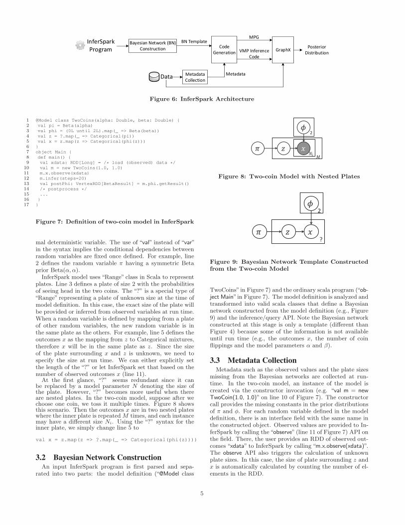
3. INFERSPARK OVERVIEWThe overall architecture of InferSpark is shown in Figure

6. An InferSpark program is a mix of Bayesian networkmodel definition and normal user code. The Bayesian net-work construction module separates the model part out, andtransforms it into a Bayesian network template. This tem-plate is then instantiated with parameters and meta datafrom the input data at runtime by the code generation mod-ule, which produces the VMP inference code and messagepassing graph. These are then executed on the GraphX dis-tributed engine to produce the final posterior distribution.Next, we describe the three key modules in more details withthe example of the two-coin model (Figure 4).

3.1 Running ExampleFigure 7 shows the definition of the two-coin model in In-

ferSpark. The definition starts with “@Model” annotation.The rest is similar to a class definition in scala. The modelparameters (“alpha” and “beta”) are constants to the model.In the model body, only a sequence of value definitions areallowed, each defining a random variable instead of a nor-

4

Bayesian Network (BN)

Construction

Data

InferSpark

Program

Metadata

Collection

BN Template

Metadata

Code

Generation

MPG

VMP Inference

Code

GraphXPosterior

Distribution

Figure 6: InferSpark Architecture

1 @Model class TwoCoins(alpha: Double, beta: Double) {

2 val pi = Beta(alpha)

3 val phi = (0L until 2L).map(_ => Beta(beta))

4 val z = ?.map(_ => Categorical(pi))

5 val x = z.map(z => Categorical(phi(z)))

6 }

7 object Main {

8 def main() {

9 val xdata: RDD[Long] = /* load (observed) data */

10 val m = new TwoCoins(1.0, 1.0)

11 m.x.observe(xdata)

12 m.infer(steps=20)

13 val postPhi: VertexRDD[BetaResult] = m.phi.getResult()

14 /* postprocess */

15 ...

16 }

17 }

Figure 7: Definition of two-coin model in InferSpark

mal deterministic variable. The use of “val” instead of “var”in the syntax implies the conditional dependencies betweenrandom variables are fixed once defined. For example, line2 defines the random variable π having a symmetric Betaprior Beta(α, α).

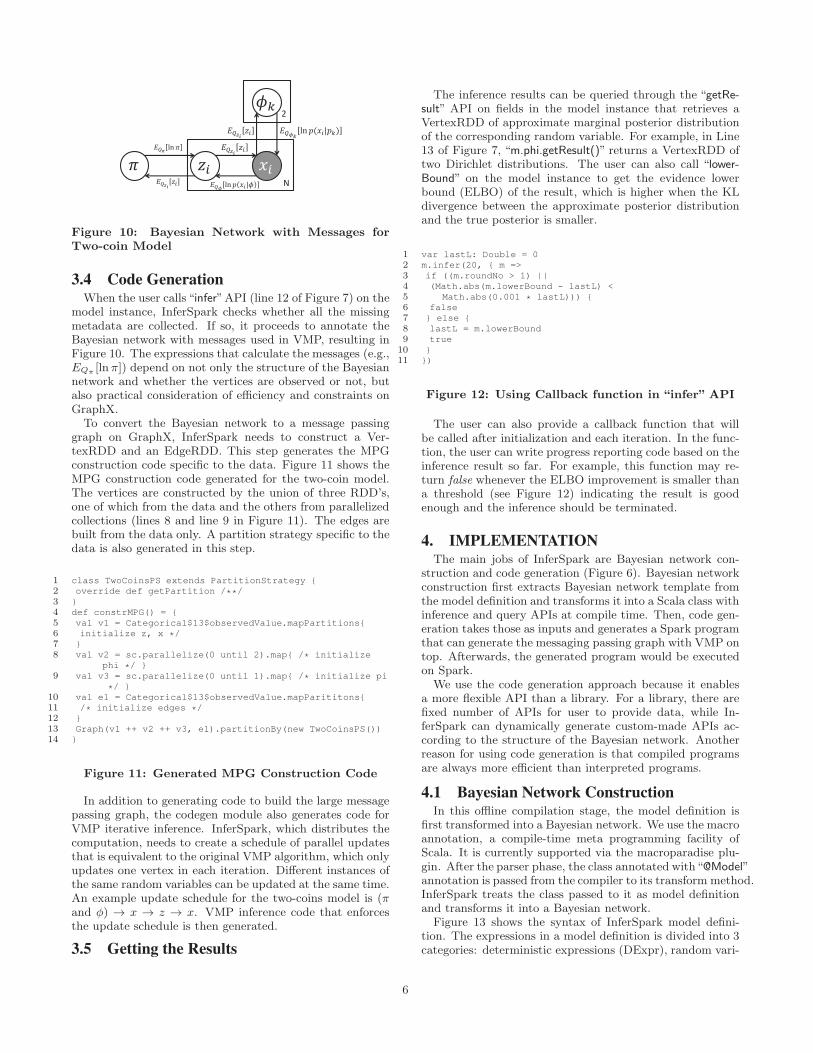
InferSpark model uses “Range” class in Scala to representplates. Line 3 defines a plate of size 2 with the probabilitiesof seeing head in the two coins. The “?” is a special type of“Range” representing a plate of unknown size at the time ofmodel definition. In this case, the exact size of the plate willbe provided or inferred from observed variables at run time.When a random variable is defined by mapping from a plateof other random variables, the new random variable is inthe same plate as the others. For example, line 5 defines theoutcomes x as the mapping from z to Categorical mixtures,therefore x will be in the same plate as z. Since the sizeof the plate surrounding x and z is unknown, we need tospecify the size at run time. We can either explicitly setthe length of the “?” or let InferSpark set that based on thenumber of observed outcomes x (line 11).

At the first glance, “?” seems redundant since it canbe replaced by a model parameter N denoting the size ofthe plate. However, “?” becomes more useful when thereare nested plates. In the two-coin model, suppose after wechoose one coin, we toss it multiple times. Figure 8 showsthis scenario. Then the outcomes x are in two nested plateswhere the inner plate is repeated M times, and each instancemay have a different size Ni. Using the “?” syntax for theinner plate, we simply change line 5 to

val x = z.map(z => ?.map(_ => Categorical(phi(z))))

3.2 Bayesian Network ConstructionAn input InferSpark program is first parsed and sepa-

rated into two parts: the model definition (“@Model class

2

� !

"

#

$ %

Figure 8: Two-coin Model with Nested Plates

2

?

�

! "

Figure 9: Bayesian Network Template Constructedfrom the Two-coin Model

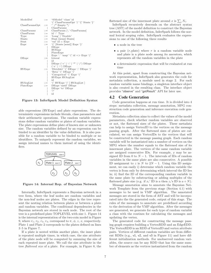
TwoCoins” in Figure 7) and the ordinary scala program (“ob-ject Main”in Figure 7). The model definition is analyzed andtransformed into valid scala classes that define a Bayesiannetwork constructed from the model definition (e.g., Figure9) and the inference/query API. Note the Bayesian networkconstructed at this stage is only a template (different thanFigure 4) because some of the information is not availableuntil run time (e.g., the outcomes x, the number of coinflippings and the model parameters α and β).

3.3 Metadata CollectionMetadata such as the observed values and the plate sizes

missing from the Bayesian networks are collected at run-time. In the two-coin model, an instance of the model iscreated via the constructor invocation (e.g. “val m = newTwoCoin(1.0, 1.0)” on line 10 of Figure 7). The constructorcall provides the missing constants in the prior distributionsof π and φ. For each random variable defined in the modeldefinition, there is an interface field with the same name inthe constructed object. Observed values are provided to In-ferSpark by calling the“observe” (line 11 of Figure 7) API onthe field. There, the user provides an RDD of observed out-comes “xdata” to InferSpark by calling “m.x.observe(xdata)”.The observe API also triggers the calculation of unknownplate sizes. In this case, the size of plate surrounding z andx is automatically calculated by counting the number of el-ements in the RDD.

5

N

2

��

!

" #�

$%&'ln ((��|(!)

$%+ ln "

$%,-#� $%& ln ( ��|

$%,-#�

$%,-#�

Figure 10: Bayesian Network with Messages forTwo-coin Model

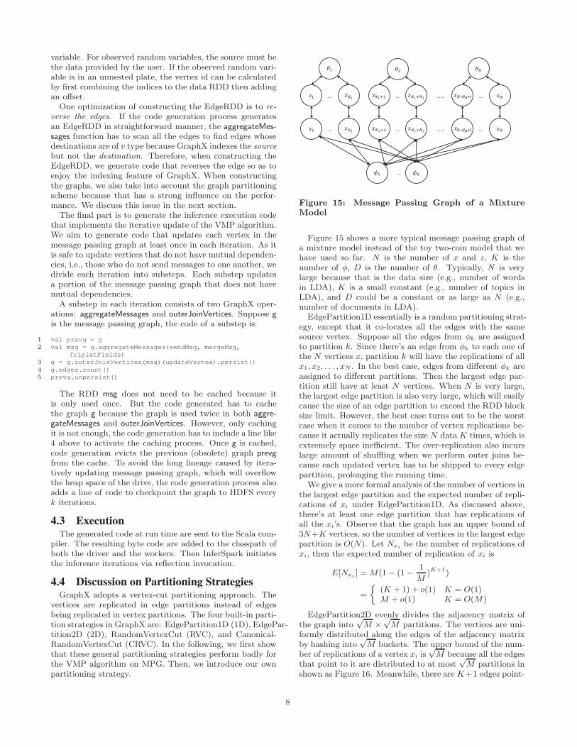
3.4 Code GenerationWhen the user calls “infer”API (line 12 of Figure 7) on the

model instance, InferSpark checks whether all the missingmetadata are collected. If so, it proceeds to annotate theBayesian network with messages used in VMP, resulting inFigure 10. The expressions that calculate the messages (e.g.,EQπ

[ln π]) depend on not only the structure of the Bayesiannetwork and whether the vertices are observed or not, butalso practical consideration of efficiency and constraints onGraphX.

To convert the Bayesian network to a message passinggraph on GraphX, InferSpark needs to construct a Ver-texRDD and an EdgeRDD. This step generates the MPGconstruction code specific to the data. Figure 11 shows theMPG construction code generated for the two-coin model.The vertices are constructed by the union of three RDD’s,one of which from the data and the others from parallelizedcollections (lines 8 and line 9 in Figure 11). The edges arebuilt from the data only. A partition strategy specific to thedata is also generated in this step.

1 class TwoCoinsPS extends PartitionStrategy {

2 override def getPartition /**/

3 }

4 def constrMPG() = {

5 val v1 = Categorical$13$observedValue.mapPartitions{

6 initialize z, x */

7 }

8 val v2 = sc.parallelize(0 until 2).map{ /* initialize

phi */ }

9 val v3 = sc.parallelize(0 until 1).map{ /* initialize pi

*/ }

10 val e1 = Categorical$13$observedValue.mapParititons{

11 /* initialize edges */

12 }

13 Graph(v1 ++ v2 ++ v3, e1).partitionBy(new TwoCoinsPS())

14 }

Figure 11: Generated MPG Construction Code

In addition to generating code to build the large messagepassing graph, the codegen module also generates code forVMP iterative inference. InferSpark, which distributes thecomputation, needs to create a schedule of parallel updatesthat is equivalent to the original VMP algorithm, which onlyupdates one vertex in each iteration. Different instances ofthe same random variables can be updated at the same time.An example update schedule for the two-coins model is (πand φ) → x → z → x. VMP inference code that enforcesthe update schedule is then generated.

3.5 Getting the Results

The inference results can be queried through the “getRe-sult” API on fields in the model instance that retrieves aVertexRDD of approximate marginal posterior distributionof the corresponding random variable. For example, in Line13 of Figure 7, “m.phi.getResult()” returns a VertexRDD oftwo Dirichlet distributions. The user can also call “lower-Bound” on the model instance to get the evidence lowerbound (ELBO) of the result, which is higher when the KLdivergence between the approximate posterior distributionand the true posterior is smaller.

1 var lastL: Double = 0

2 m.infer(20, { m =>

3 if ((m.roundNo > 1) ||

4 (Math.abs(m.lowerBound - lastL) <

5 Math.abs(0.001 * lastL))) {

6 false

7 } else {

8 lastL = m.lowerBound

9 true

10 }

11 })

Figure 12: Using Callback function in “infer” API

The user can also provide a callback function that willbe called after initialization and each iteration. In the func-tion, the user can write progress reporting code based on theinference result so far. For example, this function may re-turn false whenever the ELBO improvement is smaller thana threshold (see Figure 12) indicating the result is goodenough and the inference should be terminated.

4. IMPLEMENTATIONThe main jobs of InferSpark are Bayesian network con-

struction and code generation (Figure 6). Bayesian networkconstruction first extracts Bayesian network template fromthe model definition and transforms it into a Scala class withinference and query APIs at compile time. Then, code gen-eration takes those as inputs and generates a Spark programthat can generate the messaging passing graph with VMP ontop. Afterwards, the generated program would be executedon Spark.

We use the code generation approach because it enablesa more flexible API than a library. For a library, there arefixed number of APIs for user to provide data, while In-ferSpark can dynamically generate custom-made APIs ac-cording to the structure of the Bayesian network. Anotherreason for using code generation is that compiled programsare always more efficient than interpreted programs.

4.1 Bayesian Network ConstructionIn this offline compilation stage, the model definition is

first transformed into a Bayesian network. We use the macroannotation, a compile-time meta programming facility ofScala. It is currently supported via the macroparadise plu-gin. After the parser phase, the class annotated with“@Model”annotation is passed from the compiler to its transform method.InferSpark treats the class passed to it as model definitionand transforms it into a Bayesian network.

Figure 13 shows the syntax of InferSpark model defini-tion. The expressions in a model definition is divided into 3categories: deterministic expressions (DExpr), random vari-

6

ModelDef ::= ‘@Model’ ‘class’ id‘(’ ClassParamsOpt ‘)’ ‘{’ Stmts ‘}’

ClassParamsOpt ::= ‘’ /* Empty */| ClassParams

ClassParams ::= ClassParam [‘,’ ClassParams]ClassParam ::= id ‘:’ TypeType ::= ‘Long’ | ‘Double’Stmts ::= Stmt [[semi] Stmts]Stmt ::= ‘val’ id = ExprExpr ::= ‘{’ [Stmts [semi]] Expr ‘}’

| DExpr| RVExpr| PlateExpr| Expr ‘.’ ‘map’ ‘(’ id => Expr ‘)’

DExpr ::= Literal| id| DExpr (‘+’ | ‘-’ | ‘*’ | ‘/’) DExpr| (‘+’ | ‘-’) DExpr

RVExpr ::= ‘Dirichlet’ ‘(’ DExpr ‘,’ DExpr ‘)’| ‘Beta’ ‘(’ DExpr ‘)’| ‘Categorical’ ‘(’ Expr ‘)’| RVExpr RVArgList| id

RVArgList ::= ‘(’ RVExpr ‘)’ [ RVArgList ]PlateExpr ::= DExpr ‘until’ DExpr

| DExpr ‘to’ DExpr| ‘?’| id

Figure 13: InferSpark Model Definition Syntax

able expressions (RVExpr) and plate expressions. The de-terministic expressions include literals, class parameters andtheir arithemetic operations. The random variable expres-sions define random variables or plates of random variables.The plate expressions define plate of known size or unknownsize. The random variables defined by an expression can bebinded to an identifier by the value definition. It is also pos-sible for a random variable to be binded to multiple or noidentifiers. To uniquely represent the random variables, weassign internal names to them instead of using the identi-fiers.

TOPLEVEL size=1

Plate 1 size=2��

� �!

Plate 2 size=?

�"

Figure 14: Internal Rep. of Bayesian Network

Internally, InferSpark represents a Bayesian network in atree form, where the leaf nodes are random variables andthe non-leaf nodes are plates. The edges in the tree repre-sent the nesting relation between plates or between a plateand random variables. The conditional dependencies in theBayesian network are stored in each node. The root of thetree is a predefined plate TOPLEVEL with size 1. Figure 14is the internal representation of the two-coin model in Figure9, where r1, r2, r3, r4, correspond to π, φ, z, x, respectively.Plate 1 and Plate 2 correponds to the plates defined on lines3–5 in Figure 7.

If a plate is nested within another plate, the inner plateis repeated multiple times, in which case, the size attributeof the plate node will be computed by summing the size ofeach repeated inner plate. We call the size attribute in thetree flattened size of a plate. For example, in Figure 8, the

flattened size of the innermost plate around x is∑

iNi.

InferSpark recursively descends on the abstract syntaxtree (AST) of the model definition to construct the Bayesiannetwork. In the model definition, InferSpark follows the nor-mal lexical scoping rules. InferSpark evaluates the expres-sions to one of the following three results

• a node in the tree

• a pair (r,plate) where r is a random variable nodeand plate is a plate node among its ancestors, whichrepresents all the random variables in the plate

• a determinstic expression that will be evaluated at runtime

At this point, apart from constructing the Bayesian net-work representation, InferSpark also generates the code formetadata collection, a module used in stage 2. For eachrandom variable name bindings, a singleton interface objectis also created in the resulting class. The interface objectprovides “observe” and “getResult” API for later use.

4.2 Code GenerationCode generation happens at run time. It is divided into 4

steps: metadata collection, message annotation, MPG con-struction code generation and inference execution code gen-eration.

Metadata collection aims to collect the values of the modelparameters, check whether random variables are observedor not, the flattened sizes of the plates. These metadatacan help to assign VertexID to the vertices on the messagepassing graph. After the flattened sizes of plates are cal-culated, we can assign VertexIDs to the vertices that willbe constructed in the message passing graph. Each randomvariable will be instantiated into a number of vertices on theMPG where the number equals to the flattened size of itsinnermost plate. The vertices of the same random variableare assigned consecutive IDs. For example, x may be as-signed ID from 0 to N − 1. The intervals of IDs of randomvariables in the same plate are also consecutive. A possibleID assignment to z is N to 2N − 1. Using this ID assign-ment, we can easily i) determine which random variable thevertex is from only by determining which interval the ID liesin; ii) find the ID of the corresponding random variable inthe same plate by substracting or adding multiples of theflattened plate size (e.g. if xi’ ID is a then zi’s ID is a+N).

Message annotation aims to annotate the Bayesian Net-work Template from the previous stage (Section 4.1) withmessages to be used in VMP algorithm. The annotatedmessages are stored in the form of AST and will be incorpo-rated into the the generated code, output of this stage. Therules of the messages to annotate are predefined accordingto the derivation of the VMP algorithm. After the messagesare generated, we generate for each type of random variablea class with the routines for calculating the messages andupdating the vertex.

The generated code for constructing the message pass-ing graph requires building a VertexRDD and an EdgeEDD.The VertexRDD is an RDD of VertexID and vertex attributepairs. Vertices of different random variables are from differ-ent RDDs (e.g., v1, v2, and v3 in Figure 11) and have dif-ferent initialization methods. For unobserved random vari-ables, the source can be any RDD that has the same num-ber of elements as the vertices instantiated from the random

7

variable. For observed random variables, the source must bethe data provided by the user. If the observed random vari-able is in an unnested plate, the vertex id can be calculatedby first combining the indices to the data RDD then addingan offset.

One optimization of constructing the EdgeRDD is to re-

verse the edges. If the code generation process generatesan EdgeRDD in straightforward manner, the aggregateMes-sages function has to scan all the edges to find edges whosedestinations are of v type because GraphX indexes the sourcebut not the destination. Therefore, when constructing theEdgeRDD, we generate code that reverses the edge so as toenjoy the indexing feature of GraphX. When constructingthe graphs, we also take into account the graph partitioningscheme because that has a strong influence on the perfor-mance. We discuss this issue in the next section.

The final part is to generate the inference execution codethat implements the iterative update of the VMP algorithm.We aim to generate code that updates each vertex in themessage passing graph at least once in each iteration. As itis safe to update vertices that do not have mutual dependen-cies, i.e., those who do not send messages to one another, wedivide each iteration into substeps. Each substep updatesa portion of the message passing graph that does not havemutual dependencies.

A substep in each iteration consists of two GraphX oper-ations: aggregateMessages and outerJoinVertices. Suppose gis the message passing graph, the code of a substep is:

1 val prevg = g

2 val msg = g.aggregateMessages(sendMsg, mergeMsg,

TripletFields)

3 g = g.outerJoinVertices(msg)(updateVertex).persist()

4 g.edges.count()

5 prevg.unpersist()

The RDD msg does not need to be cached because itis only used once. But the code generated has to cachethe graph g because the graph is used twice in both aggre-gateMessages and outerJoinVertices. However, only cachingit is not enough, the code generation has to include a line like4 above to activate the caching process. Once g is cached,code generation evicts the previous (obsolete) graph prevgfrom the cache. To avoid the long lineage caused by itera-tively updating message passing graph, which will overflowthe heap space of the drive, the code generation process alsoadds a line of code to checkpoint the graph to HDFS everyk iterations.

4.3 ExecutionThe generated code at run time are sent to the Scala com-

piler. The resulting byte code are added to the classpath ofboth the driver and the workers. Then InferSpark initiatesthe inference iterations via reflection invocation.

4.4 Discussion on Partitioning StrategiesGraphX adopts a vertex-cut partitioning approach. The

vertices are replicated in edge partitions instead of edgesbeing replicated in vertex partitions. The four built-in parti-tion strategies in GraphX are: EdgePartition1D (1D), EdgePar-tition2D (2D), RandomVertexCut (RVC), and Canonical-RandomVertexCut (CRVC). In the following, we first showthat these general partitioning strategies perform badly forthe VMP algorithm on MPG. Then, we introduce our ownpartitioning strategy.

� �!"… �!"# �!"#!$… �!%!&# �!………

' '!"… '!"# '!"#!$… �!%!&# �!………

( ()…

* *+ *,

Figure 15: Message Passing Graph of a MixtureModel

Figure 15 shows a more typical message passing graph ofa mixture model instead of the toy two-coin model that wehave used so far. N is the number of x and z, K is thenumber of φ, D is the number of θ. Typically, N is verylarge because that is the data size (e.g., number of wordsin LDA), K is a small constant (e.g., number of topics inLDA), and D could be a constant or as large as N (e.g.,number of documents in LDA).

EdgePartition1D essentially is a random partitioning strat-egy, except that it co-locates all the edges with the samesource vertex. Suppose all the edges from φk are assignedto partition k. Since there’s an edge from φk to each one ofthe N vertices x, partition k will have the replications of allx1, x2, . . . , xN . In the best case, edges from different φk areassigned to different partitions. Then the largest edge par-tition still have at least N vertices. When N is very large,the largest edge partition is also very large, which will easilycause the size of an edge partition to exceed the RDD blocksize limit. However, the best case turns out to be the worstcase when it comes to the number of vertex replications be-cause it actually replicates the size N data K times, which isextremely space inefficient. The over-replication also incurslarge amount of shuffling when we perform outer joins be-cause each updated vertex has to be shipped to every edgepartition, prolonging the running time.

We give a more formal analysis of the number of vertices inthe largest edge partition and the expected number of repli-cations of xi under EdgePartition1D. As discussed above,there’s at least one edge partition that has replications ofall the xi’s. Observe that the graph has an upper bound of3N+K vertices, so the number of vertices in the largest edgepartition is O(N). Let Nxi

be the number of replications ofxi, then the expected number of replication of xi is

E[Nxi] = M(1− (1− 1

M)K+1)

=

{

(K + 1) + o(1) K = O(1)M + o(1) K = O(M)

EdgePartition2D evenly divides the adjacency matrix ofthe graph into

√M ×

√M partitions. The vertices are uni-

formly distributed along the edges of the adjacency matrixby hashing into

√M buckets. The upper bound of the num-

ber of replications of a vertex xi is√M because all the edges

that point to it are distributed to at most√M partitions in

shown as Figure 16. Meanwhile, there are K+1 edges point-

8

Dst

Src

��

��

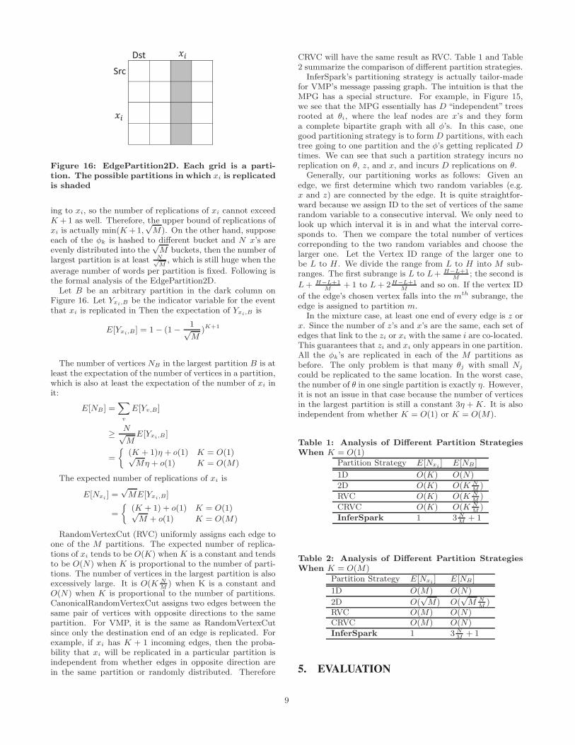
Figure 16: EdgePartition2D. Each grid is a parti-tion. The possible partitions in which xi is replicatedis shaded

ing to xi, so the number of replications of xi cannot exceedK +1 as well. Therefore, the upper bound of replications ofxi is actually min(K+1,

√M). On the other hand, suppose

each of the φk is hashed to different bucket and N x’s areevenly distributed into the

√M buckets, then the number of

largest partition is at least N√M, which is still huge when the

average number of words per partition is fixed. Following isthe formal analysis of the EdgePartition2D.

Let B be an arbitrary partition in the dark column onFigure 16. Let Yxi,B be the indicator variable for the eventthat xi is replicated in Then the expectation of Yxi,B is

E[Yxi,B] = 1− (1− 1√M

)K+1

The number of vertices NB in the largest partition B is atleast the expectation of the number of vertices in a partition,which is also at least the expectation of the number of xi init:

E[NB ] =∑

v

E[Yv,B]

≥ N√M

E[Yxi,B ]

=

{

(K + 1)η + o(1) K = O(1)√Mη + o(1) K = O(M)

The expected number of replications of xi is

E[Nxi] =√ME[Yxi,B]

=

{

(K + 1) + o(1) K = O(1)√M + o(1) K = O(M)

RandomVertexCut (RVC) uniformly assigns each edge toone of the M partitions. The expected number of replica-tions of xi tends to be O(K) when K is a constant and tendsto be O(N) when K is proportional to the number of parti-tions. The number of vertices in the largest partition is alsoexcessively large. It is O(K N

M) when K is a constant and

O(N) when K is proportional to the number of partitions.CanonicalRandomVertexCut assigns two edges between thesame pair of vertices with opposite directions to the samepartition. For VMP, it is the same as RandomVertexCutsince only the destination end of an edge is replicated. Forexample, if xi has K + 1 incoming edges, then the proba-bility that xi will be replicated in a particular partition isindependent from whether edges in opposite direction arein the same partition or randomly distributed. Therefore

CRVC will have the same result as RVC. Table 1 and Table2 summarize the comparison of different partition strategies.

InferSpark’s partitioning strategy is actually tailor-madefor VMP’s message passing graph. The intuition is that theMPG has a special structure. For example, in Figure 15,we see that the MPG essentially has D “independent” treesrooted at θi, where the leaf nodes are x’s and they forma complete bipartite graph with all φ’s. In this case, onegood partitioning strategy is to form D partitions, with eachtree going to one partition and the φ’s getting replicated D

times. We can see that such a partition strategy incurs noreplication on θ, z, and x, and incurs D replications on θ.

Generally, our partitioning works as follows: Given anedge, we first determine which two random variables (e.g.x and z) are connected by the edge. It is quite straightfor-ward because we assign ID to the set of vertices of the samerandom variable to a consecutive interval. We only need tolook up which interval it is in and what the interval corre-sponds to. Then we compare the total number of verticescorreponding to the two random variables and choose thelarger one. Let the Vertex ID range of the larger one tobe L to H . We divide the range from L to H into M sub-ranges. The first subrange is L to L+ H−L+1

M; the second is

L+ H−L+1

M+ 1 to L+ 2H−L+1

Mand so on. If the vertex ID

of the edge’s chosen vertex falls into the mth subrange, theedge is assigned to partition m.

In the mixture case, at least one end of every edge is z orx. Since the number of z’s and x’s are the same, each set ofedges that link to the zi or xi with the same i are co-located.This guarantees that zi and xi only appears in one partition.All the φk’s are replicated in each of the M partitions asbefore. The only problem is that many θj with small Nj

could be replicated to the same location. In the worst case,the number of θ in one single partition is exactly η. However,it is not an issue in that case because the number of verticesin the largest partition is still a constant 3η +K. It is alsoindependent from whether K = O(1) or K = O(M).

Table 1: Analysis of Different Partition StrategiesWhen K = O(1)

Partition Strategy E[Nxi] E[NB ]

1D O(K) O(N)

2D O(K) O(K NM)

RVC O(K) O(K NM)

CRVC O(K) O(K NM)

InferSpark 1 3 NM

+ 1

Table 2: Analysis of Different Partition StrategiesWhen K = O(M)

Partition Strategy E[Nxi] E[NB ]

1D O(M) O(N)

2D O(√M) O(

√M N

M)

RVC O(M) O(N)CRVC O(M) O(N)

InferSpark 1 3 NM

+ 1

5. EVALUATION

9

0

5000

10000

15000

20000

25000

30000

InferSpark Infer .NET Mllib

Tot

al r

unni

ng ti

me

(sec

ond)

0.2% Wikipedia0.5% Wikipedia

∞

(a) LDA

0

5000

10000

15000

20000

25000

30000

InferSpark Infer .NET Mllib

Tot

al r

unni

ng ti

me

(sec

ond)

6% Amazon10% Amazon

∞

✘✘✘✘

(b) SLDA

0

5000

10000

15000

20000

25000

30000

Inferspark Infer .NET Mllib

Tot

al r

unni

ng ti

me

(sec

ond)

0.5% Wikipedia1% Wikipedia

✘✘✘✘

∞

(c) DCMLDA

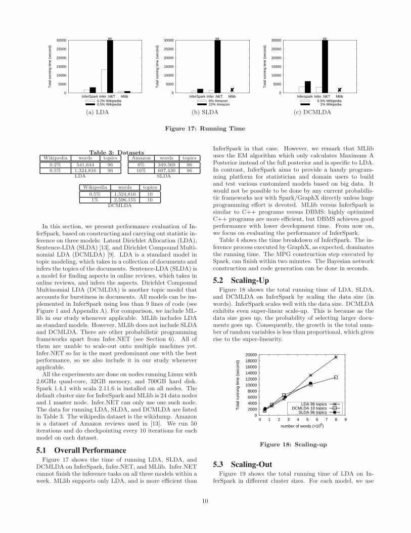
Figure 17: Running Time

Table 3: DatasetsWikipedia words topics

0.2% 541,644 960.5% 1,324,816 96

LDA

Amazon words topics

6% 349,569 9610% 607,430 96

SLDA

Wikipedia words topics

0.5% 1,324,816 101% 2,596,155 10

DCMLDA

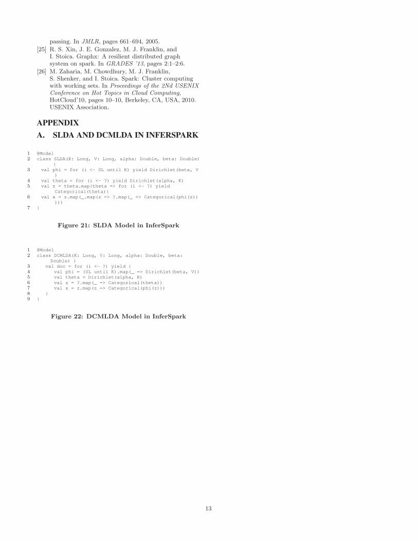
In this section, we present performance evaluation of In-ferSpark, based on constructing and carrying out statistic in-ference on three models: Latent Dirichlet Allocation (LDA),Sentence-LDA (SLDA) [13], and Dirichlet Compound Multi-nomial LDA (DCMLDA) [9]. LDA is a standard model intopic modeling, which takes in a collection of documents andinfers the topics of the documents. Sentence-LDA (SLDA) isa model for finding aspects in online reviews, which takes inonline reviews, and infers the aspects. Dirichlet CompoundMultinomial LDA (DCMLDA) is another topic model thataccounts for burstiness in documents. All models can be im-plemented in InferSpark using less than 9 lines of code (seeFigure 1 and Appendix A). For comparison, we include ML-lib in our study whenever applicable. MLlib includes LDAas standard models. However, MLlib does not include SLDAand DCMLDA. There are other probabilistic programmingframeworks apart from Infer.NET (see Section 6). All ofthem are unable to scale-out onto multiple machines yet.Infer.NET so far is the most predominant one with the bestperformance, so we also include it in our study wheneverapplicable.

All the experiments are done on nodes running Linux with2.6GHz quad-core, 32GB memory, and 700GB hard disk.Spark 1.4.1 with scala 2.11.6 is installed on all nodes. Thedefault cluster size for InferSpark and MLlib is 24 data nodesand 1 master node. Infer.NET can only use one such node.The data for running LDA, SLDA, and DCMLDA are listedin Table 3. The wikipedia dataset is the wikidump. Amazonis a dataset of Amazon reviews used in [13]. We run 50iterations and do checkpointing every 10 iterations for eachmodel on each dataset.

5.1 Overall PerformanceFigure 17 shows the time of running LDA, SLDA, and

DCMLDA on InferSpark, Infer.NET, and MLlib. Infer.NETcannot finish the inference tasks on all three models within aweek. MLlib supports only LDA, and is more efficient than

InferSpark in that case. However, we remark that MLlibuses the EM algorithm which only calculates Maximum APosterior instead of the full posterior and is specific to LDA.In contrast, InferSpark aims to provide a handy program-ming platform for statistician and domain users to buildand test various customized models based on big data. Itwould not be possible to be done by any current probabilis-tic frameworks nor with Spark/GraphX directly unless hugeprogramming effort is devoted. MLlib versus InferSpark issimilar to C++ programs versus DBMS: highly optimizedC++ programs are more efficient, but DBMS achieves goodperformance with lower development time. From now on,we focus on evaluating the performance of InferSpark.

Table 4 shows the time breakdown of InferSpark. The in-ference process executed by GraphX, as expected, dominatesthe running time. The MPG construction step executed bySpark, can finish within two minutes. The Bayesian networkconstruction and code generation can be done in seconds.

5.2 Scaling-UpFigure 18 shows the total running time of LDA, SLDA,

and DCMLDA on InferSpark by scaling the data size (inwords). InferSpark scales well with the data size. DCMLDAexhibits even super-linear scale-up. This is because as thedata size goes up, the probability of selecting larger docu-ments goes up. Consequently, the growth in the total num-ber of random variables is less than proportional, which givesrise to the super-linearity.

0

2000

4000

6000

8000

10000

12000

14000

16000

18000

20000

0 1 2 3 4 5 6 7 8 9

Tot

al r

unni

ng ti

me

(sec

ond)

number of words (×106)

LDA 96 topicsDCMLDA 10 topics

SLDA 96 topics

Figure 18: Scaling-up

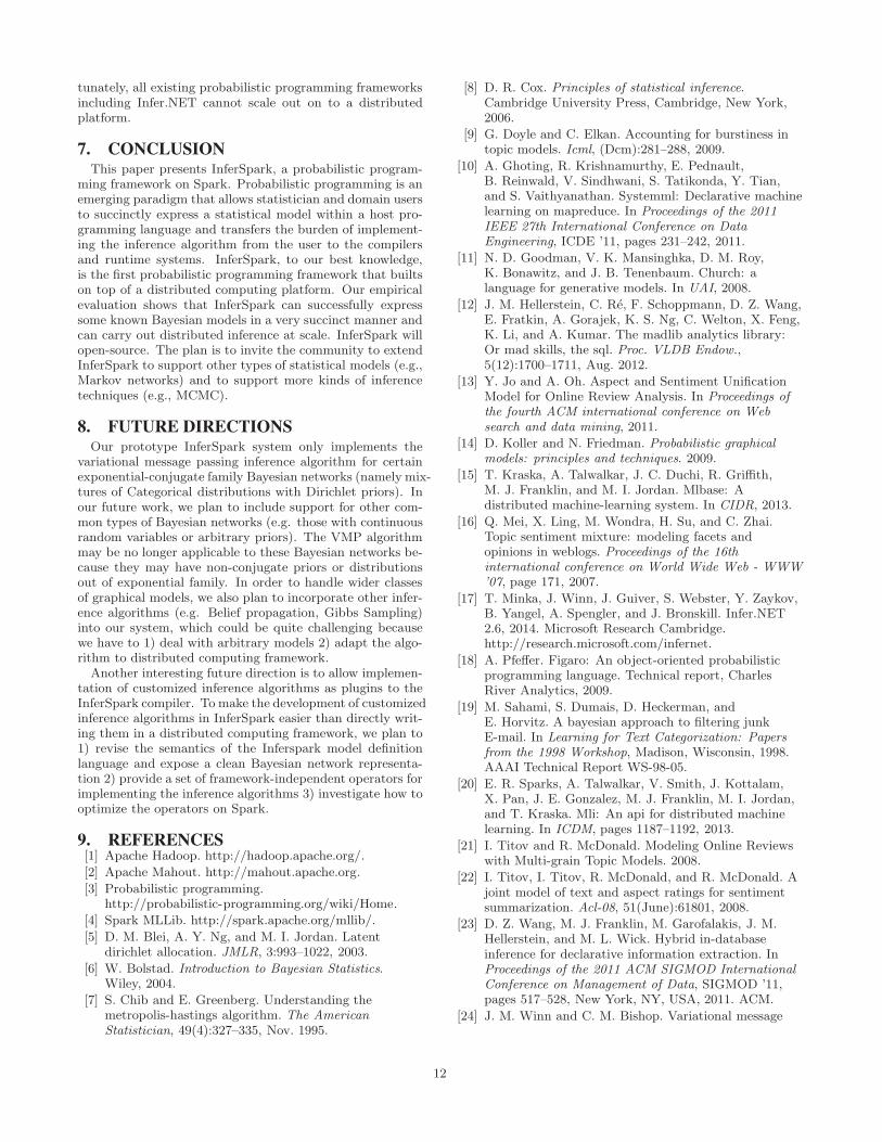
5.3 Scaling-OutFigure 19 shows the total running time of LDA on In-

ferSpark in different cluster sizes. For each model, we use

10

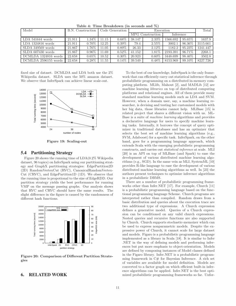
Table 4: Time Breakdown (in seconds and %)Model B.N. Construction Code Generation Execution Total

MPG Construction Inference

LDA 541644 words 21.911 1.34% 11.15 0.68% 38.147 2.33% 1566.692 95.65% 1637.9LDA 1324816 words 21.911 0.70% 12.25 0.39% 79.4 2.55% 3002.1 96.36% 3115.661SLDA 349569 words 21.867 1.76% 11.05 0.89% 26.33 2.12% 1182.2 95.23% 1241.447SLDA 607430 words 21.867 0.96% 11.69 0.52% 41.152 1.81% 2193.391 96.71% 2268.1DCMLDA 1324816 words 22.658 0.65% 10.52 0.30% 20.923 0.60% 3448.699 98.46% 3502.8DCMLDA 2596155 words 22.658 0.28% 11.55 0.14% 39.549 0.48% 8153.969 99.10% 8227.726

fixed size of dataset. DCMLDA and LDA both use the 2%Wikipedia dataset. SLDA uses the 50% amazon dataset.We observe that InferSpark can achieve linear scale-out.

4000

5000

6000

7000

8000

9000

10000

11000

12000

13000

14000

24 36 48

Tot

al r

unni

ng ti

me

(sec

ond)

number of nodes

LDADCMLDA

SLDA

Figure 19: Scaling-out

5.4 Partitioning StrategyFigure 20 shows the running time of LDA(0.2% Wikipedia

dataset, 96 topics) on InferSpark using our partitioning strat-egy and GraphX partitioning strategies: EdgePartition2D(2D) RandomVertexCut (RVC), CanonicalRandomVertex-Cut (CRVC), and EdgePartition1D (1D). We observe thatthe running time is propotional to the size of EdgeRDD. Ourpartition strategy yields the best performance for runningVMP on the message passing graphs. Our analysis showsthat RVC and CRVC should have the same results. Theslight difference in the figure is caused by the randomness ofdifferent hash functions.

0

2000

4000

6000

8000

10000

12000

14000

16000

18000

20000

InferSpark 2D RVC CRVC 1D 0

10

20

30

40

50

60

70

80

90

Tot

al r

unni

ng ti

me

(sec

ond)

Edg

eRD

D s

ize

(GB

)

partition strategy

timeEdgeRDD size

Figure 20: Comparison of Different Partition Strate-gies

6. RELATED WORK

To the best of our knowledge, InferSpark is the only frame-work that can efficiently carry out statistical inference throughprobabilistic programming on a distributed in-memory com-puting platform. MLlib, Mahout [2], and MADLib [12] aremachine learning libraries on top of distributed computingplatforms and relational engines. All of them provide manystandard machine learning models such as LDA and SVM.However, when a domain user, say, a machine learning re-searcher, is devising and testing her customized models withher big data, those libraries cannot help. MLBase [15] isrelated project that shares a different vision with us. ML-Base is a suite of machine learning algorithms and providesa declarative language for users to specify machine learn-ing tasks. Internally, it borrows the concept of query opti-mizer in traditional databases and has an optimizer thatselects the best set of machine learning algorithms (e.g.,SVM, Adaboost) for a specific task. InferSpark, on the otherhand, goes for a programming language approach, whichextends Scala with the emerging probabilistic programmingconstructs, and carries out statistical inference at scale. MLI[20] is an API on top of MLBase (and Spark) to ease thedevelopment of various distributed machine learning algo-rithms (e.g., SGD). In the same vein as MLI, SystemML [10]provides R-like language to ease the development of variousdistributed machine learning algorithms as well. In [23] theauthors present techniques to optimize inference algorithmsin a probabilistic DBMS.

There are a number of probabilistic programming frame-works other than Infer.NET [17]. For example, Church [11]is a probabilistic programming language based on the func-tional programming language Scheme. Church programs areinterpreted rather than compiled. Random draws from abasic distribution and queries about the execution trace aretwo additional type of expressions. A Church expressiondefines a generative model. Queries of a Church expres-sion can be conditioned on any valid church expressions.Nested queries and recursive functions are also supportedby Church. Church supports stochastic-memoizer which canbe used to express nonparametric models. Despite the ex-pressive power of Church, it cannot scale for large datasetand models. Figaro is a probabilistic programming languageimplemented as a library in Scala [18]. It is similar to Infer.NET in the way of defining models and performing infer-ences but put more emphasis to object-orientation. Modelsare defined by composing instances of Model classes definedin the Figaro library. Infer.NET is a probabilistic program-ming framework in C# for Bayesian Inference. A rich setof variables are available for model definition. Models areconverted to a factor graph on which efficient built-in infer-ence algorithms can be applied. Infer.NET is the best opti-mized probabilistic programming frameworks so far. Unfor-

11

tunately, all existing probabilistic programming frameworksincluding Infer.NET cannot scale out on to a distributedplatform.

7. CONCLUSIONThis paper presents InferSpark, a probabilistic program-

ming framework on Spark. Probabilistic programming is anemerging paradigm that allows statistician and domain usersto succinctly express a statistical model within a host pro-gramming language and transfers the burden of implement-ing the inference algorithm from the user to the compilersand runtime systems. InferSpark, to our best knowledge,is the first probabilistic programming framework that builtson top of a distributed computing platform. Our empiricalevaluation shows that InferSpark can successfully expresssome known Bayesian models in a very succinct manner andcan carry out distributed inference at scale. InferSpark willopen-source. The plan is to invite the community to extendInferSpark to support other types of statistical models (e.g.,Markov networks) and to support more kinds of inferencetechniques (e.g., MCMC).

8. FUTURE DIRECTIONSOur prototype InferSpark system only implements the

variational message passing inference algorithm for certainexponential-conjugate family Bayesian networks (namely mix-tures of Categorical distributions with Dirichlet priors). Inour future work, we plan to include support for other com-mon types of Bayesian networks (e.g. those with continuousrandom variables or arbitrary priors). The VMP algorithmmay be no longer applicable to these Bayesian networks be-cause they may have non-conjugate priors or distributionsout of exponential family. In order to handle wider classesof graphical models, we also plan to incorporate other infer-ence algorithms (e.g. Belief propagation, Gibbs Sampling)into our system, which could be quite challenging becausewe have to 1) deal with arbitrary models 2) adapt the algo-rithm to distributed computing framework.

Another interesting future direction is to allow implemen-tation of customized inference algorithms as plugins to theInferSpark compiler. To make the development of customizedinference algorithms in InferSpark easier than directly writ-ing them in a distributed computing framework, we plan to1) revise the semantics of the Inferspark model definitionlanguage and expose a clean Bayesian network representa-tion 2) provide a set of framework-independent operators forimplementing the inference algorithms 3) investigate how tooptimize the operators on Spark.

9. REFERENCES[1] Apache Hadoop. http://hadoop.apache.org/.

[2] Apache Mahout. http://mahout.apache.org.

[3] Probabilistic programming.http://probabilistic-programming.org/wiki/Home.

[4] Spark MLLib. http://spark.apache.org/mllib/.

[5] D. M. Blei, A. Y. Ng, and M. I. Jordan. Latentdirichlet allocation. JMLR, 3:993–1022, 2003.

[6] W. Bolstad. Introduction to Bayesian Statistics.Wiley, 2004.

[7] S. Chib and E. Greenberg. Understanding themetropolis-hastings algorithm. The American

Statistician, 49(4):327–335, Nov. 1995.

[8] D. R. Cox. Principles of statistical inference.Cambridge University Press, Cambridge, New York,2006.

[9] G. Doyle and C. Elkan. Accounting for burstiness intopic models. Icml, (Dcm):281–288, 2009.

[10] A. Ghoting, R. Krishnamurthy, E. Pednault,B. Reinwald, V. Sindhwani, S. Tatikonda, Y. Tian,and S. Vaithyanathan. Systemml: Declarative machinelearning on mapreduce. In Proceedings of the 2011

IEEE 27th International Conference on Data

Engineering, ICDE ’11, pages 231–242, 2011.

[11] N. D. Goodman, V. K. Mansinghka, D. M. Roy,K. Bonawitz, and J. B. Tenenbaum. Church: alanguage for generative models. In UAI, 2008.

[12] J. M. Hellerstein, C. Re, F. Schoppmann, D. Z. Wang,E. Fratkin, A. Gorajek, K. S. Ng, C. Welton, X. Feng,K. Li, and A. Kumar. The madlib analytics library:Or mad skills, the sql. Proc. VLDB Endow.,5(12):1700–1711, Aug. 2012.

[13] Y. Jo and A. Oh. Aspect and Sentiment UnificationModel for Online Review Analysis. In Proceedings of

the fourth ACM international conference on Web

search and data mining, 2011.

[14] D. Koller and N. Friedman. Probabilistic graphical

models: principles and techniques. 2009.

[15] T. Kraska, A. Talwalkar, J. C. Duchi, R. Griffith,M. J. Franklin, and M. I. Jordan. Mlbase: Adistributed machine-learning system. In CIDR, 2013.

[16] Q. Mei, X. Ling, M. Wondra, H. Su, and C. Zhai.Topic sentiment mixture: modeling facets andopinions in weblogs. Proceedings of the 16th

international conference on World Wide Web - WWW

’07, page 171, 2007.

[17] T. Minka, J. Winn, J. Guiver, S. Webster, Y. Zaykov,B. Yangel, A. Spengler, and J. Bronskill. Infer.NET2.6, 2014. Microsoft Research Cambridge.http://research.microsoft.com/infernet.

[18] A. Pfeffer. Figaro: An object-oriented probabilisticprogramming language. Technical report, CharlesRiver Analytics, 2009.

[19] M. Sahami, S. Dumais, D. Heckerman, andE. Horvitz. A bayesian approach to filtering junkE-mail. In Learning for Text Categorization: Papers

from the 1998 Workshop, Madison, Wisconsin, 1998.AAAI Technical Report WS-98-05.

[20] E. R. Sparks, A. Talwalkar, V. Smith, J. Kottalam,X. Pan, J. E. Gonzalez, M. J. Franklin, M. I. Jordan,and T. Kraska. Mli: An api for distributed machinelearning. In ICDM, pages 1187–1192, 2013.

[21] I. Titov and R. McDonald. Modeling Online Reviewswith Multi-grain Topic Models. 2008.

[22] I. Titov, I. Titov, R. McDonald, and R. McDonald. Ajoint model of text and aspect ratings for sentimentsummarization. Acl-08, 51(June):61801, 2008.

[23] D. Z. Wang, M. J. Franklin, M. Garofalakis, J. M.Hellerstein, and M. L. Wick. Hybrid in-databaseinference for declarative information extraction. InProceedings of the 2011 ACM SIGMOD International

Conference on Management of Data, SIGMOD ’11,pages 517–528, New York, NY, USA, 2011. ACM.

[24] J. M. Winn and C. M. Bishop. Variational message

12

passing. In JMLR, pages 661–694, 2005.

[25] R. S. Xin, J. E. Gonzalez, M. J. Franklin, andI. Stoica. Graphx: A resilient distributed graphsystem on spark. In GRADES ’13, pages 2:1–2:6.

[26] M. Zaharia, M. Chowdhury, M. J. Franklin,S. Shenker, and I. Stoica. Spark: Cluster computingwith working sets. In Proceedings of the 2Nd USENIX

Conference on Hot Topics in Cloud Computing,HotCloud’10, pages 10–10, Berkeley, CA, USA, 2010.USENIX Association.

APPENDIX

A. SLDA AND DCMLDA IN INFERSPARK

1 @Model

2 class SLDA(K: Long, V: Long, alpha: Double, beta: Double)

{

3 val phi = for (i <- 0L until K) yield Dirichlet(beta, V

)

4 val theta = for (i <- ?) yield Dirichlet(alpha, K)

5 val z = theta.map{theta => for (i <- ?) yield

Categorical(theta)}

6 val x = z.map(_.map(z => ?.map(_ => Categorical(phi(z))

)))

7 }

Figure 21: SLDA Model in InferSpark

1 @Model

2 class DCMLDA(K: Long, V: Long, alpha: Double, beta:

Double) {

3 val doc = for (i <- ?) yield {

4 val phi = (0L until K).map(_ => Dirichlet(beta, V))

5 val theta = Dirichlet(alpha, K)

6 val z = ?.map(_ => Categorical(theta))

7 val x = z.map(z => Categorical(phi(z)))

8 }

9 }

Figure 22: DCMLDA Model in InferSpark

13