q1899

DOCIKETED

;'5 MAP, -3 P'n 14: ()3

.. '1 -'- ~ ir F C >,

U.S. NUCLEAR REMILATORY COMMIS$IO

DocwNo. 70- V103nHL Of cwa E&1&ZLOFFERED by, Applkcant/Uensee

NRC staff_______

X)ENTnF)ED on 412~ Lo-witness/Panel__________ rAabonThlcmn ~)MJTTE) REJECTED WMID4RAWNW

Q QAG

27 r

infiltration Rates ThroughLandfill Liners

February 1998

Robert J. Murphy, Ph.DAnd

Erik Garwell

University of South Florida

State University System of FloridaFLORIDA CENTEREMN

FORSOLD AD AZARDOUS WASTE MANAGEMNFOR SOLID AND H2 NW 13 Street, Suite DGainesville, FL 32609

Report #97-11

ie lk--.,c-L

C)

Infiltration Rates Through Landfill Liners

Robert J. MurphyErik J. Garwell

University of South FloridaDept. of Environmental and Civil Engineering

4202 East Fowler AvenueTampa, Florida 33620

(813)-974-5815

February 27, 1998

Table Of Contents

List of Figures iv

List of Tables v

List of Abbreviations vi

Key Words viii

Abstract ix

Executive Summary x

1. Introduction 1

2. Landfill Liner Regulations and Requirements 4

2.1 Major Legislation for Solid Waste Management 4

2.2 Federal Agencies Involved with Solid Waste Management 5

2.3 Federal Landfill Final Cover Requirements 6

2.4 Florida Landfill Final Cover Requirements 6

2.5 Landfill Final Covers 8

3. Landfill Systems Flow Models 10

3.1 Chemicals, Runoff, and Erosion from Agricultural Management 11Systems (CREAMS)

3.2 Hydrologic Simulation on Solid Waste Disposal Sites (HSSWDS) 11

3.3 Unsaturated Groundwater Flow Model (UNSATID) 11

3.4 Hydrologic Evaluation of Landfill Performance (HELP) Model 12

3.5 SOILINER 12

3.6 Unsaturated Soil Water and Heat Flow Model (UNSAT-H) 13Version 2.0

3.7 FULFILL 13

3.8 Model Investigation of Landfill Leachate (MILL) 133.9 The Flow Investigation for Landfill Leachate (FILL) 13

3.10 Landfill Liner System Flow Model 14

3.11 Finite-Element Model 14

4. HELP Model Evaluation 154.1 HELP Model, Version 1 15

4.1.1 Version 1 Studies 16

4.2 HELP Model, Version 2 18

4.2.1 Version 2 Studies 18

4.3 HELP Model, Version 3 194.3.1 Version 3 Studies 194.3.2 Advantages of HELP 204.3.3 Assumptions and Limitations of HELP 21

ii

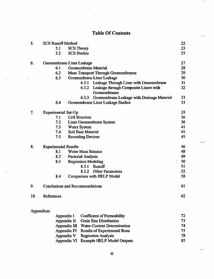
Table Of Contents

5. SCS Runoff Method 225.1 SCS Theory 235.2 SCS Studies 25

6. Geomembrane Liner Leakage 276.1 Geomembrane Material 286.2 Mass Transport Through Geomembranes 296.3 Geomembrane Liner Leakage 30

6.3.1 Leakage Through Liner with Geomembrane 316.3.2 Leakage through Composite Liners with 32

Geomembranes6.3.3 Geomembrane Leakage with Drainage Material 33

6.4 Geomembrane Liner Leakage Studies 33

7. Experimental Set-Up 357.1 Cell Structure 367.2 Liner Geomembrane System 367.3 Water System 417.4 Soil Base Material 417.5 Recording Devices 45

8. Experimental Results 468.1 Water Mass Balance 488.2 Factorial Analysis 498.3 Regression Modeling 50

8.3.1 Runoff 518.3.2 Other Parameters 52

8.4 Comparison with HELP Model 58

9. Conclusions and Recommendations 61

10. References 62

AppendicesAppendix I Coefficient of Permeability 72Appendix II Grain Size Distribution 73Appendix ml Water-Content Determination 74Appendix IV Results of Experimental Runs 75Appendix V Regression Analysis 78Appendix VI Example HELP Model Outputs 85

iii

List of Figures

Figure 1 Recommended Surface Barrier Cross-Section for Hazardous-Waste 7and Solid-Waste Landfills

Figure 2 Isometric View of the Experimental Cell Base Structure 37

Figure 3 Exploded View of the Experimental Cell Base Structure 38

Figure 4 Adjustable Experimental Framed Floor 39

Figure 5 Experimental Liner System Plan View 39

Figure 6 Experimental Liner System Section A-A 40

Figure 7 Experimental Collection Points 40

Figure 8 Water System Support Frame 42

Figure 9 Mister Support System 43

Figure 10 Water System Plan View in the Experimental Cell 43

Figure 11 Water System Percent Distribution in the Experimental Cell 44

Figure 12 Experimental Soil Matrix 44

Figure 13 Runoff Collection off of the Experimental Cell 45

Figure 14 Runoff Flux vs. Storm Intensity 47

Figure 15 Residual Plots for Runoff Model (3-variables): (a) Hydraulic 54Conductivity (b) Storm Intensity, and (c) Slope

Figure 16 Line Fit Plots for Runoff Model (3-variables): (a) Hydraulic 55Conductivity (b) Storm Intensity, and (c) Slope

Figure 17 Residual Plots for Leakage Model (3-variable): (a) Hydraulic 56Conductivity (b) Storm Intensity, and (c) Slope

Figure 18 Line Fit Plots for Leakage Models: (a) Slope (3-variables) and 57(b) Slope (second model)

iv

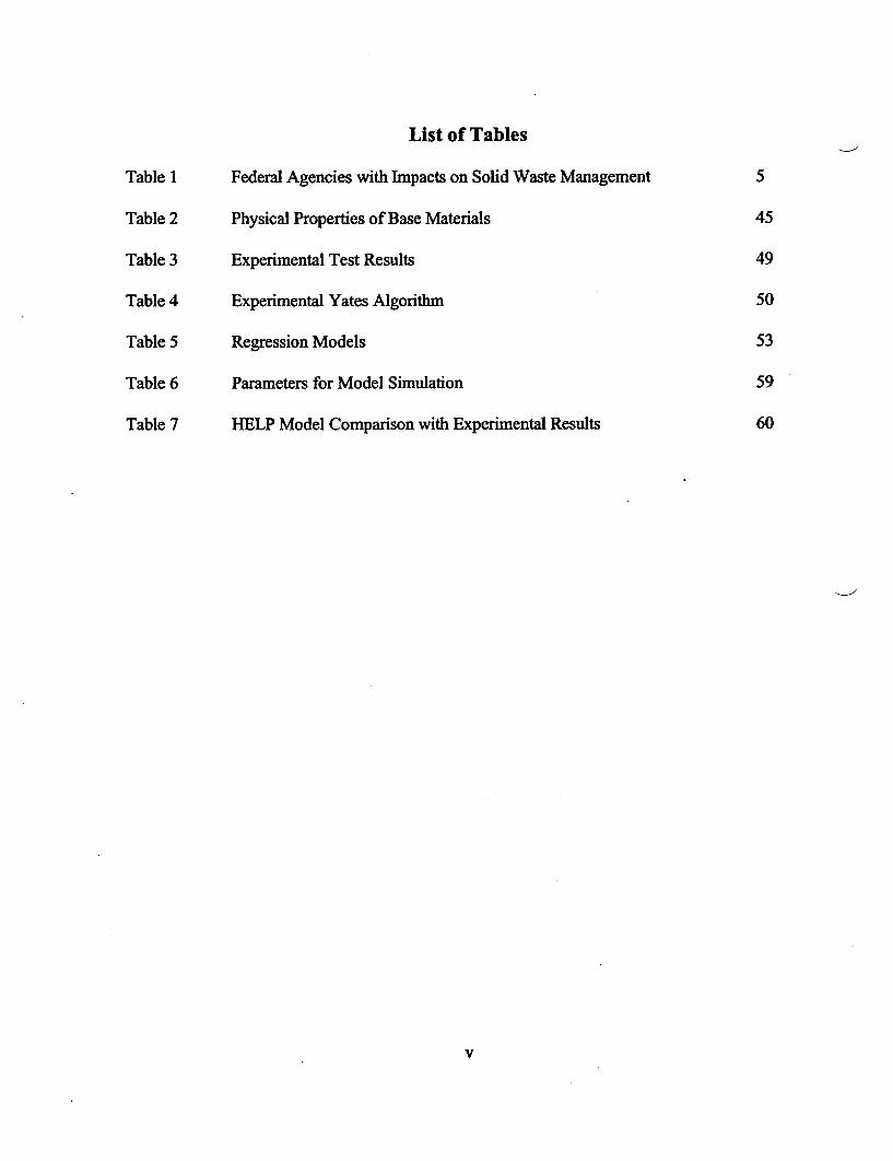
List of Tables

Table 1 Federal Agencies with Impacts on Solid Waste Management 5

Table 2 Physical Properties of Base Materials 45

Table 3 Experimental Test Results 49

Table 4 Experimental Yates Algorithm 50

Table 5 Regression Models 53

Table 6 Parameters for Model Simulation 59

Table 7 HELP Model Comparison with Experimental Results 60

v

List of Abbreviations

AMCBPNLCERCLACFRcmCNCoCPECPE-ACRCREAMSCSPEdDOCDODDOEDOTEIAEISEPAETF.A.C.FDEPFILLFMLftGPHGPMGSAHCHDPEHDPE-AHELPHEWhrHSSWDSIIDIIRinkg

Antecedent Moisture ConditionBattelle, Pacific Northwest LaboratoriesComprehensive Environmental Response, Compensation and Liability ActCode of Federal RegistryCentimetersCurve NumberEpichlorohydrin RubberChlorinated PolyethyleneChlorinated Polyethylene-AlloyEthylene-Propylene PolychloropreneChemicals, Runoff, and Erosion from Agricultural Management SystemsChlorosulfonated PolyethyleneDayDepartment of CommerceDepartment of DefenseDepartment of EnergyDepartment of TransportationEthylene Interpolymer AlloyEnvironmental Impact StatementEnvironmental Protection AgencyEvapotranspirationFlorida Administrative CodeFlorida Department Environmental ProtectionThe Flow Investigation for Landfill LeachateFlexible Membrane LinerFeetGallons Per HourGallons Per MinuteGeneral Services AdministrationHydraulic ConductivityHigh-Density PolyethyleneHigh Density Polyethylene-AlloyHydrologic Evaluation of Landfill PerformanceHealth, Education, and WelfareHourHydrologic Simulation on Solid Waste Disposal SitesInfiltrationStorm IntensityIsobutylene RubberInchesKilogram

vi

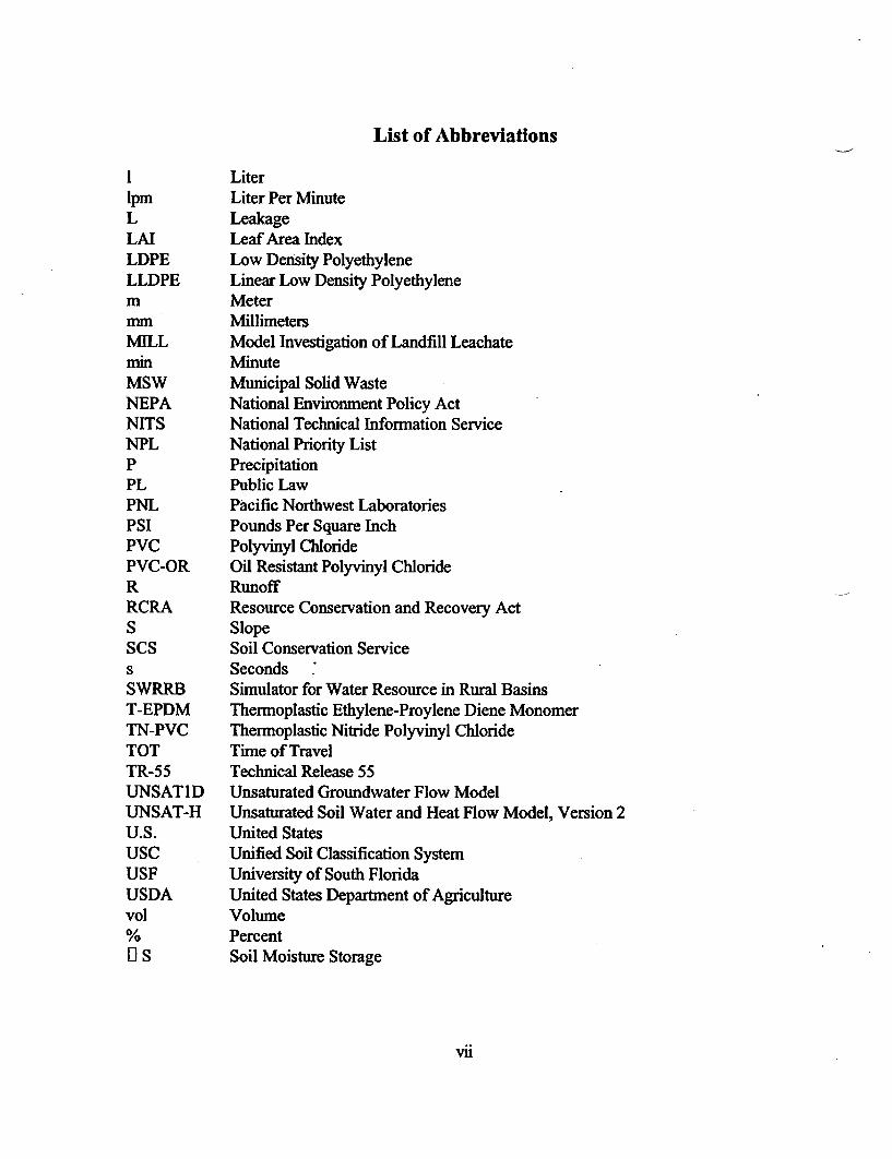
List of Abbreviations

1IpmLLAILDPELLDPEmmmMILLmmnMSWNEPANITSNPLPPLPNLPSIPVCPVC-ORRRCRASSCSs

SWRRBT-EPDMTN-PVCTOTTR-55UNSATIDUNSAT-HU.S.USCUSFUSDAvol

OS

LiterLiter Per MinuteLeakageLeaf Area IndexLow Density PolyethyleneLinear Low Density PolyethyleneMeterMillimetersModel Investigation of Landfill LeachateMinuteMunicipal Solid WasteNational Environment Policy ActNational Technical Information ServiceNational Priority ListPrecipitationPublic LawPacific Northwest LaboratoriesPounds Per Square InchPolyvinyl ChlorideOil Resistant Polyvinyl ChlorideRunoffResource Conservation and Recovery ActSlopeSoil Conservation ServiceSecondsSimulator for Water Resource in Rural BasinsThermoplastic Ethylene-Proylene Diene MonomerThermoplastic Nitride Polyvinyl ChlorideTime of TravelTechnical Release 55Unsaturated Groundwater Flow ModelUnsaturated Soil Water and Heat Flow Model, Version 2United StatesUnified Soil Classification SystemUniversity of South FloridaUnited States Department of AgricultureVolumePercentSoil Moisture Storage

vii

Key Words

Municipal Solid WasteLandfillRunoffInfiltrationLeakageRegression Modeling

vmi

Abstract

Predictive modeling involved with landfills requires an understanding of moisturemovement through final surface covers. An experimental study was undertaken to evaluate therunoff, infiltration, and leakage through a final surface cover liner system with a geomembraneand present predictive models The project's objectives included: assessment of applications ofcurrent liner technology and regulations, presentation of existing landfill flow models,identification of surface cover and geomembrane leakage mechanisms, presentation of results ofexperimental testing of a landfill topliner system, development of mathematical models tailored tolandfill final cover applications, and statistical evaluation of the models with the experimental data.

A total of 61 experimental runs were run from February to June 1997. The infiltration andleakage parameters were monitored although the primary interest was to evaluate the runoff.The objective of this experiment was to measure the moisture movement through the final coversystem when the liner is at field capacity. The average mass water balance for the experimentalsimulations ranged from 93.3% to 96.7%. The experimental data was converted from a massparameter to flux values, gallons per minute-acre, for a more descriptive output. Modeling therunoff flux was the principal result of the evaluation. The analysis used storm intensity, slope, andhydraulic conductivity parameters to predict the runoff flux values. A linear relationship wasclearly seen from the experimental data. The correlation coefficients for the two runoff modelsare .983 and .984, respectively, indicating an excellent data fit. A geomembrane leakage trend isapparent from the data analysis; as the slope increases the average leakage flux decrease.

The experimental runoff flux data was compared with default runoff predictions from theHydrologic Evaluation of Landfill Performance (HELP) model. The HELP model tends tounderpredict runoff for all simulations run on the experimental cell, which ultimately results in anoverprediction of infiltration. Underprediction of the runoff flux ranged from 8% to 24% for thesimulations. The HELP model runoff flux output is highly dependent on the soils hydraulicconductivity and moisture storage capacity. Predictions made with the HELP model are notnecessarily accurate, even when the input parameters have a high degree of precision.

ix

Executive Summary

Landfilling has been the most economical and environmentally accepted method of solidwaste disposal in the United States (US) and in the world. Implementation of waste reduction,recycling, and transformation technologies has decreased landfill burdens, but landfills remain animportant component of an integrated solid waste management strategy. A good final coversystem should be designed to reduce infiltration and ultimate leachate generation. Reduction ofinfiltration in a landfill is achieved through surface drainage and runoff with minimal erosion,transpiration, and restriction of percolation.

With the implementation of the Resource Conservation and Recovery Act (RCRA) 40CFR Part 258 or 'Subtitle D' regulations, maintenance, design, and final closure of landfillschanged. The regulations require the final cover be equal or better than the bottom liner system.This regulation has propelled synthetic materials to the forefront of liner systems.

Presently, the means to combat leachate migration to the surrounding subsurface andground water is to have an impermeable geomembrane liner encompassing the landfill. A linersystem using geomembrane material typically encloses the solid waste matrix in a single or doublegeomembrane liner. Geomembranes are engineered polymeric materials produced to be virtuallyimpermeable. Studies have shown that high-density polyethylene (HDPE) is the material ofchoice for a wide range of wastes typically encountered in landfill disposal facilities. Most doubleliner systems installed to date have developed a loss of integrity and are expected to producesome leakage through the liner material. Consequently, liner systems have been designed tocounteract the inability to construct a perfect liner. The objective is to design a combination ofvarious liner components into a liner system that will reduce the leakage rate into and fromlandfills.

Regulations require that post-closure care be conducted for 30 years or for a periodapproved by the state if the owner can demonstrate the reduced period is sufficient. Leachatetreatment and disposal are an inherent part of post-closure care. Currently, several models areused to predict moisture movement at solid waste disposal sites. A common deficiency inresearch on liner mechanisms has been the focus on the evaluation of the bottom liners. As aresult, there may be a lack of pertinent data on the final surface cover liner systems and howpercolation is affected by liner types. Most of the existing models have not been specificallydesigned to project infiltration of the caps and sideslopes of landfills, and most lack sufficientexperimental field data to support them.

This project advances the methods for determining runoff and infiltration rates generatedthrough final surface cover systems at landfills. The results of this project have led to a betterprojection of runoff and infiltration through final cover systems at landfills with synthetic linersystems. The project's objectives included:

x

[1 Assessment of applications of current liner technology and regulations;* Presentation of existing landfill flow models;* Identification of surface cover and geomembrane leakage mechanisms;* Presentation of results of experimental testing of a landfill topliner system;* Development of mathematical models tailored to landfill final cover applications;* Statistical evaluation of the mathematical models with experimental data.

Landfill literature has shown many landfill failures are attributed to insufficient surfacebarriers. Even in arid regions, over time, buried waste is vulnerable to transport via rainwaterpercolation, gas diffusion, erosion, and intrusion by plant roots, burring animals, and humans.Standard models and field tests of engineering covers designed to impede these pathwaysimplicitly and erroneously assume that surface barrier technology is well developed and works asexpected.

Landfill liner systems consist of a top and bottom liner. The top liner is designed to prevent orreduce the migration of precipitation into the waste. The bottom liner is designed to collect andremove leachate that may make its way through the system. Generally, bottom liners consist of aleachate collection system and liner. Leachate collected is drained from the liner to reduce fluidpressure on the liner. Many research efforts have been devoted to predicting landfill moisture flow.Several methods and computer models have been developed to deal with the unique conditions of alandfill. These numeric models fall into the general categories of deterministic water balance methodsand finite-difference methods. Landfill flow modeling consists of predicting the runoff, infiltration, andleakage rate of a system.

The water balance methods are based on procedures developed by C.W. Thorthwaite in thesoil and water conservation field. Since his work many research efforts have developed the waterbalance equations in the last 40 years. These qualitative water balance models consider the landfill a"black box," requiring a material balance of water flow into and out of the system. The water balancemodels have been used extensively in predicting leachate quantity and aiding design of landfills.

The most widely used predictive water balance landfill infiltration model is the HydrologicEvaluation of Landfill Performance (HELP) model. HELP is a quasi-two-dimensional, deterministicwater balance model that estimates daily water movement through landfills. Water migrating throughlandfill barrier layers may stress liner systems and possibly lead to a breach. Although HELP is usedextensively by regulatory agencies there are few verifications or investigations of the predictive abilitiesof the model. HELP estimates runoff, infiltration, evapotranspiration, drainage, leachate collection,and liner leakage. The HELP model has been shown to provide reasonable predictions of infiltrationof moisture movement through landfills. However, the model's theoretically based algorithms andlimited verification studies present several limitations: the Soil Conservation Service (SCS) equationswith the HELP infiltration approach may carry the method beyond the data on which it was based andproduce erroneous results, the dominant flow mechanism is assumed to be porous media flow, wherethe lateral moisture movement is only allowed in drainage layers, and the effects of alternative slopes ansideslopes cannot be modeled.

xi

Surface water infiltration is perhaps the largest contributing factor of leachate production insanitary landfills. It may directly affect moisture content of the landfill system. Runoff begins whenthe rainfall intensity exceeds the infiltration capacity of the soil matrix. Factors affecting surface runoffare surface topography, cover material, vegetation, permeability, moisture condition, and precipitation.The SCS method can be summarized as a relationship of soil depth and runoff depth.. Many factorsinfluence infiltration including rainfall patterns, initial soil moisture, tillage practice, physical soilproperties, and influences of vegetation roots and stems. Factors that influence overland flowattenuation include surface roughness, storage, slope, size of watershed, and rate of precipitation.

The principal application of the SCS method is estimating runoff in flood hydrographs.Rainfall data used in the development generally is from ungauged watersheds. The relationshipexcludes time as a variable. Runoff amounts for specific time increments of a storm may be estimated.The method was intended as a design procedure for SCS personnel in evaluating watershed responsefor SCS projects, and it has since been adopted for use by various government agencies including theEnvironmental Protection Agency.

Currently, geomembranes are a widely used material in final surface cover design. Manyfactors contribute to leakage, including the geometry, configuration, and cross-sections of the landfill.The primary mechanisms of leakage through landfill geomembrane liners are fluid permeation throughthe undamaged geomembrane cover, and fluid flow through geomembrane defects and holes. Leakagethrough a geomembrane hole is primarily dependent on three factors: (1) area of hole; (2) hydraulicconductivity of layer above and/or below the geomembrane, and (3) liquid head over the liner. Evenwith the best quality control during installation of geomembrane liners one can expect I to 2 defectsper acre (3 to 5 defects per hectare).

The ability of a final cover system to prevent infiltration into underlying material is largelydetermined by the effectiveness of the final cover system. The surface layer is the upper soil layer thatintercepts rainfall and removes a segment as surface runoff. Part of the rainfall that infiltrates theupper soil layer then penetrates the infiltration layer. A large part of the water that migrates from theupper soil layer is expected to drain by gravity, moving along the geomembrane to a drainagecollection point Finally, some amount of the water will flow through the geomembrane liner asleakage, but this will be much less than runoff and infiltration.

An experimental cell was designed to simulate a landfill cover for a variety of short-term high-intensity storm events. The cell consisted of a base structure built of pressure-treated wood, ageomembrane liner system, a simulated rainfall system, soil cover material, and recording devices. Thecell was built approximately eight feet (2.44 m) in length, two feet (0.61 m) in width, and three feet(0.92 m) in height. The liner system was designed to simulate a final cover system constructed with60-mil high density polyethylene geomembrane that complies with the State of Florida landfill designstandards. A total of 61 experimental runs were made from February to June 1997. The infiltrationand leakage parameters were monitored, although the primary interest was to evaluate the runoff. Theexperimental results are presented as follows: water mass balance across the experimental apparatus;

x.i

factorial analysis of the main effects and interactions of the principal variables; statistical modeling of

the system using regression analysis; and comparison of data to the HELP model.

The water balance of the landfill cover may be segregated into six components: precipitation(P), runoff (R), infiltration (1), evapotranspiration (ET), soil moisture storage (O S), and Leakage (L).These parameters must be properly estimated to balance the water in the cover system. The water

balance methods are used to perform a mass balance on the experimental system. These parameterswere addressed in the experiment as follows: precipitation is known, runoff, infiltration, and leakage

was collected and measured, evapotranspiration is insignificant due to the short duration of the storm

event, and soil moisture storage is known by using a soil matrix at field capacity.

As was noted from the literature review of landfill surface runoff modeling, predicting short-

duration, high-intensity storm events needed a more thorough assessment A 30-minute duration

storm event was developed to assess runoff in storm simulations. The time increment is extensive

enough to produce runoff, infiltration, and leakage with the exposed soil at field capacity moisturecontent The primary parameters chosen for evaluation were landfill slope, storm intensity, and

hydraulic conductivity of the soil matrix. An experimental statistical factorial design was developed toevaluate these parameters and potential interactions.

Factorial designs facilitate the evaluation of the interactions of variables and thus assist the

process of model building. These experimental designs provide estimates of the "effects" of theinteractions, while assuring that such interactions are not experimental errors. In statistical factorial

designs, high and low values of the parameters maybe used to set up a matrix. In this experiment the

storm events were a 2-year frequency event and a 10-year event, slopes were evaluated at 2%, 5%,

and I10%, and the hydraulic conductivity of the upper soil layers used were 6.5 x IV- inch/sec (1.6 x 104 cmn/s) and 7.5 x 106 inch/sec (1.9 x 1IO cmn/s). Simulations were performed on all combinations of

the primary variables.

The purpose of the factorial design matrix was to statistically test as many parameters aspossible simultaneously. A matrix was used to analyze the runoff data using Yates algorithmcalculations. The high estimates of the effects storm intensity and hydraulic conductivity indicated they

are the major factors affecting the system and, since the interaction between the two was low, were

acting independently of each other. The slope parameter appears to have minimal affect on the runoff

flux. Consequently, it was concluded that the main independent variables that affect runoff are storm

intensity and soil hydraulic conductivity, whereas the slope of the soil surface was not a significantfactor within the range of 2% to 10%.

The average mass balance for the experimental final cover system ranged from 93.3% to

96.7%. The low standard deviations for average runoff flux and the high closure rate indicated good

reliability of the data. The experimental data was converted from a mass parameter to flux values,

gallons per minute-acre, for a more descriptive output Modeling the runoff was the principal concernand used storm intensity, slope, and hydraulic conductivity to predict runoff flux values. A linear

relationship was clearly seen from the experimental data. The correlation coefficients for the two

x7

runoff models are .983 and .984, respectively, indicating and excellent data fit. Storm intensity andhydraulic conductivity clearly have a good linear fit, but the slope parameter obviously has nosignificant impact. The hydraulic conductivity evaluation may be limited due to the constricted rangeof this variable (2 levels) in this study. Although two soil hydraulic conductivities were explored in thestudy, the second soil matrix was possibly too impermeable to provide reliable data. Two leakagemodels were presented: a 3-variable model and a 2-variable model. Data trends for the leakage modelswere difficult to predict due to the second soil profile producing minimal leakage, which effectivelygave only two parameters to evaluate. A leakage trend appears to exit; as the slope increased theleakage flux decreased.

The results of this study serve to identify an alternative approach to predicting surface runofffrom closed landfills. Consequently, the design of surface runoff collection/storage requirements canbe more simply projected within the range of the variables evaluated in this study. Generally, thescenario for such predictions is encompassed in the experiments and the resultant regression model'shave been developed. Further, the experimental results confirm previous evaluations of the HELPmodels underprediction of surface runoff from landfills. It is also significant that the experimentalresults demonstrated that, at a surface slope of I10%, the effects of leachate leakage through holes inthe underlying surface geomembrane liner are minimized. Obviously, such a slope mitigates thecreation of sufficient static head in the soil above the liner to facilitate leachate through thegeomembrane liner. These results may also be translated into the effects of slope on the bottom linerleakage rates in landfills (i.e., a slope of 10% on the bottom liner may inhibit leakage in the bottom linersystem).

The experimental runoff flux data was compared with default runoff predictions from theHELP model. The HELP model tends to underpredict runoff for all simulations run on theexperimental cell, which ultimately results in an overprediction of infiltration. Underprediction of therunoff flux ranged from 8% to 24% for the simulations. The HELP model runoff flux output is highlydependent on the soils hydraulic conductivity and moisture storage capacity. Prediction made with the:HELP model are not necessarily accurate, even when the input parameters have a high degree ofprecision.

Follow-up research should be performed using other ranges of the parameters selected for thisstudy. This is especially significant for additional soil material with a broad range of hydraulicconductivity, which would enhance the leakage models. A single or a set of regression models shouldbe developed specifically designed for landfill use. Further, based on the literature review, capillarybarriers need to be evaluated for their ability to impede infiltration. Reduction of leakage with thesecapillary systems may be possible, but current experimental field data is not sufficient to substantiate.

xiv

1. INTRODUCTION

Landfilling has been the most economical and environmentally accepted method of solid wastedisposal in the U.S. and in the world (rchobanoglous et al., 1993). Implementation of wastereduction, recycling, and transformation technologies has decreased landfill burdens but landfills remainan important component of an integrated solid waste management strategy. In Florida, an estimated69% of municipal solid waste (MSW) generated is landfilled (Murphy and Batiste, 1991). Leachateproduced in these landfills are the result of moisture acting as a solvent seeping through the landfill cellsand enhancing solid waste decomposition. Depending on the type of material deposited in the landfill,this leachate may be considered contaminated. A good final cover system should be designed toreduce infiltration and ultimate leachate generation.

Generally the best approach to impede leachate generation is the use of an impermeablegeosynthetic in the final surface cover. The purposes of final cover systems in landfills are to reducethe infiltration of water from precipitation, limit the uncontrollable release of landfill gasses, reduce theproliferation of vectors, reduce potential fires, provide surface revegetation, and serve as a primaryelement in reclamation of the site (Tchobanoglous et al., 1993) Reduction of infiltration in a landfill isachieved through surface drainage and runoff with minimal erosion, transpiration, and restriction ofpercolation (EPA, 1992).

With the implementation of the Resource Conservation and Recovery Act (RCRA) 40 CFRPart 258 or 'Subtitle D' regulations in 1993, maintenance, design, and final closure of landfills changed.No longer was it acceptable to merely put MSW in a large excavation. The regulations require thefinal cover be equal or better than the bottom liner system. This regulation has propelled syntheticmaterials to the forefront of liner systems. Specifically, the post-closure criteria require a maintenanceand monitor period of 30 years and give guidelines for hydraulic barrier layers, vegetative layers, andhydrologic surface conditions. These liner systems need to be evaluated for the long term risk ofinfiltration.

Presently, the means to combat leachate migration to the surrounding subsurface and groundwater is to have an impermeable geomembrane liner encompassing the landfill. A liner system usinggeomembrane material typically, a single or double geomembrane liner, encloses the solid wastematrix. Geomembranes are engineered polymeric materials produced to be nearly impermeable.Studies have shown that high-density polyethylene (HDPE) is the material of choice for a wide rangeof wastes encountered in landfill disposal facilities (LaGrega et al., 1994). Most double liner systemsinstalled to date have developed a loss of integrity. This is verified with the detection of leachate in thesecondary leakage detection liner system. A study by Southeast Research Institute on 28geomembrane-lined storage facilities showed only two liner systems had no leaks. An average of 26.2leaks per 10,000 square meters was reported (Murphy and Borgmeyer, 1992).

Current knowledge concedes that the absolute leak-proof liner is improbable to accomplish.Accordingly, systems have been designed to compensate for the failure to produce an impermeableliner system. The objective is to design a liner system with a combination of various components that

1

reduce the leakage rate into and from landfills (Tedder, 1992). The leakage rate may be a result ofimperfect seaming, rips, punctures during installation, and failures that result from soil failures afterinstallation. The U.S. Office of Technical Assessment reported the three most common geomembraneliner failures are deficient seam welds, deformation due to poor liner subbase, and tears and puncturesoften caused by vehicles (Jayawickrama et al., 1988).

Whatever the cause, liners leak and require management. The cost of leachate management isestimated at $1.36/ton-year of the landfilled waste (Murphy and Batiste, 1991) and is incurred for thepost-closure period and possibly longer. There is a potential for continual leachate generation inlandfills. Cost and methods of treatment alternatives vary depending on quality and quantities of theleachate. It is important that leachate generation rates are correctly determined to design and projectthe cost of the treatment system.

Regulations require that post-closure care be conducted for 30 years or for a period approvedby the state if the owner can demonstrate the reduced period is sufficient (EPA, 1992). Leachatetreatment and disposal are an inherent part of post-closure care. Currently, several models are used topredict quantity of leachate generation at solid waste disposal sites as a function of water infiltrationand number of cells. Perhaps the best known is the water balance model, Hydrologic Evaluation ofLandfill Performance (HELP) (Schroeder et al., 1984a, 1984b). HELP was intended as a tool fordesigning new landfills, but is also used in estimating leachate generation. The HELP model may belimited in the application. For example, HELP may yield a zero result when given a proper mix oflandfill surface layers and their characteristics (Nixon, 1995). As noted earlier, this ideal result is notattainable in actual construction. To date, surface water hydrologic models and models designed todetermine leakage from the bottom liner have been used to calculate infiltration into the top liner.

A common deficiency in research on liner mechanisms has been the focus on the evaluation ofthe bottom liners. As a result, there may be a lack of pertinent data on the final surface cover linersystems and how percolation is affected by liner types. Most of the existing models have not beenspecifically designed to project infiltration of the caps and sideslopes of landfills, and most lacksufficient experimental field data to support them.

This project advances the methods for deternining runoff and infiltration rates generatedthrough final cover systems at landfills. The study at the University of South Florida (USF) included:

* Assessment of applications of current liner technology and regulations;* Evaluation of existing landfill flow models;* Identification of surface cover and geomembrane leakage mechanisms;* Presentation of results of experimental testing of a landfill topliner pilot scale system;* Development of experimental mathematical models specifically tailored to landfill final

cover applications;* Statistical evaluation of the mathematical models with experimental data.

2

The results of this project may lead to a better predictions of runoff, infiltration, and leakageflux through caps and side slopes of landfills with synthetic liner systems.

3

2. LANDFILL LINER REGULATIONS AND REQUIREMENTS

The solid waste burden on landfills will continue for years to come. Although legislation hasbeen enacted to direct a good portion of solid waste to recycling and reuse, landfills are still needed.Solid waste management is primarily affected by the federal legislative process. Most stategovernments adopt federal regulations as a minimum standard to their solid waste managementprograms. This chapter explains the major legislation of solid waste and federal and states guidelinespertinent to landfill final cover designs.

2.1 MAJOR LEGISLATION FOR SOLID WASTE MANAGEMENT

The federal government has provided impetus for solid waste management legislation thatbegan approximately 30 years ago. The first major legislation enacted was the Solid Waste DisposalAct, PL 89-272, of 1965. The law was intended to (Tchobanoglous et al., 1993):

El Promote solid waste management and resource recovery systems;[1 Provide technical and financial assistance in solid waste programs;[1 Promote research and development programs for improved solid waste management;[1 Provide guidelines for collection, transport, separation, recovery, and disposal systems;[1 Provide training grants for occupations involving solid waste management.

The National Environment Policy Act (NEPA) is a congressional law enacted in 1969. It gavethe public an opportunity to participate in the process by creating the Council of EnvironmentalQuality in the Office of the President. The council has the authority to force every federal agency tosubmit an Environmental Impact Statement (EIS) on every project. An EIS statement evaluates allpossible detrimental effects on the environment and must be prepared for solid waste facilities.

The Resource Recovery Act of 1970 changed the emphasis of management from disposal torecycling and reuse. Progress under the Resource Recovery Act prompted congress to pass theResource Conservation and Recovery Act (RCRA), in 1976. RCRA was the legal basis forimplementation of guidelines for solid waste storage, treatment, and disposal. The legislation includedboth hazardous and solid waste, later separated by the Environmental Protection Agency (EPA).RCRA has been amended often since its inception by various laws and currently major regulationsconcerning MSW landfills.

The Comprehensive Environmental Response, Compensation and Liability Act (CERCLA),PL 96-510, was enacted in 1980. CERCLA established a trust fund called "Superfund" that allowedan immediate response to problems at uncontrollable hazardous waste disposal sites. UncontrollableMSW landfills are facilities that have not operated or are not operating under RCRA permits.Uncontrolled landfills are subject to CERCLA. Reauthorization in 1986 extended the nation'scommitment to resolving past problems of mismanagement of hazardous waste. Over 32,000 siteshave been identified as potential hazardous waste sites, and 1183 sites are currently on the NationalPriority List (NPL) (Peters, 1992).

4

The Public Utility Regulation and Policy Act was enacted in 1981. This law directs public andprivate utilities to purchase power from waste-to-energy facilities and the manner in which utilities setprices.

MSW landfills today are subject to EPA regulations pursuant to 40 CFR Part 258, Subtitle Dof RCRA, released as final on October 9, 1991. The regulations strengthened the design requirementsfor new MSW landfills to nearly reflecting those of hazardous waste landfills. Under subtitle D, coverrequirements are based primarily on the hydraulic conductivity of the bottom liner (EPA, 1993).Existing MSW landfills were forced to make modifications to meet the new standards. Theregulations economically impacted almost every MSW landfill in the United States except thosealready operating under strict regulations.

Many other laws apply to the control of solid waste management. These include the NoisePollution and Abatement Act of 1970, which regulates the noise exposure to workers employed atsolid waste facilities. The Clean Air Act of 1970, PL 91-604, pertaining to dust, smoke, and gasdischarge from solid waste operations. Many states have adopted their own laws and have establishedagencies for the control of solid waste management.

2.2 FEDERAL AGENCIES INVOLVED WITH SOLID WASTE MANAGEMENT

Solid waste management has become a responsibility of many federal agencies due to thevarious laws, regulations, and executive orders in the past 30 years. Federal agencies interpret lawsand apply the minimum standards to be followed by all states. Some significant agencies and theirimpacts are presented in Table 1.

Table 1 Federal Agencies with Impacts on Solid Waste Management (Tchobanoglous, 1993).

Agencies Impact

Environmental Protection Agency (EPA)Health, Education, and Welfare (HEW)Department of Defense (DOD)Department of Commerce (DOC)Department of Transportation (DOT)General Services Administration (GSA)Department of Energy (DOE)Department of Interior

-sets perfonmance standards for landfills-sets health standards for solid waste storage-protects navigable waterways-decision regarding interstate commerce and tariffs-load restrictions on solid waste transports-material specifications for federal purchasing-development of alternative fuels-siting of landfills

5

2.3 FEDERAL LANDFILL FINAL COVER REQUIREMENTS

In accordance with RCRA on October 9, 1991, the EPA promulgated revised criteria forMSW landfills. These federal regulations are contained in 40 CFR Part 258 and provide the minimalrequirements for all facets of solid waste landfills. The new requirements were implemented onOctober 9, 1993 (FDEP, 1995). The criteria for landfill closures focus on establishment of a low-maintenance cover system, and its design to minimize infiltration from precipitation. Technical issuesthat must be addressed in landfill design are:

0 Amount and rate of settlement of the surface cover barriers;0 Long-term durability of the surface cover system;0 Long-term waste decomposition and management of leachate and gasses;0 Environmental performance of the combined bottom liner system and surface barrier.

The final cover system required to close a landfill unit must have an infiltration layer that is aminimum of 18 inches (450 mm) thick, overlain by an erosion layer that is a minimum of six inches(150 mm) thick. The infiltration layer must have a hydraulic conductivity less than or equal to anybottom liner or natural subsoils present to prevent the bathtub effect. The infiltration layer may nothave a hydraulic conductivity greater than 4x10-7 inch/sec (Ix10 5 cm/sec) regardless of permeability ofunderlying liners or natural subsoils. If a synthetic membrane is in the bottom liner, there must be asynthetic membrane in the final top cover. The final cover must be designed to have a permeability lessthan or equal to the permeability of the bottom liner system of natural subsoil present, or apermeability no greater than 3.94x104 inch/sec (Ix10 5 cm/sec).

Installation of the final cover must be completed within six months of the last received waste (EPA,1993). The erosion layer is used typically to support vegetation. The infiltration barrier should have aslope of 3% but no more than 5% after allowance of settlement (Daniel, 1994). Figure 1 shows therecommended EPA final cover barrier for MSW landfills.

2A. FLORIDA LANDFILL FINAL COVER REQUIREMENTS

Florida began requiring landfill liners as early as 1985 and has incorporated extensive technicalregulations for design, operation, and closure of landfills into Chapter 62-701, Florida AdministrativeCode (F.A.C.). EPA reviewed and issued a full approval to Florida guidelines effective July 11, 1994.After the Federal amendment to the Subtitle D closure criteria (57 FR 28626 dealing with 40 CFR Part258.60) in June of 1992, the Florida requirements had to be amended also. Florida revised chapter 62-701, F.A.C., to include additional permeability requirements and required the use of geomembrane inthe final cover if it is used as part of the bottom liner system. These revisions became effective onJanuary 2, 1994. Florida's alternative barrier layer designs are linked to water infiltration rates throughfinal covers. To achieve a successful alternative design, an applicant must have as a ninimum thefollowing design standards (FDEP, 1995):

6

Hazardous-WasteDisposal Facility

Solid-Waste

Geomembrane

Figure I Recommended Surface Barrier Cross-Section for Hazardous-Waste and Solid-WasteLandfills (Daniel, 1994).

[ Landfills will have a soil layer, a geomembrane, or combination of a geomembrane with lowpermeability material. For MSW landfills, barrier layer will be equivalent to or less than thepermeability of the bottom liner. For MSW landfills without geomembranes, the barrier layerwill have a permeability of lxIO7 cm/sec or less.

U If the top liner consist of only soil, it will be 18-inch thick, placed in 6-inch lifts. The 18-inchthick layer will be capable of sustaining vegetation.

U If a geomembrane is used in the barrier layer, it will be a semi-crystalline thermoplastic at least40 mils thick or non-crystalline thermoplastic at least 30 mils thick with a maximum watervapor transmission rate of 2.4 g/m2/day. A protective soil layer at least 24-inch thick will be

put on top of the geomembrane.

7

Ii An alternative design for the barrier layer, or parts of the barrier layer may be used upon ademonstration that the alternate design will result in a substantially equivalent rate of stormwater infiltration as the minimum design standard.

Using these criteria, minimum final cover designs for closing various types of landfills havebeen determined. A summary of minimum closure designs corresponding to common types of bottomliners in Florida MSW landfills are as follows (FDEP, 1995):

[ Unlined MSW landfills - An 18-inch thick soil barrier emplaced in 6-inch thick lifts withmaximum permeability of IxI0 7 cm/sec.

U MSW landfills lined with single soil liner - An 18-inch thick soil barrier layer with permeabilityless than or equal to the permeability of bottom liner covered with 18-inch thick protective soillayer.

[D MSW landfills lined with a slurry wall keyed into in-situ bottom soils - an 18-inch thick soilbarrier layer with permeability less than or equal to the permeability of the bottom liner withand 18-inch thick protective cover.

] MSW landfills lined with a single geomembrane - A geomembrane covered with a 24-inchprotective soil layer.

O MSW landfills lined with a composite liner - A geomembrane covered with a 24-inchprotective soil layer.

U MSW landfills lined with a composite double geomembrane liner - A geomembrane coveredwith a 24-inch protective soil layer.

2.5 LANDFILL FINAL COVERS

Two options to consider for landfill leachate management are entombment and recirculation.Entombing is to design, construct, and maintain to prevent moisture infiltration. The solid waste willeventually remain in a state of mummification until the cover system is breached and moisture enters.A recirculation concept results in the rapid physical, chemical, and biological stabilization of the waste.To accomplish this, a moisture balance within the landfill will accelerate this stabilization process.Recirculation needs a leachate collection system and a leachate injection system. The benefit of thisapproach is that after stabilization the facility should not require further maintenance. A moreimportant advantage is that the decomposed and stabilized waste may be removed and used likecompost, the plastics and metals could be recycled, and the site used again (EPA, 1991).

Most engineering surface barriers in the United States consist of multiple components. Thecomponents of a surface barrier may be grouped into five layers; surface layer, protective layer,

8

drainage layer, barrier layer, and gas collection or a foundation layer. Not all components are neededfor all surface barriers (Daniel, 1994).

El Surface Layer - Topsoil, geosynthetic erosion control layer, cobbles, or gravel[1 Protective Layer - Soil, recycled or reused waste material, or cobblesU Drainage Layer - Sand or gravel, or geonet or geocompositeO Barrier Layer - Compacted clay, geomembrane, geosynthetic clay liner, waste material, or

asphalt[1 Gas Collection/or Foundation Layer - Sand or gravel, soil, geonet or geotextile, or recycled

and reused waste material

The design of final covers is complicated by (Daniel, 1995):

[I Temperature extremes;I] Cyclic wetting and drying of soils;[] Plant roots, burrowing animals, and insect in soil;[I Differential settlement;[1 Down slope slippage or creep;[1 Vehicular movement on roads;[1 Wind and water erosion;[1 Deformation caused by earthquakes.

Landfill literature has shown many landfill failures are attributed to insufficient surface barriers(Daniel, 1994). Even in arid regions, over time, buried waste is vulnerable to transport via rainwaterpercolation, gas diffusion, erosion, and intrusion by plant roots, burrowing animals, and humans.Standard models and field tests of engineering covers designed to impede these pathways implicitly anderroneously assume that surface barrier technology is well developed and works as expected.

Melchior et al., (1994) has monitored the water balance and long term performance ofdifferent landfill covers of Georgswerder landfill in Hamburg since 1988. The compacted soil linershave lost their efficiency due to desiccation and shrinkage. The geomembrane liners and the extendedcapillary barriers performed well. Water movement through a capillary barrier is governed by thedifference in unsaturated hydraulic properties that exist between the cover layers. When the soils areunsaturated the hydraulic conductivity of the top surface layer is higher then the underlying soil layer.Suction is produced between the soil layers which drives water flow upward. As a result, if the upperlayer has enough storage capacity, there is little percolation from the liner system. A slight periodicdesiccation due to thermally induced water transport was observed within the soil liners below thegeomembranes. Melchior et al., (1994) concluded that a further detailed study of capillary barriers mayrender improvements in these systems. The combination of a geomembrane liner above a capillary linermay be a promising concept.

9

3. LANDFILL SYSTEMS FLOW MODELS

Landfill barrier systems consist of a cover and bottom liner. The cover liner is designed toprevent or reduce the migration of precipitation into the waste. The bottom liner is designed to collectand remove leachate that may make its way through the system. Generally, bottom liners consist of aleachate collection system and liner. Leachate collected is drained from the liner to reduce fluidpressure on the liner. Many research efforts have been devoted to predicting landfill moisture flow.Several methods and computer models have been developed to deal with the unique conditions of alandfill. These numeric models fall into the general categories of deterministic water balance methodsand finite-difference/finite-element methods. Landfill flow modeling consists of predicting the runoff,infiltration, and leakage rate of a system.

The water balance methods are based on procedures developed by C.W. Thorthwaite (1955,1957, 1964) in the soil and water conservation field. Since his work, many research efforts havedeveloped the water balance equations in the last 40 years (Fenn et al., 1975; Perrier and Gibson,1980; Knisel and Nicks, 1980; Skaggs, 1980; Schroeder et al, 1984a, 1984b; Mack, 1991). Thesewater balance models consider the landfill a "black box," requiring only a material balance of waterflow into and out of the system. The basic water balance equation used to develop the model is:

LOPOEIUROUS (3.1)

where:L = the leakage volume producedP = precipitation falling on the surfaceET = water lost due to evapotranspirationR = water lost due to runoff[IS = the change in moisture storage volume

The water balance models have been used extensively in predicting leachate quantity andaiding design of landfills. Water balance model predictions may be suspect due to the questionableaccuracy of the input parameters, such as, rainfall, evapotranspiration, permeability, and refusemoisture storage estimates (Bagchi, 1990). For a detailed review of flow models designed primarily todetermine the leachate generation see El-Fadel et al., (1997).

The second approach to predicting landfill flow is using finite-difference/finite-element solutiontechniques. Many investigators have taken this more complex approach of using the unsaturated flowtheory through porous media to predict landfill flow (Korfiatis, 1984; SOILINER, 1986; Staub andLynch, 1982). This method has been primarily used to predict flow rates through soil media in the past(Nobel and Arnold, 1991). Current flow models are presented in the following sections.

10

3.1 CHEMICALS, RUNOFF, AND EROSION FROM AGRICULTURALMANAGEMENT SYSTEMS (CREAMS) (1980)

The CREAMS (Knisel and Nicks, 1980) model was developed for the Department ofAgriculture (USDA) to evaluate nonpoint source pollution for agricultural land. The model is basedon the water balance and may estimate runoff, erosion/sediment transport, plant nutrient, and pesticideyields. The general logic of the model is that hydrologic processes provide the transport medium forsediment and agricultural chemicals. CREAMS was developed for modeling agricultural systems buthas been used in waste management research including erosion studies, water balance research, andlandfill cover design (Nyhan, 1990).

Nyhan (1989, 1990) studied calibrations of the model for two shallow land burial coverconfigurations at the Los Alamos National Laboratory. Field data from the arid/semiarid region wereused for the calibrations. The predicted results of water movement in the experimental landfill cellswere acceptable, but extreme failure events are beyond the model capability. Devaurs and Spriner(1988) evaluated various trench cover designs in a semiarid region. The model can predict soilmoisture in the various controlled cover designs, but overpredicted soil moisture when vegetation wasmost active. Limitations of the model include simulating moisture movement as gravity flow,assuming a linear relationship for hydraulic conductivity, and simulating one-dimensional verticalmoisture movement. CREAMS has also been tested for accuracy in runoff and erosion studies. Themodel can predict average runoff, but has a tendency to underestimate sedimentation yield for largestorms (Binger et al., 1992; Wu et al., 1993).

3.2 HYDROLOGIC SIMULATION ON SOLID WASTE DISPOSAL SITES (HSSWDS)(1980)

Perrier and Gibson (1980) modified the CREAMS model and the USDA Soil ConservationService (1993) runoff curves to develop the Hydrologic Simulation on Solid Waste Disposal Sites(HSSWDS) computer model. The model was designed to simulate the hydrologic flow characteristicsof solid and hazardous waste landfills using a deterministic water balance approach to predictinglandfill moisture flow. Input parameters such as geographical locations, site area, hydrologiccharacteristics, final soil and vegetative cover, and default overrides are provided by the user. Gee(1981) evaluated HSSWDS in predicting leachate production from laboratory and field tests.Predicted values for HSSWDS model produced a 107% error. The later published HELP model isprimarily a refinement of the HSSWDS concept (Nixon, 1995).

3.3 UNSATURATED GROUNDWATER FLOW MODEL (UNSATID) (1981)

UNSATID (1981) was developed by the Battelle, Pacific Northwest Laboratories (BPNL) forthe Electric Power Research Institute to study flow applications for cover designs of fly ash landfills.UNSATID is a one-dimensional, finite-difference model that solves a form of the Richards equation.UNSATID algorithms account for both gravity and capillary forces in calculating flow through theprofiles. In a comparative study to the HELP version 1, UNSATID produced similar results in the

11

humid conditions and proved more representative under arid and semiarid conditions (Thompson andTyler, 1984).

3.4 HYDROLOGIC EVALUATION OF LANDFILL PERFORMANCE (HELP) MODEL(1984, 1988, 1994)

The most widely used predictive water balance landfill infiltration model is the HydrologicEvaluation of Landfill Perfornance (HELPXSchroeder et al., 1984a, 1984b; Schroeder et al., 1994)model. It was developed to "facilitate rapid, economical estimation of the amount of surface runoff,surface drainage, and leachate that may be expected to result from the operation of a variety ofpossible landfill designs" (Schroeder et al., 1984b). HELP is a quasi-two-dimensional, deterministicwater balance model that estimates daily water movement through landfills. Water migrating throughlandfill barrier layers may stress liner s'ystems and possibly lead to a breach. Although HELP is usedextensively by regulatory agencies, there are few verifications or investigations of the predictiveabilities of the model. Version I was published in June 1984 with the preliminary evaluation based on22 months of data. HELP estimates runoff, infiltration, evapotranspiration, drainage, leachatecollection, and liner leakage. The model requires daily climatologic data, soil characteristics, anddesign specifications to do an analysis. The HELP model is extensively reviewed in Section 4.

3.5 SOILINER (1986)

SOILINER (1986) was developed by GCA Technology Division, Inc., for the EPA's Office ofSolid Waste. The model predicts the rate of leachate flow through clay liners, given the liner'ssaturated hydraulic conductivity, hydraulic gradient, and effective porosity. SOILINER is a one-dimensional, finite-difference approximation method that solves an unsaturated flow equation in thevertical direction. A centered node grid system is used to evaluate the potential over time. Thefeatures of the model include the ability to simulate multilayered systems, variable initial moisturecontent, and changing conditions on the boundaries. Output is a contaminant time of travel (TOT)over a 100-foot horizontal distance.

Daniel et al. (1991) studied inorganic solutes through laboratory clay liner columns in anattempt to validate the model, but found it overpredicted time of travel (TOT) in some cases by afactor as high as 52. They concluded the error may be the model's assumption that the liner's actualand effective porosities are equal, while in fact the effective porosity of a compacted clay may varywith hydraulic gradient. Coates (1987) studied the hydrologic components of experimental multilayerlandfill covers and found the major limitations of the model are that it does not account for dispersionand breakthrough time for migration contaminants. Al-Jobeh (1994), in a comparison study of severalmodels, also concluded that the model does not take into consideration gas-phase flow or pressure,and flow is only considered in the vertical direction.

12

3.6 UNSATURATED SOIL WATER AND HEAT FLOW MODEL (UNSAT-11)VERSION 2.0 ( 1990)

In 1990, UNSAT-H, Version 2.0 (1990) was published by Pacific Northwest Laboratories(PNL) for the U.S. Department of Energy. UNSAT-H is a one-dimensional unsaturated soil-waterand heat-flow model. Fayer and Jones (1990) conducted a field study to simulate the water balancewithout calibrations in eight non-vegetative lysimeters over 1.5 years. Heat flow components were notsufficiently tested and were not considered in the analysis. The moisture flow is calculated using a formof the Richards equation for moisture flow response to gravitational and suction-head gradients, andusing Frick's law for diffusion vapor flow. The data shows overprediction of evaporation in the winterand underprediction in the summer. The study concluded that drainage results may become applicablein a semiarid climate with additional testing, calibration, and model enhancements (Fayer et al., 1992).

3.7 FULFILL (1991)

The FULFILL model is a one-dimensional, finite-difference computer model using a form ofthe Richards equation developed by the Center for Environmental Management at Tufts University.Documentation of the model is presented in research by Arnold (1989). Noble and Arnold (1991)tested the theory of unsaturated flow through porous media in simulated laboratory-scale landfillmodels or the vertical infiltration and the effects of a capillary rise. Results were compared with theFULFILL model. Laboratory scale landfills have shown the FULFILL model to provide somereasonable predictions of moisture transport with the capillary rise a significant factor. The FULFILLmodel is still in the developmental stage.

3.8 MODEL INVESTIGATION OF LANDFILL LEACHATE (MILL) (1991)

MILL (Mack, 1991) is an interactive computer model that calculates leachate productionvolume for solid and hazardous waste landfills using minimal climatic and environmental data. Themodel uses a deterministic water balanced method with landfill sectioning to simulate landfill moisturemovement and application of moisture. MILL may be used to evaluate landfill cells when inconstruction, open or closed. Simulation results of MILL on several test cells were consistently veryclose to the HELP model output.

3.9 THE FLOW INVESTIGATION FOR LANDFILL LEACHATE (FILL) (1992)

FILL is a two-dimensional, unsteady-state moisture flow model that predicts the leachate flowthrough landfills. -A kinematic wave equation is used to calculate runoff by taking into account theslope and the roughness of the surface. The model's infiltration analysis is based on Philip's methods ofsolution (1969). Various papers by Demtracopoulos and Korfiatis (Derntracopoulos et al., 1984;Korfiatis and Demtracopoulos, 1986; Demtracopoulos et al., 1986; Demtracopoulos, 1988) describetechniques used to compute the leachate-mound head in the saturated zone of a landfill. FILL'sprimary equation is based on the mass-conservation principle and uses the movement of the leachate-mound head to compute the leachate flow rate. Khanbilvardi, et al., (1995) compared the FILL model

13

with leachate flow rate data from section 6/7 of Fresh Kills Landfill in Stanton Island. They surmisedthe model gave better estimates of leachate flow by representing the field conditions more realisticallythan the HELP model.

3.10 LANDFILL LINING SYSTEM FLOW MODEL (1993)

The model is a numerical finite difference model to simulate flow conditions and predictperformance. The model can simulate complex configurations under transient flow conditions and isone of a few models to incorporate geomembrane liner effects. The model was calibrated based onsixteen case studies of landfill lining systems (Gilbert, 1993). The model consistently overestimated theactual leakage rate and the primary liner leakage was through single geomembrane liners on the cellsideslopes. To account for the model bias Gilbert recommended that the expected value of the leakagerate should be multiplied by a factor of 0.180. Compared with current finite difference models usingsimple geometries and/or steady state cases, this model is an advancement of predicting moisturetransport.

3.11 FINITE-ELEMENT MODEL (1994)

Al-Jobeh (1994) presented a two-dimensional transient finite-element model that combinesflow of liquid and gas with the deformation of porous media under unsaturated flow conditions. Themodel simulated realistic geometry and boundary conditions. When compared to HELP andSOILINER, the model is more representative of the physical situation that takes place in hydraulicbarriers underlying disposal facilities under large loading condition. However, this model lacks aninfiltration algorithm.

14

4. HELP MODEL EVALUATION

The most widely used predictive landfill infiltration model is the Hydrologic Evaluation ofLandfill Performance (HELP) model (Schroeder et al., 1984a, 1984b; Schroeder et al., 1994). It wasdeveloped to "facilitate rapid, economical estimating of the amount of surface runoff, surface drainage,and leachate that may be expected to result from the operation of a variety of possible landfill designs"(Schroeder et al., 1984b). Percolation through landfills is perhaps the most important parameter fordesign of cover systems because water pressure on the barrier layers may stress a system and possiblylead to a breach in the system. Although HELP is extensively used by regulatory agencies there arefew verifying investigations of the predictive abilities of the model. Version 1 was published in June1984 with the preliminary evaluation based on 22 months of data.

4.1 HELP MODEL, VERSION 1

Version 1 is a quasi-two-dimensional, deterministic water balance model developed to estimatedaily water movement through landfill systems. The model is called quasi-two-dimensional because itdoes not consider vertical and lateral components of flow in each layer. The model is called "quasisteady state" because the vertical flow is simulated by an unsteady-state moisture-routine equation andthe lateral flow component is calculated from a steady-state solution of the Boussinesq equation(Khanbiluabi et al., 1995) Version I is a refinement of the U.S. EPA Hydrological Simulation Modelfor Estimating Percolation at Solid Waste Disposal Sites (HSSWDS)(Perrier and Gibson, 1980) andthe U.S. Department of Agriculture Management Systems (CREAMS)(Knisel and Nicks, 1980)hydrologic model. The model predicts runoff, evapotranspiration, soil moisture storage, lateraldrainage, and percolation through barrier layers for multi-layered landfills. Version I and HSSWDSwere developed by the Waterways Experimental Station, for the U.S. Environmental ProtectionAgency. The model incorporates most runoff evaporation and transpiration routines of the CREAMSmodel.

Version 1 computes daily runoff by the Soil Conservation Service (SCS) runoff curve number(CN) method, modified using an algorithm from CREAMS. Daily infiltration into the soil matrix is thenet daily precipitation minus runoff and evapotranspiration. Vertical moisture movement is calculatedby Darcys law through vegetative, drainage, waste, and barrier layers. Barrier layers are assumedsaturated for calculating percolation. The migration through a barrier layer is directly proportional tothe saturated hydraulic conductivity and the hydraulic gradient. For vertical percolation layers anddrainage layers above the barrier layers, free gravity flow is assumed with and the hydraulic gradient isequal to one. Ponded water at the surface is assumed negligible and hydraulic conductivities of thelayer are assumed homogenous. The vertical moisture movement flow rate is assumed equal to theunsaturated hydraulic conductivity. Lateral drainage is calculated using an analytical, linear form ofthe Boussinesq equation and is allowed only in drainage layers.

Version 1 calculates evapotranspiration (ET) using a modified Penman method developed byRichie (1972) adapted for limited soil moisture conditions. CREAMS uses the method to calculatepotential ET on a particular day given the mean solar radiation and mean temperature. Surfaceevaporation, potential soil evaporation, and potential plant transpiration are calculated separately toestimate total ET for the day, where the addition of the three is not allowed to exceed the potential ET.

15

Fourier analysis is used to calculate the daily mean temperatures and solar radiation values that fit amonthly value to a simple harmonic curve with an annual period (Sudar et al., 1981).

Version 1 simulates moisture movement through a vertical section of a landfill. Theevaporative zone is divided into seven segments with each layer beneath the evaporative zonerepresenting an additional segment. Moisture movement between segments is calculated using astorage routing procedure based on the continuity equation. The total ET is produced from the soilprofile by extracting a portion from each segment in the evaporative zone. The amount extracted fromeach segment is determined by weighing factors taken from CREAMS.

Potential soil evaporation and plant respiration is calculated by the leaf area index (LAI). Theconcept LAI is important because potential soil evaporation and plant transpiration depend only on theLAI value for each day. The measure of the leaf area is "the total projected leaf area of vegetation perunit area or the sum of the areas of all the leaf per unit area ground" (Sudar et al., 1981). The LAI canbe classified as excellent grass, good grass, fair grass, and poor grass in the model. Each set of LAIsincludes 13 values for dates throughout the year, which are typical values for a normal year (Schroederand Peyton, 1988b). Daily LAI is used to calculate the monthly LAI by linear interpolation.

4.1.1 Version 1 Studies

Version 1 is limited in its application to existing landfills because it assumes homogeneity andisotropy within layers, idealized barrier-layer compaction, and assumes waste is placedabove the water table. These conditions preclude the irregularities in landfill systems most identifiedwith liner system failures. The model will yield a theoretical zero-leakage result when given a propermix of layers and conditions that are improbable in actual landfill situations (Nixon and Murphy, 1995).Most studies on the model's performance involve evaluation of a specific algorithm of the program.Version 1 model assumes the clay liner to be a homogenous mass of clay with uniform hydraulicproperties. It has been shown that the actual hydraulic conductivity of clay test liners was 10 to 10,000times larger than values obtained from laboratory testing (Lee, 1994).

Schroeder and Peyton (1988b) did long-term verification studies with existing field data for 20landfill cells. Measured runoff data existed only for six of thirteen cells at the University of Wisconsinand Sonoma County. No lateral drainage and barrier soil percolation data was collected so theevaluation used only leachate collection data. Measurements of percolation were available from onlyone cell and there was no data on evapotranspiration. The model overpredicted runoff by 30% for fivecells and underpredicted by 20% for six; percolation was overpredicted by 35%, and lateral drainagewas overpredicted by 19% in two cells. The study concluded that a considerable amount ofengineering judgement is necessary for developing a simulation (Schroeder and Peyton, 1988a; Peytonand Schroeder, 1988). Later they used two large-scale physical models to verify the models' lateraldrainage subroutine. The study compared drainage data with Version I and a numerical solution of theBoussinesq equation for saturated flow. Neither the Version I model nor the Boussinesq equationsolution agreed completely with the drainage results due to problems in evaluation of air entrapments,compaction, drainage media, hydraulic conductivity, and depths of saturation (Schroeder and Peyton,1988b).

16

Coates (1987) studied Versions 1 ability to predict hydrologic performance of multi-layeredlandfill covers. The model consistently overpredicted evapotranspiration and runoff andunderpredicted drainage annually using default input values. It was determined that default SCS curvenumbers tend to overpredict runoff from rainfall events, and a series of simulations using a series ofcurve numbers may be required to reflect the changes in vegetation and soils over time. The SCScurve numbers (See Section 5) are a method developed by the Soil Conservation Service (SCS) in1957 that are based on a dimensionless hydrographs (Bedient and Huber, 1988).

Zeiss and Major (1992-93) tested compacted municipal waste in cylindrical cells anddetermined vertical moisture flow through compacted municipal solid waste layers is more complexthan the one-dimensional, uniform Darcian drainage flow as used in Version 1. Channeling and flowalong wetting curves produce irregular and more rapid breakthrough times and leakage rates. Testsshowed downward flow occurring in narrow flow channels that should be addressed in landfill models.

McEnroe (McEnroe and Schroeder, 1988; McEnroe, 1989a; McEnroe, 1989b; McEnroe,1993) has performed many studies on the saturated depth over landfill liners. Saturated depth over aliner is dependent on the liner slope, drainage length or drain spacing, and difference between theimpingement rate and the liner's hydraulic conductivity. Leakage rate is sensitive to the hydraulicconductivity of the liner under normal conditions (McEnroe and Schroeder, 1988). The EPA technicalguidance documents have shown their methods overestimate the maximum saturated depth over alandfill cover and bottom liners (McEnroe, 1993). Models assume that the steady-state relationshipalso holds from unsteady flow (McEnroe, 1989a). McEnroe (1989a) proposed an algebraic model toestimate the unsteady case of drainage of landfill cover and bottom liners. In arid areas, where leakageis the major concern, procedures based on steady inflow yield unrealistic estimates of leakage.

Gilbert (1993) evaluated the performance reliability of existing liner systems. He determinedthe major limitation is the inability of the Version 1 to simulate lateral flow and to solve for multi-dimensions. Also, Woyshner and Yanful (1995) modeled waste percolation through experimental soilcover over mine tailings and concluded when covers freeze in winter Version 1 does not adapt tofrozen soil.

Warner et al., (1989) evaluated Version 1 extensively in the study "Design, Construction,Instrumentation, Monitoring, and HELP Evaluation of Multi-Layered Soil Cover." He recommendedthe replacement of several default hydraulic conductivity values, revision of the evapotranspirationalgorithm, revision of the snowmelt algorithm to account for surface temperature fluctuations, usemore appropriate algorithms for calculating of infiltration, development of an algorithm that predictsthe soil parameters of porosity, field capacity, wilting points, and hydraulic conductivity based on soiltexture and compaction effort. Also, he stipulated that the lateral flow in the vegetative layer cannot bemodeled by the quasi-two-dimensional format of the Version 1 model.

Khanbilvardi et al., (1991) evaluated a mathematical model to predict runoff-evapotranspiration processes using a modified Penman method. He surmised that Version 1 does notconsider sideslopes, a factor affecting surface runoff. Barnes and Rogers (1988) evaluated thepredictive ability of Version 1 in landfill covers at Los Alamos. The project centered on the ability of

17

the model to predict soil moisture storage, which it was found to underpredict, while overpredictingevapotranspiration.

Version 1 algorithms have been the most studied of the versions of the model. These earlyversions of the model appear to overpredict the evapotranspiration and runoff, and underpredictdrainage and hydraulic conductivity. They are limited in the prediction of lateral flow, insufficient incold climates, and do not take into account sideslopes of the landfill for runoff calculations.

4.2 HELP MODEL, VERSION 2

Due to subsequent studies, Version 2 made several changes to the original model, including theaddition of a synthetic weather generator developed by the USDA Agriculture Research Service.Twenty years of climate input can be simulated. The five-year (1974-1978) climatology database andmanual input options were maintained. The program calculates daily values of maximum temperature,minimum temperature, and solar radiation values, for any climate input method chosen. For thesynthetic rainfall option the model uses a first-order Markov chain to generate the occurrence of wet ordry days. The model has the statistical parameters needed to generate rainfall for 139 citiessynthetically. The snowmelt routine was modified for the differences between the daily maximum andaverage temperature.

Also, a vegetative growth model from the Simulator for Water Resource in Rural Basins(SWRRB) is used to calculate leaf area indices. The model considers a temperature, water stress,growing season, and maximum leaf area index (LAI). The LAI is specified by selecting the vegetationconditions. Soil default characteristics were revised and allow the option to enter initial moisturecontents of individual layers. A soil moisture content initialization routine also was added and thedefault runoff curve number approach was updated. Version 2 incorporated the Brooks-Coreyequation to model unsaturated hydraulic conductivity replacing the linear function. Soil moisturecontent is predicted using a storage routine procedure, but the free-drainage restriction for verticalpeculation layers is no longer applicable. The method of calculating lateral drainage was revised.Drainage is calculated using an approximate solution of the steady state form of the Boussinesqequation, with a non-linear solution.

4.2.1 Version 2 Studies

Dozier (1992) did perhaps the most extensive evaluation of Version 2 for three surface-hydrology processes and suggested several modifications. The projected annual evapotranspirationdecreased with the use of the Penman equation, a physical-based formula from Richie adapted forsituations of limited soil water content, incorporating wind and humidity effects and long waveradiation losses; the Penman equation is recommended to calculate evapotranspiration. Modeling ofsnow evaporation and melt produced a superior algorithm compared with the original model where thepotential is applied directly to the snowpack. Also, recommended was a modification to includeSNOW- 17 accumulation and melt equations without the addition of ground melt.

Khganbilvardi et al., (1995) did a comparison study of Version 2 to leachate production from asection of the Fresh Kills Landfill in Stanton Island. It was determined that Version 2 underestimated

18

the surface runoff and does not take into consideration the vertical and lateral components of flow ineach layer of the landfill profile. Al-Jobeh (1994) did a study comparing Version 2 to several othermodels. It was concluded that the model does not use the unsaturated hydraulic conductivity, does notconsider gas-phase flow and pressure, flow domain deformation, and any physical characteristicchanges of landfill aging. Also, the many simplifications associated with Version 2 are restrictive anddo not allow for accurate simulations of the infiltration process through loaded hydraulic barriers.

43 HELP MODEL, VERSION 3

Version 3, published in 1994, improves many transport algorithms and makes the programmore user friendly (Schroeder et al., 1994). The number of barrier layers that may be modeled has beenincreased. The default material list has been expanded to contain additional waste materials,geomembranes, geosynthetic drainage nets, and compacted soils. Snow melt calculations areperformed with an energy based model. Calculations of evapotranspiration are made with a Penmanmodel. Percolation is calculated with Darcy's law using a modification of the hydraulic conductivity tocompensate for unsaturated conditions (Fleener and King, 1995a, 1995b). Leachate recirculation andgroundwater drainage has been included. Equations developed by Giroud and Bonaparte (Giroud andBonaparte, 1989a; Giroud and Bonaparte, 1989b; Giroud et al., 1992) have been added to account forleakage through geomembranes. A frozen soil model has been added to improve infiltrationpredictions. The unsaturated vertical drainage model has also been improved to aid in storagecomputations.

4.3.1 Version 3 Studies

Version 3 is a new release with few published evaluations, but the modifications are based onstudies of the previous versions. Fleenor and King (1995a, 1995b) compared Version 3 in three testclimate conditions in Cincinnati, Ohio (humid), Brownsville, Texas (semi-arid), and Phoenix, Arizona(arid). Simulations were based on a two-year period using climatology data in the default files ofVersion 3. The model increasingly was limited in its ability to predict reasonable design values ofvertical transport in arid regions. Flux through barrier layers was overpredicted by an increasingamount as climate becomes arid. Help overestimates the moisture flux at the bottom of landfills in allcases simulated. Version 3 also failed to show cycles in infiltration. Version 3 requires modification toaccount for capillary forces or will continue to overpredict downward vertical moisture fluxes. Thisdownward movement of moisture will cause associated errors in the infiltration and runoff values.Errors will be produced in SCS runoff calculations due to the error in the vertical moisture transport.

Benson and Pliska (1996) conducted a four-year study on the hydrologic processes of threefield-scale landfill covers. One primary objective was to determine if Version 3 can accurately simulatelandfill cover moisture flow. Version 3 underpredicted runoff by approximately 48% andoverpredicted percolation by approximately 76% in one cover, which resulted in more soil moisturestorage in the simulation than in the field. The model proved accurate in predicting evapotranspiration.They surmised that one mason Version 3 may overpredict percolation is in the model assumption thatwater in the soil flows vertically downward under a unit hydraulic gradient of one. Examination offield data shows that hydraulic gradient rarely equals one and for most of the year and may be oriented

19

vertically upward. The results of the study have shown that predictions may not be accurate evenwhen most input parameters are known.

Giroud and Bonaparte (Giroud and Bonaparte, 1989a; Giroud and Bonaparte, 1989b; Giroudet al., 1992) work on leakage through geomembrane liners was included in the Version 3. Thepublished equations have become the premier leakage projection model for geomembrane systems.Many factors determine leakage through a geomembrane. Many factors contribute to leakage,including the geometry, configuration, and cross-sections of the landfill. The primary mechanisms ofleakage through landfill geomembrane liners are fluid permeation through the undamagedgeomembrane cover, and fluid flow through geomembrane defects and holes. Leakage through ageomembrane hole is primarily dependent on three factors: (1) area of hole; (2) hydraulic conductivityof layer above and/or below the geomembrane, and (3) liquid head over the liner. The hydraulicconductivity of the material above and below geomembrane is assumed large. It is assumed no lateralgradient exists which contradicts the landfill's ability to remove leachate. The primary mechanism ofleakage through geomembranes is based on expected hole size. The projections provided by Brown etal., (1987) is four holes per acre applied to the entire landfill area. Wallace et al., (1991) disagrees withthe Giroud and Bonaparte conclusions for several reasons; the use of the maximum leachate head todetermine leakage and extrapolated it through time could exaggerate the expected quantity, standardlandfill sideslopes are assumed to model leakage, and the hole size of 1 cm2 is considered excessive bythe authors. Bonaparte and Gross (1990) studied field data for double-liner systems at 30 sites toevaluate the equations. Leakages due to liner failure were considered leaks through the top liner,precipitation in the leakage detection layer during construction, ground-water infiltration, andconsolidation of any clay component of the liner. The study concluded the equations presented greatlyoverpredicted top liner leakage rates at Group I and II surface impoundments. The number andfrequency of holes assumed were too high.

A revision of part of the original work was produced by Giroud et al., (1992) which enhancedthe original work. Although the leakage rate presented in the work is accepted practice, it was statedthat "the method available in this paper allows the calculations of leakage rates for conditions beyondthose for which experimental verification exists."

4.3.2 Advantages of HELP

The HELP model has several characteristics that make it a good design tool. It uses publishedmethods to model the effects of the major hydrologic processes of moisture movement through alandfill. The algorithms used are simple enough to be used manually, but are compiled to make large-scale projections possible. HELP makes long-term simulations feasible and potentially meaningful.The predicted value of total runoff may be in error but the surface drainage control devices aredesigned for peak runoff, limiting the importance of this component.

The ability of HELP to model many different landfill layers is very beneficial. While thefeatures are not tested extensively, they can vary configurations useful for comparisons betweenalternative designs. Also, the usefulness of the HELP model is enhanced by default data alloweddirectly from existing files or generated by the model.

20

433 Assumptions and Limitations of HELP

The HELP model has been shown to provide reasonable predictions of infiltration of moisturemovement through landfills. However, the models theoretical-based algorithms and limited verificationstudies have several limitations. Schroeder et al., (1994) provides a detailed section of assumptionsand limitations in the Version 3 documentation.

Runoff is calculated using the SCSmethod. The SCS curve number approach is an empiricallyderived runoff model for watersheds. Using the SCS equations with the HELP infiltration approachmay carry the method beyond the data on which it was based and produce erroneous results (Barfieldet al., 1981). Use of the SCS approach to estimate runoff may limit HELP. The SCS method ofestimating runoff does not allow for the impact of varying slopes. The use of SCSto account fordifferent slopes on recompacted soils may also produce false results since development was based onvarious native soils and considers time distribution of rainfall intensity.

A fundamental limitation is the assumption that the dominant flow mechanism is porous mediaflow. Water movement other than non-Darcian flow such as cracks, root holes, and animal borrowsare not considered (Coats, 1987). Minimizing non-Darcian flow through the upper layer may increasethe effectiveness of the cover system. Percolation through the soil liner is assumed Darcian. Leakageoccurs only when the soil moisture of the layer above the geomembrane is greater than the fieldcapacity. HELP applies a pressure head over the entire liner system and assumes leakage at the samerate. The leakage of geomembrane liners is based on a function of the hydraulic head. Holes aredispensed uniformly and the average head represents the head over the entire liner system. Also,HELP assumes no aging or breakdown of liner components over time.

Many limitations of HELP are related to its consideration of moisture movement through alandfill. Lateral movement of moisture is only allowed in drainage layers. The Boussinesq equation isused to calculate drainage volume based on the average head above the barrier layer. Water movementthrough the barrier is also based on the subsequent average head above the barrier and is calculated.Vertical drainage is assumed to be produced by gravity alone.

Another limitation of HELP results from its one-dimensional formulation is its inability tomodel the effects of alternative slopes. Therefore, many potential changes in geometry cannot beevaluated. Although the drainage algorithm does depend on the slope, clearly using an average headabove the barrier layer will model the impact. The model allows only vertical moisture movement invegetative layers and denies the possibility that lateral movement above a capillary barrier may be muchgreater in a landfill cover significantly sloped. The HELP model cannot model moisture movement,particularly runoff and drainage, for a landfill with compound slopes on the cover, which are typical ofmany solid waste landfills.

21

5. SCS RUNOFF METHOD

Surface runoff is perhaps the largest contributing factor of leachate production in sanitarylandfills. It may directly affect moisture content of the landfill system. Runoff begins when the rainfallintensity exceeds the infiltration capacity of the soil matrix (Dass et al., 1977). Factors affecting surfacerunoff surface topography, cover material, vegetation, permeability, moisture condition, andprecipitation. The Soil Conservation Service (SCS) Curve Number method is a widely accepted,computationally efficient method to estimate runoff, water recharge, stream flow, infiltration, soilmoisture content, and landfill leachate production (SCS, 1985). SCS can be summarized as arelationship of soil depth and runoff depth. Many factors influence infiltration including rainfall patterns,initial soil moisture, tillage practice, physical soil properties, and influences of vegetation roots andstems. Factors that influence overland flow attenuation include surface roughness, storage, slope, sizeof watershed, and rate of precipitation. The SCS procedure was developed from rainfall-runoff data forlarge storms on small watersheds. Runoff was plotted as a function of rainfall on arithmetic graphpaper having equal scales, yielding a curve that becomes asymptotic to a straight line with a 1:1 slopeat high rainfall.

The SCS method depends on knowledge of the hydrologic classification of soils andvegetative cover. Through experimentation with more than three thousand soil types and cover crops,an empirical relationship was derived relating maximum watershed storage to a curve number thatreflects soil type and vegetative cover (Gelhar, 1986; Wanielista and Yousef, 1993). Using the SCSprocedure, rainfall excess calculations depend on rainfall volume and curve number. If storage anytimeis proportional to maximum storage then rainfall excess is proportional to precipitation volume. TheSCS method uses seasons of the year, 5-day antecedent precipitation, the hydrologic soil-cover matrix,and land use that introduces watershed influences on infiltration and overland flow to modify thestorage parameter.

The principal application of the SCS method is estimating runoff in flood hydrographs.Rainfall data used in the development generally is from ungauged watersheds. The relationshipexcludes time as a variable. Runoff amounts for specific time increments of a storm may be estimated.The method was intended as a design procedure for SCS personnel in evaluating watershed responsefor SCS projects, and it has since been adopted for use by various government agencies including theEnvironmental Protection Agency. The Soil Conservation Service has defined the following types ofrunoff (SCS, 1985):

[1 Channel Runoff- occurs when rain falls on a flowing stream or on the impervioussurfaces of a stream flow-measurement instillation;

[1 Surface Runoff- occurs only when the rainfall is greater than the infiltration rate;[ Subsurface Runoff- occurs when the rainfall meets an underground zone of lower

transmission;[ Base Flow - occurs when there is steady flow from the natural storage.

22

The SCS method is applicable to three different hydrologic problems on small watersheds(SCS, 1985):

[1 Predicting storm runoff depth from storm rainfall depth;[1 Predicting the incremental generation of runoff within a particular storm, using

incremental rainfall information;[1 Predicting the frequency distribution of annual maximum runoff from the frequency

distribution of rainfall depth.

5.1 SCS THEORY

The relationships used to develop the SCS method of runoff-prediction are described below.The method is applicable with the assumption that the following relationships describe the waterbalance in a storm event. For the simple storm relation between rainfall, runoff, and retention at anypoint on the mass curve,

0OQ (5.1)S P

where:F = actual retention after runoff beginsS = potential maximum retention after runoff beginsQ= actual runoffP = rainfall

The retention, S, is a constant for a particular storm because it is the maximum that can occurunder the existing conditions. The retention, F, varies because it is the difference between P and Q atany point on the mass curve, or:

[TQ4] Q (5.2)S P

Solving for Q:

QO P2 (5.3)

23

which is a the rainfall-runoff relation in which the initial abstraction is zero. If the initial abstraction (IUgreater than zero then the amount rainfall available is P - Ia Substituting P - la for P in equation 5.3becomes:

Q0(FflIa)2

(FUI0,)US (5.4)

which is the rainfall-runoff relation with the initial abstract. To remove the necessity for estimatingvariables in equation 5.4, an empirical relation was developed from experimental watershed runoff data.The empirical relationship is:

'aO 0.2S (5.5)

Substituting 5.5 in 5.4 gives:

Q] (OFO.28s

P[10.85

(5.6)

which is the rainfall relationship used in the SCS method of estimating runoff from storm rainfall.The retention parameter, S, is transformed into a runoff curve number to make interpolating, averagingand weighting operations nearly linear. The relationship between CN and S is:

CN[- 1000so1o

soLO 2222110CN

(5.7)

(5.8)

The change in S is based on an antecedent moisture condition (AMC) determined by the totalrainfall in a 5-day period preceding a storm event. Three levels of AMC are used: AMC-I is the lower

24

limit, AMC-ll is the average for which the CN tables apply, and AMC-IH is the upper limit ofmoisture. Relation of la and S is based on results from individual storms. The data was derived fromwatersheds of less then 10 acres in size. Errors in Ia are due to difficulty in determining time of stormevent, determining when runoff began, and determining intercepting runoff.

5.2 SCS STUDIES

The SCS method uses only the season of year, precipitation, hydrologic soil cover design, andland use to modify the moisture storage parameter. Researchers have used many factors includingrainfall patterns, initial moisture storage, tillage practices, physical soil properties, influences ofvegetation, surface storage, slopes, size of watersheds, rate of precipitation and others to improve theSCS method (Mack, 1995). Williams and LaSeur (1976) developed a soil moisture index depletionparameter that required agreement between measured and predicted average annual runoff. The modelgave better runoff estimates, but the accuracy and reliability of estimates for ungauged watershedsremain suspect. They surmised that the curve number varies continuously with soil moisture over time.

Hawkins (1973, 1979) modified the SCS method by attempting to predict soil moisturechanges by evaluating the influences of rainfall depth. The method used estimates of siteevapotranspiration and rainfall to estimate the maximum retention. The method was not equivalent to

the original SCS method, but produced a more gradual change in the estimating of the storageparameter.

Martin (1979) considered the effects of rainfall on the runoff predictions and examined theassumption that the initial abstraction does not contribute to the rainfall event and that storm intensitydistributions may be neglected. He concluded better estimations of the predicted runoff occurred forlarge values of moisture conditions and the best predictions were recorded when the watershed hadreceived a total of about two inches of precipitation in the previous five days. The assumption thatrunoff from events with less than 0.2S will be zero was not correct because runoff from small rainfallshas been observed, recorded, and suggests another weakness be the omission of time as an explicitvariable because time distribution of rainfall intensity within the storm may influence the quantity of

runoff.

Montgomery (1980) performed a data base analysis of the SCS method. He investigated the

predictive accuracy and attempted to modify the method by applying a relationship to measure ofrainfall intensity and rainfall patterns. The study attempts to affect the storage parameter with astatistical interpretation that the SCS method is effectively a one-parameter, non-linear regressionrelation between storm rainfall depth and total runoff depth. He concluded in a study of severalwatersheds that the rainfall-runoff relationship for most of the watersheds was not well defined by the

SCS method.

Clopper (1980) studied the SCS 5-day moisture index and proposed an index that is a directindicator of soil moisture based on antecedent precipitation and the time of the year. He derived arelationship to predict continuous variations in the storage parameter for given values of the antecedentmoisture index through a power function. He showed that the moisture condition of the upper soilzone exerted the greatest influence on water intake rates at the beginning of a storm his conclusion was

25

that no strong relationship exists between the SCS 5-day index and the actual soil moisture and viewedthe initial abstraction as consistent of interception, infiltration, and depression storage occurring beforerunoff begins. A soil moisture index based on antecedent precipitation and season may be effectivelyused to provide an improved estimate of the storage parameter.

Aron (1992) adapted the SCS infiltration method to a set of complex storms. The SCSmethod was initially developed to predict runoff and later converted to predict infiltration. He deemedthe SCS equations deficient due to the lack of a time relationship in their development. He used alinear filter with two of the Horton parameters to delay the SCS infiltration increments.

In a written discussion paper Ostroff (1996) made observations about the SCS method,illustrating for the curve number response CN = 74, a value taken from a landfill configuration, thatthere will be no runoff response at all for precipitation values equals to 0.70 inches in an hour. In fact,the data also reveals that the curve response actually rises again to the left of the critical-event volumefor which there is no runoff. This is not apparent from the Technical Release 55 (TR-55) documentsthat explain this method. The rise in the curve does not reflect any actual physical response, and isedited out of the curve number graphs presented in the National Technical Information Service (NITS)documents. This possibly will produce illegitimate runoff values from small storms.

Several conclusions may be derived from the results of previous research. The modificationsof the antecedent moisture conditions have the greatest potential for achieving improvement in the SCSmethod, the storage parameters strongly influenced by soil moisture in the upper soil zone, and directrunoff consists of both overland runoff and subsurface runoff flow of unknown proportions, and themethod may be deficient due to lack of a time relationship.

26

6. GEOMEMBRANE LINER LEAKAGE

Generally, the best approach to impede leachate generation is utilization of an impermeable,geosynthetic final surface cover system. The purpose of the final cover system is to reduce theinfiltration of water from precipitation, limit landfill gasses, control vectors, prevent fires, supportsurface revegetation, and provide support for reclamation (Tchobanoglous et al., 1993). Reduction ofinfiltration in a landfill is achieved through surface drainage and runoff with minimal erosion,transpiration, and percolation. Traditionally, landfill barriers used within final covers are low-hydraulic-conductivity compacted soil, geomembranes, and geosynthetic clay liners (Daniel, 1995).

Currently, geomembranes are a widely used material in final surface cover design.Geomembranes are engineered polymeric material that are produced to be virtually impermeable.Studies have shown that high-density polyethylene (HDPE) is the material of choice for a mixed rangeof wastes typically encountered in landfills (LaGrega et al., 1994). Regulations require that post-closure maintenance be conducted for 30 years or for a period approved by the state if the owner candemonstrate the reduced period is sufficient (EPA, 1992). Leachate treatment and disposal are anintricate part of post-closure maintenance.

Many factors contribute to leakage, including the geometry, configuration, and cross-sectionsof the landfill. Leakage through a geomembrane hole is dependent on the hydraulic conductivity of thesurrounding material. The primary mechanisms of leakage through landfill geomembrane liners arefluid permeation through the undamaged geornembrane cover, and fluid flow through geomembraneholes. Another cause of leakage may be material defects that lead to permeation (Giroud andBonaparte, 1989). Even with the best installation of geomembrane liners, one can expect I to 2defects per acre (3 to 5 geomembrane defects per hectare) (Giroud and Bonaparte, 1989a).

Leakage occurs when liquid infiltrates the vegetative and protective soil layer, migratesthrough holes in the liner, travels laterally and downward through the low permeable soil, finallypenetrating the soil of the landfill cells. Laboratory results suggest some lateral flow usually occursbetween the geomembrane and the underlying soil (Bonaparte et al., 1989). Leakage through a liner incontact with fluid is governed by the hydraulic head difference to which the liner is subjected. If thefluid on top of the liner is not flowing, the hydraulic head acting on the liner is related to the depth ofthe fluid on top of the liner. If the fluid on top of the liner is flowing laterally, the fluid head will be in adynamic state. Peyton and Schroeder (1990) evaluated landfill designs and concluded that syntheticliner leakage depends on hole size, depth of leachate ponding, and the saturated hydraulic conductivityof the underlying soil.

The premier study on leakage mechanisms of geomembrane liners was completed by Giroudand Bonaparte (1989a, 1989b) and partly revised in 1992 (Giroud et al., 1992). Although the leakagerates presented are reasonable in practice, the studies stated that "the method available in this paperallows the calculations of leakage rates for conditions beyond those for which experimental verificationexists" (Giroud et al., 1992), thereby illustrating the non-conclusive nature of the equations.

27

Test results on liners show that all geomembranes are permeable (Giroud, 1984). A studyevaluated data from 27 lined waste impoundments constructed between 1971 and 1983. The facilitiesselected had a total of 12 failures at 10 sites. The nature of the failures were noted as one to twochemical attacks, five physical tears and/or punctures, one to three problems with field seams or otherinstallation activities, and one large gas bubble under the liner. Bonaparte and Gross (1990) collectedfield data on liquid flow from leakage detection layers of double-liner systems at 30 landfill surfaceimpoundment facilities. They surmised flow is due to top liner leakage, water percolation duringconstruction, water under compression, water expelled from clay consolidation, and ground water thatinfiltrates the bottom liner.

6.1 GEOMEMBRANE MATERIAL

New regulations have resulted in the increased use of synthetic liners. Geomembrane is ageneric term used to replace terms such as synthetic membranes, polymeric membranes, plasticmembranes, flexible membrane liners, impermeable membranes, and impervious sheets (Giroud andFrobel, 1983). For a detailed presentation on designing with geosynthetics see Koemer, (1994).Geomembranes are low permeable membranes used for liners and barriers to control fluid migration.Geomembrane permeability is typically 10-'4 to IO-` m/s with a low hydraulic conductivity (Knisel andNicks, 1980). Geomembranes may be composed of asphalt and/or polymers. Asphalt is derived fromnatural deposits of an oil distillate by-product, and polymers are chemical compounds of high molecularweight The most common types of polymers are (Knisel and Nicks, 1980):

U Thermoplastics - Polyvinyl chloride (PVC), Oil Resistant PVC (PVC-OR), ThermoplasticNitride-PVC (IN-PVC), Ethylene Interpolymer Alloy (EIA)

[1 Crystalline Thermoplastics - Low Density Polyethylene (LDPE), High Density Polyethylene(HDPE), High Density Polyethylene-Alloy (HDPE-A), Polypropylene, Elasticized Polyolefin

[1 Thermoplastic Elastomers - Chlorinated Polyethylene (CPE), Chlorinated Polyethylene-Alloy(CPE-A), Chlorosulfonated Polyethylene (CSPE), Thermoplastic Ethylene-Proylene DieneMonomer (T-EPDM)

U Elastomers - Isoprene - Isobutylene Rubber (UiR), Ethylene-Propylene Polychloroprene (CR),Epichlorohydrin Rubber (CO)

Most geomembranes liners are made of polyethylene because of its strength, durability, andresistence to chemical attack (Boggs, 1995). LDPE was the first polyethylene developed. It isproduced at a very high pressure and is used where its flexibility and water vapor barrier properties areimportant. Another polyethylene, HDPE, is processed at a low pressure and temperature. HDPE ismore rigid, stronger, tougher, and has a better chemical resistence than LDPE (Boggs, 1995) and thusis more common in landfills today (Wallace and Akgun, 1991). The three main groups of polyethyleneare:

28

[1 LDPE: Low density polyethylene (density 920-930 kgfm3);[1 LLDPE: Linear low density polyethylene (density 935-945 kg/r 3);[1 HDPE: High density polyethylene (density 940-960 kg/r 3 ).

Geomembranes commonly contain additives to enhance their performance. Typically asphaltadditives are fillers, fibers, and elastomers. Fillers are small particles used to reduce the cost of thecompound and increase stiffness. Fibers reinforce the material and are typically chopped glass,polyester or nylon fibers. Elastomers are used to improve the compound mechanical behaviors andtheir resistance to weathering. Polymer additives are fillers, fibers, processing aids, plasticizer, carbonblack, stabilizers, antioxidants and fungicides. Plasticisers are used to increase flexibility. Carbon blackis added to resist aging due to ultraviolet light and to increase stiffness. Stabilizers and antioxidantsreduce aging and provide stability during the manufacturing process. Fungicides prevent fungi andbacteria from attacking the polymer (Boggs, 1995).

6.2 MASS TRANSPORT THROUGH GEOMIEMBRANES

A landfill liner system is exposed to physical, mechanical, and chemical stresses. Polyethyleneis chemically resistant to organic and inorganic waste, and is resistant to the physical and mechanicalstresses of a liner system. Geomembrane liners are expected to prevent leakage by advective flowwhen installed properly. Advective flow occurs through faulty seams, punctures, tears and pinholesfrom a hydraulic head gradient across the geomembrane. Mass transport may occur by diffusivemechanisms either in the liquid or solid phase through the geomembrane along with advective flow.Solid phase diffusion is created by voids between the polymer chains due to thermal motion. Thesegeomembrane defects may release a large volume of leachate (Buss et al., 1995).

Many attempts to characterize the flow through the liner system have used the Darcy equation(Jayawickrama et al, 1988; Walton and Sagar, 1990). Applications of these results to field testing hasbeen hampered by the lack of performance data of in-situ liners (Buss et al., 1995). Investigationsdemonstrate that when water can flow through a geomembrane, it is non-Darcian. Giroud andBonaparte (1989) measured the hydraulic conductivities of various geomembranes and showed undernormal conditions valid results were obtained, and under a high hydraulic-gradient the equations werenot strictly valid (Buss et al., 1995).

Migration through a membrane is the diffusive transport of dissolved materials through thebarrier under the influence of a concentration gradient. Mass transport under the condition of anegligible gradient provided support for second mass-transport mechanisms (Buss et al., 1995).Results suggest mass transport through sealed pouches have no significant hydraulic difference. Thediffusion process has been described mathematically by Frick's first and second law. The masstransport is a product of the diffusion coefficient and solubility. The rate of transport is affected byeach stage of the process: uptake, transport, and release.

Transport is the diffusion of the material through the voids toward regions of lower solute.Mass transport overall is dependent on dissolved waste and the rate at which it is transported throughthe liner. The presence of a chemical concentration gradient perpetuates the transport process. Solutemigration is a chemical process where each constituent will be transported at a different rate based on

29

its chemical composition. The composition of leachate produced by permeation suggests the chemicalspecies transported through the liner.

The permeability of plastics by organic compounds is documented. Evidence exists in thewastewater industry that shows drinking water has been contaminated by permeation of trace organiccompounds through plastic pipes (Holsen et al., 1991). Transport of solvent through geomembraneliners has been accomplished in laboratory studies, suggesting these mechanisms might be a significantsource of waste release from landfills (Park and Nibras, 1993).

The difference in concentration across a barrier is between the concentration in the waste and azero concentration on the downstream side. The permeation on the downstream side will increase to amaximum based on the rate of transport of the waste further downstream. When highly permeablematerial underlies a barrier, transport processes such as evaporation and dilution are at work tomaintain a low, downstream concentration. The waste on the inside of a liner will depend on itssolubility and partition coefficient for the particular system. The solubility will determine the maximumamount of contaminants that can dissolve in the liner (Buss et al., 1995).

Environmental factors also affect the transport rate through liners. Temperature, pressure, andelongation due to tensile stress all play a role. As temperature increases, the solubility and diffusioncoefficient will increase creating more transient voids into which waste may migrate. Stessel andGoldsmith (1992) showed membranes that are prestressed beyond their elastic limit show a significantincrease in a mass transport rate. Liner uptake may produce integrity breakdowns and change themass-transport rate.

6.3 GEOMEMBRANE LINER LEAKAGE

Geomembranes underlain with low-permeable material are subject to a hydraulic head,introducing large amounts of leakage where holes exist. Permeation and geomembrane defects are theprimary mechanisms causing liner leakage. When no holes exist in the liner, permeation breakthroughscould occur within a couple of weeks (Giroud and Bonaparte, 1989a). Leakage due to permeation isusually much smaller than leakage due to flow through geomembrane holes (Bonaparte et al., 1989a).This section will review geomembrane liner leakage due to defects according to work based on Giroudand Bonaparte (1989a, 1989b) derived from many other studies (Faure, 1984; Fukuoka, 1986; Brownet al., 1987; Jawawickrama et al., 1988).

Leakages through some geomembrane defects are dependent on hydraulic conductivities of theoverlying and underlying material. Comparisons of leakage rates have shown that sand overlying ahole may reduce the leakage rate by a factor of up to 50 (Bonaparte et al., 1989a). When ageomembrane with a hole is placed on a layer of low-permeable soil, the soil significantly impedes theflow of liquid through the hole. Leakage through a geomembrane liner in contact with a liquid isgoverned by the hydraulic head difference. The hydraulic head difference across a liner, assumingsaturation, is:

30

D hDhW[HL (6.1)

where:[ h = hydraulic head differencehw= hydraulic head acting on top of linerHL =liner thickness

6.3.1 Leakage Through Liner with Geomembrane

Leakage in geomembranes overlain and underlain by high permeable material may be attributedto pinholes, large holes, and seam defects. If the hole is not a slit, and has a width less than thethickness of the liners leak may be considered a pinhole leak. Pinholes are manufacturer defects andmay be considered pipes in Poiseuille's equation:

QU l0gh4 (6.2)1281T~

where:Q = leakage rate through a pinhole (m3 /s)h= liquid depth on top of the geomembrane (m)T = thickness of geomembrane (m)

gd = diameter of pinhole (m)[ and [ = density and dynamic viscosity of the liquid (kg/m)(kg/(m s)g = acceleration due to gravity (m/s2)* for water at 20UC, [ = 1000 kg/m3 and [ = kg/(m s)

Geomembrane holes are considered large if the openings have a dimension greater or equal tothe geomembrane thickness. The leakage rate is significantly affected by material under thegeomembrane. Bernoulli's equation for free flow through an orifice can be used to evaluate theleakage through a hole when the geomembrane is between two pervious layers:

Q a CBag (6.3)

where:Q = leakage rate through a geomembrane hole (m3Is)a = acceleration due to gravity (m2)hW= liquid depth on top of the geomembrane (m/s2)CB = dimensionless coefficient

31

Equation 6.3 may be used to calculate geomembrane leakage for two typical hole sizes (Giroudand Bonaparte 1989a):

(1) A 0.08 inch (2 mm) diameter hole (assumed a result of defective seaming); and

(2) A 0.445 inch (11.3 mm) diameter hole that may a result of poor design or damage duringplacement of overlying materials.

Important parameters for the calculation of geomembrane leakage is the size and frequency ofholes and seams. Common criteria for liner design is listed below (Giroud and Bonaparte 1989a):

0 An average of one defect per 30 feet (10 m) of field seam can be expected without qualityassurance by a contracted independent firm;

[0 An average of one defect per 1000 feet (300 m) of field seam can be expected with goodinstallation and quality control.

[I One hole per acre (4000 i 2 ), diameter of circular hole 0.16 inch2 (1 cm2 ) is recommended

0l One hole per acre (4000 m2), diameter of circular hole 0.005 inch2 (3.1 mm2) is recommendedto calculate the performance in the leachate collection layer under typical operation conditions.

I] A frequency of 10 holes/acre (4000 m2) or more is possible when quality assurance is limited toengineering spot checks of the geomembrane installation.

6.3.2 Leakage through Composite Liners with Geomembranes

Composite liners may have manufacturer defects before they arrive at a site. Also, some spacebetween liners due to wrinkles and irregularities in the soil matrix may occur. Laboratory tests suggestthat some lateral migration occurs between the geomembrane and underlying soil (Bonaparte et al.,1989b).

Model testing has established methods for evaluating composite geomembrane liner leakage.Giroud and Bonaparte (1989a, 1989b) have made a thorough review of the composite liner factorsaffecting leakage. They have ranked the upper and lower bounds with experimental and theoreticalresults and have proposed a method of interpolation. Using the interpolation method, the followingempirical equations have been developed (Giroud et al., 1992):

Q = 0.21 a0' h09 k0f- 4 for good contact (6.4)

Q = 1.15 aP' h09 k0-74 for poor contact (6.5)

where:Q = steady-state rate of leakage through one hole (m3/s)a = area of hole in geomembrane (m2 )

32

h = head of liquid on top of geomembrane (m)k= hydraulic conductivity of the low-permeable soil underlying the geomembrane the

equations are not dimensionally homogeneous (m/s)

The use of these equations should be restricted to cases where underlying soil is less than 10'm/s and to cases where the head of liquid on top of the geomembrane is less than the thickness of thesoil layer under the geomembrane. The leakage rate does not significantly depend on the thickness ofthe soil liner and does not show a dependence on the thickness of the soil layer. The good contact is ageomembrane with few wrinkdes installed on top of a compacted soil layer with a smooth surface.Poor contact is a liner with several wrinkles installed on top of poorly compacted soil with a roughsurface. These parameters are highly dependent on engineering analysis when modeling.

6.3.3 Geomembrane Leakage with a Drainage Material

Drainage material placed above or below a geomembrane will not significantly affect flowthrough a hole. If a geomembrane is placed on drainage material with medium-permeability, the flowtoward the geomembrane hole is impeded. Approximate leak rates of flow in the zone of greaterporosity of the drainage material are found by averaging the logarithms of the leakage rates obtainedwith the lower bound and upper bound solutions. The empirical equation may be used:

Q=3 a075 h075 k 05 (6.6)

where:Q = steady-state rate of leakage through geomembrane hole (m3/s)a = area of hole (m2)h = head of liquid on top of geomembrane (m)kS = hydraulic conductivity of material overlying the geomembrane (m/s)

The equation is intended for the case of gradual drainage and should be used when hydraulicconductivity is greater than 1 O' m/s, and should be limited to the case of a hydraulic head pressure onthe top liner less than the thickness of the drainage layer (Bonaparte et al., 1992).

6.4 GEOMEMBRANE LINER LEAKAGE STUDIES

The leakage calculation developed by Giroud and Bonaparte (1989a, 1989b) provide upperbound flow rates attributed to top liner leakage at surface impoundments. The results represent theworst case scenario and calculate leakage for a full range of parameters. Potential leakage sourcesinclude leakage through the top liner percolated during construction, groundwater infiltration, andconsolidation of soil components of the top liner (Bonaparte and Gross, 1990). Lateral flow throughliners occurs usually because perfect contact between the geomembrane and the underlying soil is notpossible. No complete analytical solution is available to describe this complex mechanism.

Brown et al., (1987) studied leak rates through flaws in geomembrane components ofcomposite geomembrane soil liners. Evidence was presented indicating that erosion of the subbase canoccur just below a flaw, particularly when the liquid head is large. Jackawichrama et al., (1988) also

33

detailed an experimental study into leak rates of geomembranes. The results revealed lateral spread ofliquid exists between liner and soil base. Despite precautions, leaks have been detected in manyfacilities. Performance of geomembranes deteriorates rapidly with the first few flaws.

Kastman indicated field seaming operations resulted in one flaw per 49.2 feet (15 m) of theseam. Typical hazardous waste landfills have several hundred kilometers of seam length with severalhundred flaws expected. In an analysis of a recent constructed hazardous waste site landfill with an areaof 376,544 ft2 (35000 rn2 ) and approximately 16,404 feet (5000 m) of seams, more than 500 flawswere found, or one seam flaw per 29.5 feet (9 m). These flaws were found and repaired, but the largenumber of flaws would suggest that a comprehensive quality assurance and quality control program isa must (Giroud and Fluet, Jr., 1986).

Laine (1991) presented data on seams and found his estimates were approximately twice thatof Giroud and Bonaparte (1989a, 1989b) (EPA, 1992). Quality assurance may cost approximately 20-40% extra, but may be well worth the investment. The cost of quality assurance for each stage ofdesign and manufacture is about 1-2% of the cost of the quality assurance of installation. A typicalinstallation cost for a lining system is approximately $20/rn2 of liner area. Laine (1991) evaluatedpinhole seam leaks in the laboratory and at two facilities. The laboratory analysis and leak rate testresults indicate small leaks can have a significant contribution to overall liner performance. Leak ratesof two, 0.04 inch (0.1 cm) diameter leaks were 1.85 gallons per day (7.0 I/d) and 3.5 gallons per day(13.2 lId) with one foot of water pressure. Therefore, approximately 42 gallons/acre-day (1591/4000in -day) may leak from a facility and have an average of 12 holes per acre (4000 in2).

34

7. EXPERIMENTAL SET-UP

The ability of a final cover system to prevent infiltration into underlying material is largelydetermined by the effectiveness of the final cover system. The infiltration layer is the upper soil layerthat intercepts rainfall and removes a segment as surface runoff. Part of the rainfall infiltrates theupper soil layer then penetrates the drainage layer. A large part of the water that migrates from theupper soil layer is expected to drain by gravity moving along the geomembrane to a drainage collectionpoint. Finally, some amount of the water will flow through the geomembrane liner as leakage, but thiswill be much less than runoff and infiltration.

Furthermore, assuming a "worst case scenario" in which all precipitation moves through theupper soil layer and the drainage layer, the rate of movement would be controlled by several factorsincluding the initial soil water content and hydraulic conductivity of soil. Whatever the actual flow ratethrough the upper soil layer is, it will not be instantaneous; therefore, the real impact of many storms on

the barrier layer, and resulting depth of water build-up, should be attenuated by the upper soil.

The water balance of the landfill cover may be segregated into six components: precipitation(P), runoff (R), infiltration (I), evapotranspiration (ET), soil moisture storage ([1 S), and Leakage (L).

These parameters must be properly estimated to balance the water in the cover system. The waterbalance methods (Section 3) are used to perform a mass balance on the experimental system. Theseparameters are addressed in the experiment as follows: precipitation is known, runoff, infiltration, andleakage will be collected and measured, evapotranspiration is insignificant due to the short duration ofthe storm event, and soil moisture storage is known by using a soil matrix that is at field capacity at thestart of each experimental run.

As was noted from the literature review of landfill surface runoff modeling (Sections 3,4 & 5),predicting short-duration, high-intensity storm events need a more thorough assessment. A 30-minuteduration storm event was selected for the storm simulations. The time increment is sufficient toachieve a "steady state" condition that produces adequate runoff, infiltration, and leakage flux. Thepeak flows for the simulations were constrained by the rainfall-simulating misters flow rates. The soilmoisture content chosen approximates field capacity of the soil at the start of each simulation. Fieldcapacity was achieved by saturating the soil and allowing excess liquid to gravity drain from the systembefore initiating a run. The field capacity was experimentally determined to occur at approximatelyfour hours after a saturating storm event. The primary parameters chosen for evaluation were landfillslope, storm intensity, and hydraulic conductivity of the soil matrix. An experimental statistical

factorial design was developed to evaluate these parameters and potential interactions.

This section discusses the design and construction of the experimental final cover landfill cell.The cell was designed to simulate a landfill cover for a short-term high-intensity storm event. The cellconsisted of a base structure built of pressure-treated wood, a geomembrane liner system, a simulatedrainfall system, soil cover material, and recording devices.

35

7.1 CELL STRUCTURE

A bench scale model of a geomembrane-lined final cover system was constructed to test runoff,infiltration, and leakage components. The initial desired cell configuration was 18 inches (45.7 cm) ofunderlying soil, a geomembrane liner system, 18 inches (45.7 cm) of cover soil as the overlyingmaterial, and a reasonable length for runoff However, constraints in availability of material to makeupthe cover soil lead to configuring the final cover system to approximately 12 and 10 inches (30.5 and25.4 cm). The cell was built approximately eight feet (2.44 m) in length, two feet (0.61 m) in width,and three feet (0.92 m) in height. Figure 2 shows an isometric view of the experimental cells basestructure. The cell structure consists of a base frame, adjustable framed floor, and water systemsupport frame.

Pressure treated 3.5 inch by 3.5 inch (8.9 cm x 8.9 cm) wood beams were used as the mainstructural frame for the cell as shown on the exploded view of the cell in Figure 3. The base floor ofthe cell was constructed of 0.5 inch (1.27 cm) plywood fastened to a frame constructed of 1.5 inch by3.5 inch (3.8 cm x 8.9 cm) wood studs. The base floor of the cell had a level surface hinged at theoutlet end to allow manual adjustment of the slope (level to 10% slope) as shown in Figure 4. Thesidewalls of the cell structure were 0.5 inch (1.27 cm) plywood fastened to the frame as shown inFigure 3.

Several other wood structures were constructed for data collection. Four framed pilings,approximately three feet (0.91 m) in height, were placed on the four corners of the cell to support therainfall simulation system and wind protection cover in Figure 2. Also, two bench areas wereconstructed to support the data collection system and runoff from the cell (not shown in drawings).

7.2 LINER GEOMEMBRANE SYSTEM

The liner system was designed to simulate a final cover system constructed with a high densitypolyethylene geomembrane that complies with the State of Florida landfill design standards. Thegeomembrane was seamed to form a rectangular cell resembling a box with no lid. A plan view and across section view of the geomembrane liner system are shown in Figures 5 and 6. The liner boxeswere designed to be slipped in and out of the structure when the discharge end is left open. Thedrainage collection liner was placed in the cell directly onto the plywood floor and is three-sided,allowing for discharge at the open end. A strip of geonet was cut and placed to fit in the floor of thedrainage collection cell to provide for flow of liquid leaking through the primary liner. The bottomliner extends past the cell structure by several inches for collection of liquid. The primary liner, placedin the drainage collection liner, has a drainage slot at the discharge end allowing infiltration to escape.The drainage liner also extended several inches farther from the cell drainage collection layer, providinga second collection point as shown in Figure 7. A hole with an area of 0.393 inch2 (1 cm2) and adiameter of 0.444 inches (1.13 cm) was placed at the centerline of the cell geomembrane liner andapproximately 30 inches (76.2 cm) upgradient from the discharge end in the primary liner. A strip ofgeonet was placed on the cell floor with a geotextile material overlying the primary geonet and up thesidewalls of the primary liner as shown in Figure 6. This served to prevent the soil of the base layerfrom fouling the hole in the geomembrane and to prevent soil from slipping down along the wall andreaching the geonet.

36

Cell BaseFloor

Figure 2 Isometric View of the Experimental Cell Base Structure.

37

Figure 3 Exploded View of the Experimental Cell Base Structure.

38

Hinge

Figure 4 Adjustable Experimental Framed Floor.

I 8.0'-

1-84' 0 0 0

_8

Out

I . A

Figure 5 Experimental Liner System Plan View.

39

W Well Points

0 Moisture Probes

- Geornembrane Liner

-' 84'- -

IPrim ar'

re"MemmbraneLiner

DrainageCollection

I Geom embraneLiner

2.0O'

I ,

soil

Matrix

:-. ::..... . :-.- .:.. -.- =

... ..........

K Geomembrane

I .- eonet

Figre E ient SyGeoeextile

Figure 6 Experimental Liner System Section A-A.

Drainage Slot

Primary Liner

ED Geomembrane

"- ' Geonet

Figure 7 Experimental Collection Points.

40

4

7.3 WATER SYSTEM

The water system was suspended from vertical supports that are extended from the fourcorners of the base structure, approximately three feet (0.914 m) in height above the soil cover asshown in Figure 2. The supports had slots to adjust the slope on the rain simulation system. A three

inch (7.6 cm) PVC pipe system was used as a base to support the outlets as shown in Figure 8. A 0.5

inch (1.27 cm) diameter polyethylene tube was duct taped to the PVC pipe. From this tube seven

Raindrip Inc., R166C Adjustable Misters with four inch extensions' 4-7 GPH @ 25 psi rain simulatingvalues were attached at 12-inch intervals along the length of the cell as shown in Figures 9 and 10. Thestorm event system consisted of a influent water flowmeter and rainfall simulating adjustable misters.

The water was supplied from a municipal water supply from an outside tap. A PVC system of valves

controlled the quantity of flow utilizing a flowmeter connected between the valves and outlets. A

Shields Flowmeter with a range of 0.0243 gpm to 1.273 gpm (0.0918 /mmn to 4.82 I/min) was used to

gauge the influent water supply. The water flowed from a 0.5 inch (1.27 cm) PVC pipe into the 0.5

inch (1.27 cm) polyethylene hose, positioned along the centerline of the cell approximately 35 inches

(88.9 cm) over the soil. The misters were equally placed at 12-inch (30.48 cm) intervals as shown.The mister system can supply 28 gph to 49 gph (106 Vhr to 186 I/hr) and have a water distribution thatfits the closed cell system. The mister system was raised or lowered to provide a two foot (0.61 m)

diameter wetting area on the landfill cell surface. The circular wetting areas provided the best watercoverage on the cell surface of the rainfall systems examined for this study. The cell was sectioned into

18 grid as shown in Figure I1. The average percent distribution in each grid was calculated by a mass

balance of influent water compared to the collected effluent in each grid section as shown in equation

7.1. Distribution varied, with 12 of the 18 sections falling into the range of 3% to 7% of the totalrainfall.

DO ° QcX0 100 (7.1)

where:D = Percent Water Distribution (%)

u Qcol = Total Water Collected in Grid (kg)u QOt Total Water into System (kg)

7.4 SOIL BASE MATERIAL

The soil matrix material (two experimental configurations) was placed in approximately four-

inch (10.2 cm) compacted lifts for a total depth of 12 inches (30.5 cm) for soil #1 and 10 inches (25.4

cm) for soil #2 as shown in Figure 12. The difference in depths was due to a shortage of material forcell #2, but does not effect the experimental results. The soil materials were tested to assess the soilclassification, effective saturated hydraulic conductivity, initial moisture content, specific gravity, and

porosity. Table 2 provides a summary of the physical properties of the base material. Figure 6 shows

the cross section of the cell and where the base material is placed in the cell. The soil surface of the cell

allows runoff to travel onto a geomembrane shelf and into collection containers as shown in Figure 12.

41

The containers collecting the runoff from the soil surface, the underlying geomembrane, and that leakedthrough the holes in the geomembrane were weighed after each timed run to determine the mass rate ofeffluent. The total mass of effluent water was then compared to the influent water mass rate to assessthe balance or closure of the water applied to that collected.

PVC Water SystemSupport Frame

93.0'

Wood SupportStructure

8.0'

AdjustableSupport Slots

Figure 8 Water System Support Frame.

42

*Polyethylenehose

'Misters nozzle

Figure 9 Mister Support System.

* Adjustable Misters

O Average Wetting Area

Figure 10 Water System Plan View in the Experimental Cell.

43

8.0'

---- 4- --- - -----------

1.84'

4.4 1.8 7.7 6.2 6.6 6.1 3.5 7.0 2.6

5.9 4.5 6.1 8.2 7.1 10.3 3.4 5.4 3.4

- .n - � - � - g g - U -

* Adjustable Misters

__ Grid Lines

Figure 11 Water System Percent Distribution in the Experimental Cell.

_ ~22w ' - 22 -

SoilMatrk 12E

#1

SoilMatrix 10,

I 2

Figure 12 Experimental Soil Matrix.

44

Table 2 Physical Properties of Base Materials.

Pr*pr~dS~~ ol#

Soil Classification (USC) SP SP

Porosity (vol/vol) 0.372 0.371

Initial Soil Moisture Content (%) 17.1 13.9

Effective Saturated Hydraulic Conductivity (cni/see) 1.6 x I0W 1.9 x 10'

Uyer Tuca- (inch) 12 10

Cove Slope (%) 2,5,10 2,5,10

Specific Gravity 2.70 2.70

Coefficient ofUUrfaMuty (Cu) 2.0 1.75

Coefficient of Curvature (Cc) 0.98 0.89

7.5 RECORDING DEVICES

The cell was initially constructed with two well points and three moisture probes. Theirlocations are shown in Figure 5. The one inch ( 2.54 cm) diameter slot well-points were capped at thebottom and measure the pressure head on the geomembrane liner system. A floating bobber was usedwith a graduating scale to display effective head from the well point. After initial runs of the system thewell point were removed due to insufficient buildup of pressure head on the liner. Three UnidataMoisture Probes were placed at six inch (15.2 cm) depths and evenly spaced along the centerline of thesystem. The moisture data was collected by a Starlogger Model 6004B 128K - Unidata, Australia,and downloaded onto a IBM PC-compatible Laptop. The collection containers were placed at thedischarge ends of the liner to collect runoff, infiltration, and leakage, as shown in Figures 7 and 13.The liquid mass collected after each run was measured with a AND FW-150K electronic scale.

I

I

~ lGeomembrane System

- Runoff

Figure 13 Runoff Collection off of the Experimental Cell.

45

8. EXPERIMENTAL RESULTS

As was noted from the literature review of landfill surface runoff modeling (Sections 3, 4, & 5),predicting short-duration, high-intensity storm events needed a more thorough assessment. A scenariowas developed to assess runoff in such circumstances. A 30-minute duration storm event was selectedfor the storm simulations, long enough to achieve a steady-state condition. Further, the peak flowswere constrained by the rainfall-simulating mister flow rates. The soil moisture content chosenapproximates field capacity of the soil at the start of each simulation. Field capacity was achieved bysaturating the soil and allowing excess liquid to gravity drain from the system before initiating a run.The field capacity was experimentally determined and occurs at approximately four hours after asaturating storm event. The primary parameters chosen for evaluation were landfill slope, stormintensity, and hydraulic conductivity of the soil matrix. An experimental statistical factorial design wasdeveloped to evaluate these parameter interactions.

Factorial designs facilitate the evaluation of the interactions of variables and thus assist theprocess of model building. These experimental designs provide estimates of the "effects" of thevariables interactions, while assuring that such interactions are not experimental errors (Box et al.,1978). In statistical factorial designs, high and low values (within the boundary of reason) for theparameters are used to set up a matrix. The storm events for this project were a 2-year frequencyevent (0.619 gal/min or 2.3 I/min) and a 10-year event (0.77 gal/min or 2.90 I/min) acquired fromrainfall intensity curves for the Tampa area from Volume 2 - Procedures Florida Department ofTransportation Drainage Manual. The final cover of landfill crowns typically slope at 2% to 5%. Inthis experiment, slopes were evaluated at 2%, 5%, and 10%. Typical values for the hydraulicconductivity in actual constructed landfills is on the order of 3.9 x I04 in/s (I x I0- cm/s). Thehydraulic conductivity of the soil layers used in the experiment were 6.5 x IO-' inch/sec (1.6 x I10cm/s) and 7.5 x 106 inch/sec (1.9 x I0-5 cm/s). The experimental hydraulic conductivity values (higherorder of magnitude) are not expected to adversely affect the results. Simulations were performed onall combinations of the primary variables. (Note: This study does not evaluate runoff or infiltrationfrom the sideslopes of geomembrane liner landfill surfaces. The steep sideslopes (20 to 33%) areexpected to provide minimal opportunity for infiltration )

At the start of the experimental program, the reliability of the system and data recordingprocess was established in a set of validation simulations. For these simulations, the slope and thehydraulic conductivity were held constant (i.e., 5% and 6.5 x I0-5 inch/s) while the values for stormintensity were varied at 0.526, 0.608, 0.697, and 0.766 gal/min (1.99, 2.30, 2.64, and 2.90 /min).Figure 14 shows a plot of storm intensity vs. runoff flux data. The data has good replication andsuggests a linear relationship clearly exist between the variables. At the upper range of storm intensity(i.e., 2.9 I/min) the incident runoff began to exceed the capacity of the experimental apparatus.Consequently, the variance between replication at this intensity level is greater than for other stormintensities.

Tests were performed to determine the hydraulic characteristics of the cover soils before runningsimulations. The two soil types used in the experiment were classified as SP or poorly graded sandusing the Unified Soil Classification System (USC) and their hydraulic conductivities were 6.5 x I0-inch/sec (1.6 x 104 cm/s) and 7.5 x 106 inch/sec (1.9 x I 0 cm/s) using the constant head testing

46

method (ASTM D2434). Appendix I and II presents the computations of soil grain size distributionused for categorizing soils the constant head testing method. The initial moisture content for the twosoil profiles was calculated using water content determination method (ASTM 2216). Three samples ofeach soil profile were extracted at two-foot increments along the centerline of the cell. The sampleswere taken approximately four hours after the soil had been saturated which represents field capacity.The time increment allowed the liquid in excess of field capacity to pass through the cell. As placed atfield capacity, soil moisture content reported by mass is approximately 17% and 14% for theexperimental soil covers. Testing results may be found in Appendix Iml.

A total of 61 experimental runs were made from February 27, 1997 to June 25, 1997. Theinfiltration and leakage parameters were monitored although the primary interest was to evaluate therunoff. Total experimental data from the runs are presented in Appendix IV. The experimental resultswill be presented as follows: water mass balance across the experimental apparatus; factorial analysis ofthe main effects and interactions of the principal variables; statistical modeling of the system usingregression analysis; and comparison of data to the HELP model.

Runoff Flux vs Storm Intensity(5% Slope, 1.6E-4 cm/sec Hydraulic Conductivity)

3.2 -

3

am 2.8

i> 2.6U,

524i 2.4-/ y .0013x + 0.6214

S 12 =0.9876'A 2.2

2

1.8 I l l l l

1000 1100 1200 1300 1400 1500 1600 1700 1800 1900 2000

Runoff Flux (gpm/acre)

Figure 14 Runoff Flux vs. Storm Intensity.

47

8.1 WATER MASS BALANCE

The objective of this experiment was to measure the water movement through the final coversystem. The liquid is collected from three locations in the experimental cell: (1) Runoff is collected offthe top of the soil liner; (2) Infiltration is collected off the top of the primary geomembrane; and (3)Leakage is collected from the secondary geomembrane. Table 3 shows summarized results of theaverage runoff, infiltration, and geomembrane leakage flux and their standard deviations. A minimumof three replicate runs were used to compute the average values for each data point. Flux values maybe plotted against storm intensity to produce relationships similar to that of Figure 14. Column 10(Average Closure %/o) presents a mass balance of the system based on the influent through the rainfallsimulation system compared with the effluent collected out from the runoff, infiltration, and leakage(calculated using equation 8.1). The average mass balance for the experimental simulations rangedfrom 93.3% to 96.7%. The low standard deviations for average runoff flux and the high closure rateindicate good reliability of the data.

AverageClosurel- x 100 (8.1)TotalFlux

where:Average Closure = mass balance of liquid applied and collected (%)R = average runoff flux (gpm/acre)I = average infiltration flux (gpm/acre)L = average leakage flux (gpm/acre)TotalFlux = amount of influent flux (gpm/acre)

48

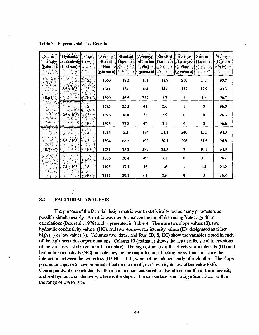
Table 3 Experimental Test Results.

Som ydal Slope Aeae Sadr;Aeae Sadd Avag Stdrd verg

Inte.sity ,nductivity (% Rnf .e. a. ...r . Deiti * eag D o CXls

~i'3 }, /0; ,rH ,f,5)va e. .t:

2 1360 18.5 151 11.9 208 56 95.7

6.5x iQ 5 1341 15.6 161 14.6 177 17.9 93.340 P

061 10 1390 46.5 347 8.3 1 1.6 967

2. 1693 25.5 41 2.6 0 0 96.5

i7.5x10 5 1696 10.0 35 2.9 0 0 96.3

1695 32.8 42 3.1 0 0 96.6

.2 1724 5.3 174 51.1 240 15.5 943

6.5x104. . $ 1804 66.2 193 50.1 206 31.5 94.8

0.77 i1o 1731 25.2 387 23.3 9 10.1 94.0

i ;: 2 2086 20.4 49 3.1 0 0.7 94.2

7.5x104 5 2105 17.4 46 1.6 1 1.2 94.9

10 2112 29.1 61 2.6 0 0 95.8

8.2 FACTORIAL ANALYSIS

The purpose of the factorial design matrix was to statistically test as many parameters as

possible simultaneously. A matrix was used to analyze the runoff data using Yates algorithm

calculations (Box et al., 1978) and is presented in Table 4. There are two slope values (S), two

hydraulic conductivity values (HC), and two storm-water intensity values (ID) designated as either

high (+) or low values (-). Columns two, three, and four (ID, S, HC) show the variables tested in each

of the eight scenarios or permutations. Column 10 (estimate) shows the actual effects and interactions

of the variables listed in column 11 (identity). The high estimates of the effects storm intensity (ID) and

hydraulic conductivity (HC) indicate they are the major factors affecting the system and, since the

interaction between the two is low (ID-HC = 1.0), were acting independently of each other. The slope

parameter appears to have minimal effect on the runoff, as shown by its low effect value (0.6).

Consequently, it is concluded that the main independent variables that affect runoff are storm intensity

and soil hydraulic conductivity, whereas the slope of the soil surface is not a significant factor within

the range of 2% to 10%.

49

Table 4 Experimental Yates Algorithm.

IntensityDrto (ID) 0.61 glnn(2.3 Vni)0.77 glm 2.

Hdulc6.5 i 10'sichsec', 7.5x14 inch/s4ec

Run VI'S G x.1 2 dvr esiae Idetit

I - - - 52.23 118.39 238.17 529.3 8 66.2 Avg

2 + - - 66.16 119.78 291.13 58.04 4 J

3 - + - 53.35 145.02 26.97 2.48 4 0.6 S

4 + + - 66.43 146.11 31.07 0.1 4 0 ID-S

5 - - + 64.97 13.89 1.39 52.96 4 jj jj c

6 + - 80.05 13.08 1.09 4.1 4 1 ID-HC

7 - + + 65.06 15.08 -0.81 -0.3 4 -0.1I S-HC

8 + + + 81.05 15.99 0.91 1.71 4 0.4 ID-S-HG

8.3 REGRESSION MODELING

Regression analysis serves as a basis for drawing inferences about relationships amongparameters in a system. Statistical models are built using procedures and conclusions drawn in aregression analysis depending on the assumption of a regression model. A model is perceived as themechanism that generates the data on which the regression analysis is conducted and is usually inalgebraic form. For example, if one assumes that the relationship is well represented by a linearstructure, a suitable model may be given by:

1l~iB 00BjX 1UB2X20B3X3[].... B~XU[

where:B0 l....= Regression Coefficients

U1 Model Error

50

Procedures in regression analysis involve drawing conclusions about regression coefficients.The [1 term is included to account for any model error and essentially describes the randomdisturbances. The above model is classified as linear and regression procedures involve fitting themodel to a set of data. The term, fitting, involves estimating the regression coefficients andcorresponding formulations of the fitted regression model, an empirical device that is the basis of anystatistical inference. Measure of the quality of fit is an important statistic that form the foundation ofanalyzing any regression model.

The experimental program tested a simulated landfill cover cell for moisture movement.Specifically, surface runoff from storm events. Slope, hydraulic conductivity, and storm intensity werechosen for the statistical evaluation based on water balance methods. The Yates algorithm (Table 4)analysis established storm intensity and hydraulic conductivity the main factors affecting predictivemodeling of the system. Multiple linear regression techniques were used in the model building process.The statistical analysis used 51 simulations, with the other 10 deemed as outliers. These 10 wereconsidered outliers because they did not achieve a mass balance of at least 90% or appeared to havesome experimental error. Errors associated with the simulations were as follows: runs 15,16,17 had afaulty collection container; run 58 had atmospheric rainfall enter into the closed system; and runs6,7,11,26,27,48 were low due to a loss of soil saturation (18, 30, and 9 days) between runs. Severalother runs (8,9,10,12,13,14) were deemed insufficient for the leakage and infiltration parametersbecause of intermingling of liquid in the collection containers. The system appeared to require severalruns after a prolonged drying period to achieve equilibrium in the soil matrix. The experimental datawas converted from a mass parameter to flux values, gallons per minute-acre, for a more descriptiveoutput. Regression summary outputs of the data are presented in Appendix VII.

8.3.1 Runoff

Modeling the runoff is the principal concern and uses storm intensity, slope, and hydraulicconductivity to predict runoff flux values. A linear structure is clearly seen from the experimental data.Table 5 shows the runoff regression models proposed. The correlation coefficients for the two runoffmodels are .983 and .984, respectively, indicating an excellent data fit. The slope parameter in therange tested, 2% to 10%, had little effect and may be deleted from the regression equation forsimplification. Residual plots of the three primary variables are presented in Figure 15. As parametervalues increase the residuals become increasingly spread indicating a funnel affect where, as theparameters are increased the system becomes more unstable. If the variance were greater, the datamay require transformation, but it appears insignificant over the range of variables tested in this study.The residual plots have a normal error response for the runoff model. Storm intensity (b) and hydraulicconductivity (a) clearly have a good linear fit as shown on Figure 16, but the slope (c) parameter hasno statistical significant impact. The hydraulic conductivity evaluation may be limited due to the 6.5 x10-5 inch/sec (1.6 x 104 cm/s) - 7.5 x I0F' inch/sec (1.9 x I0W cm/s) range of the variable (2 levels) inthe study. Although additional ranges of soil hydraulic conductivity were explored in the study, the soilmatrix was too impermeable to provide reliable data. The runoff model presented is an excellentestimator of runoff flux when the soil matrix is approximately at field capacity.

51

8.3.2 Other Parameters

Infiltration flux, leakage flux, and runoff+ infiltration flux parameters were also analyzed forpossible predictive characteristics. Table 5 presents these models and their correlation coefficients.The infiltration flux was examined using the same parameters as the runoff model and has a correlationcoefficient of 0.73, suggesting a less pronounced linear fit. The infiltration analysis consisted of 45experimental runs with six observations omitted due to insufficient infiltration observations. Twoleakage models are presented: a 3-variable model using 45 observed events and a second model using27 observed events. The second model uses only data from the first soil matrix where leakage wasreported. Data trends for the leakage models were difficult to predict due to the second soil profileproducing minimal leakage, which effectively gave only two parameters to evaluate. Residual plots ofthe 3-variable model are presented in Figure 17. Figure 18 conclusively shows a trend in the data that

indicates as the slope is increased the leakage flux decreased. The line fit plots for the slope clearlyindicate a linear fit with a correlation coefficient of 0.99 for the second model. The 3-variable model

shows a linear trend but is skewed by the second soil matrix producing minimal leakage as seen onFigure I8b. The leakage models have correlation coefficients of 0.76 (3-variable) and 0.91 (secondmodel). The leakage model may be enhanced by firther evaluation of soils with a larger range of

hydraulic conductivity then the range used in this study.

The models presented for the prediction of runoff flux has credibility based on the statisticalanalysis of the experimental results. The leakage model suggested a strong correlation exists between

slope and leakage; further evaluation is warranted. The proposed experimental models may becarefully used within the range of the variables tested.

52

Table 5 Regression Models.

Parameters R = Runoff Flux (gpm/acre)I = Infiltration Flux (gpmtacre)L = Leakage Flux (gpmtacre)HC = Hydraulic Conductivity (cm/sec)ID = Stormr Intensity (Iknin)S = Slope (%/*)W = Correlation CoefficientN = observations

Runoff Model(3-variables) R= -654.19(HC) + 738.94(1D) + 2.88(S)

R 0.984N=5195 % Confidence Interval = -697.99 < HC < -610.39

=727.59 <ID <750.29=-1.02<S<6.78

Runoff Model(2-variables) R = -653.4 I(HC) + 744.93(1D)

R2 0.983N=5195 % Confidence Interval = -697.71 < HC < -609.10

= 736.89 < ID< 752.97

Infiltration Model I = 318.33(HC) - 17.19(1D) - 13.29(S)(3-variables)

R2 =0.73N 4595 % Confidence Interval = 251.06 < HC < 385.60

= -33.95 < ID < -0.29=7.53<S <19.05

Leakage Model(3-variables) L = 308.48(HC) + 21.97(11D) - 14.14(S)

R2 = 0.76N=4595 % Confidence Interval = 249.31 < HC < 367.68

=7.16<ID<36.78=-19.21 < S < -9.08

Leakage Model(second model) L = 393.24(HC) + 21.97(1D) - 14.14(S)(one soil natrix)

R2 =0.91N=2795 % Confidence Interval= 175.09 < HC < 61139

--17.78 < ID < 77.72= -33.05 < S < -23.96

Runoff+ Infiltration Model R = -346.64(HC) + 719.86(ID) + 16.85(S)(3-variables)

R2 =0.96N=4595 % Confidence Interval = 413.94 < HC < -279.34

= 703.02 < ID < 736.70= 11.09<S<22.64

53

Residual Plot - Hydraulic Conductivity (HC)

100

50

1 -50 ' 0.1 0.2 0.3 0.4 0.5 10.6 070i 50

-100

Hydraulic Conductivity (cm/hr)

(a)

Residual Plot - Storm Intensity (ID)

100 -

X. 50 I

'U 0 it *$

-o 1.9 2.1 2.3 2.5 2.7 249 3 1

-100T

Storm Intensity (ID) (Ilmin)

(b)

I*

* 00

(c)

Figure 15 Residual Plots for Runoff Model (3-variables): (a) Hydraulic Conductivity, (b) StormIntensity, and (c) Slope.

54

Line Fit Plot - Hydraulic Conductivity (HC)

2500

Ez 1500

n T A Predicted Y2

5, 000- *~ 0 y- 384+968

pi CD 500 - Linear (Predicted Y) R =0.3868

0 0.1 0.2 0.3 0.4 0.5 0.6 0.7Hydraulic Conductivity (HC) (cmlhr)

(a)

Line Fit Plot - Storm Intensity (ID)2500 -

- 2000 y = 802.28x - 404.93 a2 10 2 =0.733 1

° Ad 10005A Predicted Y

- Linear (Predicted Y)0 I I I I

1.7 1.9 2.1 2.3 2.5 2.7 2.9 3.1

Storm Intensity (ID) (Imin)

(b)

Line Fit Plot - Slope (S)2500 -

~2000 -

ou 10001000 - - y=8.377x+ 1589.5

50 RH = 0.0058 A Predicted Y-Linear (Predicted Y)

0 V

0 2 4 6 8 10 12Slope (S) (%)

(c)

Figure 16 Line Fit Plots for Runoff Model (3-variables): (a) Hydraulic Conductivity, (b) StormIntensity, and (c) Slope.

55

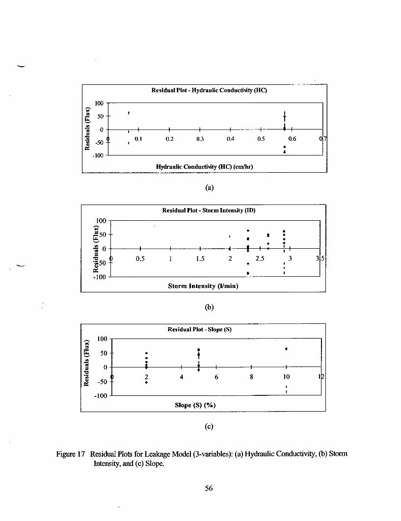
Residual Plot - Hydraulic Conductihity (HC)

100 *___dwa Pll-tyaii outiy(ll

0 I

-50 0.1 0.2 0.3 0.4 0.5 0.6 7

-100

Hydraulic Conductivity (HC) (cm/hr)

(a)

Residual Plot - Storm Intensity (ID)

100

p,50 , t

0 .0-II I 4 9. I ;I

0.5 1 1.5 2 2.5 3 3 5.a50

-100.

Storm Intensity (/min)

(b)

Residual Plot - Slope (S)

100 -

50 0

0~

2 4 6 8 10-50

-100~

Slope (5)(%

(c)

Figure 17 Residual Plots for Leakage Model (3-variables): (a) Hydraulic Conductivity, (b) StormIntensity, and (c) Slope.

56

Line Fit Plot - Slope (S) (3-variables)

y=-15.487x+ 17925 * Y

, 0R = 0.2745 * Predicted Y

20- Linear (Predicted Y

, 100-0 - I * I I

-100 2 4 6 8Slope (S) (%)

(a)

Line Fit Plot - Slope (S)

300 (only one hydraulic conductivity used)~.250k--

v 200 -- i Predicted Y150 -I - Linear (Predicted Y)

fA 100 + y=-28.449x+303.2250 R2 = 0.9901

0 I I I

0 2 4 6 8 10 12Slope (S) (%)

(b)

Figure 18 Line Fit Plots for Leakage Models: (a) Slope (3-variable) and (b) Slope (second model).

57

8.4 COMPARISON WITH HELP MODEL

The water balance methods (Section 3) are the basis for the HELP model analysis of landfillcover systems. Parameters used for the analysis must be properly estimated to balance the moisture ina landfill cover system. For these experimental simulations the evapotranspiration parameter isconsidered insignificant because of the short duration (30 minute) of the storm-event and the soilmoisture content was at approximate field capacity at the initiation of each simulation. Field capacitydefined by HELP is the soil moisture storage/content after a prolonged period of gravity drainage fromsaturation. Input values for the HELP modeling includes soil properties, hydraulic data, vegetativedata, meteorologic data, and initial conditions. Table 6 shows parameters for model simulationsincluding the experimental values and the default HELP model values used for the analysis. The HELPmodel default soils were chosen based on their saturated hydraulic conductivity and porosity valuesrather than their specific soil classification. Several HELP model output files, consistent with thevariables quantified in this study, have been included in Appendix V.

The storm events used in these studies cannot be directly integrated into the HELP model,since the HELP model parameters are based on 24 hour storm events. Consequently, the parametersfrom this study were manipulated in a manner to provide a format to integrate into the HELP model.For example, a simulated 30 minute-2.3 1pm storm event was converted to english units (inches) overthe cell area and then inserted in the HELP model as a 1 day storm event for comparison.

In order to model liner layers with the HELP model, one must classify the layer as a verticalpercolation, lateral drainage, barrier soil liner, or geomembrane liner. These classifications result in themodel using different parameters for the evaluation. Three liner scenarios were tested using the modeldefaults to detect the maximum runoff scenario and apply it to the comparison with the experimentalcell results. First, a simple 3-layer cover system with the soil layer divided into two parts (6" top soillayer and a 6" second soil layer for soil #1) and a bottom geomembrane liner was analyzed using threedifferent HELP model layer classifications. These HELP model classifications for the three scenarioswere (1) soil layers considered both vertical percolation layers, (2) soil layers considered both lateraldrainage layers, and (3) with a vertical percolation top layer with the second layer a lateral drainagelayer. The results indicate little difference in the simple 3-layer cover and how the soil layers areclassified for the simulations. Second, a more complex five layer cover liner system includinggeotextile and geonet was simulated and achieved no substantial difference than the previousscenarios. Subsequently, the experimental results were compared with the simple 3-layer system with avertical percolation layer, lateral drainage layer, and geomembrane liner layer as shown in Table 6.Results of all different layer combinations are presented in Appendix VI. The run numbers shown inTable 7 are associated with the Yates algorithm designations (see Table 4) for the experimentalsimulations. The HELP model estimates runoff lower than field results with the difference rangingfrom 8% to 24% for the eight simulated scenarios as shown in row 11 (F-D Error) on Table 7. Themodel underpredicted runoff for all the short-duration storm events simulated. These deductions areconsistent with the HELP model documentation that states the model is to be used for long termanalysis and may be deficient for short-term events (Schroeder et al., 1994).

58

Table 6 Parameters for Model Simulation.

Paaee aaeer- Exermeta Default HELP.Ma, ti Vaues VAlues

Soil Classification Liner I Soil SP # 10- ML(USC) Liner II Soil SP #15 -CH

Porosity Liner I Soil 0.372 0.398(volVol) Liner H Soil 0.371 0.475

Field Capacity Liner I Soil 0.244(vol/vol) Liner II Soil 0.265

Wilting Point Liner I Soil 0.136(volvol) Liner II Soil 0.265

Initial Soil Water Content Liner I Soil 0.290 0.290(vol/vol) Liner II Soil 0.236 0.265

Effective Saturated Liner I Soil 1.6 x 104 1.2 x 104

Hydraulic Conductivity Liner II Soil 1.9 x 10- 1.7 x 10-

(cm/s) Geomembrane 2.0 x 10-'3

Geomembrane Defects Installation Defects I(per acre) Pinhole Density 0 0

Evaporative Zone Liner I Soil 8Depth (inch) Liner II Soil 6

Leaf Area Index Liner I Soil 0 0Liner H Soil 0 0

Growing Season Liner I Soil 0-370(Julian day) Liner II Soil 0-370

SCS Surface Runoff Liner I 95-97Curve Number (CN) Liner II 95-97

Layer Thickness Liner I Soil 12 12(inch) Liner H Soil 10 10(mils) Geomembrane 60 60

Cover Slope Liner I 2,5,10 2,10(%) Linerll 2,5,10 2,10

Precipitation Liner I 1.99 1.99(inch) Liner II 2.51 2.51

Temperature Runs Tampa, Fl

Solar Radiation Runs Tampa, Fl

Evaporation Runs Tampa, Fl

59

Table 7 HELP Model Comparison with Experimental Results.

Runi Run2 Rin3 Ri;4 Ru 5 '' Run Rn7- Run 8

Str .9 25 .99 .5 199 21 1.9 .5

Experimentl unoff 1.51 1.91 1.54 1.94 1.88 2.31 1.88 2.34

() Rnff. 75.7 76.1 77.3 76.4 94.2 92.0 94.3 93.2

Deal uof 13 .9 1.35 1.42 1.39 1.91 1.4A19

() Runoff 67.3 55.4 67.8 56.6 69.9 76.1 70.4 77.7

Erwr 8.4 20.7 9.5 19.8 24.3 15.9 23.9 15.5

Run I - 11>0.61 gpm, S-20/o, HC-6.5 x IO-' in/sRun 2. -I=0.77 gpm, S-2r/o, HC=6.5 x 1O-1 WnSRun 3.- ID=0.61 gpmi, S=-10 0h., HC=6.5 x IO' in/sRun 4- D>0.77 gpm, S=10%,I-IC=6.5 x 10.' insRunm 5 D=0.61 gpm, S-=2%/, HC=7.5 x I 0r in/sRun 6. - D=0.77 gpm, S-20/o, H-C=7.5 x 0-6 insRun 7 -11>0.61 gpm, S5=10/., H-C=7.5 x 10O WsRun 8.11>D0.77 gpm, S5=10%/, HC=7.5 x 10.6 in/

60

9. CONCLUSIONS AND RECOMMENDATIONS

A laboratory scale model of a geomembrane liner final cover system was constructed to

simulate moisture movement through the system. The experimental program consisted of a mass

balance on the test cell for runoff, infiltration, and leakage parameters. Slope, hydraulic conductivity,

and storm intensity were chosen for a statistical evaluation based on the water balance methods.Multiple linear regression techniques were used to develop a runoff flux predicative model.

The results of this study serve to identify an approach to predicting surface runoff from

saturated landfill liner systems. Consequently, the design of surface runoff collection/storagerequirements can be more simply projected within the range of the variables evaluated in this study.

Generally, the saturation scenario for such predictions is encompassed in the experiments and resultant

regression models are presented herein. Further, the experimental results confirm previous evaluations

of the HELP models underprediction of surface runoff from landfills. It is also significant that the

experimental results demonstrated that at a slope of 10% the effects of leachate leakage through holes

in the underlying surface geomembrane liner are minimized. Obviously, such a slope mitigates thecreation of sufficient static head in the soil above the liner to facilitate infiltration through the

geomembrane liner. These results may also be translated into the effects of slope on the bottom liner

leakage rates in landfills (i.e., a slope of 10% on the bottom liner may inhibit leakage in the bottom liner

system).

Limitations of the HELP model may be associated with the SCS curve number methods used.

The SCS curve numbers were derived from case studies of ungauged watersheds that may not be

applicable to landfill applications and be used beyond their respective scope for application to landfill

surfaces. The SCS curve number is a sensitive parameter which must be accurately estimated to obtain

good results for model prediction. The experimental regression models indicate a better estimator of

runoff during larger storm events. The SCS methods may also suffer from the omission of a time

increment. The time increment may have a major impact in the runoff produced. Default curve

numbers supplied by the HELP model tend to underpredict runoff.

Follow-up research should be performed using other ranges of the parameters selected for this

study. Additional soil matrices with a broader range of hydraulic conductivity may enhance the leakage

model. The regression models need to be analyzed to determine whether a single or a series ofregression equations should be developed specifically designed for landfill use. Further, based on the

literature review, capillary barriers need to be evaluated for the impediment of infiltration. Also, the use

of geotextile material to separate soil materials in capillary barriers needs to be investigated to estimate

effects this may have on capillary suction. Reduction of leakage with these systems may be possible,

but current experimental field data is not sufficient to substantiate this matter.

61

10. REFERENCES

Action Leakage Rates for Leak Detection Systems, EPA-530-R-92-004, U.S. EnvironmentalProtection Agency, Office of Solid Waste, 1992.

Z.Y. Al-Jobeh, Finite Element Model of Overburden Induced Flow in Unsaturated Hydraulic Barrers,Dissertation, The University of Toledo, 1994.

A.E. Arnold, Experimental and Mathematical Modeling of Moisture Transport in Landfills, M.S.Thesis, Tufts University, 1989.

G. Aron, "Adaptation of Horton and SCS Infiltration Equations to Complex Storms," Journal ofIrrigation and Drainage Division Engineering 118 (2): 275 (1992).

A. Bagchi, Design. Construction and Monitoring of Sanitary Landfills, John Wiley & Sons, Inc., NewYork, 1990.

B.J. Barfield, RC Warner and C.T. Haan, Applied Hydrology and Sedimentology for DistributedAreas, Oklahoma Technical Press, Stillwater, 1981.

F.J. Barnes and J.C. Rodgers, Project Summary: Evaluation of Hydrologic Models in the Design ofStable Landfill Covers, EPA/600/S2-88-048, U.S. Environmental Protection Agency, Research andDevelopment, 1988.

J.M. Bass, W.J. Lyman, J.P. Tratnyek and A.D. Little, Assessment of Synthetic Membrane Successesand Failures at Waste Storage and Disposal Sites, EPA/600/2-85-100, U.S. Environmental ProtectionAgency, Office of Research and Development, Cincinnati, 1985.

P.B. Bedient and W.C. Huber, Hydrology and Floodplain Analysis, Addison-Wesley PublishingCompany, Massachusetts, 1988, pp 101-107.

C.H. Bensen and R.J. Pliska, "Final Covers: HELP Needs Help From the Field," Waste Age 89(March 1996).

R.L. Bingner, C.K. Mutchler and C.E. Murphree, "Predictive Capabilities of Erosion Models forDifferent Storm Sizes," Transactions of American Society of Agricultural Engineers 35 (2): 505(1992).

S.C. Boggs, Multi-Axil Geomembrane Seam Testing, M.S.C.E. Thesis, University of South Florida,Tampa, 1995.

R. Bonaparte, J.P. Giroud and B.A. Gross, "Rates of Leakage Through Landfill Liners," inProceedings of 1989 Geosynthetic Conference, 1989, pp 18-29.

62

R. Bonaparte and B.A. Gross, "Field Behavior of Double-Liner Systems," Waste ContarninantSystems: Construction. Regulation. and Performance, Geotechnical Special Publication No. 26, ASCE,1990, pp 52-83.

K.W. Brown, J.C. Thomas, R.L. Lytton, P. Jayawickrama, and S.C. Bahrt, Project Summ=ary-Quantification of Leak Rates Through Holes in Landfill Liners, EPA/600/S2-87-062, U.S.Environmental Protection Agency, Hazardous Waste Research Laboratory, Cincinnati, 1987.

G.E.P. Box, W.G. Hunter, and J.S. Hunter, Statistics for Experimenters, John Wiley & Sons, NewYork, 1978, p 302.

S.E. Buss, A.P. Butler, P.M. Johnston, C.J. Sollars and R. Perry, "Mechanisms of Leachate throughSynthetic Landfill Liner Materials," J.CIWEM 353 (1995).

P.E. Clopper, Antecedent Moisture Consideration in the SCS Curve Number Rainfall-Runoff Model,M.S. Thesis, Colorado State University, Fort Collins, 1980.

A.L. Coates, Hydrologic Performance of Multilayer Landfill Covers: A Field Verification andModeling Assessment of HELP and SOILINER, M.S. Thesis, University of Kentucky, 1987.

D.E. Daniel, "Soil Barrier Layers Versus Geosynthetic Barriers in Landfill Cover Systems,"Geotechnical Special Publication, ASCE, (53): 1 (1995).

D.E. Daniel, "Surface Barriers: Problems, Solutions, and Future Needs," In-Situ Remediation:Scientific Basis for Current and Future Technologies, G.W. Gee and N.R. Wing, Eds.: Battelle Press,Columbus, 1994, pp 441487.

D.E. Daniel, C.D. Shackelford, W.D. Liao and H.M. Liljestrand, Rate of Flow of Leachate ThroughClay Soil Liners, EPA/600/2-91/021, U.S. Environmental Protection Agency, Risk ReductionEngineering Laboratory, Cincinnati, 1991.

E. Dass, G.R. Tarnke and C.M. Stoffel, "Leachate Production at Sanitary Landfill Sites," Journal of theEnvironmental Engineering Division, ASCE, 107 (EE6): 49 (1977).

A.C. Demetracopoulos, "Overview of Bottom Liners," Water Resource Bulletin 24 (1): 49 (1988).

A.C. Demetracopoulos, G.P. Korfiatis, E.L. Bourodimos, and E.G. Naway, "Modeling for Design ofLandfill Bottom Liners," Journal of Environmental Engineering, ASCE, 110 (6): 1084 (1984).

A.C. Demetracopoulos, G.P. Korfiatis, E.L. Bourodimos and E.G. Naway, "Unsaturated FlowThrough Solid Waster Landfills: Model and Sensitivity Analysis," Water Resource Bulletin 22 (4): 601(1986).

M. Devaurs and E. Springer, "Representing Soil Moisture in Experimental Trench Cover Designs forWaste Burial with the Creams Model," Hazardous Waste and Hazardous Materials 5 (4): 295 (1988).

63

Design and Construction of RCRA/CERCLA Final Cover, EPA/625/4-91/025, U.S. EnvironmentalProtection Agency, Office of Research and Development, Washington D.C., 1991, p 4.

T.S. Dozier, Examination and Modification of Three Surface-Hydrology Processes in the HELP(Hydrologic Evaluation of Landfill Performance) Model, Dissertation, Mississippi State University,1992.

M. El-Fadel, A.N. Findikakis and J.O. Leckie, "Modeling Leachate Generation and Transport in SolidWaste Landfills," Environmental Technology 18: 669 (1997).

Y. Faure, "Design of Drain Beneath Geomembranes: Discharge Estimation and Flow Patterns in theCase of Leak," in Proceedings of International Conference on Geomembranes," Vol. 2, IndustrialFabrics Association International, Denver, 1984, pp 463-468.

MJ. Fayer and T.L. Jones, UNSAT-H Version 2.0: Unsaturated soil Water and Heat Flow Model,PNL-68 10, Pacific Northwest Laboratories, Richland, 1990.

M.J. Fayer, M.L. Rockhold, and M.D. Campbell, "Hydrologic Modeling of Protective Barriers:Comparison of Field Data and Simulation Results," Soil Science Society American Journal 56: 690(1992).

D.G. Fenn, K.J. Hanley and T.V. DeGeare, Use of The Water Balance Method for Predicting leachateGeneration From Solid Waste Disposal Sites, Report ( SW-168), U.S. Environmental ProtectionAgency, Office of Solid Waste Management, 1975.

W.E. Fleenor and I.P. King, "Defining Limitations for Use of the HELP Model," in Proceedings ofthSixth Annual International Conference, ASCE, Las Vegas, 1995a, pp 185-187.

W.E. Fleenor and I.P. King, "Identifying Limitations on Use of the HELP Model," GeotechnicalSpecial Publication No. 23, ASCE, New York, 1995b, pp 121-138.

M. Fukuoka, "Large Scale Permeability Test for Geomembranes Subgrade System," in Proceedings ofThird International Conference on Geomembranes," Vol.3, Vienna, 1986, pp 917-922.

J.R. Gee, "Prediction of Leachate Accumulation in Sanitary Landfills," in Proceedings of FourthAnnual Madison Conference of Applied Research and Practice on Municipal and Industrial Waste.1981, pp 170-190.

L.W. Gelhar, "Stochastic Subsurface Hydrogeology from Theory to Application," Water ResourcesResrh 22 (9): 1355 (1986).

R.B. Gilbert, Performance Reliability of Landfill Lining Systerns, Dissertation, University of Illinois atUrbana-Champaign, 1993, p 6.

64

J.P. Giroud, "Impermeability: The Myth and a Rational Approach," in Proceedings of InternationalConference on Geomembranes. Vol. I, IFAI, Denver, 1984, pp 157-162.

J.P Giroud, K. Badu-Tweneboah and R. Bonaparte, "Rate of Leakage Through a Composite Liner

Due to Geomembrane Defects," Geotextiles and Geomembranes 11: 1 (1992).

J.P Giroud and R Bonaparte, "Leakage Through Liners Constructed with Geomembranes - Part I.

Geomembrane Liners," Geotextiles and Geomembranes 8 (1): 27 (1989a).

J.P. Giroud and R. Bonaparte, "Leakage Through Liners Constructed with Geomembranes - Part II.Composite Liners," Geotextiles and Geomembranes 8 (2): 71 (1989b).

J.P. Giroud and J.E. Fluet; Jr., "Quality Assurance of Geomembranes," Geotextiles andGeomembranes 3: 249 (1986).

J.P. Giroud and R.K. Frobel, Geomembrane Products, Geotechnical Fabrics Report, 1983, pp 3842.

J. P. Giroud, A. Khatami and K. Badu-Tweneboah, "Evaluation of the Rate of Leakage ThroughComposite Liners," Geotextile and Geomembranes 8: 337 (1989).

R.H. Hawkins, "Improved Prediction of Storm Runoff in Mountain Watersheds," Journal of Irrigation

and Drainage Division, ASCE, 99 (IR4): 519 (1973).

R.H. Hawkins, "Discussion of Aron an Others," Journal of Irrigation and Drainage Division, ASCE,104 (IR4): 464 (1979).

T.M. Holsen, J.K. Park, D. Jenkins and R.E. Selleck, "Contamination of Potable Water by Permeationof Plastic Pipe," Journal of American Water Works Association 83 (8): 53 (1991).

P.W. Jayawickrama, K.W. Brown, J.C. Thomas and RL. Lytton, "Leakage Rates through Flaws inMembrane Liners," Journal of Environmental Engineering, ASCE, 114 (6): 1401 (1988).

RM. Khanbilvardi, R.M., S. Ahmed, and P.J. Gleason, "Flow Investigation for Landfill Leachate(FILL)," Journal of Environmental Engineering, ASCE, 121 (1): 45 (1995).

R-M. Khanbilvardi, S. Ahmed and P.J. Gleason, "Prediction of Runoff-Evapotranspiration to estimateleachate generation in a Landfill," Water Resource Planning and Management and Urban Water

Resources, ASCE, 37 (1991).

W.G. Knisel and A.D. Nicks, CREAMS - A Field Scale Model for Chemical. Runoff. and Erosionfrom Agricultural Management System, Conservation Research Report Number 26 U.S. Departmentof Agriculture, 1980.

R.M. Koerner, Designing with Geosynthetics, 3rd ed., Prentice Hall, Englewood Cliffs, 1994.

65

G.P. Korfiatis, Modeling the Moisture Transport Through Solid Waste Landfills, Dissertation, Rutgers

University, 1984.

G.P. Korfiatis and A.C. Demetracopoulos, "Flow Characteristics of Landfill Leachate CollectionSystems and Liners," Journal of Environmental Engineering, ASCE, 112 (3): 538 (1986).

M.D. LaGrega, P.L. Buckingham and J.L. Evans, Hazardous Waste Management, McGraw-Hill, Inc.,

New York, 1994, pp 803-807.

D. Laine, "Analysis of Pinhole Seam Leaks Located in Geomembrane Liners Using the Electrical Leak

Location Method: Case Histories," in Geosynthetics Conference, Atlanta, 1991, pp 239-253.

J. Lee, Performance of Landfill Cover Systems in Cold Climates, Dissertation, Wayne State University,

1994, p 27.

B.M. McEnroe, "Drainage of Landfill Covers and Bottom Liners: Unsteady Case," Jounal of

Environmental Engineering, ASCE, 115 (6): 1103 (1989a).

B.M. McEnroe, "Maximum Saturated Depth Over Landfill Liner," Journal of Environmental

Engineering, ASCE, 119 (2): 262 (1993).

B.M. McEnroe, "Steady Drainage of Landfill Covers and Bottom Liners," Journal of Environmental

Engineerng, ASCE, 115 (6): 1114 (1989b).

B.M. McEnroe and P.R Schroeder, "Leachate Collection in Landfills: Steady Case," Journal of

Environmental Engineering, ASCE, 114 (5): 1052 (1988).

M.J. Mack "HER - Hydrologic Evaluation of Runoff: the Soil Conservation Service Curve Number

Technique as an Interactive Computer Model," Computers and Geosciences 21 (8): 929 (1995).

M.J. Mack, MILL (Computer) Model Investigation of Landfill Leachate, Dissertation, University of

Delaware, 1991.

C.D. Martin, Critique of the SCS Runoff Model, M.S. Thesis, The Pennsylvania State University,

University Park, 1979.

S. Melchior, K Berger, B. Vielhaber and G. Miehich, "Multilayer Landfill Covers: Field Data on theWater Balance and Liner Performance," In-Situ Remediation: Scientific Basis for Current and Future

Technologies, G.W. Gee and N.R. Wing, Eds.: Battelle Press, Columbus, 1994, pp 4 1 1425.

RJ. Montgomery, A Data-Based Evaluation of the SCS Cover Number Method for Runoff

Predictions, M.S. Thesis, Colorado State University, Fort Collins, 1980, pp 16-22.

Municipal Solid Waste Landfill Alternative Design Closure Guidance, Final Guidance, Florida

Department of Environmental Protection, Tallahassee, 1995, pp 3-6.

66

R.J. Murphy and S. A. Batiste, Drainage Media for Distribution of Recycled leachate, Interim FinalReport - Volume III, for State University System of Florida, Center for Solid and Hazardous Waste

Management, Gainesville, 1991, pp 1-2.

R.J. Murphy and J.A. Borgmeyer, Evaluation of Leakage Rates in a Geomembrane Double Liner

Sys , Final Report, for A.R.M. Saleh of Camp Dresser & McKee, Inc. and S. Ortolon of GundleLining Systems, Inc., 1993, pp 2-4.

National Engineering Handbook, Section 4 - Hydrology, SCS/ENG/NEH-4-2, U.S. ConservationService, U.S. Government Printing Office, 1972.

W.B. Nixon, A Risk Mitigation Methodology for Solid Waste Landfills, Dissertation, University of

South Florida, Tampa, 1995, pp 21-22.

W.B. Nixon and R.J. Murphy, "Environmental Hazardous Assessment Models: An Overview," in

Proceedings of the 88' Annual Meeting of the A&WMA, 95-RD-144.01, Air & Waste Management

Association, San Antonio, 1995.

J.J. Noble and A.E. Arnold, "Experimental and Mathematical Modeling of Moisture Transport in

Landfills," Chemical Engineering Communication 100: 95 (1991).

J.W. Nyhan, "Calibration of the CREAMS Model for Landfill Cover Designs Limiting Infiltration of

Precipitation at Waste Sites," Hazardous Waste and Hazardous Materials 7 (2): 169 (1990).

J.W. Nyhan, Hydrologic Modeling to Predict Performance of Shallow Land Burial Cover DesignsatLos Alamos National Laboratory, LA-i 1533-MS, Los Alamos National Laboratory, 1989.

G. Ostroff, "Flow Investigation For Landfill Leachate (FILL)," Journal of Environmental EngineeringASCE, 122 (1): 86 (1996).

J.K. Park and M. Nibras, "Mass Flux of Organic Chemical Theory Polyethylene Geomembranes,"

Water and Environmental Resources 65: 227 (1993).

E.R. Perrier and A.C. Gibson, Hydrologic Simulation on Solid Waste Disposal Sites (HSSWDS), SW-

868, U.S. Environmental Protection Agency, Municipal Environmental Research Laboratory,Cincinnati, Ohio, 1980.

N. Peters, Construction, Instrumentation Monitoring and Modeling of Multi-Layer Soil Landfill

CoQy[, Dissertation, University of Kentucky, 1992, p 1.

R.L. Peyton and P.R. Schroeder, "Evaluation of Landfill-Liner Designs," Journal of Environmental

Enginering, ASCE, 116 (3): 421 (1990).

R.L. Peyton and P.R. Schroeder, "Field Verification of HELP Model for Landfills, "Journal of

Environmental Engineering, ASCE, 114 (2): 247 (1988).

67

J.R. Philip, "Theory of Infiltration," Advances in Hydroscience: V.T. Chow, Ed., Academic Press,New York, 1969, pp 215-296.

J.T. Richie, "A Model for Predicting Evaporation from a Row Crop with Incomplete Cover," WaterResources Research 8 (5): 1204 (1972).

P.R Schroeder, T.S. Dozier, P.A. Zappi, B.M. McEnroe, J.W. Sjostrom, and RL. Peyton, OkMHydrologic Evaluation of Landfill Performance (HELP) Model: Engineering Documentation forVersion 3, EPA/600/R-94/168b, U.S. Environmental Protection Agency, Risk Reduction EngineeringLaboratory, Cincinnati, 1994.

P.R Schroeder, A.C. Gibson and M.D. Smolen, The Hydrologic Evaluation of Landfill Performance(HELP) Model - Volume H. Documentation for Version 1, EPA/530-SW-84-009, U.S.Environmental Protection Agency, U.S. Army Engineer Waterways Experimental Station, Vicksburg,1984b.

P.R Schroeder, J.M. Morgan, T.M. Walski and A.C. Gibson, Hydrologic Evaluation of LandfillPerformance (HELP) Model: Volume I. User's Guide for Version 1. Draft Report. EPA/530-SW-84-009, U.S. Environmental Protection Agency, Municipal Environmental Research Laboratory,Cincinnati, Ohio, 1984a.

P.R. Schroeder and R.L. Peyton, Verification of Lateral Drainage Component of the HELP ModelUsing Physical Models, EPA/600/S2-87/049, U.S. Environmental Protection Agency, HazardousWaste Engineering Research Laboratory, Cincinnati, 1988a.

P.R. Schroeder and RL. Peyton, Verification of the Hydrologic Evaluation of Landfill Performance(HELP) Model Using Field Data, EPA/600/S2-87/050, U.S. Environmental Protection Agency,Hazardous Waste Engineering Research Laboratory, Cincinnati, 1988b.

R.W. Skaggs, A Water Management Model for Artificially Drained Soils, Technical Bulletin Number267. North Carolina Research Services, 1980.

Soil Conservation Service, National Engineering Handbook, Section 4 - Hydrology, SCS/ENG/NEH-4-2, U.S. Government Printing Office, Washington D.C, 1985.

SOILINER Model - Documentation and User's Guide (Version 1), EPA/530-SW-86-006a, U.S.Environmental Protection Agency, Hazardous Waste Research Laboratory, Cincinnati, 1986.

Solid Waste Disposal Facility Criteria. Technical Manual, EPA-530-R-93017, U.S. EnvironmentalProtection Agency, Office of Solid Waste and Emergency Response, Washington D.C., 1993, pp pfl-pf2l.

RI. Stessel and P. Goldsmith, "Flexible Membrane Liner Testing in Waste Management," Journalfthe Air & Waste Management Association 42: 1178 (1992).

68

W.A. Straub and D.R. Lynch, "Models of Landfill Leaching: Moisture Flow and Inorganic Strength,"Journal of Environmental Engineering, ASCE, 108 ( EE2): 231 (1982).

R-A. Sudar, KE. Saxon and R.G. Spomer, "A Predictive Model of Water Stress in Corn andSoybean," Transactions of American Society of Agricultural Engineers, 97 (1981).

G. Tchobanoglous, H. Theisen and S. Vigil, Integrated Solid Waste management EngineeringPrincipals and Management Issues, McGraw-Hill, Inc., New York, 1993, pp 361, 452-455, 24-33.

Technical Manual for Solid Waste Disposal Facility Criteria - 40 CFR Part 258, U.S. EnvironmentalProtection Agency, 1992, pp F2-F 19.

R.B. Tedder, Memorandum-Landfill Liner Cost Benefit Analysis, Florida Department ofEnvironmental Regulation, September 8, 1992.

F.L. Thompson and S.W. Tyler, Comparison of Two Groundwater Flow Models - UNSATID andHELP, CS-3695, Electric Power Research Institute, Battelle, Pacific Northwest Laboratories, PaloAlto, 1984.

C.W. Thomthwaite, "Average Climatic Water Balance data of the continents," Climatology 17 (3):419 (1964).

C.W. Thornthwaite and J.R. Mather, "Instruction and Tables for Computing PotentialEvapotranspiration and the Water Balance," Climatology 10 (3): 185 (1957).

C.W. Thornthwaite and J.R. Mather, "The Water Balance," Climatology 8 (1): 104 (1955).

Unsaturated Groundwater Flow Model (UNSATID) Computer Code Manual, CS-2434-CCM,Electric Power Research Institute, Pacific Northwest Laboratories, Palo Alto, 1981.

R.B. Wallace and H. Akgun, "Leakage Through Liners: A Practical Approach to Design," inProceedings of the 44th Canadian Geotechnical Conference, Vol. 2 No. 78, Canadian TechnicalSociety, 1991.

J.C. Walton and B. Sagar, "Aspect of Fluid Flow through Small Flaws in Membrane Liners,"Environmental Science and Technology 24 (6): 920 (1990).

M.P. Wanielista and A. Yousef, Stormwater Management, John Wiley & Sons, Inc., New York, 1993,pp 70-76.

R.C. Warner, N. Peters, A.C. Coates, D.S. Logsdon, Y.H. Huang and D. Greer, Design. Construction.Instrumentation. Monitoring. and HELP Model Evaluation of Multiple-Layer Soil Covers,Cooperative Agreement CR-810431-01, U.S. Environmental Protection Agency, Hazardous WasteResearch Laboratory, Cincinnati, 1989.

69

J.R. Williams and W.V. LaSeur, "Water Yield Model Using SCS Curve Numbers," Journal of theHydraulics Division, ASCE, 102 (HY.): 1241 (1976).

M.R. Woyshner and E.K. Yanful, "Modeling and Field Measurements of Water Peculation Throughand Experimental Soil Cover on Mine Tailings," Canadian Geotechnical Journal 32: 601 (1995).

T.H. Wu, J.A. Hall and J.V. Bonta, "Evaluation of Runoff and Erosion Models," Journal of Irrigationand Drainage Engineering, ASCE, 119 (4): 364 (1993).

C. Ziess and W. Major, "Moisture Flow Through Municipal Solid Waste: Patterns andCharacteristics," Journal of Environmental Systems 22 (3): 211(1992-93).

70

APPENDICES

71

APPENDIX 1. COEFFICIENT OF PERMEABILITY

COEFFICIENT OF PERMEABILITY -Constant Head Method (ASTM D2334

Soil SampleDescription of SoilDate of TestingSample DiameterSample Area (A)Sample Height (L)Sample VolumeWeight of SampleConstant Head Height (h)

ISP - Poorly Graded Sand5/15/977.62c45.6 cm214.3m652.1m1157.2 grams50.2m

Test Number' t scds Q, cm3 TenperatureC

I 1800 54 23

2 1800 53 24

3 1800 49 24

Average 1800 52 24

K71 QL/Aht =(52X14.3)/ 45.6)(50.2)(1800)= 1.8 x I0 4cm/s

[], 20u 2O -iK20[1K707 L 20 = 1.64x 104 cm/s

Soil Sample 2Description of Soil SP - Poorly Graded SandDate of Testing 6/26/97Sample Diameter 7.62 cmSample Area (A) 45.6 cm2

Sample Height (L) 14.3 cmSample Volume 652.1cm3

Weight of Sample 1178.2 gramsConstant Head Height (h) 90.2 cm

Test Number: t,seconds Q, cm3 Temperature, C

1 1800 10.4 22.5

2 1800 10.4 22.5

3 1800 10.4 22.5

Average 1800 10.4 22.5

K7EIQLIAht = (10.4X14.3)/(45.6X90.2)(1800) = 2.0 x lIW cm/s

7 TI20= 0953K20E1K70E1 7A 20= 1.9x 105 cm/s

72

APPENDIX II. GRAIN SIZE DISTRIBUTION

GRAIN SIZE DISTRIB3UTION-MECHANICALSample Preparation - ASTM D421Soil Sample Size - ASTM D1 140-54Test Soil # 1Weipht of anmnle. Ws = '5O e

5/9/97 5113197 Ave_ gSiev , Dianmte Weigb' Weight Weight % %

Number (mm) 'Retaied Retaind. Retained Retained Passing

._ _ ' ) (O .) (8) '_ _ '._ _._,_)'

4 4.75 2.0 2.1 2.1 0.4 99.6

10 2.00 3.2 4.8 4.0 0.8 98.8

20 0.850 5.9 6.1 6.0 1.2 97.6

40 0.425 10.0 112 10.6 2.1 95.5

60 0.250 37.1 57 47.1 9.4 86.1

140 0.106 396.4 379.6 388.0 77.6 8.5

200 0.075 35.7 29.7 32.7 6.5 2.0

8.4 7.8 8.1 1.6

Unified Soil Classification SystemSoil Classification: SP Poorly Graded Sand

Cu = D60/D10 = .20/.10 = 2.0Cc = (D30)2/DIO*D60 = (.140)2/.20*.10 = 0.98

Test Soil # 2Weight of Sample, Ws=500 e_ _

6/26/97 6/26/97 Av-VeSieve Diamder Weight Wei Weig % h

Nwmber (mm) Retained Retained Retained Retained, Passing

._ _. (8) (18) (a) ._ _ _ _

4 4.75 0.4 0 02 0.04 99.9

10 2.00 3.5 1.5 2.5 0.5 99.5

20 0.850 7.5 4.6 6.1 1.2 98.3

40 0.425 15.9 13.4 14.7 2.9 95.4

60 0.250 54.1 645 59.3 11.9 83.5

140 0.106 400.6 384.3 392.5 78.5 5.0

200 0.075 3.3 13.2 8.3 1.7 3.3

14.1 17.3 15.7 3.1

Unified Soil Classification SystermSoil Classification: SP Poorly Graded Sand

Cu=D60/D10=.20/.10= 1.75Cc = (D30)2/D1O*D60 = (.140f/.20*.10 = 0.89

73

APPENDIX HI. WATER-CONTENT DETERMINATION

Water-Content DeterminationASTM D2216

Soil I 1

Dish Wet Dish + Sample Dry Dish Fi- Sample WaterDry(grams) Sample Wet S pe D.y Content

Dish I (grams),@ ms) i (grams) (grams) (%)

1 90.895 304.0 213.1 265.5 174.6 18.1

2 89.089 265.7 175.9 234.7 144.9 17.6

3 92.912 249.9 156.9 225.1 132.2 15.7

Avg 17.1

Soil #2,

Dish Wet Dish + Sample Dry Dish + Sample Water(grams) Sample Wet Sample Dry Content

Dish . _._,,_. (gams) (grams) (grams) (rM ) ()

1 90.895 272.2 181.3 247.2 156.3 13.8

2 89.809 270.2 180.4 245.2 155.4 13.9

3 92.912 267.8 174.9 243.1 150.2 14.1

Avg 13.9

Moisture content samples taken 4 hours after cell at saturation

Samples taken 2', 4', and 6' fiom the outlet on center at a 6" depth

MOISTURECONTEN7n0 0-I 100WI

74

APPENDIX IV. EXPERIMENTAL RUNS

Date Rm Sod Hydraulic Stwm Storn Total Sbpe Rmnoff hnihraton Leakage# lassification Conitcity hneitr Yea Rainfal t%) (kg) (kg) (kg)

(USC) (cisec) (k) (kg)

2/27/97 I SP 1.6 x H0O 2.30 2 69.00 5 50.84 5.88 6.42

2/27197 2 SP 1.6x 104 2.30 2 69.00 5 51.46 6.30 7.60

2/27/97 3 SP 1.6x I0O' 2.30 2 69.00 5 52.36 6.46 7.44

3/5/97 4 SP 1.6 x 104 2.64 5 79.20 5 60.04 6.98 6.86

3/6/97 5 SP 1.6x I04 2.64 5 79.20 5 61.36 5.38 6.20

3124197 6 SP 1.6 x 10'4 2.64 5 79.20 5 56.88 2.62 0

3/25/97 7 SP 1.6x l0' 2.64 5 79.20 5 64.99 7.40 1.70

3/26/97 8 SP 1.6x I0-4 2.90 10 87.00 5 71.02 8.74 1.58

3/26197 9 SP 1.6x I0W 2.90 10 87.00 5 70.72 9.76 2.28

3127197 10 SP 1.6x lO 2.90 10 87.00 5 71.56 9.30 1.70

511197 1I SP 1.6x 10 * 2.09 - 62.70 5 43.66 10.06 0.84

5/1/97 12 SP 1.6x 10-4 2.09 62.70 5 44.82 10.56 3.36

5/2/97 13 SP 1.6x 10 2.09 62.70 5 45.74 9.42 3.48

5/2/97 14 SP 1.6x 104 2.09 62.70 5 45.00 9.06

5/5/97 15 SP 1.6 x 104 3.10 93.00 5 67.82 6.08 u.o4

5/5/97 16 SP 1.6x 1o04 3.10 - 93.00 5 72.10 10.58 0.80

5/6197 17 SP 1.6x 10-4 2.30 2 69.00 5 52.14 0.62 6.12

516197 18 SP 1.6x 104 2.30 2 69.00 5 51.04 6.82 6.16

517197 19 SP 1.6x 10-4 2.30 2 69.00 5 51.60 5.36 6.26

5f7197 20 SP 1.6x 10' 2.64 5 79.20 5 61.34 6.04 8.12

X - Data not used

75

APPENDIX IV. CONTINUED

Date Run So Hydraulic Stm Strmn TotW Slope Runoff Infitatkon L-akage# Cksficaion Condidvity InMensty Yea Rainfall /0) (kg) (kg) (kg)

:Usc_ (cnmsec) (hnin) (kg)

5m197 21 SP 1.6x IO4 2.64 5 79.20 5 61.34 6.50 8.00

5m197 22 SP 1.6 x 104 2.90 10 87.00 5 66.34 6.76 8.54

5/8/97 23 SP 1.6 x 104 2.90 10 87.00 5 69.20 5.88 8.68

5/8/97 24 SP 1_6x Io0 1.99 - 59.70 5 42.58 6.40 7.82

54/97 25 SP 1.6x 104 1.99 - 59.70 5 41.34 6.38 7.86

5/17/97 26 SP 1.6x 10' 2.30 2 69.00 2 50.12 9.14 2.56

5/17/97 27 SP 1.6 x 10' 2.30 2 69.00 2 52.58 3.90 9.06

5/17/97 28 SP 1.6 x l0r 2.30 2 69.00 2 51.40 5.26 8.22

5/17/97 29 SP 1.6x I0W 2.30 2 69.00 2 52.56 6.12 7.96

5/18/97 30 SP 1.6x 104 2.30 2 69.00 2 52.66 5.98 7.80

5/18/97 31 SP 1.6x IO4 2.90 10 87.00 2 66.24 7.84 9.16

5/19/97 32 SP 1.6x I0 2.90 10 87.00 2 66.30 4.40 9.82

5/19/97 33 SP 1.6 x IOr' 2.90 10 87.00 2 65.94 7.80 8.64

5/19/97 34 SP 1.6x 10' 4 2.90 10 87.00 5 65.60 9.56 6.54

5120/97 35 SP 1.6 x 10- 1.99 - 59.70 5 42.86 7.20 6.12

5120/97 36 SP 1.6 x 104' 2.30 2 69.00 10 51.88 13.42 0

5/20/97 37 SP 1.6x IO- 2.30 2 69.00 10 52.84 13.58 0.10

5121/97 38 SP 1.6 x 10' 2.30 2 69.00 10 55.34 . 12.98 0.04

5121/97 39 SP 1.6 x I0O 2.90 2 69.00 1O 65.56 15.84 0.80

5122/97 40 SP 1.6x 104 2.90 10 87.00 10 67.44 14.18 0.14

X - data no( used

76

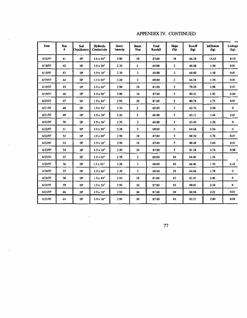
APPENDIX IV. CONTINUED

Date RunSoti-

ilydmulic summSftnitySumYear

TOalR~nafl

Runoff(kg)

nfautmxim(Wg

Leakage(kg)

5122/97 41 SP 1.6x 10' 2.90 10 87.00 10 66.28 15.62 0.10

6/18/97 42 SP 1.9 x l0-' 2.30 2 69.00 2 66.08 1.50 0.01

6/18/97 43 SP 1.9 x 10' 2.30 2 69.00 2 64.60 1.58 0.01

6/19/97 44 SP 1.9 x 107 2.30 2 69.00 2 64.24 1.70 0.01

6/19/97 45 SP 1.9x IO C 2.90 10 87.00 2 79.20 1.98 0.01

6/19/97 46 SP 1.9 x I0O5 2.90 10 87.00 2 80.22 1.92 0.04

6/20/97 47 SP 1.9x io0 ' 2.90 10 87.00 2 80.74 1.75 0.01

6/21/97 48 SP 1.9x I0o 2.30 2 69.00 5 62.76 2.50 0

6/21/97 49 SP I.9x 10 2.30 2 69.00 5 65.12 1.44 0.01

6/22/97 50 SP 1.9x 10 2.30 2 69.00 5 65.46 1.26 0

6/22/97 51 SP I.9x I l o2.30 2 69.00 5 64.68 1.26 0

622/97 52 SP 1.9 x 10-5 2.90 10 87.00 5 80.30 1.78 0.01

6/22/97 53 SP 1.9x 10- 2.90 10 87.00 5 80.48 1.84 0.01

6123/97 54 SP 1.9x I0C 2.90 10 87.00 5 81.54 1.74 0.08

6/23/97 55 SP 1.9 x Ior, 2.30 2 69.00 10 64.06 1.56

6/24/97 56 SP 1.9 x 10o- 2.30 2 69.00 10 66.46 1.50 u.vl

6/24/97 57 SP 1.9x lo 2.30 2 69.00 10 64.66 1.74 0

6/24/97 58 SP 1.9x i05 2.90 10 87.00 10 82.10 3.46 0

6/24/97 59 SP 1.9x Io- 2.90 10 87.00 10 80.00 2.34 0

6/24/97 60 SP 1.9 x 105 2.90 10 87.00 10 80.94 2.22 0.01

6/25/97 61 SP I.9x Ior 2.90 10 87.00 10 82.22 2.40 0.01

77

APPENDIX V. REGRESSION ANALYSISFLUX DATA VALUES

I 1 1325 0.576 2.3 5 153 167 1478

2 2 1341 0.576 2.3 5 164 198 1505

3 3 1365 0.576 2.3 5 168 194 1533

4 18 1330 0.576 2.3 5 178 161 1508

5 19 1345 0.576 2.3 5 140 163 1485

6 22 1729 0.576 2.9 5 176 223 19057 23 1803 0.576 2.9 5 153 226 19568 28 1339 0.576 2.3 2 137 214 1476

9 29 1370 0.576 2.3 2 159 207 1529

10 30 1372 0.576 2.3 2 156 203 1528

11 . 31 1726 0.576 2.9 2 204 239 1930

12 32 1728 0.576 2.9 2 115 256 1843

13 33 1718 0.576 2.9 2 203 225 1921

14 34 1710 0.576 2.9 5 249 170 1959

15 36 1352 0.576 2.3 10 350 0 1702

16 37 1377 0.576 2.3 10 354 3 1731

17 38 1442 0.576 2.3 10 338 1 1780

18 39 1708 0.576 2.9 10 413 21 2121

19 40 1757 0.576 2.9 10 370- 4 2127

20 41 1727 0.576 2.9 10 407 3 2134

21 42 1722 0.0684 2.3 2 39 0 1761

22 43 1683 0.0684 2.3 2 41 0 1724

23 44 1674 0.0684 2.3 2 44 0 1718

24 45 2064 0.0684 2.9 2 52 0 2116

25 46 2091 0.0684 2.9 2 50 1 2141

26 47 2104 0.0684 2.9 2 46 0 2150

27 49 1697 0.0684 2.3 5 38 0 1735

28 50 1706 0.0684 23 5 33 0 1739

29 51 1686 0.0684 2.3 5 33 0 1719

30 52 2093 0:0684 2.9 5 46 0 2139

31 53 2097 0.0684 2.9 5 48 0 214532 54 2125 0.0684 2.9 5 45 2 2170

33 55 1669 0.0684 2.3 10 41 0 1710

34 56 1732 0.0684 23 10 39 0 1771

35 57 1685 0.0684 2.3 10 45 0 1730

36 59 2085 0.0684 2.9 10 61 0 2146

37 60 2109 0.0684 2.9 10 58 0 2167

38 61 2143 0.0684 2.9 10 63 0 2206

39 4 1565 0.576 2.64 5 182 179 1747

40 5 1599 0.576 2.64 5 140 162 173941 20 1599 0.576 2.64 5 157 212 1756

42 21 1599 0.576 2.64 5 169 208 1768

43 24 1110 0.576 1.99 5 167 204 1277

44 25 1077 0.576 1.99 5 166 205 1243

45 35 1117 0.576 1.99 5 188 130546 8 1851 0.576 2.9 5 - - -47 9 1843 0.576 2.9 5 - -48 10 1865 0.576 2.9 5 - - -

49 12 1168 0.576 2.09 5 - - -50 13 1192 0.576 2.09 5 - - -51 14 1173 0.576 2.09 5 - - -

78

APPENDIX V. CONTINUED

SUMMARY OUITUT RunoffModd

Var I - Hyiwlic Conictvity

Var 2 - Stam Iesty

Var 3 - SlopeRegression Statistics

MultipleR 0.991771155

R Squae

Adu-bd R Square

Smarxd Encr

0.983610025

0.962093776

39.50088847

Obsmvtaw 51

ANOVA

df SS MS F Significance F

Regression 3 4494688.631 1498229.544 9602064714 3.73817E-42

Resitbal 48 7489536911 156032019

ToWal 51 4569584

Coeflicients Standard Error t Stat P-value Lower 95% Upper 95% LoKwr95.0% Upper 95.0%

Intept 0 #N/A MN/A #UNA UNA MNtA MUA MUA

XVariablel -654.1891624 21.78487005 -30.0295187 9.0528E-33 -697.9905536 -6103877711 -697.9905536 -6103877711

X Variable 2 738.9402603 5.643131627 130.945069 5.75458E-63 727-5939903 7502865302 727.5939903 7502865302

X Variabkle3 2,880608113 1.938106202 1486300446 0Q143738975 -1.016213298 6.777429525 -1.016213298 6.777429525

RESIDUALOUTPUr

Obsevation Predicted Y Residuals StandardResiduals

1 1337.152682 -12.15268166 -031712445

2 1337.152682 3.847318335 0.100395842

3 1337.152682 27.84731834 0.726676281

4 1337.152682 -7.152681665 -0.186649359

5 1337.152682 7.847318335 0204775915

6 1780.516838 -51.51683783 -1344332825

7 1780.516838 22.48316217 0.586698528

8 1328.510857 10.48914268 0.27371437

9 13283510857 41.48914268 1.082659936

10 1328.510857 43.48914268 1.134849973

11 1771.875013 45.87501349 -1.197109315

12 1771.875013 43.87501349 -1.144919279

13 1771.875013 -53.87501349 -1.405869462

14 1780.516338 -7051683783 -1.840138172

15 1351.555722 0.444277769 0.011593436

16 1351.555722 25.44427777 0.663968893

17 1351.555722 90.44427M 2360145081

18 1794.919878 -86.9198784 -2.268175815

19 1794.919878 -37.9198784 -0.98951992

20 1794.919878 -67.9198784 -1.772370468

21 1660.577276 61.42272385 1.602827101

22 1660.577276 22.42272385 0.585121389

23 1660.577276 13.42272385 0350266224

24 2103.941432 -39.94143232 -1.042272406

25 2103.941432 -12.94143232 -0337706913

RESIDUALOUTPUT

Obsenvation Predicted Y Residuals StandardResiduals

26 2103.941432 0.05856768 0.001528325

27 16692191 27.78089951 0.72494308

28 16692191 3X78089951 0.959798245

29 16692191 16.78089951 0.437897879

30 2112.583257 -1958325666 -0.51102544

31 2112-583257 -15.58325666 -0.406645367

32 2112583257 12.41674334 0324015144

33 1683.622141 -14.62214106 -0381565038

34 1683.622141 4837785894 1262421113

35 1683.622141 1377858939 0.035955254

36 2126.986297 41.98629723 -1.095633193

37 2126.986297 -17.98629723 -0.469352755

38 2126.986297 16.01370277 0.417877867

39 158839237 -23.39237016 -0.610424327

40 158839237 10.60762984 0.276806295

41 158839237 10.60762984 0.276806295

42 158839237 10.60762984 0276806295

43 110&081201 1.918799021 0.050071096

44 1108.081201 -31.08120098 -0.811064508

45 1108.081201 8.918799021 0232736223

46 1780516838 70.48316217 1.839259405

47 1780516838 62.48316217 1.630499259

48 1780.516838 84.48316217 2204589661

49 1181.975227 -13.97522701 -0364683804

50 1181.975227 10.02477299 0261596634

5I 1181.975227 -8.A75227007 -0234208713

79

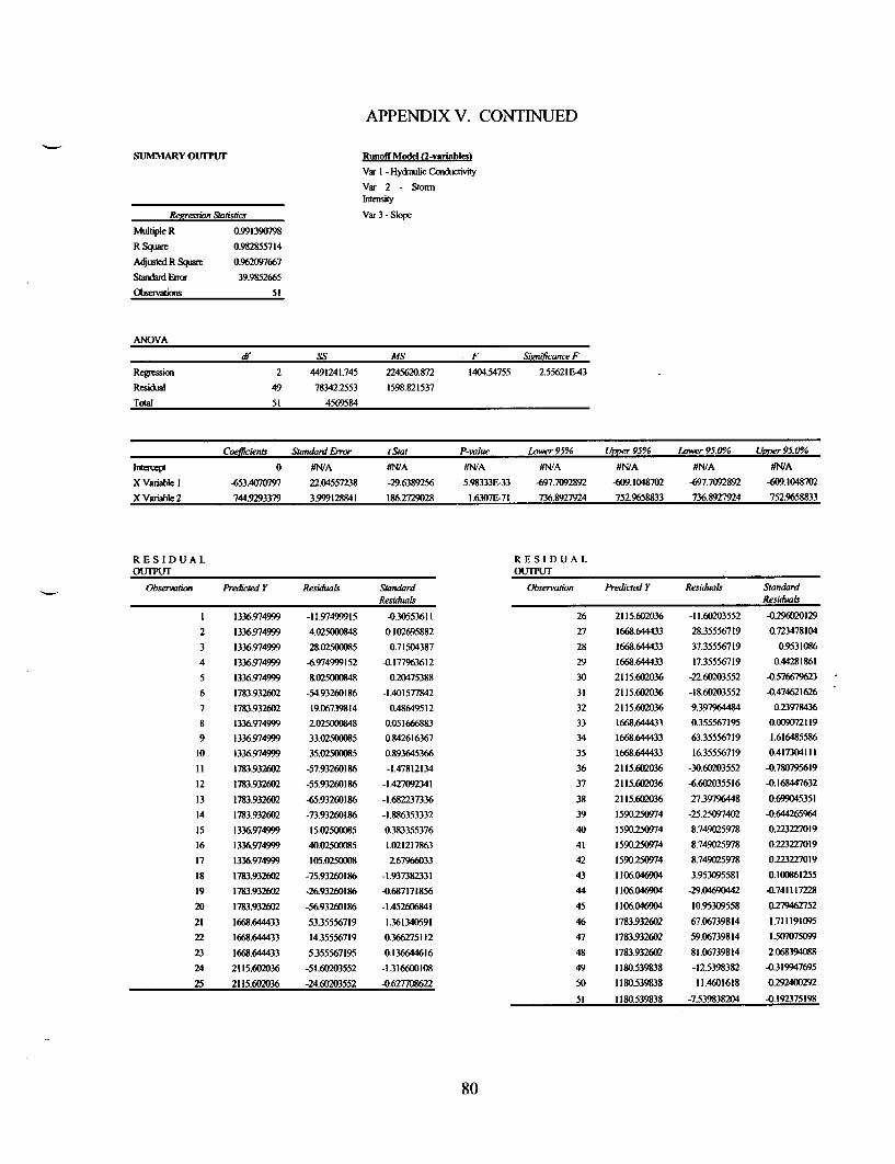
APPENDIX V. CONTINUED

SUMMARY Our'ur Runoff Model (2-variables)

Var I - Hydraulic Conidctivity

Var 2 - StormIntensity

Var 3 - SlopeRegression SralftdcS

Multiple R 0.991390798

R Square 0.982855714

Atjusled R Square 0.962097667

Standard Errrr 39.9852665

Observations 5 1

ANOVA

df SS MS F Significance F

Regression 2 4491241.745 2245620.872 1404.54755 2.55621E-43

Residual 49 78342.2553 1598.821537

Total 51 4569584

Coefficients Standard Error tStat P-wvue Lower 95% Upper 95% Lower 95.0% Upper 95.0%X

Interpt 0 #N/A #NA #NtA #N/A MNIA #N/A #N/A

X Variable 1 4653.4070797 2204557238 -29.6389256 5.98333E-33 -97.7092892 4609.1048702 -697.7092892 -609.1048702

X Variable 2 744.9293379 3.999128841 1861729028 1.6307E-71 736.8927924 75Z9658833 736.8927924 7529658833

RESIDUALOUI-PUr

Observeation Predicted Y Residuals StiandardResiduals

1 1336.974999 -11.97499915 030553611

2 1336.974999 4.025000848 0.102695882

3 1336.974999 28.02500085 0.71504387

4 1336.974999 -6.974999152 -0.177963612

5 1336.974999 8.025000848 0.20475388

6 1783.932602 -54.93260186 -1.401577842

7 1783.932602 19.06739814 0.48649512

8 1336.974999 2025000848 0.051666883

9 1336,974999 33.02500085 0.842616367

10 1336.974999 35.02500085 0.893645366

I 1 1783.932602 -57.93260186 -1.47812134

12 1783.932602 -55.93260186 -1.427092341

13 1783.932602 -65.93260186 -1.682237336

14 1783.932602 -73.93260186 -1.886353332

15 1336.974999 15.02500085 0383355376

16 1336.974999 40.02500085 1.021217863

17 1336.974999 105.0250008 2.67966033

18 1783.932602 -75.93260186 -1.937382331

19 1783.932602 -26.93260186 -0.687171856

20 1783.932602 -56,93260186 -1.452606841

21 1668.644433 53.35556719 1361340591

22 1668.644433 14.35556719 0.366275112

23 1668.644433 5355567195 0.136644616

24 2115.602036 -51.60203552 -1.316600108

25 2115.602036 -24.60203552 4.627708622

RESIDUALOUTPUT

Observation Predicted Y Residuals StandardResiduals

26 2115.602036 -11.60203552 -0.296020129

27 1668,644433 28.35556719 0.723478104

28 1668.644433 3735556719 0.9531086

29 1668.644433 1735556719 0.44281861

30 2115.602036 -2260203552 -0.576679623

31 2115.602036 -1860203552 -0.474621626

32 2115.602036 9397964484 023978436

33 1668.644433 0355567195 0.009072119

34 1668.644433 63.35556719 1.616485586

35 1668.644433 16.35556719 0.417304111

36 2115.602036 -30.60203552 -0.780795619

37 2115.602036 -6.602035516 -0.168447632

38 2115.602036 2739796448 0.699045351

39 1590.250974 -25.25097402 -0.644265964

40 1590250974 8.749025978 0.223227019

41 1590 974 8.749025978 0223227019

42 1590250974 8.749025978 022 727019

43 1106.046904 3.953095581 0.100861255

44 1106.046904 -29.04690442 -0.741117228

45 1106.046904 10.95309558 0279462752

46 1783.932602 67.06739814 1.711191095

47 1783.932602 59.06739814 1507075099

48 1783.932602 81.06739814 2068394088

49 1180-539838 -125398382 -0319947695

50 1180539838 11.4601618 0.292400292

51 1180.539838 -7.539838204 -0.197375198

80

APPENDIX V. CONTINUED

SUMNMARY OUTPUT

Regression Statistics

Multiple R 0.854467992

Ilration Model 0-variablesl

Va I - Hydrulic Cabxtivily

Var 2 - StonmIntensity

Var 3 - Slpe

R Square

Adusted R Square

S9mbad Ero

0.730115549

0.693454385

57.79309881

Obtvations 45

ANOVA

df SS MS F Siznificance F

Regeson 3 379502.8024 126500.9341 37.87405186 6.83667E-12

Residal 42 140281.7753 3340.04227

Total 45 519784.5778

Coefficients Standard Error t Stat P-value lower 95% Upper 95% Lower 95. 0% Upper 95.0%1

Tntcnt 0 #NIA fNIA #N/A #NdA 11N/A #NIA #NtA

X Variable 1 318.3324974 33.33447514 9.549647806 436E-12 251.0607817 385.604213 251.0607817 385.604213

X Variable 2 -17.11848864 8340568301 -2.052436719 0.046393082 -33.95044224 -0286535032 -33.95044224 -026535032

X Variable 3 13.28845083 2.853340669 4.657155372 3-21424E-05 7.530174408 19.04672724 7.530174408 19.04672724

RESIDUALOUTPUT

Observation Predicted r Residuals StandardResiduals

1 210.4292487 -57.42924874 -1.028581634

2 210.4292487 46.42924874 -0.831567077

3 210.4292487 . -42.42924874 -0.75992542

4 210.4292487 -32.42924874 -0.580821278

5 2104292487 -70.42924874 -1 261417019

6 200.1581556 -24.15815556 .0.432682573

7 200.1581556 47.15815556 .0.8446221

8 170.5638963 -33.56389627 -0.601143285

9 170.5638963 -11.56389627 -0.207114172

10 170.5638963 -14.56389627 -0.260845415

11 1602928031 43.70719691 0.782814001

12 1602928031 4529280309 0.811212865

13 1602928031 42.70719691 0.764903587

14 200.1581556 48.84184444 0.874777665

15 276.8715029 73.12849713 1.309761675

16 276.8715029 77.12849713 1381403332

17 276.8715029 61.12849713 1.094836705

18 266.6004097 146.3995903 2.622077305

19 266.609407 103.3995903 1.851929493

20 266.6004097 140.3995903 2.51461482

21 8.978320606 30.02167939 0.537700714

22 8.978320606 32-02167939 0.573521542

23 8.978320606 35.02167939 0.627252785

24 -1292772576 53.29277258 0.954495632

25 -12.92772576 5129277258 0.918674804

RESIDUALOuTPrU

Observation Predicted Y Residuals StandardResiduals

26 -1292772576 4729277258 0.847033147

27 48.84367308 -20.84367308 -0.194214677

28 48.84367308 -15.84367308 -0283766748

29 48.84367308 -15.84367308 -0283766748

30 38.5725799 7.427420101 0.133028171

31 38.5725799 9.427420101 0.168848999

32 385725799 6.427420101 0.115117756

33 1152859272 -74.28592721 -1330491727

34 1152859272 -7628592721 -1.366312556

35 1152859272 -7028592722 -1.25885007

36 105.014834 -44.01483403 -0.788323909

37 105.014834 47.01483403 -0.842055152

38 105.014834 42.01483403 -0.752503081

39 204.6089626 -22.60896261 -0.404935885

40 204.6089626 -64.60896261 -1.157173283

41 204.6089626 47.60896261 -0.852696241

42 204.6089626 -35.60896261 0.63777227

43 215.7359802 -48.73598022 -0.872881593

44 215.7359802 49.7359822 -0.890792008

45 215.7359802 -27.73598022 -0.496762895

81

APPENDIX V. CONTINUED

SUMIARY OIJTPUT Infiltration Model (3variales)

Var I - Hydaulic Comductivity

Var 2 - Stonn Itensity

Var 3 - SlopeRenvession Slatistics

Multiple R 0.87166837

R Square

Adjinted R SquareStadr Enro

0.75980574

0.7245584

50.8472803

Obsaervatiomi 45

ANOVA

df Ss MS F Signifitance F

Regession 3 343498.383 114499.461 44.286156 62934E-13

Residbnl 42 108588.728 2585.44591

Total 45 452087.111

Caefficients Standard Error IStal P-value Lawer 95% Upper 95% Lower 95.0%X Upper 95.0%,

titpt 0 MN/A #NtA #N/A #tNA #N/A NN/A MNA

X Variable 1 308.497034 293281972 10.5187861 2.4257E-13 249310317 367.683751 249310317 367.683751

XVariable2 21.9719938 73381636 2.99420876 0.00459743 7.16297538 36.7810121 7.16297538 367810121

XVariable3 -14.141946 2.51041414 -5.6333118 1.3358E-06 -19208168 -9.0757232 -19.208168 -9.0757232

RESIDUAL OUT fUI RESIDUAL OUTPUT

Observadon Prrdicted Y Residuals StandardResiduals Observation Predicted Y Residuals StandardResiduals

1 157-520149 9.47985088

2 157520149 40.4798509

3 157520149 36.4798509

4 157520149 3.47985088

5 157520149 547985088

6 170.703345 52.2966546

7 170.703345 55.2966546

8 199.945986 14.054014

9 199.945986 7.05401397

10 199.945986 3.05401397

11 213.129182 25.8708177

12 213.129182 42.8708177

13 213.129182 11.8708177

14 170.703345 -0.7033454

15 86.8104209 -86.810421

16 86.8104209 -83.810421

17 86.8104209 -85.810421

18 99.9936172 -78993617

19 99.9936172 -95.993617

20 99.9936172 -96.993617

21 433528915 43.352892

22 43.3528915 43352892

23 43.3528915 43352892

24 56.5360878 -56.536088

25 56.5360878 -55.536088

0.19298137

0.82404853

0.74262051

0.07083934

0. 11155335

1.06460326

1.12567427

0.28609763

0.14359860.06217058

0.52665237

0.87272145

0.2416543

-0.014318

-1.7672002

-1.7061292

-1.7468432

-1.6080735

-1.9541425

-1.9744996

-0.882535

-0.882535

-0.882535

-1.1509054

-1.1305484

26 56.5360878 -56.536088 -1.1509054

27 0.92705461 -0.9270546 -0.0188721

28 0.92705461 -0.9270546 -0.0188721

29 0.92705461 -0.9270546 -0.018872l

30 14.1102509 -14.110251 -0.2872424

31 14.1102509 -14.110251 -0.2872424

32 14.1102509 -1Z110251 -0.2465284

33 -69.782674 69.7826736 1.42056624

34 -69.782674 69.7826736 1.42056624

35 -69.782674 69.7826736 1.42056624

36 -56.599477 56.5994773 1.15219584

37 -56.599477 565994773 1.15219584

38 -56.599477 56.5994773 1.15219584

39 164.990627 14.009373 028518888

40 164.990627 -2.990627 -0.0608802

41 164.990627 47.009373 0.95697004

42 164.990627 43.009373 0.87554202

43 150.708831 532911689 1.08484859

44 150.708831 542911689 1.1052056

45 150.708831 829116894 0.16878337

82

APPENDIX V. CONTINUED

SUMMARY OUTrPUT

Regression Statistics

Multip R 0.955022

R Square 0.912066

Adusted R Square 0.842898

Leakafe Model (3-variablesone

Var I -Hydrk Cmlxmi

Var 2 - Storm Intensity

Var 3 - Slope

Stardard Ezr 30-20595

O01eivanon 20

ANOVA

df SS MS F Significance F

Regression 3 160881 53627 58.77578 7.37E-09

Rewal 17 15510.79 912.3997

Total 20 176391.8

Coeflcients StandardError t Stat P-whae Lower 95% Upper 95% Lower95.0%1* Upper 95.0%1.

Intercet 0 #UA #UN/A #NA UN/A #UNA #NIA #N/A

XVariabkle 3932411 1033987 3.803154 0.001421 175.0887 6113936 175.0887 6113936

XVariable2 29.96714 22.63179 1324117 0202993 -17.78184 77.71612 -17.78184 77.71612

X Variable 3 -28.504 2.153576 -13.23566 222E-10 -33.04766 -23.96035 -33.04766 -23.96035

RESIDUAL OUTPIUT

Observation Predicted Y Residuals Standard Residuals

2

3

4

5

6

7

8

9

10

II

12

13

14

15

16

17

18

19

20

152.9113

152.9113

152.9113

1529113

152.9113

170.8916

170.8916

238.4233

238.4233

238.4233

256.4036

2564036

256.4036

170.8916

10.39125

10.39125

1039125

2&37153

2837153

2837153

14.08872

45.08872

41.08872

8088725

10.08872

52.10844

55.10844

-24.42329

-31.42329

-35.42329

-17.40357

-0.403574

-31.40357

-0.891559

-1039125

-7.391251

-9391251

-7.371534

-2437153

-25.37153

0.505906

1.619071

1.475437

0.290454

0.362272

1.871139

1.978865

-0.877005

-1.128365

-1271999

0.624937

-0.014492

-1.127657

-0.032015

-0.373135

-0265409

.0.337226

-0264701

-0.875147

-0.911055

83

APPENDIX V. CONTINUED

SUMMARY o~umrr

Reg.ression Statistcs

MultileR 0.9773776

R Squam 0.95526698

A4wuateR.Squmi 092932731

Standmd Enm 57.8170744

OAbserWaons 45

Rttnoff4In~fitratn MMde

Var I -Hy~kmi Cohxtivily

Var 2 - Storm Intensity

Var 3 -SMope

AN4OVA

h Ss MS F 9wnificance F

Regesion 3 299818261 999394203 298.967928 6.914E-28

Residual 42 140398.192 3342.81409

Total 45 3138580.8

Cbowdenft Standaird Enor tSkat P-whe Lower95% Upper 95% Lowr 95.0%1 Upper 95.0%

iitpt 0 MNA MVA *NVA #WA MN/A UN/A UNA

X Vaiabl -346.63855 33348304 -10394488 3.49OIE-13 413.93818 -27933893 -41393818 -27933893

X Vaiable 2 719.60798 83440284 862725728 6.5941E-49 703.021861 736699734 703.021861 736.699734

X Vaiable 3 16,8531004 2.85452438 5.90399594 5.4587Ei07 11.0924351 22,6137656 11.0924351 22.6137656

RESIDUAL OUIPUT RESIDUAL OUTPUT

Observation Preficd Y Residuals Sandrd Residuals Observtion Predcted Y Residual StandardResiduah

1 154028153 -62.28153

2 1540.28153 -35.28153

3 1540.28153 -7.2815304

4 1540.28153 -3228153

5 1540.28153 -5528153

6 197219801 467.1980D9

7 1972.19801 -16,198009

8 1489.72223 -13.722229

9 1489.723 392777706

10 1489.72223 382777706

11 1921371 8.36129192

12 1921.63871 -78.638708

13 1921.63871 4.638708I

14 1972.19801 -13.198009

15 1624.54703 77.4529678

16 1624.54703 106.452968

17 1624.54703 155.452968

18 2056.46351 64.5364891

19 2056.46351 70.5364891

20 2056.46351 77.5364891

21 1665.67596 953240413

22 1665.67596 583240413

23 1665.67596 52.3240413

24 2097.59244 18.4075626

25 2097.59244 43.4075626

-1.1150254

4.6316448

4.1303611

4S779358

4.9897045

-12030451

-02899927

42456689

0.70318942

0.6S528643

01496921

-1.4078678

4.0114348

4236283S

138663949

1905V2611

Z7839724S

1.15539593

126281386

138813477

I.70658509

1.04417456

093675664

032955036

0.77712503

26 209759244 524075626

27 171623526 18.7647402

28 171623526 227647402

29 171623526 Z76474024

30 214S.15174 -9.1517385

31 2148.15174 -3.1517385

32 2148.15174 21.482615

33 180050076 -90.762

34 180DSC076 -29500762

35 1800.S076 -70.500762

36 2232.41724 4&41724

37 2232.41724 -65.41724

38 2232.41724 -241724

39 1785.0342 -38.034202

40 17S5.0342 -0426 2

41 1785.0342 -29.034202

42 1785.0342 -17.034202

43 1317.12468 40.124683

44 1317.12468 -74.124683

45 1317.12468 -12 124683

093825192

03359449

a40755685

004949711

4.163S435

4.0564255

0391 14915

-1.620234

4.5281518

-12621742

-15471267

-1.171164

4.4729475

4.6809258

4.8241497

45197989

-03049631

4.7183517

-1.3270532

4217068

84

APPENDIX VI. HELP MODEL RUNS

MPEMODELRUNS

** HYDROLOGIC EVALUATION OF LANDFILL PERFORMANCE** HELP MODEL VERSION 3.06 (17 AUGUST 1996) ***4 DEVELOPED BY ENVIRONMENTAL LABORATORY ***4 USAE WATERWAYS EXPERIMENT STATION *4as FORUSEPARISKREDUCIONENGNEERINGLABORATORY

TITLE RUNS(3-Iayu/IS99n Stoun/2% SkpI/.6E-4 ainsec Paem)

4*

*4

NOTE INITIAL MOISTURE CONTENT OF THE LAYERS AND SNOW WATERWERE SPECIFIED BY THE USER.

LAYER I

TYPE I - VERTICAL PERCOLATION LAYERMATERIAL TEXTURE NUMBER 10

THICKNESS = 6.00 INCHESPOROSITY = 03980 VOL/VOLFIELD CAPACITY = 02440 VOL/VOLWILTING POINT = 0.1360 VOLIVOLINITIAL SOIL WATER CONTENT = 02900 VOLIVOLEFFECTIVE SAT. HYD. COND. - 0.1 19999997000E-03 CM/SEC

LAYER 2

TYPE 2 - LATERAL DRAINAGE LAYERMATERIAL TEXTURE NUMBER 10

THICKNESS = 6.00 INCHESPOROSITY = 03980 VOL/VOLFIELD CAPACITY = 0.2440 VOL/VOLWILTING POINT - 0.1360VOL/VOLINITIAL SOIL WATER CONTENT = 0.2900 VOLIVOLEFFECTIVE SAT. HYD. COND. = 0.119999997000E-03 CM/SECSLOPE = 2.00 PERCENTDRAINAGE LENGTH = 8.0 FEET

LAYER 3

TYPE 4 - FLEXIBLE MEMBRANE LINERMATERIAL TEXTURE NUMBER 35

THICKNESS = 0.06 INCHESPOROSITY = 0.0000 VOL/VOLFIELD CAPACITY = 0.0000 VOLIVOLWILTING POINT = 0.0000 VOLIVOLINITIAL SOIL WATER CONTENT = 0.0000 VOLIVOLEFFECTIVE SAT. HYD. COND. = 0.199999996000E-12 CMISECFML PINHOLE DENSITY = 0.00 HOLES/ACREFML INSTALLATION DEFECTS = 1.00 HOLES/ACREFML PLACEMENT QUALITY = I - PERFECT

GENERAL DESIGN AND EVAPORATIVE ZONE DATA

NOTE: SCS RUNOFF CURVE NUMBER WAS COMPUTED FROM DEFAULTSOIL DATA BASE USING SOIL TEXTURE #10 WITH BAREGROUND CONDMONS, A SURFACE SLOPE OF 2.% ANDA SLOPE LENGTH OF & FEET.

SCS RUNOFF CURVE NUMBER = 94.90FRACTION OF AREA ALLOWING RUNOFF = 100.0 PERCENTAREA PROJECTED ON HORIZONTAL PLANE = 0.000 ACRESEVAPORATIVE ZONE DEPTH = 6.0 INCHESINITIAL WATER IN EVAPORATIVE ZONE = 1.740 INCHESUPPER LIMIT OF EVAPORATIVE STORAGE = 2388 INCHESLOWER LIMIT OF EVAPORATIVE STORAGE = 0.816 INCHESINITIAL SNOW WATER = 0.000 INCHESINITIAL WATER IN LAYER MATERIALS = 3.480 INCHESTOTAL INITIAL WATER = 3.480 INCHESTOTAL SUBSURFACE INFLOW = 0.00 INCHESIYEAR

85

EVAPOTRANSPIRATION AND WEATHER DATA

NOTE: EVAPOTRANSPIRATION DATA WAS OBTAINED FROMTAMPA FLORIDA

STATION LATITUDE = 27.58 DEGREESMAXIMUM LEAF AREA INDEX = 0.00START OF GROWING SEASON (JULIAN DATE) = 0END OF GROWING SEASON (JULIAN DATE) = 367EVAPORATIVE ZONE DEPTH = 6.0 INCHESAVERAGE ANNUAL WIND SPEED = 8.60 MPHAVERAGE IST QUARTER RELATIVE HUMIDITY 74.00%AVERAGE 2ND QUARTER RELATIVE HUMIDITY 72.00%AVERAGE 3RD QUARTER RELATIVE HUMIDITY 78.00 %AVERAGE 4TH QUARTER RELATIVE HUMIDITY 76.00 %

NOTE: PRECIPrTATION DATA FOR Tampa FkridaWAS ENTERED BY THE USER.

NOTE: TEMPERATURE DATA WAS SYNTHETICALLY GENERATED USINGCOEFFICIENTS FOR TAMPA FLORIDA

NORMAL MEAN MONTHLY TEMPERATURE (DEGREES FAHRENHEIT)JAN/JUL FE/AUG MAR/SEP APRIOCT MAYINOV JUALDEC

59.80 60.80 66.20 71.60 77.10 80.9082.20 82.20 80.90 74.50 66.70 61.30

NOTE: SOLAR RADIATION DATA WAS SYNTHETICALLY GENERATED USINGCOEFFICIENTS FOR TAMPA FLORIDAAND STATION LATITUDE = 27.58 DEGREES

HEAD #1: AVERAGE HEAD ON TOP OF LAYER 3DRAIN #1: LATERAL DRAINAGE FROM LAYER 2 (RECIRCULATION AND COLLECTION)

LEAK #1: PERCOLATION OR LEAKAGE THROUGH LAYER 3

DAILY OUIPUT FOR YEAR 1997

DAY A 0 RAIN RUNOFF Er E. ZONE HEAD DRAIN LEAK11 WATER #1 #1 #1R L IN. IN. TN. INJN. IN. IN. IN.

1 1.99 1.342 0.005 0.2869 3.4110.1298E-01 3489E-052 0.00 0.000 0.005 0.2803 6.2681 .3431E-01 .6412E-053 0.00 0.000 0.005 0.2737 6.2337 .3399E-01 .6377E-054 0.00 0.000 0.005 0.2669 6.3762 .3538E-01 .6523E-055 0.00 0.000 0.005 0.2602 6.3203 3482E-01 .6466E-056 0.00 0.000 0.005 0.2544 6.1775 3344E-01 .6320E-057 0.00 0.000 0.005 0.2504 5.9461 .3123E-01 .6083E-058 0.00 0.000 0.005 02468 5.8596.3043E-01 .5994E-059 0.00 0.000 0.005 0.2434 5.7670.2958E-01 .5900E-0510 0.00 0.000 0.005 0.2404 5.6696.2870E-01 .5800E-05

AVERAGE ANNUAL TOTALS & (STD. DEVIATIONS) FOR YEARS 1997 THROUGH 1997

INCHES CU. FEET PERCENT

PRECIPITATION 1.99 ( 0.000) 2.9 100.00RUNOFF 1.342 ( 0.0000) 1.95 67A57EVAPOTRANSPIRATION 0.672 ( 0.0000) 0.98 33.758LATERAL DRAINAGE COLLECTED 1.16706( 0.00000) 1.695 58.64628

FROM LAYER 2PERCOLATIONILEAKAGE THROUGH 0.00037 ( 0.00000) 0.001 0.01869

LAYER 3AVERAGE HEAD ON TOP 1.002 ( 0.000)

OF LAYER 3CHANGE IN WATER STORAGE -1.192 ( 0.0000) -1.73 -59.880

86

APPENDIX VI. CONTINUE

HYDROLOGIC EVALUATION OF LANDFILL PERFORMANCE **

HELP MODEL VERSION 3.06 (17 AUGUST 1996) **** DEVELOPED BY ENVIRONMENTAL LABORATORY **

by USAE WATERWAYS EXPERIMENT STATION** FOR USEPA RISK REDUCTION ENGINEERING LABORATORY *e

TTLhE RUNS(3-layeulI99f StWrJO2% SlodI.9E-5an/sec Perm)

NOTE INITIAL MOISTURE CONTENT OF THE LAYERS AND SNOW WATERWERE SPECIFIED BY THE USER.

LAYER I

TYPE I - VERTICAL PERCOLATION LAYERMATERIALTEXTURENUMBER 15

THICKNESS 6.00 INCHESPOROSITY = 0.4750 VOLNOLFIELD CAPACITY = 03780 VOIJVOLWILTING POINT = 02650 VOLIVOLINITIAL SOIL WATER CONTENT - 02650 VOL/VOLEFFECIVE SAT.HYD.COND. = 0.170000003000E-04CM/SEC

LAYER 2

TYPE 2 - LATERAL DRAINAGE LAYERMATERIAL TEXTURE NUMBER 15

THICKNESS = 6.00 INCHESPOROSITY = 0.4750 VOLNOLFIELD CAPACITY = 03780 VOLIVOLWILTING POINT = 02650 VOL/VOLINITIAL SOIL WATER CONTENT = 0.2650 VOL/VOLEFFECTIVE SAT. HYD. COND. = 0.1700D0003000E-04 CM/SECSLOPE - 2.00 PERCENTDRAINAGE LENGTH = 8.0 FEET

LAYER 3

TYPE 4 - FLEXIBLE MEMBRANE LINERMATERIAL TEXTURE NUMBER

THICKNESS = 0.06 INCHESPOROSITY = 0.0000 VOL/VOLFIELD CAPACITY = 0.0000 VOLIVOLWILTING POINT 0.0000 VOL/VOLINITIAL SOIL WATER CONTENT = 0.0000 VOL/VOLEFFECTVE SAT. HYD. COND. = 0.199999996000E-12 CM/SECFML PINHOLE DENSITY = 0.00 HOLES/ACREFML INSTALLATION DEFECTS = 1.00 HOLES/ACREFML PLACEMENT QUALITY = I - PERFECT

GENERAL DESIGN AND EVAPORATIVE ZONE DATA

NOTEl SCS RUNOFF CURVE NUMBER WAS COMPUTED FROM DEFAULTSOIL DATA BASE USING SOIL TEXTURE #15 WITH BAREGROUND CONDITIONS, A SURFACE SLOPE OF 1% ANDA SLOPE LENGTH OF 8. FEET.

SCS RUNOFF CURVE NUMBER = 97.10FRACTION OF AREA ALLOWING RUNOFF = 100.0 PERCENTAREA PROJECTED ON HORIZONTAL PLANE = 0.000 ACRESEVAPORATIVE ZONE DEPTH = 6.0 INCHESINITAL WATER IN EVAPORATIVE ZONE = 1.590 INCHESUPPER LIMIT OF EVAPORATIVE STORAGE = 2.850 INCHESLOWER LIMIT OF EVAPORATIVE STORAGE = 1.590 INCHESINlllAL SNOW WATER = 0.000 INCHESINITIAL WATER IN LAYER MATERIALS - 3.180 INCHESTOTAL INITIAL WATER = 3.180 INCHESTOTAL SUBSURFACE INFLOW = O.00 INCHES/YEAR

EVAPOTRANSPIRATION AND WEATHER DATA

87

NOTE EVAPOTRANSPIRATION DATA WAS OBTAINED FROMTAMPA FLORIDA

STATIONLATITUDE = 2758 DEGREESMAXIMUM LEAF AREA INDEX = 0.00START OF GROWING SEASON (JULIAN DATE) = 0END OF GROWING SEASON (RUMIAN DATE) = 367EVAPORATIVE ZONE DEPTH = 6.0 INCHESAVERAGE ANNUAL WIND SPEED = 8.60 MPHAVERAGE 1ST QUARTER RELATIVE HUMIDITY =74.00 %AVERAGE 2ND QUARTER RELATIVE HUMIDIlY 72.00 %AVERAGE 3RD QUARTER RELATIVE HUMIDITY = 78.00 %AVERAGE 4TH QUARTER RELATIVE HUMIDITY =76.00 %

NOTE PRECIPITATION DATA FOR Tampa FloridaWAS ENTERED BY THE USER.

NOTE: TEMPERATURE DATA WAS SYNTHETICALLY GENERATED USINGCOEFFICIENTS FOR TAMPA FLORIDA

NORMAL MEAN MONTHLY TEMPERATURE (DEGREES FAHRENHEI)JANUUL FEB/AUG MAR/SEP APR/OCT MAY/NOV JUNIDEC

59.80 60.80 66.20 71.60 77.10 80.9082.20 8220 80.90 74.50 66.70 61.30

NOTE: SOLAR RADIATION DATA WAS SYNTHETICALLY GENERATED USINGCOEFFICIENTS FOR TAMPA FLORIDA

AND STATION LATITUDE = 27.58 DEGREES

HEAD #1: AVERAGE HEAD ON TOP OF LAYER 3DRAIN #1: LATERAL DRAINAGE FROM LAYER 2 (RECIRCULATION AND COLLECION)LEAK #1: PERCOLATION OR LEAKAGE THROUGH LAYER 3

DAILY OUIPUT FOR YEAR 1997

DAY A 0 RAIN RUNOFF ET E ZONE HEAD DRAIN LEAKI I WATER #l #1 #1R L IN. IN. IN. INAN. IN. IN. IN.

1 1.99 1.392 0.005 0.3639 0.0000 .0000E+00 .0000E002 0.00 0.000 0.004 0.3632 0.0000 .0000E+00.OOOOE+003 0.00 0.000 0.005 0.3624 0.0000.0000E+00.00001E+004 0.00 0.000 0.005 0.3616 0.0000.OOOOE+00.OOOE+O05 0.00 0.000 0.005 0.3609 0.0000 . OOOOE+000001E{06* 0.00 0.000 0.005 0.3601 0.0000.00001E+00.00001E+007 0.00 0.000 0.005 0.3593 0.0000 .0000E+00.OOOOE+008 0.00 0.000 0.005 0.3586 0.0000.0000E+00.OOOOE-u1009 0.00 0.000 0.005 0.3578 0.0000 .003E+00.0000E+0010 0.00 0.000 0.005 0.3570 0.0000.0000E+00.0000E+00

AVERAGE ANNUAL TOTALS & (SD. DEVIATIONS) FOR YEARS 1997 THROUGH 1997

INCHES CU. FEET PERCENT

PRECIPITATION 1.99 ( 0.000) 2.9 100.00RUNOFF 1.392 ( 0.0000) 2.02 69.941EVAPOTRANSPIRATION 0.566 ( 0.0000) 0.82 28.422LATERAL DRAINAGE COLLECTED 0.00000( 0.00000) 0.000 0.00000

FROM LAYER 2PERCOLATIONLEAKAGE THROUGH 0.00 ( 0.00000) 0.000 O.OO0

LAYER 3AVERAGE HEAD ON TOP 0.000( 0.000)OF LAYER 3

CHANGE IN WATER STORAGE 0.033 ( 0.0000) 0.05 1.637

88

APPENDIX VI. CONTINUE

** HYDROLOGIC EVALUATION OF LANDFILL PERFORMANCEHL MODEL VERSION 3.06 (17 AUGUST 1996)

DEVELOPED BY ENVIRONMNAL LAORATORY **

USAE WATERWAYS EXPERIMENT STATIONFOR USEPA RISK REDUCTION ENGINEERING LABORATORY

TltE RUNS(199 in Stcwmi2t Slope/ 1.6E-5 an/sec Perm)

*0

NOTE: INmTlAL MOISTURE CONlENT OF THE LAYERS AND SNOW WATERWERE SPECIFIED BY THE USER.

LAYER I

TYPE I - VERTICAL PERCOLATION LAYERMATERIAL TEXTURE NUMBER 10

THICKNESS = 6.00 INCHESPOROSITY 5 03980 VOL/VOLFIELD CAPACITY - 02440 VOL/COLWILTING POINT = 0.1360VOLJVOLINIlIAL SOIL WATER CONTENT = 02900 VOUVOLEFFECTIVE SAT. HYD. COND. = 0.1 19999997000E.03 CM/SEC

LAYER 2

TYPE 2 - LATERAL DRAINAGE LAYERMATERIAL TEXTURE NUMBER 10

THICKNESS 6.00 INCHESPOROSITY 0.3980 VOLNVOLFIELD CAPACITY - 0.2440 VOLIVOLWILTING POINT = 0.1360VOLIVOLINITIAL SOIL WATER CONTENT = 02900 VOLVOLEFFECTIVE SAT. HYD. COND. = 0.1 19999997000E-03 CM/SEC

LAYER 3

TYPE 2 - LATERAL DRAINAGE LAYERMATERIAL TEXTURE NUMBER 0

THICKNESS = 0.10 INCHESPOROSITY - 03500 VOL/VOLFIELD CAPACITY = 0.0100 VOLIVOLWILTING POINT = 0.0050 VOIJVOLINTIIAL SOIL WATER CONTENT = 0.0050 VOLIVOLEFFECTIVE SAT. HYD. COND. = 0.400000019000E-02 CM/SEC

LAYER 4

TYPE 2 - LATERAL DRAINAGE LAYERMATERIAL TEXTURE NUMBER 34

THICKNESS = 0.12 INCHES

89

POROSITY = 0.8500 VOL/VOLFIELD CAPACITY = 0.0100 VOLIVOLWILTING POINT = 0.0050 VOLNOLINITIAL SOIL WATER CONTENT = 0.0050 VOLNOLEFFECTIVE SAT. HYD. COND. = 33.0000000000 CM/SECSLOPE = 2.00 PERCENTDRAINAGE LENGTH = 8.0 FEET

LAYER 5

TYPE 4 - FLEXIBLE MEMBRANE LINERMATERIAL TEXTURE NUMBER 35

THICKNESS = 0.06 INCHESPOROSITY = 0.0000 VOLNOLFIELD CAPACITY = 0.0000 VOLNOLWILTING POINT = 0.0000 VOL/VOLINITIAL SOIL WATER CONTENT = 0.0000 VOLNOLEFFECTIVE SAT. HYD. COND. = 0.199999996000E-12 CM/SECFML PINHOLE DENSITY = 0.00 HOLES/ACREFML INSTALLATION DEFECTS 1.00 HOLES/ACREFML PLACEMENT QUALITY = I - PERFECT

GENERAL DESIGN AND EVAPORATIVE ZONE DATA

NOTE. SCS RUNOFF CURVE NUMBER WAS COMPLIED FROM DEFAULTSOIL DATA BASE USING SOIL TEXTURE #10 WITH BAREGROUND CONDmONS, A SURFACE SLOPE OF 2.%. ANDA SLOPE LENGTH OF 8. FEET.

SCS RUNOFF CURVE NUMBER = 94.90FRACTION OF AREA ALLOWING RUNOFF = 100.0 PERCENTAREA PROJECTED ON HORIZONTAL PLANE = 0.000 ACRESEVAPORATIVE ZONE DEPTH = 6.0 INCHESINITIAL WATER IN EVAPORATIVE ZONE = 1.740 INCHESUPPER LIMIT OF EVAPORATIVE STORAGE = 2.388 INCHESLOWER LIIT OF EVAPORATIVE STORAGE = 0.816 INCHESINITIAL SNOW WATER = 0.000 INCHES

INITIAL WATER IN LAYER MATERIALS - 3A81 INCHESTOTAL INITIAL WATER = 3.481 INCHESTOTAL SUBSURFACE INFLOW = 0.00 INCHES/YEAR

EVAPOTRANSPIRATION AND WEATHER DATA

NOTE: EVAPOTRANSPIRATION DATA WAS OBTAINED FROMTAMPA FLORIDA

STATION LAITMUDE = 27.58 DEGREESMAXIMUM LEAF AREA INDEX = 0.00START OF GROWING SEASON (JULIAN DATE = 0END OF GROWING SEASON (JULIAN DATE) - 367EVAPORATIVE ZONE DEPTH = 6.0 INCIESAVERAGE ANNUAL WIND SPEED = 8.60 MPHAVERAGE I ST QUARTER RELATIVE HUMIDITY =74.00 %AVERAGE 2ND QUARTER RELATIVE HUMIDITY -72.00 %AVERAGE 3RD QUARTER RELATIVE HUMIDTY = 78.00 %AVERAGE 4TH QUARTER RELATIVE HUMIDITY = 76.00 %

NOTE: PRECIPITATION DATA FOR Tampa FloridaWAS ENTERED BY THE USER.

NOTE: TEMPERATURE DATA WAS SYNHETICALLY GENERATED USING

90

COEFF{CIENTS FOR TAMPA FLORIDA

NORMAL MEAN MONTHLY TEMPERATURE (DEGREES FAHRENHEI1)

JAN/JUL FEB/AUG MAR/SEP APRIOC[ MAY/NOV JUNDEC

59.80 60.80 66.20 71.60 77.10 80.9082.0 82.20 80.90 74.50 66.70 61.30

NOTE SOLAR RADIATION DATA WAS SYNTHETICALLY GENERATED USINGCOEFFICIENTS FOR TAMPA FLORIDA

AND STATION LAITTUDE 2758 DEGREES

HEAD #1: AVERAGE HEAD ON TOP OF LAYER 5DRAIN #1: LATERAL DRAINAGE FROM LAYER 4 (RECIRCULATION AND COLLECTION)LEAK #1: PERCOLATION OR LEAKAGE THROUGH LAYER 5

DAILY OUTPUT FOR YEAR 1997

SDAY A 0 RAIN RUNOFF ET E. ZONE HEAD DRAIN LEAK

I I WATER #1 #1 #1R L IN. IN. IN. INJIN. IN. IN. IN.

1 1.99 1.342 0.005 0.3476 0.0001..1604E-01 .7852E-042 0.00 0.000 0.005 0.2913 0.0016.4073 5402E-033 0.00 0.000 0.005 0.2766 0.0007.1763 .3631E-034 0.00 0.000 0.005 02679 0.0004.1000E+00.2746E-035 0.00 0.000 0.005 0.2619 0.0003.6912E-01 .2283E-036 0.00 0.000 0.005 0.2570 0.0002.5245E-01 .1991E-037 0.00 0.000 0.005 0.2529 0.0002.4139E-01 .1769E-038 0.00 0.0C0 0.005 0.2490 0.0001 .3379E-01 .1597E-039 0.00 0.000 0.005 0.2455 0.0001 .2932E-01 .1487E-0310 0.00 0.000 0.005 0.2422 0.0001 .2631E-01.1409E-03

AVERAGE ANNUAL TOTALS & (STD. DEVIATIONS) FOR YEARS 1997 THROUGH 1997

INCHES CU. FEET PERCENT

PRECIPITATION 1.99 ( 0.000) 2.9 100.00RUNOFF 1.342 ( 0.0000) 1.95 67.457EVAPOTRANSPIRATION 0.674 ( 0.0000) 0.98 33.881LATERAL DRAINAGE COLLECTED 1.16552 ( 0.00000) 1.692 5856909FROM LAYER 4

PERCOLATION/LEAKAGE THROUGH 0.00442 ( 0.00000) 0.006 0212LAYER S

AVERAGE HEAD ON TOP 0.000 ( 0.000)OF LAYER 5

CHANGE IN WATER STORAGE -1.197 ( 0.0000) -1.74 -60.129

91